The degree distribution - Computer Science Departmentcsn/slides/02degree_distribution.pdf · The degree distribution ... the proportion of vertices of degree k, which de nes ... web

OutlineVisual fitting

Non-linear regressionLikelihood

The challenge of parsimony

The degree distribution

Ramon Ferrer-i-Cancho & Argimiro Arratia

Universitat Politecnica de Catalunya

Version 0.4Complex and Social Networks (2016-2017)

Master in Innovation and Research in Informatics (MIRI)

Ramon Ferrer-i-Cancho & Argimiro Arratia The degree distribution




Official website: www.cs.upc.edu/~csn/

Contact:

I Ramon Ferrer-i-Cancho, [email protected],http://www.cs.upc.edu/~rferrericancho/

I Argimiro Arratia, [email protected],http://www.cs.upc.edu/~argimiro/


www.cs.upc.edu/~csn/

http://www.cs.upc.edu/~rferrericancho/

http://www.cs.upc.edu/~argimiro/




Visual fitting

Non-linear regression

Likelihood






The limits of visual analysis

A syntactic dependency network [Ferrer-i-Cancho et al., 2004]





The empirical degree distribution

I N: finite number of vertices / k vertex degree

I n(k): number of vertices of degree k.

I n(1),n(2),...,n(N) defines the degree spectrum (loops areallowed).

I n(k)/N: the proportion of vertices of degree k , which definesthe (empirical) degree distribution.

I p(k): function giving the probability that a vertex has degreek, p(k) ≈ n(k)/N.

I p(k): probability mass function (pmf).





Example: degree spectrum

I Global syntacticdependency network(English)

I Nodes: words

I Links: syntacticdependencies

Not as simple:

I Many degrees occurringjust once!

I Initial bending or hump:power-law?





Example: empirical degree distribution

I Notice the scale of they -axis.

I Normalized version of thedegree spectrum (dividingover N).





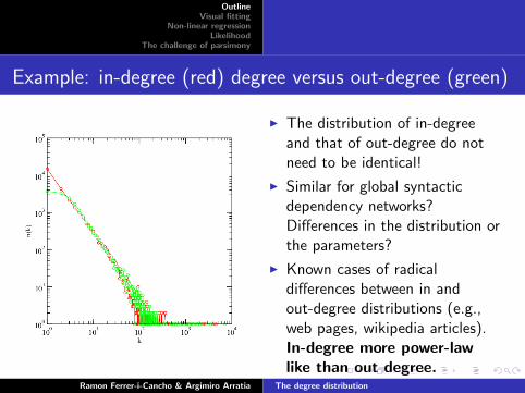
Example: in-degree (red) degree versus out-degree (green)

I The distribution of in-degreeand that of out-degree do notneed to be identical!

I Similar for global syntacticdependency networks?Differences in the distribution orthe parameters?

I Known cases of radicaldifferences between in andout-degree distributions (e.g.,web pages, wikipedia articles).In-degree more power-lawlike than out degree.





What is the mathematical form of p(k)?

Possible degree distributionsI The typical hypothesis: a power-law p(k) = ck−γ but what

exactly? How many free parameters?I Zeta distribution: 1 free parameter.I Right-truncated zeta distribution: 2 free parameters.I ...

Motivation:

I Accurate data description (looks are deceiving).

I Help to design or select dynamical models.





Zeta distributions I

Zeta distribution:

p(k) =1

ζ(γ)k−γ ,

being

ζ(γ) =∞∑x=1

x−γ

the Riemann zeta function.

I (here it is assumed that γ is real) ζ(γ) converges only forγ > 1 (γ > 1 is needed).

I γ is the only free parameter!

I Do we wish p(k) > 0 for k > N?





Zeta distributions I

Right-truncated zeta distribution

p(k) =1

H(kmax , γ)k−γ ,

being

H(kmax , γ) =kmax∑x=1

x−γ

the generalized harmonic number of order kmax of γ.Or why not

p(k) = ck−γe−kβ

(modified power-law, Altmann distribution,...) with 2 or 3 freeparameters?Which one is best? (standard model selection)





What is the mathematical form of p(k)?

Possible degree distributions

I The null hypothesis (for a Erdos-Renyi graph without loops)

p(k) =

(N − 1

k

)πk(1− π)N−1−k

with π as the only free parameter (assuming that N is givenby the real network).Binomial distribution with parameters N − 1 and π, thus〈k〉 = (N − 1)π ≈ Nπ.

I Another null hypothesis: random pairing of vertices withconstant number of edges E .





The problems II

I Is f (k), a good candidate? Does f (k) fit the empirical degreedistribution well enough?

I f (k) is a (candidate) model.I How do we evaluate goodness of a model? Three major

approaches:I Qualitatively (visually).I The error of the model: the deviation between the model and

the data.I The likelihood of the model: the probability that the model

produces the data.





Visual fitting

Assume a two variables: a predictor x (e.g., k , vertex degree) anda response y (e.g., n(k), the number vertices of degree k ; orp(k)...).

I Look for a transformation of the at least one of the variablesshowing approximately a straight line (upon visual inspection)and obtain the dependency between the two original variables.

I Typical transformations: x ′ = log(x), y ′ = log(y).

1. If y ′ = log(y) = ax + b (linear-log scale) theny = eax+b = ceax , with c = eb (exponential).

2. If y ′ = log(y) = ax ′ + b = alog(x) + b (log-log scale) theny = ealog(x)+b = cxa, with c = eb (power-law).

3. If y = ax ′ + b = alog(x) + b (log-linear scale) then thetransformation is exactly the functional dependency betweenthe original variables (logarithmic).





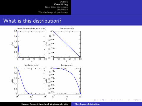
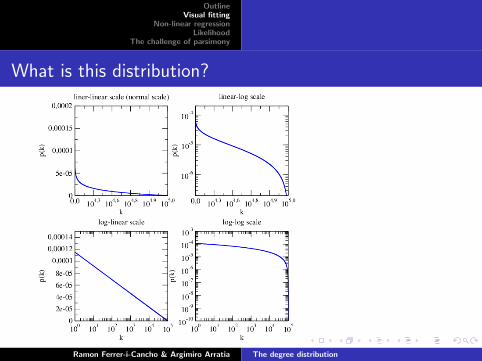
What is this distribution?





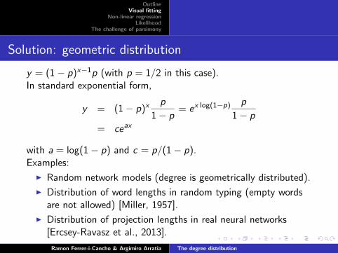
Solution: geometric distribution

y = (1− p)x−1p (with p = 1/2 in this case).In standard exponential form,

y = (1− p)xp

1− p= ex log(1−p) p

1− p

= ceax

with a = log(1− p) and c = p/(1− p).Examples:

I Random network models (degree is geometrically distributed).

I Distribution of word lengths in random typing (empty wordsare not allowed) [Miller, 1957].

I Distribution of projection lengths in real neural networks[Ercsey-Ravasz et al., 2013].





A power-law distribution

What is theexponent of thepower-law?





Solution: zeta distribution

y =1

ζ(a)x−a

with a = 2.Formula for ζ(a) is known for certain integer values, e.g.,ζ(2) = π2/6 ≈ 1.645.Examples:

I Empirical degree distribution of global syntactic dependencynetworks [Ferrer-i-Cancho et al., 2004] (but see also labsession on degree distributions).

I Frequency spectrum of words in texts [Corral et al., 2015].





What is this distribution?





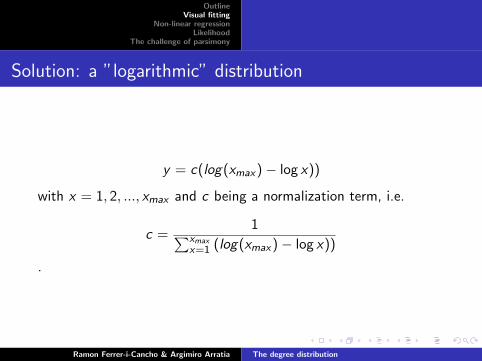
Solution: a ”logarithmic” distribution

y = c(log(xmax)− log x))

with x = 1, 2, ..., xmax and c being a normalization term, i.e.

c =1∑xmax

x=1 (log(xmax)− log x))

.





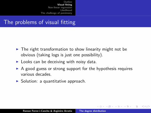
The problems of visual fitting

I The right transformation to show linearity might not beobvious (taking logs is just one possibility).

I Looks can be deceiving with noisy data.

I A good guess or strong support for the hypothesis requiresvarious decades.

I Solution: a quantitative approach.





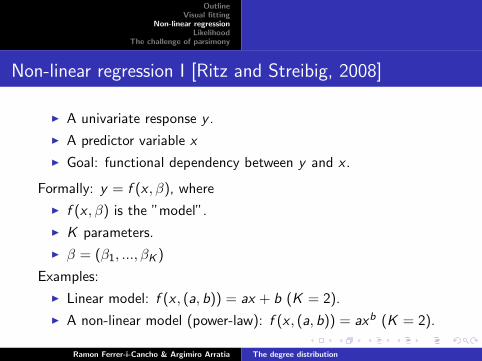
Non-linear regression I [Ritz and Streibig, 2008]

I A univariate response y .

I A predictor variable x

I Goal: functional dependency between y and x .

Formally: y = f (x , β), where

I f (x , β) is the ”model”.

I K parameters.

I β = (β1, ..., βK )

Examples:

I Linear model: f (x , (a, b)) = ax + b (K = 2).

I A non-linear model (power-law): f (x , (a, b)) = axb (K = 2).





Non-linear regression II

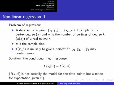
Problem of regression:

I A data set of n pairs: (x1, y1), ..., (xn, yn). Example: xi isvertex degree (k) and yi is the number of vertices of degree k(n(k)) of a real network.

I n is the sample size.

I f (x , β) is unlikely to give a perfect fit. y1, y2, ..., yn maycontain error.

Solution: the conditional mean response

E (yi |xi ) = f (xi , β)

(f (x , β) is not actually the model for the data points but a modelfor expectation given xi ).





Non-linear regression II

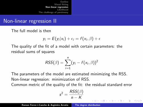
The full model is then

yi = E (yi |xi ) + εi = f (xi , β) + ε

The quality of the fit of a model with certain parameters: theresidual sums of squares

RSS(β) =n∑

i=1

(yi − f (xi , β))2

The parameters of the model are estimated minimizing the RSS.Non-linear regression: minimization of RSS.Common metric of the quality of the fit: the residual standard error

s2 =RSS(β)

n − K





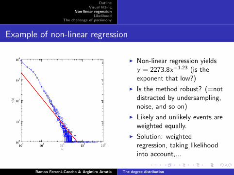
Example of non-linear regression

I Non-linear regression yieldsy = 2273.8x−1.23 (is theexponent that low?)

I Is the method robust? (=notdistracted by undersampling,noise, and so on)

I Likely and unlikely events areweighted equally.

I Solution: weightedregression, taking likelihoodinto account,...





Likelihood I [Burnham and Anderson, 2002]

I A probabilistic metric of the quality of the fit.

I L(parameters|data,model): likelihood of the parameters giventhe data (sample of size n) and a model.Example: L(γ|data,Zeta distribution with parameterγ)

I Best parameters: the parameters that maximizeL(parameters|data,model).





Likelihood II

I Consider a sample x1, x2, ...xn (e.g., the degree sequence of anetwork).

I Definition (assuming independence)

L(parameters|data,model) =∏i=1

p(xi ; parameters)

I For a zeta distribution

L(γ|x1, x2, .., xn; Zeta distribution) =n∏

i=1

p(xi ; γ)

= ζ(γ)−nn∏

i=1

x−γi





Log-likelihood

Likelihood is a vanishingly small number. Solution: taking logs.

L(parameters|data,model) = log L(parameters|data,model)

=∑i=1

log p(xi ; parameters)

Example:

L(γ|x1, x2, .., xn; Zeta distribution) =n∑

i=1

log p(xi ; γ)

= γ

n∑i=1

log xi − n log(ζ(γ))





Question to the audience

What is the best model for data?

Cue: a universal method.





What is the best model for data?

I The best model of the data is the data itself. Overfitting!

I The quality of the fit cannot decrease if more parameters areadded (wisely). Indeed, the quality of the fit normallyincreases when adding parameters.

I The metaphor of picture compression. Compressing a picture(with quality reduction). A good compression technique showsa nice trade-off between file size and image quality).

I Modelling is compressing a sample, the empirical distribution(e.g., compressing the degree sequence of a network).

I Models with many parameters should be penalized!I Models compressing the data with a low quality should be also

penalized.

How?





Akaike’s information criterion (AIC )

AIC = −2L+ 2K ,

with K being the number of parameters of the model. For smallsamples, a correction is necessary

AICc = −2L+ 2K

(n

n − K − 1

),

or equivalently

AICc = −2L+ 2K +2K (K + 1)

n − K − 1

= AIC +

(2K (K + 1)

n − K − 1

)AICc is recommended if n� K is not satisfied!





Model selection with AIC

I What is the best of a set of models? The model thatminimizes AIC

I AICbest : the AIC of the model with smallest AIC .

I ∆: ”AIC difference”, the difference between the AIC of themodel and that of the best model (∆ = 0 for the best model).





Example of model selection with AIC

Consider the case of model selection with three nested models:

Model 1 p(k) = k−2

ζ(2) (zeta distribution with (-)2 exponent)

Model 2 p(k) = k−γ

ζ(γ) (zeta distribution)

Model 3 p(k) = k−γ

H(kmax ,γ) (right-truncated zeta distribution)

Model i is nested model of i − 1 if the model i is a generalizationof model i − 1 (adding at least one parameter).





Example of model selection with AIC

Model K L AIC ∆

1 0 ... ... ....2 1 ... ... ....3 2 ... ... ....

Imagine that the true model is a zeta distribution with γ = 1.5 andthe sample is large enough, then

Model K L AIC ∆

1 0 ... ... � 02 1 ... ... 03 2 ... ... > 0





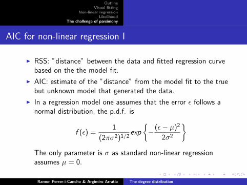
AIC for non-linear regression I

I RSS: ”distance” between the data and fitted regression curvebased on the the model fit.

I AIC: estimate of the ”distance” from the model fit to the truebut unknown model that generated the data.

I In a regression model one assumes that the error ε follows anormal distribution, the p.d.f. is

f (ε) =1

(2πσ2)1/2exp

{−(ε− µ)2

2σ2

}The only parameter is σ as standard non-linear regressionassumes µ = 0.





AIC for non-linear regression II

I Applying µ = 0 and εi = yi − f (xi , β)

f (εi ) =1

(2πσ2)1/2exp

{−(yi − f (xi , β))2

2σ2

}I Likelihood in a regression model:

L(β, σ2) =n∏

i=1

f (εi )

I After some algebra one gets

L(β, σ2) =1

(2πσ2)n/2exp

{−RSS(β)

2σ2

}.





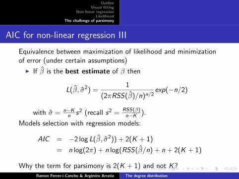
AIC for non-linear regression III

Equivalence between maximization of likelihood and minimizationof error (under certain assumptions)

I If β is the best estimate of β then

L(β, σ2) =1

(2πRSS(β)/n)n/2exp(−n/2)

with σ = n−Kn s2 (recall s2 = RSS(β)

n−K ).

Models selection with regression models:

AIC = −2 log L(β, σ2)) + 2(K + 1)

= n log(2π) + n log(RSS(β/n) + n + 2(K + 1)

Why the term for parsimony is 2(K + 1) and not K?Ramon Ferrer-i-Cancho & Argimiro Arratia The degree distribution




Concluding remarks

I Under non-linear regression AIC is the way to go for modelselection if the models are not nested (alternative methods doexist for nested models [Ritz and Streibig, 2008]).

I Equivalence between maximum likelihood and non-linearregression implies some assumption (e.g., homocedasticity).





Burnham, K. P. and Anderson, D. R. (2002).Model selection and multimodel inference. A practicalinformation-theoretic approach.Springer, New York, 2nd edition.

Corral, A., Boleda, G., and Ferrer-i-Cancho, R. (2015).Zipf’s law for word frequencies: word forms versus lemmas inlong texts.PLoS ONE, 10:e0129031.

Ercsey-Ravasz, M., Markov, N., Lamy, C., VanEssen, D.,Knoblauch, K., Toroczkai, Z., and Kennedy, H. (2013).A predictive network model of cerebral cortical connectivitybased on a distance rule.Neuron, 80(1):184 – 197.

Ferrer-i-Cancho, R., Sole, R. V., and Kohler, R. (2004).





Patterns in syntactic dependency networks.Physical Review E, 69:051915.

Miller, G. A. (1957).Some effects of intermittent silence.Am. J. Psychol., 70:311–314.

Ritz, C. and Streibig, J. C. (2008).Nonlinear regression with R.Springer, New York.


Documents

The degree distribution - Computer Science Departmentcsn/slides/02degree_distribution.pdf · The degree distribution ... the proportion of vertices of degree k, which de nes ... web