SOUTHERN JOURNAL OF AGRICULTURAL ECONOMICS DECEMBER, 1988

THE DEMAND AND SUPPLY OF U.S. AGRICULTURALEXPORTS: THE CASE OF WHEAT, CORN, AND SOYBEANSTassos Haniotis, John Baffes, and Glenn C. W. Ames

Abstract terms (in 1986, wheat, corn, and soybeansstill represented 70 percent of total U.S. ex-

The demand for and supply of U.S. wheat, ports compared to 75 percent in 1981), theircorn, and soybean exports is specified in a share of the total value of U.S. farm exportsdynamic framework. Obtained results indicate declined from 50 percent to 38 percent.differences in the export behavior of each pro- i i i i U. . iduct. U.S. corn exports are elastic, while U.S. tde performanc ha n agriculturalsoybean exports exhibit an inelastic response. tra performance has been attributed toFor wheat, the derived elasticity of export de- several factors. Central among them was themand had a positive sign. Hypothesis testing increasing integration of U.S. agriculture in-

to the domestic and internationalvalidated the dynamic structure of thee domestic and internationalestimated models in all markets. Stability pro- macroeconomies (Rausser; Freebair et al.).perties were confirmed in export markets of U.S. fiscal and monetary policies throughcorn and soybeans, but results were in- their impact on interest rates and exchangeconclusive for the wheat market. Adjustment rtes, negatively affected U.S. cor-coefficients indicate that exports and export petitiveness in agricultural marketsprices do not adjust immediately to their (Rausser et al.; Orden). Domestic farmequilibrium levels. Multiplier impacts indicate polies accentuated the problem since theira stable path of convergence for all markets, rd structure did not facilitate rapid ad-with minimal impact of exogenous shocks on stment to changing market conditionswa l . exports an e p 1970s, the international trade environmentSoybean export prices exhibit a significant 1970s, the international trade environment

further contributed to the decline in U.S.response to changes in domestic export farm exports. This environment iscapacity, but minimal response to other ex- ogenous shocks. characterized by slower growth rates in im-

ogenous shocks.porting countries, the severe debt problemKey words: U.S. wheat, corn, soybean of developing nations that prompted efforts

exports; export elasticities; to improve their balance of trade, themarket stability. transformation of many net importers into

net exporters of agricultural commodities,and trade barriers resulting from protec-

The 1980s have been characterized by tionist agricultural policies in mostthe significant decline in U.S. agricultural developed countries (U.S. Congress, OTA).exports. Their total value dropped from its Interaction of these factors resulted in apeak of 43 billion dollars in 1981 to 26 billion combination of overproduction and sluggishdollars in 1986. The combined value of world demand that had a further negativewheat, corn, and soybean exports dropped impact on U.S. agricultural exports.from 22 to 10 billion dollars during the same As a consequence of these developments,period (USDA, Foreign Agricultural Trade the improvement in the export performanceof the United States, Calendar Year Sup., of U.S. agriculture became a central issue in1982-86). Although the decline of these the debate over the Food Security Act ofthree products was not as drastic in volume 1985. The responsiveness of U.S. farm ex-

Tassos Haniotis is a Visiting Fellow, Centre for European Agricultural Studies, Wye College, University of London; John Baffes is aGraduate Research Assistant, Department of Agricultural and Resource Economics, University of Maryland; and Glenn C.W. Ames is aProfessor, Department of Agricultural Economics, University of Georgia.

The authors wish to thank Fred C. White and three journal reviewers for comments and suggestions on earlier drafts of this paper.This is Faculty Series Paper FS 88-03 of the Division of Agricultural Economics, College of Agriculture, University of Georgia.Copyright 1988, Southern Agricultural Economics Association.

45

ports to market conditions was linked to More specifically, the objectives of thisthis issue since the selection of export analysis are: a) to estimate the price and in-enhancing policies depends on assumptions come elasticities of demand and the pricemade by policy makers concerning the elasticity of supply for U.S. wheat, corn, andelasticities facing the demand for U.S. soybean exports; b) to evaluate dynamicagricultural exports (Abbott). Thus, the properties of export demand and supply forpotential impact of a decrease in the these products; and c) to draw conclusionsnonrecourse loan rate of a commodity concerning the policy implications of the ob-depends on its export demand elasticity. tained results.Elastic export demand implies that export In the following section, the model utiliz-revenue will increase when export prices ed in this analysis is specified. Then, datadecrease, while the opposite is true for the and the estimation procedure are explained,inelastic export demand case. In addition, and empirical results are discussed. Thegovernment intervention in agricultural dynamic properties of the estimated modelsmarkets will tend to insulate producers from are assessed in the penultimate section,fluctuations in world prices. Thus, the price while the last section deals with conclusionstransmission elasticity also becomes an im- and policy implications.portant empirical issue in the estimation ofexport demand elasticities (Bredahl et al.). MODEL SPECIFICATION

Empirical estimates of price elasticities of Given the nature of agricultural productionexport demand exhibit such wide variations and the market structure of most tradedthat the selection of the optimal policy for agricultural products, it seems appropriateU.S. exports becomes a difficult task. These that a dynamic framework be adopted in thevariations are the result of differences in the analysis of the simultaneous determination ofmethods of estimation, in the specification the supply and demand for U.S. agriculturalof the export demand equation or the struc- exports. The model described here is based onture of the models employed, and in the time the assumption that agricultural markets ad-period covered by the data on which estima- just sluggishly to their equilibrium values. Intion is based (Gardiner and Dixit). Often, order to render the model compatible withempirical studies derive export demand elas- this assumption, a first-order adjustment pro-ticities by specifying an export demand cess was adopted (Goldstein and Khan, 1978).equation for U.S. agricultural exports. Yet, Under this assumption, export quantities, Xt,single equation estimates of the price elas- adjust to the difference between demand forticities of demand and supply can exports in period t and the actual flow of ex-be weighted averages of the "true" demand ports in period t-l, while export prices, PXt,and supply elasticities and, as a result, bias- adjust to conditions of excess supply. In par-ed downward (Orcutt). This bias will be ticular,eliminated only under the assumption thateither the export supply elasticity is infinite (la) DlnXt =y (lnX d - lnXt ), andor the demand function is stable while thesupply function shifts around it (Goldstein (b) DlnPXt =6 (lnXt-lnX )and Khan, 1984). t

If such an assumption cannot be made, where Xd and Xs represent export demandthere remain two options. The first is to and export supply, D is the differencesolve the specified model for its reduced operator, and y and 6 are adjustment coeffi-form and estimate the latter by ordinary cients.least squares. This requires, however, that The reader should notice here that the coef-the model is just identified, a condition ficients of adjustment y and 6 can take anywhich is seldom met in empirical studies. positive value. This is so because (la) and (lb)Alternatively, one could estimate the model are differential equations (in a trivial sense),using simultaneous equation methods by ex- as opposed to difference equations, in whichplicitly incorporating export supply equa- case the adjustment coefficients would betions into export demand models (Goldstein bounded by zero and unity.and Khan, 1978; 1984). The present study In equation (la), y denotes the degree toapplies the latter option in estimating the which exported quantities respond to the dif-responsiveness of U.S. farm exports to ference between demand at period t and ac-changes in market conditions. tual flow at the previous period. The coeffi-

46

cient 6 of equation (lb) reflects the rate of and (4) into (lb) yields the following system ofresponse of export prices to conditions of ex- equations that needs to be empiricallycess supply. Stated otherwise, 6 denotes the estimated:power to which the ratio of the desired to theactual supply of exports is raised if equation (5a) lnXt = aoc + alln(PX/PXW)t +(lb) is written in its initial form, i.e., c2lnYWt +a 3lnXt_l, and(PXt/PXt_-) = (Xt/X)6). Note that if thisratio is less than one (indicating excess supply (5b) InPXt = 0o +1llnXt + 2 lnPt + I3lnYtof exports), then export prices will decline. + 4lnPXt-i.The opposite holds if this ratio exceeds unity,in which case prices will increase in response Elasticities and adjustment coefficients areto the excess demand of exports.' recovered from the estimated structural

Demand for exports from an individual parameters of (5a)-(5b). The relative price (a1)country is specified as a function of its relative and real income (a2) elasticities of export de-export price and the real income of its trading mand are equal to al/(l-ca3) and a2/(1l-3),partners and is given by the following double- respectively. The price elasticity of exportlogarithmic form: supply (b1) is equal to (1- 4)/41, while the

^~~~~~~~d ~coefficients of adjustment are found as y = 1-(2) lnX = ao + alln(PX/PXW)t + C03 and 6= 11/14.

a2lnYWt.DATA AND ESTIMATION PROCEDURE

Xd represents the quantity of exportsdemanded, PX is a real index of the country's Annual data covering the 1966-85 calendarexport price, PXW a real trade weighted in- year period were used in the present study.dex of the average export prices of its com- Indexes of the volume of U.S. exports forpetitors, and YW a trade weighted average in- wheat, corn, and soybeans, and of the level ofdex of the real income of the trading partners production and stocks of these commoditiesof this country. Due to the double-logarithmic (the variables X and Y of the estimated model)form of equation (2), a, and a2 are the relative were constructed from unpublished U.S.

price and real in e e ticiti. Department of Agriculture data (USDA) andprice and real income elasticities. are available from the authors. U.S. export

Export supply, which is specified as a func- prices (PX) are U.S. Gulf prices, adjusted fortion of the real export price and the exporting domestic inflation, and were obtained fromcapacity of the country in question, is given by the International Financial Statistics of the

(3) lnXs = bo + blln(P/P)t + b2lnYtv International Monetary Fund (IMF) for wheatt nYt, and corn and from the Foreign Agricultural

where X represents the quantity of exports Circular: Oilseeds and Products (USDA,supplie, P is the dmestic price index, Y an FAS) for soybeans. The world export price in-supplied, P is the domestic price index, Y an vx f

index of domestic exporting capacity (produc- dex (PXW) was found by using the methodtion plus stocks), and parameter b cor- described by Houthakker and Magee. Thus,tion plus stocks), and parameter b, cor- — ^

responds to the price elasticity of export sup- PXW = PX, where k corresponds toply. Normalization of (3) with respect to PX share ofU.S. competitors and ok is the kth share ofyields total exports of the kth exporter in world

(4) InPXt = co + cllnXs + c2lnYt + markets. In this study, U.S. competitors werec3lnPt. Argentina, Australia, and Canada in wheat,

Argentina and Thailand in corn, and Argen-Setting Xd = Xs and substituting (2) into (la) tina and Brazil in soybeans.2 Export prices for

'Since dynamic adjustment occurs in continuous time, equations (la) and (lb) are approximations to a theoretical dynamic model express-ed in continuous time as (d/dt)lnX(t) = XlnXd(t) - lnX(t)], X > 0. The discrete approximation of the above expression is DlnXt = X[MlnXd- MlnXt], where M = 0.5 (1 + L) and L is the lag-operator, LXt = Xt _ 1 (Sargan).

2The European Community (EC) has become one of the major wheat exporters in recent years. However, since its domestic price is set atlevels that are higher than world prices, its exports are heavily subsidized. Selecting an appropriate export price for the EC requiresdetailed data on the level of EC export subsidies that are generally not available. Furthermore, for most of the period on which estimatesare based, the EC was a net importer of wheat, and its inclusion as a separate U.S. competitor would tend to ignore this fact. To accountfor these problems, it was assumed that the EC export price is incorporated in the average world price level (PXW). This is consistentwith the EC practice of setting subsidy levels such that EC wheat sells at world price levels.

47

Argentina, Australia, and Canada for wheat, rate indexes for all countries and group ofand Thailand for corn are available from IMF. countries were constructed from data found inSince export prices for Argentina in corn, and the International Financial Statistics (IMF).3Brazil and Argentina in soybeans are not Real income indexes of U.S. importers werereported in IMF, per unit values of exports also constructed from IMF data. Since IMFobtained from the Trade Yearbook (Food and reports real growth rates for the developedAgriculture Organization) were used as ex- and the developing countries, the weights ofport prices. these groups for each exported U.S. commod-

All prices are expressed in U.S. dollars, ad- ity, based on annual export data published injusted for exchange rate fluctuations and the Commodity Trade Statistics of the Uniteddomestic inflation. Effective consumer price Nations and the Foreign Agricultural Tradeindexes for each exporting region were com- of the United States (USDA), were determinedputed as CPE = (CPI/100)/(ERt/ERo), where first. Then, these weights were used to obtainCPE is the effective consumer price index, the weighted average world income growth rateCPI is the domestic consumer price index, and facing U.S. exports.ER is the exchange rate of the local currency To render the model estimable, a stochasticper U.S. dollar. Consumer price and exchange error term was additively appended to each

TABLE 1. STRUCTURAL EQUATION ESTIMATES OF U.S. EXPORT DEMAND AND SUPPLY MODELS FOR WHEAT, CORN, AND SOYBEANS(BASED ON 1966-85 ANNUAL DATA)

Variable Wheat Corn Soybeans

Intercept - 0.517 -2.982 -0.172( - 0.546)a (- 2.486) ( - 0.321)

(PX/PXW)t 0.436 - 1.245 - 0.389(0.657) (-1.661) (-1.668)

YWt 0.648 1.323 0.710(2.153) (3.023) (2.213)

Xt1. 0.412 0.279 0.347(1.916) (1.266) (1.271)

Intercept 1.097 2.356 1.320(0.961) (2.595) (1.168)

Xt 1.268 0.554 1.603(4.797) (3.084) (1.856)

Pt -0.379 -0.114 -0.374(-1.674) (-0.503) (-1.030)

Yt -0.602 -0.418 -1.320(-1.197) (-1.912) (-1.470)

PXt1. 0.586 0.488 0.775(3.364) (2.393) (3.550)

h - statisticbdemand equation 1.399 1.030 0.190supply equation 0.263 1.035 0.274

System R2 0.855 0.938 0.949

a Numbers in parentheses are t-statistics.

b The h-statistic, is calculated as, h - e in/(1 - nV(b)))'/2, where Q denotes the autocorrelation parameter, n the number ofobservations, and V(b) the variance of the lagged dependent variable of interest. When nV(b)> 1, which was the case for allsupply equations and the soybean demand equation, an asymptotically equivalent statistic was utilized. Note that since thesample consists of 19 observations, the h-figures should be interpreted with caution. Details about the testing procedure canbe found in Durbin and therein referenced material.

3The process of selection of an exchange rate measurement appropriate for agricultural trade raises important questions, especially in thecase where countries with levels of domestic inflation like Argentina's and Brazil's are involved (Dutton and Grennes). As a result, con-structing effective consumer price indexes will be an appropriate way of dealing with real exchange rate differences only under theassumption that the data on which these indexes were based are accurate. We chose IMF data as the best available for this purpose.

48

equation. It was assumed that the error terms Parameter signs are as expected, with the ex-possess classical statistical properties. Three ception of the ac coefficient of the wheat equa-Stage Least Squares (3SLS) was used to tion and the 32 coefficients of the export sup-estimate the parameters of the model ply equations.5(5a)-(5b). Table 2 reports the price elasticities of ex-

port demand (e) and export supply (r), incomeEMPIRICAL RESULTS elasticities of export demand (0), and coeffi-

Export demand elasticities estimated in this cients of adjustment for exports (y) and exportstudy reflect not only economic conditions, but prices (6) that were recovered from the struc-also the degree of government intervention in tural parameters of the model. Note that (e) iseach market. Disaggregating the effects of a relative price elasticity, measuring thethese two sources of price response would re- responsiveness of the demand for exports toquire explicit estimation of the U.S. price changes in the ratio of domestic export pricestransmission elasticities. Since our study is to the export prices of major competitors,based on aggregate data for major U.S. com- while (0) measures the responsiveness of thepetitors, treating explicitly the price demand for exports to changes in the real in-transmission elasticity would also require the come of importers of U.S. farm exports. Finally,aggregation of policies for countries with dif- (q) measures the responsiveness of U.S. exportferent levels of government intervention, and supply to changes in real U.S. export prices.such a task was not possible with the available The interpretation of the demand elasticitydata.4 for U.S. wheat exports deserves special atten-

Parameter estimates of the models tion. One of the estimated coefficients onestimated for U.S. exports of wheat, corn, and which the above elasticity is based is notsoybeans are reported in Table 1. Most of statistically significant at generally acceptedthese parameters are statistically significant levels and has a positive sign. Since thisat reasonable significance levels. Dynamic elasticity is derived from a ratio of twosimulation tends to confirm this conclusion estimated coefficients, the issue of itssince the fit of predicted to observed values statistical significance is irrelevant, althoughfor all three commodities was very high. Per- confidence intervals for such elasticities cancent Root Mean Squared Errors (RMSE) be constructed (Miller et al.). However, theranged from 2.2% to 4.2% for export quan- positive sign of the export demand elasticitytities and from 2.8% to 5.2% for export prices, for wheat is certainly disturbing.

TABLE 2. ESTIMATED ELASTICITIES AND ADJUSTMENT COEFFICIENTS OF EXPORT DEMAND AND EXPORT SUPPLY FOR U.S. WHEAT,CORN, AND SOYBEAN MODELS (BASED ON 1966-85 ANNUAL DATA)

Elasticity Wheat Corn Soybeans

e 0.741 -1.727 -0.5960 1.102 1.835 1.0871r 0.326 0.924 0.140

' 0.588 0.721 0.6536 2.164 1.135 2.068

= relative price elasticity of export demand.

0 = income elasticity of export demand.

r7 = price elasticity of export supply.

e = adjustment coefficient of export demand to export flows.

6 = adjustment coefficient of export price to excess export supply.

4For the specific countries whose prices are used in the derivation of PXW, empirical evidence suggests a U.S. price transmission elastic-ity very close to one in the soybean market, in which the degree of government intervention is very limited (Meyers et al.). This is alsotrue for the price transmission elasticity with respect to wheat prices of Canada and Australia, and corn prices of Thailand. For exportersused in this study, empirical evidence provided in Meyers et al. indicates that the U.S. price transmission elasticity with respect to thecorn price of Argentina is the only one whose value is low (0.28). This confines any potential problems of our study to the importers' side.Although the impact of government policies on import behavior of major U.S. importers (EC, Japan) is significant, this impact has remain-ed constant over most of the period covered in our study and, further, has been the same for the U.S. and its competitors.

5The inclusion of the EC as a competitor could result in findings that more accurately reflect actual market conditions. However, forreasons mentioned earlier, this did not prove possible in this study.

49

There are some possible explanations for value of -1.73 for the relative price elasticity,these results. Price formation in wheat trade while soybean exports are demand inelastic,has been an area in which empirical analysis with the corresponding value of the export de-has failed to provide conclusive results, in mand elasticity being -0.60. The value of thespite of the application of a variety of com- corn elasticity is higher than most values ofpeting models (Gilmour and Fawcett). This estimated elasticities surveyed in Gardinercan be attributed to the oligopolistic structure and Dixit (Table 3). However, as mentionedof the world wheat market (Schmitz et al.; above, the estimated export demand elasticitySarris and Freebairn; Paarlberg and Abbott). of the present study is a relative price elastic-Due to the market structure and to the ity. It is not, therefore, directly comparable tostrategic nature of the commodity, wheat im- the above mentioned estimates. The derivedport demand often includes non-price con- export demand elasticity for soybeans issiderations on the part of importers (such as within the range of results previously obtained.differentiation of the sources of imports and In fact, all reported estimates of this elasticityexisting trade agreements) in addition to the derived from simultaneous equation methodssearch for the lowest price offer. Further- have values similar to or lower than the valuemore, export price changes of major exporters derived in the present study.7 On the otherare not only linked to relative costs, but also hand, OLS estimates were in all cases higher,to the price movements of competitors. Thus, thus resulting in the high "mean" value of thisthe complexity of the interaction of wheat ex- elasticity reported in Table 3.port price changes among major exporters The values of the income elasticities of ex-would seem to indicate that the model applied port demand for wheat and soybeans werein this study has its limitations given the close to unity, while corn was income elasticmarket structure for wheat.6 with a value of 1.84 for the corresponding

The derived export demand elasticities for elasticity. Although export demand incomecorn and soybeans do not contradict a priori elasticities are not generally available in em-expectations about their sign. They seem, pirical literature, income elasticities of importhowever, to indicate differences in the demand reported in Figueroa and Webb inresponse for U.S. exports of these products. 1986 indicate lower income response for wheatExport demand for corn is elastic, with a imports than corn imports in all estimated

TABLE 3. COMPARISON OF U.S. EXPORT DEMAND ELASTICITY ESTIMATES DERIVED FROM VARIOUS EMPIRICAL STUDIESa

Wheat Corn Soybeans

Estimate of 0.74 -1.73 - 0.60this study

Minimum valuereported in -0.15 -0.16 -0.14Gardiner and Dixit

Maximum valuereported in - 3.13 - 0.47 - 2.00Gardiner and Dixit

"Mean" valuereported in - 0.60 - 0.27 - 0.96Gardiner and Dixitb

a Elasticity estimates of this study are compared to export demand elasticities empirically estimated and reported in Gardinerand Dixit. Notice that the export demand elasticities derived in the present study are not directly comparable to the export de-mand elasticities reported in the above study. The export demand elasticity of the present study is a relative price elasticity,measuring the response of U.S. exports to changes in the ratio of the U.S. export price to the trade weighted export price ofU.S. competitors.

b The "mean" value is the simple arithmetic mean of the reported export demand elasticities.

6Alternative specifications of the wheat equation that attempted to capture demand shifts in the post-1973 period and the impact of the1974-1975 and 1980 embargoes on U.S. exports to the Soviet Union did not yield results that were qualitatively different from the onesreported in Table 1.

7In 1988, Davison and Arnade reported export demand and income elasticities for soybeans very similar to those derived in the presentanalysis (-0.52 and 1.02, respectively).

50

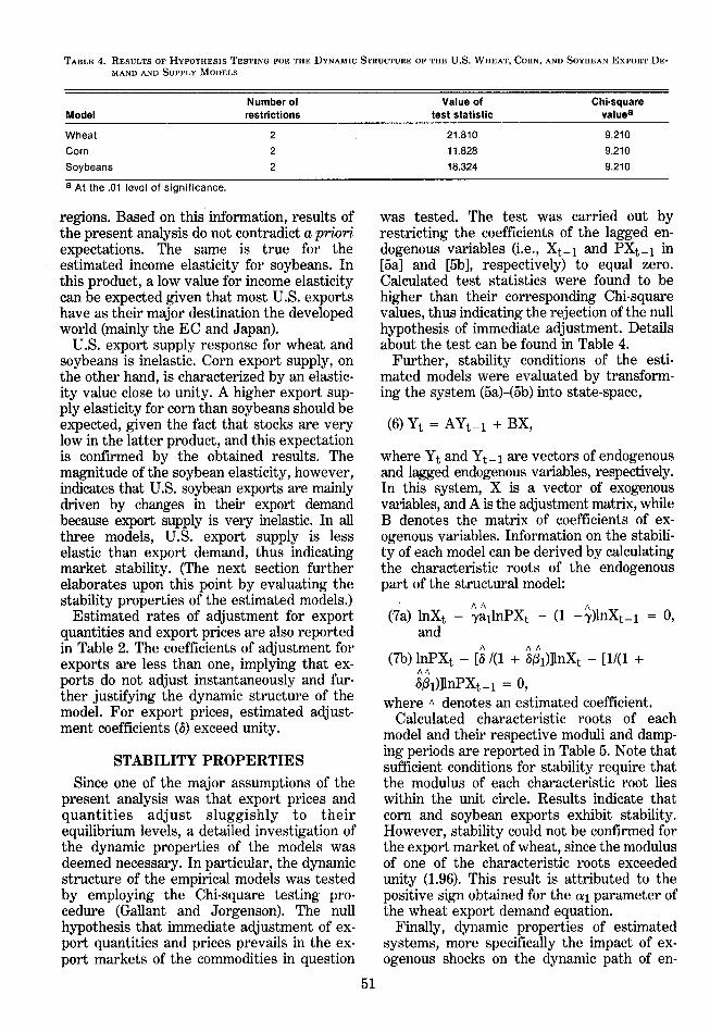
TABLE 4. RESULTS OF HYPOTHESIS TESTING FOR THE DYNAMIC STRUCTURE OF THE U.S. WHEAT, CORN, AND SOYBEAN EXPORT DE-MAND AND SUPPLY MODELS

Number of Value of Chi-squareModel restrictions test statistic valuea

Wheat 2 21.810 9.210Corn 2 11.828 9.210Soybeans 2 18.324 9.210

a At the .01 level of significance.

regions. Based on this information, results of was tested. The test was carried out bythe present analysis do not contradict a priori restricting the coefficients of the lagged en-expectations. The same is true for the dogenous variables (i.e., Xt_ 1 and PXt_1 inestimated income elasticity for soybeans. In [5a] and [5b], respectively) to equal zero.this product, a low value for income elasticity Calculated test statistics were found to becan be expected given that most U.S. exports higher than their corresponding Chi-squarehave as their major destination the developed values, thus indicating the rejection of the nullworld (mainly the EC and Japan). hypothesis of immediate adjustment. Details

U.S. export supply response for wheat and about the test can be found in Table 4.soybeans is inelastic. Corn export supply, on Further, stability conditions of the esti-the other hand, is characterized by an elastic- mated models were evaluated by transform-ity value close to unity. A higher export sup- ing the system (5a)-(5b) into state-space,ply elasticity for corn than soybeans should beexpected, given the fact that stocks are very (6) Yt = AYt_- + BX,low in the latter product, and this expectationis confirmed by the obtained results. The where Yt and Yt-1 are vectors of endogenousmagnitude of the soybean elasticity, however, and lagged endogenous variables, respectively.indicates that U.S. soybean exports are mainly In this system, X is a vector of exogenousdriven by changes in their export demand variables, and A is the adjustment matrix, whilebecause export supply is very inelastic. In all B denotes the matrix of coefficients of ex-three models, U.S. export supply is less ogenous variables. Information on the stabili-elastic than export demand, thus indicating ty of each model can be derived by calculatingmarket stability. (The next section further the characteristic roots of the endogenouselaborates upon this point by evaluating the part of the structural model:stability properties of the estimated models.) ^ ̂

Estimated rates of adjustment for export (7a) lnXt - yallnPXt - (1 -y)lnXt-l = 0,quantities and export prices are also reported andin Table 2. The coefficients of adjustment for A ^ ̂exports are less than one, implying that ex- (7b) PXt -[6 /(1 + )]nXt - [1/(1 +ports do not adjust instantaneously and fur- 6Gl)]lnPXt_l = 0,ther justifying the dynamic structure of the where A denotes an estimated coefficient.model. For export prices, estimated adjust- Calculated characteristic roots of eachment coefficients (6) exceed unity. model and their respective moduli and damp-

STABILITY PROPERTIES ing periods are reported in Table 5. Note thatsufficient conditions for stability require that

Since one of the major assumptions of the the modulus of each characteristic root liespresent analysis was that export prices and within the unit circle. Results indicate thatquantities adjust sluggishly to their corn and soybean exports exhibit stability.equilibrium levels, a detailed investigation of However, stability could not be confirmed forthe dynamic properties of the models was the export market of wheat, since the modulusdeemed necessary. In particular, the dynamic of one of the characteristic roots exceededstructure of the empirical models was tested unity (1.96). This result is attributed to theby employing the Chi-square testing pro- positive sign obtained for the il parameter ofcedure (Gallant and Jorgenson). The null the wheat export demand equation.hypothesis that immediate adjustment of ex- Finally, dynamic properties of estimatedport quantities and prices prevails in the ex- systems, more specifically the impact of ex-port markets of the commodities in question ogenous shocks on the dynamic path of en-

51

TABLE 5. CALCULATED CHARACTERISTIC ROOTS, MODULI, AND DAMPING PERIODS OF ENDOGENOUS VARIABLES' ADJUSTMENTMATRICES FOR U.S. EXPORT DEMAND AND SUPPLY MODELS OF WHEAT, CORN, AND SOYBEANS

Characteristic RootModel Real Part Imaginary Part Modulus Damping Period

Wheat 0.276 0.276 3.6221.956 1.956 0.511

Corn 0.227 ± 0.171i 0.284 3.519Soybeans 0.346 ± 0.215i 0.407 2.455

dogenous variables, were evaluated by meas- tities in all three models. The impact ofuring impact, interim, and total multipliers domestic export capacity (Y) or domestic(Chow). Reported values of multipliers for the prices (P) on U.S. export prices of wheat orestimated models indicate that exogenous unit corn is minimal. Soybeans, on the other hand,shocks in the wheat and corn markets result in indicate a significant response to changes inendogenous variables converging after the domestic export capacity, which is not surpris-first five periods, with the impact of these ing given that they are an intermediate pro-shocks being minimal in most cases (Table 6). duct with domestic crushing an alternative toSoybean export prices exhibit a slower rate of their export.convergence and higher values of totalmultipliers than wheat and corn, but still ex-hibit a stable path of convergence. Ratios of SUMMARY AND CONCLUSIONStotal to interim multipliers, which indicate the The responsiveness of U.S. exports ofimmediate effect of an exogenous shock on an wheat, corn, and soybeans was estimated byendogenous variable, are a little over 20 per- incorporating the simultaneous interaction ofcent in all three models. Increases in world ex- their demand and supply. Results indicateport prices of competitors (PXW) or in income that all three estimated models fitted theof importers (YW) have a greater impact on observed data for the 1966-85 period well.U.S. export prices than on U.S. export quan- Further, these results exhibit important dif-

TABLE 6. ESTIMATED IMPACT, INTERIM, AND TOTAL MULTIPLIERS OF THE WHEAT, CORN, AND SOYBEAN MODELS

Lag in Unit increase in PXW Unit increase in YW Unit increase in Y Unit increase in PYears X PX X PX X PX X PX

Wheat0 0.1799 0.5525 0.2670 0.8200 0.0000 -0.3529 0.0000 -0.22225 0.0021 0.0692 0.0032 0.1027 0.0000 -0.0244 0.0000 -0.0154

10 0.0000 0.0052 0.0000 0.0077 0.0000 -0.0017 0.0000 -0.001115 0.0000 0.0004 0.0000 0.0005 0.0000 -0.0001 0.0000 -0.000119 0.0000 0.0000 0.0000 0.0000 0.0000 -0.0000 0.0000 -0.0000

Total 0.7425 2.2749 1.1020 3.3764 0.0000 -1.4550 0.0000 -0.9160

Corn0 -0.3470 -0.5286 0.3686 0.5615 0.0000 -0.2038 0.0000 -0.05545 -0.0006 -0.0212 0.0006 0.0225 0.0000 -0.0056 0.0000 -0.0015

10 -0.0000 -0.0006 0.0000 0.0006 0.0000 -0.0002 0.0000 -0.000015 -0.0000 -0.0000 0.0000 0.0000 0.0000 -0.0000 0.0000 -0.000019 -0.0000 -0.0000 0.0000 0.0000 0.0000 -0.0000 0.0000 -0.0000

Total -1.7262 -1.8665 1.8337 1.9827 0.0000 -0.8157 0.0000 -0.2218

Soybeans0 -0.1349 -0.6993 0.2462 1.2759 0.0000 -1.0231 0.0000 -0.28975 -0.0007 -0.2434 0.0012 0.4441 0.0000 -0.2858 0.0000 -0.0809

10 -0.0000 -0.0682 0.0000 0.1245 0.0000 -0.0798 0.0000 -0.022615 -0.0000 -0.0191 0.0000 0.0348 0.0000 -0.0223 0.0000 -0.006319 -0.0000 -0.0089 0.0000 0.0162 0.0000 -0.0104 0.0000 -0.0029

Total -0.5955 -4.2399 1.0865 7.7353 0.0000 -5.8644 0.0000 -1.6607

X = Exports, PX = Export Price, PXW = World Export Price, YW = Weighted Importers' Income, Y = Index of Export Capacity, and P = Domestic PriceIndex.

52

ferences in the export behavior of each com- ing export revenues, despite the increase inmodity. Export demand was elastic for corn export volume. Recent trends in soybeans,and inelastic for soybeans, while for wheat the however, indicate lower than normal levels ofderived elasticity of export demand had a stocks and expectations for price increases.positive sign. This problematic result of the Thus, the inelastic price response of soybeanwheat export demand can be attributed to the exports could be expected to generate increasedoligopolistic structure of the world wheat export revenues despite the increasing short-market, which has also hampered efforts to run trend in soybean prices.measure export demand response in previous The inconclusive results of the wheat modelempirical research. Income elasticities of ex- with respect to the U.S. price elasticity of ex-port demand were close to unity for wheat and port demand reflect the strategic behaviorsoybeans, while corn exhibited elastic that characterizes major wheat exporters. Asresponse to income changes in importing long as government interventions areregions. Export supply was elastic for wheat widespread in agricultural trade, wheat canand soybeans and nearly unitary elastic for be expected to be among the commoditiescorn. most affected by policies whose application

Hypothesis testing validated the dynamic implies that non-price considerations are anstructure of estimated models in all markets. important determinant in wheat trade flows.Stability properties were confirmed in export In this respect, the escalating subsidy warmarkets of corn and soybeans, but stability between the U.S. and the EC in world wheatresults were inconclusive for the wheat markets is an indication of the recognition ofmarket. Adjustment coefficients indicate that this reality by the two sides. Such a policy canexports and export prices do not adjust im- certainly create short-run gains in exportmediately to their equilibrium levels. Multi- markets. However, in the long run the impactplier impacts indicate a stable path of con- of the reliance on subsidization for increasedvergence for all markets, with a minimal im- exports for wheat can only be detrimentalpact of exogenous shocks on wheat and corn both for U.S. and EC budgets and for U.S.-ECexports and export prices. Soybean export agricultural trade relations.prices exhibit significant response to changes Second, results indicate that export quan-in domestic export capacity, but minimal tities and prices do not adjust instantaneouslyresponse to other exogenous shocks. to their equilibrium levels. Although all three

Results of this analysis, obtained by em- commodities exhibit a stable path of con-pirically estimating within the same vergence, implied lags in their adjustmentmethodological framework export demand have important implications for policy deci-and supply models of three products with sions. If short-run considerations dominate inquite different market characteristics, sug- domestic farm income decisions, observedgest important policy conclusions concerning delays in the realization of farm policy objec-the appropriate export enhancing policy for tives or the associated costs of adjustmentthese products. First, the different export may lead to policy reversals that could haveprice responsiveness of each product implies been avoided if the lags in these adjustmentsthat the rather uniform decline of U.S. farm had been explicitly recognized. Thus, thereexports in the first half of the 1980s cannot be may not be an immediate adjustment to policyreversed with the use of uniform policies for changes contained in the Food Security Act ofeach agricultural product. 1985, but the effects in the export market may

Elastic price response for corn export de- be evident before the expiration of the legis-mand indicates that lowering its loan rate ation.would have a significant impact in increasing Finally, estimation of models for U.S. com-the volume and value of U.S. corn exports. petitors for the same products would provideThis conclusion is consistent with recent better understanding of the complex interac-trends in U.S. corn exports and provides a tions in export markets. Data limitationclear indication that the loan rate decreases prevented the extension of this analysis to in-implemented by the 1985 Farm Bill were in elude behavior of U.S. competitors. However,the right direction for this specific commodity. the estimated models for U.S. wheat, corn,U.S. soybean export response, on the other and soybean exports provide usefulhand, is not elastic. Consequently, a drop in methodological conclusions that can be util-U.S. soybean prices would result in decreas- ized in further trade policy research.

53

REFERENCESAbbott, P. C. "Estimating U.S. Agricultural Export Demand Elasticities: Econometric and

Economic Issues." Paper presented at the IATRC Analytical Symposium on "Elasticitiesin International Agricultural Trade," Dearborn, MI, July 30-August 1, 1987.

Bredahl, M. E., W. H. Meyers, and K. J. Collins. "The Elasticity of Foreign Demand for U.S.Agricultural Products: The Importance of the Price Transmission Elasticity." Amer. J.Agr. Econ., 61(1979):58-63.

Chow, G. C. Analysis and Control of Dynamic Economic Systems. New York: John Wiley &Sons, 1975.

Davison, C. W., and C. A. Arnade. "Export Elasticities for U.S. Soybeans: Estimation Alter-natives." Selected paper presented at the SAEA annual meeting, New Orleans, LA,February 1-3, 1988.

Durbin, J, "Testing for Serial Correlation in Least-Squares Regression When Some of theRegressors are Lagged Dependent Variables." Econometrica, 38(1970):410-21.

Dutton, J., and T. Grennes. "Alternative Measures of Effective Exchange Rates forAgricultural Trade." Eur. Rev. Agr. Econ., 14(1988):427-42.

Figueroa, E., and A. Webb. "An Analysis of the U.S. Grain Embargo Using a QuarterlyArmington-type Model." Embargoes, Surplus Disposal, and U.S. Agriculture.Washington, DC: U.S. Department of Agriculture Staff Report No. AGES860910,Economic Research Service, November 1986.

Food and Agriculture Organization of the United Nations. FAO Trade Yearbook. Rome.Selected years.

Freebairn, J. W., G. C. Rausser, and H. de Gorter. "Monetary Policy and U.S. Agriculture."International Agricultural Trade. Ed. G. C. Storey, A. Schmitz, and A. H. Sarris.Boulder: Westview Press, 1984.

Gallant, A. R., and D. W. Jorgenson. "Statistical Inference for a System of Simultaneous,Nonlinear, Implicit Equations in the Context of Instrumental Variables Estimation."J. Econometrics, 119(1979): 275-302.

Gardiner, W. H., and P.M.M Dixit. "Price Elasticity of Export Demand: Concepts andEstimates." Foreign Agricultural Economic Report No. 228, IED/ERS/USDA. Washing-ton, DC: February 1987.

Gilmour, B., and P. Fawcett. "The Relationship between U.S. and Canadian Wheat Prices."Canadian J. Agr. Econ., 35(1987):571-89.

Goldstein, M., and M. S. Khan. "The Supply and Demand for Exports: A Simultaneous Ap-proach." Rev. Econ. & Stat., 60(1978):275-86.

"Income and Price Effects in Foreign Trade." Handbook of InternationalEconomics. Ed. R.W. Jones and P.B. Kenen. Amsterdam: North-Holland, 1984.

Houthakker, H. S., and S. P. Magee. "Income and Price Elasticities in World Trade." Rev.Econ. & Stat., 51(1969):111-25.

International Monetary Fund. International Financial Statistics, Yearbook of 1985.Washington, DC, 1985.

Meyers, W. H., S. Devadoss, and M. D. Helmar. "Agricultural Trade Liberalization: Cross-Commodity and Cross-Country Impact Products." J. Policy Modeling, 9(1987):455-82.

Miller, S. E., 0. Capps, and G. J. Wells. "Confidence Intervals for Elasticities and Flexibilitiesfrom Linear Equations." Amer. J. Agr. Econ., 66(1984):392-96.

Orcutt, G. "Measurement of Price Elasticities in International Trade." Rev. Econ. & Stat.,32(1950):117-32.

Orden, D. "Agriculture, Trade, and Macroeconomics: The U.S. Case." J. Policy Modeling, 8(1986):27-51.Paarlberg, P. L., and P. C. Abbott. "Oligopolistic Behavior by Public Agencies in International

Trade: The World Wheat Market." Amer. J. Agr. Econ., 68(1986):528-42.Paarlberg, P. L., A. J. Webb, A. Morey, and J. A. Sharples. "Impacts of Policy on U.S.

Agricultural Trade." ERS Staff Report No. AGES840802, IED/ERS/USDA. Washing-ton, DC: December 1984.

54

Rausser, G. C. "Macroeconomics and U.S. Agricultural Policy." U.S. Agricultural Policy. Ed.B. Gardner. Washington, DC: American Enterprise Institute, 1985.

Rausser, G. C., J. A. Chalfant, H. A. Love, and K. G. Stamoulis. "Macroeconomic Linkages,Taxes, and Subsidies in the U.S. Agricultural Sector." Amer. J. Agr. Econ.,68(1986):399-412.

Sargan, J. D. "Some Discrete Approximations to Continuous Time Stochastic Models."J. Royal Stat. Soc., 34 Series B(1975):74-90.

Sarris, A. H., and J. Freebairn. "Endogenous Price Policies and International Wheat Prices."Amer. J. Agr. Econ. 65(1983):214-24.

Schmitz, A., A. F. McCalla, D. 0. Mitchell, and C. A. Carter. Grain Export Cartels. Cam-bridge, Mass.: Ballinger, 1981.

United Nations, Statistical Office. Commodity Trade Statistics. New York. Selected years.United States Congress, Office of Technology Assessment. A Review of U.S. Competitiveness

in Agricultural Trade-A Technical Memorandum. OTA-TM-TET 29. Washington, DC:U.S. Government Printing Office, 1986.

United States Department of Agriculture, Economic Research Service. Foreign AgriculturalTrade of the United States, Calendar Year Supplements, selected years.

. Unpublished supply utilization tables for wheat, corn, and soybeans.

. Foreign Agriculture Service. Foreign Agricultural Circular: Oilseeds and Prod-ucts, selected issues.

55

56