The derivation of Load Enhancement Factors for life …emits.sso.esa.int/emits-doc/ESTEC/8042_RD48FinalReportV...APPENDIX II : Life factor and Load enhancement factor derivation.....162

Prepared by VIX Emmanuelle

Reference TEC-MSS/2010/128/ln/EV Issue 1 Revision - Date of Issue 30/07/2010 Status N/A Document Type STU Distribution ESA, IfMA

ESA UNCLASSIFIED – For Official Use

Final report Vix 2010.doc


estec

European Space Research and Technology Centre

Keplerlaan 1 2201 AZ Noordwijk

The Netherlands T +31 (0)71 565 6565 F +31 (0)71 565 6040

www.esa.int

Final Report The derivation of Load Enhancement Factors for life testing of composites.

Page 2/181

Derivation of LEF for life testing composites

Date 30/07/2010 Issue 1 Rev -



Title The derivation of Load Enhancement Factors for life testing of composites

Issue 1 Revision -

Author Emmanuelle VIX Date 30/07/2010

Reviewed by Gerben SINNEMA Date 30/07/2010

Approved by Rafael BUREO DACAL Date 30/07/2010

Reason for change Issue Revision Date

Issue 1 Revision -

Reason for change Date Pages Paragraph(s)

Page 3/181





Table of contents:

Abstract....................................................................................................................................................7 1 Introduction .................................................................................................................................... 10 1.1 Differences between metals and composites ..................................................................................................................10 1.2 The life factor approach ................................................................................................................................................... 15 1.2.1 General approach........................................................................................................................................................... 15 1.2.2 Life factor definition...................................................................................................................................................... 16 1.2.3 Examples of life factors ................................................................................................................................................. 16 1.3 The LEF approach............................................................................................................................................................ 18 2 Composites certification ..................................................................................................................20 2.1 Building block approach ................................................................................................................................................. 20 2.1.1 Philosophy of the building block approach ................................................................................................................. 20 2.2 Building block levels ........................................................................................................................................................22 2.2.1 Group A: material property development ....................................................................................................................22 2.2.1.1 Block 1: material screening and selection..................................................................................................................22 2.2.1.2 Block 2: material and process specification development ........................................................................................23 2.2.1.3 Block 3: Allowable development ................................................................................................................................23 2.2.1.3.1 A-basis values..........................................................................................................................................................23 2.2.1.3.2 B-basis values .........................................................................................................................................................23 2.2.2 Groups B: Design-value development ..........................................................................................................................24 2.2.2.1 Block 4: structural element tests............................................................................................................................... 24 2.2.2.2 Block 5: subcomponents tests ................................................................................................................................... 24 2.2.3 Group C: Analysis verification ......................................................................................................................................24 2.2.3.1 Block 6: component test ............................................................................................................................................ 24 2.3 Example of the Boeing 777 empennage structure certification approach .....................................................................25 2.3.1 Certification approach...................................................................................................................................................26 2.3.2 Development test program............................................................................................................................................27 2.3.2.1 Preproduction horizontal stabilizer Test ...................................................................................................................27 2.3.2.2 Vertical stabilizer root attachment............................................................................................................................ 28 2.3.2.3 Subcomponents tests................................................................................................................................................. 28 2.3.2.4 Coupons and Elements tests ..................................................................................................................................... 29 2.3.3 Production component tests .........................................................................................................................................29 2.3.3.1 777 horizontal stabilizer test...................................................................................................................................... 29 2.3.3.2 777Vertical stabilizer ................................................................................................................................................. 29 3 Testing methods .............................................................................................................................. 31 3.1 Fiber testing ..................................................................................................................................................................... 31 3.1.1 Filament tensile testing ................................................................................................................................................. 31 3.1.2 Tow tensile testing .........................................................................................................................................................32 3.2 Matrix testing (MIL HDBK 17 Vol 1) ...............................................................................................................................33 3.2.1 Static mechanical properties testing.............................................................................................................................33 3.2.2 Fatigue testing................................................................................................................................................................34 3.3 Lamina and laminate testing (MIL hdbk 17 vol 1 and ASM hdbk vol 21) ......................................................................34 3.3.1 Example of test matrix ..................................................................................................................................................34 3.3.2. Tensile property test methods (MIL hdbk) ..................................................................................................................35 3.3.3. Compressive property test methods (ASM hdbk Vol 21) .............................................................................................37 3.3.4. Shear property test methods .........................................................................................................................................39 3.4 Impact damage testing.................................................................................................................................................... 40

Page 4/181





3.4.1. Example of impact test specimen ................................................................................................................................ 40 3.4.2. Impact test apparatus.................................................................................................................................................... 41 3.5 Structural element testing ...............................................................................................................................................45 3.5.1 Notched laminate tests ..................................................................................................................................................45 3.5.2 Mechanically fastened joint tests ..................................................................................................................................47 3.5.2.1 Bearing tests................................................................................................................................................................47 3.5.2.2 Bearing/by-pass......................................................................................................................................................... 49 3.5.2.3 Shear-out..................................................................................................................................................................... 51 3.5.2.4 Fastener pull-thru strength ........................................................................................................................................ 51 3.5.3 Bonded joints .................................................................................................................................................................52 3.5.3.1 Adhesive ......................................................................................................................................................................52 3.5.3.2 Bonded ........................................................................................................................................................................53 3.6 Examples of testing approaches already used ................................................................................................................57 3.6.1 NASA Coupon testing requirements.............................................................................................................................57 3.6.2. EADS Casa testing .........................................................................................................................................................58 3.6.3. Raytheon Jet plane test matrix ..................................................................................................................................... 61 3.6.4. Impact testing from FAA............................................................................................................................................... 61 3.6.5. Waruna PhD report .......................................................................................................................................................63 4 Mathematical methods of scatter analysis: the so-called “data pooling techniques”........................65 4.1 The Weibull analysis ........................................................................................................................................................65 4.1.1 Individual Weibull method ...........................................................................................................................................65 4.1.2 Joint Weibull method....................................................................................................................................................66 4.2 The Sendeckyj analysis ....................................................................................................................................................67 4.2.1 Nature of Fatigue Data ..................................................................................................................................................67 4.2.2 Definitions..................................................................................................................................................................... 68 4.2.3 The wearout model ....................................................................................................................................................... 68 4.2.4 Method to obtain fatigue model parameters of the wearout model ............................................................................ 71 4.2.5 Maximum likelihood estimators ...................................................................................................................................72 4.2.6 The Sendeckyj data-fitting procedure...........................................................................................................................73 4.3 Comparison of the different data-pooling techniques....................................................................................................75 4.3.1 Comparison of the results given by each method.........................................................................................................75 4.3.1.1 Description of the material systems...........................................................................................................................75 4.3.1.2 Results.........................................................................................................................................................................76 4.3.2 Conclusions....................................................................................................................................................................78 5 Effect of damage on life and strength scatter ...................................................................................79 5.1 Damage in composites .....................................................................................................................................................79 5.2 Damage tolerance: different control approaches ...........................................................................................................79 5.3 Impact damage................................................................................................................................................................ 80 5.3.1 Sources of impact damage............................................................................................................................................ 80 5.3.2 Parameters of impact damage...................................................................................................................................... 80 5.3.3 Mechanism of an impact damage ................................................................................................................................ 80 5.3.4 Effect of damage on life scatter .................................................................................................................................... 83 5.3.4.1 Description of the data sets ....................................................................................................................................... 83 5.3.4.2 Results........................................................................................................................................................................ 83 5.3.4.3 Conclusions ................................................................................................................................................................ 83 5.3.5 Effect of damage on strength scatter ............................................................................................................................85 5.3.5.1 Results given by Whitehead: post-impact compression strength scatter ................................................................85 5.3.5.2 Results given by Waruna Severinate: static strength data scatter analysis............................................................. 86 5.3.5.3 Conclusions .................................................................................................................................................................87

Page 5/181





6 LEF: overview of the current industrial values and their derivation ............................................... 88 6.1 Load enhancement factor derivation ............................................................................................................................. 88 6.1.1 Computation of LEF values.......................................................................................................................................... 88 6.1.2 LEF values in aircraft industries .................................................................................................................................. 90 6.1.3 Discussion about relevant alpha values ........................................................................................................................ 91 6.2 Sensitivity of the LEF to its parameters ..........................................................................................................................92 6.2.1 Effect of a disturbance of the parameters on the LEF value ........................................................................................92 6.2.2 LEF 3D-plot ...................................................................................................................................................................93 6.3 Extreme case of testing ....................................................................................................................................................93 7 Assessment of maximum allowed material scatter ..........................................................................95 7.1 General approach .............................................................................................................................................................95 7.2 Basic requirements ..........................................................................................................................................................95 7.3 More considerations ........................................................................................................................................................99 8 Considerations for choosing a LEF default value ........................................................................... 105 8.1 Probabilistic background...............................................................................................................................................105 8.1.1 General reliability problem .........................................................................................................................................105 8.1.2 Monte Carlo Simulation Method ................................................................................................................................105 8.2 Finite Element Reliability Using Matlab (FERUM) ..................................................................................................... 107 8.3 Reliability analysis: choosing a LEF default value........................................................................................................ 107 8.3.1 Definition of the problem............................................................................................................................................ 107 8.3.1.1 Deterministic variables............................................................................................................................................. 107 8.3.1.2 Random variables ..................................................................................................................................................... 107 8.3.1.3 The limit state function ............................................................................................................................................109 8.3.1.4 Simulated random variables ....................................................................................................................................109 8.3.2 Results..........................................................................................................................................................................109 8.3.2.1 Effect of the LEF default value and of the test duration in lifetimes......................................................................109 8.3.2.2 Effect of correlation between life and strength shape parameters ......................................................................... 112 8.3.2.2.1 Definitions ............................................................................................................................................................ 112 8.3.2.2.2 Effect of correlation on Pf.................................................................................................................................... 113 8.3.2.3 A-basis values vs B-basis values............................................................................................................................... 116 8.4 Interpretations discussions and conclusions................................................................................................................ 118 9 Waruna’s data nalysis.....................................................................................................................119 9.1 Available data ................................................................................................................................................................. 119 9.2 Easyfit software .............................................................................................................................................................. 119 9.3 Statistical analysis .......................................................................................................................................................... 119 9.3.1 Strength data................................................................................................................................................................ 119 9.3.2 Fatigue data.................................................................................................................................................................. 121 9.3.3 Correlation between life and strength shape parameters .......................................................................................... 122 9.4 Distributions fitting for strength and fatigue life ......................................................................................................... 124 9.4.1 Strenght data fiting...................................................................................................................................................... 124 9.4.2 Fatigue life data fitting ................................................................................................................................................ 129 9.5 Distributions fitting for alpha L and alpha R................................................................................................................ 133 9.6 Conclusions .................................................................................................................................................................... 141 10 Other tools for full scale testing ..................................................................................................... 142 10.1 The use of safety and proof factors for full scale testing .............................................................................................. 142 10.1.1 Safety factors................................................................................................................................................................ 142 10.1.2 Proof test ...................................................................................................................................................................... 142 10.1.3 Overview or safety and proof factors required for space certification....................................................................... 143 10.2 The use of Spectrum truncation for component and full scale testing ........................................................................ 145

Page 6/181





10.2.1 State-of-the-art ............................................................................................................................................................ 145 10.2.2 Results of J.SCHÖN spectrum truncation testing......................................................................................................146 10.2.2.1 Tests achieved with the vertical tail fighter aircraft spectrum: the bfkb spectrum ...............................................146 10.2.2.1.1 Spectrum description..........................................................................................................................................146 10.2.2.1.2 First type of test specimens................................................................................................................................ 147 10.2.2.1.3 Results for the first type of specimens...............................................................................................................148 10.2.2.1.4 Second type of test specimens............................................................................................................................148 10.2.2.1.5 Results for the second type of specimens ..........................................................................................................149 10.2.2.2 Tests achieved with the fighter aircraft wing spectrum: the ofkb spectrum ..........................................................149 10.2.2.2.1 Test Specimens ...................................................................................................................................................150 10.2.2.2.2 Results ................................................................................................................................................................150 10.2.2.3 Specially designed load sequences............................................................................................................................151 10.2.2.3.1 Spectrum description ..........................................................................................................................................151 10.2.2.3.2 Test specimens ................................................................................................................................................... 152 10.2.2.3.3 Results ................................................................................................................................................................ 152 10.2.2.4 Conclusions ............................................................................................................................................................... 152 Conclusions .......................................................................................................................................... 153 References............................................................................................................................................ 155 APPENDIX I : Mathematical backgrounds ...........................................................................................................................158 The Weibull Distribution ........................................................................................................................................................ 158 The Chi-square distribution property: ................................................................................................................................... 159

Determination of and for data set : Maximum likelihood estimation.......................................................................... 159 APPENDIX II : Life factor and Load enhancement factor derivation...................................................................................162 Life factor................................................................................................................................................................................. 162 Load enhancement factor........................................................................................................................................................ 163 APPENDIX III : gamma function, derivation manipulation and equivalent of the function .............................................166 Definition of the function........................................................................................................................................................166 Main properties .......................................................................................................................................................................166 Computing values of the gamma function.............................................................................................................................. 167 APPENDIX IV : FERUM: inputfile_lef.................................................................................................................................169 APPENDIX V: Waruna’s test results and S-N plots...............................................................................................................171

Page 7/181





ABSTRACT

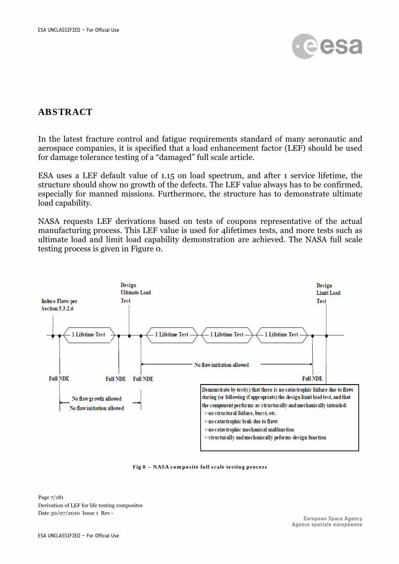
In the latest fracture control and fatigue requirements standard of many aeronautic and aerospace companies, it is specified that a load enhancement factor (LEF) should be used for damage tolerance testing of a “damaged” full scale article. ESA uses a LEF default value of 1.15 on load spectrum, and after 1 service lifetime, the structure should show no growth of the defects. The LEF value always has to be confirmed, especially for manned missions. Furthermore, the structure has to demonstrate ultimate load capability. NASA requests LEF derivations based on tests of coupons representative of the actual manufacturing process. This LEF value is used for 4lifetimes tests, and more tests such as ultimate load and limit load capability demonstration are achieved. The NASA full scale testing process is given in Figure 0.

Fig 0 – NASA composite full scale testing process

Page 8/181





Discussions are still ongoing on updating the standards and investigations are needed about the LEF topic. The objectives of the current study are the following: The study of available literature concerning LEF definition and derivation The summary of LEF examples applied in actual structural tests, based on literature

review. Make an example how LEF could be derived for spacecraft structures (type and number

of samples, calculation of LEF). Identify weather the LEF definition contains (implicit) assumptions that may be more

suitable for aircraft than for typical spacecraft applications. Identify whether significantly different scatter in life is observed for “undamaged”

composites than for “damaged” composites What tests on coupons are needed to compute available LEF values or at least to

demonstrate a maximum scatter? The study of other methods to reduce the testing times for full scale testing (for instance

spectrum truncation) The first chapter of this report is an introduction to the LEF subject and explains why and how it was created. The second chapter describes how composites are certified today for airplane structures, using the building block approach. Chapter 3 is dedicated to a review of test methods that can be applied for different levels of the building block approach. It is shown that the LEF values depend on the scatter in life and strength. Chapter 4 gives mathematical methods to derive these two parameters. During full scale testing, structures which are tested are damaged structures. This is because experience showed that impact damage and many damage are important issue for composite materials. The aim of chapter 5 is to try to assess whether damage and especially impact damage have an influence on the scatter in life and in strength and hence, on the LEF values. Chapter 6 is focused on LEF itself: it addresses the values used during past certification programs, examples of calculations, the influence of the LEF value to each one of its parameters. Chapter 7 investigates an alternative approach for composite certification, in which the material would have to show its reliability in order to justify a default LEF value. In chapter 8 some reliability analysis are performed to know if the LEF value chosen is high enough or not to achieve a certain level of reliability. This was done in support of ongoing discussions on selection of default LEF

Page 9/181





Detailed data of fatigue and strength tests reported by Waruna Severinate (ref [6]) were analysed in chapter 9 with the objective to assess the goodness of the achievec fits for Weibull parameters alpha and beta for which widely varying values are reported, which significantly affects resulting LEF values. In chapter 10, other methods for reducing testing time and effort are described. Safety and proof factors are defined and an overview of the commonly used values for space structure verification is given. Then, studies about the effect of spectrum truncation on composite behaviour in fatigue are given, and a few examples of spectrum truncation for former aircraft certification programs are given.

Page 10/181





1 INTRODUCTION

1.1 Differences between metals and composites

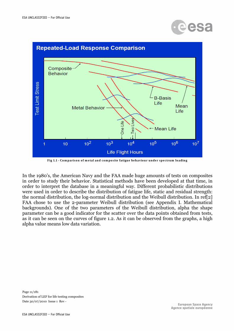
For many years, metals have been used to build structures in many industrial fields (naval, aircrafts, spacecrafts) and many studies have been done to anticipate their behavior in terms of fatigue and fracture. But with the more recent use of materials such as polymers, ceramics or in our case, composites, it is necessary to study their behavior in various situations. If a certification procedure has to be developed on composites, it is first necessary to recognize inherent differences between metals and composites. Metals are known to be sensitive in fatigue to stress concentration, wearers composites are almost not. Unlike metals, composites are multicomponent materials, what means that there can be damage in every component of the material. For metallic materials, damage is usually crack propagation, but for composites, many modes do exist, and all these modes can occur at the same time, what makes the behaviour difficult to anticipate. Damage control for composites is a different approach than fracture control for metals. For composites, the main defects may appear sudden and sometimes remain invisible, and are mechanical damages and manufacturing defects, whereas for metals, defects are based on cracks, which are progressive and gradual damage growth. Conservatism for composites uses ultimate loads and the probability of defect existence for mechanical damage, and the metal conservative approach is based on the probability of defect existence and of the defect severity. For metals, linear elastic fracture mechanics can help to predict the material behaviour, but no analytical tool exists for composite materials. A comparison of the behaviour of metals and composites under an aircraft wing spectrum loading is given in figure 1.1. The results are given in tension dominated loading mode for metals, and compression dominated loading mode for composites, because it is generally their most sensitive loading mode (especially when damaged). As it can be seen on the figure, composite show much higher fatigue properties than metals do. On the other hand, as it can be observed, they show higher scatter in both fatigue life and strength results.

Page 11/181





Fig 1.1 - Comparison of metal and composite fatigue behaviour under spectrum loading

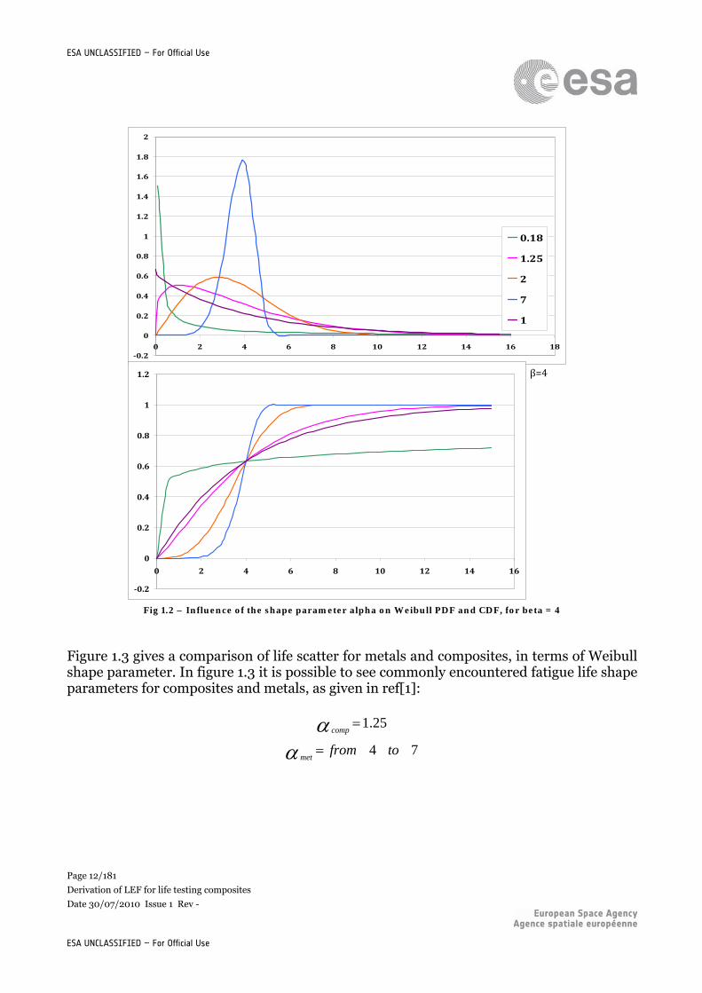
In the 1980’s, the American Navy and the FAA made huge amounts of tests on composites in order to study their behavior. Statistical methods have been developed at that time, in order to interpret the database in a meaningful way. Different probabilistic distributions were used in order to describe the distribution of fatigue life, static and residual strength: the normal distribution, the log-normal distribution and the Weibull distribution. In ref[2] FAA chose to use the 2-parameter Weibull distribution (see Appendix I. Mathematical backgrounds). One of the two parameters of the Weibull distribution, alpha the shape parameter can be a good indicator for the scatter over the data points obtained from tests, as it can be seen on the curves of figure 1.2. As it can be observed from the graphs, a high alpha value means low data variation.

Page 12/181





Fig 1.2 – Influence of the shape parameter alpha on Weibull PDF and CDF, for beta = 4

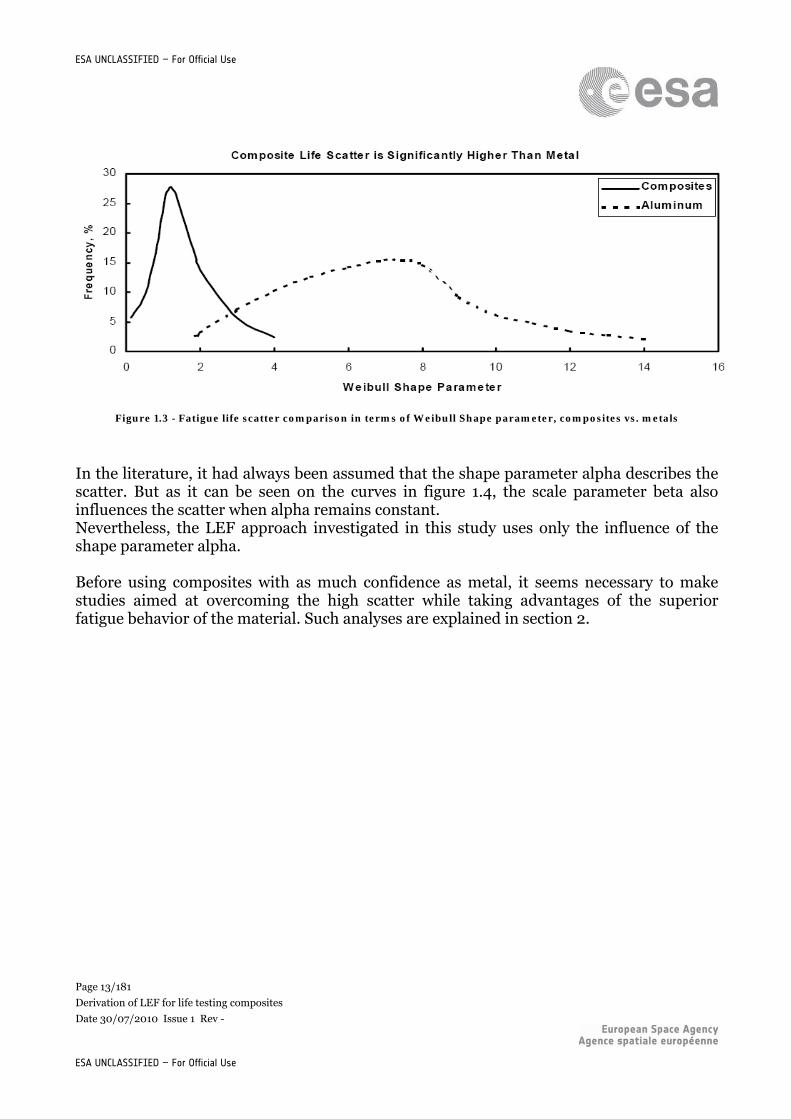
Figure 1.3 gives a comparison of life scatter for metals and composites, in terms of Weibull shape parameter. In figure 1.3 it is possible to see commonly encountered fatigue life shape parameters for composites and metals, as given in ref[1]:

25.1 comp

74 tofrommet

0.2

0

0.2

0.4

0.6

0.8

1

1.2

1.4

1.6

1.8

2

0 2 4 6 8 10 12 14 16 18

0.18

1.25

2

7

1

β=4

0.2

0

0.2

0.4

0.6

0.8

1

1.2

0 2 4 6 8 10 12 14 16

Page 13/181





Figure 1.3 - Fatigue life scatter comparison in terms of Weibull Shape parameter, composites vs. metals

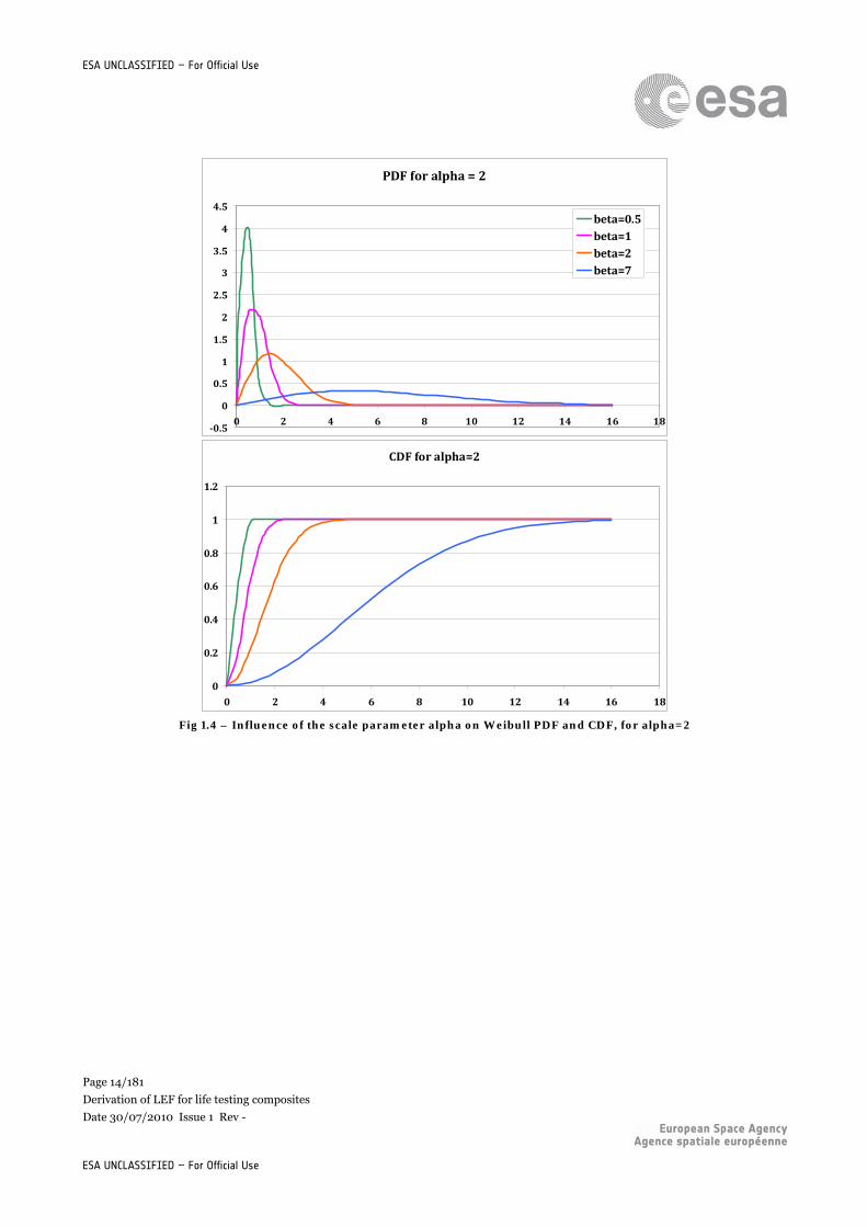
In the literature, it had always been assumed that the shape parameter alpha describes the scatter. But as it can be seen on the curves in figure 1.4, the scale parameter beta also influences the scatter when alpha remains constant. Nevertheless, the LEF approach investigated in this study uses only the influence of the shape parameter alpha. Before using composites with as much confidence as metal, it seems necessary to make studies aimed at overcoming the high scatter while taking advantages of the superior fatigue behavior of the material. Such analyses are explained in section 2.

Page 14/181





Fig 1.4 – Influence of the scale parameter alpha on Weibull PDF and CDF, for alpha=2

PDF for alpha = 2

0.5

0

0.5

1

1.5

2

2.5

3

3.5

4

4.5

0 2 4 6 8 10 12 14 16 18

beta=0.5beta=1beta=2beta=7

CDF for alpha=2

0

0.2

0.4

0.6

0.8

1

1.2

0 2 4 6 8 10 12 14 16 18

Page 15/181





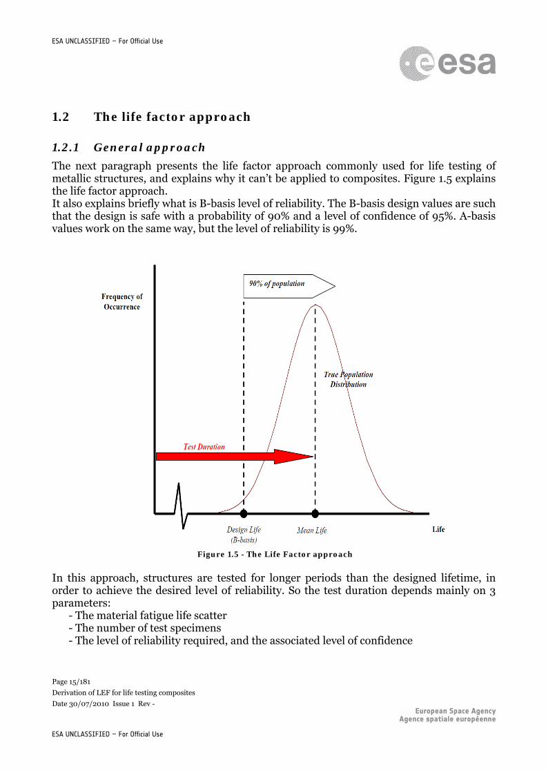
1.2 The life factor approach

1.2.1 General approach

The next paragraph presents the life factor approach commonly used for life testing of metallic structures, and explains why it can’t be applied to composites. Figure 1.5 explains the life factor approach. It also explains briefly what is B-basis level of reliability. The B-basis design values are such that the design is safe with a probability of 90% and a level of confidence of 95%. A-basis values work on the same way, but the level of reliability is 99%.

Figure 1.5 - The Life Factor approach

In this approach, structures are tested for longer periods than the designed lifetime, in order to achieve the desired level of reliability. So the test duration depends mainly on 3 parameters:

- The material fatigue life scatter - The number of test specimens - The level of reliability required, and the associated level of confidence

Page 16/181





1.2.2 Life factor definition

The life factor N f is a multiplicative factor that increases the test duration in order to

improve the reliability for material certification. The derivation of its formula is given in appendix II.

nn

pN

L

L

L

F

22

ln2

1

1

The life factor depends on the fatigue-life shape parameter L, the sampling size n, the

level of reliability p , and the level of confidence γ expected.

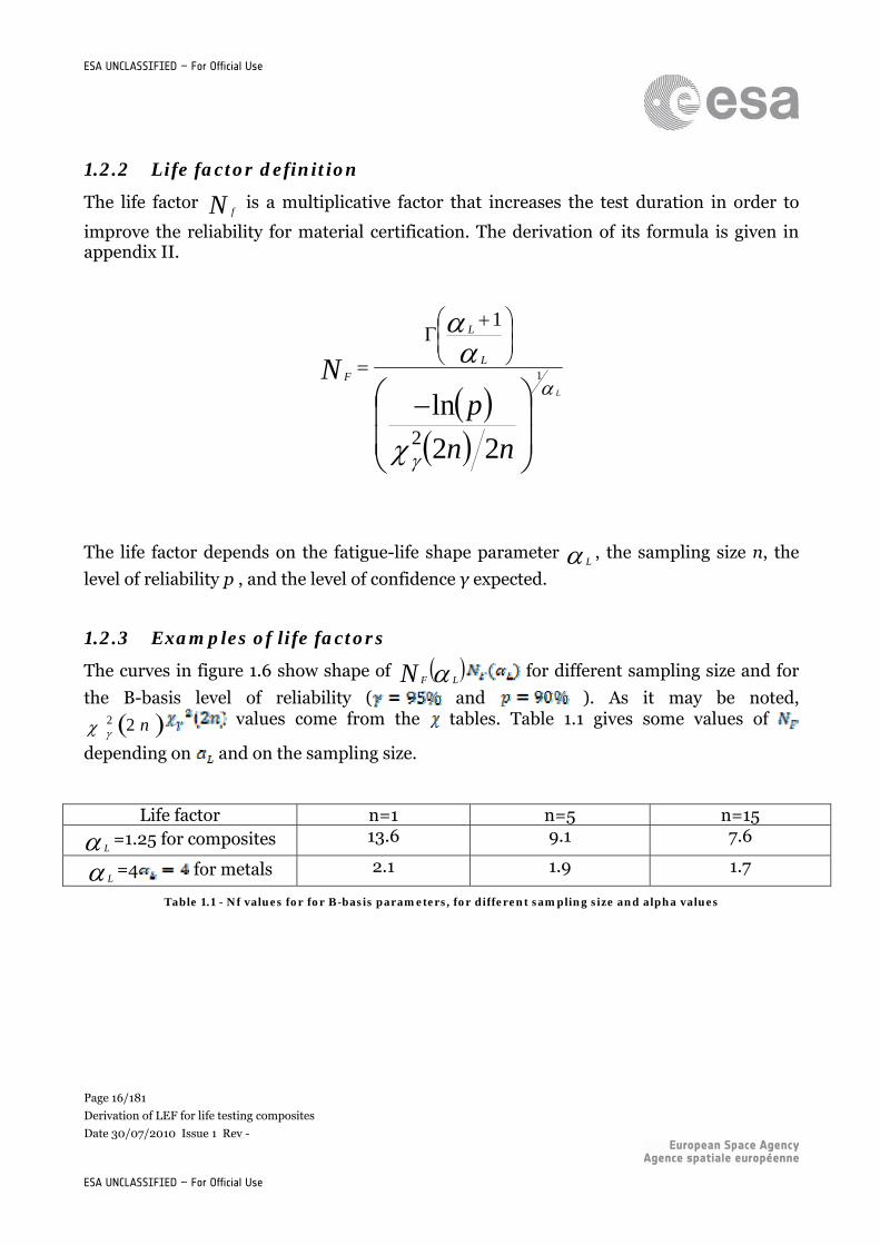
1.2.3 Examples of life factors

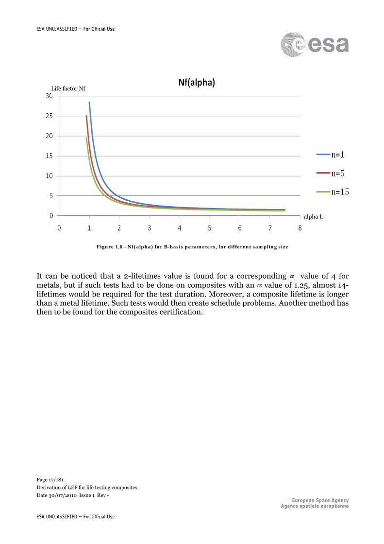
The curves in figure 1.6 show shape of LFN for different sampling size and for

the B-basis level of reliability ( and ). As it may be noted,

n22 values come from the tables. Table 1.1 gives some values of

depending on and on the sampling size.

Life factor n=1 n=5 n=15

L=1.25 for composites 13.6 9.1 7.6

L=4 for metals 2.1 1.9 1.7

Table 1.1 - Nf values for for B-basis parameters, for different sampling size and alpha values

Page 17/181





Figure 1.6 - Nf(alpha) for B-basis parameters, for different sampling size

It can be noticed that a 2-lifetimes value is found for a corresponding value of 4 for metals, but if such tests had to be done on composites with an value of 1.25, almost 14-lifetimes would be required for the test duration. Moreover, a composite lifetime is longer than a metal lifetime. Such tests would then create schedule problems. Another method has then to be found for the composites certification.

alpha L

Life factor Nf

Page 18/181





1.3 The LEF approach

In the certification tests made on metals, structures are tested for 4 lifetimes. Then, if a structure is safe for 4 lifetimes, one can be quite confident about its reliability for 1 lifetime in real conditions. Experience shows that composites generally exhibit superior fatigue properties than metals do. Nevertheless, it has also been observed that composite structures show a higher scatter in both residual strength and fatigue life. Life for structures is commonly represented by a Weibull distribution and as it may be noted, a high value of Weibull shape parameter signifies low data variation. Here are some typical values of the life shape parameters for metals and composites, given in ref [1].

Scatter is much more important for composites lifetime values and if composites had to be tested on the same way as metals do, to achieve the same level of reliability, test duration should last more than 13 lifetimes, what could lead to schedule issues. The load factor approach proposes to increase the load in fatigue certification tests, to have some shorter duration of tests, but while keeping the same level of reliability. LEF is given by the next formula, which is entirely derived in Appendix II.

nnNp L

L

L

LEFR

RL

2)2(

)ln(

1

2

1

With L

the Weibull shape parameter of the fatigue life distribution

R the Weibull shape parameter of the residual strength distribution

n the sampling size (generally 1 for spacecraft structures) N the test duration in lifetimes

p the level of reliability (0.90 for B-basis level of reliability) γ the level of confidence (0.95 for B-basis level of reliability) Γ the gamma function

Page 19/181





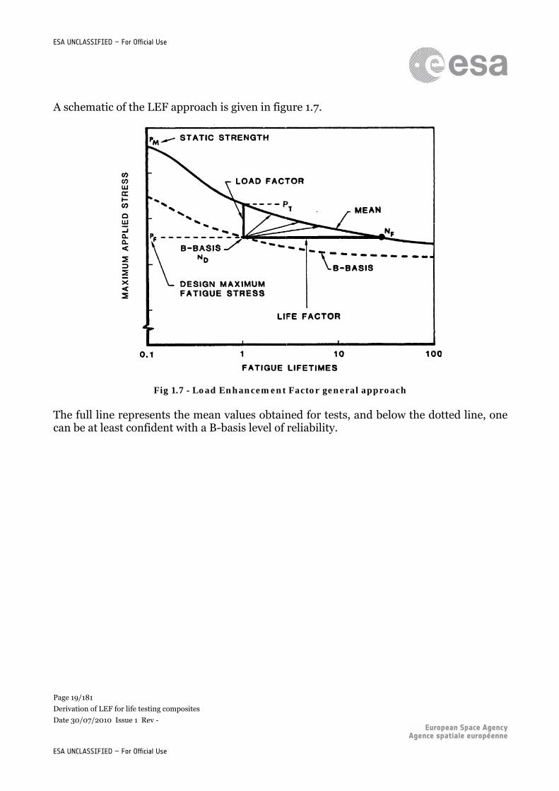
A schematic of the LEF approach is given in figure 1.7.

Fig 1.7 - Load Enhancement Factor general approach The full line represents the mean values obtained for tests, and below the dotted line, one can be at least confident with a B-basis level of reliability.

Page 20/181





2 COMPOSITES CERTIFICATION

If a property is used to verify system capabilities, especially when human safety is involved, testing usually becomes an integral part of the process that is commonly called certification. The engineering of certain critical structures typically follows a specific approval process under the authority of an organization other than the designer. Those approving organization can be for instance the end user, or a government regulatory agency. As said in the introduction, composites and metals are two materials with different behaviours, different properties, and so cannot be certified on the same way. This is the reason why, in this second chapter, the composite certification philosophy is given and then an example of composite structure certification is explained. Most information contained in this section come from ref [1] and ref [19].

2.1 Building block approach

The building block approach described in this section is the method used for airplane structures. It is necessary to study what is done on airplane structures before translating some methods to space structures.

2.1.1 Philosophy of the building block approach

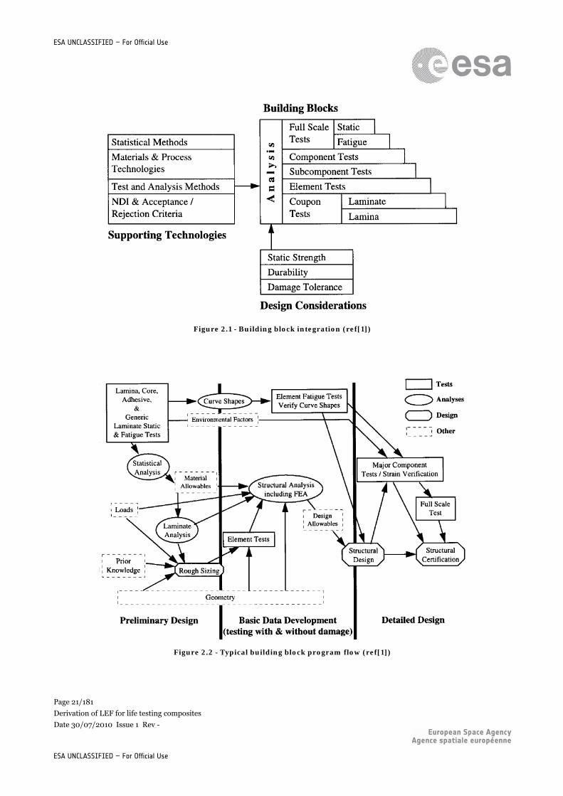
Before using composites to build complex structures, a development program is needed in order to assess the performance of the structure. These programs generally contain various tests and analysis. A high number of tests are needed to achieve a certain level of reliability. This is the reason why testing alone would be too expensive. But using only analysis is not enough to make accurate predictions, since these methods sometimes are not sophisticated enough. The certification programs should therefore be a combination of testing and analysis, in order to reduce costs while increasing the reliability. An extension of this approach mixing tests and analysis is to have some analysis and associated tests at different levels of structural complexity, from small material coupons to full-scale product. Each level is based on what has been learned from previous less complex levels. This substantiation method is called the Building-Block approach. Figure 2.1 gives the Building-Block integration in a certification program, with the help of supporting technologies and while taking into account design considerations. Figure 2.2 represents the flows within the Building-Block certification approach.

Page 21/181





Figure 2.1 - Building block integration (ref[1])

Figure 2.2 - Typical building block program flow (ref[1])

Page 22/181





2.2 Building block levels

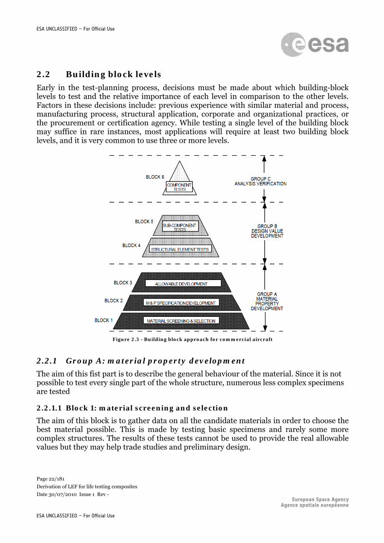
Early in the test-planning process, decisions must be made about which building-block levels to test and the relative importance of each level in comparison to the other levels. Factors in these decisions include: previous experience with similar material and process, manufacturing process, structural application, corporate and organizational practices, or the procurement or certification agency. While testing a single level of the building block may suffice in rare instances, most applications will require at least two building block levels, and it is very common to use three or more levels.

Figure 2.3 - Building block approach for commercial aircraft

2.2.1 Group A: material property development

The aim of this fist part is to describe the general behaviour of the material. Since it is not possible to test every single part of the whole structure, numerous less complex specimens are tested

2.2.1.1 Block 1: material screening and selection

The aim of this block is to gather data on all the candidate materials in order to choose the best material possible. This is made by testing basic specimens and rarely some more complex structures. The results of these tests cannot be used to provide the real allowable values but they may help trade studies and preliminary design.

Page 23/181





2.2.1.2 Block 2: material and process specification development

In this block, the material system needs to be already chosen and prepared. The objective is the validation of the specification and the understanding of the effect of the process variables on the material behaviour. Preliminary qualifications specifications and allowables can be provided but no firm allowable.

2.2.1.3 Block 3: Allowable development

In this block, the material is fully controlled. A material specification and a process specification are needed. The aim here is to provide firm material allowables. Only the data from material purchased and fabricated under strict specifications are accepted. The main objectives of these previous tests are summarized as follows:

- Development of statistically significant data (A and B-basis values) - Determining the effect of environment - Determination of notched effects - Defining changes in properties due to lamination effects - Understanding the effects of manufacturing induced anomalies - Understanding how sensitive the structure is to variations in the fabrication process.

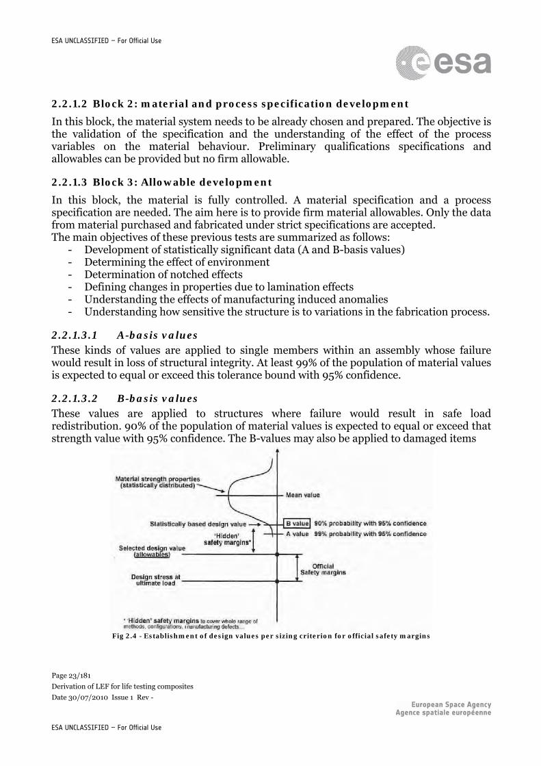
2.2.1.3.1 A-basis values These kinds of values are applied to single members within an assembly whose failure would result in loss of structural integrity. At least 99% of the population of material values is expected to equal or exceed this tolerance bound with 95% confidence.

2.2.1.3.2 B-basis values These values are applied to structures where failure would result in safe load redistribution. 90% of the population of material values is expected to equal or exceed that strength value with 95% confidence. The B-values may also be applied to damaged items

Fig 2.4 - Establishment of design values per sizing criterion for official safety margins

Page 24/181





2.2.2 Groups B: Design-value development

The aim here is to develop design values reflecting the actual structure. Unlike tests of group A, preliminary configurations with general sizing are required. The tests here are very specific and can be used only for one specific kind of structure.

2.2.2.1 Block 4: structural element tests

This block consists in the testing of local structural details repeated within the structure such as bolted joints, stiffener sections, beams and clip flanges, sandwich structures. The main aims are the followings:

- the development of design values that are more related to the structures (and not to the material like in group 1)

- Understanding the effect of manufacturing induced anomalies - Understanding how sensitive the structure is to its fabrication process - Verification of analytical methods to predict structural behaviour of the elements.

2.2.2.2 Block 5: subcomponents tests

This block consists in the testing of more complex components than block 4 (typically sections of a component). These testing are more representative of the real structure and should permit the assessment of load redistribution due to local damage. The tested subcomponents should be of a sufficient size to allow a proper redistribution around flaws and damage. The secondary loading effects, the bending effects, should be represented, and out-of-plane failure modes should become more representative of full-scale-testing. The main objectives are:

- to verify the applicability of the design values and analysis - to verify the effect of damage in static tests - to verify the effect of damage in fatigue tests

2.2.3 Group C: Analysis verification

This is the final stage of the certification process. Extensive verifications of analysis and computer modeling should be performed. The main objectives are the followings:

- The verification of internal loads model and resulting stress strain and deflection predictions.

- A large-scale verification of design analysis methodology

2.2.3.1 Block 6: component test

Here, large and complex full-scale specimen configurations that are representative of the actual structure and its boundary conditions are tested. Test articles in general will contain some degree of credible manufacturing or accidental damage. Generally tests are performed only to design limit load to verify analytical strain and deflection predictions, but some regulatory agencies want the test to be performed until ultimate load or until failure.

Page 25/181





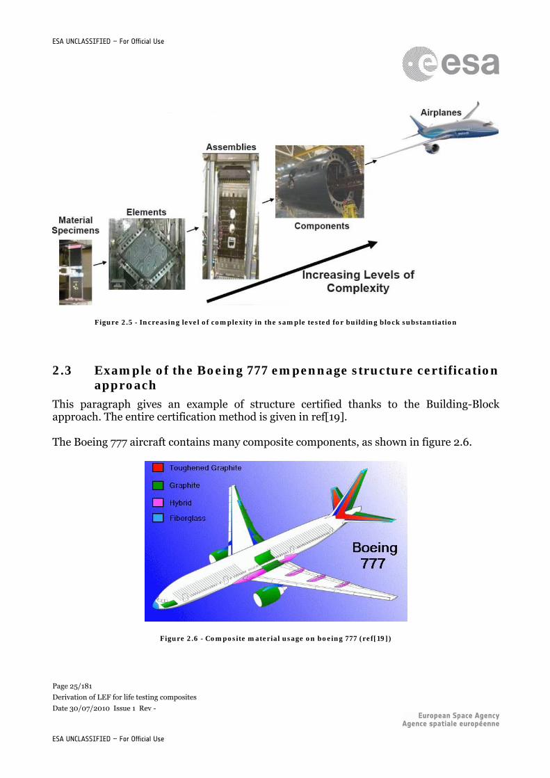
Figure 2.5 - Increasing level of complexity in the sample tested for building block substantiation

2.3 Example of the Boeing 777 empennage structure certification approach

This paragraph gives an example of structure certified thanks to the Building-Block approach. The entire certification method is given in ref[19]. The Boeing 777 aircraft contains many composite components, as shown in figure 2.6.

Figure 2.6 - Composite material usage on boeing 777 (ref[19])

Page 26/181





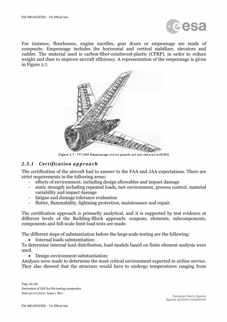
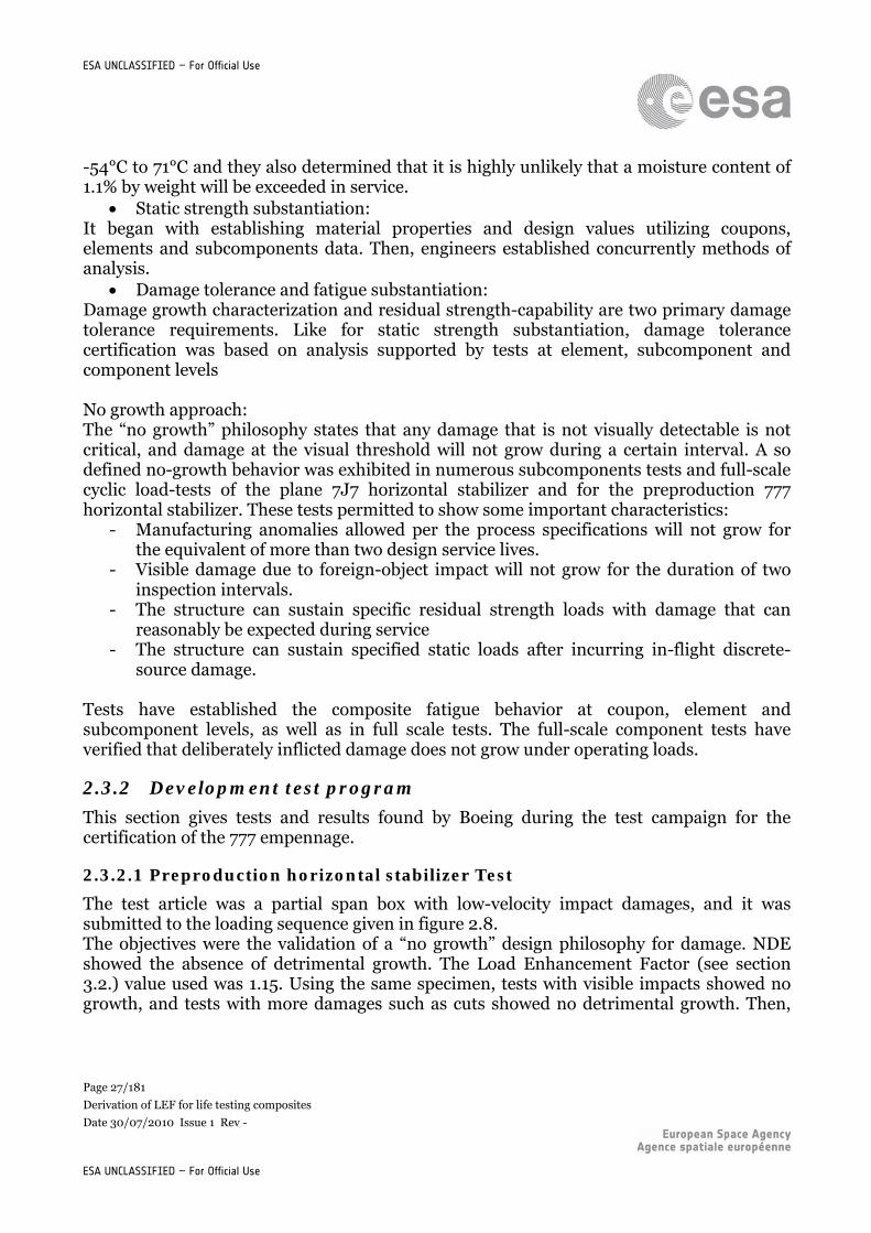
For instance, floorbeams, engine nacelles, gear doors or empennage are made of composite. Empennage includes the horizontal and vertical stabilizer, elevators and rudder. The material used is carbon-fiber-reinforced-plastic (CFRP), in order to reduce weight and then to improve aircraft efficiency. A representation of the empennage is given in Figure 2.7.

Figure 2.7 - 777-200 Empennage (cover panels are not shown) (ref[19])

2.3.1 Certification approach

The certification of the aircraft had to answer to the FAA and JAA expectations. There are strict requirements in the following areas:

- effects of environment, including design allowables and impact damage - static strength including repeated loads, test environment, process control, material

variability and impact damage - fatigue and damage tolerance evaluation - flutter, flammability, lightning protection, maintenance and repair.

The certification approach is primarily analytical, and it is supported by test evidence at different levels of the Building-Block approach: coupons, elements, subcomponents, components and full-scale limit load tests are made. The different steps of substantiation before the large scale testing are the following:

Internal loads substantiation: To determine internal load distribution, load models based on finite element analysis were used.

Design environment substantiation: Analyses were made to determine the most critical environment expected in airline service. They also showed that the structure would have to undergo temperatures ranging from

Page 27/181





-54°C to 71°C and they also determined that it is highly unlikely that a moisture content of 1.1% by weight will be exceeded in service.

Static strength substantiation: It began with establishing material properties and design values utilizing coupons, elements and subcomponents data. Then, engineers established concurrently methods of analysis.

Damage tolerance and fatigue substantiation: Damage growth characterization and residual strength-capability are two primary damage tolerance requirements. Like for static strength substantiation, damage tolerance certification was based on analysis supported by tests at element, subcomponent and component levels No growth approach: The “no growth” philosophy states that any damage that is not visually detectable is not critical, and damage at the visual threshold will not grow during a certain interval. A so defined no-growth behavior was exhibited in numerous subcomponents tests and full-scale cyclic load-tests of the plane 7J7 horizontal stabilizer and for the preproduction 777 horizontal stabilizer. These tests permitted to show some important characteristics:

- Manufacturing anomalies allowed per the process specifications will not grow for the equivalent of more than two design service lives.

- Visible damage due to foreign-object impact will not grow for the duration of two inspection intervals.

- The structure can sustain specific residual strength loads with damage that can reasonably be expected during service

- The structure can sustain specified static loads after incurring in-flight discrete-source damage.

Tests have established the composite fatigue behavior at coupon, element and subcomponent levels, as well as in full scale tests. The full-scale component tests have verified that deliberately inflicted damage does not grow under operating loads.

2.3.2 Development test program

This section gives tests and results found by Boeing during the test campaign for the certification of the 777 empennage.

2.3.2.1 Preproduction horizontal stabilizer Test

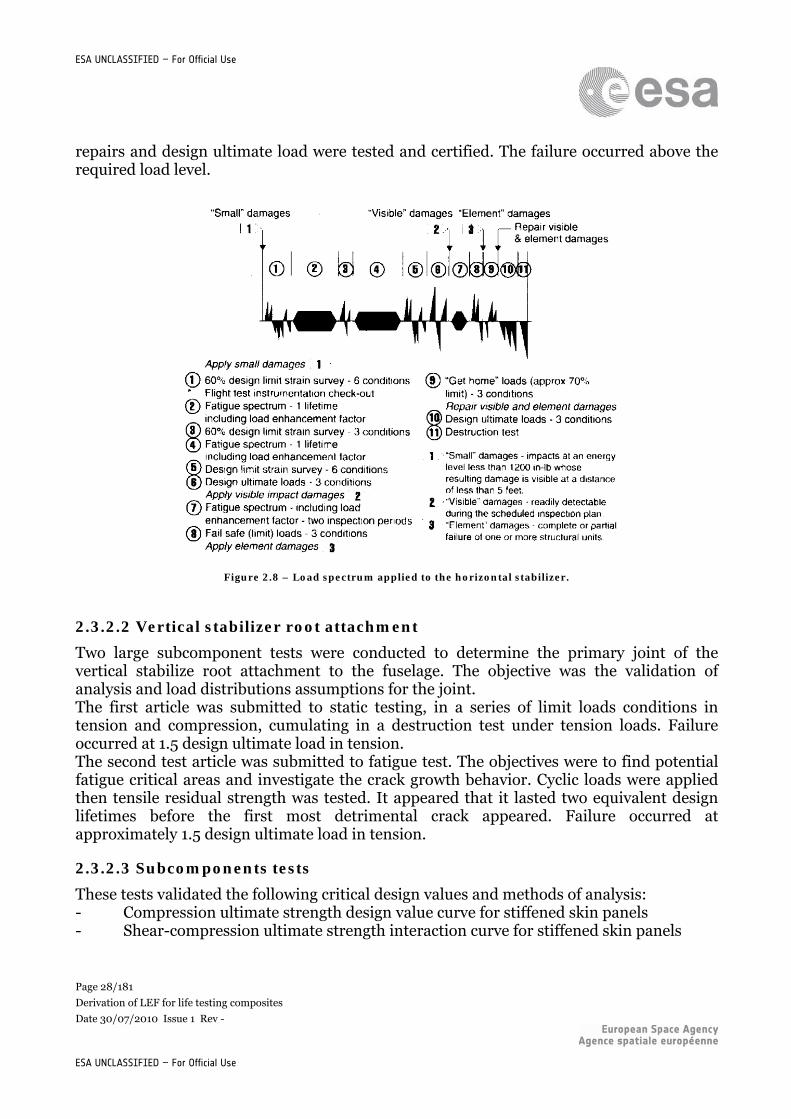
The test article was a partial span box with low-velocity impact damages, and it was submitted to the loading sequence given in figure 2.8. The objectives were the validation of a “no growth” design philosophy for damage. NDE showed the absence of detrimental growth. The Load Enhancement Factor (see section 3.2.) value used was 1.15. Using the same specimen, tests with visible impacts showed no growth, and tests with more damages such as cuts showed no detrimental growth. Then,

Page 28/181





repairs and design ultimate load were tested and certified. The failure occurred above the required load level.

Figure 2.8 – Load spectrum applied to the horizontal stabilizer.

2.3.2.2 Vertical stabilizer root attachment

Two large subcomponent tests were conducted to determine the primary joint of the vertical stabilize root attachment to the fuselage. The objective was the validation of analysis and load distributions assumptions for the joint. The first article was submitted to static testing, in a series of limit loads conditions in tension and compression, cumulating in a destruction test under tension loads. Failure occurred at 1.5 design ultimate load in tension. The second test article was submitted to fatigue test. The objectives were to find potential fatigue critical areas and investigate the crack growth behavior. Cyclic loads were applied then tensile residual strength was tested. It appeared that it lasted two equivalent design lifetimes before the first most detrimental crack appeared. Failure occurred at approximately 1.5 design ultimate load in tension.

2.3.2.3 Subcomponents tests

These tests validated the following critical design values and methods of analysis: - Compression ultimate strength design value curve for stiffened skin panels - Shear-compression ultimate strength interaction curve for stiffened skin panels

Page 29/181





- Compression and tension damage tolerance analysis for stiffened skin panels - Bolted joint analysis and design values for the skin panel-to-trailing edge rib joint - Static compression strength, tension strength, and tension fatigue performance of the horizontal stabilizer centreline splice joint - Analytical methods for spar strain distributions, web stability and peak strains at cut-outs - Analytical methods for rib shear tie and chord strength and stiffness - Peak strain design values for rib shear tie cutouts Also, for small damages, “no growth” was verified, the repair concepts were validate and the shear-compression design envelope was validated.

2.3.2.4 Coupons and Elements tests

These tests established material stiffness properties, statistical allowables, strength design values, and they validated the analytical methods.

2.3.3 Production component tests

This section gives the full-scale production component tests The objectives were the limit load substantiation, and the verification of the load distribution.

2.3.3.1 777 horizontal stabilizer test

This program met the following goals: - To verify the compliance with the expectations established by FAR/JAR. The test

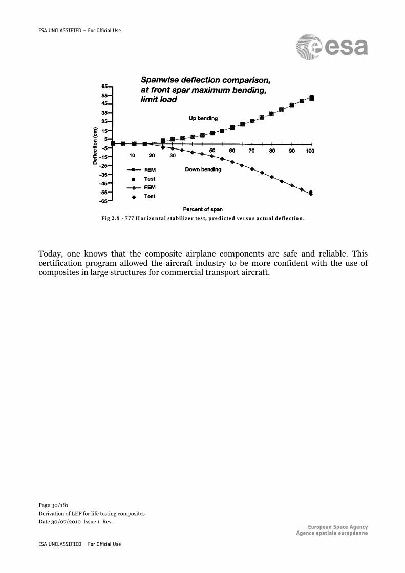
articles sustained limit load for critical conditions without permanent deformations - To verify the predictive capability of analysis methods coupled with subcomponents

tests. Strains and deflection closely matched the analysis as seen figure 1.9. - To verify the design service goals of the structure - To verify the absence of widespread damage due to fatigue.

2.3.3.2 777Vertical stabilizer

Here again, the aim was to show limit load capability and verify the accuracy of analytically calculated strains and deflections. This program met the same goals as those just given for the horizontal stabilizer.

Page 30/181





Fig 2.9 - 777 Horizontal stabilizer test, predicted versus actual deflection.

Today, one knows that the composite airplane components are safe and reliable. This certification program allowed the aircraft industry to be more confident with the use of composites in large structures for commercial transport aircraft.

Page 31/181





3 TESTING METHODS

The building block approach requires a lot of tests at different levels of structural complexity. It can represent more than thousands tests. This chapter is aimed at making a kind of state-of-the-art of the actual testing methods used and recommended.

3.1 Fiber testing

MIL-HDBK 17 Vol 1 gives few trails for fiber testing, for different properties. This paragraph will focus on mechanical properties. All the information next come from the MIL-HDBK 17 Vol 1. Tensile methods are developed and commonly used, but compression methods are still under development and rare. The stress at failure depends on the kind of test performed (tests as filaments, impregnated tow or unidirectional laminate) this is the reason why it is needed to define the objective of fiber testing at the beginning, in order to perform tests representative of the composite behaviour. Carbon fibers are generally tested as impregnated tow, and boron fibers as single filaments.

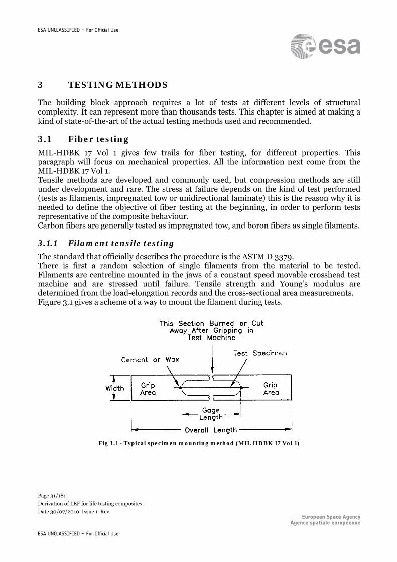
3.1.1 Filament tensile testing

The standard that officially describes the procedure is the ASTM D 3379. There is first a random selection of single filaments from the material to be tested. Filaments are centreline mounted in the jaws of a constant speed movable crosshead test machine and are stressed until failure. Tensile strength and Young’s modulus are determined from the load-elongation records and the cross-sectional area measurements. Figure 3.1 gives a scheme of a way to mount the filament during tests.

Fig 3.1 - Typical specimen mounting method (MIL HDBK 17 Vol 1)

Page 32/181





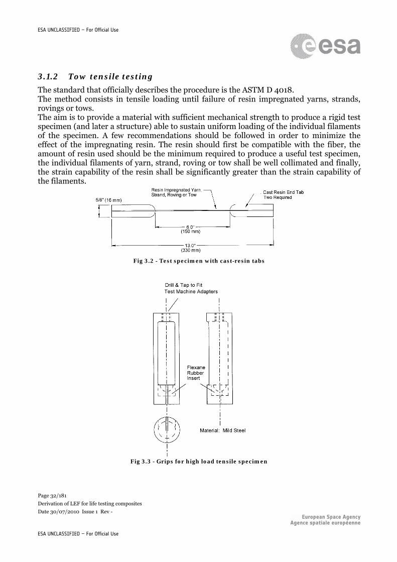
3.1.2 Tow tensile testing

The standard that officially describes the procedure is the ASTM D 4018. The method consists in tensile loading until failure of resin impregnated yarns, strands, rovings or tows. The aim is to provide a material with sufficient mechanical strength to produce a rigid test specimen (and later a structure) able to sustain uniform loading of the individual filaments of the specimen. A few recommendations should be followed in order to minimize the effect of the impregnating resin. The resin should first be compatible with the fiber, the amount of resin used should be the minimum required to produce a useful test specimen, the individual filaments of yarn, strand, roving or tow shall be well collimated and finally, the strain capability of the resin shall be significantly greater than the strain capability of the filaments.

Fig 3.2 - Test specimen with cast-resin tabs

Fig 3.3 - Grips for high load tensile specimen

Page 33/181





3.2 Matrix testing (MIL HDBK 17 Vol 1)

3.2.1 Static mechanical properties testing

Testing the static mechanical properties of the matrix can be an important step. First, it can help to choose a specific material, and then the material can have an impact on one specific property.

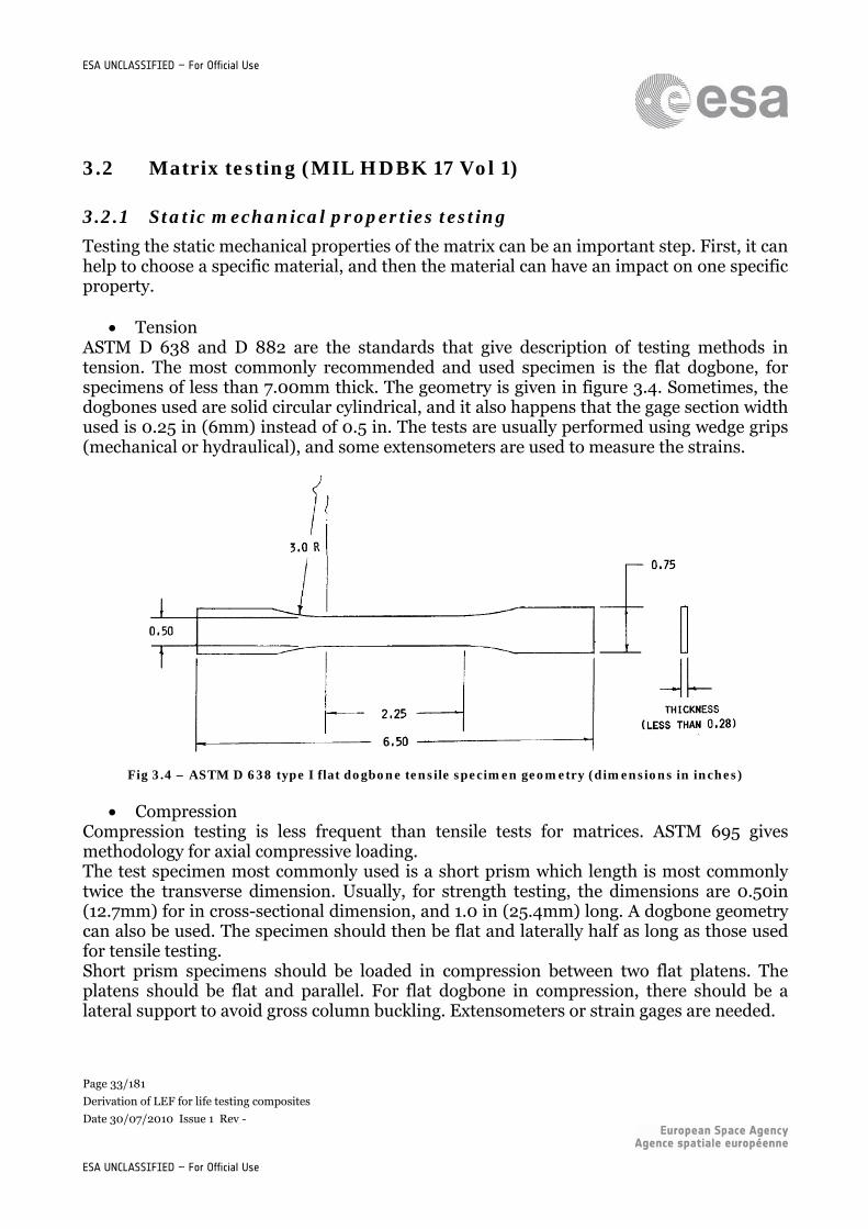
Tension ASTM D 638 and D 882 are the standards that give description of testing methods in tension. The most commonly recommended and used specimen is the flat dogbone, for specimens of less than 7.00mm thick. The geometry is given in figure 3.4. Sometimes, the dogbones used are solid circular cylindrical, and it also happens that the gage section width used is 0.25 in (6mm) instead of 0.5 in. The tests are usually performed using wedge grips (mechanical or hydraulical), and some extensometers are used to measure the strains.

Fig 3.4 – ASTM D 638 type I flat dogbone tensile specimen geometry (dimensions in inches)

Compression Compression testing is less frequent than tensile tests for matrices. ASTM 695 gives methodology for axial compressive loading. The test specimen most commonly used is a short prism which length is most commonly twice the transverse dimension. Usually, for strength testing, the dimensions are 0.50in (12.7mm) for in cross-sectional dimension, and 1.0 in (25.4mm) long. A dogbone geometry can also be used. The specimen should then be flat and laterally half as long as those used for tensile testing. Short prism specimens should be loaded in compression between two flat platens. The platens should be flat and parallel. For flat dogbone in compression, there should be a lateral support to avoid gross column buckling. Extensometers or strain gages are needed.

Page 34/181





Shear ASTM D 5379 and ASTM E 143 describe the method of testing matrix for shear loading mode. The specimens used are solid circular cylinder rods that are loaded in torsion. In general, the geometry is a dogbone cylinder. The standard losipescu (V-notched beam) might also be used. Torsion testing device with low torque capacity for rod, and standard losipescu shear test fixture for losipescu specimens should be used. For both specimens, rosettes on the surface can determine shear modulus and shear stress-strain curve to failure.

Flexure The standard describing the methodology is the ASTM D 790. Specimens are simple rectangular strip of polymer matrix with constant width and thickness. They can be tested either in three-points or in four-point loading.

3.2.2 Fatigue testing

Unreinforced resins should be cyclic loaded to determine the life of the specimens. The tests should be done in various loading conditions such as bending, crack opening, tension, compression, tension/compression reverse, loading, and all the tests should represent different R-ratios. The loading frequencies should be low enough to avoid heating the specimen. For different load amplitudes, many specimens should be tested. The aim is to provide S-N curves.

3.3 Lamina and laminate testing (MIL hdbk 17 vol 1 and ASM hdbk vol 21)

3.3.1 Example of test matrix

MIL-HDBK 17 gives several examples of test matrices recommended for coupon testing, and for different purposes of tests: material screening, material assessment, (…) but no matrix dedicated to LEF calculation. But the matrix that might be the most appropriate for LEF calculation is the test matrix for regression analysis. The matrix in figure 3.5 was designed for calculation of A-basis values. The number of material batch is 5.

Page 35/181





Fig 3.5 - Lamina mechanical property test matrix designed for regression analysis

(MIL-HDBK 17 Vol 1)

3.3.2. Tensile property test methods (MIL hdbk)

Standards

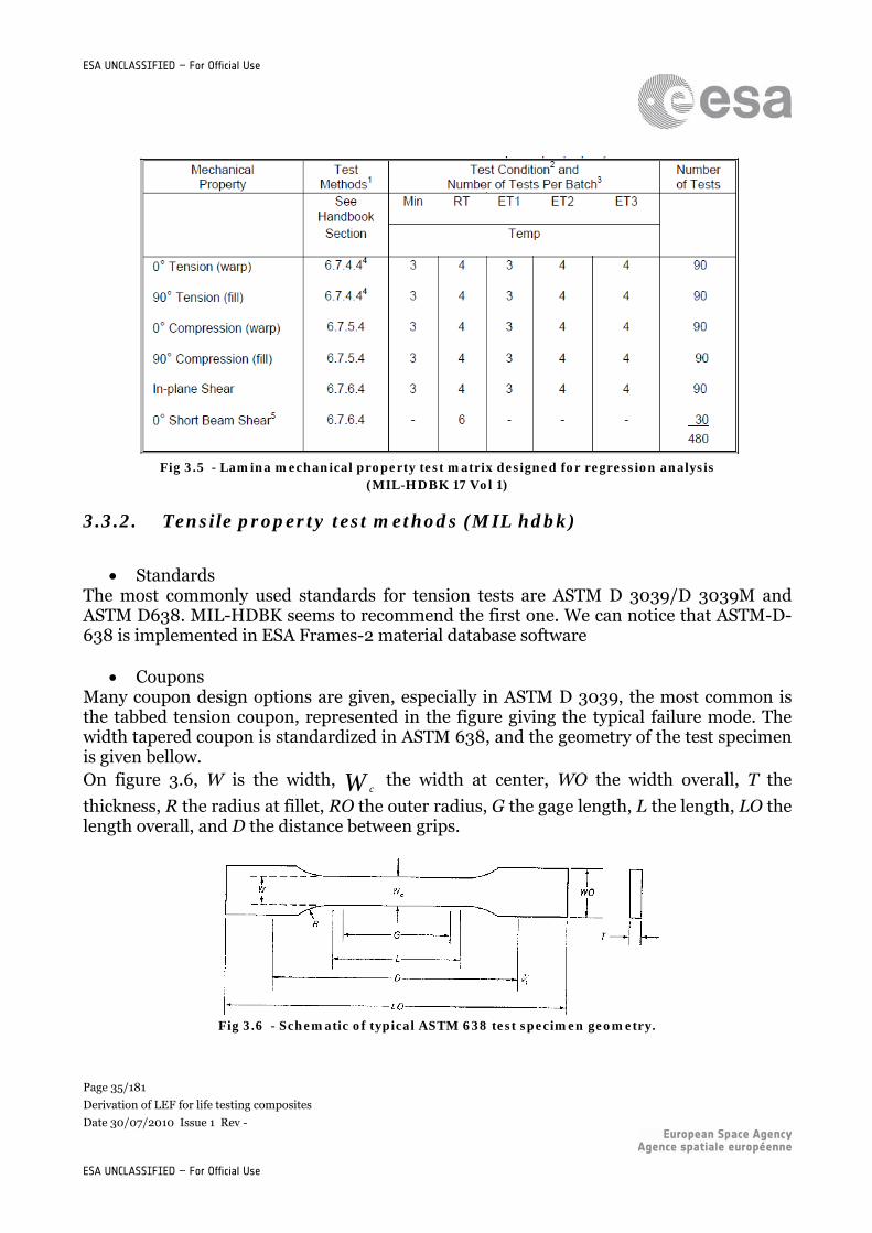
The most commonly used standards for tension tests are ASTM D 3039/D 3039M and ASTM D638. MIL-HDBK seems to recommend the first one. We can notice that ASTM-D-638 is implemented in ESA Frames-2 material database software

Coupons Many coupon design options are given, especially in ASTM D 3039, the most common is the tabbed tension coupon, represented in the figure giving the typical failure mode. The width tapered coupon is standardized in ASTM 638, and the geometry of the test specimen is given bellow. On figure 3.6, W is the width, W c

the width at center, WO the width overall, T the

thickness, R the radius at fillet, RO the outer radius, G the gage length, L the length, LO the length overall, and D the distance between grips.

Fig 3.6 - Schematic of typical ASTM 638 test specimen geometry.

Page 36/181





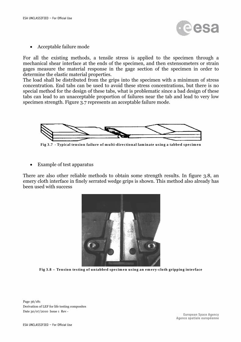
Acceptable failure mode

For all the existing methods, a tensile stress is applied to the specimen through a mechanical shear interface at the ends of the specimen, and then extensometers or strain gages measure the material response in the gage section of the specimen in order to determine the elastic material properties. The load shall be distributed from the grips into the specimen with a minimum of stress concentration. End tabs can be used to avoid these stress concentrations, but there is no special method for the design of these tabs, what is problematic since a bad design of these tabs can lead to an unacceptable proportion of failures near the tab and lead to very low specimen strength. Figure 3.7 represents an acceptable failure mode.

Fig 3.7 - Typical tension failure of multi-directional laminate using a tabbed specimen

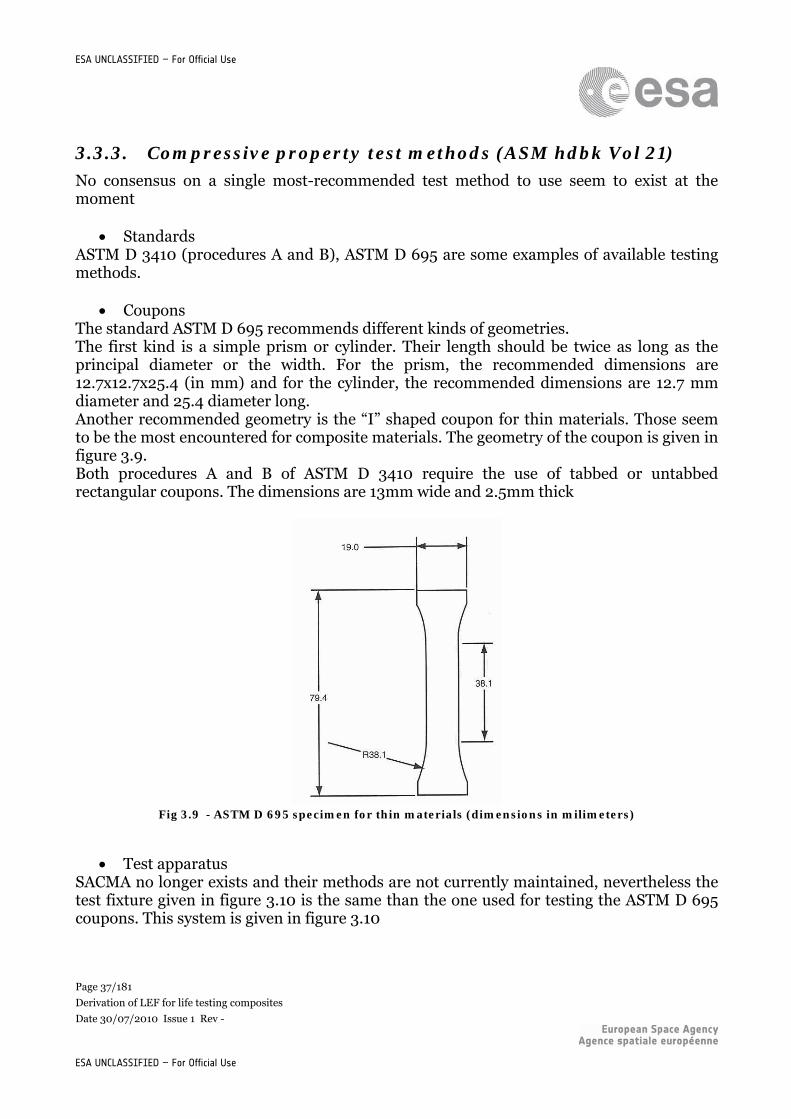
Example of test apparatus

There are also other reliable methods to obtain some strength results. In figure 3.8, an emery cloth interface in finely serrated wedge grips is shown. This method also already has been used with success

Fig 3.8 – Tension testing of untabbed specimen using an emery-cloth gripping interface

Page 37/181





3.3.3. Compressive property test methods (ASM hdbk Vol 21)

No consensus on a single most-recommended test method to use seem to exist at the moment

Standards ASTM D 3410 (procedures A and B), ASTM D 695 are some examples of available testing methods.

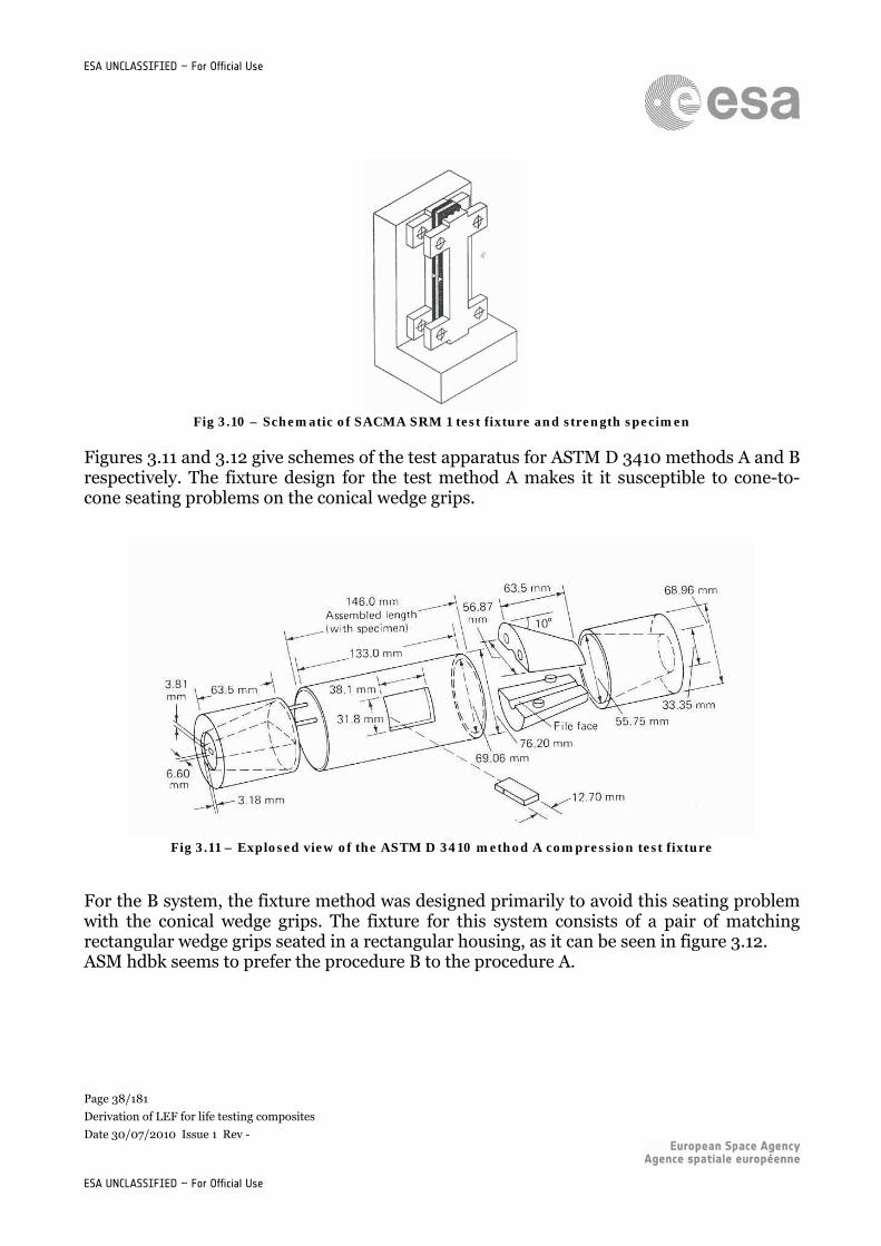
Coupons

The standard ASTM D 695 recommends different kinds of geometries. The first kind is a simple prism or cylinder. Their length should be twice as long as the principal diameter or the width. For the prism, the recommended dimensions are 12.7x12.7x25.4 (in mm) and for the cylinder, the recommended dimensions are 12.7 mm diameter and 25.4 diameter long. Another recommended geometry is the “I” shaped coupon for thin materials. Those seem to be the most encountered for composite materials. The geometry of the coupon is given in figure 3.9. Both procedures A and B of ASTM D 3410 require the use of tabbed or untabbed rectangular coupons. The dimensions are 13mm wide and 2.5mm thick

Fig 3.9 - ASTM D 695 specimen for thin materials (dimensions in milimeters)

Test apparatus SACMA no longer exists and their methods are not currently maintained, nevertheless the test fixture given in figure 3.10 is the same than the one used for testing the ASTM D 695 coupons. This system is given in figure 3.10

Page 38/181





Fig 3.10 – Schematic of SACMA SRM 1 test fixture and strength specimen

Figures 3.11 and 3.12 give schemes of the test apparatus for ASTM D 3410 methods A and B respectively. The fixture design for the test method A makes it it susceptible to cone-to-cone seating problems on the conical wedge grips.

Fig 3.11 – Explosed view of the ASTM D 3410 method A compression test fixture

For the B system, the fixture method was designed primarily to avoid this seating problem with the conical wedge grips. The fixture for this system consists of a pair of matching rectangular wedge grips seated in a rectangular housing, as it can be seen in figure 3.12. ASM hdbk seems to prefer the procedure B to the procedure A.

Page 39/181





Fig 3.12 – Schematic of compression test fixture with pyramidal wedges (ASTM D 3410 method B)

3.3.4. Shear property test methods

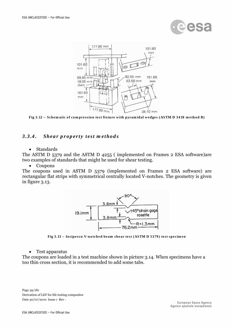
Standards The ASTM D 5379 and the ASTM D 4255 ( implemented on Frames 2 ESA software)are two examples of standards that might be used for shear testing.

Coupons The coupons used in ASTM D 5379 (implemented on Frames 2 ESA software) are rectangular flat strips with symmetrical centrally located V-notches. The geometry is given in figure 3.13.

Fig 3.13 – Iosipescu V-notched beam shear test (ASTM D 5379) test specimen

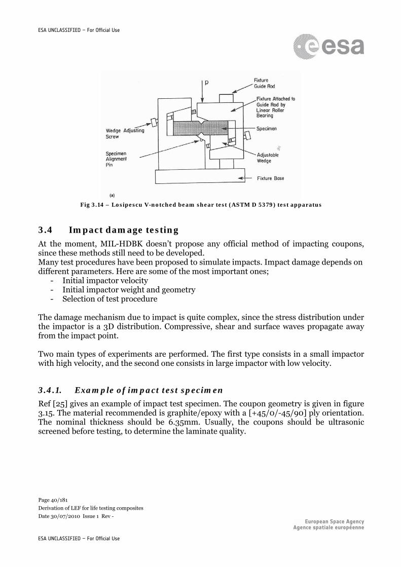
Test apparatus

The coupons are loaded in a test machine shown in picture 3.14. When specimens have a too thin cross section, it is recommended to add some tabs.

Page 40/181





Fig 3.14 – Losipescu V-notched beam shear test (ASTM D 5379) test apparatus

3.4 Impact damage testing

At the moment, MIL-HDBK doesn’t propose any official method of impacting coupons, since these methods still need to be developed. Many test procedures have been proposed to simulate impacts. Impact damage depends on different parameters. Here are some of the most important ones;

- Initial impactor velocity - Initial impactor weight and geometry - Selection of test procedure

The damage mechanism due to impact is quite complex, since the stress distribution under the impactor is a 3D distribution. Compressive, shear and surface waves propagate away from the impact point. Two main types of experiments are performed. The first type consists in a small impactor with high velocity, and the second one consists in large impactor with low velocity.

3.4.1. Example of impact test specimen

Ref [25] gives an example of impact test specimen. The coupon geometry is given in figure 3.15. The material recommended is graphite/epoxy with a [+45/0/-45/90] ply orientation. The nominal thickness should be 6.35mm. Usually, the coupons should be ultrasonic screened before testing, to determine the laminate quality.

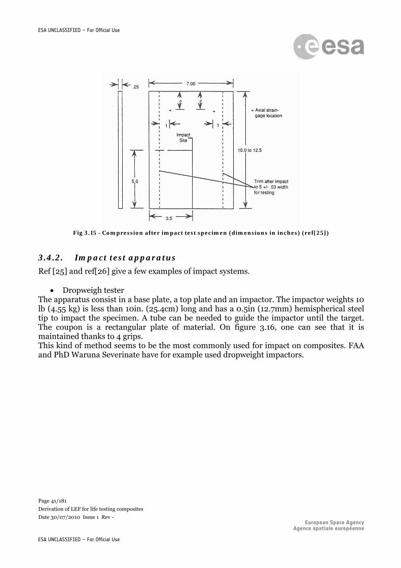
Page 41/181





Fig 3.15 - Compression after impact test specimen (dimensions in inches) (ref[25])

3.4.2. Impact test apparatus

Ref [25] and ref[26] give a few examples of impact systems.

Dropweigh tester The apparatus consist in a base plate, a top plate and an impactor. The impactor weights 10 lb (4.55 kg) is less than 10in. (25.4cm) long and has a 0.5in (12.7mm) hemispherical steel tip to impact the specimen. A tube can be needed to guide the impactor until the target. The coupon is a rectangular plate of material. On figure 3.16, one can see that it is maintained thanks to 4 grips. This kind of method seems to be the most commonly used for impact on composites. FAA and PhD Waruna Severinate have for example used dropweight impactors.

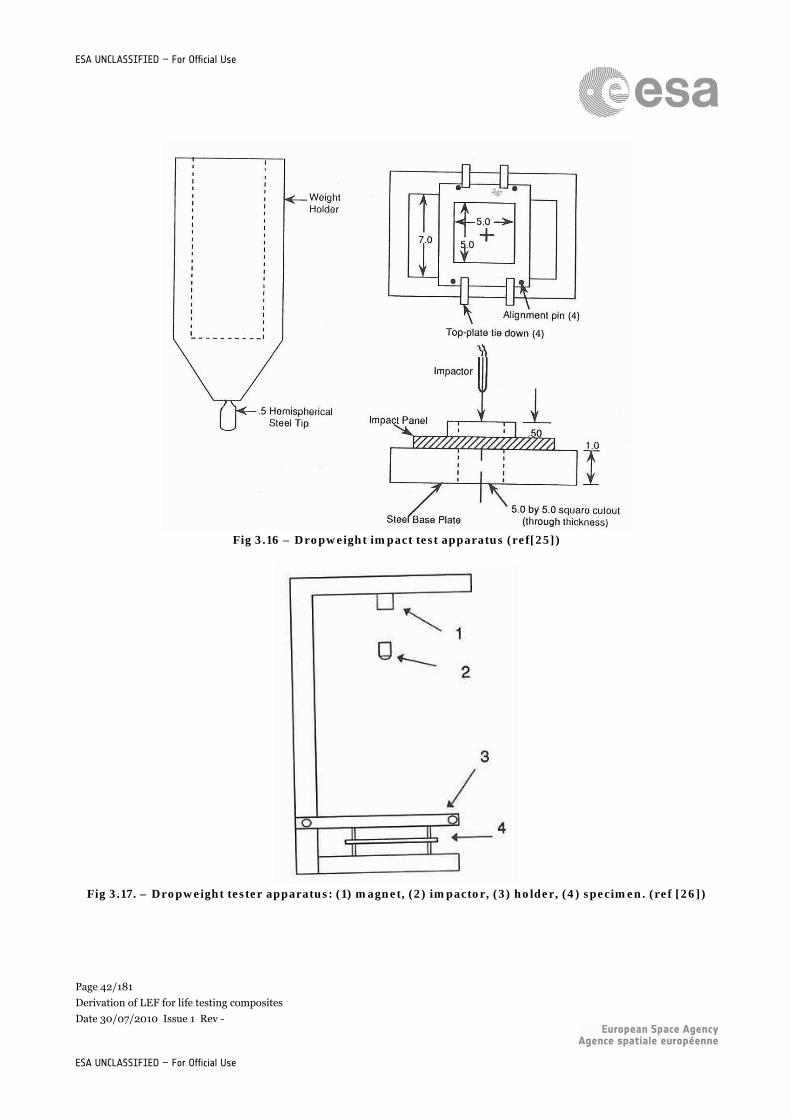
Page 42/181





Fig 3.16 – Dropweight impact test apparatus (ref[25])

Fig 3.17. – Dropweight tester apparatus: (1) magnet, (2) impactor, (3) holder, (4) specimen. (ref [26])

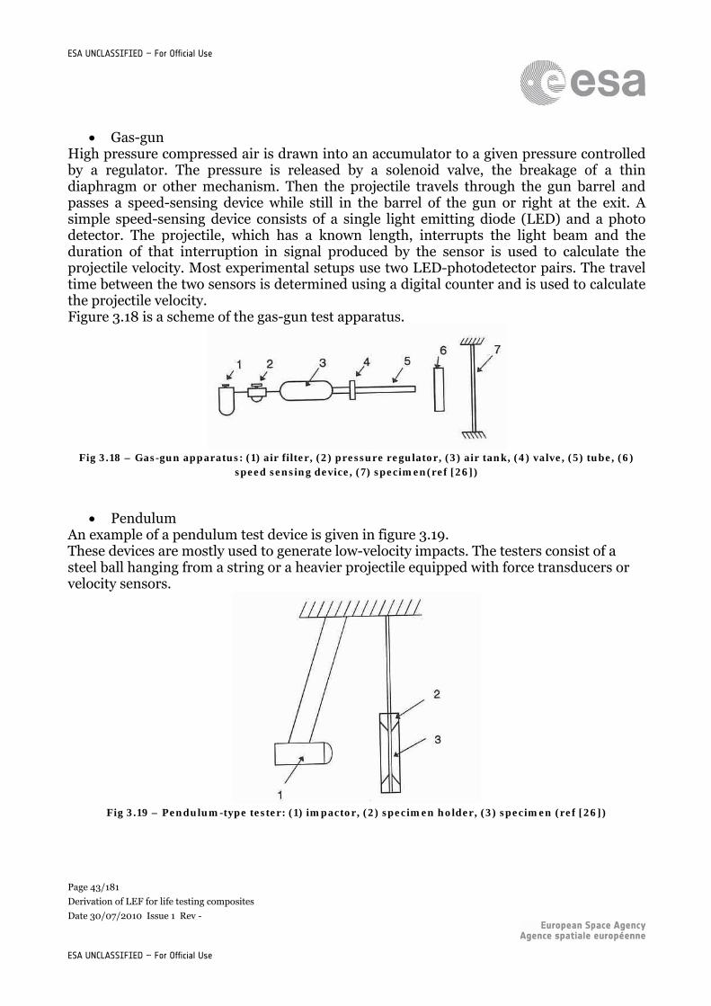
Page 43/181





Gas-gun High pressure compressed air is drawn into an accumulator to a given pressure controlled by a regulator. The pressure is released by a solenoid valve, the breakage of a thin diaphragm or other mechanism. Then the projectile travels through the gun barrel and passes a speed-sensing device while still in the barrel of the gun or right at the exit. A simple speed-sensing device consists of a single light emitting diode (LED) and a photo detector. The projectile, which has a known length, interrupts the light beam and the duration of that interruption in signal produced by the sensor is used to calculate the projectile velocity. Most experimental setups use two LED-photodetector pairs. The travel time between the two sensors is determined using a digital counter and is used to calculate the projectile velocity. Figure 3.18 is a scheme of the gas-gun test apparatus.

Fig 3.18 – Gas-gun apparatus: (1) air filter, (2) pressure regulator, (3) air tank, (4) valve, (5) tube, (6)

speed sensing device, (7) specimen(ref [26])

Pendulum An example of a pendulum test device is given in figure 3.19. These devices are mostly used to generate low-velocity impacts. The testers consist of a steel ball hanging from a string or a heavier projectile equipped with force transducers or velocity sensors.

Fig 3.19 – Pendulum-type tester: (1) impactor, (2) specimen holder, (3) specimen (ref [26])

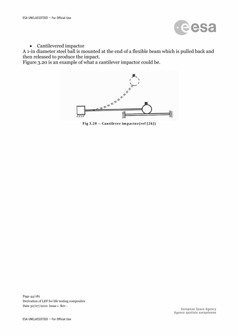
Page 44/181





Cantilevered impactor A 1-in diameter steel ball is mounted at the end of a flexible beam which is pulled back and then released to produce the impact. Figure 3.20 is an example of what a cantilever impactor could be.

Fig 3.20 – Cantilever impactor(ref [26])

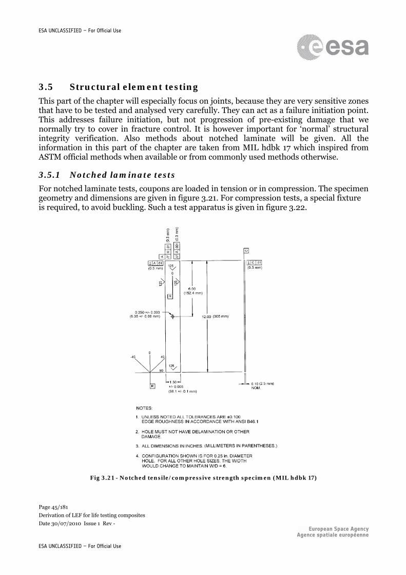
Page 45/181





3.5 Structural element testing

This part of the chapter will especially focus on joints, because they are very sensitive zones that have to be tested and analysed very carefully. They can act as a failure initiation point. This addresses failure initiation, but not progression of pre-existing damage that we normally try to cover in fracture control. It is however important for ‘normal’ structural integrity verification. Also methods about notched laminate will be given. All the information in this part of the chapter are taken from MIL hdbk 17 which inspired from ASTM official methods when available or from commonly used methods otherwise.

3.5.1 Notched laminate tests

For notched laminate tests, coupons are loaded in tension or in compression. The specimen geometry and dimensions are given in figure 3.21. For compression tests, a special fixture is required, to avoid buckling. Such a test apparatus is given in figure 3.22.

Fig 3.21 - Notched tensile/compressive strength specimen (MIL hdbk 17)

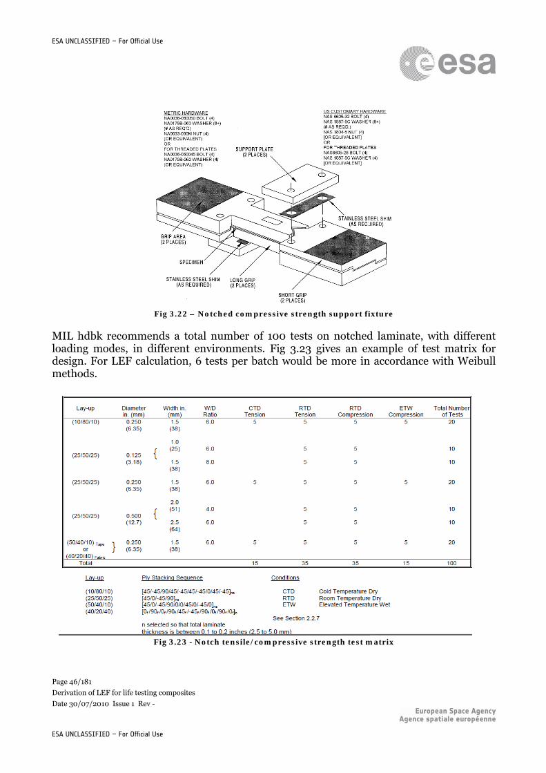
Page 46/181





Fig 3.22 – Notched compressive strength support fixture

MIL hdbk recommends a total number of 100 tests on notched laminate, with different loading modes, in different environments. Fig 3.23 gives an example of test matrix for design. For LEF calculation, 6 tests per batch would be more in accordance with Weibull methods.

Fig 3.23 - Notch tensile/compressive strength test matrix

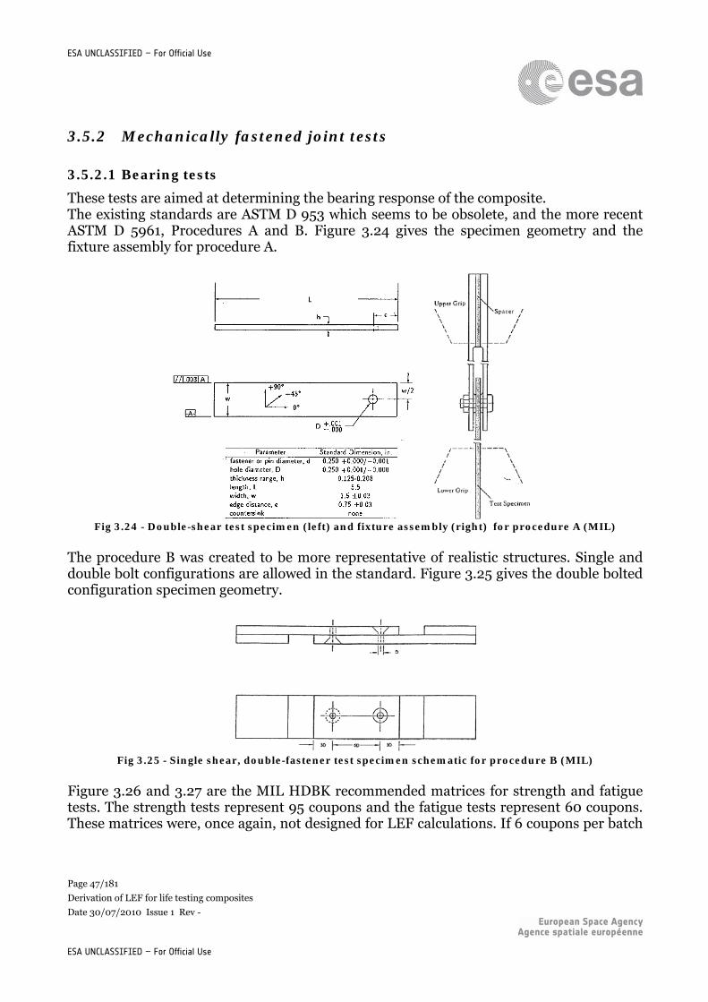
Page 47/181





3.5.2 Mechanically fastened joint tests

3.5.2.1 Bearing tests

These tests are aimed at determining the bearing response of the composite. The existing standards are ASTM D 953 which seems to be obsolete, and the more recent ASTM D 5961, Procedures A and B. Figure 3.24 gives the specimen geometry and the fixture assembly for procedure A.

Fig 3.24 - Double-shear test specimen (left) and fixture assembly (right) for procedure A (MIL)

The procedure B was created to be more representative of realistic structures. Single and double bolt configurations are allowed in the standard. Figure 3.25 gives the double bolted configuration specimen geometry.

Fig 3.25 - Single shear, double-fastener test specimen schematic for procedure B (MIL)

Figure 3.26 and 3.27 are the MIL HDBK recommended matrices for strength and fatigue tests. The strength tests represent 95 coupons and the fatigue tests represent 60 coupons. These matrices were, once again, not designed for LEF calculations. If 6 coupons per batch

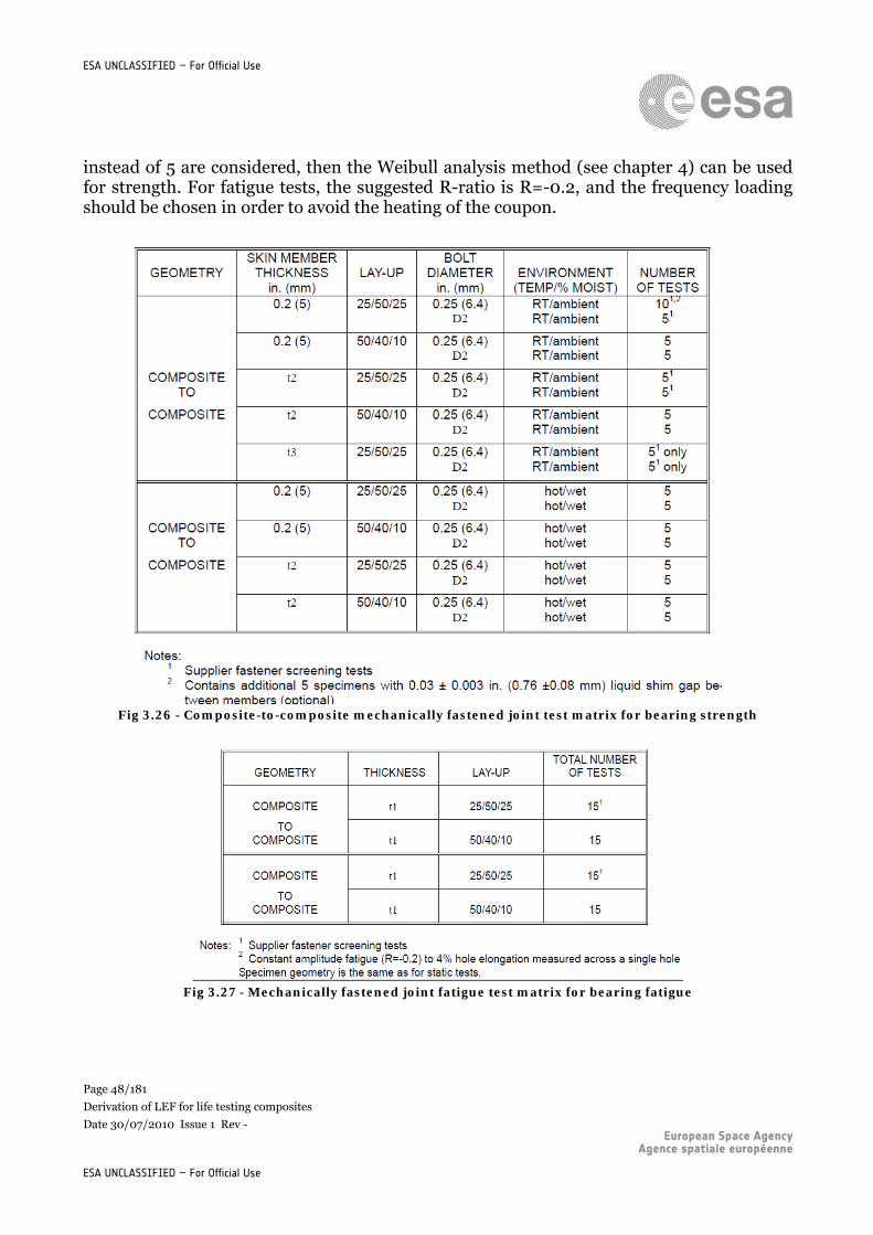
Page 48/181





instead of 5 are considered, then the Weibull analysis method (see chapter 4) can be used for strength. For fatigue tests, the suggested R-ratio is R=-0.2, and the frequency loading should be chosen in order to avoid the heating of the coupon.

Fig 3.26 - Composite-to-composite mechanically fastened joint test matrix for bearing strength

Fig 3.27 - Mechanically fastened joint fatigue test matrix for bearing fatigue

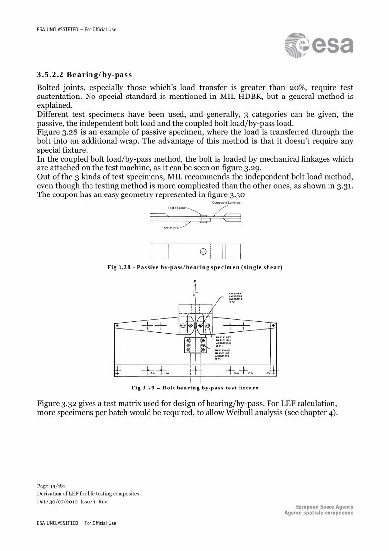
Page 49/181





3.5.2.2 Bearing/by-pass

Bolted joints, especially those which’s load transfer is greater than 20%, require test sustentation. No special standard is mentioned in MIL HDBK, but a general method is explained. Different test specimens have been used, and generally, 3 categories can be given, the passive, the independent bolt load and the coupled bolt load/by-pass load. Figure 3.28 is an example of passive specimen, where the load is transferred through the bolt into an additional wrap. The advantage of this method is that it doesn’t require any special fixture. In the coupled bolt load/by-pass method, the bolt is loaded by mechanical linkages which are attached on the test machine, as it can be seen on figure 3.29. Out of the 3 kinds of test specimens, MIL recommends the independent bolt load method, even though the testing method is more complicated than the other ones, as shown in 3.31. The coupon has an easy geometry represented in figure 3.30

Fig 3.28 - Passive by-pass/bearing specimen (single shear)

Fig 3.29 – Bolt bearing by-pass test fixture

Figure 3.32 gives a test matrix used for design of bearing/by-pass. For LEF calculation, more specimens per batch would be required, to allow Weibull analysis (see chapter 4).

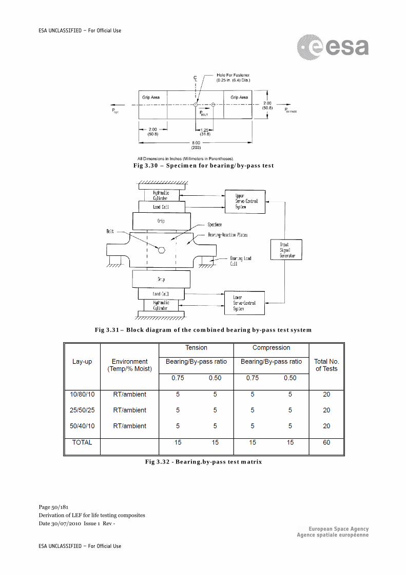
Page 50/181





Fig 3.30 – Specimen for bearing/by-pass test

Fig 3.31 – Block diagram of the combined bearing by-pass test system

Fig 3.32 - Bearing.by-pass test matrix

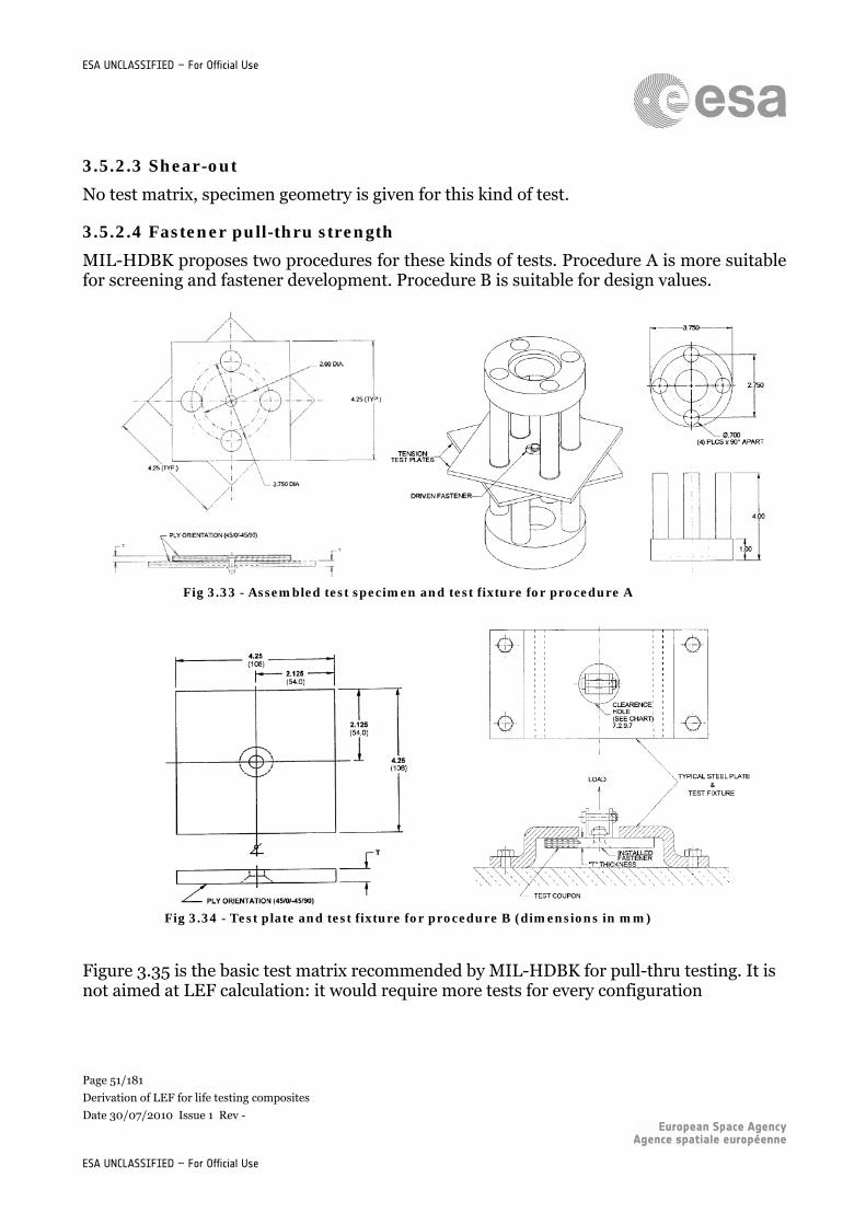
Page 51/181





3.5.2.3 Shear-out

No test matrix, specimen geometry is given for this kind of test.

3.5.2.4 Fastener pull-thru strength

MIL-HDBK proposes two procedures for these kinds of tests. Procedure A is more suitable for screening and fastener development. Procedure B is suitable for design values.

Fig 3.33 - Assembled test specimen and test fixture for procedure A

Fig 3.34 - Test plate and test fixture for procedure B (dimensions in mm)

Figure 3.35 is the basic test matrix recommended by MIL-HDBK for pull-thru testing. It is not aimed at LEF calculation: it would require more tests for every configuration

Page 52/181





Fig 3.35 - Fastener pull-thru test matrix

3.5.3 Bonded joints

3.5.3.1 Adhesive

For adhesive bonded joints, standards exist for shear and tension. For shear loading mode, the ASTM D5656 uses a thick adherent specimen as shown in figure 3.36. For this test, a special extensometer of attached to the specimen. Then the ASTM E229 uses a tubular specimen and ASTM D 1002 uses a thin single lap specimen.

Fig 3.36 – Thick adherent specimen of ASTM D 5656

Page 53/181





For tension tests, the standard describing the procedure is the ASTM D 2095. Either a rod or a bar specimen can be used. Figure 3.37 gives the geometry of the test specimen and the test fixture as described in the standard ASTM D 2095.

Fig 3.37 – Test specimen and attachment fixture

No test matrix was given, but at least 6 coupons for each test condition would be required for the statistical analysis methods.

3.5.3.2 Bonded

Many configurations of bonded joints exist. This paragraph will be a summary of the methods met in MIL-HDBK 17. For joints containing honeycomb, the standard ATSM C 297 is recommended. The test specimen and test assembly are given in figure 3.38. The dimensions in that scheme are in inches

Page 54/181





Fig 3.38 – Test specimen and attachment fixture

For skin to stiffener bond tests, the ASTM C 297 can be used. MIL HDBK recommends the “T” pull-off test specimen shown in figure 3.39 and that is quite the same than the one in ASTM C 297, except that only one block is needed here. For structures with a more flexible skin, MIL HDBK recommends is the “T” twist-off test specimen shown in picture 3.40.

Fig 3.39 – “T” pull-off specimen

Page 55/181





Fig 3.40 – “T” twist-off specimen

Double overlap joints are usually loaded in tension. Many specimen geometries exist, and their complexity depends on the structural application. The ASTM 3598-92 gives an example of test specimen geometry given in figure 3.41 that can be used for such tests. For higher load transfers, MIL HDBK would prefer the step lap joint specimen given in figure 3.42. Note that for the two test specimens, dimensions are in inches. Some other geometries are provided in MIL HDBK.

Fig 3.41 – Geometry and material of the double-lap test specimen

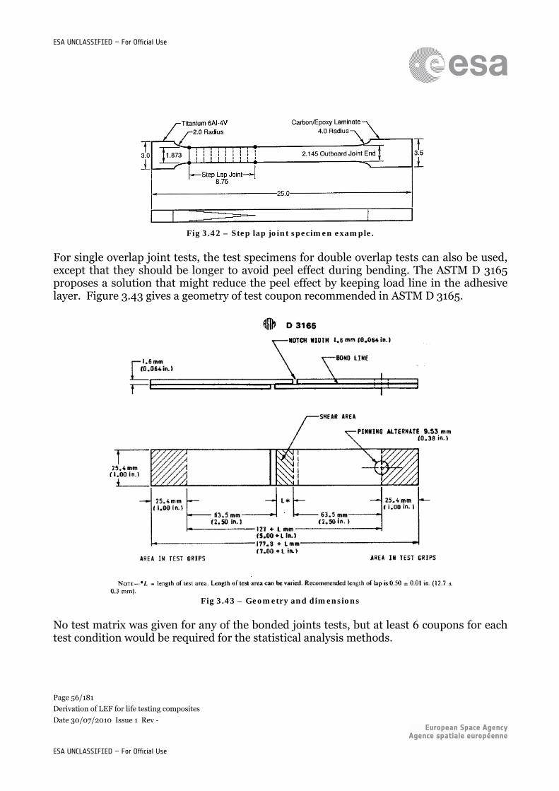
Page 56/181





Fig 3.42 – Step lap joint specimen example.

For single overlap joint tests, the test specimens for double overlap tests can also be used, except that they should be longer to avoid peel effect during bending. The ASTM D 3165 proposes a solution that might reduce the peel effect by keeping load line in the adhesive layer. Figure 3.43 gives a geometry of test coupon recommended in ASTM D 3165.

Fig 3.43 – Geometry and dimensions

No test matrix was given for any of the bonded joints tests, but at least 6 coupons for each test condition would be required for the statistical analysis methods.

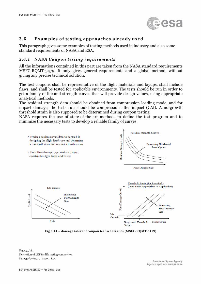
Page 57/181





3.6 Examples of testing approaches already used

This paragraph gives some examples of testing methods used in industry and also some standard requirements of NASA and ESA.

3.6.1 NASA Coupon testing requirements

All the informations contained in this part are taken from the NASA standard requirements MSFC-RQMT-3479. It only gives general requirements and a global method, without giving any precise technical solution. The test coupons shall be representative of the flight materials and layups, shall include flaws, and shall be tested for applicable environments. The tests should be run in order to get a family of life and strength curves that will provide design values, using appropriate analytical methods. The residual strength data should be obtained from compression loading mode, and for impact damage, the tests run should be compression after impact (CAI). A no-growth threshold strain is also supposed to be determined during coupon testing. NASA requires the use of state-of-the-art methods to define the test program and to minimize the necessary tests to develop a reliable family of curves.

Fig 3.44 – damage tolerant coupon test schematics (MSFC-RQMT-3479)

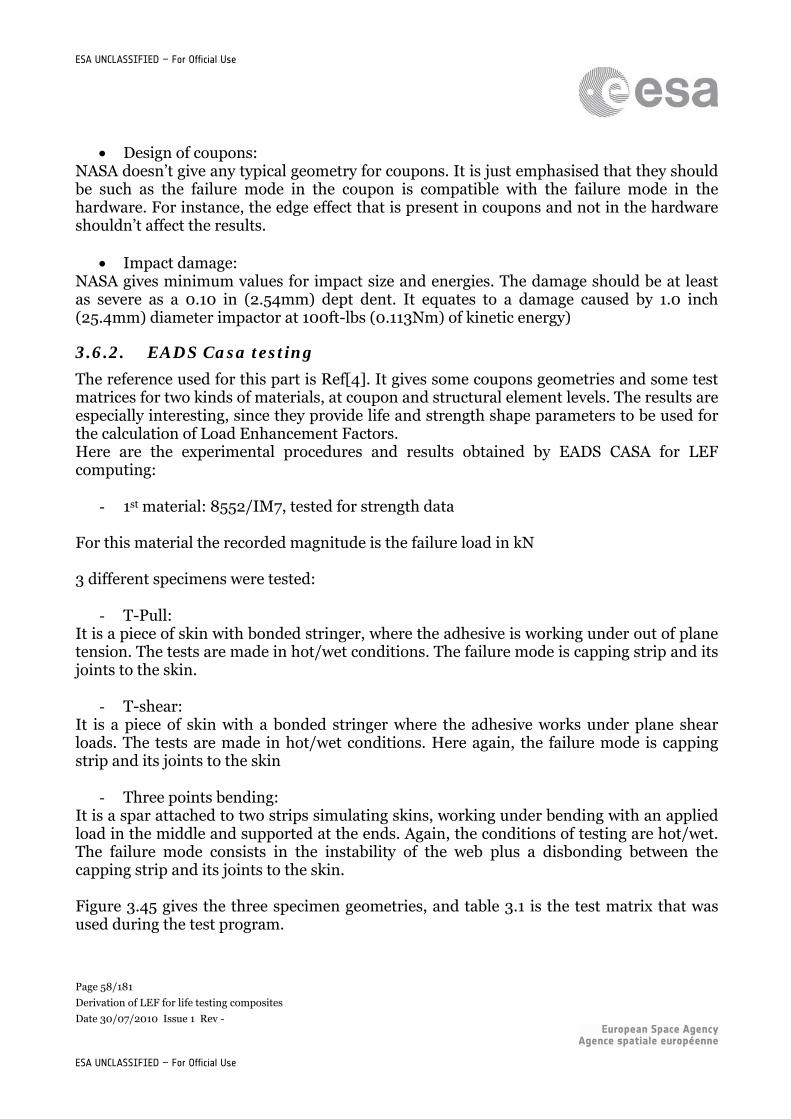
Page 58/181





Design of coupons: NASA doesn’t give any typical geometry for coupons. It is just emphasised that they should be such as the failure mode in the coupon is compatible with the failure mode in the hardware. For instance, the edge effect that is present in coupons and not in the hardware shouldn’t affect the results.

Impact damage: NASA gives minimum values for impact size and energies. The damage should be at least as severe as a 0.10 in (2.54mm) dept dent. It equates to a damage caused by 1.0 inch (25.4mm) diameter impactor at 100ft-lbs (0.113Nm) of kinetic energy)

3.6.2. EADS Casa testing

The reference used for this part is Ref[4]. It gives some coupons geometries and some test matrices for two kinds of materials, at coupon and structural element levels. The results are especially interesting, since they provide life and strength shape parameters to be used for the calculation of Load Enhancement Factors. Here are the experimental procedures and results obtained by EADS CASA for LEF computing:

- 1st material: 8552/IM7, tested for strength data For this material the recorded magnitude is the failure load in kN 3 different specimens were tested:

- T-Pull: It is a piece of skin with bonded stringer, where the adhesive is working under out of plane tension. The tests are made in hot/wet conditions. The failure mode is capping strip and its joints to the skin.

- T-shear: It is a piece of skin with a bonded stringer where the adhesive works under plane shear loads. The tests are made in hot/wet conditions. Here again, the failure mode is capping strip and its joints to the skin

- Three points bending: It is a spar attached to two strips simulating skins, working under bending with an applied load in the middle and supported at the ends. Again, the conditions of testing are hot/wet. The failure mode consists in the instability of the web plus a disbonding between the capping strip and its joints to the skin. Figure 3.45 gives the three specimen geometries, and table 3.1 is the test matrix that was used during the test program.

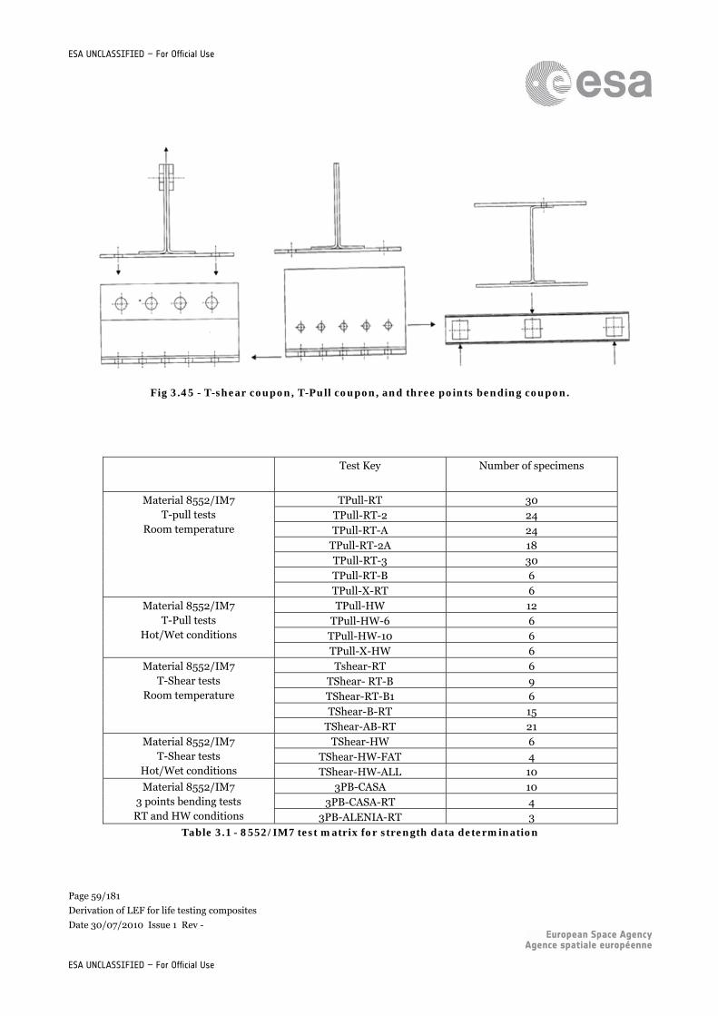
Page 59/181





Fig 3.45 - T-shear coupon, T-Pull coupon, and three points bending coupon.

Test Key Number of specimens

TPull-RT 30 TPull-RT-2 24 TPull-RT-A 24

TPull-RT-2A 18 TPull-RT-3 30 TPull-RT-B 6

Material 8552/IM7 T-pull tests

Room temperature

TPull-X-RT 6 TPull-HW 12

TPull-HW-6 6 TPull-HW-10 6

Material 8552/IM7 T-Pull tests

Hot/Wet conditions

TPull-X-HW 6 Tshear-RT 6

TShear- RT-B 9 TShear-RT-B1 6 TShear-B-RT 15

Material 8552/IM7 T-Shear tests

Room temperature

TShear-AB-RT 21 TShear-HW 6

TShear-HW-FAT 4 Material 8552/IM7

T-Shear tests Hot/Wet conditions TShear-HW-ALL 10

3PB-CASA 10 3PB-CASA-RT 4

Material 8552/IM7 3 points bending tests RT and HW conditions 3PB-ALENIA-RT 3

Table 3.1 - 8552/IM7 test matrix for strength data determination

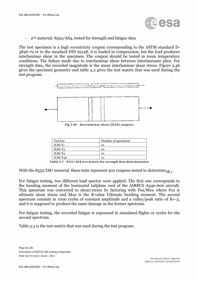
Page 60/181





- 2nd material: 8552/AS4, tested for strength and fatigue data The test specimen is a high eccentricity coupon corresponding to the ASTM standard D-3846-79 or to the standard DIN 65148, it is loaded in compression, but the load produces interlaminar shear in the specimen. The coupon should be tested in room temperature conditions. The failure mode due to interlaminar shear between interlaminate plies. For strength data, the recorded magnitude is the mean interlaminar shear stress. Figure 3.46 gives the specimen geometry and table 3.2 gives the test matrix that was used during the test program.

Fig 3.46 - Interlaminar shear (ILSS) coupons

Test key Number of specimens ILSS-T1 10 ILSS-T3 10 ILSS-T4 10 ILSS-T4A 10

Table 3.2 - 8552/AS4 test matrix for strength data determination

With the 8552/IM7 material, these tests represent 302 coupons tested to determine R.

For fatigue testing, two different load spectra were applied. The first one corresponds to the bending moment of the horizontal tailplane root of the AIRBUS A340-600 aircraft. This spectrum was converted to shear/stress by factoring with Fsu/Mxu where Fsu is ultimate shear stress and Mxu is the B-value Ultimate bending moment. The second spectrum consists in 1000 cycles of constant amplitude and a valley/peak ratio of R=-3, and it is supposed to produce the same damage as the former spectrum. For fatigue testing, the recorded fatigue is expressed in simulated flights or cycles for the second spectrum.

Table 3.3 is the test matrix that was used during the test program.

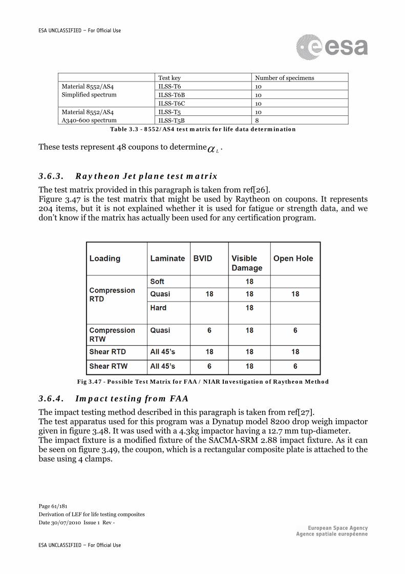
Page 61/181





Test key Number of specimens ILSS-T6 10 ILSS-T6B 10

Material 8552/AS4 Simplified spectrum

ILSS-T6C 10 ILSS-T5 10 Material 8552/AS4

A340-600 spectrum ILSS-T5B 8 Table 3.3 - 8552/AS4 test matrix for life data determination

These tests represent 48 coupons to determine L.

3.6.3. Raytheon Jet plane test matrix

The test matrix provided in this paragraph is taken from ref[26]. Figure 3.47 is the test matrix that might be used by Raytheon on coupons. It represents 204 items, but it is not explained whether it is used for fatigue or strength data, and we don’t know if the matrix has actually been used for any certification program.

Fig 3.47 - Possible Test Matrix for FAA / NIAR Investigation of Raytheon Method

3.6.4. Impact testing from FAA

The impact testing method described in this paragraph is taken from ref[27]. The test apparatus used for this program was a Dynatup model 8200 drop weigh impactor given in figure 3.48. It was used with a 4.3kg impactor having a 12.7 mm tup-diameter. The impact fixture is a modified fixture of the SACMA-SRM 2.88 impact fixture. As it can be seen on figure 3.49, the coupon, which is a rectangular composite plate is attached to the base using 4 clamps.

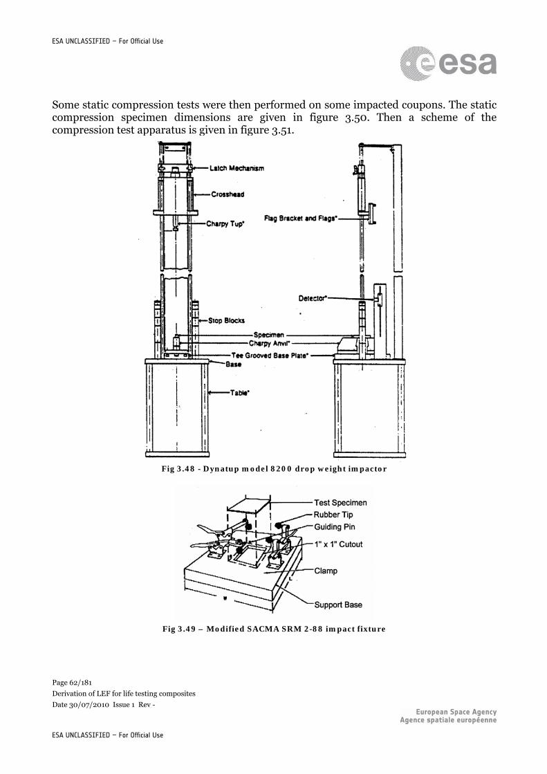
Page 62/181





Some static compression tests were then performed on some impacted coupons. The static compression specimen dimensions are given in figure 3.50. Then a scheme of the compression test apparatus is given in figure 3.51.

Fig 3.48 - Dynatup model 8200 drop weight impactor

Fig 3.49 – Modified SACMA SRM 2-88 impact fixture

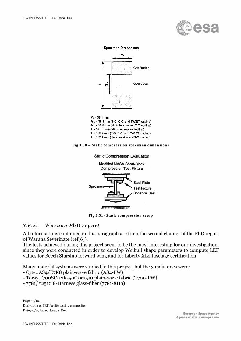
Page 63/181





Fig 3.50 – Static compression specimen dimensions

Fig 3.51 - Static compression setup

3.6.5. Waruna PhD report

All informations contained in this paragraph are from the second chapter of the PhD report of Waruna Severinate (ref[6]). The tests achieved during this project seem to be the most interesting for our investigation, since they were conducted in order to develop Weibull shape parameters to compute LEF values for Beech Starship forward wing and for Liberty XL2 fuselage certification. Many material systems were studied in this project, but the 3 main ones were: - Cytec AS4/E7K8 plain-wave fabric (AS4-PW) - Toray T700SC-12K-50C/#2510 plain-wave fabric (T700-PW) - 7781/#2510 8-Harness glass-fiber (7781-8HS)

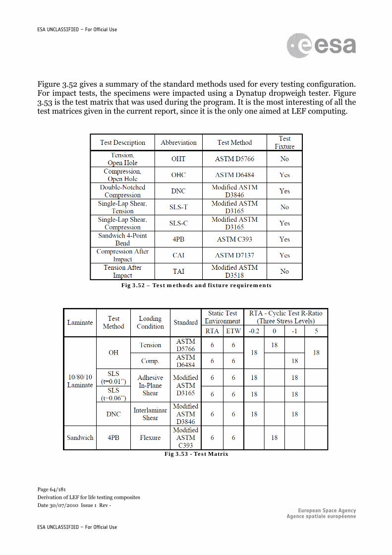
Page 64/181





Figure 3.52 gives a summary of the standard methods used for every testing configuration. For impact tests, the specimens were impacted using a Dynatup dropweigh tester. Figure 3.53 is the test matrix that was used during the program. It is the most interesting of all the test matrices given in the current report, since it is the only one aimed at LEF computing.

Fig 3.52 – Test methods and fixture requirements

Fig 3.53 - Test Matrix

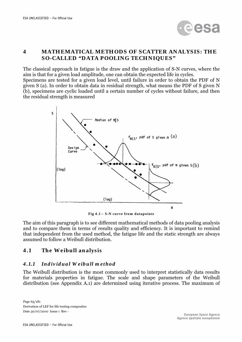
Page 65/181





4 MATHEMATICAL METHODS OF SCATTER ANALYSIS: THE SO-CALLED “DATA POOLING TECHNIQUES”

The classical approach in fatigue is the draw and the application of S-N curves, where the aim is that for a given load amplitude, one can obtain the expected life in cycles. Specimens are tested for a given load level, until failure in order to obtain the PDF of N given S (a). In order to obtain data in residual strength, what means the PDF of S given N (b), specimens are cyclic loaded until a certain number of cycles without failure, and then the residual strength is measured

Fig 4.1 – S-N curve from datapoints

The aim of this paragraph is to see different mathematical methods of data pooling analysis and to compare them in terms of results quality and efficiency. It is important to remind that independent from the used method, the fatigue life and the static strength are always assumed to follow a Weibull distribution.

4.1 The Weibull analysis

4.1.1 Individual Weibull method

The Weibull distribution is the most commonly used to interpret statistically data results for materials properties in fatigue. The scale and shape parameters of the Weibull distribution (see Appendix A.1) are determined using iterative process. The maximum of

(a)

(b)

Page 66/181





likelihood estimation can be used (see Appendix A.2.), but it requires samples containing more than 20 or 30 points. The rank regression in X method is then used to determine α and β. For fatigue data, each stress level is analyzed, and then the shape parameters are arithmetically averaged to define life scatter. Weibull analysis considers only the data at a certain stress level at a time, this is the reason why six or more data points must be included in each stress level with at least five distinct stress levels. This represents at the end a very large amount of data points.

4.1.2 Joint Weibull method

In this analysis, M groups of data having a common shape parameter but different scale parameter are pooled. This means, for example for fatigue data, beta will be different since the average lifetime will be different for every stress level, but the alpha will be the same, since it is supposed to be the same for one material. Indeed, an important assumption needs to be done before the analysis: the individual shape parameter value is independent of the fatigue stress level. The output of this analysis are the shape and scale parameters of the Weibull distribution. The shape and scale parameters of the Joint Weibull analysis are obtained by the joint maximum likelihood estimate method. This analysis is similar to that described in Appendix 1.3. for a basic 2-parameter Weibull distribution. However, the joint maximum likelihood estimate is applied to M groups of data by assuming their shape parameters are not significantly different. The shape and scale parameters can be found solving the following equations:

0

)ln(

ˆ

)ln(

1

1

1

1

ˆ

1

ˆ

M

i fi

jijM

i

jij

jijij

n

x

x

xxn

Mn

n fi

i

i

(4.a)

ni

jij

fix

ni 1

ˆ1ˆˆ

1

(4.b)

with:

ni the number of data points in the ith

group

nfi the number of failures points in the ith

group

Page 67/181





4.2 The Sendeckyj analysis

The Sendeckyj method proposes to analyse and interpret fatigue data in experiments in order to characterize the S-N behaviour of composites materials. This method is much more complex than the two Weibull analysis methods and will therefore be described more in details. The outputs of the Sendeckyj analysis procedure are:

Parameters of the deterministic equation (fatigue model parameters) Weibull parameters of the life distribution

Three main assumptions need to be done before starting the procedure:

S-N behaviour is described by a deterministic equation, based on either theoretical considerations or experimental observations of the fatigue damage accumulation process.

The static strength is uniquely related to the fatigue lives and residual strengths at runout. The relationship assumed is that the strongest specimen has either the longest fatigue life or the highest residual strength at runout. But this assumption is not fulfilled if different failure modes are observed during the fatigue test, which means that the range of validity might be limited.

The static strength data can be described by a 2-parameter Weibull distribution. This kind of distribution has been chosen because it provides a good fit of the static strength data for composites materials.

This method can be applied to any fatigue model, but for the present case, the wearout model will be used as an example of application of the method, as proposed by Sendeckyj.

4.2.1 Nature of Fatigue Data

- Static strength data:

Tensile or compressive static strength S at a

loading rate, encountered during fatigue

testing.

- Fatigue failure data: Number of cycles N to failure at an applied cyclic stress a

.

- Residual strength data:

Residual strength R after a number of cycles n at some applied cyclic stress a

. The

residual strength data for a strain-rate sensitive material must be at loading rate corresponding to the cyclic loading rate.

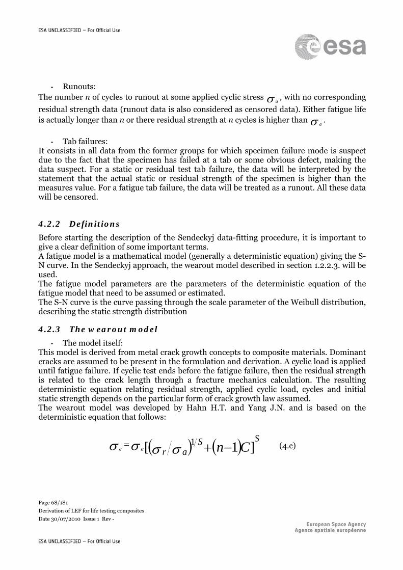
Page 68/181





- Runouts:

The number n of cycles to runout at some applied cyclic stress a, with no corresponding

residual strength data (runout data is also considered as censored data). Either fatigue life is actually longer than n or there residual strength at n cycles is higher than a

.

- Tab failures:

It consists in all data from the former groups for which specimen failure mode is suspect due to the fact that the specimen has failed at a tab or some obvious defect, making the data suspect. For a static or residual test tab failure, the data will be interpreted by the statement that the actual static or residual strength of the specimen is higher than the measures value. For a fatigue tab failure, the data will be treated as a runout. All these data will be censored.

4.2.2 Definitions

Before starting the description of the Sendeckyj data-fitting procedure, it is important to give a clear definition of some important terms. A fatigue model is a mathematical model (generally a deterministic equation) giving the S-N curve. In the Sendeckyj approach, the wearout model described in section 1.2.2.3. will be used. The fatigue model parameters are the parameters of the deterministic equation of the fatigue model that need to be assumed or estimated. The S-N curve is the curve passing through the scale parameter of the Weibull distribution, describing the static strength distribution

4.2.3 The wearout model

- The model itself: This model is derived from metal crack growth concepts to composite materials. Dominant cracks are assumed to be present in the formulation and derivation. A cyclic load is applied until fatigue failure. If cyclic test ends before the fatigue failure, then the residual strength is related to the crack length through a fracture mechanics calculation. The resulting deterministic equation relating residual strength, applied cyclic load, cycles and initial static strength depends on the particular form of crack growth law assumed. The wearout model was developed by Hahn H.T. and Yang J.N. and is based on the deterministic equation that follows:

]1[ 1 CnarS S

ae (4.c)

Page 69/181





With:

e the equivalent static strength

a the maximum applied cyclic stress

r the residual strength

n the number of cycles S the absolute value of the asymptotic slope at long life on a log-log plot of the S-N curve C a measure of the extent of the flat region on the S-N curve at high applied cyclic stress levels.

Then, the wearout model assumes that the equivalent static strength follows a 2-parameters Weibull distribution (see appendix A) Thanks to the definition of the Weibull distribution, one can say that the probability that the static strength exceeds e

is given by:

]exp[)( )(

ePe

(4.c)

- Manipulation of the wearout model equation:

In case of fatigue failure, a

= r and n = N. The wearout model equation becomes then

]1[ NCC Sae (4.d)

Gives the fatigue failure criterion that gives the shape of the S-N curve If C=1, former eq reduces to power low fatigue failure criterion If C>1, this behaviour has never been observed on composites If C<1, this behaviour is often observed on composites This effect of C in the aspect of the S-N curve can be seen on figure 4.2.

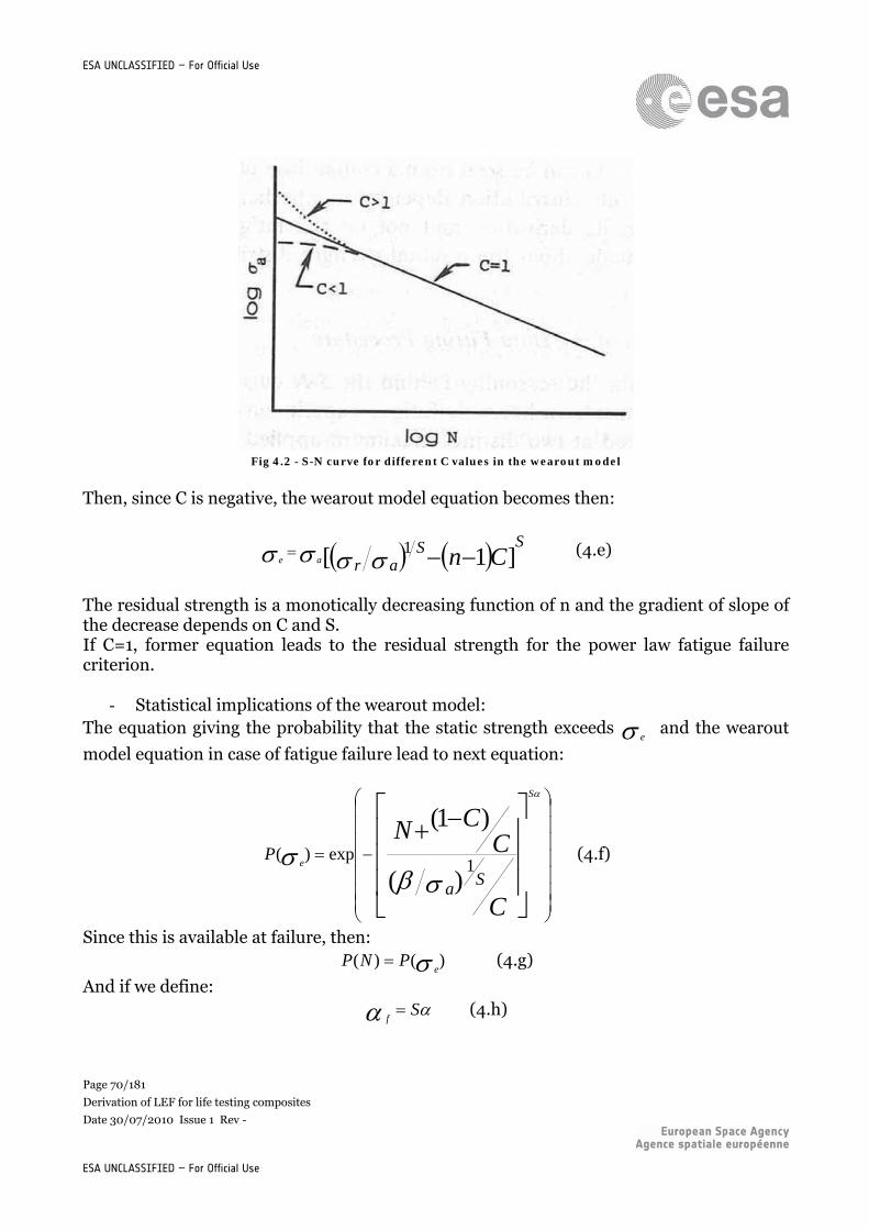
Page 70/181





Fig 4.2 - S-N curve for different C values in the wearout model

Then, since C is negative, the wearout model equation becomes then:

]1[ 1 CnarS S

ae (4.e)

The residual strength is a monotically decreasing function of n and the gradient of slope of the decrease depends on C and S. If C=1, former equation leads to the residual strength for the power law fatigue failure criterion.

- Statistical implications of the wearout model: The equation giving the probability that the static strength exceeds e

and the wearout

model equation in case of fatigue failure lead to next equation:

C

CCN

a S

P

S

e

)(

)1(

1exp)(

(4.f)

Since this is available at failure, then: )()( e

PNP (4.g)

And if we define: S

f (4.h)

Page 71/181





Ca

S

f

)(1

(4.i)

CCA )1( (4.j)

Then former equation (4.g) becomes

f

NPAN

f

exp)( (4.k)

This equation is the definition of a 3-parameters Weibull distribution with f,

f and A

as respectively shape, scale and location parameters. In former equation, the case A<0 cannot occur, because it is physically impossible to have negative lives. To solve this problem, one use conditional probabilities in deriving the expression for fatigue life from the reliability function for the static strength distribution. The reliability such that ae

is given by:

aePaee

exp)( (4.l)

The equation of the 3-parameters Weibull distribution becomes then:

a

fNP AN

f

aeexp)( (4.m)

This equation is not a Weibull distribution anymore. The form of the fatigue life distribution depends on whether conditional probabilities are used in its derivation and not on the fatigue model. If the same kind of assumptions are made on static strength, then the method could also be used for static strength.

4.2.4 Method to obtain fatigue model parameters of the wearout model

For an available set of fatigue data:

1=highest maximum applied cyclic stress value

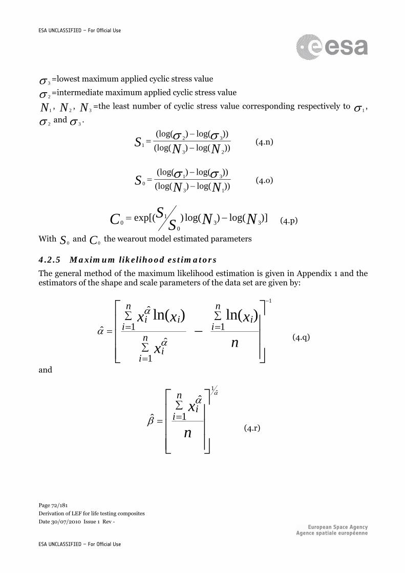
Page 72/181





3=lowest maximum applied cyclic stress value

2=intermediate maximum applied cyclic stress value

N1, N 2

, N 3=the least number of cyclic stress value corresponding respectively to 1

,

2 and 3

.

))log()(log(

))log()(log(

23

321 NNS

(4.n)

))log()(log(

))log()(log(

13

310 NNS

(4.o)

)]log()log()exp[(33

0

10 NNS

SC (4.p)

With S 0 and C0

the wearout model estimated parameters

4.2.5 Maximum likelihood estimators

The general method of the maximum likelihood estimation is given in Appendix 1 and the estimators of the shape and scale parameters of the data set are given by:

n

x

x

xxn

ii

n

ii

n

iii

1

1

ˆ

1

ˆ

ˆ

)ln()ln(1

(4.q)

and

n

xn

ii

1

ˆ

ˆ

ˆ1

(4.r)

Page 73/181





4.2.6 The Sendeckyj data-fitting procedure

The procedure is divided in seven steps as follows: 1. Create a traceability system in order to be able to know which e

value comes from

which data. Such a system is required to censor unusable values for the following steps (maximum likelihood, goodness-of-fit)

2. Choose a fatigue model to fit the fatigue data. In this approach, the wearout model

previously described will be used. Its parameters are C and S. 3. Assume or estimate the model parameters values. In the current study, the S 0

and

C0 values obtained in section 1.2.2.4 will be the chosen estimates.

4. Compute e

, S 0 and C0

values from the fatigue data using the fatigue model. e

should follow a Weibull distribution. 5. Thanks to the method explained in section 1.2.2.5. compute the maximum of

likelihood estimators of the shape and scale parameter of the Weibull distribution of

e.

6. Select a new set of C and S values and repeat the method until the maximum shape parameter α is found. This maximum α value and its corresponding β, S and C value constitute the best fit of the fatigue data.

7. The last step consists in plotting the probability of survival as a function of e

. This

curve will be obtained by plotting e values corresponding to the static strength

and fatigue data at the different a levels. If the two sets of data intersperse, the

fatigue model can be considered to fit the fatigue data. A last fitting check can be done thanks to the goodness-to-fit test or thanks to the Kruskal-Wallis test. Figure 3.2 is an example of such a plot.

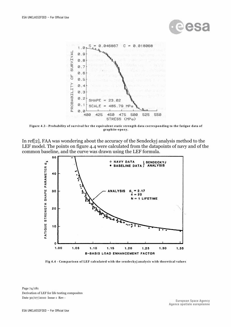
Page 74/181





Figure 4.3 - Probability of survival for the equivalent static strength data corresponding to the fatigue data of

graphite-epoxy.

In ref[2], FAA was wondering about the accuracy of the Sendeckyj analysis method to the LEF model. The points on figure 4.4 were calculated from the datapoints of navy and of the common baseline, and the curve was drawn using the LEF formula.

Fig 4.4 - Comparison of LEF calculated with the sendeckyj analysis with thoretical values

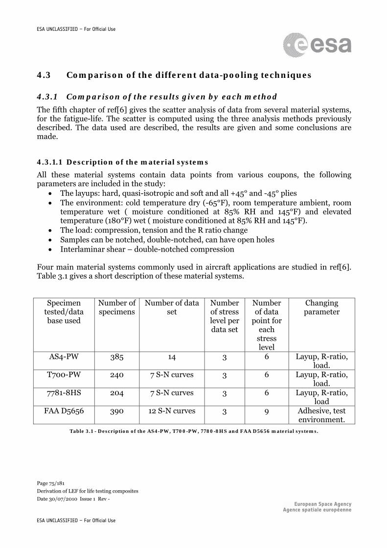
Page 75/181





4.3 Comparison of the different data-pooling techniques

4.3.1 Comparison of the results given by each method

The fifth chapter of ref[6] gives the scatter analysis of data from several material systems, for the fatigue-life. The scatter is computed using the three analysis methods previously described. The data used are described, the results are given and some conclusions are made.

4.3.1.1 Description of the material systems

All these material systems contain data points from various coupons, the following parameters are included in the study:

The layups: hard, quasi-isotropic and soft and all +45° and -45° plies The environment: cold temperature dry (-65°F), room temperature ambient, room

temperature wet ( moisture conditioned at 85% RH and 145°F) and elevated temperature (180°F) wet ( moisture conditioned at 85% RH and 145°F).

The load: compression, tension and the R ratio change Samples can be notched, double-notched, can have open holes Interlaminar shear – double-notched compression

Four main material systems commonly used in aircraft applications are studied in ref[6]. Table 3.1 gives a short description of these material systems.

Specimen tested/data base used

Number of specimens

Number of data set

Number of stress level per data set

Number of data

point for each

stress level

Changing parameter

AS4-PW 385 14 3 6 Layup, R-ratio, load.

T700-PW 240 7 S-N curves 3 6 Layup, R-ratio, load.

7781-8HS 204 7 S-N curves 3 6 Layup, R-ratio, load

FAA D5656 390 12 S-N curves 3 9 Adhesive, test environment.

Table 3.1 - Description of the AS4-PW, T700-PW, 7780-8HS and FAA D5656 material systems.

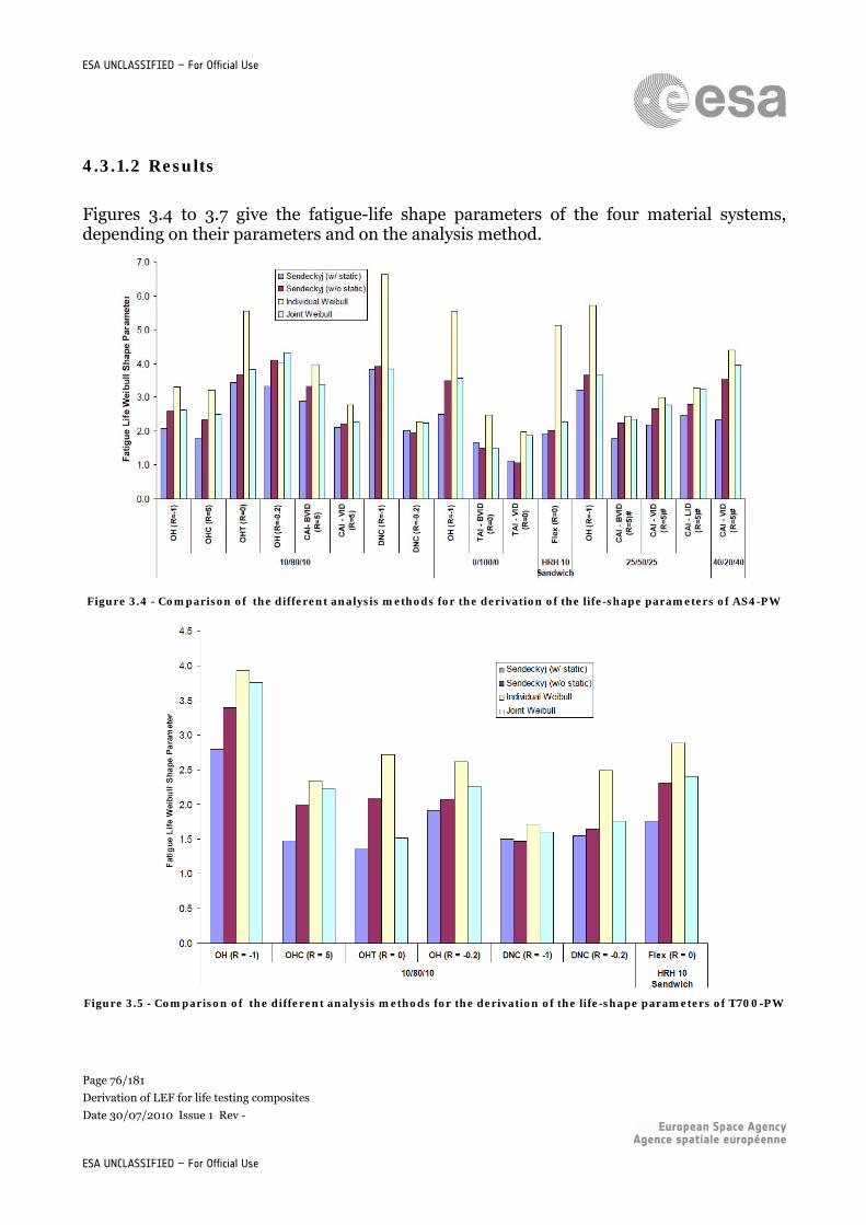
Page 76/181





4.3.1.2 Results

Figures 3.4 to 3.7 give the fatigue-life shape parameters of the four material systems, depending on their parameters and on the analysis method.

Figure 3.4 - Comparison of the different analysis methods for the derivation of the life-shape parameters of AS4-PW

Figure 3.5 - Comparison of the different analysis methods for the derivation of the life-shape parameters of T700-PW

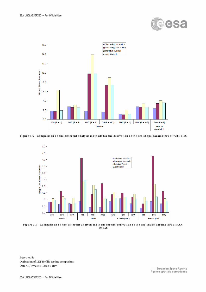
Page 77/181





Figure 3.6 - Comparison of the different analysis methods for the derivation of the life-shape parameters of 7781-8HS

Figure 3.7 - Comparison of the different analysis methods for the derivation of the life-shape parameters of FAA-

D5656

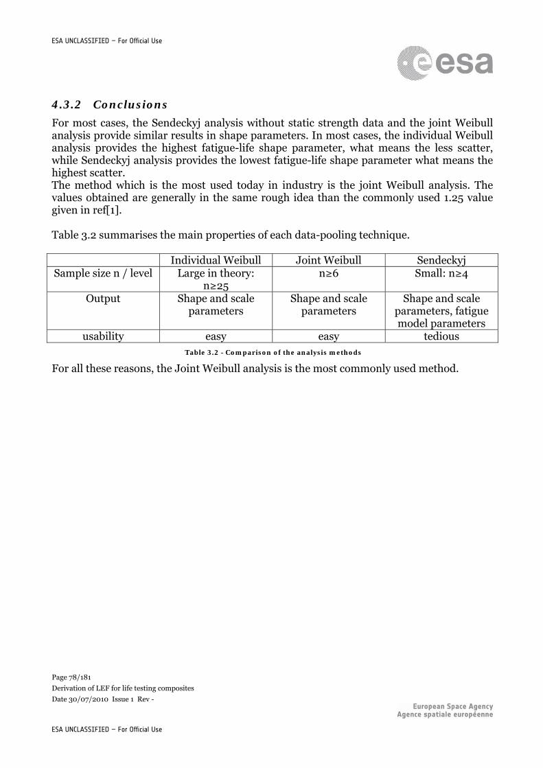
Page 78/181





4.3.2 Conclusions

For most cases, the Sendeckyj analysis without static strength data and the joint Weibull analysis provide similar results in shape parameters. In most cases, the individual Weibull analysis provides the highest fatigue-life shape parameter, what means the less scatter, while Sendeckyj analysis provides the lowest fatigue-life shape parameter what means the highest scatter. The method which is the most used today in industry is the joint Weibull analysis. The values obtained are generally in the same rough idea than the commonly used 1.25 value given in ref[1]. Table 3.2 summarises the main properties of each data-pooling technique. Individual Weibull Joint Weibull Sendeckyj Sample size n / level Large in theory:

n≥25 n≥6 Small: n≥4

Output Shape and scale parameters

Shape and scale parameters

Shape and scale parameters, fatigue model parameters

usability easy easy tedious Table 3.2 - Comparison of the analysis methods

For all these reasons, the Joint Weibull analysis is the most commonly used method.

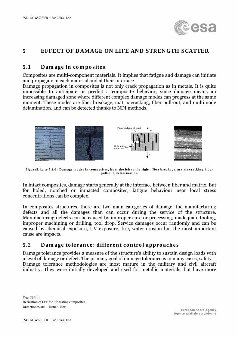
Page 79/181





5 EFFECT OF DAMAGE ON LIFE AND STRENGTH SCATTER

5.1 Damage in composites

Composites are multi-component materials. It implies that fatigue and damage can initiate and propagate in each material and at their interface. Damage propagation in composites is not only crack propagation as in metals. It is quite impossible to anticipate or predict a composite behavior, since damage means an increasing damaged zone where different complex damage modes can progress at the same moment. These modes are fiber breakage, matrix cracking, fiber pull-out, and multimode delamination, and can be detected thanks to NDI methods.

Figure5.1.a to 5.1.d : Damage modes in composites, from the left to the right: fiber breakage, matrix cracking, fiber pull-out, delamination

In intact composites, damage starts generally at the interface between fiber and matrix. But for holed, notched or impacted composites, fatigue behaviour near local stress concentrations can be complex. In composites structures, there are two main categories of damage, the manufacturing defects and all the damages than can occur during the service of the structure. Manufacturing defects can be caused by improper cure or processing, inadequate tooling, improper machining or drilling, tool drop. Service damages occur randomly and can be caused by chemical exposure, UV exposure, fire, water erosion but the most important cause are impacts.

5.2 Damage tolerance: different control approaches

Damage tolerance provides a measure of the structure’s ability to sustain design loads with a level of damage or defect. The primary goal of damage tolerance is in many cases, safety. Damage tolerance methodologies are most mature in the military and civil aircraft industry. They were initially developed and used for metallic materials, but have more

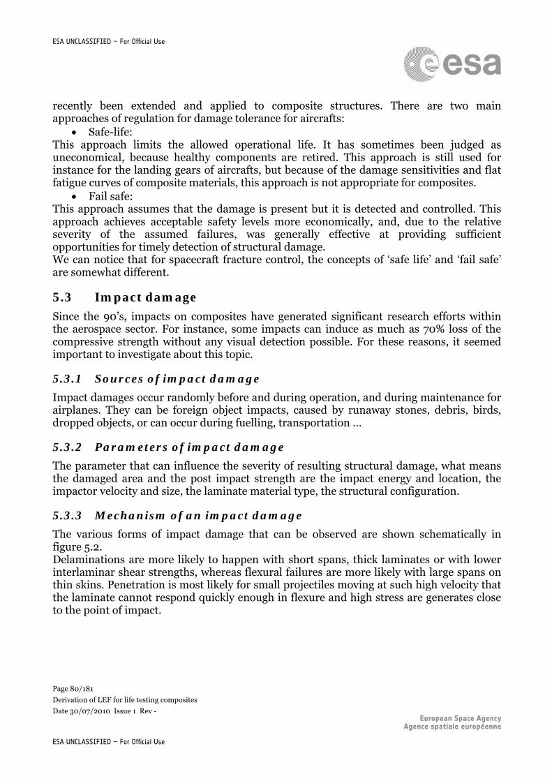
Page 80/181





recently been extended and applied to composite structures. There are two main approaches of regulation for damage tolerance for aircrafts:

Safe-life: This approach limits the allowed operational life. It has sometimes been judged as uneconomical, because healthy components are retired. This approach is still used for instance for the landing gears of aircrafts, but because of the damage sensitivities and flat fatigue curves of composite materials, this approach is not appropriate for composites.

Fail safe: This approach assumes that the damage is present but it is detected and controlled. This approach achieves acceptable safety levels more economically, and, due to the relative severity of the assumed failures, was generally effective at providing sufficient opportunities for timely detection of structural damage. We can notice that for spacecraft fracture control, the concepts of ‘safe life’ and ‘fail safe’ are somewhat different.

5.3 Impact damage

Since the 90’s, impacts on composites have generated significant research efforts within the aerospace sector. For instance, some impacts can induce as much as 70% loss of the compressive strength without any visual detection possible. For these reasons, it seemed important to investigate about this topic.

5.3.1 Sources of impact damage

Impact damages occur randomly before and during operation, and during maintenance for airplanes. They can be foreign object impacts, caused by runaway stones, debris, birds, dropped objects, or can occur during fuelling, transportation …

5.3.2 Parameters of impact damage

The parameter that can influence the severity of resulting structural damage, what means the damaged area and the post impact strength are the impact energy and location, the impactor velocity and size, the laminate material type, the structural configuration.

5.3.3 Mechanism of an impact damage

The various forms of impact damage that can be observed are shown schematically in figure 5.2. Delaminations are more likely to happen with short spans, thick laminates or with lower interlaminar shear strengths, whereas flexural failures are more likely with large spans on thin skins. Penetration is most likely for small projectiles moving at such high velocity that the laminate cannot respond quickly enough in flexure and high stress are generates close to the point of impact.

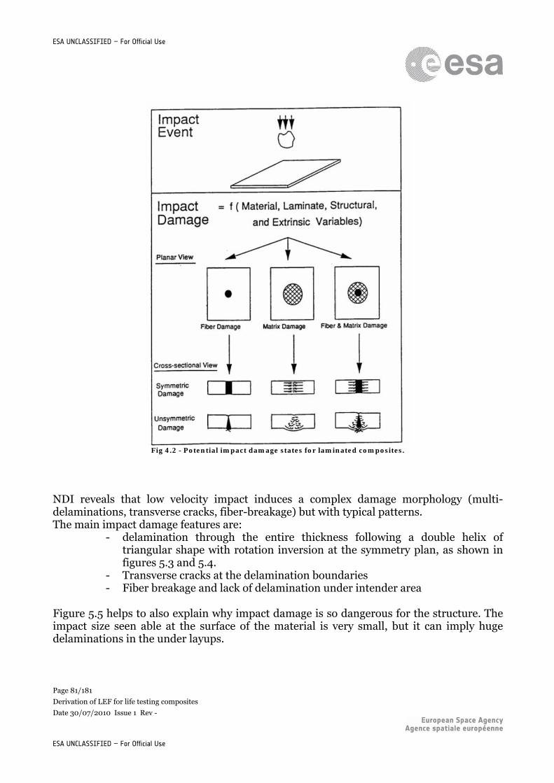
Page 81/181





Fig 4.2 - Potential impact damage states for laminated composites.

NDI reveals that low velocity impact induces a complex damage morphology (multi-delaminations, transverse cracks, fiber-breakage) but with typical patterns. The main impact damage features are:

- delamination through the entire thickness following a double helix of triangular shape with rotation inversion at the symmetry plan, as shown in figures 5.3 and 5.4.

- Transverse cracks at the delamination boundaries - Fiber breakage and lack of delamination under intender area

Figure 5.5 helps to also explain why impact damage is so dangerous for the structure. The impact size seen able at the surface of the material is very small, but it can imply huge delaminations in the under layups.

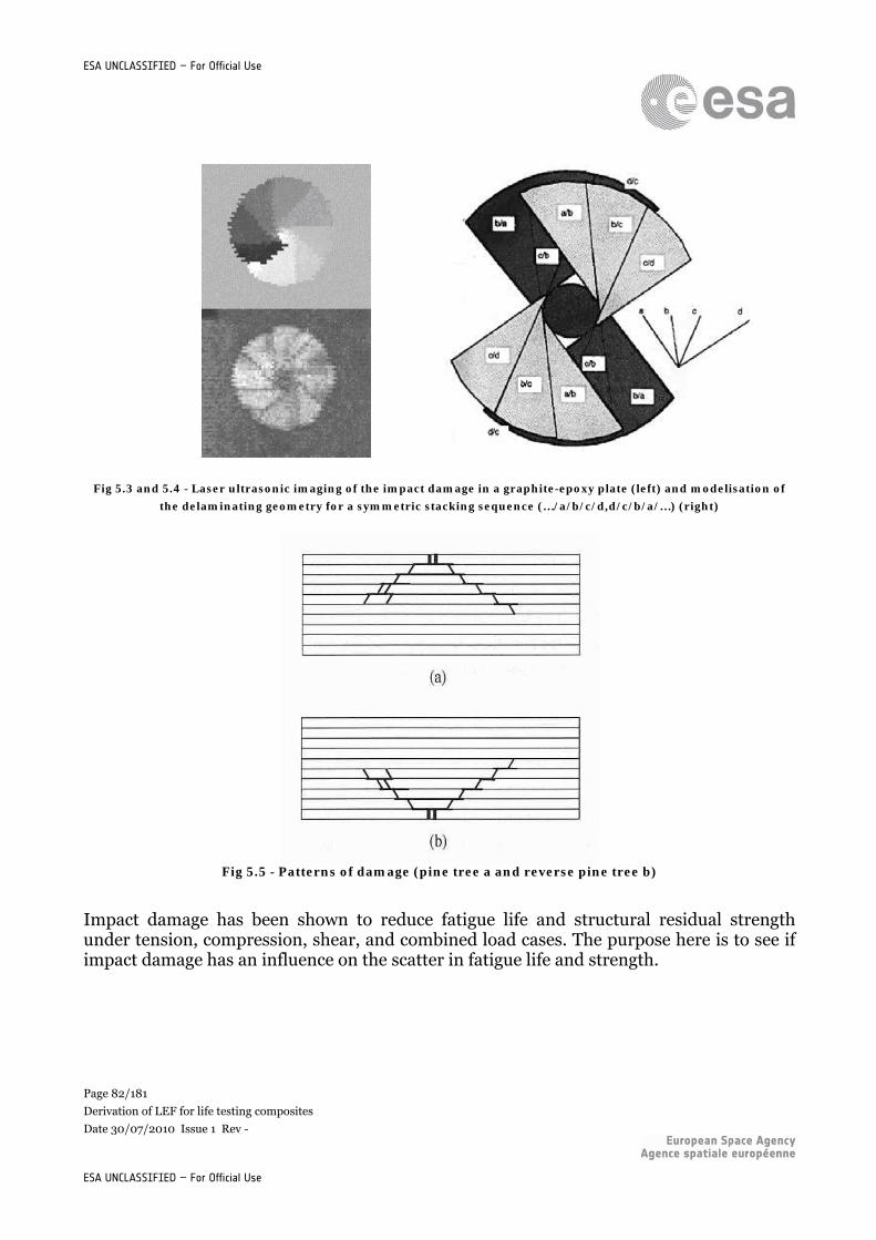
Page 82/181





Fig 5.3 and 5.4 - Laser ultrasonic imaging of the impact damage in a graphite-epoxy plate (left) and modelisation of

the delaminating geometry for a symmetric stacking sequence (…/a/b/c/d,d/c/b/a/…) (right)

Fig 5.5 - Patterns of damage (pine tree a and reverse pine tree b)

Impact damage has been shown to reduce fatigue life and structural residual strength under tension, compression, shear, and combined load cases. The purpose here is to see if impact damage has an influence on the scatter in fatigue life and strength.

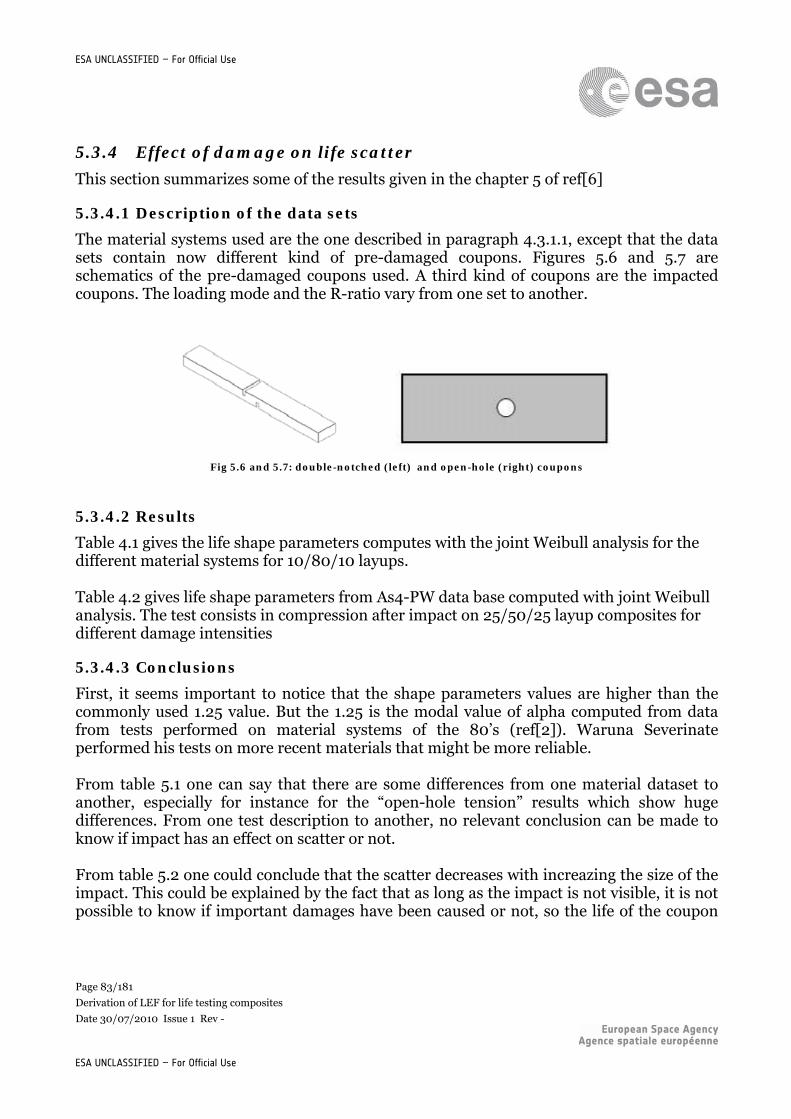
Page 83/181





5.3.4 Effect of damage on life scatter

This section summarizes some of the results given in the chapter 5 of ref[6]

5.3.4.1 Description of the data sets

The material systems used are the one described in paragraph 4.3.1.1, except that the data sets contain now different kind of pre-damaged coupons. Figures 5.6 and 5.7 are schematics of the pre-damaged coupons used. A third kind of coupons are the impacted coupons. The loading mode and the R-ratio vary from one set to another.

Fig 5.6 and 5.7: double-notched (left) and open-hole (right) coupons

5.3.4.2 Results

Table 4.1 gives the life shape parameters computes with the joint Weibull analysis for the different material systems for 10/80/10 layups. Table 4.2 gives life shape parameters from As4-PW data base computed with joint Weibull analysis. The test consists in compression after impact on 25/50/25 layup composites for different damage intensities

5.3.4.3 Conclusions

First, it seems important to notice that the shape parameters values are higher than the commonly used 1.25 value. But the 1.25 is the modal value of alpha computed from data from tests performed on material systems of the 80’s (ref[2]). Waruna Severinate performed his tests on more recent materials that might be more reliable. From table 5.1 one can say that there are some differences from one material dataset to another, especially for instance for the “open-hole tension” results which show huge differences. From one test description to another, no relevant conclusion can be made to know if impact has an effect on scatter or not. From table 5.2 one could conclude that the scatter decreases with increazing the size of the impact. This could be explained by the fact that as long as the impact is not visible, it is not possible to know if important damages have been caused or not, so the life of the coupon

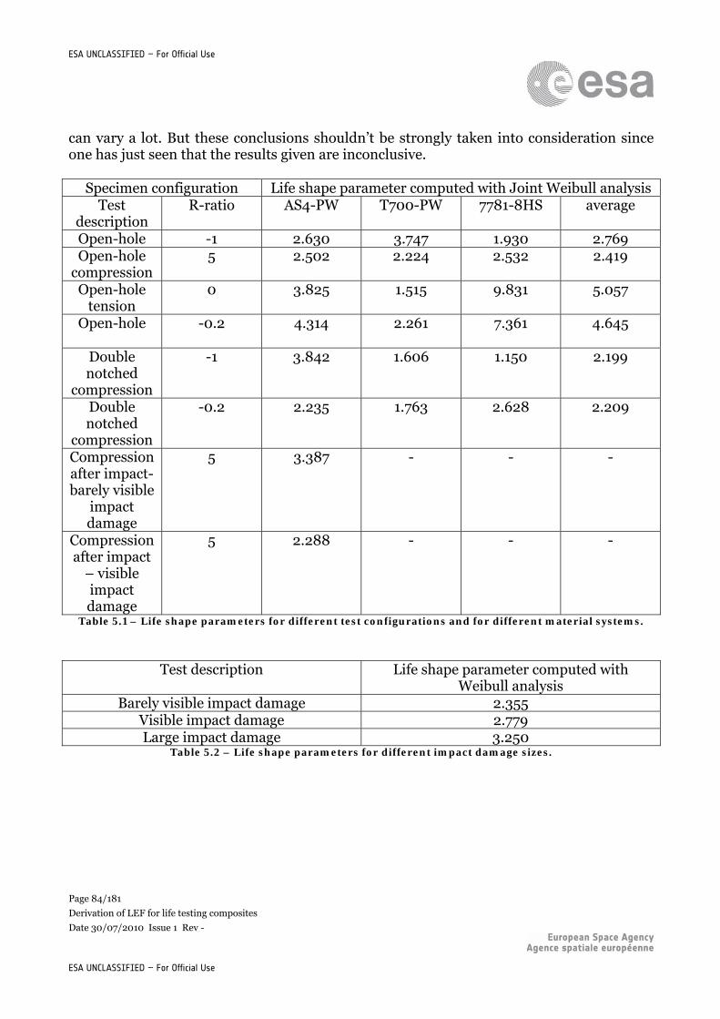
Page 84/181





can vary a lot. But these conclusions shouldn’t be strongly taken into consideration since one has just seen that the results given are inconclusive.

Specimen configuration Life shape parameter computed with Joint Weibull analysis Test

description R-ratio AS4-PW T700-PW 7781-8HS average

Open-hole -1 2.630 3.747 1.930 2.769 Open-hole

compression 5 2.502 2.224 2.532 2.419

Open-hole tension

0 3.825 1.515 9.831 5.057

Open-hole -0.2 4.314 2.261 7.361

4.645

Double notched

compression

-1 3.842 1.606 1.150 2.199

Double notched

compression

-0.2 2.235 1.763 2.628 2.209

Compression after impact-barely visible

impact damage

5 3.387 - - -

Compression after impact

– visible impact damage

5 2.288 - - -

Table 5.1 – Life shape parameters for different test configurations and for different material systems.

Test description Life shape parameter computed with Weibull analysis

Barely visible impact damage 2.355 Visible impact damage 2.779 Large impact damage 3.250

Table 5.2 – Life shape parameters for different impact damage sizes.

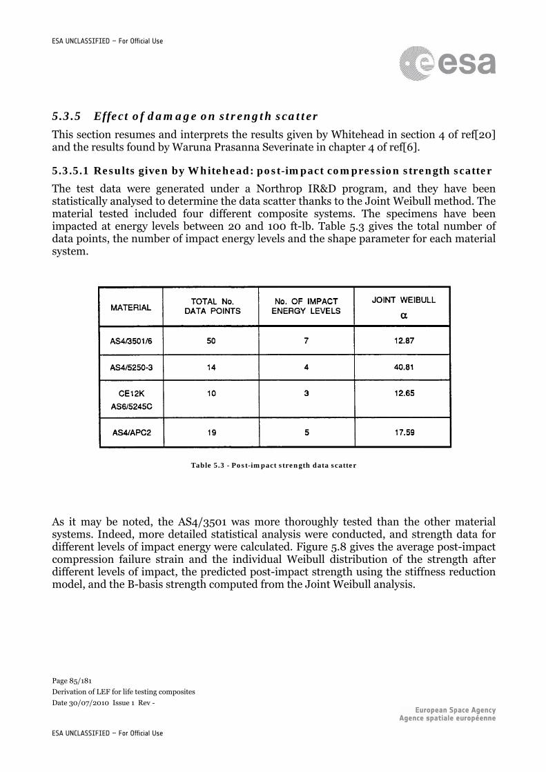
Page 85/181





5.3.5 Effect of damage on strength scatter

This section resumes and interprets the results given by Whitehead in section 4 of ref[20] and the results found by Waruna Prasanna Severinate in chapter 4 of ref[6].

5.3.5.1 Results given by Whitehead: post-impact compression strength scatter

The test data were generated under a Northrop IR&D program, and they have been statistically analysed to determine the data scatter thanks to the Joint Weibull method. The material tested included four different composite systems. The specimens have been impacted at energy levels between 20 and 100 ft-lb. Table 5.3 gives the total number of data points, the number of impact energy levels and the shape parameter for each material system.

Table 5.3 - Post-impact strength data scatter

As it may be noted, the AS4/3501 was more thoroughly tested than the other material systems. Indeed, more detailed statistical analysis were conducted, and strength data for different levels of impact energy were calculated. Figure 5.8 gives the average post-impact compression failure strain and the individual Weibull distribution of the strength after different levels of impact, the predicted post-impact strength using the stiffness reduction model, and the B-basis strength computed from the Joint Weibull analysis.

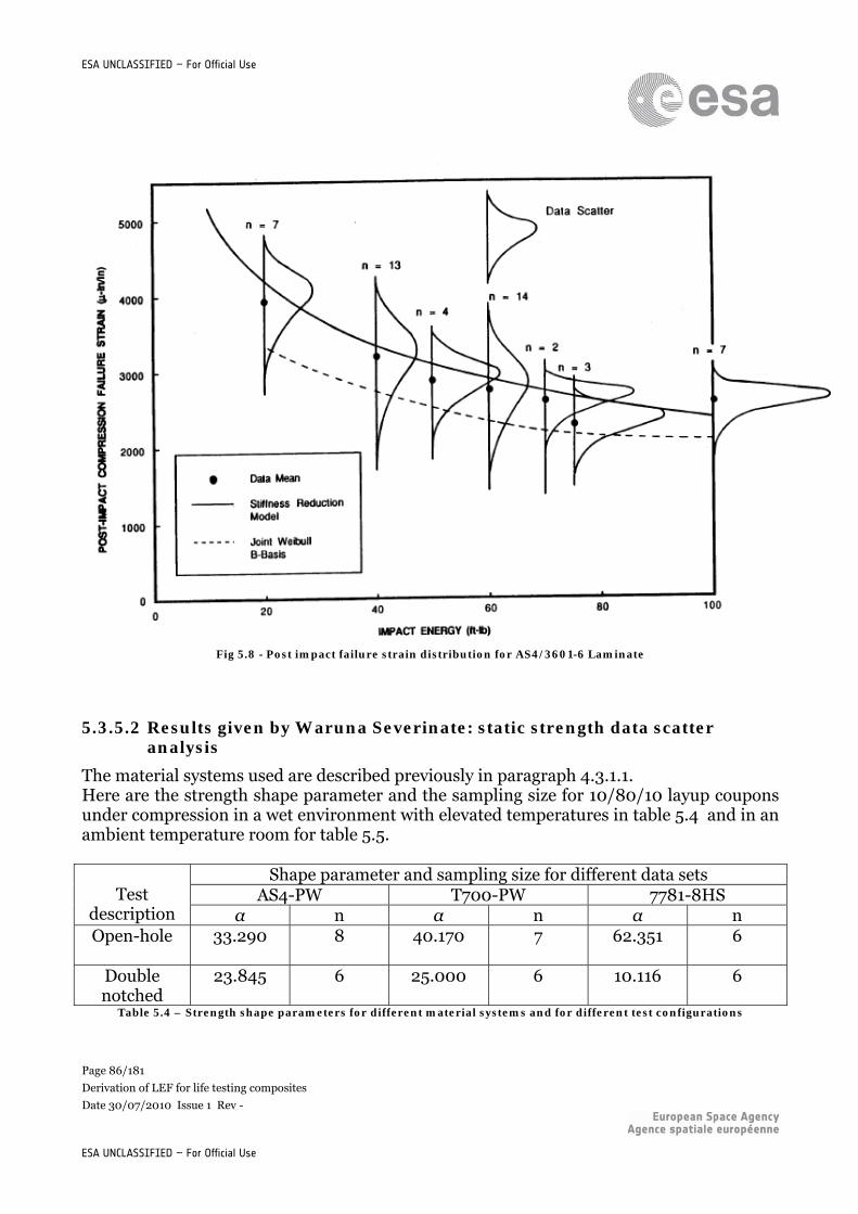
Page 86/181





Fig 5.8 - Post impact failure strain distribution for AS4/3601-6 Laminate

5.3.5.2 Results given by Waruna Severinate: static strength data scatter analysis

The material systems used are described previously in paragraph 4.3.1.1. Here are the strength shape parameter and the sampling size for 10/80/10 layup coupons under compression in a wet environment with elevated temperatures in table 5.4 and in an ambient temperature room for table 5.5.

Shape parameter and sampling size for different data sets AS4-PW T700-PW 7781-8HS

Test

description α n α n α n Open-hole

33.290 8 40.170 7 62.351 6

Double notched

23.845 6 25.000 6 10.116 6

Table 5.4 – Strength shape parameters for different material systems and for different test configurations

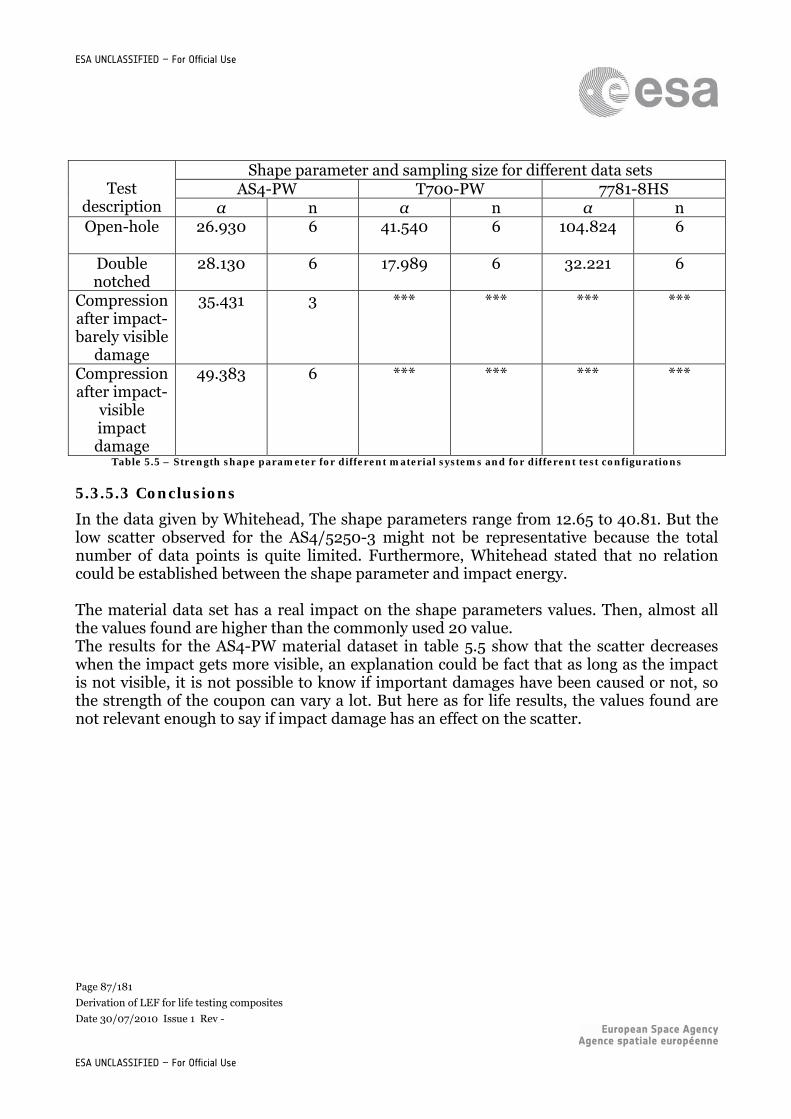
Page 87/181





Shape parameter and sampling size for different data sets

AS4-PW T700-PW 7781-8HS

Test description α n α n α n Open-hole

26.930 6 41.540 6 104.824 6

Double notched

28.130 6 17.989 6 32.221 6

Compression after impact-barely visible

damage

35.431 3 *** *** *** ***

Compression after impact-

visible impact damage

49.383 6 *** *** *** ***

Table 5.5 – Strength shape parameter for different material systems and for different test configurations

5.3.5.3 Conclusions

In the data given by Whitehead, The shape parameters range from 12.65 to 40.81. But the low scatter observed for the AS4/5250-3 might not be representative because the total number of data points is quite limited. Furthermore, Whitehead stated that no relation could be established between the shape parameter and impact energy. The material data set has a real impact on the shape parameters values. Then, almost all the values found are higher than the commonly used 20 value. The results for the AS4-PW material dataset in table 5.5 show that the scatter decreases when the impact gets more visible, an explanation could be fact that as long as the impact is not visible, it is not possible to know if important damages have been caused or not, so the strength of the coupon can vary a lot. But here as for life results, the values found are not relevant enough to say if impact damage has an effect on the scatter.

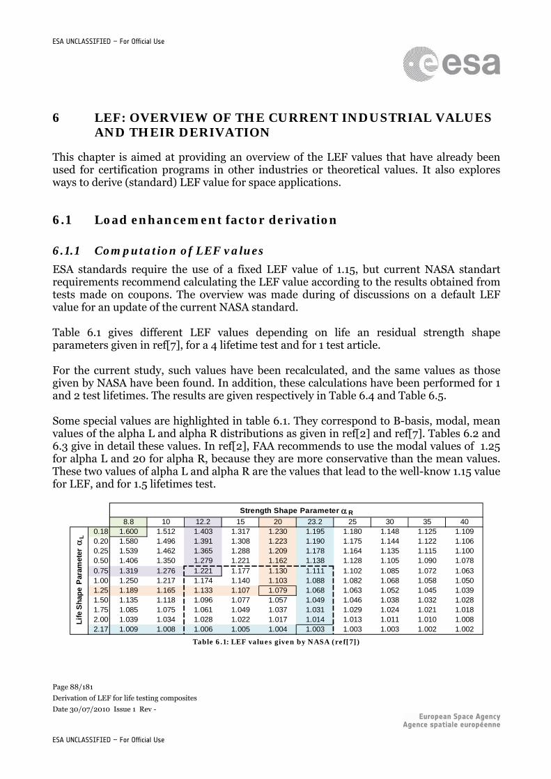
Page 88/181





6 LEF: OVERVIEW OF THE CURRENT INDUSTRIAL VALUES AND THEIR DERIVATION

This chapter is aimed at providing an overview of the LEF values that have already been used for certification programs in other industries or theoretical values. It also explores ways to derive (standard) LEF value for space applications.

6.1 Load enhancement factor derivation

6.1.1 Computation of LEF values

ESA standards require the use of a fixed LEF value of 1.15, but current NASA standart requirements recommend calculating the LEF value according to the results obtained from tests made on coupons. The overview was made during of discussions on a default LEF value for an update of the current NASA standard. Table 6.1 gives different LEF values depending on life an residual strength shape parameters given in ref[7], for a 4 lifetime test and for 1 test article. For the current study, such values have been recalculated, and the same values as those given by NASA have been found. In addition, these calculations have been performed for 1 and 2 test lifetimes. The results are given respectively in Table 6.4 and Table 6.5. Some special values are highlighted in table 6.1. They correspond to B-basis, modal, mean values of the alpha L and alpha R distributions as given in ref[2] and ref[7]. Tables 6.2 and 6.3 give in detail these values. In ref[2], FAA recommends to use the modal values of 1.25 for alpha L and 20 for alpha R, because they are more conservative than the mean values. These two values of alpha L and alpha R are the values that lead to the well-know 1.15 value for LEF, and for 1.5 lifetimes test.

8.8 10 12.2 15 20 23.2 25 30 35 400.18 1.600 1.512 1.403 1.317 1.230 1.195 1.180 1.148 1.125 1.1090.20 1.580 1.496 1.391 1.308 1.223 1.190 1.175 1.144 1.122 1.1060.25 1.539 1.462 1.365 1.288 1.209 1.178 1.164 1.135 1.115 1.1000.50 1.406 1.350 1.279 1.221 1.162 1.138 1.128 1.105 1.090 1.0780.75 1.319 1.276 1.221 1.177 1.130 1.111 1.102 1.085 1.072 1.0631.00 1.250 1.217 1.174 1.140 1.103 1.088 1.082 1.068 1.058 1.0501.25 1.189 1.165 1.133 1.107 1.079 1.068 1.063 1.052 1.045 1.0391.50 1.135 1.118 1.096 1.077 1.057 1.049 1.046 1.038 1.032 1.0281.75 1.085 1.075 1.061 1.049 1.037 1.031 1.029 1.024 1.021 1.0182.00 1.039 1.034 1.028 1.022 1.017 1.014 1.013 1.011 1.010 1.0082.17 1.009 1.008 1.006 1.005 1.004 1.003 1.003 1.003 1.002 1.002

Strength Shape Parameter R

Lif

e S

hap

e P

aram

eter

L

Table 6.1: LEF values given by NASA (ref[7])

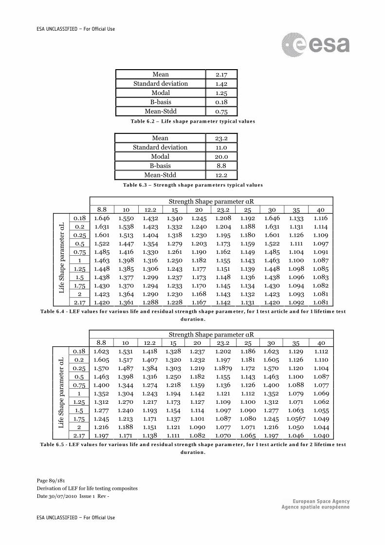
Page 89/181





Mean 2.17

Standard deviation 1.42

Modal 1.25

B-basis 0.18

Mean-Stdd 0.75

Table 6.2 – Life shape parameter typical values

Mean 23.2

Standard deviation 11.0

Modal 20.0

B-basis 8.8

Mean-Stdd 12.2

Table 6.3 – Strength shape parameters typical values

Strength Shape parameter αR 8.8 10 12.2 15 20 23.2 25 30 35 40

0.18 1.646 1.550 1.432 1.340 1.245 1.208 1.192 1.646 1.133 1.116 0.2 1.631 1.538 1.423 1.332 1.240 1.204 1.188 1.631 1.131 1.114

0.25 1.601 1.513 1.404 1.318 1.230 1.195 1.180 1.601 1.126 1.109 0.5 1.522 1.447 1.354 1.279 1.203 1.173 1.159 1.522 1.111 1.097

0.75 1.485 1.416 1.330 1.261 1.190 1.162 1.149 1.485 1.104 1.091 1 1.463 1.398 1.316 1.250 1.182 1.155 1.143 1.463 1.100 1.087

1.25 1.448 1.385 1.306 1.243 1.177 1.151 1.139 1.448 1.098 1.085 1.5 1.438 1.377 1.299 1.237 1.173 1.148 1.136 1.438 1.096 1.083

1.75 1.430 1.370 1.294 1.233 1.170 1.145 1.134 1.430 1.094 1.082 2 1.423 1.364 1.290 1.230 1.168 1.143 1.132 1.423 1.093 1.081 L

ife

Shap

e p

aram

eter

αL

2.17 1.420 1.361 1.288 1.228 1.167 1.142 1.131 1.420 1.092 1.081 Table 6.4 - LEF values for various life and residual strength shape parameter, for 1 test article and for 1 lifetime test

duration.

Strength Shape parameter αR 8.8 10 12.2 15 20 23.2 25 30 35 40

0.18 1.623 1.531 1.418 1.328 1.237 1.202 1.186 1.623 1.129 1.112 0.2 1.605 1.517 1.407 1.320 1.232 1.197 1.181 1.605 1.126 1.110

0.25 1.570 1.487 1.384 1.303 1.219 1.1879 1.172 1.570 1.120 1.104 0.5 1.463 1.398 1.316 1.250 1.182 1.155 1.143 1.463 1.100 1.087

0.75 1.400 1.344 1.274 1.218 1.159 1.136 1.126 1.400 1.088 1.077 1 1.352 1.304 1.243 1.194 1.142 1.121 1.112 1.352 1.079 1.069

1.25 1.312 1.270 1.217 1.173 1.127 1.109 1.100 1.312 1.071 1.062 1.5 1.277 1.240 1.193 1.154 1.114 1.097 1.090 1.277 1.063 1.055

1.75 1.245 1.213 1.171 1.137 1.101 1.087 1.080 1.245 1.0567 1.049 2 1.216 1.188 1.151 1.121 1.090 1.077 1.071 1.216 1.050 1.044 L

ife

Shap

e p

aram

eter

αL

2.17 1.197 1.171 1.138 1.111 1.082 1.070 1.065 1.197 1.046 1.040 Table 6.5 - LEF values for various life and residual strength shape parameter, for 1 test article and for 2 lifetime test

duration.

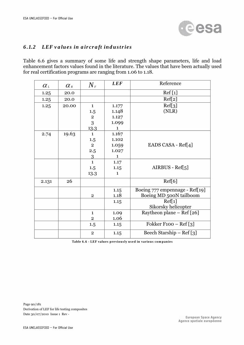
Page 90/181





6.1.2 LEF values in aircraft industries

Table 6.6 gives a summary of some life and strength shape parameters, life and load enhancement factors values found in the literature. The values that have been actually used for real certification programs are ranging from 1.06 to 1.18.

L R

N F LEF Reference

1.25 20.0 Ref [1] 1.25 20.0 Ref[2] 1.25 20.00 1

1.5 2 3

13.3

1.177 1.148 1.127 1.099

1

Ref[3] (NLR)

2.74 19.63 1 1.5 2

2.5 3

1.167 1.102 1.059 1.027

1

EADS CASA - Ref[4]

1 1.5

13.3

1.17 1.15

1

AIRBUS - Ref[5]

2.131 26 Ref[6]

2

1.15 1.18

Boeing 777 empennage - Ref[19] Boeing MD 500N tailboom

1.15 Ref[1] Sikorsky helicopter

1 2

1.09 1.06

Raytheon plane – Ref [26]

1.5 1.15 Fokker F100 – Ref [3]

2 1.15 Beech Starship – Ref [3]

Table 6.6 - LEF values previously used in various companies

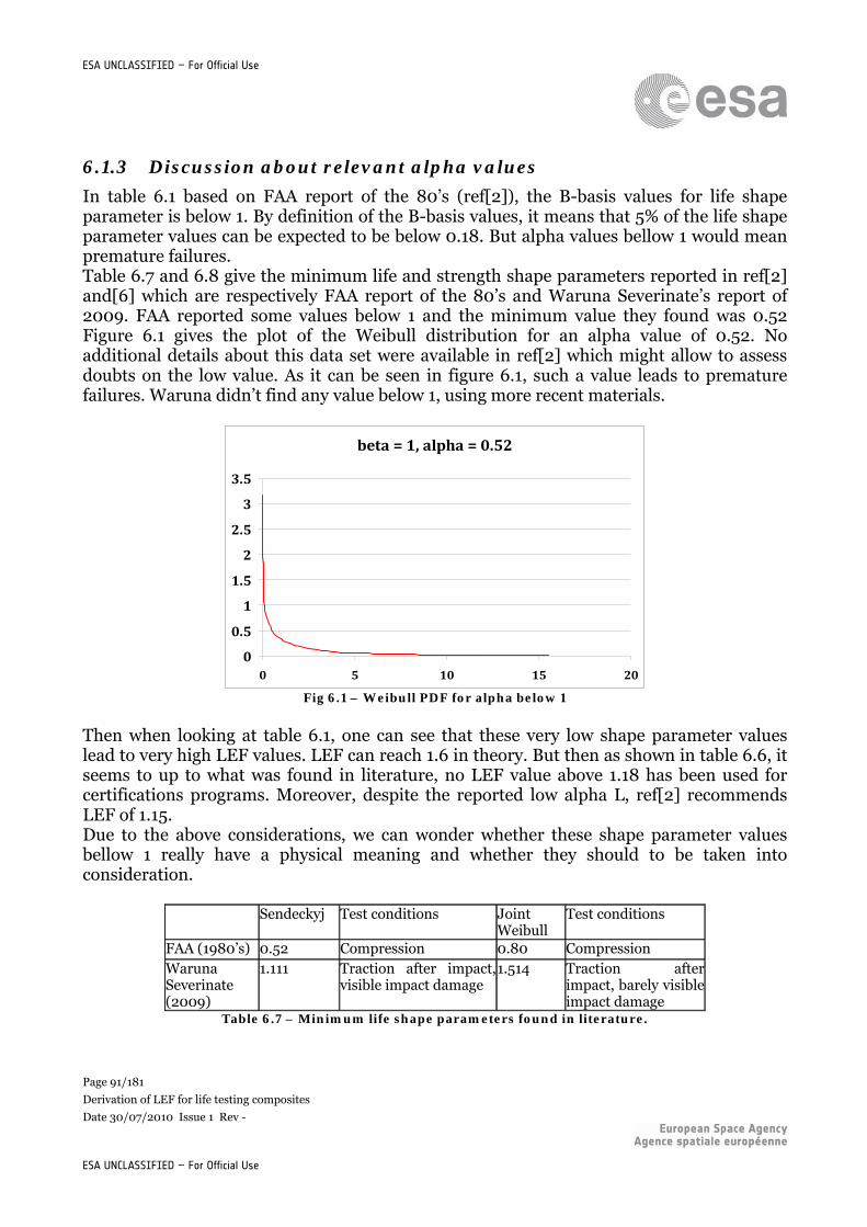
Page 91/181





6.1.3 Discussion about relevant alpha values

In table 6.1 based on FAA report of the 80’s (ref[2]), the B-basis values for life shape parameter is below 1. By definition of the B-basis values, it means that 5% of the life shape parameter values can be expected to be below 0.18. But alpha values bellow 1 would mean premature failures. Table 6.7 and 6.8 give the minimum life and strength shape parameters reported in ref[2] and[6] which are respectively FAA report of the 80’s and Waruna Severinate’s report of 2009. FAA reported some values below 1 and the minimum value they found was 0.52 Figure 6.1 gives the plot of the Weibull distribution for an alpha value of 0.52. No additional details about this data set were available in ref[2] which might allow to assess doubts on the low value. As it can be seen in figure 6.1, such a value leads to premature failures. Waruna didn’t find any value below 1, using more recent materials.

beta = 1, alpha = 0.52

0

0.5

1

1.5

2

2.5

3

3.5

0 5 10 15 20

Fig 6.1 – Weibull PDF for alpha below 1

Then when looking at table 6.1, one can see that these very low shape parameter values lead to very high LEF values. LEF can reach 1.6 in theory. But then as shown in table 6.6, it seems to up to what was found in literature, no LEF value above 1.18 has been used for certifications programs. Moreover, despite the reported low alpha L, ref[2] recommends LEF of 1.15. Due to the above considerations, we can wonder whether these shape parameter values bellow 1 really have a physical meaning and whether they should to be taken into consideration.

Sendeckyj Test conditions Joint Weibull

Test conditions

FAA (1980’s) 0.52 Compression 0.80 Compression Waruna Severinate (2009)

1.111 Traction after impact, visible impact damage

1.514 Traction after impact, barely visible impact damage

Table 6.7 – Minimum life shape parameters found in literature.

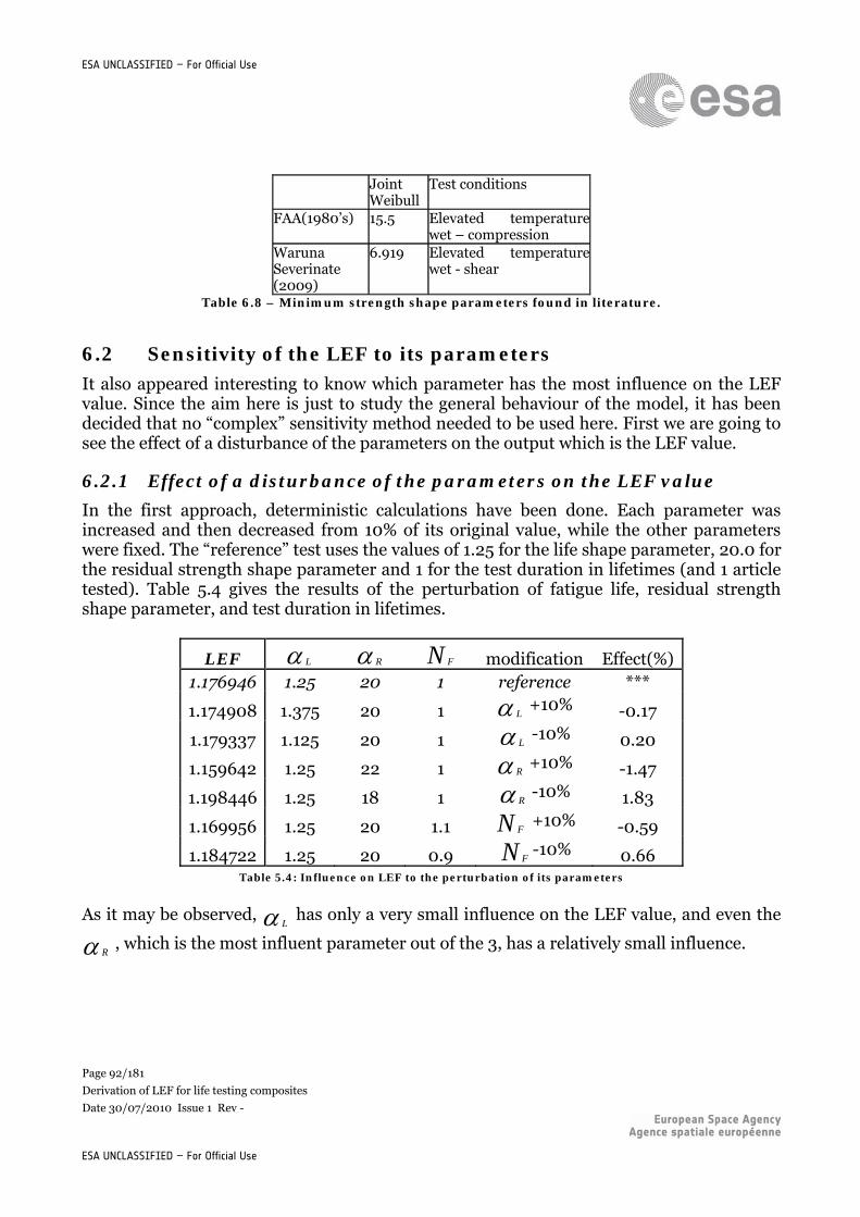
Page 92/181





Joint

Weibull Test conditions

FAA(1980’s) 15.5 Elevated temperature wet – compression

Waruna Severinate (2009)

6.919 Elevated temperature wet - shear

Table 6.8 – Minimum strength shape parameters found in literature.

6.2 Sensitivity of the LEF to its parameters

It also appeared interesting to know which parameter has the most influence on the LEF value. Since the aim here is just to study the general behaviour of the model, it has been decided that no “complex” sensitivity method needed to be used here. First we are going to see the effect of a disturbance of the parameters on the output which is the LEF value.

6.2.1 Effect of a disturbance of the parameters on the LEF value

In the first approach, deterministic calculations have been done. Each parameter was increased and then decreased from 10% of its original value, while the other parameters were fixed. The “reference” test uses the values of 1.25 for the life shape parameter, 20.0 for the residual strength shape parameter and 1 for the test duration in lifetimes (and 1 article tested). Table 5.4 gives the results of the perturbation of fatigue life, residual strength shape parameter, and test duration in lifetimes.

LEF L R

N F modification Effect(%)

1.176946 1.25 20 1 reference ***

1.174908 1.375 20 1 L +10% -0.17

1.179337 1.125 20 1 L -10% 0.20

1.159642 1.25 22 1 R +10% -1.47

1.198446 1.25 18 1 R -10% 1.83

1.169956 1.25 20 1.1 N F +10% -0.59

1.184722 1.25 20 0.9 N F-10% 0.66

Table 5.4: Influence on LEF to the perturbation of its parameters

As it may be observed, L has only a very small influence on the LEF value, and even the

R , which is the most influent parameter out of the 3, has a relatively small influence.

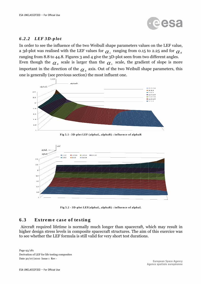
Page 93/181





6.2.2 LEF 3D-plot

In order to see the influence of the two Weibull shape parameters values on the LEF value, a 3d-plot was realised with the LEF values for L

ranging from 0.15 to 2.25 and for R

ranging from 8.8 to 44.8. Figures 3 and 4 give the 3D-plot seen from two different angles. Even though the R

scale is larger than the L scale, the gradient of slope is more

important in the direction of the R axis. Out of the two Weibull shape parameters, this

one is generally (see previous section) the most influent one.

Fig 5.1 - 3D-plot LEF (alphaL, alphaR) : influence of alphaR

Fig 5.2 - 3D-plot LEF(alphaL, alphaR) : influence of alphaL

6.3 Extreme case of testing

Aircraft required lifetime is normally much longer than spacecraft, which may result in higher design stress levels in composite spacecraft structures. The aim of this exercice was to see whether the LEF formula is still valid for very short test durations.

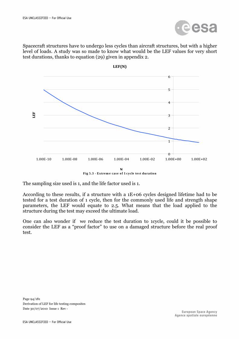
Page 94/181





Spacecraft structures have to undergo less cycles than aircraft structures, but with a higher level of loads. A study was so made to know what would be the LEF values for very short test durations, thanks to equation (29) given in appendix 2.

LEF(N)

0

1

2

3

4

5

6

1.00E‐10 1.00E‐08 1.00E‐06 1.00E‐04 1.00E‐02 1.00E+00 1.00E+02

N

LEF

Fig 5.3 - Extreme case of 1 cycle test duration

The sampling size used is 1, and the life factor used is 1. According to these results, if a structure with a 1E+06 cycles designed lifetime had to be tested for a test duration of 1 cycle, then for the commonly used life and strength shape parameters, the LEF would equate to 2.5. What means that the load applied to the structure during the test may exceed the ultimate load.

One can also wonder if we reduce the test duration to 1cycle, could it be possible to consider the LEF as a “proof factor” to use on a damaged structure before the real proof test.

Page 95/181





7 ASSESSMENT OF MAXIMUM ALLOWED MATERIAL SCATTER

7.1 General approach

The current NASA fracture control standard requires testing of coupons, specimen, subcomponents and components in order to derive the LEF to be used for full scale testing. The idea in this chapter is to think this process in the opposite way: if we want to have full scale testing with LEF=1.15 and n=1, and the shortest test duration as possible, what are the maximum scatter in strength and life that the material used has to prove?

7.2 Basic requirements

Starting from the LEF formula:

nnNp L

L

L

LEFR

RL

2)2(

)ln(

1

2

1

(7.a)

We can have an expression of the strength shape parameter as a function of all the other parameters. Trying to have an analytical expression of the life shape parameter as a function of the other parameters is difficult, because of the gamma function.

)ln(

)2ln()2(ln)ln(ln)ln(.1

ln.2

LEF

nnpNL

L

LL

R

(7.b)

And since the test should be such as

n=1 LEF=1.15

And since for A-basis values,

p=0.99 γ=0.95

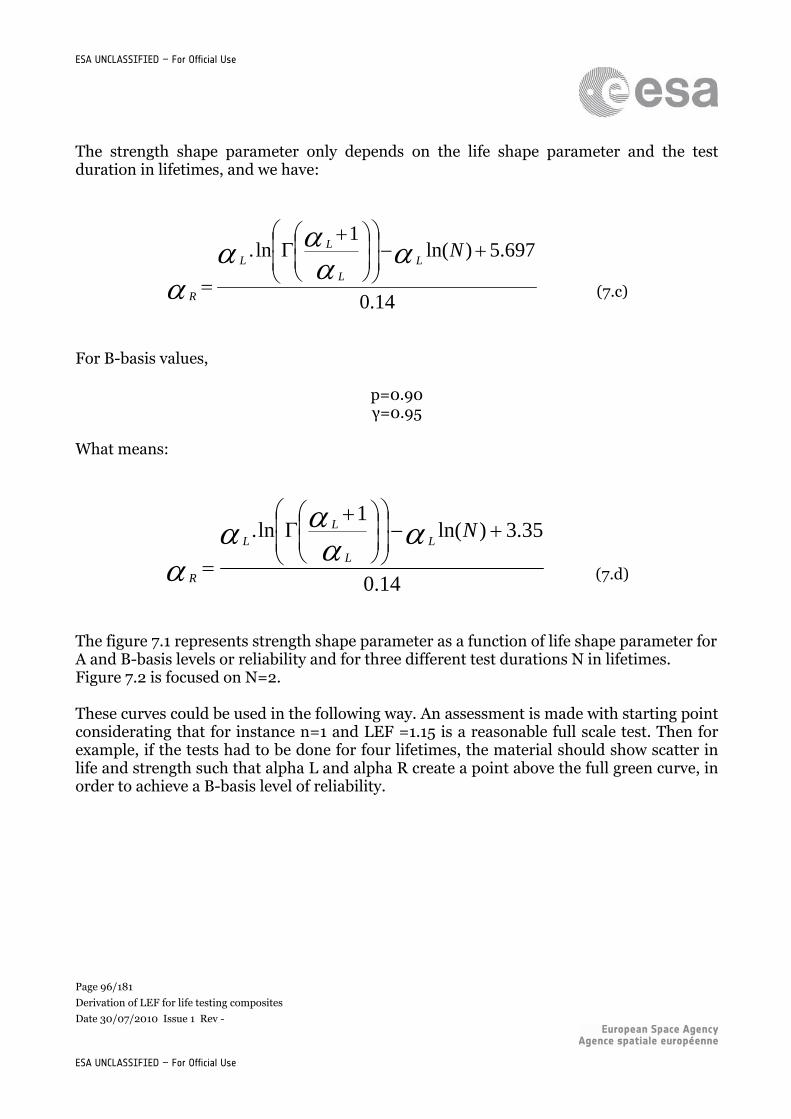
Page 96/181





The strength shape parameter only depends on the life shape parameter and the test duration in lifetimes, and we have:

14.0

697.5)ln(1

ln.

NL

L

L

L

R

(7.c)

For B-basis values,

p=0.90 γ=0.95

What means:

14.0

35.3)ln(1

ln.

NL

L

LL

R

(7.d)

The figure 7.1 represents strength shape parameter as a function of life shape parameter for A and B-basis levels or reliability and for three different test durations N in lifetimes. Figure 7.2 is focused on N=2. These curves could be used in the following way. An assessment is made with starting point considerating that for instance n=1 and LEF =1.15 is a reasonable full scale test. Then for example, if the tests had to be done for four lifetimes, the material should show scatter in life and strength such that alpha L and alpha R create a point above the full green curve, in order to achieve a B-basis level of reliability.

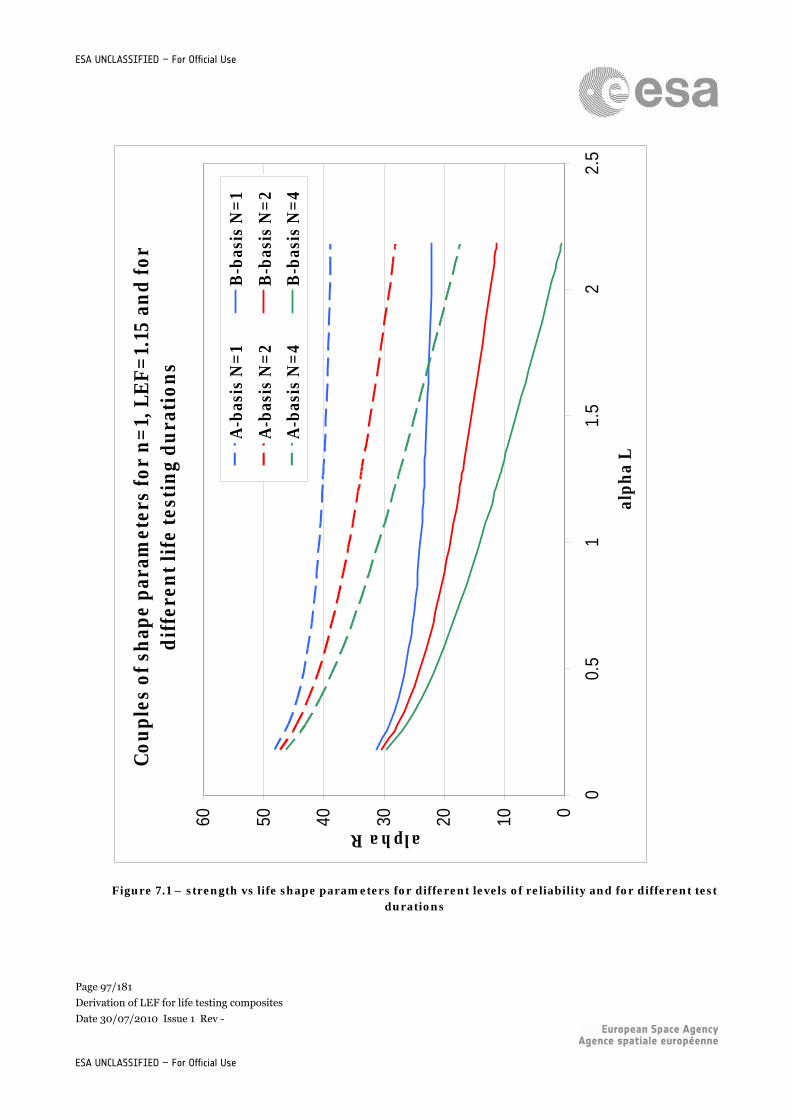
Page 97/181





Figure 7.1 – strength vs life shape parameters for different levels of reliability and for different test durations

Cou

ples

of s

hap

e pa

ram

eter

s fo

r n

=1,

LE

F=

1.15

an

d fo

r d

iffe

ren

t lif

e te

stin

g d

ura

tion

s

0102030405060

00.

51

1.5

22.

5

alp

ha

L

alpha R

A-b

asis

N=

1B

-bas

is N

=1

A-b

asis

N=

2B

-bas

is N

=2

A-b

asis

N=

4B

-bas

is N

=4

Page 98/181





Figure 7.2 – strength vs life shape parameters for different levels of reliability and for N=2

Co

up

les

of

shap

e p

aram

eter

s fo

r n

=1,

LE

F=

1.15

an

d f

or

dif

fere

nt

life

tes

tin

g d

ura

tio

ns

0102030405060

00.

51

1.5

22.

53

3.5

44.

5

alp

ha

L

alpha RA

-bas

is N

=2

B-b

asis

N=

2

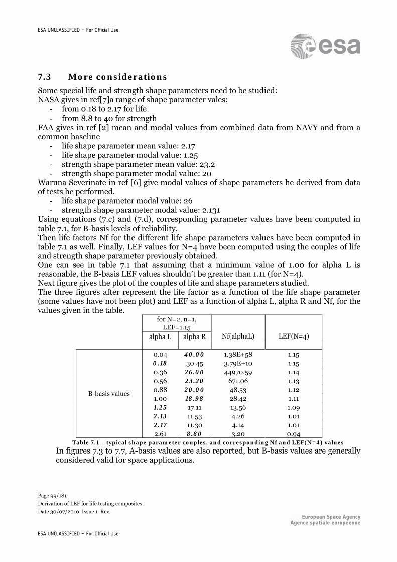
Page 99/181





7.3 More considerations

Some special life and strength shape parameters need to be studied: NASA gives in ref[7]a range of shape parameter vales:

- from 0.18 to 2.17 for life - from 8.8 to 40 for strength

FAA gives in ref [2] mean and modal values from combined data from NAVY and from a common baseline

- life shape parameter mean value: 2.17 - life shape parameter modal value: 1.25 - strength shape parameter mean value: 23.2 - strength shape parameter modal value: 20

Waruna Severinate in ref [6] give modal values of shape parameters he derived from data of tests he performed.

- life shape parameter modal value: 26 - strength shape parameter modal value: 2.131

Using equations (7.c) and (7.d), corresponding parameter values have been computed in table 7.1, for B-basis levels of reliability. Then life factors Nf for the different life shape parameters values have been computed in table 7.1 as well. Finally, LEF values for N=4 have been computed using the couples of life and strength shape parameter previously obtained. One can see in table 7.1 that assuming that a minimum value of 1.00 for alpha L is reasonable, the B-basis LEF values shouldn’t be greater than 1.11 (for N=4). Next figure gives the plot of the couples of life and shape parameters studied. The three figures after represent the life factor as a function of the life shape parameter (some values have not been plot) and LEF as a function of alpha L, alpha R and Nf, for the values given in the table.

for N=2, n=1,

LEF=1.15 alpha L alpha R Nf(alphaL) LEF(N=4)

0.04 40.00 1.38E+58 1.15 0.18 30.45 3.79E+10 1.15 0.36 26.00 44970.59 1.14 0.56 23.20 671.06 1.13 0.88 20.00 48.53 1.12 1.00 18.98 28.42 1.11 1.25 17.11 13.56 1.09 2.13 11.53 4.26 1.01 2.17 11.30 4.14 1.01

B-basis values

2.61 8.80 3.20 0.94 Table 7.1 – typical shape parameter couples, and corresponding Nf and LEF(N=4) values

In figures 7.3 to 7.7, A-basis values are also reported, but B-basis values are generally considered valid for space applications.

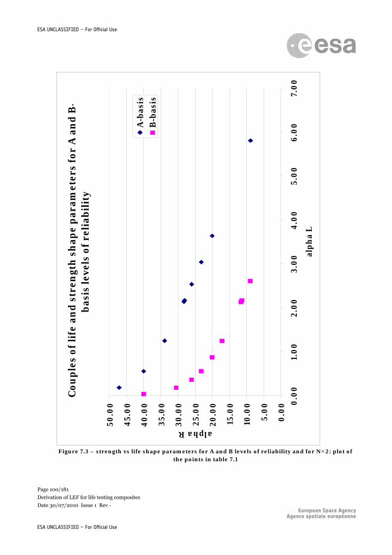
Page 100/181





Figure 7.3 – strength vs life shape parameters for A and B levels of reliability and for N=2: plot of

the points in table 7.1

Co

up

les

of

life

an

d s

tren

gth

sh

ape

par

amet

ers

for

A a

nd

B-

bas

is le

vels

of

reli

abil

ity

0.0

0

5.0

0

10.0

0

15.0

0

20

.00

25

.00

30

.00

35

.00

40

.00

45

.00

50

.00 0

.00

1.0

02

.00

3.0

04

.00

5.0

06

.00

7.0

0

alp

ha

L

alpha R

A-b

asis

B-b

asis

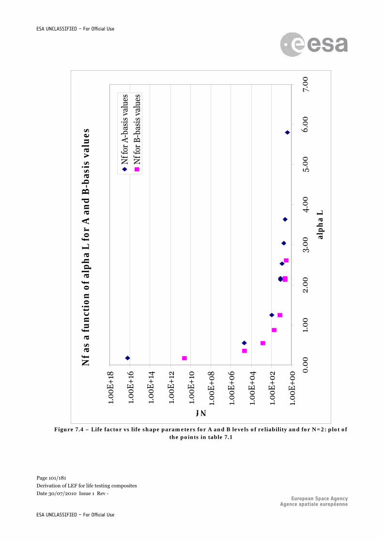
Page 101/181





Figure 7.4 – Life factor vs life shape parameters for A and B levels of reliability and for N=2: plot of


Nf

as a

fu

nct

ion

of

alp

ha

L f

or

A a

nd

B-b

asis

val

ues

1.00

E+

00

1.00

E+

02

1.00

E+

04

1.00

E+

06

1.00

E+

08

1.00

E+

10

1.00

E+

12

1.00

E+

14

1.00

E+

16

1.00

E+

18

0.00

1.00

2.00

3.00

4.00

5.00

6.00

7.00

alp

ha

L

NfN

f for

A-b

asis

val

ues

Nf f

or B

-bas

is v

alue

s

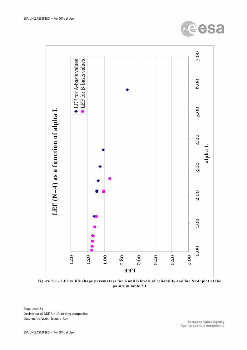
Page 102/181





Figure 7.5 – LEF vs life shape parameters for A and B levels of reliability and for N=4: plot of the

points in table 7.1

LE

F (

N=

4)

as a

fu

nct

ion

of

alp

ha

L

0.00

0.20

0.40

0.60

0.80

1.00

1.20

1.40

0.00

1.00

2.00

3.00

4.00

5.00

6.00

7.00

alp

ha

L

LEFLE

F fo

r A

-bas

is v

alue

sLE

F fo

r B

-bas

is v

alue

s

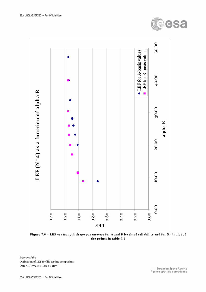
Page 103/181





Figure 7.6 – LEF vs strength shape parameters for A and B levels of reliability and for N=4: plot of


LE

F (

N=

4)

as a

fu

nct

ion

of

alp

ha

R

0.00

0.20

0.40

0.60

0.80

1.00

1.20

1.40

0.00

10.0

020

.00

30.0

040

.00

50.0

0

alp

ha

R

LEF

LEF

for

A-b

asis

val

ues

LEF

for

B-b

asis

val

ues

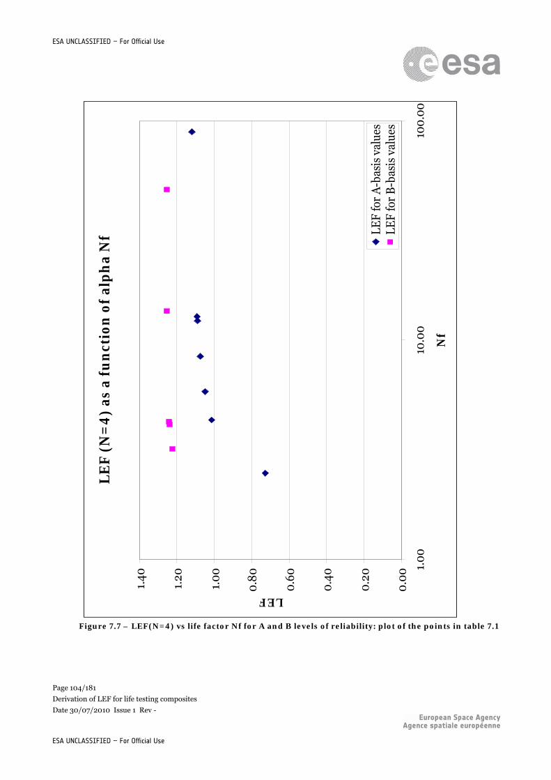
Page 104/181





Figure 7.7 – LEF(N=4) vs life factor Nf for A and B levels of reliability: plot of the points in table 7.1

LE

F (

N=

4)

as a

fu

nct

ion

of

alp

ha

Nf

0.00

0.20

0.40

0.60

0.80

1.00

1.20

1.40

1.00

10.0

010

0.00

Nf

LEF

LEF

for

A-b

asis

val

ues

LEF

for

B-b

asis

val

ues

Page 105/181





8 CONSIDERATIONS FOR CHOOSING A LEF DEFAULT VALUE

8.1 Probabilistic background

8.1.1 General reliability problem

In various applications, variables are not deterministic variables, but they are actually random variables, also called stochastic variables. It can be mathematically and conceptually helpful to assemble these random variables X i

(with i = 1, 2, …, n ) into a

random vector:

XXX nXt

,...,, 21 (8.a)

The main issue of a reliability analysis is the computation of the probability if failure, which is usually defined by:

0)(

)(xg

Xfxdxfp (8.b)

Where f

X is the joint density function of the random vector variable and g(X) is the limit

state function of the considered system. The possibility to have to deal with a high number of stochastic variables and sometimes the complexity of the integration domain make that generally, the solution can be achieved only by means of simulation methods.

8.1.2 Monte Carlo Simulation Method

The Monte Carlo simulation is one of the numerous methods of simulation, and it is surely the most widely known one. The Monte Carlo simulation is the art of approximating an expectation by sample method of a function of simulated random variables. In the direct Monte Carlo simulation, for solving multidimensional integrals, the integration domain in equation (previous one) is replaced by an indicator function:

Page 106/181





0)(0

0)(1)(

xg

xgxgI (8.c)

Which corresponds to a redefinition of the failure probability as the expected value of )(xgI , the so-called indicator function.

The equation (8.b) becomes then:

R

XgIxdxxgIn

Efp fXf)()( (8.d)

where the indice f refers to the joint density f

X.

With this redefinition, the random variables can be simulated according to their distribution, the indicator function can be evaluated from the limit state condition and the probability of failure can be finally estimated as:

NNx

Np

SIM

failure

ii

SIMf

NgI

SIM

1

1 (8.e)

Where: NSIM is the total number of simulations

N failure is the total number of failure

When the performance function is known, the Monte Carlo Simulation Method consists in the following steps:

Given the predefined PDF of the stochastic variables in the performance function, generate single values for each variable.

Evaluate the performance function: if 0xg , the system reached the failure domain.

Repeat the two former steps N SIM times.

Estimate the probability of failure using equation (8.e)

Page 107/181





8.2 Finite Element Reliability Using Matlab (FERUM)

FERUM (Finite Element Using Reliability) is an open-source Matlab toolbox initiated in 1999 in the University of California of Berckeley. It is now still developed in IFMA (French Institute for Advanced Mechanics). It is used in this section to perform the simulations needed.

8.3 Reliability analysis: choosing a LEF default value

The aim of this study is the following: given a LEF default value, a sampling size and a test duration in life times, what is the probability that my test achieves the B-basis level of reliability?

8.3.1 Definition of the problem

This problem has five variables: n, N, D, L and R

8.3.1.1 Deterministic variables

n: the sampling size. Since we are dealing with full scale testing, the sampling size is deterministic and equates to 1.

N: the test duration in lifetimes. This variable is also deterministic. For ESA, N=1, for NASA, N=4, for airbus and boeing, N=1.5. We are therefore going to run the simulations for N=1, N=1.5, N=2 and N=4.

D: the LEF default value This variable is deterministic. The simulations will be run for different specific LEF values ranging from 1 to 1.4.

8.3.1.2 Random variables

In ref [2], data given by the NAVY and the common baseline are analysed. According to ref [2], these data show that the Weibull life and strength shape parameters both follow again a Weibull distribution. Here is the description of the two random variables given in ref[2] and used by the NASA in ref[7]

R: the strength shape parameter

In ref [2], the data from navy and from a common baseline were first separately analysed, then they were all combined. The results of the combined data will be used here:

Mean = 23.2 Standard deviation = 11

L: the life shape parameter

Here again, ref[2] gives data from the navy and from a common baseline, but the combined data results are used for the current study:

Mean = 2.17 Standard deviation = 1.42

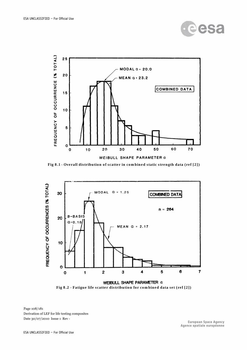
Page 108/181





Fig 8.1 - Overall distribution of scatter in combined static strength data (ref [2])

Fig 8.2 - Fatigue life scatter distribution for combined data set (ref [2])

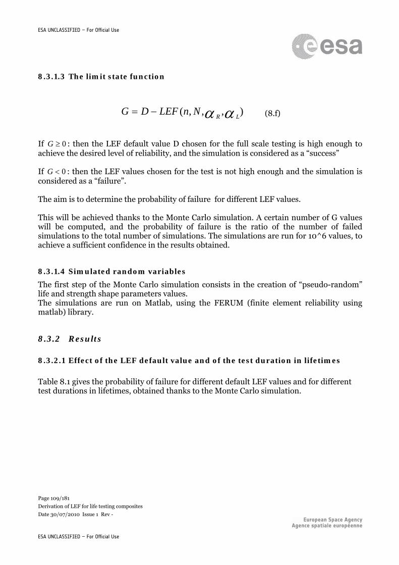
Page 109/181





8.3.1.3 The limit state function

),,,( LRNnLEFDG (8.f)

If 0G : then the LEF default value D chosen for the full scale testing is high enough to achieve the desired level of reliability, and the simulation is considered as a “success” If 0G : then the LEF values chosen for the test is not high enough and the simulation is considered as a “failure”. The aim is to determine the probability of failure for different LEF values. This will be achieved thanks to the Monte Carlo simulation. A certain number of G values will be computed, and the probability of failure is the ratio of the number of failed simulations to the total number of simulations. The simulations are run for 10^6 values, to achieve a sufficient confidence in the results obtained.

8.3.1.4 Simulated random variables

The first step of the Monte Carlo simulation consists in the creation of “pseudo-random” life and strength shape parameters values. The simulations are run on Matlab, using the FERUM (finite element reliability using matlab) library.

8.3.2 Results

8.3.2.1 Effect of the LEF default value and of the test duration in lifetimes

Table 8.1 gives the probability of failure for different default LEF values and for different test durations in lifetimes, obtained thanks to the Monte Carlo simulation.

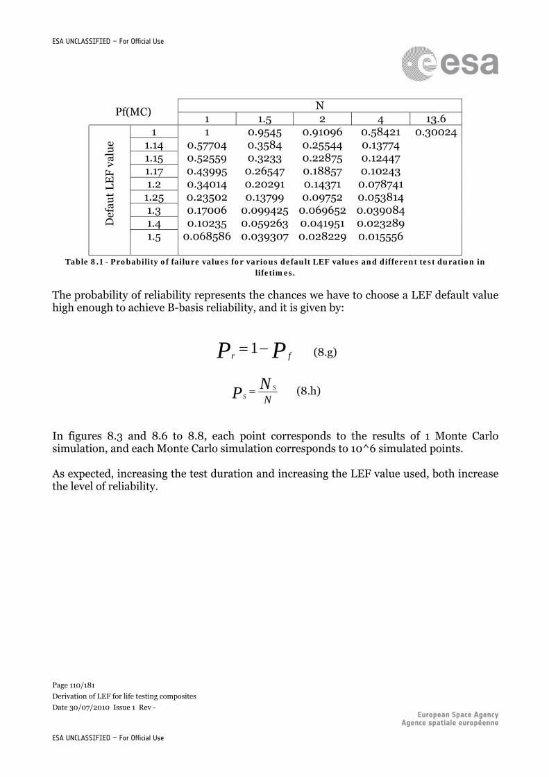
Page 110/181





N Pf(MC)

1 1.5 2 4 13.6 1 1 0.9545 0.91096 0.58421 0.30024

1.14 0.57704 0.3584 0.25544 0.13774 1.15 0.52559 0.3233 0.22875 0.12447 1.17 0.43995 0.26547 0.18857 0.10243 1.2 0.34014 0.20291 0.14371 0.078741

1.25 0.23502 0.13799 0.09752 0.053814 1.3 0.17006 0.099425 0.069652 0.039084 1.4 0.10235 0.059263 0.041951 0.023289 D

efau

t L

EF

val

ue

1.5 0.068586 0.039307 0.028229 0.015556

Table 8.1 - Probability of failure values for various default LEF values and different test duration in lifetimes.

The probability of reliability represents the chances we have to choose a LEF default value high enough to achieve B-basis reliability, and it is given by:

PP fr 1 (8.g)

NN

P S

S (8.h)

In figures 8.3 and 8.6 to 8.8, each point corresponds to the results of 1 Monte Carlo simulation, and each Monte Carlo simulation corresponds to 10^6 simulated points. As expected, increasing the test duration and increasing the LEF value used, both increase the level of reliability.

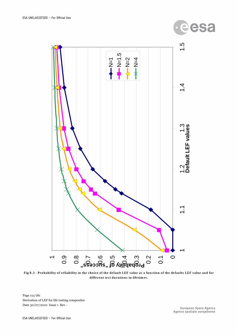
Page 111/181





Fig 8.3 - Probability of reliability in the choice of the default LEF value as a function of the defaults LEF value and for

different test durations in lifetimes.

0

0.1

0.2

0.3

0.4

0.5

0.6

0.7

0.8

0.91

11.

11.

21.

31.

41.

5D

efau

lt L

EF

val

ues

Probability of "success"

N=1

N=1

.5

N=2

N=4

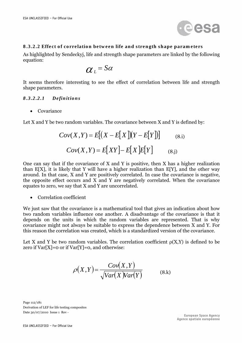
Page 112/181





8.3.2.2 Effect of correlation between life and strength shape parameters

As highlighted by Sendeckyj, life and strength shape parameters are linked by the following equation: It seems therefore interesting to see the effect of correlation between life and strength shape parameters.

8.3.2.2.1 Definitions

Covariance

Let X and Y be two random variables. The covariance between X and Y is defined by:

YEYXEXEYXCov ),( (8.i)

YEXEXYEYXCov ),( (8.j) One can say that if the covariance of X and Y is positive, then X has a higher realization than E[X], it is likely that Y will have a higher realization than E[Y], and the other way around. In that case, X and Y are positively correlated. In case the covariance is negative, the opposite effect occurs and X and Y are negatively correlated. When the covariance equates to zero, we say that X and Y are uncorrelated.

Correlation coefficient We just saw that the covariance is a mathematical tool that gives an indication about how two random variables influence one another. A disadvantage of the covariance is that it depends on the units in which the random variables are represented. That is why covariance might not always be suitable to express the dependence between X and Y. For this reason the correlation was created, which is a standardized version of the covariance. Let X and Y be two random variables. The correlation coefficient ρ(X,Y) is defined to be zero if Var[X]=0 or if Var[Y]=0, and otherwise:

YVarXVar

YXCovYX

,, (8.k)

SL

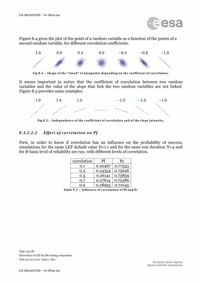
Page 113/181





Figure 8.4 gives the plot of the point of a random variable as a function of the points of a second random variable, for different correlation coefficients.

Fig 8.4 – Shape of the “cloud” of datapoints depending on the coefficient of correlation.

It seems important to notice that the coefficient of correlation between two random variables and the value of the slope that link the two random variables are not linked. Figure 8.5 provides some examples.

Fig 8.5 – Independence of the coefficient of correlation and of the slope intensity.

8.3.2.2.2 Effect of correlation on Pf

First, in order to know if correlation has an influence on the probability of success, simulations for the same LEF default value D=1.1 and for the same test duration N=4 and for B-basis level of reliability are run, with different levels of correlation.

correlation Pf Ps 0.1 0.22467 0.77533 0.3 0.24354 0.75646 0.5 0.26141 0.73859 0.7 0.27614 0.72386 0.9 0.28955 0.71045

Table 8.2 – Influence of correlation of Pf and Ps

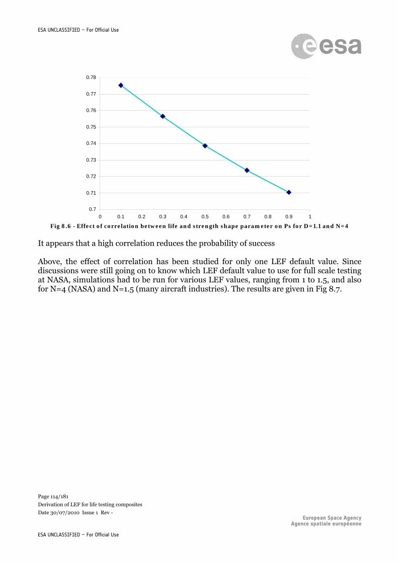
Page 114/181





0.7

0.71

0.72

0.73

0.74

0.75

0.76

0.77

0.78

0 0.1 0.2 0.3 0.4 0.5 0.6 0.7 0.8 0.9 1 Fig 8.6 - Effect of correlation between life and strength shape parameter on Ps for D=1.1 and N=4

It appears that a high correlation reduces the probability of success Above, the effect of correlation has been studied for only one LEF default value. Since discussions were still going on to know which LEF default value to use for full scale testing at NASA, simulations had to be run for various LEF values, ranging from 1 to 1.5, and also for N=4 (NASA) and N=1.5 (many aircraft industries). The results are given in Fig 8.7.

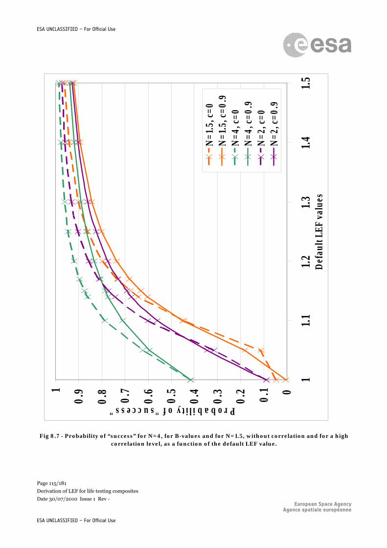
Page 115/181





Fig 8.7 - Probability of “success” for N=4, for B-values and for N=1.5, without correlation and for a high correlation level, as a function of the default LEF value.

0

0.1

0.2

0.3

0.4

0.5

0.6

0.7

0.8

0.91

11.

11.

21.

31.

41.

5D

efau

lt LE

F va

lues


N=1

.5, c

=0N

=1.5

, c=0

.9N

=4, c

=0N

=4, c

=0.9

N=2

, c=0

N=2

, c=0

.9

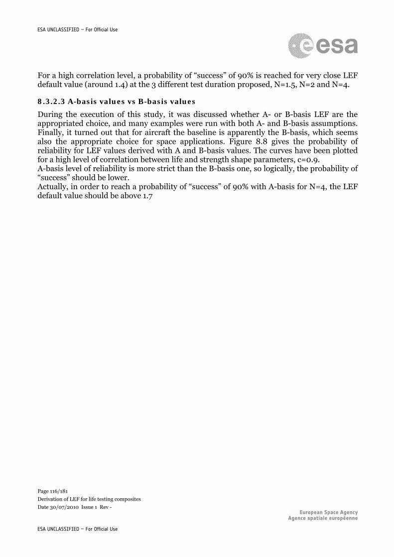
Page 116/181





For a high correlation level, a probability of “success” of 90% is reached for very close LEF default value (around 1.4) at the 3 different test duration proposed, N=1.5, N=2 and N=4.

8.3.2.3 A-basis values vs B-basis values

During the execution of this study, it was discussed whether A- or B-basis LEF are the appropriated choice, and many examples were run with both A- and B-basis assumptions. Finally, it turned out that for aircraft the baseline is apparently the B-basis, which seems also the appropriate choice for space applications. Figure 8.8 gives the probability of reliability for LEF values derived with A and B-basis values. The curves have been plotted for a high level of correlation between life and strength shape parameters, c=0.9. A-basis level of reliability is more strict than the B-basis one, so logically, the probability of “success” should be lower. Actually, in order to reach a probability of “success” of 90% with A-basis for N=4, the LEF default value should be above 1.7

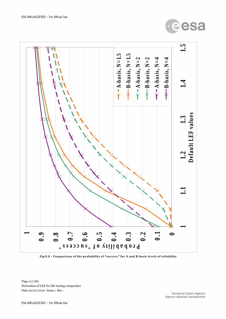
Page 117/181





Fig 8.8 - Comparison of the probability of “success” for A and B-basis levels of reliability

0

0.1

0.2

0.3

0.4

0.5

0.6

0.7

0.8

0.91

11.

11.

21.

31.

41.

5D

efau

lt L

EF

valu

es


A-b

asis

, N=1

.5

B-b

asis

, N=1

.5

A-b

asis

, N=2

B-b

asis

, N=2

A-b

asis

, N=4

B-b

asis

, N=4

Page 118/181





8.4 Interpretations discussions and conclusions

The aim of these simulations was not to choose a LEF value and a test duration that provide a certain probability of “success”, since we don’t have any order of magnitude of what could a right probability of “success” be for this application. But we know that some certification programs in aeroplane industry performed with a LEF value of 1.15 and for test durations of 1.5 lives were successful. Then it also seems that NASA is very interested in the couple of values of 1.1 for LEF and 4 for the test duration. The idea would be to choose a LEF value and a test duration that provide at least the same probability of “success” that the airplane values and the NASA values provide. For a high coefficient of correlation (c=0.9) and for a LEF of 1.1 and a test duration of 4 lifetimes (NASA), the probability of success achieved is 72% (see figure 8.7). And for a LEF of 1.15 and a test duration of 1.5 (airplane industry), the probability of success achieved is 64%. What also has to be mentioned is that the relevance of the distributions of alpha L and alpha R derived from the data obtained in the 1980’s is not clear.

Page 119/181





9 WARUNA’S DATA NALYSIS

9.1 Available data

The fatigue life and strength data available in literature are Waruna Severinate’s S-N test data (in appendix of ref[6]). The author tested coupons made of AS4-PW material, for different layup configurations, different test configurations and different loading modes. The data and the corresponding S-N plot are given in appendix 4.

9.2 Easyfit software

The software used for the analysis performed for the this report is the statistical software Easyfit. For a given set of data containing at least 5 points, it searches the best parameters to fit 61 implemented distributions. It can also provide a plot of the PDF (probability density function), the CDF(cumulative density function), the hazard function of all the fitted distributions compared to the real data points given as histograms. It can also provide the results of 3 different goodness of fit tests: Kolmogorov-Smirnov, Chi-square and Anderson-Darling (see sections 1.3.5.14 to 1.3.5.16 in ref[27]). The software is first used to compute the Weibull parameters of the data and compare them to Waruna’s results. Then ref[2] assumes that the Weibull distribution is the best fit. The easyfit software will be used to compare the fit of the 61 distributions implemented on one example of set of data in strength and another one in fatigue, and thanks to the goodness of fit tests implemented it will be possible to compare the quality of the fit made on every distribution, to know which one is the “best”. Then the software will also be used to see the influence of the weibull shape and scale parameter on the quality of the fit. And finally, it will also be used to find the best fit of the distribution on the alpha values, to know the alpha distribution for the reliability analysis (see chapter 8).

9.3 Statistical analysis

9.3.1 Strength data

The strength data are the test results for which n=1. The coupons are loaded until failure and the stress level at failure is the static strength of the material. Only the data containing at least the results on 5 coupons are taken into account, because of the Easyfit software requirements. Ref[2] recommends to use the 2-parameter Weibull distribution for fitting the data, so, for every batch, the scale and shape parameters of the most representative Weibull distribution have been computed using the individual Weibull method (Classical maximum likelihood estimation). Shape and scale parameter are derived using the two following formulas that have to be solved using iterative schemes:

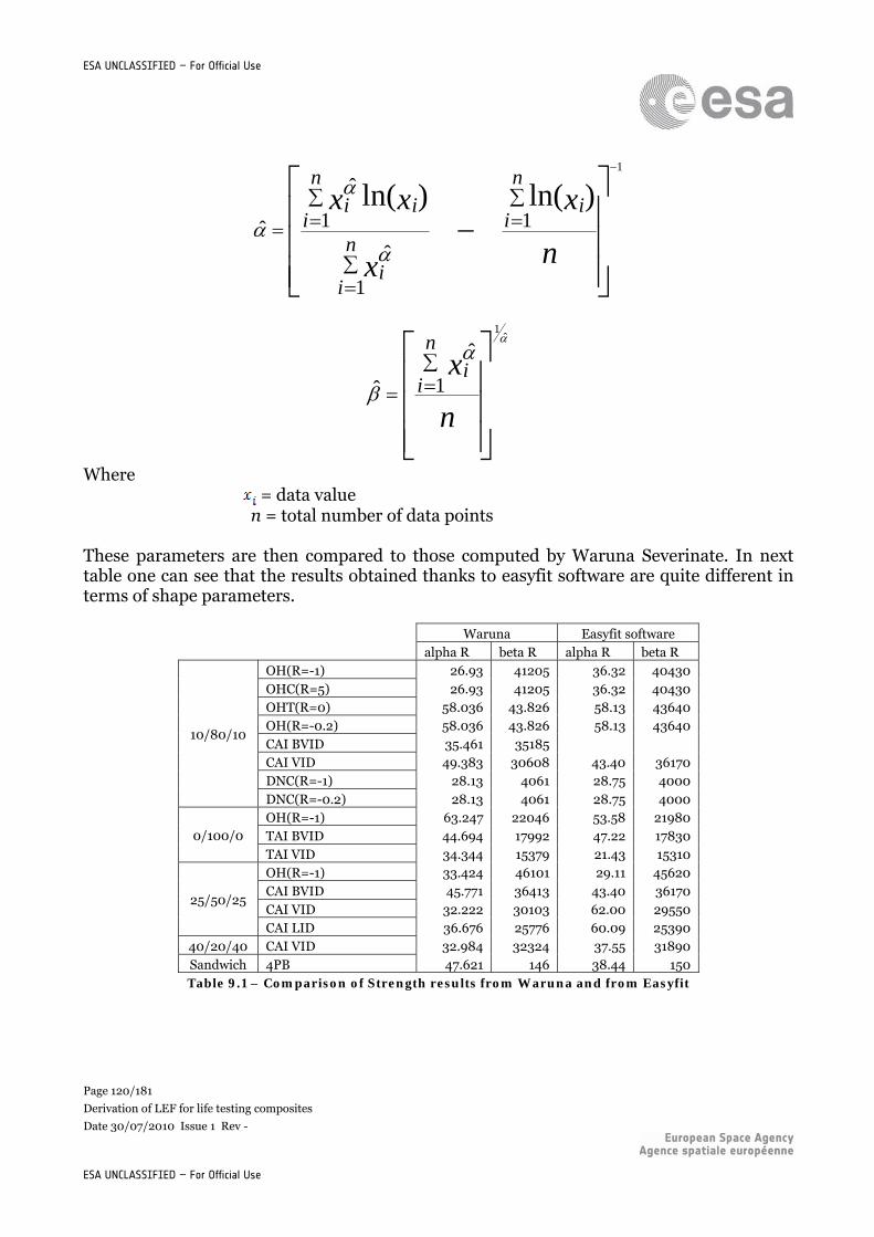
Page 120/181





n

x

x

xxn

ii

n

ii

n

iii

1

1

ˆ

1

ˆ

ˆ

)ln()ln(1

n

xn

ii

1

ˆ

ˆ

ˆ1

Where = data value

n = total number of data points These parameters are then compared to those computed by Waruna Severinate. In next table one can see that the results obtained thanks to easyfit software are quite different in terms of shape parameters.

Waruna Easyfit software alpha R beta R alpha R beta R

OH(R=-1) 26.93 41205 36.32 40430 OHC(R=5) 26.93 41205 36.32 40430 OHT(R=0) 58.036 43.826 58.13 43640 OH(R=-0.2) 58.036 43.826 58.13 43640 CAI BVID 35.461 35185 CAI VID 49.383 30608 43.40 36170 DNC(R=-1) 28.13 4061 28.75 4000

10/80/10

DNC(R=-0.2) 28.13 4061 28.75 4000 OH(R=-1) 63.247 22046 53.58 21980 TAI BVID 44.694 17992 47.22 17830 0/100/0

TAI VID 34.344 15379 21.43 15310 OH(R=-1) 33.424 46101 29.11 45620 CAI BVID 45.771 36413 43.40 36170 CAI VID 32.222 30103 62.00 29550

25/50/25

CAI LID 36.676 25776 60.09 25390 40/20/40 CAI VID 32.984 32324 37.55 31890 Sandwich 4PB 47.621 146 38.44 150 Table 9.1 – Comparison of Strength results from Waruna and from Easyfit

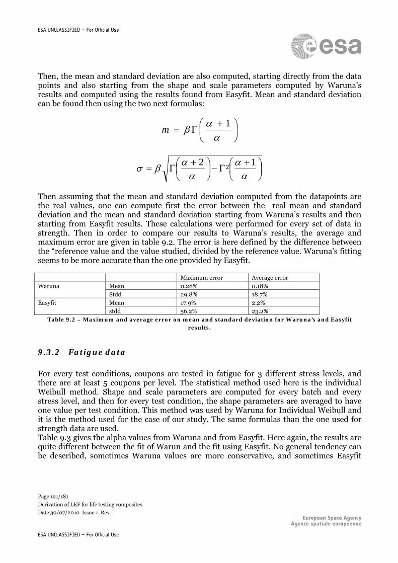
Page 121/181





Then, the mean and standard deviation are also computed, starting directly from the data points and also starting from the shape and scale parameters computed by Waruna’s results and computed using the results found from Easyfit. Mean and standard deviation can be found then using the two next formulas:

1m

1²

2

Then assuming that the mean and standard deviation computed from the datapoints are the real values, one can compute first the error between the real mean and standard deviation and the mean and standard deviation starting from Waruna’s results and then starting from Easyfit results. These calculations were performed for every set of data in strength. Then in order to compare our results to Waruna’s results, the average and maximum error are given in table 9.2. The error is here defined by the difference between the “reference value and the value studied, divided by the reference value. Waruna’s fitting seems to be more accurate than the one provided by Easyfit. Maximum error Average error

Mean 0.28% 0.18% Waruna Stdd 29.8% 18.7% Mean 17.9% 2.2% Easyfit stdd 56.2% 23.2%

Table 9.2 – Maximum and average error on mean and standard deviation for Waruna’s and Easyfit results.

9.3.2 Fatigue data

For every test conditions, coupons are tested in fatigue for 3 different stress levels, and there are at least 5 coupons per level. The statistical method used here is the individual Weibull method. Shape and scale parameters are computed for every batch and every stress level, and then for every test condition, the shape parameters are averaged to have one value per test condition. This method was used by Waruna for Individual Weibull and it is the method used for the case of our study. The same formulas than the one used for strength data are used. Table 9.3 gives the alpha values from Waruna and from Easyfit. Here again, the results are quite different between the fit of Warun and the fit using Easyfit. No general tendency can be described, sometimes Waruna values are more conservative, and sometimes Easyfit

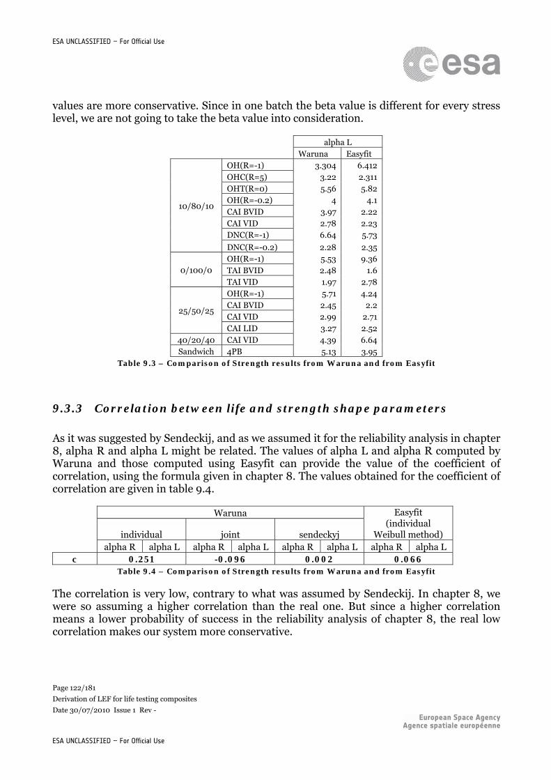
Page 122/181





values are more conservative. Since in one batch the beta value is different for every stress level, we are not going to take the beta value into consideration.

alpha L Waruna Easyfit

OH(R=-1) 3.304 6.412 OHC(R=5) 3.22 2.311 OHT(R=0) 5.56 5.82 OH(R=-0.2) 4 4.1 CAI BVID 3.97 2.22 CAI VID 2.78 2.23 DNC(R=-1) 6.64 5.73

10/80/10

DNC(R=-0.2) 2.28 2.35 OH(R=-1) 5.53 9.36 TAI BVID 2.48 1.6 0/100/0

TAI VID 1.97 2.78 OH(R=-1) 5.71 4.24 CAI BVID 2.45 2.2 CAI VID 2.99 2.71

25/50/25

CAI LID 3.27 2.52 40/20/40 CAI VID 4.39 6.64 Sandwich 4PB 5.13 3.95

Table 9.3 – Comparison of Strength results from Waruna and from Easyfit

9.3.3 Correlation between life and strength shape parameters

As it was suggested by Sendeckij, and as we assumed it for the reliability analysis in chapter 8, alpha R and alpha L might be related. The values of alpha L and alpha R computed by Waruna and those computed using Easyfit can provide the value of the coefficient of correlation, using the formula given in chapter 8. The values obtained for the coefficient of correlation are given in table 9.4.

Waruna

individual joint sendeckyj

Easyfit (individual

Weibull method) alpha R alpha L alpha R alpha L alpha R alpha L alpha R alpha L

c 0.251 -0.096 0.002 0.066 Table 9.4 – Comparison of Strength results from Waruna and from Easyfit

The correlation is very low, contrary to what was assumed by Sendeckij. In chapter 8, we were so assuming a higher correlation than the real one. But since a higher correlation means a lower probability of success in the reliability analysis of chapter 8, the real low correlation makes our system more conservative.

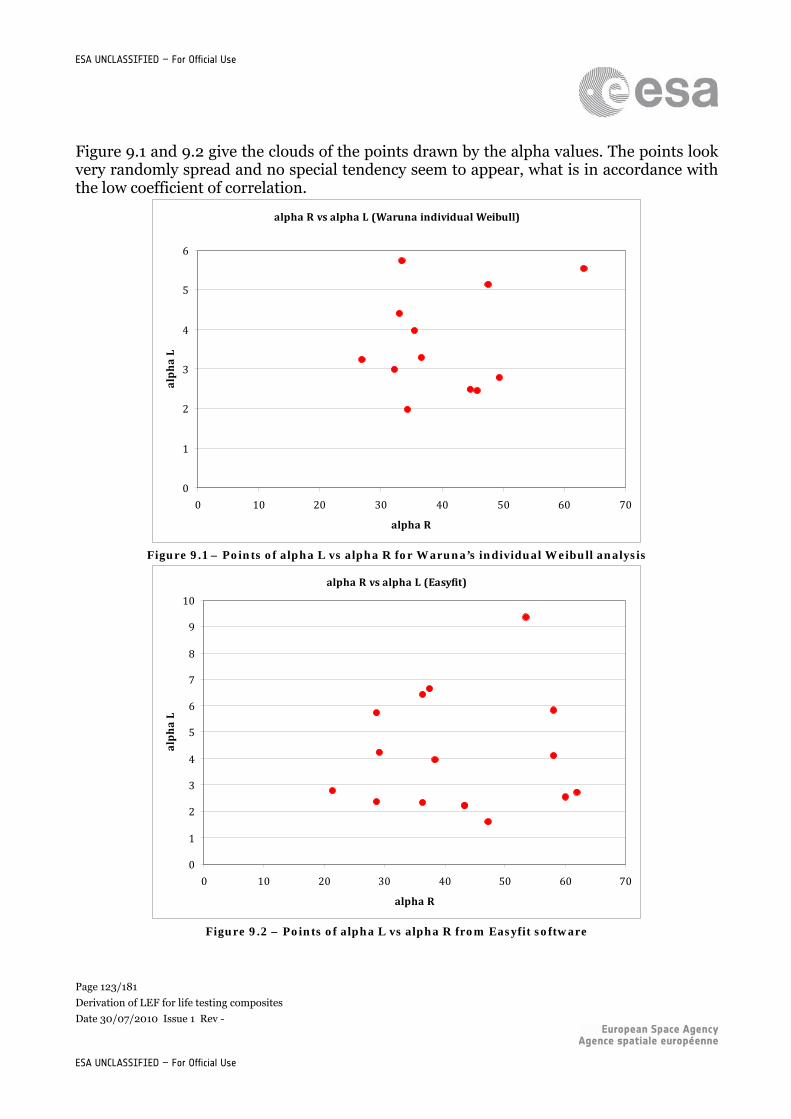
Page 123/181





Figure 9.1 and 9.2 give the clouds of the points drawn by the alpha values. The points look very randomly spread and no special tendency seem to appear, what is in accordance with the low coefficient of correlation.

alpha R vs alpha L (Waruna individual Weibull)

0

1

2

3

4

5

6

0 10 20 30 40 50 60 70

alpha R

alpha L

Figure 9.1 – Points of alpha L vs alpha R for Waruna’s individual Weibull analysis

alpha R vs alpha L (Easyfit)

0

1

2

3

4

5

6

7

8

9

10

0 10 20 30 40 50 60 70

alpha R

alpha L

Figure 9.2 – Points of alpha L vs alpha R from Easyfit software

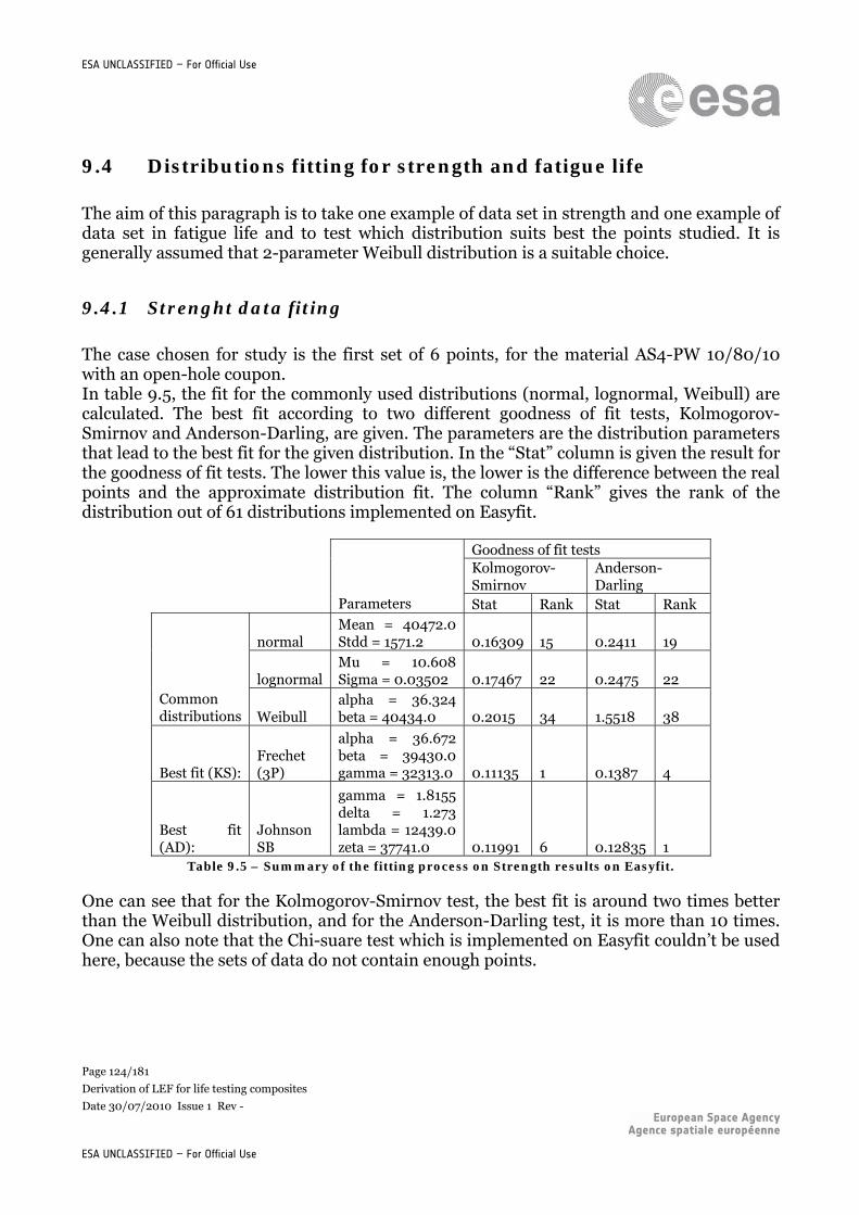
Page 124/181





9.4 Distributions fitting for strength and fatigue life

The aim of this paragraph is to take one example of data set in strength and one example of data set in fatigue life and to test which distribution suits best the points studied. It is generally assumed that 2-parameter Weibull distribution is a suitable choice.

9.4.1 Strenght data fiting

The case chosen for study is the first set of 6 points, for the material AS4-PW 10/80/10 with an open-hole coupon. In table 9.5, the fit for the commonly used distributions (normal, lognormal, Weibull) are calculated. The best fit according to two different goodness of fit tests, Kolmogorov-Smirnov and Anderson-Darling, are given. The parameters are the distribution parameters that lead to the best fit for the given distribution. In the “Stat” column is given the result for the goodness of fit tests. The lower this value is, the lower is the difference between the real points and the approximate distribution fit. The column “Rank” gives the rank of the distribution out of 61 distributions implemented on Easyfit.

Goodness of fit tests

Kolmogorov-Smirnov

Anderson-Darling

Parameters Stat Rank Stat Rank

normal Mean = 40472.0 Stdd = 1571.2 0.16309 15 0.2411 19

lognormal Mu = 10.608 Sigma = 0.03502 0.17467 22 0.2475 22

Common distributions Weibull

alpha = 36.324 beta = 40434.0 0.2015 34 1.5518 38

Best fit (KS): Frechet (3P)

alpha = 36.672 beta = 39430.0 gamma = 32313.0 0.11135 1 0.1387 4

Best fit (AD):

Johnson SB

gamma = 1.8155 delta = 1.273 lambda = 12439.0 zeta = 37741.0 0.11991 6 0.12835 1

Table 9.5 – Summary of the fitting process on Strength results on Easyfit.

One can see that for the Kolmogorov-Smirnov test, the best fit is around two times better than the Weibull distribution, and for the Anderson-Darling test, it is more than 10 times. One can also note that the Chi-suare test which is implemented on Easyfit couldn’t be used here, because the sets of data do not contain enough points.

Page 125/181





Figures 9.3, 9.4 and 9.5 show respectively the PDF, CDF and Survival functions, for the real set of data and for the fitting curves. Easyfit do not plot the data as points, but only gives them as histograms. On the PDF plot, one can see two green curves. The Frechet distribution is the one more on the left and the Weibull distribution is the one more on the right.

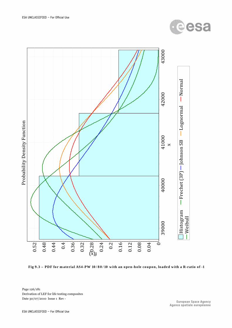
Page 126/181





Fig 9.3 – PDF for material AS4-PW 10/80/10 with an open-hole coupon, loaded with a R-ratio of -1

Probability Density Function

Histogram

Frechet (3P)

Johnson SB

Lognormal

Normal

Weibull

x43000

42000

41000

40000

39000

f(x)0.52

0.48

0.44 0.4

0.36

0.32

0.28

0.24 0.2

0.16

0.12

0.08

0.04 0

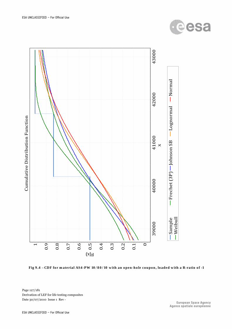
Page 127/181





Fig 9.4 –CDF for material AS4-PW 10/80/10 with an open-hole coupon, loaded with a R-ratio of -1

Cumulative Distribution Function

Sam

ple

Frechet (3P)

Johnson SB

Lognorm

al

Norm

al

Weibull

x43000

42000

41000

40000

39000

F(x)

1

0.9

0.8

0.7

0.6

0.5

0.4

0.3

0.2

0.1 0

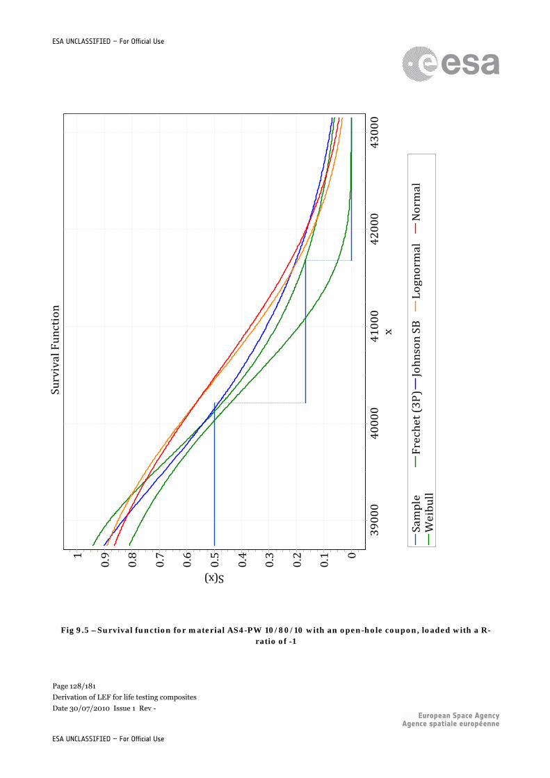
Page 128/181





Fig 9.5 –Survival function for material AS4-PW 10/80/10 with an open-hole coupon, loaded with a R-ratio of -1

Survival Function

Sample

Frechet (3P)

Johnson SB

Lognormal

Normal

Weibull

x43000

42000

41000

40000

39000

S(x)

1

0.9

0.8

0.7

0.6

0.5

0.4

0.3

0.2

0.1 0

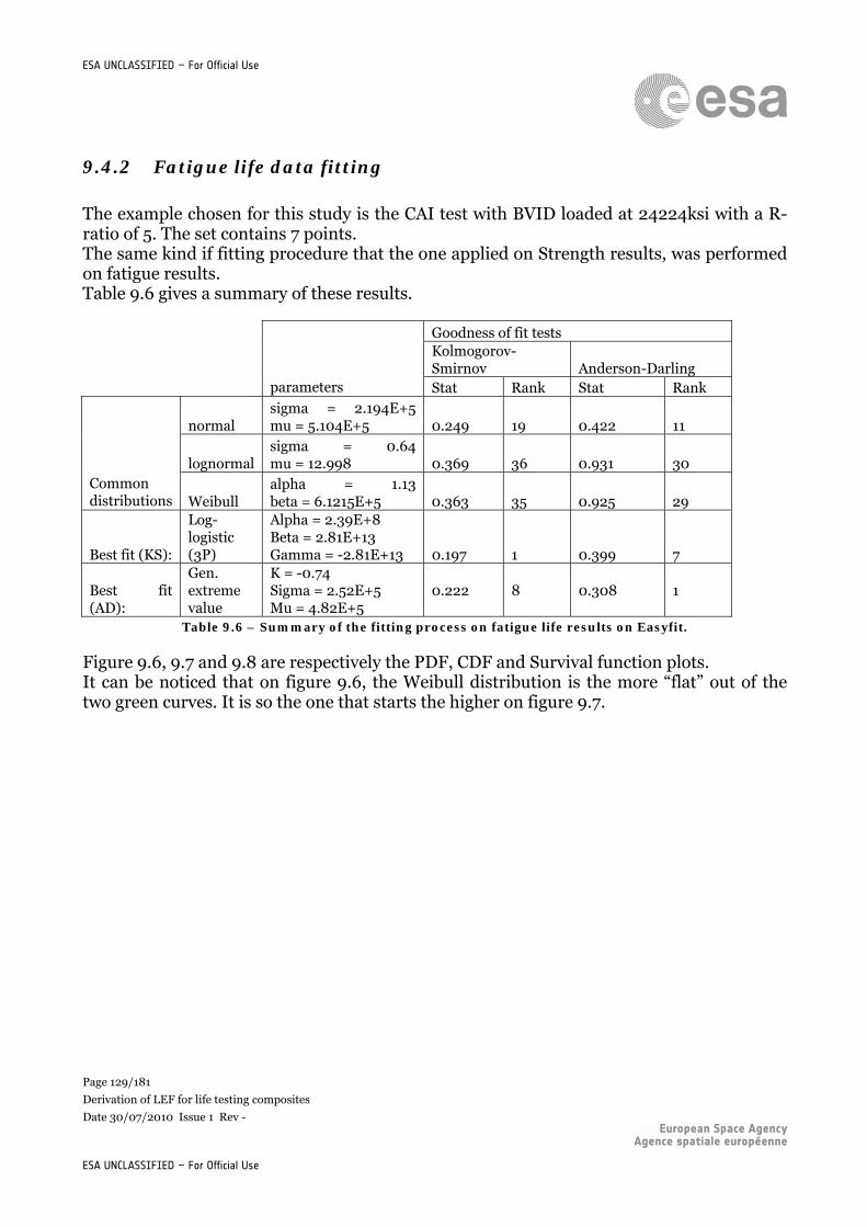
Page 129/181





9.4.2 Fatigue life data fitting

The example chosen for this study is the CAI test with BVID loaded at 24224ksi with a R-ratio of 5. The set contains 7 points. The same kind if fitting procedure that the one applied on Strength results, was performed on fatigue results. Table 9.6 gives a summary of these results.


Kolmogorov-Smirnov Anderson-Darling

parameters Stat Rank Stat Rank

normal sigma = 2.194E+5 mu = 5.104E+5 0.249 19 0.422 11

lognormal sigma = 0.64 mu = 12.998 0.369 36 0.931 30


alpha = 1.13 beta = 6.1215E+5 0.363 35 0.925 29

Best fit (KS):

Log-logistic (3P)

Alpha = 2.39E+8 Beta = 2.81E+13 Gamma = -2.81E+13 0.197 1 0.399 7

Best fit (AD):

Gen. extreme value

K = -0.74 Sigma = 2.52E+5 Mu = 4.82E+5

0.222 8 0.308 1

Table 9.6 – Summary of the fitting process on fatigue life results on Easyfit.

Figure 9.6, 9.7 and 9.8 are respectively the PDF, CDF and Survival function plots. It can be noticed that on figure 9.6, the Weibull distribution is the more “flat” out of the two green curves. It is so the one that starts the higher on figure 9.7.

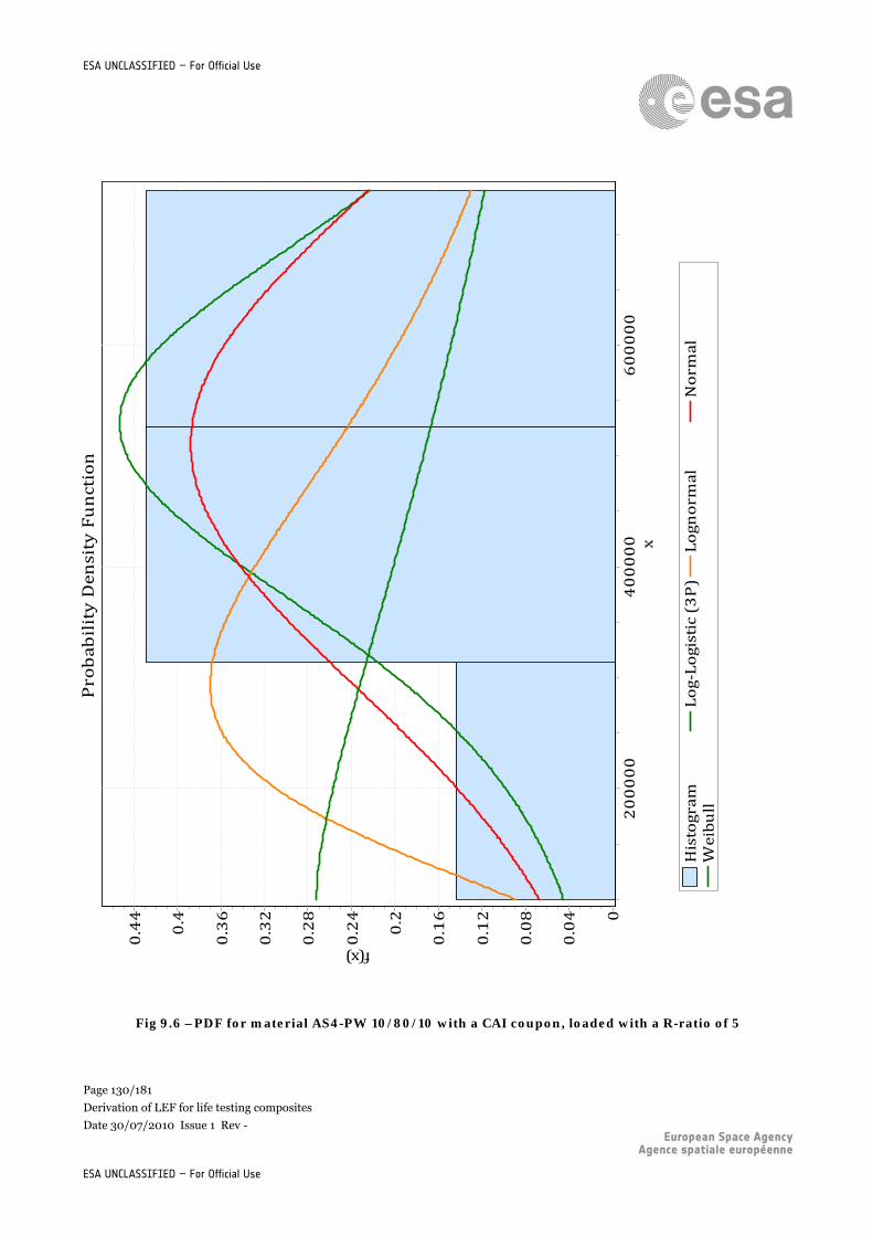
Page 130/181





Fig 9.6 –PDF for material AS4-PW 10/80/10 with a CAI coupon, loaded with a R-ratio of 5


Histogram

Log‐Logistic (3P)

Lognorm

alNorm

alWeibull

x600000

400000

200000

f(x)0.44

0.4

0.36

0.32

0.28

0.24

0.2

0.16

0.12

0.08

0.04 0

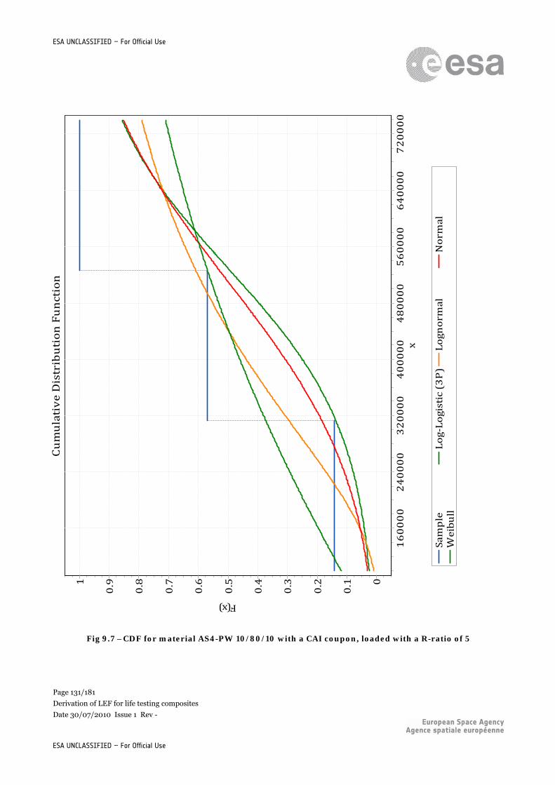
Page 131/181





Fig 9.7 –CDF for material AS4-PW 10/80/10 with a CAI coupon, loaded with a R-ratio of 5


Sample

Log‐Logistic (3P)

Lognorm

alNorm

alWeibull

x720000

640000

560000

480000

400000

320000

240000

160000

F(x)

1

0.9

0.8

0.7

0.6

0.5

0.4

0.3

0.2

0.1 0

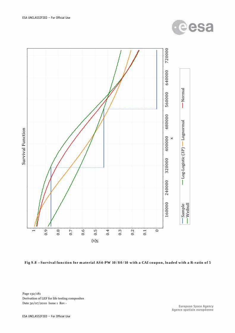
Page 132/181





Fig 9.8 –Survival function for material AS4-PW 10/80/10 with a CAI coupon, loaded with a R-ratio of 5

Survival Function

Sample

Log‐Logistic (3P)

Lognormal

Normal

Weibull

x720000

640000

560000

480000

400000

320000

240000

160000

S(x)

1

0.9

0.8

0.7

0.6

0.5

0.4

0.3

0.2

0.1 0

Page 133/181





9.5 Distributions fitting for alpha L and alpha R

This chapter is just for information, in case some reliability analysis had to be made, using alpha L and alpha R as stochastic variables, what means that alpha L and alpha R are the data points. The alpha values computed with Easyfit were used. The values are given in tables 9.1 and 9.3. 16 values of alpha R are available and 17 values of alpha L are given. Table 9.7 to 9.11 give the summary of the fitting analysis for the alpha R and alpha L values computed thanks to Easyfit. Then the figure 9.9 to 9.14 give PDF, CDF and survival functions of Alpha R and alpha R, for the most common distributions, since the ones that give usually the best fit are not implemented on FERUM (see chapter 8)

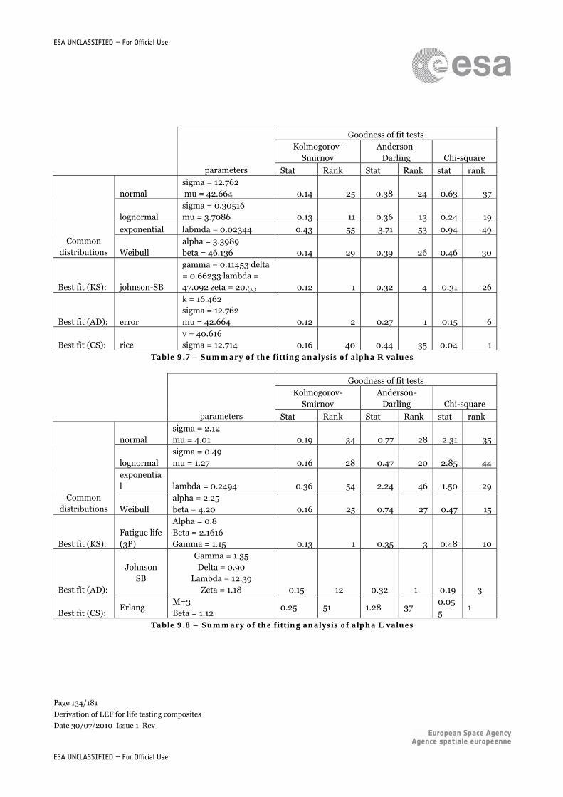
Page 134/181






Kolmogorov-

Smirnov Anderson-

Darling Chi-square

parameters Stat Rank Stat Rank stat rank

normal sigma = 12.762 mu = 42.664 0.14 25 0.38 24 0.63 37

lognormal sigma = 0.30516 mu = 3.7086 0.13 11 0.36 13 0.24 19

exponential labmda = 0.02344 0.43 55 3.71 53 0.94 49 Common

distributions Weibull alpha = 3.3989 beta = 46.136 0.14 29 0.39 26 0.46 30

Best fit (KS): johnson-SB

gamma = 0.11453 delta = 0.66233 lambda = 47.092 zeta = 20.55 0.12 1 0.32 4 0.31 26

Best fit (AD): error

k = 16.462 sigma = 12.762 mu = 42.664 0.12 2 0.27 1 0.15 6

Best fit (CS): rice v = 40.616 sigma = 12.714 0.16 40 0.44 35 0.04 1

Table 9.7 – Summary of the fitting analysis of alpha R values


Kolmogorov-

Smirnov Anderson-

Darling Chi-square

parameters Stat Rank Stat Rank stat rank

normal sigma = 2.12 mu = 4.01 0.19 34 0.77 28 2.31 35

lognormal sigma = 0.49 mu = 1.27 0.16 28 0.47 20 2.85 44

exponential lambda = 0.2494 0.36 54 2.24 46 1.50 29


alpha = 2.25 beta = 4.20 0.16 25 0.74 27 0.47 15

Best fit (KS): Fatigue life (3P)

Alpha = 0.8 Beta = 2.1616 Gamma = 1.15 0.13 1 0.35 3 0.48 10

Best fit (AD):

Johnson SB

Gamma = 1.35 Delta = 0.90

Lambda = 12.39 Zeta = 1.18 0.15 12 0.32 1 0.19 3

Best fit (CS): Erlang

M=3 Beta = 1.12

0.25 51 1.28 37 0.055

1

Table 9.8 – Summary of the fitting analysis of alpha L values

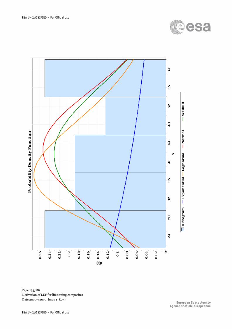
Page 135/181






Histogram

Exponential

Lognormal

Normal

Weibull

x60

56

52

48

44

40

36

32

28

24

f(x)

0.26

0.24

0.22

0.2

0.18

0.16

0.14

0.12

0.1

0.08

0.06

0.04

0.02 0

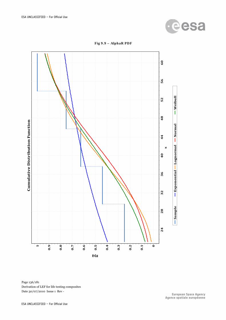
Page 136/181





Fig 9.9 – AlphaR PDF


Sample

Exponential

Lognormal

Normal

Weibull

x60

56

52

48

44

40

36

32

28

24

F(x)

1

0.9

0.8

0.7

0.6

0.5

0.4

0.3

0.2

0.1 0

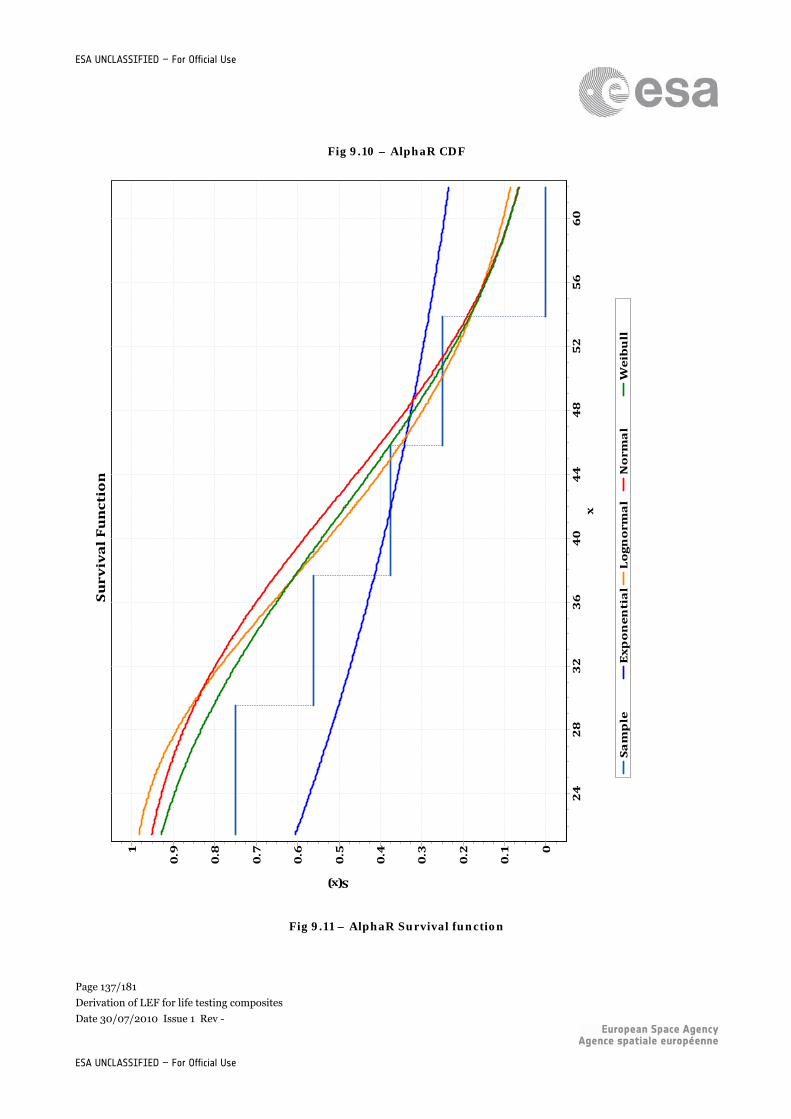
Page 137/181





Fig 9.10 – AlphaR CDF

Fig 9.11 – AlphaR Survival function

Survival Function

Sample

Exponential

Lognormal

Normal

Weibull

x60

56

52

48

44

40

36

32

28

24

S(x)

1

0.9

0.8

0.7

0.6

0.5

0.4

0.3

0.2

0.1 0

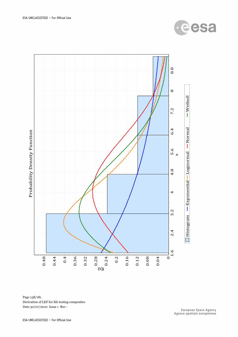
Page 138/181






Histogram

Exponential

Lognorm

al

Norm

al

Weibull

x8.8

87.2

6.4

5.6

4.8

43.2

2.4

1.6

f(x)0.48

0.44

0.4

0.36

0.32

0.28

0.24

0.2

0.16

0.12

0.08

0.04 0

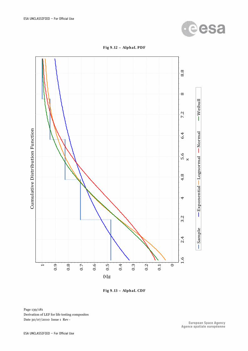
Page 139/181





Fig 9.12 – AlphaL PDF

Fig 9.13 – AlphaL CDF


Sample

Exponential

Lognorm

alNorm

alWeibull

x8.8

87.2

6.4

5.6

4.8

43.2

2.4

1.6

F(x)

1

0.9

0.8

0.7

0.6

0.5

0.4

0.3

0.2

0.1 0

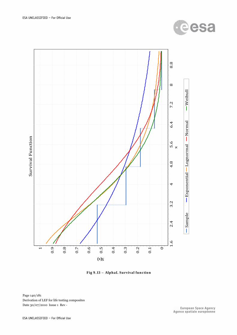
Page 140/181





Fig 9.13 – AlphaL Survival function

Survival Function

Sam

ple

Exponential

Lognorm

al

Norm

al

Weibull

x8.8

87.2

6.4

5.6

4.8

43.2

2.4

1.6

S(x)

1

0.9

0.8

0.7

0.6

0.5

0.4

0.3

0.2

0.1 0

Page 141/181





9.6 Conclusions

First, it seems important to notice that we are able to compute the Weibull scale and shape values of a given set of data. So we can reproduce Waruna’s methodology. But we didn’t always find the same results as he did. This might be explained by the fact that the solver used to solve the non linear equation giving alpha and beta values is probably not the same in the software used by Waruna and on Easyfit. This chapter has also be the occasion to evaluate the software Easyfit.. The interface is and easy to understand, but then the user is quickly limited, for instance we cannot control the bins size for the plot of histograms, the data can only be represented as histograms and not as points. And then, as seen before, some solvers might be more accurate, such as for instance the one used bu Waruna Severinate. Looking for another solver might be of interest, for example, a Statistical toolbox exists for matlab, that gives the fit of the most common distributions. But this kind of additional toolbox cost a lot, and it is not sure that it is worth buying such tools just for our analysis. Then we can also assess that 6 points per batch does not appear to be enough to obtain some accurate estimates It was assumed in the 80’s that the Weibull distribution was the best distribution to fit fatigue and strength data. But from all the fitting analysis performed during this study, the Weibull distribution never was the best fit according to the 2 goodness of fit tests. And in many cases, the normal or the lognormal distributions fitted better than the Weibull distribution.

Page 142/181





10 OTHER TOOLS FOR FULL SCALE TESTING

10.1 The use of safety and proof factors for full scale testing

All the informations contained in this chapter are taken from the standars requirements if NASA, ISS and ESA (ref[29] to ref[33]). Safety and proof factors are multiplicative factors that increase parameters that influence the strength or life of a structure (loads, environmental conditions…) during tests or for design. The purpose of the use of these factors is to guarantee a certain level of mechanical reliability. They can be applied to satellites, payloads, launch vehicle structural elements, equipments, experiments, and their value depend on the level of reliability required, the complexity of the structure and whether the structure is used for a manned mission or not.

10.1.1 Safety factors

Safety factors are multiplying factors to be applied to limit loads or stresses for purposes of analytical assessment (design factors) or test verification (test factors) of design adequacy in strength or stability. Some important typical load values that need to be tested and increased during test are ultimate and yield load. They both have their own factor safety, FOSU (ultimate design factor of safety) and FOSY (yield design factor of safety), which are multiplying factors applied to the design limit load to get respectively the design ultimate load, and the design yield load. While MIL-HDBK 17 vol 3 requires a FOSU value of 1.5 for aircraft structures, international space station program, NASA and ESA require different values according to the use of the space structure.

10.1.2 Proof test

A proof test is a test performed on the flight hardware to verify workmanship, material quality, and structural integrity of the item. In the protoflight structural verification approach, proof, acceptance, and protoflight tests are synonymous. During that test, the load applied is the proof load, which is the limit load multiplicated by a factor called proof test factor. A difference has to be done between protoflight and prototype tests. As already explained, protoflight tests are performed on the flight hardware, whereas prototype tests are performed on a separate flight-like structural test article to verify structural integrity of the design. A synonym of prototype test is qualification test.

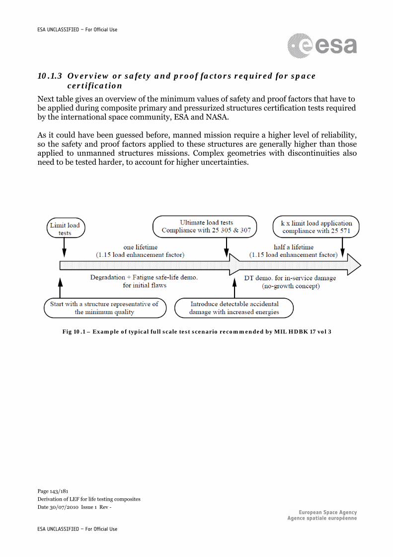
Page 143/181





10.1.3 Overview or safety and proof factors required for space certification

Next table gives an overview of the minimum values of safety and proof factors that have to be applied during composite primary and pressurized structures certification tests required by the international space community, ESA and NASA. As it could have been guessed before, manned mission require a higher level of reliability, so the safety and proof factors applied to these structures are generally higher than those applied to unmanned structures missions. Complex geometries with discontinuities also need to be tested harder, to account for higher uncertainties.

Fig 10.1 – Example of typical full scale test scenario recommended by MIL HDBK 17 vol 3

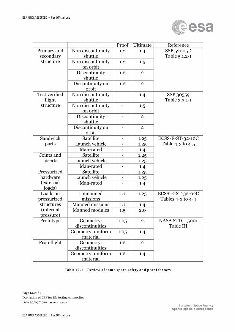
Page 144/181





Proof Ultimate Reference Non discontinuity

shuttle 1.2 1.4

Non discontinuity on orbit

1.2 1.5

Discontinuity shuttle

1.2 2

Primary and secondary structure

Discontinuity on orbit

1.2 2

SSP 52005D Table 5.1.2-1

Non discontinuity shuttle

- 1.4

Non discontinuity on orbit

- 1.5

Discontinuity shuttle

- 2

Test verified flight

structure

Discontinuity on orbit

- 2

SSP 30559 Table 3.3.1-1

Satellite - 1.25 Launch vehicle - 1.25

Sandwich parts

Man-rated - 1.4 Satellite - 1.25

Launch vehicle - 1.25 Joints and

inserts Man-rated - 1.4

Satellite - 1.25 Launch vehicle - 1.25

Pressurized hardware (external

loads) Man-rated - 1.4

ECSS-E-ST-32-10C Table 4-3 to 4-5

Unmanned missions

1.1 1.25

Manned missions 1.1 1.4

Loads on pressurized structures (internal pressure)

Manned modules 1.5 2.0

ECSS-E-ST-32-02C Tables 4-2 to 4-4

Geometry: discontinuities

1.05 2 Prototype

Geometry: uniform material

1.05 1.4

Geometry: discontinuities

1.2 2 Protoflight

Geometry: uniform material

1.2 1.4

NASA STD – 5001 Table III

Table 10.1 – Review of some space safety and proof factors

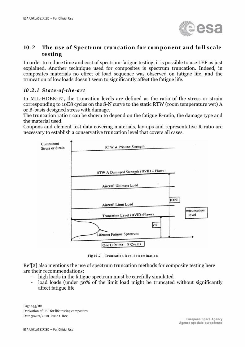
Page 145/181





10.2 The use of Spectrum truncation for component and full scale testing

In order to reduce time and cost of spectrum-fatigue testing, it is possible to use LEF as just explained. Another technique used for composites is spectrum truncation. Indeed, in composites materials no effect of load sequence was observed on fatigue life, and the truncation of low loads doesn’t seem to significantly affect the fatigue life.

10.2.1 State-of-the-art

In MIL-HDBK-17 , the truncation levels are defined as the ratio of the stress or strain corresponding to 10E8 cycles on the S-N curve to the static RTW (room temperature wet) A or B-basis designed stress with damage. The truncation ratio r can be shown to depend on the fatigue R-ratio, the damage type and the material used. Coupons and element test data covering materials, lay-ups and representative R-ratio are necessary to establish a conservative truncation level that covers all cases.

Fig 10.2 – Truncation level determination

Ref[2] also mentions the use of spectrum truncation methods for composite testing here are their recommendations:

- high loads in the fatigue spectrum must be carefully simulated - load loads (under 30% of the limit load might be truncated without significantly

affect fatigue life

Page 146/181





- this method should not be used for mixed metal/composites structures. - Anyway, LEF use is recommended.

In ref[21], an overview of the spectrum truncation methods used in industry is made:

- raytheon “star ship”: Truncation level of 10E7 cycles for static components and 10E8 cycles for rotating high cycles components based on static coupons test data.

- Sikorsky helicopter: Blade certification generic approach: truncation level at 10E8 cycle equivalent strain adjusted for conditioned strength based on static coupon test data

- Boeing 737 & 777: Choice of truncation levels was based on the general transport aircraft industry approach that truncates loads such that only 100 applied cycles per flight are treated as damaging.

- Commercial Boeing 777 empennage torque box: Demonstrated no growth of damage at the threshold of detectability under repeated loading for a minimum of two livetimes. Residual strength for several damage scenarios is demonstrated after application of the repeated loading

10.2.2 Results of J.SCHÖN spectrum truncation testing

J.Schön defines the truncation levels as the threshold percentage of the overall peak-to-peak load range of the spectra under which load cycles are truncated.

10.2.2.1 Tests achieved with the vertical tail fighter aircraft spectrum: the bfkb spectrum

10.2.2.1.1 Spectrum description The bfkb spectrum is nearly symmetric and is from the vertical tail of a fighter aircraft, the JAS39 Gripen. The number of cycles in the spectrum was reduced was reduced by eliminating low amplitude cycles.

- bfkb: basic fighter aircraft spectrum, which contains 8670 cycles. - bvkb30: ovkb spectrum truncated from all load cycles with a load range less than

30% of the overall peak-to-peak load range of the spectra, it contains 1821 cycles - bvbk50: ovbk with 50% elimination, it contains 808 cycles.

These three spectra are plotted in fig 10.3, where the number of cycles plotted at a load level is the total number of load values counted from the maximum peak or though value

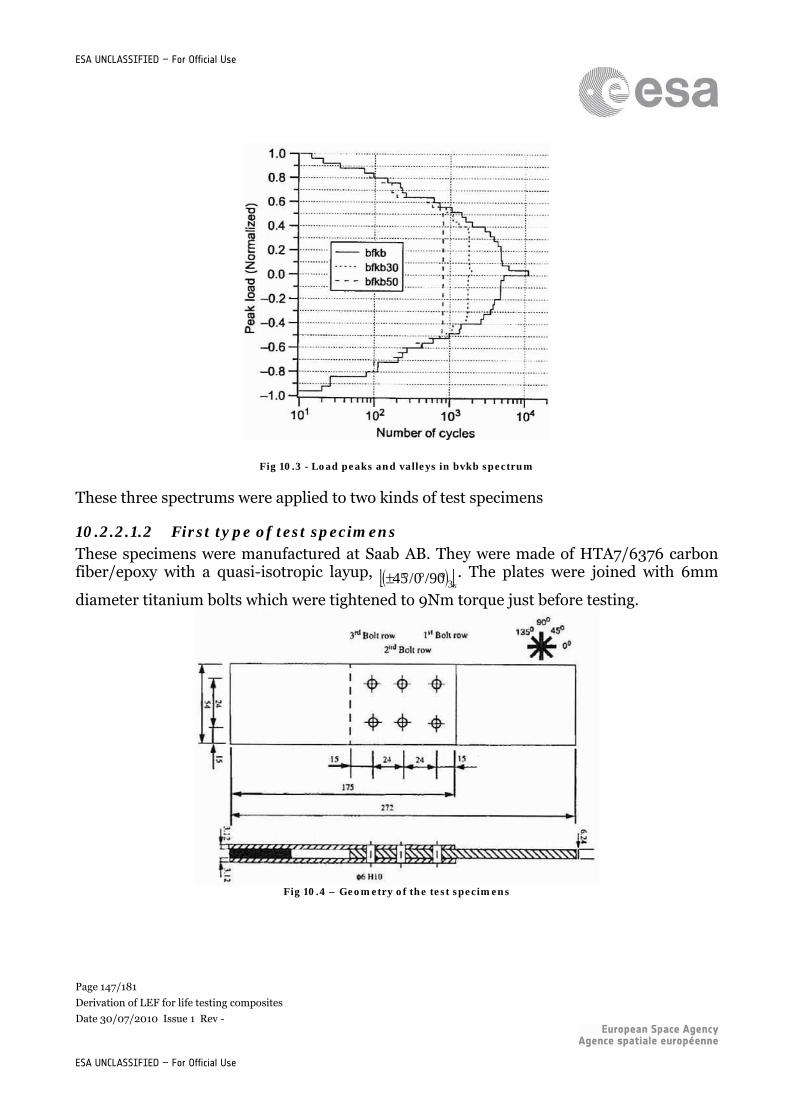
Page 147/181





Fig 10.3 - Load peaks and valleys in bvkb spectrum

These three spectrums were applied to two kinds of test specimens

10.2.2.1.2 First type of test specimens These specimens were manufactured at Saab AB. They were made of HTA7/6376 carbon fiber/epoxy with a quasi-isotropic layup, 90/0/45 3S

. The plates were joined with 6mm

diameter titanium bolts which were tightened to 9Nm torque just before testing.

Fig 10.4 – Geometry of the test specimens

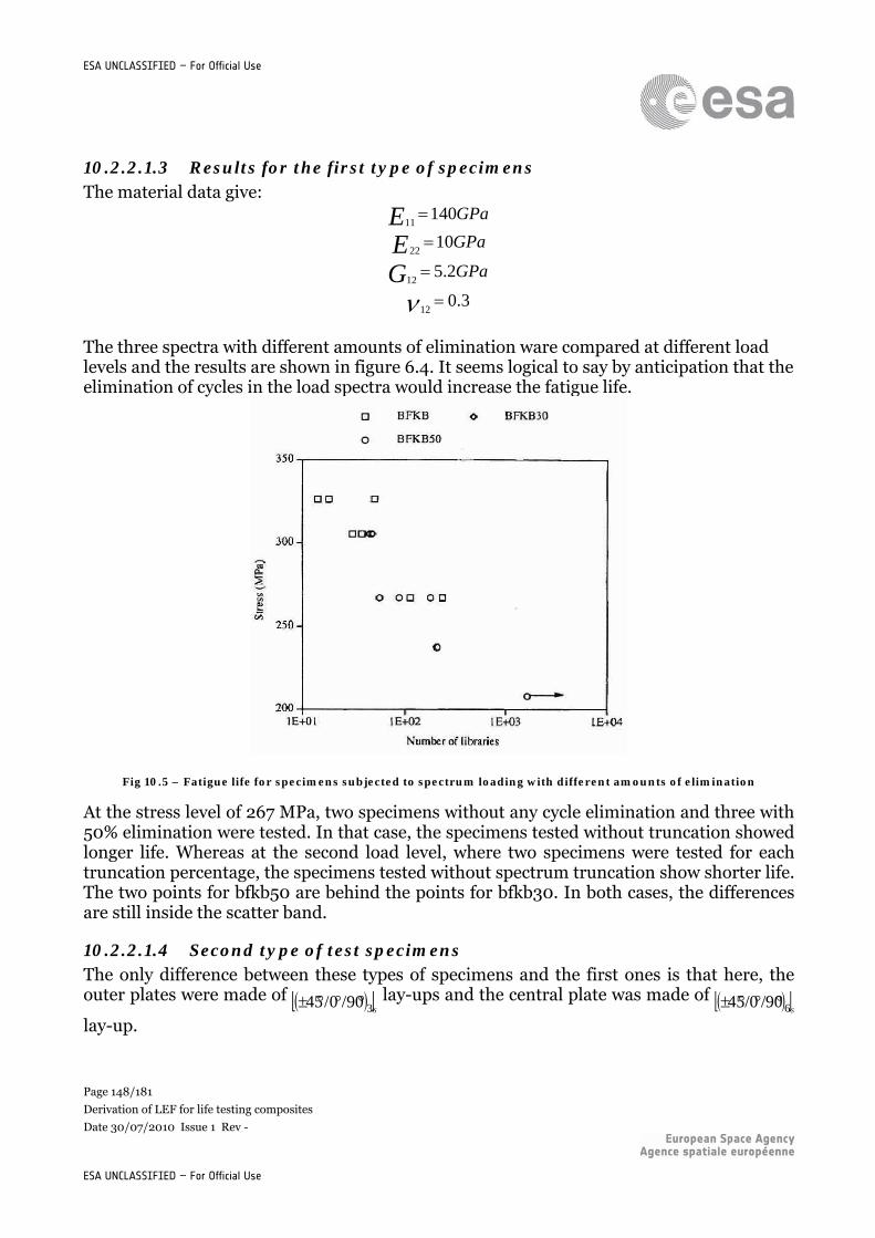
Page 148/181





10.2.2.1.3 Results for the first type of specimens The material data give:

GPaE 14011

GPaE 1022

GPaG 2.512

3.012

The three spectra with different amounts of elimination ware compared at different load levels and the results are shown in figure 6.4. It seems logical to say by anticipation that the elimination of cycles in the load spectra would increase the fatigue life.

Fig 10.5 – Fatigue life for specimens subjected to spectrum loading with different amounts of elimination

At the stress level of 267 MPa, two specimens without any cycle elimination and three with 50% elimination were tested. In that case, the specimens tested without truncation showed longer life. Whereas at the second load level, where two specimens were tested for each truncation percentage, the specimens tested without spectrum truncation show shorter life. The two points for bfkb50 are behind the points for bfkb30. In both cases, the differences are still inside the scatter band.

10.2.2.1.4 Second type of test specimens The only difference between these types of specimens and the first ones is that here, the outer plates were made of 90/0/45 3S

lay-ups and the central plate was made of 90/0/45 6S

lay-up.

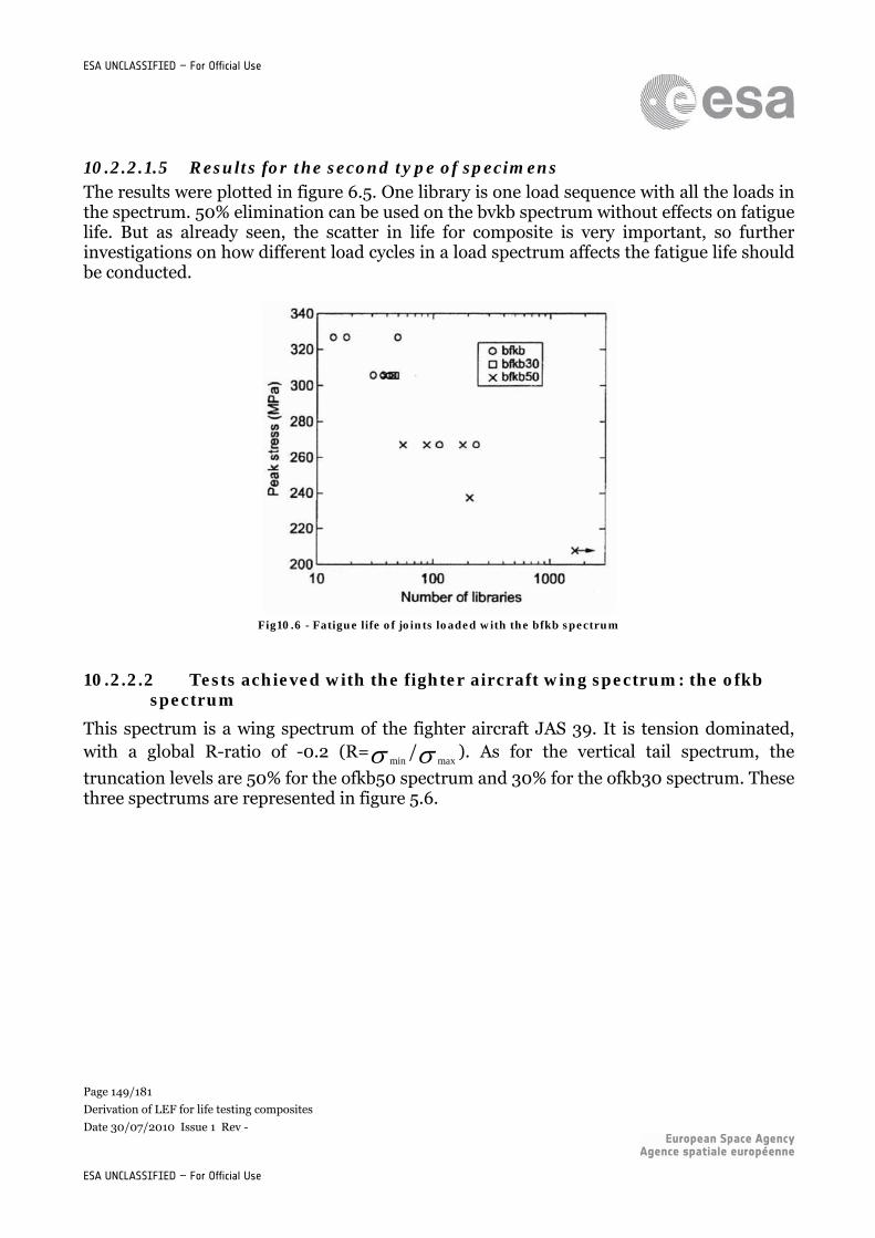
Page 149/181





10.2.2.1.5 Results for the second type of specimens The results were plotted in figure 6.5. One library is one load sequence with all the loads in the spectrum. 50% elimination can be used on the bvkb spectrum without effects on fatigue life. But as already seen, the scatter in life for composite is very important, so further investigations on how different load cycles in a load spectrum affects the fatigue life should be conducted.

Fig10.6 - Fatigue life of joints loaded with the bfkb spectrum

10.2.2.2 Tests achieved with the fighter aircraft wing spectrum: the ofkb spectrum

This spectrum is a wing spectrum of the fighter aircraft JAS 39. It is tension dominated, with a global R-ratio of -0.2 (R= min

/ max). As for the vertical tail spectrum, the

truncation levels are 50% for the ofkb50 spectrum and 30% for the ofkb30 spectrum. These three spectrums are represented in figure 5.6.

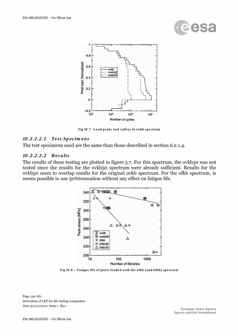
Page 150/181





Fig 10.7 - Load peaks and valleys in ovkb spectrum

10.2.2.2.1 Test Specimens The test specimens used are the same than those described in section 6.2.1.4.

10.2.2.2.2 Results The results of these testing are plotted in figure 5.7. For this spectrum, the ovkb30 was not tested since the results for the ovkb50 spectrum were already sufficient. Results for the ovkb50 seem to overlap results for the original ovkb spectrum. For the ofkb spectrum, is seems possible to use 50%truncation without any effect on fatigue life.

Fig 10.8 – Fatigue life of joints loaded with the ofkb (and bfkb) spectrum

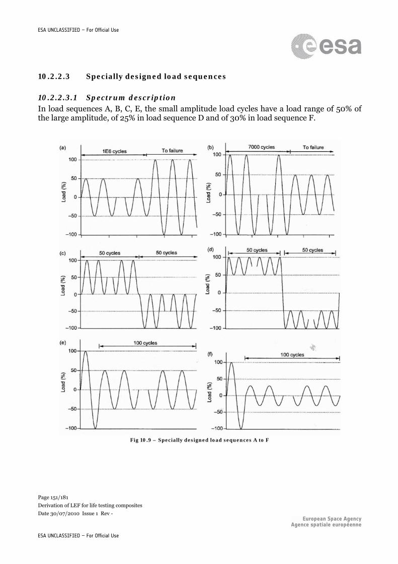
Page 151/181





10.2.2.3 Specially designed load sequences

10.2.2.3.1 Spectrum description In load sequences A, B, C, E, the small amplitude load cycles have a load range of 50% of the large amplitude, of 25% in load sequence D and of 30% in load sequence F.

Fig 10.9 – Specially designed load sequences A to F

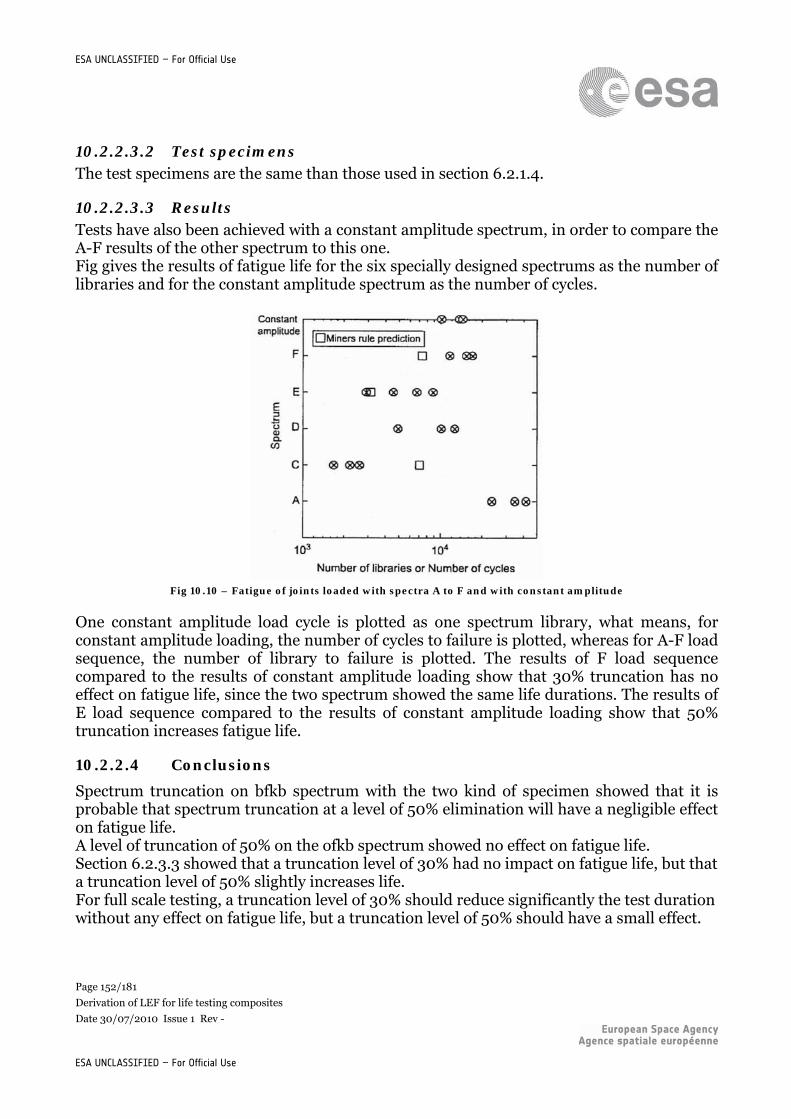
Page 152/181





10.2.2.3.2 Test specimens The test specimens are the same than those used in section 6.2.1.4.

10.2.2.3.3 Results Tests have also been achieved with a constant amplitude spectrum, in order to compare the A-F results of the other spectrum to this one. Fig gives the results of fatigue life for the six specially designed spectrums as the number of libraries and for the constant amplitude spectrum as the number of cycles.

Fig 10.10 – Fatigue of joints loaded with spectra A to F and with constant amplitude

One constant amplitude load cycle is plotted as one spectrum library, what means, for constant amplitude loading, the number of cycles to failure is plotted, whereas for A-F load sequence, the number of library to failure is plotted. The results of F load sequence compared to the results of constant amplitude loading show that 30% truncation has no effect on fatigue life, since the two spectrum showed the same life durations. The results of E load sequence compared to the results of constant amplitude loading show that 50% truncation increases fatigue life.

10.2.2.4 Conclusions

Spectrum truncation on bfkb spectrum with the two kind of specimen showed that it is probable that spectrum truncation at a level of 50% elimination will have a negligible effect on fatigue life. A level of truncation of 50% on the ofkb spectrum showed no effect on fatigue life. Section 6.2.3.3 showed that a truncation level of 30% had no impact on fatigue life, but that a truncation level of 50% slightly increases life. For full scale testing, a truncation level of 30% should reduce significantly the test duration without any effect on fatigue life, but a truncation level of 50% should have a small effect.

Page 153/181





CONCLUSIONS

The assumptions, underlying LEF derivations were explored and understood.

About the testing program issue, standard test methods on coupons exist (except for impact damage), and LEF test matrices have been found, but for airplane structures. The definition of specimen test program for space applications is open, and some questions still have to be answered: which tests shall be made on coupons, subcomponents and components? Is six specimens per batch enough? If so, how many shall be tested then?

3 data scatter analysis methods have been studied. The Joint Weibull method

appears to be the most appropriate and the most commonly used.

No clear conclusion can be made about the influence of impact damage on scatter in life and in strength, compared to the scatter observed for undamaged material.

The LEF model appears to be more sensitive to the strength shape parameter than

to its other parameters (fatigue shape parameter and test duration).

All LEF values found in literature are below 1.20, for aircraft applications

The influence of Weibull scale parameter beta (which is not considered in the derivation of the LEF) has to be studied, since it also influences the scatter.

Shape parameter values below 1 would mean premature failures. In some cases such

values below 1 are reported (resulting in relatively high LEF), but it is not clear in how far it is realistic to take into account such values for LEF derivation. It would be interesting to investigate in more detail how good the underlying data are described by the Weibull distribution, and whether the goodness of the fit is significantly affected by the choice of higher alpha with corresponding beta. Insufficient detailed data are currently available to perform this assessment.

The results of this study have possible implications for an update of ECSS-E-ST-32-

01, but some questions are not answered yet: shall shape parameters values be computed for every new design? shall a new default LEF value and new test duration be selected? And which values? (e.g. LEF=1.1 for N=4?)

The results of distribution fitting in chapter 9 indicate that some distributions which

are easier to use than the Weibull distribution fit better the investigated data points. It may therefore be interesting to investigate whether an alternative LEF derivation

Page 154/181





based on these distributions may be possible (for which distribution) and advantageous.

An effective damage tolerance verification of composite space structures consists not

only of LEF definition, but should also employ efficiently spectrum truncation, applied design safety factors and static qualification test and proof test factors. In order to limit the risks associated with increased load levels due to the LEF (e.g. change of failure mode, fatigue regime, …) it may also be considered to use the life factor (Nf) instead of LEF for the highest loads in the spectrum, for which the number of cycles is limited. In that case, also a default Nf may have to be defined. Furthermore some open questions remain on how to use effectively the specimen results in terms of lifetime (‘beta’) and not just scatter (‘alpha’).

Page 155/181





REFERENCES: [1] MIL-HDBK 17F, Volume 3, 2002 [2] Certification Testing Methodology for Composite Structure Vol I. and II. R.S. Whitehead, Oktober 1986 [3] The use of load enhancement factors in the certification of composite aircraft structures, J. Lameris, NLR, Netherlands. [4] Load enhancement factor to be applied on fatigue test for certification of composites, Jose Manuel Ruiz Barragen, EADS-CASA, Getafe, Spain [5] Design of high performance composite structures State-of-art and Challenge, Michele Thomas, AIRBUS, 2008 [6] Fatigue life determination of damage tolerant composite airframe, Waruna Prasanna Severinate, PhD report, December 2008 [7] Considerations for choosing a Default Value for the LEF, G.Faile, January 2010 [8] Advances Engineerin Mathematics, Erwin kreyszig, fourth edition. [9] Applied Statistics and Probability for Engineers, Douglas C. Montgomery and George C. Runger. [10] ASM HDBK of engineering mathematics [11] Handbook of mathematical functions, Abramowitz and Stegun [12] Fitting Model to Composite Materials Fatigue Data, G.P.Sendeckyj, Test Methods and Design Allowables for Fibrous Composites, ASTM STP 734 [13] ASM HDBK Vol 19 Fatigue and fracture [14] ASM HDBK Vol 21 Composites [15] Fatigue in composites, CRC, Brian Harris, 2003 [16] Composite materials: engineering and science, F.L. Matthews and R.D. Rawlings, 1995 [17] Computational approach for composite material allowable using sealed envelope predictions for reduced testing.

Page 156/181





[18] Fracture mechanics methods to assess mono and multi-delamination behaviour of aerospace composites, D. Guédra-Degeorges EADS France 2008 [19] 777 Empennage certification approach, A. Fawcet, J. Trostle, S. Ward, Boeing commercial Airplane Groupe, Seattle, Washiongton, USA, 1997 [20] Advanced certification methology for composite structures, Kan, H.P., Cordero, R., and Whitehead, R.S. April 1997 [21] Full scale testing of blades: now, and for the future, Josef Kryger Tadich and Jakob Wedel-Heinen, May 2007 [22] Spectrum fatigue of bolted joints, Joakim Schön and Tonny Nyman, Swedish Defense Research Agency, 2002 [23] Fatigue life prediction and load cycle elimination during spectrum loading of composites, Swedish Defense Research Agency, 2002 [24] Spectrum fatigue loading of composite bolted joints – small cycle elimination, Joakim Schön, Swedish Defense research Agency, 2005 [25] Damage tolerance in advanced composites – Sieranowski, Newas – technomic publishing company [26] LEF for composite test spectra (Raytheon method), Ric Abbott, Damage Tolerance Workshop, July 2006 [27] The effect of loading parameters on fatigue of composite laminates: part III, FAA report – Whitehead [28] Engineer_Statistics_Handbook [29] NASA-STD-5001 Structural Design and test factors of safety for spaceflight hardware June 21, 1996 [30] SSP 30559-international space station program-Structural Design and Verification Requirements [31] SSP 52005D-International space station program-Payload Flight Equipment Requirements and Guidelines for Safety-Critical Structures

Page 157/181





[32] ECSS-E-ST-32-02C Rev. 1-Structural design and verification of pressurized hardware 15 November 2008 [33] ECSS-E-ST-32-10C Rev.1-Structural factors of safety for spaceflight hardware 6 March 2009

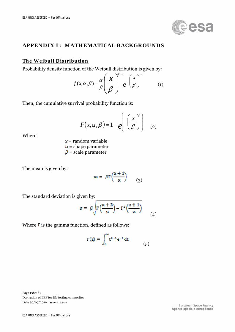
Page 158/181





APPENDIX I : MATHEMATICAL BACKGROUNDS

The Weibull Distribution

Probability density function of the Weibull distribution is given by:

ex x

xf

11

),,( (1)

Then, the cumulative survival probability function is:

ex

xF

1,, (2)

Where x = random variable = shape parameter = scale parameter The mean is given by:

(3)

The standard deviation is given by:

(4) Where is the gamma function, defined as follows:

(5)

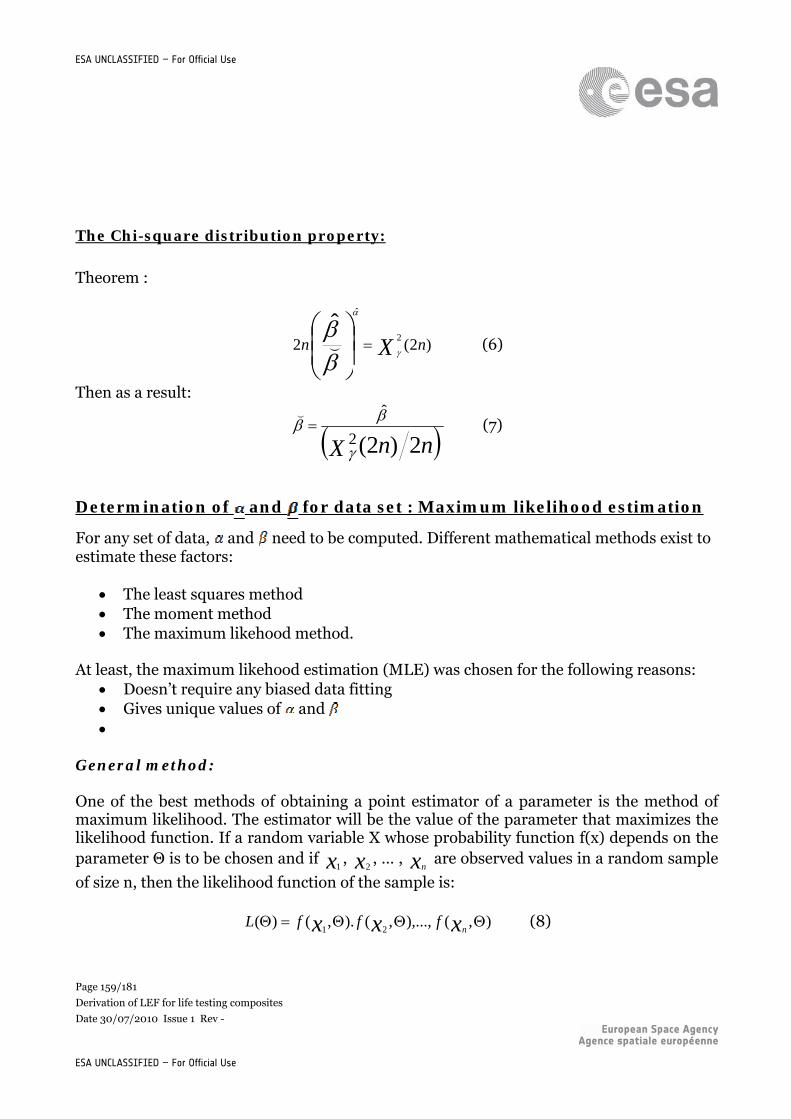
Page 159/181





The Chi-square distribution property:

Theorem :

)2(22

ˆ

ˆnn X

(6)

Then as a result:

nnX 2)2(2

ˆ

(7)

Determination of and for data set : Maximum likelihood estimation

For any set of data, and need to be computed. Different mathematical methods exist to estimate these factors:

The least squares method The moment method The maximum likehood method.

At least, the maximum likehood estimation (MLE) was chosen for the following reasons:

Doesn’t require any biased data fitting Gives unique values of and

General method: One of the best methods of obtaining a point estimator of a parameter is the method of maximum likelihood. The estimator will be the value of the parameter that maximizes the likelihood function. If a random variable X whose probability function f(x) depends on the parameter Θ is to be chosen and if x1

, x2, … , xn

are observed values in a random sample

of size n, then the likelihood function of the sample is:

),(),...,,().,()(21

xxx nfffL (8)

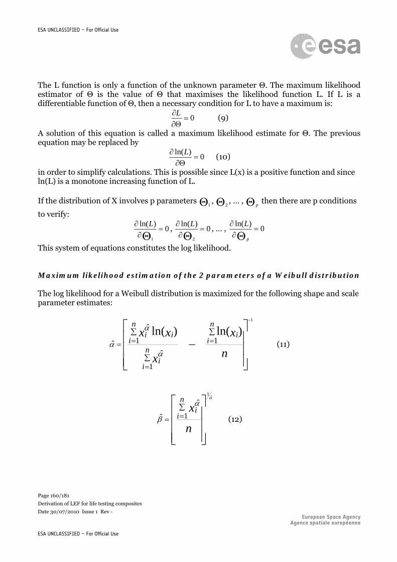
Page 160/181





The L function is only a function of the unknown parameter Θ. The maximum likelihood estimator of Θ is the value of Θ that maximises the likelihood function L. If L is a differentiable function of Θ, then a necessary condition for L to have a maximum is:

0L

(9)

A solution of this equation is called a maximum likelihood estimate for Θ. The previous equation may be replaced by

0)ln(

L

(10)

in order to simplify calculations. This is possible since L(x) is a positive function and since ln(L) is a monotone increasing function of L. If the distribution of X involves p parameters 1

, 2, … , p

then there are p conditions

to verify:

0)ln(

1

L

, 0)ln(

2

L

, … , 0)ln(

p

L

This system of equations constitutes the log likelihood. Maximum likelihood estimation of the 2 parameters of a Weibull distribution The log likelihood for a Weibull distribution is maximized for the following shape and scale parameter estimates:

n

x

x

xxn

ii

n

ii

n

iii

1

1

ˆ

1

ˆ

ˆ

)ln()ln(1

(11)

n

xn

ii

1

ˆ

ˆ

ˆ1

(12)

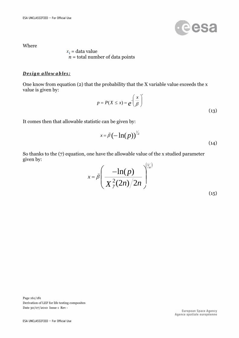
Page 161/181





Where = data value

n = total number of data points Design allowables: One know from equation (2) that the probability that the X variable value exceeds the x value is given by:

ex

xXPp

)(

(13) It comes then that allowable statistic can be given by:

))ln(( ˆ1

px

(14) So thanks to the (7) equation, one have the allowable value of the x studied parameter given by:

nnX

px

2)2(

)ln(2

1

(15)

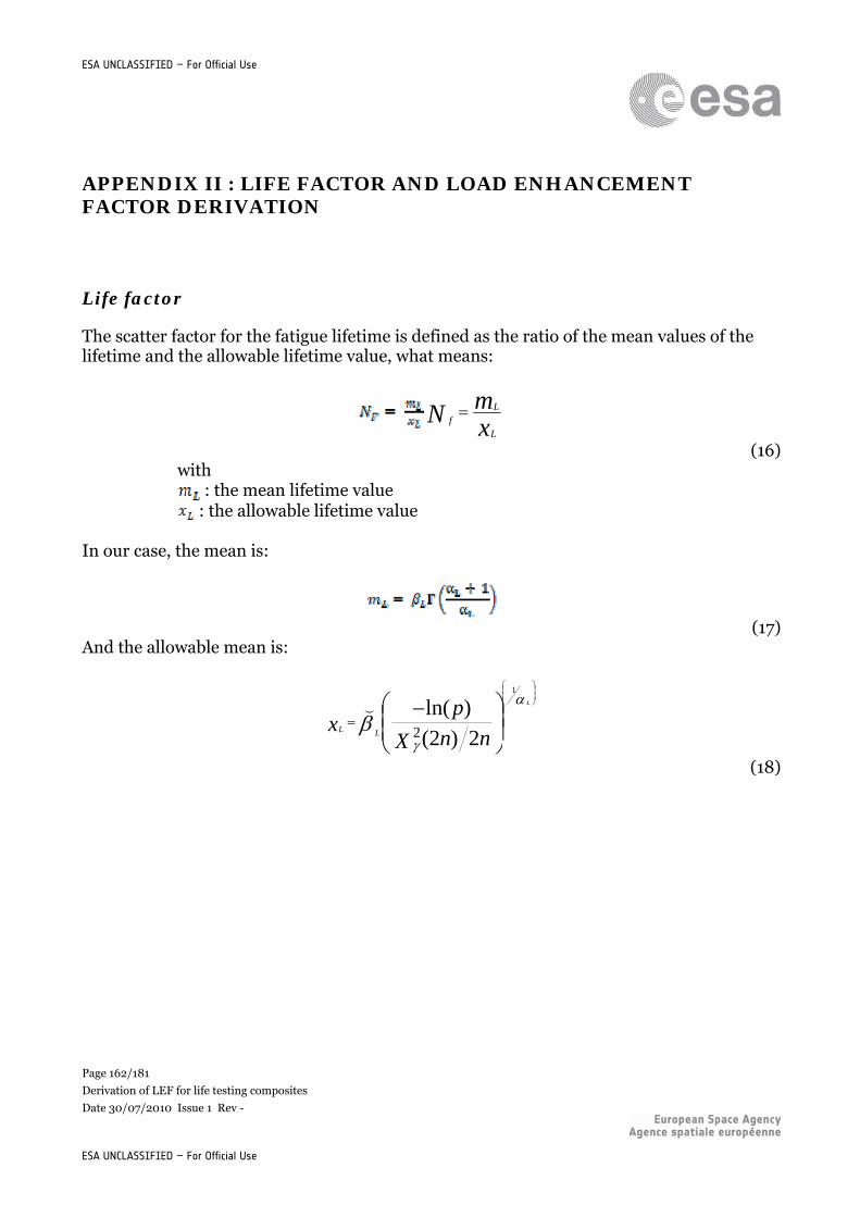
Page 162/181





APPENDIX II : LIFE FACTOR AND LOAD ENHANCEMENT FACTOR DERIVATION

Life factor

The scatter factor for the fatigue lifetime is defined as the ratio of the mean values of the lifetime and the allowable lifetime value, what means:

xmN

L

Lf

(16) with

: the mean lifetime value : the allowable lifetime value

In our case, the mean is:

(17)

And the allowable mean is:

nnX

px

L

LL

2)2(

)ln(2

1

(18)

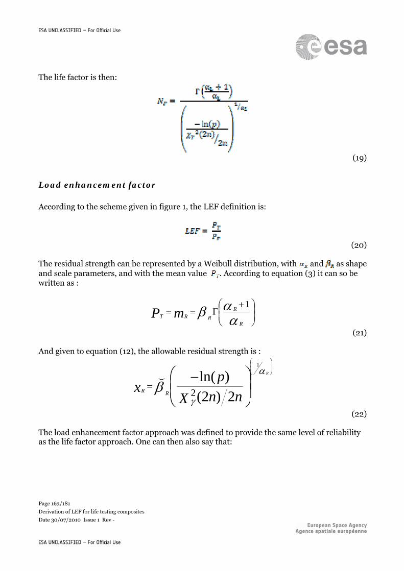
Page 163/181





The life factor is then:

(19)

Load enhancement factor

According to the scheme given in figure 1, the LEF definition is:

(20)

The residual strength can be represented by a Weibull distribution, with and as shape and scale parameters, and with the mean value . According to equation (3) it can so be written as :

R

R

RRT mP1

(21) And given to equation (12), the allowable residual strength is :

nnX

px

R

RR

2)2()ln(

2

1

(22) The load enhancement factor approach was defined to provide the same level of reliability as the life factor approach. One can then also say that:

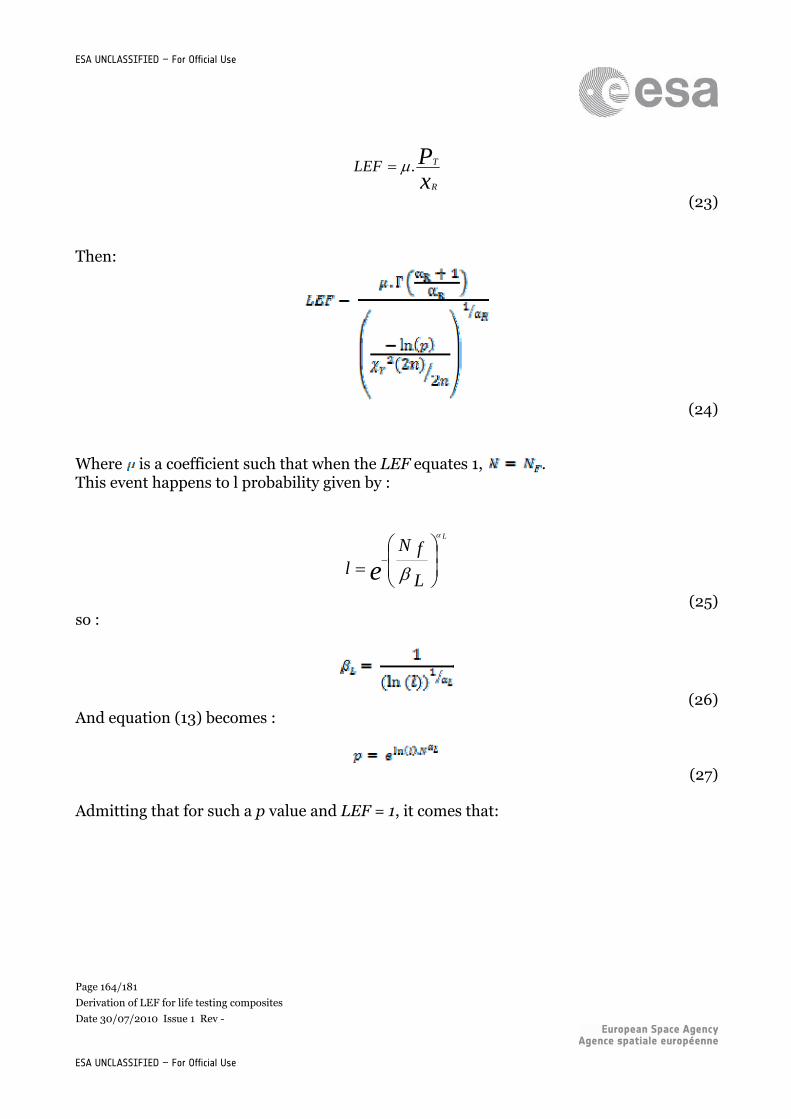
Page 164/181





xP

R

TLEF .

(23) Then:

(24)

Where is a coefficient such that when the LEF equates 1, . This event happens to l probability given by :

e L

N fl

L

(25) so :

(26)

And equation (13) becomes :

(27)

Admitting that for such a p value and LEF = 1, it comes that:

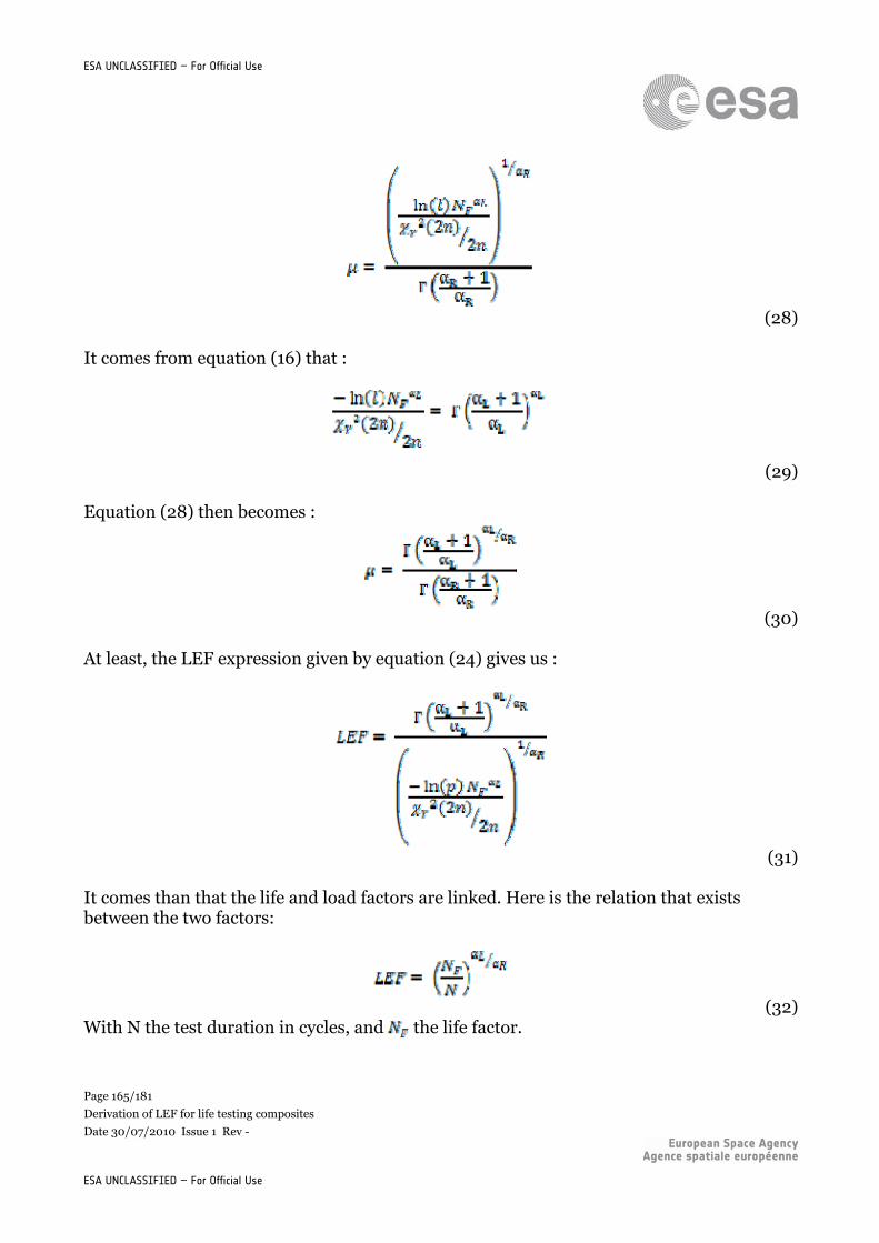
Page 165/181





(28)

It comes from equation (16) that :

(29)

Equation (28) then becomes :

(30)

At least, the LEF expression given by equation (24) gives us :

(31)

It comes than that the life and load factors are linked. Here is the relation that exists between the two factors:

(32)

With N the test duration in cycles, and the life factor.

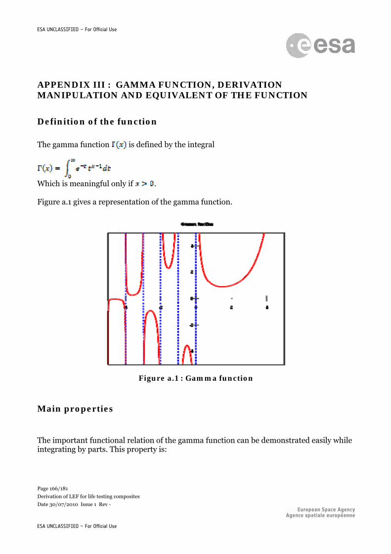
Page 166/181





APPENDIX III : GAMMA FUNCTION, DERIVATION MANIPULATION AND EQUIVALENT OF THE FUNCTION

Definition of the function

The gamma function is defined by the integral

Which is meaningful only if . Figure a.1 gives a representation of the gamma function.

Figure a.1 : Gamma function

Main properties

The important functional relation of the gamma function can be demonstrated easily while integrating by parts. This property is:

Page 167/181





(33)

It comes than that:

x=0,1,2,…,n

(34)

Computing values of the gamma function. In order to compute values of the LEF, one need to be able to compute values of the gamma function. Matlab gives exact values of the gamma function thanks to the “gamma” tool. Then the windows calculator can compute exact values using the (A2) relation. At least, Excel gives exact values using the tool “FACTGAMMA” available in a special Excel library to download, named GAMMA. But since it will be required to differentiate the gamma function, estimators are now going to be used. Two expressions of the gamma functions equivalents are given. The aim of the present study is to determine which expression better fits our needs. The first equivalent is the Stirling formula called “stirling” for the stydy given by:

(35)

The second equivalent called “approx” for the study is given by:

(36)

The first way to compare the two formulas and to know which better fits the gamma function is to plot the curves of the tree functions. Figure a.2 gives the plots of the tree curves.

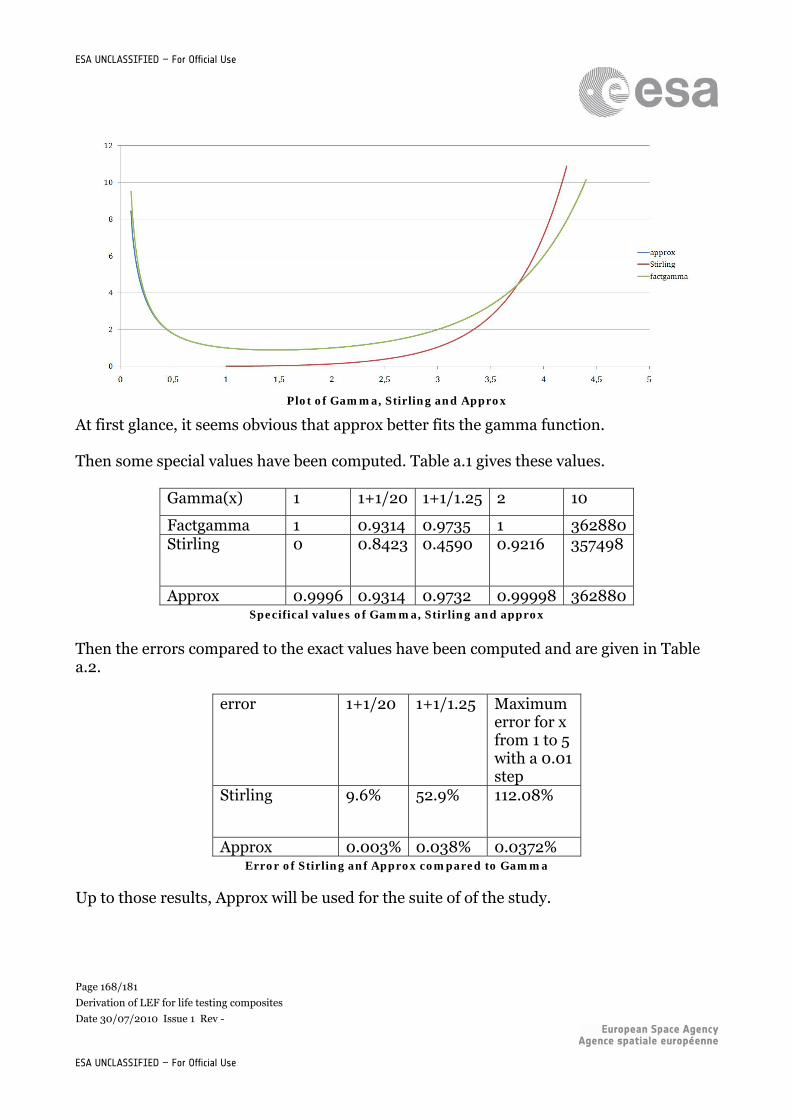
Page 168/181





Plot of Gamma, Stirling and Approx

At first glance, it seems obvious that approx better fits the gamma function. Then some special values have been computed. Table a.1 gives these values.

Gamma(x) 1 1+1/20 1+1/1.25 2 10

Factgamma 1 0.9314 0.9735 1 362880 Stirling 0 0.8423 0.4590 0.9216 357498

Approx 0.9996 0.9314 0.9732 0.99998 362880 Specifical values of Gamma, Stirling and approx

Then the errors compared to the exact values have been computed and are given in Table a.2.

error 1+1/20 1+1/1.25 Maximum error for x from 1 to 5 with a 0.01 step

Stirling 9.6% 52.9% 112.08%

Approx 0.003% 0.038% 0.0372% Error of Stirling anf Approx compared to Gamma

Up to those results, Approx will be used for the suite of of the study.

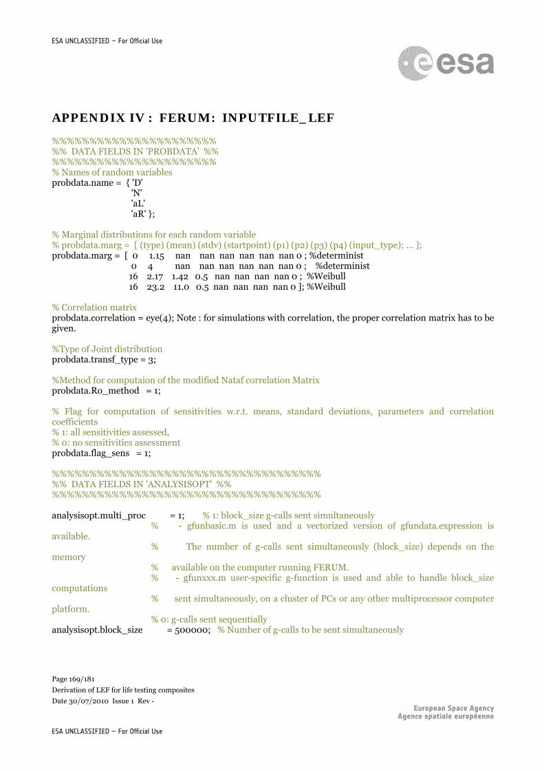
Page 169/181





APPENDIX IV : FERUM: INPUTFILE_LEF

%%%%%%%%%%%%%%%%%%%%%% %% DATA FIELDS IN 'PROBDATA' %% %%%%%%%%%%%%%%%%%%%%%% % Names of random variables probdata.name = { 'D' 'N' 'aL' 'aR' }; % Marginal distributions for each random variable % probdata.marg = [ (type) (mean) (stdv) (startpoint) (p1) (p2) (p3) (p4) (input_type); ... ]; probdata.marg = [ 0 1.15 nan nan nan nan nan nan 0 ; %determinist 0 4 nan nan nan nan nan nan 0 ; %determinist 16 2.17 1.42 0.5 nan nan nan nan 0 ; %Weibull 16 23.2 11.0 0.5 nan nan nan nan 0 ]; %Weibull % Correlation matrix probdata.correlation = eye(4); Note : for simulations with correlation, the proper correlation matrix has to be given. %Type of Joint distribution probdata.transf_type = 3; %Method for computaion of the modified Nataf correlation Matrix probdata.Ro_method = 1; % Flag for computation of sensitivities w.r.t. means, standard deviations, parameters and correlation coefficients % 1: all sensitivities assessed, % 0: no sensitivities assessment probdata.flag_sens = 1; %%%%%%%%%%%%%%%%%%%%%%%%%%%%%%%%%%%% %% DATA FIELDS IN 'ANALYSISOPT' %% %%%%%%%%%%%%%%%%%%%%%%%%%%%%%%%%%%%% analysisopt.multi_proc = 1; % 1: block_size g-calls sent simultaneously % - gfunbasic.m is used and a vectorized version of gfundata.expression is available. % The number of g-calls sent simultaneously (block_size) depends on the memory % available on the computer running FERUM. % - gfunxxx.m user-specific g-function is used and able to handle block_size computations % sent simultaneously, on a cluster of PCs or any other multiprocessor computer platform. % 0: g-calls sent sequentially analysisopt.block_size = 500000; % Number of g-calls to be sent simultaneously

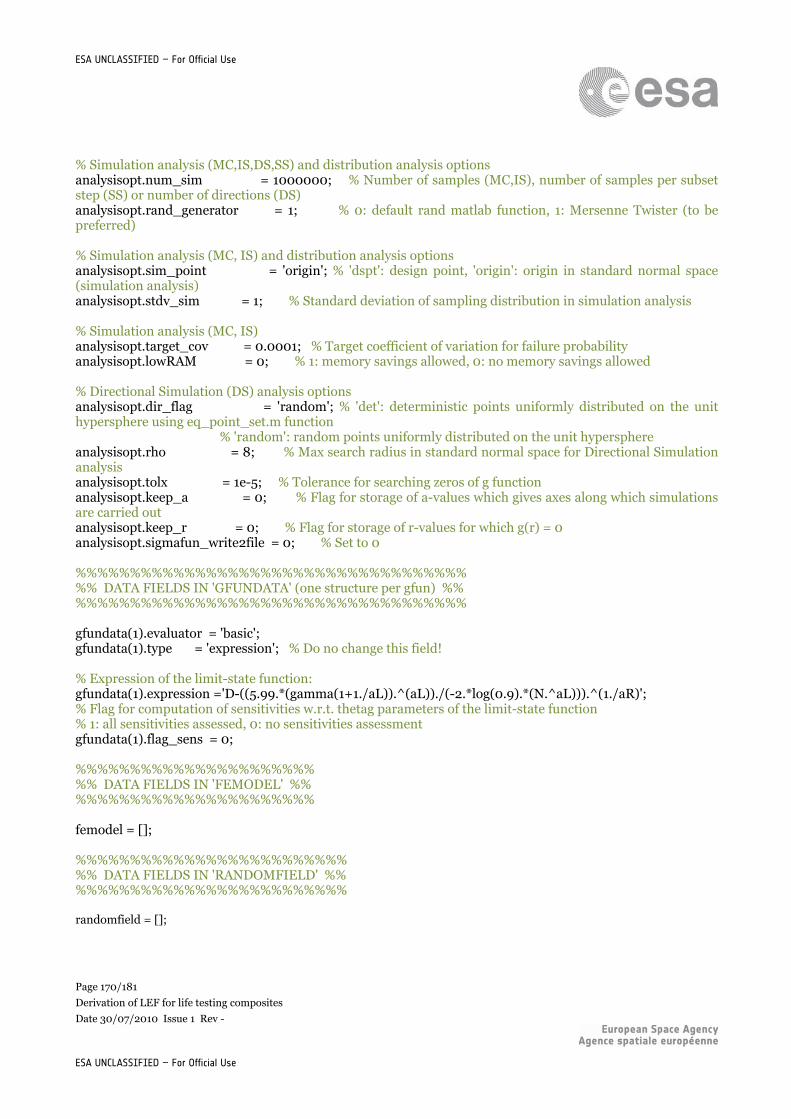
Page 170/181





% Simulation analysis (MC,IS,DS,SS) and distribution analysis options analysisopt.num_sim = 1000000; % Number of samples (MC,IS), number of samples per subset step (SS) or number of directions (DS) analysisopt.rand_generator = 1; % 0: default rand matlab function, 1: Mersenne Twister (to be preferred) % Simulation analysis (MC, IS) and distribution analysis options analysisopt.sim_point = 'origin'; % 'dspt': design point, 'origin': origin in standard normal space (simulation analysis) analysisopt.stdv_sim = 1; % Standard deviation of sampling distribution in simulation analysis % Simulation analysis (MC, IS) analysisopt.target_cov = 0.0001; % Target coefficient of variation for failure probability analysisopt.lowRAM = 0; % 1: memory savings allowed, 0: no memory savings allowed % Directional Simulation (DS) analysis options analysisopt.dir_flag = 'random'; % 'det': deterministic points uniformly distributed on the unit hypersphere using eq_point_set.m function % 'random': random points uniformly distributed on the unit hypersphere analysisopt.rho = 8; % Max search radius in standard normal space for Directional Simulation analysis analysisopt.tolx = 1e-5; % Tolerance for searching zeros of g function analysisopt.keep_a = 0; % Flag for storage of a-values which gives axes along which simulations are carried out analysisopt.keep_r = 0; % Flag for storage of r-values for which g(r) = 0 analysisopt.sigmafun_write2file = 0; % Set to 0 %%%%%%%%%%%%%%%%%%%%%%%%%%%%%%%%%%%% %% DATA FIELDS IN 'GFUNDATA' (one structure per gfun) %% %%%%%%%%%%%%%%%%%%%%%%%%%%%%%%%%%%%% gfundata(1).evaluator = 'basic'; gfundata(1).type = 'expression'; % Do no change this field! % Expression of the limit-state function: gfundata(1).expression ='D-((5.99.*(gamma(1+1./aL)).^(aL))./(-2.*log(0.9).*(N.^aL))).^(1./aR)'; % Flag for computation of sensitivities w.r.t. thetag parameters of the limit-state function % 1: all sensitivities assessed, 0: no sensitivities assessment gfundata(1).flag_sens = 0; %%%%%%%%%%%%%%%%%%%%%% %% DATA FIELDS IN 'FEMODEL' %% %%%%%%%%%%%%%%%%%%%%%% femodel = []; %%%%%%%%%%%%%%%%%%%%%%%%% %% DATA FIELDS IN 'RANDOMFIELD' %% %%%%%%%%%%%%%%%%%%%%%%%%% randomfield = [];

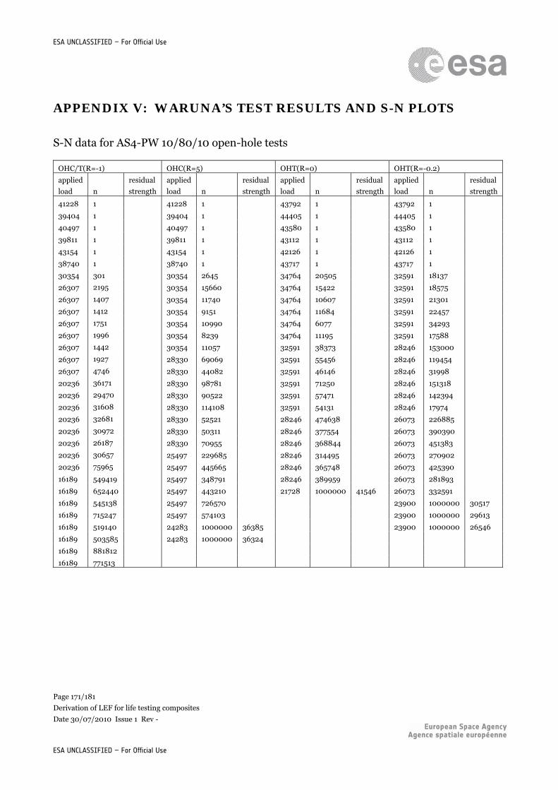
Page 171/181





APPENDIX V: WARUNA’S TEST RESULTS AND S-N PLOTS

S-N data for AS4-PW 10/80/10 open-hole tests

OHC/T(R=-1) OHC(R=5) OHT(R=0) OHT(R=-0.2)

applied

load n

residual

strength

applied

load n

residual

strength

applied

load n

residual

strength

applied

load n

residual

strength

41228 1 41228 1 43792 1 43792 1

39404 1 39404 1 44405 1 44405 1

40497 1 40497 1 43580 1 43580 1

39811 1 39811 1 43112 1 43112 1

43154 1 43154 1 42126 1 42126 1

38740 1 38740 1 43717 1 43717 1

30354 301 30354 2645 34764 20505 32591 18137

26307 2195 30354 15660 34764 15422 32591 18575

26307 1407 30354 11740 34764 10607 32591 21301

26307 1412 30354 9151 34764 11684 32591 22457

26307 1751 30354 10990 34764 6077 32591 34293

26307 1996 30354 8239 34764 11195 32591 17588

26307 1442 30354 11057 32591 38373 28246 153000

26307 1927 28330 69069 32591 55456 28246 119454

26307 4746 28330 44082 32591 46146 28246 31998

20236 36171 28330 98781 32591 71250 28246 151318

20236 29470 28330 90522 32591 57471 28246 142394

20236 31608 28330 114108 32591 54131 28246 17974

20236 32681 28330 52521 28246 474638 26073 226885

20236 30972 28330 50311 28246 377554 26073 390390

20236 26187 28330 70955 28246 368844 26073 451383

20236 30657 25497 229685 28246 314495 26073 270902

20236 75965 25497 445665 28246 365748 26073 425390

16189 549419 25497 348791 28246 389959 26073 281893

16189 652440 25497 443210 21728 1000000 41546 26073 332591

16189 545138 25497 726570 23900 1000000 30517

16189 715247 25497 574103 23900 1000000 29613

16189 519140 24283 1000000 36385 23900 1000000 26546

16189 503585 24283 1000000 36324

16189 881812

16189 771513

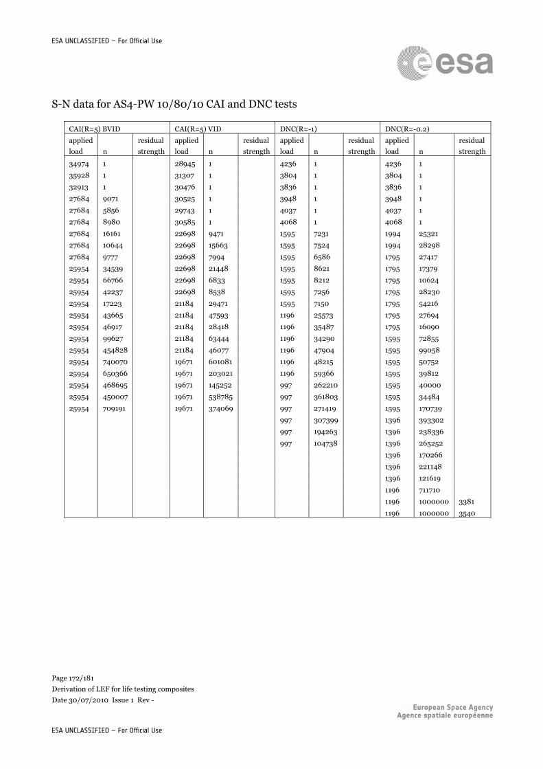
Page 172/181





S-N data for AS4-PW 10/80/10 CAI and DNC tests

CAI(R=5) BVID CAI(R=5) VID DNC(R=-1) DNC(R=-0.2)

applied

load n

residual

strength

applied

load n

residual

strength

applied

load n

residual

strength

applied

load n

residual

strength

34974 1 28945 1 4236 1 4236 1

35928 1 31307 1 3804 1 3804 1

32913 1 30476 1 3836 1 3836 1

27684 9071 30525 1 3948 1 3948 1

27684 5856 29743 1 4037 1 4037 1

27684 8980 30585 1 4068 1 4068 1

27684 16161 22698 9471 1595 7231 1994 25321

27684 10644 22698 15663 1595 7524 1994 28298

27684 9777 22698 7994 1595 6586 1795 27417

25954 34539 22698 21448 1595 8621 1795 17379

25954 66766 22698 6833 1595 8212 1795 10624

25954 42237 22698 8538 1595 7256 1795 28230

25954 17223 21184 29471 1595 7150 1795 54216

25954 43665 21184 47593 1196 25573 1795 27694

25954 46917 21184 28418 1196 35487 1795 16090

25954 99627 21184 63444 1196 34290 1595 72855

25954 454828 21184 46077 1196 47904 1595 99058

25954 740070 19671 601081 1196 48215 1595 50752

25954 650366 19671 203021 1196 59366 1595 39812

25954 468695 19671 145252 997 262210 1595 40000

25954 450007 19671 538785 997 361803 1595 34484

25954 709191 19671 374069 997 271419 1595 170739

997 307399 1396 393302

997 194263 1396 238336

997 104738 1396 265252

1396 170266

1396 221148

1396 121619

1196 711710

1196 1000000 3381

1196 1000000 3540

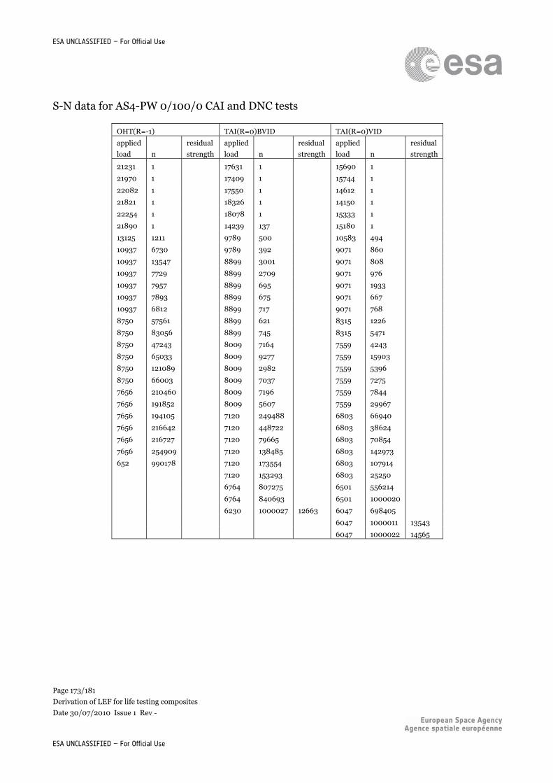
Page 173/181





S-N data for AS4-PW 0/100/0 CAI and DNC tests

OHT(R=-1) TAI(R=0)BVID TAI(R=0)VID

applied

load n

residual

strength

applied

load n

residual

strength

applied

load n

residual

strength

21231 1 17631 1 15690 1

21970 1 17409 1 15744 1

22082 1 17550 1 14612 1

21821 1 18326 1 14150 1

22254 1 18078 1 15333 1

21890 1 14239 137 15180 1

13125 1211 9789 500 10583 494

10937 6730 9789 392 9071 860

10937 13547 8899 3001 9071 808

10937 7729 8899 2709 9071 976

10937 7957 8899 695 9071 1933

10937 7893 8899 675 9071 667

10937 6812 8899 717 9071 768

8750 57561 8899 621 8315 1226

8750 83056 8899 745 8315 5471

8750 47243 8009 7164 7559 4243

8750 65033 8009 9277 7559 15903

8750 121089 8009 2982 7559 5396

8750 66003 8009 7037 7559 7275

7656 210460 8009 7196 7559 7844

7656 191852 8009 5607 7559 29967

7656 194105 7120 249488 6803 66940

7656 216642 7120 448722 6803 38624

7656 216727 7120 79665 6803 70854

7656 254909 7120 138485 6803 142973

652 990178 7120 173554 6803 107914

7120 153293 6803 25250

6764 807275 6501 556214

6764 840693 6501 1000020

6230 1000027 12663 6047 698405

6047 1000011 13543

6047 1000022 14565

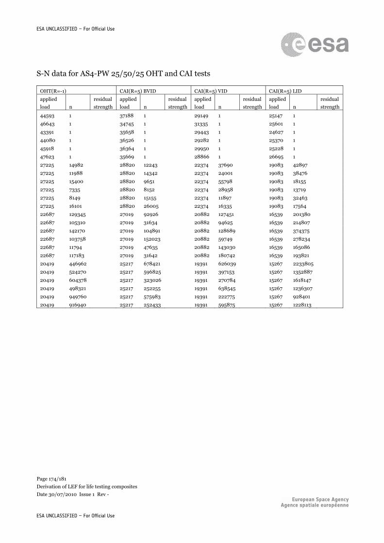
Page 174/181





S-N data for AS4-PW 25/50/25 OHT and CAI tests

OHT(R=-1) CAI(R=5) BVID CAI(R=5) VID CAI(R=5) LID

applied

load n

residual

strength

applied

load n

residual

strength

applied

load n

residual

strength

applied

load n

residual

strength

44593 1 37188 1 29149 1 25147 1

46643 1 34745 1 31335 1 25601 1

43391 1 35658 1 29443 1 24627 1

44080 1 36526 1 29282 1 25370 1

45918 1 36364 1 29950 1 25228 1

47623 1 35669 1 28866 1 26695 1

27225 14982 28820 12243 22374 37690 19083 42897

27225 11988 28820 14342 22374 24001 19083 38476

27225 15400 28820 9651 22374 55798 19083 18155

27225 7335 28820 8152 22374 28958 19083 13719

27225 8149 28820 15155 22374 11897 19083 32463

27225 16101 28820 26005 22374 16335 19083 17564

22687 129345 27019 92926 20882 127451 16539 201380

22687 105310 27019 31634 20882 94625 16539 214807

22687 142170 27019 104891 20882 128689 16539 374375

22687 103758 27019 152023 20882 59749 16539 278234

22687 11794 27019 47635 20882 143030 16539 165086

22687 117183 27019 31642 20882 180742 16539 193821

20419 446962 25217 678421 19391 626039 15267 2233805

20419 524270 25217 596825 19391 397153 15267 1352887

20419 604378 25217 323026 19391 270784 15267 1618147

20419 498321 25217 252255 19391 638545 15267 1236307

20419 949760 25217 575983 19391 222775 15267 928401

20419 916940 25217 252433 19391 595875 15267 1228113

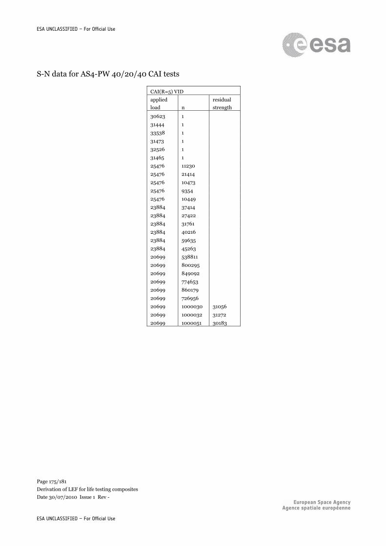
Page 175/181





S-N data for AS4-PW 40/20/40 CAI tests

CAI(R=5) VID

applied

load n

residual

strength

30623 1

31444 1

33538 1

31473 1

32526 1

31465 1

25476 11230

25476 21414

25476 10473

25476 9354

25476 10449

23884 37414

23884 27422

23884 31761

23884 40216

23884 59635

23884 45263

20699 538811

20699 800295

20699 849092

20699 774653

20699 860179

20699 726956

20699 1000030 31056

20699 1000032 31272

20699 1000051 30183

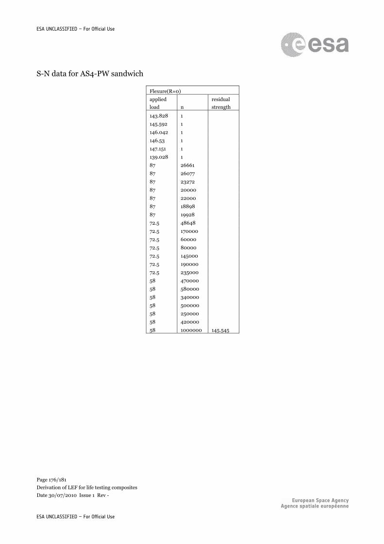
Page 176/181





S-N data for AS4-PW sandwich

Flexure(R=0)

applied

load n

residual

strength

143.828 1

145.592 1

146.042 1

146.53 1

147.151 1

139.028 1

87 26661

87 26077

87 23272

87 20000

87 22000

87 18898

87 19928

72.5 48648

72.5 170000

72.5 60000

72.5 80000

72.5 145000

72.5 190000

72.5 235000

58 470000

58 580000

58 340000

58 500000

58 250000

58 420000

58 1000000 145.545

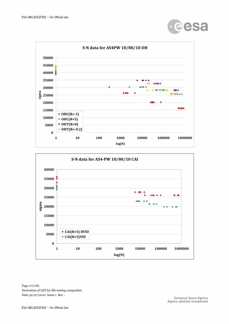
Page 177/181





SN data for AS4PW 10/80/10 OH

0

5000

10000

15000

20000

25000

30000

35000

40000

45000

50000

1 10 100 1000 10000 100000 1000000

log(N)

sigm

a

OHC(R=1)OHC(R=5)OHT(R=0)OHT(R=0.2)

SN data for AS4PW 10/80/10 CAI

0

5000

10000

15000

20000

25000

30000

35000

40000

1 10 100 1000 10000 100000 1000000

log(N)

sigm

a

CAI(R=5) BVIDCAI(R=5)VID

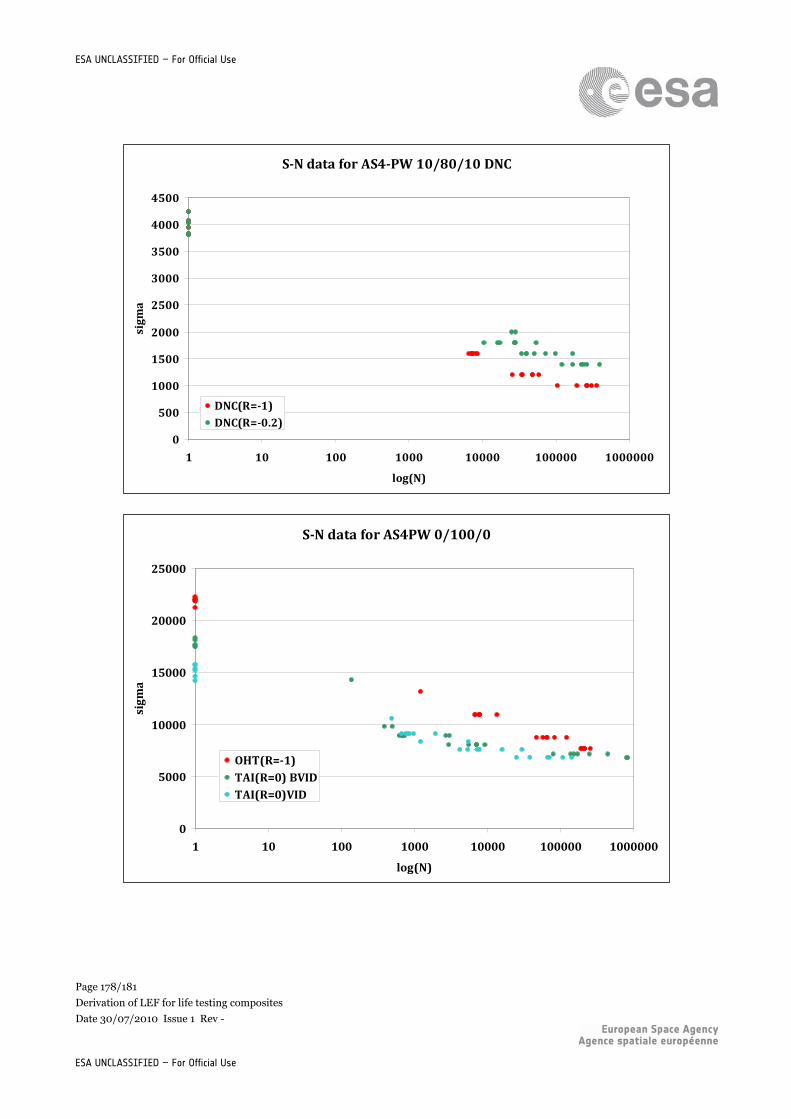
Page 178/181





SN data for AS4PW 10/80/10 DNC

0

500

1000

1500

2000

2500

3000

3500

4000

4500

1 10 100 1000 10000 100000 1000000

log(N)

sigm

a

DNC(R=1)DNC(R=0.2)

SN data for AS4PW 0/100/0

0

5000

10000

15000

20000

25000

1 10 100 1000 10000 100000 1000000

log(N)

sigm

a

OHT(R=1)TAI(R=0) BVIDTAI(R=0)VID

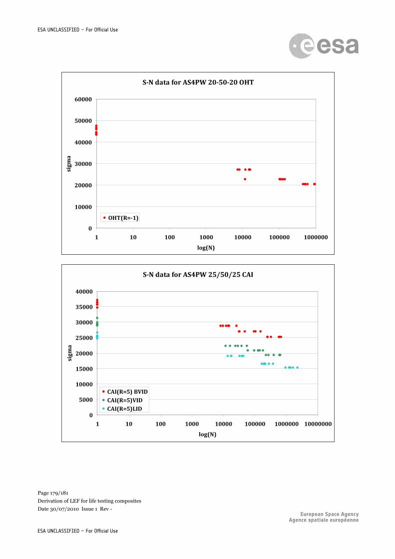
Page 179/181





SN data for AS4PW 205020 OHT

0

10000

20000

30000

40000

50000

60000

1 10 100 1000 10000 100000 1000000

log(N)

sigm

a

OHT(R=1)


0

5000

10000

15000

20000

25000

30000

35000

40000

1 10 100 1000 10000 100000 1000000 10000000

log(N)

sigm

a

CAI(R=5) BVIDCAI(R=5)VIDCAI(R=5)LID

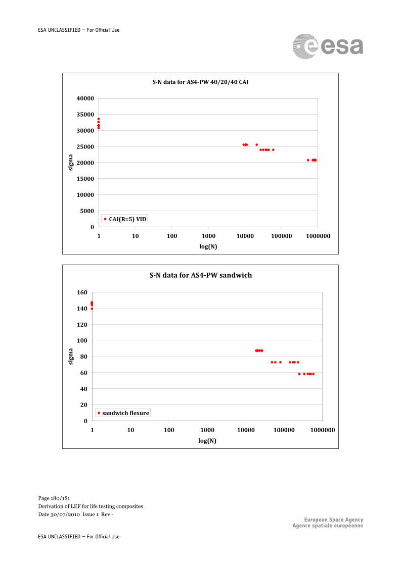
Page 180/181






0

5000

10000

15000

20000

25000

30000

35000

40000

1 10 100 1000 10000 100000 1000000

log(N)

sigm

a

CAI(R=5) VID

SN data for AS4PW sandwich

0

20

40

60

80

100

120

140

160

1 10 100 1000 10000 100000 1000000

log(N)

sigm

a

sandwich flexure

Page 181/181





Documents

The derivation of Load Enhancement Factors for life …emits.sso.esa.int/emits-doc/ESTEC/8042_RD48FinalReportV...APPENDIX II : Life factor and Load enhancement factor derivation.....162