The Design of Fiscal Adjustments - The National Bureau of ... · 2 The Design of Fiscal Adjustments Alberto Alesina, Harvard University, IGIER, and NBER Silvia Ardagna, Goldman Sachs

This PDF is a selection from a published volume from the National Bureau of Economic Research

Volume Title: Tax Policy and the Economy, Volume 27

Volume Author/Editor: Jeffrey R. Brown, editor

Volume Publisher: University of Chicago Press

Volume ISBN: paper 978-0-226-09779-4, cloth 978-0-226-09779-4; e-book 978-0-226-09782-4

ISSN: 0892-8649

Volume URL: http://www.nber.org/books/brow12-1

Conference Date: September 20, 2012

Publication Date: October 2013

Chapter Title: "The Design of Fiscal Adjustments"

Chapter Author(s): Alberto Alesina, Silvia Ardagna

Chapter URL: http://www.nber.org/chapters/c12853

Chapter pages in book: (p. 19 - 67)

http://www.jstor.org/action/showPublisher?publisherCode=ucpress

http://www.jstor.org/stable/10.1086/671243?origin=JSTOR-pdf

http://www.jstor.org/page/info/about/policies/terms.jsp


2

The Design of Fiscal Adjustments

Alberto Alesina, Harvard University, IGIER, and NBER

Silvia Ardagna, Goldman Sachs

Executive Summary

This paper offers three results. First, in line with the previous literature, we con-firm that fiscal adjustments basedmostly on the spending side are less likely to bereversed. Second, spending-based fiscal adjustments have caused smaller reces-sions than tax-based fiscal adjustments. Finally, certain combinations of policieshavemade it possible for spending-based fiscal adjustments to be associatedwithgrowth in the economy even on impact rather thanwith a recession. Thus, expan-sionary fiscal adjustments are possible.

I. Introduction

There are two critical questions regarding fiscal adjustments, defined asdecisive reductions of government deficits. First, what is the effectivemixbetween tax increases and spending cuts in order to achieve a relativelypermanent reduction of the debt/GDP ratio? We define this as a “suc-cessful” fiscal adjustment. Second, how large are the output and employ-ment losses associatedwith fiscal adjustments? Is it possible to completelyeliminate them?This paper offers new evidence on these questions. We find the follow-

ing results. First, in line with the previous literature, we confirm that fis-cal adjustments based mostly on the spending side have been less likelyto be reversed and have led to more long-lasting reductions of debt overGDP ratios. Second, expenditure-based fiscal adjustments are correlatedwith smaller recessions than tax-based fiscal adjustments. In some cases,during and in the immediate aftermath of spending-based fiscal adjust-ments, GDP growth is actually higher than in the years before. These epi-sodes of “expansionary” fiscal adjustments aremore likely to occurwhenthey are accompanied by a growth-oriented policy mix such as labormarket and goods market liberalization. A sense of “regime change” in

B 2013 by the National Bureau of Economic Research. All rights reserved.
978-0-226-09779-4/2013/2013-0002$10.00
This content downloaded from 23.235.32.0 on Tue, 10 Nov 2015 09:11:01 AMAll use subject to JSTOR Terms and Conditions


which expectations are turned around may also be important and may

Alesina and Ardagna20

affect investors’ confidence.The present paper builds on a rich and lively literature based on “epi-

sodes.” The first paper in this series was by Giavazzi and Pagano (1990),who studied the experience of Denmark in the early 1980s and Ireland atthe end of the same decade and argued that these episodes representcases of “expansionary fiscal adjustments.” The argument was that anincrease in consumers’ and investors’ confidence, associated with thedrastic fiscal change and reflected in a sharp fall in long-term interestrates, compensated the Keynesian effect of tax hikes and spending cuts.A large literature has followed that paper making two points: first,spending-based adjustments are less contractionary and are more likelyto lead to a permanent stabilization or a reduction of the debt to GDPratio; second, in some cases spending-based adjustments have been as-sociatedwith no recession at all, even in the short run, thus producing anexpansionary fiscal adjustment. The first paper looking at the universe oflarge fiscal adjustments was Alesina and Perotti (1995). Many other pa-pers followed along similar lines confirming those results.1

One difficult issue in this literature is how to identify episodes of largediscretionary policy changes. Up until a paper by Alesina and Ardagna(2010), the identification criteria were based on observed outcomes: alarge fiscal adjustment was one in which the cyclically adjusted primarydeficit over GDP ratio fell by a certain amount (normally at least 1.5% ofGDP). The results are not unduly sensitive to the choice of the threshold.The idea was that such a large adjustment in the cyclically adjusted pri-mary deficit was unlikely to be driven by the business cycle and was, in-stead, an indication of a discretionary active fiscal adjustment package. Arecent paper by economists at the International Monetary Fund (IMF2010) suggested a different way of identifying large, exogenous fiscal ad-justments. Following the narrative approach pioneered by Romer andRomer (2010), they picked cases that according to their criteria were at-tempts by governments to reduce deficits aggressively. Although the pre-sentation of that paper emphasized the differences with earlier work, thefindings were essentially in line with the results summarized by Alesinaand Ardagna (2010) in the sense that both agree that spending-based ad-justments lead to much smaller downturns in output. The IMF studyfinds that, on average, in the episodes their identification technique picksup, adjustments in the short run cause (modest) recessions. The IMF find-ings, however, have been revisited, and a later IMF paper (Devries et al.2011), using the same methodology, revised the set of fiscal stabilizationepisodes (see Favero, Giavazzi, and Perego [2011] for a comparison of the



results obtained using the two sets of data). About a third of the episodes

Design of Fiscal Adjustments 21

are reclassified from the 2010 to the 2011 version. We consider the laterrevisions as the correct and final version of episodes. Alesina, Favero,and Giavazzi (2012) show using the IMF definitions that the results re-garding the composition of spending versus tax changes are robust.Spending cuts have been associated with very small or no recessionswhile tax increases have been associated with large recessions. Boththe current paper and Alesina et al. (2012) find that, contrary to the claimby IMF (2010) and Devries et al. (2011), monetary policy is not the expla-nation of the systematic differences between tax-based and expenditure-based adjustments.But there are other possible policies. In fact Alesina and Ardagna

(1998) and Perotti (2013) note that fiscal adjustments are multiyear richpolicy packages and that one can learn a lot from detailed case studies.One lesson of these case studies is that several accompanying policies (inaddition to spending cuts or tax increases) favor the success of a fiscaladjustment and can moderate the contractionary effects on the economy.For instance, income policies (wage agreements) help, and such policiesare helped by fiscal programs that slow down the dynamics of public-sector wages. Wage moderation and sometimes, but schematically, ex-change rate devaluation help competitiveness, inducing an export boom.The behavior of private investment is often central if entrepreneurs reactpositively to a change in the fiscal package (Alesina et al. 2002, 2012).As far as the channels through which fiscal adjustments can affect the

economy, the appropriate policy mix has effects on the economy both onthe demand side and on the supply side of the economy. The relativelysmall negative effects of spending cuts on growth via the demand sidecan be compensated by the positive effect that accommodativemonetarypolicies have on the demand side and/or by the positive effect that cutsto current spending and liberalization reforms have via the supply sideof the economy. In some cases, expectations about a change in the policyregime generated a positive wealth effect and a reduction in risk premiaon long-term interest rates. This had positive effects on private consump-tion and investment.Whilewe do not test for the channels throughwhichfiscal adjustments affect the economy in this paper, we have done so inour previous research. In particular, Alesina et al. (2002) show thatspending cuts have a positive effect on private investment while in-creases in taxes, particularly labor taxes, hurt investment through thelabor market and firms’ profitability. The size of fiscal policy shockson firms’ profits and private investment is large enough to explain theboom (fall) in private investment that accompanied expansionary and



spending-based (contractionary and tax-based) fiscal adjustments.


Hence, we concluded that there might be nothing special around largefiscal adjustments in terms of the reaction of expectations but that thecomposition of the adjustment and its effects on the labor markets canexplain the different outcomes. A similar conclusion is also reached byArdagna (2004) that running a horse race between the so-called expecta-tion channel and the labor market channel finds more evidence in favorof the latter than the former. Finally, Alesina and Perotti (1995) find evi-dence that spending cuts have a positive effect on exports’ competitive-ness, while increases in taxeswork in the opposite direction. See also Finn(1998), Daveri and Tabellini (2000), and Ardagna (2007) for models thatformalize the effects of changes to the government wage bills, transfers,and labor tax increases on the economy in the context of unionized orperfectly competitive labor markets.The present paper takes on from this line of papers. It uses both the

IMF classification of fiscal adjustments and the earlier one based on thesize of changes of the cyclically adjusted primary deficit over GDP ratio.We try to clarify the differences between the two both methodologicallyand empirically. In addition, we expand the analysis to include the effectsof a vast set of policies that constitute the “package” accompanying thefiscal cuts. By considering many alternative definitions of fiscal adjust-ments, we can do many robustness checks on our previous results andconfirm that they are robust. The main result we obtain is that the keymessage regarding the composition of fiscal adjustments is the same re-gardless of the definition used to identify episodes of fiscal adjustments(i.e., our definition using actual outcomes on the cyclically adjusted def-icit and the IMF definition based on announced plans for cuts). The sameresult is obtained by the vector autoregression analysis of Alesina et al.(2012), who focus in particular on the confidence channel, and by Biggs,Hasset, and Jensen (2010).Before proceeding, it isworthmentioning two disclaimers. First, we do

not plan to review here the vast recent literature on empirical fiscal pol-icy, the size of spending multipliers, and so forth. We refer to severalchapters in Alesina and Giavazzi (2013) for this task. Second, we offerno policy discussion on the size, timing, and opportunity of the currentfiscal adjustments in Europe or the United States. The reader can drawhis or her own conclusion on the basis of the historical evidence and em-pirical analysis we present.2

This paper is organized as follows. In Section II, we discuss data anddefinitional issues. In particular, we consider alternative definitionsof what a fiscal adjustment is. In Section III, we use our outcome-based



definition to investigate successful and expansionary adjustments versus


unsuccessful and contractionary ones. Section III also discusses the pol-icymix that leads to success versus failure. Section IVuses theWorld Eco-nomic Outlook definition of fiscal adjustments and repeats the sameanalysis of success versus failure. Section V provides econometric evi-dence on the effect of different types of fiscal adjustments on the economyusing the samemethodology proposed by the IMF (2010). Section VI pre-sents conclusions.

II. Data and Definitions

A. Data

We consider data on 21 OECD countries from 1970 to 2010. The countriesincluded in the sample areAustralia,Austria, Belgium,Canada,Denmark,France, Finland, Germany, Greece, Italy, Ireland, Japan, the Netherlands,New Zealand, Norway, Portugal, Spain, Sweden, Switzerland, the UnitedKingdom, and theUnited States.3 The variables’definitions and the sourceof the variables are indicated in table 1.

B. Definitions of Fiscal Adjustments

Defining an episode of fiscal adjustment is challenging for two reasons.The first difficulty lies in the endogeneity of fiscal variables; that is, thereduction of the deficit over GDP ratio may be due to an increase in thedenominator andmay have nothing to dowith a discretionary policy ac-tion. Obviously, one can (and should) use cyclically adjusted fiscal vari-ables, but the cyclical correction is notoriously imperfect and arbitrary tosome extent. Thus, one has to worry about the fact that in a boom, notonly may spending go down because of automatic stabilizers but thegovernmentmay choose to cut discretionary spending. Second, it is oftendifficult to identify the precise timing since fiscal adjustments are oftenmultiyear events. For instance, imagine a country in which the deficitover GDP ratio falls by 2% in year t, by 0.1% in year tþ 1, and by 2%in year tþ 2. Does one consider the 3-year period one fiscal adjustmentor does one consider year t and year tþ 2 as two separate episodes?Depending on what choice one makes, the results might be different.The literature on episodes adopted definitions that considered only

single-year large adjustments or consecutive years in which the adjust-ment in each year was smaller but always in the range of 1%–2% as thisrange seemed a high enough one to isolate large episodes but not so large



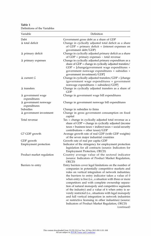
Table 1Definitions of the Variables

Variable Definition

DebtΔ total deficit

Δ current G

G7 GDP growth

This content downloadeAll use

Government gross debt as a share of GDPChange in cyclically adjusted total deficit as a share
of GDP = primary deficit + (interest expenses ongovernment debt/GDP)
Δ primary deficit
Change in cyclically adjusted primary deficit as a shareof GDP = primary expenses − total revenue
Change in cyclically adjusted primary expenditure as a
Δ primary expenses share of GDP = change in cyclically adjusted transfers/GDP + [change(government wage expenditures + government nonwage expenditures + subsidies +government investment)/GDP]
Change in cyclically adjusted transfers/GDP + [change(government wage expenditures + governmentnonwage expenditures + subsidies)/GDP]

Δ transfers
Change in cyclically adjusted transfers as a share ofGDP
Change in government wage bill expenditures
Δ government wageexpenditures
Change in government nonwage bill expenditures
Δ government nonwageexpenditures
Subsidies
Δ government investment
Change in subsidies to firmsChange in gross government consumption on fixed

Total revenue
capital
Tax = change in cyclically adjusted total revenue as a
share of GDP = change in cyclically adjusted (incometaxes + business taxes + indirect taxes + social security contributions + other taxes)/GDP
Average growth rate of real GDP (with GDP weights)of the seven major industrial countries

Growth rate of real per capita GDP
GDP growthEmployment protection Indicator of the stringency for employment protection
legislation for all contracts (source: Indicators for
Employment Protection, OECD)
Product market regulation
Country average value of the sectoral indicator(source: Indicators of Product Market Regulation,OECD)
Barriers to entry
Entry barriers cover legal limitations on the number ofcompanies in potentially competitive markets andrules on vertical integration of network industries; the barriers to entry indicator takes a value of 0when entry is free (i.e., a situation with three or morecompetitors and with complete ownership separa-tion of natural monopoly and competitive segmentsof the industry) and a value of 6 when entry is se-verely restricted (i.e., situations with legal monopolyand full vertical integration in network industriesor restrictive licensing in other industries) (source:Indicators of Product Market Regulation, OECD)
(continued)

d from 23.235.32.0 on Tue, 10 Nov 2015 09:11:01 AMsubject to JSTOR Terms and Conditions


as to have too few episodes.4 The rationale for these definitions is that

Table 1Continued

Variable Definition

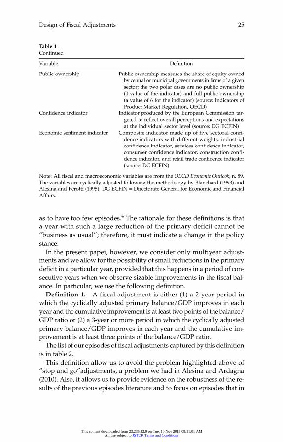
Public ownership Public ownership measures the share of equity ownedby central or municipal governments in firms of a givensector; the two polar cases are no public ownership(0 value of the indicator) and full public ownership(a value of 6 for the indicator) (source: Indicators ofProduct Market Regulation, OECD)

Confidence indicator Indicator produced by the European Commission tar-geted to reflect overall perceptions and expectationsat the individual sector level (source: DG ECFIN)

Economic sentiment indicator Composite indicator made up of five sectoral confi-dence indicators with different weights: industrialconfidence indicator, services confidence indicator,consumer confidence indicator, construction confi-dence indicator, and retail trade confidence indicator(source: DG ECFIN)

Note: All fiscal and macroeconomic variables are from the OECD Economic Outlook, n. 89.The variables are cyclically adjusted following the methodology by Blanchard (1993) andAlesina and Perotti (1995). DG ECFIN = Directorate-General for Economic and FinancialAffairs.


a year with such a large reduction of the primary deficit cannot be“business as usual”; therefore, it must indicate a change in the policystance.In the present paper, however, we consider only multiyear adjust-

ments andwe allow for the possibility of small reductions in the primarydeficit in a particular year, provided that this happens in a period of con-secutive years when we observe sizable improvements in the fiscal bal-ance. In particular, we use the following definition.Definition 1. A fiscal adjustment is either (1) a 2-year period in

which the cyclically adjusted primary balance/GDP improves in eachyear and the cumulative improvement is at least two points of the balance/GDP ratio or (2) a 3-year or more period in which the cyclically adjustedprimary balance/GDP improves in each year and the cumulative im-provement is at least three points of the balance/GDP ratio.The list of our episodes of fiscal adjustments captured by this definition

is in table 2.This definition allow us to avoid the problem highlighted above of

“stop and go”adjustments, a problem we had in Alesina and Ardagna(2010). Also, it allows us to provide evidence on the robustness of the re-sults of the previous episodes literature and to focus on episodes that in



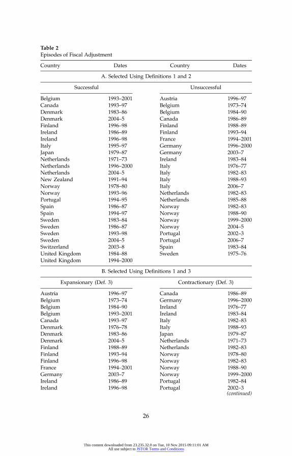
Table 2Episodes of Fiscal Adjustment

Country Dates Country Dates

A. ing Defin

B.

This content d

Selected Us

ing Defin

ownloaded from 23.235.32.0 on All use subject to JSTOR Term

itions 1 and 2

Tue, 10 Nov 2015 09:11:01 AMs and Conditions

Successful Unsuccessful

Belgium 1993–2001Canada 1993–97

Austria 1996–97Belgium 1973–74

DenmarkDenmark

1983–862004–5

BelgiumCanada

1984–901986–89

Finland
1996–98 Finland 1988–89 Ireland 1986–89 Finland 1993–94 Ireland 1996–98 France 1994–2001 Italy 1995–97 Germany 1996–2000 Japan 1979–87 Germany 2003–7 Netherlands 1971–73 Ireland 1983–84 Netherlands 1996–2000 Italy 1976–77 Netherlands 2004–5 Italy 1982–83 New Zealand 1991–94 Italy 1988–93 Norway 1978–80 Italy 2006–7 Norway 1993–96 Netherlands 1982–83 Portugal 1994–95 Netherlands 1985–88 Spain 1986–87 Norway 1982–83 Spain 1994–97 Norway 1988–90 Sweden 1983–84 Norway 1999–2000 Sweden 1986–87 Norway 2004–5 Sweden 1993–98 Portugal 2002–3 Sweden 2004–5 Portugal 2006–7 Switzerland 2003–8 Spain 1983–84 United Kingdom 1984–88 Sweden 1975–76 United Kingdom 1994–2000
Selected Us
itions 1 and 3
Expansionary (Def. 3) Contractionary (Def. 3)

Austria 1996–97Belgium 1973–74

Canada 1986–89Germany 1996–2000

BelgiumBelgium

1984–901993–2001

IrelandIreland

1976–771983–84

Canada
1993–97 Italy 1982–83 Denmark 1976–78 Italy 1988–93 Denmark 1983–86 Japan 1979–87 Denmark 2004–5 Netherlands 1971–73 Finland 1988–89 Netherlands 1982–83 Finland 1993–94 Norway 1978–80 Finland 1996–98 Norway 1982–83 France 1994–2001 Norway 1988–90 Germany 2003–7 Norway 1999–2000 Ireland 1986–89 Portugal 1982–84 Ireland 1996–98 Portugal 2002–3
(continued)
(continued)
26


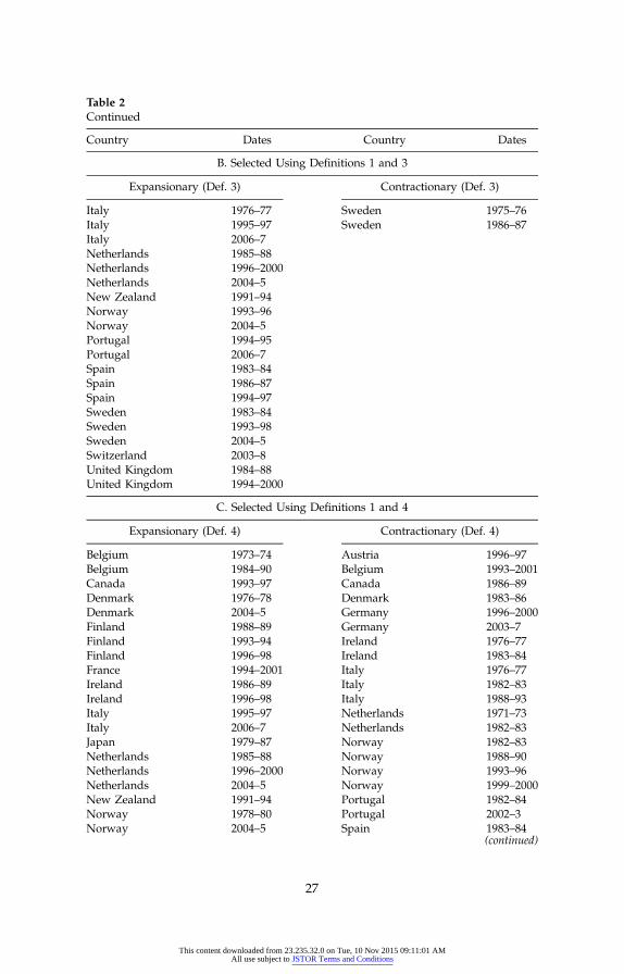
Table 2Continued


B. Selected Using Definitions 1 and 3


Italy 1976–77 Sweden 1975–76Italy 1995–97 Sweden 1986–87Italy 2006–7Netherlands 1985–88Netherlands 1996–2000Netherlands 2004–5New Zealand 1991–94Norway 1993–96Norway 2004–5Portugal 1994–95Portugal 2006–7Spain 1983–84Spain 1986–87Spain 1994–97Sweden 1983–84Sweden 1993–98Sweden 2004–5Switzerland 2003–8United Kingdom 1984–88United Kingdom 1994–2000

C. Selected Using Definitions 1 and 4


Belgium 1973–74 Austria 1996–97Belgium 1984–90 Belgium 1993–2001Canada 1993–97 Canada 1986–89Denmark 1976–78 Denmark 1983–86Denmark 2004–5 Germany 1996–2000Finland 1988–89 Germany 2003–7Finland 1993–94 Ireland 1976–77Finland 1996–98 Ireland 1983–84France 1994–2001 Italy 1976–77Ireland 1986–89 Italy 1982–83Ireland 1996–98 Italy 1988–93Italy 1995–97 Netherlands 1971–73Italy 2006–7 Netherlands 1982–83Japan 1979–87 Norway 1982–83Netherlands 1985–88 Norway 1988–90Netherlands 1996–2000 Norway 1993–96Netherlands 2004–5 Norway 1999–2000New Zealand 1991–94 Portugal 1982–84Norway 1978–80 Portugal 2002–3Norway 2004–5 Spain 1983–84

(continued)(continued)

27



terms of their duration are closer towhatOECDcountrieswill experience

Table 2Continued


C. Selected Using Definitions 1 and 4


Portugal 1994–95 Sweden 1975–76Portugal 2006–7 Sweden 1983–84Spain 1986–87 Sweden 2004–5Spain 1994–97 United Kingdom 1984–88Sweden 1986–87Sweden 1993–98Switzerland 2003–8United Kingdom 1994–2000


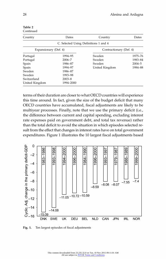
this time around. In fact, given the size of the budget deficit that manyOECD countries have accumulated, fiscal adjustments are likely to bemultiyear processes. Finally, note that we use the primary deficit (i.e.,the difference between current and capital spending, excluding interestrate expenses paid on government debt, and total tax revenue) ratherthan the total deficit to avoid the situation in which episodes selected re-sult from the effect that changes in interest rates have on total governmentexpenditures. Figure 1 illustrates the 10 largest fiscal adjustments based

Fig. 1. Ten largest episodes of fiscal adjustments



on this definition. Of the 52 episodes of fiscal adjustments, 24 last 2 years,


eight last 3 years, and the longest (only one) lasts 9 years.We are interested in twomeasures of results of fiscal adjustments. One

is whether they managed to reduce substantially the debt over GDPratio, and the second is a measure of costs in terms of downturn forthe economy.With regard to the first question, we label “successful” epi-sodes of fiscal adjustment that have led to a reduction of the debt/GDPratio and “unsuccessful” those with the opposite feature. We should em-phasize that one should not give a normative interpretation to this termbut simply consider it as a label that refers specifically to the effect of thefiscal adjustment on the debt/GDP ratio. We label “expansionary” thoseepisodes that have not led to a downturn and “recessionary” those thatdid. More precisely, we use the following definitions.Definition 2. A period of fiscal adjustment is successful if the debt to

GDP ratio 2 years after the end of a fiscal adjustment is lower than thedebt to GDP ratio in the last year of the adjustment.This definition selects 25 episodes of successful fiscal adjustments and

24 unsuccessful ones. Panel A of table 2 lists all the episodes.Definition 3. A period of fiscal adjustment is expansionary if real

GDP growth during the adjustment period is higher than the averagegrowth the country experienced in the 2 years before.This definition selects 35 episodes of expansionary fiscal adjust-

ments and 17 contractionary adjustments. Panel B of table 2 lists all theepisodes.In order to avoid the situation in which the world business cycle may

lead us to incorrectly classify adjustments because external factors maybe important for small open economies, we also use a second definitionto select expansionary and contractionary fiscal adjustments.Definition 4. An expansionary fiscal adjustment is one in which the

average growth in difference for the G7 average growth during the ad-justment was higher than the average growth in the 2 years before theadjustment relative to the G7 average growth.This definition isolates 28 cases of expansionary fiscal adjustments and

24 contractionary adjustments. Panel C of table 2 lists the episodes.We should be very clear on the following point. This correlation

between fiscal adjustments and the economy, which highlights the oc-currence of “expansionary” episodes, should not be considered “causal”at this point. We cannot say that austerity is growth promoting per se.We can only note at this point a correlation. In what follows we explorethis correlation to investigate whether certain types of fiscal adjustmentsrather than others are more likely to be contractionary or expansionary.



III. Different Types of Fiscal Adjustments


In this section we explore, on the basis of our two outcome defini-tions reported above, the characteristics of episodes distinguishing thosethat have been successful versus unsuccessful and expansionary versuscontractionary.

A. The Composition of Fiscal Adjustments

Table 3 presents some basic summary statistics on the successful versus un-successful episodes. Interestingly, they are almost exactly the same in num-ber (24 vs. 25). By definition the successful ones lead to a reduction of thedebt over GDP ratios and the others do not. Successful fiscal adjustmentswere slightly longer in time. More interestingly, successful fiscal adjust-ments were associated with higher growth during the adjustment. Need-less to say the higher growth is what might have helped in making theadjustment successful in the first place. In terms of world business cycleproxied by G7 growth, successful and unsuccessful adjustments are in-distinguishable. This hints to the fact that success or failure depends ondomestic factors rather than on the world business cycle. More on thisbelow.Table 4 shows some basis statistics regarding expansionary versus con-

tractionary episodes using our twodefinitions: panel A using definition 3

Table 3Successful versus Unsuccessful Fiscal Stabilizations

Successful UnsuccessfulSE of

Difference

Change in the debt/GDPDebt/GDP (tþ 2) − Debt/GDP (t)

ints oact de

This content downloaded from 23.All use subject to J

−.19−7.4

ss indthe v

235.32.0 on Tue, 10 Nov 2STOR Terms and Conditi

1.496.89

e du

015 09:11:01 AMons

.65**1.18***

GDP growthG7 GDP growth

3.472.89

2.32.89

.27***

.17
GDP growth in deviation from
G7 growth
.58 −.59 .25*** Average growth (t − t ) − average 0 n
growth (t0 − 2 − t0 − 1)Average duration

1.43
.32 .49**
Number of episodes
3.0325
2.5524

.28*

Note: Changes are in percentage po
f GDP unle icated. Averag ration is in terms of years. See table 1 for the ex finitions of ariables. *1% significance level.**5% significance level.***10% significance level.

and panel B using definition 4. As mentioned above, according to defini-

Table 4Expansionary versus Contractionary Fiscal Stabilizations

Change in the debt/GDP

Change in the debt/GDP

ri i


tion 1, there were more expansionary than contractionary episodes(35 vs. 17). According to the second, there were about half and half(28 vs. 24). Note how the G7 growth is virtually identical, on average, forall types of fiscal adjustments.Panel A of table 5 presents evidence on the composition of the episodes

of fiscal adjustments using definition 3. The key observation here is thatthere is a significant difference between successful and unsuccessful andcontractionary versus expansionary: the successful and expansionaryoneswere those basedmostly on spending cuts rather than on tax increases.This is the same result we had obtained earlier in Alesina and Ardagna(2010). All the components of spending except for public investment arereduced more during successful than unsuccessful adjustment. Publicemployment grows less in successful adjustments. All these differences

Expansionary ContractionarySE of

Difference

This content downloaded from 23.235.3All use subject to JSTOR

A

2.0 on Tue, 10 Nov 201 Terms and Conditions

. Definition 3

5 09:11:01 AM

Debt/GDP (tþ 2) − debt/GDP (t)
.34 1.1 .73
−1.88 2.94 2.5*
3.152.95

2.492.84

.31**

.18
GDP growth in deviation from G7 growth .2 −.35 .30* Average growth (t0 − tn) − average growth
(t0 − 2 − t0 − 1)
1.88 −1.25 .35*** Average duration 2.85 2.63 .3 Number of episodes 35 17
B
. Definition 4
Debt/GDP (tþ 2) − debt/GDP (t)
.54 .57 .66
−2.51 2.19 2.30**
3.312.86

2.462.99

.28***

.16
GDP growth in deviation from G7 growth .45 −.53 .27*** Average growth (t0 − tn) − average growth
(t0 − 2 − t0 − 1)
1.42 −1.39 .32*** Average duration 2.94 2.57 .27 Number of episodes 28 24
Note: Changes are in percentage points of G
DP unless indic ated. Average du ation is in terms of years. See table 1 for the exact defin tions of the var ables. *1% significance level.**5% significance level.***10% significance level.

Table

5Com

position

ofFiscal

Adjustmen

ts

Successful

Unsuc

cessful

SEof

Differen

ceExp

ansion

ary

Con

traction

ary

SEof

Differen

ce

A.D

efinition3

Δtotaldeficit

−6.27

−3.91

.80***

−5.43

−4.16

.86

Δprim

arydeficit

−5.82

−4.59

.83

−5.34

−4.8

.86

Δprim

aryexpe

nditures

−4.18

−2.53

.91*

−3.98

−2.05

.92**

Δcu

rren

tprim

arysp

ending

−2.48

−1.31

.73

−2.62

−.38

.68***

Δgo

vernmen

tconsum

ption

−1.35

−.61

.37**

−1.32

−.25

.36***

Δgo

vernmen

twag

eexpe

nditures

−1.1

−.59

.27*

−1.12

−.28

.26***

Δgo

vernmen

tno

nwag

eexpe

nditures

−.24

−.05

.2−.24

.03

.2Δ

tran

sfers

−.74

−.55

.4−.97

.04

.39**

Δsu

bsidies

−.39

−.15

.14*

−.33

−.17

.14

Δgo

vernmen

tinve

stmen

t−1

.7−1

.21

.5−1

.36

−1.67

.5Δ

totalreve

nue

1.64

2.06

.61.36

2.75

.58**

Com

position

—sp

ending

71.81

44.96

14.4*

71.14

33.98

14.18**

Com

position

—cu

rren

tsp

ending

45.36

20.75

14.8*

48.7

1.29

14.00***

Com

position

—capitalsp

ending

26.45

24.2

5.9

22.43

32.69

5.79

*Com

position

—taxes

28.19

55.04

14.4*

28.86

66.02

14.18**

Public

employ

men

tgrow

th1.64

3.08

1.62

1.51

6.37

1.84

**

32



B.D

efinition4

Δtotaldeficit

−5.62

−4.31

.81

Δprim

arydeficit

−5.49

−4.78

.8Δ

prim

aryexpe

nditures

−3.89

−2.72

.88

Δcu

rren

tprim

arysp

ending

−2.39

−1.29

.69

Δgo

vernmen

tconsum

ption

−1.26

−.63

.36*

Δgo

vernmen

twag

eexpe

nditures

−1.18

−.46

.25***

Δgo

vernmen

tno

nwag

eexpe

nditures

−.13

−.17

.19

Δtran

sfers

−.77

−.49

.39

Δsu

bsidies

−.37

−.17

.13

Δgo

vernmen

tinve

stmen

t−1

.49

−1.42

.47

Δtotalreve

nue

1.6

2.07

.57

Com

position

—sp

ending

66.56

50.16

14.04

Com

position

—cu

rren

tsp

ending

42.33

22.56

14.3

Com

position

—capitalsp

ending

24.24

27.59

5.6

Com

position

—taxes

33.44

49.84

14.04

Public

employ

men

tgrow

th1.84

4.8

1.83

Note:The

tablerepo

rtsthecu

mulativech

ange

inva

riab

lesof

interestov

ertheep

isod

eof

fiscalad

justmen

t.Cha

nges

arein

percen

tage

pointsof

GDPun

less

indicated

.Com

position

—sp

ending,

compo

sition

—cu

rren

tspe

nding,

compo

sition

—capitalspe

nding,

andcompo

sition

—taxesarech

ange

sin

theresp

ec-

tive

variab

lesin

percen

tage

pointsof

thech

ange

ofprim

arydeficit.P

ublic

employ

men

tgrowth

isin

percen

tage

points.See

table1forthe

exactd

efinitions

oftheva

riab

les.

*1%

sign

ifican

celeve

l.**5%

sign

ifican

celeve

l.***10%

sign

ifican

celeve

l.

33



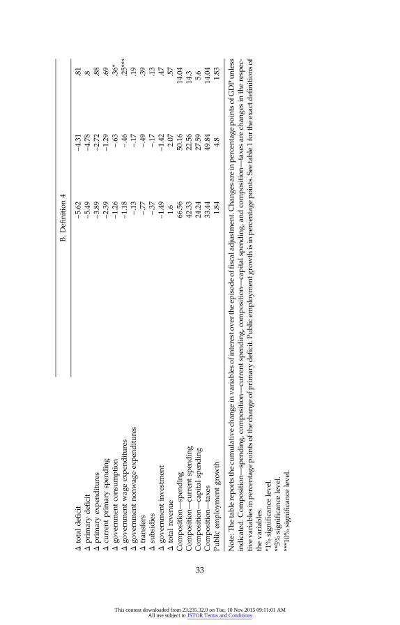
are statistically significant at standard conventional levels. Interestingly,


the size of the reduction of the cyclically adjusted deficit is virtually iden-tical for expansionary and contractionary adjustments while, perhapsnot surprisingly, the size is much larger for successful ones versus un-successful ones. A breakdown of different types of taxes does not yieldsignificant differences (results are available from the authors). More de-tailed research on this point is warranted.Note that when comparing successful versus unsuccessful adjust-

ments, it is apparent that the reduction in total deficit is much larger thanthat of primary deficit. This indicates a strong reaction in interest rates,which may be due to investors’ confidence effects. Alesina et al. (2012)investigate more formally these confidence effects, finding that indeedconfidence “moves,” but it is unclear whether it follows or precedesmovement of output. Note also that the yearly reduction in the primarydeficit is lower than 2%, on average, and that although in successful andexpansionary adjustments the cumulative reduction of the primary def-icit is larger, its size is not statistically different from that in unsuccessfuland contractionary episodes.5 Panel B of table 5 uses definition 4 as a def-inition of expansionary versus contractionary episodes. The results arebroadly quite similar to those of panel A. From now on we use definition 3for all the other tables we present. The results using the other definitionsare quite similar and are available from the authors.Table 6 investigates differences in initial conditions. There do not seem

any statistically different initial conditions when comparing successfulversus unsuccessful episodes. Growth was higher for successful ones,but unemployment was also higher and the output larger. The resultsare striking for the case of expansionary versus contractionary episodes.In this case, it is pretty clear that expansionary episodes started withworse initial conditions, growth was lower, the output gap was larger,and unemployment was higher. There are two possible interpretationsof this result. One is that growth was picking up on its own and contin-ued to pick up “despite” the fiscal adjustment. This would imply that themeasures of cyclical adjustment on the deficits are imperfect. The otherinterpretation is that the fiscal adjustmentwas part of a package that gen-erated a “major change” in the policy stance that favored austerity andgrowth at the same time.6 The results presented in the next section pointtoward the second interpretation because the policymix of expansionaryfiscal adjustments included progrowth supply-side reforms. This inter-pretation would be consistent with the case studies analyzed by Alesinaand Ardagna (1998) and Perotti (2013). In their view, episodes of largefiscal adjustments are a complex combination of policy actions including



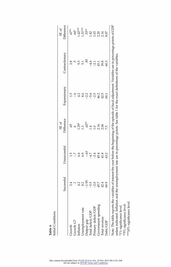
Table

6InitialC

onditions

Successful

Unsuc

cessful

SEof

Differen

ceExp

ansion

ary

Con

traction

ary

SEof

Differen

ce

Growth

2.4

1.5

.65

1.5

2.8

.67**

Growth

G7

.1−.7

.6−.6

.5.64*

Inflation

4.2

6.4

1.29

*4.2

9.5

1.42

***

Une

mploy

men

trate

8.2

6.9

1.3

8.6

5.1

1.21

***

Outpu

tga

p−1

.95

−.63

.62**

−2.2

.85

.53**

Totaldeficit/GDP

−5.5

−4.7

1.4

−5.6

−4.6

1.42

Prim

arydeficit/GDP

−2.0

−2.4

1.0

−2.5

−2.1

1.03

Gov

ernm

entsp

ending

45.7

45.4

2.16

46.2

43.1

2.20

Totalreve

nue

42.4

41.8

2.06

42.5

39.8

2.16

Deb

t/GDP

69.9

63.2

7.5

69.1

60.3

8.07

Note:The

tablerepo

rtstheva

riab

lesof

interesttheye

arbe

fore

thebe

ginn

ingof

theep

isod

eof

fiscalad

justmen

t.Variables

arein

percen

tage

pointsof

GDP

unless

indicated

.Inflation

andtheun

employ

men

tratearein

percen

tage

points.S

eetable1fortheexactd

efinitions

oftheva

riab

les.

*1%

sign

ifican

celeve

l.**5%

sign

ifican

celeve

l.***10%

sign

ifican

celeve

l.



both supply-side and demand-side policy reforms, an issue to which we


now turn.

B. The Policy Mix

In this subsection, we illustratewhich other policies have been associatedwith the successful and expansionary episodes versus unsuccessful andcontractionary episodes.

1. Labor and Goods Market Liberalizations

The expansionary fiscal consolidation episodes were those that were ac-companied by goods and labormarket liberalizations. Our interpretationis that these supply-side reforms more than compensated the (small)recessionary effects of spending cuts on the demand side. Table 7summarizes the results. This table highlights two points. The first one(panel A) is that the countries that experienced expansionary fiscal con-solidations are those that were, on average, less regulated in the case ofboth the goods market and the labor market. The definition of the regu-latory indices is in table 1. In particular, union density and various mea-sures of product market regulation were lower (i.e., less regulation) incountries (and times) that experienced lower fiscal adjustments. In panel Bwe look at changes, and we find a reduction in virtually all indices ofregulation, suggesting that more deregulation has accompanied fiscalconsolidations. Even though differences are not always statistically sig-nificant, successful and expansionary episodes were characterized by alarger decrease in the various indices. This is encouraging since deregu-lation should directly affect growth and through growth favor the reduc-tion of the debt/GDP ratio. These results are consistent with the casestudies of Alesina and Ardagna (1998) and Perotti (2013).

2. Macroeconomic Variables and Confidence Indicators

We now explore the effects of the policy mix on various macro variables.Table 8 reports a few basic measures of monetary conditions and interestrates. The interesting result here is that long-term interest rates (bothnominal and real) fallmore during expansionary than during contractionaryfiscal adjustments and for successful than for unsuccessful episodes. Creditconditions also appear to be easier during successful and expansionaryepisodes. The reduction in long-term interest rates may be associated



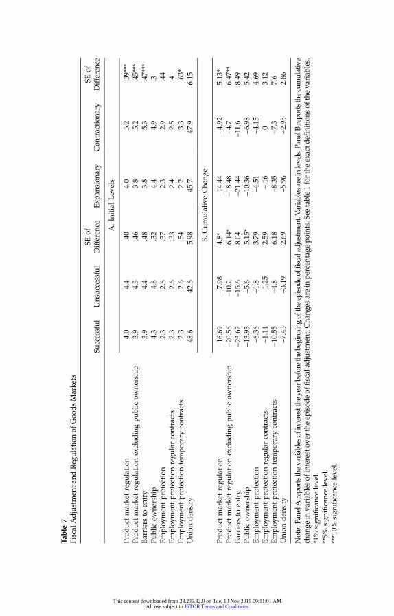
Table

7Fiscal

Adjustmen

tan

dReg

ulationof

Goo

dsMarke

ts

Successful

Unsuc

cessful

SEof

Differen

ceExp

ansion

ary

Con

traction

ary

SEof

Differen

ce

A.Initial

Lev

els

Prod

uctmarke

tregu

lation

4.0

4.4

.40

4.0

5.2

.39***

Prod

uctmarke

tregu

lation

exclud

ingpu

blic

owne

rship

3.9

4.3

.46

3.8

5.2

.45***

Barriersto

entry

3.9

4.4

.48

3.8

5.3

.47***

Public

owne

rship

4.3

4.6

.32

4.4

4.9

.3Employ

men

tprotection

2.3

2.6

.37

2.3

2.9

.44

Employ

men

tprotection

regu

larcontracts

2.3

2.6

.33

2.4

2.5

.4Employ

men

tprotection

tempo

rary

contracts

2.3

2.6

.54

2.2

3.3

.63*

Union

den

sity

48.6

42.6

5.98

45.7

47.9

6.15

B.C

umulativeCha

nge

Prod

uctmarke

tregu

lation

−16.69

−7.98

4.8*

−14.44

−4.92

5.13

*Prod

uctmarke

tregu

lation

exclud

ingpu

blic

owne

rship

−20.56

−10.2

6.14

*−1

8.48

−4.7

6.47

**Barriersto

entry

−23.62

−15.6

8.04

−21.44

−11.6

8.49

Public

owne

rship

−13.93

−5.6

5.15

*−1

0.36

−6.98

5.42

Employ

men

tprotection

−6.36

−1.8

3.79

−4.51

−4.15

4.69

Employ

men

tprotection

regu

larcontracts

−1.14

1.25

2.59

−.16

03.12

Employ

men

tprotection

tempo

rary

contracts

−10.55

−4.8

6.18

−8.35

−7.3

7.6

Union

den

sity

−7.43

−3.19

2.69

−5.96

−2.95

2.86

Note:Pa

nelA

repo

rtsthe

variableso

finterestthe

year

beforethebeginn

ingof

theepisod

eoffiscaladjustm

ent.Variables

areinlevels.Pan

elBrepo

rtsthe

cumulative

chan

gein

variab

lesof

interestov

ertheep

isod

eof

fiscal

adjustmen

t.Cha

nges

arein

percen

tage

points.S


efinitions

oftheva

riab

les.

*1%

sign

ifican

celeve

l.**5%

sign

ifican

celeve

l.***10%

sign

ifican

celeve

l.



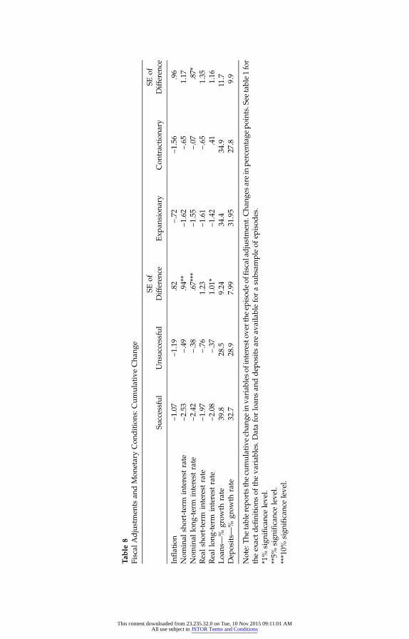
Table

8Fiscal

Adjustmen

tsan

dMon

etaryCon

ditions:C

umulativeCha

nge

Successful

Unsuc

cessful

SEof

Differen

ceExp

ansion

ary

Con

traction

ary

SEof

Differen

ce

Inflation

−1.07

−1.19

.82

−.72

−1.56

.96

Nom

inal

short-term

interest

rate

−2.53

−.49

.94**

−1.62

−.65

1.17

Nom

inal

long

-term

interest

rate

−2.42

−.38

.67***

−1.55

−.07

.87*

Realshort-term

interest

rate

−1.97

−.76

1.23

−1.61

−.65

1.35

Reallong

-term

interest

rate

−2.08

−.37

1.01

*−1

.42

.41

1.16

Loa

ns—

%grow

thrate

39.8

28.5

9.24

34.4

34.9

11.7

Dep

osits—

%grow

thrate

32.7

28.9

7.99

31.95

27.8

9.9

Note:The

tablerepo

rtsthecu

mulativech

ange

inva

riab

lesof

interestov

ertheep

isod

eof

fiscalad

justmen

t.Cha

nges

arein

percen

tage

points.See

table1for

theexactdefinitions

oftheva

riab

les.Dataforloan

san

ddep

ositsareav

ailableforasu

bsam

pleof

episod

es.

*1%

sign

ifican

celeve

l.**5%

sign

ifican

celeve

l.***10%

sign

ifican

celeve

l.



with an increase in confidence. In fact, table 9 shows an increase in con-


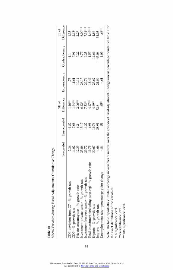
fidence during expansionary and successful adjustments. Whether it isan improvement in economic conditions that improves confidence orthe other way around remains to be seen (see Alesina et al. 2012). Thereduction in nominal interest rates may also be the result of monetaryeasing, which could be endogenous to the fiscal adjustment. If the mon-etary authority perceives a credible policy package of fiscal consolida-tion, it might be more likely to “ease.” The importance of interest ratemovements is highlighted in table 10, which reports a breakdown ofthe various components of GDP. This table shows that all componentsof GDP increased during successful and expansionary adjustments rela-tive to unsuccessful and contractionary ones. However, the effect seemsespecially strong on private investments, which aremore likely to be sen-sitive to interest rates. This result is in line with Alesina et al. (2002, 2012).An additional interesting observation also in line with Alesina andArdagna (1998), Alesina et al. (1998), and Perotti (2013) is that net exportimproves during expansionary and successful adjustments. We now ex-amine competitiveness and exchange rate movements.

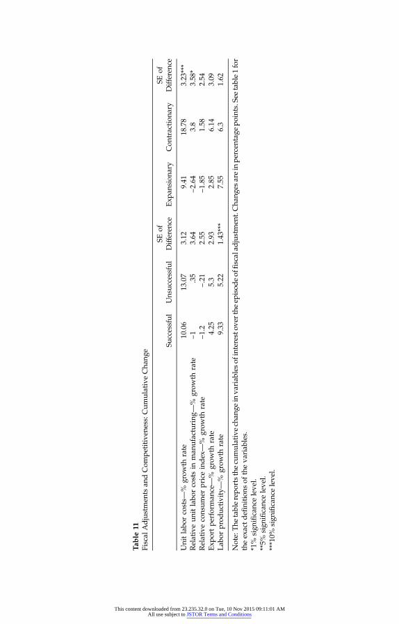
3. Unit Labor Costs and Competitiveness

Table 11 reports results on unit labor costs and competitiveness. The firstrow shows that during successful and expansionary adjustments, unitlabor costs have grown less than during unsuccessful and contractionaryones. Line 2 shows that the same holds not only in absolute terms butrelative to trading partners. Finally, line 3 shows results along the sameline with respect to productivity. This evidence is consistent with thatof labor and goods market deregulation presented above. It shows thatsupply-side reforms and possibly wage moderation and agreementswith the unions (see also Perotti [2013] on this point) have facilitatedthe fiscal adjustment. In other words, the negative Keynesian effect onthe demand side of spending cuts has been overturned with the help ofsupply-side reforms.

4. The Exchange Rate

A few authors (Lambertini and Tavares 2005; IMF 2010; Devries et al.2011) have argued that devaluations have been an important factor inexplaining the success of fiscal adjustments; namely, those that were expan-sionary were so because they were accompanied by large and permanent



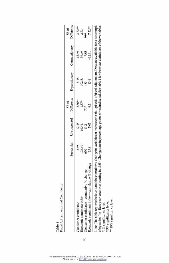
Table

9Fiscal

Adjustmen

tsan

dCon

fiden

ce

Successful

Unsuc

cessful

SEof

Differen

ceExp

ansion

ary

Con

traction

ary

SEof

Differen

ce

Con

sumer

confiden

ce−2

.69

−12.48

2.50

***

−5.48

−15.69

3.82

***

Econo

mic

sentim

entindex

103.64

100.44

1.57

**10

2.51

99.69

2.33

Con

sumer

confiden

ce—

cumulative%

chan

ge67

0−1

1.2

707

483

−7.85

989

Econo

mic

sentim

entindex—

cumulative%

chan

ge13

.85.05

6.3

13.4

−12.91

7.32

***

Note:The

tablerepo

rtsthe

leve

lsan

dthecu

mulativech

ange

inva

riab

leso

finteresto

verthe

episod

eof

fiscalad

justmen

t.Dataareav

ailablefora

subsam

ple

ofep

isod

es(i.e.,Europ

eancoun

triesstarting

in1985).Cha

nges

arein

percen

tage

pointswhe

nindicated

.See

table1forthe

exactd

efinitions

oftheva

riab

les.

*1%

sign

ifican

celeve

l.**5%

sign

ifican

celeve

l.***10%

sign

ifican

celeve

l.

40



Table

10Macro

Variables

duringFiscal

Adjustmen

ts:C

umulativeCha

nge

Successful

Unsuc

cessful

SEof

Differen

ceExp

ansion

ary

Con

traction

ary

SEof

Differen

ce

GDPdev

iation

from

G7—

%grow

thrate

2.36

−1.82

1.16

***

.73

−1.1

1.33

GDP—

%grow

thrate

14.02

7.08

1.94

***

11.61

7.91

2.18

*Privateconsum

ption—

%grow

thrate

12.35

6.2

2.06

***

10.11

7.22

2.27

Inve

stmen

tprivatesector—

%grow

thrate

25.06

13.17

6.42

*26

.17

6.77

6.00

***

Inve

stmen

tbu

sine

sssector—

%grow

thrate

29.72

14.22

7.53

**29

.74

9.25

7.31

***

Totalinve

stmen

t(inc

ludingho

using)—

%grow

thrate

19.75

6.98

4.47

***

18.49

1.57

4.49

***

Exp

orts—

%grow

thrate

30.67

19.76

4.69

**27

.62

19.69

4.89

Impo

rts—

%grow

thrate

−4.66

−38.91

32.6

−21.04

−43.06

34.03

Une

mploy

men

trate—pe

rcen

tage

pointch

ange

−.84

.51

.65**

−.61

1.09

.66**

Note:The

tablerepo

rtsthecu

mulativech

ange

inva

riab

lesof

interestov

ertheep

isod

eof

fiscalad

justmen

t.Cha

nges

arein

percen

tage

points.See

table1for

theexactdefinitions

oftheva

riab

les.

*1%

sign

ifican

celeve

l.**5%

sign

ifican

celeve

l.***10%

sign

ifican

celeve

l.

41



Table

11Fiscal

Adjustmen

tsan

dCom

petitive

ness:C

umulativeCha

nge

Successful

Unsuc

cessful

SEof

Differen

ceExp

ansion

ary

Con

traction

ary

SEof

Differen

ce

Unitlabo

rcosts—

%grow

thrate

10.06

13.07

3.12

9.41

18.78

3.23

***

Relativeun

itlabo

rcostsin

man

ufacturing

—%

grow

thrate

−1.35

3.64

−2.64

3.8

3.58

*Relativeconsum

erpriceindex—

%grow

thrate

−1.2

−.21

2.55

−1.85

1.58

2.54

Exp

ortpe

rforman

ce—

%grow

thrate

4.25

5.3

2.93

2.85

6.14

3.09

Lab

orprod

uctivity—%

grow

thrate

9.33

5.22

1.43

***

7.55

6.3

1.62

Note:The

tablerepo

rtsthecu

mulativech

ange

inva

riab

lesof

interestov

ertheep

isod

eof

fiscalad

justmen

t.Cha

nges

arein

percen

tage

points.See

table1for

theexactdefinitions

oftheva

riab

les.

*1%

sign

ifican

celeve

l.**5%

sign

ifican

celeve

l.***10%

sign

ifican

celeve

l.



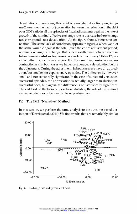
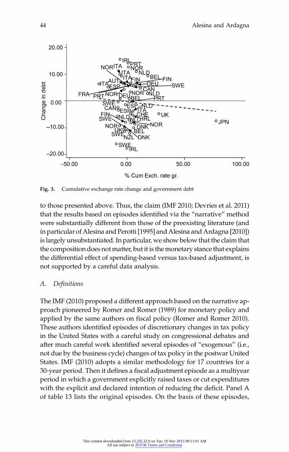
devaluations. In our view, this point is overstated. As a first pass, in fig-


ure 2 we show the (lack of) correlation between the reduction in the debtover GDP ratio in all the episodes of fiscal adjustments against the rate ofgrowth of the nominal effective exchange rate (a decrease in the exchangerate corresponds to a devaluation). As the figure shows, there is no cor-relation. The same lack of correlation appears in figure 3 when we plotthe same variable against the total (over the entire adjustment period)nominal exchange rate change. But is there a difference between success-ful and unsuccessful and expansionary and contractionary? Table 12 pro-vides rather inconclusive answers. For the case of expansionary versuscontractionary, in both cases we have, on average, a devaluation beforethe adjustment. During the adjustment, in both cases we have an appreci-ation, but smaller, for expansionary episodes. The difference is, however,small and not statistically significant. In the case of successful versus un-successful episodes, the appreciation is actually larger than during un-successful ones, but, again, the difference is not statistically significant.Thus, at least on the basis of these basic statistics, the role of the nominalexchange rate does not appear to be so predominant.

IV. The IMF “Narrative” Method

In this section, we perform the same analysis to the outcome-based def-inition of Devries et al. (2011).We find results that are remarkably similar

Fig. 2. Exchange rate and government debt




that the results based on episodes identified via the “narrative” methodwere substantially different from those of the preexisting literature (andinparticularofAlesina andPerotti [1995] andAlesina andArdagna [2010])is largely unsubstantiated. In particular,we showbelow that the claim thatthe compositiondoes notmatter, but it is themonetary stance that explainsthe differential effect of spending-based versus tax-based adjustment, isnot supported by a careful data analysis.

A. Definitions

The IMF (2010) proposed a different approach based on the narrative ap-proach pioneered by Romer and Romer (1989) for monetary policy andapplied by the same authors on fiscal policy (Romer and Romer 2010).These authors identified episodes of discretionary changes in tax policyin the United States with a careful study on congressional debates andafter much careful work identified several episodes of “exogenous” (i.e.,not due by the business cycle) changes of tax policy in the postwar UnitedStates. IMF (2010) adopts a similar methodology for 17 countries for a30-year period. Then it defines a fiscal adjustment episode as a multiyearperiod in which a government explicitly raised taxes or cut expenditureswith the explicit and declared intention of reducing the deficit. Panel Aof table 13 lists the original episodes. On the basis of these episodes,

to those presented above. Thus, the claim (IMF 2010; Devries et al. 2011)

Fig. 3. Cumulative exchange rate change and government debt



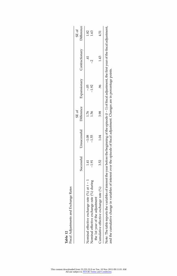
Table

12Fiscal

Adjustmen

tsan

dExcha

ngeRates

Successful

Unsuc

cessful

SEof

Differen

ceExp

ansion

ary

Con

traction

ary

SEof

Differen

ce

Nom

inal

effectiveexch

ange

rate

(%)at

t−1

1.41

−1.08

1.76

−.05

.41

1.82

Nom

inal

effectiveexch

ange

rate

(%)during

the1stye

arof

thead

justmen

t−1

.91

−1.55

1.56

−1.92

−21.63

Cum

ulativeeffectiveexch

ange

rate

(%)

3.52

1.04

3.98

.96

1.43

4.51

Note:The

tablerepo

rtstheva

riab

lesof

interesttheye

arbe

fore

thebe

ginn

ingof

theep

isod

e(t−1)

offiscalad

justmen

t,thefirsty

earo

fthe

fiscalad

justmen

t,an

dthecu

mulativech

ange

inva

riab

lesof

interest

over

theep

isod

eof

fiscal

adjustmen

t.Cha

nges

arein

percen

tage

points.



Table 13Episodes of Fiscal Adjustments

Australia


ments weremore recessionary than spending-based ones, (2) on average,spending-based fiscal adjustmentswere (mildly) recessionary, and (3) thepolicy package mattered. Subsequently Devries et al. (2011) provideda different classification of episodes, which is also reported in panel B

Country Years

Th

A. IMF (2010)

Belgium 1
1980 1985 1986 1987 1994 1995 1996 1997 1998 1999982 1983 1984 1987 1990 1992 1993 1994 1995 1996 1997 1998
Canada 1
980 1981 1982 1983 1984 1985 1986 1987 1988 1989 1990 1991 19921993 1994 1995 1996 1997 1998 1999
Denmark 1
983 1984 1985 1986 1995 Finland 1 984 1988 1992 1993 1994 1996 1997 1998 1999 2000 2006 2007
1984 1986 1987 1988 1989 1991 1995 1996 1997 1998 2000 2006 2007
FranceGermany 1 982 1983 1984 1985 1986 1987 1988 1989 1992 1993 1994 1995 1996
1997 1998 1999 2000 2003 2004 2005 2006 2007
Ireland 1 982 1983 1984 1985 1986 1987 1988 2009 Italy 1 992 1993 1994 1995 1996 1997 1998 2004 2005 2006 2007
1981 1982 1983 1986 1997 2003 2004 2005 2006 2007
JapanPortugal 1 983 2000 2002 2003 2005 2006 2007 Spain 1 983 1984 1985 1986 1987 1988 1989 1992 1993 1994 1995 1996 1997 1998 Sweden 1 983 1984 1986 1992 1993 1994 1995 1996 1997 1998 2007 United Kingdom 1 981 1982 1994 1995 1996 1997 1998 1999 United States 1 980 1981 1985 1986 1988 1990 1991 1993 1994 2000
B. Devries et al. (2011)

Australia 1Austria 1

985 1986 1987 1988 1994 1995 1996 1997 1998 1999980 1981 1984 1996 1997 2001 2002

Belgium 1Canada 1

982 1983 1984 1985 1987 1990 1992 1993 1994 1996 1997984 1985 1986 1987 1988 1989 1990 19911992 1993 1994 1995 1996 1997

Denmark 1
983 1984 1985 1986 1995 Finland 1 992 1993 1994 1995 1996 1997 France 1 979 1987 1989 1991 1992 1995 1996 1997 1999 2000 Germany 1 982 1983 1984 1991 1992 1993 1994 1995 1997 1998 1999 2000 2003
2004 2006 2007
Ireland 1 982 1983 1984 1985 1986 1987 1988 2009 Italy 1 991 1992 1993 1994 1995 1996 1997 1998 2004 2005 2006 2007
1979 1980 1981 1982 1983 1997 1998 2003 2004 2005 2006 2007
JapanNetherlands 1 981 1982 1983 1984 1985 1986 1987 1988 1991 1992 1993 2004 2005 Portugal 1 983 2000 2002 2003 2005 2006 2007 Spain 1 983 1984 1989 1990 1992 1993 1994 1995 1996 1997 Sweden 1 984 1993 1994 1995 1996 1997 1998 United Kingdom 1 979 1980 1981 1982 1994 1995 1996 1997 1998 1999 United States 1 978 1980 1981 1985 1986 1988 1990 1991 1992 1993 1994 1995 1996
1997 1998

IMF (2010) reported essentially three results: (1) tax-based fiscal adjust-

is content downloaded from 23.235.32.0 on Tue, 10 Nov 2015 09:11:01 AMAll use subject to JSTOR Terms and Conditions


of table 13. In what follows we use the episodes of Devries et al. (2011)


rather than IMF (2010) since the former are the corrected “final” list ofepisodes.

B. The Composition of the Adjustments

Table 14 shows that the key result regarding the composition of fiscaladjustments holds using the Devries et al. (2011) dates as well. The suc-cessful and expansionary fiscal adjustments are those that were pri-marily on the current spending side. Also using these episodes, Alesinaet al. (2012) show how different the effects of spending-based and tax-based adjustments were. The former were associated with virtually norecessions, on average, while the latter were accompanied by a prolongeddownturn.Tables 15–21 reproduce the same analysis we had performed above on

the basis of our definition of episodes using the IMF classification. Thebasic result is that exactly the same picture emerges regarding the effectof accompanying policies that lead to expansionary versus contraction-ary episodes. In particular, table 15 shows that there is not a clear patternabout the initial conditions that differentiate the four types of fiscal ad-justments. Table 16 shows that, as discussed above, expansionary fiscaladjustments are more likely to occur in less regulated economies. Table 17shows that expansionary fiscal adjustments are more likely to occur whenthey are accompanied by liberalizations. Table 18 shows that there is nodifference in measures of monetary conditions regarding expansionaryversus contractionary episodes while “easier” monetary conditions seemto have helped adjustments to be successful by lowering interest rates.Table 19 shows positive effects on confidence of expansionary adjustments:once again causality is an issue here. Is confidence driving the expansionsor the otherway around?Amuchmore sophisticated analysis, beyond thescope of this paper, would be necessary to answer this question. Table 20confirms the important role of investment increases during successful fis-cal adjustments, again the same result we obtained above with our defini-tion of adjustment. Table 21 confirms the role of unit labor costs, which fellmuch more on average for expansionary fiscal adjustments than for con-tractionary ones.The bottom line then is that the basic results of the paper—namely, that

(1) spending-based adjustments are much less contractionary or even ex-pansionary than tax-based ones and (2) differences in supply-side policiessuch as liberalization andwagemoderation are key elements of the policymix—are robust to alternative definitions of episodes. They hold for both



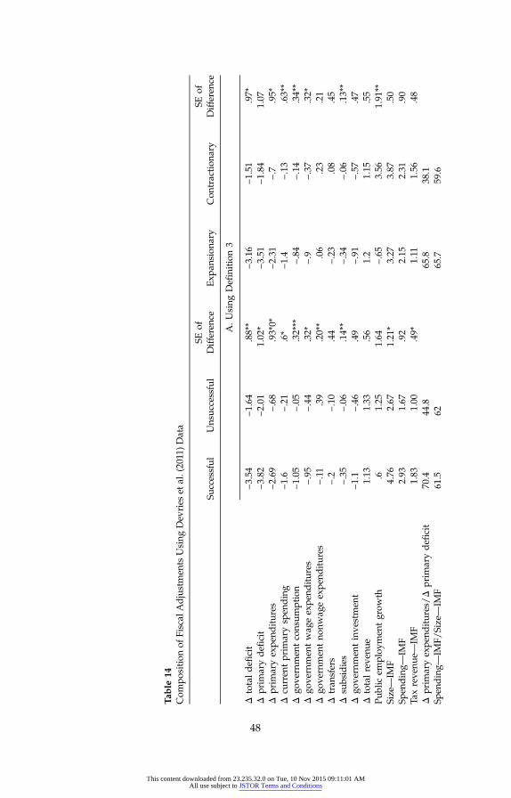
Table

14Com

position

ofFiscal

Adjustmen

tsUsing

Dev

ries

etal.(2011)D

ata

Successful

Unsuc

cessful

SEof

Differen

ceExp

ansion

ary

Con

traction

ary

SEof

Differen

ce

A.U

sing

Definition3

Δtotaldeficit

−3.54

−1.64

.88**

−3.16

−1.51

.97*

Δprim

arydeficit

−3.82

−2.01

1.02

*−3

.51

−1.84

1.07

Δprim

aryexpe

nditures

−2.69

−.68

.93*0*

−2.31

−.7

.95*

Δcu

rren

tprim

arysp

ending

−1.6

−.21

.6*

−1.4

−.13

.63**

Δgo

vernmen

tconsum

ption

−1.05

−.05

.32***

−.84

−.14

.34**

Δgo

vernmen

twag

eexpe

nditures

−.95

−.44

.32*

−.9

−.37

.32*

Δgo

vernmen

tno

nwag

eexpe

nditures

−.11

.39

.20**

.06

.23

.21

Δtran

sfers

−.2

−.10

.44

−.23

.08

.45

Δsu

bsidies

−.35

−.06

.14**

−.34

−.06

.13**

Δgo

vernmen

tinve

stmen

t−1

.1−.46

.49

−.91

−.57

.47

Δtotalreve

nue

1.13

1.33

.56

1.2

1.15

.55

Public

employ

men

tgrow

th.6

1.25

1.64

−.65

3.56

1.91

**Size—IM

F4.76

2.67

1.21

*3.27

3.87

.50

Spen

ding—

IMF

2.93

1.67

.92

2.15

2.31

.90

Taxreve

nue—

IMF

1.83

1.00

.49*

1.11

1.56

.48

Δprim

aryexpe

nditures/Δ

prim

arydeficit

70.4

44.8

65.8

38.1

Spen

ding—

IMF/

Size—

IMF

61.5

6265

.759

.6

48



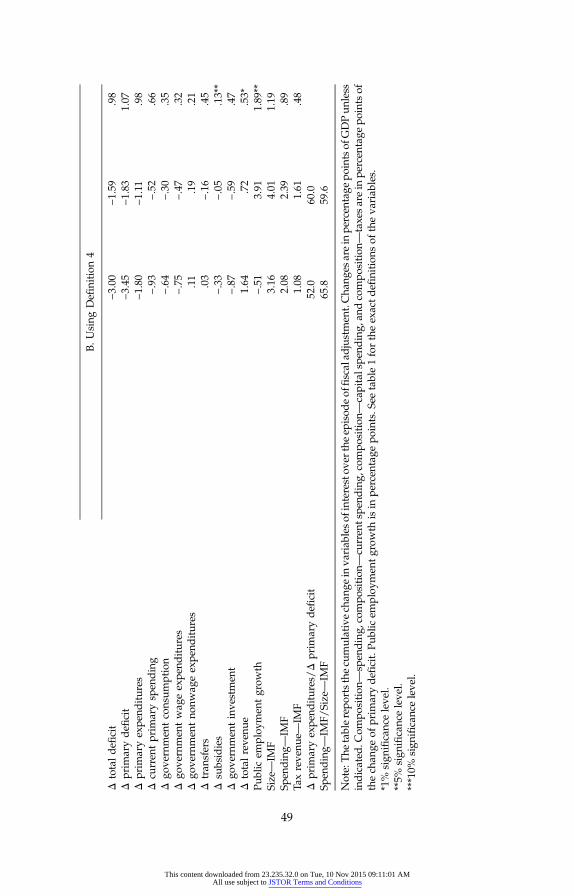
B.U

sing

Definition4

Δtotaldeficit

−3.00

−1.59

.98

Δprim

arydeficit

−3.45

−1.83

1.07

Δprim

aryexpe

nditures

−1.80

−1.11

.98

Δcu

rren

tprim

arysp

ending

−.93

−.52

.66

Δgo

vernmen

tconsum

ption

−.64

−.30

.35

Δgo

vernmen

twag

eexpe

nditures

−.75

−.47

.32

Δgo

vernmen

tno

nwag

eexpe

nditures

.11

.19

.21

Δtran

sfers

.03

−.16

.45

Δsu

bsidies

−.33

−.05

.13**

Δgo

vernmen

tinve

stmen

t−.87

−.59

.47

Δtotalreve

nue

1.64

.72

.53*

Public

employ

men

tgrow

th−.51

3.91

1.89

**Size—IM

F3.16

4.01

1.19

Spen

ding—

IMF

2.08

2.39

.89

Taxreve

nue—

IMF

1.08

1.61

.48

Δprim

aryexpe

nditures/Δ

prim

arydeficit

52.0

60.0

Spen

ding—

IMF/

Size—

IMF

65.8

59.6

Note:The

tablerepo

rtsthecu

mulativech

ange

inva

riab

lesof

interestov

ertheep

isod

eof

fiscalad

justmen

t.Cha

nges

arein

percen

tage

pointsof

GDPun

less

indicated

.Com

position

—sp

ending,

compo

sition

—cu

rren

tspe

nding,

compo

sition

—capitalspe

nding,

andcompo

sition

—taxesarein

percen

tage

pointsof

thech

ange

ofprim

arydeficit.P

ublic

employ

men

tgrowth

isin

percen

tage

points.S


efinitions

oftheva

riab

les.

*1%

sign

ifican

celeve

l.**5%

sign

ifican

celeve

l.***10%

sign

ifican

celeve

l.

49



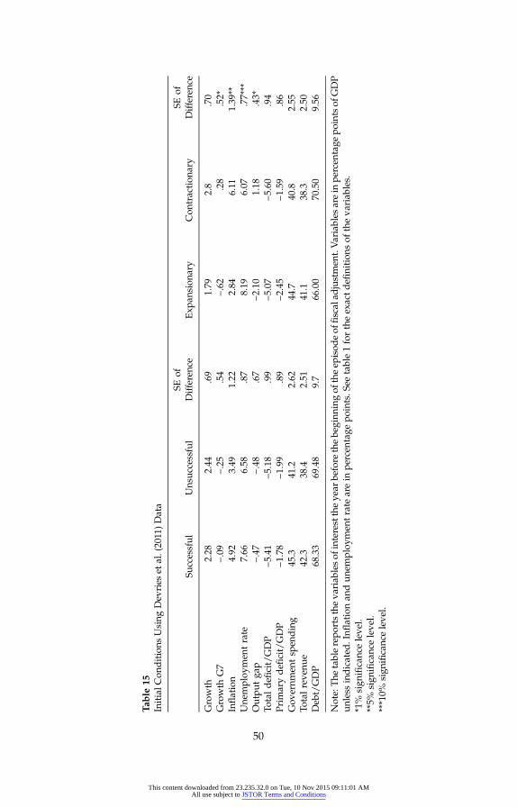
Table

15InitialC

onditions

Using

Dev

ries

etal.(2011)D

ata

Successful

Unsuc

cessful

SEof

Differen

ceExp

ansion

ary

Con

traction

ary

SEof

Differen

ce

Growth

2.28

2.44

.69

1.79

2.8

.70

Growth

G7

−.09

−.25

.54

−.62

.28

.52*

Inflation

4.92

3.49

1.22

2.84

6.11

1.39

**Une

mploy

men

trate

7.66

6.58

.87

8.19

6.07

.77***

Outpu

tga

p−.47

−.48

.67

−2.10

1.18

.43*

Totaldeficit/GDP

−5.41

−5.18

.99

−5.07

−5.60

.94

Prim

arydeficit/GDP

−1.78

−1.99

.89

−2.45

−1.59

.86

Gov

ernm

entsp

ending

45.3

41.2

2.62

44.7

40.8

2.55

Totalreve

nue

42.3

38.4

2.51

41.1

38.3

2.50

Deb

t/GDP

68.33

69.48

9.7

66.00

70.50

9.56

Note:The

tablerepo

rtstheva

riab

lesof

interesttheye

arbe

fore

thebe

ginn

ingof

theep

isod

eof

fiscalad

justmen

t.Variables

arein

percen

tage

pointsof

GDP

unless

indicated

.Inflation

andun

employ

men

tratearein

percen

tage

points.S


efinitions

oftheva

riab

les.

*1%

sign

ifican

celeve

l.**5%

sign

ifican

celeve

l.***10%

sign

ifican

celeve

l.

50



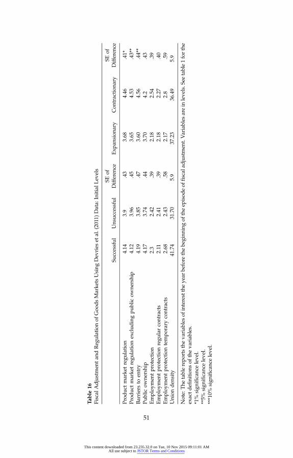
Table

16Fiscal

Adjustmen

tan

dReg

ulationof

Goo

dsMarke

tsUsing

Dev

ries

etal.(2011)D

ata:

InitialL

evels

Successful

Unsuc

cessful

SEof

Differen

ceExp

ansion

ary

Con

traction

ary

SEof

Differen

ce

Prod

uctmarke

tregu

lation

4.14

3.9

.43

3.68

4.46

.41*

Prod

uctmarke

tregu

lation

exclud

ingpu

blic

owne

rship

4.12

3.96

.45

3.65

4.53

.43**

Barriersto

entry

4.19

3.85

.47

3.60

4.56

.44**

Public

owne

rship

4.17

3.74

.44

3.70

4.2

.43

Employ

men

tprotection

2.3

2.42

.39

2.18

2.54

.39

Employ

men

tprotection

regu

larcontracts

2.11

2.41

.39

2.18

2.27

.40

Employ

men

tprotection

tempo

rary

contracts

2.68

2.43

.58

2.17

2.8

.59

Union

den

sity

41.74

31.70

5.9

37.23

36.49

5.9

Note:

The

tablerepo

rtstheva

riab

lesof

interesttheye

arbe

fore

thebe

ginn

ingof

theep

isod

eof

fiscal

adjustmen

t.Variables

arein

leve

ls.S

eetable1forthe

exactd

efinitions

oftheva

riab

les.

*1%

sign

ifican

celeve

l.**5%

sign

ifican

celeve

l.***10%

sign

ifican

celeve

l.

51



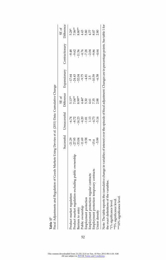
Table

17Fiscal

Adjustmen

tsan

dReg

ulationof

Goo

dsMarke

tsUsing

Dev

ries

etal.(2011)D

ata:

Cum

ulativeCha

nge

Successful

Unsuc

cessful

SEof

Differen

ceExp

ansion

ary

Con

traction

ary

SEof

Differen

ce

Prod

uctmarke

tregu

lation

−21.29

−6.74

5.13

**−1

7.64

−8.48

5.28

*Prod

uctmarke

tregu

lation

exclud

ingpu

blic

owne

rship

−27.95

−8.72

7.04

**−2

4.43

−9.62

7.06

**Barriersto

entry

−33.04

−14.23

8.99

**−3

2.04

−11.56

8.80

**Pu

blic

owne

rship

−11.69

−4.20

4.44

*−9

.75

−4.76

4.43

Employ

men

tprotection

−9.58

−1.81

5.30

−4.81

−7.28

5.80

Employ

men

tprotection

regu

larcontracts

.41.13

4.61

2.5

−2.04

4.77

Employ

men

tprotection

tempo

rary

contracts

−15.6

−4.73

7.35

−10.59

−9.86

8.07

Union

den

sity

−5.99

−5.16

2.88

−6.58

−4.64

2.80

Note:The

tablerepo

rtsthecu

mulativech

ange

inva

riab

lesof

interestov

ertheep

isod

eof

fiscalad

justmen

t.Cha

nges

arein

percen

tage

points.See

table1for

theexactdefinitions

oftheva

riab

les.

*1%

sign

ifican

celeve

l.**5%

sign

ifican

celeve

l.***10%

sign

ifican

celeve

l.

52



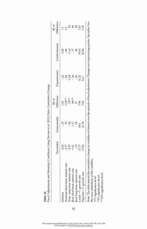
Table

18Fiscal

Adjustmen

tsan

dMon

etaryCon

ditions

Using

Dev

ries

etal.(2011)D

ata:

Cum

ulativeCha

nge

Successful

Unsuc

cessful

SEof

Differen

ceExp

ansion

ary

Con

traction

ary

SEof

Differen

ce

Inflation

−2.03

−.35

1.02

−.22

−1.82

1.1

Nom

inal

short-term

interest

rate

−2.77

.35

1.04

***

−.86

−.86

1.1

Nom

.lon

g-term

interest

rate

−2.57

−.06

.70***

−1.04

−1.14

.79

Realshort-term

interest

rate

−1.61

1.17

.84***

−.26

.17

.96

Reallong

-term

interest

rate

−.73

.76

.9*

−.45

.46

.84

Loa

ns—

%grow

thrate

17.77

18.0

7.98

11.32

19.63

7.67

Dep

osits—

%grow

thrate

17.02

21.76

7.56

14.7

20.84

7.55

Note:The

tablerepo

rtsthecu

mulativech

ange

inva

riab

lesof

interestov

ertheep

isod

eof

fiscalad

justmen

t.Cha

nges

arein

percen

tage

points.See

table1for

theexactdefinitions

oftheva

riab

les.

*1%

sign

ifican

celeve

l.**5%

sign

ifican

celeve

l.***10%

sign

ifican

celeve

l.

53



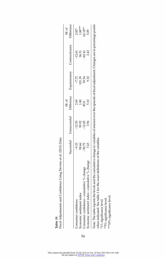
Table

19Fiscal

Adjustmen

tsan

dCon

fiden

ceUsing

Dev

ries

etal.(2011)D

ata

Successful

Unsuc

cessful

SEof

Differen

ceExp

ansion

ary

Con

traction

ary

SEof

Differen

ce

Con

sumer

confiden

ce−9

.33

−12.55

2.69

−7.72

−12.61

2.82

*Econo

mic

sentim

entindex

98.66

99.92

1.80

101.39

96.51

1.80

***

Con

sumer

confiden

ce—

cumulative%

chan

ge−5

0.75

−12.85

85.8

59.54

−82.41

62.18**

Econo

mic

sentim

entindex—

cumulative%

chan

ge7.63

3.96

5.10

9.32

2.43

5.09

Note:The

tablerepo

rtstheleve

lsan

dthecu

mulativech

ange

inva

riab

lesof

interestov

ertheep

isod

eof

fiscalad

justmen

t.Cha

nges

arein

percen

tage

points

whe

nindicated

.See

table1fortheexactd

efinitions

oftheva

riab

les.

*1%

sign

ifican

celeve

l.**5%

sign

ifican

celeve

l.***10%

sign

ifican

celeve

l.

54



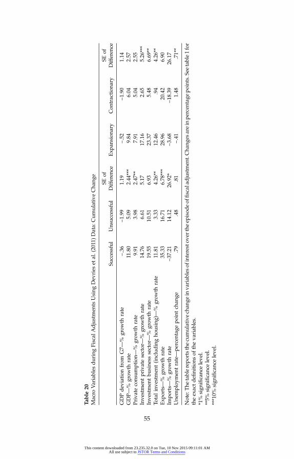
Table

20Macro

Variables

duringFiscal

Adjustmen

tsUsing

Dev

ries

etal.(2011)D

ata:

Cum

ulativeCha

nge

Successful

Unsuc

cessful

SEof

Differen

ceExp

ansion

ary

Con

traction

ary

SEof

Differen

ce

GDPdev

iation

from

G7—

%grow

thrate

−.36

−1.99

1.19

−.52

−1.90

1.14

GDP—

%grow

thrate

11.80

5.09

2.44

***

9.84

6.04

2.57

Privateconsum

ption—

%grow

thrate

9.91

3.98

2.47

**7.91

5.04

2.55

Inve

stmen

tprivatesector—

%grow

thrate

14.76

6.61

5.17

17.16

2.65

5.26

***

Inve

stmen

tbu

sine

sssector—

%grow

thrate

19.55

10.51

6.93

23.37

5.48

6.69

**To

talinve

stmen

t(inc

ludingho

using)—

%grow

thrate

11.81

3.33

4.26

**12

.46

.94

4.26

**Exp

orts—

%grow

thrate

35.33

16.71

6.78

***

28.96

20.42

6.90

Impo

rts—

%grow

thrate

−37.21

14.12

26.92*

−3.68

−18.39

26.17

Une

mploy

men

trate—pe

rcen

tage

pointch

ange

.79

.48

.81

−.41

1.48

.71**

Note:The

tablerepo

rtsthecu

mulativech

ange

inva

riab

lesof

interestov

ertheep

isod

eof

fiscalad

justmen

t.Cha

nges

arein

percen

tage

points.See

table1for

theexactdefinitions

oftheva

riab

les.

*1%

sign

ifican

celeve

l.**5%

sign

ifican

celeve

l.***10%

sign

ifican

celeve

l.

55



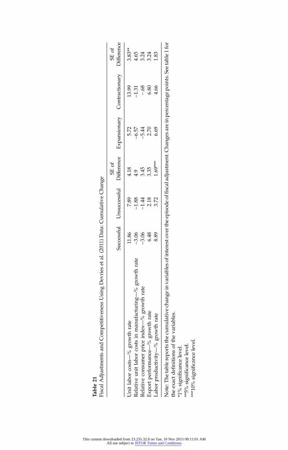
Table

21Fiscal

Adjustmen

tsan

dCom

petitive

ness

Using

Dev

ries

etal.(2011)D

ata:

Cum

ulativeCha

nge

Successful

Unsuc

cessful

SEof

Differen

ceExp

ansion

ary

Con

traction

ary

SEof

Differen

ce

Unitlabo

rcosts—

%grow

thrate

11.86

7.89

4.18

5.72

13.99

3.83

**Relativeun

itlabo

rcostsin

man

ufacturing

—%

grow

thrate

−3.06

−1.88

4.9

−6.57

−1.31

4.65

Relativeconsum

erpriceindex—

%grow

thrate

−3.06

−1.44

3.45

−5.44

−.68

3.24

Exp

ortpe

rforman

ce—

%grow

thrate

6.48

2.18

3.35

2.70

6.80

3.24

Lab

orprod

uctivity—%

grow

thrate

8.89

3.72

1.69

***

6.69

4.66

1.83

Note:The

tablerepo

rtsthecu

mulativech

ange

inva

riab

lesof

interestov

ertheep

isod

eof

fiscalad

justmen

t.Cha

nges

arein

percen

tage

points.See

table1for

theexactdefinitions

oftheva

riab

les.

*1%

sign

ifican

celeve

l.**5%

sign

ifican

celeve

l.***10%

sign

ifican

celeve

l.



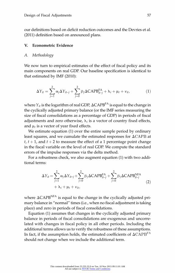
our definitions based on deficit reduction outcomes and the Devries et al.


(2011) definition based on announced plans.

V. Econometric Evidence

A. Methodology

We now turn to empirical estimates of the effect of fiscal policy and itsmain components on real GDP. Our baseline specification is identical tothat estimated by IMF (2010):

ΔYit ¼X2

j¼1

αjΔYit−j þX2

j¼0

βjΔCAPBFAit−j þ λi þ μt þ νit; ð1Þ

whereYit is the logarithm of real GDP,ΔCAPBFA is equal to the change inthe cyclically adjusted primary balance (or the IMF series measuring thesize of fiscal consolidations as a percentage of GDP) in periods of fiscaladjustments and zero otherwise, λi is a vector of country fixed effects,and μt is a vector of year fixed effects.We estimate equation (1) over the entire sample period by ordinary

least squares, and we cumulate the estimated responses for ΔCAPB att, tþ 1, and tþ 2 to measure the effect of a 1 percentage point changein the fiscal variable on the level of real GDP. We compute the standarderrors of the impulse responses via the delta method.For a robustness check, we also augment equation (1) with two addi-

tional terms:

ΔYit ¼X2

j¼1

αjΔYit−jþX2

j¼0

βjΔCAPBFAit−j þ

X2

j¼0

βjΔCAPBNFAit−j

ð2Þþ λi þ μt þ νit;

where ΔCAPBNFA is equal to the change in the cyclically adjusted pri-mary balance in “normal” times (i.e., when no fiscal adjustment is takingplace) and zero in periods of fiscal consolidations.Equation (1) assumes that changes in the cyclically adjusted primary

balance in periods of fiscal consolidations are exogenous and uncorre-lated with changes in fiscal policy in all other periods. Including theadditional terms allows us to verify the robustness of these assumptions.In fact, if the assumption holds, the estimated coefficients of ΔCAPBFA

should not change when we include the additional term.



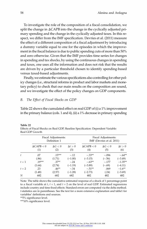
To investigate the role of the composition of a fiscal consolidation, we


split the change in ΔCAPB into the change in the cyclically adjusted pri-mary spending and the change in the cyclically adjusted taxes. In this re-spect, we differ from the IMF specification. Devries et al. (2011) measurethe effect of a different composition of a fiscal adjustment by introducinga dummy variable equal to one for the episodes in which the improve-ment in the fiscal balance is due to public spending cuts ofmore than 50%and zero otherwise. Given that the IMF provides time series for changesin spending and tax shocks, by using the continuous changes in spendingand taxes, one uses all the information and does not risk that the resultsare driven by a particular threshold chosen to identify spending-basedversus taxed-based adjustments.Finally,weestimate thevarious specifications also controlling forotherpol-

icy changes (i.e., structural reforms in product and labor markets andmone-tary policy) to check that our main results on the composition are sound,and we investigate the effect of the policy changes on GDP components.

B. The Effect of Fiscal Shocks on GDP

Table 22 shows the cumulated effect on realGDP of (i) a 1% improvementin the primary balance (cols. 1 and 4), (ii) a 1%decrease in primary spending

Table 22Effects of Fiscal Shocks on Real GDP, Baseline Specification: Dependent Variable:
Real GDP Growth
Fiscal Adjustments:Definition 1

Fiscal Adjustments:IMF (Devries et al. 2011)

Thesca

ΔCAPB < 0(1)

ΔG < 0(2)

Δt > 0(3)

the ve e res, tþ þ 2 lev

This content downloaded from 23.235.32.0 on TuAll use subject to JSTOR Terms a

ΔCAPB < 0(4)

ΔG < 0(5)

Δt > 0(6)

t
.07(.86)
.15***(1.71)

−.12(−1.00)

−.33**(−3.15)

ck. E

e, 10 Nov 2015 09:11:01nd Conditions

−.096(−.56)

ntareg

AM

−.64**(−3.49)

tþ 1
.19***(1.64)
.37**(2.74)

−.24(−1.19)

−.63**(−3.89)

−.177(−.69)

−1.35**(−4.11)

.23
.46** −.34 −.51** .069 −1.6** tþ 2 (1.48) (2.57) (−1.28) (−2.73) (.24) (−3.69) 682 682 682 482 482 482 N
Note:
table shows cumulati stimated ponse of a sho of 1 perce ge point to a fi l variable at t 1, and t on the el of real GDP stimated ressions include country and time fixed effects. Standard errors are computed via the delta method.t-statistics are in parentheses. See the text for a more extensive explanation and table1 forvariables’ definitions and sources.**5% significance level.***10% significance level.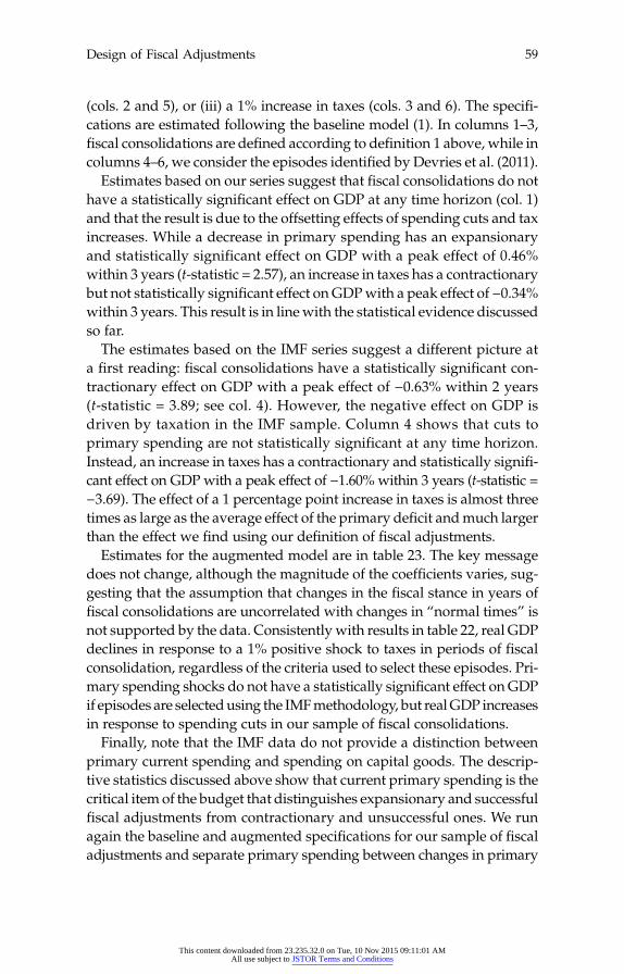

(cols. 2 and 5), or (iii) a 1% increase in taxes (cols. 3 and 6). The specifi-


cations are estimated following the baseline model (1). In columns 1–3,fiscal consolidations are defined according to definition 1 above, while incolumns 4–6, we consider the episodes identified by Devries et al. (2011).Estimates based on our series suggest that fiscal consolidations do not

have a statistically significant effect on GDP at any time horizon (col. 1)and that the result is due to the offsetting effects of spending cuts and taxincreases. While a decrease in primary spending has an expansionaryand statistically significant effect on GDP with a peak effect of 0.46%within 3 years (t-statistic = 2.57), an increase in taxes has a contractionarybut not statistically significant effect onGDPwith a peak effect of −0.34%within 3 years. This result is in linewith the statistical evidence discussedso far.The estimates based on the IMF series suggest a different picture at

a first reading: fiscal consolidations have a statistically significant con-tractionary effect on GDP with a peak effect of −0.63% within 2 years(t-statistic = 3.89; see col. 4). However, the negative effect on GDP isdriven by taxation in the IMF sample. Column 4 shows that cuts toprimary spending are not statistically significant at any time horizon.Instead, an increase in taxes has a contractionary and statistically signifi-cant effect on GDP with a peak effect of −1.60% within 3 years (t-statistic =−3.69). The effect of a 1 percentage point increase in taxes is almost threetimes as large as the average effect of the primary deficit andmuch largerthan the effect we find using our definition of fiscal adjustments.Estimates for the augmented model are in table 23. The key message

does not change, although the magnitude of the coefficients varies, sug-gesting that the assumption that changes in the fiscal stance in years offiscal consolidations are uncorrelated with changes in “normal times” isnot supported by the data. Consistently with results in table 22, real GDPdeclines in response to a 1% positive shock to taxes in periods of fiscalconsolidation, regardless of the criteria used to select these episodes. Pri-mary spending shocks do not have a statistically significant effect onGDPif episodes are selectedusing the IMFmethodology, but realGDP increasesin response to spending cuts in our sample of fiscal consolidations.Finally, note that the IMF data do not provide a distinction between

primary current spending and spending on capital goods. The descrip-tive statistics discussed above show that current primary spending is thecritical item of the budget that distinguishes expansionary and successfulfiscal adjustments from contractionary and unsuccessful ones. We runagain the baseline and augmented specifications for our sample of fiscaladjustments and separate primary spending between changes in primary



Table 23Effects of Fiscal Shocks on Real GDP, Augmented Specification: Dependent Variable:

Th the ve esp ck o ntasca t, t tþ vel Es reg


We find that shocks to the former have a statistically significant effect onGDP but not to the latter. Moreover, the effect on GDP of a decrease incurrent primary spending is even larger than the effect of a decrease in

Table 24

Real GDP Growth

Fiscal Adjustments:Definition 1

Fiscal Adjustments:IMF (Devries et al. 2011)

Effects o

Thle

ΔCAPB < 0(1)

ΔG < 0(2)

Δt > 0(3)

f Primary Spending Components on Real G

la onth P.

This content downloaded from 23.235.32.0 on TueAll use subject to JSTOR Terms an

ΔCAPB < 0(4)

ΔG < 0(5)

Δt > 0(6)

t
.06(.79)
.15****(1.74)

−.17(−1.43)

−.36**(−3.51)

DP: Dependent V

, 10 Nov 2015 09:11:01 Ad Conditions

−.08(−.49)

ariable:

tanc

M

−.72**(−4.08)

tþ 1
.18(1.49)
.32**(2.44)

−.33****(−1.70)

−.68**(−4.25)

−.19(−.77)

−1.51**(−4.82)

.19
.38** −.41 −.55** .01 −1.81** tþ 2 (1.28) (2.23) (−1.60) (−2.96) (.06) (−4.35) 682 682 682 482 482 482 N
Note:
e table shows cumulati estimated r onse of a sho f 1 perce ge point to a fi l variable at þ 1, and 2 on the le of real GDP. timated ressions
current spending and spending on capital goods. Results are in table 24.

include country and time fixed effects. Standard errors are computed via the delta method.t-statistics are in parentheses. See the text for a more extensive explanation and table 1 forvariables’ definitions and sources.**5% significance level.***10% significance level.

Real GDP Growth

Fiscal Adjustments:Definition 1 Baseline Specifications

Fiscal Adjustments:Definition 1 Augmented Specifications

Δ Primary CurrentSpending < 0

Δ GovernmentInvestment < 0

Δ Primary CurrentSpending < 0

Δ GovernmentInvestment < 0

t
.29**(2.38)
−.06(−.42)

.3**(2.55)

−.09(−.68)

tþ 1
.63**(3.52)
−.08(−.32)

.53**(3.09)

−.17(−.67)

.73**
−.07 .62** −.19 tþ 2 (3.07) (−.22) (2.74) (−.55) 682 682 682 682 N
Note:
e table shows the cumu tive estimated resp seof a shockof 1percen gepoint toa fiscal variab at t, tþ 1, and tþ 2 on e level of real GD Estimated regressions i lude country and time fixed effects. Standard errors are computedvia the deltamethod. t-statistics are inparentheses.See the text for a more extensive explanation and table 1 for variables’ definitions and sources.**5% significance level.

total primary spending. A reduction of 1 percentage point of GDP in cur-


rent primary spending has a peak effect of 0.73% (t-statistic = 3.07)within3 years compared with a 0.46% effect due to a reduction in total primaryspending by the same magnitude.

C. Monetary Policy

Wenow investigatewhether the results on the effect of spending cuts andtax increases hold when we control for changes in monetary or exchangerate policies. First, we study the effect of spending and tax changes on themonetary policy variables. Second, we add among the right-hand side ofequations (1) and (2) the short-term nominal interest rates or the changein the nominal effective exchange rate. Results are in tables 25 and 26.Whenwe identify episodes of fiscal adjustments using definition 1, we

find that the short-term interest rate increases in response to tax increasesbut falls when spending is cut. However, these effects are not statisticallysignificant. Instead, when we consider the IMF episodes, we find evi-dence that monetary policy reacts differently to the spending and taxchanges as the short-term interest rate increases in response to tax hikesand falls in response to spending cuts and coefficients are statistically sig-nificant. This suggests that monetary policy might endogenously re-spond to the type of the adjustments and central banks might decide

Table 25
Effects of Fiscal Shocks on Short-Term Interest Rates
Baseline Specification Augmented Specification

Ts

FiscalAdjustments:

FiscalAdjustments: IMF

s e e es rl 2 o e

This content downloaded from 23.235.32.0 on All use subject to JSTOR Term

FiscalAdjustments:


t

Definition 1

ΔG < 0 Δt > 0

(Devries et al. 2011)

ΔG < 0 Δt > 0

Definition 1

ΔG < 0 Δt > 0

fs

Tue, 10 Nov 2015 09:11:01 As and Conditions


ΔG < 0 Δt > 0

−.1(−1.23)

.15(1.31)

−.18(−1.11)

.53**(2.71)

−.11(−1.43)

.15(1.25)

−.26(−1.58)

ntagregr

M

.55**(2.88)

tþ 1
−.11(−.72)
.29(1.22)

−.51***(−1.74)

.8***(1.88)

−.11(−.74)

.31(1.30)

−.58**(−2.0)

.88**(2.14)

−.13
.37 −.86** .81 −.14 .39 −.9** .95 tþ 2 (−.60) (1.04) (−2.29) (1.27) (−.63) (1.13) (−2.44) (1.53)
Note:
he table hows th cumulativ timated esponse o a shock of 1 perce e point to a fi cal variab e at t, tþ 1, and tþ n short-t rm intere t rates. E stimated essions include country and time fixed effects. Standard errors are computed via the delta method.t-statistics are in parentheses. See the text for a more extensive explanation and table 1 forvariables’ definitions and sources.**5% significance level.***10% significance level.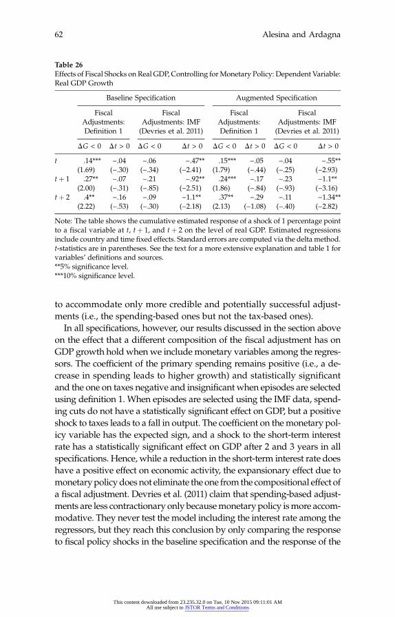

to accommodate only more credible and potentially successful adjust-

Table 26Effects of Fiscal Shocks on Real GDP, Controlling forMonetary Policy: Dependent Variable:

T s e ive o entas b t tþ l a E reg


ments (i.e., the spending-based ones but not the tax-based ones).In all specifications, however, our results discussed in the section above

on the effect that a different composition of the fiscal adjustment has onGDP growth hold when we include monetary variables among the regres-sors. The coefficient of the primary spending remains positive (i.e., a de-crease in spending leads to higher growth) and statistically significantand the one on taxes negative and insignificant when episodes are selectedusing definition 1. When episodes are selected using the IMF data, spend-ing cuts do not have a statistically significant effect on GDP, but a positiveshock to taxes leads to a fall in output. The coefficient on themonetary pol-icy variable has the expected sign, and a shock to the short-term interestrate has a statistically significant effect on GDP after 2 and 3 years in allspecifications. Hence, while a reduction in the short-term interest rate doeshave a positive effect on economic activity, the expansionary effect due tomonetarypolicy does not eliminate the one from the compositional effect ofa fiscal adjustment. Devries et al. (2011) claim that spending-based adjust-ments are less contractionary only becausemonetarypolicy ismore accom-modative. They never test the model including the interest rate among theregressors, but they reach this conclusion by only comparing the responseto fiscal policy shocks in the baseline specification and the response of the

Real GDP Growth


FiscalAdjustments:


This content downloaded from 23.235.32.0 onAll use subject to JSTOR Term

FiscalAdjustments:


t

Definition 1

ΔG < 0 Δt > 0


ΔG < 0 Δt > 0

Definition 1

ΔG < 0 Δt > 0

Tue, 10 Nov 2015 09:11:01s and Conditions


ΔG < 0 Δt > 0

.14***(1.69)

−.04(−.30)

−.06(−.34)

−.47**(−2.41)

.15***(1.79)

−.05(−.44)

−.04(−.25)

AM

−.55**(−2.93)

tþ 1
.27**(2.00)
−.07(−.31)

−.21(−.85)

−.92**(−2.51)

.24***(1.86)

−.17(−.84)

−.23(−.93)

−1.1**(−3.16)

.4**
−.16 −.09 −1.1** .37** −.29 −.11 −1.34** tþ 2 (2.22) (−.53) (−.30) (−2.18) (2.13) (−1.08) (−.40) (−2.82)
Note:
he table hows th cumulat estimated response f a shock of 1 perc ge point to a fi cal varia le at t, þ 1, and 2 on the evel of re l GDP. stimated ressions include country and time fixed effects. Standard errors are computed via the delta method.t-statistics are in parentheses. See the text for a more extensive explanation and table 1 forvariables’ definitions and sources.**5% significance level.***10% significance level.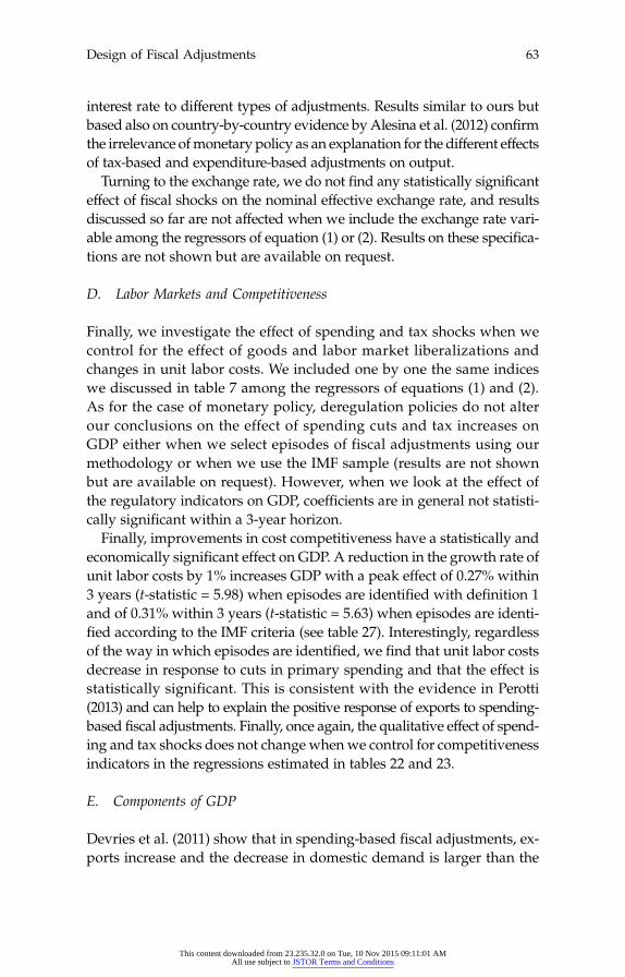

interest rate to different types of adjustments. Results similar to ours but


based also on country-by-country evidence byAlesina et al. (2012) confirmthe irrelevance ofmonetary policy as an explanation for the different effectsof tax-based and expenditure-based adjustments on output.Turning to the exchange rate, we do not find any statistically significant

effect of fiscal shocks on the nominal effective exchange rate, and resultsdiscussed so far are not affected when we include the exchange rate vari-able among the regressors of equation (1) or (2). Results on these specifica-tions are not shown but are available on request.

D. Labor Markets and Competitiveness

Finally, we investigate the effect of spending and tax shocks when wecontrol for the effect of goods and labor market liberalizations andchanges in unit labor costs. We included one by one the same indiceswe discussed in table 7 among the regressors of equations (1) and (2).As for the case of monetary policy, deregulation policies do not alterour conclusions on the effect of spending cuts and tax increases onGDP either when we select episodes of fiscal adjustments using ourmethodology or when we use the IMF sample (results are not shownbut are available on request). However, when we look at the effect ofthe regulatory indicators on GDP, coefficients are in general not statisti-cally significant within a 3-year horizon.Finally, improvements in cost competitiveness have a statistically and

economically significant effect on GDP. A reduction in the growth rate ofunit labor costs by 1% increases GDP with a peak effect of 0.27% within3 years (t-statistic = 5.98) when episodes are identified with definition 1and of 0.31% within 3 years (t-statistic = 5.63) when episodes are identi-fied according to the IMF criteria (see table 27). Interestingly, regardlessof the way in which episodes are identified, we find that unit labor costsdecrease in response to cuts in primary spending and that the effect isstatistically significant. This is consistent with the evidence in Perotti(2013) and can help to explain the positive response of exports to spending-based fiscal adjustments. Finally, once again, the qualitative effect of spend-ing and tax shocks does not change whenwe control for competitivenessindicators in the regressions estimated in tables 22 and 23.

E. Components of GDP

Devries et al. (2011) show that in spending-based fiscal adjustments, ex-ports increase and the decrease in domestic demand is larger than the



total effect onGDP. They attribute the positive response of exports to a dif-

Table 27Effects of Fiscal Shocks on Unit Labor Costs: Dependent Variable % Δ Unit Labor Costs

e es o ntag2 o a . ns i


ferent behavior of the exchange rate. Also, they do not estimate the effecton private consumption and investment but on total domestic demand,including public spending and inventories. We investigated the effect ofa reduction in primary spending (increases in taxes) on private consump-tion, business investment, and exports separately.Our results, available onrequest, are very much in line with those in tables 22 and 23. When epi-sodes are selected using definition 1, spending cuts (tax increases) havea positive (negative) effect on private consumption, business and privateinvestment, and exports. When episodes are selected using the IMF defi-nition, reductions in public spending have a negative and significant effectonly on private consumption after 1 year. The effect on private consump-tion is not statistically significant 2 and 3 years after the adjustment.Instead, spending cuts have a positive and statistically significant effectboth on exports (after 1 and 3 years) and on business investment (3 yearsafter the consolidation). Tax increases are always recessionary.

VI. Conclusions

In the last 2 years there has been a very lively debate about what are theconsequences of different types of fiscal adjustments. In this paper we


FiscalAdjustments:


This content downloaded from 23.235.32.0 oAll use subject to JSTOR Ter

FiscalAdjustments:


t

Definition 1

ΔG < 0 Δt > 0


ΔG < 0 Δt > 0

Definition 1

ΔG < 0 Δt > 0

n Tue, 10 Nov 2015 09:11:01 Ams and Conditions


ΔG < 0 Δt > 0

−.27**(−2.02)

.39**(2.04)

−.64**(−2.59)

.33(1.20)

−.33**(−2.50)

.4**(2.22)

−.64**(−2.76)

M

.35(1.37)

tþ 1
−.43**(−1.92)
.57****(1.68)

−1.07**(−2.79)

.57(1.12)

−.48**(−2.23)

.56****(1.77)

−.99**(−2.74)

.59(1.23)

−.37
.75 −1.47** .52 −.47 .68 −1.28** .45 tþ 2 (−1.22) (1.63) (−3.35) (.76) (−1.61) (1.55) (−3.10) (.70)
Note:
The table shows the cumulativ timated response f a shock of 1 perce e point to a fi scal variab le at t, tþ 1, and tþ n unit l bor costs Estimated regressio nclude country and time fixed effects. Standard errors are computed via the deltamethod. t-statisticsare in parentheses. See the text for a more extensive explanation and table 1 for variables’definitions and sources.**5% significance level.***10% significance level.

have taken a detailed look at recent controversies and performed a host


of sensitivity tests, changing definitions and exploring alternative ap-proaches. We also have brought into the picture other variables such asgoods and labor market liberalizations, which sometimes accompanyfiscal adjustments.Our results can be summarized as follows: expenditure-based adjust-

ments are those that are more likely to lead to a permanent reductionin the debt over GDP ratio. In addition, they are associated with smallerrecessions than tax-based ones or no recessions at all. The component ofprivate demand that seems to react more positively to an expenditure-based adjustment is private investment. Cuts in current spending havea smaller or no effect on output than cuts in public investments. The smalldownturns caused by expenditure-based adjustments can be eliminated,making the adjustment expansionary even on impact, if the policy pack-age includes progrowth policies such as labor and goods market liber-alization. Monetary policy has the standard effect on output, but it doesnot seem to play a role in differentiating the effects of tax-based versusexpenditure-based adjustments.

Endnotes

We thank Jeff Brown, Carlo Cottarelli, Carlo Favero, Francesco Giavazzi, Paolo Mauro,and participants in the 2012American Economic Association session on Fiscal Adjustmentsand the 2012 Tax Policy and the Economy conference for useful comments and GiampaoloLecce and Andrea Passalacqua for excellent research assistantship. Views and conclusionsexpressed in this paper are those of the authors and do not necessarily represent those ofGoldman Sachs. The authors alone are responsible for any remaining errors. For acknowl-edgments, sources of research support, and disclosure of the authors’ material financialrelationships, if any, please see http://www.nber.org/chapters/c12853.ack.

1. An incomplete list includes IMF (1996), McDermott and Wescott (1996), Alesina,Perotti, and Tavares (1998), vonHagen and Strauch (2001), and Broadbent and Daly (2010).

2. See Nielsen (2012) for an analysis of current fiscal consolidation programs ongoing inEurope.

3. These are the countries that were members of the OECD group for the entire sampleperiod. We exclude Luxembourg.

4. Alesina and Ardagna (2010) define a period of fiscal adjustment as a year in which thecyclically adjusted primary balance improves by at least 1.5% of GDP. Alesina and Perotti(1995) defined a period of fiscal adjustment as a year in which the cyclically adjusted pri-mary balance improves by at least 2% of GDP per year or a period of consecutive years inwhich the cyclically adjusted primary balance improves by at least 1% of GDP per year. Thequalitative nature of the results did not change, and conclusions were also robust tochanges in the threshold chosen.

5. See Stehn et al. (2011) for evidence on the nonlinear effect on the speed of fiscal tight-ening and the possibility that fiscal consolidations that are too large induce a large contrac-tion in economic activity and undermine the deficit reduction.

6. An important point for future research relates to long-run unfunded liabilities of gov-ernments such as social security funds. To what extent do “major policy changes” includefixing the long-term trend of certain programs, such as Medicare in the United States?



References


Alesina, A., and S. Ardagna. 1998. “Tales of Fiscal Adjustment.” Economic Policy13, no. 27:487–545.

———. 2010. “Large Changes in Fiscal Policy: Taxes versus Spending.” TaxPolicy and the Economy 24:35–68.

Alesina, A., S. Ardagna, R. Perotti, and F. Schiantarelli. 2002. “Fiscal PolicyProfits and Investment.” American Economic Review 92, no. 3:571–89.

Alesina, A., C. Favero, and F. Giavazzi. 2012. “The Output Effects of FiscalAdjustments.” Working Paper no 18336, NBER, Cambridge, MA.

Alesina, A., and F. Giavazzi, eds. 2013. Fiscal Policy after the Financial Crisis.Chicago: University of Chicago Press (for NBER).

Alesina, A., and R. Perotti. 1995. “Fiscal Expansions and Adjustments in OECDCountries.” Economic Policy 21:207–47.

Alesina, A., R. Perotti, and J. Tavares. 1998. “The Political Economy of FiscalAdjustments.” Brookings Papers on Economic Activity, no. 1:197–248.

Ardagna, S. 2004. “Fiscal Stabilizations: When Do They Work and Why?”European Economic Review 48, no. 5:1047–74.

———. 2007. “Fiscal Policy in Unionized Labor Markets.” Journal of EconomicDynamics and Control 31:1498–1534.

Biggs, A., K. Hasset, and M. Jensen. 2010. “A Guide for Deficit Reduction in theUnited States Based on Historical Consolidations That Worked.” EconomicPolicy Working Paper no. 2010-04 (December 27), American Enterprise Insti-tute, Washington, DC.

Blanchard, O. 1993. “Suggestions for a New Set of Fiscal Indicators.” In ThePolitical Economy of Government Debt, ed. H. A. A. Verbon and F. A. A. M.Winden, 307–25. Amsterdam: North-Holland.

Broadbent, B., and K. Daly. 2010. “Limiting the Fall-out from Fiscal Adjust-ment.” Global Economics Paper no. 195 (April), Goldman Sachs, New York.

Daveri, F., and G. Tabellini. 2000. “Unemployment Growth and Taxation inIndustrial Countries.” Economic Policy 15:47–104.

Devries, P., J. Guajardo, D. Leigh, and A. Pescatori. 2011. “A New Action-BasedDataset of Fiscal Consolidation.” Working Paper no. 11/128, InternationalMonetary Fund, Washington, DC. http://www.imf.org/external/pubs/cat/longres.aspx?sk=24892.0.

Favero, C., F. Giavazzi, and J. Perego. 2011. “Country Heterogeneity and theInternational Evidence on the Effects of Fiscal Policy.” IMF Economic Review59:652–82.

Finn, M. 1998. “Cyclical Effects of Government’s Employment and Good Pur-chases.” International Economic Review 39, no. 3:635–57.

Giavazzi, F., and M. Pagano. 1990. “Can Severe Fiscal Contractions Be Expan-sionary? Tales of Two Small European Countries.” NBER MacroeconomicsAnnual 5:75–122.

IMF. 1996. World Economic Outlook. Chapter 3. Washington, DC: InternationalMonetary Fund.

———. 2010. “Will It Hurt? Macroeconomic Effects of Fiscal Consolidation.”In World Economic Outlook: Recovery, Risk, and Rebalancing. Washington, DC:International Monetary Fund.

Lambertini, L., and J. Tavares. 2005. “Exchange Rates and Fiscal Adjustments:Evidence from OECD and Implications for the EMU.” B.E. Journal of Macro-economics: Contributions to Macroeconomics 5, no. 1.



McDermott, J., and R. Wescott. 1996. “An Empirical Analysis of Fiscal Adjust-ments.” IMF Staff Papers 43, no. 4:723–53.


Nielsen, L. 2012. “Who Is Delivering on the Fiscal Front So Far?” EuropeanEconomics Analyst (August).

Perotti, R. 2013. “The ‘Austerity Myth’: Gain without Pain?” In Fiscal Policy afterthe Financial Crisis, ed. A. Alesina and F. Giavazzi. Chicago: University ofChicago Press (for NBER).

Romer, C., and D. Romer. 1989. “Does Monetary Policy Matter? A New Test inthe Spirit of Friedman and Schwartz.” NBER Macroeconomics Annual 4:121–70.

———. 2010. “The Macroeconomic Effects of Tax Changes: Estimates Based ona NewMeasure of Fiscal Shocks.” American Economic Review 100, no. 3:763–801.

Stehn, J., J. Hatzius, D. Wilson, and S. Carlson. 2011. “The Speed Limit ofFiscal Consolidations.” Global Economics Paper no. 207, Goldman Sachs,New York.

von Hagen, J., and R. Strauch. 2001. “Fiscal Consolidations: Quality, EconomicConditions, and Success.” Public Choice 109, nos. 3–4:327–46.





Documents

The Design of Fiscal Adjustments - The National Bureau of ... · 2 The Design of Fiscal Adjustments Alberto Alesina, Harvard University, IGIER, and NBER Silvia Ardagna, Goldman Sachs