The Detection and Exploration of Planets from

the Trans-atlantic Exoplanet Survey

Thesis by

Francis T. O’Donovan

In Partial Fulfillment of the Requirements

for the Degree of

Doctor of Philosophy

California Institute of Technology

Pasadena, California

2008

(Defended July 31, 2007)

ii

c© 2008

Francis T. O’Donovan

All Rights Reserved

iii

For Bridget and Fran, now united with Francis, Jackie, Brıd, James, and Nellie,

For my family of PhDs: Tom, Vera, and Bridget,

For Cathy, a ridiculously lovely human being,

And for all who believed that I could.

iv

Acknowledgements

As those most likely to actually read my entire thesis, I would first like to thank the

faculty who served on my candidacy and defense committees. Thanks to Wal Sargent

and Andrew Blain for stepping in on short notice, to Tony Readhead for understand-

ing the lure of extrasolar planets, to Mike Brown for putting Pluto in its place, and to

Re’em Sari for helping to keep Cathy alive under water! This thesis work could not

have succeeded without Lynne Hillenbrand, who provided all of the benefits of having

two advisors without making me try to please two masters. Finally, I owe a lot to my

advisor David Charbonneau, who first enticed me to the dark side of exoplanets, and

kept my spirits up when the prospects of planet discovery looked bleak. Though he

moved 3,000 miles away to be with his wife—the nerve!—he proved that long-distance

advising can work. (Indeed, I still cringe at the sound of our office phone.)

Strange though it is to acknowledge an inanimate object, without the tireless

workhorse that is Sleuth, I would not have helped discover three planets, which might

have put the brakes on graduating. Despite a lonely existence on Mount Palomar,

Sleuth was very reliable, even when rained on, unless David or I got on a plane!

More importantly, I must thank those at Palomar Observatory, especially Dipali,

Jean, Karl, and Rose, who kept me company on my many one-hour visits. I sincerely

thank Robert Brucato, Michael Doyle, Karl Dunscombe, Richard Ellis, Brian Gordon,

John Henning, Linley Kroll, Steven Kunsman, Jean Mueller, Hal Petrie, Andrew Pick-

les, Nick Scoville, Merle Sweet, Robert Thicksten, Greg van Idsinga, Richard Wetzel,

and Daniel Zieber for their assistance with the fabrication, operation, and mainte-

nance of the Sleuth instrument.

My discoveries with Sleuth would never have happened without the help of the

v

TrES team and collaborators. I have never learned so much about astronomy as

I did at our May meetings. My thanks to Roi Alonso, Gaspar Bakos, Nairn Bal-

iber, Tim Brown, Orlagh Creevey, Jonathan Devor, Ted Dunham, Juan Belmonte,

Hans Deeg, Gil Esquerdo, Mark Everett, Jose Fernandez, Scott Gaudi, Marton Hi-

das, Matt Holman, Luke Kotredes, Geza Kovacs, David Latham, Georgi Mandu-

shev, Markus Rabus, Alex Sozzetti, Bob Stefanik, John Trauger, Willie Torres, Rus-

sel White, and Josh Winn.

Money makes the world go round, and I gratefully acknowledge the financial

support of my thesis work with Sleuth from NASA under the grant NNG05GJ29G,

issued through the Origins of Solar Systems Program.

I wish to recognize and acknowledge the very significant cultural role and rever-

ence that the summit of Mauna Kea has always had within the indigenous Hawaiian

community. I am most fortunate to have the opportunity to conduct observations

from this mountain. Part of this work is based on observations made with the Spitzer

Space Telescope, which is operated by the Jet Propulsion Laboratory, California In-

stitute of Technology under a contract with NASA. This research has made use of the

SIMBAD database, operated at CDS, Strasbourg, France, and NASA’s Astrophysics

Data System Bibliographic Services. This publication also utilizes data products

from the Two Micron All Sky Survey, which is a joint project of the University of

Massachusetts and the Infrared Processing and Analysis Center/California Institute

of Technology, funded by the National Aeronautics and Space Administration and

the National Science Foundation. This research has made use of the USNOFS Image

and Catalogue Archive operated by the United States Naval Observatory, Flagstaff

Station.

My thanks to Alicia, Chao, Luke, Sean, and Joanna, my classmates. You helped

me survive first year—Amigo’s margaritas will never taste as good as they did as I

drank them with my fellow sufferers! And of course Cathy, Elina, Laura, Margaret,

Melissa, Milan and Stuartt, who continued the great tradition of getting to know

the First Years, though some more than others. One’s fellow graduate students are a

tremendous source of advice regarding all aspects of life. My thanks to all the Caltech

vi

Astronomy students that I have known over the years. A special mention must be

made of Micol and Chin for their help choosing the ring, and of Brian and Danielle for

their help choosing our wine! My thanks also to all the Astronomy staff that made my

thesis possible, especially to Patrick Shopbell, Anu Mahabul, and Cheryl Southard

for keeping my computers working!

During my thesis, I visited David Charbonneau quite often at the Harvard–Smith-

sonian Center for Astrophysics. I thank all of the students there for their warm

welcome, in particular Cullen, Heather, Jonathan, Jose, Lisa, and Manuel. I also

thank Blue and her family for giving me a second home away from home.

Surprisingly, I did find time to meet people outside of Caltech. Karen, our Good

Samaritan, has helped me and Cathy through all of our marathon struggles—I’ll take

running the LA marathon over finishing a PhD any day! My quest to complete 26.2

miles of hell was also aided by the presence of the never-say-die Pasadena Pacers.

I treasure my time over the last five years with my extended family, especially the

new additions, and my friends in Cork. Though separated from me by 6,000 miles,

they have continued to be an important part of my life. They have always made time

for me during my visits home, and made me feel like I had never left.

I would never have attempted the PhD program at Caltech without the support of

my parents, Tom and Vera, in particular their relentless faith that I can do anything

that I put my mind to. They have given so much to me that can never be repaid,

and I am proud to call them not only my parents, but two of my best friends. I know

they will always welcome me back in Cork, especially if I fix the computer one more

time!

It’s great having a older sibling. She is always an inspiration, a listener, a friend.

I thank my big sister, my “Best Sister”, Bridget, for always being 18 months older

than me, and for letting her younger brother boss her around sometimes. While I

struggled to complete my thesis, she managed to finish hers while working a full-time

job. She makes it all look easy.

And of course, my loving thanks to Cathy, who has gotten to know the real me

this year. While preparing for her own defense on the same day as mine, she always

vii

kept some energy to bolster me when things got too much for me, and richly deserves

being mentioned three times in these acknowledgments. She knows me so well, the

only time I managed to surprise her was the day I asked her to marry me. Now that

our graduate student days are over, I look forward to a new life together, her hand

in mine.

viii

Abstract

I present the discovery of three transiting planets (TrES-2, TrES-3, and TrES-4) of

nearby bright stars made with the ten-centimeter telescope Sleuth as part of the

Trans-atlantic Exoplanet Survey (TrES). TrES-2 is the first transiting exoplanet de-

tected in the field of view of NASA’s Kepler mission. Of the 20 known transiting

exoplanets, TrES-3 has the second shortest period, facilitating the study of orbital

decay and atmospheric evaporation. Its visible/infrared brightness makes TrES-3 an

ideal target for observations to determine the atmospheric composition. TrES-4 has

the largest radius and lowest density of the known transiting planets. These three

planets have radii larger than that of Jupiter, and the radius of TrES-4 significantly

exceeds predictions from models of hot Jupiters, indicating a possible lack of an energy

source in these models.

I present the results of Spitzer observations of TrES-2. I reject tidal dissipation of

eccentricity as an explanation for the inflated radius, and examine the spectrum for

evidence of atmospheric absorption.

I have monitored 19 fields each containing 6,000–36,000 stars for evidence of tran-

sits. I discuss the rejection of six of my candidate transiting systems from an early

field that represent examples of the 67 astrophysical false positives that I encountered

in Sleuth data. These six false positives highlight the benefit of a multisite survey

such as TrES, and also of comprehensive follow-up of transit candidates. As a fur-

ther example, I present the candidate GSC 03885-00829 from Sleuth data that was

revealed to be a blend of a bright F dwarf and a fainter K-dwarf eclipsing binary.

This candidate proved nontrivial to reject, requiring multicolor follow-up photometry

to produce evidence of the true binary nature of this candidate.

ix

The yield of planets from transit surveys is not yet well constrained or under-

stood. There are numerous factors that affect the predictions such as the amount of

correlated photometric noise present in the data. Here I present an analysis of my

ability to recover fake transits in TrES data. I examined both the automated transit-

search algorithm and my own visual identification process. I find the recovery rate

of my visual analysis to be 87% for those transit candidates that had a sufficiently

high signal-to-noise ratio to be flagged by my transit-search algorithm and readily

identifiable by eye.

x

Contents

Acknowledgements iv

Abstract viii

List of Figures xiii

List of Tables xv

1 Transiting Exoplanets 1

1.1 The Search for Other Worlds Using Starlight . . . . . . . . . . . . . . 1

1.2 Methods for Detecting Hot Jupiters and Other Exoplanets . . . . . . 2

1.2.1 Radial Velocities . . . . . . . . . . . . . . . . . . . . . . . . . 2

1.2.2 Transits . . . . . . . . . . . . . . . . . . . . . . . . . . . . . . 7

1.3 Formation, Structure, and Composition of Highly-Irradiated Gas Giants 10

1.3.1 The Birth of Giants . . . . . . . . . . . . . . . . . . . . . . . . 11

1.3.2 A Core or Not a Core, That is the Question . . . . . . . . . . 11

1.3.3 Extrasolar Atmospheres . . . . . . . . . . . . . . . . . . . . . 13

1.4 Thesis Motivation—Past and Present . . . . . . . . . . . . . . . . . . 14

1.5 Thesis Outline . . . . . . . . . . . . . . . . . . . . . . . . . . . . . . . 15

2 Outcome of Six Candidate Transiting Planets from a TrES Field in

Andromeda 19

Abstract . . . . . . . . . . . . . . . . . . . . . . . . . . . . . . . . . . . . . 19

2.1 Finding a Needle in a Haystack . . . . . . . . . . . . . . . . . . . . . 20

2.2 Follow-up Observations of Planetary Candidates: A Review . . . . . 23

xi

2.3 Initial Observations of a Field in Andromeda . . . . . . . . . . . . . . 28

2.4 Searching for Transit Candidates in Andromeda . . . . . . . . . . . . 28

2.5 Follow-up of Candidate Transiting Planets . . . . . . . . . . . . . . . 34

2.6 Rejecting False-Positive Detections . . . . . . . . . . . . . . . . . . . 38

2.7 Maximizing the Yield from TrES . . . . . . . . . . . . . . . . . . . . 45

3 Rejecting Astrophysical False Positives from the TrES Transiting

Planet Survey: The Example of GSC 03885-00829 47

Abstract . . . . . . . . . . . . . . . . . . . . . . . . . . . . . . . . . . . . . 47

3.1 Transits versus Blended Eclipses . . . . . . . . . . . . . . . . . . . . . 48

3.2 TrES Telescope Observations of

GSC 03885-00829 . . . . . . . . . . . . . . . . . . . . . . . . . . . . . 52

3.3 Spectroscopic Follow-up of GSC 03885-00829 . . . . . . . . . . . . . . 56

3.4 Photometric Follow-up of GSC 03885-00829 . . . . . . . . . . . . . . 59

3.5 Blend Analysis of Observations of

GSC 03885-00829 . . . . . . . . . . . . . . . . . . . . . . . . . . . . . 62

3.6 Confirmation of Blend Model . . . . . . . . . . . . . . . . . . . . . . 66

3.7 The Necessity of Blend Identification . . . . . . . . . . . . . . . . . . 70

4 TrES-2: The First Transiting Planet in the Kepler Field 72

Abstract . . . . . . . . . . . . . . . . . . . . . . . . . . . . . . . . . . . . . 72

4.1 The Search for Transiting Exoplanets . . . . . . . . . . . . . . . . . . 72

4.2 Observations and Analysis of TrES-2 . . . . . . . . . . . . . . . . . . 73

4.3 Estimates of Planet Parameters and Conclusions . . . . . . . . . . . . 81

5 TrES-3: A Nearby, Massive, Transiting Hot Jupiter in a 31-Hour

Orbit 84

Abstract . . . . . . . . . . . . . . . . . . . . . . . . . . . . . . . . . . . . . 84

5.1 Transiting Exoplanets with Very-Short Orbital Periods . . . . . . . . 85

5.2 Observations and Analysis of TrES-3 . . . . . . . . . . . . . . . . . . 86

5.3 Estimates of Planet Parameters and Conclusions . . . . . . . . . . . . 92

xii

6 Detection of Planetary Emission from TrES-2 using Spitzer/IRAC 96

Abstract . . . . . . . . . . . . . . . . . . . . . . . . . . . . . . . . . . . . . 96

6.1 Spitzer Observations of the Known Transiting Exoplanets . . . . . . 97

6.2 IRAC Observations of TrES-2 . . . . . . . . . . . . . . . . . . . . . . 98

6.3 Deriving and Modeling Light Curves of TrES-2 . . . . . . . . . . . . . 99

6.4 Atmospheric Models for TrES-2 . . . . . . . . . . . . . . . . . . . . . 102

6.5 Searching for Evidence of Atmospheric Absorption . . . . . . . . . . . 103

7 Identifying Transits in TrES Data Sets: The Human Factor 105

7.1 Understanding the Yield of Transit Surveys . . . . . . . . . . . . . . 105

7.2 Injecting Model Light Curves into a TrES Data Set . . . . . . . . . . 107

7.3 BLS and Visual-Recovery Methods of Injected Transits . . . . . . . . 120

7.4 BLS and Visual-Recovery Rates . . . . . . . . . . . . . . . . . . . . . 121

7.5 Discussion . . . . . . . . . . . . . . . . . . . . . . . . . . . . . . . . . 134

8 Summary 135

A TrES-4: A Transiting Hot Jupiter of Very-Low Density 137

Abstract . . . . . . . . . . . . . . . . . . . . . . . . . . . . . . . . . . . . . 137

A.1 Understanding the Mass–Radius Relations of Exoplanets . . . . . . . 138

A.2 Photometry and Spectroscopy of TrES-4 . . . . . . . . . . . . . . . . 138

A.3 Properties of TrES-4 and Discussion . . . . . . . . . . . . . . . . . . . 145

B Properties of Known Transiting Systems 148

C The Box-fitting Least-Squares (BLS) Transit-Search Algorithm 151

C.1 A General Description of the BLS Algorithm . . . . . . . . . . . . . . 151

C.2 The Signal Residue and Signal Detection Efficiency . . . . . . . . . . 152

Bibliography 154

xiii

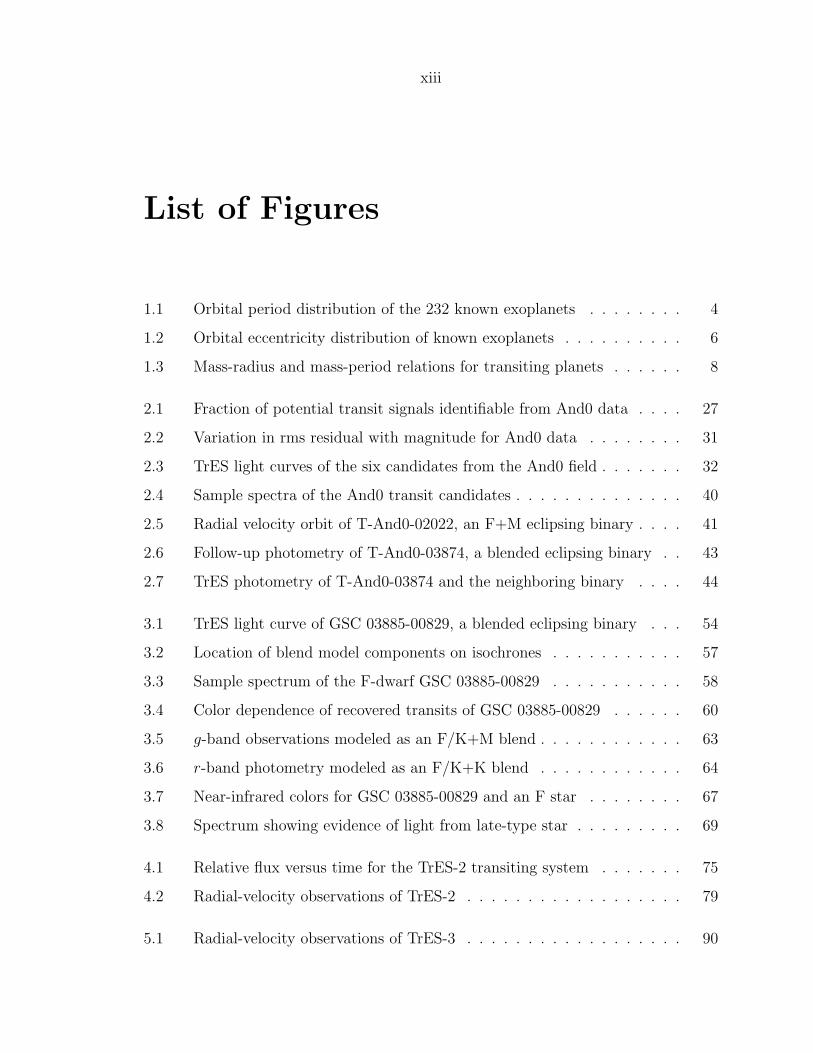
List of Figures

1.1 Orbital period distribution of the 232 known exoplanets . . . . . . . . 4

1.2 Orbital eccentricity distribution of known exoplanets . . . . . . . . . . 6

1.3 Mass-radius and mass-period relations for transiting planets . . . . . . 8

2.1 Fraction of potential transit signals identifiable from And0 data . . . . 27

2.2 Variation in rms residual with magnitude for And0 data . . . . . . . . 31

2.3 TrES light curves of the six candidates from the And0 field . . . . . . . 32

2.4 Sample spectra of the And0 transit candidates . . . . . . . . . . . . . . 40

2.5 Radial velocity orbit of T-And0-02022, an F+M eclipsing binary . . . . 41

2.6 Follow-up photometry of T-And0-03874, a blended eclipsing binary . . 43

2.7 TrES photometry of T-And0-03874 and the neighboring binary . . . . 44

3.1 TrES light curve of GSC 03885-00829, a blended eclipsing binary . . . 54

3.2 Location of blend model components on isochrones . . . . . . . . . . . 57

3.3 Sample spectrum of the F-dwarf GSC 03885-00829 . . . . . . . . . . . 58

3.4 Color dependence of recovered transits of GSC 03885-00829 . . . . . . 60

3.5 g-band observations modeled as an F/K+M blend . . . . . . . . . . . . 63

3.6 r-band photometry modeled as an F/K+K blend . . . . . . . . . . . . 64

3.7 Near-infrared colors for GSC 03885-00829 and an F star . . . . . . . . 67

3.8 Spectrum showing evidence of light from late-type star . . . . . . . . . 69

4.1 Relative flux versus time for the TrES-2 transiting system . . . . . . . 75

4.2 Radial-velocity observations of TrES-2 . . . . . . . . . . . . . . . . . . 79

5.1 Radial-velocity observations of TrES-3 . . . . . . . . . . . . . . . . . . 90

xiv

5.2 Relative flux versus time for the TrES-3 transiting system . . . . . . . 93

6.1 Near-infrared relative fluxes from TrES-2 from Spitzer observations . . 100

6.2 Near-infrared contrast ratios for TrES-2 . . . . . . . . . . . . . . . . . 102

7.1 Histogram of 2MASS J − Ks for TrES Lyr1 field . . . . . . . . . . . . 107

7.2 Randomized stellar parameters for injected transits . . . . . . . . . . . 108

7.3 Randomized planetary parameters for injected transits . . . . . . . . . 109

7.4 Randomized transit impact parameters and orbital inclinations . . . . 111

7.5 Randomized values for first two BLS parameters . . . . . . . . . . . . 113

7.6 Randomized values for final two BLS parameters . . . . . . . . . . . . 114

7.7 Example of model transits . . . . . . . . . . . . . . . . . . . . . . . . . 115

7.8 Example of TrES light curve with injected transits . . . . . . . . . . . 116

7.9 Histograms of BLS SDEs for fake data set . . . . . . . . . . . . . . . . 118

7.10 Example of an injected transit candidate with a high SDE . . . . . . . 119

7.11 SDE and VT versus period for BLS-recovered transits . . . . . . . . . . 122

7.12 Histogram of SDEs for BLS-recovered transit candidates . . . . . . . . 123

7.13 Ratio of ∆ to σ versus period for BLS-recovered transits . . . . . . . . 124

7.14 BLS recovery rates for different orbital periods and planetary radii . . 126

7.15 BLS recovery rates for different stellar radii and impact parameters . . 127

7.16 SDE and VT versus period for visually recovered transits . . . . . . . . 128

7.17 Histogram of SDEs for visually recovered transit candidates . . . . . . 129

7.18 ∆/σ versus period for visually recovered transits . . . . . . . . . . . . 130

7.19 Visual-recovery rates for different periods and planetary radii . . . . . 132

7.20 Visual recovery of different stellar radii and impact parameters . . . . 133

A.1 High-precision follow-up z-band and B-band photometry of TrES-4 . . 142

A.2 Keck/HIRES radial velocity observations of TrES-4 . . . . . . . . . . . 144

xv

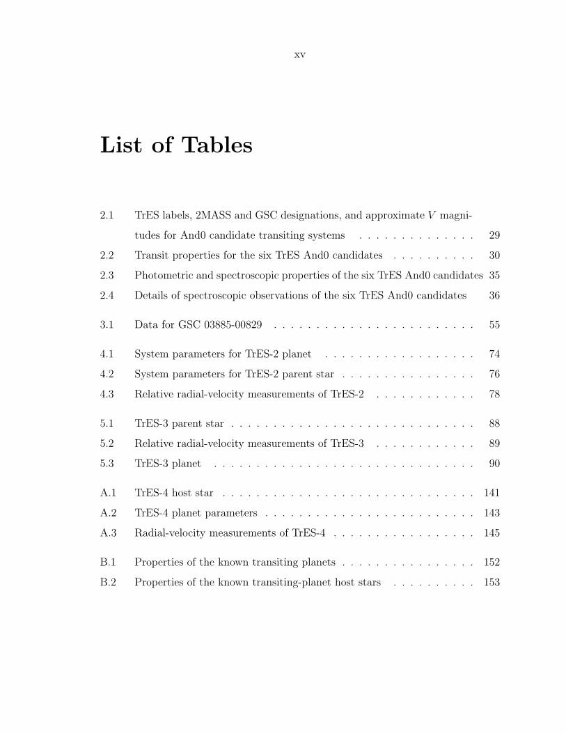
List of Tables

2.1 TrES labels, 2MASS and GSC designations, and approximate V magni-

tudes for And0 candidate transiting systems . . . . . . . . . . . . . . 29

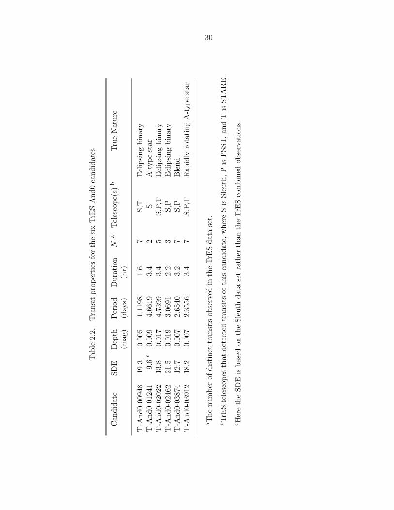
2.2 Transit properties for the six TrES And0 candidates . . . . . . . . . . 30

2.3 Photometric and spectroscopic properties of the six TrES And0 candidates 35

2.4 Details of spectroscopic observations of the six TrES And0 candidates 36

3.1 Data for GSC 03885-00829 . . . . . . . . . . . . . . . . . . . . . . . . 55

4.1 System parameters for TrES-2 planet . . . . . . . . . . . . . . . . . . 74

4.2 System parameters for TrES-2 parent star . . . . . . . . . . . . . . . . 76

4.3 Relative radial-velocity measurements of TrES-2 . . . . . . . . . . . . 78

5.1 TrES-3 parent star . . . . . . . . . . . . . . . . . . . . . . . . . . . . . 88

5.2 Relative radial-velocity measurements of TrES-3 . . . . . . . . . . . . 89

5.3 TrES-3 planet . . . . . . . . . . . . . . . . . . . . . . . . . . . . . . . 90

A.1 TrES-4 host star . . . . . . . . . . . . . . . . . . . . . . . . . . . . . . 141

A.2 TrES-4 planet parameters . . . . . . . . . . . . . . . . . . . . . . . . . 143

A.3 Radial-velocity measurements of TrES-4 . . . . . . . . . . . . . . . . . 145

B.1 Properties of the known transiting planets . . . . . . . . . . . . . . . . 152

B.2 Properties of the known transiting-planet host stars . . . . . . . . . . 153

1

Chapter 1

Transiting Exoplanets

1.1 The Search for Other Worlds Using Starlight

Astronomy in the 21st century has seen significant progress made in the age-old

question of our uniqueness in the universe. Less than two decades since the first

discoveries of planetary-mass systems around stars other than our Sun (Latham et al.,

1989; Wolszczan & Frail, 1992; Mayor & Queloz, 1995), we now know of 200 planetary

systems, and the rate of new discoveries is increasing. The planets in these new

systems are known as “extrasolar planets” or “exoplanets” for short.

Since the reflected or emitted light from a planet is very dim compared with

starlight, the vast majority of detections have been made by studying the light from

the host star as the star interacts with the planet. Software and hardware improve-

ments have made possible the detection of minute changes in observations of these

stars. This thesis work, and the study of exoplanets in general, utilizes telescopes

both on the ground and in space, and ranging from ten-centimeter to ten-meter in

diameter. With these tools, we are able to test our understanding of how gas giants

are formed and how their internal structure and chemical composition vary with en-

vironment. With each new discovery, we make another step toward the detection of

a solar system analog or a mirror Earth in the habitable zone of a star.

Before continuing, it should be noted that a distinction is made—by the Interna-

tional Astronomical Union (IAU), if not by nature—between different types of stellar

companions that are thereby segregated by mass. The evolution of celestial objects

2

that fuse hydrogen in their cores is quite different from the evolution of objects with-

out this fusion. Hence, only the hydrogen-burning bodies (those that have at least

80 times the mass, MJup, of Jupiter) are called stars. Objects that are less massive

than stars, yet can fuse deuterium in their cores, are known as brown dwarfs, and

have masses greater than 13MJup. Finally, the least massive stellar companions are

planets. The latter are the target of my survey, and the planets found during this

thesis work have masses mp ∼ MJup, well below the 13MJup limit, hence different

interpretations of the mass boundaries will not affect my results.

1.2 Methods for Detecting Hot Jupiters and Other

Exoplanets

The majority of the known exoplanetary systems contain planets similar in mass to

Jupiter and the other solar system giant planets, rather than the lighter terrestrial

planets such as Earth. This is because most of the exoplanets were found by measuring

a change in the motion of their star caused by the gravitational presence of the orbiting

planet, a method that is inherently more sensitive to massive planets. The velocity

of a star in space can be split into two components: the radial velocity along the line

of sight to the star (either toward or away from us), and the tangential velocity across

the sky, perpendicular to the line of sight. Although there are several other successful

methods to find exoplanets, in this thesis I will concentrate on a planet search that

uses the measurement of radial-velocity variations to confirm the existence of planets

observed to transit across stellar disks.

1.2.1 Radial Velocities

The radial velocity of a star is determined from the Doppler shifts of the stellar

spectral lines due to the motion of the star. By measuring the variation with time of

the radial velocities of the star (of mass M⋆) and deriving the stellar orbit around the

barycenter of the system, we can determine several orbital parameters of the planet,

3

such as the orbital period P and the eccentricity e. We can also estimate its mass, or

at least a lower limit to the mass, from these orbital parameters and the amplitude

of the variation. The product of the planetary mass mp and the sine of the orbital

inclination i can be computed from the mass function:

(mp sin i)3

(M⋆ + mp)2=

PK3

2πG(1 − e2)3/2,

where K is the semi-amplitude of the radial velocity variation and G is the universal

gravitational constant. This product is known as the minimum mass of the planet.

Assuming a circular orbit and that mp << M⋆, we can write this as:

mp sin i ≃ 1 MJup

(

K

200 m s−1

) (

P

day

)1/3 (

M⋆

M⊙

)2/3

. (1.1)

Thus, the gravitational effect of Jupiter on the Sun is quite small, resulting in a motion

of 12.5 m s−1 or 45 km hr−1, whereas a 1MJup planet in a one-day period around the

sun would induce a motion of K = 200 m s−1. The ability to measure from many

parsecs away these small orbital accelerations requires measuring shifts in the stellar

spectral lines with a precision of roughly one thousandth of the width of a spectral

line. Hardware and software developments have improved this precision to the point

where it is possible to detect planets with minimum masses of ∼5M⊕(∼0.02MJup;

e.g., Gliese 581c; Udry et al., 2007).

Although the radial-velocity surveys are the most prolific planet campaigns, they

suffer from several limitations. The target stars are observed one at a time, requiring

a heavy investment of large telescope time. The surveys are restricted to the brightest

stars in the sky, again due to limited telescope resources. Finally, the precision of

these measurements is not likely to be indefinitely improved, due to an astrophysical

limit. Stars are asteroseismically active, producing radial-velocity “jitter” on the scale

of 1–10 m s−1 (Saar, Butler, & Marcy, 1998; Santos et al., 2000; Wright, 2005). It is

thought that this jitter will hinder achieving precisions much better than currently

obtained.

4

Figure 1.1 Orbital period distribution of the 232 known exoplanets as a functionof their minimum masses. Jupiter is shown for comparison as a red, filled circle.Relatively few massive planets with short orbital periods have been found, despitethe bias for such planets in the radial-velocity surveys. An approximate detectionthreshold (defined as K = 4σ, see text) is shown as a dotted line.

5

The enlarging catalog of planets from radial-velocity surveys of stars in the so-

lar neighborhood facilitates studying the statistics of exoplanets. For example, the

frequency of planets can be estimated from the yield of these surveys, and is cur-

rently estimated at ∼5% for planets of 0.5–8MJup within 3 AU (Udry et al., 2007).

There is a correlation between the metallicity of stars and this frequency of planets

around them (Gonzalez, 1997; Fischer & Valenti, 2003; Santos, Israelian, & Mayor,

2004; see Gonzalez, 2006 for a review). We can also see that known exoplanets

have a wide range in orbital periods, as shown in figure 1.1. This figure also shows

a distinct decreasing trend in the mass of the planet with the short orbital period

(Zucker & Mazeh, 2002; Udry, Mayor, & Santos, 2003), which may be related to the

way in which these gas giants come to be located so close to their stars (see sec-

tion 1.3.1). The lack of low mass planets at longer periods can be explained in terms

of the detection threshold of radial-velocity surveys. Planets can be detected if they

induce a motion K ∼> 4σ in their star, where σ is the uncertainty in each velocity

measurement (Marcy, Cochran, & Mayor, 2000). Recent discoveries are made with

uncertainties as low as σ = 1m s−1 (Lovis et al., 2006). The associated detection

threshold, calculated using equation 1.1 (assuming R⋆ = R⊙), is shown in figure 1.1.

Many of the known extrasolar gas giants have orbital periods much less than

that of Jupiter (again, see figure 1.1), much to the surprise of the early discoverers.

Extrasolar gas giants that orbit their stars within 0.1 AU are known as hot Jupiters,

referring to the intense insolation experienced in a relative orbit well inside that

of Mercury. Tidal interactions (see, e.g., Rasio & Ford, 1996) with the nearby star

result in circular orbits for most of these close-in planets (see figure 1.2). Several

planet searches such as this thesis work concentrate on these objects as they are

both easier to find (due to their rapidly repeating signals) and fascinating to study

(due to their extreme environment close to the star). The proximity to the star

also increases the probability that they will be observed to pass across the stellar

disk. The radial-velocity method achieves its full potential when combined with such

transit observations, as this combined method allows a precise estimate of the mass

and radius of the planet.

6

Figure 1.2 Orbital eccentricities of known exoplanets as a function of their orbitaldistance. Jupiter is shown for comparison as a red, filled circle. Most of the hotJupiters (those to the left of the dotted line) have negligible eccentricity as expectedfrom tidal circularization.

7

1.2.2 Transits

For every system of gravitationally bound celestial objects, there is a probability that

we will observe these objects passing in front of each other, eclipsing the light from

the other. In the case of a hot Jupiter with a radius rp in a circular orbit around a

star of radius R⋆, this probability is given by:

P =rp + R⋆

a,

≃ R⋆

a,

≃ 10%

(

R⋆

R⊙

)

( a

0.05AU

)

−1

,

where 0.05 AU is the median orbital distance for systems containing hot Jupiters

(Sackett, 1999). A planet in an 0.05 AU orbit around a solar-sized star (with P ∼10%) is therefore an ideal candidate to monitor for the transit of the planet across

the star.

The passage of the planet across the stellar disk will block light from the star and

reduce the flux by ∆F . For example, a transit of the Sun by Jupiter would block

∼1% of the sunlight. Assuming that R⋆ can be determined from spectroscopy, the

radius of the planet can then be calculated from:

rp = R⋆

√∆F.

Such a transit would have a duration D of :

D =P

πarcsin

R⋆

a sin i

√

(

1 +rp

R⋆

)2

− b2

,

where b (= a cos i/R⋆) is the impact parameter (Seager & Mallen-Ornelas, 2003). For

a Jupiter-sized planet that transits the equator of a solar-type star with a 4-day

period, the transit duration D ∼ 2.5 hours.

In order for a transit to occur, the orbital inclination must be close to 90◦, hence

8

Figure 1.3 Mass-radius (top) and mass-period (bottom) relations for the transitingplanets known at the time of writing. The dot-dashed lines represent different den-sities. There is a spread of radii for planets of the same mass, and reproducing thelargest radii is still beyond current structural models. There also appears to be a de-creasing trend in mass with period in the bottom panel. In the ∼1–2-day period range,the planets all have mp ≥ MJup. This may indicate different formation mechanismsfor these planetary systems than those at longer periods.

9

the minimum mass derived for a transiting planet using equation 1.1 is a close ap-

proximation of the true planetary mass. By combining observations of transits and

radial-velocity variations, astronomers have obtained mass and radius precise esti-

mates of 20 transiting exoplanets (at the time of writing; see figure 1.3) with which

to test structural models for these giant balls of gas. (For reference, I have placed

tables of the properties of these transiting systems in appendix B.) The masses of the

transiting planets are clustered around 1MJup. However, the discovery of the least

massive (GJ 436b) and most massive (HAT-P-2b) transiting planets to date suggest

that over time the mass distribution will resemble more that of the radial-velocity

planets (see figure 1.1).

figure 1.3 also shows the variation in orbital period with mass. Although results

thus far are limited by small number statistics, it appears that the more massive

transiting planets have shorter orbital periods, and every mp < 1 MJup planet has an

orbital period greater than 2 days. This trend, which is in the opposite direction to

the corresponding trend for the known radial-velocity planets (see figure 1.1), was

first noted by Mazeh, Zucker, & Pont (2005) and Gaudi, Seager, & Mallen-Ornelas

(2005). If the trend continues to be observed as more transiting planets are discovered

in the range of orbital periods 1–5 days, it may indicate a different origin for the

planets with ∼one-day periods, perhaps by tidal capture rather than inward migration

(Gaudi & Winn, 2007).

In contrast to the number of known eccentric radial-velocity planets at small or-

bital separations (see figure 1.2), there are only two known transiting planets (GJ 436b

and HAT-P-2b) in this category. Again, over time when more transiting systems are

known, it is likely that this number will significantly increase.

As well as providing the most precise masses and radii known for extrasolar plan-

ets, nearby transiting planets present some other unique opportunities to study their

nature:

1. Space-based telescopes offer the promise of exquisitely precise transit light curve

with which to look for evidence of rings and satellites orbiting the gas giant (see,

e.g., Brown et al., 2001).

10

2. Radial-velocity observations of the star during transit can measure the strength

of the Rossiter-McLaughlin effect (McLaughlin, 1924; Rossiter, 1924), an ap-

parent radial-velocity variation caused by the blocking of light from the differ-

entially rotating star. The strength of the variation indicates the misalignment

of the orbital and rotation axes of the system.

3. We can also observe the starlight as it transmits through the planetary atmo-

sphere during transit, and look for spectral features indicative of the chemical

composition of the planet (Charbonneau et al., 2002; Vidal-Madjar et al., 2003,

2004; Deming et al., 2005a; Barman, 2007).

4. The relative flux of a hot Jupiter to that of the star is greatest in the in-

frared. Since a transiting system undergoes a secondary eclipse as well as a

primary eclipse (the transit), we can estimate the strength of this emission by

comparing the system flux before the secondary eclipse, and the flux during

the secondary eclipse when the star blocks the planetary flux. Infrared emis-

sion has already been observed from several transiting planets using Spitzer

(see, e.g., Charbonneau et al., 2005; Deming et al., 2005b), and recently the

first spectra of exoplanets were obtained (Richardson et al., 2007; Swain et al.,

2007; Grillmair et al., 2007), as well as the first map of the emission variation

across a planet (Knutson et al., 2007a).

1.3 Formation, Structure, and Composition of

Highly-Irradiated Gas Giants

Transiting systems provide precise measurements of planetary masses and radii and

facilitate the direct study of the orbital alignment and spectral features of the planet.

In this section, I will explain how these observations serve as important constraints

for models of the initial formation, internal structure and atmospheric composition

of these distant gas giants. Before the discovery of these giants in such extreme

environments, the only constraints of theoretical models were the solar system gas

11

giants. Models based on our own planetary system proved to be inadequate for hot

Jupiters.

1.3.1 The Birth of Giants

The canonical model for the formation of gas giants prior to the discovery of hot

Jupiters nicely reproduced the giant planets of our solar system. In this core accre-

tion model (see, e.g., Pollack, 1984; Pollack et al., 1996), the gas giant begins as a

protoplanetary core within a nebular disk and grows through collisions with other

protoplanets and the accretion of gas from the surrounding disk. When the core is

massive enough, a period of runaway gas accretion occurs, and a giant planet is born.

This core formation relies on a suitable quantity of icy particles in the surroundings to

form planetesimals. With the discovery of 51 Peg b (Mayor & Queloz, 1995), a giant

planet close to its star and well inside the ice line (the boundary beyond where most

material is in solid, rather than gaseous, form), the validity of this theory was called

into question: how could this planet have formed a solid core so close to the star?

The most likely explanation is that hot Jupiters like 51 Peg b formed outside the

ice line (as did the solar system gas giants), and then moved or migrated inward to-

ward the star (Goldreich & Tremaine, 1980; Lin, Bodenheimer, & Richardson, 1996;

Trilling et al., 1998). This migration is enabled by gravitational interactions between

the planet and the disk. Whether the migration is halted by some mechanism or

the observed planet survived simply because the disk dissipated in time to prevent

further migration is still unresolved.

1.3.2 A Core or Not a Core, That is the Question

An alternative formation model for gas giants was proposed by Boss (1997). In

his gravitational instability model, gas giants can be formed rapidly as collapsing

instabilities in the nebula. A consequence of this rapid formation is that the gas

giant is thought not to have a substantial core, although some heavy elements may

be accumulated through planetesimal bombardment.

12

The ability to measure the masses and radii of hot Jupiters allows us to test for the

presence or absence of cores, and thus differentiate between the two models. Models

of gas giants that include a substantial core have a smaller radius for the planet,

and this effect is larger for the less massive giants. There is some evidence for core

accretion in the observations of transiting planets. HD 149026b is a transiting hot

Saturn whose radius is so small for its mass that a large core of approximately 70M⊕of heavy elements is implied by the models (Sato et al., 2005; Charbonneau et al.,

2006; Fortney et al., 2006b).

However, ever since the discovery of HD 209458b, we have struggled to adapt

these models to explain every extrasolar mass-radius relation. We have now identified

several transiting gas giants whose radii exceed our predictions for their masses; the

values for the remaining planets are in agreement with models either with or without

a core (see, Laughlin et al., 2005; Charbonneau et al., 2007a, for a review).

In order to explain these “inflated” planets, several additional energy sources were

proposed that could slow the contraction of the planet after formation, and would

result in a larger radius. Bodenheimer, Lin, & Mardling (2001) and

Bodenheimer, Laughlin, & Lin (2003) suggested the presence of an additional but

unseen planet in the transiting system that would continuously pump the orbital

eccentricity of the detected planet. The tidal circularization of this nonzero eccen-

tricity would produce the energy internal to the planet required to maintain the

large radius. Winn & Holman (2005) proposed a similar tidal dissipation, this time

of a nonzero obliquity of a planet in a Cassini state. The explanation put forth by

Guillot & Showman (2002) and Showman & Guillot (2002) was that some of the in-

tense insolation creates atmospheric winds and thereby contributes thermal energy to

the interior. Burrows et al. (2007) explored the effect of substantially increased plan-

etary metallicity on the opacity of the planetary atmosphere and suggested that the

resultant increased opacity would act to slow the heat loss from and hence contrac-

tion of the planet. Burrows, Sudarsky, & Hubbard (2003) and Baraffe et al. (2003)

pointed out an effect due to the difference between the observed planetary radius

(corresponding to an optical depth of unity at some wavelength) and the theoretical

13

radius (at the 1-bar level) that could account for 5% of the discrepancy between the

two.

However, no satisfying solution has been found to date. The kinetic energy source

of Guillot & Showman (2002) should apply to every hot Jupiter, yet HD 209458b and

TrES-1 have similar masses but significantly different radii. Deming et al. (2005b)

refuted the possibility that tidal damping of a nonzero eccentricity was an energy

source for the inflated planet HD 209458b by deriving a negligible eccentricity from

observations of a secondary eclipse. Also, Fabrycky, Johnson, & Goodman (2007)

has rejected obliquity tides as not providing enough energy through dissipation to

account for large radii of hot Jupiters.

1.3.3 Extrasolar Atmospheres

Although giant planets consist mainly of gas, namely molecular hydrogen and helium,

both the absorption rate of incident radiation, and the emission from (and hence cool-

ing rate of) the planet is determined mostly by a thin outer layer of these gaseous

molecules. This thin layer is called the atmosphere of the planet. The composition of

the atmosphere, and the gas giant itself, is expected to be roughly the composition

of the nebula from which it formed, although substantially enriched due to bom-

bardment of planetesimals. The presence or absence of specific chemical species in

the atmosphere is then dependent on the temperature and pressure gradients of the

planet. The metallicity of the atmosphere can be a significant effect. The infrared

color of TrES-1 (Charbonneau et al., 2005) is too red when compared to model spec-

tra and other planets, and Fortney et al. (2005) explained this as due to a metallicity

3–5 times solar.

Once again, the extreme nature of the environment of hot Jupiters presents a

new challenge to models of gas giants, this time of their atmospheres. Jupiter has

an effective temperature of 125 K, has an intrinsic luminosity due to ongoing con-

traction roughly equal to its luminosity due to reradiated solar flux, and almost

completely redistributes the thermal energy from this flux from the dayside to the

14

night-side of the planet. In contrast, hot Jupiters have equilibrium temperatures of

up to 1500 K. Of their luminosity, 99.99% is due to the re-radiation of the insolation

(Marley et al., 2007). This intense radiation may result in hot substellar spots, and

could cause day-night temperature differences of up to ∼500 K, and winds of up to

2 km s−1 (Showman & Guillot, 2002). The efficiency of the redistribution of the heat

from this spot may vary from planet to planet.

Due to the high effective temperatures, atmospheric models predict different dom-

inant molecular absorbers in the spectra of the hot Jupiters than of the solar system

giants. At the visible wavelengths, Na and K produce strong absorption features,

whereas in the infrared, H2O, CO, CH4, and CH3 are all noticeable absorbers. The

exact planetary spectrum depends on the amount of insolation absorbed by the planet,

the redistribution of the resultant thermal energy, and the presence or absence of high

clouds of condensates. Unlike the solar system giants for which we have direct esti-

mates of the solar flux and of the chemical compositions, we can be certain only of

the incident radiation onto these planets. However, if we measure the amount of flux

from the night-side of a transiting planet (during a transit) and from the day-side

(during a secondary eclipse), we can deduce how much energy is being transported

from the dayside, and hence measure the efficiency of this redistribution.

Understanding the atmospheric makeup of the hot Jupiters may provide us with an

explanation for the inflated exoplanets, as the predictions for these radii are dependent

on understanding the cooling rates of the planets.

1.4 Thesis Motivation—Past and Present

At the beginning of my thesis work, only one transiting planet, HD 209458b, was

known. The radius of this planet was larger than could be explained by extrapolating

models of solar system gas giants to account for intense insolation. This made the

discovery of additional transiting planets very important to allow determination of

whether this planet was merely an anomaly. Transit surveys also held the promise of

being the most effective way to obtain precise planetary masses and radii to provide

15

constraints for models. In contrast to the radial-velocity surveys of individual stars,

transit surveys monitor thousands of stars at a time for evidence of a planetary

companion, although the expected frequency of detections was not well understood.

With the TrES team’s discovery of TrES-1 (Alonso et al., 2004a), wide-field sur-

veys proved our ability to find transiting planets around stars bright enough to provide

these desired precise constraints. It was clear that my wide-field transit survey could

make a substantial contribution even by discovering only one or two transiting plan-

ets. By extending the coverage of the parameter space for exoplanets, I could hope

to improve the understanding of the wide range of radii for planets of similar masses.

The bright stars that I would find as part of my survey would also be ideal tar-

gets for detailed studies of the atmosphere and neighboring objects with space-based

telescopes.

The goals that motivate my thesis work still hold today, since the number of known

transiting planets (19) is still quite low. The planets found by TrES and other surveys

continue to be much sought after, and quickly observed with the best instruments

available to uncover the true nature of each planet.

1.5 Thesis Outline

The goals of my thesis were to both detect and explore new transiting planets.

Much of my thesis work involved participation in the Trans-atlantic Exoplanet Survey

(TrES), a network of three ten-centimeter optical telescopes used to search for nearby

transiting planets.

For four years, I have operated and maintained the telescope Sleuth at Palomar

Observatory, obtaining observations of TrES fields almost every night (weather per-

mitting). I have reduced these observations, and searched the resulting time series of

field stars for transit signals. For each transit candidate that I identified, it has been

my responsibility to then coordinate follow-up spectroscopic observations, obtained

by D. Latham and collaborators, and follow-up photometric observations, obtained

by me and several TrES collaborators. I pursued my own follow-up photometry us-

16

ing Sherlock (Kotredes et al., 2004) or the Palomar 1.5-meter telescope (see, e.g.,

Holman et al., 2006, for an example of the 1.5-meter photometry), and performed

modeling of this photometry to derive precise transit parameters. Based on the re-

sults of each new set of observations, I removed false positives from my candidate

list.

Twice during my thesis, I obtained high-dispersion observations of my most promis-

ing transit candidates with Keck/HIRES, aided by D. Charbonneau, G. Torres, and

A. Sozzetti, who performed the rapid data analysis needed to review the data while

still at Keck. The subsequent required blend analysis and photometric modeling of

the three planets that I discovered were performed by G. Torres and D. Charbonneau,

respectively.

Having discovered TrES-2, I then turned my attention to analyzing the Spitzer ob-

servations of this planet, obtained by my collaborator J. Harrington. The theoretical

interpretation of the data was carried out in collaboration with S. Seager.

Most of the chapters in this thesis are based on material published during my

time at Caltech. I have presented them in a logical order, rather than ordered by

publication date.

In chapter 2, I outline how I obtained observations of 26,495 stars in a single field

using Sleuth, and my analysis of the data. I present six candidates that I identified

from a transit search of the photometry. I explore the methods used by the TrES

team to reject astrophysical false postives, and explain how the six stars were culled

from our candidate transiting system list. In this chapter, I also demonstrate the

advantages of a multisite network such as TrES for obtaining better phase coverage

and confirming the reliability of these candidates.

Most transit surveys have obtained significant experience with these typical astro-

physical false positives. In chapter 3, I discuss an early example of a more insidious

false positive, GSC 03885-00829, that I identified as a candidate transiting planet.

This system proved to be a solitary star blended with an eclipsing binary. The

relative faintness of the binary prevented the detection of its radial-velocity signal.

Multicolor photometry revealed a color-dependent eclipse, indicative of the binary

17

nature. In this chapter, I go into more detail about how I produce light curves from

Sleuth photometry and select transit candidates.

In chapter 4, I present the discovery in one of the Sleuth fields of a massive

gas giant TrES-2 that was confirmed from the spectroscopic orbit derived from my

observations with Keck/HIRES. TrES-2 is the first transiting planet known to reside

in the field of view of the upcoming NASA Kepler mission that will search for new

exoplanets. Similarly, in chapter 5, I present TrES-3, another massive transiting

planet from a Sleuth field, this time with a very-short orbital period. This discovery

has further cemented the hypothesis that the nearby exoplanets discovered by wide-

field transit surveys and the more distant gas giants found by narrow-field transit

surveys have the same intrinsic period distribution. I have also included in appendix A

the discovery paper for TrES-4, the third planet found in a Sleuth field. This planet

has the largest radius and lowest density of the currently known transiting planets.

Although each newly discovered transiting planet automatically provides a new

constraint for theoretical structural models for these Jovian planets, the nearby tran-

siting planets also present promises of a more detailed exploration. Spitzer has been

a leading source of new information about exoplanets, and in chapter 6, I present my

analysis of the first Spitzer/IRAC observations of TrES-2, and determine a negligible

orbital eccentricity for this hot Jupiter. There is no evidence of strong atmospheric

absorption from these observations, but future analysis including additional Spitzer

observations will be more conclusive.

Finally, I examine the yield of planets from this survey in comparison with predic-

tions. In chapter 7, I present initial results from a study of my ability to recover fake

transit light curves injected into real data from a TrES field. Rather than just con-

centrate on the recovery rate of the transit-search algorithm I employ, I explore the

human element of identifying worthy planet candidates, and the resultant recovery

rate of transit candidates.

The photometric data from Sleuth have also been of value in the study of eclips-

ing binaries. As this is not related to my thesis goals, I simply refer the reader to

Creevey et al. (2005) and Devor et al. (2007, in preparation) as examples of this use

18

of Sleuth data.

19

Chapter 2

Outcome of Six CandidateTransiting Planets from a TrESField in Andromeda1

Abstract

Driven by the incomplete understanding of the formation of gas giant extrasolar plan-

ets and of their mass-radius relationship, several ground-based, wide-field photometric

campaigns are searching the skies for new transiting extrasolar gas giants. As part

of the Trans-atlantic Exoplanet Survey (TrES), in 2003/2004 we monitored approxi-

mately 30,000 stars (9.5 ≤ V ≤ 15.5) in a 5.7◦ × 5.7◦ field in Andromeda with three

telescopes over five months. We identified six candidate transiting planets from the

stellar light curves. From subsequent follow-up observations we rejected each of these

as an astrophysical false positive, i.e., a stellar system containing an eclipsing binary,

whose light curve mimics that of a Jupiter-sized planet transiting a Sun-like star.

We discuss here the procedures followed by the TrES team to reject false positives

from our list of candidate transiting hot Jupiters. We present these candidates as

early examples of the various types of astrophysical false postives found in the TrES

campaign, and discuss what we learned from the analysis.

1This chapter has been published previously as O’Donovan et al. 2007a, ApJ, 662, 658.

20

2.1 Finding a Needle in a Haystack

At the time of writing, there are 14 extrasolar planets for which we have measure-

ments of both the planetary radius and mass (see Charbonneau et al., 2007a, for a

review; McCullough et al. 2006; O’Donovan et al. 2006a, see chapter 4; Bakos et al.

2007; Collier Cameron et al. 2007). These gas giants have been observed to tran-

sit their parent stars and have supplied new opportunities to study Jupiter-sized

exoplanets, in particular their formation and structure. Studies of the visible and

infrared atmospheric spectra are possible for the nine nearby (d < 300 pc) transiting

planets (Charbonneau et al., 2002; Vidal-Madjar et al., 2003; Deming et al., 2005a,b;

Charbonneau et al., 2005). The incident flux from the close-by (∼< 0.05 AU) star on

each of these “hot Jupiters” results in an inflated planetary radius. Current theoret-

ical models that include this stellar insolation can account for the radii of only five

of these nine nearby planets. HD 209458b (Charbonneau et al., 2000; Henry et al.,

2000), TrES-2 (O’Donovan et al., 2006a, see chapter 4), HAT-P-1b (Bakos et al.,

2007), and WASP-1b (Collier Cameron et al., 2007) have radii larger than predicted

(see Laughlin et al., 2005 and Charbonneau et al. 2007a for reviews of the current

structural models for insolated hot Jupiters). The sparse sampling and limited un-

derstanding of the mass-radius parameter space for extrasolar planets continue to

motivate the search for new transiting planets. There are several small-aperture

wide-field surveys targeting these objects, such as the Berlin Exoplanet Search Tele-

scope (BEST; Rauer et al. 2004), the Hungarian Automated Telescope (HAT) net-

work (Bakos et al., 2002, 2004), the Kilodegree Extremely Little Telescope (KELT;

Pepper, Gould, & Depoy 2004), the Super Wide Angle Search for Planets (Super-

WASP; Street et al. 2003), Vulcan (Borucki et al., 2001), and XO (McCullough et al.,

2005), as well as deeper surveys like the Optical Gravitational Lensing Experiment

(OGLE-III; Udalski et al. 2002) that is probing the Galactic disk.

We are conducting a transit campaign, the Trans-atlantic Exoplanet Survey2

(TrES), using a network of three ten-centimeter telescopes with a wide longitudi-

2See http://www.astro.caltech.edu/~ftod/tres/ .

21

nal coverage: Sleuth2 (located at Palomar Observatory, California; O’Donovan et al.

2004), the Planet Search Survey Telescope (PSST; Lowell Observatory, Arizona;

Dunham et al. 2004), and the STellar Astrophysics and Research on Exoplanets3

telescope (STARE; on the isle of Tenerife, Spain; Alonso et al. 2004b). Over several

months the telescopes monitor a 5.7◦ × 5.7◦ field of view containing thousands of

nearby bright stars (9.5 ≤ V ≤ 15.5), and we examine the light curves of stars with

V ≤ 14.0 for repeating eclipses with the short-period, small-amplitude signature of

a transiting hot Jupiter. We have discovered two transiting planets so far: TrES-1

(Alonso et al., 2004a) and TrES-2 (O’Donovan et al., 2006a, see chapter 4). In order

to find these two transiting planets we have processed tens of candidates with light

curves similar to that of a Sun-like star transited by a Jupiter-sized planet. For a

typical TrES field at a Galactic latitude of b ∼ 15◦, we find ∼10 candidate transiting

planets (see, e.g., Dunham et al., 2004). We expect few of these to be true transit-

ing planets, and the remainder to be examples of the various types of astrophysical

systems whose light curves can be mistaken for that of a transiting planet (see, e.g.,

Brown, 2003; Charbonneau et al., 2004). These are:

(i) low-mass dwarfs eclipsing high-mass dwarfs,

(ii) giant+dwarf eclipsing binaries, and

(iii) grazing incidence main-sequence eclipsing binaries,

with eclipse depths similar to the ∼1% transit depth of a hot Jupiter, and

(iv) blends, where a faint eclipsing binary and a bright star coincide on the sky

or are physically associated, mixing their light,

with the observed eclipse depth reduced to that of a transiting planet. We also en-

counter occasional photometric false positives, where the transit event is caused by

instrumental error, rather than a true reduction in flux from the candidate. Brown

(2003) estimates the relative frequency of these astrophysical false positives. For

3See http://www.hao.ucar.edu/public/research/stare/stare.html .

22

a STARE field in Cygnus, he predicts that from every 25,000 stars observed with

sufficient photometric precision to detect a transit, one can expect to identify one

star with a transiting planetary companion. However, for this field near the Galactic

plane (b ∼ 3◦), the number of impostor systems identified as candidate planets will

outnumber the true detections by an order of magnitude. (The yield of eclipsing sys-

tems from such transit surveys depends on the eclipse visibility, which is the fraction

of such systems with a given orbital period for which a sufficient number of eclipses

could be observed for the system to be detected. This visibility varies with weather

conditions during the observations and the longitudinal coverage of the telescopes

used.) Of the false positives, approximately half are predicted to be eclipsing binaries

and half to be blends.

A careful examination of the light curve of a transit candidate may reveal evidence

as to the nature of the transiting companion. Seager & Mallen-Ornelas (2003) present

an analytic derivation of the system parameters that can be used to rule out obvious

stellar systems. If the light curve demonstrates ellipsoidal variability, this indicates

the gravitational influence of a stellar companion (Drake, 2003; Sirko & Paczynski,

2003). These tests have been used to great effect on the numerous candidates (177

to date) from the OGLE deep-field survey (Drake, 2003; Sirko & Paczynski, 2003;

Pont et al., 2005; Bouchy et al., 2005a), and candidates from wide-field surveys (see,

e.g., Hidas et al., 2005; Christian et al., 2006).

The initial scientific payoff from each new transiting hot Jupiter comes when

an accurate planetary mass and radius have been determined, which can then be

used to test models of planetary structure and formation. These determinations

require a high-quality light curve together with a spectroscopic orbit for the host

star. For each TrES target field we follow a procedure of careful examination of each

candidate, with follow-up photometry and spectroscopy to eliminate the majority of

false positive detections and obtain a high-quality light curve before committing to

the final series of observations with ten-meter class telescopes to determine the radial

velocity orbit of the candidate planet. This procedure is similar to those discussed

by Charbonneau et al. (2004) and Hidas et al. (2005). Here we discuss our follow-up

23

strategy (section 2.2) and present the step-by-step results of this procedure for a field

in Andromeda, one of the first fields observed by all three nodes of the TrES network.

We describe the TrES network observations in section 2.3 and outline the initial

identification of six candidates from the stellar light curves in section 2.4. Based on

our follow-up observations of these candidates (section 2.5), we were able to conclude

that each was an astrophysical false positive (section 2.6).

2.2 Follow-up Observations of Planetary

Candidates: A Review

The light curves from small wide-angle telescopes are not of sufficient quality to

derive an accurate radius ratio for the purpose of both false positive rejection and

planetary modeling, so high-quality follow-up photometric observations with a larger

telescope are needed. Recent experience suggests that a photometric accuracy better

than 1 mmag with a time resolution better than one minute can be achieved with a

meter-class telescope at a good site, and such observations can deliver radius values

good to a few percent and transit times good to 0.2 minutes (Holman et al., 2006,

2007a). For smaller telescopes, scintillation can limit the photometric precision at

this cadence (Young, 1967; Dravins et al., 1998).

The wide-angle surveys by necessity have broad images, typically with FWHM

values of 20′′. Thus, there is a significant probability of a chance alignment between

a relatively bright star and a fainter eclipsing binary that just happens to be nearby

on the sky. Photometric observations with high spatial resolution on a larger tele-

scope can be used to sort out such cases by resolving the eclipsing binary (see, e.g.,

Charbonneau et al., 2004). In some instances these systems can also be detected us-

ing the wide-angle discovery data, by showing that there is differential image motion

during the transit events, even though the eclipsing binary is unresolved. Photome-

try can also be successful in identifying a triple. If the color of the eclipsing binary

is different enough from that of the third star, high-quality multicolor light curves

24

will reveal the color-dependent eclipse depths indicative of such a system (see, e.g.,

Tingley, 2004; O’Donovan et al., 2006b, see chapter 3).

A practical problem for this follow-up photometry is that the transiting-planet

candidates do not emerge from the wide-angle surveys until late in the observing sea-

son, when the observability of the candidates do not permit full coverage of a transit

event. With only partial coverage of an event it is difficult to remove systematic drifts

across the event, reducing the accuracy of the derived transit depth. Furthermore, full

coverage of a transit is important for deriving very accurate transit timings. With-

out accurate ephemerides, the error in the predicted transit times during the next

observing season may be too large to facilitate follow-up photometric observations.

The typical duty cycle for a transit is a few hours over a period of a few days, i.e.,

a few percent. Therefore, if the follow-up photometry does not confirm a transit,

the interpretation is ambiguous. The ephemeris may have been too inaccurate, or

perhaps the original transit event was a photometric false detection.

One approach to recovering transits and providing an updated ephemeris for high-

quality photometric observations with a larger telescope is to monitor candidates

with intermediate sized telescopes, such as TopHAT in the case of the HAT survey

(Bakos et al., 2004), Sherlock (Kotredes et al., 2004) in the case of TrES, or teams of

amateur telescopes (McCullough et al., 2006) in the case of XO.

A second approach to confirming that a candidate is actually a planet is to obtain

very precise radial velocities to see whether the host star undergoes a small reflex

motion as expected for a planetary companion. This approach has the advantage

that the velocity of the host star varies continuously throughout the orbit, so the

observations can be made at any time with only modest attention to the phasing

compared to the photometric period. The ephemeris can then be updated using the

velocities, to provide reliable transit predictions for the follow-up photometry. A

second advantage is that a spectroscopic orbit is needed anyway to derive the mass

of any candidate that proves to be a planet. The big disadvantage of this approach

is that a velocity precision on the order of 10 m s−1 is needed, which requires access

to a large telescope with an appropriate spectrograph.

25

For the follow-up of transiting-planet candidates identified by TrES, we have

adopted a strategy designed to eliminate the vast majority of astrophysical false

positives with an initial spectroscopic reconnaissance using the Harvard–Smithsonian

Center for Astrophysics (CfA) Digital Speedometers (Latham, 1992) on the 1.5-meter

Wyeth Reflector at the Oak Ridge Observatory in Harvard, Massachusetts and on

the 1.5-meter Tillinghast Reflector at the F. L. Whipple Observatory (FLWO) on

Mount Hopkins, Arizona. We aim to observe candidates spectroscopically during the

same season as the discovery photometry. These instruments provide radial veloci-

ties good to better than 1 km s−1 for stars later than spectral type A that are not

rotating too rapidly, and thus can detect motion due to stellar companions with just

two or three exposures (see, e.g., Latham, 2003; Charbonneau et al., 2004). Thus

even if the follow-up is not performed until the target field is almost setting, we can

still reject some candidates spectroscopically, even when photometric follow-up is not

useful. For periods of a few days the limiting value for the mass detectable with these

instruments is about 5–10MJup.

The spectra obtained with these instruments also allow us to characterize the host

star. We use a library of synthetic spectra to derive values for the effective temper-

ature and surface gravity (assuming solar metallicity) and also the line broadening.

In our experience, rotational broadening of more than 10 km s−1 is a strong hint that

the companion is a star, with enough tidal torque to synchronize the rotation of the

host star with the orbital motion. Although the gravity determination is relatively

crude, with an uncertainty of perhaps 0.5 in log g, it is still very useful for identifying

those host stars that are clearly giants with log g ≤ 3.0. We presume that these stars

must be the third member of a system that includes a main-sequence eclipsing bi-

nary, either a physical triple or a chance alignment, and we make no further follow-up

observations. Our spectroscopic classification of the host star is a first step toward

estimating the stellar mass and radius. These estimates, in turn, may be combined

with the observed radial velocity variation and light curve to yield estimates of the

mass and radius of the companion.

Although the use of follow-up spectroscopy has the scheduling advantages outlined

26

above, the combination of both spectroscopy and photometry may be needed in the

case of a blend. Such a candidate might pass our spectroscopic test as a solitary

star with constant radial velocity, if the eclipsing binary of the triple is faint enough

relative to the primary star (as was the case for GSC 03885-00829; O’Donovan et al.

2006b, see chapter 3).

High-precision, high-signal-to-noise spectroscopic observations of the few remain-

ing candidate transiting planets should reveal the mass (and hence true nature) of

the transiting companion. However, even after a spectroscopic orbit implying a plan-

etary companion has been derived, care must be taken to show that the velocity

shifts are not due to blending with the lines of an eclipsing binary in a triple system

(e.g., Mandushev et al., 2005). It may be hard to see the lines of the eclipsing binary,

partly because the eclipsing binary can be quite a bit fainter than the bright third

star, and partly because its lines are likely to be much broader due to synchronized

rotation. In some cases it may be possible to extract the velocity of one or both the

stars in the eclipsing binary using a technique such as TODCOR (Mandushev et al.,

2005). Combining modeling of the photometric light curve and information from the

spectroscopic pseudo orbit for the system can help guide the search for the eclipsing

binary lines. Even if the lines of the eclipsing binary cannot be resolved, a bisector

analysis of the lines of the third star may reveal subtle shifts that indicate a binary

companion.

Follow-up observations with one-meter class telescopes both remove astrophysical

false positives from consideration and prepare for the eventual modeling of newly

discovered transiting planets. In the case of our field in Andromeda, our follow-up

ruled out all of our planet candidates, and provided us with a variety of false positives

to study.

27

Figure 2.1 Transit visibility plot for the Andromeda field calculated from observationsmade using Sleuth alone (light gray), Sleuth and the PSST (black), and all three TrEStelescopes (dark gray). The fraction of transit signals with a given period identifiablefrom the data is plotted, assuming a requirement of observing three distinct transitevents, with coverage of at least half of each individual event. About 80% of transitevents with periods less than 8 days should be recoverable from the TrES observa-tions, whereas the Sleuth observations alone provide 80% coverage only up to five-dayperiods.

28

2.3 Initial Observations of a Field

in Andromeda with the TrES Network

In 2003 August, we selected a new field centered on the guide star HD 6811 (α =

01h09m30.13s, δ = +47◦14′30.5′′ J2000.0). We designated this target field as And0,

the first TrES field in Andromeda. We observed this field with each of the TrES

telescopes. Although the TrES network usually observes concurrently, in this case

weather disrupted our observations. Sleuth monitored the field through an SDSS r

filter for 42 clear nights between UT 2003 August 27 and October 24. STARE be-

gan its observations with a Johnson R filter on UT 2003 September 17 and observed

And0 until UT 2004 January 13 during 23 photometric nights. PSST went to this

field on UT 2003 November 14 and collected Johnson R observations until 2004 Jan-

uary 11, obtaining 19 clear nights. We estimate our recovery rate for transit events

should be 100% for orbital periods P < 6 days, declining to 70% for P = 10 days

(see figure 2.1), where here our recovery criterion is the observation of at least half

the transit from three distinct transit events. We note that this recovery rate is a

necessary but not sufficient criterion to detect transiting planets, since it neglects the

signal-to-noise ratio and the detrimental effect of non-Gaussian noise on it (see, e.g.,

Gaudi, Seager, & Mallen-Ornelas, 2005; Gaudi, 2005; Pont, Zucker, & Queloz, 2006;

Smith et al., 2006; Gaudi & Winn, 2007). We used an integration time of 90 s for our

exposures. During dark time, we took multicolor photometry (SDSS g, i, and z for

Sleuth and Johnson B and V for PSST and STARE) for stellar color estimates.

2.4 Searching for Transit Candidates

in Andromeda

We have previously described in detail our analysis of TrES data sets in Dunham et al.

(2004) and O’Donovan et al. (2006b, see chapter 3 for more details). We summarize

29

Table 2.1. TrES labels, 2MASS and GSC designations, and approximate Vmagnitudes for And0 candidate transiting systems

Candidate 2MASS a GSC b V

T-And0-00948 01083088+4938442 03272-00845 11.4T-And0-01241 00531053+4717320 03266-00642 11.6T-And0-02022 01023745+4808421 03267-01450 12.0T-And0-02462 01180059+4927124 03272-00540 12.2T-And0-03874 00545421+4805505 03266-00119 12.7T-And0-03912 00595445+4902030 03271-01102 12.7

aDesignations from 2MASS Catalog (Cutri et al., 2003),giving the coordinates of the sources in the formhhmmss.ss+ddmmss.s J2000.0.

bGSC Catalog (Lasker et al., 1990).

here the analysis for this field. We used standard IRAF4 (Tody, 1993) tasks or

customized IDL routines to calibrate the images from the three telescopes. For each

telescope, we derived a standard list of stars visible in the images from this telescope

and computed the corresponding equatorial coordinates using the Tycho-2 Catalog

(Høg et al., 2000b). We applied differential image analysis (DIA) to each of the

separate photometric data sets from the three telescopes using the following pipeline

based in part on Alard (2000). For each star in our standard star lists, we obtained a

time series of differential magnitudes with reference to a master image. We produced

this master image by combining 20, 18, and 15 of the best-quality interpolated images

in our Sleuth, PSST, and STARE data sets, respectively. Since small-aperture, wide-

field surveys such as TrES often suffer from systematics (caused, for example, by

variable atmospheric extinction), we decorrelated the time series of our field stars.

Initially, we examined our Sleuth observations separately, as these dominate the

TrES data set, providing 50% of the data. We binned the Sleuth time series using

4IRAF is distributed by the National Optical Astronomy Observatories, which are operated bythe Association of Universities for Research in Astronomy Inc. under cooperative agreement withthe National Science Foundation.

30

Tab

le2.

2.Tra

nsi

tpro

per

ties

for

the

six

TrE

SA

nd0

candid

ates

Can

did

ate

SD

ED

epth

Per

iod

Dura

tion

Na

Tel

esco

pe(

s)b

Tru

eN

ature

(mag

)(d

ays)

(hr)

T-A

nd0-

0094

819

.30.

005

1.11

981.

67

S,T

Ecl

ipsi

ng

bin

ary

T-A

nd0-

0124

19.

6c

0.00

94.

6619

3.4

2S

A-t

ype

star

T-A

nd0-

0202

213

.80.

017

4.73

993.

45

S,P

,TE

clip

sing

bin

ary

T-A

nd0-

0246

221

.50.

019

3.06

912.

23

S,P

Ecl

ipsi

ng

bin

ary

T-A

nd0-

0387

412

.70.

007

2.65

403.

27

S,P

Ble

nd

T-A

nd0-

0391

218

.20.

007

2.35

563.

47

S,P

,TR

apid

lyro

tati

ng

A-t

ype

star

aT

he

num

ber

ofdis

tinct

tran

sits

obse

rved

inth

eTrE

Sdat

ase

t.

bTrE

Ste

lesc

opes

that

det

ecte

dtr

ansi

tsof

this

candid

ate,

wher

eS

isSle

uth

,P

isP

SST

,an

dT

isSTA

RE

.

cH

ere

the

SD

Eis

bas

edon

the

Sle

uth

dat

ase

tra

ther

than

the

TrE

Sco

mbin

edob

serv

atio

ns.

31

Figure 2.2 Calculated rms residual of the binned data versus approximate V magni-tude for the stars in our TrES And0 data set. The number of stars with rms below1%, 1.5%, and 2% are shown.

32

Figure 2.3 Light curves of the six TrES candidates from the And0 field in Andromeda.The labels denote the source of the light curve. The timeseries have been phased tothe best-fit period identified by the box-fitting algorithm of Kovacs et al. (2002) usingthe TrES data, with the exception of T-And0-01241, whose period was derived fromthe Sleuth data. The transit event is not present in the data from the other telescopesgathered at the same orbital phase.

33

nine-minute bins to reduce computation time. The rms scatter of the binned data

was below 0.015 mag for approximately 7800 stars. We searched the time series for

periodic transit-like dips using the box-fitting least-squares transit-search algorithm

(BLS; Kovacs, Zucker, & Mazeh 2002, see appendix C), which assigns a Signal De-

tection Efficiency (SDE) statistic to each star based on the strength of the transit

detection. We restricted our search to periods ranging from 0.1 to 10 days. Having

sorted the stars in order of decreasing magnitude and decreasing SDE, we visually

examined each stellar light curve (phased to the best-fit period derived by the al-

gorithm) in turn, until we determined that we could no longer distinguish a transit

signal from the noise. We identified six transit candidates (see Tables 2.1 and 2.2,

and figure 2.3).

We then combined the three TrES data sets, which optimized our visibility func-

tion (see figure 2.1), and allowed us to confirm the detection of real eclipse events

using simultaneous observations from multiple telescopes. We produced the combined

TrES data set as follows. For each star in the Sleuth standard star list, we attempted

to identify the corresponding stars in the other two lists. We computed the distances

between a given Sleuth standard star and the PSST standard stars, and matched the

Sleuth star with a PSST star if their angular separation was less than 5′′ (0.5 pixels).

Because of the slight differences in the chosen filter and field of view, some Sleuth stars

did not have corresponding PSST stars. We created a new standard star list from the

Sleuth and PSST star lists, with only one entry for each pair of matched stars and an

entry for each unmatched star. We then repeated this procedure with this new star

list and the STARE list to produce the TrES field standard star list. For each star,

we then combined the relevant time series, chronologically reordered the data, and

binned the data. The rms scatter of the averaged TrES data was below 0.015 mag for

9148 stars (see figure 2.2) out of the 29,259 stars in the field. We repeated the BLS

transit search, but did not identify any new candidates. From figure 2.1, we can see

that a visibility of 80% had already been achieved for P < 5 days for the Sleuth data

alone, and the addition of the STARE and PSST data did not significantly increase

the detection space for those short periods. The lack of additional candidates with

34

these orbital periods is not surprising. However, for longer periods, the visibility for

the TrES network is much better than for the single Sleuth telescope, yet we did not

find new candidates with these periods. We proceeded to our follow-up observations

of these six candidates with larger telescopes.

2.5 Follow-up of Candidate Transiting Planets

Many of the bright stars within our field were also observed as part of other sur-

veys. We identified our candidates in online catalogs and compared these observations

with our expectations based on the planet hypothesis. We found Tycho-2 (Høg et al.,

2000a,b) visible (BT − VT ) colors for two of our candidates, and Two Micron All Sky

Survey (2MASS; Cutri et al. 2003) infrared (J −Ks) colors for all six (see Table 2.3).

We searched the USNO CCD Astrograph Catalog (UCAC2; Zacharias et al. 2004) for

the proper motions of the stars. All of the candidates display a measurable proper

motion, consistent with nearby dwarfs. However, these proper motions were not suf-

ficiently large to rule out distant, high-velocity giants. Finally, we retrieved Digitized

Sky Survey5 (DSS) images of the sky surrounding each candidate to check for possible

nearby stars of similar brightness within our PSF radius. None were found.

We observed the six And0 candidates starting on UT 2004 September 28 using the

Harvard–Smithsonian Center for Astrophysics (CfA) Digital Speedometers (Latham,

1992). These spectrographs cover 45 A centered on 5187 A and have a resolution of

8.5 km s−1 (a resolving power of λ/∆λ ≈ 35,000). We cross-correlated our spectra

against a grid of templates from our library of synthetic spectra to estimate various

stellar parameters of our targets and their radial velocities. J. Morse computed this

spectral library, using the Kurucz model atmospheres (J. Morse & R. L. Kurucz,

2004, private communication). Assuming a solar metallicity, we estimated the effec-

tive temperature (Teff), surface gravity (g), and rotational velocity (v sin i) for each

5The Digitized Sky Survey (see http://archive.stsci.edu/dss/) was produced at the SpaceTelescope Science Institute under US Government grant NAG W-2166. The images of these surveysare based on photographic data obtained using the Oschin Schmidt Telescope on Palomar Mountainand the UK Schmidt Telescope. The plates were processed into the present compressed digital formwith the permission of these institutions.

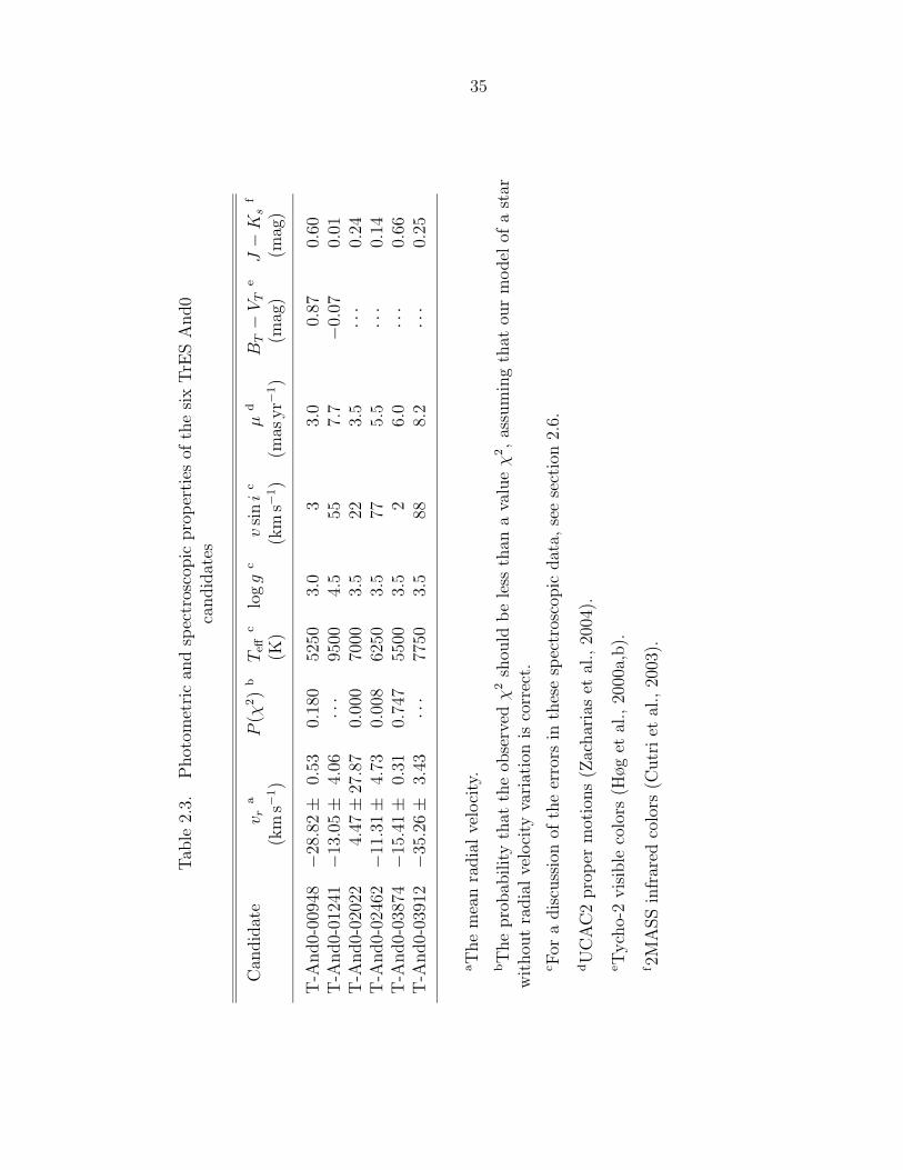
35

Tab

le2.

3.P

hot

omet

ric

and

spec

tros

copic

pro

per

ties

ofth

esi

xTrE

SA

nd0

candid

ates

Can

did

ate

v ra

P(χ

2)

bT

eff

clo

gg

cv

sin

ic

µd

BT−

VT

eJ−

Ks

f

(km

s−1)

(K)

(km

s−1)

(mas

yr−

1)

(mag

)(m

ag)

T-A

nd0-

0094

8−

28.8

2±

0.53

0.18

052

503.

03

3.0

0.87

0.60

T-A

nd0-

0124

1−

13.0

5±

4.06

···

9500

4.5

557.

7−

0.07

0.01

T-A

nd0-

0202

24.

47±

27.8

70.

000

7000

3.5

223.

5···

0.24

T-A

nd0-

0246

2−

11.3

1±

4.73

0.00

862

503.

577

5.5

···

0.14

T-A

nd0-

0387

4−

15.4

1±

0.31

0.74

755

003.

52

6.0

···

0.66

T-A

nd0-

0391

2−

35.2

6±

3.43

···

7750

3.5

888.

2···

0.25

aT

he

mea

nra

dia

lve

loci

ty.

bT

he

pro

bab

ility

that

the

obse

rved

χ2

shou

ldbe

less

than

ava

lue

χ2,as

sum

ing

that

our

model

ofa

star

wit

hou

tra

dia

lve

loci

tyva

riat

ion

isco

rrec

t.

cFor

adis

cuss

ion

ofth

eer

rors

inth

ese

spec

tros

copic

dat

a,se

ese

ctio

n2.

6.

dU

CA

C2

pro

per

mot

ions

(Zac

har

ias

etal

.,20

04).

eT

ych

o-2

vis

ible

colo

rs(H

øget

al.,

2000

a,b).

f2M

ASS

infr

ared

colo

rs(C

utr

iet

al.,

2003

).

36

Table 2.4. Details of spectroscopic observations of the six TrES And0 candidates

Candidate Time of Observation Photometric Orbital Phase Radial VelocityHJD km s−1

T-And0-009482453276.8749 0.46 −28.16 ± 0.362453277.8530 0.33 −29.19 ± 0.402453278.8236 0.20 −29.00 ± 0.32

T-And0-01241 2453276.8062 0.73 −13.05 ± 4.06

T-And0-02022

2453276.8642 0.80 35.46 ± 0.742453301.8475 0.07 −14.14 ± 0.992453334.7734 0.02 − 3.77 ± 0.942453548.9711 0.21 −39.63 ± 1.122453575.9740 0.90 24.54 ± 1.052453576.9683 0.11 −20.34 ± 1.162453626.9029 0.65 23.98 ± 1.132453627.9043 0.86 29.37 ± 0.702453628.8392 0.06 − 9.31 ± 0.812453629.8518 0.27 −42.28 ± 1.122453630.8361 0.48 −15.29 ± 1.242453631.8335 0.69 30.93 ± 0.862453632.8135 0.90 24.80 ± 0.872453633.8047 0.10 −20.66 ± 1.022453636.8830 0.75 37.44 ± 0.862453779.5864 0.84 29.64 ± 1.14

candidate (see Table 2.3) from the template parameters that gave the highest average

peak correlation value over all the observed spectra.

37

Table 2.4 (cont’d)

Candidate Time of Observation Photometric Orbital Phase Radial VelocityHJD km s−1

T-And0-024622453276.8864 0.11 − 7.55 ± 1.402453686.7688 0.18 −14.50 ± 3.74

T-And0-03874

2453276.8192 0.17 −15.81 ± 0.442453277.8381 0.55 −15.15 ± 0.412453301.8342 0.59 −15.09 ± 0.432453334.7619 0.00 −15.50 ± 0.43

T-And0-03912 2453276.8398 0.22 −35.26 ± 3.43

For the three candidates with low stellar rotation, v sin i < 50 km s−1, we ob-

tained several spectra over different observing seasons to determine the radial veloc-

ity variation of each star. Table 2.4 details our spectroscopic observations. For these

slowly rotating candidates, the typical precision for our spectroscopic parameters is

∆Teff = 150 K, ∆ log g = 0.5, ∆v sin i = 2 km s−1, and ∆V = 0.5 km s−1. The preci-

sion of the estimates degrades for stars with large v sin i values or few spectroscopic

observations.

We obtained high-precision photometry of T-And0-03874 on UT 2004 Decem-

ber 19 using the Minicam CCD imager at the FLWO 1.2-meter telescope on Mount

Hopkins, Arizona. Minicam consists of two 2248 × 4640 pixels thinned, backside-

illuminated Marconi CCDs mounted side-by-side to span a field of approximately

20.4′ × 23.1′ bisected by a narrow gap. We employed 2 × 2 pixels binning for an

effective plate scale of 0.6′′ pixel−1 and read out each half CCD through a separate

amplifier. We offset the telescope to place T-And0-03874 centrally on one amplifier

region and autoguided on the field. We obtained concurrent light curves in three fil-

ters by cycling continuously through the SDSS g, r, and z filters with exposure times

of 90, 45, and 90 s respectively. The seeing was poor (FWHM ∼ 3′′–7′′) and varied

throughout our observations. Unfortunately, high winds forced us to close the dome

during the night and we obtained only partial coverage of the predicted event. Late

38

in the scheduled observations, we re-opened for a short time.

We subtracted the overscan bias level from each image and divided each by a

normalized flat field constructed from the filtered mean of twilight sky exposures. To

construct a light curve of T-And0-03874 and neighboring bright stars, we located the

stars in each image. We measured stellar fluxes in a circular aperture and subtracted

the sky as estimated by the median flux in an annulus centered on the star (iteratively

rejecting deviant sky pixel values). We used a relatively large 12′′ radius aperture

and sky annulus with inner and outer radii of 15′′ and 27′′ respectively in an effort to

reduce systematic errors arising due to the poor and variable seeing conditions. We

first corrected the flux of each star by an amount proportional to its air mass in each

exposure by using extinction coefficients for each filter based on previous experience

with Minicam photometry. Second, we selected a group of bright, uncrowded stars

near T-And0-03874 as potential comparison stars. In each exposure we calculated

the mean flux of the comparison stars weighted according to brightness. We assumed

that any variations in this mean flux represented extinction in each image and used

them to apply corrections to each light curve. We then inspected by eye the light

curve of each comparison star and fit the light curves to models of constant brightness

to find χ2 statistics. We removed from our group of comparison stars any star that

showed significant variations. We recalculated the extinction corrections iteratively

in this manner until we achieved no variation in the comparison star light curves.

We accepted 29, 32, and 4 comparison stars for the g-, r-, and z-band light curves

respectively. Finally, we normalized the flux in the light curves of T-And0-03874 with

respect to the out-of-eclipse data.

2.6 Rejecting False-Positive Detections

Based on our detailed investigations of the candidates, we eliminated each And0

candidate as follows.

In the case of T-And0-00948, the TrES light curve (figure 2.3) shows a secondary

eclipse. The low surface gravity (log g = 3.0) is that of a distant giant star, consistent

39

with the red color J−Ks = 0.60 mag (since the majority of stars with J−Ks > 0.5 mag

are expected to be giants, see, e.g., Brown, 2003). There was no observed variation

in the radial velocity of this candidate (vr = −28.82 km s−1). T-And0-00948 is most

likely the primary star of a diluted triple system.

Upon further examination of the individual light curves for T-And0-01241, we

noticed that only Sleuth had observed transit events for this system. Neither PSST

nor STARE had observed this field during the time of the Sleuth transit events,

preventing a comparison of the light curves. Based on the Sleuth data, we predicted

the times of transits during the entire TrES And0 campaign. STARE did observe

T-And0-01241 at a time at which it was predicted to transit but did not observe the

transit. It was therefore possible that this was a photometric false positive. However,

we did not pursue this further, as we obtained sufficient evidence from the follow-up

spectroscopy to discount the system. A dwarf with log g = 4.5, the star has the high

effective temperature (Teff = 9500 K) and blue colors (J −Ks = 0.01 mag) of an early

A star. Figure 2.4b shows the nearly featureless spectrum of this star. For such a

large star with a radius R ∼ 2.7 R⊙, the observed transit depth of 0.9% indicates a

non-planetary size (R = 2.5 RJup) for the eclipsing body.

The radial velocity of T-And0-02022 varies with an amplitude corresponding to a

stellar-mass companion. We determined this system to be an eclipsing binary, com-

prising a slightly evolved F dwarf and an M dwarf. This system has a mass function

f(M) = 0.0304±0.0013 M⊙ and an eccentricity of 0.027±0.014. Assuming an orbital

inclination of i ∼ 90◦ and a mass of 1.6 M⊙ consistent with the effective temperature

(Teff = 7000 K), we estimated the mass of the companion to be m = 0.5 M⊙. Fig-

ure 2.5 shows the radial velocity orbit. The circular orbit of T-And0-02022 allows us

to constrain the stellar radius, independent of our derived spectral type and luminos-

ity class. The circular orbit implies orbital synchronization and orbital-rotation axes

alignment, since circularization has the longest timescale of these processes. (This

should apply except for very low mass secondaries; see Hut, 1981 for a derivation

of these timescales for close binary systems and a comparison for different binary

mass ratios and moments of inertia of the primary star.) We can therefore assume

40

(a) (b)

(c) (d)

(e) (f)

Figure 2.4 Sample spectra of the And0 TrES candidates obtained with the CfADigital Speedometers on the FLWO 1.5-meter telescope: (a) T-And0-00948 has thelow surface gravity of a giant star, (b) T-And0-01241 has the featureless spectrum ofan A-type star, (c) T-And0-02022 is an evolved F dwarf, (d) T-And0-02462 and (e)T-And0-03912 display broadened lines due to the rapid rotation of these stars, and(f) T-And0-03874 is an early K-type dwarf.

41

ORBITAL PHASE0 .2 .4 .6 .8 1

-40

-20

0

20

40

Figure 2.5 Radial velocity orbit of T-And0-02022 as determined from our DigitalSpeedometer spectra. This system was quickly rejected as a candidate transitingplanet after the large radial velocity variation was determined from initial spectro-scopic observations. Additional epochs produced a precise orbit with an eccentricityof e ∼ 0.03. An initial mass estimate of 0.5 M⊙ was derived for the companion.Future photometry will lead to more precise mass determination for both componentstars (see text for a discussion).

42

that the stellar rotation period is the same as the orbital period of 4.7399 days. We

then use the observed rotational broadening (v sin i = 22 km s−1) to estimate the

radius of the star to be 2.0 R⊙. Future photometric observations of this systems

with KeplerCam (Szentgyorgyi et al., 2005) are planned to more precisely measure

the eclipse depth and to derive the radius and true mass of each star in this binary

(J. M. Fernandez et al. 2007, in preparation).

T-And0-02462 is a rapid rotator with v sin i = 77 km s−1 and displays rotationally

broadened lines (see figure 2.4d), limiting the possibility of detecting the radial ve-

locity variation caused by a planet. Regardless, we inferred a binary nature for this

candidate using the combined TrES data, which proved essential in identifying this

false positive. Our initial Sleuth light curve of T-And0-02462 showed no evidence of a

stellar-mass companion, and we derived a BLS best-fit period of 1.5347 days. On ex-

amining the TrES light curve of T-And0-02462 (see figure 2.3), we noticed a secondary

eclipse. Also, the BLS best-fit period for our TrES observations of T-And0-02462 is

twice that derived from the Sleuth data alone. When we reexamined the Sleuth data

phased to the TrES period, the secondary eclipse is not visible due to inadequate

coverage at that phase. This resulted in a derived period for the Sleuth data half

that of the true period.

The red color of T-And0-03874 (J−Ks = 0.66 mag) and the effective temperature

(Teff = 5500 K) calculated from the spectrum shown in figure 2.4e are consistent with

an early K-type star. The radial velocity of T-And0-03874 was observed to remain

constant at −15.53 km s−1. However, the low estimated surface gravity (log g = 3.5)

suggested this star is a giant star and part of a diluted triple. The photometric

follow-up (see figure 2.6) failed to recover transits of T-And0-03874, but did observe

a nearby eclipsing binary T-And0-02943 undergoing a deep eclipse at the predicted

transit time (also shown in figure 2.6). When we examined our TrES observations

for T-And0-02943, we saw that the period of this eclipsing binary was that originally

derived for T-And0-03874, namely 2.654 days. This eclipsing system lies 45′′ away

from T-And0-03874, comparable to the PSF radius of our TrES aperture photometry

(30′′; 3 pixels). The angular resolution (∼1′′ pixel−1) of the 1.2-meter photometry is

43

Figure 2.6 Follow-up g-, r-, and z-band photometry with the FLWO 1.2-meter tele-scope of T-And0-03874 (squares) and a neighboring star (diamonds), designatedT-And0-02943, that lies 45′′ away. (The inset 2′ × 2′ Digitized Sky Survey imageshows T-And0-03874 at the center and T-And0-02943 above, to the north.) The fluxfrom each star has been normalized using the out-of-eclipse data, and an offset ap-plied for the purpose of plotting. Inclement weather prevented complete coverage ofthe predicted eclipse event. Nevertheless, it is evident that T-And0-02943 displays adeep (>14%) eclipse, whereas the flux from T-And0-03874 is constant. The observedapparent transits of T-And0-03874 were the result of the blending of the light fromthese two systems. With a FWHM for T-And0-02943 of ∼2.5 pixels (∼25′′), some ofthe light from this star was within the photometric aperture radius (3 pixels; ∼30′′)of T-And0-03874.

44

Figure 2.7 TrES photometry of T-And0-03874 and the neighboring eclipsing binaryT-And0-02943, phased to the best-fit period (2.6540 days) for T-And0-03874 derivedby the box-fitting algorithm. Both stars show eclipses with the same orbital periodand epoch. The ∼1% transit-like event detected in the light curve of T-And0-03874was the result of the blending of light from this star and from T-And0-02943, whichlies 45′′ away, comparable to the 30′′ radius of the TrES PSF.

45

higher than that of the original TrES photometry (9.9′′ pixel−1); hence the light from

these two systems is blended in our TrES observations (see figure 2.7) but is resolved

in the 1.2-meter photometry.

Finally, the observed parameters for T-And0-03912 (log g = 3.5, Teff = 7750 K,

J − Ks = 0.25 mag) again imply a large stellar radius (R ∼ 1.8 R⊙). In order to

produce the 0.9% transit, a companion radius of 1.5 RJup is required. This is consistent

with the large radii of the transiting planets HAT-P-1b (Bakos et al., 2007), and

WASP-1b (Charbonneau et al., 2007b), although we have not ruled out the possibility

of a blend. Regardless, the star T-And0-03912 is rapidly rotating (v sin i = 88 km s−1;

see figure 2.4f), making precise radial-velocity follow-up extremely difficult.

2.7 Maximizing the Yield from TrES

The Trans-atlantic Exoplanet Survey monitors ∼30,000 stars each year from which

we identify ∼30 stars whose light curves show periodic eclipses consistent with the

passage of a Jupiter-sized planet in front of a Sun-like star. In order to eliminate

astrophysical false positives, we have established a procedure of multi-epoch pho-

tometric and moderate-precision spectroscopic follow-up. Surviving candidates are

optimal targets for high-precision multi-epoch radial velocity measurements that will

yield the masses of planetary companions.

The TrES field in Andromeda was one of the first of our fields for which we

combined the data from the three TrES telescopes. We have demonstrated here the

benefit of this: the improved transit visibility, the increase in number of stars with low

rms residual, and the confirmation of transit events observed by different telescopes.

It has also provided us with several examples of the astrophysical false positives that

will be encountered in any ground-based, wide-field transit survey, all of which were

rejected as a result of follow-up observations. Based on our experience with these

false positives, we refined the criteria by which we identify TrES planet candidates.

For each new transit candidate, we now search our data set for a nearby eclipsing

binary with a similar period as derived by the BLS algorithm in order to check for

46

blends. We also examine the transit light curve phased using integer multiples or

fractions of the BLS orbital period.

In comparison to other, more subtle examples (such as those discussed by

O’Donovan et al. 2006b [see chapter 3], Torres et al. 2004b, and Mandushev et al.

2005), these transit candidates were easily identified as false positives. These exam-

ples demonstrate the need for both spectroscopic and photometric follow-up of transit

candidates, which may be accomplished with the one-meter class telescopes, on which

time is readily available. This ensures that the precious resource of ten-meter spec-

troscopy is used efficiently.

47

Chapter 3

Rejecting Astrophysical FalsePositives from the TrES TransitingPlanet Survey: The Example ofGSC 03885-008291

Abstract

Ground-based wide-field surveys for nearby transiting gas giants are yielding far fewer

true planets than astrophysical false positives, some of which are difficult to reject.

Recent experience has highlighted the need for careful analysis to eliminate astronom-

ical systems in which light from a faint eclipsing binary is blended with that from a

bright star. During the course of the Trans-atlantic Exoplanet Survey, we identified

a system presenting a transit-like periodic signal. We obtained the proper motion

and infrared color of this target (GSC 03885-00829) from publicly available catalogs,

which suggested this star is an F dwarf, supporting our transit hypothesis. This

spectral classification was confirmed using spectroscopic observations from which we

determined the stellar radial velocity. The star did not exhibit any signs of a stel-

lar mass companion. However, subsequent multicolor photometry displayed a color-

dependent transit depth, indicating that a blend was the likely source of the eclipse.

We successfully modeled our initial photometric observations of GSC 03885-00829 as

the light from a K-dwarf binary system superimposed on the light from a late F-dwarf

1This chapter has been published previously as O’Donovan et al. 2006b, ApJ, 644, 1237.

48

star. High-dispersion spectroscopy confirmed the presence of light from a cool stellar

photosphere in the spectrum of this system. With this candidate, we demonstrate

both the difficulty in identifying certain types of false positives in a list of candidate

transiting planets and our procedure for rejecting these imposters, which may be

useful to other groups performing wide-field transit surveys.

3.1 Transits versus Blended Eclipses

The discovery of the 169 known extrasolar planets2 has greatly enhanced our under-

standing of planetary systems. Most of these extrasolar planets have been identified

from Doppler surveys that search for the radial velocity variation of a star caused by

the presence of a gas giant. These observations can estimate the period and eccen-

tricity of the planetary orbit, and provide a lower limit for the planetary mass relative

to that of the star. Assuming that the stellar mass can be precisely determined, per-

haps by comparing the stellar spectra to stellar atmosphere models (such as Kurucz,

1993), the minimum mass of the planet can be derived. The diversity of these plane-

tary systems has drastically altered our theoretical appreciation of their morphology

and evolution, including the existence of “hot Jupiters”, Jupiter-sized planets with

periods of a few days that experience high insolation from the nearby star. However,

less is known about the nature of the planets themselves, except for the cases when

a hot Jupiter was observed to pass in front of a dwarf star. By observing such a

transit (as was first suggested by Struve 1952), we can estimate the radius of the

transiting planet from the fraction of starlight the planet blocks during the transit

and the radius of the star itself, which must be measured from stellar model fits to

spectra of the star. For a transit to occur, the planetary orbital inclination must be

approximately 90◦; this implies that the Doppler limit for the planetary mass must

be close to the actual mass of the planet. At the time of writing, we have estimates

for the radii and masses of 9 planets from transit observations similar to those first

2Updates available from the Extrasolar Planets Encyclopaedia:http://www.obspm.fr/planets/ .

49

successfully performed by Charbonneau et al. (2000) and Henry et al. (2000). These

estimates provide constraints for the competing theories of planetary formation. For

example, the recently discovered transiting “hot Saturn” HD 149026 b has a mass and

radius that imply the planet has a large core (approximately 70 M⊕; Sato et al. 2005;

Charbonneau et al. 2006). It is hypothesized that this planet must have formed via

core accretion (Pollack, 1984; Pollack et al., 1996), rather than through gravitational

instability (Boss, 1997). However, not every observation of a transiting planet can be

explained by current models of close-in giant planets experiencing high stellar insola-

tion. The transiting planet HD 209458b has a radius larger than other planets of its

mass and larger than the predicted radii (see Laughlin et al., 2005, and references

therein; Deming et al. 2005b).

Several wide-field photometric surveys with the goal of identifying nearby tran-

siting planets are currently active. Our Trans-atlantic Exoplanet Survey3 (TrES) is

a network of three ten-centimeter telescopes: Sleuth (located at Palomar Observa-

tory, California; O’Donovan et al. 2004), the Planet Search Survey Telescope (PSST,

Lowell Observatory, Arizona; Dunham et al. 2004), and the STellar Astrophysics and

Research on Exoplanets4 telescope (STARE, Tenerife, Spain; Alonso et al. 2004b).

The TrES campaign, together with other wide-field surveys such as the HAT network

(Bakos et al., 2002) and SuperWASP (Street et al., 2003), are monitoring thousands

of nearby bright stars (9 ≤ V ≤ 13). We hope to find recurring eclipses with the short

period and small amplitude corresponding to a transiting hot Jupiter. The bright-

ness of the target stars facilitates both the photometric precision and the follow-up of

any identified transiting planets using space-borne telescopes. Examples of detailed

follow-up observations include the measurement of several chemical abundances in the

atmosphere of HD 209458b (Charbonneau et al., 2002; Vidal-Madjar et al., 2003) and

the first direct detections of emitted planetary radiation (Charbonneau et al., 2005;

Deming et al., 2005b).

Many astrophysical systems exist that mimic the light curve of a transiting hot

3See http://www.astro.caltech.edu/~ftod/tres/ .4See http://www.hao.ucar.edu/public/research/stare/stare.html .

50

Jupiter. Due to the mass-radius degeneracy for bodies with masses between 0.001 and

0.1M⊙, the depth of an eclipse of a solar-type star by a hot Jupiter, a brown dwarf

or an M dwarf star will be about 1% in each case, despite the large range in mass.

Grazing incidence eclipsing binaries may also exhibit comparable eclipse depths. For

wide-field ground-based surveys, the frequency of the false positives is greater than

the frequency of detection of true transiting planets, by at least an order of magnitude.

As part of TrES, we typically identify 10–20 of these transit-like photometric signals

out of 15,000–25,000 stars (10 < V < 15) in each 6◦×6◦ target field of view (b ∼ 15◦;

see, e.g., Dunham et al., 2004), and similar yields should be expected from other wide-

field ground-based surveys. This number (which is dependent on the density of star

counts, and hence the Galactic latitude) is consistent with theoretical predictions.

For example, Brown (2003) predicts that for every 25,000 stars observed, we will find

10 false positives and only one true transiting planet. This assumes that we must

observe three transit events for each candidate and is dependent on the visibility

of transits throughout the observation run. The low yield of planets necessitates

a rigorous routine of follow-up observations and detailed analysis to eliminate all

possible alternatives to the planet hypothesis. One straightforward method to reduce

the number of false positives is to obtain multi-epoch spectroscopy of each candidate

and measure radial velocities with a precision of ∼1 km s−1. From this we can identify

targets with companions of stellar, rather than planetary, mass (see, e.g., Latham,

2003; Charbonneau et al., 2004). We can also estimate the luminosity class of the

target star to single out and reject giants.

The blending of the light from an edge-on binary system with that from a third

star can also be mistaken for a transit. Brown (2003) predicts that half of the false

positives from a typical wide-field survey will be of this type; the other half will

be grazing eclipsing binaries. Blends can be much more difficult to identify. The

faintness of the binary compared to the third star can prevent the detection of the

radial velocity variations of the binary. These variations are also masked by the

rotationally broadened spectral lines of the rotationally synchronized binary stars.

However, if the binary has a significant difference in effective temperature from that of

51

the third star, the eclipse depths should display a strong color dependence, unlike the

color-independent transits of a (dark) planet across a single star. Nevertheless, there

has been recent experience of blends with color-independent eclipse depths. In the

case of OGLE-TR-33 (Torres et al., 2004b) and GSC 01944-02289 (Mandushev et al.,

2005), both candidates (a suspected planet and brown dwarf, respectively) showed

color-independent eclipse depths, and yet were subsequently discovered to be blended

systems. Evidence for the presence of an eclipsing binary was found from a careful

analysis of the spectral line shapes, prompting the authors to compare the photometric

data to simulations of blends. OGLE-TR-33 was shown to be a hierarchical triple

consisting of a bright F6 dwarf and an F4+(K7–M0) binary. The blend model for

GSC 01944-02289 comprises an F5 primary and a G0+M3 binary. In both cases, the

similarity in color between the primary star and the brightest member of the binary

explains the constant eclipse depth at different wavelengths. The high occurrence

of such false positives and the difficulty in rejecting them requires a detailed study

of candidates before any announcement is made, as was done in the case of TrES-1

(Alonso et al., 2004a) and OGLE-TR-56b (Torres et al., 2004a).

Here we discuss a promising candidate, GSC 03885-00829, from one of our target

fields. Initial photometric (section 3.2) and spectroscopic (section 3.3) monitoring of

this candidate strongly suggested that we were observing a Saturn-sized companion

transiting a solar type star every 1.441 days with a transit depth of approximately

6 mmag. However, follow-up photometry (section 3.4) displayed a slight color depen-

dence as might be caused by a blend, and we were able to model our photometry

using simulations of blended eclipsing binaries (section refcha:gsc:sec:blend). Our

best-fit model consists of a bright F dwarf and a K-dwarf binary, and we were able

to identify the presence of light from the binary in the spectrum of GSC 03885-00829

(section 3.6). The faintness of the binary system prevents us from identifying the

presence of asymmetric spectral lines, as was done by Torres et al. (2004b) and

Mandushev et al. (2005). In this case, only multicolor observations provided us with

the necessary evidence to call into question the planetary nature of this candidate.

52

3.2 TrES Telescope Observations of

GSC 03885-00829

In 2004 March, we commenced observations of a 6◦×6◦ target field in Draco. The field

is centered on our V = 4.8 guide star HD 151613 (α = 16h45m17.82s, δ = +56◦46′54.7′′

J2000.0). Between UT 2004 March 29 and June 22, we observed this field nightly with

Sleuth at Palomar Observatory (California) and with PSST at Lowell Observatory

(Arizona). STARE, in Tenerife (Spain), did not observe this field as it was undergo-

ing repairs at this time. A total of 15,854 photometric exposures of 90 s each were

obtained through either a Sloan r filter (Sleuth) or a Kron-Cousins R filter (PSST).

We bias-subtracted and flat-fielded the images of our target field once the data

were transferred from the observatory computers. We performed the calibration of

the Sleuth data using customized IDL routines; we calibrated the PSST data using

the zerocombine, ccdproc, and flatcombine tasks in the IRAF5 package (Tody,

1993). We reduced the Sleuth and PSST photometric data separately as follows

using our difference image analysis (DIA) pipeline (described in Dunham et al., 2004,

and based in part on Alard, 2000).

We created our reference image for the field from images obtained at low air

mass on a photometric night during dark time. We obtained a standard list of

stars from this image using profile-fitting (point-spread function, PSF) photometry

(DAOPHOT II/ALLSTAR; Stetson 1987, 1992). We calculated the equatorial coor-

dinates (α, δ) of these stars by matching a subset with the stars listed in the Tycho-2

Catalog (Høg et al., 2000b) and then spatially interpolated all of the science images

so that the star coordinates from each image matched those from our standard star

list.

We produced the master image for the Sleuth data set by combining 19 of our

best-quality interpolated images; we combined 17 images to create the corresponding

PSST master image. We subtracted each interpolated image from this master image.

5IRAF is distributed by the National Optical Astronomy Observatories, which are operated bythe Association of Universities for Research in Astronomy Inc. under cooperative agreement withthe National Science Foundation.

53

We used aperture photometry on the resultant difference images (using the centroids

derived for the standard star list) to estimate the flux of each star in each image. We

produced time series consisting of the differences between the magnitude of a star in

the reference image and the magnitude of that star in each target image in turn. We

decorrelated these light curves as follows to remove systematic effects typical of wide-

field surveys, such as those caused by changing atmospheric conditions throughout

the night. We listed the stars in order of brightness, and divided the list into batches

of 500. We computed the least-squares fit to the light curve of a given star from a

linear combination of the other light curves in that batch. We then subtracted this

least-squares fit from the light curve of the star.

In our previous studies (Alonso et al., 2004a; Mandushev et al., 2005;

Creevey et al., 2005), we presented separate light curves from one of the TrES tele-

scopes. For this field, we combined the two data sets. For a given star on the Sleuth

standard star list, we calculated the angular distances between that star and the PSST

standard stars. We matched the Sleuth star with a PSST star if the angular distance

was less than 5′′ (0.5 pixels). Due to the difference in the selected filter and the

telescope pointing between the two sites, some stars were unique to a given standard

star list, and no match was found. We appended the time series for each matched

PSST star to the corresponding Sleuth time series, and reordered the combined time

series chronologically. The data for the unmatched PSST stars were simply added to

the resulting data set.

In order to reduce the computational intensity of our transit search, we averaged

the combined time series in 9-minute-wide bins to obtain 2996 binned observations.

Since central transits should last 3 hr (see section 1.2.2), this did not significantly

sacrifice temporal resolution of potential transit events. For ∼10,000 stars, the rms

scatter of the binned data was below 0.04 mag. We performed a search of the time

series of these stars using the box-fitting least-squares (BLS) transit-search algorithm

(Kovacs, Zucker, & Mazeh 2002, see appendix C) to identify periodic transit events.

The BLS algorithm calculates a Signal Detection Efficiency (SDE; see Kovacs et al.,

2002) for each candidate, which denotes how significant the detection is. We identified

54

Figure 3.1 Binned TrES r-band light curve of GSC 03885-00829, folded with the pho-tometric period of 1.441 days computed using the box-fitting least-squares algorithm.Overlaid is the corresponding box transit model.

candidates based on this SDE, followed by a visual inspection.

Many of the candidates identified for this field show V-shaped eclipse, a possi-

ble ellipsoidal variability, or have large depths, making it likely that they are not

transiting planets, but rather eclipsing binaries. However, we promptly identified a

promising candidate. When the data for this star were folded with the photometric

orbital period of 1.441 days (calculated using the BLS algorithm), the resultant light

curve (figure 3.1) displayed a shallow and flat-bottomed transit, and no noticeable

ellipsoidal variability out of transit. The depth (∼6 mmag) and duration (1.4 hr) of

the occultation are consistent with a Saturn-sized planet transiting a solar-type star.

The SDE for this candidate (∼20) was high relative to that calculated for typical

TrES candidates (∼10–15).

Supporting data from online catalogs provided further evidence of the planetary

nature of this eclipse. Using the SIMBAD6 database, we identified our candidate

as the star GSC 03885-00829 (see Table 3.1). The infrared colors (2MASS J − Ks,

J − H; Cutri et al. 2003) and optical (B − V ) colors of this star are near-solar,

roughly consistent with the stellar parameters inferred from our transit observations.

This star displays significant proper motion (26 mas yr−1 from the USNO-B Catalog;

Monet et al. 2003), suggesting it is a nearby dwarf. As a first check of the possibility

of contamination of light from a nearby star, we verified that there is no bright star

6See http://simbad.harvard.edu/ .

55

Table 3.1. Data for GSC 03885-00829

Parameter Value

R.A. (J2000.0) 16h52m33.7s

Decl. (J2000.0) +57◦58′27′′

GSC 03885-008292MASS 16523368+5758262

V a (mag) 10.465 ± 0.001B − V a (mag) 0.612 ± 0.001V − RC

a (mag) 0.371 ± 0.003V − IC

a (mag) 0.743 ± 0.001J b (mag) 9.197 ± 0.018J − H b (mag) 0.337 ± 0.023J − Ks

b (mag) 0.440 ± 0.026

Period c (days) 2.88244 ± 0.00046T2

d (HJD) 2453529.833 ± 0.009Depth (r mag) 0.006 ± 0.003

aSee section 3.4 for a discussion of errors.

bFrom the 2MASS Catalog (Cutri et al., 2003).

cThe period of the suspected candidate planetwas 1.d44122 ± 0.d00023.

dThe time of the secondary eclipse of the binary,and the central transit time of the candidate.

56

visible on the Digitized Sky Survey7 (DSS) images within our aperture radius (≤ 30′′).

With due enthusiasm, we proceeded to obtain follow-up observations of this excit-

ing candidate, with the goal of rejecting the possibility that this was not a transiting

planet.

3.3 Spectroscopic Follow-up of GSC 03885-00829

We confirmed that GSC 03885-00829 was an isolated dwarf star by spectroscopically

monitoring this candidate. We observed GSC 03885-00829, together with other can-

didates from this TrES field, with the Harvard–Smithsonian Center for Astrophysics

(CfA) Digital Speedometer (Latham, 1992), operated on the 1.5 m Tillinghast reflec-

tor at the F. L. Whipple Observatory (FLWO) on Mount Hopkins, Arizona. The

spectral coverage was 45 A centered on 5187 A at a resolving power of λ/∆λ ≈ 35,000

(a resolution of 8.5 km s−1). We observed this particular target on UT 2005 May 18,

May 20, and May 21, at an orbital phase 0.52, 0.86, and 0.50, respectively (calculated

using the orbital ephemeris of the planet; see Table 3.1, footnote c).

Radial velocities were obtained by cross-correlation using templates chosen from

a library of synthetic spectra computed for us by J. Morse and based on the model

atmospheres of R. L. Kurucz (J. Morse & R. L. Kurucz, 2004, private communi-

cation; see figure 3.3). The typical precision of a single velocity measurement is

0.5 km s−1. We measured the radial velocity to be constant (−38.48 km s−1 with an

rms of 0.28 km s−1) within our errors. These measurements indicate that the tar-

get star is not gravitationally bound to a massive stellar companion. Various stellar

parameters were estimated, again by cross-correlating these spectra against a grid

of templates from our spectral library, seeking the best match. Assuming a solar

metallicity, we estimated the effective temperature to be Teff = 6150 K and the sur-

face gravity to be log g ≈ 4.4, that suggested this was a late F-dwarf star, consistent

7The Digitized Sky Survey (http://archive.stsci.edu/dss/) was produced at the Space Tele-scope Science Institute under US Government grant NAG W-2166. The images of these surveys arebased on photographic data obtained using the Oschin Schmidt Telescope on Palomar Mountainand the UK Schmidt Telescope. The plates were processed into the present compressed digital formwith the permission of these institutions.

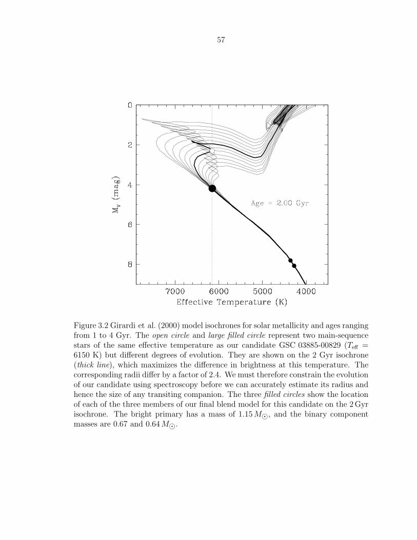
57

Figure 3.2 Girardi et al. (2000) model isochrones for solar metallicity and ages rangingfrom 1 to 4 Gyr. The open circle and large filled circle represent two main-sequencestars of the same effective temperature as our candidate GSC 03885-00829 (Teff =6150 K) but different degrees of evolution. They are shown on the 2 Gyr isochrone(thick line), which maximizes the difference in brightness at this temperature. Thecorresponding radii differ by a factor of 2.4. We must therefore constrain the evolutionof our candidate using spectroscopy before we can accurately estimate its radius andhence the size of any transiting companion. The three filled circles show the locationof each of the three members of our final blend model for this candidate on the 2 Gyrisochrone. The bright primary has a mass of 1.15M⊙, and the binary componentmasses are 0.67 and 0.64M⊙.

58

Figure 3.3 Sample spectrum of GSC 03885-00829 (which includes the Mg I b triplet)and the corresponding cross-correlation function.

59

with the proper motion and photometric colors, and with our transit hypothesis. The

formal stellar rotation we derived (v sin i ≈ 1 km s−1) is actually below our spectral

resolution. The surface gravity suggests that the star is unevolved. This constraint

is important, as this star lies within the range of effective temperatures for which an

ambiguity exists as to the corresponding mass of the star while on the main sequence,

depending on the degree of evolution. An illustration of this ambiguity is shown in

figure 3.2, where the two locations denoted by the open circle and large filled circle

have the same effective temperature as GSC 03885-00829 but rather different lumi-

nosities. The particular age of the isochrone for this figure was selected to show

this difference more clearly. The fainter (lower) location corresponds to an unevolved

main-sequence star (log g = 4.34) of mass 1.15M⊙, whereas the brighter location is

for a star near the end of the hydrogen-burning phase and has a surface gravity of

log g = 3.68 and a mass of 1.61M⊙. The radii differ by a factor of about 2.4. From

this example, we see that, without a surface gravity constraint, we cannot be sure of

the radius of our target star, preventing our discriminating between a planetary and

a stellar transiting companion.

3.4 Photometric Follow-up of GSC 03885-00829

Although we had found no evidence of a stellar mass companion from our radial

velocity measurements, the possibility remained that the observed transits were in fact

the eclipses of a faint binary whose light was blended with that from the bright F dwarf

due to the large pixel sizes of our detectors. Follow-up observations of higher angular

resolution might resolve such a blended system. A possible wavelength dependence

of the eclipse depth from multicolor observations would also provide evidence of a

blend. We organized a follow-up photometric campaign to observe multiple transits

of GSC 03885-00829 using D > 20′′ (0.50 m) telescopes and several different filters.

High precision photometry of GSC 03885-00829 was made on UT 2005 June 8

using the 1.2 m FLWO telescope (Arizona). For this clear, photometric night, we used

MiniCam, a two CCD mosaic, each array being 2048×4608 pixels. Observations were

60

Figure 3.4 Our follow-up photometry of GSC 03885-00829 near the predicted time oftransit. The observations were folded using the orbital ephemeris of the planet (seeTable 3.1, footnote c). Each plot is labelled with the corresponding telescope (seetext) and the filter bandpass. The predicted transit events were observed, but anincrease in eclipse depth with increasing wavelength is apparent.

61

binned 2× 2 for a faster duty cycle. A Sloan g filter was used, with an exposure time

of 30 s and a corresponding duty cycle of ∼50.5 s. The telescope was de-focused to a

FWHM of ∼15 pixels (∼9′′) to allow greater photon counts per given exposure without

saturation. Spreading the star image also serves to reduce pixel-to-pixel variations

that may not be completely removed by flat-fielding. A total of 561 photometric

measurements of the field were made over a total of 7.875 hr. The differential light

curve of our target star was obtained using aperture photometry of this star and one

of the observed reference stars. We corrected for the effect of differential extinction on

the time series by fitting the out-of-eclipse data. The resultant light curve was then

converted to flux units (see figure 3.4). These follow-up photometric observations were

made over a year after our TrES images. We used this separation in time to obtain

a more accurate photometric ephemeris for our candidate, Tc(HJD) = 2453529.833 +

1.44122 × E (see Table 3.1).

GSC 03885-00829 was observed on the night of UT 2005 June 13 at the 0.82-meter

IAC-80 telescope at the Observatorio del Teide (Tenerife, Spain), using its 1024×1024

pixels CCD and a Johnson R filter. To achieve better photometric precision, a slight

defocus was applied, in order to image stars with a FWHM of ∼4′′. Exposures times

of 22 s were used, and the readout time using a 2 × 2 pixels binning was ∼10 s. The

images were bias and flat-field corrected, and aperture photometry was applied using

the package for optimal aperture photometry vaphot (Deeg & Doyle, 2001). Nine

reference stars were used to build an ensemble reference star. The dispersion of the

data points is larger at the end of the night as the star was closer to the horizon.

We corrected for differential extinction; figure 3.4 shows the derived differential light

curve.

We obtained BV (RI)C observations of GSC 03885-00829 on UT 2005 June 5

with the Lowell Observatory 42′′ (1.05-meter) Hall reflector in combination with a

2048 × 2048 pixels SITe CCD. A total of 223 exposures of the program field were

accumulated: four in B, 211 in V , three in RC , and five in IC . We observed

20 photometric standards in the SA107, SA108, SA109, SA112, and PG1633 fields

(Landolt, 1992) in order to calibrate the photometry. We obtained the following val-

62

ues8 for the standard magnitudes of GSC 03885-00829 (the numbers in the brackets

show the number of individual measurements used to derive the mean magnitudes):

B = 11.077 ± 0.001 mag (4), V = 10.465 ± 0.001 mag (12), RC = 10.094 ± 0.003 mag

(3), and IC = 9.722 ± 0.001 mag (5).

These initial attempts to observe GSC 03885-00829 convinced us that the target

star displayed a transit-like dip and that nearby stars were not variable. This reduced

the possibility that this signal was caused by a chance superposition of a star with an

eclipsing binary in the large pixel scale of the TrES detectors. We were also able to

reproduce our g-band observations using a model of a Jupiter-sized planet orbiting

a near-solar-type star, although the ingress and egress appeared to be too long in

duration.

It was when we compared the different light curves that we realized something was

wrong with our assumption that these were observations of a transiting planet. The

depth of the transit appeared to vary with wavelength: an eclipse depth of 0.4% in

the g band and 0.7% in the R band. Prompted by the color dependence of the transit

depths, we ran various simulations of the eclipses visible from GSC 03885-00829 in

an attempt to rule out the possibility of a blend.

3.5 Blend Analysis of Observations of

GSC 03885-00829

Light curve fits to the g-band observations were carried out as described in de-

tail by Torres et al. (2004b). Briefly, we assumed that the measured brightness of

GSC 03885-00829 is due to the light of an eclipsing binary blended with the light of

the F star, so that the deep eclipses of the binary are reduced in depth to the level

that we see. We hypothesized that the three objects formed a hierarchical triple sys-

tem (rather than a by-chance alignment), and we took their physical properties from

theoretical isochrones by Girardi et al. (2000). The mass of the F star (1.15M⊙) was

8The errors include the uncertainties in the Landolt photometry and the internal scatter of ourphotometry, but may not account for the total systematic error in the observations.

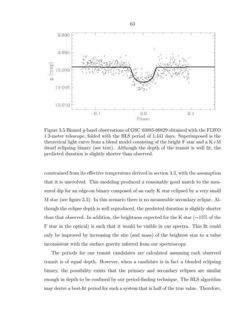
63

Figure 3.5 Binned g-band observations of GSC 03885-00829 obtained with the FLWO1.2-meter telescope, folded with the BLS period of 1.441 days. Superimposed is thetheoretical light curve from a blend model consisting of the bright F star and a K+Mdwarf eclipsing binary (see text). Although the depth of the transit is well fit, thepredicted duration is slightly shorter than observed.

constrained from its effective temperature derived in section 3.3, with the assumption

that it is unevolved. This modeling produced a reasonably good match to the mea-

sured dip for an edge-on binary composed of an early K star eclipsed by a very small

M star (see figure 3.5). In this scenario there is no measurable secondary eclipse. Al-

though the eclipse depth is well reproduced, the predicted duration is slightly shorter

than that observed. In addition, the brightness expected for the K star (∼15% of the

F star in the optical) is such that it would be visible in our spectra. This fit could

only be improved by increasing the size (and mass) of the brightest star to a value

inconsistent with the surface gravity inferred from our spectroscopy.

The periods for our transit candidates are calculated assuming each observed

transit is of equal depth. However, when a candidate is in fact a blended eclipsing

binary, the possibility exists that the primary and secondary eclipses are similar

enough in depth to be confused by our period-finding technique. The BLS algorithm

may derive a best-fit period for such a system that is half of the true value. Therefore,

64

Figure 3.6 TrES r-band photometry of GSC 03885-00829, folded using a period twicethat of our candidate planet (i.e., 2×1.441 days). (a) Best-fit blend model consistingof the bright F star and a pair of eclipsing K dwarfs (see text). The theoretical curveindicates a small difference in depth between the primary and secondary eclipse,(b) Enlargement around the primary eclipse, (c) Enlargement around the secondaryeclipse. The observed duration of the eclipses is well reproduced by the model.

65

we explored blend scenarios in which the period is 2 × 1.441 days. Figure 3.6 shows

the result of our best fit to the TrES r-band data, in which the eclipsing binary

is composed of two late K stars with masses of 0.67 and 0.64M⊙, with an orbital

inclination of 84◦ to the line of sight. The model indicates a slight difference in

eclipse depths (see figure 3.6a) of about 1 mmag, although this difference is only

marginally visible in observations themselves. Enlargements of the two eclipse regions

are displayed in the lower panels of figure 3.6. According to this fit, the time of the

center of transit previously derived (see Table 3.1) is, in fact, a time of secondary

eclipse; all of the photometric follow-up observations shown in figure 3.4 were taken

during a secondary eclipse. The brighter of the K stars (i.e., the primary of the

eclipsing binary) has only ∼3% of the light of the main F star in the optical, and is

below our threshold for spectroscopic detection. figure 3.2 shows the location of the

three stars (the filled circles) in the H-R diagram.

According to the blend model described above, the eclipse in the g band (a sec-

ondary eclipse) is predicted to be shallower than in the r band (0.35% versus 0.7%),

as we indeed observe, although the measured depth (0.4%) is slightly deeper than

that predicted. We attribute this to shortcomings in the isochrones used for the

blend modeling, which are not specifically designed for low-mass stars. In particu-

lar, missing opacity sources and other physical ingredients may affect the theoretical

luminosities in the optical (V or g) bands (Baraffe et al., 1998; Delfosse et al., 2000;

Chabrier et al., 2005), whereas the red and near-infrared magnitudes are presumably

more reliable. A sign of this is seen perhaps in the predicted V − K color for the

main F star: the isochrones give V −K = 1.26 (in the Johnson system as defined by

Bessell & Brett, 1988), bluer than the typical color of a dwarf of this temperature,

V −K = 1.40 (e.g., Bessell & Brett, 1988). Other stellar evolution models specifically

designed for low-mass stars such as those by Baraffe et al. (1998) appear to give more

realistic colors. Our F star is predicted to have V − K = 1.41 according to those

calculations (after transformation of the isochrone K magnitudes from the CIT to

the Johnson system, following Leggett, 1992), very close to the empirical value. Un-

fortunately the Baraffe et al. (1998) models are not publicly available for the Sloan

66

bands, so we are unable to use them in our blend modeling.

As indicated earlier, infrared magnitudes for GSC 03885-00829 are available from

the 2MASS Catalog. In particular, the measured V − K color of our candidate

in the Johnson system (Table 3.1) is 1.66 ± 0.02 (using transformations from the

2MASS system by Carpenter, 2001). The difference with the color of a single F star

indicates a significant infrared excess of about a quarter of a magnitude9. This in

itself can be taken as evidence of contamination from the light of a later-type object,

providing further evidence that we are dealing with a blend. The computed color

of the combined light of the three stars in our model using the Baraffe et al. (1998)

isochrones is V −K = 1.64, which agrees quite well with the observations and supports

our interpretation. Other predicted red and infrared colors also match the measured

values reasonably well (see figure 3.7).

Although it is quite possible that additional fine-tuning may improve the small

discrepancies noted above in the g band and provide a near-perfect fit to all obser-

vations (to the extent allowed by the accuracy of the stellar evolution models and

observational uncertainties), our goal here has been to show how subtle the signa-

tures of a blend can be, and that with careful modeling it is possible to demonstrate

that they are, in fact, due to a blend scenario and therefore reject the candidate.

3.6 Confirmation of Blend Model

In order to further test our blend hypothesis, we observed GSC 03885-00829 on

UT 2005 August 15 with the NIRSPEC infrared spectrograph at the Keck Observa-

tory. We observed the target in the K-band spectral region centered near 2.293µm,

to search for the presence of features from the 12CO 2–0 bandhead. Such features are

very weak for mid-G-type stars, and absent for stars with spectral types earlier than

G0. Hence, the detection of such features would indicate the presence of a cool stellar

photosphere, as predicted by our blend scenario.

9Hence, even if we underestimated the error in our V -band photometry (see section 3.4) by anorder of magnitude, the resulting propagation of error would not significantly affect the size of thisdiscrepancy.

67

Figure 3.7 Near-infrared colors measured for GSC 03885-00829 (dots) compared withthe theoretical colors of a single F star (dashed line) and the colors from our blendmodel (solid line; combined light of three stars). The latter is seen to reproduce theobserved colors well.

68

We used a 3-pixel-wide slit, which yields a spectral resolution of approximately

25,000. We gathered two 4-minute exposures, between which we nodded along the slit

by roughly 5′′. We differenced the two exposures to subtract the sky emission and any

pixel-dependent detector bias. We extracted the order spanning the location of the

12CO 2–0 bandhead by summing over a 15-pixel-wide band centered on the peak of

the instrumental profile. A small number of values in the extracted one-dimensional

spectrum were corrupted due to bad pixels in the infrared detector. We replaced

these values (30 of 1024 pixels) by interpolation. This region contains a large number

of telluric methane features. We produced a model of these features by modifying

the electronic version of the Kitt Peak National Observatory Fourier Transform Spec-

trometer (KPNO FTS) telluric spectrum (Livingston & Wallace, 1991) for air mass,

wavelength-solution, and instrumental PSF. Dividing our extracted spectrum by this

model yields the stellar spectrum corrected for telluric absorption.

In figure 3.8 we plot the resulting spectrum, as well as a spectrum of the nearby

M3V star GJ 725A (which shows very prominent CO features) for comparison. The

relative intensity between the individual CO features at 2.3µm does not differ for these

two types of stars, although the overall amplitude of the features is reduced for hotter

temperatures. We did not attempt to match the spectral type of the NIRSPEC data

quantitatively, since our primary goal is to exclude the planetary hypothesis. The

spectrum of GSC 03885-00829 clearly shows the 12CO 2–0 bandhead near 2.293µm;

the relative depth of the band head is approximately 6%. The detection of this feature

confirms the presence of a cool stellar photosphere. Also, for the late K dwarfs of

our model, the 12CO 2–0 band head has a depth of approximately 30%, and the K

dwarfs in our blend model contribute 25% of the K-band flux from the system. Hence

the expected depth of this band head in our spectrum is ∼7.5%, in rough agreement

with the observed relative depth. Thus, we interpret this feature as originating in the

photospheres of the K-stars of the binary.

The Heliocentric Julian day at mid-exposure was HJD 2453597.83591, which cor-

responds to an orbital phase of 0.09, at which point the expected velocity separation

between the two K stars is 89.5 km s−1. The K stars are likely tidally locked, and

69

Figure 3.8 K-band spectra of GSC 03885-00829 and a nearby M3V star (GJ 725A),obtained with the NIRSPEC spectrograph at the Keck Observatory. The M dwarfspectrum, with strong CO features, is shown for comparison with our target spectrum,which displays the 12CO 2–0 band head at approximately 2.293 µm. The spectrummust therefore include the light of a star with a spectral type later than the F-dwarftarget star, such as the K dwarfs of our blend model. The presence of the CO featurethus rules out the possibility of a planetary companion.

70

hence their spectral features will have a v sin i = 12 km s−1. Since this is smaller

than the predicted velocity separation at the time of the exposure, we might ex-

pect to resolve the individual components of the observed 12CO 2–0 feature from

the two K stars of the binary. And indeed the band head in our spectrum shows

two clear peaks of similar depth, with a velocity separation similar to the predicted

separation of the K dwarfs. A more careful analysis of this spectrum (e.g., using

the two-dimensional cross-correlation algorithm TODCOR; Zucker & Mazeh 1994)

should recover the components more precisely. However, for the purposes of this

paper, it is enough to identify the presence of the light from an eclipsing K binary

system in our spectrum, which rules out the transiting planet hypothesis.

3.7 The Necessity of Blend Identification

The difficult task of eliminating any contamination resulting in a false transit signal

is the primary challenge currently facing wide-field transit surveys. Developing this

experience will not only enable us to make firm detections of transiting Jupiters

but will be extremely valuable as we search for Earth-sized planets outside our solar

system with NASA’s Kepler mission. As with the ground-based wide-field surveys, the

challenge with Kepler will not only be obtaining the photometric precision necessary

to observe these minute signals, but rejecting all other possible causes of these eclipses

as well.

We have presented here one of our disappointments: a candidate that passed all

of our initial photometric and spectroscopic tests, but was later shown to be a result

of contaminated light from an eclipsing binary. As such, it highlights the difficulty in

rejecting all false positives from a transit survey. As the components of this eclipsing

binary are both faint K dwarfs, the resultant radial velocity variations in the light

blended with that from the nearby F star are not detectable. Also, the resultant color

dependence of the blended light curve is small, albeit observable, and the system

displays a color redder than that of an isolated F star.

The TrES survey readily produces on the order of 10 candidate transiting plan-

71

ets from each selected field of view with 15,000–25,000 stars, the majority of these

candidates proving to be astrophysical false positives. Some of these will mimic the

expected properties of a planetary system quite closely. On the basis of our expe-

rience of frequent blends, where the telltale indicators of the stellar components are

often masked, spectroscopic and even multicolor photometric follow-up is insufficient

to confirm the planetary nature of a candidate. An attempt must be made to inter-

pret the observations as those of a blended eclipsing binary and this interpretation

rejected only if the observations are not in agreement. Having meticulously examined

the evidence, we can commit to obtain the radial velocity orbit of this firm candidate

through high-resolution spectroscopy with a high signal-to-noise ratio. It should be

emphasized that determining the mass of the candidate from such observations is a

necessary step in identifying a transiting planet. The methods for rejecting astrophys-

ical false positives presented here and by other authors cannot be used to confirm the

planetary nature of a candidate; rather they increase the yield of planets from the

resource-intensive high-dispersion spectroscopy required for such a confirmation.

72

Chapter 4

TrES-2: The First TransitingPlanet in the Kepler Field1

Abstract

We announce the discovery of the second transiting hot Jupiter discovered by the

Trans-atlantic Exoplanet Survey. The planet, which we dub TrES-2, orbits the nearby

star GSC 03549-02811 every 2.47063 days. From high-resolution spectra, we deter-

mine that the star has Teff = 5960 ± 100 K and log g = 4.4 ± 0.2, implying a spectral

type of G0V and a mass of 1.08+0.11−0.05 M⊙. High-precision radial-velocity measurements

confirm a sinusoidal variation with the period and phase predicted by the photom-

etry, and rule out the presence of line-bisector variations that would indicate that

the spectroscopic orbit is spurious. We estimate a planetary mass of 1.28+0.09−0.04 MJup.

We model B, r, R, and I photometric timeseries of the 1.4%-deep transits and find

a planetary radius of 1.24+0.09−0.06 RJup. This planet lies within the field of view of the

NASA Kepler mission, ensuring that hundreds of upcoming transits will be monitored

with exquisite precision and permitting a host of unprecedented investigations.

4.1 The Search for Transiting Exoplanets

Observations of the 10 transiting hot Jupiters known at the time of writing have pro-

vided precise planetary radii and masses, and tested formation and structure models

1This chapter has been published previously as O’Donovan et al. 2006a, ApJL, 651, L61.

73

for extrasolar planets (see Laughlin et al., 2005; Charbonneau et al., 2007a). More

detailed studies of the nearby planets have probed their atmospheres and led to

the direct detection of their thermal emission (e.g., Charbonneau et al., 2002, 2005;

Deming et al., 2005a,b).

Three of these planets were known from radial-velocity surveys of the solar neigh-

borhood, and were subsequently observed to transit. The remaining seven were dis-

covered from photometric observations. The radial-velocity confirmation of transiting

planet candidates involves extensive use of large-aperture telescopes. With the goal

of maximizing the yield of transiting planets around bright stars and minimizing the

time required of large observatories, several teams are undertaking wide-field photo-

metric surveys using small telescopes (for a review, see Charbonneau et al., 2007a).

Our collaboration is conducting the Trans-atlantic Exoplanet Survey2 (TrES): TrES-1

was the first nearby transiting planet to be discovered photometrically (Alonso et al.,

2004a).

Such photometric surveys yield numerous transit candidates, of which the major-

ity are astrophysical false positives that are discarded by follow-up photometric and

spectroscopic observations (e.g., O’Donovan et al., 2007a, see chapter 2). However,

eliminating a blend, wherein a bright star forms a chance superposition or a hierar-

chical triple with a faint eclipsing binary, can require a careful analysis (Torres et al.,

2004b; Mandushev et al., 2005; O’Donovan et al., 2006b, see chapter 3).

We present here the discovery of the planet TrES-2 and describe the process by

which we confirmed its planetary nature and deduced its bulk properties.

4.2 Observations and Analysis of TrES-2

Transits of the parent star TrES-2 were first observed by Sleuth (Palomar Observatory,

California; O’Donovan et al. 2004) and the Planet Search Survey Telescope (PSST;

Lowell Observatory, Arizona; Dunham et al. 2004), part of the TrES network of ten-

centimeter telescopes. The third telescope, the Stellar Astrophysics and Research on

2See http://www.astro.caltech.edu/~ftod/tres/ .

74

Table 4.1. System parameters for TrES-2 planet

Parameter Value

P (days) 2.47063 ± 0.00001Tc (HJD) 2453957.6358 ± 0.0010a (AU) 0.0367+0.0012

−0.0005

i (deg) 83.90 ± 0.22K (m s−1) 181.3 ± 2.6Mp (MJup) 1.28+0.09

−0.04

Rp (RJup)a 1.24+0.09

−0.06

aHere RJup = 71,492 km, the equatorialradius of Jupiter at 1 bar.

Exoplanets (STARE; Alonso et al. 2004b) in Tenerife, Spain, did not observe because

it was undergoing an upgrade at the time. The two telescopes monitored a 5.7◦×5.7◦

field of view (FOV) centered on the star 16 Lyr from UT 2005 June 16 to September 3.

The analysis of TrES images has been described in detail in Dunham et al. (2004),

O’Donovan et al. (2006b, chapter 3), and O’Donovan et al. (2007a, chapter 2). In

summary, we analyzed the Sleuth and PSST images separately. After calibration,

we obtained a list of the field stars in each image and determined their equatorial

coordinates. We applied our image spatial interpolation and subtraction routines

based in part on Alard (2000) to obtain the differential magnitude of each star in

each image. We decorrelated and binned the stellar light curves, before applying

the transit-search algorithm of Kovacs, Zucker, & Mazeh (2002, see appendix C) to

identify stars showing statistically significant, periodic transit-like events.

We quickly selected TrES-2 as a prime candidate. The Sleuth r and PSST R pho-

tometric time series obtained near-transit and folded with a period P = 2.47063 days

are shown in figure 4.1. Five full transits and three partial transits were observed

by Sleuth. PSST observed two full transits and one partial event, events that were

also observed by Sleuth. We were therefore confident that the events were not the

result of instrumental error. The depth of 1.4% was consistent with the transit of a

75

Figure 4.1 Relative flux of the TrES-2 system as a function of time from the center oftransit, assuming the ephemeris in Table 4.1. The top light curve shows the unbinneddiscovery data, consisting of points from Sleuth r (filled diamonds) and PSST R(open diamonds). Each of the follow-up light curves is labeled with the telescope andfilter employed. We have overplotted the simultaneous best-fit solution, assuming theappropriate quadratic limb-darkening parameters for each band pass.

76

Table 4.2. System parameters for TrES-2 parent star

Parameter Value Reference

R.A. (J2000.0) 19h07m14.03s

Decl. (J2000.0) +49◦18′59.3′′

GSC 03549-02811Spectral Type G0V 1M⋆ (M⊙) 1.08+0.11

−0.05 1R⋆ (R⊙) 1.00+0.06

−0.04 1Teff (K) 5960 ± 100 1log g (dex) 4.4 ± 0.2 1v sin i (km s−1) 2.0 ± 1.5 1V (mag) 11.411 ± 0.005 1B − V (mag) 0.619 ± 0.009 1U − B (mag) 0.112 ± 0.012 1V − RC (mag) 0.361 ± 0.008 1J (mag) 10.232 ± 0.020 2J − H (mag) 0.312 ± 0.033 2J − Ks (mag) 0.386 ± 0.030 2[µα, µδ] (mas yr−1) [+4.45,−3.40] 3

References. — (1) This work; (2) 2MASS Catalog; (3)UCAC2 Bright Star Supplement.

Jupiter-sized object across a solar-type star, and the duration of only 1.5 hr implied

a near-grazing eclipse.

We searched for the counterpart of TrES-2 in publicly available catalogs and iden-

tified the star as GSC 03549-02811. The 2MASS J − Ks = 0.386 mag is consistent

with a Sun-like star. The UCAC2 proper motion (5.60 mas yr−1) is also consistent

with, but slightly less than, the expectation for a nearby dwarf. We examined the DSS

images and found no nearby bright companions within the 30′′ radius of the Sleuth

photometric aperture. In order to obtain absolute photometry and colors of TrES-2,

we observed it in Johnson UBV and Cousins R on the nights of UT 2006 August 29

and 30 with the 105-centimeter Hall telescope at Lowell Observatory. We calibrated

the data using six standard fields (Landolt, 1992), and the results are given in Ta-

77

ble 4.2.

We observed TrES-2 using the CfA Digital Speedometers (Latham, 1992) on UT

2005 October 18, 20, and 23, November 13, and 2006 June 13. These spectra are

centered on 5187 A and cover 45 A with a resolving power of λ/∆λ ≈ 35,000. By cross-

correlating these spectra with synthetic spectra created by J. Morse using Kurucz

model stellar atmospheres (J. Morse & R. L. Kurucz 2004, private communication),

we computed the radial velocity (RV) at each epoch. Within the measurement error

(∼0.5 km s−1), the RVs are constant with a mean velocity of −0.56 km s−1 and a

scatter of 0.55 km s−1. This limits the mass of the companion to be less than 8MJup.

From a similar cross-correlation analysis, we estimate (assuming a solar metallicity)

the stellar effective temperature Teff , surface gravity log g, and the projected rotational

velocity v sin i (Table 4.2). These estimates are consistent with the G0V spectral type

implied by the photometry.

We gathered rapid-cadence, high-precision photometric observations in I and B on

UT 2006 August 10 with the CCD camera at the IAC80, an 80-centimeter telescope

of the Observatorio del Teide, Tenerife, Spain. The CCD camera has a FOV of

10′ × 10′, corresponding to 0.′′33 pixel−1. After calibrating the images, we carried out

aperture photometry with vaphot (Deeg & Doyle, 2001) on the target and several

reference stars of similar brightness in the FOV. We constructed an ensemble average

of the calibrators, divided the target by the resulting time series, and renormalized the

resulting light curve by the median of its value prior to the transit event. Simultaneous

R observations were gathered with the TELAST 0.35-meter telescope, also located

at the Teide Observatory, and were analyzed in a similar fashion. This telescope is

able to follow the target to larger air mass permitting greater time coverage, but

the resulting light curve showed a residual trend that was likely due to an imperfect

extinction correction. To correct for this, we fit a cubic polynomial in time to the

out-of-transit data, extended the fit across the complete data set, and divided the

data by this function. For each data set, we estimated the measurement errors from

the rms variation of the data preceding first contact. The light curves are presented

in figure 4.1.

78

Table 4.3. Relative radial-velocity measurements of TrES-2

Observation Epoch Radial Velocity σRV

HJD - 2,400,000 m s−1 m s−1

53949.76054 135.5 6.153949.91993 96.8 6.153950.00216 58.9 7.753950.79018 −201.0 8.153950.93491 −204.8 9.053950.98051 −201.7 9.053951.02136 −198.5 7.253951.75032 91.7 6.053951.84863 136.7 7.053951.95209 140.5 7.153952.02736 145.6 8.4

In order to confirm the planetary nature of the companion and measure its mass,

we carried out RV observations using Keck/HIRES (Vogt et al., 1994) with its I2 ab-

sorption cell (Marcy & Butler, 1992). Eleven star + iodine spectra and one template

spectrum were collected on UT 2006 August 2–4, permitting good sampling of critical

orbital phases. We reduced the data using the MAKEE package written by T. Barlow.

Our spectra were gathered with a resolving power of λ/∆λ ≃ 71,000 and with expo-

sure times of 15 minutes, permitting a typical signal-to-noise ratio of 120 pixel−1. Our

analysis procedure to derive relative RVs incorporates the full modeling of temporal

and spatial variations of the HIRES instrumental profile (Valenti, Butler, & Marcy

1995; see also Butler et al. 1996; Korzennik et al. 2000; Cochran, Hatzes, & Paulson

2002). We model each echelle order containing I2 lines independently and then cal-

culate the internal uncertainties for this star for each observation as the RV scatter

about the mean divided by the square root of the number of spectral orders. The RV

precision achieved by our code is described in Alonso et al. (2004a) and Sozzetti et al.

(2006a,b). The RV measurements are listed in Table 4.3.

The best-fit orbital solution, constrained to have zero eccentricity (as expected

from theoretical arguments for a short-period planet), and with the P and transit

79

Figure 4.2 (Top) Radial-velocity observations of TrES-2 obtained with Keck/HIRESusing the I2 cell. The best-fit orbit (solid line) and γ-velocity (dashed line) areoverplotted. (Bottom) Residuals from the best-fit model to the radial-velocity data.

80

epoch Tc determined from the photometric data, yields a velocity semi-amplitude

K = 181.3± 2.6 m s−1 and an instrumental γ-velocity of γ = −29.8± 2.2 m s−1. The

fit has a χ2ν = 0.89 (ν = 9) and the rms of the residuals is 6.9 m s−1, in excellent

agreement with the internal errors. figure 4.2 shows the RV data overplotted with

the best-fit model, as well as the residuals to the fit. The parameters of the orbital

solution are listed in Table 4.1. We find a minimum mass for the planet of Mp sin i =

1.206± 0.016 (Mp+M⋆

M⊙ )2/3 MJup, where i is the orbital inclination and M⋆ is the stellar

mass. In section 4.3 we estimate these two quantities to obtain Mp. As a further

check on the consistency between the photometric and RV data sets, we fix P , set

e = 0, and solve for Tc (as well as K and γ). We find Tc = 2453957.6283 ± 0.0084,

which is consistent with, but less precisely determined than the value predicted from

the photometry (Table 4.1).

To investigate the possibility that the RV variations are due not to a planetary

companion but rather to distortions in the spectral line profiles arising from con-

tamination of the spectrum by an unresolved eclipsing binary (Santos et al., 2002;

Torres et al., 2005), we examined the line bisectors carefully for signs of time-varying

asymmetries. We cross-correlated each of our Keck spectra against a synthetic spec-

trum matching the measured properties of the star. Line bisectors were then com-

puted from the cross-correlation function averaged over spectral orders not affected by

the iodine lines, which is representative of the average spectral line profile. Bisector

spans were calculated as the velocity difference between points selected near the top

and bottom of the bisectors Torres et al. (2005). If the velocity variations were the

result of a stellar blend, we would expect the bisector spans to vary in phase with the

photometric period with an amplitude similar to that seen in the RVs (Queloz et al.,

2001; Mandushev et al., 2005). Instead, we did not detect any variation exceeding

the measurement uncertainties.

As an additional check we carried out detailed modeling of the TrES photometry

following Torres et al. (2004b) to test the hypothesis that the light curve is the result

of blending the main G0 star with an unseen eclipsing binary. The properties of the

three stars (parameterized in terms of their mass) were taken from model isochrones

81

subject to the Teff and log g constraints on the main star. An excellent fit to the TrES

r-band light curve was obtained for a triple system composed of a G-dwarf primary

blended with an eclipsing binary with individual components of spectral type M0

and M4–M5. In this model, the flux ratio between the G-dwarf primary and the

brightest (M0) component of the blended binary is less than 2%, which would be

undetectable in our spectra. However, the color difference between the G0 and M0

stars is such that we would expect the B data to present an eclipse depth half of that

in the TrES bandpass, in contrast to what is observed (figure 4.1). (Although we

note in section 4.3 that a modest color-dependent extinction error may be present in

the B data, it is both the opposite sign and of too small an amplitude to permit the

blend described here.) More generally, any blend scenario is strongly disfavored by

the observed RV orbit and corresponding lack of bisector variability.

We conclude from these tests that a blend scenario is strongly inconsistent with

the data, and therefore that the star is indeed orbited by a Jovian planet.

4.3 Estimates of Planet Parameters and

Conclusions

In order to determine M⋆ and its uncertainties, we compared our estimates of Teff and

log g with evolutionary models from Yi et al. (2001), assuming solar metallicity. For

each isochrone, we identified the range of M⋆ for which the Teff and log g lay within

our 1-σ errors. We took the best-fit model as our estimate of M⋆ and the span of

permitted models (over all ages greater than 500 Myr) to be our uncertainty. We then

used the resulting value, M⋆ = 1.08+0.11−0.05 M⊙, and the spectroscopic orbit (section 4.2)

to estimate Mp = 1.28+0.09−0.04 MJup. We also evaluated the stellar radius R⋆ in a simi-

lar fashion and found results that were consistent with, but less tightly constrained

than that from the light-curve modeling (below). The uncertainty contributed by

that in the evolutionary models is less than 0.02 M⊙. Based on the absolute visual

magnitude (MV =4.5) predicted by the best-fit model, we estimate the distance to be

82

approximately 230 pc. We estimate the reddening in the direction of TrES-2 to be

E(B−V ) ∼ 0.05 and the extinction to be ∼0.15 mag from comparison of its observed

colors with the intrinsic colors predicted by the model.

To estimate R⋆, i, and the planetary radius Rp, we simultaneously fit our light

curves using the analytical transit curves of Mandel & Agol (2002) and the color-

dependent quadratic limb-darkening parameters from Claret (2000) which were

matched to the spectroscopically estimated properties of the star. We identified

the best-fit solution by fixing the value of M⋆ at its best estimate, 1.08 M⊙, and

minimizing the χ2 to all the photometry. We note that the available time series are

well described by the model, with the exception of the IAC80 B, for which the in-

transit data fall below the model. We speculate that those data, which were gathered

at high air mass, may have been imperfectly corrected for extinction, which is a

larger effect at B than the other band passes. The best-fit solution obtains χ2ν = 1.15

(ν = 2065), and its values for {R⋆, Rp, i} are listed in Tables 4.1 and 4.2. The

uncertainties in these quantities are dominated by our uncertainty in M⋆. To derive

1-σ errors for each of {R⋆, Rp, i}, we change the value of that parameter and fix it at

a new value, and then allow the other two parameters to float, as well as allow for a

value of M⋆ within our uncertainty. (The uncertainties in P and Tc are sufficiently

small so as not to contribute significantly to the errors in R⋆, Rp, and i.) We repeat

this procedure until the best-fit solution produces an increase in the χ2 corresponding

to a 1-σ change. Our estimate of the planetary radius, Rp = 1.24+0.09−0.06 RJup, implies

a mean density of 0.83+0.12−0.09 g cm−3, indistinguishable from that of TrES-1 (using the

values from Sozzetti et al., 2004), despite the fact that TrES-2 is nearly twice as

massive. We also note that the impact parameter, b = a cos i/R⋆ = 0.84 ± 0.02, is

the largest of any known transiting exoplanet.

We intend to improve our estimates of the planetary and stellar parameters by

undertaking a more detailed analysis of the stellar spectrum as we did for TrES-1

(Sozzetti et al., 2004) and by gathering very high-precision z-band photometry (e.g.,

Holman et al., 2006). Such data will permit us to look for transit timing variations

indicative of additional planets in the TrES-2 system (Agol et al., 2005;

83

Holman & Murray, 2005; Steffen & Agol, 2005). TrES-2 lies within the FOV of the

NASA Kepler mission. During the four-year mission, Kepler will observe nearly

600 transits of TrES-2. The precision with which Kepler will observe these transits

will enable an extremely sensitive search for additional planets in the TrES-2 system

through their dynamical perturbations. Moreover, the large impact parameter means

that very subtle changes in its value could be detected. Such variations are pre-

dicted (Miralda-Escude, 2002) to occur as a result of either additional planets, or the

stellar quadrupole moment. Kepler may also detect the reflected light from TrES-2

(Jenkins & Doyle, 2003) and hence determine the long-sought geometric albedo and

phase function of a hot Jupiter. The large impact parameter also makes TrES-2 par-

ticularly favorable for determining the angle between the stellar spin-axis and the or-

bital axis via the Rossiter-McLaughlin effect (Gaudi & Winn, 2007). Williams et al.

(2006) discussed the use of Spitzer IRAC observations spanning the time of secondary

eclipse to resolve the surfaces of extrasolar planets. The large impact parameter of the

TrES-2 orbit is ideal for this application, since it grants access to both longitudinal

and latitudinal flux variations across the dayside hemisphere of the planet.

84

Chapter 5

TrES-3: A Nearby, Massive,Transiting Hot Jupiter in a31-Hour Orbit1

Abstract

We describe the discovery of a massive transiting hot Jupiter with a very-short

orbital period (1.30619 days), which we name TrES-3. From spectroscopy of the

host star GSC 03089-00929, we measure Teff = 5720 ± 150 K, log g = 4.6 ± 0.3, and

v sin i < 2 km s−1, and derive a stellar mass of 0.90 ± 0.15 M⊙. We estimate a plane-

tary mass of 1.92 ± 0.23 MJup, based on the sinusoidal variation of our high-precision

radial-velocity measurements. This variation has a period and phase consistent with

our transit photometry. Our spectra show no evidence of line bisector variations that

would indicate a blended eclipsing binary star. From detailed modeling of our B and z

photometry of the 2.5%-deep transits, we determine a stellar radius 0.802 ± 0.046 R⊙and a planetary radius 1.295 ± 0.081 RJup. TrES-3 has one of the shortest orbital per-

iods of the known transiting exoplanets, facilitating studies of orbital decay and mass

loss due to evaporation, and making it an excellent target for future studies of infrared

emission and reflected starlight.

1This chapter has been published previously as O’Donovan et al. 2007b, ApJL, 663, L37.

85

5.1 Transiting Exoplanets with Very-Short Orbital

Periods

The OGLE-III deep-field survey (Udalski et al., 2003, and references therein) has

identified three transiting planetary systems with very short orbital periods: OGLE-

TR-56b (P = 29 hr; Konacki et al. 2003), OGLE-TR-113b (P = 34 hr; Bouchy et al.

2004; Konacki et al. 2004), and OGLE-TR-132b (P = 41 hr; Bouchy et al. 2004). At

the time of discovery, such one-day-period planets were conspicuously absent from

radial-velocity (RV) surveys. These surveys had not discovered a planet with an

orbital period of substantially less than 3 days, despite the sensitivity of such sur-

veys to planets with short orbital periods. Several authors reconciled this appar-

ent discrepancy by determining the respective observational biases and selection ef-

fects (Gaudi, Seager, & Mallen-Ornelas, 2005; Pont et al., 2005; Gould et al., 2006;

Fressin et al., 2007). Since then, hot Jupiters with periods just over two days have

been detected by both RV surveys (HD 189733b; Bouchy et al. 2005b) and wide-field

transit surveys (WASP-2b; Collier Cameron et al., 2007), indicating a consistent pic-

ture for the underlying distribution of orbital periods of hot Jupiters.

With the discovery of these nearby planets, we continue to observe (Sozzetti et al.,

2007) the decreasing linear relation between P and the planetary mass (Mp) for tran-

siting planets first noticed by Mazeh, Zucker, & Pont (2005) and

Gaudi, Seager, & Mallen-Ornelas (2005). It appears from this small number of plan-

ets that shorter period exoplanets are on average more massive. This may suggest

different evolution of these planetary systems than the canonical migration (see, e.g.,

Trilling et al., 1998) of hot Jupiters from beyond the ice line.

We present here the discovery of TrES-3, a massive planet that has the one of the

shortest period of the transiting planets, and that was independently identified by

two transit surveys.

86

5.2 Observations and Analysis of TrES-3

Transits of the parent star GSC 03089-00929 were detected by two ten-centimeter

telescopes, part of the Trans-atlantic Exoplanet Survey (TrES) network. Sleuth (Palo-

mar Observatory, California; O’Donovan et al. 2004) observed seven full transits and

three partial transits, of which three full and two partial transits were observed by

the Planet Search Survey Telescope (Lowell Observatory, Arizona; Dunham et al.

2004). We obtained these observations between UT 2006 May 6 and 2006 Au-

gust 2, during which time we monitored a 5.◦7 × 5.◦7 field of view (FOV) centered

on θ Her. We then processed the data from each telescope separately, as we have

described previously (Dunham et al., 2004; O’Donovan et al., 2006b, see chapter 3;

O’Donovan et al., 2007a, see chapter 2). We then search our binned light curves us-

ing the box-fitting transit search algorithm of Kovacs, Zucker, & Mazeh (2002, see

appendix C) for periodic events consistent with the passage of a Jupiter-sized planet

across a solarlike star. We flagged TrES-3 as a candidate, noting that the transit

duration of 1.3 hr implied a high impact parameter b.

Transits of TrES-3 were independently observed by the Hungarian Automated

Telescope Network (HATNet; Bakos et al. 2004). We observed the HAT field “G196”

between UT 2005 June 8 and December 5, using the HAT-7 telescope at the Fred L.

Whipple Observatory (FLWO) and HAT-9 at the Submillimeter Array atop Mauna

Kea. We applied standard calibration and aperture photometry procedures to the

frames as described earlier in Bakos et al. (2007). We also applied the trend filtering

algorithm (Kovacs et al., 2005) and identified TrES-3 as a transit candidate using the

algorithm of Kovacs et al. (2002).

We observed TrES-3 using the CfA Digital Speedometers (Latham, 1992) on 13

occasions from 2006 September 9 to 2007 April 6. These spectra are centered at

5187 A and cover 45 A with a resolving power of λ/∆λ ≈ 35,000. We derived RVs at

each epoch by cross-correlation against synthetic spectra created by J. Morse using

Kurucz model stellar atmospheres (J. Morse & R. L. Kurucz 2004, private communi-

cation). There is no significant variation in these measurements, which have a mean

87

Table 5.1. TrES-3 parent star

Parameter Value Reference

R.A. (J2000.0) 17h52m07.03s

Decl. (J2000.0) +37◦32′46.1′′

GSC 03089-00929M⋆ (M⊙) 0.90 ± 0.15 1R⋆

a (R⊙) 0.802 ± 0.046 1Teff (K) 5720 ± 150 1log g (dex) 4.6 ± 0.3 1v sin i (km s−1) < 2 1V (mag) 12.402 ± 0.006 1B − V (mag) 0.712 ± 0.009 1V − RC (mag) 0.417 ± 0.010 1V − IC (mag) 0.799 ± 0.010 1J (mag) 11.015 ± 0.022 2J − H (mag) 0.360 ± 0.030 2J − Ks (mag) 0.407 ± 0.028 2[µα, µδ] (mas yr−1) [−22.5, +32.0] 3

References. — (1) This work; (2) 2MASS Catalog; (3)UCAC2 Bright Star Supplement.

aThe uncertainty in R⋆ includes both the statistical errorand the 5.6% uncertainty resulting from uncertainty in M⋆.

of +9.58 km s−1 and a scatter of 0.73 km s−1. This limits the mass of the companion

to be less than ∼7MJup. We estimated the stellar parameters from a cross-correlation

analysis similar to that above, assuming a solar metallicity. The effective temperature

(Teff), surface gravity (log g), and projected rotational velocity (v sin i) we derive are

listed in Table 5.1. On the basis of these values, we estimate the stellar mass to be

M⋆ = 0.90 ± 0.15 M⊙. Further spectroscopic analysis of the parent star (similar to

that performed for TrES-1 and TrES-2; Sozzetti et al. 2004, 2007) is in progress and

will be presented elsewhere.

The 2MASS J −Ks color (0.407 mag) and UCAC2 proper motion (39.1 mas yr−1)

of GSC 03089-00929 are as expected for a nearby G dwarf. We obtained absolute

88

Table 5.2. Relative radial-velocity measurements of TrES-3

Observation Epoch Radial Velocity σRV

HJD - 2,400,000 m s−1 m s−1

54186.99525 229.0 10.854187.11354 82.1 8.554187.96330 167.5 8.454188.04216 286.3 9.754188.96503 -336.5 8.654189.04672 -234.5 10.954189.09622 -183.9 9.3

BV RCIC photometry for TrES-3 on the night of UT 2007 April 14 with the 105-

centimeter Hall telescope at Lowell Observatory. The photometry was calibrated

using seven standard fields from Landolt (1992). The results are listed in Table 5.1.

We observed a full transit in the z band on UT 2007 March 26 using KeplerCam

(see, e.g., Holman et al., 2006) at the FLWO 1.2-meter telescope. We obtained 150,

90-s exposures of a 23.′1× 23.′1 FOV containing TrES-3. We observed another transit

in Bessell B on UT 2007 April 8 with the Las Cumbres Observatory Global Telescope

two-meter Faulkes Telescope North on Haleakala, Maui, Hawaii. The CCD camera

imaged a 4.6′ square field with an effective pixel size of 0.′′28 (the images were binned

2 × 2). We obtained 126 images with an exposure time of 60 s and a cadence of

70 s. We defocused the telescope slightly (to an image diameter of ∼3′′) to avoid

saturation of the brightest comparison star. We analyzed these data sets separately.

Using standard IRAF procedures, we corrected the images for bias, dark current, and

flat-field response. We determined fluxes of the target star and numerous comparison

stars using synthetic aperture photometry. To correct the target star fluxes for time-

varying atmospheric extinction, we divided them by a weighted average of the fluxes

of all the comparison stars.

We collected high-precision RV measurements on UT 2007 March 27–29 using

HIRES (Vogt et al., 1994) and its I2 absorption cell on the Keck I telescope. We ob-

89

Table 5.3. TrES-3 planet

Parameter Value

P (days) 1.30619 ± 0.00001Tc (HJD) 2454185.9101 ± 0.0003a/R⋆ 6.06 ± 0.10a (AU) 0.0226 ± 0.0013b = a cos i/R⋆ 0.8277 ± 0.0097i (deg) 82.15 ± 0.21K (m s−1) 378.4 ± 9.9γ (m s−1) −70.6 ± 6.2Mp (MJup) 1.92 ± 0.23Rp/R⋆ 0.1660 ± 0.0024Rp

a (RJup)b 1.295 ± 0.081

aThe uncertainty in Rp includes both thestatistical error and the 5.6% uncertainty re-sulting from uncertainty in M⋆ (Table 5.1).

bHere, RJup = 71,492 km, the equatorialradius of Jupiter at 1 bar.

tained a total of seven star+iodine exposures and one template spectrum. All spectra

were gathered with a nominal resolving power λ/∆λ ≃ 55 000, using the HIRES setup

with the 0.86′′ slit. We used an integration time of 15 minutes, which yielded a typical

signal-to-noise ratio of 110 pixel−1. We reduced the raw spectra using the MAKEE

software written by T. Barlow. We have described the software used to derive relative

radial velocities with an iodine cell in earlier works (e.g., O’Donovan et al., 2006a, see

chapter 4; Sozzetti et al., 2006a). We estimate our internal errors from the scatter

about the mean for each spectral order divided by the square root of the number of

orders containing I2 lines and find them to be around 10 m s−1. The radial-velocity

measurements are listed in Table 5.2.

We constrained the orbital fit to these data to have zero eccentricity (e), as ex-

pected from theoretical arguments for such a short-period planet, and we also held P

and the transit epoch Tc fixed at their values determined from the photometric data.

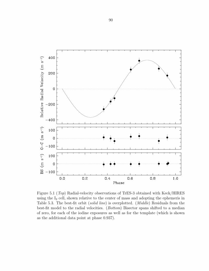
90

Figure 5.1 (Top) Radial-velocity observations of TrES-3 obtained with Keck/HIRESusing the I2 cell, shown relative to the center of mass and adopting the ephemeris inTable 5.3. The best-fit orbit (solid line) is overplotted. (Middle) Residuals from thebest-fit model to the radial velocities. (Bottom) Bisector spans shifted to a medianof zero, for each of the iodine exposures as well as for the template (which is shownas the additional data point at phase 0.937).

91

The rms residual from this fit (15.4 m s−1) is larger than the typical internal errors

(10 m s−1). Preliminary analysis of the template spectrum suggests that the star shows

evidence of activity. For the inferred spectral type, the presence of radial-velocity

“jitter” of 10–20 m s−1 is not unexpected (Saar, Butler, & Marcy, 1998; Santos et al.,

2000; Wright, 2005) and would explain the excess scatter we find. figure 5.1 displays

the RV data overplotted with the best-fit model, along with the residuals from the fit.

The parameters of the orbital solution are listed in Table 5.3. We find a minimum

planetary mass of Mp sin i = 2.035 ± 0.090[(Mp + M⋆)/M⊙]2/3MJup, where i repre-

sents the orbital inclination. As a consistency check we repeated the fit with P fixed

and e = 0 as before, but solving for Tc. The result is Tc = HJD 2,454,185.911 ± 0.045,

which is consistent with, but less precise than, the value determined from the pho-

tometry (Table 5.3).

We investigated the possibility that the velocity variations are due not to a plane-

tary companion but instead to distortions in the line profiles caused by an unresolved

eclipsing binary (Santos et al., 2002; Torres et al., 2005). We cross-correlated each

spectrum against a synthetic template matching the properties of the star and aver-

aged the correlation functions over all orders blueward of the region affected by the

iodine lines. From this representation of the average spectral line profile we com-

puted the mean bisectors, and as a measure of the line asymmetry we calculated the

“bisector spans” as the velocity difference between points selected near the top and

bottom of the mean bisectors (Torres et al., 2005). If the velocity variations were the

result of a stellar blend, we would expect the bisector spans to vary in phase with the

photometric period with an amplitude similar to that seen in the RVs (Queloz et al.,

2001; Mandushev et al., 2005). Instead, we do not detect any variation exceeding the

measurement uncertainties (see figure 5.1). We conclude that the RV variations are

real, and the star is indeed orbited by a Jovian planet.

92

5.3 Estimates of Planet Parameters and

Conclusions

We analyze our photometric time series using the analytic transit curves of

Mandel & Agol (2002) and the Markov Chain Monte Carlo (MCMC) techniques de-

scribed in Holman et al. (2006), Charbonneau et al. (2007b), and

Winn, Holman, & Roussanova (2007). We assume a circular orbit of constant P . We

first estimate Tc by fitting a model light curve (as described below) to only the z data.

We then determine P by phase-folding the z data with the TrES and HAT discovery

data (which affords a baseline of 1.8 yr) while varying the trial values for P . We then

fix the values for Tc and P (stated in Table 5.3) in the subsequent analysis.

The values of the planet radius Rp and the stellar radius R⋆ as constrained by the

light curves are covariant with M⋆. In our MCMC analysis, we fix M⋆ = 0.9 M⊙ and

then estimate the systematic error in the radii using the scaling relations Rp ∝ R⋆ ∝M

1/3⋆ (see Table 5.1, footnote a). We assume a quadratic limb-darkening law with

coefficients fixed at the band-dependent values tabulated in Claret (2000, 2004) for

the spectroscopically estimated Teff and log g and assuming solar metallicity.

The remaining free parameters in our model are Rp, R⋆, and i. We require two

additional parameters, kB and kz, the respective residual color-dependent extinc-

tion to the B and z light curves, assuming that the observed flux is proportional to

exp (−k m), where m denotes the air mass. We find that the TrES and HAT discovery

data are too noisy to meaningfully constrain the parameters, and so we restrict our

analysis to the B and z data. We first find the values of Rp, R⋆, i, kB, and kz that

minimize χ2 using the AMOEBA algorithm (Press et al., 1992). This model is shown

as the solid curves in figure 5.2. We then created two MCMC chains with 428,000

points each, one starting from the best-fit values and one starting from a randomly

generated perturbation to these values. We subsequently rejected the first 100,000

points to minimize the effect of the initial conditions, and found the results of the two

chains to be indistinguishable. We then examined the histograms of the five input

parameter values, as well as the histograms for several combinations of parameters

93

Figure 5.2 Relative flux of the TrES-3 system as a function of time from the centerof transit, adopting the ephemeris in Table 5.3, and including the residual color-dependent extinction correction (section 5.3). Each of these follow-up light curves islabeled with the telescope and filter employed. We have overplotted the simultaneousbest-fit solution, adopting the appropriate quadratic limb-darkening parameters foreach band pass.

94

relevant to anticipated follow-up studies. We assigned the optimal value to be the

median and the 1-σ error to be the symmetric range about the median that encom-

passed 68.3% of the values. We state our estimates of the parameters in Table 5.3.

The estimated values for kB (0.0029 ± 0.0006) and kz (−0.0021 ± 0.0004) are small

and of opposite sign, which is consistent with a modest difference between the average

color of the calibration field stars and the target.

Despite the V-shaped transit, our best-fit values indicate that TrES-3 is not graz-

ing, i.e., the disk of the planet is entirely contained within the disk of the star at

mid-transit, although grazing solutions are permitted by the data. Importantly, our

ability to obtain well-constrained estimates of Rp and R⋆ despite the large b hinged

on having observations of the transit in both B and z. The large difference in central

wavelength and hence stellar limb-darkening between these two bands permitted us

to rule out a family of degenerate solutions that is allowed by observations in only

a single color. We tested this notion by repeating the analysis above for only the z

data and found that values of Rp as large as 2.0 RJup could not be excluded.

TrES-3 presents a useful testbed for theoretical models of gas giants. Its radius

places it in the growing family of planets with radii that exceed that predicted for

models of irradiated gas giants. It is one of the most massive transiting planets and

has one of the the shortest periods. We recall that the discovery of OGLE-TR-56b at a

distance of only 0.023 AU from its star stimulated investigations into the timescales for

orbital decay and thermal evaporation. The comparable orbital separation of TrES-3

implies that many of these estimates are directly applicable to the new planet, but

with the important difference that the much brighter apparent magnitude affords the

opportunity for more precise study. In particular, we note that direct searches for

decay of the orbital period may inform our understanding of dissipation in stellar con-

vective zones (Sasselov, 2003), particularly since both the TrES-3 planet and its stellar

convective zone are more massive than that of OGLE-TR-56b. Furthermore, the mass

and orbital separation of TrES-3 are intriguingly close to the critical values estimated

by Baraffe et al. (2004), below which evaporation would become a dominant process.

The measurement of the angle between the planetary orbit and stellar spin axis of

95

TrES-3 may detect the substantial misalignment that might be expected for planets

that were tidally captured rather than migrating inward (Gaudi & Winn, 2007). As-

suming isotropic emission, the equilibrium temperature of TrES-3 is 1643(1−A)1/4 K,

where A is the Bond albedo. We intend to obtain Spitzer observations of TrES-3, as

we have previously done for TrES-1 and TrES-2. Finally, we note that TrES-3 is

extremely favorable for attempts to detect reflected starlight (Charbonneau et al.,

1999; Leigh et al., 2003; Rowe et al., 2006) and thus determine the geometric albedo,

pλ of the planet. The flux of the planet near opposition relative to that of the star

is pλ × (Rp/a)2 = pλ × 7.5 × 10−4, which is more than twice that of any of the other

known nearby transiting planets.

96

Chapter 6

Detection of Planetary Emissionfrom TrES-2 using Spitzer/IRAC

Abstract

With the discovery of nine new transiting planets within the last year, there have

been ample candidates for Target of Opportunity observations using the Spitzer Space

Telescope. We present here the results of the first of two planned series of observations

of TrES-2 using the Infrared Array Camera on Spitzer. TrES-2 is the most massive

such candidate to be observed with Spitzer. The brightness of this transiting system is

seen to decrease by 0.168 ± 0.022 % at 4.5µm, and 0.253 ± 0.045 % at 8.0µm, during

the secondary eclipse when the planetary emission is blocked by the star. We show

that these flux contrasts are well fit by a blackbody spectrum (similar to the results

from recent infrared observations of transiting hot Jupiters) with Teff = 1450 K, as well

as by a more detailed model spectrum with a planetary Teff of 1550 K and near-uniform

redistribution of the stellar insolation. The time of the center of the secondary eclipse

of TrES-2 is found to be consistent with predictions based on recent observations of

transits of TrES-2. This implies that TrES-2 mostly likely has a circular orbit, and

thus does not obtain additional thermal energy from tidal dissipation of a nonzero

orbital eccentricity.

97

6.1 Spitzer Observations of the Known Transiting

Exoplanets

There has been a recent dramatic increase in the number of nearby (d < 300 pc)

extrasolar planets whose structures and atmospheric compositions can be probed

using the Spitzer Space Telescope. These are the nearby transiting exoplanets (14 at

the time of writing, 10 of which were discovered in the last year). Spitzer observations

of these planets will help us understand the thermal dynamics associated with the

high insolation onto these planetary atmospheres, and thus how the radius of a hot

Jupiter varies with its mass.

Although over 200 extrasolar planets are known, it is only for these 14 nearby

transiting exoplanets that we can measure the planetary radius and true planetary

mass precisely enough to provide tight constraints for theoretical models. There have

been problems reconciling the observed planetary mass and radius with models (see

Laughlin et al., 2005; Charbonneau et al., 2007a, for a review). Several explanations

have been proposed for the bloated planets, mainly regarding some additional source

of energy combating planetary contraction (see, e.g., Guillot & Showman, 2002).

Deming et al. (2005b) refuted the possibility that tidal damping of a nonzero eccen-

tricity was one such energy source for HD 209458b (Bodenheimer, Lin, & Mardling,

2001; Bodenheimer, Laughlin, & Lin, 2003). By measuring the timing of the sec-

ondary eclipse of HD 209458b, they showed that the planetary orbit is circular, as

expected for a hot Jupiter, unless it is gravitationally affected by an unseen planetary

companion (see, e.g., Rasio & Ford, 1996). In order to fully understand these inflated

radii, we have begun to estimate the atmospheric composition of the nearby exo-

planets (for a discussion of extrasolar planetary atmospheres, see Charbonneau et al.,

2007a; Marley et al., 2007). Detection of emission from planetary atmospheres was

made possible by taking advantage of the enhanced contrast between stars and their

planets in the infrared. Infrared emission has been detected from HD 209458b and

HD 189733b, both at specific wavelengths (Deming et al., 2005b, 2006), and over

a wide spectral range (Richardson et al., 2007; Swain et al., 2007; Grillmair et al.,

98

2007). Charbonneau et al. (2005) also reported infrared emission from TrES-1. There

has been a flurry of activity to reconcile atmospheric models with this limited num-

ber of infrared measurements. While several attempts have been made to explain the

infrared observations (see, e.g., Barman et al., 2005; Burrows, Hubeny, & Sudarsky,

2005; Burrows et al., 2007; Fortney et al., 2005; Fortney et al., 2006a; Seager et al.,

2005), the models are not entirely in agreement and no single model can explain ev-

ery observation. There is a clear need to obtain as many additional observations of

extrasolar planetary atmospheres as possible during Spitzer’s limited lifetime.

The transiting hot Jupiter TrES-2 (O’Donovan et al., 2006a, see chapter 4) is

the most massive of the transiting systems that has been followed up with Spitzer,

providing a key constraint for our understanding of the gas giant mass-radius relation.

Here we present the first Spitzer observations of TrES-2 (section 6.2). From our

analysis (section 6.3), we have detected thermal emission from the transiting planet,

and compared our results with various atmospheric models (section 6.4).

6.2 IRAC Observations of TrES-2

In a similar manner to the previous Spitzer observations of TrES-1 (Charbonneau et al.,

2005), we employed two of the four bandpasses available on the Infrared Array Cam-

era (IRAC; Fazio et al. 2004) on Spitzer to monitor TrES-2 during the time of sec-

ondary eclipse. We selected the 4.5-µm and 8.0-µm channels; future observations

of TrES-2 at 3.6µm and 5.8µm are planned. We took care to position TrES-2

(2MASS J19071403+4918590: J = 10.232 mag, J − Ks = 0.386 mag) away from ar-

ray regions impaired by bad pixels or scattered light. We also kept the corresponding

IRAC stray light avoidance zones free of stars that are bright in the infrared. We ob-

served a 5.′2 × 5.′2 field of view (FOV) containing TrES-2 for 3.9 hr on UT 2006 Novem-

ber 30 (starting at HJD 2,454,069.956), and obtained 1073 images in both channels

with an effective integration time of 10.4 s.

99

6.3 Deriving and Modeling Light Curves of

TrES-2

As part of the standard pipeline for IRAC data, the images are dark current sub-

tracted, flat-fielded, and corrected for any detector nonlinearity. Each header of

these Basic Calibrated Data (BCD) images contains the time and date of observation

and the effective integration time. We used these to compute the Julian date cor-

responding to mid-exposure of each observation. In order to convert these dates to

Heliocentric Julian dates, we subtracted 30.926 s from each to account for the light

travel time between the Sun and Spitzer. We then computed the orbital phases us-

ing the orbital period (P = 2.47063 ± 0.00001 days) from O’Donovan et al. (2006a,

see chapter 4) and an updated transit epoch (TC = HJD 2,454,041.63598 ± 0.00030;

Holman et al. 2007b) derived from recent observations made as part of the Transit

Light Curve project.

Using an initial estimate of the position of TrES-2 on the array, we computed the

arithmetic centroid of TrES-2 in each BCD image. We then measured the flux from

our target using circular apertures ranging from 2 to 10 pixels, and sky subtracted

using a sky annulus with inner and outer radii of 20 and 30 pixels, respectively. We

normalized the fluxes for a given channel and aperture size using the corresponding

median flux value. We examined the variation of the rms of the out-of-eclipse data,

and found that an aperture size of 3 pixels produced the smallest rms for both chan-

nels. We then performed a separate analysis of these two light curves from the two

channels, as IRAC displays different characteristics at 4.5µm and 8.0µm.

The 8.0-µm data showed an overall increase in flux with time, but the first 32

minutes of data displayed a steeper slope. We excluded this initial data and large

flux outliers from further analysis. In order to remove the trend, we computed a linear

fit to the out-of-eclipse data, and then divided the data set by this model. In order

to extract the depth and epoch of the secondary eclipse, we created a model using

the eclipse light curve code for a uniform source from Mandel & Agol (2002), allow-

ing the eclipse depth (∆f8.0) and the offset (∆t8.0) from the predicted eclipse epoch

100

Figure 6.1 Relative fluxes from the TrES-2 system at 8.0µm (bottom) and at 4.5µm(top, with an arbitrary flux offset), binned and plotted versus the time from the pre-dicted center of secondary eclipse (Ts). Superimposed are our best-fit models (blacklines) with depths of ∆f4.5 = 0.00168 ± 0.00022 and ∆f8.0 = 0.00253 ± 0.00045, re-spectively. The timing of the secondary eclipse was allowed to vary for the 8.0-µm data(but not for the 4.5-µm data), and the derived timing offset (∆t8.0 = −3.6+5.8

−4.4 minutes)is consistent with eclipse occurring at the predicted Ts. The dotted line represents amodel with the same depth as our best-fit model of the 8.0-µm data, but with zerotiming offset.

101

(HJD 2,454,070.04823 ± 0.00030) to vary. The required system parameters were the

planetary orbital period, impact parameter and orbital inclination (P = 2.47063 days,

b = 0.84; O’Donovan et al. 2006a [see chapter 4], and i = 83.9◦ Holman et al. 2007b),

and the radius ratio between the planet and the star (Rp/R⋆ = 0.1251; Holman et al.

2007b). For each pair (∆f8.0, ∆t8.0) over the range (0.0005 ≤ ∆f8.0 ≤ 0.0040, −40

minutes ≤ ∆t8.0 ≤ 40 minutes), we computed the χ2 of the corresponding model to

the 8.0-µm data, again excluding large flux outliers. The best-fit values were an eclipse

depth of ∆f8.0 = 0.00253 ± 0.00045 and a timing offset of ∆t8.0 = −3.6+5.8−4.4 minutes,

where the negative sign in time corresponds to an early secondary eclipse. Thus we

see that the best-fit timing offset is consistent with the predicted epoch for the sec-

ondary eclipse. figure 6.1 shows this best-fit model, superimposed with the 8.0-µm

data binned using 7-minute bins. The reduced χ2 for this fit was:

χ2r = χ2/(N − 2),

= 857.4/(852 − 2),

= 1.01,

corresponding to a well-fit data set.

An upper limit for the orbital eccentricity of a transiting planet can be com-

puted from the timing offset ∆t8.0 derived above, using e cos ω ≃ π ∆t8.0/2 P , where

ω is the unknown longitude of periastron and P is the known orbital period (see

equation 4 of Charbonneau et al., 2005). This upper limit for TrES-2 is there-

fore 0.00145 ± 0.00096, consistent with a negligible orbital eccentricity. Spitzer has

also obtained a negligible orbital eccentricity for two other planets: HD 209458b

(Deming et al., 2005b) and TrES-1 (Charbonneau et al., 2005). Tidal damping of

orbital eccentricity (Bodenheimer, Lin, & Mardling, 2001;

Bodenheimer, Laughlin, & Lin, 2003 has yet to be shown to be a sizable contribution

to the internal energy of any exoplanet.

The analysis of the 4.5-µm data was complicated by the known correlation between

the IRAC 4.5-µm flux from a source and the intra-pixel position on the detector. For

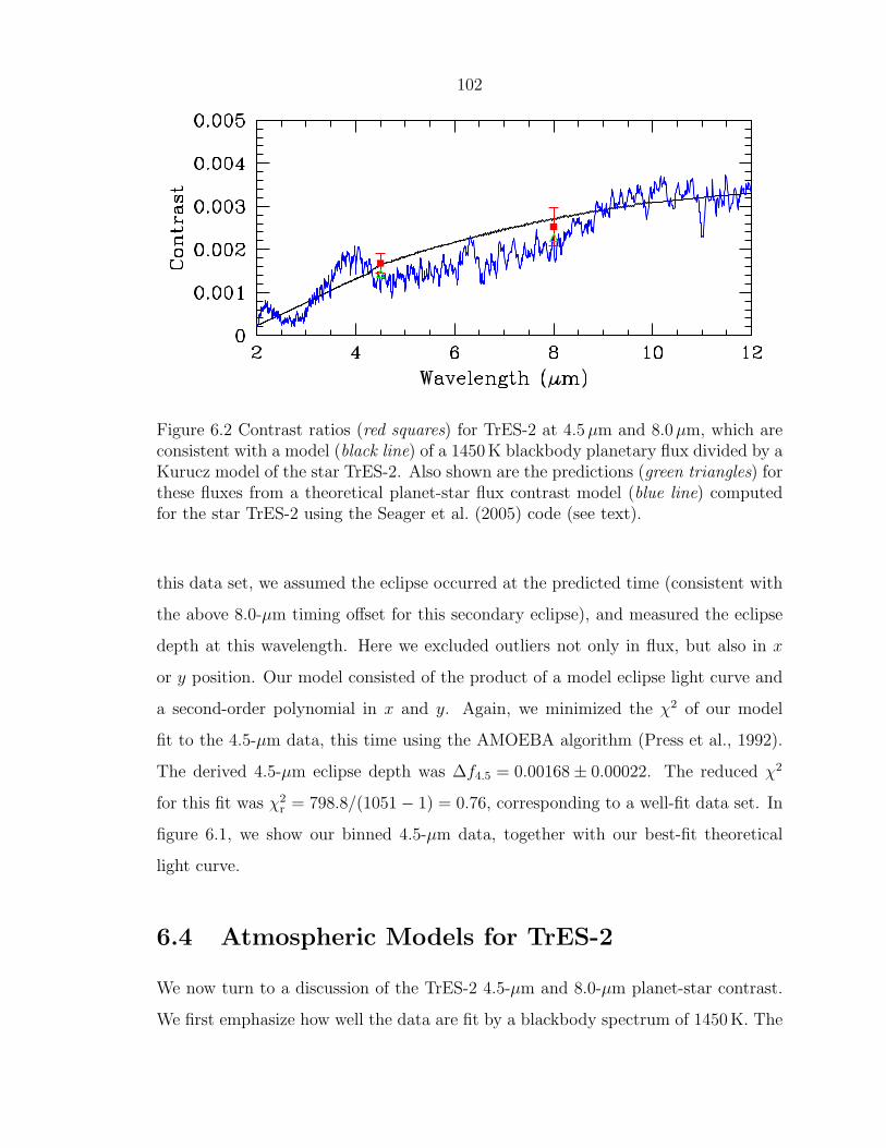
102

Figure 6.2 Contrast ratios (red squares) for TrES-2 at 4.5µm and 8.0µm, which areconsistent with a model (black line) of a 1450 K blackbody planetary flux divided by aKurucz model of the star TrES-2. Also shown are the predictions (green triangles) forthese fluxes from a theoretical planet-star flux contrast model (blue line) computedfor the star TrES-2 using the Seager et al. (2005) code (see text).

this data set, we assumed the eclipse occurred at the predicted time (consistent with

the above 8.0-µm timing offset for this secondary eclipse), and measured the eclipse

depth at this wavelength. Here we excluded outliers not only in flux, but also in x

or y position. Our model consisted of the product of a model eclipse light curve and

a second-order polynomial in x and y. Again, we minimized the χ2 of our model

fit to the 4.5-µm data, this time using the AMOEBA algorithm (Press et al., 1992).

The derived 4.5-µm eclipse depth was ∆f4.5 = 0.00168 ± 0.00022. The reduced χ2

for this fit was χ2r = 798.8/(1051 − 1) = 0.76, corresponding to a well-fit data set. In

figure 6.1, we show our binned 4.5-µm data, together with our best-fit theoretical

light curve.

6.4 Atmospheric Models for TrES-2

We now turn to a discussion of the TrES-2 4.5-µm and 8.0-µm planet-star contrast.

We first emphasize how well the data are fit by a blackbody spectrum of 1450 K. The

103

black line in figure 6.2 is a 1450 K blackbody flux divided by a Kurucz stellar model

appropriate for the stellar parameters derived by Sozzetti et al. (2007). A blackbody

of 1450 K implies a Bond albedo of 0.12, with the assumption of uniform redistribution

of absorbed stellar radiation. If TrES-2 is indeed a blackbody, it would add to the

growing list of published hot Jupiter atmosphere data commensurate with blackbody

spectra, showing no evidence for the atmospheric composition. These exoplanets

include two of the three exoplanets with more than one published data point: TrES-1

(Charbonneau et al., 2005) and the HD 189733b spectrum (Grillmair et al., 2007). A

theoretical planet-star flux contrast that fits the data is also shown as the blue line

in figure 6.2. The TrES-2 spectrum was generated from a model atmosphere code for

hot Jupiters (Seager et al., 2005) with inputs appropriate to the TrES-2 planet-star

parameters, solar abundances, and a Kurucz model atmosphere for the irradiation

from the parent star. We reduce the incident stellar flux by f = 0.9 to take into

account the redistribiution of absorbed stellar radiation. This value is intermediate

between the values for instantaneous reradiation (f = 3/8) and uniform redistribution

(f = 1) of absorbed stellar radiation. The planet spectrum has Teff = 1550 K. Planets

with higher values of f (i.e., under the assumption that the absorbed stellar radiation

is redistributed more uniformly) than the one we chose have flux values too low in

both the 4.5-µm and 8.0-µm bandpasses. We justify our somewhat arbitrary choice

of f based on the results of Fortney et al. (2006a) that 1-D models do not represent

the 3-D dayside temperature pressure profiles that likely result from a highly complex

atmospheric circulation.

6.5 Searching for Evidence of Atmospheric

Absorption

The Spitzer data we report for TrES-2 is markedly different than for TrES-1

(Charbonneau et al., 2005). In comparing the TrES-2 and TrES-1 data sets with

each other and with models, it is useful to define a Spitzer IRAC color index: the

104

ratio of the 8.0-µm to 4.5-µm planet-star flux contrast. For TrES-1 the color in-

dex is 3.41 ± 0.87. This ratio was too high to fit most atmosphere models in the

literature (see Fortney et al., 2005; Seager et al., 2005; Barman et al., 2005; but cf

Burrows, Sudarsky, & Hubeny 2006). Although many different models (including

such effects as high metallicity, energy deposition at high alitudes in the atmosphere;

varying C/O ratios, energy redistribution parametrizations) have since been explored

(Barman et al., 2005; Fortney et al., 2005; Seager et al., 2005;

Burrows, Sudarsky, & Hubeny, 2006), none reach the TrES-1 value of 3.4.

TrES-2 has a much lower color index (1.51 ± 0.33) than TrES-1. This value is much

more easily fit by “generic” hot Jupiter atmosphere models. Indeed, a wide variety of

theoretical models with solar abundances, with uniform or hemispheric redistribution,

with or without clouds, and for a wide range of temperatures and redistribution

values, have ratios consistent with the TrES-2 color index (see, e.g., Fortney et al.,

2005; Barman et al., 2005; Charbonneau et al., 2005). This is primarily because the

water vapor absorption features in these models dominate the spectra, and appears

to create a somewhat consistent color index.

Spitzer IRAC data at 3.6µm and 5.8µm are forthcoming for TrES-2. These

additional data are critical to distinguish between a blackbody spectrum, a radiative

equilibrium solar abundance spectrum, and other atmosphere models.

105

Chapter 7

Identifying Transits inTrES Data Sets:The Human Factor

7.1 Understanding the Yield of Transit Surveys

The discovery of the first transiting planet HD 209458b (Charbonneau et al., 2000;

Henry et al., 2000) spawned a great flurry of campaigns to search for these rare ob-

jects. Transiting planets yield precise measurements of the radius and mass of giant

planets outside our solar system that are much needed constraints for theoretical

models, and they provide the promise of a better understanding of the structure and

formation of gas giants. HD 209458b was first identified (Mazeh et al., 2000) as a

Jupiter-mass planet by radial-velocity surveys of the solar neighborhood. It was later

observed to transit its star. In comparison, the majority of transit surveys aimed to

photometrically monitor 100,000s of stars for evidence of transits. Initial estimates

(see, e.g., Horne, 2003) of the yield of transiting planets from these surveys were opti-

mistic during the initial rush of enthusiasm, with expectations of many new discoveries

every month. At the time of writing, seven years later, there are only 20 known tran-

siting exoplanets. Several transit surveys have overcome the difficulty in obtaining

the photometric precision required to observe a 1% transit over a large field of view for

thousands of stars, and have proven their ability to identify transiting planets: the

OGLE-III survey (Udalski et al., 2002), the XO project (McCullough et al., 2005),

106

the HAT survey (Bakos et al., 2002), the SuperWASP survey (Street et al., 2003),

and the Trans-atlantic Exoplanet Survey (TrES; Alonso et al. 2004b; Dunham et al.

2004; O’Donovan et al. 2004). Despite these successes, the anticipated flood of new

transiting planets is still only a trickle.

Over time, we have developed a greater appreciation of additional factors that

must be included in our predictions (see Gaudi, 2007, for a review): (i) Transit

surveys are very biased toward large planets with short periods

(Gaudi, Seager, & Mallen-Ornelas, 2005; Gaudi, 2005). (ii) Many of the stars in a

given field are giants or large dwarfs (Brown, 2003); hence transits of these large stars

are not detectable by ground-based surveys with ten-centimeter telescopes. (iii) The

presence of systematics in the data, correlated on transit-like time scales, increases

the signal-to-noise ratio requirement to detect a transit to beyond that derived from

simple Poisson noise. This increases the number of observed transits required to have

a strong transit detection, and hence affects the choice of the length of the observing

run for the field.

These factors affect the number of strong transit signals that are expected in the

data. However, when estimating the yield from a survey, we must account for how

we detect these periodic signals. There are two steps in my procedure for identify-

ing candidate transiting systems. First, I use an automated algorithm to find the

statistically most significant transit signals. Then, I view these strong signals and

determine which are worth further analysis. It is important that both steps are ef-

ficient in recovering transit signals. Several algorithms have been proposed in the

case of transit surveys (see, e.g., Tingley, 2003a,b, for a review). For the analysis of

the TrES data, I use the Box-fitting Least-Squares (BLS) transit-search algorithm of

Kovacs, Zucker, & Mazeh (2002, see appendix C), as do several other groups such as

the HAT survey. Several studies of the potential recovery rates of transit candidates

have been done by transit surveys (see, e.g., Gilliland et al., 2000; Bramich et al.,

2005; Kane et al., 2005; Weldrake & Sackett, 2005). Here I present the recovery rate

of the BLS algorithm when applied to TrES data. I also discuss my ability to spot true

transit signals among the noise, as the efficiency of this step has not been previously

107

Figure 7.1 Histogram of the 2MASS J − Ks infrared colors for the TrES Lyr1 field.

quantified.

7.2 Injecting Model Light Curves into a

TrES Data Set

I conducted a blind test of my ability to identify transit-like signals in a real data set

from the TrES campaign. I chose the TrES Lyr1 field (centered on the star 16 Lyr)

in which I had identified the transiting planet TrES-2 (O’Donovan et al., 2006a, see

chapter 4). The total yield to date of this 5.7◦ × 5.7◦ field, which contains 27,446

stars, is one confirmed planet.

First I generated a list of parameters for fake transit light curves as follows. Note

that I did not consult this parameter list until I had attempted to visually identify

108

Figure 7.2 Randomized stellar parameters used to generate fake transit light curvesinjected into a TrES time series, plotted versus the approximate VT magnitudes: (toppanel) the mass of the host star, and (bottom panel) the stellar radius. The numberof stars of a given magnitude increases with magnitude. The stellar mass and radiuswere generated using the 2MASS J − Ks infrared colors from figure 7.1 (see text fora discussion of the distribution). These values were computed to two decimal places,which results in the discrete levels visible in the plots.

109

Figure 7.3 Same as for figure 7.2, but for the radius Rp of the supposed transitingplanet. Again, the discrete levels in the values for Rp are due to the limit of twodecimal places for the values.

110

all of the fake candidate transiting planets. As part of the standard TrES analy-

sis pipeline (see, e.g., Dunham et al., 2004; O’Donovan et al., 2006b, see chapter 3;

O’Donovan et al., 2007a, see chapter 2). I had previously generated a list of 27,446

stars present in the Lyr1 field, ordered by instrumental r magnitude. The position

of a star in this list, starting at 0 for the brightest star, is the “star number” for this

star. In order to span a wide range of transit parameters, I would need to inject a

large number of fake transits. However, I would also need to somewhat simulate the

scarcity of real transit signals in the data. I decided to choose a random1 number of

fake transits to be injected, such that this number was ∼10% of the total number of

stars. I then chose this number (2,612) of stars at random from the star list to be the

ostensible candidate hosts of transiting planets. From the 2MASS (Cutri et al., 2003)

J − Ks infrared colors of these stars (see figure 7.1), I derived the stellar masses M⋆

and radii R⋆, assuming these to be dwarf stars and using an interpolation2 of values

from Cox (2000). Note that since most of the stars with large J − Ks values are

in fact giants, the assumption that these stars are main-sequence stars (with small

stellar radii corresponding to their color) leads to a bias towards identifying transiting

planets that are too small to be detected if transiting giant stars. The scarcity of radii

R⋆ < 0.65 R⊙ and R⋆ > 1.40 R⊙ (and the similar dearth in masses) is the result of

the 2MASS color distribution of figure 7.1. I produced a random distribution of radii

Rp for the supposed planetary companions of these stars, where 0.9 ≤ Rp ≤ 1.2 RJup

based on the distribution of radii for the known transiting planets (see figure 1.3).

The values for these three physical parameters are shown in Figures 7.2 and 7.3.

I then computed random values for the transit impact parameter b (0 ≤ b ≤ 1).

The orbital inclination i can be derived from b using i = arccos (bR⋆/a), where a

is the orbital semi-major axis computed using Newton’s revised version of Kepler’s

1The random numbers discussed in this chapter were generated using IDL’s RANDOMU functionthat generates uniformly distributed, pseudo-random numbers using the method of Park & Miller(1988).

2The gaps in the stellar masses and radii were caused by a bug in the interpolation code thatwas not discovered until the hidden parameter file was examined after the analysis. Future analysiswill correct this. However, I decided that the stellar radii (the more interesting parameter) cover awide enough parameter space for my initial analysis.

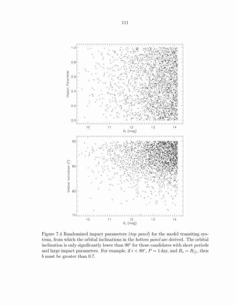
111

Figure 7.4 Randomized impact parameters (top panel) for the model transiting sys-tems, from which the orbital inclinations in the bottom panel are derived. The orbitalinclination is only significantly lower than 90◦ for those candidates with short periodsand large impact parameters. For example, if i < 80◦, P = 1 day, and R⋆ = R⊙, thenb must be greater than 0.7.

112

third law. The distribution of b and i can be seen in figure 7.4.

The BLS transit-search algorithm computes four transit parameters for every in-

put light curve: the orbital period P of the transit, the depth ∆, the fractional

duration d = D/P (where D is the duration), and the orbital phase Φ at the time

Tc of the transit center. I generated random values for P (1 ≤ P ≤ 5 days; again see

figure 1.3) and Φ (0 ≤ Φ ≤ 1). Note that while Φ is normally defined so that Φ = 0

at Tc, here Φ is defined so that Φ = 0 at the start of the TrES observing run. This is

to conform with the definition used by our BLS algorithm for Tc. I derived the transit

depths from ∆ = (Rp/Rstar)2, and the fractional transit durations using equation 4

from Charbonneau et al. (2006):

sin i cos

(

πD

P

)

=

√

1 −(

R⋆ + Rp

a

)2

,

i ∼ 90◦ ⇒ d =1

πarccos

√

1 −(

R⋆ + Rp

a

)2

.

Figures 7.5 and 7.6 shows the distribution of the parameters that should be recovered

by the BLS algorithm.

Using these random system parameters as unseen input, I generated model transit

light curves using code based on the analytic formulae of Mandel & Agol (2002).

This code computes the variation with time in the amount of obscuration of a limb-

darkened source by a dark body, by deriving the area of the source obscured at

that time, and outputs this variation in terms of relative flux. Although the TrES

photometry is too noisy to discern between different limb-darkening due to different

stellar spectral types, the code requires limb-darkening coefficients as part of the

input. I assumed a quadratic limb-darkening model of the form:

I(µ)/I(1) = 1 − a(1 − µ) − b(1 − µ)2,

where µ = cos γ, γ is the angle between the line of sight and the local normal to

the stellar surface, I is the specific intensity, and a and b are the limb-darkening

113

Figure 7.5 Randomized values for two of the four parameters that are derived foreach light curve by the Box-fitting Least-Squares (BLS) transit-search algorithm:(top panel) the orbital period P of the transit, and (bottom panel) the transit depth∆. To mimic the output of the BLS algorithm, P and ∆ are kept to 6 and 3 decimalplaces, respectively. Since 0.9 RJup ≤ rp ≤ 1.2 RJup and most derived stellar radiilie in the range 0.7 R⊙ ≤ R⋆ ≤ 1.3 R⊙, most of the transit depths are in the range0.005 ≤ ∆ ≤ 0.03. The outliers are those transits of a very small star by very largeplanet, or of a very large star by a very small planet. These points are evidence ofthe aforementioned bias caused by the assumption that all field stars are dwarf stars.

114

Figure 7.6 Same as for figure 7.5, but for (top panel) the fractional transit duration d,and (bottom panel) the orbital phase Φ at the time of transit. To mimic the outputof the BLS algorithm, d and Φ are kept to 3 decimal places. The fractional transitduration is only significantly higher than 0.06 for those candidates with short periodsand small stellar radii. For example, if d = 0.1, then a must be approximately 3R⋆.

115

Figure 7.7 (Top) Model transit light curves for a 1.2% transit with a period of1.038588 days. The shape of the three light curves is determined by the limb-darkeningassociated with the specified spectral type. Distinguishing between these light curvesis not possible for the TrES photometry, hence I simply assumed the G0V limb-darkening coefficients. (Bottom) Model transit light curve from the top panel plottedversus the times of observation during the TrES Lyr-1 run.

116

Figure 7.8 The top light curve is from the TrES Lyr1 field, phased to an orbitalperiod of 1.038588 days. The bottom light curve shows the results of injecting themodel transits from figure 7.7.

117

coefficients. The R-band quadratic limb-darkening coefficients for a G0V star (a

typical spectral type from my data; see figure 7.1) are a = 0.2938 and b = 0.3441

(Teff = 6000 K, log g = 4, [Fe/H]=0, Vturb = 0 km s−1; Claret 2000). figure 7.7 shows a

phased model light curve using these coefficients and assuming Rp/R⋆ = 0.1. figure 7.7

also shows model light curves displaying limb-darkening associated with a K5V and

F0V star. Distinguishing between the different limb-darkening requires photometry

with exquisite precision (such as seen in Brown et al. 2001). I simply assumed a G0V

spectral type and luminosity class for my analysis.

I then accounted for the actual temporal coverage of the observations. The effect

of this can be seen in the bottom panel of figure 7.7, where the model from the top

panel have been plotted versus the times of observation of the Lyr1 field. The final

product of the TrES pipeline is a series of light curves, one for each star in the field.

These light curves have been decorrelated to remove systematics suffered by wide-field

transit surveys, and averaged (in 9-minute bins) to reduce the computational effort of

the BLS transit search. For this test, I chose the combined binned TrES data set, with

observations from both Sleuth3 (Palomar Observatory, California; O’Donovan et al.

2004) and the Planet Search Survey Telescope (PSST; Lowell Observatory, Arizona;

Dunham et al. 2004). Since these TrES time series and model light curves both

have units of magnitudes, I added to the time series for each fake host star the

corresponding model light curve to produce the fake time series. The light curves of

the stars not chosen as fake hosts were untouched. Figures 7.8 shows the result of

injecting the model light curve from figure 7.7 into a real time series from the Lyr1

field.

118

Figure 7.9 Histograms of the Signal Detection Efficiency (SDE) derived by the Box-fitting Least-Squares transit-search algorithm for: (top panel) the entire TrES Lyr1data set with injected transits, and (bottom panel) those candidates with SDE ≥ 6.Saturated stars or stars with very noisy data were skipped by the algorithm, andassigned an SDE of 0. The dotted line in the top panel denotes the minimum SDEof a candidate that will be visually inspected. I first examined the candidates withSDEs to the right of the dotted line in the bottom panel, as they are more likely notto be spurious detections caused by random noise.

119

Figure 7.10 Example of an injected transit candidate detected by the Box-fittingLeast-Squares (BLS) algorithm with a high (≥8) Signal Detection Efficiency (SDE).Both plots show the variation in differential magnitude with orbital phase, and thefour parameters (period P, duration TD, depth D, and SDE) output by the BLSalgorithm are superimposed. The upper plot shows the entire orbit, whereas thelower plot is at near-transit. The dotted red lines in both plots indicate (i) the pointof ingress and egress of the box-transit (taken as ±d, where d is the BLS fractionalduration), and (ii) this region shifted by 0.5 in phase to highlight the location wherea secondary eclipse might be spotted. I view plots similar to these for each transitcandidate to determine the detection is real or spurious.

120

7.3 BLS and Visual-Recovery Methods of Injected

Transits

Treating the fake time series as a real data set from a TrES field, I then continued

with the TrES procedure for identifying candidate transiting planets. I searched the

time series for periodic transit-like dips using the BLS algorithm, which assigns a

Signal Detection Efficiency (SDE, see appendix C) statistic to each star based on

the strength of the transit detection. It represents a signal-to-noise ratio, where

the signal is the average differential magnitude inside the transit compared to the

average differential magnitude outside the transit, and the noise is the scatter of the

differential magnitudes inside the transit. I restricted my search to the period range

(0.5–5 days) and fractional duration range (∼0.01–0.1) that I normally use for TrES

data. I restrict myself to periods less than 5 days due to the necessity for a transit

detection of observing multiple transits during an observing run, which typically lasts

for TrES for about 40 clear nights. The fractional duration range is based on what we

would expect (Defay, Deleuil, & Barge, 2001, and see figure 7.6) over a wide range

of physical parameters, such as those chosen for this analysis, and for these orbital

periods. figure 7.9 shows a histogram of the derived SDEs for this fake data set.

From this figure, I chose SDE = 8.0 as a lower limit for my first visual examination,

that of the candidates with the most significant detections. Since there are few

candidates with SDE ≥ 8.0, I could concentrate on the best candidates without being

overwhelmed by spurious transit light curves. I then examined the candidates with

5.5 ≤ SDE < 8.0 to find any remaining interesting candidates. The lower limit here is

taken to be just below the SDE = 6 limit that minimizes statistical false positives seen

in Kovacs et al. (2002). Beyond this point, it will be difficult to find any true transit

candidate, as the transit signal will be low and there will be many spurious transit

light curves with similar SDEs. Starting with the brightest stars, I examined each

of the light curves with SDE≥ 8, and then the light curves with 5.5 < SDE < 8. I

limited my search to candidates with 0.02 ≤ (P mod 0.5 days) ≤ 0.48 and 0.004 mmag

3See http://www.astro.caltech.edu/~ftod/tres/.

121

≤ ∆ ≤ 0.1 mmag. This limit avoids spurious detections with both integer or half-

integer periods that are caused by a few bad data points within the supposed transit.

figure 7.10 is an example of a plot of a high SDE candidate that I examined.

7.4 BLS and Visual-Recovery Rates

The visual recovery of a transit light curve is heavily dependent on the accuracy of

BLS transit parameters used to produce a phased light curve for inspection. There-

fore, as a first step in determining my ability to recover the fake transit light curve,

I examined the recovery rate of injected transits for the BLS transit search. The

four parameters computed by BLS for each input light curve are the orbital period

P of the transits, the depth ∆, the fractional duration d, and the orbital phase Φ.

Of these, the most important is P . As long as the light curve is correctly phased, I

should be able to visually identify the transit. Although the parameters ∆, d, and

Φ are used to overlay a model box-transit light curve and aid visual recovery, transit

recovery is still possible if these parameters are highly inaccurate. From experiments

with several light curves where I varied the period used to phase the light curve while

maintaining a visible transit signal, I chose the first recovery criterion to be that the

derived orbital period is within 0.1% of the true value. The second criterion is that

the derived transit “depth” is not negative. This is because a transit light curve

with a negative “depth” is automatically skipped by the code used to plot the transit

candidates.

Of the 2,612 injected transit candidates, 1,153 were recovered by the BLS transit-

search algorithm. figure 7.11 shows the SDEs of these fake candidates, where the

candidates in green were recovered by the BLS algorithm and those in red were not.

(A histogram of these SDEs for comparison with figure 7.9 can be seen in figure 7.12.)

As can be clearly seen, the transit-search algorithm recovered the majority (79%) of

candidates with SDE ∼> 6 but few with SDE < 6. The latter are not significant

detections (see Kovacs et al., 2002). The BLS recovery of candidates in terms of the

magnitudes of the host star can also be seen in figure 7.11. Here the TrES instrumental

122

Figure 7.11 (Top) Signal Detection Efficiencies (SDEs) of the injected transit can-didates plotted against their orbital period. The candidates marked in green wererecovered by the Box-fitting Least-Squares (BLS) algorithm; that is, the derived or-bital period was accurate to within 0.1% and the transit depth was not negative.Red diamonds signify candidates not recovered by BLS. BLS recovered the majority(79%) of injected transit candidates with SDE ∼> 6. (Bottom) Approximate VT mag-nitudes versus orbital period for the injected transit candidates. BLS recovered 62%of candidates with V ≤ 13.5 mag.

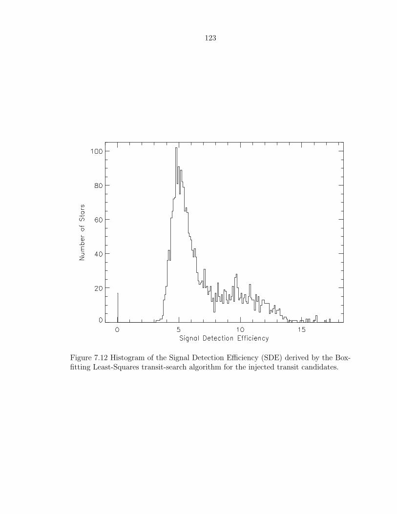
123

Figure 7.12 Histogram of the Signal Detection Efficiency (SDE) derived by the Box-fitting Least-Squares transit-search algorithm for the injected transit candidates.

124

Figure 7.13 Same as figure 7.11, but for the ratio of the transit depth (∆) to the rms(σ) of the TrES photometry. Of the candidates with ∆ ∼> σ, 77% were recovered bythe transit-search algorithm (marked in green; the candidates not recovered are inred).

125

r-band magnitude has been converted to an approximate Tycho-2 (Høg et al., 2000b)

VT magnitude using the field stars with known VT . Again, the BLS algorithm recovers

the majority (62%) of transit candidates with VT ∼< 13.5 mag, except for the brighter,

saturated stars. These results can be better understood by comparing the transit

depth to the rms (σ) of the photometry for the host star, as shown in figure 7.13.

Of the transit candidates with ∆ ∼> σ, 77% are recovered, with a slight bias against

longer periods.

This suggests that VT ∼< 13.5 mag and ∆ ∼> σ are the limits for the BLS algorithm

as applied to TrES data. Of the 1,459 candidates not recovered by the BLS algorithm,

1,197 had SDE < 6, 868 had VT > 13.5 mag, and 1,230 had ∆ < σ. When these

factors are taken into account, only 39 (1%) candidate transit signals that we would

expected the algorithm to detect were not recovered.

The variation of the recovery rate with stellar magnitude for different orbital

periods, planetary radii, stellar radii and impact parameters is shown in Figures 7.14

and 7.15. As would be expected, the recovery rates drop for the fainter stars (VT >13.5

mag) and the brightest, saturated stars (VT <10.0 mag). The rate also increases for

shorter periods, larger planets, and smaller stars, although the trend is not robust

due to the relatively small number of candidate transits. This bias is not surprising,

as a larger planet and smaller star increases ∆, and a shorter period increases the

number of observed transits. However, the rate does seem to increase slightly with

larger impact parameters, which is surprising. A large impact parameter implies a

V-shaped light curve indicative of an eclipsing binary, rather than the typical transit

light curve. Overall, the recovery rate for the BLS algorithm is about 80% for the

average magnitudes of 11 ≤ VT ≤ 12 mag.

Of the 2,612 injected transit candidates, I recovered 641 visually, compared to

1,153 recovered by the BLS algorithm. I have reproduced the earlier plots showing

the SDEs, magnitudes, and depth-to-rms ratios of the fake candidates in Figures 7.16,

7.17, and 7.18. I have then outlined candidates that I visually recovered with a black

diamond, and those candidates that I visually recovered, but dismissed for some reason

(such as poor phase coverage at transit, or a large depth more typical of an eclipsing

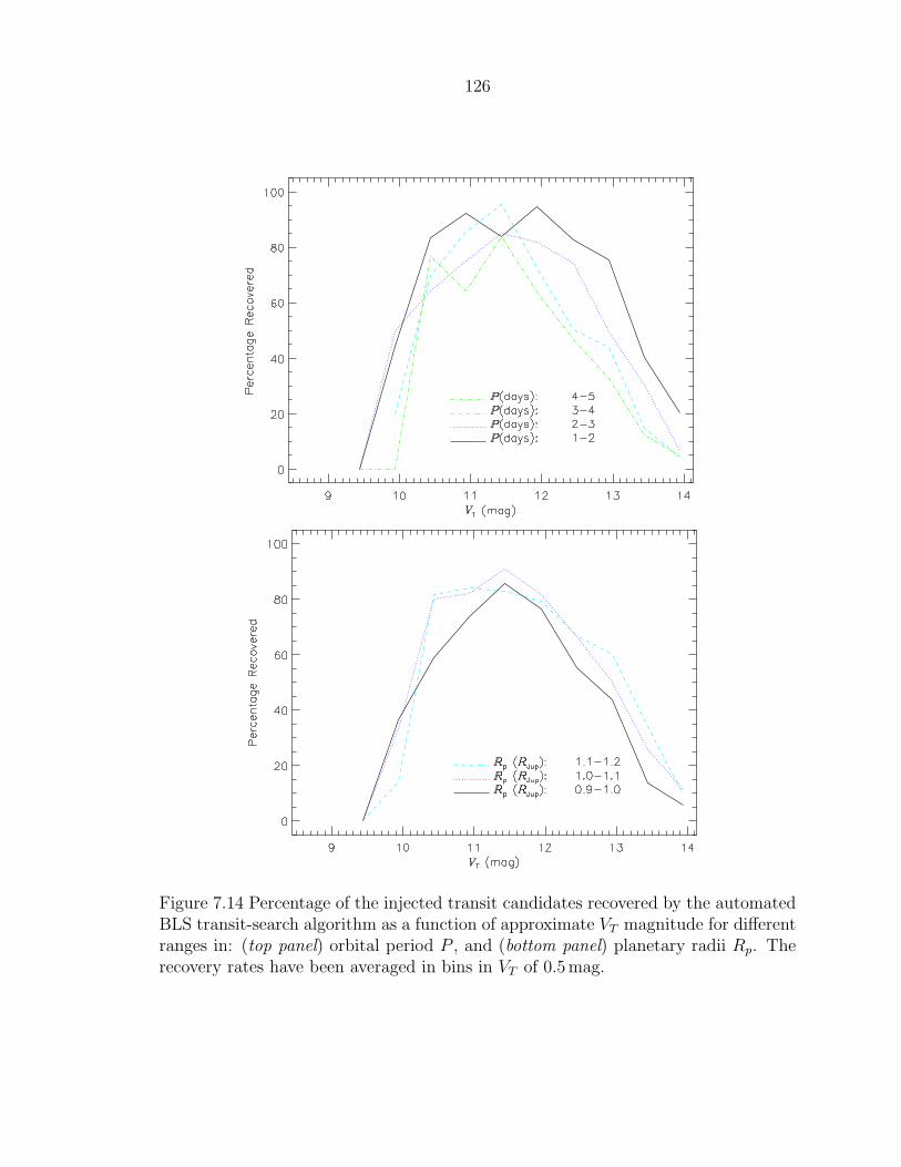
126

Figure 7.14 Percentage of the injected transit candidates recovered by the automatedBLS transit-search algorithm as a function of approximate VT magnitude for differentranges in: (top panel) orbital period P , and (bottom panel) planetary radii Rp. Therecovery rates have been averaged in bins in VT of 0.5 mag.

127

Figure 7.15 Same as for figure 7.14, but for: (top panel) stellar radii R⋆, and (bottompanel) impact parameters b.

128

Figure 7.16 (Top) As for top panel of figure 7.11, except that here the candidatesoutlined in black were visually recovered, and those outlined in blue were visuallyidentified but discarded. (Bottom) Same as the top panel, but for approximate VT

magnitudes versus orbital period for the injected transit candidates.

129

Figure 7.17 Histogram of the Signal Detection Efficiency (SDE) derived by the Box-fitting Least-Squares transit-search algorithm for the injected transit candidates thatwere visually recovered.

130

Figure 7.18 Same as figure 7.16, but for the ratio of the transit depth (∆) to the rms(σ) of the TrES photometry plotted versus the orbital period for the injected transitcandidates.

131

binary), with a blue diamond. We can see that although I visually recovered many

of the candidates, there are several candidates with large SDEs, bright magnitudes

and high depth-to-rms ratios that I missed. I also discarded several candidates with

large SDEs. We can also see that I recovered some of the candidates that failed

my recovery test for the BLS algorithm, although I dismissed them as spurious.

I examined the properties of the BLS-recovered candidate transits that I did not

visually identify or that I dismissed. I found that 71% were faint (VT > 13.5 mag),

and 52% had a depth less than the scatter of the photometry. This would indicate that

I could not visually distinguish these signals from spurious detections in poor-quality

photometry, despite the fact that these signals were recovered by the BLS algorithm.

About 20% had periods or depths outside the limits of my transit plotting code, and

hence were skipped and never viewed. Although these limits were imposed to reduce

the number of false detections due to bad data from a single night of observation,

the resulting high fraction of missed transit signals suggests revisiting this step of my

transit search. Finally, 25% of the candidates that I would not have pursued had

depths greater than 0.03 mag. figure 7.5 shows how relatively few transits with such

large depths would be expected in a field survey such as ours. Our early experience

with pursuing such candidates has reinforced their poor return, and we normally do

not consider them a worthwhile investment. Having accounted for all but 12% (82)

of the transit candidates that I did not visually recover, I examined the light curves

of the remaining candidates with an SDE ≥ 8. I confirmed that for all but a few I

rejected the transit light curve as having few data points within the transit.

The variation of the recovery rate with stellar magnitude for different orbital per-

iods, planetary radii, stellar radii and impact parameters is shown in Figures 7.19

and 7.20. These plots show roughly the same trend in magnitudes, periods, impact

parameters and object sizes as displayed by the BLS algorithm recovery rates. How-

ever, the maximum recovery rates is reduced by ∼20% in each case.

132

Figure 7.19 Percentage of the injected transit candidates visually recovered as a func-tion of approximate VT magnitude for different ranges in: (top panel) orbital periodP , and (bottom panel) planetary radii Rp. The recovery rates have been averaged inbins in VT of 0.5 mag.

133

Figure 7.20 Percentage of the injected transit candidates visually recovered as a func-tion of approximate VT magnitude for different ranges in: (top panel) stellar radii R⋆,and (bottom panel) impact parameters b. The recovery rates have been averaged inbins in VT of 0.5 mag.

134

7.5 Discussion

I have shown that the ability of the BLS transit-search algorithm to recover a candi-

date transit signal has the expected dependence on the brightness of the target star

and the scatter of the photometry. Few of the candidates with optimal brightness and

low scatter were not recovered by the algorithm. I have also tested my own ability

to visually identify a strong transit signal in my data. I clearly do not identify every

candidate correctly recovered by the BLS algorithm, but this is mainly the case for

the faintest stars in our field. However, even for the average-magnitude stars (such

as the host star of TrES-2 with V = 11.4 mag) I have missed some candidates, and

this begs further investigation. In the end, one must accept the loss of some real

detections to avoid being overwhelmed by the data. I find the recovery rate of my

visual analysis to be 87% for those transit candidates that had a sufficiently high

signal-to-noise ratio.

I have found a mild dependence in my transit recovery rates on planetary and

stellar radii and on orbital period. This is in contrast to the similar analysis performed

by Gilliland et al. (2000), who found a strong bias with the planet radius.

135

Chapter 8

Summary

I have presented the results of my thesis work as part of the Trans-atlantic Exoplanet

Survey (TrES) for transiting exoplanets. Using a ten-centimeter telescope to monitor

19 fields each containing 6,000–36,000 stars, I have identified 67 candidate transiting

systems. To date, three of these have been confirmed by determining the spectroscopic

orbit of the host star caused by the planetary companion. Due to the small number of

known transiting exoplanets, this is a noticeable contribution to the field, especially

since these transiting systems are bright enough to be within the reach of HST,

Spitzer, and future JWST observations.

I rejected the majority of the candidates as astrophysical false positives. (The

status of the remaining candidates is not yet fully determined.) This rejection was

made on the basis of my follow-up photometric observations as well as spectroscopy

and photometry obtained by the TrES team. The experience of the TrES team with

efficiently identifying these impostors has resulted in a high yield from the resource-

intensive high signal-to-noise ratio, high-precision spectroscopy that I have obtained

with Keck/HIRES.

The TrES team have also encountered several blended eclipsing binaries that were

quite difficult to identify correctly. However, as a result of a detailed examination

of one-meter class photometry and spectroscopy, we removed these from our list

without the need of larger telescopes. One of these blended systems that I identified

from Sleuth data did not show any spectroscopic evidence of the eclipsing binary, but

was later shown to have a color-dependent eclipse depth, indicative of its true nature.

136

I have conducted followup of the planets that I detected. My analysis of the Spitzer

observations of TrES-2 concluded that this planet has indeed the expected circular

orbit of a hot Jupiter, and that the spectrum shows no clue of the atmospheric

composition, although the scheduled additional observations of the planet are critical

to confirm this.

Looking toward the future, I will be continuing to observe with Sleuth as part of

TrES. Based on the yield of transiting planets from my thesis work, I expect to detect

perhaps as many as three additional planets during the remainder of the survey. I

will obtain additional Spitzer observations of TrES-2 (and hopefully the new TrES

planets) during the remaining lifetime of the instrument, and continue to probe the

exoplanetary atmospheres. I will also be completing my analysis of the survey yield,

from which I will determine the effect of the human determinant on the recovery of

candidate transiting systems.

137

Appendix A

TrES-4: A Transiting Hot Jupiterof Very-Low Density1

Abstract

We report the discovery of TrES-4, a hot Jupiter that transits the star GSC 02620-

00648 every 3.55 days. From high-resolution spectroscopy of the star we estimate a

stellar effective temperature of Teff = 6100 ± 150 K, and from high-precision z and

B photometry of the transit we constrain the ratio of the semi-major axis a and

the stellar radius R⋆ to be a/R⋆ = 6.03 ± 0.13. We compare these values to model

stellar isochrones to constrain the stellar mass to be M⋆ = 1.22 ± 0.17M⊙. Based

on this estimate and the photometric time series, we constrain the stellar radius to

be R⋆ = 1.738 ± 0.092R⊙ and the planet radius to be Rp = 1.674 ± 0.094RJup. We

model our radial-velocity data assuming a circular orbit and find a planetary mass

of 0.84 ± 0.10MJup. Our radial-velocity observations rule out line-bisector variations

that would indicate a specious detection resulting from a blend of an eclipsing binary

system. TrES-4 has the largest radius and lowest density of any of the known transit-

ing planets. It presents a challenge to current models of the physical structure of hot

Jupiters, and indicates that the diversity of physical properties among the members

of this class of exoplanets has yet to be fully explored.

1This chapter has been accepted by the Astrophysical Journal Letters as Mandushev, O’Donovan,et al. 2007.

138

A.1 Understanding the Mass–Radius Relations of

Exoplanets

Despite the ever increasing number of discovered transiting planets (19 at the time of

writing), our understanding of the relationships between host star properties and the

planets’ physical and orbital parameters is still incomplete. While the mass-radius

relation for most transiting planets agrees with the models (Charbonneau et al.,

2007a), several planets have either too high or too low densities. In particular,

HD209458b (Knutson et al., 2007b), HAT-P-1b (Bakos et al., 2007), and WASP-1b

(Collier Cameron et al., 2007) all have much larger radii and lower densities than ex-

pected for planets of their mass and distance from the host star. Several mechanisms

for explaining this discrepancy have been proposed, among them different internal

heat sources (Guillot & Showman, 2002, Bodenheimer, Laughlin, & Lin, 2003), in-

creased planetary atmospheric opacities (Burrows et al., 2007), and less efficient heat

transport as a result of interior composition gradient (Chabrier & Baraffe, 2007). Our

Trans-atlantic Exoplanet Survey (TrES) has previously announced the discovery of

three transiting planets (Alonso et al., 2004a; O’Donovan et al., 2006a, see chapter 4;

O’Donovan et al., 2007b, see chapter 5), each with distinctive properties. We de-

scribe here the newly discovered transiting planet TrES-4, whose mean density of

ρ = 0.222 ± 0.045 g cm−3 is the lowest of all known exoplanets with measured radii

and masses.

A.2 Photometry and Spectroscopy of TrES-4

We monitored a 5.◦8 × 5.◦8 field in Hercules with the Lowell Observatory Planet

Search Survey Telescope (PSST, Dunham et al., 2004) and the Sleuth telescope

(O’Donovan et al., 2004) at Palomar Observatory between UT 2006 May 6 and 2006

August 2. All images were processed and the photometry and transit search carried

out as described in Dunham et al. (2004). Both telescopes detected transits of the

host star GSC 02620-00648: PSST observed 2 full and 1 partial transits, and Sleuth

139

observed 3 full and 4 partial transits. The shape of the events were consistent with

the transit of a Jupiter-sized planet across an F dwarf, and we undertook a program

of follow-up observations to confirm the planetary nature of the object.

We observed the candidate with the CfA Digital Speedometer (Latham, 1992)

from 2006 September to 2007 April. We obtained 7 spectra covering 45 A centered

at 5187 A, with a resolving power of λ/∆λ ≈ 35,000 and S/N between 11 and 13 per

resolution element. This spectral region includes the gravity-sensitive Mg b triplet

and the host star properties derived from an analysis of this region will depend on

the star’s metallicity. We obtained the radial velocities (RVs) by cross-correlation

against a synthetic template chosen from a large library of calculated spectra based

on Kurucz model atmospheres (see Nordstroem et al., 1994; Latham et al., 2002).

These velocities have a typical precision of 0.5 km s−1and they show no significant

variation within the errors . We derived the effective temperature (Teff) and projected

rotational velocity (v sin i) by comparing our observed spectra against synthetic spec-

tra with a wide range of parameters (see Torres, Neuhauser, & Guenther 2002). The

values of Teff) and v sin i are listed in Table A.1, and assume [Fe/H] = 0.0. We

also estimate the surface gravity to be log g = 3.8 ± 0.2. We combined the Johnson-

Cousins photometry that we obtained (see below) with archive 2MASS data, and

used the color-temperature calibrations for dwarfs by Ramırez & Melendez (2005)

and Casagrande, Portinari, & Flynn (2006) to estimate Teff . The average result,

Teff = 6130 ± 80 K, is consistent with the spectroscopic value.

The mass and radius of the star were determined on the basis of the spectroscopic

Teff , the value of a/R⋆ derived from the light curve fit described below, and an assumed

metallicity of [Fe/H] = 0.0 ± 0.2. The quantity a/R⋆ is closely related to the stellar

density, and is determined in this case with much higher relative precision than log g.

It is therefore a better proxy for luminosity (see Sozzetti et al., 2007). Following those

authors, we searched for the best match between stellar evolution models interpolated

to a fine grid in age and metallicity and the three observables, within the stated errors.

Uncertainties were derived from the full range in M⋆ and R⋆ allowed by the isochrones

within observational errors. A comparison with stellar evolution models from the

140

Table A.1. TrES-4 host star

Parameter Units Value Source

RA J2000.0 17h53m13.s05 1Decl. J2000.0 +37◦12′42.′′6 1GSC 02620-00648[µα, µδ] mas yr−1 [−6.5,−23.5] 1V 11.592 ± 0.004 2B − V 0.520 ± 0.007 2V − RC 0.312 ± 0.008 2V − IC 0.601 ± 0.008 2J 10.583 ± 0.018 3J − H 0.233 ± 0.024 3J − Ks 0.253 ± 0.026 3M⋆ M⊙ 1.22 ± 0.17 2R⋆

a R⊙ 1.738 ± 0.092 2L⋆ L⊙ 3.74 ± 0.86 2Teff K 6100 ± 150 2log g 4.045 ± 0.044 2v sin i km s−1 9.5 ± 1.0 2Age Gyr 4.7 ± 2.0 2Distance pc 440 ± 60 2

. .

aThis value of R⋆ is derived from fitting the entirelight curve and is better constrained than the valueobtained solely from the stellar evolution models(section A.2). The uncertainty in R⋆ includes boththe statistical uncertainty of 0.044 R⊙ and the 14%uncertainty in M⋆

References. — (1) UCAC2 (Zacharias et al.,2004); (2) this paper; (3) 2MASS (Skrutskie et al.,2006)

141

Table A.2. TrES-4 planet parameters

Parameter Units Value

P days 3.553945 ± 0.000075Tc HJD 2 454 230.9053 ± 0.0005a AU 0.0488 ± 0.0022i deg 82.81 ± 0.33a/R⋆ 6.026 ± 0.131b = a cos i/R⋆ 0.755 ± 0.015K m s−1 97.4 ± 7.2γ m s−1 +23.7 ± 5.8Mp MJup 0.84 ± 0.10Rp

a RJup 1.674 ± 0.094ρ g cm−3 0.222 ± 0.045log g 2.871 ± 0.038 ±Rp/R⋆ 0.09903 ± 0.00088

.

aThe uncertainty in Rp includes both the statisticaluncertainty of 0.053 RJup and the 14% uncertainty inM⋆ from table A.1

series by Yi et al. (2001) yielded M⋆ = 1.22 ± 0.17 M⊙, R⋆ = 1.738 ± 0.092 R⊙, and

log g = 4.045 ± 0.034. This value of log g is consistent with, but better constrained

than the spectroscopic estimate. The age we derive is 4.7±2.0 Gyr, and the predicted

absolute visual magnitude (MV = 3.36 ± 0.27 mag) implies a distance of 440 ± 60 pc,

ignoring extinction. The error estimates above do not include possible systematic

errors in the stellar evolution models. The gravity, radius and age estimates for the

host star indicate that this is an evolved star at the base of the subgiant branch.

In order to characterize the host star, we obtained off-transit BV (RI)C photom-

etry of TrES-4 on UT 2007 April 14 with the 1.05-meter Hall telescope at Lowell

Observatory in combination with an 2048×2048 pixels SITe CCD. We calibrated the

photometry using 7 standard fields from Landolt (1992). The results are listed in

table A.1 together with other relevant data for the host star of TrES-4.

We carried out high-precision in-transit z-band photometry of TrES-4 on UT 2007

142

Figure A.1 High-precision follow-up z-band and B-band photometry of TrES-4. Theplot shows the relative flux (including the color-dependent extinction correction) ofthe TrES-4 system as a function of time relative to the center of transit, adopting theephemeris in Table A.2. Each light curve is labeled with the telescope and date ofobservation. The residuals from the simultaneous fits (solid lines) are shown beloweach light curve.

143

Table A.3. Radial-velocity measurements of TrES-4

HJD RV (m s−1)

2454187.07793 97.5 ± 11.82454188.11122 58.9 ± 9.42454189.02631 −76.5 ± 11.62454189.14920 −73.9 ± 10.3

May 3 and UT 2007 May 10 with KeplerCam (see, e.g., Holman et al., 2006) at the

Fred L. Whipple Observatory (FLWO) 1.2-meter telescope, and B-band photometry

on UT 2007 May 10 using NASACam at the Lowell Observatory 0.8-meter telescope.

With KeplerCam we gathered 373 and 540 z-band 30-second exposures on UT 2007

May 3 and UT 2007 May 10, respectively. With NASACam, we obtained 192 60-

second B-band exposures. For both data sets, we derived differential fluxes relative

to an ensemble of local comparison stars. The photometry is shown in figure A.1.

We obtained high-precision RV measurements of TrES-4 on UT 2007 March 27–

29, using HIRES and its I2 absorption cell (Vogt et al., 1994) on the Keck I telescope.

Our spectra have a nominal resolving power λ/∆λ ≃ 55 000 and a typical signal-

to-noise ratio S/N ∼ 120 pixel−1. We used nine echelle orders in the wavelength

range 3200–8800 A to derive the velocities for TrES-4. The four star-plus-I2 spectra

(plus one I2-free template exposure) provide good coverage of the critical phases.

As the ephemeris of the system is fixed, RV data are needed only to determine the

amplitude and systemic velocity of the orbit. In these cases (see Konacki et al., 2003)

a few measurements are enough. We extracted and reduced all raw spectra using the

MAKEE software written by T. Barlow (Sozzetti et al., 2006a). The final RV values

are listed in table A.3. The typical precision of the radial velocities 〈σRV 〉 ≃ 10 m s−1

is slightly degraded by the modest stellar rotation. The high-resolution, high S/N

Keck spectra were then used to rule out blend scenarios (see below), and they are

presently being analyzed for improved characterization of the host star.

We fit a Keplerian orbit to these data assuming zero eccentricity as a good first ap-

144

Figure A.2 (Top) Radial velocity observations of TrES-4 obtained with Keck/HIRESusing the I2 cell, shown relative to the center of mass and adopting the ephemeris intable A.2. The best-fit orbit (solid line) is overplotted. (Middle) Residuals from thebest-fit model to the radial velocities. (Bottom) Bisector spans shifted to a medianof zero, for each of the iodine exposures as well as for the template (which is shownas an additional point at phase 0.669).

145

proximation, as expected from theoretical arguments for a period as short as 3.55 days.

The period and epoch of transit were held fixed. The rms of this fit is 11 m s−1, which

is similar to the internal errors of the velocities. The parameters of this orbital solution

are listed in table A.2. We find Mp sin i = 0.731 ± 0.057 [(M⋆ + Mp)/M⊙]2/3 MJup.

The orbit is displayed in figure A.2 (top panel) along with the observations, and

residuals are shown in the middle panel.

We investigated the possibility that the RV variations we measured are the result

of distortions in the line profiles caused by contamination from an unresolved eclipsing

binary (Santos et al., 2002; Torres et al., 2005), instead of being caused by a planetary

companion. We cross-correlated each Keck spectrum against a synthetic template

matching the properties of the star, and averaged the correlation functions over all

orders blueward of the region affected by the I2 lines. From this representation of

the average spectral line profile we computed the mean bisectors, and as a measure

of the line asymmetry we calculated the “bisector spans” as the velocity difference

between points selected near the top and bottom of the mean bisectors (Torres et al.,

2005). If the RV variations were the result of a blend with an eclipsing binary, we

would expect the line bisectors to vary in phase with the photometric period with

an amplitude similar to that of the velocities (Queloz et al., 2001; Mandushev et al.,

2005). Instead, we detect no variation in excess of the measurement uncertainties

(see figure A.2, bottom panel), and we conclude that the RV variations are real and

that the star is orbited by a Jovian planet.

A.3 Properties of TrES-4 and Discussion

We analyzed the two z-band and one B-band photometric time series using the an-

alytic light curves of Mandel & Agol (2002). We assumed a circular orbit and a

quadratic stellar limb-darkening law, fixing the coefficients at the color-dependent

values tabulated in Claret (2000, 2004) for the spectroscopically estimated Teff and

log g, and assuming solar metallicity. We first estimated the time of center of transit

Tc by fitting a model light curve to the z data gathered on UT 2007 May 10. We then

146

determined the orbital period P by combining these data with the TrES discovery

data (which affords a baseline of 1.0 yrs)varying the trial values of P . We then fixed

the values of Tc and P (stated in table A.2) in the subsequent analysis.

Our model has six free parameters: the planet radius Rp, the stellar radius R⋆,

the orbital inclination i, and the color-dependent extinction for each of the three pho-

tometric datasets, kz1, kz2, and kB. We assume that the observed flux is proportional

to e−km, where m denotes the air mass. The values of Rp and R⋆ as constrained by

the light curves alone are covariant with M⋆. In our analysis, we first estimated the

quantity a/R⋆ which is independent of the assumed value of M⋆, and then used this

estimate to constrain the value of M⋆ from stellar isochrones (Sozzetti et al., 2007;

Holman et al., 2007b). We then fixed M⋆ = 1.22 M⊙, and estimated the system-

atic error in the radii using the scaling relations Rp ∝ R⋆ ∝ M1/3⋆ (see footnote to

table A.1).

We found first the values of Rp, R⋆, i, kz1, kz2, and kB that minimized the χ2 using

the AMOEBA algorithm (Press et al., 1992). This model is shown as the solid curves

in figure A.1. We then conducted a Markov Chain Monte Carlo analysis similar to

that described in Holman et al. (2006), Charbonneau et al. (2007b), and Winn et al.

(2007). We created two MCMC chains with 400,000 points each, one starting from the

best-fit values and one starting from a random perturbation to those values. We then

rejected the first 23% of the points to minimize the impact of the initial conditions

and found the results from the two chains to be indistinguishable. We examined the

histograms of the six parameters, as well as the histograms for several combinations of

parameters relevant to anticipated follow-up studies. We assigned the optimal value

to the median, and the 1-σ errors to the symmetric range about the median than

encompassed 68.3% of the values. We list these estimates in table A.2.

TrES-4 has the largest radius and the lowest density of all exoplanets whose mass

and radius are known, and as such presents new challenges for the theory of ir-

radiated gas giants. Burrows et al. (2007) suggested that increased planetary at-

mospheric opacities and the inclusion of a transit radius correction (Baraffe et al.,

2003; Burrows, Sudarsky, & Hubbard, 2003) can explain the radii of all large plan-

147

ets. It appears, however, that TrES-4’s radius is still too large for its mass, age

and insolation. In terms of mass and distance to the host star TrES-4 is similar to

HD 209458, but has nearly 30% larger radius (Rp = 1.67 RJup versus Rp = 1.32 RJup).

Because of the higher host star luminosity TrES-4 receives about twice the stellar

flux, but it is unlikely that the radius difference can be explained solely by the higher

stellar irradiation. For example, HAT-P-1b, which has about the same radius as

HD 209458 and is the only other planet with ρ < 0.3 g cm−3, receives only 60%

of the flux that HD 209458 does. None of the recent models of hot Jupiters (e.g.,

Fortney, Marley, & Barnes, 2007; Burrows et al., 2007) can predict a radius as large

as that of TrES-4 at its orbital separation for the estimated age and for any mass,

even when higher atmospheric opacities are considered and allowance for the transit

radius correction is made.

The properties of TrES-4 and its host star allow for many interesting follow-up

studies, some of which are already underway. The large radius of TrES-4 in the visual

suggests that it may have an extended outer atmosphere, similar to that detected

around HD 209458 in Lyman α by Vidal-Madjar et al. (2003). If such an extended

envelope is caused by mass loss through the planet’s Roche lobe boundary, TrES-4

may have an even bigger envelope because of its smaller Roche limit: RRoche ≈ 3.5 Rp

versus RRoche ≈ 4.4 Rp for HD209458b (Erkaev et al., 2007). Moreover, TrES-4 might

be in a strong hydrodynamic “blow-off” regime where the outer atmospheric layers

are detached from the planet’s gravitational field and escape in a comet-like tail

(Vidal-Madjar et al., 2003; Lecavelier des Etangs et al., 2004).

The relatively fast rotation (v sin i = 9.5 km s−1) and brightness of the TrES-4’s

host star, as well as the planet’s size, are favorable for measuring the Rossiter-

McLaughlin effect (RME; see, e.g., Gaudi & Winn, 2007). Of particular interest

is the angle between the star’s spin axis and the planet’s orbital plane, as it can

provide information about the possible mechanisms of the planet migration and in-

teraction with the disk. The semi-amplitude of the RME is proportional to v sin i and

to (Rp/R⋆)2 and we estimate that for TrES-4 the RME can reach about 90 m s−1, or

roughly equal to the semi-amplitude of its orbital velocity.

148

Appendix B

Properties of Known Transiting Systems

As a reference to the interested reader, I include here tables B.1 and B.2, which

list various properties of the currently known transiting planets and their host stars.

Certain trends in these properties are referred to in chapter 1, and the tables will also

help put into context statements made in other chapters.

149

Table B.1. Properties of the known transiting planets

Planet mp rp a P K b e(MJup) (RJup) (AU) (days) (m s−1)

HD 209458b 0.69 1.31 0.045 3.525 86 0.47 0.07OGLE-TR-56b 1.45 1.23 0.022 1.212 167 0.85 · · ·OGLE-TR-113b 1.35 1.08 0.023 1.432 229 0.07 · · ·OGLE-TR-132b 1.19 1.13 0.031 1.689 141 0.41 · · ·OGLE-TR-111b 0.52 1.07 0.047 4.016 78 0.40 · · ·TrES-1 0.75 1.08 0.039 3.030 115 0.28 0.00OGLE-TR-10b 0.57 1.06 0.401 3.101 80 0.78 · · ·HD 149026 0.33 0.73 0.042 2.876 43 0.51 · · ·HD 189733 1.15 1.26 0.031 2.219 205 0.65 · · ·XO-1b 0.90 1.18 0.049 3.941 116 0.14 · · ·TrES-2 1.28 1.24 0.037 2.471 181 0.84 0.00HAT-P-1b 0.53 1.20 0.055 4.465 60 0.70 · · ·WASP-1b 0.89 1.44 0.038 2.519 115 0.70 · · ·WASP-2b 0.88 1.04 0.031 2.152 155 0.44 · · ·TrES-3 1.92 1.30 0.023 1.306 378 0.83 · · ·HAT-P-2b 8.17 1.18 0.069 5.633 884 0.00 0.51XO-2b 0.57 0.97 0.037 2.616 85 0.20 · · ·GJ 436b 0.07 0.35 0.029 2.644 18 0.84 0.16TrES-4 0.87 1.70 0.050 3.554 97 0.76 · · ·HAT-P-3b 0.60 0.89 0.039 2.900 89 0.51 · · ·

150

Table B.2. Properties of the known transiting-planet host stars

Star M⋆ R⋆ Magnitude d Teff log (g) [Fe/H](M⊙) (R⊙) (mag) (pc) (K) (dex) (dex)

HD 209458 1.10 1.20 V = 7.65 47 5942 4.25 +0.04OGLE-TR-56 1.04 1.10 V = 16.60 1500 6119 4.21 +0.25OGLE-TR-113 0.78 0.77 I = 14.42 1500 4804 4.52 +0.15OGLE-TR-132 1.34 1.41 I = 15.72 1500 6411 4.86 +0.43OGLE-TR-111 0.81 0.83 I = 15.55 1500 5044 4.51 +0.19TrES-1 0.89 0.83 V = 11.79 157 5226 4.40 +0.06OGLE-TR-10 1.00 1.10 I = 14.93 1500 6075 4.54 +0.28HD 149026 1.30 1.45 V = 8.15 79 5888 4.26 +0.36HD 189733 0.82 0.76 V = 7.67 19 4954 4.53 −0.03XO-1 1.00 0.93 V = 11.85 200 5750 4.38 +0.02TrES-2 1.08 1.00 V = 11.41 230 5960 4.40 −0.15HAT-P-1 1.12 1.12 V = 10.40 139 5975 4.45 +0.13WASP-1 1.15 1.24 V = 11.79 · · · 6200 4.30 · · ·WASP-2 0.79 0.78 V = 11.98 · · · 5200 4.30 · · ·TrES-3 0.90 0.80 V = 12.40 450 5720 4.60 · · ·HAT-P-2 1.35 1.80 V = 8.71 135 6290 4.22 +0.12XO-2 0.98 0.96 V = 11.18 149 5340 4.45 +0.45GJ 436 0.44 0.44 V = 10.68 10 3350 4.50 −0.32TrES-4 1.77 1.28 V = 11.59 450 6100 4.06 · · ·HAT-P-3 0.94 0.82 V = 11.56 140 5185 4.61 +0.27

151

Appendix C

The Box-fitting Least-Squares (BLS)Transit-Search Algorithm

As a reference to the reader, in this appendix I summarize the method to search for

periodic transits signals in photometric data proposed by Kovacs, Zucker, & Mazeh

(2002). For easy comparison with the reference paper, in general I use the authors’

notation.

C.1 A General Description of the BLS Algorithm

When a dark planet transits the disk of a star, the resulting U-shaped light curve

(see, e.g., figure 7.7) requires a complex analytical description (Mandel & Agol, 2002).

Trying to fit such a model to each light curve from a transit survey such as the Trans-

atlantic Exoplanet Survey (TrES) would be prohibitively computationally intensive.

Instead, Kovacs et al. (2002) proposed searching for a periodic transit signal (of pe-

riod P0) using a much simpler box fit, that is assuming a light curve with two discrete

levels (H and L), with an ingress phase φ, and with a short fractional duration (q) at

the lower level, L. The value of q is assumed to lie within [0.01, 0.10], as expected for

almost all transiting planets (Defay, Deleuil, & Barge, 2001). For TrES time series

of differential magnitudes, we also assume H = 0, and hence L = δ, the depth of the

transit. For example of a light curve of a (fake) transit candidate, with the box-fit

light curve overplotted, see figure 7.10.

The BLS algorithm takes as input a photometric time series, a range of periods

152

[P1, . . . , Pnp] to search, and the number of trial periods (np) and bins (nb) to use. The

period step separating each trial period is then ∆p = (Pnp−P1)/np. For a given trial

period Pi, the time series is folded and averaged in the nb bins. The algorithm then

computes the Signal Residue (a measure of the quality of the fit; see below), and the

best-fit qi, δi, and φi for this trial period.

The best-fit period P is the trial period that gives the largest Signal Residue. The

overall best-fit parameters from the BLS algorithm for the input time series are then

P , and the corresponding {q, δ, φ}.

C.2 The Signal Residue and Signal Detection

Efficiency

Assume we have a time series phased using a trial period Pi. Let us denote the folded

time series by {xi}, i = 1, 2, . . . , n. Each data point xi has an associated uncertainty

σi, and a corresponding weight

wi =

(

σ2i

n∑

j=1

1

σ2j

)

−1

.

Now suppose that in-transit occurs in the bins (i1, i2), under the condition that q =

(i2 − i1)/nb lies within the above range. Define

r(i1, i2) =

i2∑

i=i1

wi,

that is, the sum of the weights of the in-transit data, and

s(i1, i2) =

i2∑

i=i1

wixi,

153

i.e., the weighted sum of the in-transit data. The Signal Residue (SR) of the time

series for Pi is then defined as

SR = MAX

{

[

s2(i1, i2)

r(i1, i2)[1 − r(i1, i2)]

]1

2

}

.

The least-squares best-fit for the time series is then computed by finding the period

P that maximizes SR. The largest Signal Residue, SR, has associated in-transit bins

(i1, i2). The best-fit transit depth δ can then be derived using

δ =SR

√

r(i1, i2)[1 − r(i1, i2)].

The best-fit ingress phase is i1/nb, and the best-fit fractional transit duration is

q =i2 − i1

nb

.

Once we have derived the best fit for a given time series, we can compute for that

time series the Signal Detection Efficiency (SDE)

SDE = (SR − < SR >)/σ(SR),

where < SR > and σ(SR) are the average and standard deviation, respectively, of

the Signal Residue over the period range tested. The SDE can then be used as a

comparative measure of the strengths of the transit detections in a sequence of time

series, such as the photometry from TrES.

154

Bibliography

Agol, E., Steffen, J., Sari, R., & Clarkson, W. 2005, MNRAS, 359, 567

Alard, C. 2000, A&AS, 144, 363

Alonso, R., et al. 2004a, ApJ, 613, L153

Alonso, R., Deeg, H. J., Brown, T. M., & Belmonte, J. A. 2004b, Astron. Nachr.,

325, 594

Bakos, G., Noyes, R. W., Kovacs, G., Stanek, K. Z., Sasselov, D. D., & Domsa, I.

2004, PASP, 116, 266

Bakos, G. A., Lazar, J., Papp, I., Sari, P., & Green, E. M. 2002, PASP, 114, 974

Bakos, G. A., et al. 2007, ApJ, 656, 552

Baraffe, I., Chabrier, G., Allard, F., & Hauschildt, P. H. 1998, A&A, 337, 403

Baraffe, I., Chabrier, G., Barman, T. S., Allard, F., & Hauschildt, P. H. 2003, A&A,

402, 701

Baraffe, I., Selsis, F., Chabrier, G., Barman, T. S., Allard, F., Hauschildt, P. H., &

Lammer, H. 2004, A&A, 419, L13

Barman, T. 2007, ApJ, 661, L191

Barman, T. S., Hauschildt, P. H., & Allard, F. 2005, ApJ, 632, 1132

Bessell, M. S., & Brett, J. M. 1988, PASP, 100, 1134

Bodenheimer, P., Laughlin, G., & Lin, D. N. C. 2003, ApJ, 592, 555

155

Bodenheimer, P., Lin, D. N. C., & Mardling, R. A. 2001, ApJ, 548, 466

Borucki, W. J., Caldwell, D., Koch, D. G., Webster, L. D., Jenkins, J. M., Ninkov,

Z., & Showen, R. 2001, PASP, 113, 439

Boss, A. P. 1997, Science, 276, 1836

Bouchy, F., Pont, F., Melo, C., Santos, N. C., Mayor, M., Queloz, D., & Udry, S.

2005a, A&A, 431, 1105

Bouchy, F., Pont, F., Santos, N. C., Melo, C., Mayor, M., Queloz, D., & Udry, S.

2004, A&A, 421, L13

Bouchy, F., et al. 2005b, A&A, 444, L15

Bramich, D. M., et al. 2005, MNRAS, 359, 1096

Brown, T. M. 2003, ApJ, 593, L125

Brown, T. M., Charbonneau, D., Gilliland, R. L., Noyes, R. W., & Burrows, A. 2001,

ApJ, 552, 699

Burrows, A., Hubeny, I., Budaj, J., & Hubbard, W. B. 2007, ApJ, 661, 502

Burrows, A., Hubeny, I., & Sudarsky, D. 2005, ApJ, 625, L135

Burrows, A., Sudarsky, D., & Hubbard, W. B. 2003, ApJ, 594, 545

Burrows, A., Sudarsky, D., & Hubeny, I. 2006, ApJ, 650, 1140

Butler, R. P., Marcy, G. W., Williams, E., McCarthy, C., Dosanjh, P., & Vogt, S. S.

1996, PASP, 108, 500

Carpenter, J. M. 2001, AJ, 121, 2851

Casagrande, L., Portinari, L., & Flynn, C. 2006, MNRAS, 373, 13

Chabrier, G., & Baraffe, I. 2007, ApJ, 661, L81

156

Chabrier, G., Baraffe, I., Allard, F., & Hauschildt, P. H. 2005, in ASP Conf. Ser.,

Resolved Stellar Populations, ed. D. Valls-Gabaud & M. Chavez (San Francisco:

ASP) (astro-ph/0509798)

Charbonneau, D., et al. 2005, ApJ, 626, 523

Charbonneau, D., Brown, T. M., Burrows, A., & Laughlin, G. 2007a, in Protostars

and Planets V, ed. B. Reipurth, D. Jewitt, & K. Keil (Tucson: University of Arizona

Press), 701

Charbonneau, D., Brown, T. M., Dunham, E. W., Latham, D. W., Looper, D. L., &

Mandushev, G. 2004, in AIP Conf. Proc. 713, The Search for Other Worlds, ed.

S. S. Holt & D. Deming (New York: AIP), 151

Charbonneau, D., Brown, T. M., Latham, D. W., & Mayor, M. 2000, ApJ, 529, L45

Charbonneau, D., Brown, T. M., Noyes, R. W., & Gilliland, R. L. 2002, ApJ, 568,

377

Charbonneau, D., Noyes, R. W., Korzennik, S. G., Nisenson, P., Jha, S., Vogt, S. S.,

& Kibrick, R. I. 1999, ApJ, 522, L145

Charbonneau, D., Winn, J. N., Everett, M. E., Latham, D. W., Holman, M. J.,

Esquerdo, G. A., & O’Donovan, F. T. 2007b, ApJ, 658, 1322

Charbonneau, D., et al. 2006, ApJ, 636, 445

Christian, D. J., et al. 2006, MNRAS, 372, 1117

Claret, A. 2000, A&A, 363, 1081

Claret, A. 2004, A&A, 428, 1001

Cochran, W. D., Hatzes, A. P., & Paulson, D. B. 2002, AJ, 124, 565

Collier Cameron, A., et al. 2007, MNRAS, 375, 951

157

Cox, A. N. 2000, Allen’s Astrophysical Quantities, 4th Edition (New York: AIP Press

Springer-Verlag)

Creevey, O. L., et al. 2005, ApJ, 625, L127

Cutri, R. M., et al. 2003, 2MASS All Sky Catalog of Point Sources (Amherst: Univ.

Massachusetts Press), http://irsa.ipac.caltech.edu/applications/Gator

Deeg, H. J., & Doyle, L. R. 2001, in Third Workshop on Photometry, ed. W. J. Borucki

& L. E. Lasher, NASA/CP-2000-209614 (Langley Research Center: NASA), 85

Defay, C., Deleuil, M., & Barge, P. 2001, A&A, 365, 330

Delfosse, X., Forveille, T., Segransan, D., Beuzit, J.-L., Udry, S., Perrier, C., &

Mayor, M. 2000, A&A, 364, 217

Deming, D., Brown, T. M., Charbonneau, D., Harrington, J., & Richardson, L. J.

2005a, ApJ, 622, 1149

Deming, D., Harrington, J., Seager, S., & Richardson, L. J. 2006, ApJ, 644, 560

Deming, D., & Seager, S., ed. 2003, ASP Conf. Ser. 294, Scientific Frontiers in Re-

search on Extrasolar Planets (San Francisco: ASP)

Deming, D., Seager, S., Richardson, L. J., & Harrington, J. 2005b, Nature, 434, 740

Drake, A. J. 2003, ApJ, 589, 1020

Dravins, D., Lindegren, L., Mezey, E., & Young, A. T. 1998, PASP, 110, 610

Dunham, E. W., Mandushev, G. I., Taylor, B. W., & Oetiker, B. 2004, PASP, 116,

1072

Erkaev, N. V., Lammer, H., Kulikov, Y. N., Langmayr, D., Selsis, F., Jaritz, G. F.,

& Biernat, H. K. 2007, A&A, submitted (astro-ph/0612729)

Fabrycky, D. C., Johnson, E. T., & Goodman, J. 2007, ApJ, 665, 754

158

Fazio, G. G., et al. 2004, ApJS, 154, 10

Fischer, D. A., & Valenti, J. A. 2003, in ASP Conf. Ser. 294, Scientific Frontiers in

Research on Extrasolar Planets, ed. D. Deming & S. Seager (San Francisco: ASP),

117

Fortney, J. J., Cooper, C. S., Showman, A. P., Marley, M. S., & Freedman, R. S.

2006a, ApJ, 652, 746

Fortney, J. J., Marley, M. S., & Barnes, J. W. 2007, ApJ, 659, 1661

Fortney, J. J., Marley, M. S., Lodders, K., Saumon, D., & Freedman, R. 2005, ApJ,

627, L69

Fortney, J. J., Saumon, D., Marley, M. S., Lodders, K., & Freedman, R. S. 2006b,

ApJ, 642, 495

Fressin, F., Guillot, T., Morello, V., & Pont, F. 2007, A&A, in press (arXiv:0704.1919)

Gaudi, B. S. 2005, ApJ, 628, L73

Gaudi, B. S. 2007, in ASP Conf. Ser. 366, Transiting Extrasolar Planets Workshop,

ed. Afonso, C., Weldrake, D., & Henning, T. (San Francisco: ASP), 273 (astro-

ph/0612141)

Gaudi, B. S., Seager, S., & Mallen-Ornelas, G. 2005, ApJ, 623, 472

Gaudi, B. S., & Winn, J. N. 2007, ApJ, 655, 550

Gilliland, R. L., et al. 2000, ApJ, 545, L47

Girardi, L., Bressan, A., Bertelli, G., & Chiosi, C. 2000, A&AS, 141, 371

Goldreich, P., & Tremaine, S. 1980, ApJ, 241, 425

Gonzalez, G. 1997, MNRAS, 285, 403

Gonzalez, G. 2006, PASP, 118, 1494

159

Gould, A., Dorsher, S., Gaudi, B. S., & Udalski, A. 2006, Acta Astron., 56, 1

Grillmair, C. J., Charbonneau, D., Burrows, A., Armus, L., Stauffer, J., Meadows,

V., Van Cleve, J., & Levine, D. 2007, ApJ, 658, L115

Guillot, T., & Showman, A. P. 2002, A&A, 385, 156

Henry, G. W., Marcy, G. W., Butler, R. P., & Vogt, S. S. 2000, ApJ, 529, L41

Hidas, M. G., et al. 2005, MNRAS, 360, 703

Høg, E., et al. 2000a, A&A, 357, 367

Høg, E., et al. 2000b, A&A, 355, L27

Holman, M. J., & Murray, N. W. 2005, Science, 307, 1288

Holman, M. J., et al. 2007a, ApJ, 655, 1103

Holman, M. J., et al. 2006, ApJ, 652, 1715

Holman, M. J., et al. 2007b, ApJ, 664, 1185

Holt, S. S., & Deming, D., ed. 2004, AIP Conf. Proc. 713, The Search for Other

Worlds (New York: AIP)

Horne, K. 2003, in ASP Conf. Ser. 294, Scientific Frontiers in Research on Extrasolar

Planets, ed. D. Deming & S. Seager (San Francisco: ASP), 361

Hut, P. 1981, A&A, 99, 126

Jenkins, J. M., & Doyle, L. R. 2003, ApJ, 595, 429

Kane, S. R., Collier Cameron, A., Horne, K., James, D., Lister, T. A., Pollacco, D. L.,

Street, R. A., & Tsapras, Y. 2005, MNRAS, 364, 1091

Knutson, H. A., et al. 2007a, Nature, 447, 183

Knutson, H. A., Charbonneau, D., Noyes, R. W., Brown, T. M., & Gilliland, R. L.

2007b, ApJ, 655, 564

160

Konacki, M., Torres, G., Jha, S., & Sasselov, D. D. 2003, Nature, 421, 507

Konacki, M., et al. 2004, ApJ, 609, L37

Korzennik, S. G., Brown, T. M., Fischer, D. A., Nisenson, P., & Noyes, R. W. 2000,

ApJ, 533, L147

Kotredes, L., Charbonneau, D., Looper, D. L., & O’Donovan, F. T. 2004, in AIP

Conf. Proc. 713, The Search for Other Worlds, ed. S. S. Holt & D. Deming (New

York: AIP), 173

Kovacs, G., Bakos, G., & Noyes, R. W. 2005, MNRAS, 356, 557

Kovacs, G., Zucker, S., & Mazeh, T. 2002, A&A, 391, 369

Kurucz, R. 1993, Kurucz CD-ROM 13, ATLAS9 Stellar Atmosphere Programs and

2 km/s Grid (Cambridge: SAO)

Landolt, A. U. 1992, AJ, 104, 340

Lasker, B. M., Sturch, C. R., McLean, B. J., Russell, J. L., Jenkner, H., & Shara,

M. M. 1990, AJ, 99, 2019

Latham, D. W. 1992, in ASP Conf. Ser. 32, Complementary Approaches to Double

and Multiple Star Research, ed. H. A. McAlister & W. I. Hartkopf (San Francisco:

ASP), 110

Latham, D. W. 2003, in ASP Conf. Ser. 294, Scientific Frontiers in Research on

Extrasolar Planets, ed. D. Deming & S. Seager (San Francisco: ASP), 409

Latham, D. W., Stefanik, R. P., Mazeh, T., Mayor, M., & Burki, G. 1989, Nature,

339, 38

Latham, D. W., Stefanik, R. P., Torres, G., Davis, R. J., Mazeh, T., Carney, B. W.,

Laird, J. B., & Morse, J. A. 2002, AJ, 124, 1144

161

Laughlin, G., Wolf, A., Vanmunster, T., Bodenheimer, P., Fischer, D., Marcy, G.,

Butler, P., & Vogt, S. 2005, ApJ, 621, 1072

Lecavelier des Etangs, A., Vidal-Madjar, A., McConnell, J. C., & Hebrard, G. 2004,

A&A, 418, L1

Leggett, S. K. 1992, ApJS, 82, 351

Leigh, C., Collier Cameron, A., Udry, S., Donati, J.-F., Horne, K., James, D., &

Penny, A. 2003, MNRAS, 346, L16

Lin, D. N. C., Bodenheimer, P., & Richardson, D. C. 1996, Nature, 380, 606

Livingston, W., & Wallace, L. 1991, An Atlas of the Solar Spectrum in the Infrared

from 1850 to 9000 cm-1 (1.1 to 5.4 micrometer) (NSO Technical Report 91-001;

Tucson: NSO)

Lovis, C., et al. 2006, Nature, 441, 305

Mandel, K., & Agol, E. 2002, ApJ, 580, L171

Mandushev, G., et al. 2007, ApJL, in press (arXiv:0708.0834), 708

Mandushev, G., et al. 2005, ApJ, 621, 1061

Marcy, G. W., & Butler, R. P. 1992, PASP, 104, 270

Marcy, G. W., Cochran, W. D., & Mayor, M. 2000, in Protostars and Planets IV, ed.

V. Mannings, A. P. Boss, & S. S. Russell (Tucson: University of Arizona Press),

1285

Marley, M. S., Fortney, J., Seager, S., & Barman, T. 2007, in Protostars and Planets

V, ed. B. Reipurth, D. Jewitt, & K. Keil (Tucson: University of Arizona Press),

733

Mayor, M., & Queloz, D. 1995, Nature, 378, 355

Mazeh, T., et al. 2000, ApJ, 532, L55

162

Mazeh, T., Zucker, S., & Pont, F. 2005, MNRAS, 356, 955

McCullough, P. R., Stys, J. E., Valenti, J. A., Fleming, S. W., Janes, K. A., &

Heasley, J. N. 2005, PASP, 117, 783

McCullough, P. R., et al. 2006, ApJ, 648, 1228

McLaughlin, D. B. 1924, ApJ, 60, 22

Miralda-Escude, J. 2002, ApJ, 564, 1019

Monet, D. G., et al. 2003, AJ, 125, 984

Nordstroem, B., Latham, D. W., Morse, J. A., Milone, A. A. E., Kurucz, R. L.,

Andersen, J., & Stefanik, R. P. 1994, A&A, 287, 338

O’Donovan, F. T., et al. 2007a, ApJ, 662, 658

O’Donovan, F. T., et al. 2007b, ApJ, 663, L37

O’Donovan, F. T., Charbonneau, D., & Kotredes, L. 2004, in AIP Conf. Proc. 713,

The Search for Other Worlds, ed. S. S. Holt & D. Deming (New York: AIP), 169

O’Donovan, F. T., et al. 2006a, ApJ, 651, L61

O’Donovan, F. T., et al. 2006b, ApJ, 644, 1237

Park, S. K., & Miller, K. W. 1988, Commun. ACM, 31, 1192

Pepper, J., Gould, A., & Depoy, D. L. 2004, in AIP Conf. Proc. 713, The Search for

Other Worlds, ed. S. S. Holt & D. Deming (New York: AIP), 185

Pollack, J. B. 1984, ARA&A, 22, 389

Pollack, J. B., Hubickyj, O., Bodenheimer, P., Lissauer, J. J., Podolak, M., & Green-

zweig, Y. 1996, Icarus, 124, 62

Pont, F., Bouchy, F., Melo, C., Santos, N. C., Mayor, M., Queloz, D., & Udry, S.

2005, A&A, 438, 1123

163

Pont, F., Zucker, S., & Queloz, D. 2006, MNRAS, 373, 231

Press, W. H., Teukolsky, S. A., Vetterling, W. T., & Flannery, B. P. 1992, Numerical

Recipes in C (Cambridge: Cambridge University Press)

Queloz, D., et al. 2001, A&A, 379, 279

Ramırez, I., & Melendez, J. 2005, ApJ, 626, 465

Rasio, F. A., & Ford, E. B. 1996, Science, 274, 954

Rauer, H., Eisloffel, J., Erikson, A., Guenther, E., Hatzes, A. P., Michaelis, H., &

Voss, H. 2004, PASP, 116, 38

Reipurth, B., Jewitt, D., & Keil, K., ed. 2007, Protostars and Planets V (Tucson:

University of Arizona Press)

Richardson, L. J., Deming, D., Horning, K., Seager, S., & Harrington, J. 2007, Nature,

445, 892

Rossiter, R. A. 1924, ApJ, 60, 15

Rowe, J. F., et al. 2006, ApJ, 646, 1241

Saar, S. H., Butler, R. P., & Marcy, G. W. 1998, ApJ, 498, L153

Sackett, P. D. 1999, in NATO ASIC Proc. 532: Planets Outside the Solar System:

Theory and Observations, ed. J.-M. Mariotti & D. Alloin, 189

Santos, N. C., Israelian, G., & Mayor, M. 2004, A&A, 415, 1153

Santos, N. C., Mayor, M., Naef, D., Pepe, F., Queloz, D., Udry, S., & Blecha, A.

2000, A&A, 361, 265

Santos, N. C., et al. 2002, A&A, 392, 215

Sasselov, D. D. 2003, ApJ, 596, 1327

Sato, B., et al. 2005, ApJ, 633, 465

164

Seager, S., & Mallen-Ornelas, G. 2003, ApJ, 585, 1038

Seager, S., Richardson, L. J., Hansen, B. M. S., Menou, K., Cho, J. Y.-K., & Deming,

D. 2005, ApJ, 632, 1122

Showman, A. P., & Guillot, T. 2002, A&A, 385, 166

Sirko, E., & Paczynski, B. 2003, ApJ, 592, 1217

Skrutskie, M. F., et al. 2006, AJ, 131, 1163

Smith, A. M. S., et al. 2006, MNRAS, 373, 1151

Sozzetti, A., Torres, G., Charbonneau, D., Latham, D. W., Holman, M. J., Winn,

J. N., Laird, J. B., & O’Donovan, F. T. 2007, ApJ, 664, 1190

Sozzetti, A., Torres, G., Latham, D. W., Carney, B. W., Stefanik, R. P., Boss, A. P.,

Laird, J. B., & Korzennik, S. G. 2006a, ApJ, 649, 428

Sozzetti, A., Yong, D., Carney, B. W., Laird, J. B., Latham, D. W., & Torres, G.

2006b, AJ, 131, 2274

Sozzetti, A., et al. 2004, ApJ, 616, L167

Steffen, J. H., & Agol, E. 2005, MNRAS, 364, L96

Stetson, P. B. 1987, PASP, 99, 191

Stetson, P. B. 1992, in ASP Conf. Ser. 25, Astronomical Data Analysis Software and

Systems I, ed. D. M. Worrall, C. Biemesderfer, & J. Barnes, 297

Street, R. A., et al. 2003, in ASP Conf. Ser. 294, Scientific Frontiers in Research on

Extrasolar Planets, ed. D. Deming & S. Seager (San Francisco: ASP), 405

Struve, O. 1952, Observatory, 72, 199

Swain, M. R., Bouwman, J., Akeson, R., Lawler, S., & Beichman, C. 2007, ApJ,

submitted (astro-ph/0702593)

165

Szentgyorgyi, A. H., et al. 2005, BAAS, 37, 1339

Tingley, B. 2003a, A&A, 403, 329

Tingley, B. 2003b, A&A, 408, L5

Tingley, B. 2004, A&A, 425, 1125

Tody, D. 1993, in ASP Conf. Ser. 52, Astronomical Data Analysis Software and

Systems II, ed. R. J. Hanisch, R. J. V. Brissenden, & J. Barnes (San Francisco:

ASP), 173

Torres, G., Konacki, M., Sasselov, D. D., & Jha, S. 2004a, ApJ, 609, 1071

Torres, G., Konacki, M., Sasselov, D. D., & Jha, S. 2004b, ApJ, 614, 979

Torres, G., Konacki, M., Sasselov, D. D., & Jha, S. 2005, ApJ, 619, 558

Torres, G., Neuhauser, R., & Guenther, E. W. 2002, AJ, 123, 1701

Trilling, D. E., Benz, W., Guillot, T., Lunine, J. I., Hubbard, W. B., & Burrows, A.

1998, ApJ, 500, 428

Udalski, A., et al. 2002, Acta Astron., 52, 1

Udalski, A., Pietrzynski, G., Szymanski, M., Kubiak, M., Zebrun, K., Soszynski, I.,

Szewczyk, O., & Wyrzykowski, L. 2003, Acta Astron., 53, 133

Udry, S., et al. 2007, A&A, 469, L43

Udry, S., Fischer, D., & Queloz, D. 2007, in Protostars and Planets V, ed. B. Reipurth,

D. Jewitt, & K. Keil (Tucson: University of Arizona Press), 685

Udry, S., Mayor, M., & Santos, N. C. 2003, A&A, 407, 369

Valenti, J. A., Butler, R. P., & Marcy, G. W. 1995, PASP, 107, 966

Vidal-Madjar, A., et al. 2004, ApJ, 604, L69

166

Vidal-Madjar, A., Lecavelier des Etangs, A., Desert, J.-M., Ballester, G. E., Ferlet,

R., Hebrard, G., & Mayor, M. 2003, Nature, 422, 143

Vogt, S. S., et al. 1994, in Instrumentation in Astronomy VIII, D. L. Crawford & E.

R. Craine eds., Proc. SPIE, 2198, 362

Weldrake, D. T. F., & Sackett, P. D. 2005, ApJ, 620, 1033

Williams, P. K. G., Charbonneau, D., Cooper, C. S., Showman, A. P., & Fortney,

J. J. 2006, ApJ, 649, 1020

Winn, J. N., & Holman, M. J. 2005, ApJ, 628, L159

Winn, J. N., Holman, M. J., & Roussanova, A. 2007, ApJ, 657, 1098

Wolszczan, A., & Frail, D. A. 1992, Nature, 355, 145

Wright, J. T. 2005, PASP, 117, 657

Yi, S., Demarque, P., Kim, Y.-C., Lee, Y.-W., Ree, C. H., Lejeune, T., & Barnes, S.

2001, ApJS, 136, 417

Young, A. T. 1967, AJ, 72, 747

Zacharias, N., Urban, S. E., Zacharias, M. I., Wycoff, G. L., Hall, D. M., Monet,

D. G., & Rafferty, T. J. 2004, AJ, 127, 3043

Zucker, S., & Mazeh, T. 1994, ApJ, 420, 806

Zucker, S., & Mazeh, T. 2002, ApJ, 568, L113