The Determination of Relative Elemental Growth Rate

Plant Physiol. (1 997) 11 3: 1395-1 404

The Determination of Relative Elemental Growth Rate Profiles from Segmenta1 Crowth Rates'

A Methodological Evaluation

Winfried Stefan Petersz* and Nirit Bernstein

lnstitute of Soils and Water, The Volcani Center, P.O. Box 6, Bet Dagan 50250, Israel

~ ~ ~

Relative elemental growth rate (RECR) profiles describe spatial patterns of growth intensity; they are indispensable for causal growth analyses. Published methods of RECR profile determination from marking experiments fall in two classes: the profile i s either described by a series of segmental growth rates, or calculated as the slope of a function describing the displacement velocities of points along the organ. The latter technique is usually considered superior for theoretical reasons, but to our knowledge, no comparative methodological study of the two approaches i s currently available. We formulated a model RECR profile that resembles those reported from primary roots. We established the displacement velocity profile and derived growth trajectories, which enabled us to perform hypothetical marking experiments on the model with varying spac- ing of marks and durations of measurement. RECR profiles were determined from these data by alternative methods, and results were compared to the original profile. We find that with our model plotting of segmental relative growth rates versus segment position provides exact RECR profile estimations, i f the initial segment length i s less than 10% of the length of the whole growing zone, and if less than 20% of the growing zone is displaced past i ts boundary during the measurement. Based on our analysis, we discuss systematic errors that occur in marking experiments.

In developing plants growth is generally not uniform throughout the growing organs, but is confined to distinct zones along which diverse spatial patterns of growth intensity exist (Sachs, 1824b; Esau, 1943; Erickson and Sax, 1956; Silk and Erickson, 1979). Thus, a detailed quantitative description of spatial growth profiles is fundamental for physiological inquiries into the regulation of growth and its alteration under stress conditions. Parameters involved in the control of the growth process might be identified by comparing spatial patterns of growth intensity with spatial patterns of the parameter in question, whether it be con- tents (as with nutritional elements or phytohormones), deposition rates (as with cell wall material), catalytic activ-

This work was supported by grant no. 2360-93 from the Bina- tional Agricultura1 Research Fund (BARD). This is contribution no. 1918-E, 1996 series, from the Agricultural Research Organization, The Volcani Center, Bet-Dagan, Israel.

Present address: Botanisches Institut 1, Senckenbergstrasse 17- 21, D-35390 Giessen, Germany.

* Corresponding author; e-mail [email protected] giessen.de; fax 49-641-993-5119.

ity (as with cell wall-loosening enzymes), or others. Con- sequently, quantitative spatial growth analysis has formed the basis for the study of the regulation of straight elongation growth in leaves (Schnyder and Nelson, 1988; Mac- Adam et al., 1992; Bernstein et al., 1993a, 1995), in shoots (Silk and Abou Haidar, 1986; Paolillo and Rubin, 1991; Saab et al., 1992), and in roots (Goodwin, 1972; Verse1 and Mayor, 1985; Spollen and Sharp, 1991; Pritchard et al., 1993). Tropic (Barlow and Rathfelder, 1985; Berg et al., 1986; Ishikawa et al., 1991) and spontaneous curvature (Silk and Erickson, 1978; Silk, 1989), as well as two-dimensional leaf growth (Richards and Kavanagh, 1943; Erickson, 1966; Wolf et al., 1986) and tip growth (Chen, 1973) have been investigated using the same approach. Obviously, a highly reliable method of spatial growth characterization is crucial for analyses of this type.

To obtain information on spatial growth patterns, bota- nists have performed so-called marking experiments for almost three centuries (Hales, 1727; Ohlert, 1837; Sachs, 1874a; Brumfield, 1942). In such tests, which proved to be particularly fruitful in the case of pure elongation growth, segments along an organ are defined by artificial or ana- tomical markers. Elongation growth of individual, succes- sive segments is measured and then compared between segments to identify zones of high growth intensity. The relative growth rate (R) of segments was claimed to provide a particularly meaningful measure of spatial growth patterns if plotted versus segment position on the organ (Green, 1976), especially if the duration of the measurement is kept short (Goodwin and Avers, 1956; Green, 1965; Lockhart, 1971). Various numerical methods of estimation of R from segment elongation data have been suggested (Green, 1976; Pilet and Senn, 1980; Schnyder et al., 1988; Bernstein et al., 1993b; Ben-Haj-Salah and Tardieu, 1995), a11 of which appeal to practitioners because of their mathematical simplicity.

R relates the velocity of change of parameters, such as whole plant fresh weight or organ length, to the magnitude of the parameter at the respective time (Blackman, 1919; Richards, 1969; Evans, 1972; Hunt, 1982). On the other hand, it has been argued that spatial growth patterns

Abbreviation: AGR, absolute growth rate; DV, displacement velocity; GT, growth trajectory; GV, growth velocity; R, relative growth rate; REGR, relative elemental growth rate.

1395

1396 Peters and Bernstein Plant Physiol. Vol. 11 3, 1997

should be described in terms of relative elemental growth rates (REGR), which relate the change in time of the relevant parameter to the position on the organ (Richards and Kavanagh, 1943; Goodwin and Stepka, 1945; Erickson and Sax, 1956). Both R and REGR are true rates, i.e. their phys- ical dimension is time-’. But, whereas REGR characterizes the distribution of growth intensities in space, R describes changes in size of material entities in time (for discussion of the conceptual significance of this distinction, see Salamon et al., 1973; Silk and Erickson, 1979; Gandar, 1980; Feng and Boersma, 1995). Thus, it seems incorrect to calculate spatial growth profiles from segmental R (Gandar, 198313).

A method that appears more consistent with the theoretical background was introduced with the now classical study by Erickson and Sax (1956): the velocities of displacement (DV) with reference to the meristem tip of marks on a growing root were plotted versus their distances from that tip. Such a plot is termed a velocity field, and REGR profiles can be established by numerical differentiation of one function, or of a series of overlapping ones, fitted to these data. Subsequently, the conceptual importance of the velocity field has been stressed (Erickson, 1976; Silk, 1984), and severa1 variants of the method have been described (Barlow and Rathfelder, 1985; Berg et al., 1986; Sharp et al., 1988; Morris and Silk, 1992; Zhong and Lauchli, 1993). Unfortunately, these techniques are much more complicated mathematically than the apparently inconsistent methods based on segmental R data.

It is undoubtedly correct that R and REGR are distinct parameters and must not be confused on a conceptual leve1 (Silk and Erickson, 1979). However, it is equally undis- puted that patterns of segmental R distribution along organs approach REGR profiles with decreasing duration of measurement and decreasing segment length (Brumfield, 1942; Goodwin and Avers, 1956; Erickson and Silk, 1980). If so, any degree of similarity of both profiles can be achieved by optimizing experimental circumstances. To the practitioner, who is interested among other things in the simplicity of methods, it is then not important whether both types of description are based on distinct, theoretical foun- dations. Rather, the crucial question is: under which experimental conditions do systematic errors become negligible in the face of factual variance of data?

If this question is to be answered, one obstacle has to be overcome. The quantification of growth is always based on the determination of velocities in some form. The determination of a velocity requires at least two measurements at two instants of time. In a growing zone every point moves along the gradient of growth intensity, i.e. the REGR profile. At any two instants of time a given point therefore occupies different positions. Thus, any technique of REGR determination can only yield estimates of values averaged over a period of time, during which a given point changes its position, DV, and REGR. Comparing different estimates, however, cannot in principle establish which is the most reliable one. “True” values have to be included by some kind of calibration. It follows that the accuracy of various methods of REGR estimation can only be tested against a known, i.e. theoretical REGR profile (for a similar argu-

ment regarding time courses of R, see Poorter and Garnier, 1996).

In the present study we describe a test of the reliability of REGR profile estimations from segmental R data. Starting from a theoretical, linear REGR profile (as it may be found along growing roots or grass leaves), we determine displacement velocities along the hypothetical axis, and we further deduce growth trajectories algebraically. From the trajectories we derive translocation data for points on the hypothetical organ. This approach is a reversal of the experimental establishment of an empirical REGR profile; it starts, as it were, with the result (REGR profile) and proceeds to the origin, namely, a primary set of point translocation data. Such datasets are generated for various sets of “experimental” conditions. They provide the results of hypothetical marking experiments, which are in exact agreement with the known REGR profile. To these datasets we apply R-based methods of REGR profile estimation and assess their accuracy by comparing the results to the known profile.

THEORY

In the literature on quantitative spatial growth analysis, definitions are not always consistent, nor is the formal presentation. In the following, we therefore define terms relevant to our study using a rather conventional notation (for an alternative formal treatment, see Gandar, 1983a).

In the case of unidimensional growth in length, R is defined as (Brumfield, 1942; Green, 1965; Lockhart, 1971):

The average R during a period Af (from to to tt), denoted R, is the definite integral of R divided by At (Fisher, 1920; Williams, 1946; Radford, 1967):

E = 1 [: d(ln L ) ln L, - ln Lo dt = At (2) Af dt

To calculate R profiles in time, one may utilize Equation 1 and plot the natural logarithms of measured data versus time. The R profile will be given by the derivative with respect to time of a regression function of these data (functional approach). Alternatively, one may calculate R directly for pairs of measurements according to Equation 2, and plot the results versus time (classical approach; for extensive discussion, see Venus and Causton, 1979; Hunt, 1979, 1982; Causton and Venus, 1981; Poorter, 1989).

Although Equation 2 represents “the true mean relative rate over the whole per iod (Richards, 1969), Equation 1 was occasionally employed instead to yield estimates of R, which we denote R’. To become applicable to experimental data, Equation 1 has to be rewritten as a difference quotient:

(3)

Determination of Relative Elemental Growth Rate Profiles 1397

Note that L is unambiguous in Equation 1, because it refers to an infinitely small step of change, dL. In contrast, in Equation 3 L may relate to the finite step AL in various ways. Therefore, it has to be defined by the index r . with L, being either the initial length, L,, the final length, L,, or the average length, L,, of a growing organ or organ segment during the period of observation At (compare with Fig. 4), we simplify Equation 3 into:

It can be shown that if growth really occurs (i.e. L, > Lo), Equation 4a always overestimates, whereas Equations 4b and 4c always underestimate R.

can be determined for individual segments marked on a plant and can be plotted versus segment position to demonstrate spatial patterns of growth intensity. However, for theoretical reasons the treatment of growing areas as “deformation zones” described in terms of a spatial refer- ente system appears preferable (Silk and Erickson, 1979; Gandar, 1983a). To visualize the concept in a simple case, we consider an axis z as a one-dimensional reference system, u s e d to describe a real, l i near object. On t h e object a

finite deformation zone exists, in which the D V d z l d t of any point with respect to the reference axis z, changes as a function of z . This criterion is met by linear growing zones in elongating plant organs. The longitudinal distance between any two points on the organ will change with time if at least part of the growing zone is situated between the

I 0.3 -

r I

5 o2

a: (J 0.1 W a:

O

I

3 ;

c

h

2 1

E E

1 -

>

L

n O

O 5 10 15

z (mm)

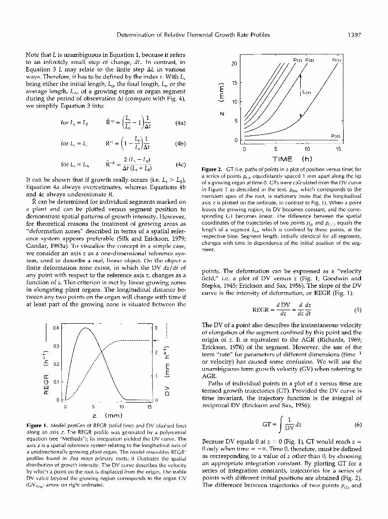
Figure 1 . Model profiles of RECR (solid line) and DV (dashed line) along an axis z. The REGR profile was generated by a polynomial equation (see “Methods”); i t s integration yielded the DV curve. The axis z i s a spatial reference system relating to the longitudinal axis of a unidirectionally growing plant organ. The model resembles REGR’ profiles found in Zea mays primary roots; it illustrates the spatial distribution of growth intensity. The DV curve describes the velocity by which a point on the root is displaced from the origin. The stable D V value beyond the growing region corresponds to the organ GV (GV,,,; arrow on right ordinate).

20

- 15 E E

10 v

N 5

O O 5 10 15

TIME (h) Figure 2. GT (i.e. paths of points in a plot of position versus time) for a series of points p( , ) , equidistantly spaced 1 mm apart along the tip of a growing organ at time O. GTs were calculated from the DV curve in Figure 1 as described in the text. p(,,,, which corresponds to the meristem apex of the root, is stationary (note that the longitudinal axis z is plotted on the ordinate, in contrast to Fig. 1). When a point leaves the growing region, its DV becomes constant, and the corresponding GT becomes linear. The difference between the spatial coordinates of the trajectories of two points p( , ) and p(,.,) equals the length of a segment L , , , , which is confined by these points, at the respective time. Segment length, initially identical for all segments, changes with time in dependence of the initial position of the segment.

points. The deformation can be expressed as a ”velocity field,” i.e. a plot of D V versus z (Fig. 1; Goodwin and Stepka, 1945; Erickson and Sax, 1956). The slope of the D V curve is the intensity of deformation, or REGR (Fig. 1):

(5)

The D V of a point also describes the instantaneous velocity of elongation of the segment confined by this point and the origin of z . It is equivalent to the AGR (Richards, 1969; Erickson, 1976) of the segment. However, the use of the term ”rate” for parameters of different dimensions (time-’ or velocity) has caused some confusion. We will use the unambiguous term growth velocity (GV) when referring to AGR.

Paths of individual points in a plot of z versus time are termed growth trajectories (GT). Provided the D V curve is time invariant, the trajectory function is the integral of reciproca1 D V (Erickson and Sax, 1956):

1 GT = \E dz

Because D V equals O at z = O (Fig. l), GT would reach z = O only when time = -a. Time O, therefore, must be defined as corresponding to a value of z other than O, by choosing an appropriate integration constant. By plotting GT for a series of integration constants, trajectories for a series of points with different initial positions are obtained (Fig. 2). The difference between trajectories of two points p ( i ) and

1398 Peters and Bernstein Plant Physiol. Vol. 11 3 , 1997

p(i-l) corresponds to the length of the segment confined by these points, L(i). Figure 3 shows a series of L(i) plotted versus time, each calculated from a pair of trajectories given in Figure 2. It cannot be emphasized enough that the validity of point trajectory and segment length calculations depends critically on the assumption of time-invariance of the DV profile.

For reasons given above, empirical REGR values can only be estimates; we will indicate their approximate character by denoting them as REGR’. To experimentally establish REGR‘ profiles, one has to start from measurements of point displacements (Fig. 4). At a given time a point p ( i ) is characterized by its longitudinal coordinate ~ ( p ( ~ ) ) . The average DV of a point, DV(p,,,), during an interval At is given by

(7)

where indices O and t denote the start and end of At, respectively (Fig. 4). Regression analysis can be applied to DV plotted versus z . The REGR’ profile then can be determined as the derivative of the regression function (Erick- son and Sax, 1956; Erickson, 1976; Zhong and Lauchli, 1993).

As an alternative to using the axis z as a reference, the movement of each point can be described relative to a neighboring one. This amounts to a description of organ growth in terms of changes of of a series of individual segments. Although can be defined by the positions of the confining points with reference to z (Eq. 8; compare

h

E v E 5

L 4 I

Z W 1 3 I- Z w 2 I (I

c n 1 W

O 2 4 6

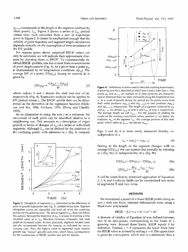
TIME (h) Figure 3. Elongation of segments L,,,, calculated as the difference of pairs of growth trajectories (see Fig. 2), plotted versus time. Segment elongation curves are sigmoidal and leve1 off when the confining points exit the growing zone. The apical segment Lo, does not follow this pattern, because the trajectory of p,o, is unique in retaining a time invariant value of z. Lo, therefore increases constantly (see inset graph at increased scale). As time proceeds, segments located more apically successively become the longest, as indicated by curves crossing over. Thus, the highest value of segmental mean relative growth rate “moves” apically with time, which bears consequences for the construction of REGR’ profiles (see text for details).

Z

Z(P(i) ,O)

z(Pli-j),t)

O

TIME O I- At

4 Figure 4. Definitions of terms used to describe marking experiments. A growing root tip is sketched at initial time O and a later time t. Two points p,il and p ( , - , ) are marked on it; their positions are characterized as distances from the apex, measured along the longitudinal axis z. As a result of growth during the period At, the points move from their initial positions ~ ( p , , , , ~ ) and ~ ( p ( , - ~ ) ; ~ ) to new positions z(p& and ~ ( p + ~ ) , ~ ) , respectively. The length of a segment confined by p(il and p(i-l), we denote L,,),o at time O and L,i),t at time t, respectively. The average length we cal1 L(i),A . For the purpose of plotting the results of the marking experiment versus position z, we define the midpoint rqi, of the segment L(i). The average position of this midpoint, which refers to L,il,A, we denote r r ~ ( ~ ) , ~ .

Figs. 2 and 4), it is more easily measured directly, i.e. independent of z.

(8)

During At the length of the segment changes with an average GV(L(,,). We can express this formally by referring to z (Eq. 9a), or independently of z, (Eq. 9b).

L(1) = Z(P(l)) - Z(P(1-1))

It will be noted that by combined application of Equations 2, 7, 8, and 9 velocity fields can be transformed into series of segmenta1 l? and vice versa.

METHODS

We formulated a model of a linear REGR profile along an axis z with one finite, terminal deformation zone, using a third-order polynomial

(10)

A domain of validity of Equation 10 was defined between two of its zero-points, corresponding to the limits of a growing zone. Beyond these limits, REGR equals O by definition. Position z = O represents the lower limit; here the REGR value is defined by setting a = O. The upper limit is given by a zero-point, which also is a minimum; thus a

REGR = f( z ) = a + bz + cz2 + dz3


smooth transition from the growing zone (domain of validity of Eq. 10) to the nongrowing region is ensured. For the purpose of the present study the model would not necessarily have to be similar to any empirical REGR’ profile. However, to emphasize the study’s practical rele- vance, constants were adjusted to let the model resemble the REGR’ profile found in Zea mays L. primary roots (Erickson and Sax, 1956; Pahlavian and Silk, 1988; Sharp et al., 1988; Pritchard et al., 1993). The model is shown in Figure 1; the coefficients are a = O, b = 0.24409 (rounded), c = -0.04419, and d = 0.002.

Algebraic integration of the REGR profile gave the DV profile (Fig. 1). Likewise, the trajectory function was found by algebraic integration (integral from Weast and Astle [1982]) of the reciproca1 DV function. Trajectories were calculated for initial positions between 1 and 15 mm in 0.0625-mm steps (examples shown in Fig. 2), and were used to calculate time-dependent changes of segment length for six initial segment sizes between 0.0625 and 2 mm, and for eight time intervals between 0.1 and 9 h. From these data segmental R were calculated for the 48 combi- nations of initial segment length and measurement duration using published methods as specified. Segmenta1 R were plotted versus segment position. The resulting REGR’ profiles were compared with the theoretical REGR curve, from which the elongation data had been derived. For qualitative comparison computer-made splines (”smooth free-hand curves”) were plotted to fit the REGR‘ data. For quantitative comparison sixth-order polynomial regression analysis was calculated for the REGR’ profiles, and deviations of four descriptive parameters were determined: (a) position of the peak, as calculated from the first derivative of the regression function; (b) REGR’ value at the peak, as calculated directly from the regression function; (c) organ GV, calculated as the definite integral of the regression function, limited by position z = O and position z of the first positive zero-point of the function; and (d) growing zone length, given by position z of the first positive zero-point of the function.

Alternatively, trajectories were used to calculate point displacements for given time intervals, and DVs for individual points were determined. Various types of regression analysis were applied to plots of DV versus z. The resulting functions were differentiated to yield REGR‘ profiles.

Calculations, plotting of functions, and statistical analyses were carried out using standard software, such as QuattroPro (version 3.00, Borland, Cambridge, UK), FigP (version 6.0c, Biosoft, Cambridge, UK), and SigmaPlot (version 5.00, Jandel, San Rafael, CA).

RESULTS AND DISCUSSION

Peak Shifts and “REGR’-Compounding”

There are only a few published comments on the nature and magnitude of systematic errors involved in various methods of REGR’ profile determination. In a study on Phleum pratense L. root growing zones, Goodwin and Avers (1956) reported that the peak position of the estimated REGR’ profile was shifted toward the apex when

long (>0.5 h) durations of measurements (At) were employed. Moreover, REGR’ values appeared to increase with increasing At. Erickson and Silk (1980; reproduced in Silk, 1984) demonstrated the same effects. They suggested that both the shift of the peak toward the apex and the increase of REGR’ peak values were caused by unsuitably long At and inappropriately great initial distances between marks. Similarly, Paolillo and Sorrells (1992) raised the question of whether REGR’ profiles derived from segmental R could generally be affected by ”technical deficiencies in the reporting and analysis of data derived from marking experiments.“ They argued that the combined effect of the time-dependent overestimation of REGR values, which they termed “REGR’-compounding,” together with the movement of segments out of the growing region in long-term experiments, could actually create false peaks.

However, one may doubt whether the above arguments apply to marking experiments in general. First, it is intuitively evident that the average growth intensity in a segment moving along a growth intensity gradient cannot possibly be greater than the highest intensity occurring in this gradient. It follows that any systematic overestimation of segmental R in marking experiments, such as ”REGR’- compounding” in the sense of Paolillo and Sorrells (1992), can only be due to inconsistent methods of R calculation. Moreover, if At increases, the period during which a segment is localized at or near a peak of growth intensity shortens relative to the whole period. We would therefore rather expect REGR’ to underestimate true REGR peak values with increasing At. Second, it remains unclear how an acropetal shift of the REGR’ profile peak could occur as a result of increased At. During a marking experiment, as is schematically presented in Figure 4, marked segments change their position on the axis. The average R, by which a segment grows during the period At, obviously corresponds to the growth intensity averaged over the whole distance the segment traverses during At. It therefore appears plausible to choose the segment’s average midpoint, m(i),A (Fig. 4) as the “segment position” when plotting segmental R versus z (Chen, 1973; Green, 1976). Notably, average midpoints W Z ( , ) , ~ trave1 away from the meristem with time. We would therefore expect the peak of the REGR‘ profile to move away from the meristem instead of toward it when At increases.

The above arguments were tested. Displacement data provided by our model for points initially spaced at 0.25-mm intervals along the axis were used to calculate segment length changes for a variety of measurement durations. We then calculated segmental R by Equation 2. To obtain REGR’ profiles, segmental R were plotted versus z, with either the initial midpoints m(i,,o (Fig. 5A), or the average segment midpoints m(i),A (Fig. 5B) defining segment position. In Figure 5A the peak indeed is seen to shift toward the meristem tip with increasing At. This is because during an experiment, more apical segments successively become the longest (compare with Fig. 3), and therefore have the highest value at the respective time. Thus, the apparent peak will move toward the meristem if the move-


0.4

0.3

l-

I 02 c v

0.1

(3 W

o' 0.4 LT 0 a

a o

0.3

02

0.1

O

O 5 10 15

Segmental plotted versus initial

midpoints m(,,,o

I I

I I

I I

Segmental E plotted versus average midpoints m,,),A

O 5 10 15

- z (mm) Figure 5. REGR' profiles obtained by plotting mean segmental relative growth rates (R; calculated for various durations of measurement between 0.25 and 9 h as indicated, with constant initial segment length 0.25 mm) versus z. Segment position was determined as the initial midpoint m(i,,o in A, and as the average midpoint m(i),A in B. In both plots the true REGR profile is indicated by the dashed line. Solid lines are computer-made free-hand fits. Original datapoints are plotted for one curve in both A and B to give an impression of the accuracy of fit; datapoints of other curves were omitted for clarity. Peak shifts and changes in apparent growing zone width occur time-dependently in both plots, but in opposite sense. A better fit is achieved when plotting data as in B (compare e.g. the curves for A t =

1 h).

ment of the segments during the period At is not accounted for. Figure 5B demonstrates how to minimize the problem by plotting segmental R versus average segment midpoints. As we expected, the peak shifts away from the meristem with time. However, the magnitude of shifting of the peak is much lower in Figure 5B if compared with Figure 5A. In the following, a11 estimated REGR' profiles are therefore produced by plotting segmental R versus average segment midpoints.

In accord with the expectations formulated above, the true peak value is increasingly underestimated with increasing At (Fig. 5). "REGR'-compounding" (as defined by Paolillo and Sorrells, 1992) does not occur. However, if one of the versions of Equation 4 is used to estimate segmental R values, the situation is different. Figure 6 shows R", E", and RtA, respectively, plotted versus R. Rt0 overestimates R depending on both At and, in a nonlinear fashion, on R itself (Fig. 6A). Identical characteristics with altered signs

apply to the underestimation of R by R't (Fig. 6B), and, to a lesser extent, to R'A (Fig. 6C). Such effects do not occur when R is plotted versus R in the same manner, for obvious reasons (if R does not change with time, both parameters are identical; Eqs. 1 and 2).

"REGR'-compounding" as a result of plotting l?" versus segment position is demonstrated in Figure 7. It is not entirely clear from the literature whether the notion that increased At inevitably leads to overestimations of REGR values (i.e. REGR'-compounding) in marking experiments is based on the inappropriate application of Equation 4a. Our analysis, however, suggests this.

0.7

0.6

O5

7 0.4 L

0.3

o2

0.1

O

n

v

0.5

0.4

0.3

02

0.1

O

O 0.1 O2 0.3 0.4 O 5

O 0.1 O 2 0.3 0.4 0.5

R (h-')

Figure 6. A, Overestimation of R by R'' (Eq. 4a). R", Calculated for uni t length elements growing at constant R for 0.5, 1, 2, and 3 h, respectively, is plotted versus R (solid lines); the bold, dashed line represents complete agreement (Rfo = R). The overestimation of R increases with the duration of measurement. The relative overestimation is dependent o n R in a nonlinear manner; fine dashed lines show deviations in percent of the actual R (only given for 0.5 and 1 h) . 6, Underestimation of R by R" (Eq. 4b); details as in A. The curves are mirror images of the ones shown in A. C, RrA (Eq. 4c)for At of 2, 4, and 6 h plotted versus R. Details as described for A. R f A underestimates R, depending on t h e measurement duration and the actual R value. The underestimation for a particular measurement duration and R value is notas severe as it is with R " (6).


0.6

O 5

0.4

O 3

O2

0.1

O O 5 10 15

z (mm) Figure 7. The phenomenon of “REGR’-compounding.” Elongation data of segments initially 0.25 mm long were calculated from our model for measurement durations of 0.5, 1, and 2 h, respectively. R t 0 of the segments was calculated and plotted versus position given by average segment midpoints (open symbols). The effects characterized in Figure 6A lead to the distortions of the profile compared with the true one, which is plotted as a solid line. The time-dependent overestimation of RECR has been termed ”REGR’-compounding.” For comparison, R calculated for the segment elongation data for 2 h duration of measurement is also plotted (solid circles); no ”REGR’- compounding” is evident in this case.

Quantification of Errors

From the above discussion we infer the following: (a) Segmental should be calculated as true mean values (Eq. 2). This follows from mathematical reasoning (Fisher, 1920; Williams, 1946), but apparently has been overlooked occasionally (compare Radford, 1967). (b) Segmental R should be plotted versus average segmental midpoints to minimize shifts of the REGR’ profile’s peak. Our analysis thus corroborates earlier suggestions by Green (1976).

Even if REGR’ profiles are produced from segmental R as suggested, some systematic error is unavoidable. Figure 8 characterizes the dependence of systematic errors on initial segment length (L,) and duration of measurement (At). REGR’ profiles were calculated from segment length data generated by our model (see ”Methods” for details). Deviations from the true profile of these estimations are expressed as the relative deviation of peak position, peak value, growing zone length, and organ GV. Intuitively, one would expect errors to increase with both initial segment length and At. This is indeed the case with peak value (Fig. 8A) and growing zone length (Fig. 88). The latter shows the greatest relative deviation of all parameters considered (see Fig. 5B for an example of the significant increase of apparent growing zone length, particularly at high Af). In contrast, deviations from the true value of estimates of organ GV show influences of two opposite tendencies (Fig. 8C). The value is decreased by the lowering of the apparent peak, particularly at high initial segment length (compare Fig. 8A). On the other hand, it is increased by the apparent

lengthening of the growing zone (compare Fig. 8C), especially at long measurement durations.

The shape of the graph of deviation of peak position (Fig. 8D) calls for an explanation. One has to recall that the shift of the apparent peak away from the apex is due to the movement of average segment midpoints that define segment position in the plots. DV of any average segment midpoint obviously equals the mean of the DV of the two points confining the segment (see Fig. 4). This implies that the average midpoint of the first segment (L(l); compare

1 PEAK VALUEI IGROWING ZONE LENGTHI

C I D

ORGAN GROWTH VELOCITY IPEAK P O S I T I O N ~

Figure 8. Quantitative comparison of the model REGR profile with REGR’ profiles estimated from segmental Ü, calculated from point displacement data generated by the model. Segmental R was calculated by Equation 2 and was plotted versus segment position defined by average segment midpoints m(,),A. Sixth-order polynomial regression was applied to yield REGR’ profiles. Deviations of four descriptive curve parameters were calculated as described in ”Methods” and plotted versus initial segment length and measurement duration (A- D). Note different scales of axes. A, The peak value of the REGR’ profile diverges less than 1 % from the true value with initial segment lengths not exceeding 1 mm, and durations of measurement of 1 h or less. Beyond these limits, the error dramatically increases. 6, Over- estimation of growing zone length depends on both initial segment length and duration of measurement over the whole range tested. The relative dependency of the deviation on measurement duration is somewhat stronger than on initial segment length. C, Organ CV is overestimated the more the longer the duration of measurement is. This effect is due to the dramatic rise of apparent growing zone length when measurement durations increase (see B). The decrease of the estimated growth velocities with increasing initial segment length is caused by the underestimation of the peak value under these conditions (see A). D, Deviation of peak position of REGR’ profiles from the position in the true RECR profile is given as per- centage of the growing zone length (true value). Deviations were small (<1%) for initial segment length not exceeding 1 mm and durations of measurements less than 2 h. The decrease in relative error in long-term measurements with high initial segment length is due to increased influence of the first segment on the form of the regression curve; for details, see text.

1402 Peters and Bernstein, Plant Physiol. Vol. 11 3 , 1997

Fig. 2) will always move slower than any other, because one of its confining points (i.e. the apex) is stationary by definition. As with time the first segment becomes longer relative to the other segments (see Fig. 3), it gains influ- ente on the position of the peak in the regression analysis. Eventually it "pulls back" the peak toward the apex to some extent, because it lags behind the movement of all other segments. Thus, the peak shift away from the apex is partly reversed, as seen in Figure 8D.

Figure 8 shows that the suggested method of REGR' profile estimation applied to data generated by the model "root" yields acceptable results for a surprisingly wide range of experimental conditions. An initial segment length of 1 mm and a measurement duration of 1 h would appear to be "sufficiently instantaneous and elemental" (Erickson and Silk, 1980); once these values are exceeded, the profile becomes unacceptably distorted. Fortunately, the values are easily met in real experimental protocols (e.g. Silk et al., 1984). However, it must not be dismissed that naked numerical values bear meaning only in the context of the analytical methods we employed. If, for example, types of regression analysis other than the sixth- order polynomial we used would be applied to the plots of segmenta1 R versus z , slightly different figures would result. Nevertheless, the general conclusion would remain.

One might be tempted to express the sufficient conditions for reliable data to result from the method applied to our model (i.e. L(i),o I 1 mm and Af 5 1 h) in more general terms. For example, one would conclude that the method works nicely as long as the initial segment length is less than 10% of the length of the whole growing zone, and the duration of measurement does not exceed the time re- quired for roughly 20% of the initial growing zone to be displaced past the growing zone boundary. It would follow

that results from experiments in which these values are exceeded are probably meaningless. Although this might be an acceptable rule of thumb in the case of profiles that resemble our model, it has to be remembered that signifi- cantly narrower margins might be applicable in other cases.

Differentiation of the Velocity Field

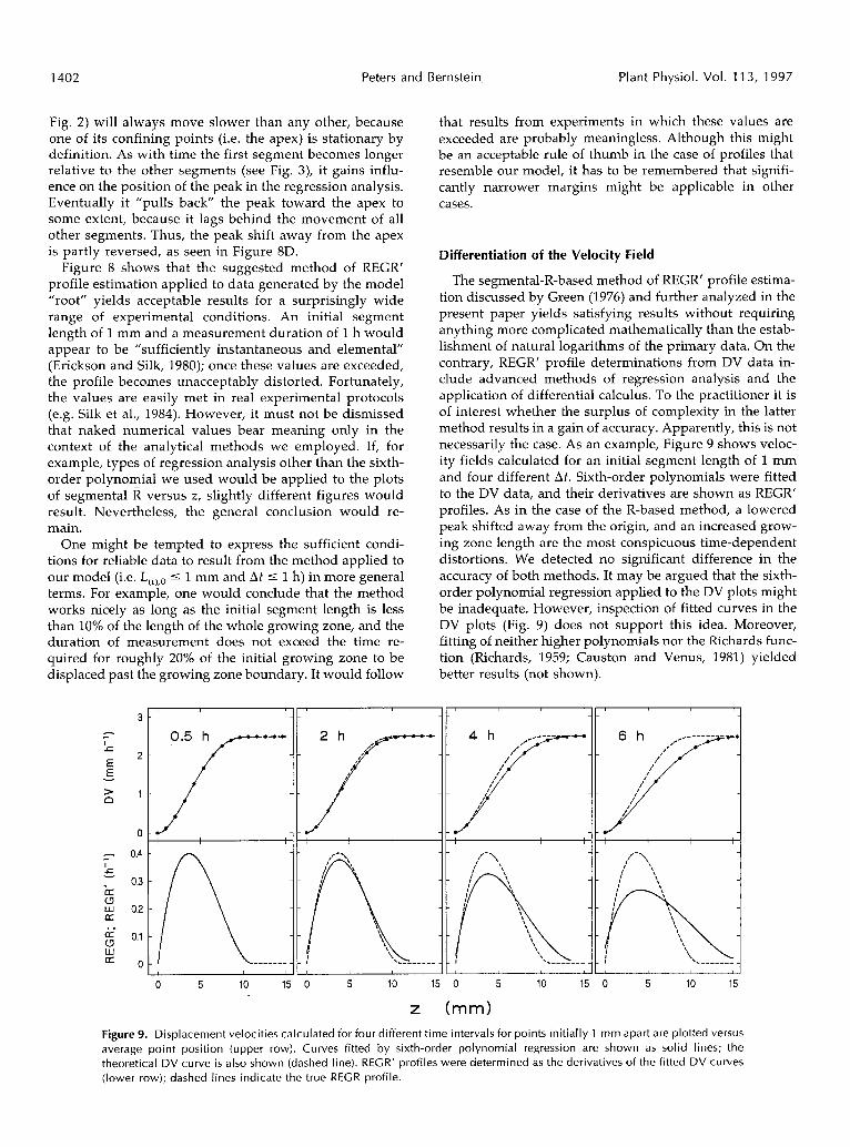
The segmental-R-based method of REGR' profile estimation discussed by Green (1976) and further analyzed in the present paper yields satisfying results without requiring anything more complicated mathematically than the establishment of natural logarithms of the primary data. On the contrary, REGR' profile determinations from DV data in- clude advanced methods of regression analysis and the application of differential calculus. To the practitioner it is of interest whether the surplus of complexity in the latter method results in a gain of accuracy. Apparently, this is not necessarily the case. As an example, Figure 9 shows velocity fields calculated for an initial segment length of 1 mm and four different Af. Sixth-order polynomials were fitted to the DV data, and their derivatives are shown as REGR' profiles. As in the case of the R-based method, a lowered peak shifted away from the origin, and an increased growing zone length are the most conspicuous time-dependent distortions. We detected no significant difference in the accuracy of both methods. It may be argued that the sixth- order polynomial regression applied to the DV plots might be inadequate. However, inspection of fitted curves in the DV plots (Fig. 9) does not support this idea. Moreover, fitting of neither higher polynomials nor the Richards function (Richards, 1959; Causton and Venus, 1981) yielded better results (not shown).

3 - r

I c 2 E

E - z 1

O

- 0.4 I c - 0.3 cf u w 02 cf

0.1 .. W c f o

O 5 10 15 O 5 10 15 O 5 10 15 O 5 10 15

z (mm) Figure 9. Displacement velocities calculated for four different time intervals for points initially 1 mm apart are plotted versus average point position (upper row). Curves fitted by sixth-order polynomial regression are shown as solid lines; the theoretical DV curve is also shown (dashed line). RECR' profiles were determined as the derivatives of the fitted DV curves (lower row); dashed lines indicate the t rue RECR profile.

Determination of Relative Elemental Crowth Rate Profiles 1403

CONCLUSIONS

Three conclusions can be reached. First, the practical significance of the distinction between spatial and material reference systems (Gandar, 1983b) appears to have been overestimated, as far as the reconstruction of spatial growth patterns is concerned. Second, problems such as ”REGR‘-compounding” (Paolillo and Sorrells, 1992), occasionally ascribed to methodological deficiencies of marking experiments in general, are avoided if appropriate numerical methods are applied. Third, the claim that any determination of REGR‘ profiles is based on measurements of displacement velocities (Silk, 1984) must not be miscon- strued to mean that ”correct” REGR’ profiles are only found by differentiation of the velocity field. Segmenta1 growth can be quantified formally both dependently and independently of the displacement velocities of the two points confining the segment. Transformation of a velocity field into a series of segment elongation data and vice versa thus is merely an arithmetical act. There is no need to go through the often cumbersome procedure of regression and differentiation of the velocity field when a less complicated technique based on segmental growth measurements is available.

Our study suggests that the method advocated by Green (1976), which consists simply of plotting segmental R versus average segment midpoints, represents such an alternative. Its value as a mathematically simple standard technique can be further increased by routinely including the following additional checks for accuracy. The most pro- nounced systematic error occurring with this method is probably the overestimation of the growing zone length (Fig. 7). The same primary data that was used to estimate the REGR’ profiles may also be plotted as segmental length increments versus initial segment position. Such increment plots are accurate regarding the growing zone length (Sachs, 1874b), and thus allow an assessment of the reliability of the REGR’ profile. A more complicated test for accuracy can be based on the average organ GV (GV,,,; see Fig. 1) during the duration of the experiment. This parameter can be measured independently; it equals the definite integral of the REGR profile along the growing zone. Significant differences between the values would indicate serious analytical errors.

In the present study we tested the reliability of methods of REGR profile estimation using a simple, theoretical model. Such models allow a quantification of systematic errors involved in the procedure of REGR’ profile determination. An experimenter may decide for maximum acceptable systematic errors, depending on the variance of data in real experiments. In this case a model facilitates the definition of experimental protocols under which these demands are met. However, a number of serious problems still remain unsolved. For example, secondary features of REGR‘ profiles, such as shoulders, secondary peaks, etc., have repeatedly been described (e.g. Goodwin, 1972; Salamon et al., 1973). It will be of interest to see under which conditions any of the different methods reliably detects secondary features of the ”true” profile, and how these can be distinguished from random error. We suspect

that a method based on segmental R will prove superior in detecting profile shoulders and secondary peaks; in the velocity field secondary features appear only as slight changes of slope, and thus might fall victim to the ”poor human perception of slope and slope change” (Silk, 1984). A test of this hypothesis will also require a characterization of the methods’ stability against statistical variance in primary data from real measurements. Studies aiming to solve these problems by using more complex models are in progress.

ACKNOWLEDGMENTS

We wish to thank Avihai Hadad for critica1 discussion during early stages of this project, Wendy Silk and Francois Tardieu for helpful remarks on a poster version of this paper, and Robert Sharp for constructive suggestions on an earlier version of the manuscript.

Received August 6, 1996; accepted January 7, 1997. Copyright Clearance Center: 0032-0889/ 97/ 113 / 1395/ 10.

LITERATURE ClTED

Barlow PW, Rathfelder EL (1985) Distribution and redistribution of extension growth along vertical and horizontal gravireacting maize roots. Planta 165: 134-141

Ben-Haj-Salah H, Tardieu F (1995) Temperature affects expansion rate of maize leaves without change in spatial distribution of cell length. Plant Physiol 109: 861-870

Berg AR, MacDonald IR, Hart JW, Gordon DC (1986) Relative elemental elongation rates in the etiolated hypocotyl of sun- flower (ffelianthus annuus L.): a comparison of straight growth and gravitropic growth. Bot Gaz 147: 373-382

Bernstein N, Lauchli A, Silk WK (1993a) Kinematics and dynam- ics of sorghum (Sorghum bicolor L.) leaf development at various Na/Ca salinities. Plant Physiol 103: 1107-1114

Bernstein N, Silk WK, Lauchli A (1993b) Growth and development of sorghum leaves under conditions of NaCl stress. Planta 191: 433439

Bernstein N, Silk WK, Lauchli A (1995) Growth and development of sorghum leaves under conditions of NaCl stress: possible role of some mineral elements in growth inhibition. Planta 1 9 6

Blackman VH (1919) The compound interest law and plant growth. Ann Bot 33: 353-360

Brumfield RT (1942) Cell growth and division in living root meristems. Am J Bot 29: 533-543

Causton DR, Venus JC (1981) The Biometry of Plant Growth. Edward Arnold, London

Chen JCW (1973) The kinetics of tip growth in the Nitella rhizoid. Plant Cell Physiol 14: 631-640

Erickson RO (1966) Relative elemental rates and anisotropy of growth in area: a computer programme. J Exp Bot 17: 390403

Erickson RO (1976) Modeling of plant growth. Annu Rev Plant Physiol 27: 407434

Erickson RO, Sax KB (1956) Elemental growth rates of the primary root of Zea mays. Proc Am Phil SOC 100: 487498

Erickson RO, Silk WK (1980) The kinematics of plant growth. Sci Amer 242: 134-151

Esau K (1943) Ontogeny of the vascular bundle in Zea mays. Hilgardia 15: 327-368

Evans GC (1972) The Quantitative Analysis of Growth. Blackwell Scientific Publications, Oxford

Feng Y, Boersma L (1995) Kinematics of axial plant growth. J Theor Biol 174: 109-117

699-705


Fisher RA (1920) Some remarks on the methods formulated in a recent article on "The quantitative analysis of plant growth." Ann Appl Biol 7: 367- 372

Gandar PW (1980) The analysis of growth and cell production in root apices. Bot Gaz 141: 131-138

Gandar PW (1983a) Growth in root apices. I. The kinematic description of growth. Bot Gaz 144: 1-10

Gandar PW (1983b) Growth in root apices. 11. Deformation and rate of deformation. Bot Gaz 144: 11-19

Goodwin RH (1972) Studies on roots. V. Effects of indoleacetic acid on the standard root growth pattern of Pkleum pratense. Bot Gaz 133: 224-229

Goodwin RH, Avers CJ (1956) Studies on roots. 111. An analysis of root growth in Pkleum pratense using photomicrographic records. Am J Bot 43: 479-487

Goodwin RH, Stepka W (1945) Growth and differentiation in the root tip of Pkleum pratense. Am J Bot 32: 36-46

Green PB (1965) Pathways of cellular morphogenesis: A diversity in Nitella. J Cell Biol 27: 343-363

Green PB (1976) Growth and cell pattern formation on an axis: critique of concepts, terminology, and modes of study. Bot Gaz

Hales S (1961) Vegetable Staticks. Beaverbrook Newspapers Ltd., London, W. and J. Innys, London, 1727. Reprint

Hunt R (1979) Plant growth analysis: the rationale behind the use of the fitted mathematical function. Ann Bot 43: 245-249

Hunt R (1982) Plant Growth Curves. Edward Arnold, London Ishikawa H, Hasenstein KH, Evans ML (1991) Computer-based

video digitizer analysis of surface extension in maize roots. Planta 183: 381-390

Lockhart JA (1971) An interpretation of cell growth curves. Plant Physiol 48: 245-248

MacAdam JW, Nelson CJ, Sharp RE (1992) Peroxidase activity in the leaf elongation zone of tall fescue. I. Spatial distribution of ionically bound peroxidase activity in genotypes differing in length of the elongation zone. Plant Physiol 99: 872-878

Morris AK, Silk WK (1992) Use of a flexible logistic function to describe axial growth of plants. Bull Math Biol 54: 1069-1081

Ohlert E (1837) Einige Bemerkungen ueber die Wurzelfasern der hoheren Pflanzen. Linnaea 11: 609-631

Pahlavanian AM, Silk WK (1988) Effect of temperature on spatial and temporal aspects of growth in the primary maize root. Plant Physiol 87: 529-532

Paolillo DJ, Rubin G (1991) Relative elemental rates of elongation and the protoxylem-metaxylem transition in hypocotyls of soy- bean seedlings. Am J Bot 78: 845-854

Paolillo DJ, Sorrells ME (1992) The spatial distribution of growth in the extension zone of seedling wheat leaves. Ann Bot 70: 461470

Pilet PE, Senn A (1980) Root growth gradients: a critica1 analysis. Zeitschr Pflanzenphys 99: 121-130

Poorter H (1989) Plant growth analysis: towards a synthesis of the classical and the functional approach. Physiol Plant 75: 237-244

Poorter H, Garnier E (1996) Plant growth analysis: an evaluation of experimental design and computational methods. J Exp Bot

Pritchard J, Hetherington PR, Fry SC, Tomos AD (1993) Xyloglu- can endotransglycosylase activity, microfibril orientation and the profiles of cell wall properties along growing regions of maize roots. J Exp Bot 44: 1281-1289

Radford PJ (1967) Growth analysis formulae: their use and abuse. Crop Sci 7: 171-175

137: 187-202

47: 1343-1351

Richards FJ (1959) A flexible growth function for empirical use. J

Richards FJ (1969) The quantitative analysis of growth. In FC Stew- ard, ed, Plant Physiology. Academic Press, New York, pp 3-76

Richards OW, Kavanagh AJ (1943) The analysis of the relative growth gradients and changing form of growing organisms: illustrated by the tobacco leaf. Am Nat 77: 385-399

Saab IN, Sharp RE, Pritchard J (1992) Effect of inhibition of abscisic acid accumulation on the spatial distribution of elongation in the primary root and mesocotyl of maize at low water potentials. Plant Physiol 99: 26-33

Sachs J (1874a) Ueber den Einfluss der Lufttemperatur und des Tageslichts auf die stündlichen und taglichen Aenderungen des Langenwachsthums (Streckung) der Internodien. Arbeiten Bot Inst Wiirzburg 1: 99-192

Sachs J (187413) Ueber das Wachsthum der Haupt- und Neben- wurzeln. Arbeiten Bot Inst Wiirzburg 1: 385-474

Salamon P, List A, Grenetz PS (1973) Mathematical analysis of plant growth. Zea mays primary roots. Plant Physiol51: 635-640

Schnyder H, Nelson CJ (1988) Diurnal growth of tall fescue leaf blades. I. Spatial distribution of growth, deposition of water, and assimilate import in the elongation zone. Plant Physiol 86: 1070- 1076

Schnyder H, Nelson CJ, Spollen WG (1988) Diurnal growth of tall fescue leaf blades. 11. Dry matter partitioning and carbohydrate metabolism in the elongation zone and adjacent expanded tissue. Plant Physiol 86: 1077-1083

Sharp RE, Silk WK, Hsiao TC (1988) Growth of the maize primary root at low water potentials. I. Spatial distribution of expansive growth. Plant Physiol 87: 50-57

Silk WK (1984) Quantitative description of development. Annu Rev Plant Physiol35: 479-518

Silk WK (1989) Growth rate patterns which maintain a helical tissue tube. J Theor Biol 138: 311-327

Silk WK, Abou Haidar S (1986) Growth of the stem of Pharbitis nil: analysis of longitudinal and radial components. Physiol Vég 24:

Silk WK, Erickson RO (1978) Kinematics of hypocotyl curvature. Amer J Bot 65: 310-319

Silk WK, Erickson RO (1979) Kinematics of plant growth. J Theor Biol 76: 481-501

Silk WK, Walker RC, Labavitch J (1984) Uronide deposition rates in the primary root of Zea mays. Plant Physiol 74: 721-726

Spollen WG, Sharp RE (1991) Spatial distribution of turgor and root growth at low water potentials. Plant Physiol 96: 438-443

Venus JC, Causton DR (1979) Plant growth analysis: a re- examination of the methods of calculation of relative growth and net assimilation rates without using fitted functions. Ann

Verse1 JM, Mayor G (1985) Gradients in maize roots: local elongation and pH. Planta 164: 96-100

Weast RC, Astle MJ eds (1982) CRC Handbook of Chemistry and Physics, Ed 63. CRC Press, Boca Raton, FL

Williams RF (1946) The physiology of plant growth with special reference to the concept of net assimilation rate. Ann Bot 10: 41-72

Wolf SD, Silk WK, Plant RE (1986) Quantitative patterns of leaf expansion: comparison of normal and malformed leaf growth in Vitis vinifevn cv. Ruby Red. Amer J Bot 73: 832-846

Zhong H, Lauchli A (1993) Spatial and temporal aspects of growth in the primary root of cotton seedlings: effects of NaCl and CaC1,. J Exp Bot 44: 763-771

EXP Bot 10: 290-300

109-116

Bot 43: 633-638

Documents

The Determination of Relative Elemental Growth Rate