The Development of a Strain-based Defect Assessment

The Development of a Strain-based

Defect Assessment Technique for

Composite Aerospace Structures

Thesis submitted in accordance with the

requirements of the University of Liverpool

for the degree of Doctor of Philosophy by

William J. R. Christian

October 2017

i

Abstract

The Development of a Strain-based Defect Assessment Technique for

Composite Aerospace Structures

By William J. R. Christian

This thesis details the work conducted over three years on the development of

strain-based defect assessment techniques for carbon-fibre reinforced composites. This

material, whilst exhibiting a high specific strength, is sensitive to defects and thus there is

an industrial need for assessment techniques that are capable of characterising defects

and obtaining predictions of residual strength or life. The most commonly applied

techniques are currently ultrasonic and thermographic non-destructive evaluation. A

strain-based defect assessment could lead to more accurate predictions of residual

strength, resulting in a reduction of the costs associated with operating composite

aerospace structures. The aim of this project is to increase the quality and confidence in

residual strength information gained from the non-destructive evaluation of composite

defects using strain-based assessments, in addition to currently applied ultrasonic

practices for composite structures. A literature review on composite defects and existing

techniques for assessing defects was conducted. Knowledge gaps were then identified

that if filled, could improve residual strength predictions.

Initially, a statistical framework was developed that used Bayesian regression to

predict the residual strength of impacted composites, based on ultrasonic non-destructive

measurements, that is robust to data outliers. As part of this framework a performance

metric for quantifying the accuracy of residual strength predictions was introduced,

allowing currently applied assessment techniques to be compared with the novel strain-

based assessment.

Then, a novel technique for performing strain-based defect assessments was

developed that utilised image decomposition and the statistical framework to make

ii

residual strength predictions. Digital image correlation was used to measure strain fields

which were then dimensionally reduced to feature vectors using image decomposition.

The difference between feature vectors representing virgin and defective laminates were

quantified, resulting in a strain-based defect severity measure. Bayesian regression was

used to fit an empirical model capable of predicting the residual strength of an impacted

laminate based on the strain-based defect severity. The accuracy of the strain-based

predictions were compared to the accuracy of ultrasound-based predictions and found to

outperform the currently applied ultrasonic technique.

Strain-based assessment of in-plane fibre-waviness was also explored, as minimal

research had been conducted studying waviness defects with full-field techniques. This

required the development of a procedure for creating controlled levels of local waviness

in laminates. The same strain-based assessment used for assessing impact damage was

applied to the fibre-waviness specimens, but for this defect the accuracy of predictions

were found to be comparable to the ultrasound-based predictions. However, residual

strain measurements were found to be effective for predicting the strength of laminates,

indicating that knowledge of the residual strains around a waviness defect may be

important when predicting a laminates residual strength.

iii

Acknowledgements

I am grateful to my supervisors, Professor Eann Patterson and Dr Alex Diaz De la O

(both of the University of Liverpool) for their guidance throughout my research project.

Their expertise and suggestions have been indispensable during the many hours I have

spent on experimental work and report drafting. I am also grateful to Jiji Mathews for his

assistance during my experimental work.

Throughout my studies I have had many useful discussions with individuals at

Airbus, in particular I would like to thank Dr Kathryn Atherton and Eszter Szigeti for all of

their helpful suggestions and industrial insight.

My research was funded by an EPSRC CASE award sponsored by Airbus and I am

grateful to both organisations for their financial support.

Finally I would like to thank my wife Beth for all the support she has given me and

my daughter Emma for providing many welcome distractions from work.

iv

Table of Contents

List of Tables ...................................................................................................................... vii

List of Figures .................................................................................................................... viii

1. Introduction .................................................................................................................... 1

1.1. Background .............................................................................................................. 1

1.2. Aim and Objectives .................................................................................................. 3

2. Literature Review ............................................................................................................ 4

2.1. Conventional Non-destructive Evaluation of Composites ....................................... 4

2.2. Robust Statistics ....................................................................................................... 6

2.3. Stress and Strain Based Defect Assessments ........................................................... 8

2.4. Image Decomposition ............................................................................................ 10

2.5. Fibre-Waviness in Composite Laminates ............................................................... 14

2.5.1. Mechanics of Waviness Defects ...................................................................... 14

2.5.2. Detection and Quantification of Waviness ..................................................... 16

2.6. Knowledge Gaps..................................................................................................... 18

3. Experimental Techniques .............................................................................................. 20

3.1. Pulse-Echo Ultrasonic Non-destructive Evaluation ............................................... 20

3.2. Digital Image Correlation ....................................................................................... 22

3.3. Thermoelastic Stress Analysis ................................................................................ 25

4. Robust Empirical Predictions of the Residual Strength of Defective Composites Based

on Ultrasound Measurements .......................................................................................... 28

4.1. Introduction ........................................................................................................... 28

4.2. Regression Techniques........................................................................................... 29

4.2.1. Classical Linear Regression .............................................................................. 29

4.2.2. Bayesian Regression ........................................................................................ 30

4.3. Experimental Method ............................................................................................ 31

v

4.4. Bayesian Modelling ................................................................................................ 33

4.4.1. Robust Bayesian Linear Regression................................................................. 33

4.4.2. Piecewise Robust Bayesian Regression ........................................................... 38

4.5. Performance Metrics ............................................................................................. 40

4.6. Results .................................................................................................................... 41

4.7. Discussion ............................................................................................................... 46

4.8. Conclusion .............................................................................................................. 52

5. Strain-based Defect Assessment of Impacted Composite Laminates .......................... 54

5.1. Introduction ........................................................................................................... 54


5.3. Strain-Based Defect Assessment ........................................................................... 56

5.4. Results .................................................................................................................... 61

5.5. Discussion ............................................................................................................... 71

5.6. Conclusions ............................................................................................................ 76

6. Manufacture and Characterisation of In-plane Fibre-waviness Defects ...................... 78

6.1. Introduction ........................................................................................................... 78


6.2.1. Fabrication of Coupons Containing Waviness Defects ................................... 79

6.2.2. Ultrasonic Characterisation ............................................................................ 81

6.2.3. Digital Image Correlation and Thermoelastic Stress Analysis of Waviness

Coupons .................................................................................................................... 82

6.3. Results .................................................................................................................... 83

6.4. Discussion ............................................................................................................... 94

6.5. Conclusions .......................................................................................................... 100

7. Discussion .................................................................................................................... 101

7.1. Creating Defects in Composite Coupons ............................................................. 101

vi

7.2. Predicting the Residual Strength of Laminates Containing Defects .................... 104

7.3. Strain-Based Defect Assessments ........................................................................ 106

7.5. Future Work ......................................................................................................... 110

8. Conclusions ................................................................................................................. 113

References ...................................................................................................................... 115

Appendix A: R Code for Bayesian Regression ................................................................. 125

Appendix B: JAGS Code for Robust Bayesian Linear Regression .................................... 127

Appendix C: JAGS Code for Piecewise Robust Bayesian Regression ............................... 128

vii

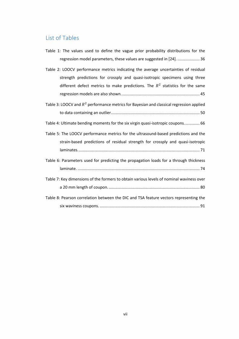
List of Tables

Table 1: The values used to define the vague prior probability distributions for the

regression model parameters, these values are suggested in [24]. .................... 36

Table 2: LOOCV performance metrics indicating the average uncertainties of residual

strength predictions for crossply and quasi-isotropic specimens using three

different defect metrics to make predictions. The 𝑅2 statistics for the same

regression models are also shown. ...................................................................... 45

Table 3: LOOCV and 𝑅2 performance metrics for Bayesian and classical regression applied

to data containing an outlier. ............................................................................... 50

Table 4: Ultimate bending moments for the six virgin quasi-isotropic coupons. ............. 66

Table 5: The LOOCV performance metrics for the ultrasound-based predictions and the

strain-based predictions of residual strength for crossply and quasi-isotropic

laminates. ............................................................................................................. 71

Table 6: Parameters used for predicting the propagation loads for a through thickness

laminate. .............................................................................................................. 74

Table 7: Key dimensions of the formers to obtain various levels of nominal waviness over

a 20 mm length of coupon. .................................................................................. 80

Table 8: Pearson correlation between the DIC and TSA feature vectors representing the

six waviness coupons. .......................................................................................... 91

viii

List of Figures

Figure 1: Ultrasound A-scan of a composite laminate at the location of a delamination,

also showing an exemplar gate. ........................................................................ 21

Figure 2: The multi-axis ultrasound C-scan machine used for this thesis. ........................ 22

Figure 3: A DIC image showing a speckle pattern applied to a specimen (top) with a

magnified image of a single facet (bottom-left) and the same facet after loading

(bottom-right). Scale bars are nominal as the specimen was viewed at an

angle. .............................................................................................................. 23

Figure 4: A third-angle projection diagram of the DIC setup showing the LED light and

camera positions (left) and bending rig (right).................................................. 24

Figure 5: A specimen under cyclic bending whilst TSA was performed. .......................... 27

Figure 6: Histogram of 5000 samples randomly distributed with a normal distribution

(with 𝜇 = 0 and 𝜎 = 1), with the probability distribution function of the normal

distribution, 𝑝(𝑦), superimposed. .................................................................... 31

Figure 7: Schematic diagram showing how the regression model (bottom) is formed from

a linear regression line with the data distributed around it in the form of a t-

distribution (middle). At the top are the initial or prior probability distributions

for the values of the model parameters. .......................................................... 35

Figure 8: Illustration of the probability density function for the t-distribution as a function

of the normality parameter ν for a mean, 𝜇 = 0 and spread, 𝜎 = 1. As ν tends

to infinity, the t-distribution converges to a normal distribution. .................... 36

Figure 9: A typical predictive distribution of residual strength, y*, as a function of

ultrasound measurement, x*, based on a Bayesian linear regression model fitted

to the measured data values (crosses) with prediction uncertainties and a 95%

credible interval. The dots on the three lines indicate the locations at which

percentiles of the predictive distribution were calculated. The lines are spline

curves interpolated through the quantified points. .......................................... 38

Figure 10: Schematic diagram showing how the basis function for piecewise robust

Bayesian regression (solid black line in the bottom graph) is formed using three

parameters and the prior distributions for those parameters (top). ................ 39

ix

Figure 11: A typical time-of-flight C-scan of impact damage in a quasi-isotropic composite

laminate, showing the defect metrics used. The defect area was defined as the

projected area of all the delaminations when viewed in the C-scan. Colour is

used to indicate the depth of delaminations from the impacted surface. ....... 41

Figure 12: Time-of-flight C-scans of quasi-isotropic coupons with increasing impact

energies of 5J, 8J, 12J and 15J. .......................................................................... 42

Figure 13: Time-of-flight C-scans of crossply coupons with increasing impact energies of

5J, 8J, 10J and 12J. ............................................................................................. 42

Figure 14: Residual strength predictions made using Bayesian linear regression for

impacted quasi-isotropic specimens using ultrasound measurements of defect

area (top), length (middle) and width (bottom) as the defect metric. The size of

the 95% credible interval (grey shading) indicates that the uncertainty is smallest

when the area of the defect was used as the defect metric which concurs with

the LOOCV performance metric data in Table 2. .............................................. 43


impacted crossply coupons using ultrasound measurements of defect area (top),

length (middle) and width (bottom) as the defect metric. ............................... 44


impacted crossply specimens using the defect area from the ultrasound

measurements as the defect metric together with the 95% credible interval

(grey shading). The dotted lines indicate an exemplar minimum residual bending

strength and the corresponding maximum allowable defect area for coupons

with a probability of failure of less than 2.5%. .................................................. 46

Figure 17: Residual strength predictions made using Bayesian linear regression for a small

set of four impacted quasi-isotropic specimens. Strength predictions were based

on ultrasound measurements of defect area. The wide light grey region is the

Bayesian regression credible interval and the narrow dark grey region is the

classical regression confidence interval. ........................................................... 48

Figure 18: Bayesian linear regression based on artificial data generated using the linear

function in equation (8) with normally distributed measurement noise. ......... 49

x

Figure 19: Classical (dashed and dotted line with dark grey shading) and Bayesian (dashed

line with light grey shading) linear regression and corresponding confidence and

credible intervals based on the artificial data in Figure 18 with the addition of an

outlier at (4, 30). ................................................................................................ 50

Figure 20: Piecewise robust Bayesian regression applied to non-continuous data

generated using equation (9). ........................................................................... 51

Figure 21: Piecewise robust Bayesian regression applied to non-continuous data

generated using equation (9) with two outliers. ............................................... 51

Figure 22: A coupon with speckle pattern applied at the location where the impact was

applied showing dimensions and the coordinate system used for the DIC and

ultrasound measurements. ............................................................................... 55

Figure 23: Coupon under four-point bend load with the cameras used for DIC attached to

the top half of the rig facing the impacted surface of the coupon. .................. 57

Figure 24: The first 120 of the 325 shape descriptors in a feature vector describing the

strain field on a loaded coupon with impact damage (left) with the filter

thresholds indicated by dashed lines. All 325 shape descriptors were used for

the unfiltered reconstruction (top right) but only 29 shape descriptors, shaded

in the bar chart, were required after filtering (bottom right). .......................... 59

Figure 25: Ultrasound time-of-flight C-scan of the delaminations formed by a 12 J impact

on a crossply laminate (top) and the corresponding surface strain field (bottom)

with the 25 mm square region used for image decomposition shown in

white. ........................................................................................................... 62

Figure 26: Ultrasound time-of-flight C-scan of the delaminations formed by a 12 J impact

on a quasi-isotropic laminate (top) and the corresponding surface strain field

(bottom) with the 25 mm square region used for image decomposition shown

in white. ............................................................................................................. 63

Figure 27: Strain fields observed in crossply coupons with increasing impact energies of

0 J, 5 J, 8 J and 10 J (reading left-to-right from top-left). .................................. 64

Figure 28: Strain fields observed in quasi-isotropic coupons with increasing impact

energies of 0 J, 5 J, 10 J and 15 J (reading left-to-right from top-left). ............. 65

xi

Figure 29: Regression models relating defect severity measurements to the residual

strength of defective crossply composites using the ultrasound-based defect

severity (top) and the Manhattan distance for strain-based

assessments (bottom). ...................................................................................... 67

Figure 30: Regression models relating defect severity measurements to the residual

strength of defective quasi-isotropic composites using the ultrasound-based

defect severity (top) and the Manhattan distance for strain-based

assessments (bottom). ...................................................................................... 68

Figure 31: Strain-based defect assessments of crossply coupons using Pearson

dissimilarity (top) and Euclidean distance (bottom). ........................................ 69

Figure 32: Strain-based defect assessments of quasi-isotropic coupons using Pearson

dissimilarity (top) and Euclidean distance (bottom). ........................................ 70

Figure 33: The moment, 𝑀𝑝, to cause propagation of a delamination (solid line) as a

function of the strain difference, ∆𝜖, relative to a virgin coupon, developed

around the delamination when an inspection moment of 20 Nm is applied

(dotted line). The graph indicates the inspection moment will not induce

propagation and the minimum measurable strain difference (dashed line)

corresponds to a delamination that will only propagate due to a moment larger

than the ultimate moment of the virgin coupon (chain line). ........................... 75

Figure 34: Photograph of a former for creating coupons with a nominal waviness

of 15%. ........................................................................................................... 80

Figure 35: Photograph of a coupon with a nominal waviness of 25%, showing the speckle

pattern and measurement coordinate system. ................................................ 81

Figure 36: A subset with applied Hann window (top) and its spectral image (bottom) taken

from an amplitude C-scan of a waviness defect in a 17.5% nominal waviness

coupon. .............................................................................................................. 82

Figure 37: DIC measurements of the surface deviation from a flat plane for an unloaded

coupon with a nominal waviness of 17.5% (top) and the associated residual

strain field (bottom). ......................................................................................... 84

xii

Figure 38: A coupon that had a nominal waviness of 25%, inspected with: ultrasound (top),

surface strain at a load of 22 Nm (middle) and residual strain measurements

(bottom). ........................................................................................................... 85

Figure 39: The ultrasound measured waviness for coupons after curing for six different

levels of nominal waviness. ............................................................................... 86

Figure 40: The effect of waviness after curing on the ultimate bending moment for all

coupons. ............................................................................................................ 87

Figure 41: Graphs for predicting the ultimate bending moment of coupons using RMS of

waviness measured with ultrasound (left) and the mean of the residual strain

field (right). ........................................................................................................ 87

Figure 42: Predictions of residual strength made using the strain-based defect assessment

technique for fibre-waviness coupons. ............................................................. 88

Figure 43: Full field maps of the thermoelastic signal for six waviness coupons. Colour is

used to show the magnitude of the thermoelastic signal in raw camera units. 89

Figure 44: DIC strain fields of fibre-waviness defects. Colour indicates the magnitude of

surface first strain invariant. ............................................................................. 90

Figure 45: Using shape descriptors (bottom) to compare a DIC measured strain fields (top-

left) and a TSA thermoelastic signal field (top-right) for the same coupon. ..... 91

Figure 46: Abaqus FE mesh of a fibre-waviness coupon during a four-point bend. ......... 92

Figure 47: Predictions of surface strain (top-left) and DIC measurements (top-right) for a

25% waviness coupon. The validation diagram (bottom) shows that the model is

valid given the uncertainty of the measurement system, the inset shows an

enlarged version of the boxed region on the main graph. ................................ 93

Figure 48: Load-displacement graph for a coupon that had a nominal waviness of 25%

loaded to failure with four points on the load curve marked (top) and the strain-

fields at these points (bottom). ......................................................................... 94

Figure 49: Strain-based defect assessment graph for impacted quasi-isotropic coupons

(crosses) with fibre-waviness data points (circles) plotted as well. .................. 98

1

1. Introduction

1.1. Background

Composite materials are used in aircraft structures to assist in reducing weight,

without compromising strength. This weight reduction allows for more efficient aircraft,

decreasing both the financial and environmental costs of air travel. Whilst composite

materials have high specific-strengths relative to the aluminium alloys they typically

replace, they are sensitive to defects. These defects can cause the ultimate strength of

the structure to be substantially lower than the intended design value. In addition to this,

the defects are often difficult to visibly locate. To account for defects that may be present

but undetected, aircraft are designed assuming that defects are always present in the

structure. Composite structures are then assessed at intervals, to ensure that material

defects that actually exist are not going to result in failure during operation. These

assessment techniques can take many forms depending on the material and defects they

are designed to detect. The importance of the information they provide can also vary

considerably. Rytter [1] categorised the information obtained from defect assessments

into four levels, which are described as follows [2]:

Level 1: Defect detection

Level 2: Level 1 plus location identification

Level 3: Level 2 plus extent definition

Level 4: Level 3 plus remnant life prediction

For composite structures there are substantial costs associated with repairs, hence it

would be beneficial for assessment techniques to provide Level 4 information. This could

help to reduce the number of repairs to those that are essential for the structure to be

safely operated. Ultrasound and thermography are amongst the most common

techniques currently employed to assess aerospace composites [3], and provide Level 3

information in the form of the size and shape of defects. From this data, the residual

strength of the structure can be inferred, but predictions based on these measurements

have high levels of uncertainty because the effect of the defect on the structural integrity

is not completely characterised [4]. In general, the loss of structural integrity involves the

failure of materials due to the breaking of bonds as a result of deformation. It is possible

to characterise this deformation in terms of strain fields. Hence, the changes in strain

2

fields induced by defects should be treated as Level 4 information in Rytter’s classification,

because they provide the most appropriate input parameters for predicting the change in

structural integrity, or residual strength [2]. Thus, employing strain fields to assess the

effect of defects in composites is likely to lead to more reliable predictions of the residual

strength or life; and in turn, likely to reduce premature or unnecessary repairs.

Techniques such as digital image correlation (DIC) and thermoelastic stress

analysis (TSA) can be used to capture full-field surface strain data to assess the integrity

of a component. This data is a suitable input for a Level 4 defect classification technique,

however the full-field data has a high level of dimensionality which must be reduced to

obtain the key information required for residual strength predictions. Patki and Patterson

[5] developed a technique of reducing the dimensionality of full-field strain data using

image decomposition. Strain fields on the surface of impacted glass-fibre laminates were

dimensionally reduced to feature vectors. The numerical dissimilarity between feature

vectors representing a virgin laminate and a defective laminate was then used as a

measure of the defect severity for the defective laminate. This thesis extends the

technique developed by Patki and Patterson to obtain residual strength predictions of

defective composites. The residual strength predictions made using strain data would be

expected to be more accurate than predictions made using conventional ultrasonic non-

destructive evaluation (NDE). To confirm this, the effectiveness of strain-based and

ultrasound-based assessments will be quantified and compared.

Defects commonly encountered in the commercial aerospace industry will be

used to demonstrate the effectiveness of the defect assessment technique. As strain-

based defect assessments have already been successfully applied to impact damage, a

common form of service damage for composite aircraft structures, this will be one of the

defects assessed using the technique. This will be the first time the technique is used to

predict residual strength, and thus, will ensure the technique is verified before applying it

to other defects. Impact events result in complicated regions of damage with

delaminations, fibre fracture and matrix cracking all present in close proximity to each

other [6] making it difficult to predict the strength of the defective composite and thus a

major concern for industry. However, despite the complexity of the defect produced by

these events, it is simple to recreate the defect in a laboratory setting. Drop-weight impact

testing [7] is a common method of creating impact damage and thus will be used in this

3

study. To demonstrate that strain-based assessments are not limited to impact damage,

a form of manufacturing defect completely distinct from impact damage will also be

explored. Cantwell and Morton [8] listed five common forms of manufacturing defect that

are encountered in industry:

Resin-rich areas

Voids

Fibre-waviness (Cantwell and Morton refer to this as, ‘distorted fibres’)

Broken fibres

Inclusions

After discussions with Airbus, the industrial sponsor of this project, it was decided that

fibre-waviness would be a suitable defect to be explored. Composite laminates are said

to contain fibre-waviness when, instead of having a uniform orientation, the fibre

orientation has local variations. This can cause the material to be weaker than the design

strength [9] and thus can lead to premature failure.

1.2. Aim and Objectives

The aim of this project is to increase the quality and confidence in residual

strength information gained from the non-destructive evaluation of composite defects

using strain-based inspections, in addition to currently applied ultrasonic practices for

composite structures. The objectives of this project are to:

develop the statistical methods for predicting the remnant properties of defective

structures based on non-destructive measurements.

develop a technique for determining the severity of defects using full-field strain-

data.

demonstrate the effectiveness of strain-based defect assessments relative to

current practices of ultrasonically inspecting aircraft.

4

2. Literature Review

This chapter is a review of the literature related to assessing defects in composite

laminates and structures. The focus of the literature review is on the assessment of impact

damage and fibre waviness. The chapter is split into six sections with the first section

focusing on methods of predicting the performance of defective composites. The second

section discussing statistics that are robust to outliers. The third section focuses on stress

and strain based techniques of assessing defects in composites and the fourth section

focusing on how image decomposition can be used as part of a strain-based NDE

technique. Literature on fibre-waviness is introduced in the fifth section and knowledge

gaps are identified in the final section.

2.1. Conventional Non-destructive Evaluation of Composites

The main focus of the NDE research community is on developing techniques to

locate defects in a structure. This thesis is concerned with predicting the behaviour of

composite structures containing defects and thus this section focuses on methods of

determining the effects of defects on remnant properties using non-destructive

measurements. In 1975, Stone and Clarke [10] demonstrated a technique for predicting

the inter-laminar shear strength of a laminate containing porosity. By controlling the

pressure used to cure flat crossply laminates in an autoclave, the void content in a

specimen was controlled. Through-transmission ultrasound was then used to measure the

ultrasound attenuation coefficient of the laminate. Finally, the inter-laminar shear

strength of the laminate was measured. A linear relation was observed between the

attenuation coefficient and the measured inter-laminar shear strength demonstrating

that the technique could be used to predict the loads at which delaminations would

initiate and then propagate in a structure.

Also in 1975, measurements of surface damage were used to predict the residual

strength of composites containing ballistic impact damage. Avery and Porter [11]

performed a series of tests on boron-fibre and carbon-fibre reinforced composites plates.

Various projectiles, which are occasionally encountered by military aircraft, were fired at

composite plates at different speeds and angles. These projectiles resulted in holes

through the plates with cracks extending from the holes. The width of the visible damage

transverse to the loading direction was measured and then the plate loaded to failure in

tension. When the visible damage width was plotted against residual strength, a linear

5

relation was observed. The method of least-squares was used to fit a line to the data and

confidence intervals were also calculated. The lower bound of these confidence intervals

could then be used to make conservative predictions of residual strength, using only

measurements of surface damage. Fifty specimens were tested, demonstrating the

effectiveness of the technique. However, the technique is irrelevant for civil aerospace as

typical forms of service damage, e.g. hail or tool drops, do not result in penetration of the

structure and often result in barely-visible impact damage [6].

In 1990, the previously described damage assessment procedure was modified by

Prichard and Hogg [12] for barely-visible impact damage. Composites plates were

manufactured using two different material systems. Both materials were reinforced by

carbon fibre but one was produced using an epoxy matrix and the other using a

polyetheretherketone (PEEK) thermoplastic matrix. Both laminates used a quasi-isotropic,

[-45\0\45\90]2S lay-up and were then impacted using a 20 mm hemispherical tup at

energies between 0 and 15 J. This resulted in twenty epoxy matrix specimens and

nineteen thermoplastic specimens. The specimens were assessed using C-scan ultrasound

and the width of the defect transverse to the intended direction of loading was recorded.

The laminates were then loaded in compression to determine the residual strength. A

correlation was observed between the residual strength and the defect width and a line-

of-best fit was determined using least-squares regression. The line-of-best-fit could be

used to make predictions of the average residual strength of a coupon for a given defect

size. A confidence interval was also calculated for the predictions, this interval could then

be used to make conservative estimates of residual strength. A high amount of variability

in the behaviour of impacted composites means that data outliers can potentially occur

[6, 13]. A method of accounting for data outliers, that might affect the parameters of the

line-of-best-fit, was suggested by Prichard and Hogg [12]. The method of maximum

normed residual [14] was used to identify if outliers were present in the dataset. It was

suggested that if outliers were identified, then these should be removed and the

regression performed on the remaining data. This assumes that the outliers are an

incorrect measurement, when they could in fact be a valid outcome when testing

laminates that contain defects. By removing outliers from the data set, the confidence

interval for predictions would likely be too small [15] resulting in predictions of residual

strength which are potentially optimistic.

6

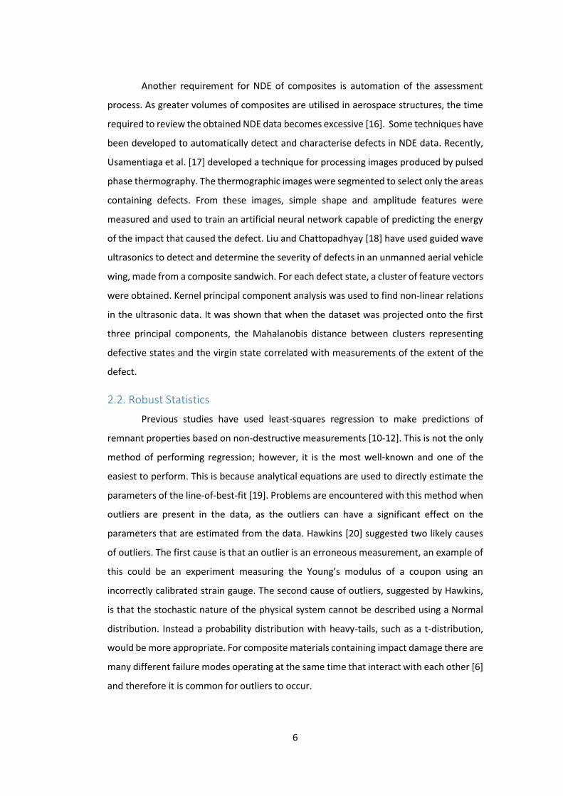
Another requirement for NDE of composites is automation of the assessment

process. As greater volumes of composites are utilised in aerospace structures, the time

required to review the obtained NDE data becomes excessive [16]. Some techniques have

been developed to automatically detect and characterise defects in NDE data. Recently,

Usamentiaga et al. [17] developed a technique for processing images produced by pulsed

phase thermography. The thermographic images were segmented to select only the areas

containing defects. From these images, simple shape and amplitude features were

measured and used to train an artificial neural network capable of predicting the energy

of the impact that caused the defect. Liu and Chattopadhyay [18] have used guided wave

ultrasonics to detect and determine the severity of defects in an unmanned aerial vehicle

wing, made from a composite sandwich. For each defect state, a cluster of feature vectors

were obtained. Kernel principal component analysis was used to find non-linear relations

in the ultrasonic data. It was shown that when the dataset was projected onto the first

three principal components, the Mahalanobis distance between clusters representing

defective states and the virgin state correlated with measurements of the extent of the

defect.

2.2. Robust Statistics

Previous studies have used least-squares regression to make predictions of

remnant properties based on non-destructive measurements [10-12]. This is not the only

method of performing regression; however, it is the most well-known and one of the

easiest to perform. This is because analytical equations are used to directly estimate the

parameters of the line-of-best-fit [19]. Problems are encountered with this method when

outliers are present in the data, as the outliers can have a significant effect on the

parameters that are estimated from the data. Hawkins [20] suggested two likely causes

of outliers. The first cause is that an outlier is an erroneous measurement, an example of

this could be an experiment measuring the Young’s modulus of a coupon using an

incorrectly calibrated strain gauge. The second cause of outliers, suggested by Hawkins,

is that the stochastic nature of the physical system cannot be described using a Normal

distribution. Instead a probability distribution with heavy-tails, such as a t-distribution,

would be more appropriate. For composite materials containing impact damage there are

many different failure modes operating at the same time that interact with each other [6]

and therefore it is common for outliers to occur.

7

One of the earliest techniques for accounting for data outliers was to identify and

remove them. Of particular note is the maximum normed residual method, developed by

Grubbs [21] and published in 1950. This technique normalises a data sample by

subtracting the mean from each value and dividing the resulting values by their standard

deviation, these are referred to as normed residuals. If the highest normed residual is

above a critical value then it is identified as an outlier and removed from the data sample.

This process is repeated until no more outliers are identified. This technique is commonly

applied to composite materials and is one of the recommended techniques for the

determination of material properties in Chapter 8 of MIL-HDBK-17-1 [14]. The method is

simple to apply, but can only be used if multiple samples with the same level of defect

severity are available.

In 1984, Rousseeuw [22] developed the method of least trimmed squares, which

was capable of performing regression with data containing outliers. Least trimmed

squares works by performing least-squares regression on subsets of the available data. A

large number of different subsets are chosen and for each fit the coefficient of

determination, 𝑅2, is calculated. The line-of-best-fit for the subset with the lowest 𝑅2 is

then chosen as the line-of-best-fit for the complete dataset. This method is robust to

outliers as the subset with the lowest value of 𝑅2 is likely to be a subset that does not

contain any outliers. This method has recently been applied to structural health

monitoring of concrete bridge structures, which was robust to outliers caused by

environmental conditions [23]. This method, like the maximum normed residual method

described previously, assumes that the outliers are erroneous measurements. By

removing outliers and then calculating statistical quantities from the remaining data,

mean values may be more accurate, but confidence intervals are likely to be narrower

than they should be. When calculating the residual strength of a composite aircraft

structure, if the confidence interval for a prediction is too narrow then predictions would

be optimistic and the safety of the structure could be compromised.

In 1989, Lange et al. [15] proposed a regression technique that used the t-

distribution to represent the residuals around a line-of-best-fit. A t-distribution can

account for the presence of outliers as its shape can be modified to have heavier-tails

depending on how many outliers are present. By using a t-distribution for regression, the

full dataset is used to estimate the parameters of the line-of-best-fit and thus confidence

8

intervals for predictions take into account the potential for outliers to occur. Lange

applied this technique to various problems in biostatistics. In 2011, Kruschke [24] used

the t-distribution to perform robust Bayesian linear regression. By combining regression

using the t-distribution with Bayesian analysis it is possible for prior knowledge to be

incorporated into the model. Kruschke used Gibbs sampling, performed using a software

package called JAGS [25] to determine the parameters of the line-of-best-fit. Gibbs

sampling can be used to fit complicated statistical models and thus robust Bayesian

regression can be extended to situations where linear models are not appropriate to

describe the behaviour of composites. The model developed by Kruschke has not been

used for the analysis of composite materials. Gibbs sampling is a computationally

expensive algorithm compared to classical regression, but once the regression model has

been fitted, predictions can be quickly obtained.

2.3. Stress and Strain Based Defect Assessments

A substantial amount of work has been conducted on developing non-contacting

experimental solid-mechanics techniques for detecting defects. Early work in the 1970s

used electronic speckle pattern interferometry to detect voids in composite joints [26].

However, this technique was sensitive to vibrations and the data was difficult to interpret,

and thus it would be unsuitable for application in industrial settings. Shearography has

been applied for detecting delaminations in composites [27]. This technique used a

vacuum chamber placed over the inspected area. When a vacuum was drawn, measurable

surface deformations occurred at the location of artificial delaminations. Shearography

for defect assessments has since seen substantial amounts of research and is now an

accepted NDE technique applied in both the aerospace and marine industries [28]. The

technique is also capable of sizing delaminations [29] and thus could be used to predict

the residual strength of a laminate using the technique developed by Prichard and Hogg

[12]. The shearography techniques applied in industry tend not to provide quantitative

measures of deformation and thus are limited to locating and approximating the extent

of defects, but not its severity.

Deflectometry, a technique that uses a grid reflected on the surface of a specimen

to take accurate measurements, has been utilised for detecting impact damage in surface

slope data. The changes in surface slope on specimens were then compared to finite

element (FE) models of idealised impact damage [30]. This technique was further

9

extended, using the virtual fields method, to allow defects to be detected and

characterised independently of the loads applied [31]. DIC has also been used in studies

of impact damage in composites and has been used for observing the deformation of

composite structures during impact [32], measuring the size of indentations due to impact

events [33], and exploring the failure mechanics of impact damage during compression

loading [4]. These studies show that non-contacting measurements provide useful data

for exploring the effect of defects in a composite structure, but few studies have

developed methods of quantifying the severity of defects.

Horn et al. [34] used TSA to measure the stress concentration factor associated

with impact damage. This concentration factor was used to normalise a fatigue curve for

a virgin specimen. The fatigue curve could then be used to make predictions of the fatigue

behaviour of the defective specimen. It was found that the modified fatigue curve was

able to predict the fatigue behaviour of the impacted specimens. This technique

essentially only considers the stress at an arbitrary location on the surface of the laminate

and assumes that this will accurately describe the defect in its entirety. However, internal

stresses may be greater than those on the surface and thus drive the fatigue process. If

all of the measured stress field was analysed, a greater amount of information about the

defect would be obtained. This could potentially increase the accuracy of fatigue

predictions.

Emery and Dulieu-Barton [35] developed a technique of quantifying fatigue

damage in various stacking configurations of laminates made from glass fibre reinforced

polymer. TSA was used to inspect the specimens during cyclical loading. The specimens

were tested in fatigue for 3000 cycles. After fatigue loading, the specimens were re-

examined using TSA. Two simple statistics were measured for each TSA map: the total

number of pixels with a first strain invariant above 100 με and, the maximum value of first

strain invariant. These values were normalised using the values for a virgin specimen,

resulting in two fatigue damage metrics. When the two metrics were plotted against the

number of cycles applied, a clear trend was visible. No regression analysis was conducted

and thus the potential to predict fatigue life was not demonstrated. A significant problem

with TSA as a non-destructive evaluation technique is that cyclical loading is often

required to capture accurate data. Whilst techniques have been developed to apply

different forms of loading [36, 37], this is still a major issue and limits the technique to a

10

laboratory setting. Whilst DIC still requires the application of loads to a structure to induce

strains, these loads can be static and thus are easier to apply.

Cuadra et al. [38] used DIC to monitor the accumulation of damage in composite

strips. Tests to failure were conducted in both tension and fatigue with periodic

inspections using DIC. Indications of the potential formation of damage were obtained

using acoustic emission. DIC was used to measure the surface strain in the specimens and

changes in the surface strain distribution due to accumulated damage were detected. It

was also found that surface locations with high longitudinal strain corresponded with

features visible in the fracture surface post-failure. During fatigue tests, similar strain

distribution statistics were employed as those proposed by Emery and Dulieu-Barton [35],

however the paper focuses on locations of high strain and therefore does not consider

how the whole specimen degrades.

2.4. Image Decomposition

Techniques such as DIC generate large quantities of data that require processing

to obtain key information. To achieve this, it is beneficial if the dimensionality of the data

is first reduced. Pattern recognition techniques have been applied to images since the

1960s with the focus on reducing the dimensionality of the data to key features [39]. The

earliest paper to make a significant contribution to this field is by Hu [40] who proposed

the use of geometric moment invariants to reduce the dimensionality of image data for

pattern recognition tasks. An issue with this technique is that the monomials used to

calculate the moment invariants are not orthogonal and thus it is difficult to reconstruct

the original image from the image moments. In 1980, Teague [41] suggested using the

Legendre and Zernike polynomials sets, both of which are orthogonal polynomials, for the

computation of image moments. Zernike moments have since become a common image

recognition technique with applications to iris recognition [42], facial recognition [43], and

aircraft identification [44]. Zernike polynomials are an infinite set of orthogonal

polynomials, whose complexity increases as the order of the polynomial is increased. For

detailed information on their calculation and their use for image processing the reader is

directed to work by Teague [41].

In 2009, Wang et al. [45] was the first to utilise image decomposition to represent

solid-mechanics data. Image decomposition with Zernike image moments was used to

represent the simulated mode shapes of vibrating circular disks. The dimensionality of the

11

mode shape images was significantly reduced to a small set of image moments which

were referred to as ‘shape descriptors’. These shape descriptors can then be arranged in

the form of a feature vector that represents the original mode shape image. By reducing

the dimensionality of the images, comparisons between different images can be made in

a computationally efficient manner. Image decomposition using Zernike moments also

allows for the comparison of shape images that are invariant to rotations. It was suggested

that this was useful for making comparisons of mode shapes for axisymmetric structures,

where double mode shapes can occur that are identical except for a rotation around the

axis of the structure. An issue with performing image decomposition with Zernike

polynomials is that the polynomial set is defined on a unit disk and thus the data must be

mapped onto a disk or the Zernike polynomials must be modified if a unit disk is not

appropriate.

Wang et al. [46] also performed image decomposition on full-field displacement

data captured using high-speed DIC measurements. A rectangular plate was excited with

a sinusoidal motion and the mode shapes at the natural frequencies were recorded. As

the shape images in this case were rectangular, Tchebichef polynomials [47] were used

for calculating the image moments. These polynomials are defined for a rectangular grid

and thus are more suited to full-field strain measurements, which typically yield

rectangular data-fields.

Image decomposition has also been applied to full-field strain data for the

purpose of FE model updating [48]. An aluminium tensile test specimen was produced

with a circular hole at the centre of the gauge region. The specimen was then loaded in

tension and the strain-fields measured using DIC. An FE model of a specimen with the

same dimensions as the physical specimen was also produced. Image moments were

calculated for both DIC strain data and the FE data. The data had a hole at its centre and

thus it was not possible to use pre-existing decomposition techniques. Instead, Zernike

polynomials were tailored to the geometry; to ensure they were orthogonal. The

polynomials were tailored using Gram–Schmidt orthogonalisation. Once orthogonalised,

the modified polynomials could be used for image decomposition. Whilst this technique

allows image decomposition to be performed for any specimen geometry, it is nontrivial

to perform the orthogonalisation process and thus the applicability of the technique is

limited.

12

In 2012, Patki and Patterson [5] applied image decomposition to assessing impact

damage in composite components as part of a strain-based defect assessment technique.

Glass-fibre reinforced laminates with a crossply [0\90\0\90\0̅]s layup were impacted at

four levels of impact energy resulting in barely visible impact damage (BVID). The

laminates were then prepared for loading in tension. Prior to loading they were assessed

using ultrasonic pulse-echo C-scans. Measurements of defect width transverse to the

direction of loading and defect length parallel to the direction of loading were taken using

the C-scans. The projected area of the defect in the C-scan was also recorded. All of the

ultrasound measurements were found to have strong linear relations with the impact

energy, with defect area being the most effective in terms of the coefficient of

determination, 𝑅2. When loaded in tension, first principal strain-fields around the impact

location were measured using DIC. Square areas of the strain-field, centred on the impact

location were selected and then the 2D discrete Fourier transform used to determine the

spectral image of the strain field. The square spectral image was then mapped onto a unit

disk and Zernike moments calculated. These image moments were termed Fourier-

Zernike shape descriptors and a detailed description is available in [49]. The shape

descriptors for each specimen were collated into feature vectors.

To assess the defect in the glass-fibre laminates, numerical comparisons were

made between feature vectors representing the strain field on the defective laminates

with a feature vector for a virgin laminate. Three dissimilarity metrics were used for

making the numerical comparisons; cosine distance, Euclidean distance and Pearson

correlation (modified such that zero indicated a pair of positively correlated vectors and

one indicated no correlation). A strong linear relation was observed between the impact

energy and the modified Pearson correlation. The strength of this linear relation was

quantified using the coefficient of determination and was found to be 0.953 for the

modified Pearson correlation, compared to 0.861 for the defect area. It was concluded in

the paper that the strain-based measures of defect severity could form the basis of a Level

4 defect assessment technique, but no attempt was made to link these measurements to

the residual strength of the laminate. Also, the technique was only demonstrated for one

type of defect and for a material system that is not widely used in the commercial

aerospace industry.

13

More recently, image decomposition has been incorporated into a technique for

validating solid-mechanics models. Sebastian et al. [50] used image decomposition with

Tchebichef moments to represent strain-fields experimentally measured using DIC and

predicted using FE models. A scatter graph was then plotted with the x-value of each point

equal to the values of the experimental shape descriptors and the y-values equal to the

corresponding shape descriptors calculated from the predicted data. If the experimental

and predicted data were identical then these points would lie on a strain line, 𝑦 = 𝑥, but

due to noise in the experimental data this would not be expected. Instead the model was

defined as valid if all the points were contained within a region defined by the uncertainty

in the values of the experimental shape descriptors. This uncertainty was based on the

accuracy of the reconstructions using the experimental shape descriptors and the

uncertainty of the measurement system determined using the method described in [51].

The validation technique was demonstrated with a number of case studies, two of which

were composite structures. This validation technique is now published as a European

Committee for Standardization Workshop Agreement [52].

Methods of filtering feature vectors obtained from image decomposition have

also been explored. To represent DIC strain-fields on an aluminium structure Lampeas et

al. [53] initially calculated a large number of Zernike image moments. Subsequently, the

number of moments in the feature vector was reduced by removing moments with a

magnitude close to zero. In one example provided, this technique resulted in an accurate

reconstruction of a strain-field using just sixteen image moments.

Gong et al. [54] has applied the previously described validation technique to

carbon-fibre composites containing delaminations, to explore their behaviour when

delaminations are placed into compression. Carbon-fibre laminates with a crossply

[0\90\0\90\0̅]s layup were produced with an artificial delamination at the first interface

of similar size and shape to those produced by impact events. The laminates were then

quasi-statically loaded to failure in a four-point bend configuration with the delamination

on the compressive side. DIC was performed on the compressive surface of the coupon

to observe how the delamination buckled and then propagated. FE simulations of a similar

coupon containing a delamination propagating during bending were also produced. This

FE model was validated using the experimental data. Residual strength predictions could

14

be generated from such a model, but it would be difficult to determine the uncertainty in

predictions due to the complexity of the FE method.

2.5. Fibre-Waviness in Composite Laminates

2.5.1. Mechanics of Waviness Defects

Observations of fibre waviness in composite laminates were first made in the late

1960s during early mechanical studies of composite laminates, but their cause was given

little consideration until Swift [55] suggested potential sources such as:

Mechanical vibrations during fabrication.

The use of incorrect lengths of material for the size of mould.

Disturbance of fibre due to resin flows

Non-uniform curing and cooling

The study also explored the effect of waviness defects on the elastic modulus of

unidirectional composites and produced predictions for idealised defects. Thick section

laminates were found, by Hyer et al. [56], to be particularly susceptible to out-of-plane

waviness. This particular form of waviness is where the shape of the plies, when viewed

along a cross-section, are found to have an approximately sinusoidal shape. Observations

of the geometry of waviness defects were made for out-of-plane waviness defects in

cross-ply cylinders. These observed defects were found to vary in size, severity and

location within the laminate, with no discernible cause of this variation. FE predictions of

the stresses around an idealised defect in a cylinder experiencing external hydrostatic

pressures were also made. These stress predictions were later combined with failure

criteria to predict the strength reductions due to the idealised defects [57]. FE modelling

has since become a common approach for the study of fibre-waviness with many papers

written on the topic [58-61].

The first attempt at creating controlled levels of waviness in specimens suitable

for material testing was conducted in 1993 by O’Hare-Adams and Hyer [9]. Out-of-plane

waves in individual prepreg plies were formed by weaving the prepreg between three

parallel rods and then curing it. A cross-ply laminate was produced using prepreg with the

central ply replaced by the cured wavy ply. This laminate was cured causing the non-wavy

plies to bond to the wavy ply, resulting in a laminate with a localised area out-of-plane

waviness at its midplane. The laminates were cut into coupons with the sinusoidal wavy

15

ply visible along the longest edge of each coupon. This resulted in twenty-eight coupons.

The wavelength and amplitude of the waves were measured using optical microscopy and

the ratio of amplitude to wavelength recorded and used as a waviness severity metric.

Compression strength tests were conducted on the coupons and a relation between the

severity of the out-of-plane waviness and the ultimate compressive strength of the

laminates observed. This technique has since been used for fatigue [62] and tensile

strength studies [63].

In 2000, Wisnom and Atkinson [64] developed a technique for creating

unidirectional fibre composite laminates containing both in-plane and out-of-plane

waviness. Prepreg plies were laid-up over a curved aluminium plate. Both the plate and

the laminate on top were then flattened. The plies closest to the aluminium plate surface

had a shorter path than the plies on the top of the composite, so that when the laminates

were flattened the top plies were placed into compression. This compressive stress

caused the fibres in the top plies to buckle, resulting in a waviness defect. The laminates

were then vacuum bagged and cured. The cured laminates were cut into eighteen, 10 by

50 mm coupons with the fibres running along the length of the coupons. Half of these

coupons had their in-plane and out-of-plane fibre waviness measured destructively. The

waviness measurements indicated that the manufacturing technique produced more in-

plane than out-of-plane fibre waviness. The remaining nine laminates were loaded to

failure using a pin-ended buckling test. This test indicated that the compressive strength

of the coupons could have been reduced by up to 26%; however, the pin-ended buckling

test was unorthodox and a standard compressive test would be more suitable to confirm

this result. This method resulted in flat coupons with the in-plane waviness distributed

uniformly throughout the composite, but this is not consistent with waviness defects

observed in real components which are typically localised [60, 65].

A technique of creating localised areas of in-plane fibre-waviness was developed

by Çınar and Ersoy [66] for reducing the residual strains at L-bends for composite

laminates. The prepreg laminates were laid-up on a flat surface and then pressed into an

L-bend mould, causing the fibres on the inner radius of the bend to buckle. The laminate

and mould were then vacuum bagged and cured. Tests were conducted to measure the

deformation of the L-bend when removed from the mould. The material properties of the

16

wavy laminates were not determined, as a flat geometry is typically required to conduct

such tests.

In 2016, Diao et al. [67] explored the effects of in-plane fibre-waviness on the

failure of unidirectional composites in tension. Two techniques were developed for

generating approximately uniform levels of waviness in individual plies of unidirectional

carbon-fibres in a thermoplastic polyamide matrix. The first technique was using gas

texturing, where nitrogen gas was blown at speed through the plies before the polymer

matrix had been infused. The second technique was called non-constrained annealing.

The plies were heated between two plates to 220 ⁰C without the addition of pressure and

then allowed to cool back down to room temperature. The mismatch of the coefficients

of thermal expansion for the fibres and matrix resulted in compressive strains being

applied to the fibres causing them to buckle. The fibre-orientation was measured using

the Yurgartis method [68], described later in this chapter, and it was found that the

standard deviations of the fibre-orientation angle for the gas textured and non-

constrained annealed specimens were 1.77⁰ and 2.16⁰ respectively, whilst for the control

specimen it was 1.00⁰. When the wavy specimens were tested to failure in tension, it was

found that the failure of the specimen was progressive, whereas for a non-wavy specimen

the failure was sudden. The study suggested that the progressive failure could be used to

increase the damage tolerance of composite materials.

2.5.2. Detection and Quantification of Waviness

The first technique for quantitatively measuring fibre angles in laminates was

developed by Yurgartis [68] in 1987. Laminates were cut, polished and the cut plane

viewed with a microscope. If the fibres were perpendicular to the cutting plane then they

appeared circular. However, if the fibres were not perpendicular to the cutting plane then

they would appear elliptical. The major axis of the ellipses on the cut surface were

measured and used to calculate the orientation of the cut fibres. The technique was used

to destructively determine the statistical distribution of fibre orientation angles within the

laminate. A normal distribution was found to be suitable for representing the range of

fibre-orientations encountered at a waviness defect.

Requena et al. [69] developed a technique that used high-resolution X-ray

computed tomography to observe the internal structure of composite laminates. The

tomogram had a resolution of 1.6 μm, allowing for individual fibres to be identified in the

17

tomographic slices. The orientation of the fibres could then be calculated based on their

location in neighbouring slices of the tomogram. This technique is not suited to the

inspection of aerospace components as the inspected region was just a 1 mm wide cube.

More recently, waviness measurements over areas approximately 50 mm wide have been

conducted [70] but computed tomography is always going to impose a limitation on the

size of the component to be inspected and thus is not an appropriate technique outside

of a laboratory setting.

Smith [65] developed a technique of non-destructively measuring the in-plane

orientation of fibres within a composite laminate, in 2010. The technique used pulse-echo

ultrasound to produce C-scans of a laminate. The echoes were recorded from a thin layer

of the composite laminate, just below the ply that was to be inspected. A texture was

visible in the C-scan image that was caused by the fibre bundles in the ply. The 2D discrete

Fourier transform was then performed on small square subsets of the texture to obtain

the power spectrum image. At the centre of this image was an approximately elliptical

shape. The orientation of the texture in the square subset of the C-scan was exactly 90⁰

to the orientation of this ellipse, and thus, the texture orientation was obtained by

measuring the orientation of the power spectrum ellipse. The technique was further

extended to allow for the measurement of out-of-plane waviness by performing the same

Fourier transform based analysis on square subsets of composite B-scans. B-scans are

images where the amplitude of echoes received along a strip of material are recorded.

These images show a cross-section through the material, instead of the top-down view

obtained using C-scans. Thus, Smith’s technique is capable of fully characterising waviness

defects at any location in a composite but with substantially more noise than

measurements obtained with the previously mentioned techniques. The benefit of using

pulse-echo ultrasound over other techniques is that this form of non-destructive

evaluation is already common in the aerospace industry [3] and thus infrastructure

already exists for obtaining the ultrasound data required by the measurement algorithm.

This technique has been used as an input for FE models of composites [71].

Measurements of fibre-orientation were used to modify the local stiffness of a modelled

composite laminate. The model was then used to generate predictions of the stress field

around waviness defects. If the composite was accurately characterised, then the model

could potentially be used to predict failure loads for a defective structure.

18

Three studies have used non-contacting solid-mechanics techniques to study

waviness defects, however these have only been utilised for out-of-plane waviness. In

1998, Bradley et al. [72] used Moiré interferometry to obtain displacement fields captured

on the cut edge of coupons containing out-of-plane waviness. Measurements of the shape

of the waviness defects were also taken and used to create an FE model to simulate the

displacement fields. Qualitative comparisons were then made between the experimental

and the simulation data. In 2014, Elhajjar et al. [73] used TSA to locate areas of out-of-

plane fibre waviness in quasi-isotropic carbon-fibre laminates. Local areas of out-of-plane

waviness were created in eight specimens using the method developed by O’Hare-Adams

and Hyer [9]. The specimens were then cyclically loaded in tension-tension and

compression-compression. TSA was used to measure the temperature changes on the

surface of the specimens due to the cyclic stresses in the material. The locations of fibre-

waviness were identified in all eight specimens, but as the severity of the waviness defect

was not varied, it was not possible to determine if TSA could be used to identify the

severity of the defect. Strain-fields measured with DIC have been used to study the failure

of specimens containing out-of-plane fibre waviness [74]. Surface strain on the cut edge

of specimens containing out-of-plane waviness, were used to determine the load at which

the waviness defects initiated further damage.

2.6. Knowledge Gaps

A statistical technique is required to make predictions of the remnant properties

of a defective composite. This technique must be capable of generating a prediction and

estimating the uncertainty on that prediction to ensure the safety of the aerospace

structure. This is currently achieved using the classical regression method of least-

squares, but a more advanced regression technique is required to generate predictions

and estimate uncertainties when outliers are present. Robust Bayesian linear regression

could be applied to NDE measurements to obtain residual strength predictions. These

predictions would be robust to outliers whilst remaining conservative to guarantee safety.

This will be referred to as the first knowledge gap.

Strain-based defect assessments have, in most cases, focused on measuring the

severity of defects. It would be of greater use to industry if the strain-based assessment

technique was capable of predicting residual strength of a structure containing defects.

As the technique developed by Patki and Patterson [5] has already been shown to

19

accurately predict defect severity for impact damage, it will serve as the basis for an

empirical prediction technique for residual strength. To demonstrate the effectiveness of

such a technique it must be applied to composite laminates that are commonly utilised in

modern commercial aircraft structures. Crossply glass-fibre laminates are not typically

used in load-bearing aircraft structures. Therefore, commonly utilised carbon-fibre

laminates will be used for this study. In addition to crossply laminates, quasi-isotropic

laminates will also be assessed to demonstrate that the technique is not limited to a single

material. This will be referred to as the second knowledge gap.

To demonstrate that the strain-based defect assessment is not limited to impact

damage, it will also be applied to in-plane fibre-waviness defects. To achieve this, a

method of producing flat laminates containing localised in-plane waviness defects must

be developed, as current techniques result in uniformly distributed waviness defects.

When a set of specimens containing waviness defects is obtained they must then be

assessed. Non-destructive methods of characterising waviness defects have been

developed with ultrasonic characterisation [65] being the most promising. Despite the

existence of methods of characterising waviness, no method of directly predicting the

residual strength of a laminate containing waviness using non-destructive measurements

has been found in literature. A small number of papers have used full-field strain

measurement techniques to study waviness defects, none of these have been used to

study in-plane waviness and none of these have estimated the severity of the defects

using full-field measurements. This will be referred to as the third knowledge gap.

20

3. Experimental Techniques

This chapter summarises the experimental techniques that will be used in this

thesis. Where possible, the best practices for these techniques will also be identified. To

develop the strain-based defect assessment technique, it is necessary to have a

benchmark against which it can be compared. Pulse-echo ultrasound is currently the most

common technique for locating and characterising defects in composite structures [3] and

as such will be used in this study. DIC was shown to be effective for determining the

severity of impact damage by Patki and Patterson [5] and thus will be used in this study.

Whilst DIC measurements will be the focus of this thesis, TSA will also be investigated to

see if the strain-based assessments could be performed using small cyclic loads.

3.1. Pulse-Echo Ultrasonic Non-destructive Evaluation

Industrial ultrasonic inspections involve the use of pulses of ultrasound energy

that are passed through the specimen to be inspected. If there is a sudden change in

material density as the pulse passes through the specimen, then a portion of the

ultrasound energy is reflected back towards the probe as an echo. The time at which the

echo is received by the probe and its amplitude is recorded using an ultrasonic flaw

detector. The flaw detector plots the amplitude of the detected echoes against their

arrival time, resulting in a graph called an A-scan. If the pulse passes through a virgin

location in the specimen, then an echo will only be detected when the ultrasound energy

enters or leaves the specimen. However, if a defect (e.g. a delamination) is present, then

a new peak will be observed in the A-scan. This is because the delamination is filled with

air, and thus forms a significant discontinuity in the material density. An exemplar A-scan

of a composite laminate is shown in Figure 1 with a delamination detected at

approximately 0.75 μs. A “gate” is used to select a specific time-range of the A-scan and

the position or amplitude of any peaks that pass through the gate are recorded. To assess

an area of a laminate, the probe is moved across the specimen in a raster pattern whilst

the gated peaks are measured in the A-scan. The recorded data is then presented as an

image, where the intensity of the pixels indicate the recorded amplitude or position of

the peaks at a particular location. These images are called C-scans, and are referred to as

amplitude or time-of-flight C-scans depending on the quantity measured by the gate.

21

Figure 1: Ultrasound A-scan of a composite laminate at the location of a delamination, also showing an

exemplar gate.

To achieve high spatial resolution C-scans of defects in composites, focused

probes should be used with high natural frequencies (≥ 5 MHz) [75]. The probe used for

this work had a spherical focus and produced ultrasound at a frequency of 10 MHz. Whilst

it is possible to ultrasonically inspect structures in-situ, it is easier to automate the process

if the component is immersed in a water tank [76]. Therefore, the probe and specimen

were immersed in water for ultrasonic coupling with a standoff distance equal to the focal

length (50 mm) of the probe. The probe was automatically moved across the specimen

using a multi-axis scanner (Midas-NDT, UK), the scanner is shown in Figure 2. The probe

was attached to an ultrasonic flaw detector (Epoch 4+, Olympus, Japan) that produced an

A-scan of the laminate at the location of the probe. Either the detection time or the

amplitude of the echoes were output by the flaw detector as an analogue signal, which

was sampled at 100 μm increments along a series of lines at a spacing of 200 μm, resulting

in C-scans of the defects. Time-of-flight C-scans were then transformed so that the colour-

bar indicated defect depth, relative to the top surface of the specimen.

22

Figure 2: The multi-axis ultrasound C-scan machine used for this thesis.

3.2. Digital Image Correlation

Stereoscopic DIC is a technique for measuring the deformation of components

due to applied loads. Two cameras are used to capture pairs of images of the same area

of the specimen as it deforms. By using two cameras to view the specimen, each point on

the specimen surface can be triangulated allowing for measurements of the three-

dimensional deformations. The position of small overlapping square portions of the

images, called facets, are tracked across the image pairs. Figure 3 shows a single camera

image used for DIC with a facet shown in white, the two smaller images at the bottom of

the figure show a close-up of the facet before and after a load was applied. By tracking

the position of a dense grid of facets the full-field displacements of the specimen can be

determined [77]. This displacement data is then differentiated, resulting in a dense grid

of strain data. A high contrast random pattern should be applied to the specimen to

ensure accurate measurements of the location of each facet and how it deforms over

subsequent images. This pattern can be applied by any method that marks the specimen

surface, but the most common method is by painting the specimen white and then

spraying large black paint droplets onto the specimen, resulting in a speckle pattern. The

size of the speckles within the speckle pattern is important. If the speckles are too small

then aliasing will result in repetitive artificial patterns in the displacement-fields, however

23

if the speckles are too large then the spatial resolution of the measurements will be

limited. A speckle size of 3 to 6 pixels when viewed by the DIC cameras has previously

been recommended [77] and a range of 3 to 5 pixels has also been suggested [78]. The

speckle size has an effect on the facet size used for the correlations. To ensure each facet

is unique and cannot be mistaken for another facet by the DIC system, Sutton et al. [77]

recommended that each facet should typically contain 9 speckles uniformly distributed

within it.

Figure 3: A DIC image showing a speckle pattern applied to a specimen (top) with a magnified image of a single

facet (bottom-left) and the same facet after loading (bottom-right). Scale bars are nominal as the specimen

was viewed at an angle.

For the DIC experiments, speckle patterns were applied to masked areas of the

specimens. The size of the speckle pattern was dependent on the experiment and thus

the speckle pattern size is defined in later chapters but the method of application was

common for all specimens. A white base coat (Matt White, PlastiKote, USA) was first

applied and black speckles (Pro Paint Acrylic Black Matt, CRC, USA) sprayed over the base

24

coat resulting in high-contrast speckles with a typical diameter of 0.25 mm. When the

speckle pattern was viewed through the DIC cameras, these speckles were approximately

4 pixels in diameter. The specimens were then loaded using a servo-hydraulic load frame

(8501, Instron, USA) with a four-point bending rig, with a support span and load span of

160 mm and 80 mm respectively. The same bending rig used to induce strains for

measurement was also used to load the specimens to failure.

A stereoscopic DIC system (Q-400, Dantec Dynamics, Denmark) was used to

capture surface displacements on the specimens tested in this thesis. All DIC

measurements were taken on the surface of the specimens that was in tension. The DIC

system consisted of two digital cameras (Guppy PRO F-125; Allied Vision Technologies,

Germany) with resolutions of 1292 by 964 pixels, positioned 180 mm apart on either side

of the bending rig with a stereo angle of 62⁰. A pair of 12 mm lenses (Cinegon 12/1.4,

Schneider, Germany) were mounted on the cameras, the experimental setup is shown in

Figure 4. The specimens were illuminated using a single LED light array (Dantec Dynamics,

Denmark), resulting in well-exposed images. As the specimens were illuminated from one

side, the images captured by one camera had a slightly higher exposure than those

captured by the other camera. Despite this, the DIC system was still able to correlate the

facets successfully. A facet size of 25 pixels and grid spacing of 5 pixels was used to

evaluate displacement vectors in a dense grid.

Figure 4: A third-angle projection diagram of the DIC setup showing the LED light and camera positions (left)

and bending rig (right).

25

Strain was calculated from the displacement field using local polynomial

smoothing [77] whereby a quadratic surface was fitted, using the method of least-

squares, to a square subset of 441 displacement vectors. The gradient at the centre of the

fitted quadratic surface was then used to calculate the strain at the centre of the subset.

For the strain-based defect assessment, introduced later in this thesis, it was

necessary to determine the uncertainty of the measurement system. An ideal method of

measuring the uncertainty of the measurement system would have been to use a

calibration specimen such as those used in [51, 79]. These specimens are designed such

that their surface strain field can be calculated using analytical equations. However, it was

not possible to use such specimens as they could not have been mounted and loaded in

view of the DIC cameras. Instead, the measurement uncertainty was estimated by

measuring the strain on the surface of an aluminium coupon of similar size and speckle

pattern quality as the composite coupons. A 1.5 Nm bending moment was applied to the

aluminium coupon, inducing strain. A resistance strain gauge bonded to the compressive

side of the aluminium coupon was used to determine the magnitude of the uniform

surface-strain field. DIC measurements were performed on the tensile side and the root

mean square error between the strain field measured using DIC and the strain gauge was

calculated. The root mean square error of the DIC measurement system was found to be

44 μϵ.

3.3. Thermoelastic Stress Analysis

Thermoelastic stress analysis is a technique that relates the small temperature

fluctuations on the surface of a specimen to the stresses within the material. The

specimen is cyclically loaded at a high enough frequency to ensure adiabatic conditions.

The temperature distribution on the surface of the specimen is then measured using a

thermal camera. As the temperature fluctuations are small, the signal-to-noise ratio of

the measurements are increased with the use of a lock-in amplifier. The lock-in amplifier

uses a reference signal, often the load applied to the specimen measured using a load cell,

to amplify the temperature fluctuations that occur at the same frequency as the

reference, whilst rejecting signals at other frequencies. As the stress fluctuations in the

specimens are likely to be at the same frequency as the reference signal, this results in a

substantial amount of the measurement noise being removed. For an orthotropic

26

material under plane stress conditions, the amplitude of the thermoelastic signal, 𝑆∗, can

be related to the stresses in the directions of material symmetry, 𝜎11 and 𝜎22, as [80]:

1

𝑆∗ = 𝐾1∆𝜎11 + 𝐾2∆𝜎22 (1)

where 𝐾1 and 𝐾2 are mechanical coefficients. If the material is isotropic, then 𝐾1 = 𝐾2

and thus the detector output is directly proportional to the first stress invariant. As the

infrared camera has an array of sensors, images of the thermoelastic signal captured

across the surface of a specimen are recorded. The phase difference between the

thermoelastic signal and the reference signal is also recorded and can similarly be shown

as an image indicating any change in phase across the surface of the specimen. For an

elastic material, any such change in phase would be an indication that heat conduction

was taking place within the coupon and thus adiabatic conditions had not been achieved.

The frequency at which the specimen must be cyclically loaded for adiabatic

conditions is dependent on the thermal properties of the material being tested. For

carbon-fibre composites, Greene et al. [80] recommended a frequency of 20 to 25Hz.

Despite this, carbon-fibre composites have been inspected at lower frequencies, such as

10 Hz [35] and even as low as 5 Hz [73], but these studies did not check for adiabatic

conditions. To determine a suitable frequency for this study, tests were run at different

frequencies, with attention paid to the phase images. A frequency of 20 Hz was found to

be sufficient for a uniform phase across the surface of the specimen.

For accurate TSA measurements, a matt surface with a high emissivity was

required to limit reflections and maximise the infrared emission [80]. To obtain this

surface finish, the specimens were sprayed with matt black paint (RS-764-3039, RS, UK).

A TSA system (Deltatherm 1780, Stress Photonics, USA) was used to perform the analysis.

The system consisted of a staring-array infrared camera (SC7000, FLIR, USA) with a 50 mm

lens (ASIO 50mm F/2.3, Janos Technology, USA), which was used to take surface

temperature measurements of the specimens on the tensile surface during cyclic bending.

The specimens were loaded in the same four-point bending apparatus as used for the DIC

measurements. An average load was applied so that one surface was always in tension

and the opposite surface was always in compression. The tensile surface of the specimens

were viewed at an angle of 50⁰ relative to the surface normal of the specimen, see Figure

5. As the matte paint provided a diffuse surface, the viewing angle would not be expected

27

to have an effect on the thermoelastic measurements at angles below 60⁰ [81]. To correct

for the oblique view, the images produced using TSA were warped with the imwarp

function in MATLAB, resulting in thermoelastic images that appear to have been captured

from a perpendicular view. The specimens were cyclically loaded under displacement

control and thus the applied displacement was used as the control signal for the TSA

system.

Figure 5: A specimen under cyclic bending whilst TSA was performed.

28

4. Robust Empirical Predictions of the Residual Strength of

Defective Composites Based on Ultrasound Measurements

4.1. Introduction

This chapter introduces the statistical techniques required to make predictions of

residual strength based on non-destructive measurements. When a non-destructive

technique has located a defect and measured its size, the next step can take a number of

forms: the simplest option is to repair or replace the component as soon as an indication

of a defect occurs. This is a common approach in the aerospace industry because

predictions of residual strength and life of composites have substantial levels of

uncertainty [2]. At the opposite end of the complexity scale, a finite element model of the

defective component can be created with the available data [71] and used to simulate the

initiation and propagation of damage under service conditions. It is difficult to establish

the extent to which a finite element model provides an accurate representation of the

defective component and thus it is usually costly in time and resources to obtain high-

fidelity predictions of residual performance with a quantified level of uncertainty.

Alternative approaches utilise empirical models relating measurements of the defect to

experimental measurements of component residual performance when the same type of

defect is present [82]. Once the database has been established to support the empirical

model, this type of approach can be applied quickly and without in-depth expert analysis,

thus reducing revenue lost during structural assessments and the costs of performing such

assessments. It is also more straightforward to establish the uncertainty associated with

predictions generated by empirical models. By quantifying the prediction uncertainty,

conservative estimates of residual performance can be made that ensure the safety of the

aircraft whilst limiting the number of unnecessary repairs.

Empirical models have been created for a wide range of defect types [10, 12]. In

many situations, a linear or low-order polynomial fit exists between the measured defect

severity and the properties that are to be predicted. In these situations predictions can

be made using the classical technique of least-squares regression [12]. Situations also

exist where continuous functions are not suitable. For example, when composite

laminates are impacted, a threshold impact energy exists below which damage is not

initiated [83]. Simple linear regression is not capable of accounting for this transition and

29

instead more advanced statistical techniques are used. One such technique is piecewise

regression [84], where segments of the data are fitted using different functions, resulting

in discontinuities at certain locations. The data segments are often still fitted using

classical least-squares regression.

In this chapter, robust Bayesian linear regression has been introduced and

compared to classical regression for use on small datasets and data containing outliers.

The regression techniques have been applied to ultrasonic NDE measurements where a

linear relationship has previously been found between defect size and residual strength

[12]. The predictive performance of the empirical models have been assessed using leave-

one-out-cross-validation which has been compared to the classical measure of a models

performance, the determinant of correlation, 𝑅2. A second regression technique, based

on robust Bayesian linear regression, called piecewise robust Bayesian regression is

introduced, which allows predictions to be generated when the data used to fit the model

contains discontinuities.

This chapter is based on the following published paper, written by the author of

this thesis:

Christian WJR, DiazDelaO FA, Patterson EA. “Robust empirical predictions of residual

performance of damaged composites with quantified uncertainties”. Journal of

Nondestructive Evaluation. 2017. 36:36

4.2. Regression Techniques

4.2.1. Classical Linear Regression

The purpose of regression analysis is to predict a quantitative response based on

measured data. In classical regression analysis, the method of least-squares is used to

determine the parameters of a linear model, assuming that the difference between the

model and the data is normally distributed. This method is widely known and documented

[12, 19] and thus the equations to perform classical regression are not included in this

thesis. The aim of least-squares regression is to fit a line, 𝑦 = 𝑚𝑥 + 𝑐, to a set of 𝑛 points

{(𝑥𝑖, 𝑦𝑖)}𝑖=1𝑛 , where 𝑦 is the residual strength to be predicted and 𝑥 the value of the defect

severity metric measured using ultrasound. The parameters 𝑚 and 𝑐 are directly

estimated from the residual strength data. By assuming the measured residual strengths

are normally distributed around the regression line, a region can be defined that in 95%

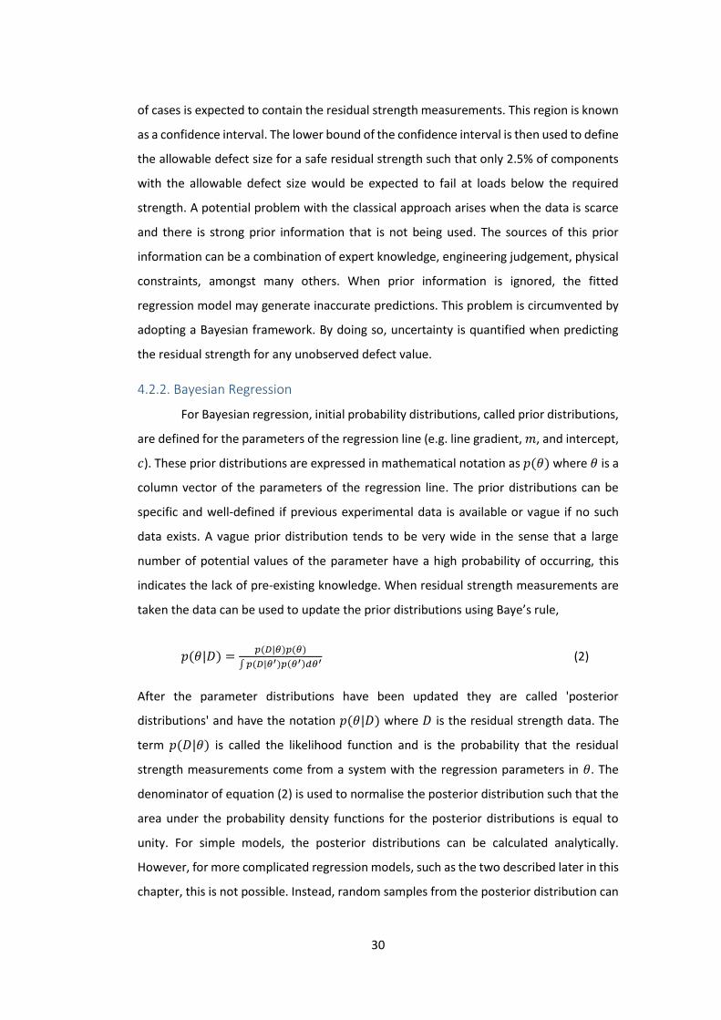
30

of cases is expected to contain the residual strength measurements. This region is known

as a confidence interval. The lower bound of the confidence interval is then used to define

the allowable defect size for a safe residual strength such that only 2.5% of components

with the allowable defect size would be expected to fail at loads below the required

strength. A potential problem with the classical approach arises when the data is scarce

and there is strong prior information that is not being used. The sources of this prior

information can be a combination of expert knowledge, engineering judgement, physical

constraints, amongst many others. When prior information is ignored, the fitted

regression model may generate inaccurate predictions. This problem is circumvented by

adopting a Bayesian framework. By doing so, uncertainty is quantified when predicting

the residual strength for any unobserved defect value.

4.2.2. Bayesian Regression

For Bayesian regression, initial probability distributions, called prior distributions,

are defined for the parameters of the regression line (e.g. line gradient, 𝑚, and intercept,

𝑐). These prior distributions are expressed in mathematical notation as 𝑝(𝜃) where 𝜃 is a

column vector of the parameters of the regression line. The prior distributions can be

specific and well-defined if previous experimental data is available or vague if no such

data exists. A vague prior distribution tends to be very wide in the sense that a large

number of potential values of the parameter have a high probability of occurring, this

indicates the lack of pre-existing knowledge. When residual strength measurements are

taken the data can be used to update the prior distributions using Baye’s rule,

2

𝑝(𝜃|𝐷) =𝑝(𝐷|𝜃)𝑝(𝜃)

∫ 𝑝(𝐷|𝜃′)𝑝(𝜃′)𝑑𝜃′ (2)

After the parameter distributions have been updated they are called 'posterior

distributions' and have the notation 𝑝(𝜃|𝐷) where 𝐷 is the residual strength data. The

term 𝑝(𝐷|𝜃) is called the likelihood function and is the probability that the residual

strength measurements come from a system with the regression parameters in 𝜃. The

denominator of equation (2) is used to normalise the posterior distribution such that the

area under the probability density functions for the posterior distributions is equal to

unity. For simple models, the posterior distributions can be calculated analytically.

However, for more complicated regression models, such as the two described later in this

chapter, this is not possible. Instead, random samples from the posterior distribution can

31

be generated using Markov Chain Monte Carlo (MCMC) techniques. For this thesis, the

MCMC algorithm known as Gibbs sampling, described extensively in [24], has been used

to generate a large number of samples of the possible parameter values for the regression

model. The histogram of these random samples will have the same shape as the posterior

distribution for each parameter, an example for samples from a normal distribution is

shown in Figure 6. This means percentiles of the random samples will be very close to the

percentiles of the underlying probability distribution. Thus, if the random samples are

potential values of residual strength, then the percentiles can be used to make

conservative residual strength predictions.

Figure 6: Histogram of 5000 samples randomly distributed with a normal distribution (with 𝜇 = 0 and 𝜎 = 1),

with the probability distribution function of the normal distribution, 𝑝(𝑦), superimposed.

4.3. Experimental Method

Two sets of composite specimens, with in-plane dimensions of 250 mm by 90 mm,

were manufactured using two different material systems and layups. Since laminates

consisting of unidirectional plies are particularly sensitive to impacts [6], unidirectional

prepregs were used to manufacture the specimens for this experiment. Twelve crossply

carbon fibre laminates were produced from M10R-UD-150 unidirectional prepreg (Hexcel,

32

USA) with a [02/902/02/902/02/90]S layup, where the 0° plies were parallel to the longest

edge. The prepreg laminate was cured in a hot press (APV-3530, Meyer, Germany) at a

temperature of 130 °C and a pressure of 2.5 bar for 45 minutes as per the manufacturer’s

recommendations. The press was heated up to temperature at a rate of 10 °C/min and

after curing was left to cool naturally with the pressure maintained. A second batch of

specimens with a different layup was produced to demonstrate the rigour of the defect

assessment. The different layup affects the size and shape of impact damage in the

laminate [6]. Twenty-five quasi-isotropic carbon fibre laminates were produced from

RP507UT210 prepreg (PRF, UK) with a [02/902/452/-452]S layup using an identical process.

The nominal thickness of the crossply and quasi-isotropic specimens were 2.90 mm and

3.02 mm respectively.

A drop weight impactor, identical to the one employed by Yang and Cantwell [7],

was used to produce barely visible impact damage in the laminates with a 20 mm

diameter hemispherical tup of mass 2.67 kg. The specimens were clamped onto a metal

support with a 125 mm by 75 mm opening underneath them. The eleven crossply

specimens were impacted with a range of energies between 4 and 14 J leaving a single

virgin specimen. Eighteen quasi-isotropic specimens were impacted with a range of

energies between 4 and 15 J, leaving seven virgin specimens.

The specimens were then cut down to 220 mm by 40 mm coupons using a wet

diamond saw (Versatile 103450, Vitrex, USA). The use of the wet diamond saw resulted in

clean edges on the specimens and did not produce edge delaminations. The impact

location was used as the centre of the specimens.

After each impact, the delaminations in the composite were evaluated using

pulse-echo ultrasound. A time-of-flight C-scan was captured using the equipment and

technique described in Chapter 3. The width, length and area of the defects were

evaluated from the C-scans. After the defect evaluation using ultrasound, the coupons

were loaded to failure using a servo-hydraulic load frame (8501, Instron, USA) in a four-

point bend setup with a support span of 160 mm and load span of 80 mm. Each coupon

was placed in the loading rig such that the impact damage was centred in the load span

and the impacted surface was in tension. The specimens were loaded under displacement

control at a rate of 0.8 mm/min and failure was defined as the point at which the force

33

dropped below 50% of its peak value. The maximum bending moment was recorded and

used as the measure of the residual strength of the coupon.

The ultrasound defect, 𝑥𝑖, and residual strength, 𝑦𝑖, measurements were

normalised using:

3

𝑥𝑖∗ =

𝑥𝑖−�̅�

𝑠𝑥 (3)

4

𝑦𝑖∗ =

𝑦𝑖−�̅�

𝑠𝑦 (4)

where �̅� and �̅� are the mean of the ultrasound measurements of defect size and residual

strength measurements respectively, and 𝑠𝑥 and 𝑠𝑦 are their standard deviations. The

normalisation allowed the use of the same prior distributions for Bayesian regression

regardless of the units used in the ultrasound and residual strength measurements. The

normalisation also increased the efficiency of the Gibbs sampler, by reducing the number

of iterations required to represent the predictive distribution, because it ensured that the

potential values for the gradient and intercept were close to zero and of approximately

the same scale, so that large perturbations were not introduced during sampling.

4.4. Bayesian Modelling

4.4.1. Robust Bayesian Linear Regression

The model used to predict residual strength based on ultrasound measurements

was linear, of the form 𝑦∗ = 𝑚𝑥∗ + 𝑐, with the assumption that the data was distributed

around the regression line as a Student’s t-distribution. This distribution was employed

because it allowed the deviation of residual strength measurements from the regression

line to have a greater probability of outliers, compared to the normal distribution. Thus,

when present, outliers were expected to have less effect on the intercept and gradient of

the regression line. The form of the model is shown schematically in the bottom portion

of Figure 7, in a similar style as the one employed in [24]. The shape of the distribution

about the line shown in the centre portion is a t-distribution defined by its normality, 𝑣𝑠,

spread, 𝜎𝑠, and mean, 𝜇𝑠, which in turn is defined by the gradient of the line, 𝑚𝑠, and its

intercept, 𝑐𝑠. Each of these four parameters: normality, spread, gradient and intercept are

described by prior distributions that are shown schematically in the top portion of Figure

7. It was decided to represent the prior distribution for the normality parameter by an

34

exponential distribution in order to allow it to vary from low values that causes the t-

distribution to have long tails, to high values at which the t-distribution behaved like a

normal distribution. The probability density function, 𝑝(𝑦∗), for the t-distribution

illustrating this behaviour is shown in Figure 8. The exponential distribution has a scale

parameter, 𝐾, of 29. The prior distributions of the gradient and intercept of the line-of-

best-fit have been defined as normal distributions, which is the common choice for simple

regression models [85]. In both normal distributions the means, 𝑀𝑐 and 𝑀𝑚, were set to

zero as the normalisation process in equations (3) and (4) cause the values of both the

intercept and gradient to be close to zero. The standard deviations, 𝑆𝑐 and 𝑆𝑚, of the

normal distributions are also defined with a high value of 100, which ensures that the

prior distributions are vague and thus will not limit the potential values of the gradient

and intercept. The probability distribution describing the prior distribution of the spread

of the t-distribution, 𝜎𝑠, was a uniform distribution that assigned an equal probability to

values of the spread from 𝐿 = 1 × 10−3 to 𝐻 = 1 × 103. All of the parameters used to

define the initial or prior probability distributions are listed in Table 1.

35

Figure 7: Schematic diagram showing how the regression model (bottom) is formed from a linear regression

line with the data distributed around it in the form of a t-distribution (middle). At the top are the initial or prior

probability distributions for the values of the model parameters.

36

Figure 8: Illustration of the probability density function for the t-distribution as a function of the normality

parameter ν for a mean, 𝜇 = 0 and spread, 𝜎 = 1. As ν tends to infinity, the t-distribution converges to a

normal distribution.

Table 1: The values used to define the vague prior probability distributions for the regression model

parameters, these values are suggested in [24].

Parameter Prior Value

𝐾 29

𝑀𝑐 0

𝑆𝑐 100

𝑀𝑚 0

𝑆𝑚 100

𝐿 1 × 10−3

𝐻 1 × 103

The regression model was fitted to the residual strength data using the open-

source software JAGS [25] to determine the posterior distributions of the parameters,

that is the normality, 𝜈 and spread, 𝜎 of the t-distribution together with the gradient, 𝑚

and intercept, 𝑐 of the regression line. Subsequently, these posterior parameters can be

used to predict the residual strength of a defective composite structure when a particular

size of impact damage has been identified. Since the posterior parameters are each

37

represented by a probability distribution, the prediction also results in a probability

distribution that is called the posterior predictive distribution. This predictive distribution

can be computed using a random number generator such that when 𝜈(𝑗), 𝑚(𝑗), 𝑐(𝑗) and

𝜎(𝑗) are the 𝑗th samples from the posterior distributions, then the 𝑗th sample of the

predicted strength is given by

5

𝑦(𝑗) = 𝑡𝑟𝑛𝑑 (𝑚(𝑗) (𝑥−�̅�

𝑠𝑥) + 𝑐(𝑗), 𝜎(𝑗), 𝜈(𝑗)) × 𝑠𝑦 + �̅� (5)

where 𝑡𝑟𝑛𝑑( ) is a generator of random numbers conforming to a t-distribution and, as in

equations (3) and (4), �̅� and �̅� are the mean of the ultrasound defect and residual strength

measurements respectively, and 𝑠𝑥 and 𝑠𝑦 are their corresponding standard deviations.

The JAGS software package was used to generate 500,000 random samples at each 𝑥

location and ranked by the magnitude of the predictive residual strength in order to allow

the 2.5th, 50th and 97.5th percentiles to be identified. A typical result is shown in Figure 9

with an interval defined using the 2.5th and 97.5th percentiles from the predictive

distribution. The 50th percentile of 𝑦 was used to plot the line-of-best-fit. The locations at

which the percentiles were calculated are marked with dots. The code for performing

robust Bayesian linear regression is included in this thesis as Appendix A and Appendix B.

It is important to note that when using percentiles of the predictive distribution, the

interval generated is commonly called a credible interval. The distinction between the

classical confidence intervals and the Bayesian credible interval is subtle but important.

In the classical (frequentist) view, parameters are fixed but unknown. Thus, a 95%

confidence interval is expected to include the true value of the parameter 95% of the time

in repeated sampling. The interval, not the true value of the unknown parameter, is

random. From the Bayesian point of view, the value of the parameter is considered

random and a 95% credible interval is expected to contain 95% of the probability

distribution of the parameter. Under certain conditions, confidence and credible intervals

may coincide. For a detailed account on the similarities and differences in methodology

and philosophy of construction refer to [86].

38

Figure 9: A typical predictive distribution of residual strength, y*, as a function of ultrasound measurement,

x*, based on a Bayesian linear regression model fitted to the measured data values (crosses) with prediction

uncertainties and a 95% credible interval. The dots on the three lines indicate the locations at which percentiles

of the predictive distribution were calculated. The lines are spline curves interpolated through the quantified

points.

4.4.2. Piecewise Robust Bayesian Regression

To perform piecewise robust Bayesian regression, the only part of the model

described in the previous section that must be changed is how the mean of the t-

distribution, 𝜇𝑠, is obtained. Instead of the t-distribution mean being calculated using a

simple linear function, it is instead calculated using a discontinuous basis function, shown

schematically at the bottom of Figure 10. This basis function has a discontinuity at a

transition point, 𝜉𝑠, where the value of the t-distribution mean changes from a constant,

to a linear function. The transition parameter was given a uniform prior distribution with

the upper and lower bounds of the distribution set to the maximum and minimum values

of 𝑥∗ respectively. This prior distribution allows the transition to occur at any value of

defect severity. The linear function in the second half of the basis function is defined with

two parameters: gradient, 𝑚𝑠, and intercept, 𝑐𝑠. These parameters have normal prior

distributions where the means and standard deviations of the prior distributions were set

to the same values used for the linear function in the robust Bayesian linear regression

model, these values are listed in Table 1. The regression model was fitted to the residual

strength data using the open-source software JAGS [25] to determine the posterior

distributions of the parameters. To generate samples of the posterior predictive

39

distribution of the piecewise Bayesian regression model, equation (5) can be modified to

include the samples of the transition parameter 𝜉(𝑗) as such:

6

𝑦(𝑗) = {𝑡𝑟𝑛𝑑(𝑚(𝑗)𝜉(𝑗) + 𝑐(𝑗), 𝜎(𝑗), 𝜈(𝑗)) × 𝑠𝑦 + �̅� , (

𝑥−�̅�

𝑠𝑥) ≤ 𝜉(𝑗)

𝑡𝑟𝑛𝑑 (𝑚(𝑗) (𝑥−�̅�

𝑠𝑥) + 𝑐(𝑗), 𝜎(𝑗), 𝜈(𝑗)) × 𝑠𝑦 + �̅� , (

𝑥−�̅�

𝑠𝑥) > 𝜉(𝑗)

(6)

After samples of the posterior predictive distribution were obtained, it was then possible

to calculate the bounds of the credible interval. This was performed in the same way as

for robust Bayesian linear regression using percentiles of the posterior predictive

distributions. It is also possible to reverse the behaviour of the basis function such that

the linear interval is first which transitions into a constant-valued interval. The code for

performing piecewise robust Bayesian regression is included in this thesis as Appendix A

and Appendix C.

Figure 10: Schematic diagram showing how the basis function for piecewise robust Bayesian regression (solid

black line in the bottom graph) is formed using three parameters and the prior distributions for those

parameters (top).

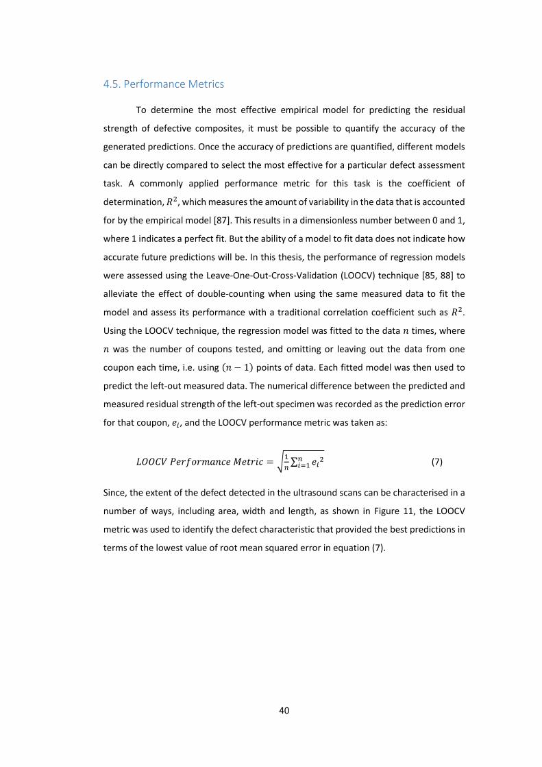
40

4.5. Performance Metrics

To determine the most effective empirical model for predicting the residual

strength of defective composites, it must be possible to quantify the accuracy of the

generated predictions. Once the accuracy of predictions are quantified, different models

can be directly compared to select the most effective for a particular defect assessment

task. A commonly applied performance metric for this task is the coefficient of

determination, 𝑅2, which measures the amount of variability in the data that is accounted

for by the empirical model [87]. This results in a dimensionless number between 0 and 1,

where 1 indicates a perfect fit. But the ability of a model to fit data does not indicate how

accurate future predictions will be. In this thesis, the performance of regression models

were assessed using the Leave-One-Out-Cross-Validation (LOOCV) technique [85, 88] to

alleviate the effect of double-counting when using the same measured data to fit the

model and assess its performance with a traditional correlation coefficient such as 𝑅2.

Using the LOOCV technique, the regression model was fitted to the data 𝑛 times, where

𝑛 was the number of coupons tested, and omitting or leaving out the data from one

coupon each time, i.e. using (𝑛 − 1) points of data. Each fitted model was then used to

predict the left-out measured data. The numerical difference between the predicted and

measured residual strength of the left-out specimen was recorded as the prediction error

for that coupon, 𝑒𝑖, and the LOOCV performance metric was taken as:

7

𝐿𝑂𝑂𝐶𝑉 𝑃𝑒𝑟𝑓𝑜𝑟𝑚𝑎𝑛𝑐𝑒 𝑀𝑒𝑡𝑟𝑖𝑐 = √1

𝑛∑ 𝑒𝑖

2𝑛𝑖=1 (7)

Since, the extent of the defect detected in the ultrasound scans can be characterised in a

number of ways, including area, width and length, as shown in Figure 11, the LOOCV

metric was used to identify the defect characteristic that provided the best predictions in

terms of the lowest value of root mean squared error in equation (7).

41

Figure 11: A typical time-of-flight C-scan of impact damage in a quasi-isotropic composite laminate, showing

the defect metrics used. The defect area was defined as the projected area of all the delaminations when

viewed in the C-scan. Colour is used to indicate the depth of delaminations from the impacted surface.

4.6. Results

A typical time-of-flight ultrasound C-scan from an impacted coupon is shown in

Figure 11. The area, width and length of the defect were used as defect metrics and their

efficacy for predicting residual strength compared, as described in the previous section.

The width was defined as the total width of the delaminations perpendicular to the

loading direction when viewed from above, as defined by Prichard and Hogg [12]. Defect

length was measured similarly, but parallel to the loading direction. The defect area was

taken as the total projected area of the delaminations when viewed from the impacted

face using time-of-flight ultrasound. As the impact energy was increased, the size of the

delaminations caused by the impact increased as well. This can be seen for both quasi-

isotropic coupons and crossply coupons in Figure 12 and Figure 13 respectively.

42

Figure 12: Time-of-flight C-scans of quasi-isotropic coupons with increasing impact energies of 5J, 8J, 12J and

15J.

Figure 13: Time-of-flight C-scans of crossply coupons with increasing impact energies of 5J, 8J, 10J and 12J.

Figure 14 shows the Bayesian linear regression predictions of the residual

strength of quasi-isotropic coupons using area, length and width of the ultrasound data

(as shown in Figure 11) as the defect metric. Similar plots for predicting the residual

strength of crossply coupons are shown in Figure 15. The LOOCV performance metric was

used to assess the accuracy of predictions made using the different measurements. The

lowest value indicates the measurement that is expected to result in the most accurate

predictions. The LOOCV performance metrics, listed in Table 2, reveal that the area of the

defect is the best metric for predicting the residual strength for both the quasi-isotropic

and crossply coupons.

43

Figure 14: Residual strength predictions made using Bayesian linear regression for impacted quasi-isotropic

specimens using ultrasound measurements of defect area (top), length (middle) and width (bottom) as the

defect metric. The size of the 95% credible interval (grey shading) indicates that the uncertainty is smallest

when the area of the defect was used as the defect metric which concurs with the LOOCV performance metric

data in Table 2.

44

Figure 15: Residual strength predictions made using Bayesian linear regression for impacted crossply coupons

using ultrasound measurements of defect area (top), length (middle) and width (bottom) as the defect metric.

45

Table 2: LOOCV performance metrics indicating the average uncertainties of residual strength predictions for

crossply and quasi-isotropic specimens using three different defect metrics to make predictions. The 𝑅2

statistics for the same regression models are also shown.

Defect Metric

Bayesian Regression Classical Regression

Crossply Quasi-isotropic Crossply Quasi-isotropic

LOOCV

(Nm)

𝑹𝟐

(-)

LOOCV

(Nm)

𝑹𝟐

(-)

LOOCV

(Nm)

𝑹𝟐

(-)

LOOCV

(Nm)

𝑹𝟐

(-)

Defect Area 2.517 0.830 5.325 0.763 2.500 0.830 5.341 0.763

Defect Length 3.388 0.697 6.230 0.678 3.385 0.697 6.232 0.678

Defect Width 3.290 0.705 6.923 0.603 3.288 0.705 6.923 0.603

The predictions from Bayesian linear regression form a straight line as expected

while the corresponding uncertainties are a pair of curves above and below the regression

line defining a credible interval such that 95% of results for all coupons evaluated with

ultrasound (to provide a value of the defect metric, 𝑥∗) and then tested to failure (to

provide a value of residual strength, 𝑦∗) would be expected to lie in. Residual strength

predictions were made for a range of defect metric values from zero, indicating no defect

found, to the point at which the defect causes the residual strength to be approximately

half the virgin strength. An example of how the plots in Figure 14 and Figure 15 can be

used for making conservative estimates of residual strength is shown in Figure 16.

46

Figure 16: Residual strength predictions made using Bayesian linear regression for impacted crossply

specimens using the defect area from the ultrasound measurements as the defect metric together with the

95% credible interval (grey shading). The dotted lines indicate an exemplar minimum residual bending strength

and the corresponding maximum allowable defect area for coupons with a probability of failure of less than

2.5%.

4.7. Discussion

The graphs in Figure 14 and Figure 15 show the predictions of the residual

strength as a function of the size of defect and are directly comparable to the ones

produced by Prichard and Hogg [12] with the same correlation between defect width and

residual strength demonstrated. There is substantial scatter above and below the

regression line in the measured residual strengths, which is likely due to the complex

nature of impact damage involving both fibre breakage and matrix cracking within the

area of impact damage [6]. It is not possible to resolve these microscale features using

ultrasound and a much more sophisticated model would be required to incorporate such

detail into the residual strength predictions (e.g. [54] where an FE model was developed

that predicted the propagation of delaminations produced by impact damage). However,

the Bayesian approach employed here together with the use of the calculated credible

interval allows all of the potential sources of uncertainty, including both the noise in the

ultrasound measurements and the behaviour of the unmeasured microscale damage, to

be accounted for in the predictions. The lower bound of the credible interval can be used

to specify the maximum allowable size of a defect for a specified minimum residual

strength. For instance, if the minimum tolerable residual bending strength for the crossply

coupons is 32 Nm, then the maximum allowable area of a defect detected by ultrasound

47

would be 341 mm2, as shown by the dotted lines in Figure 16. This would ensure that

coupons with a probability of 2.5% or more of failing at loads below the minimum residual

strength are taken out of service for repair or disposal.

The LOOCV performance metric, values given in Table 2, was used to demonstrate

that defect area was the best choice for residual strength predictions for both the crossply

and quasi-isotropic specimens, as predictions were up to 25% more accurate than when

using the other defect metrics. The 𝑅2 statistics, also shown in Table 2, also demonstrate

that defect area is the best empirical model, however this statistic does not estimate the

average uncertainty of future predictions. The use of the best available defect metric for

residual strength predictions reduces the size of the credible intervals, as can be seen in

Figure 14, which raises the maximum allowable size of a defect permitted for the same

probability of failure for a given required residual strength. This is likely to reduce the

number of components that are removed unnecessarily from service for repair or disposal

and hence reduce operating costs. Table 2 contains LOOCV performance metrics for both

Bayesian and classical regression models showing that for data that does not contain

outliers, the two regression techniques have similar behaviour.

The relative performance of the classical and Bayesian linear regression models

were compared for a small dataset by using a subset of data from just four of the crossply

coupons. The two techniques produce the same regression line but substantially different

intervals as shown in Figure 17. When calculating the allowable defect size for a coupon

with a residual strength of 32 Nm the classical regression model over predicted the

allowable defect size by almost 40%. In contrast, as the data set was small, the uncertainty

on the Bayesian regression predictions were high and thus a conservative allowable defect

size was determined that was 32% smaller than when the defect size was calculated using

the full dataset. This implies that classical regression tends to underestimate the

prediction uncertainty in the presence of limited or small datasets while the Bayesian

analysis is conservative. This occurs because the normalisation, described in equations (3)

and (4), ensures that the spread, s of the measured residual strengths around the

regression line are always towards the lower end of the corresponding prior distribution,

shown in Figure 7 and Table 1, and thus as more coupons are tested the credible interval

will collapse towards the measurements. These conservative estimates of the allowable

defect size ensure that unexpected failures are unlikely.

48

Figure 17: Residual strength predictions made using Bayesian linear regression for a small set of four impacted

quasi-isotropic specimens. Strength predictions were based on ultrasound measurements of defect area. The

wide light grey region is the Bayesian regression credible interval and the narrow dark grey region is the

classical regression confidence interval.

The influence of outliers on Bayesian regression can be explored using an artificial

set of data generated using the following linear function:

8

𝑦𝑖 = −3𝑥𝑖 + 60 + 𝑁𝑟𝑛𝑑(0, 0.32) (8)

where 𝑥𝑖 = {3,4,5, ⋯ ,12} and 𝑁𝑟𝑛𝑑(0, 0.32) is a random number generator that

produces numbers with a normal-distribution of mean value of 0 and standard deviation

of 0.3. The classical and Bayesian linear regressions and the corresponding intervals

calculated from this data were identical, as expected, and thus only the Bayesian linear

regression is shown in Figure 18. However, when an outlier was introduced by changing a

single value, 𝑦2 = 30, the behaviour of the two techniques was substantially different, as

shown in Figure 19. The gradient and intercept of the Bayesian regression is unchanged

with the line-of-best-fit equation being almost identical to the linear function in equation

(8). For classical linear regression, the gradient has increased to -2.2, an error of 26% of

the value used in equation (8) to generate the data. The credible intervals are larger in

the presence of the outlier by a factor of 3.3 and 12.2 respectively for the Bayesian and

classical regression models. This suggests that the Bayesian regression model is more

robust in the presence of outliers, which is expected, because in these circumstances

Gibbs sampling will assign higher probabilities to low values of the normality parameter

of the t-distribution so that outliers have little effect on the slope and gradient

49

distributions for the regression line. Consequently, when using the Bayesian model, there

is no need to identify and remove outliers from measured data as is common practice

when using other regression techniques [22, 23]. The LOOCV performance metric and 𝑅2

were calculated for both regression models when an outlier was present and are shown

in Table 3. When choosing the best performing regression model, the 𝑅2 statistic

incorrectly identified the classical regression model as having marginally higher

performance despite the regression line not following the data trend. The LOOCV

performance metric is 13% lower for the Bayesian regression model and thus correctly

identified the Bayesian regression model as the best choice for future predictions. This is

because the LOOCV performance metric actually tests the regression models ability to

predict new data whilst 𝑅2 only indicates how well the regression line fits the available

data.

Figure 18: Bayesian linear regression based on artificial data generated using the linear function in equation

(8) with normally distributed measurement noise.

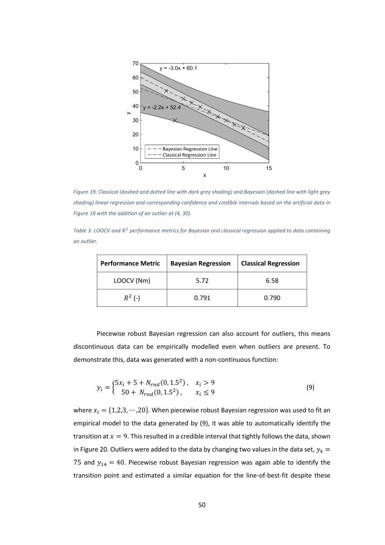
50

Figure 19: Classical (dashed and dotted line with dark grey shading) and Bayesian (dashed line with light grey

shading) linear regression and corresponding confidence and credible intervals based on the artificial data in

Figure 18 with the addition of an outlier at (4, 30).

Table 3: LOOCV and 𝑅2 performance metrics for Bayesian and classical regression applied to data containing

an outlier.

Performance Metric Bayesian Regression Classical Regression

LOOCV (Nm) 5.72 6.58

𝑅2 (-) 0.791 0.790

Piecewise robust Bayesian regression can also account for outliers, this means

discontinuous data can be empirically modelled even when outliers are present. To

demonstrate this, data was generated with a non-continuous function:

9

𝑦𝑖 = {5𝑥𝑖 + 5 + 𝑁𝑟𝑛𝑑(0, 1.52) , 𝑥𝑖 > 9

50 + 𝑁𝑟𝑛𝑑(0, 1.52) , 𝑥𝑖 ≤ 9 (9)

where 𝑥𝑖 = {1,2,3, ⋯ ,20}. When piecewise robust Bayesian regression was used to fit an

empirical model to the data generated by (9), it was able to automatically identify the

transition at 𝑥 = 9. This resulted in a credible interval that tightly follows the data, shown

in Figure 20. Outliers were added to the data by changing two values in the data set, 𝑦4 =

75 and 𝑦14 = 40. Piecewise robust Bayesian regression was again able to identify the

transition point and estimated a similar equation for the line-of-best-fit despite these

51

outliers, as shown in Figure 21. The width of the credible interval increased but this is to

be expected. With the addition of two outliers, the data suggests there is a significant

probability of future measurements being outliers and thus the credible interval must be

wider to indicate the potential for these outliers to occur. If the same task was to be

performed using classical regression, prior knowledge of the location of the transition

point or categorisation of the data into one interval or the other would introduce too

many subjective judgements regarding the data. To perform this task with classical

regression would also require the removal of the outliers resulting in a credible interval

that is too narrow.

Figure 20: Piecewise robust Bayesian regression applied to non-continuous data generated using equation (9).

Figure 21: Piecewise robust Bayesian regression applied to non-continuous data generated using equation (9)

with two outliers.

52

The Gibbs sampling algorithm used to perform Bayesian regression took on

average 33 s to fit the regression model using a PC with an Intel Core i7-960 processor.

The classical regression was performed using the same data in approximately 0.02 s on

the same computer. The disparity in computational speed is due to classical linear

regression using analytical equations whilst Bayesian linear regression uses iterative Gibbs

sampling. However, the application of the Bayesian regression model is simpler than a

computational mechanics model and allows defect prognoses to be made quickly whilst

incorporating all of the uncertainties. Bayesian regression also allows regression to be

applied to nonlinear data with minimal input by the user. In this chapter, measurements

taken from ultrasound C-scans were correlated with residual bending strength but the

approach is generic and any measurement from a non-destructive evaluation technique

could be correlated to an important performance metric. In later chapters the two

introduced Bayesian regression techniques were applied to different non-destructive

measurements and for predicting different quantities without any modification to the

statistical techniques.

4.8. Conclusion

Bayesian linear regression has been used to create a model of the residual

strength in bending after impact of carbon fibre composite coupons, based on ultrasound

measurements in both crossply and quasi-isotropic laminates. The performance of the

model was found to be more robust than classical linear regression. In more detail, C-scan

data was generated for twenty-five quasi-isotropic coupons and twelve crossply coupons

that had been subject to drop-weight impacts in the range 0 to 15 J using a 20 mm

diameter tup. The coupons were tested to failure in four-point bending in order to

determine their residual strength. A Bayesian linear regression model was fitted to the

measured ultrasound and strength data using Gibbs sampling and the performance of the

model evaluated using the LOOCV performance metric.

The empirical model based on defect area, measured using ultrasonic C-scans,

was found to yield smaller prediction uncertainties than using either the defect length or

width. The LOOCV performance metric was used to estimate the average uncertainty of

future predictions and found that for both the crossply and quasi-isotropic specimens

using defect area results in prediction uncertainties that are approximately 25% smaller

than using either defect length or defect width.

53

It was found that a classical linear regression model tended to underestimate the

uncertainty in predictions of residual strength and thus overestimate the allowable defect

size when only a limited amount of experimental measurements was available. In the

example given in this chapter, this overestimation was 40%. In these circumstances, the

Bayesian linear regression model provided conservative estimates of the prediction

uncertainty, thus underestimating the allowable defect size. This implies that the use of

the Bayesian model might lead to the rejection of some serviceable components but it is

unlikely to compromise safety. An additional advantage of the Bayesian approach is that

the model can be updated as more experimental data becomes available. In the presence

of outliers in the measured data, Bayesian regression was shown to provide accurate

estimations of prediction uncertainties whereas classical linear regression provided very

conservative estimations, with a 95% confidence interval that was almost four times

larger than the interval calculated using Bayesian regression. Bayesian regression was still

able to accurately estimate the parameters of the function used to generate the data

containing outliers whilst classical regression estimates of gradient were different by 26%.

The 𝑅2 statistic in the presence of data outliers wrongly identified the classical regression

model as being more adequate, unlike LOOCV. A second type of Bayesian regression was

also introduced, allowing for empirical models to be generated for non-continuous data

whilst still being robust to outliers. It is not possible to perform this task with classical

regression without subjective judgements and discarding data.

Normalisation of the measured data was used to provide a generic approach to

implementing the Bayesian regression model using Gibbs sampling. However, the main

drawback of both the Bayesian regression model and the LOOCV performance metric is

the high computation time required for the calculations. Once the calculations have been

completed the defect assessments can be performed rapidly using residual strength

predictions based on non-destructive evaluation, without the need for expert

interpretation or analysis. It is proposed that the Bayesian model has the potential to

permit improved decision-making on the serviceability of defective composite

components as a result of more robust and reliable predictions of residual behaviour and

accurate estimates of the uncertainty in the predictions. This is likely to reduce

unnecessary repairs and replacements and thus decrease maintenance costs and down-

time.

54

5. Strain-based Defect Assessment of Impacted Composite

Laminates

5.1. Introduction

There are substantial costs associated with the repair of composite structures,

hence it would be beneficial for the assessment techniques to provide the most suitable

information for characterising the defect. This could help to reduce the number of repairs

to those that are essential for the structure to be safely operated. Ultrasound and

thermography are amongst the most common techniques currently employed to assess

aerospace composites [3], and provide information in the form of the size and shape of

the defect. From this data, the residual strength of the structure can be inferred, but

predictions based on these measurements have high levels of uncertainty because the

effect of the defect on the structural integrity is not completely characterised [4]. The

changes in strain fields induced by the defect should provide the most appropriate input

parameters for predicting the change in structural integrity, or residual strength [2]. Thus,

employing strain fields to assess the effect of defects in composites is likely to lead to

more reliable predictions of the residual strength.

To determine how much of an improvement can be obtained by using a strain-

based assessment compared to an ultrasound assessment, the statistical techniques

introduced in the previous chapter are applied to a strain-based defect assessment

described in this chapter. The experiments detailed in this chapter extend the defect-

assessment technique developed by Patki and Patterson [5] to predicting the residual

strength of impacted coupons. The strain-based defect assessments described here were

performed in parallel to ultrasound-based inspections and as such direct comparisons can

be made between the two assessment techniques.

This chapter is based on the following published paper, written by the author of

this thesis:

Christian WJR, DiazDelaO FA, Patterson EA. “Strain-based Damage Assessment for

Accurate Residual Strength Prediction of Impacted Composite Laminates”. Composite

Structures. 2017.

55


Two different material systems and layups were chosen to explore the accuracy

of strain-based residual strength predictions. Eight crossply coupons were produced using

M10R-UD-150 prepreg (Hexcel, USA) with a [02/902/02/902/02/90]S layup. Nineteen quasi-

isotropic coupons with a [02/902/452/-452]S layup were manufactured using RP507UT210

prepreg (PRF, UK) and cured with an identical method to that used for the coupons

described in Chapter 4.

Barely visible impact damage (BVID) was created in the laminates using a drop-

weight impact tower. A 20 mm hemispherical tup of mass 2.67 kg was used to produce

damage without forming cracks on the impacted surface of the coupon. The only damage

visible was a shallow dimple with a typical diameter of 5 mm on the impacted surface.

Seven of the crossply laminates were impacted with a range of energies between 4 J and

12 J, leaving a single virgin laminate. Thirteen of the quasi-isotropic laminates were

impacted at a range of energies between 4 J and 15 J, leaving six virgin laminates. The

laminates were then cut into 220 mm by 40 mm coupons using a wet diamond saw

(Versatile 103450, Vitrex, USA) with the impact location used as the centre of the coupons

and the 0⁰ plies running in the x-direction, as shown in Figure 22. A wet diamond saw was

used to ensure the cut edges were free from delaminations that may have caused

premature failure.

Figure 22: A coupon with speckle pattern applied at the location where the impact was applied showing

dimensions and the coordinate system used for the DIC and ultrasound measurements.

The spatial distribution of the delaminations produced by the impacts were

measured using pulse-echo ultrasound. The process used to produce time-of-flight C-

scans is explained in Chapter 3. Time-of-flight C-scans are images that show the position

and depth of defects within a laminate. After the ultrasonic inspection, the strain-based

defect assessment, explained in the next section, was performed. Since the strain-based

56

defect assessment required a load to be applied to each coupon, a further ultrasonic

inspection was performed after the strain-based assessment was complete to check that

the delaminations had not propagated. The delaminations in one quasi-isotropic coupon,

which was impacted with an energy of 15 J, had propagated and hence, data for this

coupon was not included in any further analysis.

After the final ultrasound inspection, each coupon was loaded to failure using a

four-point bend setup. A servo-hydraulic load frame (8501, Instron, USA) with a four-point

bending rig, consisting of a support span and load span of 160 mm and 80 mm

respectively, was used to load the coupons. The coupons were placed in the bending rig

such that the impacted surface was in tension; and thus, the large delaminations close to

the rear surface, were in compression. The load frame was then operated under

displacement control to monotonically load the coupons to failure at a rate of

0.8 mm/min. The coupons were considered to have failed when their stiffness was

reduced to 50% of its original value. The ultimate bending moments were recorded and

used as the residual strength for the coupons. The measurement of residual strength in

bending was chosen because the loads required for failure in tension or compression were

expected to exceed ±100 kN and thus were too high for the load frame.

5.3. Strain-Based Defect Assessment

To perform DIC, a speckle pattern was first applied to a 50 mm wide area in the

middle of each coupon on the surface that was impacted, a photograph of a speckled

coupon is shown in Figure 22. The DIC setup used for this experiment is described in

Chapter 3 and a photo of an impacted coupon during loading is shown in Figure 23. The

impacted surface was chosen for the strain-based inspection because aerospace

structures are typically inspected on the most accessible surface, which is also likely to be

the surface that experiences impacts.

57

Figure 23: Coupon under four-point bend load with the cameras used for DIC attached to the top half of the

rig facing the impacted surface of the coupon.

Each coupon was loaded to the same displacement by vertically moving the

loading span 6 mm towards the support span, where a displacement of 0 mm would

indicate all four noses of the four-point bend rig were in contact but not inducing a

bending moment in the coupon. The application of a common displacement instead of

bending moment ensured that variations in the stiffness of the virgin material does not

affect the defect assessment; and, that only variations in redistribution of the strain due

to the defect are measured [35]. Each coupon was loaded 6 times and the strain field

captured each time. The common displacement resulted in a mean bending moment

applied to the crossply and quasi-isotropic coupons of 20.36 Nm and 21.38 Nm

respectively.

58

The strain fields contained large quantities of data, much of it redundant, and

thus the dimensionality of the fields were reduced prior to performing the defect

assessment. Once each strain field was captured, a 25 mm wide square area of the strain

field was selected with the centre defined by the surface dimple caused by the impactor.

The width of this square area was chosen to be approximately the same as the y-direction

width of the largest defect detected using ultrasound. If the area of strain data used for

assessments was substantially larger than the defect, only a small portion of the strain-

field would be affected by the defect, limiting the sensitivity of the technique. The square

area of strain data was dimensionally reduced using the technique of image

decomposition [50]. Image decomposition is the process by which an image consisting of

a large number of pixels can be represented by a comparatively small number of shape

descriptors. Orthonormal discrete Tchebichef polynomials [47] were used to describe

each strain field and hence, to provide these shape descriptors. The Tchebichef shape

descriptors for an N x N discrete image, 𝐼(𝑖, 𝑗), are given as [47]:

10

𝑇𝑝,𝑞 =1

�̃�(𝑝,𝑁)�̃�(𝑞,𝑁)∑ ∑ �̃�𝑝(𝑖)�̃�𝑞(𝑗)𝐼(𝑖, 𝑗)𝑁−1

𝑗=0𝑁−1𝑖=0 (10)

where �̃�𝑝(𝑖) and �̃�𝑞(𝑗) are scaled Tchebichef polynomials calculated using the recursive

function [47]:

11

�̃�𝑛(𝑥) =(2𝑛−1)�̃�1(𝑥)�̃�𝑛−1(𝑥)−(𝑛−1)(1−

(𝑛−12)

𝑁2 )�̃�𝑛−2(𝑥)

𝑛, 𝑛 = 2, 3, ⋯ , 𝑁 − 1 (11)

12

�̃�0(𝑥) = 1 (12)

13

�̃�1 =2𝑥+1−𝑁

𝑁 (13)

and [47],

14

�̃�(𝑛, 𝑁) =𝑁(1−

1

𝑁2)(1−22

𝑁2)⋯(1−𝑛2

𝑁2)

2𝑛+1 (14)

Shape descriptors and their associated Tchebichef polynomials up to an order, 𝑂, can then

be used to calculate a reconstruction of the image [47],

15

𝐼(𝑖, 𝑗) = ∑ ∑ 𝑇𝑝,𝑞 �̃�𝑝(𝑖)�̃�𝑞(𝑗)𝑂𝑞=0

𝑂𝑝=0 (15)

59

where 0 ≤ 𝑂 ≤ 𝑁 − 1. If 𝑂 = 𝑁 − 1 then the reconstructed image will be identical to the

original image. For this study, the shape descriptors corresponding to Tchebichef

polynomials up to an order of 24 were calculated for each strain field, 𝐼(𝑖, 𝑗), and collated

into a feature vector, 𝒔, with 325 dimensions. The reconstruction error was assessed using

the root mean squared residual:

16

𝑢 = √1

𝑁∑ (𝐼(𝑖, 𝑗) − 𝐼(𝑖, 𝑗))

2𝑁

𝑖,𝑗 (16)

A large number of shape descriptors were initially calculated to ensure that the

reconstruction error was substantially smaller than the measurement uncertainty of the

DIC system. The feature vectors were then filtered by a similar technique used in [53]

whereby the shape descriptors below a threshold were set to zero. The value of the

threshold was chosen such that the root mean squared residual of the reconstruction

after filtering was equal to the measurement uncertainty. An example of this filtering

process and its results is shown in Figure 24. After filtering, the feature vectors typically

had around 30 non-zero elements compared to 10,000 pixels in the original strain fields.

Figure 24: The first 120 of the 325 shape descriptors in a feature vector describing the strain field on a loaded

coupon with impact damage (left) with the filter thresholds indicated by dashed lines. All 325 shape descriptors

were used for the unfiltered reconstruction (top right) but only 29 shape descriptors, shaded in the bar chart,

were required after filtering (bottom right).

The severity of the defect was assessed by making a numerical comparison

between the feature vectors representing the defective coupons and those representing

60

the virgin coupons using dissimilarity metrics. Patki and Patterson [5] used three different

metrics for comparing feature vectors: cosine similarity, Pearson correlation and

Euclidean distance. The cosine similarity was calculated as [5]:

17

𝐶𝑜𝑠𝑆𝑖𝑚(𝒔𝑑𝑎𝑚, 𝒔𝑣𝑖𝑟) =⟨𝒔𝑑𝑎𝑚,𝒔𝑣𝑖𝑟⟩

‖𝒔𝑑𝑎𝑚‖‖𝒔𝑣𝑖𝑟‖ (17)

where ⟨𝒔𝑑𝑎𝑚, 𝒔𝑣𝑖𝑟⟩ is the inner product of the two vectors and ‖∙‖ the Euclidean norm.

The Pearson correlation coefficient, 𝜌, can be calculated using equation (17) as [39]:

18

𝜌 = 𝐶𝑜𝑠𝑆𝑖𝑚(𝒔𝑑𝑎𝑚 − 𝒔𝑑𝑎𝑚̅̅ ̅̅ ̅̅ ̅, 𝒔𝑣𝑖𝑟 − 𝒔𝑣𝑖𝑟̅̅ ̅̅ ̅) (18)

where 𝒔𝑑𝑎𝑚̅̅ ̅̅ ̅̅ ̅ and 𝒔𝑣𝑖𝑟̅̅ ̅̅ ̅ are the means of the two feature vectors. Tchebichef shape

descriptors can be any real value with both positive and negative values and thus, the

mean of a feature vector containing Tchebichef shape descriptors tends to be very close

to zero. This can be seen in the bar chart in Figure 24 where, with the exception of the

first shape descriptor, all the values are close to zero with an approximately even split of

negative and positive values. This causes the Pearson correlation and cosine dissimilarity

to be almost identical when Tchebichef shape descriptors are used. Therefore, the cosine

similarity has not been used in this study. This effect was not encountered by Patki and

Patterson as the Fourier-Zernike shape descriptors that were used in that study were

always positive real numbers [49] and thus the mean of the resultant feature vectors were

nonzero. It has been suggested that for defect assessments, it is more appropriate to

measure the dissimilarity between feature vectors as opposed to their similarity [5] as the

dissimilarity would be expected to increase as the severity of the defect was increased.

Thus, the Pearson dissimilarity has been used in this study which was calculated as [5, 39]:

19

𝑃𝑒𝑎𝑟𝑠𝑜𝑛 𝐷𝑖𝑠𝑠𝑖𝑚𝑖𝑙𝑎𝑟𝑖𝑡𝑦 = 1 − 𝜌 (19)

The third metric used in [5] was the Euclidean distance, given as:

20

𝐿𝑒𝑢𝑐 = √∑ (𝑠𝑑𝑎𝑚𝑘− 𝑠𝑣𝑖𝑟𝑘)

2𝑚𝑘=1 (20)

where 𝑚 is the number of elements in the feature vectors 𝒔𝑑𝑎𝑚 and 𝒔𝑣𝑖𝑟 representing the

strain fields in the defective and virgin coupons respectively. Despite the defect metrics

calculated using equations (19) and (20) being shown to be capable of predicting impact

energy, issues are encountered when they are used. If any of the shape descriptors are of

61

a substantially higher magnitude than the others, then the Pearson dissimilarity is

typically very close to zero. Since the value of the first shape descriptor is always equal to

the mean value of the strain field, and a load bearing structure typically experiences a

high mean strain, the Pearson correlation will be low regardless of the severity of the

defect present in the structure. Issues are also encountered when using the Euclidean

distance. When used to compare feature vectors that contain many terms, the Euclidean

distance suffers from an effect called concentration [89], where the distances between all

the feature vectors become roughly equal, and thus defect severity measures become

meaningless. The Manhattan distance, sometimes called the city-block distance, is less

sensitive to concentration and thus, is expected to be a better metric for assessing the

extent to which the strain field has been affected by the defect. The Manhattan distance

was calculated as [89]:

21

𝐿𝑚𝑎𝑛 = ∑ |𝑠𝑑𝑎𝑚𝑘− 𝑠𝑣𝑖𝑟𝑘|𝑚

𝑘=1 (21)

where 𝑚 is the number of elements in the feature vectors 𝒔𝑑𝑎𝑚 and 𝒔𝑣𝑖𝑟 representing the

strain fields in the defective and virgin coupons respectively. The three defect metrics

used for the strain-based defect assessment in this chapter are the Manhattan distance,

Euclidean distance and Pearson dissimilarity. As the strain field was captured six times for

each coupon, including the virgin coupons, the defect metrics for each defective coupon

were evaluated 36 times and the mean value recorded as the strain-based defect severity

for that coupon. It was assumed that if the damage was likely to propagate, then the strain

field on the surface of the defective coupon would be expected to be substantially

different to the strain field on the virgin coupon.

5.4. Results

Examples of ultrasound time-of-flight C-scans captured for the crossply and quasi-

isotropic coupons are shown at the top of Figure 25 and Figure 26 respectively. The

projected area of the defect visible in the time-of-flight C-scans was recorded and this

measurement used as the ultrasound-based defect severity. The strain field on the

impacted surface, when the four-point bend rig was at a 6 mm displacement, is shown at

the bottom of Figure 25 and Figure 26 with the area of the strain field used for defect

assessment indicated by the white dashed rectangle. A characteristic pattern is visible in

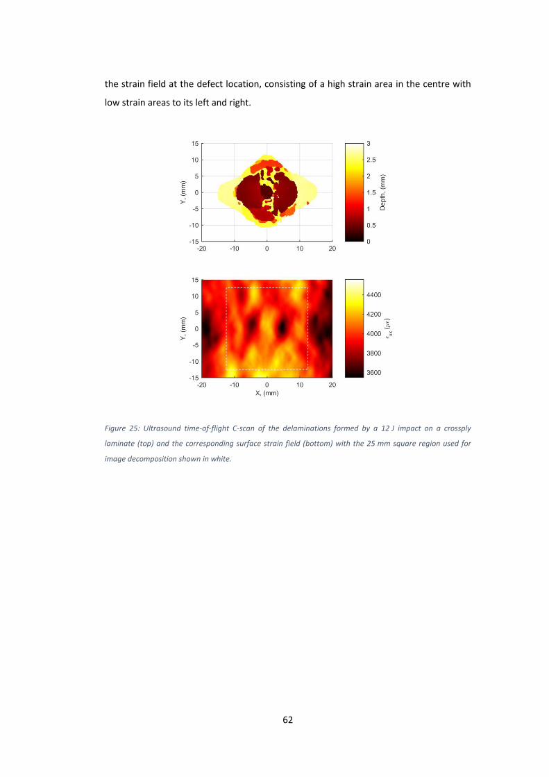
62

the strain field at the defect location, consisting of a high strain area in the centre with

low strain areas to its left and right.

Figure 25: Ultrasound time-of-flight C-scan of the delaminations formed by a 12 J impact on a crossply

laminate (top) and the corresponding surface strain field (bottom) with the 25 mm square region used for

image decomposition shown in white.

63

Figure 26: Ultrasound time-of-flight C-scan of the delaminations formed by a 12 J impact on a quasi-isotropic

laminate (top) and the corresponding surface strain field (bottom) with the 25 mm square region used for

image decomposition shown in white.

The magnitude of the strain pattern caused by the impact damage can be seen to

vary with impact energy. As the impact energy was increased, the pattern become clearer.

This can be seen for crossply and quasi-isotropic coupons in Figure 27 and Figure 28

respectively.

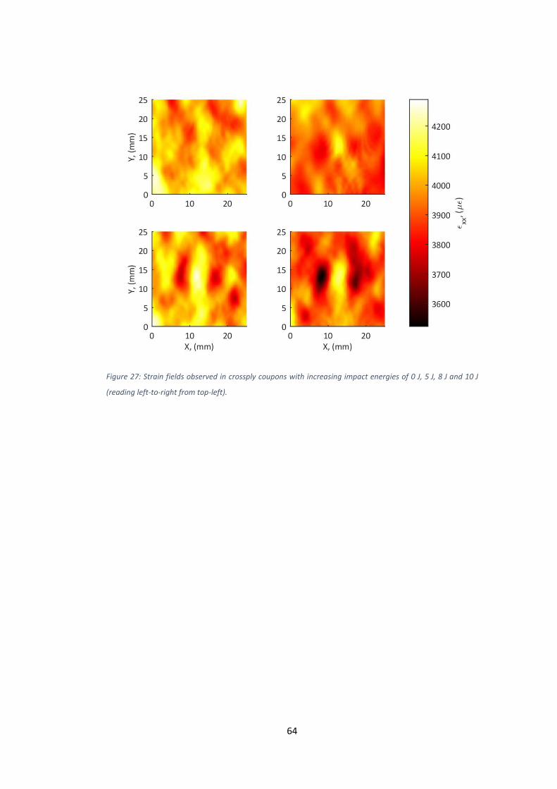
64

Figure 27: Strain fields observed in crossply coupons with increasing impact energies of 0 J, 5 J, 8 J and 10 J

(reading left-to-right from top-left).

65

Figure 28: Strain fields observed in quasi-isotropic coupons with increasing impact energies of 0 J, 5 J, 10 J and

15 J (reading left-to-right from top-left).

For the strain-based defect assessment to be performed, data from a virgin

coupon was required as a reference. For the crossply coupons, only one virgin coupon was

available and this was used for comparison with the defective crossply coupons. For the

quasi-isotropic coupons, there was data from six virgin coupons and thus, the most

suitable had to be selected as the reference strain field against which to compare the

defective coupons. Some variability was observed in the failure load for the six virgin

quasi-isotropic coupons, as shown in Table 4. The ultimate bending moments for the six

coupons had a mean of 52.95 Nm and standard deviation of 4.96 Nm; however, it was

clear that the failure load for coupon RC4 was substantially lower than for the other five

coupons. The maximum normed residual technique, a method of identifying outliers

described in [14], was used and confirmed that RC4 was an outlier. This indicated that RC4

was unsuitable for use as the reference coupon. The mean and standard deviation of the

five virgin quasi-isotropic coupons, excluding RC4, were found to be 54.95 Nm and

1.01 Nm respectively and no further outliers were identified. Coupon RC1 had a failure

load closest to the mean and, hence, it was chosen as the reference coupon for the quasi-

isotropic coupons.

66

Table 4: Ultimate bending moments for the six virgin quasi-isotropic coupons.

Coupon

Identifier

Ultimate Bending

Moment (Nm)

RC1 55.08

RC2 53.89

RC3 55.23

RC4 42.99

RC5 56.42

RC6 54.11

Robust Bayesian linear regression, described in Chapter 4, was used to fit a

predictive function for the residual strength to the measured defect severities. Four

regression models were constructed for each batch of coupons making predictions based

on: the defect area measured using ultrasound, the Manhattan distance between feature

vectors, Pearson dissimilarity between feature vectors and Euclidean distance between

feature vectors. The defect area measured using ultrasound was shown to be the most

effective ultrasound metric for use in residual strength predictions in Chapter 4 and

therefore is the only ultrasound defect measurement used in this chapter. The

construction of the four regression models per batch of coupons allowed a direct

comparison of the predictions generated using each of the measurements. The

measurements and the fitted regression models for the defect assessments using defect

area and Manhattan distance are shown in Figure 29 and Figure 30. These regression

models could be used to generate predictions of the residual strength of defective

components made from an identical laminate found to contain impact damage. The

credible interval around the line-of-best-fit, shown as the grey region on the graphs in the

two figures, indicates the range of most probable residual strength values that could be

exhibited by a laminate with a measured defect severity. The probability that the true

residual strength would be contained in the credible interval is 95% and thus the lower

bound of the interval could be used as a conservative estimate of residual strength with

only a 2.5% chance that the residual strength would be lower.

67

Figure 29: Regression models relating defect severity measurements to the residual strength of defective

crossply composites using the ultrasound-based defect severity (top) and the Manhattan distance for strain-

based assessments (bottom).

68

Figure 30: Regression models relating defect severity measurements to the residual strength of defective

quasi-isotropic composites using the ultrasound-based defect severity (top) and the Manhattan distance for

strain-based assessments (bottom).

Patki and Patterson used three defect severity metrics when performing strain-

based assessments [5]. These were the Euclidean distance, Pearson dissimilarity, and

cosine dissimilarity. For continuity, these defect metrics were also explored in this study.

As previously discussed, when comparing two feature vectors of Tchebichef shape

descriptors, the cosine similarity and Pearson correlation are close to identical. When

plotting the results there was no discernible difference between the values obtained with

either metric and no difference in prediction accuracy. Therefore, only the Euclidean

distance and Pearson dissimilarity are plotted in Figure 31 and Figure 32.

69

Figure 31: Strain-based defect assessments of crossply coupons using Pearson dissimilarity (top) and Euclidean

distance (bottom).

70

Figure 32: Strain-based defect assessments of quasi-isotropic coupons using Pearson dissimilarity (top) and

Euclidean distance (bottom).

To make quantitative comparisons between the predictive capabilities of the

models based on ultrasonic and strain-based defect assessments, it was necessary to

calculate their average prediction uncertainty. This was achieved by calculating the

LOOCV performance metric introduced in Chapter 4. The best performing defect

assessment technique would have the lowest value of the LOOCV performance metric,

because it is a measure of the average prediction uncertainty. The performance metrics

for the ultrasound and strain-based defect predictions are shown in Table 5.

71

Table 5: The LOOCV performance metrics for the ultrasound-based predictions and the strain-based

predictions of residual strength for crossply and quasi-isotropic laminates.

Coupon Layup LOOCV of

Ultrasound-based

Predictions (Nm)

LOOCV of Strain-based Predictions (Nm)

Manhattan

Distance

Euclidean

Distance

Pearson

Dissimilarity

Crossply 2.96 0.97 2.79 1.85

Quasi-isotropic 5.84 4.43 7.19 5.33

5.5. Discussion

The ultrasound time-of-flight C-scans of the defects in both the crossply and

quasi-isotropic coupons have been used to measure the projected defect area caused by

the drop-weight impactor. There is more noise evident in the C-scans of the defects in the

crossply than the quasi-isotropic laminates. This noise is likely caused by areas of fibre-

breakage that are more likely in the crossply material and which, unlike delaminations,

cause the ultrasound energy to scatter rather than be reflected back to the probe. The

strain-field is not adversely affected by different failure modes and thus the noise in the

data is uniform regardless of the modes present. A characteristic pattern can be observed

in the strain data for impacted laminates, shown in Figure 25 and Figure 26. This

characteristic pattern becomes more visible as the energy of impact increases, this can be

seen in Figure 27. The Manhattan distances between feature vectors representing the

strain fields in the defective coupons and the reference virgin coupon were then

calculated and used as the strain-based measure of defect severity. When the Manhattan

distance was plotted against the residual strength of the defective coupons, as show in

the bottom of Figure 29 and Figure 30, a strong linear correlation was observed. A linear

correlation was also observed for the ultrasound-based defect severity measurements;

but, the spread of data points around the line-of-best-fit was much wider, and thus,

predictions based on this ultrasound data would be less accurate. As Patki and Patterson

used the Euclidean distance and Pearson dissimilarity metrics for strain-based defect

assessments, these metrics have also been used in this study. A linear correlation can be

observed between the two defect metrics and the residual strength in Figure 31 and

Figure 32.

72

The predictive power of the three strain based defect metrics and the single

ultrasound-based regression models were assessed using the LOOCV performance metric,

which estimates the average prediction uncertainty of each of the regression models. Of

the three strain-based defect metrics, the Manhattan distance was, as expected, the most

effective for predicting the residual strength of the defective coupons. As the predictions

of residual strength were the most accurate when using the Manhattan distance, this is

the dissimilarity metric recommended to compare feature vectors of shape descriptors

for a strain-based defect assessment. When the LOOCV performance metrics were

compared for the crossply coupons, the average prediction uncertainty was found to be

approximately three times larger for ultrasound-based predictions than the

corresponding uncertainty for strain-based predictions using the Manhattan distance.

This indicates that the strain-based methodology represents a substantial improvement

in ability to assess the severity of a defect compared to ultrasonic measurements. Thus, if

the strain-based defect assessment was used in place of an ultrasound-based method

then a reduction in the number of components being unnecessarily repaired or replaced

could be expected. Although, for other defect types ultrasound or thermography may still

be the most appropriate inspection technique. When comparisons are made between the

ultrasound and strain-based LOOCV metrics for the quasi-isotropic coupons, a similar

decrease in uncertainty is evident; however, the LOOCV metric for ultrasound-based

predictions is 1.32 times more than for the strain-based predictions using the Manhattan

distance. This difference in performance may be due to the distribution of delaminations

in the two different laminates, but still represents a significant increase in the accuracy of

predictions.

For strain-based defect assessments to be applied to aerospace structures, strain

must be induced within the inspected components. This is likely to be the most significant

hurdle for the application of this technique, as the induced strain must exceed the

minimum resolution of the measurement system. For an elastic material, the magnitude

of the strain-field varies linearly with the applied load, thus the value of the shape

descriptors representing that strain field also have a linear relationship with load [48]. The

Manhattan distance between two feature vectors therefore scales with the load used to

induce the strain fields that the feature vectors represent. And, the ability for the strain-

based defect assessment to measure small values of Manhattan distance is related to the

measurement uncertainty of the DIC system. The DIC system used in this thesis was found

73

to have a measurement uncertainty of 44 μϵ. A lower strain measurement uncertainty of

29 μϵ has been achieved using a similar measurement system [79] and a DIC system from

a different manufacturer was found to have a measurement uncertainty of 30 μϵ [53]. The

higher uncertainty of the DIC system used in this thesis is likely due to the high stereo

angle of the cameras, resulting in a reduction in the accuracy of in-plane measurements

[77]. Defects that cause the strain field to vary with a Manhattan distance close to the

measurement uncertainty would be indistinguishable from a virgin coupon. This is not

necessarily a significant problem for structural assessments, as such a defect would not

be expected to reduce the residual strength of the composite. For instance, if one of the

crossply coupons contained a through-width delamination, then the bending moment at

which the delamination propagates, 𝑀𝑝, and the amount the strain field is affected by the

delamination, ∆𝜖, can be estimated using a simple one-dimensional model based on

buckling [90, 91].

When using the model, the bending moment at which the delamination would

propagate, 𝑀𝑝, can be estimated in terms of the delamination length, 𝐿𝑑. In the model,

the strain energy release rate, 𝐺𝐼, is related to the axial strains in the material at the

delamination when buckling occurs, 𝜖𝑏, and when propagation occurs, 𝜖𝑑, by:

22

𝐺𝐼 =𝐸𝑎𝑡

2(𝜖𝑑 − 𝜖𝑏)(𝜖𝑑 + 3𝜖𝑏) (22)

where 𝐸 is the elastic modulus of the laminate calculated from data in [54], 𝑎 is the ratio

of ply thickness to laminate thickness and 𝑡 is the laminate thickness. 𝜖𝑏, the axial strain

at which the material below the delamination would buckle, is given by [91]:

23

𝜖𝑏 =𝜋2𝑎2𝑡2

3𝐿𝑑2 (23)

and, 𝜖𝑑, the axial strain at the delamination when propagation occurs, can be calculated

by assuming simple bending and based on [91]:

24

𝜖𝑑 =6𝑀𝑝

𝐸𝑤𝑡2(1−𝑎)2 (24)

where 𝑤 is the coupon width and 𝑀𝑝 is the bending moment at which propagation occurs.

The parameters for Equations (22), (23) and (24) are defined in Table 6, with the material

properties taken from [54] and dimensions based on the crossply coupons tested in this

74

chapter. The bending moment at which the delamination starts to propagate can then be

calculated by finding the roots to the quadratic in Equation (22).

Table 6: Parameters used for predicting the propagation loads for a through thickness laminate.

Parameter Value

𝐺𝐼 550 N/m [54]

𝐸 76.7 GPa

𝐸𝑑𝑎𝑚 71.2 GPa

𝑎 111⁄

𝑡 3 mm

𝑤 40 mm

𝐿𝑖 25 mm

By using Equations (22), (23) and (24), the bending moment at which propagation

occurs can be obtained for any length of delamination. However, to demonstrate that

insignificant defects have only a minimal effect on the strain field, the propagation

bending moment needs to be related to how much the strain field is affected by the

delamination. Thus, the amount of change to the strain-field in the inspected square area,

at an applied inspection bending moment, 𝑀𝑖 = 20 Nm, was estimated. To achieve this, it

was assumed that the delaminated 0⁰ ply does not contribute to the stiffness of the

coupon, resulting in a reduced modulus of elasticity, 𝐸𝑑𝑎𝑚, due to the missing ply, and a

reduction in the coupon thickness. The strain on the coupon surface at a delaminated

location can then be calculated using simple bending as:

25

𝜖𝑖,𝑑 =6𝑀𝑖

𝐸𝑑𝑎𝑚𝑤𝑡2(1−𝑎)2 (25)

which would be higher than the surface strain at a virgin location, given by:

26

𝜖𝑖,𝑣 =6𝑀𝑖

𝐸𝑤𝑡2 (26)

75

The amount the mean surface strain has changed from a virgin coupon can then be

calculated using the strains given by Equations (25) and (26) and the size of the

delamination relative to the size of the inspected area, 𝐿𝑖. The strain difference, ∆𝜖,

between a virgin and a defective coupon can therefore be calculated as:

27

∆𝜖 =𝐿𝑑

𝐿𝑖(𝜖𝑖,𝑑 − 𝜖𝑖,𝑣) (27)

Hence, the bending moment required to cause propagation can be calculated for a range

of different sized delaminations and plotted against the change in the strain field, as

shown in Figure 33. The vertical line in Figure 33 indicates the smallest measurable strain

difference between a virgin and defective coupon, which was set to the 95% confidence

interval for strain measurement using the DIC system, which is equal to four times the

system measurement uncertainty. Therefore, Figure 33 shows that a delamination that

does not result in a measurable change to the strain-field, i.e. to the left of the dashed

line, would not be expected to propagate and does not reduce the residual strength of

the coupon. Consequently, if the difference in the strain-field between the virgin and

defective states is less than the measurement resolution of the DIC system, the defect can

be ignored.

Figure 33: The moment, 𝑀𝑝, to cause propagation of a delamination (solid line) as a function of the strain

difference, ∆𝜖, relative to a virgin coupon, developed around the delamination when an inspection moment of

20 Nm is applied (dotted line). The graph indicates the inspection moment will not induce propagation and

the minimum measurable strain difference (dashed line) corresponds to a delamination that will only

propagate due to a moment larger than the ultimate moment of the virgin coupon (chain line).

76

For ultrasonic assessments, the size of a detectable defect is closely linked with the

resolution of the assessment technique, but the size of defect does not indicate the risk

associated with the presence of that defect. For instance, a small delamination in a highly-

stressed area of a structure would likely cause a greater reduction in residual strength

than a large delamination in a low-stressed area, but the ultrasound inspection is more

likely to detect the large delamination. This could lead to defects being missed that could

significantly reduce the strength of a structure whilst large defects, that may be

insignificant, are detected. With a strain-based inspection, there is a correlation between

how the defect affects the residual strength and how much it changes the strain-field.

Therefore, undetectable defects would not be expected to affect the residual strength

and can be safely ignored. The required measurement uncertainty for a strain-based

assessment can be defined by considering the minimum residual strength of the defective

structure. This means that for a strain-based inspection the required measurement

resolution is simple to define, and may lead to fewer situations where critical defects are

missed.

5.6. Conclusions

A novel method of assessing defective composites with measurements of the

resulting strain field has been used to make predictions of the residual strength of crossply

and quasi-isotropic carbon fibre composite coupons with barely visible impact damage

(BVID). A large number of coupons were manufactured and impact, with a known level of

impact energy, applied using a drop-weight impact tower. The coupons were then loaded

in bending to induce strain and full-field strain data captured using digital image

correlation. The dimensionality of the strain fields was reduced using image

decomposition resulting in feature vectors that represent the strain on the surface of each

coupon. The defects were quantified by numerically comparing the feature vector for

each defective coupon with the feature vector for a virgin coupon using three different

dissimilarity metrics: Euclidean distance, Pearson dissimilarity and Manhattan distance.

Each of these dissimilarity metrics resulted in a strain-based measure of defect severity

that was found to linearly correlate with the residual strength of the defective coupons.

An ultrasound-based defect assessment was also performed on the coupons allowing for

a direct comparison between the new methodology and an established inspection

technique.

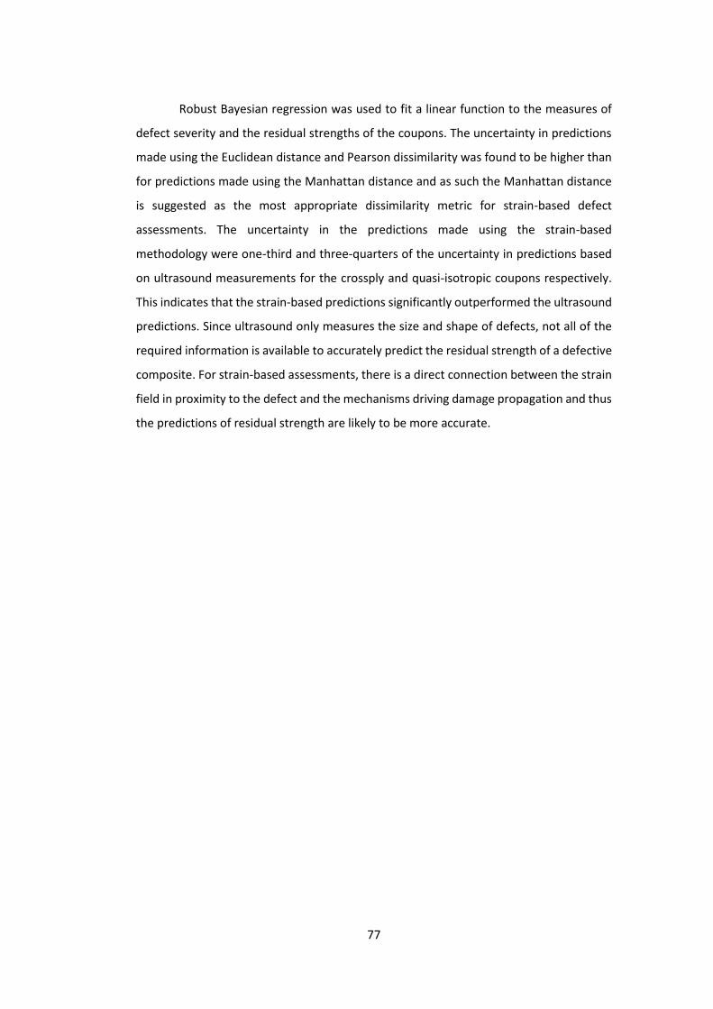
77

Robust Bayesian regression was used to fit a linear function to the measures of

defect severity and the residual strengths of the coupons. The uncertainty in predictions

made using the Euclidean distance and Pearson dissimilarity was found to be higher than

for predictions made using the Manhattan distance and as such the Manhattan distance

is suggested as the most appropriate dissimilarity metric for strain-based defect

assessments. The uncertainty in the predictions made using the strain-based

methodology were one-third and three-quarters of the uncertainty in predictions based

on ultrasound measurements for the crossply and quasi-isotropic coupons respectively.

This indicates that the strain-based predictions significantly outperformed the ultrasound

predictions. Since ultrasound only measures the size and shape of defects, not all of the

required information is available to accurately predict the residual strength of a defective

composite. For strain-based assessments, there is a direct connection between the strain

field in proximity to the defect and the mechanisms driving damage propagation and thus

the predictions of residual strength are likely to be more accurate.

78

6. Manufacture and Characterisation of In-plane Fibre-

waviness Defects

6.1. Introduction

Carbon-fibre composite materials exhibit high levels of specific strength along the

fibre direction. However, if instead of having the desired orientation, there are

unintended local variations in orientation, the material can be substantially weaker than

the design strength. This variation in alignment is termed fibre-waviness, as the shape of

the misaligned fibres are often approximately sinusoidal. Fibre-waviness can be split into

two forms: out-of-plane, where the plies in the laminate are misaligned in the thickness

direction; and in-plane, where the fibres within a ply are misaligned [64]. Waviness has

the effect of locally reducing both the stiffness and the strength of the plies and

consequently the limit load for the component. Since fibre-waviness could threaten the

safety of a structure, it is important to explore how such a defect affects the load-bearing

characteristics of a structure.

During the literature review, methods of producing in-plane fibre-waviness were

identified. One promising technique [64] was to lay prepreg plies over a flexible curved

surface. Once the laminate was laid-up, the curved surface was then flattened. This

caused the fibres on the upper surface of the laminate to buckle, resulting in coupons with

high levels of in-plane fibre-waviness uniformly distributed throughout the laminate.

However, to develop an inspection technique, it is necessary to have a localised defect.

This is to demonstrate that the assessment can locate defects and thus be classified as at

least a Level 2 technique when using Rytter’s classifications [1]. Localised defects also

ensure that the defect is far away from load application points. This prevents interactions

between the contact forces and the defect leading to premature failure. For this study, a

new technique was developed for creating localised waviness defects based on [64]. The

defects produced by the new manufacturing technique were then characterised using: an

established ultrasonic technique to measure the orientation of fibres, a novel technique

involving residual strain measurements, and the strain-based defect assessment applied

in Chapter 5. Whilst a technique for measuring the fibre-orientation using ultrasound has

previously been developed [65], a method of linking such measurements to residual

strength is still required. Therefore, a simple ultrasound-based defect severity metric for

79

fibre-waviness is introduced. This metric allows for the severity of waviness in an area to

be quantified with a single value. Predictions of residual strength were then made using

the statistical framework in Chapter 4 and comparisons made between the strain-based

predictions and ultrasound-based predictions.

This chapter is based on a paper entitled, “Experimental Methods for the

Manufacture and Characterisation of In-plane Fibre-waviness Defects” intended for

submission to Composites Part A: Applied Science and Manufacturing.


6.2.1. Fabrication of Coupons Containing Waviness Defects

Quasi-isotropic laminates were produced with six levels of waviness severity. Six

coupons were produced at each level to explore the variability of the defect generation

technique. This resulted in a large set of 36 coupons. The laminates were manufactured

using RP507UT210 (PRF, UK) unidirectional prepreg with a [02/902/452/-452]S layup. This

is the same layup that was used for the impacted quasi-isotropic coupons in Chapter 5.

Each level of waviness was produced using a milled aluminium former. The profile of each

former had an arc at its centre from which flat surfaces extended on either side, a

photograph of one former is shown in Figure 34. Prepreg plies were laid up over each

former so that the plies closest to the arc surface of the former have a shorter path than

the plies further from the arc surface. Once the prepreg laminate was laid up it was

removed from the former and flattened between two plates using only minimal force

provided by hand. In this uncured state, the laminates had a nominal thickness, 𝑡𝑢, of

3.65 mm. When the prepreg laminates were flattened, the fibres in the plies on the top

surface buckled to accommodate the constraint within the flattened laminate. These

buckled fibres are the cause of the in-plane fibre-waviness. The severity of the waviness

in the uncured laminates produced by each former was quantified by the percentage

reduction in length when curved, 𝑙𝑐𝑢𝑟𝑣𝑒𝑑 , to their length when flattened, 𝑙𝑓𝑙𝑎𝑡, of the

fibres on the top of the laminate at the arc section. This can also be expressed in terms of

the arc radius, 𝑟, and uncured laminate thickness, 𝑡𝑢, as:

28

𝑁𝑜𝑚𝑖𝑛𝑎𝑙 𝑊𝑎𝑣𝑖𝑛𝑒𝑠𝑠 = 𝑙𝑐𝑢𝑟𝑣𝑒𝑑−𝑙𝑓𝑙𝑎𝑡

𝑙𝑐𝑢𝑟𝑣𝑒𝑑=

𝑡𝑢

𝑟+𝑡𝑢 (28)

80

By varying the angle between the flat surfaces extending from either side of the arc in the

former, the arc length and thus the length of the waviness defect can be controlled. The

arc length for all coupons was kept constant at 20 mm. The six levels of nominal waviness

chosen were: 0%, 10%, 15%, 17.5%, 20% and 25%. The arc radii and angle between the

two flat surfaces for the five formers are listed in Table 7.

Figure 34: Photograph of a former for creating coupons with a nominal waviness of 15%.

Table 7: Key dimensions of the formers to obtain various levels of nominal waviness over a 20 mm length of

coupon.

Nominal Waviness, (%) Arc radius, 𝒓, (mm) Corner angle, (⁰)

10.0 32.9 145.1

15.0 20.7 124.6

17.5 17.2 113.4

20.0 14.6 101.5

25.0 11.0 75.4

Then, the laminates were cured between flat plates in a hot press (APV-3530,

Meyer, Germany) according to the manufacturer’s instructions. The cure was conducted

over 45 minutes at a temperature of 130 °C. The press applied a constant pressure of

2.5 bar to the laminates whilst heating, curing and cooling. Once the laminate was cured,

the hot press was left to cool to room temperature at a natural rate. The laminates were

then cut into 40 by 220 mm coupons using a wet diamond saw (Versatile 103450, Vitrex,

81

USA). Care was taken to ensure the long edge of the coupons was parallel to the 0°

direction of the fibres and that the wavy area was close to the coupon centre. This

resulted in the 0⁰ fibres in the top and bottom plies running parallel to the X-direction for

measurements, indicated on Figure 35.

Figure 35: Photograph of a coupon with a nominal waviness of 25%, showing the speckle pattern and

measurement coordinate system.

To examine the effect of high levels of waviness, two coupons were produced

with the top 0⁰ plies replaced with 90⁰ plies. This corresponds to the worst possible case

of fibre-waviness as it is the complete misalignment of fibres and thus was used to

determine how much the ultimate bending moment can be reduced due to fibre-

waviness. These coupons were cured using the same process described previously and cut

to the same size as the other coupons.

6.2.2. Ultrasonic Characterisation

Each coupon was inspected using the pulse-echo ultrasound technique described

in Chapter 3. For the inspection, the gate on the ultrasonic flaw detector was positioned

to detect only the echoes that came from the first ply interface, which is immediately

below the ply containing the waviness defect. The amplitude of the peaks passing through

the gate were recorded resulting in amplitude C-scans of the defect. The fibre bundles in

the 0° ply were visible in the texture within the C-scans and thus, the local orientation of

the fibres could be measured. This was achieved by performing the 2D discrete Fourier

transform on square subsets of the C-scan. The subset size used was 75 pixels (7.5 mm)

and the subsets had a spacing of 10 pixels (1 mm). Prior to calculating the Fourier

transform of the subset, a radial Hann window was applied, this limits spectral leakage

which would cause the peak at the centre of the spectral image to broaden [65]. A

windowed subset is shown at the top of Figure 36. The power spectrum image obtained

had a roughly elliptical shape at its centre which was at right angles to the orientation of

82

the texture in the spatial image, as shown at the bottom of Figure 36. Thus, by measuring

the orientation of the power spectrum ellipse, the local fibre-orientation was obtained.

This technique, of using ultrasound to measure fibre-orientation, is described in detail in

[65].

Figure 36: A subset with applied Hann window (top) and its spectral image (bottom) taken from an amplitude

C-scan of a waviness defect in a 17.5% nominal waviness coupon.

6.2.3. Digital Image Correlation and Thermoelastic Stress Analysis of Waviness

Coupons

TSA was performed on one coupon at each level of nominal waviness, six in total.

The opposite surface of the coupon to the waviness defect was inspected, with the

inspected surface constantly in tension and the defective surface in compression. A

60 mm by 40 mm section of each coupon was sprayed matte black in order to perform

83

the TSA analysis described in Chapter 3. The coupons were loaded under displacement

control as the force applied by the load machine was intended to be low relative to the

range of its load cell. A cyclic displacement of ±0.3 mm with a mean displacement of

0.5 mm was applied at 20 Hz. This is equivalent to a cyclic load of ±1 Nm, with a peak load

of 2.67 Nm. An integration time of 10 minutes was used to increase the signal-to-noise

ratio of the thermoelastic signal. Once TSA inspections had been performed, these

coupons were resprayed with a speckle pattern to enable a direct comparison between

the two measurement techniques.

DIC was used to measure strain on the surface of all the waviness coupons. A

speckle pattern was applied to a 60 by 40 mm section of each coupon at the location of

the fibre-waviness defect on the opposite surface to the defect, a sprayed coupon is

shown in Figure 35. The coupons were then loaded in the four-point bending rig, so that

the defective ply was placed into compression when loaded. The coupons were first

inspected using the strain-based defect assessment described in Chapter 5. Subsequently,

the coupons were loaded to failure whilst DIC was used to observe the progression to

failure. For the tests to failure, the lower half of the bending rig was moved towards the

upper load noses at a constant displacement rate of 0.8 mm/min. The DIC system was set

to capture images every 15 s, this resulted in a bending-rig displacement of 0.2 mm

between each image. The test was stopped when the stiffness of the coupon was reduced

to approximately half its initial value.

6.3. Results

After the laminates were cured and cut into coupons it was observed that despite

being cured between flat plates, the coupons were slightly curved along their length in

the X-direction. This curvature was caused by residual strains in the laminate. As the

curvature of the coupons was small, the residual strains in the coupons that caused the

curvature were determined from the out-of-plane displacements [92]. The residual strains

in the direction along the length of the coupon were calculated as:

29

𝜖𝑥,𝑟𝑒𝑠 = −𝑡𝑐

2

𝜕2𝑤

𝜕𝑥2 (29)

where 𝑡𝑐 is the cured thickness of the laminate and 𝑤 is the displacement of the defect-

free surface from a flat plane. For each coupon, the DIC reference image was processed

84

to measure the shape before any loads were applied, resulting in the data as shown at

the top of Figure 37. The second partial derivative of this shape data was then calculated

using the central difference method [92] with a step size of 8 mm, resulting in the residual

strain field shown at the bottom of Figure 37.

Figure 37: DIC measurements of the surface deviation from a flat plane for an unloaded coupon with a nominal

waviness of 17.5% (top) and the associated residual strain field (bottom).

The fibre-waviness was apparent; in the ultrasound data, in the DIC strain when

the coupons were loaded, and also, in the residual strain maps when no load was present.

It was also possible to identify the same spatial distribution of the waviness defect in each

coupon using the three distinct inspection techniques. Data from a coupon that had a

nominal waviness of 25% is shown in Figure 38. A strip of highly wavy fibres is visible

across the width of the coupon, at x = -2 mm in the ultrasound data, and a corresponding

area of high strain is visible in the strain field and the residual strain field. A less severe

strip of waviness is also visible in all three data sets, at x = 17 mm.

85

Figure 38: A coupon that had a nominal waviness of 25%, inspected with: ultrasound (top), surface strain at a

load of 22 Nm (middle) and residual strain measurements (bottom).

The overall waviness measured using ultrasound was quantified by calculating the

root mean square (RMS) of the fibre orientation fields. By calculating the RMS of the

ultrasound data, both local misalignment due to the waviness defect and any gross

misalignment of the plies was quantified. When waviness was present, a correlation

between the nominal waviness and the RMS of the measured waviness was observed and

is shown in Figure 39. Piecewise robust Bayesian regression, described in Chapter 3, was

used to determine a function linking the nominal waviness to the measured waviness

86

severity after curing. The grey region shown in Figure 39 is the 95% credible interval and

indicates the most probable range of the measured waviness after curing for a given

nominal waviness.

Figure 39: The ultrasound measured waviness for coupons after curing for six different levels of nominal

waviness.

The ultimate bending moment of the coupons containing fibre-waviness was also

found to correlate with the RMS of the measured waviness, as shown in Figure 40. A linear

correlation between the measured waviness and ultimate bending moment was observed

when the measured waviness was less than 10⁰. When the measured waviness was above

10⁰, the coupons failed with an average ultimate bending moment of 27.7 Nm, regardless

of the measured value of waviness. The two coupons with the top 0⁰ plies replaced by 90⁰

plies were loaded to failure and found to fail at 30.3 and 29.4 Nm. These coupons had an

RMS of measured waviness of 90⁰. The effectiveness of using ultrasound measurements

of waviness to predict the strength of laminates was then explored. Coupons with an RMS

of waviness below 10⁰ were used to fit two robust Bayesian linear regression models, as

described in Chapter 4. The input for the regression models were: the RMS of ultrasound

measured waviness, and the mean of the residual strain field. It was clear from the graphs

87

of the two fitted regression models, in Figure 41, that both measurements have a strong

linear correlation with the ultimate bending moment. The average prediction uncertainty

of the two regression models was estimated using the LOOCV performance metric. The

average prediction uncertainty was 3.94 Nm for ultrasound-based predictions and

2.24 Nm for predictions based on residual strain measurements.

Figure 40: The effect of waviness after curing on the ultimate bending moment for all coupons.

Figure 41: Graphs for predicting the ultimate bending moment of coupons using RMS of waviness measured

with ultrasound (left) and the mean of the residual strain field (right).

88

The strain-based defect assessment conducted in Chapter 5 was also conducted

on the same reduced set of waviness specimens. A correlation was observed between the

Manhattan distance and the residual strength, shown Figure 42. The average prediction

uncertainty for the strain-based defect assessment of fibre-waviness specimens was

5.32 Nm.

Figure 42: Predictions of residual strength made using the strain-based defect assessment technique for fibre-

waviness coupons.

TSA was also performed on six of the waviness coupons, with one coupon at each

level of nominal waviness inspected. The thermoelastic signal fields for the six waviness

coupons are shown in Figure 43. The DIC strain-fields for the same coupons are shown in

Figure 44. These strain-fields are of the first strain invariant, which would be directly

proportional to the thermoelastic fields if the material was isotropic. Similarities can be

observed between the patterns visible in the TSA data, shown in Figure 43, and those

measured using DIC, in Figure 44. The same pattern can be observed in the two images

for the 25% nominal waviness coupon and hotspots at the same locations in both figures

can be identified for the 17.5% and 20% nominal waviness coupons.

89

Figure 43: Full field maps of the thermoelastic signal for six waviness coupons. Colour is used to show the

magnitude of the thermoelastic signal in raw camera units.

90

Figure 44: DIC strain fields of fibre-waviness defects. Colour indicates the magnitude of surface first strain

invariant.

Image decomposition was used to quantify the similarities in shape between the

two data sources. First, a 35 mm wide square section of each of the TSA and DIC images

was selected. Image decomposition was conducted on each of these square images. For

the decomposition process, shape descriptors corresponding to the Tchebichef image

moments up to an order of ten were computed. The first shape descriptor for each feature

vector was discarded as it is always equal to the mean of the image it represents and thus,

does not contain useful information for shape analysis. The DIC and TSA shape descriptors

were then plotted against each other as a scatter diagram, as shown by crosses at the

bottom of Figure 45. The line-of-best-fit for the shape descriptors, calculated using least-

squares regression, is also shown. The Pearson correlation was calculated for each pair of

feature vectors representing the TSA and DIC data for a single coupon. If the shapes in the

TSA and DIC data were identical, then the Pearson correlation would be equal to 1. If there

was no correlation between the data then the value would be approximately 0. The

Pearson correlations for the six coupons are shown in Table 8.

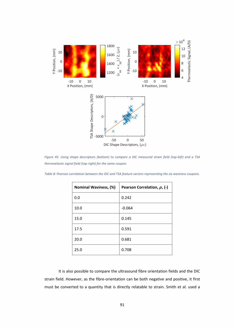
91

Figure 45: Using shape descriptors (bottom) to compare a DIC measured strain field (top-left) and a TSA

thermoelastic signal field (top-right) for the same coupon.

Table 8: Pearson correlation between the DIC and TSA feature vectors representing the six waviness coupons.

Nominal Waviness, (%) Pearson Correlation, 𝝆, (-)

0.0 0.242

10.0 -0.064

15.0 0.145

17.5 0.591

20.0 0.681

25.0 0.708

It is also possible to compare the ultrasound fibre orientation fields and the DIC

strain field. However, as the fibre-orientation can be both negative and positive, it first

must be converted to a quantity that is directly relatable to strain. Smith et al. used a

92

fibre-orientation field to modify an FE model of a component [71]. The same methodology

can be used with the data collected in this study to convert ultrasound measurements of

waviness into predictions of strain on the tensile surface of the coupons. A generic model

of the coupons used in this study was created in Abaqus 6.14 (Dassault Systems, France)

using 136,960 brick elements (type C3D8R) of which 76,800 elements formed a dense

mesh at middle of the simulated coupon, the mesh is shown in Figure 46. This model used

the material properties given by Gong et al. [54] for a similar composite. The fibre-

orientation field measured using ultrasound was then used to define the material

orientation for the individual elements of the model corresponding to the same location

as in the physical coupon. The strain field on the surface of the simulated coupon was

then predicted for a bending-rig displacement of 5 mm.

Figure 46: Abaqus FE mesh of a fibre-waviness coupon during a four-point bend.

Comparisons of the simulated and measured strain fields for each waviness

coupon were then made using the validation technique outlined in CEN Workshop

Agreement 16799:2014 [52]. Shape descriptors up to an order of ten were used to

describe the simulated and measured strain-fields for each coupon which were then

compared, the validation diagram for one coupon is shown in Figure 47. The model was

validated for 34 out of 36 coupons. The two coupons that were not validated were a 20%

and a 25% waviness coupon. For these two coupons, the predicted strain at the centre of

the waviness defect was significantly lower than the measured DIC strain.

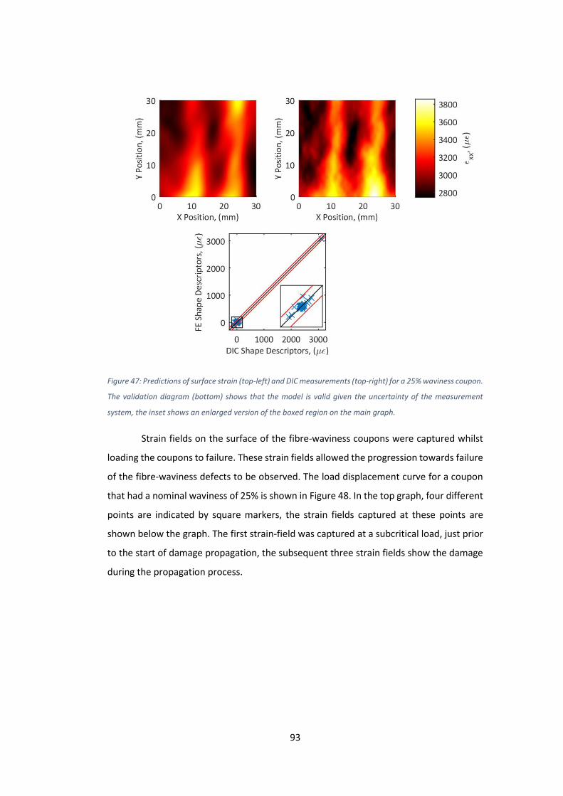
93

Figure 47: Predictions of surface strain (top-left) and DIC measurements (top-right) for a 25% waviness coupon.

The validation diagram (bottom) shows that the model is valid given the uncertainty of the measurement

system, the inset shows an enlarged version of the boxed region on the main graph.

Strain fields on the surface of the fibre-waviness coupons were captured whilst

loading the coupons to failure. These strain fields allowed the progression towards failure

of the fibre-waviness defects to be observed. The load displacement curve for a coupon

that had a nominal waviness of 25% is shown in Figure 48. In the top graph, four different

points are indicated by square markers, the strain fields captured at these points are

shown below the graph. The first strain-field was captured at a subcritical load, just prior

to the start of damage propagation, the subsequent three strain fields show the damage

during the propagation process.

94

Figure 48: Load-displacement graph for a coupon that had a nominal waviness of 25% loaded to failure with

four points on the load curve marked (top) and the strain-fields at these points (bottom).

6.4. Discussion

Waviness defects in composite laminates can be caused by: misalignments in the

unidirectional prepreg tape used to produce the laminate; the geometry of the tooling for

the desired component shape; or the orientation of the reinforcement fibres [93].

Thermal stresses produced during the curing process can also result in waviness defects

[94]. The fibre-waviness defects in this study were produced by inducing axial strain in the

top surface of the uncured laminate causing the fibres to buckle. This is not a typical

process by which fibre-waviness defects occur in industry, but it does result in defects that

95

are reproducible and suitable analogues for the study of both the mechanical behaviour

of the defects and the NDE techniques used to detect them.

Three distinct techniques have been used to inspect all of the coupons. The first

technique was the use of ultrasound to measure the fibre orientation in the top ply of the

coupons, allowing the defects to be located and their severity quantified. The second

technique utilised DIC to measure the strain redistribution due to the waviness defect.

Finally, the curvature of the coupons was used to locate defects. The curvature was

caused by residual stresses in the laminate at the defect location. These residual stresses

are due to the mismatch of thermal expansion coefficients between the laminate layers.

Which, in turn, is due to the orthotropy of the unidirectional plies [95]. If the laminate

layup is symmetric, the stresses produced during cooling are balanced, resulting in a flat

laminate. For this study the laminates had a symmetric quasi-isotropic layup and thus the

residual stresses should be balanced; however, at the waviness defects the fibre

misalignment results in localised areas where the residual stresses are not balanced.

These unbalanced residual stresses and the associated residual strains result in a slight

curvature at the location of the defect. By calculating the second partial derivative of the

out-of-plane displacement these unbalanced residual strains can be evaluated and the

residual strain-fields obtained, as shown at the bottom of Figure 37 and Figure 38. The

shape data used for calculating the residual strain-fields was measured by the same DIC

system used to calculate surface strain in the loaded coupons. Whilst the raw data for

these two measurements were obtained from the same source, the processing of the data

is completely different and similar measurements of residual strain would be obtained by

any suitably sensitive shape measurement technique. Similarities in the spatial

distribution of the defects detected by the three inspection techniques were observed for

all coupons with significant fibre-waviness.

A relationship was found between the nominal waviness and the ultrasound

measured waviness after the coupons were cured. When the nominal waviness was over

10%, a linear correlation was observed, with the data points being widely spread above

and below the line-of-best-fit. The spread of data is likely due to the stochastic process by

which the fibres buckle and thus form the defect. When the nominal waviness was low,

no measurable change was observed in the post-cure waviness measurements. By

utilising piecewise-linear robust Bayesian regression the point at which the nominal

96

waviness causes a measurable change in the fibre-orientation can be estimated and

occurs at approximately 7%. This is likely caused by the flexible uncured laminate

expanding during the curing process allowing the fibres to unbuckle and realign with the

ply direction. If the nominal waviness was minor, then the unbuckling could have allowed

the fibres to return to their defect free orientation.

A correlation is evident in Figure 40 between the RMS of the fibre-waviness and

the ultimate bending moment for the coupons. For low levels of measured fibre-waviness,

a linear relation exists between the measured waviness and residual strength. As the

waviness in the coupons increased, this linear correlation ceased and the coupons failed

with a mean value of 27.7 Nm. This is because the stiffness in the gross fibre direction of

the 0⁰ ply containing the defect cannot be reduced to less than the transverse stiffness of

the ply. Two coupons produced with the top 0⁰ ply replaced with a 90⁰ ply demonstrate

the reduction in ultimate bending moment when the stiffness of the defective ply is

decreased to a minimum. The two coupons failed at an average bending moment of

29.9 Nm which is slightly higher than the average failure load for severe fibre-waviness.

This is because the fibre-waviness defect also acts a stress concentrator, causing higher

stresses at the defect than if the stiffness of the ply was uniformly at a minimum.

The correlation between the ultrasound measurements and ultimate bending

moment means that strength predictions can be made using these measurements. The

accuracy of these predictions was quantified only for coupons containing waviness up to

an RMS of 10⁰ as the relation was linear in this range. The mean of the measured residual

strain field was also used as a predictor to examine if the residual strains produced by

waviness are important for predicting ultimate strength. One coupon, with a nominal

waviness of 0%, was observed to have a mean residual strain of -58 μϵ. This coupon had

the highest ultimate bending moment of all the tested coupons. The negative mean

residual strain could have been caused by a thermal gradient through the thickness of the

coupon during curing. As the regression model was robust against outliers, the data from

this coupon was not omitted. When the LOOCV performance metric was calculated for

the two regression models shown in Figure 41, it was found that the predictions obtained

using residual strain measurements had an uncertainty that was only 56% of that for

ultrasound based predictions. This suggests that the residual strains formed at the defect

during curing have a significant effect on the mechanical properties of the laminate, and

97

thus, computational models that attempt to predict the strength of laminates containing

fibre-waviness could be improved by incorporating the residual stresses at the location of

the defect. This also implies that residual strains obtained from optical shape

measurements could be used to locate and quantify the severity of waviness defects, as

long as the laminate has a constant thickness and the defect is not in one of the middle

plies. Although, the equation to calculate residual strain is more complicated when the

specimen is non-flat [92].

The strain-based defect assessment was also conducted on the fibre-waviness

coupons. When observing the graph in Figure 42 it is clear there is more spread in the

values around the line-of-best-fit compared to the graphs in Figure 41. This is confirmed

when considering the LOOCV performance metric which is 5.32 Nm for the strain-based

predictions compared to the 3.94 Nm for the ultrasound based predictions. This indicates

that the strain-based defect assessment conducted in Chapter 5 does not result in a

significant decrease in prediction uncertainty relative to ultrasound-based predictions for

waviness defects. However, it should be noted that the line-of-best-fit is close to those

calculated in Chapter 5. When the fibre-waviness data is plotted on the bottom graph of

Figure 30 the data points corresponding to the waviness coupons are mostly contained

within the credible interval, this is shown in Figure 49. If the regression model that was

fitted to the impact data could perfectly predict the residual strength of the waviness

coupons then 95% of the waviness data points would be expected in the credible interval.

This was not achieved, as only 83% of the waviness data points are contained within the

credible interval calculated using the impact damage data. But, this does indicate that the

parameters for the line-of-best-fit for a composite laminate may be the same regardless

of the type of defect and thus the parameters could be considered as material properties

that could be applied to a wide range of defect types with minimal need for calibration.

Experiments would need to be conducted on a greater number of distinct defect types to

confirm this hypothesis.

98

Figure 49: Strain-based defect assessment graph for impacted quasi-isotropic coupons (crosses) with fibre-

waviness data points (circles) plotted as well.

To explore other potential measurement techniques TSA has been used to

inspect waviness defects in six coupons. To confirm that TSA was able to locate the

defects, comparisons were made between the TSA data and DIC data for the same

coupons. The similarity between the TSA data and the DIC strain-fields were quantified

using image decomposition to obtain feature vectors and then calculating the Pearson

correlation between each pair of vectors. The Pearson correlation was close to zero for

the 0%, 10% and 15% coupons, indicating no discernible similarities between the DIC and

TSA data for those coupons. For the 17.5%, 20% and 25% coupons, the Pearson

correlation was greater than 0.5, suggesting that the data was similar, as shown in Table

8. Although correlations were found, they were not particularly strong. For example, the

correlation was only 0.705 for the 25% waviness coupon. The low values of Pearson

correlation was likely caused by the anisotropy of the composite laminate, and the

measurement noise of the DIC and TSA systems. The captured data, shown in Figure 43,

indicates that the severity of a defect could be measured using TSA, as the magnitude of

the thermoelastic signal increases with nominal waviness. For the TSA inspection, a

maximum load of just 2.67 Nm was sufficient to detect the defect for the 17.5%, 20% and

25% nominal waviness coupons. The defect may be detectable by DIC at lower loads but

it is unlikely to be observable at 2.67 Nm as the DIC measurement noise would be too

high. Therefore, TSA could be used to inspect stiffer structures where high levels of strain

are difficult to apply. As TSA was only conducted on six coupons, it was not possible to

99

determine if the strain-based defect assessment could be performed using TSA data to

make residual strength predictions.

An FE model has been produced for each coupon and strain fields for the tensile

surface of the coupons predicted. This allows for a direct comparison between the DIC

and ultrasound data. The model was validated for all of the coupons except for two. The

two FE models that could not be validated predicted lower levels of strain than was

measured in the DIC strain fields. Despite this, the high number of validated coupons

suggests that the ultrasound technique is capable of almost completely characterising the

waviness defect, which may explain why the ultrasound-based predictions of residual

strength are better than the strain-based predictions. It may be possible to combine the

FE model developed in this study with a fracture mechanics model to predict the failure

of the coupons, this is similar to [54]. However, to create an FE model of an aerospace

component containing waviness and predict its failure load would require excessive

computational resources and probably be unsuitable for industrial applications.

Finally, DIC has been used to observe the progression towards failure of all the

coupons. A typical example of this data for a coupon with a nominal waviness of 25% is

shown in Figure 48. At a subcritical load, strain field ‘a’ showed two strips of approximately

equal levels of strain running parallel to the y-axis at x = -7 mm and x = +7 mm. After strain

field ‘a’ was captured, a crack was observed forming through the 0⁰ ply on the top surface

at x = -7 mm, running parallel to the y-direction. The formation of this crack corresponded

with the end of the linear relation between bending displacement and measured

moment, confirming that damage was being created. This crack caused a substantial

strain concentration that was visible in strain field ‘b’. When the bending moment

reached 12 mm a sudden drop in the stiffness occurred, this corresponded with a

delamination that formed and immediately buckled. The effect of this delamination can

also be observed in strain field ‘c’ with a large area of high strain running between

x = - 18 mm and x = 8 mm. This area of high strain increased in size by growing further in

the negative x-direction as the bending displacement was increased, as can be seen in

strain-field ‘d’. This progression to failure, whereby a crack forms through the 0° ply at the

defect location, from which a delamination grows, was observed in all of the coupons with

a mean residual strain over 40 μϵ.

100

6.5. Conclusions

A method of creating controlled levels of in-plane fibre-waviness in composite

laminates has been developed and used to produce a large number of coupons at six

levels of nominal waviness. This method allows the size, position and severity of the

defect to be controlled and thus is suited for experimental characterisation of waviness

defects that might occur in industry. The manufactured coupons were inspected using

two non-destructive techniques and a novel assessment technique based on residual

strains. By creating a large batch of coupons, the capabilities of the new residual strain-

based inspection technique could be explored and was shown to be capable of both

detecting and characterising waviness defects. Three robust Bayesian regression models,

capable of predicting the ultimate strength of the coupons in bending, were fitted to the

ultrasound, residual strain data and the strain-based defect assessment performed using

DIC. The predictions of ultimate bending moment based on the residual strain

measurements were found to have an uncertainty of just 2.24 Nm, compared to 3.94 Nm

for ultrasound based predictions and 5.32 Nm for the strain-based predictions. This

suggests that residual strains could be used, under certain conditions, to inspect laminates

for waviness defects. It also indicates that residual strains appear to have a significant

effect on the failure of laminates containing waviness defects and thus incorporating

residual strains into computational models of the defect could result in improved

simulations of its behaviour. The use of these new techniques, for creating and

characterising in-plane waviness defects, has the potential to enhance our understanding

of the influence of fibre-waviness defects on the behaviour of composite structures.

101

7. Discussion

The aim of this project was to increase the quality and confidence in residual

strength information gained from the non-destructive evaluation of composite defects

using strain-based inspections, in addition to currently applied ultrasonic practices for

composite structures. The objectives of this project were to:

develop the statistical methods for predicting the remnant properties of defective

structures based on non-destructive measurements.

develop a technique for determining the severity of defects using full-field strain-

data.

demonstrate the effectiveness of strain-based defect assessments relative to

current practices of ultrasonically inspecting aircraft.

This chapter draws together the findings of this research project, relating them to the

objectives of the project and the knowledge gaps identified in Chapter 2. Future work is

suggested at the end of this chapter, which could be conducted to further improve NDE

techniques for the assessment of defects.

7.1. Creating Defects in Composite Coupons

The efforts to complete the second objective of this project could have been

approached theoretically. However, to demonstrate the potential for this technique to be

applied in industry, it was important that substantial experimental work was conducted.

To fully explore the behaviour of a defect assessment technique, specimens that

represent the types of defect encountered by industry were required. These specimens

could then be used to numerically quantify the accuracy of predictions made using the

assessment techniques. Two types of defect in carbon-fibre laminates were explored in

this study. These were impact damage and in-plane fibre-waviness, both of which are

commonly encountered in industry. Well-established techniques of creating impact

damage existed prior to this study [82] and thus this form of defect was created using a

drop-weight tower. This apparatus can be used to produce similar defects in a laboratory,

as those caused by tool drops and hail strikes during the operation of aerospace

structures. In this study, crossply and quasi-isotropic coupons were impacted using a

20 mm diameter tup at a range of energies. In most cases these impact events resulted in

a set of large delaminations, with some of the quasi-isotropic specimens containing

102

40 mm long defective regions when examined using ultrasound, as shown in Figure 12.

Despite the size of the delaminations, the only visible damage on the surface of the

coupons were small dimples at the location where the impactor was in contact with the

surface. This type of impact damage is termed barely visible impact damage and is of

significant concern for composite structures. This is because the defect is difficult to visibly

locate, but causes substantial reductions to the strength of the structure. In the case of

some coupons containing barely visible impact damage, a 50% reduction in strength was

observed, this is shown in Figure 14. Creating impact damage did not require the

development of a new experimental technique. This was not the case for in-plane

waviness, as a satisfactory technique of generating the defect did not exist.

A waviness generation technique, developed by Wisnom and Atkinson [64], was

found during the literature review that was capable of creating in-plane fibre-waviness

defects. This technique generated waviness that was spread evenly throughout a coupon,

but waviness defects are typically localised in components, such as those shown in [65].

Therefore, a new technique for generating waviness was developed that resulted in local

defects. Such a defect is also useful for demonstrating that a non-destructive inspection

technique is capable of both detecting and locating a defect. The new waviness

generation technique developed in this study used specially dimensioned aluminium

formers to control the position, extent and severity of the defect. By using a rigid former,

the nominal waviness of a coupon can be accurately controlled, ensuring the defect

generation process is repeatable. This is in contrast to the Wisnom and Atkinson former,

which used a flexible aluminium plate that was then deformed to produce waviness. In

this study, a large batch of 36 coupons were created using the rigid formers, presenting

the opportunity to explore the mechanical properties of coupons containing this type of

defect. Previous studies of in-plane waviness have used small batches of coupons, for

example one study of in-plane waviness only used nine specimens for mechanical tests

[64]. As studies have not been conducted on a large set of in-plane waviness defects, their

mechanical properties have been studied in greater depth in this thesis.

A correlation between the nominal waviness, defined by the dimensions of the

former, and the waviness measured using ultrasound inspections was observed, this is

shown in Figure 39. Such a graph could be used by a manufacturer to specify the

dimensions of a former that would produce in-plane waviness defects with the same level

103

of severity as those encountered in a structure. This dataset also presented the

opportunity to use the piecewise robust Bayesian regression algorithm developed in

Chapter 4. The piecewise Bayesian regression model identified a threshold nominal

waviness of 7%. Below this threshold, ultrasound would not be expected to detect any

waviness in a cured coupon. It was suggested that this threshold was due to fibres

unbuckling whilst the laminate cured, resulting in coupons with low nominal waviness

returning to the virgin state. This could be confirmed by manufacturing a batch of coupons

with a nominal waviness of 5%, as these coupons would not be expected to contain

waviness after curing if unbuckling occurred.

The waviness specimens were found to be slightly curved due to residual strains

at the defect location. The suggested cause of these residual strains were thermal stresses

due to local variations in thermal expansion, which is a function of the fibre orientation.

These residual strains were measured using DIC shape measurements. The reference

images for DIC were captured when the coupons were unloaded and thus the curvature

due to residual strains was measured using these images. The locations of high residual

strain corresponded with locations with high levels of misalignment measured using

ultrasound. The use of residual strain measurements to locate waviness is novel and has

not been suggested in any currently published literature. The coupons were then loaded

in bending and DIC performed on the opposite surface to the waviness defect. Locations

that exhibited high levels of strain corresponded with the wavy locations detected with

ultrasound and residual strain measurements, confirming that all three techniques are

capable of detecting and sizing waviness defects. When the waviness specimens were

loaded to failure, the waviness defects caused reductions in residual strength to

approximately 50% of the virgin strength. A correlation was observed between the

waviness measured using ultrasound and the residual strength. This correlation continued

as waviness increased until a critical value of measured waviness. At this point further

increases in waviness did not result in any decrease in strength, this transition can be seen

in Figure 40. The transition is due to the waviness defect being unable to reduce the

stiffness of the defective ply to less than the transverse stiffness of a virgin ply. An

additional experiment was conducted on two coupons which had the defective 0⁰ ply

replaced with a virgin 90⁰ ply. The failure load of these coupons were slightly higher than

the failure load of the severe waviness coupons. The cause of this minor discrepancy were

the stress concentrations due to the waviness defects, which resulted in higher stresses

104

at the defective area and thus failure at lower loads during testing. This observation, that

waviness cannot reduce residual strength below a critical value, is useful for defining the

range of nominal waviness for future research studies.

7.2. Predicting the Residual Strength of Laminates Containing Defects

A new method of predicting the residual strength of defective laminates based on

non-destructive measurements was developed. This was the first knowledge gap

identified during the literature review and corresponds closely with the first objective of

the project. Such predictions needed a quantified level of uncertainty, so that estimates

of the residual strength of a structure were conservative. These conservative estimates

are needed by industry to ensure the safety of a structure. Predictions and their

uncertainties can be obtained using classical regression, which had been applied to

predicting the compressive strength of a laminate based on ultrasound measurements of

defect size [12]. The problem with classical regression is that the technique assumes the

data is distributed around the line-of-best-fit as a normal distribution. If data outliers are

present, this assumption does not hold and thus the estimated parameters of the line-of-

best-fit are likely to be incorrect. To rectify this issue, robust Bayesian linear regression

was introduced. Whilst robust Bayesian regression had been developed in other studies

[15, 24], it had not been applied to predicting the properties of composite materials and

thus its strengths were the focus of Chapter 4.

Robust Bayesian linear regression uses a Student’s t-distribution to describe the

distribution of residual strength measurements around the line-of-best-fit. This

probability distribution can account for the presence of outliers by varying the heaviness

of its tails using a normality parameter. The normality parameter is tuned during the

fitting process so that the t-distribution is similar to a normal distribution when no outliers

are present, or has heavy-tails if outliers are present. The strength of its robustness to

outliers was demonstrated in Figure 19, where artificially generated linear data containing

a single outlier was fitted using both classical and robust Bayesian linear regression. In the

figure, the classical regression line-of-best-fit gradient is significantly different to the

linear relation used to generate the data. The confidence interval generated by classical

regression was also very wide. In an industrial application this could result in components

being unnecessarily repaired. The Bayesian regression line follows the data well and the

credible interval was narrower. Bayesian regression was also shown to outperform

105

classical regression when only small amounts of data was available. In these situations,

Bayesian regression results in wide credible intervals for predictions, that lead to more

conservative predictions than those obtained using classical regression, this is shown in

Figure 17. A drawback of using robust Bayesian regression is that it requires considerably

more computation (taking approximately 30 s), to fit the empirical model compared to

classical regression (taking less than 0.02 s). However, this is unlikely to limit the industrial

applicability of the statistical technique, as once an empirical model has been fitted,

residual strength predictions can be obtained almost instantaneously. Piecewise robust

Bayesian regression was also introduced in Chapter 4 and shown to have the same

property of robustness to outliers as the robust Bayesian linear regression model, as

shown in Figure 21. This form of Bayesian regression was necessary when fitting an

empirical model of residual strength to the data from the entire batch of waviness

coupons, as shown in Figure 40.

Finally, the LOOCV performance metric was used to quantify the accuracy of

predictions generated using different NDE measurements. In Chapter 4, this metric was

shown to be more effective for comparing different empirical models than the commonly

applied coefficient of determination, 𝑅2. This is because 𝑅2 only measures how well an

empirical model fits the residual strength data, it does not estimate the accuracy of the

model’s predictions. This was demonstrated when applying Bayesian and classical

regression to data containing outliers, with the results shown in Table 3. In this situation,

𝑅2 identified classical regression as the best performing regression model despite the

regression line failing to follow the data trend. The use of 𝑅2 is common in engineering

and was used to quantify the accuracy of predictions by Prichard and Hogg [12]. The

LOOCV performance metric estimates the average prediction uncertainty. Therefore, it

was used to compare the predictions made with the diverse set of NDE techniques

described in this thesis.

The LOOCV performance metric can be used to select the best performing

empirical model by choosing the model with the lowest LOOCV value. For example, in

Chapter 4 LOOCV was used to determine the most effective ultrasound measurement for

characterising impact damage. This determined that the defect area was the best

ultrasonic damage metric, with a LOOCV value of 2.52 Nm and 5.33 Nm for the crossply

and quasi-isotropic laminates respectively. This was 77% lower for both laminate types

106

than the average prediction uncertainties when using defect width, 3.29 Nm and 6.92 Nm

respectively. This quantitative comparison between different empirical models is not

possible when using 𝑅2, as the quantity is dimensionless and is typically very close to unity

for most models. By making quantitative comparisons between different assessment

techniques, the cost benefit of using one technique over another can be clearly identified.

A disadvantage of using the LOOCV performance metric is the increased computation

required relative to that for 𝑅2. This is because the regression model must be fitted the

same number of times as the size of the dataset for LOOCV, compared to just once for 𝑅2.

This could cause difficulties when large residual strength datasets are used. In such

situations a related technique called k-fold cross validation [88] could be used, which

limits the amount of computation required whilst still estimating the average uncertainty

of future predictions.

The statistical framework established in Chapter 4 was applied throughout the

subsequent chapters without modifications, demonstrating that it can be applied to a

wide range of non-destructive measurements. By establishing this framework, the first

objective of this project was completed. The LOOCV performance metric was an

important component of this framework, as it enables non-subjective comparisons

between NDE techniques. Thus, the performance metric was an essential tool to achieve

the third objective.

7.3. Strain-Based Defect Assessments

A basic defect assessment technique was previously developed by Patki and

Patterson [5], but this technique was focused on predicting impact energy based on

surface strain on impacted coupons. Also, the previous study only used the defect

assessment on crossply glass-fibre laminates. To develop the concept further, this study

applied the assessment technique to two new material types that are commonly

encountered in the commercial aerospace industry, this is described in Chapter 5. By

testing the technique using different composite materials, the reproducibility of the

results could be shown. The technique was also applied to a new type of defect, in-plane

fibre-waviness. The development of this strain-based assessment and it application to

different types of defect was conducted to complete the second objective of this project.

The strain-based defect assessment used DIC to measure strain fields on the surface of

defective coupons. The strain-fields were then compared with the strain-field on a virgin

107

coupon. This comparison was performed using the technique of image decomposition.

Image decomposition reduced the dimensionality of each strain-field to a representative

set of shape descriptors, which were collated into a feature vector. The feature vectors

for the virgin and defective coupons were then numerically compared using the

Manhattan distance, resulting in a single number representing the severity of the defect.

This defect severity metric was used as an input for an empirical model of residual

strength, generated using the robust Bayesian linear regression technique developed in

Chapter 4. Image decomposition allows the entire strain field to be used for characterising

the defect, as opposed to methods that utilise pointwise measurements [34] or simple

statistics [35] to describe changes to the strain field and thus discard data.

The first stage of the strain-based defect assessment was to measure surface

strain on the coupons. Therefore, a load had to be applied to each coupon to induce

measurable strains. For the DIC data, strain was induced by placing the coupons in a four-

point bending rig and applying a rig displacement of 6 mm. This induced a bending

moment of approximately 20 Nm across the central defective region of the coupon. The

application of loads could cause issues when utilising the technique in industry, as the

loads aerospace structures are expected to withstand can be very high. This means the

laminates that are to be inspected are likely to have a high level of stiffness. In Figure 33,

this issue is illustrated for the simple case of a simulated delamination in a coupon. The

strain difference, ∆𝜖, that the defect causes during an inspection is proportional to the

inspection load. Thus, if the induced strain was too low, then a delamination which could

propagate would not be detected due to the DIC measurement uncertainty. For the

impact damage and waviness inspections, a low load was sufficient to detect defects that

may cause premature failure, but for an aerospace structure large mechanical testing

equipment may be required to apply a suitable load. In these situations, a different

method could be used to locate and characterise defects, one candidate is TSA.

TSA was used in Chapter 6 to detect waviness defects in six of the quasi-isotropic

coupons. The TSA data was compared with DIC measured first strain invariant fields, a

quantity similar to that measured by TSA. When the shape descriptors representing the

two data sources were compared, similarities were detected in the coupons with high

levels of waviness. This indicates that TSA could potentially be used as an input to the

strain-based defect assessment technique. The TSA data was captured whilst a cyclic

108

excitation was applied to the bending rig. This cyclic excitation had a peak load of just

2.67 Nm, substantially lower than the load applied for the DIC inspections. Whilst this

decreased the forces applied to the structure, it does introduce the problem of applying

a cyclic excitation to an aerospace structure. A potential solution is to use a shaker system

to apply loads to a structure, this method has been used for TSA inspections of high

pressure steam pipework in an industrial setting [37].

Whilst there is the potential to use other measurement techniques to perform

strain-based defect assessments, for this study the focus has been on DIC measurements.

The strain-based defect assessments of impact damage demonstrated a significant

increase in the accuracy of residual strength predictions compared to predictions using

ultrasound measurements. The strain-based predictions were three times more accurate

for crossply coupons and 1.32 times more accurate for the quasi-isotropic coupons, when

comparing the LOOCV performance metrics. This increase in prediction accuracy is

because the ultrasound inspection measures the size of delaminations, but is unable to

measure other failure modes present in the laminate such as fibre-breakage and matrix

cracking. As the strain-field is affected by all the different forms of microscale damage, it

is able to completely characterise the defect leading to more accurate predictions.

In Chapter 6, the strain-based defect assessment was also applied to waviness

defects. For this type of defect, the ultrasound-based predictions outperformed the

strain-based predictions, with the average prediction uncertainty being 74% of that for

the strain-based predictions. The cause of this disparity was considered and it was

suggested that as the fibre-waviness defect does not consist of failure modes other than

misaligned fibres, the ultrasound technique is capable of completely characterising the

defect. Further evidence for this was introduced when exploring the FE model created

using ultrasound measured waviness data. When the simulated strain fields and those

measured using DIC were compared, visual similarities were observed, an example is

shown in Figure 47. This was confirmed by performing validation on all 36 of the simulated

coupons, with validation successful for 34 of the coupons. If the DIC data contained more

information regarding the defect, then agreement between the model and experimental

measurements would not be expected. This suggests that for waviness defects, the

difference in prediction performance between the ultrasound and strain-based

109

techniques may be more strongly related to the accuracy of the measurement systems

than the quantity the techniques measure.

Despite the strain-based defect assessment underperforming when used to

assess waviness defects, it was shown to be capable of assessing multiple defect types.

Whilst advanced ultrasound machines are capable of simultaneously obtaining all the raw

data required to detect waviness and impact damage, the processing of the data is

completely distinct. The defect severity metrics obtained from the two ultrasound

inspection techniques are also different. One of the strengths of the strain-based defect

assessment is its universality. The defect severity metrics obtained when assessing the

waviness defects were comparable to those for the impact damage defects, as shown in

Figure 49. This means that the same empirical model could be used for assessing many

defect types, drastically reducing the number of tests required to link non-destructive

measurements to residual strength predictions.

A third set of measurements were also performed on the waviness defects.

Residual strain fields were measured on the surface of the coupons and the mean of the

residual strain fields used as a defect metric. An immediate benefit of performing residual

strain-based inspections is that the component can be inspected in an unloaded state.

This eliminates the issues that would be encountered when loading large components.

The predictions based on residual strain measurements were found to have a LOOCV

performance metric of just 2.24 Nm. This is the lowest LOOCV value for any defect type

and assessment type applied to the quasi-isotropic laminates in this thesis. This could

indicate that the residual strains caused by waviness defects play an important role in the

failure of a structure. Which would be expected, as failure is driven by both the residual

strains and applied strains. This effect could potentially be used as the basis for a new

inspection technique for composites that uses optical shape measurements. Additional

infrastructure is unlikely to be required, as optical shape measurements are already a part

of the quality assurance process for aircraft manufacturers. A residual strain based

inspection would only be possible if the defect that is being inspected was present during

the curing of the component and thus residual strains were created due to the thermal

process. A residual strain-based inspection would not be possible for impact damage, as

the creation of delaminations would not result in residual strains.

110

All of the inspection techniques demonstrated in this thesis have been advanced

towards Rytter’s Level 4 category [1]. Rytter defined this category of inspection

techniques as; those capable of estimating the remnant properties of a defective

component. By determining the residual strength of a defective laminate, as opposed to

an arbitrary measure of defect severity, an engineer assessing a structure can make

informed decisions regarding the need for repairs, without subjective judgement. The

best performing Level 4 technique for predicting residual strength can be determined by

comparing the average prediction uncertainty. The defect assessments have shown that

the strain-based defect assessment was effective for impact damage but not as effective

for waviness defects. Despite this, strain was still shown to be a useful quantity with which

to assess defects, as the strength predictions based on residual strain for waviness

coupons were found to outperform predictions made with any other inspection

technique. This reinforces the statement made at the start of this thesis, that it is strain

data that provides the most useful information about how a defect will cause failure, not

the defect size and shape information that ultrasound and thermography inspections

provide.

The experiments detailed in this thesis have demonstrated the effectiveness of

using strain-fields to predict the residual strength of defective components. The strain-

based defect assessment was applied to two different types of laminate and two different

types of defect, suggesting that the technique is robust and universal. This indicates the

methodology of the technique is correctly defined and thus the second objective of this

project has been completed. By quantifying the performance of the strain and residual

strain-based inspections relative to ultrasonic inspections, the third objective of this

research has been completed.

7.5. Future Work

To further demonstrate that a strain-based defect assessment is suitable for

industry, it must be applied to specimens with geometries closer to those encountered in

aerospace structures. All of the virgin coupons inspected in this study were expected to

have a uniform strain field when inspected. Aerospace components are unlikely to have

such a strain field. The strain-based defect assessment is expected to be capable of

inspecting specimens with non-uniform strain fields. This is because the strain field on a

defective component is always compared with the strain on a virgin component. This

111

would need to be tested and the accuracy of strain-based predictions determined for such

specimens. One possible experiment is to inspect for delaminations caused by hole

drilling. Hole drilling for rivets is a common process applied to composites laminates. By

varying the tool-speed and feed-rate whilst drilling a specimen, the severity of

delaminations could be controlled [96]. The virgin specimens would then have a stress

concentration caused by the hole and thus the potential for strain-based inspections of

more realistic components can be demonstrated. To achieve this, a method of performing

image decomposition on non-square images would be required, as strain data would not

be present at the location of the hole. Gram–Schmidt orthogonalisation could be used to

decompose these images by adopting a similar method to that used in [48].

The strain-based defect analysis could be performed using TSA. This would reduce

the magnitude of loads applied to the components to induce strains. TSA was

demonstrated for detecting in-plane waviness in Chapter 6, where similarities between

the TSA and DIC data were confirmed by comparing shape descriptors. If a large set of

specimens were produced and inspected using TSA, then its performance as an input for

the strain-based defect assessments could be determined.

The residual strain inspection introduced in Chapter 6 is not limited to flat

components. It is possible for residual strains to be calculated from shape data for any

component, as long as the material used to manufacture the component has a constant

thickness throughout the inspected area. The residual strain at a location, 𝑥, can then be

calculated as [92]:

30

𝜖𝑥,𝑟𝑒𝑠 = −𝑡𝑐

2−𝑡𝑐𝜕2𝑤𝑖𝜕𝑥2

(𝜕2𝑤

𝜕𝑥2 −𝜕2𝑤𝑖

𝜕𝑥2 ) (30)

where 𝑡𝑐 is the thickness of the laminate, 𝑤 is the displacement of the cured laminate

surface from the intended surface and 𝑤𝑖 is the displacement of the intended surface

from a flat surface. The 𝑤𝑖 measurements could be obtained directly from the

components design or from shape measurements of the mould used to form the

component. Work would have to be conducted to develop a methodology for applying

equation (30), as combining shape data from two sources could cause difficulties. The

noise in the residual strain measurements could be higher as two shape measurement

fields are required by equation (30) and thus a method of determining the uncertainties

112

of the residual strain measurements would be necessary. However, if the residual strain

technique was successfully extended to non-flat components it could provide a novel non-

contact method of detecting certain defects, using equipment that is already common in

the aerospace and automotive industries.

The relationship between residual strain and coupon strength for in-plane fibre

waviness could be confirmed using the experimental data that has been collected for this

thesis. The FE model produced in Chapter 6 could be enhanced by incorporating failure

mechanics and residual strain predictions. Delaminations and their growth can be

simulated in the FE model with the addition of a layer of cohesive elements between the

wavy ply and the rest of the laminate. The residual strain caused by the defect could be

predicted using the thermal expansion properties for the material and simulating the

coupon cooling after it is cured. The validity of the predicted residual strain fields could

be determined by comparing the predicted data with experimentally measured residual

strain fields. Finally, each of the 36 models could then be used to predict the ultimate

bending moment with and without residual strains. The RMS of the prediction errors

would indicate if consideration of residual strains increased the accuracy of predictions.

113

8. Conclusions

Composite materials are increasingly utilised in aircraft structures to reduce

weight. However, these materials are sensitive to defects and thus non-destructive tests

are conducted to determine the quality of structures. Once a defect is found, it is often

difficult to determine how it will affect the remnant properties of the structure. This

causes residual strength predictions to have high levels of uncertainty, which can result in

unnecessary repairs. This adds to the cost of operating composite structures. Despite the

issues with characterising composite defects, whilst conducting the literature review for

this project little research on developing techniques to predict the strength of composites

was found. Currently, the most common non-destructive techniques applied in industry

are ultrasound and thermography, these techniques are able to locate defects and

measure their size and shape. But the size and shape of a defect is not necessarily the

most useful information regarding how a defect will result in failure. This research project

developed a strain-based defect assessment that measured the effect of a defect on

surface strain fields, and used this data to accurately predict residual strength.

Major contributions to knowledge have been presented in this thesis. Journal

papers covering all of these contributions have been prepared. These papers are at

various stages of publication; with one paper published [97], a second under review [98]

and a third close to submission [99]. The major contributions are as follows:

A statistical framework for making predictions of the residual strength of

defective coupons based on non-destructive measurements. The framework used robust

Bayesian regression to fit empirical models that were robust to data outliers and produced

conservative predictions of strength when minimal data was available. The regression

model was further improved, resulting in a piecewise robust Bayesian regression model

for use when the residual strength data had a non-linear behaviour. Leave-one-out-cross-

validation, a method for estimating the average uncertainty of predictions, was suggested

to compare the predictive power of different damage assessment techniques. This

framework has been published in the Journal of Nondestructive Evaluation, where it was

applied to ultrasound measurements of impact damage [97]. This contribution

corresponds to the first knowledge gap identified in Chapter 2.

114

A strain-based defect assessment was used to make predictions of the residual

strength of defective laminates. The assessment technique was applied to two different

carbon-fibre laminates and two different defects. For impact damage, the assessment

technique was shown to be substantially more effective at predicting residual strength

than ultrasound based measurements. A paper on using the strain based defect

assessment for impact damage has been published in Composite Structures [98]. This

contribution corresponds to the second knowledge gap identified in Chapter 2 and its

application to waviness defects also contributes to the third knowledge gap.

A new method of creating coupons containing varying levels of in-plane fibre-

waviness was developed. By using this method, flat coupons containing waviness defects

can be created with control over the defect’s location, size and severity. The method was

used to produce a large batch of coupons, with which the mechanical behaviour of in-

plane waviness defects were explored. This method is described in a paper that will be

submitted to Composites Part A: Applied Science and Technology [99]. This contribution

corresponds to the third knowledge gap identified in Chapter 2.

A novel inspection method for detecting defects using residual strain

measurements was developed. By processing shape data captured using DIC, residual

strain fields on the surface of laminates were obtained. Waviness defects could be located

in these residual strain fields and the severity of these defects quantified. Predictions of

bending strength based on residual strength measurements were found to have very low

levels of uncertainty. This inspection method is described in a paper that will be submitted

to Composites Part A: Applied Science and Technology [99]. This contribution to

knowledge results from the efforts to fill the third knowledge gap.

115

References

1. Rytter A (1993) Vibration based inspection of civil engineering structures. PhD thesis,

Aalborg University

2. Patterson EA, Feligiotti M, Hack E (2013) On the integration of validation, quality

assurance and non-destructive evaluation. Journal of Strain Analysis for

Engineering Design. 48(1):48-58

3. Garnier C, Pastor M, Eyma F, Lorrain B (2011) The detection of aeronautical defects in

situ on composite structures using non-destructive testing. Composite Structures.

93(5):1328-1336

4. Rivallant S, Bouvet C, Abi Abdallah E, Broll B, Barrau J (2014) Experimental analysis of

CFRP laminates subjected to compression after impact: The role of impact-

induced cracks in failure. Composite Structures. 111:147-157

5. Patki AS, Patterson EA (2012) Damage assessment of fibre reinforced composites using

shape descriptors. Journal of Strain Analysis for Engineering Design. 47(4):244-

253

6. Abrate S (2005) Impact on composite structures. Cambridge: Cambridge University

Press.

7. Yang FJ, Cantwell WJ (2010) Impact damage initiation in composite materials.

Composites Science and Technology. 70(2):336-342

8. Cantwell WJ, Morton J (1992) The significance of damage and defects and their

detection in composite materials: A review. Journal of Strain Analysis. 27(1):29-

42

9. O'Hare-Adams D, Hyer MW (1993) Effects of Layer Waviness on the Compression

Strength of Thermoplastic Composite Laminates. Journal of Reinforced Plastics

and Composites. 12(4):414-429

116

10. Stone DEW, Clarke B (1975) Ultrasonic attenuation as a measure of void content in

carbon-fibre reinforced plastics. Non-Destructive Testing. 8(3):137-145.

11. Avery J, Porter T (1975) Comparisons of the ballistic impact response of metals and

composites for military aircraft applications. Foreign Object Impact Damage to

Composites. West Conshohocken, PA: ASTM International, pp. 3-29

12. Prichard JC, Hogg PJ (1990) The role of impact damage in post-impact compression

testing. Composites. 21(6):503-511

13. Schoeppner GA, Abrate S (2000) Delamination threshold loads for low velocity impact

on composite laminates. Composites Part A: Applied Science and Manufacturing.

31(9):903-915

14. US Department of Defence (2002) Military Handbook - MIL-HDBK-17-1F: Composite

Materials Handbook, Volume 1 - Polymer Matrix Composites Guidelines for

Characterization of Structural Materials

15. Lange KL, Roderick JAL, Jeremy MGT (1989) Robust Statistical Modeling Using the t

Distribution. Journal of the American Statistical Association. 84(408):881-896

16. Barut S, Bissauge V, Ithurralde G, Claassens W (2012) Computer-aided analysis of

ultrasound data to speed-up the release of aerospace CFRP components. 18th

World Conference on Nondestructive Testing. Durban, South Africa

17. Usamentiaga R, Venegas P, Guerediaga J, Vega L, López I (2013) Feature extraction

and analysis for automatic characterization of impact damage in carbon fiber

composites using active thermography. NDT&E International. 54:123-132

18. Liu Y, Chattopadhyay A (2013) Low-velocity impact damage monitoring of a sandwich

composite wing. Journal of Intelligent Material Systems and Structures.

24(17):2074-2083

19. Ang AHS, Tang WH (2007) Probability Concepts in Engineering: Emphasis on

Applications to Civil and Environmental Engineering. New Jersey: Wiley

117

20. Hawkins DM (1980) Identification of Outliers. London: Chapman and Hall

21. Grubbs FE (1950) Sample Criteria for Testing Outlying Observations. The Annals of

Mathematical Statistics. 21(1):27-58

22. Rousseeuw PJ (1984) Least Median of Squares Regression. Journal of the American

Statistical Association. 79(388):871-880

23. Dervilis N, Worden K, Cross EJ (2015) On robust regression analysis as a means of

exploring environmental and operational conditions for SHM data. Journal of

Sound and Vibration. 347:279-296

24. Kruschke J (2014) Doing Bayesian Data Analysis: A Tutorial with R, JAGS, and Stan.

Amsterdam: Elsevier Science

25. Plummer M (2015) rjags: Bayesian Graphical Models using MCMC. Ver. 3.4.0.

http://mcmc-jags.sourceforge.net/

26. Schliekelmann RJ (1975) Non-destructive testing of bonded joints: Recent

developments in testing systems. Non-Destructive Testing. 8(2):100-103

27. Hung YY (1996) Shearography for non-destructive evaluation of composite structures.

Optics and Lasers in Engineering. 24(2):161-182

28. Moser E (2008) Detection capabilities of state-of-the-art shearography systems. 17th

World Conference on Nondestructive Testing. Shanghai, China

29. Kim G, Hong S, Jhang K, Kim GH (2012) NDE of low-velocity impact damages in

composite laminates using ESPI, digital shearography and ultrasound C-scan

techniques. International Journal of Precision Engineering and Manufacturing.

13(6):869-876

30. Pierron F, Green B, Wisnom MR, Hallett SR (2007) Full-field assessment of the damage

process of laminated composite open-hole tensile specimens. Part II:

Experimental results. Composites Part A: Applied Science and Manufacturing.

38(11):2321-2332

118

31. Devivier C, Pierron F, Wisnom MR (2012) Damage detection in composite materials

using deflectometry, a full-field slope measurement technique. Composites Part

A: Applied Science and Manufacturing. 43(10):1650-1666

32. Lampeas G, Pasialis V, Siebert T, Feligiotti M, Pipino A (2011) Validation of impact

simulations of a car bonnet by full-field optical measurements. Applied Mechanics

and Materials. 70:57-62

33. Hazzard MK, Hallett S, Curtis PT, Iannucci L, Trask RS (2017) Effect of fibre orientation

on the low velocity impact response of thin Dyneema® composite laminates.

International Journal of Impact Engineering. 100:35-45

34. Horn G, Mackin T, Kurath P (2001) Estimating the residual fatigue lifetimes of impact-

damaged composites using thermoelastic stress analysis. Polymer Composites.

22(3):420-431

35. Emery TR, Dulieu-Barton JM (2010) Thermoelastic Stress Analysis of damage

mechanisms in composite materials. Composites Part A: Applied Science and

Manufacturing. 41(12):1729-1742

36. Harizi W, Chaki S, Bourse G, Ourak M (2014) Mechanical damage assessment of glass

fiber-reinforced polymer composites using passive infrared thermography.

Composites Part B: Engineering. 59:74-79

37. Tighe RC, Howell GP, Tyler JP, Lormor S, Dulieu-Barton JM (2016) Stress based non-

destructive evaluation using thermographic approaches: From laboratory trials to

on-site assessment. NDT&E International. 84:76-88

38. Cuadra J, Vanniamparambil PA, Hazeli K, Bartoli I, Kontsos A (2013) Damage

quantification in polymer composites using a hybrid NDT approach. Composites

Science and Technology. 83:11-21

39. Theodoridis S, Koutroumbas K (2009) Pattern Recognition. Amsterdam: Elsevier

40. Hu M (1962) Visual Pattern Recognition by Moment Invariants. IRE Transactions on

Information Theory. 8:179-187

119

41. Teague M (1980) Image-Analysis via the General-Theory of Moments. Journal of the

Optical Society of America. 70(8):920-930

42. Tan C, Kumar A (2014) Accurate Iris Recognition at a Distance Using Stabilized Iris

Encoding and Zernike Moments Phase Features. IEEE Transactions on Image

Processing. 23(9):3962-3974

43. Lajevardi SM, Hussain ZM (2010) Higher order orthogonal moments for invariant facial

expression recognition. Digital Signal Processing. 20(6):1771-1779

44. Belkasim SO, Shridhar M, Ahmadi M (1991) Pattern recognition with moment

invariants: A comparative study and new results. Pattern Recognition.

24(12):1117-1138.

45. Wang W, Mottershead JE, Mares C (2009) Mode-shape recognition and finite element

model updating using the Zernike moment descriptor. Mechanical Systems and

Signal Processing. 23(7):2088-2112

46. Wang W, Mottershead JE, Ihle A, Siebert T, Reinhard-Schubach H (2011) Finite

element model updating from full-field vibration measurement using digital

image correlation. Journal of Sound and Vibration. 330(8):1599-1620

47. Mukundan R, Ong S, Lee P (2001) Image analysis by Tchebichef moments. IEEE

Transactions on Image Processing. 10(9):1357-1364

48. Wang W, Mottershead JE, Sebastian CM, Patterson EA (2011) Shape features and

finite element model updating from full-field strain data. International Journal of

Solids and Structures. 48(11):1644-1657

49. Patki AS, Patterson EA (2012) Decomposing Strain Maps Using Fourier-Zernike Shape

Descriptors. Experimental Mechanics. 52(8):1137-1149

50. Sebastian C, Hack E, Patterson E (2013) An approach to the validation of

computational solid mechanics models for strain analysis. Journal of Strain

Analysis for Engineering Design. 48(1):36-47

120

51. Patterson EA, Hack E, Brailly P, Burguete RL, Saleem Q, Siebert T, Tomlinson RA,

Whelan MP (2007) Calibration and evaluation of optical systems for full-field

strain measurement. Optics and Lasers in Engineering. 45(5):550-564.

52. CEN Workshop Agreement (2014) 16799:2014 'Validation of computational solid

mechanics models'

53. Lampeas G, Pasialis V, Lin X, Patterson EA (2015) On the validation of solid mechanics

models using optical measurements and data decomposition. Simulation

Modelling Practice and Theory. 52:92-107

54. Gong W, Chen J, Patterson EA (2016) Buckling and delamination growth behaviour of

delaminated composite panels subject to four-point bending. Composite

Structures. 138:122-133

55. Swift DG (1975) Elastic moduli of fibrous composites containing misaligned fibres.

Journal of Physics D: Applied Physics. 8(3):223

56. Hyer MW, Maas LC, Fuchs HP (1988) The Influence of Layer Waviness on the Stress

State in Hydrostatically Loaded Cylinders. Journal of Reinforced Plastics and

Composites. 7(6):601-613

57. Telegadas HK, Hyer MW (1992) The Influence of Layer Waviness on the Stress State in

Hydrostatically Loaded Cylinders: Failure Predictions. Journal of Reinforced

Plastics and Composites. 11(2):127-145

58. Fleck NA, Shu JY (1995) Microbuckle initiation in fibre composites: A finite element

study. Journal of the Mechanics and Physics of Solids. 43(12):1887-1918

59. Liu D, Fleck NA, Sutcliffe MPF (2004) Compressive strength of fibre composites with

random fibre waviness. Journal of the Mechanics and Physics of Solids.

52(7):1481-1505

60. Garnich MR, Karami G (2004) Finite Element Micromechanics for Stiffness and

Strength of Wavy Fiber Composites. Journal of Composite Materials. 38(4):273-

292

121

61. Lemanski SL, Sutcliffe MPF (2012) Compressive failure of finite size unidirectional

composite laminates with a region of fibre waviness. Composites Part A: Applied

Science and Manufacturing. 43(3):435-444

62. Hörrmann S, Adumitroaie A, Viechtbauer C, Schagerl M (2016) The effect of fiber

waviness on the fatigue life of CFRP materials. International Journal of Fatigue.

90:139-147

63. Mukhopadhyay S, Jones MI, Hallett SR (2015) Tensile failure of laminates containing

an embedded wrinkle; numerical and experimental study. Composites Part A:

Applied Science and Manufacturing. 77:219-228

64. Wisnom MR, Atkinson JW (2000) Fibre Waviness Generation and Measurement and

Its Effect on Compressive Strength. Journal of Reinforced Plastics and Composites.

19(2):96-110

65. Smith RA (2010) Use of 3D ultrasound data sets to map the localised properties of

fibre-reinforced composites. PhD Thesis, University of Nottingham

66. Çınar K, Ersoy N (2015) Effect of fibre wrinkling to the spring-in behaviour of L-shaped

composite materials. Composites Part A: Applied Science and Manufacturing.

69:105-114

67. Diao H, Robinson P, Wisnom MR, Bismarck A (2016) Unidirectional carbon fibre

reinforced polyamide-12 composites with enhanced strain to tensile failure by

introducing fibre waviness. Composites Part A: Applied Science and

Manufacturing. 87:186-193

68. Yurgartis SW (1987) Measurement of small angle fiber misalignments in continuous

fiber composites. Composites Science and Technology. 30(4):279-293

69. Requena G, Fiedler G, Seiser B, Degischer P, Di Michiel M, Buslaps T (2009) 3D-

Quantification of the distribution of continuous fibres in unidirectionally

reinforced composites. Composites Part A: Applied Science and Manufacturing.

40(2):152-163

122

70. Nikishkov G, Nikishkov Y, Makeev A (2013) Finite element mesh generation for

composites with ply waviness based on X-ray computed tomography. Advances in

Engineering Software. 58:35-44

71. Smith RA, Nelson LJ, Xie N, Fraij C, Hallett SR (2015) Progress in 3D characterisation

and modelling of monolithic carbon-fibre composites. Insight – Non-Destructive

Testing and Condition Monitoring. 57(3):131-139

72. Bradley DJ, O’Hare-Adams D, Gascoigne HE (1998) Interlaminar Strains and

Compressive Strength Reductions Due to Nested Layer Waviness in Composite

Laminates. Journal of Reinforced Plastics and Composites. 17(11):989-1011

73. Elhajjar R, Haj-Ali R, Wei B (2014) An Infrared Thermoelastic Stress Analysis

Investigation for Detecting Fiber Waviness in Composite Structures. Polymer-

Plastics Technology and Engineering. 53(12):1251-1258

74. Elhajjar RF, Shams SS (2016) A new method for limit point determination in composite

materials containing defects using image correlation. Composites Science and

Technology. 122:140-148

75. US Department of Defence (1988) MIL-HDBK-787 - Nondestructive Testing Methods

of Composite Materials – Ultrasonics

76. Grandt AF (2004) Fundamentals of structural integrity: damage tolerant design and

nondestructive evaluation. Hoboken, NJ: John Wiley

77. Sutton M, Orteu J, Schreier H (2009) Image Correlation for Shape, Motion and

Deformation Measurements: Basic Concepts, Theory and Applications. New York:

Springer

78. Palanca M, Tozzi G, Cristofolini L (2016) The use of digital image correlation in the

biomechanical area: A review. International Biomechanics. 3(1):1-21

79. Sebastian C, Patterson EA (2015) Calibration of a Digital Image Correlation System.

Experimental Techniques. 39(1):21-29

123

80. Greene RJ, Patterson EA, Rowlands RE (2008) Thermoelastic Stress Analysis, in:

Springer Handbook of Experimental Solid Mechanics. Boston, MA: Springer

81. Cardone G, Ianiro A, dello Ioio G, Passaro A (2012) Temperature maps measurements

on 3D surfaces with infrared thermography. Experiments in Fluids. 52(2):375-385

82. ASTM (2015) D7136 - Standard Test Method for Measuring the Damage Resistance of

a Fiber-Reinforced Polymer Matrix Composite to a Drop-Weight Impact Event.

83. Caprino G (1984) Residual Strength Prediction of Impacted CFRP Laminates. Journal of

Composite Materials. 18(6):508-518

84. Hastie T, Tibshirani R, Friedman JH (2001) The Elements of Statistical Learning: Data

Mining, Inference, and Prediction. New York: Springer-Verlag

85. Rasmussen CE, Williams CKI (2006) Gaussian Processes for Machine Learning. Boston,

MA: MIT Press

86. Lu D, Ye M, Hill MC (2012) Analysis of regression confidence intervals and Bayesian

credible intervals for uncertainty quantification. Water Resources Research. 48(9)

87. Montgomery DC, Runger GC (2011) Applied statistics and probability for engineers.

Hoboken, N.J: John Wiley & Sons

88. Witten IH, Frank E, Hall MA (2011) Data Mining: Practical Machine Learning Tools and

Techniques. Boston, MA: Morgan Kaufmann

89. Aggarwal C, Hinneburg A, Keim D (2001) On the surprising behaviour of distance

metrics in high dimensional space. Lecture Notes in Computer Science. 1973:420-

434

90. Chai H, Babcock CD, Knauss WG (1981) One dimensional modelling of failure in

laminated plates by delamination buckling. International Journal of Solids and

Structures. 17(11):1069-1083.

124

91. Kinawy M, Butler R, Hunt GW (2012) Bending strength of delaminated aerospace

composites. Philosophical Transactions of the Royal Society A: Mathematical,

Physical and Engineering Sciences. 370(1965):1780-1797

92. Timoshenko SP, Woinowsky-Krieger S (1959) Theory of plates and shells. New York:

McGraw-Hill

93. Potter K, Khan B, Wisnom M, Bell T, Stevens J (2008) Variability, fibre waviness and

misalignment in the determination of the properties of composite materials and

structures. Composites Part A: Applied Science and Manufacturing. 39(9):1343-

1354

94. Parlevliet PP, Bersee HEN, Beukers A (2007) Residual stresses in thermoplastic

composites – A study of the literature. Part III: Effects of thermal residual stresses.

Composites Part A: Applied Science and Manufacturing. 38(6):1581-1596

95. Parlevliet PP, Bersee HEN, Beukers A (2006) Residual stresses in thermoplastic

composites – A study of the literature. Part I: Formation of residual stresses.

Composites Part A: Applied Science and Technology. 37(11):1847-1857

96. Piquet R, Ferret B, Lachaud F, Swider P (2000) Experimental analysis of drilling damage

in thin carbon/epoxy plate using special drills. Composites Part A: Applied Science

and Manufacturing. 31(10):1107-1115.

97. Christian WJR, Patterson EA, DiazDelaO FA (2017) Robust Empirical Predictions of

Residual Performance of Damaged Composites with Quantified Uncertainties.

Journal of Nondestructive Evaluation. 36:36

98. Christian WJR, DiazDelaO FA, Patterson EA (2017) Strain-based Damage Assessment

for Accurate Residual Strength Prediction of Impacted Composite Laminates.

Composite Structures.

99. Christian WJR, DiazDelaO FA, Atherton K, Patterson EA (2017) Experimental Methods

for the Manufacture and Characterisation of In-plane Fibre-waviness Defects.

Prepared for submission to: Composites Part A: Applied Science and Technology.

125

Appendix A: R Code for Bayesian Regression

The code used to fit the Bayesian regression models is included in this appendix.

To run the code, the software R and JAGS must be installed. The package runjags must

also be installed in R. The code below is run in R and is used to input data into JAGS which

then fits the regression model. Once the model has been fitted, the R code processes and

displays the JAGS output. The JAGS code describing the two Bayesian regression models

are in Appendix B and C.

# Clear all previous work

graphics.off()

rm(list=ls())

# Load data for regression

# Data is saved as X and Y columns in a comma separated values (CSV) file.

# The top row of the CSV file indicates the x-range for the credible interval

data = read.csv('C:\\R\\data.csv', header=F)

x <- data[,1]

y <- data[,2]

# Time the fitting process

startTime = proc.time()

# Determine the range of locations to sample from the posterior

# predictive distribution, based on values at the top of data.csv

sampX <- seq(x[1], y[1], length=50)

x <- x[2:length(x)]

y <- y[2:length(y)]

# Determine number of chains to use and number of samples per chain.

# One processor core is left free for other computations.

nChains = detectCores() - 1

nSamples = ceiling(500000/nChains)

# Run the model in parallel, 1 chain per core.

# Different JAGS models can be selected by changing the filename in

# the model parameter.

runJagsOut <- run.jags( method = "rjparallel",

model = "C:\\R\\prbRegression.bug",

data = list('x' = x, 'y' = y, 'sampX' = sampX),

n.chains = nChains,

adapt = 500,

burnin = 4000,

sample = nSamples,

summarise=F,

plots=F,

thin=1,

monitor=c('outY'))

# Extract the samples of outY from the model

codaSamples = as.mcmc.list( runJagsOut )

# Calculate the percentiles for the credible interval

quantileData = NULL

sTot = length(sampX)

for(i in 1:sTot) {

quantiles = c(quantile(unlist(codaSamples[,i]),

probs = c(0.025, 0.5, 0.975),

names = FALSE))

quantileData = rbind(quantileData, c(sampX[i], quantiles))

126

}

# Display the fitting time

endTime = proc.time()

show(endTime - startTime)

# Plot the data and fitted model

plot(x,y)

lines(quantileData[,1],quantileData[,2])



127

Appendix B: JAGS Code for Robust Bayesian Linear Regression

# JAGS model file, saved in rblRegression.bug

#

# Perform initial calculations prior to Bayesian analysis

data {

# Calculate total input data points and output sample points

inTotal <- length(y)

predTotal <- length(sampX)

# Normalise the input data

xm <- mean(x)

ym <- mean(y)

xsd <- sd(x)

ysd <- sd(y)

for ( i in 1:length(y) ) {

inX[i] <- ( x[i] - xm ) / xsd

inY[i] <- ( y[i] - ym ) / ysd

}

# Normalise the output sample locations

for(i in 1:length(sampX)) {

predX[i] <- ( sampX[i] - xm ) / xsd

}

}

# The robust Bayesian linear regression model

model {

# Fit the parameters to the availble data

for ( i in 1:inTotal ) {

# Fit the line

inY[i] ~ dt( betaInt + betaGra * inX[i] , 1/sigma^2 , nu )

}

# Define prior distributions for the line parameters

betaInt ~ dnorm( 0 , 1/(100)^2 )

betaGra ~ dnorm( 0 , 1/(100)^2 )

# Define prior distributions for the residuals

sigma ~ dunif( 1.0E-3 , 1.0E+3 )

nu <- nuMinusOne+1

nuMinusOne ~ dexp(1/29)

# Create a sample of the noise for the current iteration of parameters

predNoise ~ dt(0,1/sigma^2, nu)

# Sample from the posterior predictive distribution

for (j in 1:predTotal) {

predY[j] <- (betaInt + betaGra * predX[j]) * ysd + ym

outY[j] <- predY[j] + predNoise * ysd

}

}

128

Appendix C: JAGS Code for Piecewise Robust Bayesian

Regression

# JAGS model file, saved in prbRegression.bug

#

# Perform initial calculations prior to Bayesian Analysis

data {

# Calculate total input data points and output sample points

inTotal <- length(y)

predTotal <- length(sampX)

# Normalise the input data

xm <- mean(x)

ym <- mean(y)

xsd <- sd(x)

ysd <- sd(y)

for ( i in 1:length(y) ) {

inX[i] <- ( x[i] - xm ) / xsd

inY[i] <- ( y[i] - ym ) / ysd

}

# Normalise the output sample locations

for(i in 1:length(sampX)) {

predX[i] <- ( sampX[i] - xm ) / xsd

}

}

# The piecewise robust Bayesian regression model

model {

# Fit the parameters to the available data

for ( i in 1:inTotal ) {

# The Y value of the data if it is on the linear portion

inLine[i] <- betaInt + betaGra * inX[i]

# Fit the line. Linear section on left. Constant section on right.

inY[i] ~ dt(ifelse(inX[i] < betaSeg, inLine[i], predConst), 1/sigma^2, nu)

# Fit the line. Constant section on left. Linear section on right.

#inY[i] ~ dt(ifelse(inX[i] < betaSeg, predConst, inLine[i]), 1/sigma^2, nu)

}

# The Y value for the constant section of the line

predConst <- betaInt + betaGra * betaSeg

# Define prior distributions for the line parameters

betaInt ~ dnorm( 0 , 1/(10)^2 )

betaGra ~ dnorm( 0 , 1/(10)^2 )

betaSeg ~ dunif(min(inX), max(inX))

# Define prior distributions for the residuals

sigma ~ dnorm( 1.0E-3 , 1.0E+3 )

nu <- nuMinusOne + 1

nuMinusOne ~ dexp(1/29)

# Create a sample of the noise for the current iteration of parameters

predNoise ~ dt(0,1/sigma^2, nu)

#Sample from the posterior predictive distribution

129

for (j in 1:predTotal) {

# Calculate the posterior predictive distribution sample, without noise.

predLine[j] <- betaInt + betaGra * predX[j]

predY[j] <- ifelse(predX[j] < betaSeg, predLine[j], predConst) * ysd + ym

#predY[j] <- ifelse(predX[j] < betaSeg, predConst, predLine[j]) * ysd + ym

# Add noise to the posterior predictive distribution

outY[j] <- predY[j] + predNoise * ysd

}

}

Documents

The Development of a Strain-based Defect Assessment