The development of artificial neural networks The back ...research.cs.tamu.edu/prism/lectures/pr/pr_l18.pdf · – In their monograph “Perceptrons”, Marvin Minsky and Seymour

CSCE 666 Pattern Analysis | Ricardo Gutierrez-Osuna | CSE@TAMU 1

L18: multi-layer perceptrons

• The development of artificial neural networks

• The back propagation algorithm

• Enhancements to gradient descent

• Limiting network complexity

• Tricks of the trade


A brief history of ANNs • McCulloch and Pitts, 1943

– The modern era of ANNs starts in the 1940’s, when Warren McCulloch (a psychiatrist and neuroanatomist) and Walter Pitts (a mathematician) explored the computational capabilities of networks made of very simple neurons

– A McCulloch-Pitts network fires if the sum of the excitatory inputs exceeds the threshold, as long as it does not receive an inhibitory input

– Using a network of such neurons, they showed that it was possible to construct any logical function

• Hebb, 1949 – In his book “The organization of Behavior”, Donald Hebb

introduced his postulate of learning (a.k.a. Hebbian learning), which states that the effectiveness of a variable synapse between two neurons is increased by the repeated activation of one neuron by the other across that synapse

– The Hebbian rule has a strong similarity to the biological process in which a neural pathway is strengthened each time it is used

Th=1

Th=2

Th=1 XOR

B

A

p1

p2

p3

pN

a1

a2

aM

wijnew=+ wij

old +a piaj

wNM

w11


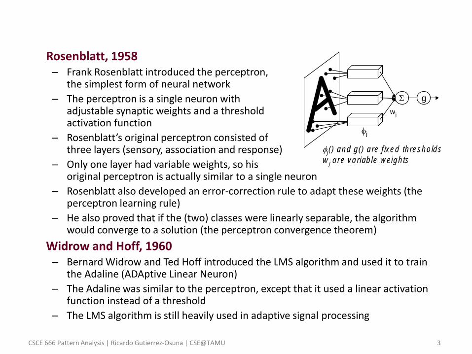
• Rosenblatt, 1958 – Frank Rosenblatt introduced the perceptron,

the simplest form of neural network

– The perceptron is a single neuron with adjustable synaptic weights and a threshold activation function

– Rosenblatt’s original perceptron consisted of three layers (sensory, association and response)

– Only one layer had variable weights, so his original perceptron is actually similar to a single neuron

– Rosenblatt also developed an error-correction rule to adapt these weights (the perceptron learning rule)

– He also proved that if the (two) classes were linearly separable, the algorithm would converge to a solution (the perceptron convergence theorem)

• Widrow and Hoff, 1960 – Bernard Widrow and Ted Hoff introduced the LMS algorithm and used it to train

the Adaline (ADAptive Linear Neuron)

– The Adaline was similar to the perceptron, except that it used a linear activation function instead of a threshold

– The LMS algorithm is still heavily used in adaptive signal processing

S g

wj

fj

fj() and g() are fixed thresholds

wj are variable weights


• Minsky and Papert, 1969 – During the 1950s and 1960s two school of thought: Artificial Intelligence and

Connectionism, competed for prestige and funding • The AI community was interested in the highest cognitive processes: logic, rational

thought and problem solving • The Connectionists’ principal model was the perceptron

– The perceptron was severely limited in that it could only learn linearly separable patterns – Connectionists struggled to find a learning algorithm for multi-layer perceptrons that

would not appear until the mid 1980s

– In their monograph “Perceptrons”, Marvin Minsky and Seymour Papert (1969) mathematically proved the limitations of Rosenblatt’s perceptron and conjectured that multi-layered perceptrons would suffer from the same limitations

– As a result of this book, research in ANNs was almost abandoned in the 1970s • Only a handful of researchers continued working on ANNs, mostly outside the US

– The 1970s saw the emergence of SOMs [van der Malsburg, 1973], [Amari, 1977], [Grossberg, 1976] and associative memories: [Kohonen, 1972], [Anderson, 1972]

The perceptron has shown itself worthy of study despite (and even because of!) its severe limitations. It has many features to attract attention: its linearity; its intriguing learning theorem; its clear paradigmatic simplicity as a kind of parallel computation. There is no reason to suppose that any of these virtues carry over to the many-layered version. Nevertheless, we consider it to be an important research problem to elucidate (or reject) our intuitive judgement that the extension to multilayer systems is sterile.


• The resurgence of the early 1980s – 1980: Steven Grossberg, one of the few researchers in the US that persevered

despite the lack of support, establishes a new principle of self-organization called Adaptive Resonance Theory (ART) in collaboration with Gail Carpenter

– 1982: John Hopfield explains the operation of a certain class of recurrent ANNs (Hopfield networks) as an associative memory using statistical mechanics. Along with backprop, Hopfield’s work was most responsible for the re-birth of ANNs

– 1982: Teuvo Kohonen presents SOMs using one- and two-dimensional lattices. Kohonen SOMs have received far more attention than van der Malsburg’s work and have become the benchmark for innovations in self-organization

– 1983: Kirkpatrick, Gelatt and Vecchi introduced Simulated Annealing for solving combinatorial optimization problems. The concept of Simulated Annealing was later used by Ackley, Hinton and Sejnowsky (1985) to develop the Boltzmann machine (the first successful realization of multi-layered ANNs)

– 1983: Barto, Sutton and Anderson popularized reinforcement learning (Interestingly, it had been considered by Minsky in his 1954 PhD dissertation)

– 1984: Valentino Braitenberg publishes his book “Vehicles” in which he advocates for a bottom-up approach to understand complex systems: start with very elementary mechanism and build up


• Rumelhart, Hinton and Williams, 1986 – In 1986, Rumelhart, Hinton and Williams announced the discovery of a

method that allowed a network to learn to discriminate between not linearly separable classes. They called the method “backward propagation of errors”, a generalization of the LMS rule

– Backprop provided the solution to the problem that had puzzled Connectionists for two decades

• Backprop was in reality a multiple invention: David Parker (1982, 1985) and Yann LeCun (1986) published similar discoveries

• However, the honor of discovering backprop goes to Paul Werbos who presented these techniques in his 1974 Ph.D. dissertation at Harvard University


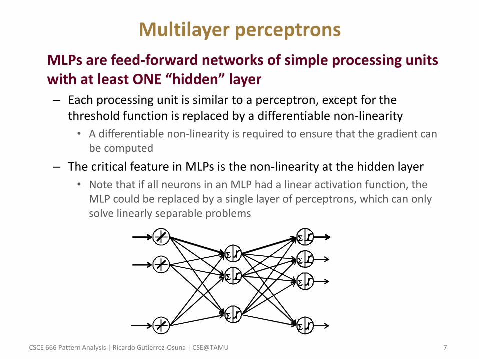
Multilayer perceptrons

• MLPs are feed-forward networks of simple processing units with at least ONE “hidden” layer – Each processing unit is similar to a perceptron, except for the

threshold function is replaced by a differentiable non-linearity

• A differentiable non-linearity is required to ensure that the gradient can be computed

– The critical feature in MLPs is the non-linearity at the hidden layer

• Note that if all neurons in an MLP had a linear activation function, the MLP could be replaced by a single layer of perceptrons, which can only solve linearly separable problems

S

S

S

S

S

S

S

SS

SS

SS

SS

SS

SS

SS


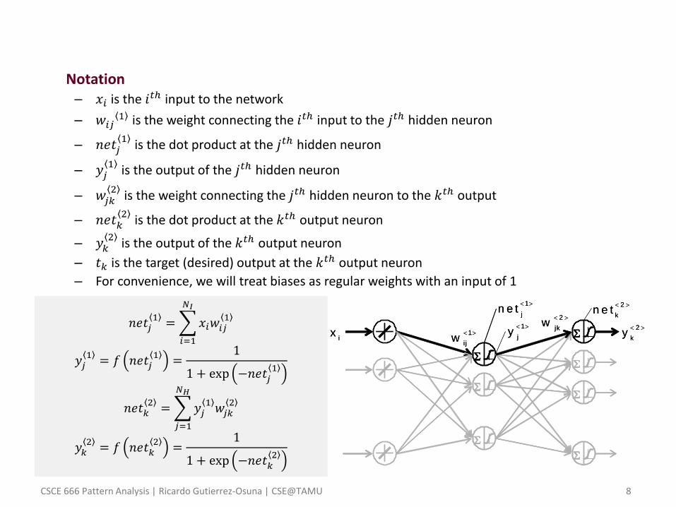
• Notation – 𝑥𝑖 is the 𝑖𝑡ℎ input to the network

– 𝑤𝑖𝑗1 is the weight connecting the 𝑖𝑡ℎ input to the 𝑗𝑡ℎ hidden neuron

– 𝑛𝑒𝑡𝑗1

is the dot product at the 𝑗𝑡ℎ hidden neuron

– 𝑦𝑗1

is the output of the 𝑗𝑡ℎ hidden neuron

– 𝑤𝑗𝑘2

is the weight connecting the 𝑗𝑡ℎ hidden neuron to the 𝑘𝑡ℎ output

– 𝑛𝑒𝑡𝑘2

is the dot product at the 𝑘𝑡ℎ output neuron

– 𝑦𝑘2

is the output of the 𝑘𝑡ℎ output neuron

– 𝑡𝑘 is the target (desired) output at the 𝑘𝑡ℎ output neuron

– For convenience, we will treat biases as regular weights with an input of 1

S

S

S

S

S

S

1

ijw

2

jkw

ix

2

kyS

2

kn e t

1

jn e t

1

jy

SS

SS

SS

SS

SS

SS

1

ijw

2

jkw

ix

2

kySS

2

kn e t

1

jn e t

1

jy

𝑛𝑒𝑡𝑗1= 𝑥𝑖𝑤𝑖𝑗

1

𝑁𝐼

𝑖=1

𝑦𝑗1

= 𝑓 𝑛𝑒𝑡𝑗1

=1

1 + exp −𝑛𝑒𝑡𝑗1

𝑛𝑒𝑡𝑘2= 𝑦𝑗

1𝑤𝑗𝑘

2

𝑁𝐻

𝑗=1

𝑦𝑘2

= 𝑓 𝑛𝑒𝑡𝑘2

=1

1 + exp −𝑛𝑒𝑡𝑘2


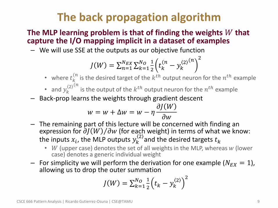
The back propagation algorithm • The MLP learning problem is that of finding the weights 𝑊 that

capture the I/O mapping implicit in a dataset of examples – We will use SSE at the outputs as our objective function

𝐽 𝑊 = 1

2𝑡𝑘(𝑛

− 𝑦𝑘2 (𝑛 2

𝑁𝑂𝑘=1

𝑁𝐸𝑋𝑛=1

• where 𝑡𝑘(𝑛

is the desired target of the 𝑘𝑡ℎ output neuron for the 𝑛𝑡ℎ example

• and 𝑦𝑘2 (𝑛

is the output of the 𝑘𝑡ℎ output neuron for the 𝑛𝑡ℎ example

– Back-prop learns the weights through gradient descent

𝑤 = 𝑤 + Δ𝑤 = 𝑤 − 𝜂𝜕𝐽 𝑊

𝜕𝑤

– The remaining part of this lecture will be concerned with finding an expression for 𝜕𝐽 𝑊 𝜕𝑤 (for each weight) in terms of what we know: the inputs 𝑥𝑖, the MLP outputs 𝑦𝑘

2 and the desired targets 𝑡𝑘 • 𝑊 (upper case) denotes the set of all weights in the MLP, whereas 𝑤 (lower

case) denotes a generic individual weight

– For simplicity we will perform the derivation for one example (𝑁𝐸𝑋 = 1), allowing us to drop the outer summation

𝐽 𝑊 = 1

2𝑡𝑘 − 𝑦𝑘

22𝑁𝑂

𝑘=1


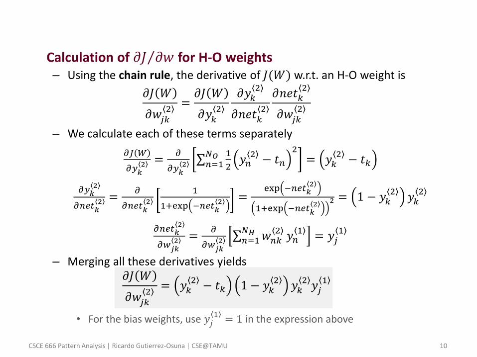
• Calculation of 𝜕𝐽 𝜕𝑤 for H-O weights – Using the chain rule, the derivative of 𝐽(𝑊) w.r.t. an H-O weight is

𝜕𝐽 𝑊

𝜕𝑤𝑗𝑘2

=𝜕𝐽 𝑊

𝜕𝑦𝑘2

𝜕𝑦𝑘2

𝜕𝑛𝑒𝑡𝑘2


𝜕𝑤𝑗𝑘2

– We calculate each of these terms separately

𝜕𝐽 𝑊

𝜕𝑦𝑘2 =

𝜕

𝜕𝑦𝑘2

1

2𝑦𝑛

2− 𝑡𝑛

2𝑁𝑂𝑛=1 = 𝑦𝑘

2− 𝑡𝑘

𝜕𝑦𝑘2

𝜕𝑛𝑒𝑡𝑘2 =

𝜕


1

1+exp −𝑛𝑒𝑡𝑘2 =

exp −𝑛𝑒𝑡𝑘2

1+exp −𝑛𝑒𝑡𝑘2 2 = 1 − 𝑦𝑘

2 𝑦𝑘2


𝜕𝑤𝑗𝑘2 =

𝜕

𝜕𝑤𝑗𝑘2 𝑤𝑛𝑘

2𝑁𝐻𝑛=1 𝑦𝑛

1 = 𝑦𝑗1

– Merging all these derivatives yields 𝜕𝐽 𝑊

𝜕𝑤𝑗𝑘2

= 𝑦𝑘2− 𝑡𝑘 1 − 𝑦𝑘

2𝑦𝑘

2𝑦𝑗

1

• For the bias weights, use 𝑦𝑗1 = 1 in the expression above


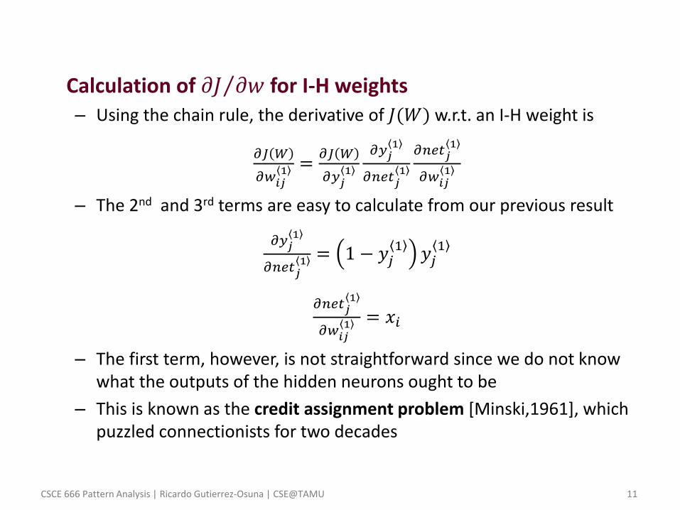
• Calculation of 𝜕𝐽 𝜕𝑤 for I-H weights – Using the chain rule, the derivative of 𝐽(𝑊) w.r.t. an I-H weight is

𝜕𝐽 𝑊

𝜕𝑤𝑖𝑗1 =

𝜕𝐽 𝑊

𝜕𝑦𝑗1

𝜕𝑦𝑗1

𝜕𝑛𝑒𝑡𝑗1


𝜕𝑤𝑖𝑗1

– The 2nd and 3rd terms are easy to calculate from our previous result

𝜕𝑦𝑗1

𝜕𝑛𝑒𝑡𝑗1 = 1 − 𝑦𝑗

1 𝑦𝑗1


𝜕𝑤𝑖𝑗1 = 𝑥𝑖

– The first term, however, is not straightforward since we do not know what the outputs of the hidden neurons ought to be

– This is known as the credit assignment problem [Minski,1961], which puzzled connectionists for two decades


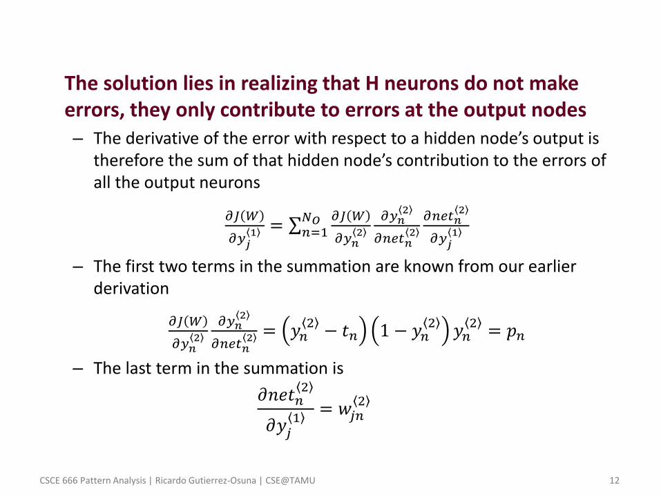
• The solution lies in realizing that H neurons do not make errors, they only contribute to errors at the output nodes – The derivative of the error with respect to a hidden node’s output is

therefore the sum of that hidden node’s contribution to the errors of all the output neurons

𝜕𝐽 𝑊

𝜕𝑦𝑗1 =

𝜕𝐽 𝑊

𝜕𝑦𝑛2

𝜕𝑦𝑛2

𝜕𝑛𝑒𝑡𝑛2


𝜕𝑦𝑗1

𝑁𝑂𝑛=1

– The first two terms in the summation are known from our earlier derivation

𝜕𝐽 𝑊

𝜕𝑦𝑛2

𝜕𝑦𝑛2

𝜕𝑛𝑒𝑡𝑛2 = 𝑦𝑛

2 − 𝑡𝑛 1 − 𝑦𝑛2 𝑦𝑛

2 = 𝑝𝑛

– The last term in the summation is


𝜕𝑦𝑗1

= 𝑤𝑗𝑛2


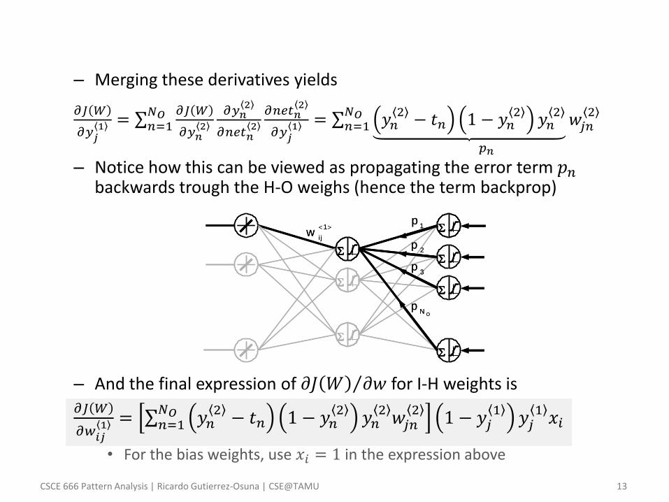
– Merging these derivatives yields

𝜕𝐽 𝑊

𝜕𝑦𝑗1 =

𝜕𝐽 𝑊

𝜕𝑦𝑛2

𝜕𝑦𝑛2



𝜕𝑦𝑗1 = 𝑦𝑛

2− 𝑡𝑛 1 − 𝑦𝑛

2𝑦𝑛

2𝑤𝑗𝑛

2

𝑝𝑛

𝑁𝑂𝑛=1

𝑁𝑂𝑛=1

– Notice how this can be viewed as propagating the error term 𝑝𝑛 backwards trough the H-O weighs (hence the term backprop)

– And the final expression of 𝜕𝐽 𝑊 𝜕𝑤 for I-H weights is 𝜕𝐽 𝑊

𝜕𝑤𝑖𝑗1 = 𝑦𝑛

2 − 𝑡𝑛 1 − 𝑦𝑛2 𝑦𝑛

2 𝑤𝑗𝑛2𝑁𝑂

𝑛=1 1 − 𝑦𝑗1 𝑦𝑗

1 𝑥𝑖

• For the bias weights, use 𝑥𝑖 = 1 in the expression above

S

S

S

S

S

S

S 1

ijw

S

S

S

2p

3p

1p

ONp

SS

SS

SS

SS

SS

SS

SS 1

ijw

SS

SS

SS

2p

3p

1p

ONp


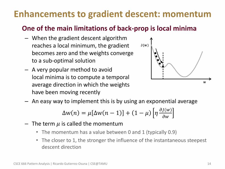
Enhancements to gradient descent: momentum

• One of the main limitations of back-prop is local minima – When the gradient descent algorithm

reaches a local minimum, the gradient becomes zero and the weights converge to a sub-optimal solution

– A very popular method to avoid local minima is to compute a temporal average direction in which the weights have been moving recently

– An easy way to implement this is by using an exponential average

Δw 𝑛 = 𝜇 Δw 𝑛 − 1 + 1 − 𝜇 𝜂𝜕𝐽(𝑤)

𝜕𝑤

– The term 𝜇 is called the momentum

• The momentum has a value between 0 and 1 (typically 0.9)

• The closer to 1, the stronger the influence of the instantaneous steepest descent direction

J (w )

w

J (w )

w


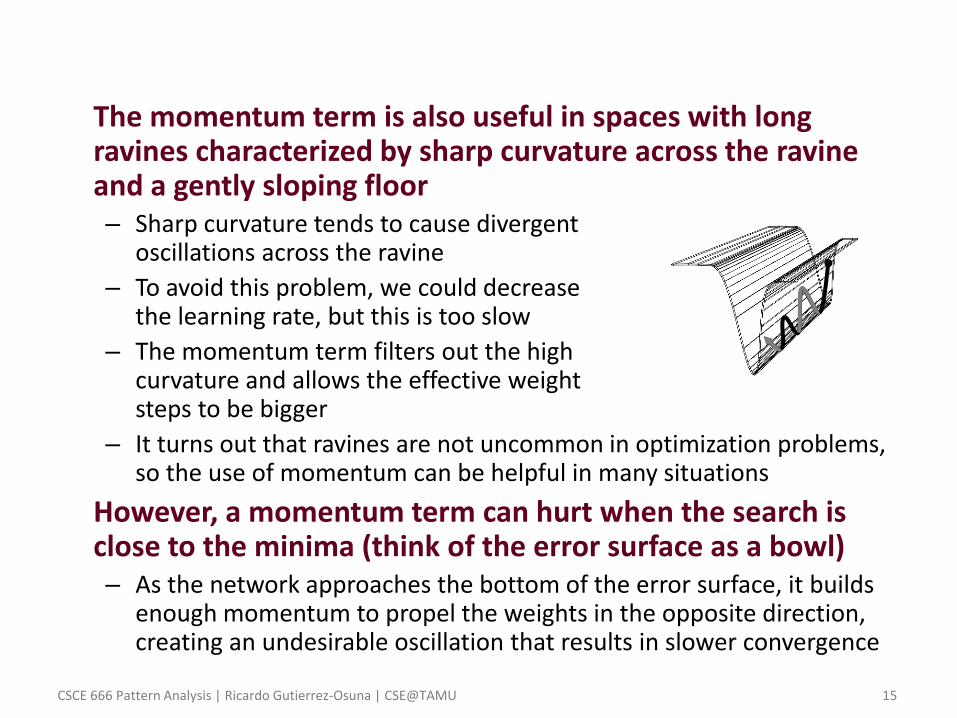
• The momentum term is also useful in spaces with long ravines characterized by sharp curvature across the ravine and a gently sloping floor – Sharp curvature tends to cause divergent

oscillations across the ravine

– To avoid this problem, we could decrease the learning rate, but this is too slow

– The momentum term filters out the high curvature and allows the effective weight steps to be bigger

– It turns out that ravines are not uncommon in optimization problems, so the use of momentum can be helpful in many situations

• However, a momentum term can hurt when the search is close to the minima (think of the error surface as a bowl) – As the network approaches the bottom of the error surface, it builds

enough momentum to propel the weights in the opposite direction, creating an undesirable oscillation that results in slower convergence


Other enhancements: adaptive learning rates

• Rather than having a unique learning rate for all weights in the MLP, let each weight to have its own learning rate – In particular, let the learning rate adapt based on the weight’s

performance during training

• If the direction in which 𝐽 𝑊 decreases w.r.t. a weight is the same as in the recent past, increase the learning rate. Otherwise decrease it.

• SOLUTION – The direction 𝛿(𝑛) in which the error decreases at time 𝑛 is given by

the sign of 𝜕𝐽 𝜕𝑤

– The direction 𝛿 (𝑛) in which the error has been decreasing “recently” is computed as the exponential average of 𝛿(𝑛)

𝛿 𝑛 + 1 = 𝜃𝛿 𝑛 + 1 − 𝜃 𝛿(𝑛)

– To determine if the current direction and the recent direction coincide we compute the product between 𝛿(𝑛) and 𝛿 (𝑛)

• If the product is greater than 0, the signs are the same

• If the product is less than 0, the signs are different


– Based on the dot product, the learning rates are adapted according to the following rule

𝜂 𝑛 = 𝜂 𝑛 − 1 + 𝜅 𝑖𝑓 𝛿 𝑛 𝛿 𝑛 > 0

𝜂 𝑛 − 1 Ψ 𝑖𝑓 𝛿 𝑛 𝛿 𝑛 ≤ 0

• 𝜅 is a constant added to the learning rate if the direction has not changed (the actual value of 𝜅 is problem dependent)

• Ψ is a fraction that is multiplied to the learning rate if the direction has changed (typically 0.5)

– Assuming also a momentum term, the final expression for the weight change becomes

Δw 𝑛 = 𝜇 Δw 𝑛 − 1 + 1 − 𝜇 𝜂 𝑛𝜕𝐽 𝑊

𝜕𝑤

• The adaptive nature of 𝜂 is made explicit by making it a function of time 𝜂(𝑛)


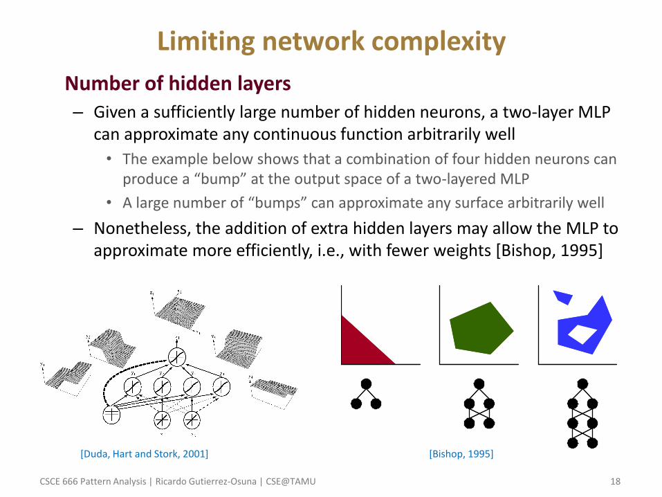
Limiting network complexity

• Number of hidden layers – Given a sufficiently large number of hidden neurons, a two-layer MLP

can approximate any continuous function arbitrarily well

• The example below shows that a combination of four hidden neurons can produce a “bump” at the output space of a two-layered MLP

• A large number of “bumps” can approximate any surface arbitrarily well

– Nonetheless, the addition of extra hidden layers may allow the MLP to approximate more efficiently, i.e., with fewer weights [Bishop, 1995]

[Duda, Hart and Stork, 2001] [Bishop, 1995]


• Number of hidden neurons – While the number of inputs and outputs are dictated by the problem, the

number of hidden units 𝑁𝐻 is not related so explicitly to the application domain • 𝑁𝐻 determines the degrees of freedom or expressive power of the model

• A small 𝑁𝐻 may not be sufficient to model complex I/O mappings

• A large 𝑁𝐻 may overfit the training data and prevent the network from generalizing to new examples

– Despite a number of “rules of thumb” published in the literature, a-priori determination of an appropriate 𝑁𝐻 is an unsolved problem • The “optimal” 𝑁𝐻 depends on multiple factors, including number of examples,

level of noise in the training set, complexity of the classification problem, number of inputs and outputs, activation functions and training algorithm.

• In practice, several MLPs are trained and evaluated in order to determine an appropriate 𝑁𝐻

– A number of adaptive approaches have also been proposed • Constructive approaches start with a small network and incrementally add

hidden neurons (e.g., cascade correlation),

• Pruning approaches, which start with a relatively large network and incrementally remove weights (e.g., optimal brain damage)


• Weight decay – To prevent the weights from growing too large (a sign of over-training)

it is convenient to add a decay term of the form 𝑤 𝑛 + 1 = 1 − 𝜖 𝑤 𝑛

• Weights that are not needed eventually decay to zero, whereas necessary weights are continuously updated by back-prop

– Weight decay is a simple form of regularization, which encourages smoother network mappings [Bishop, 1995]

• Early stopping – Early stopping can be used to prevent the MLP from over-fitting the

training set

– The stopping point may be determined by monitoring the sum-squared-error of the MLP on a validation set during training

• Training with noise (jitter) – Training with noise prevents the MLP from approximating the training

set too closely, which leads to improved generalization


Tricks of the trade • Activation function

– An MLP trained with backprop will generally train faster if the activation function is anti-symmetric: 𝑓(−𝑥) = −𝑓(𝑥) (e.g., the hyperbolic tangent)

• Target values – Obviously, it is important that the target values are within the dynamic

range of the activation function, otherwise the neuron will be unable to produce them

– In addition, it is recommended that the target values are not the asymptotic values of the activation function; otherwise backprop will tend to drive the neurons into saturation, slowing down the learning process • The slope of the activation function, which is proportional to Δ𝑤, becomes

zero at ±∞

• Input normalization – Input variables should be preprocessed so that their mean value is zero or

small compared to the variance

– Input variables should be uncorrelated (use PCA to accomplish this)

– Input variables should have the same variance (use Fukunaga’s whitening transform)


• Initial weights – Initial random weights should be small to avoid driving the neurons into

saturation • HO weights should be made larger than IH weights since they carry the back

propagated error • If the initial HO weights are very small, the weight changes at the IH layer will

initially be very small, slowing the training process

• Weight updates – The derivation of backprop was based on one training example but, in

practice, the data set contains a large number of examples – There are two basic approaches for updating the weights during training

• On-line training: weights are updated after presentation of each example • Batch training: weights are updated after presentation of all the examples (we

store the Δ𝑤 for each example, and add them up to the weight after all the examples have been presented)

– Batch training is recommended • Batch training uses the TRUE steepest descent direction • On-line training achieves lower errors earlier in training but only because the

weights are updated n (# examples) times faster than in batch mode • On-line training is sensitive to the ordering of examples

Documents

The development of artificial neural networks The back ...research.cs.tamu.edu/prism/lectures/pr/pr_l18.pdf · – In their monograph “Perceptrons”, Marvin Minsky and Seymour