1

The Developmental Testbed Center’s Final Report on the performance of the ACM2 PBL and PX surface layer model in the Air Force Weather Agency’s weather forecast

system

27 February 2015

1. Introduction The Weather Research and Forecasting (WRF) model is a mesoscale numerical weather prediction (NWP) system utilized in both research and operational forecasting applications (Skamarock et al. 2008). The model is configurable to the users’ requirements and suitable for a broad spectrum of weather regimes. The Air Force Weather Agency (AFWA) was interested in assessing a new combination of parameterizations for their operational configuration, including the Asymmetric Convective Model (ACM2) with non-local upward mixing and local downward mixing planetary boundary layer (PBL) scheme (Pleim, 2007), the Pleim-Xiu land surface model (LSM) two-layer scheme with vegetation and sub-grid tiling, and the Pleim-Xiu surface layer scheme (Xiu and Pleim 2001). To address this request, the Developmental Testbed Center (DTC) performed a rigorous test and evaluation which assessed forecast performance when substituting AFWA’s current operational PBL [Yonsei University scheme (YSU)] and land schemes (Noah LSM and Monin-Obukhov similarity) with the ACM2 and Pleim-Xiu schemes. The test was conducted in a functionally similar operational environment to AFWA; each configuration was initialized with a 6-hour “warm-start” spin up, including the Gridpoint Statistical Interpolation (GSI) component. Version 3.6.1 of the WRF model with the Advanced Research WRF (ARW) dynamic core was used. For this testing, the two configurations will be referred to as AFWAOC (when using AFWA’s current operational configuration) and ACM2PX, with AFWAOC used as the baseline. In addition to documenting the performance of the two configurations against each other, both were designated as DTC Reference Configurations (RCs), and the results have been made available to the WRF community.

2. Experiment Design For this test, the end-to-end forecast system consisted of the WRF Preprocessing System (WPS), Gridpoint Statistical Interpolation (GSI) data assimilation system, WRF, Unified Postprocessor (UPP) and the NCAR Command Language (NCL) for graphics generation. Post-processed forecasts were verified using the Model Evaluation Tools (MET). In addition, the full data set was archived and is available for dissemination to the user community upon request. The codes utilized were based on the official released versions of WPS (v3.6.1), GSI (v3.3), WRF (v3.6.1), UPP (v2.2), and MET (v5.0). Both WRF and MET included relevant bug fixes that were checked into the code repository prior to testing.

2.1 Forecast Periods Forecasts were initialized every 36 hours from 1 August 2013 through 31 August 2014, consequently creating initialization times including both 00 and 12 UTC, for a total of 264 possible cases (see Appendix A for a list of the cases). The forecasts were run out to 48 hours with output files generated every 3 hours. Due to a large gap in missing input data from mid-June through mid-July, an additional summer month (August 2013) was included to provide a more complete analysis of the summer season.

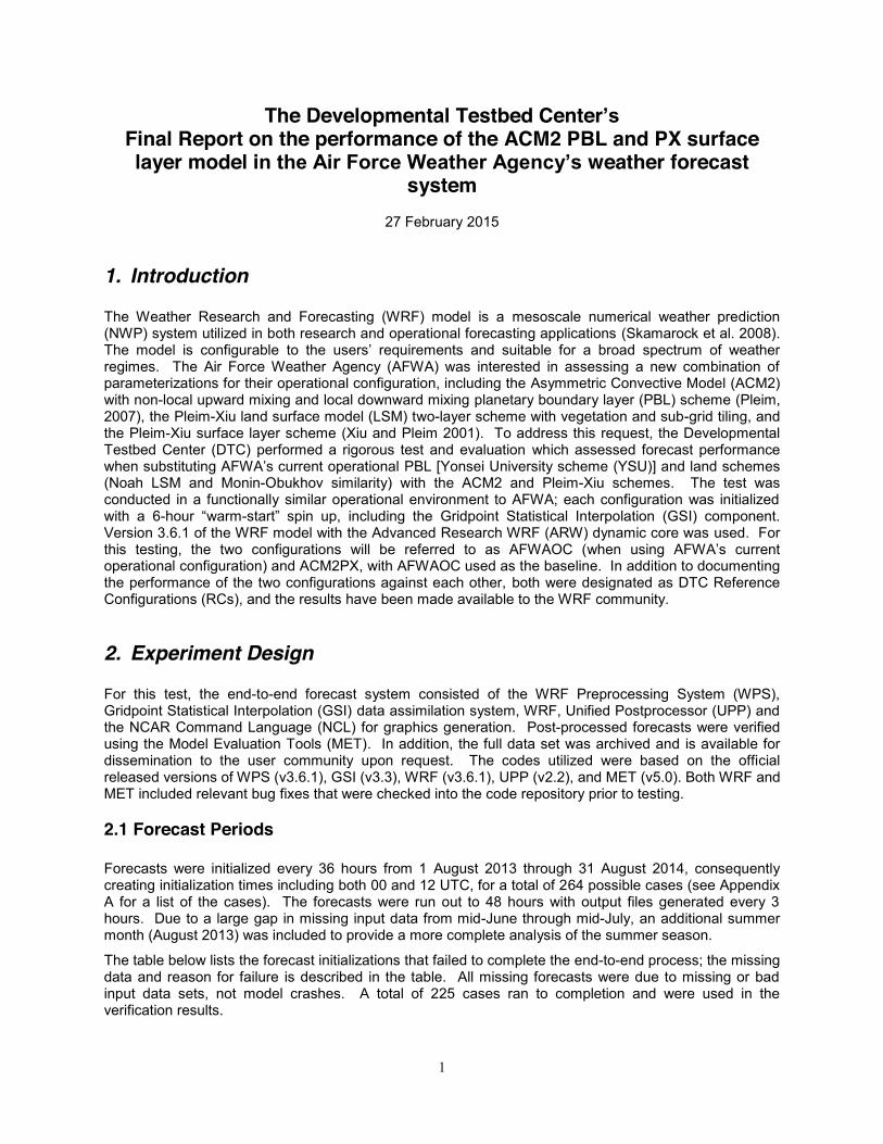
The table below lists the forecast initializations that failed to complete the end-to-end process; the missing data and reason for failure is described in the table. All missing forecasts were due to missing or bad input data sets, not model crashes. A total of 225 cases ran to completion and were used in the verification results.

2

Missing forecasts: Affected Cycle Missing data Reason 2013080112 WRF output Missing SST input data 2013080900 WRF output Missing GFS input data 2013081912 WRF output Missing GFS input data 2013082100 WRF output Missing GFS input data 2013091100 WRF output Missing obs input data 2013120400 WRF output Bad SST input data 2013122612 WRF output Missing obs input data 2013122800 WRF output Missing SST, LIS, obs input data 2013122912 WRF output Missing SST, LIS, obs input data 2013123100 WRF output Missing SST, LIS, obs input data 2014010112 WRF output Missing SST input data 2014010900 WRF output Missing SST, LIS input data 2014011012 WRF output Missing SST, LIS input data 2014012212 WRF output Bad SST input data 2014020200 WRF output Missing GFS input data 2014020312 WRF output Missing GFS input data 2014030400 WRF output Missing LIS, bad SST input data 2014031412 WRF output Missing LIS input data 2014031712 WRF output Bad SST input data 2014041800 WRF output Bad SST input data 2014061812 WRF output Missing SST, LIS, obs input data 2014062000 WRF output Missing SST, LIS, obs input data 2014062112 WRF output Missing SST, LIS, obs input data 2014062300 WRF output Missing SST, LIS, obs input data 2014062412 WRF output Missing SST, LIS, obs input data 2014062600 WRF output Missing SST, LIS, obs input data 2014062712 WRF output Missing SST, LIS, obs input data 2014062900 WRF output Missing SST, LIS, obs input data 2014063012 WRF output Missing SST, LIS, obs input data 2014070200 WRF output Missing SST, LIS, obs input data 2014070312 WRF output Missing SST, LIS, obs input data 2014070500 WRF output Missing SST, LIS, obs input data 2014070612 WRF output Missing SST, LIS, obs input data 2014070800 WRF output Missing SST, LIS, obs input data 2014070912 WRF output Missing SST, LIS, obs input data 2014071100 WRF output Missing SST, LIS, obs input data 2014071212 WRF output Missing SST, LIS, obs input data 2014071400 WRF output Missing SST, LIS, obs input data 2014071512 WRF output Missing SST, LIS, obs input data

2.2 Initial and Boundary Conditions Initial conditions (ICs) and lateral boundary conditions (LBCs) were derived from the 0.5° x 0.5° Global Forecast System (GFS). Output from AFWA’s land information system (LIS) running with the Noah land surface model version 2.7.1 was used to initialize the lower boundary conditions (LoBCs); the files used for initializing the LoBCs were generated by AFWA and then provided to the DTC for the testing period. In addition, a daily, real-time sea surface temperature (SST) product from Fleet Numerical Meteorology and Oceanography Center (FNMOC) was used to initialize the (SST) field for the forecasts.

3

The time-invariant components of the LoBCs (topography, soil, vegetation type, etc.) were derived from United States Geological Survey (USGS) input data and were generated through the geogrid program of WPS. The avg_tsfc program of WPS was also used to compute the mean surface air temperature in order to provide improved water temperature initialization for lakes and smaller bodies of water in the domain that are further away from an ocean. A 6-hour “warm start” spin-up procedure (Fig. 1) preceded each forecast. Data assimilation using GSI was conducted at the beginning and end of the 6-hour window using observation data files provided by AFWA. At the beginning of the data assimilation window, the GFS-derived initial conditions were used as the model background, and at the end of the window, the 6-hour WRF forecasts initialized by the GSI analysis were used. The default files of model error covariance and observation error from NAM were used in GSI. After each GSI job, the LBCs initially derived from GFS were updated and used in the subsequent forecasts. For the GSI system to effectively assimilate satellite radiance observations, appropriate bias correction is crucial. In operational systems, the bias correction files are usually trained in a cycling fashion. In the present test, training the files in continuous cycling was not feasible because forecasts were initialized every 36 hours. Therefore, the GFS-trained satellite bias correction files at the corresponding time were used. In each “warm-start”, the GFS satellite bias correction files were applied at the beginning of the 6-hour data assimilation window, and the updated bias files from this GSI job were then used for correcting bias at the end of the window.

2.3 Model Configuration Specifics 2.3.1 Domain Configuration A 15-km contiguous U.S. (CONUS) grid was employed for this test. The domain (Fig. 2) was selected such that it covers complex terrain, plains, and coastal regions from the Gulf of Mexico, spanning north to Central Canada in order to capture diverse regional effects for worldwide comparability. The domain was 403 x 302 gridpoints, for a total of 121,706 gridpoints. The Lambert-Conformal map projection was used and the model was configured to have 56 vertical levels (57 sigma entries) with the model top at 10 hPa.

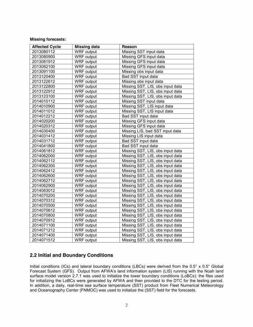
2.3.2 Model Configuration The table below lists AFWA’s current operational configuration and the ACM2PX replacement configuration that were used in this testing.

Both configurations were run with a long time step of 90 s and an acoustic time step of 4 s. Calls to the boundary layer and microphysics were performed every time step, whereas the cumulus parameterization was called every 5 minutes and radiation every 30 minutes.

Current AFWAOC ACM2PX Replacement Config

Microphysics WRF Single-Moment 5 Scheme (opt 4)

WRF Single-Moment 5 Scheme (opt 4)

Radiation LW and SW New Rapid Radiative Transfer Model (opt 4)

New Rapid Radiative Transfer Model (opt 4)

Surface Layer Monin-Obukhov Similarity Theory (opt 91)

Pleim Xiu (opt 7)

Land-Surface Model Noah (opt 2) Pleim Xiu (opt 7)

Planetary Boundary Layer Yonsei University Scheme (opt 1) Asymmetric Convective Model 2 (opt 7)

Convection Kain-Fritsch Scheme (opt 1) Kain-Fritsch Scheme (opt 1)

4

The ARW solver offers a number of run-time options for the numerics, as well as various filter and damping options (Skamarock et al. 2008). The ARW was configured to use the following numeric options: 3rd-order Runge-Kutta time integration, 5th-order horizontal momentum and scalar advection, and 3rd-order vertical momentum and scalar advection. In addition, the following filter/damping options were utilized: three-dimensional divergence damping (coefficient 0.1), external mode filter (coefficient 0.01), off-center integration of vertical momentum and geopotential equations (coefficient 0.5), vertical-velocity damping, and a 5-km-deep diffusive damping layer at the top of the domain (coefficient 0.05). Positive-definite moisture advection was also turned on. Appendix B provides relevant portions of the namelist.input file.

2.4 Post-processing The unipost program within UPP was used to destagger the forecasts, generate derived meteorological variables, and vertically interpolate fields to isobaric levels. The post-processed files included two- and three-dimensional fields on constant pressure levels, both of which were required by the plotting and verification programs. Three-dimensional post-processed fields on model native vertical coordinates were also output and used to generate graphical forecast sounding plots.

3. Computational Efficiency For the 225 initializations that ran to completion, the central processing unit (CPU) time required to run WRF for the two configurations was calculated to assess the increase in computational demands when running the two differing configurations. This testing effort was conducted on an IBM system, and each model initialization was run on 512 processors. Overall, a consistent difference in computational run time between the AFWAOC and the ACM2PX configurations were noted, indicating the ACM2PX configuration, on average, takes 5.9% longer to run to completion.

4. Model Verification The MET package was used to generate objective model verification. MET is comprised of grid-to-point verification, which was utilized to compare gridded surface and upper-air model data to point observations, as well as grid-to-grid verification, which was utilized to verify Quantitative Precipitation Forecast (QPF). An additional type of grid-to-grid verification was also performed for this test using the series-analysis tool in MET which accumulates a metric of choices on a grid-by-grid basis over a specified time period and can be used to quantify how model performance varies over a domain. This tool can be used to identify regional differences within a single configuration as well as to highlight differences between the two configurations. While traditional line series plots provide an overall statistic for a region, investigating metrics on a grid-by-grid basis can offer insight as to where the configuration is or is not performing well, which can give beneficial information to both forecasters and model developers. Verification statistics generated by MET for each retrospective case were loaded into a MySQL database. Data was then retrieved from this database to compute and plot specified aggregated statistics using routines developed by the DTC in the statistical programming language, R. Several domains were verified for the surface and upper air, as well as precipitation variables. Area-averaged results were computed for the CONUS domain, East and West regions, and 14 sub-regions (Fig. 3). While only a portion of the full results will be discussed in detail for this report, all East, West, and sub-domain results are available on the DTC webpage established for this particular testing and evaluation activity (http://www.dtcenter.org/eval/meso_mod/afwa_test/wrf_v3.6.1/index.php). In addition

5

to the regional stratification, the verification statistics were also stratified by vertical level and lead time for the 00 UTC and 12 UTC initialization hours combined, and by forecast lead time and precipitation threshold for 00 UTC and 12 UTC initialized forecasts individually for surface fields in order to preserve the diurnal signal. Each type of verification metric is accompanied by confidence intervals (CIs), at the 99% level, computed using the appropriate statistical method. Both configurations were run for the same cases allowing for a pair-wise difference methodology to be applied, as appropriate. The CIs on the pair-wise differences between statistics for the two configurations objectively determine whether the differences are statistically significant (SS); if the CIs on the pair-wise difference statistics include zero, the differences are not SS. Due to the nonlinear attributes of frequency bias, it is not amenable to a pair-wise difference comparison. Therefore, the more powerful method to establish SS could not be used and, thus, a more conservative estimate of SS was employed based solely on whether the aggregate statistics, with the accompanying CIs, overlapped between the two configurations. If no overlap was noted for a particular threshold, the differences between the two configurations were considered SS. Due to the large number of cases used in this test, many SS pair-wise differences were anticipated. ln many cases, the magnitude of the SS differences was quite small and did not yield practically meaningful results. Therefore, in addition to determining SS, the concept of establishing practical significance (PS) was also utilized in this test. PS was determined by filtering results to highlight pair-wise differences greater than the operational measurement uncertainty requirements and instrument performance as specified by the World Meteorological Organization (WMO; http://www.wmo.int/pages/prog/gcos/documents/gruanmanuals/CIMO/CIMO_Guide-7th_Edition-2008.pdf). To establish PS between the two configurations, the following criteria were applied: temperature and dew point temperature differences greater than 0.1 K and wind speed differences greater than 0.5 m s-1. PS was not considered for metrics used in precipitation verification [i.e., Gilbert Skill Score (GSS) or frequency bias] because those metrics are calculated via a contingency table, which is based on counts of yes and no forecasts.

4.1 Temperature, Dew Point Temperature, and Winds Forecasts of surface and upper air temperature, dew point temperature, and wind were bilinearly interpolated to the location of the observations (METARs and RAOBS) within the National Centers for Environmental Prediction (NCEP) North American Data Assimilation System (NDAS) prepbufr files. Objective model verification statistics were then generated for surface (using METARs) and upper air (using RAOBS) temperature, dew point temperature, and wind. Because shelter-level variables are not available in the model at the initial time, surface verification results start at the 3-hour lead time and go out 48 hours by 3-hour increments. For upper air, verification statistics were computed at the mandatory levels using radiosonde observations and computed at 12-hour intervals out to 48 hours. Because of known errors associated with radiosonde moisture measurements at high altitudes, the analysis of the upper air dew point temperature verification focuses on levels at and below 500 hPa. Bias and bias-corrected root-mean-square-error (BCRMSE) were computed separately for surface and upper air observations. The CIs were computed from the standard error estimates about the median value of the stratified results using a parametric method and a correction for first-order autocorrelation.

4.2 Precipitation For the QPF verification, a grid-to-grid comparison was made by first using the budget method to interpolate the precipitation analyses to the 15-km model integration domain, which conserves the total area-average precipitation amounts. This regridded analysis was then used to evaluate the forecast. Accumulation periods of 3 and 24 hours were examined. NCEP’s Climatology-Calibrated Precipitation Analysis (CCPA) was used as the observational dataset for both the 3- and 24-hour accumulations. Traditionally 24-h QPF verification is performed at times valid at 12 UTC; therefore, the 24-hour QPFs were examined for the 24- and 48-hour lead times for the 12 UTC initializations and 36-hour lead time for

6

the 00 UTC initializations. Traditional verification metrics computed, included the GSS and frequency bias. For the precipitation statistics, a bootstrapping CI method was applied.

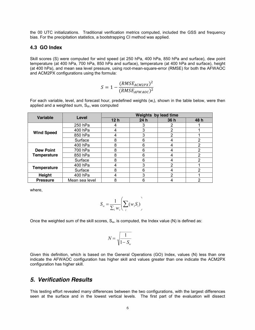
4.3 GO Index Skill scores (S) were computed for wind speed (at 250 hPa, 400 hPa, 850 hPa and surface), dew point temperature (at 400 hPa, 700 hPa, 850 hPa and surface), temperature (at 400 hPa and surface), height (at 400 hPa), and mean sea level pressure, using root-mean-square-error (RMSE) for both the AFWAOC and ACM2PX configurations using the formula:

𝑆 = 1 − (𝑅𝑀𝑆𝐸𝐴𝐶𝑀2𝑃𝑋)2

(𝑅𝑀𝑆𝐸𝐴𝐹𝑊𝐴𝑂𝐶)2 For each variable, level, and forecast hour, predefined weights (wi), shown in the table below, were then applied and a weighted sum, SW, was computed

Variable Level Weights by lead time 12 h 24 h 36 h 48 h

Wind Speed 250 hPa 4 3 2 1 400 hPa 4 3 2 1 850 hPa 4 3 2 1 Surface 8 6 4 2

Dew Point Temperature

400 hPa 8 6 4 2 700 hPa 8 6 4 2 850 hPa 8 6 4 2 Surface 8 6 4 2

Temperature 400 hPa 4 3 2 1 Surface 8 6 4 2

Height 400 hPa 4 3 2 1 Pressure Mean sea level 8 6 4 2

where, Once the weighted sum of the skill scores, Sw, is computed, the Index value (N) is defined as: Given this definition, which is based on the General Operations (GO) Index, values (N) less than one indicate the AFWAOC configuration has higher skill and values greater than one indicate the ACM2PX configuration has higher skill.

5. Verification Results This testing effort revealed many differences between the two configurations, with the largest differences seen at the surface and in the lowest vertical levels. The first part of the evaluation will dissect

��

Sw 1

¦i wi(wiSi

i¦ )§�

©�¨�

·�

¹�¸�

��

N 1

1� Sw

7

configuration performance over the CONUS for all temporal aggregations for the standard verification metrics. In addition to the time series plots provided, further investigation of forecast performance for both configurations over diverse regions of the CONUS is included. The bias at each observation station is presented by surface variable to provide a means to spatially assess the configurations performance respective to the observations. When visualizing the results in this manner, seasonal differences are apparent, both regionally and between configurations. On a similar note, precipitation verification scores will also be visualized by accumulating metrics on a grid-by-grid basis over a specified time period to quantify configuration performance over the domain. Differences between the two configurations are computed by subtracting ACM2PX from AFWAOC. Since BCRMSE is always a positive quantity with a perfect score of zero, this results in positive (negative) differences indicating the ACM2PX (AFWAOC) configuration has a lower BCRMSE and is favored. Bias also has a perfect score of zero but can have positive or negative values; therefore, when examining pair-wise differences, it is important to note the magnitude of the bias in relation to the perfect score for each individual configuration to know which has a smaller bias and is, thus, favored. For GSS, the perfect score is one, and the no-skill forecast is zero and below with a lower limit of -1/3. Thus, if the pair-wise difference is positive (negative), the AFWAOC (ACM2PX) configuration has a higher GSS and is favored. Frequency bias has a perfect score of one, but as described earlier, SS is determined by the overlap of CIs attached to the aggregate value. A breakdown of the configurations with SS and PS better performance by variable, season, statistic, level, threshold, initialization hour, and forecast lead time aggregated over the CONUS domain is summarized in Tables 1-8, where the favored configuration is highlighted.

5.1 CONUS Upper Air Analysis 5.1.1 Temperature BCRMSE and bias Regardless of temporal aggregation or forecast lead time, both configurations have a minimum in temperature BCRMSE values between 500 and 300 hPa, with the largest error occurring at the lower and upper-levels (Fig. 4). In general, the largest differences between the two configurations are seen at 850 and 700 hPa; PS pair-wise differences only occur at 700 hPa or below (see Table 1), with most PS pair-wise differences occurring in the winter and spring and showing ACM2PX as being more skilled. In addition, there are a number of SS pair-wise differences, with most favoring ACM2PX in the middle-to-upper levels. An exception is noted in the summer aggregation, where AFWAOC is favored in low-to-middle levels, with one difference being PS. The shape of the temperature bias distribution is highly dependent on temporal aggregation, vertical level, and forecast lead time (e.g., Fig. 5). A consistent pattern among them, however, is that PS pair-wise differences between the two configurations are typically seen most frequently at 850 and 700 hPa, and differences generally grow with forecast lead time. In the summer aggregation at 850 hPa, ACM2PX has a neutral bias transitioning to a small warm bias with forecast lead time; meanwhile AFWAOC has a small warm bias that grows with forecast lead time. Between 850 hPa and 700 hPa, there is a sharp increase in bias for ACM2PX, while AFWAOC’s bias only has a smaller slope of increase before both configurations have a decrease in bias and transition to a more neutral bias by 300 hPa. In winter, at the 12-h forecast lead time, both configurations have similar cold biases; however, by the 48-h forecast, AFWAOC has a stronger cold bias than ACM2PX that extends up to 700 hPa. The SS/PS pair-wise differences are a reflection of the temperature bias distributions varying between seasons and vertical level (see Table 1). A majority of the PS differences show ACM2PX as the better performing configuration, with the strongest signals occurring in the lowest levels (i.e., 850 and 700 hPa), upper levels (i.e., 300 – 150 hPa) and/or at longer forecast lead times. Exceptions are noted in the fall and spring aggregations with AFWAOC being closer to the observations at 850 hPa at most forecast lead times.

8

5.1.2 Dew Point Temperature BCRMSE and bias An increase in dew point temperature BCRMSE is noted as forecast lead time increases and pressure decreases for both configurations and all temporal aggregations (Fig. 6), with exception of the winter aggregation, where at most forecast lead times, a slight decrease in median BCRMSE from 700 hPa to 500 hPa is observed. A number of PS pair-wise differences are seen in Table 2, with all but one difference favoring AFWAOC. The largest number of PS pair-wise differences are noted for the summer aggregation where a majority of levels and forecast lead times indicate AFWAOC is the better performer. A smaller number of PS pair-wise differences favoring the AFWAOC are also seen for the annual and fall aggregations; however, only one lead time and level is PS during either the winter or spring aggregations. In general, regardless of temporal aggregation or forecast lead time, both configurations have higher moisture biases at 500 hPa as compared to 850 hPa (Fig. 7). In the annual aggregation, with exception to the 48-h forecast lead time at 850 hPa, both configurations have a moist bias at all vertical levels for all forecast lead times, with ACM2PX having forecasts closer to the observations than AFWAOC at 700 and 500 hPa. Spring and winter aggregations are similar in that there are minimal differences between the two configurations, and with exception to several forecast lead times where there are unbiased forecasts at 850 hPa in the winter, there is a moist bias at all vertical levels for all forecast lead times. In summer, ACM2PX is typically moister at 850 hPa than AFWAOC, which has a neutral bias at all forecast lead times; ACM2PX transitions to a neutral bias at 700 hPa (i.e., decreasing bias with pressure). In fall, ACM2PX typically has smaller median bias values than AFWAOC at all forecast lead times and vertical levels. As highlighted above, there are a number of pair-wise differences with all but one PS, with a majority showing better performance in ACM2PX for the annual, summer, and fall aggregations (see Table 2). Most of the differences favoring ACM2PX are at 700 and 500 hPa, spanning multiple forecast lead times. Superior performance by AFWAOC is noted in the summer aggregation at all forecast lead times at 850 hPa. 5.1.3 Wind Speed BCRMSE and bias For both configurations, wind speed BCRMSE generally increases from a minimum in the lowest levels to a maximum around 300–200 hPa, with decreasing error further aloft (Fig. 8). As forecast lead time increases, the errors also show a tendency to increase. Overall, both configurations have very similar distributions of BCRMSE; this is reflected when examining the statistical significance, where only a few scattered SS pair-wise differences are noted and none being PS (see Table 3). Overall, most differences show ACM2PX as the better performer and are generally in the annual, winter, and spring aggregations with a concentration of differences at 850 hPa. Overall, for all seasonal aggregations at the 12-h forecast lead time, a neutral-to-low wind speed bias is noted at 850 hPa, which transitions to a low bias up to 200 hPa (Fig. 9). As forecast lead time increases, a shift to higher wind speed bias is seen at 850 hPa. In general, AFWAOC has higher median biases than ACM2PX in the lower-to-middle levels. Regardless of temporal aggregation or forecast lead time, a sharp increase in wind speed bias is noted from 200 hPa to 100 hPa While there are a number of SS pair-wise differences, only one is PS. In general, there is a split in the better performing configuration, with AFWAOC having lower errors in the annual, summer, and spring aggregations between 700 – 400 hPa and ACM2PX performing better in annual winter, fall, and spring aggregations at 850 hPa and at 300 hPa and above (see Table 3).

5.2 CONUS Surface Analysis 5.2.1 Temperature BCRMSE and Bias For both configurations, a diurnal trend with a general increase in 2 m temperature BCRMSE is seen for all aggregations over the CONUS for both the 00 and 12 UTC initializations (Fig. 10). The weakest diurnal signal is observed in the annual aggregation for both configurations. A number of SS and PS pair-wise differences are noted, with most being PS and occurring in the mid-to-later portion of the forecast

9

period (Table 4). The fewest number of PS pair-wise differences tend to occur during the winter and fall aggregations. Nearly all of the pair-wise differences favor ACM2PX, regardless of initialization or seasonal aggregation. When considering 2 m temperature bias, both AFWAOC and ACM2PX have a diurnal signal, regardless of initialization time or temporal aggregation (Fig. 11); however, a phase shift is noted between the two configurations and the amplitude is generally smaller for ACM2PX. For AFWAOC, a SS cold bias is noted for a majority of forecast hours. Exceptions include occasional unbiased forecasts near 15 UTC for several temporal aggregations and SS warm biases during the daytime hours for the summer aggregation. For the winter aggregation, the largest cold bias is noted around 00 UTC, while for all other temporal aggregations the largest cold bias is noted during the overnight hours between 00 - 12 UTC. For ACM2PX, the error distribution depends strongly on the temporal aggregation; for the annual, and fall aggregations the maximum error is a cold bias seen during the daytime hours, the spring and winter aggregations have the largest (cold) bias at valid times from 03 – 09 UTC, and for the summer aggregation the maximum error is a warm bias noted around 09 – 12 UTC valid times. Typically, ACM2PX is warmer than AFWAOC during the overnight hours and colder during the daytime, except for the spring aggregation where ACM2PX is always warmer and the winter aggregation where AFWAOC is warmer except during 21 – 00 UTC. All differences for 2 m temperature bias are PS, with a weak diurnal signal in which configuration is favored (Table 4). For times valid between 00 – 09 UTC, ACM2PX is generally the better performer; for valid times between 12 – 21 UTC, AFWAOC is favored more often during the summer and fall aggregations, while ACM2PX is favored more often during the winter and spring aggregations. There is a dependence on initialization and seasonal aggregation. As mentioned above, there is a clear diurnal signature in mean error (bias) for all temporal aggregations at both the 00 and 12 UTC initializations. As an example, in the summer aggregation a pronounced peak in warm bias was observed at 12 and 15 UTC for a majority of the sub-regions of the ACM2PX and AFWAOC configurations, respectively. The timing of the peak cold bias had larger variability, but for many regions it was observed between 21 to 09 UTC. Figure 12(a-d) is used to illustrate the bias of the 2 m temperature for the two configurations during the times of peak warm bias. For the summer aggregation, both the 36 and 39 hour forecast lead times of the 00 UTC initializations (valid 12 and 15 UTC, respectively) are shown. For the ACM2PX diurnal maximum at the 36 hour lead time (Fig. 12b), a warm bias is observed from the Great Basin (GRB) extending eastward across to the western half of the Midwest (MDW), Lower Mississippi Valley (LMV) and Gulf of Mexico Coast (GMC). Cold biases are generally confined within the Southwest Desert (SWD) and eastern MDW regions. At this same forecast hour, the AFWAOC has a larger cold bias, particularly in the MDW, LMV and GMC as well as along the West Coast (Fig. 12a). A smaller warm or even cold bias is observed over the plains and Northern and Southern Rocky Mountain regions (NMT and SMT) where the ACM2PX exhibited large warm biases. However, there is a noted 3-hour phase difference in the diurnal signal when comparing both configurations, with AFWAOC peaking, instead, at forecast hour 39. Therefore, a more suited comparison of the diurnal maximums in bias may be the 36-hour ACM2PX forecast with the 39-hour AFWAOC forecast (Fig. 12c) which appear more similar in pattern. Differences are noted across northern MDW and along the eastern edge of the Northeastern Coast (NEC), where the bias is colder in the AFWAOC, as well as the over the Southwest Coast (SWC) where AFWAOC exhibits a warmer bias. The 39-hour forecast for ACM2PX (Fig. 12d) shows a general change to lower bias values across much of the CONUS resulting in ACM2PX being colder than the AFWAOC at the same forecast hour. At forecast hour 45 (valid at 21 UTC), large differences are observed mainly across the Eastern CONUS where AFWAOC (Fig. 12e) is warmer than ACM2PX (Fig. 12f). For the fall temperature bias for the 00 UTC initialization at forecast hour 45 (Fig. 13), both configurations show a general cold bias across nearly the entire CONUS with warm biases present along the western coast. In western MDW a near-zero mean bias for AFWAOC is preferred over the colder ACM2PX. ACM2PX is also notably colder in the state of Texas. On the other hand, AFWAOC sees a colder bias compared to ACM2PX in GRB and northern NEC. For the winter aggregation, a strong cold bias is evident in both configurations at forecast hour 36 for the 00 UTC initialization, where only a few regions exhibit a warm bias (Fig 14). Warm biases are especially

10

prominent in the Southern Plains (SPL) and SWC, while cold biases dominate most other regions. The general spatial patterns of the biases between the two configurations are similar. As stated previously, the configuration performing better depends on the valid time. Specifically, at forecast hour 36, AFWAOC has an overall smaller cold bias [mainly over MDW, the Appalachian Mountains (APL), and LMV] while the opposite is true at forecast hour 45 (with the largest differences across the West). In the spring, when there are significant differences between the two configurations, ACM2PX is more often favored over AFWAOC for both initializations. Figure 15 provides evidence of this for the 45-hour forecast lead time which shows large cold biases over NMT, SMT, GRB, SWD, Southeast Coast (SEC), NEC and northern MDW for AFWAOC while ACM2PX has a smaller cold or even warm bias that is closer to the observations across many of those regions. On the other hand, ACM2PX has a large warm bias over much of the Northern Plains (NPL), SPL, MDW, and LMV and AFWAOC is generally closer to the observations with a near-neutral bias in these regions at this time. 5.2.2 Dew Point Temperature BCRMSE and Bias Similar to 2 m temperature, a diurnal signal superimposed within a gentle increase in errors with time is present in 2 m dew point temperature BCRMSE for all temporal aggregations, both initializations, and both configurations (Fig. 16). A slightly amplified diurnal signal with larger errors around times valid 21 – 03 UTC is noted for ACM2PX. PS pair-wise differences are generally noted between the 18 – 06 UTC valid times and mostly favor the AFWAOC (Table 5). The fewest PS pair-wise differences are noted for the winter aggregation and the most in the spring aggregation. For all temporal aggregations and both initializations, a prominent diurnal signal in 2 m dew point temperature bias is noted, with a peak in the dew point temperature bias signal between valid times of 18 – 03 UTC and a minimum in the signal between 09 – 15 UTC (Fig. 17). In the annual, summer, and spring aggregations, ACM2PX is SS higher than AFWAOC and has a wet bias at most forecast lead times, with exception to occasional lead times valid around 09 – 18 UTC, where there is an unbiased forecast. The two configurations have the largest divergence in bias values in the overnight into morning hours (i.e., valid 03 – 12 UTC); this pattern is observed in all but the winter aggregation. Typically at these valid times ACM2PX has higher magnitude values than AFWAOC with the favored configuration dependent on temporal aggregation (Table 5). In contrast, for the winter aggregation during the 24-48 hour forecast lead times, ACM2PX has lower median values than AFWAOC leading to more frequent unbiased or dry bias forecasts. It should be noted, however, in the winter aggregation both configurations have larger CIs attached to the median bias values. When pair-wise differences are noted, all are PS, with the least amount of differences occurring in the winter and spring temporal aggregations, which is likely due to the larger CIs mentioned above. More PS differences favor AFWAOC; however, there are PS pair-wise differences that favor ACM2PX, especially during the fall at times valid 09 – 15 UTC and the winter and spring for the 12 UTC initializations. As seen in the time series analysis, the ACM2PX has a large moist bias across much of the CONUS at all lead times during the summer, especially those valid at 00 UTC. On the other hand, a dry bias is commonly observed in AFWAOC for many regions, with the exception of MDW during the period 15 – 00 UTC and much of the eastern CONUS at 00 UTC valid times (not shown). The 36-hour AFWAOC forecast initialized at 00 UTC (Fig. 18a) shows the dry bias across much of the CONUS; moist biases are generally observed only along the coast lines. While most regions of ACM2PX (Fig. 18b) exhibit a moist bias, the strongest biases are along the west coast, especially SWC. The 45-hour forecast shows a strong moistening of the MDW and northern NEC in AFWAOC (Fig. 18c) while nearly all regions of ACM2PX have an increase in the moist bias (Fig. 18d). Small dry pockets are observed in the state of Oklahoma and along the APL/SEC border. For the fall aggregation, the ACM2PX sees an overall drier bias as compared to the summer aggregation resulting in smaller dew point temperature bias differences between the two configurations. At the 45-hour forecast lead time (Fig. 19), differences are observed in the eastern CONUS. In APL and eastern MDW and LMV, ACM2PX exhibits a dry bias compared to near-neutral bias values in AFWAOC.

11

Differences such as a cold bias in AFWAOC compared to a warm or neutral bias for ACM2PX, are also noted over the plains regions. For most lead times, the biggest difference between the two configurations is in SWC, which exhibits a large moist bias for ACM2PX and a dry bias for AFWAOC. Unlike with the other temporal aggregations thus far, for the winter season, there is a more prevalent dry bias for ACM2PX, especially over the eastern CONUS. At the 36-hour forecast lead time, this is apparent in the LMV, GMC, and MDW regions (Fig. 20). While AFWAOC also indicates a dry bias over much of the eastern CONUS, the magnitude is smaller making it the better performer. On the other hand, ACM2PX preforms better over most of the west. For the 45-hour forecast, both configurations have a moist bias across the west and ACM2PX is generally the preferred configuration. While AFWAOC has an east/west gradient of dry and moist bias pattern across the eastern portion of the CONUS, ACM2PX has a more north/south gradient. The eastern CONUS generally favors the AFWAOC configuration, except in NEC where AFWAOC is more moist. While the spring aggregation generally exhibits more frequent neutral to moist biases, the 45-hour forecast does exhibit dry biases in some regions, most notably in ACM2PX (Fig. 21). Overall, the eastern CONUS generally exhibits a moist bias in AFWAOC while ACM2PX has dry biases in LMV, APL, and southwest MDW. In the West, while AFWAOC generally has a moist bias with exception to SWC, ACM2PX more often exhibits a dry bias with exception to SWD and portions of SMT and SPL. 5.2.3 Wind BCRMSE and Bias For 10 m wind speed BCRMSE, both configurations display a weak diurnal signal with a general increase with forecast lead time for most temporal aggregations and both initialization times (Fig. 22); no diurnal trend is present in the winter aggregation. The errors are largest at times valid between 21 – 03 UTC, while the smallest errors are seen at times valid near 12 UTC. No PS pair-wise differences are seen (Table 6); however, a large number of SS pair-wise differences are noted. A majority of the SS pair-wise differences favor the ACM2PX, with the only exception noted between 18 – 03 UTC valid times for the summer aggregation, which favor AFWAOC. The fewest number of SS pair-wise differences occur during the fall and spring aggregations, while all forecast lead times show SS differences favoring ACM2PX for the winter aggregation. A prominent diurnal signal in bias is seen for all temporal aggregations and both initializations for 10 m wind speed bias, with the highest errors seen at times valid 06 – 12 UTC and with lowest errors at times valid 18 – 00 UTC (Fig. 23). With only a few exceptions during the spring and summer aggregations for the 12 UTC initializations, a high wind speed bias is observed regardless of initialization and temporal aggregation. While a number of SS pair-wise differences are observed, none are PS (Table 6). AFWAOC is the better performer for all times that indicate a SS pair-wise difference for the summer and fall aggregations and for most of the spring aggregation valid times (exception: 03 UTC, where ACM2PX is favored). For the winter aggregation, the signal indicates that ACM2PX is the better performer for all times with SS pair-wise differences except at the valid time of 18 UTC, which favors AFWAOC. While there are many statistically significant differences between the two configurations, the spatial differences of wind speed bias are small across the CONUS. Figure 24 illustrates the wind speed bias by observation station using the 36- and 45-hour forecast lead times for the summer aggregation. As mentioned in the lead series discussion, AFWAOC generally has a statistically significant better forecast for most lead hours. At forecast hour 36 for the 00 UTC initializations during the summer aggregation (Fig. 24a,b; valid 12 UTC), a high speed bias is observed over most of the CONUS for both initializations. At the 45-hour forecast lead time (Fig 24c,d; valid 21 UTC), the wind speed bias is lower over much of the CONUS for both configurations. A general low speed bias is noted over the West, while a high bias is still present over much of the East. ACM2PX is closer to the observations over the plains where AFWAOC is too low; however, AFWAOC is closer to the observations across the East with a smaller high bias compared to ACM2PX. In SWC, ACM2PX has a larger low speed bias, and AFWAOC is preferred.

12

Opposite from the other temporal aggregations for wind speed bias, during the winter aggregation ACM2PX generally has better forecast performance than AFWAOC. Looking at the 36-hour forecast spatially (Fig. 25a,b), both configurations display a general high wind speed bias in most regions, excluding the plains, where there is a near-neutral bias. AFWAOC is notably higher in MDW and SWC, but little difference is seen in other regions. Similar patterns are noted at forecast hour 45; however, SPL and NPL trend towards a low wind speed bias at this time, especially in AFWAOC (Fig. 25c,d). 5.2.4 3-hourly QPF GSS and bias Regardless of configuration, initialization, or forecast lead time, there is a general decrease in aggregated GSS values as the threshold increases from 0.01" to 1.00" (Fig. 26). This behavior is also exhibited in the base rate, which is the measurement of observed grid box events to the total number of grid boxes in the domain. Higher base rates are often observed at lower thresholds and during the summer, regardless of threshold, due to an overall higher number of observed events. Lower base rates are often associated with higher thresholds due to the infrequency of high-precipitation and spatially expansive events. In the winter, GSS values with a less pronounced drop-off as threshold increases are noted for a number of lead times in both 00 and 12 UTC initializations. In the summer aggregation, aggregate GSS values are higher for AFWAOC than ACM2PX for 00 UTC initializations at the 48-h forecast time, with SS pair-wise differences noted at 0.1” and 0.15” thresholds (see Table 7). There are no SS pair-wise differences between the two configurations during the winter, fall or spring aggregations. It is noted that the CIs bounding the aggregate values are wider for ACM2PX; the large CIs likely contribute to the small number of SS pair-wise differences. Considering frequency bias, times valid at 00 UTC have a bell-shaped distribution with high biases for the middle thresholds and biases near zero at the lowest and highest thresholds (Fig. 27). As forecast lead time increases, ACM2PX has higher aggregate frequency bias values than AFWAOC and differences between aggregate values of the two configurations increase. Times valid at 12 UTC have a similar bell-shaped curve to 00 UTC valid times; however, there is a general shift downwards in bias values. Despite some of the large differences in aggregate values there are only two instances of SS pair-wise differences, both favoring ACM2PX (Table 7); the large width of the CIs and the conservative method of calculating SS are likely contributors to the small number of SS pair-wise differences. As described previously, the series-analysis tool was run to calculate base rate, GSS, and frequency bias on a grid-by-grid basis with the goals of identifying regional differences within a single configuration as well as highlighting differences between the two configurations. Two thresholds were selected to further investigate these regional differences: 0.01” and 0.10”. As the lowest threshold, 0.01” was chosen due to its overall, high base rate, allowing for near-full coverage over the CONUS. The threshold of 0.10” was chosen to highlight areas where there were SS pair-wise differences, both on a CONUS and regional level. While not shown in the table, a number of SS pair-wise differences in frequency bias were observed in the West region in the annual and summer aggregations at thresholds between 0.05” – 0.35” at times valid at 00 UTC. The differences seen in the CONUS SS pair-wise difference tables are likely attributed to the number of differences in the West region. In the following discussion below, focus will be given to the 00 UTC initializations for the 48-h forecasts in the summer aggregation where the largest differences were seen. The base rate at 0.01” in the summer for the 48 hour forecast lead time (3-hr accumulation period between 21 – 00 UTC) is characteristic of typical summertime convection at 00 UTC with higher base rates in areas of orographic convection (e.g., Rocky Mountains and Appalachian Mountains), land-sea breeze initiated convection (e.g., FL) as well as over areas of the Plains and Lower Mississippi Valley (Fig. 28a). It is worth noting the near-zero base rates seen on the West Coast, primarily in California, which correspond with the persistent drought during this time period. When investigating GSS on a regional basis, both configurations have similar distributions with only a few small areas of difference; AFWAOC has areas of higher GSS over parts of Texas, Oklahoma, and

13

Nebraska, while ACM2PX has areas of higher GSS in Kansas, Missouri, and in Utah (Fig. 29). The lack of large regional differences is reflected in the threshold series plots and SS tables, where there are no SS pair-wise differences for GSS at the 0.01” threshold. Both configurations generally have higher frequency biases over areas that have lower base rates; some of the most elevated biases are in the Central Plains, areas in MDW, and areas of the Northwest Coast (NWC; Fig. 30). Low biases exist over NPL, Upper MDW, Southwest Texas and areas in the Southeast up through the Mid-Atlantic. Overall, ACM2PX has higher biases than AFWAOC over most areas in the West; AFWAOC has areas of pronounced low bias (e.g., Eastern MT, Southwest TX, and areas in/near GRB) that differ from ACM2PX. In the East, both configurations have similar frequency bias distributions, but one trend worth noting is that ACM2PX has higher variability with regions of very high or low biases. The base rate at 0.10” is similar in distribution but has overall lower values compared to 0.01”; this is expected as base rate typically decreases with increasing threshold due to the infrequency of high-precipitation and spatially expansive events (Fig. 29b). The decrease in observed events causes the amount of grid boxes with calculated GSS and frequency biases to decreases, which is most prominently seen in the West. At the 0.10” threshold, there is a tendency for higher GSS values for AFWAOC over areas across the CONUS, with some of the most concentrated areas of difference west of the Mississippi River (Fig. 31). When considering frequency bias, the spatial plots confirm the threshold series plots and SS pair-wise difference tables; widespread areas of high frequency biases are spread throughout the West in ACM2PX, with only small areas of low biases (Fig. 32). AFWAOC, however, has much larger and more pronounced areas of low bias in the West. In the East, while ACM2PX has some areas of very high bias, there are also areas in the Southeast and along the Atlantic Coast that have very low biases (i.e., high spatial variability in frequency bias); in these areas of low bias, AFWAOC generally has more wide-spread high biases. 5.2.5 Daily Precipitation GSS and bias In general, for both configurations, initializations, and all forecast lead times, GSS decreases as threshold increases with the winter aggregation having the least-exponential decrease in GSS (Fig. 33). In all seasonal aggregations there are large CIs bounding the aggregated GSS value, with ACM2PX typically having larger CIs than AFWAOC; in addition, the CIs associated with the difference line are also wide. While there are no SS pair-wise differences (Table 8), in the summer aggregation, it is noted AFWAOC has higher aggregated GSS values in the low-to-middle thresholds (0.5” – 1.25”). Generally, regardless of configuration, initialization hour, or forecast lead hour, a high bias is present at most thresholds, with occasional exception to the lowest and the higher thresholds in all seasonal aggregations except winter (Fig. 34). In winter, for 00 UTC initializations (at forecast hour 36) and for the 12 UTC initialization (at forecast hour 24), there is a high bias for both configurations from 0.01” – 0.5” and then an unbiased forecast for all other thresholds. Similar to 3-hr QPF, both configurations have wide CIs bounding the aggregate values, with ACM2PX having consistently larger CIs than AFWAOC. There are no SS pair-wise differences (Table 8); however, in general, ACM2PX has higher aggregated frequency bias values than AFWAOC, and differences between values generally grow with increasing threshold.

5.3 GO Index

For both the 00 and 12 UTC initializations, the summer and fall aggregations have median GO Index values and associated CIs (estimated by the width of the notches about the median on the boxplot) less than one, which indicates that AFWAOC is the better performer. On the other hand, the winter aggregation for both initializations have median and CI values above one, indicating ACM2PX as the better performer during that season. The annual and spring aggregations have CIs encompassing one for both initializations, indicating that for those seasons, there is no SS difference in performance between the two configurations. Ultimately, the favored configuration based on the GO Index is strongly dependent on season.

14

6. Configuration Comparisons Apart from the atmospheric temperature, dew point temperature, and wind fields, additional model variables which describe the simulated planetary boundary layer (PBL) height and heat fluxes were examined and compared for the two configurations. Since gridded observations of these variables are not readily available, no verification or evaluation against observations is attempted for these variables. Instead, our focus is on the differences in these fields caused by using the different PBL and surface schemes in WRF. While gridded analysis fields were not available for a CONUS-wide evaluation, three Surface Radiation Network (SURFRAD) sites were selected to do point verification. The SURFRAD network will be explained in greater detail in section 6.4. The configuration comparisons for selected variables were analyzed through examining the variables in individual cases, including point locations, as well as seasonal aggregations. Two-dimensional maps of seasonal aggregations are plotted to illustrate the typical geographical distribution of the differences between the two configurations. Temporal variability for select fields is shown with time series curves comprised of multiple cases and initializations, for the mean across the West region and at selected sites. Locations of the three sites (designated Sites 1-3) discussed in this section are marked in Figure 3. In this section, the overall characteristics of the configuration differences are presented first, followed by analysis for two individual case studies.

6.1 Planetary Boundary Layer (PBL) Height

In all temporal aggregations, both configurations displayed pronounced daily variations in PBL height with shallower PBL heights overnight as the surface layer becomes more stable, and PBL heights growing to maximum values with peak solar heating in the afternoon.

In the summer aggregation, at the 36-h forecast lead time (valid at 12 UTC), distributions between the two configurations are similar with the highest PBL heights in SPL and lower PBL heights throughout the West and near GMC northward through the Ohio Valley (Fig. 36; left column). Differences between the two configurations are small (generally <80 m), but overall, ACM2PX has higher PBL heights throughout most regions over the CONUS. At the 45-h forecast lead time (valid at 21 UTC), peak PBL heights are seen over the West, with widespread areas of average PBL heights exceeding 2500 m for both configurations (Fig. 36; right column). While spatial distributions are similar between the two configurations, distinct differences are noted. Throughout the NPL and SPL regions and into the Southeast, AFWAOC has higher PBL heights, which may be directly related to results seen for the 2 m temperature bias, where AFWAOC has median bias values greater than ACM2PX. The higher 2 m temperatures and PBL heights may be indicative of more vertical mixing within the YSU PBL scheme. In the West, there are also concentrated areas of larges differences that are well-aligned with terrain features. The California Central Valley and the Snake River Plain in Idaho have large differences in excess of 800 m, where AFWAOC has higher PBL heights than AFWAOC. Conversely, across much of GRB, especially over the Bonneville Salt Flats, ACM2PX has higher PBL heights than AFWAOC (> 800 m). Similar to the summer aggregation, the winter aggregation at the 36-h forecast lead time has similar distributions of PBL height between the two configurations, with the shallowest PBL heights west of the Rocky Mountains (Fig. 37; left column). Generally, differences between the two configurations are small, with the largest differences seen in the Rocky Mountain regions eastward through the Central Plains into MDW. In these areas, AFWAOC has deeper PBLs than ACM2PX. By the 45-h forecast lead time (Fig. 37; right column), PBL heights have deepened for both configurations, with the highest PBLs over SWD, southern NPL, SPL, and LMV. It is clear that with exception to a few areas (e.g., Florida), ACM2PX has higher PBL heights than AFWAOC, with some of the largest divergences (> 500 m) across the West.

15

These deeper PBLs may correspond to higher median 2 m temperature biases in ACM2PX over that region.

6.2 Surface Heat Fluxes and Energy Budget 6.2.1 Latent Heat Flux (LH) The spatial distribution of latent heat flux (LH) mean differences between AFWAOC and ACM2PX for the different seasonal aggregations at the 00 UTC initialization and forecast hour 45 (valid 21 UTC) are illustrated in Figure 38. For the fall, winter, and summer aggregations, the general trend is ACM2PX exhibiting a higher LH across much of the West, with exception to NWC. For the spring aggregation, ACM2PX has higher LH across SWD and SPL, but the northern portion of the West reveals AFWAOC having higher LH across a majority of the area. Over the East, AFWAOC frequently has higher LH, except across the FL peninsula. The largest differences between the two configurations are observed in the spring and summer aggregations. During the spring (Fig. 38c), AFWAOC has a much higher LH over most of the eastern CONUS and NWC with differences as high as 150 Wm-2, while ACM2PX has higher LH over the regions of SWC, SWD, and SPL. For summer (Fig. 38d), the largest differences are concentrated over the western CONUS (northern except NWC where AFWAOC generally has higher LH for all aggregations) where ACM2PX has higher LH flux by as much as 200 Wm-2 in SWC, SWD, and SPL. Recall, in the West region during the summer, ACM2PX had consistently higher dew point temperatures than AFWAOC (differences ~2 °C); the large differences in LH values in the summer are likely tied to the results seen in the traditional verification. Fall (Fig. 38a) and especially winter (Fig. 38b) aggregations have much smaller differences between the two configurations, but follow similar patterns as the warmer months. The most notable differences are found in SWC, SWD, and SPL where ACM2PX exhibits a higher LH than AFWAOC in the fall. While the summer season is the most prominent, all of the patterns described in the spatial distribution of the LH are consistent with those found in the dew point temperature bias section above. When ACM2PX exhibits a moist bias in dew point temperature as compared to AFWAOC a higher LH flux is noted, and vice versa. 6.2.2 Sensible Heat Flux (HFX) Similar to the LH comparison, spatial comparisons are shown in Fig. 39 for sensible heat flux (HFX) for the four temporal aggregations at forecast hour 45 for all 00 UTC initializations. Large differences of 100+ Wm-2 are observed during all aggregations, with the largest differences again noted in the spring (Fig. 39c) and summer (Fig. 39d). For the spring aggregation, ACM2PX exhibits a higher HFX over much of the CONUS except SPL and SEC; the largest difference is 200 Wm-2 located over the GRB region in the west. During the summer, the significant differences are generally observed in the West. While ACM2PX still exhibits higher HFX over GRB and much of the Rocky Mountain regions, AFWAOC has higher HFX over California with a difference of 200+ Wm-2 and along the SPL and NPL regions, through portions of GMC and across SEC. The differences in HFX in the summer over the West have similar spatial distributions as the results seen in PBL height (Fig. 36f). This result is not surprising as deeper (shallower) PBLs are typically associated with larger (smaller) heat fluxes. In addition, the swath of higher PBL heights and sensible height fluxes for AFWAOC over SPL and NPL are associated with the higher temperature biases seen in the point verification (Fig. 12e,f). For winter (Fig. 39b), a swath of higher HFX with ACM2PX is noted across the central and southern portions of the entire CONUS domain, and for fall (Fig. 39a) the largest differences (up to 100 Wm-2) are observed over GRB and SMT, where ACM2PX is higher, and NWC and SWC where AFWAOC is higher. Again, a direct relationship between HFX and temperature bias differences between the two configurations is evident. For example, the temperature biases in ACM2PX were warmer than AFWAOC across much of the CONUS during the winter and spring aggregations which correlates with the higher HFX over the same regions, while the swaths of higher AFWAOC HFX during the summer over SPL, NPL and SWD correlate with the warmer (colder) biases observed in AFWAOC (ACM2PX) over the same regions; in addition, there is a strong relationship to PBL height as well.

16

6.3 Case Studies – 7 August 2014 and 21 January 2014, 00 UTC Initializations

Two individual forecasts, initialized respectively on 7 August 2014 00 UTC (summer case) and 21 January 2014 00 UTC (winter case), have been examined to further investigate a few interesting features that emerged from the verification statistics. The case studies described in this subsection focus exclusively on the West region (see Fig. 3). The regional mean values of the surface and low-level temperature, moisture, and heat fluxes from the AFWAOC and ACM2PX configurations are analyzed. Of special interest is the diurnal variations represented in the two model configurations, especially in the transitions from night to day and day to night. It has been noticed in the 2 m temperature verification that, during summer in the West, ACM2PX has daily maximum warm biases at 12 UTC, while the AFWAOC configuration has daily maximum warm biases at 15 UTC (Fig. 40a). Such phase shift between the two configurations is interesting since in the summer over the West, sunrise occurs between 12 UTC and 14 UTC. Speculation is that, the warm bias at 12 UTC in ACM2PX is caused by the model surface temperature not cooling off enough before sunrise, while the 15 UTC warm bias in AFWAOC is due to the model surface temperature rising too rapidly in the first few hours after sunrise. This feature is the main focus of discussions in 6.3.1. Figure 40a also shows that ACM2PX has a cold bias in 2 m temperature during the afternoon hours. These bias patterns are not seen in the winter in the West. During winter in the West (Fig. 40b), the outstanding feature in 2 m temperature verification is the cold bias in AFWAOC at 21 – 03 UTC, peaking at 00 UTC. This feature suggests that the surface temperature in AFWAOC decreases too rapidly after reaching its daily maximum in the early afternoon. The 2 m dew point temperature verification statistics show that, in the summer for the West region, ACM2PX has a pronounced moist bias (0.4 – 2.4 oC), while the AFWAOC has a dry bias of a smaller magnitude (0 – 1.0 oC) (Fig. 41a). The surface moisture in ACM2PX is significantly higher than that in the AFWAOC in the summer. In the winter, the differences in the moisture between the two configurations are much smaller (Fig. 41b). The surface and low-level moisture variables for the two case studies are examined in 6.3.2. 6.3.1 The surface and low-level temperature The regional mean values of temperature over the West at several vertical levels are calculated for the two model configurations for the two cases (Fig. 42). In addition to 2 m AGL temperature and surface skin temperature, the mean temperatures at the 1st and 8th model vertical levels (Tm1 and Tm8, respectively) are shown. For both configurations, the heights of the 1st and 8th model vertical levels are approximately 15 m and 550 m AGL, respectively. The model output field of 2 m AGL temperature is a diagnosed variable, derived from the skin temperature (TSK) and the temperature at the 1st model vertical level (Tm1). The configuration difference in the 2 m AGL temperature (T2) of the 7 August 2014 00 UTC initialization is consistent with the aggregated summer verification (Fig. 42a), showing ACM2PX to be 0.8 – 1.2 oC warmer than AFWAOC at 12 UTC and 1.0 – 1.5 oC colder than AFWAOC at 15 UTC. From 12 to 15 UTC, the T2 of AFWAOC has a steep increase of 5.4 oC while the T2 of ACM2PX has an increase of 3.2 oC. In the three hours before sunrise, i.e. 09 – 12 UTC, the decrease of T2 in AFWAOC is also steeper than in ACM2PX. As a result, a more pronounced diurnal cycle is seen in the AFWAOC configuration. An examination of Tm1 shows that, from 12 to 15 UTC, AFWAOC increases by 3.8 oC while ACM2PX increases by 2.0 oC (Fig. 42e). More contrast is seen in the TSK of the two configurations (Fig. 42c). In the three hours from 12 to 15 UTC, the TSK of AFWAOC increases by 12.5 oC while the TSK of ACM2PX increases by 5.2 oC. The daily peak values (at 21 UTC) of TSK in AFWAOC are about 7.6 oC higher than the peak values in ACM2PX. The daily minimum values (at 12 UTC) of TSK in AFWAOC are approximately 2.0 oC colder than the values of ACM2PX. Given the contrast in TSK between the two configurations, speculation is that the configuration differences in T2 for this case (summer in the West) is dominated by the LSM differences. The temperature at the 8th model level (Tm8) show little configuration differences during the 15 hours after the 00 UTC initialization. Configuration differences of 1.0 – 1.5 oC

17

are observed in Tm8 in the 18 – 48 h forecasts. This temporal evolution of the configuration differences in Tm8 seem to reveal an upward propagation of the temperature differences with the daytime PBL development. In the winter case of 21 January 2014 (Fig. 42b), the mean 2 m temperature over the West in the afternoon (21 – 00 UTC) for the ACM2PX configuration is 1.5-2.8 oC higher than in the AFWAOC configuration. Recalling from Fig. 40 that T2 in AFWAOC has a large cold bias during 21 – 03 UTC, it seems that the diurnal variations of T2 are better represented in ACM2PX. The surface temperature in AFWAOC does not warm up sufficiently at 21 UTC and decreases too rapidly during 21 – 00 UTC. The main difference in TSK between the two configurations for the winter case is that, the AFWAOC TSK is 0.9 – 4.3 oC lower through the evening and nighttime (00 – 12 UTC). The AFWAOC TSK also has a steep decrease during 21 – 00 UTC. The configuration differences in Tm1 are similar to those in T2, while the configuration differences in Tm8 are generally smaller than 0.6 oC albeit also showing the effect of PBL development. 6.3.2 The surface and low-level moisture Consistent with the summer aggregated bias of 2 m dew point temperature in the West, for the summer case of 7 August 2014, the 2 m water vapor mixing ratio (Q2) in ACM2PX is considerably higher (by 0.8 – 1.9 g kg-1 or 9 – 22%) than Q2 in AFWAOC throughout the 48 h forecast (Fig. 43a). Starting from the same initial conditions at the beginning of the data assimilation window (18 UTC of 6 August), the two configurations have significant differences in Q2 by the forecast initialization time (00 UTC of 7 August). For the water vapor at the lowest model level, Qm1, the differences between ACM2PX and AFWAOC have a similar trend but slightly smaller magnitudes (0.7 – 1.6 g kg-1) than the differences in Q2 (Fig. 43e). Another difference between the Qm1 curves and the Q2 curves is that the configuration difference for Qm1 at initialization hour (00 UTC of 7 August) is rather small. One of the important low-level moisture variables is the moisture flux from the surface, QFX (Fig. 43c). For the case of 7 August, the West regional mean values of QFX in the ACM2PX forecasts during daytime (15 – 00 UTC) are much higher (nearly double) than the QFX values in the AFWAOC forecasts. This excessive evaporation from the surface seems to be a signature of the ACM2PX configuration over the West region during summertime. In contrast, the configuration differences in Q2, QFX, and Qm1 are generally small for the winter case (Fig. 43b,d,f,h). For the summer in the West region, the mean values of Qm8, the moisture at the 8th model level (~550 m AGL), are nearly identical in the two configurations for the first 15 hours of model integration, similar to that of Tm8. Configuration differences in Qm8 become evident after 15 UTC and remain significant in the 18 – 48 h forecasts. Similar to Tm8, the configuration differences in Qm8 seem to indicate an upward propagation of the moisture differences with the daytime PBL development. 6.3.3 The surface heat fluxes Since the latent heat fluxes (LH) are tied directly to the surface moisture fluxes (Fig. 43c, d) by a coefficient, they are computed and shown (Fig. 44a, b) mainly to facilitate quantitative comparisons with the sensible heat fluxes and ground heat fluxes. For the summer case of 7 August, 2014, the West regional mean latent heat fluxes in ACM2PX during the daytime (15 – 00 UTC) range between 104 to 222 W m-2, notably higher than those in AFWAOC (56 to 134 W m-2). During nighttime (03 – 12 UTC), the latent heat fluxes in both configurations remain at small values less than 10 W m-2. In general, the surface sensible heat flux (HFX) in both configurations exhibits a strong diurnal signal, with large positive values around noontime and smaller, negative values at night (Fig. 44c,d). For the summer case, AFWAOC forecasts higher daytime HFX values than ACM2PX. The peak values in the two configurations have differences of about 4 – 8%, with the values in AFWAOC higher than those in ACM2PX by 10 – 20 W m-2. However, it is worth noticing that from 12 to 15 UTC, the sensible heat flux increases much more rapidly in AFWAOC than in ACM2PX, consistent with the surface temperature

18

increases (see Fig. 42). This seems to indicate that in summer over the West, AFWAOC has a faster, stronger response to solar heating in the morning than ACM2PX. The ground heat flux (GRDFLX) in the two configurations is defined differently. In Noah LSM (AFWAOC), GRDFLX is defined as positive when heat is going toward the surface, while in PX LSM (ACM2PX), GRDFLX is positive when heat is leaving the surface. In the discussions to follow, the definition in the ACM2PX configuration is adopted and GRDFLX is positive if heat is leaving the surface. For the summer case, the ground flux in both configurations exhibits strong diurnal cycles, with positive values during daytime and negative values at night (Fig. 44e). The daily maximum ground heat flux in AFWAOC is higher than in ACM2PX. Another important difference between the two configurations is in the phase of the diurnal cycle. In AFWAOC, the ground heat flux increases rapidly during 12 – 15 UTC, reaches its daily maximum at 18 UTC, and then decreases rapidly during 21 – 03 UTC to a daily minimum at 03 UTC. In contrast, in ACM2PX, the ground heat flux has a slower rise during 12 – 21 UTC, reaches its daily maximum at 21 UTC, and then decreases slowly to a daily minimum at 12 UTC. For the winter case of 21 January 2014, the latent heat flux values are much smaller than those in the summer case (Fig. 44b). The daytime latent heat flux values in ACM2PX are slightly higher (with peak value of 49 W m-2) than those in AFWAOC (peak value of 38 W m-2). The daytime sensible heat flux is higher in ACM2PX than in AFWAOC (contrary to the summer case) (Fig. 44d). The configuration differences in the ground heat flux is similar to that in the summer case, with ACM2PX having a smaller daily maximum, slower rise in the morning, and slower decrease through the evening and night (Fig. 44f). The GRDFLX in AFWAOC rises rapidly during 15 – 18 UTC and decreases rapidly during 21 – 00 UTC. There seems be a relationship between the steep drop of T2 and TSK (Fig. 42b,d) at 21 – 00 UTC and the fast decrease and sign change of GRDFLX at 21 – 00 UTC in AFWAOC. This feature is present in other winter cases (not shown) and might be linked with the wintertime cold bias in T2 at 00 UTC in the AFWAOC configuration shown in Fig. 40b. 6.4 Comparison of model forecasts and SURFRAD observations In 1993, NOAA established the Surface Radiation Network (SURFRAD) in order to make accurate, continuous, long-term measurements of the surface radiation budget over the United States. Currently, seven SURFRAD stations are operating in climatologically diverse regions: Montana, Colorado, Illinois, Mississippi, Pennsylvania, Nevada, and South Dakota. These stations measure upwelling and downwelling solar and infrared radiation, direct and diffuse solar radiation, as well as meteorological parameters. Data are distributed in near real-time, and archived data are available from the website. More information on the SURFRAD network can be found from the NOAA website http://www.esrl.noaa.gov/gmd/grad/surfrad/index.html. For the two days of 7 – 8 August 2014, SURFRAD observations from 3 station sites have been obtained and compared with the 48-h model forecasts from both ACM2PX and AFWAOC. A triangle filter has been applied to smooth the observations. The 3 selected stations are DRA (Desert Rock, Nevada), TBL (Table Mountain, Colorado) and BON (Bondville, Illinois). Their locations are marked on Figure 3. Bilinear interpolation is used to compute model forecasts at the station sites, with the exception of wind direction for which the forecasts at the model grid points nearest to the stations are used. Please note that the station observations of temperature (T) and relative humidity (RH) are defined at 10-m AGL instead of 2-m AGL where the model output fields are diagnosed; however, the effect of this height difference is considered small. The purpose of this exercise is not to quantitatively verify the model forecasts at these sites, but to gain insight on the general differences between the model forecasts and the site observations and to put the model configuration differences in the context of site observations. 6.4.1 Site 1 - DRA (Desert Rock, Nevada) The Desert Rock site has an elevation of 1007 m, and the landuse is mixed shrubland and grassland. August 7 – 8, 2014 at DRA are clear-sky days (Fig. 45), and the model net solar radiation (SW) at DRA in

19

both configurations appear to trace the observations well. The daily maximum SW (from 18 – 21 UTC) in ACM2PX is slightly higher and closer to the observed values than in AFWAOC. For net long-wave radiation (LW), AFWAOC forecasts a larger magnitude of outgoing (negative) LW at DRA and is closer to the observations. The surface temperature from both configurations appears to be lower than the observations throughout most of the two-day period, with cold bias in the afternoon and nighttime reaching 2 – 4 oC. During daytime, T2 in the ACM2PX configuration is generally higher and, therefore, closer to the observation. The reverse is true for the nighttime. The relative humidity (RH) at DRA in ACM2PX is generally higher than that in AFWAOC, especially around the peaks; near the minimums, ACM2PX is lower than AFWAOC. The lower RH values in AFWAOC appear to be closer to the observations. The wind speed (WSP) and wind direction (WDIR) observations display a high degree of variability. The model forecasts of both configurations tend to over-forecast WSP during the lower wind (0.4 – 2.0 m s-1) periods and under-forecast during the higher wind (above 2.5 m s-1) periods. The observed WDIR show mostly north-westerlies and north-easterlies, while the model forecasts have south-westerlies and easterlies. 6.4.2 Site 2 - TBL (Table Mountain, Colorado) The Table Mountain station has an elevation of 1689 m and is covered by grassland. The observed net SW radiation at TBL displays cloud effect in the morning (15 – 18 UTC) of 7 August and early afternoon (18 – 22 UTC) of 8 August, 2014 (Fig. 46). An inspection of the NCEP Stage IV rainfall maps show there were convective storms over the region at 16 – 19 UTC of 7 August and 21 – 22 UTC of 8 August. The model forecasts of net SW at TBL do not show (or cannot resolve) the impact of morning cloud or storms accurately and therefore, both configurations over-estimate the net SW during the convective storm hours and under-estimate the daily maximum net SW. The ACM2PX forecast of SW shows a reduction at 21 UTC on 7 August related to cloud presence (from cloud fraction field, not shown). The over-estimation of outgoing LW (more negative) in the model forecasts in the morning of 7 August seems to be related to the storm activities as well. In general, the LW in ACM2PX traces the observation better. Both model configurations under-estimate the surface temperature at TBL in late afternoon and night hours, with a larger cold bias in ACM2PX at 12 UTC. During the morning and early afternoon (15 – 18 UTC), the models, especially AFWAOC, over-estimate surface temperature. The warm biases in the model forecasts at 18 UTC of 7 August are likely due to the model’s inability to resolve the observed convective storms. The impact of storms is also evident in the relative humidity observations, where both model configurations considerably under-estimate RH from 15 – 21 UTC on 7 August. In general, ACM2PX forecasts higher RH than AFWAOC, and the evaluation of the two configurations shows mixed results. During the observed storm periods, some higher wind speed values (4 – 7 m s-1) were observed at TBL. The forecasts under-estimate these WSP values, likely because they did not properly capture the storms. During other hours, the model forecasts tend to over-estimate WSP, with those from the ACM2PX configuration following the observations better. The observed wind directions at TBL show mostly westerlies at night and north-easterlies during the day. The model forecasts seem to have captured the general trend of WDIR, with larger errors during the daytime and the storm hours. 6.4.3 Site 3 - BON (Bondville, Illinois) The elevation of the Bondville station is 230 m, and the area is covered by deciduous broadleaf forest. Satellite images for 7-8 August 2014 (not shown) show cloud cover over the BON site for most of the time period. The net SW and LW observations at BON show the effect of clouds accordingly (Fig. 47). Both model configurations have a slower rise of SW in early mornings, possibly caused by an over-estimation of cloud effect for those hours. The under-forecast of net outgoing (negative) LW amount during 09 – 15 UTC in both configurations are also consistent with an over-estimation of cloud effect. In day 2 of the forecast, the under-estimation of net SW (and over-estimation of cloud) by ACM2PX is even larger.

20

During those hours that SW is under-forecasted by the models, the models also under-estimate the surface temperature and over-estimate the relative humidity at BON, which is consistent with an over-estimation of the cloud cover. The errors in the ACM2PX forecasts generally appear larger than the AFWAOC forecasts. For WSP and WDIR at the BON site, both model configurations have captured the general trend of increasing wind speed and largely easterly flow for the two days. Both configurations over-forecast the wind speed in the late afternoon of 7 August through early morning of 8 August, 2014. For the WDIR at BON, the ACM2PX forecasts appear to generally match the observations better.

7. Summary An end-to-end sensitivity test was conducted to evaluate the resulting forecast performance when substituting AFWA’s current operational planetary boundary layer scheme (YSU) and surface schemes (Noah LSM and Monin-Obukhov similarity) with the ACM2 and Pleim-Xiu schemes. Each configuration included a 6-hr warm-start data assimilation procedure and was run over the same set of cases, spanning four seasons. The goal of this testing effort was to assess the impact of substituting the ACM2 and Pleim-Xiu schemes into AFWAOC’s current operational configuration and provide feedback on the positive and negative impacts on the performance of the new combination of parameterizations. The employed testing methodology allowed for pair-wise differences to be computed for several verification metrics, with an assessment of SS and PS pair-wise difference. Overall, a large number of SS and PS pair-wise differences were observed; however, a sensitivity in which configuration was favored is dependent on verification metric, temporal aggregation, initialization time, vertical level, lead time, and threshold. The largest differences, and therefore the main focus of this report, were concentrated in the surface and lowest levels; given the focus of investigating PBL and surface schemes, this is not unexpected. A key result in this evaluation was the phase shift between the two configurations in the 2 m temperature verification during summer near sunrise, primarily in the West region. ACM2PX had daily maximum warm biases at 12 UTC, while the AFWAOC configuration had daily maximum warm biases at 15 UTC. It is thought the warm bias at 12 UTC in ACM2PX is caused by the model surface temperature not cooling off enough before sunrise, while the 15 UTC warm bias in AFWAOC is due to the model surface temperature rising too rapidly in the first few hours after sunrise. Other differences in the 2 m temperature bias manifested themselves in the summer aggregation. At night, ACM2PX had near-neutral bias, while AFWAOC had a cold bias; however, during the daytime hours, AFWAOC had higher median bias values than ACM2PX, with better performance dependent on forecast lead time. A reversal in trend in seen in the winter aggregation, where there is predominantly a cold bias at most forecast lead times. AFWAOC has higher magnitude bias values than ACM2PX from 03 – 18 UTC (i.e., AFWAOC is closer to the observations), while the opposite is true 21 – 00 UTC (i.e, ACM2PX is closer to the observations. The 2 m temperature bias verification is closely related to the PBL height and sensible heat flux analysis; where temperature bias values were higher for one configuration, it was often associated with deeper PBLs and higher sensible heat fluxes. Large differences in 2 m dew point temperature bias were seen in the annual and summer aggregations, where ACM2PX generally had a SS moist bias and consistently moister bias values than AFWAOC. These differences are partly attributed to high latent heat fluxes, increased evaporation, and high water vapor mixing ratios that seem to be associated with the ACM2PX configuration over the West region during summertime. While not thoroughly discussed, the soil layers are not the same between configurations; the top soil layer in the Noah LSM (AFWAOC) is from 0 – 10 cm, while in Pleim-Xiu (ACM2PX) it is from 0 – 1 cm. Through analysis of the soil moisture field (not discussed above), it was found that the shallow top layer in ACM2PX had a very strong response to where precipitation had recently fallen. It is speculated that the shallow top layer becomes easily saturated and is very sensitive to precipitation, facilitating more evaporation. This likely contributes to the reason why ACM2PX is prominently more moist in the lower atmosphere. When evaluating the GO Index (an index incorporating multiple variables at different levels and lead

21

times) for both the 00 and 12 UTC initializations in the summer and fall aggregations, AFWAOC is the better performer; conversely, ACM2PX outperforms AFWAOC in the winter aggregations for both initializations.

8. References Pleim, J. E., 2007: A Combined Local and Nonlocal Closure Model for the Atmospheric Boundary Layer.

Part I: Model Description and Testing. J. Appl. Meteor. Climatol., 46, 1383–1395. Pleim, J. E., 2007: A Combined Local and Nonlocal Closure Model for the Atmospheric Boundary Layer.

Part II: Application and Evaluation in a Mesoscale Meteorological Model. J. Appl. Meteor. Climatol., 46, 1396–1409.

Skamarock, W. C., and Coauthors, 2008: A description of the Advanced Research WRF version 3. NCAR

Technical Note NCAR/TN-475+STR, DOI: 10.5065/D68S4MVH. Xiu, A. and Pleim, J. E., 2001: Development of a Land Surface Model. Part I: Application in a Mesoscale

Meteorological Model. J. Appl. Meteor., 40, 192–209.

f12 f24 f36 f48 f12 f24 f36 f48 f12 f24 f36 f48 f12 f24 f36 f48 f12 f24 f36 f48

850 -- ACM2PX -- -- AFWAOC -- -- -- -- -- -- -- ACM2PX * ACM2PX * ACM2PX * ACM2PX * -- ACM2PX * -- --

700 ACM2PX ACM2PX ACM2PX -- AFWAOC -- -- AFWAOC * -- -- -- -- -- ACM2PX ACM2PX ACM2PX ACM2PX ACM2PX ACM2PX * ACM2PX *

500 -- -- AFWAOC -- -- AFWAOC AFWAOC AFWAOC -- -- -- -- ACM2PX -- -- -- -- -- -- ACM2PX

400 -- -- -- -- AFWAOC AFWAOC -- -- -- -- -- -- -- ACM2PX ACM2PX ACM2PX -- -- -- --

300 ACM2PX ACM2PX ACM2PX ACM2PX -- -- -- ACM2PX -- -- ACM2PX ACM2PX ACM2PX ACM2PX ACM2PX ACM2PX ACM2PX ACM2PX ACM2PX --

200 ACM2PX ACM2PX ACM2PX ACM2PX -- ACM2PX -- -- ACM2PX ACM2PX -- ACM2PX ACM2PX ACM2PX ACM2PX ACM2PX ACM2PX ACM2PX ACM2PX ACM2PX

150 ACM2PX ACM2PX ACM2PX ACM2PX -- ACM2PX -- -- ACM2PX ACM2PX -- -- -- -- -- -- -- -- -- ACM2PX

100 -- -- ACM2PX -- -- -- -- -- -- ACM2PX -- ACM2PX -- -- ACM2PX -- -- -- -- --

850 AFWAOC ACM2PX * ACM2PX * -- ACM2PX * ACM2PX * ACM2PX * ACM2PX * AFWAOC * AFWAOC * AFWAOC * AFWAOC * -- ACM2PX * ACM2PX * ACM2PX * -- AFWAOC * AFWAOC * AFWAOC *

700 AFWAOC AFWAOC AFWAOC AFWAOC -- ACM2PX ACM2PX * ACM2PX * ACM2PX ACM2PX ACM2PX ACM2PX * ACM2PX ACM2PX ACM2PX * ACM2PX * AFWAOC AFWAOC * ACM2PX * ACM2PX *

500 AFWAOC -- -- AFWAOC -- -- AFWAOC AFWAOC * -- -- ACM2PX ACM2PX AFWAOC AFWAOC AFWAOC -- AFWAOC -- -- ACM2PX

400 AFWAOC AFWAOC AFWAOC -- -- -- ACM2PX ACM2PX * -- -- -- -- AFWAOC AFWAOC ACM2PX ACM2PX AFWAOC AFWAOC AFWAOC --

300 ACM2PX ACM2PX ACM2PX -- -- -- ACM2PX ACM2PX * -- -- -- -- ACM2PX ACM2PX ACM2PX * ACM2PX * ACM2PX ACM2PX ACM2PX * ACM2PX

200 ACM2PX ACM2PX ACM2PX ACM2PX ACM2PX ACM2PX -- -- -- -- -- -- ACM2PX ACM2PX ACM2PX ACM2PX ACM2PX ACM2PX ACM2PX ACM2PX *

150 ACM2PX ACM2PX -- -- ACM2PX -- ACM2PX ACM2PX * -- AFWAOC -- -- ACM2PX ACM2PX ACM2PX ACM2PX ACM2PX ACM2PX * ACM2PX * ACM2PX

100 -- -- AFWAOC -- -- -- -- -- ACM2PX -- ACM2PX -- -- AFWAOC AFWAOC AFWAOC AFWAOC AFWAOC AFWAOC AFWAOC

Table 1. SS (light shading) and PS (dark shading) pair-wise differences for the AFWAOC and ACM2PX configurations run with WRFv3.6.1 (where the highlighted configuration is favored) for upper air temperature BCRMSE and bias by pressure level, season, and forecast lead time for the 00 UTC and 12 UTC initializations combined over the CONUS verification domain.

SpringBC

RMSE

Bias

Upper Air Temperature

Annual Summer Fall Winter

22

f12 f24 f36 f48 f12 f24 f36 f48 f12 f24 f36 f48 f12 f24 f36 f48 f12 f24 f36 f48

850 -- -- AFWAOC * -- -- -- AFWAOC * -- AFWAOC * -- -- -- -- -- -- ACM2PX * -- -- -- --

700 AFWAOC * -- -- AFWAOC * AFWAOC * AFWAOC * AFWAOC * AFWAOC * AFWAOC * -- AFWAOC * -- -- -- -- -- -- -- -- --

500 AFWAOC -- -- -- -- -- AFWAOC * AFWAOC * -- -- -- -- -- -- -- -- AFWAOC * -- -- --

850 -- -- -- -- AFWAOC * AFWAOC * AFWAOC * AFWAOC * ACM2PX * -- -- -- -- -- -- -- -- ACM2PX * -- --

700 ACM2PX * ACM2PX * ACM2PX * -- ACM2PX * ACM2PX * ACM2PX * AFWAOC * ACM2PX * ACM2PX * ACM2PX * ACM2PX * -- -- -- -- -- AFWAOC * -- --

500 ACM2PX ACM2PX * ACM2PX * ACM2PX * ACM2PX * ACM2PX * ACM2PX * ACM2PX * -- ACM2PX * ACM2PX * ACM2PX * -- -- -- -- -- -- -- --

Bias

Upper Air Dew Point

Temperature

Annual Summer

Table 2. SS (light shading) and PS (dark shading) pair-wise differences for the AFWAOC and ACM2PX configurations run with WRFv3.6.1 (where the highlighted configuration is favored) for upper air dew point temperature BCRMSE and bias by pressure level, season, and forecast lead time for the 00 UTC and 12 UTC initializations combined over the CONUS verification domain.

Fall Winter SpringBC

RMSE

23

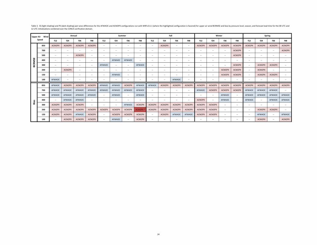
f12 f24 f36 f48 f12 f24 f36 f48 f12 f24 f36 f48 f12 f24 f36 f48 f12 f24 f36 f48

850 ACM2PX ACM2PX ACM2PX ACM2PX -- -- -- -- -- ACM2PX -- -- ACM2PX ACM2PX ACM2PX ACM2PX ACM2PX ACM2PX ACM2PX ACM2PX

700 -- -- -- -- -- -- -- -- -- -- -- -- -- -- -- ACM2PX -- -- -- ACM2PX

500 -- -- ACM2PX -- -- -- -- -- -- -- -- -- -- -- -- ACM2PX -- -- -- --

400 -- -- -- -- -- AFWAOC AFWAOC -- -- -- -- -- -- -- -- -- -- -- -- --

300 -- -- -- -- AFWAOC -- -- AFWAOC -- -- -- -- -- -- -- ACM2PX -- ACM2PX ACM2PX --

200 -- ACM2PX -- -- -- -- -- -- -- -- -- -- -- -- ACM2PX ACM2PX -- ACM2PX -- --

150 -- -- -- -- -- AFWAOC -- -- -- -- -- -- -- -- ACM2PX ACM2PX -- ACM2PX ACM2PX --

100 AFWAOC -- -- -- -- -- -- -- -- -- AFWAOC -- -- -- -- -- -- -- -- --

850 AFWAOC ACM2PX ACM2PX ACM2PX AFWAOC AFWAOC ACM2PX AFWAOC AFWAOC ACM2PX ACM2PX ACM2PX ACM2PX ACM2PX ACM2PX ACM2PX ACM2PX ACM2PX ACM2PX ACM2PX

700 AFWAOC AFWAOC AFWAOC AFWAOC AFWAOC AFWAOC AFWAOC AFWAOC -- -- -- -- AFWAOC ACM2PX ACM2PX ACM2PX AFWAOC AFWAOC AFWAOC --

500 AFWAOC AFWAOC AFWAOC AFWAOC -- AFWAOC -- AFWAOC -- -- -- -- -- -- AFWAOC -- AFWAOC AFWAOC AFWAOC AFWAOC

400 -- AFWAOC AFWAOC -- -- -- -- -- -- -- -- -- ACM2PX -- AFWAOC -- AFWAOC -- AFWAOC AFWAOC

300 ACM2PX ACM2PX ACM2PX -- -- -- AFWAOC ACM2PX ACM2PX ACM2PX ACM2PX ACM2PX ACM2PX ACM2PX -- -- -- -- -- --

200 ACM2PX ACM2PX ACM2PX ACM2PX ACM2PX ACM2PX ACM2PX ACM2PX * ACM2PX ACM2PX ACM2PX ACM2PX ACM2PX ACM2PX -- -- -- ACM2PX ACM2PX --

150 ACM2PX ACM2PX AFWAOC ACM2PX -- ACM2PX ACM2PX ACM2PX -- ACM2PX AFWAOC AFWAOC ACM2PX ACM2PX -- -- -- AFWAOC -- AFWAOC

100 -- ACM2PX ACM2PX ACM2PX -- AFWAOC -- ACM2PX -- -- -- -- -- -- -- -- -- ACM2PX -- ACM2PX

Bias

Upper Air Wind Speed

Annual Summer

Table 3. SS (light shading) and PS (dark shading) pair-wise differences for the AFWAOC and ACM2PX configurations run with WRFv3.6.1 (where the highlighted configuration is favored) for upper air wind BCRMSE and bias by pressure level, season, and forecast lead time for the 00 UTC and 12 UTC initializations combined over the CONUS verification domain.

Fall Winter SpringBC

RMSE

24

f03 f06 f09 f12 f15 f18 f21 f24 f27 f30 f33 f36 f39 f42 f45 f48

Annual ACM2PX * -- -- -- ACM2PX * ACM2PX * ACM2PX ACM2PX * ACM2PX * ACM2PX * ACM2PX * ACM2PX * ACM2PX * ACM2PX * -- ACM2PX *

Summer ACM2PX * -- -- -- ACM2PX * -- -- ACM2PX * ACM2PX * ACM2PX * ACM2PX * ACM2PX * ACM2PX * -- -- ACM2PX *

Fall AFWAOC * AFWAOC * -- -- ACM2PX * ACM2PX * ACM2PX ACM2PX * ACM2PX * ACM2PX * ACM2PX * -- ACM2PX * ACM2PX * -- ACM2PX *

Winter -- -- -- -- -- ACM2PX * ACM2PX * ACM2PX * ACM2PX * -- -- -- ACM2PX * ACM2PX * -- ACM2PX *

Spring ACM2PX * ACM2PX * -- -- ACM2PX * ACM2PX * -- ACM2PX * ACM2PX * ACM2PX * ACM2PX * ACM2PX * -- -- -- ACM2PX *

Annual ACM2PX -- -- ACM2PX * ACM2PX * ACM2PX * ACM2PX * ACM2PX ACM2PX * ACM2PX * ACM2PX * ACM2PX * ACM2PX * ACM2PX * ACM2PX * ACM2PX *

Summer ACM2PX * -- -- ACM2PX * ACM2PX * ACM2PX * ACM2PX * ACM2PX ACM2PX * -- -- ACM2PX * ACM2PX * ACM2PX * ACM2PX * ACM2PX *

Fall -- ACM2PX * -- ACM2PX * ACM2PX ACM2PX ACM2PX * ACM2PX ACM2PX * -- -- ACM2PX * -- -- -- --

Winter -- -- -- ACM2PX * ACM2PX * ACM2PX * -- ACM2PX * ACM2PX * ACM2PX * ACM2PX * ACM2PX * ACM2PX * ACM2PX * -- --

Spring ACM2PX * -- -- ACM2PX * ACM2PX * ACM2PX * ACM2PX * ACM2PX * ACM2PX * ACM2PX * ACM2PX * ACM2PX * ACM2PX * ACM2PX * ACM2PX * ACM2PX *

Annual ACM2PX * ACM2PX * ACM2PX * ACM2PX * AFWAOC * -- -- ACM2PX * ACM2PX * ACM2PX * ACM2PX * ACM2PX * AFWAOC * -- -- ACM2PX *

Summer ACM2PX * ACM2PX * ACM2PX * ACM2PX * ACM2PX * AFWAOC * AFWAOC * AFWAOC * ACM2PX * ACM2PX * ACM2PX * AFWAOC * ACM2PX * ACM2PX * ACM2PX * ACM2PX *

Fall -- -- -- ACM2PX * AFWAOC * AFWAOC * AFWAOC * ACM2PX * -- -- ACM2PX * ACM2PX * AFWAOC * AFWAOC * AFWAOC * ACM2PX *

Winter -- -- -- -- AFWAOC * -- ACM2PX * ACM2PX * -- -- -- -- -- -- ACM2PX * ACM2PX *

Spring ACM2PX * ACM2PX * ACM2PX * ACM2PX * -- ACM2PX * ACM2PX * ACM2PX * ACM2PX * ACM2PX * ACM2PX * ACM2PX * ACM2PX * ACM2PX * ACM2PX * ACM2PX *

Annual AFWAOC * AFWAOC * -- -- ACM2PX * -- ACM2PX * AFWAOC * AFWAOC * AFWAOC * -- -- -- -- ACM2PX * AFWAOC *

Summer AFWAOC * AFWAOC * AFWAOC * AFWAOC * ACM2PX * ACM2PX * ACM2PX * AFWAOC * ACM2PX * ACM2PX * AFWAOC * AFWAOC * -- ACM2PX * AFWAOC * AFWAOC *

Fall AFWAOC * AFWAOC * AFWAOC * -- AFWAOC * -- -- AFWAOC * AFWAOC * AFWAOC * AFWAOC * ACM2PX * AFWAOC * -- ACM2PX * AFWAOC *

Winter AFWAOC * -- ACM2PX * ACM2PX * -- -- -- -- AFWAOC * -- -- ACM2PX * -- -- -- --

Spring AFWAOC * ACM2PX * ACM2PX * ACM2PX * ACM2PX * -- ACM2PX * ACM2PX * -- AFWAOC * ACM2PX * ACM2PX * ACM2PX * ACM2PX * ACM2PX * --

Table 4. SS (light shading) and PS (dark shading) pair-wise differences for the AFWAOC and ACM2PX configurations run with WRFv3.6.1 (where the highlighted configuration is favored) for surface temperature BCRMSE and bias by season and forecast lead time for the 00 UTC and 12 UTC initializations separately over the CONUS verification domain.

Surface TemperatureBi

as

00 U

TC In

itial

izat

ions

12 U

TC In

itial

izat

ions

BCRM

SE 00 U

TC In

itial

izat

ions

12 U

TC In

itial

izat

ions

25

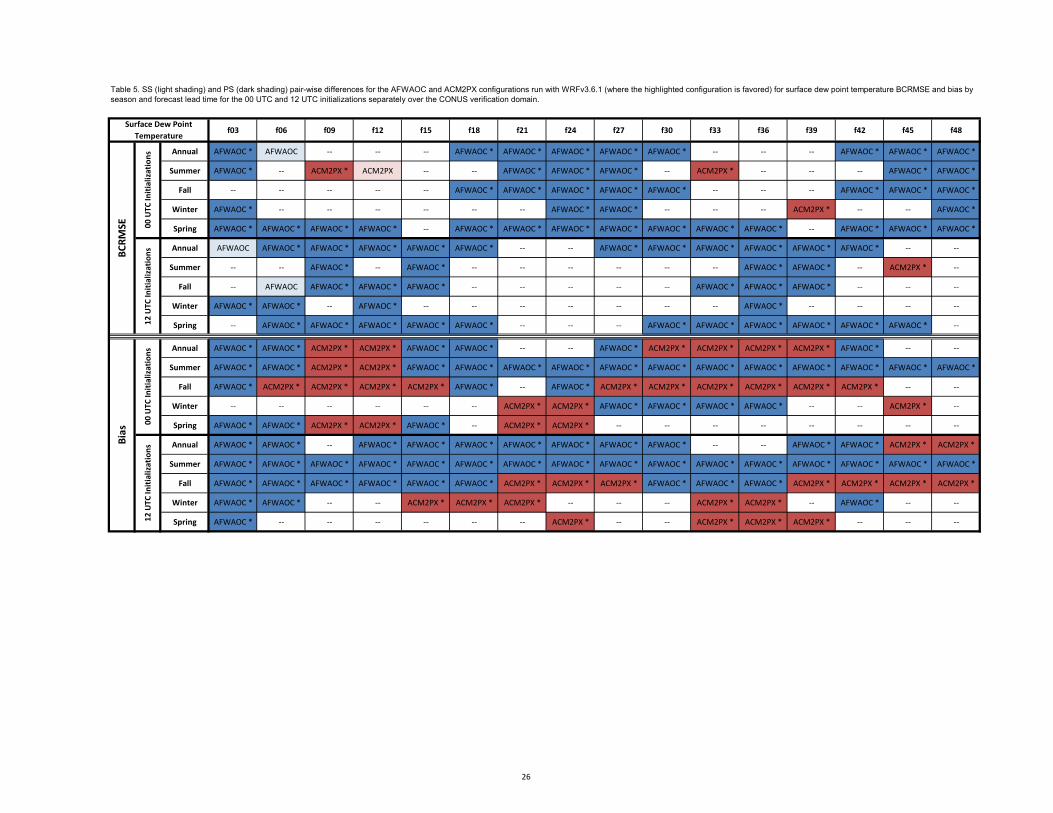
f03 f06 f09 f12 f15 f18 f21 f24 f27 f30 f33 f36 f39 f42 f45 f48

Annual AFWAOC * AFWAOC -- -- -- AFWAOC * AFWAOC * AFWAOC * AFWAOC * AFWAOC * -- -- -- AFWAOC * AFWAOC * AFWAOC *

Summer AFWAOC * -- ACM2PX * ACM2PX -- -- AFWAOC * AFWAOC * AFWAOC * -- ACM2PX * -- -- -- AFWAOC * AFWAOC *

Fall -- -- -- -- -- AFWAOC * AFWAOC * AFWAOC * AFWAOC * AFWAOC * -- -- -- AFWAOC * AFWAOC * AFWAOC *

Winter AFWAOC * -- -- -- -- -- -- AFWAOC * AFWAOC * -- -- -- ACM2PX * -- -- AFWAOC *

Spring AFWAOC * AFWAOC * AFWAOC * AFWAOC * -- AFWAOC * AFWAOC * AFWAOC * AFWAOC * AFWAOC * AFWAOC * AFWAOC * -- AFWAOC * AFWAOC * AFWAOC *

Annual AFWAOC AFWAOC * AFWAOC * AFWAOC * AFWAOC * AFWAOC * -- -- AFWAOC * AFWAOC * AFWAOC * AFWAOC * AFWAOC * AFWAOC * -- --

Summer -- -- AFWAOC * -- AFWAOC * -- -- -- -- -- -- AFWAOC * AFWAOC * -- ACM2PX * --

Fall -- AFWAOC AFWAOC * AFWAOC * AFWAOC * -- -- -- -- -- AFWAOC * AFWAOC * AFWAOC * -- -- --

Winter AFWAOC * AFWAOC * -- AFWAOC * -- -- -- -- -- -- -- AFWAOC * -- -- -- --

Spring -- AFWAOC * AFWAOC * AFWAOC * AFWAOC * AFWAOC * -- -- -- AFWAOC * AFWAOC * AFWAOC * AFWAOC * AFWAOC * AFWAOC * --

Annual AFWAOC * AFWAOC * ACM2PX * ACM2PX * AFWAOC * AFWAOC * -- -- AFWAOC * ACM2PX * ACM2PX * ACM2PX * ACM2PX * AFWAOC * -- --

Summer AFWAOC * AFWAOC * ACM2PX * ACM2PX * AFWAOC * AFWAOC * AFWAOC * AFWAOC * AFWAOC * AFWAOC * AFWAOC * AFWAOC * AFWAOC * AFWAOC * AFWAOC * AFWAOC *

Fall AFWAOC * ACM2PX * ACM2PX * ACM2PX * ACM2PX * AFWAOC * -- AFWAOC * ACM2PX * ACM2PX * ACM2PX * ACM2PX * ACM2PX * ACM2PX * -- --

Winter -- -- -- -- -- -- ACM2PX * ACM2PX * AFWAOC * AFWAOC * AFWAOC * AFWAOC * -- -- ACM2PX * --

Spring AFWAOC * AFWAOC * ACM2PX * ACM2PX * AFWAOC * -- ACM2PX * ACM2PX * -- -- -- -- -- -- -- --

Annual AFWAOC * AFWAOC * -- AFWAOC * AFWAOC * AFWAOC * AFWAOC * AFWAOC * AFWAOC * AFWAOC * -- -- AFWAOC * AFWAOC * ACM2PX * ACM2PX *

Summer AFWAOC * AFWAOC * AFWAOC * AFWAOC * AFWAOC * AFWAOC * AFWAOC * AFWAOC * AFWAOC * AFWAOC * AFWAOC * AFWAOC * AFWAOC * AFWAOC * AFWAOC * AFWAOC *

Fall AFWAOC * AFWAOC * AFWAOC * AFWAOC * AFWAOC * AFWAOC * ACM2PX * ACM2PX * ACM2PX * AFWAOC * AFWAOC * AFWAOC * ACM2PX * ACM2PX * ACM2PX * ACM2PX *

Winter AFWAOC * AFWAOC * -- -- ACM2PX * ACM2PX * ACM2PX * -- -- -- ACM2PX * ACM2PX * -- AFWAOC * -- --

Spring AFWAOC * -- -- -- -- -- -- ACM2PX * -- -- ACM2PX * ACM2PX * ACM2PX * -- -- --

Bias

00 U

TC In

itial

izat

ions

12 U

TC In

itial

izat

ions

Table 5. SS (light shading) and PS (dark shading) pair-wise differences for the AFWAOC and ACM2PX configurations run with WRFv3.6.1 (where the highlighted configuration is favored) for surface dew point temperature BCRMSE and bias by season and forecast lead time for the 00 UTC and 12 UTC initializations separately over the CONUS verification domain.

Surface Dew Point Temperature

BCRM

SE 00 U

TC In

itial

izat

ions

12 U

TC In

itial

izat

ions

26

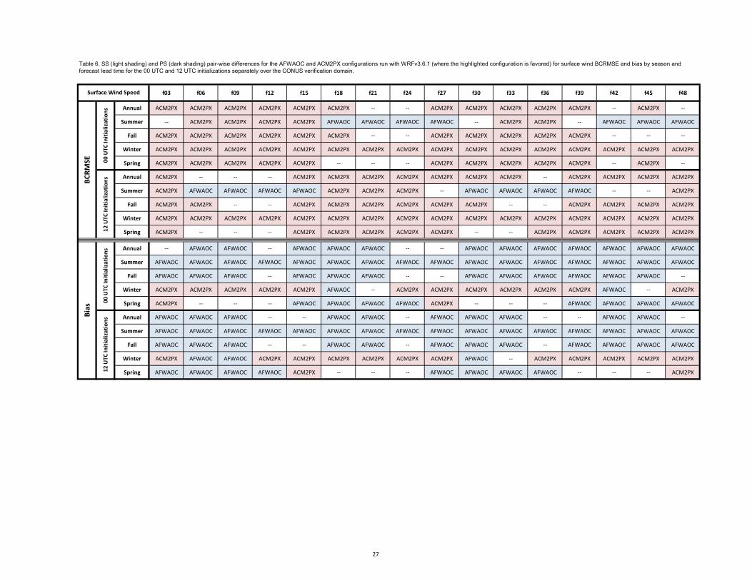
f03 f06 f09 f12 f15 f18 f21 f24 f27 f30 f33 f36 f39 f42 f45 f48

Annual ACM2PX ACM2PX ACM2PX ACM2PX ACM2PX ACM2PX -- -- ACM2PX ACM2PX ACM2PX ACM2PX ACM2PX -- ACM2PX --

Summer -- ACM2PX ACM2PX ACM2PX ACM2PX AFWAOC AFWAOC AFWAOC AFWAOC -- ACM2PX ACM2PX -- AFWAOC AFWAOC AFWAOC

Fall ACM2PX ACM2PX ACM2PX ACM2PX ACM2PX ACM2PX -- -- ACM2PX ACM2PX ACM2PX ACM2PX ACM2PX -- -- --

Winter ACM2PX ACM2PX ACM2PX ACM2PX ACM2PX ACM2PX ACM2PX ACM2PX ACM2PX ACM2PX ACM2PX ACM2PX ACM2PX ACM2PX ACM2PX ACM2PX

Spring ACM2PX ACM2PX ACM2PX ACM2PX ACM2PX -- -- -- ACM2PX ACM2PX ACM2PX ACM2PX ACM2PX -- ACM2PX --

Annual ACM2PX -- -- -- ACM2PX ACM2PX ACM2PX ACM2PX ACM2PX ACM2PX ACM2PX -- ACM2PX ACM2PX ACM2PX ACM2PX

Summer ACM2PX AFWAOC AFWAOC AFWAOC AFWAOC ACM2PX ACM2PX ACM2PX -- AFWAOC AFWAOC AFWAOC AFWAOC -- -- ACM2PX

Fall ACM2PX ACM2PX -- -- ACM2PX ACM2PX ACM2PX ACM2PX ACM2PX ACM2PX -- -- ACM2PX ACM2PX ACM2PX ACM2PX

Winter ACM2PX ACM2PX ACM2PX ACM2PX ACM2PX ACM2PX ACM2PX ACM2PX ACM2PX ACM2PX ACM2PX ACM2PX ACM2PX ACM2PX ACM2PX ACM2PX

Spring ACM2PX -- -- -- ACM2PX ACM2PX ACM2PX ACM2PX ACM2PX -- -- ACM2PX ACM2PX ACM2PX ACM2PX ACM2PX

Annual -- AFWAOC AFWAOC -- AFWAOC AFWAOC AFWAOC -- -- AFWAOC AFWAOC AFWAOC AFWAOC AFWAOC AFWAOC AFWAOC

Summer AFWAOC AFWAOC AFWAOC AFWAOC AFWAOC AFWAOC AFWAOC AFWAOC AFWAOC AFWAOC AFWAOC AFWAOC AFWAOC AFWAOC AFWAOC AFWAOC

Fall AFWAOC AFWAOC AFWAOC -- AFWAOC AFWAOC AFWAOC -- -- AFWAOC AFWAOC AFWAOC AFWAOC AFWAOC AFWAOC --

Winter ACM2PX ACM2PX ACM2PX ACM2PX ACM2PX AFWAOC -- ACM2PX ACM2PX ACM2PX ACM2PX ACM2PX ACM2PX AFWAOC -- ACM2PX

Spring ACM2PX -- -- -- AFWAOC AFWAOC AFWAOC AFWAOC ACM2PX -- -- -- AFWAOC AFWAOC AFWAOC AFWAOC

Annual AFWAOC AFWAOC AFWAOC -- -- AFWAOC AFWAOC -- AFWAOC AFWAOC AFWAOC -- -- AFWAOC AFWAOC --

Summer AFWAOC AFWAOC AFWAOC AFWAOC AFWAOC AFWAOC AFWAOC AFWAOC AFWAOC AFWAOC AFWAOC AFWAOC AFWAOC AFWAOC AFWAOC AFWAOC

Fall AFWAOC AFWAOC AFWAOC -- -- AFWAOC AFWAOC -- AFWAOC AFWAOC AFWAOC -- AFWAOC AFWAOC AFWAOC AFWAOC

Winter ACM2PX AFWAOC AFWAOC ACM2PX ACM2PX ACM2PX ACM2PX ACM2PX ACM2PX AFWAOC -- ACM2PX ACM2PX ACM2PX ACM2PX ACM2PX

Spring AFWAOC AFWAOC AFWAOC AFWAOC ACM2PX -- -- -- AFWAOC AFWAOC AFWAOC AFWAOC -- -- -- ACM2PX

Bias

00 U

TC In

itial

izat

ions

12 U

TC In

itial

izat

ions

Table 6. SS (light shading) and PS (dark shading) pair-wise differences for the AFWAOC and ACM2PX configurations run with WRFv3.6.1 (where the highlighted configuration is favored) for surface wind BCRMSE and bias by season and forecast lead time for the 00 UTC and 12 UTC initializations separately over the CONUS verification domain.

Surface Wind SpeedBC

RMSE 00

UTC

Initi

aliz

atio

ns12

UTC

Initi

aliz

atio

ns

27

>0.01 >0.02 >0.05 >0.1 >0.15 >0.25 >0.35 >0.5 >1 >0.01 >0.02 >0.05 >0.1 >0.15 >0.25 >0.35 >0.5 >1

f12 -- -- -- -- -- -- -- -- -- -- -- -- -- -- -- -- -- --

f24 -- -- -- -- -- -- -- -- -- -- -- -- -- -- -- -- -- ACM2PX

f36 -- -- -- -- -- -- -- -- -- -- -- -- -- -- -- -- -- --

f48 -- -- -- -- -- -- -- -- -- -- -- -- -- -- -- -- -- --

f12 -- -- -- -- -- -- -- -- -- -- -- -- -- -- -- -- -- --

f24 -- -- -- -- -- -- -- -- -- -- -- -- -- -- -- -- -- --

f36 -- -- -- -- -- -- -- -- -- -- -- -- -- -- -- -- -- --

f48 -- -- -- AFWAOC AFWAOC -- -- -- -- -- -- -- -- -- -- -- -- --

f12 -- -- -- -- -- -- -- -- -- -- -- -- -- -- -- -- -- --

f24 -- -- -- -- -- -- -- -- -- -- -- -- -- -- -- -- -- --

f36 -- -- -- -- -- -- -- -- -- -- -- -- -- -- -- -- -- --

f48 -- -- -- -- -- -- -- -- -- -- -- -- -- -- -- -- -- --

f12 -- -- -- -- -- -- -- -- -- -- -- -- -- -- -- -- -- --

f24 -- -- -- -- -- -- -- -- -- -- -- -- -- -- -- -- -- --

f36 -- -- -- -- -- -- -- -- -- -- -- -- -- -- -- -- -- --

f48 -- -- -- -- -- -- -- -- -- -- -- -- -- -- -- -- -- --

f12 -- -- -- -- -- -- -- -- -- -- -- -- -- -- -- -- -- --

f24 -- -- -- -- -- -- -- -- -- -- -- -- -- -- -- -- -- --

f36 -- -- -- -- -- -- -- -- -- -- -- -- -- -- -- -- -- --

f48 -- -- -- -- -- -- -- -- -- -- -- -- -- -- -- -- -- --

f12 -- -- -- -- -- -- -- -- -- -- -- -- -- -- -- -- -- --

f24 -- -- -- -- -- -- -- -- -- -- -- -- -- -- -- -- -- --

f36 -- -- -- -- -- -- -- -- -- -- -- -- -- -- -- -- -- --

f48 -- -- -- -- ACM2PX -- -- -- -- -- -- -- -- -- -- -- -- --

f12 -- -- -- -- -- -- -- -- -- -- -- -- -- -- -- -- -- --

f24 -- -- -- -- -- -- -- -- -- -- -- -- -- -- -- -- -- --

f36 -- -- -- -- -- -- -- -- -- -- -- -- -- -- ACM2PX -- -- --

f48 -- -- -- -- -- -- -- -- -- -- -- -- -- -- -- -- -- --

f12 -- -- -- -- -- -- -- -- -- -- -- -- -- -- -- -- -- --

f24 -- -- -- -- -- -- -- -- -- -- -- -- -- -- -- -- -- --

f36 -- -- -- -- -- -- -- -- -- -- -- -- -- -- -- -- -- --

f48 -- -- -- -- -- -- -- -- -- -- -- -- -- -- -- -- -- --

f12 -- -- -- -- -- -- -- -- -- -- -- -- -- -- -- -- -- --

f24 -- -- -- -- -- -- -- -- -- -- -- -- -- -- -- -- -- --

f36 -- -- -- -- -- -- -- -- -- -- -- -- -- -- -- -- -- --

f48 -- -- -- -- -- -- -- -- -- -- -- -- -- -- -- -- -- --

f12 -- -- -- -- -- -- -- -- -- -- -- -- -- -- -- -- -- --

f24 -- -- -- -- -- -- -- -- -- -- -- -- -- -- -- -- -- --

f36 -- -- -- -- -- -- -- -- -- -- -- -- -- -- -- -- -- --

f48 -- -- -- -- -- -- -- -- -- -- -- -- -- -- -- -- -- --

Table 7. SS differences for the AFWAOC and ACM2PX configurations run with WRFv3.6.1 (where the highlighted configuration is favored) for 3-hour QPF GSS and frequency bias by season, forecast lead time, and threshold for the 00 UTC and 12 UTC initializations separately over the CONUS verification domain.

00 UTC Initializations 12 UTC InitializationsGi

lber

t Ski

ll Sc

ore

3-hour QPF

Annu

alSu

mm

erFa

llSp

ring

Win

ter

Sprin

g

Freq

uenc

y Bi

as

Annu

alSu

mm

erFa

llW

inte

r

28

Annual f36 -- -- -- -- -- -- -- -- --

Summer f36 -- -- -- -- -- -- -- -- --

Fall f36 -- -- -- -- -- -- -- -- --

Winter f36 -- -- -- -- -- -- -- -- --

Spring f36 -- -- -- -- -- -- -- -- --

f24 -- -- -- -- -- -- -- -- --

f48 -- -- -- -- -- -- -- -- --

f24 -- -- -- -- -- -- -- -- --

f48 -- -- -- -- -- -- -- -- --

f24 -- -- -- -- -- -- -- -- --

f48 -- -- -- -- -- -- -- -- --

f24 -- -- -- -- -- -- -- -- --

f48 -- -- -- -- -- -- -- -- --

f24 -- -- -- -- -- -- -- -- --

f48 -- -- -- -- -- -- -- -- --

Annual f36 -- -- -- -- -- -- -- -- --

Summer f36 -- -- -- -- -- -- -- -- --

Fall f36 -- -- -- -- -- -- -- -- --

Winter f36 -- -- -- -- -- -- -- -- --

Spring f36 -- -- -- -- -- -- -- -- --

f24 -- -- -- -- -- -- -- -- --

f48 -- -- -- -- -- -- -- -- --

f24 -- -- -- -- -- -- -- -- --

f48 -- -- -- -- -- -- -- -- --

f24 -- -- -- -- -- -- -- -- --

f48 -- -- -- -- -- -- -- -- --

f24 -- -- -- -- -- -- -- -- --

f48 -- -- -- -- -- -- -- -- --

f24 -- -- -- -- -- -- -- -- --

f48 -- -- -- -- -- -- -- -- --

Table 8. SS differences for the AFWAOC and ACM2PX configurations run with WRFv3.6.1 (where the highlighted configuration is favored) for 24-hour QPF GSS and frequency bias by season, forecast lead time, and threshold for the 00 UTC and 12 UTC initializations separately over the CONUS verification domain.

>1.5 >2 >300

UTC

Initi

aliz

atio

ns>0.01 >0.25 >0.5 >0.75 >1 >1.25Daily QPF

Gilb

ert S

kill

Scor

eFr

eque

ncy

Bias

00 U

TC In

itial

izat

ions

12 U

TC In

itial

izat

ions

Annual

Summer

Fall

Winter

Spring

12 U

TC In

itial

izat

ions

Annual

Summer

Fall

Winter

Spring

29

30

Figure 1. Overview of 6-hr “warm start” spin-up.

Figure 2. WRF-ARW computational domain.

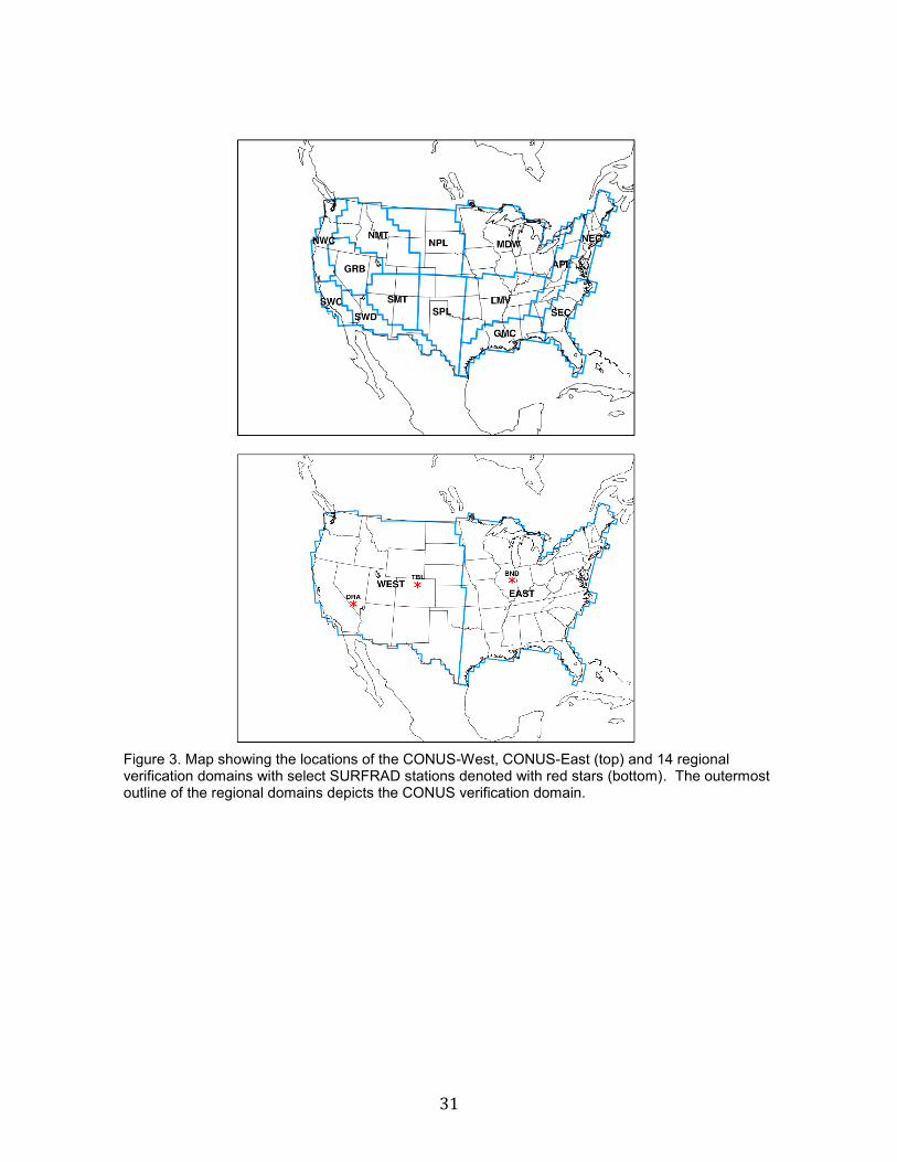
31

Figure 3. Map showing the locations of the CONUS-West, CONUS-East (top) and 14 regional verification domains with select SURFRAD stations denoted with red stars (bottom). The outermost outline of the regional domains depicts the CONUS verification domain.

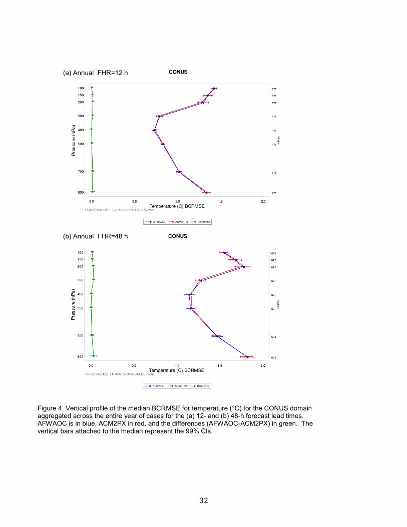
32

Figure 4. Vertical profile of the median BCRMSE for temperature (°C) for the CONUS domain aggregated across the entire year of cases for the (a) 12- and (b) 48-h forecast lead times. AFWAOC is in blue, ACM2PX in red, and the differences (AFWAOC-ACM2PX) in green. The vertical bars attached to the median represent the 99% CIs.

(a) Annual FHR=12 h

(b) Annual FHR=48 h

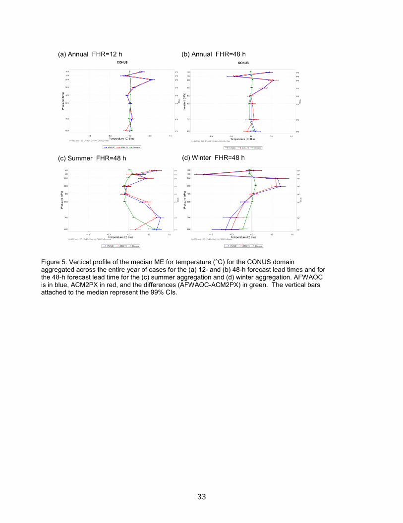
33

Figure 5. Vertical profile of the median ME for temperature (°C) for the CONUS domain aggregated across the entire year of cases for the (a) 12- and (b) 48-h forecast lead times and for the 48-h forecast lead time for the (c) summer aggregation and (d) winter aggregation. AFWAOC is in blue, ACM2PX in red, and the differences (AFWAOC-ACM2PX) in green. The vertical bars attached to the median represent the 99% CIs.

(a) Annual FHR=12 h (b) Annual FHR=48 h

(d) Winter FHR=48 h (c) Summer FHR=48 h

34

Figure 6. Vertical profile of the median BCRMSE for dew point temperature (°C) for the CONUS domain aggregated across the entire year of cases for the (a) 12- and (b) 48-h forecast lead times. AFWAOC is in blue, ACM2PX in red, and the differences (AFWAOC-ACM2PX) in green. The vertical bars attached to the median represent the 99% CIs.

(a) Annual FHR=12 h

(b) Annual FHR=48 h

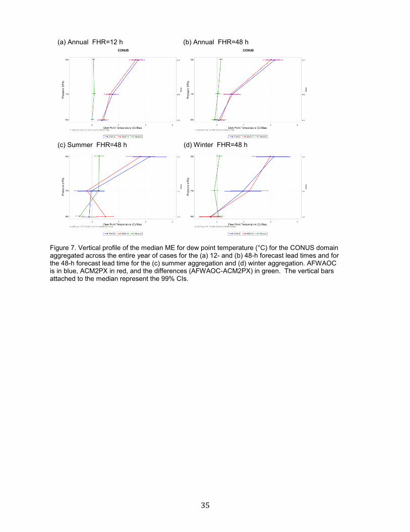
35

Figure 7. Vertical profile of the median ME for dew point temperature (°C) for the CONUS domain aggregated across the entire year of cases for the (a) 12- and (b) 48-h forecast lead times and for the 48-h forecast lead time for the (c) summer aggregation and (d) winter aggregation. AFWAOC is in blue, ACM2PX in red, and the differences (AFWAOC-ACM2PX) in green. The vertical bars attached to the median represent the 99% CIs.

(a) Annual FHR=12 h (b) Annual FHR=48 h

(d) Winter FHR=48 h (c) Summer FHR=48 h

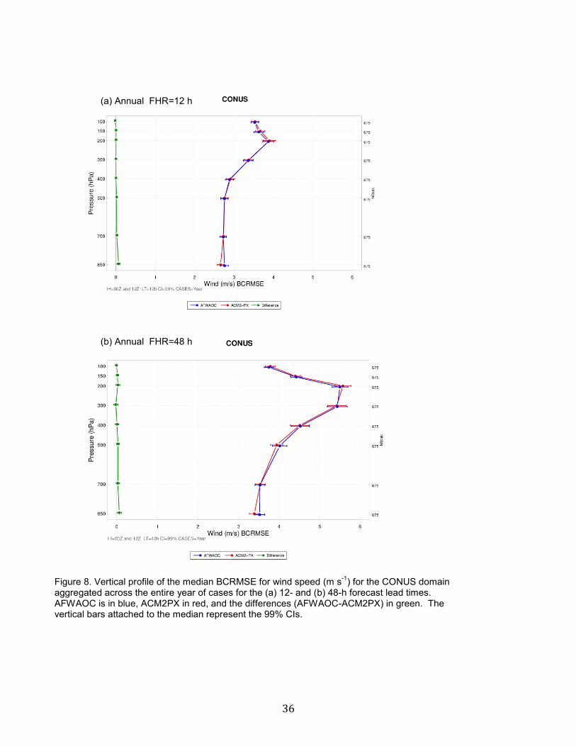
36

Figure 8. Vertical profile of the median BCRMSE for wind speed (m s-1) for the CONUS domain aggregated across the entire year of cases for the (a) 12- and (b) 48-h forecast lead times. AFWAOC is in blue, ACM2PX in red, and the differences (AFWAOC-ACM2PX) in green. The vertical bars attached to the median represent the 99% CIs.

(a) Annual FHR=12 h

(b) Annual FHR=48 h

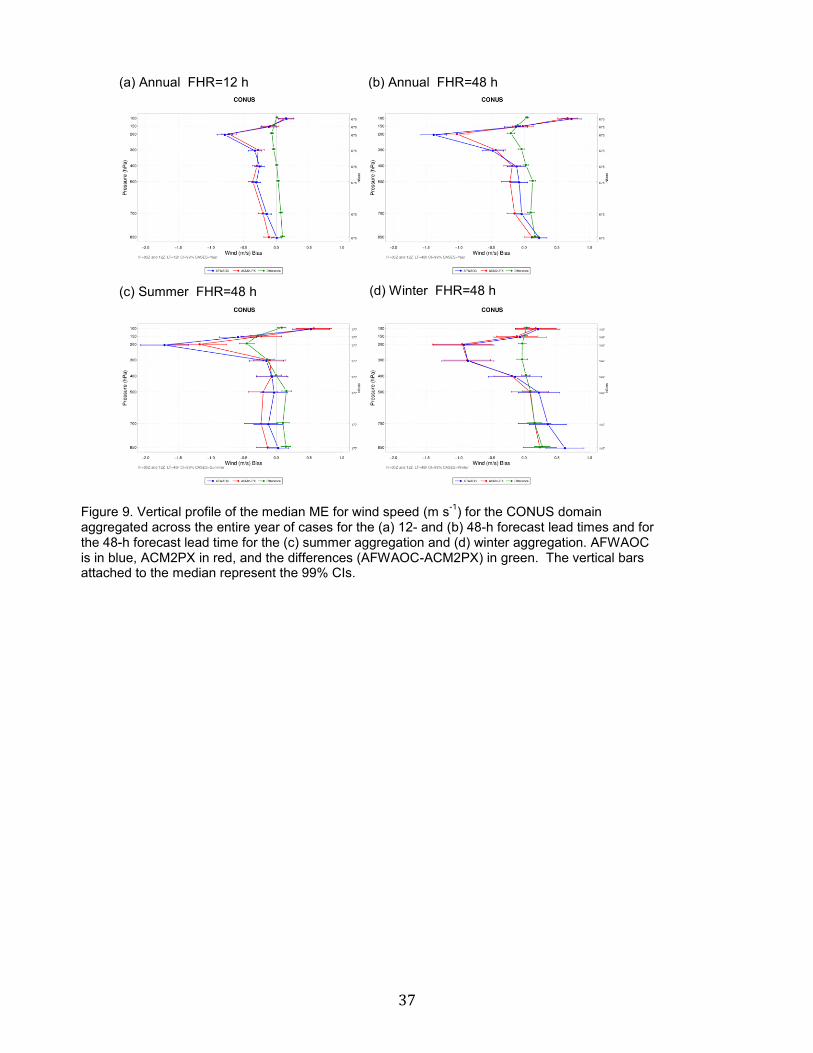
37

Figure 9. Vertical profile of the median ME for wind speed (m s-1) for the CONUS domain aggregated across the entire year of cases for the (a) 12- and (b) 48-h forecast lead times and for the 48-h forecast lead time for the (c) summer aggregation and (d) winter aggregation. AFWAOC is in blue, ACM2PX in red, and the differences (AFWAOC-ACM2PX) in green. The vertical bars attached to the median represent the 99% CIs.

(a) Annual FHR=12 h (b) Annual FHR=48 h

(d) Winter FHR=48 h (c) Summer FHR=48 h

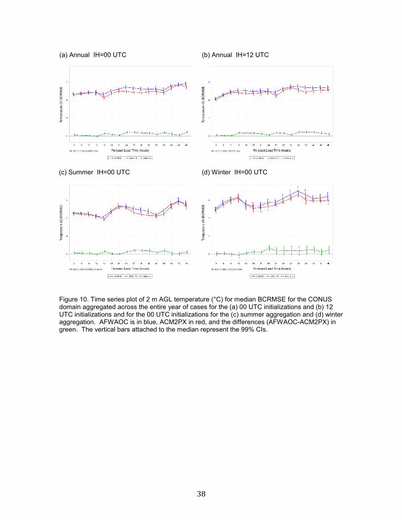
38

Figure 10. Time series plot of 2 m AGL temperature (°C) for median BCRMSE for the CONUS domain aggregated across the entire year of cases for the (a) 00 UTC initializations and (b) 12 UTC initializations and for the 00 UTC initializations for the (c) summer aggregation and (d) winter aggregation. AFWAOC is in blue, ACM2PX in red, and the differences (AFWAOC-ACM2PX) in green. The vertical bars attached to the median represent the 99% CIs.

(a) (b)

(b) IH=12 UTC

(a) Annual IH=00 UTC (b) Annual IH=12 UTC

(d) Winter IH=00 UTC (c) Summer IH=00 UTC

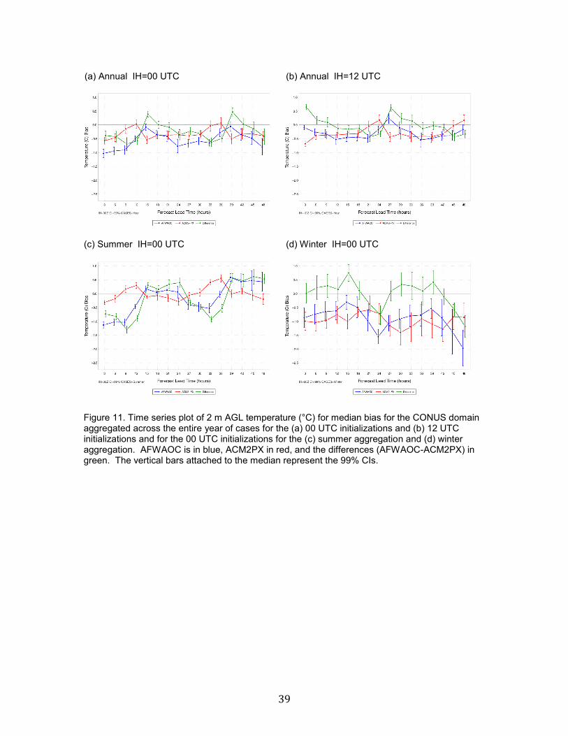
39

Figure 11. Time series plot of 2 m AGL temperature (°C) for median bias for the CONUS domain aggregated across the entire year of cases for the (a) 00 UTC initializations and (b) 12 UTC initializations and for the 00 UTC initializations for the (c) summer aggregation and (d) winter aggregation. AFWAOC is in blue, ACM2PX in red, and the differences (AFWAOC-ACM2PX) in green. The vertical bars attached to the median represent the 99% CIs.

(a) (b)

(a) Annual IH=00 UTC (b) Annual IH=12 UTC

(d) Winter IH=00 UTC (c) Summer IH=00 UTC

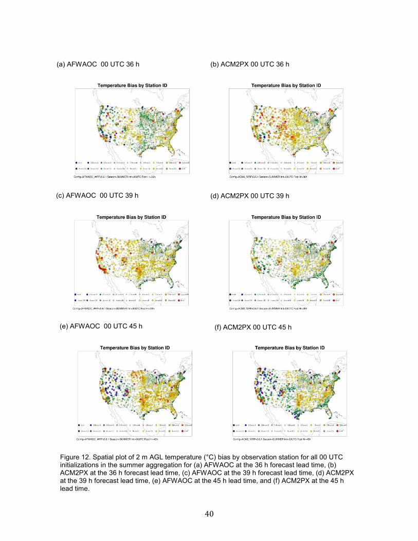
40

(a) AFWAOC 00 UTC 36 h (b) ACM2PX 00 UTC 36 h

(d) ACM2PX 00 UTC 39 h (c) AFWAOC 00 UTC 39 h

Figure 12. Spatial plot of 2 m AGL temperature (°C) bias by observation station for all 00 UTC initializations in the summer aggregation for (a) AFWAOC at the 36 h forecast lead time, (b) ACM2PX at the 36 h forecast lead time, (c) AFWAOC at the 39 h forecast lead time, (d) ACM2PX at the 39 h forecast lead time, (e) AFWAOC at the 45 h lead time, and (f) ACM2PX at the 45 h lead time.

(f) ACM2PX 00 UTC 45 h (e) AFWAOC 00 UTC 45 h

41

(a) AFWAOC 00 UTC 45 h (b) ACM2PX 00 UTC 45 h

Figure 13. Spatial plot of 2 m AGL temperature (°C) bias by observation station for all 00 UTC initializations in the fall aggregation for (a) AFWAOC and (b) ACM2PX at the 45 h forecast lead time.

42

(a) AFWAOC 00 UTC 36 h (b) ACM2PX 00 UTC 36 h

(d) ACM2PX 00 UTC 45 h (c) AFWAOC 00 UTC 45 h

Figure 14. Spatial plot of 2 m AGL temperature (°C) bias by observation station for all 00 UTC initializations in the winter aggregation for (a) AFWAOC at the 36 h forecast lead time, (b) ACM2PX at the 36 h forecast lead time, (c) AFWAOC at the 45 h forecast lead time, and (d) ACM2PX at the 45 h forecast lead time.

43

(a) AFWAOC 00 UTC 45 h (b) ACM2PX 00 UTC 45 h

Figure 15. Spatial plot of 2 m AGL temperature (°C) bias by observation station for all 00 UTC initializations in the spring aggregation for (a) AFWAOC and (b) ACM2PX at the 45 h forecast lead time.

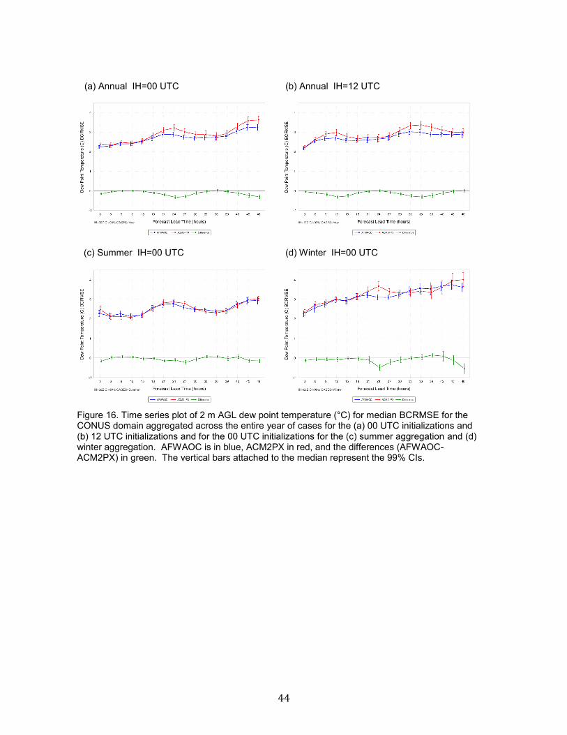
44

Figure 16. Time series plot of 2 m AGL dew point temperature (°C) for median BCRMSE for the CONUS domain aggregated across the entire year of cases for the (a) 00 UTC initializations and (b) 12 UTC initializations and for the 00 UTC initializations for the (c) summer aggregation and (d) winter aggregation. AFWAOC is in blue, ACM2PX in red, and the differences (AFWAOC-ACM2PX) in green. The vertical bars attached to the median represent the 99% CIs.

(a) Annual IH=00 UTC

(d) Winter IH=00 UTC (c) Summer IH=00 UTC

(b) Annual IH=12 UTC

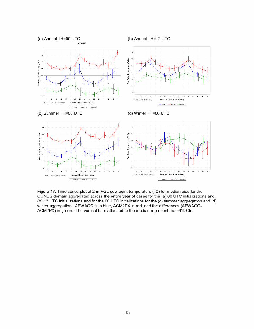
45

Figure 17. Time series plot of 2 m AGL dew point temperature (°C) for median bias for the CONUS domain aggregated across the entire year of cases for the (a) 00 UTC initializations and (b) 12 UTC initializations and for the 00 UTC initializations for the (c) summer aggregation and (d) winter aggregation. AFWAOC is in blue, ACM2PX in red, and the differences (AFWAOC-ACM2PX) in green. The vertical bars attached to the median represent the 99% CIs.

(a) Annual IH=00 UTC (b) Annual IH=12 UTC

(d) Winter IH=00 UTC (c) Summer IH=00 UTC

46

(a) AFWAOC 00 UTC 36 h (b) ACM2PX 00 UTC 36 h

(d) ACM2PX 00 UTC 45 h (c) AFWAOC 00 UTC 45 h

Figure 18. Spatial plot of 2 m AGL dew point temperature (°C) bias by observation station for all 00 UTC initializations in the summer aggregation for (a) AFWAOC at the 36 h forecast lead time, (b) ACM2PX at the 36 h forecast lead time, (c) AFWAOC at the 45 h forecast lead time, and (d) ACM2PX at the 45 h forecast lead time.

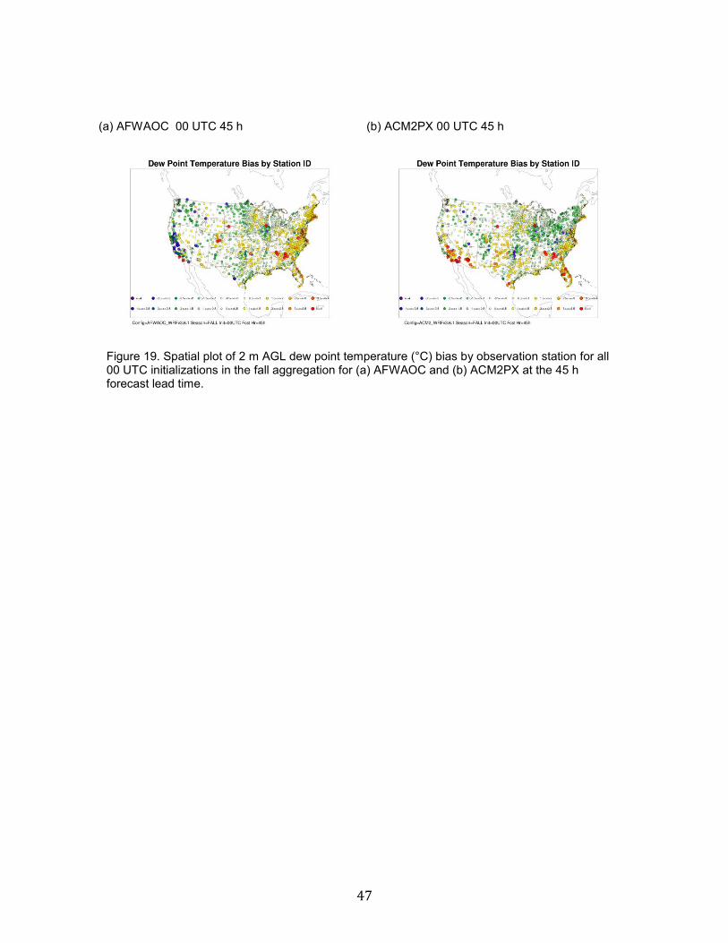
47

(a) AFWAOC 00 UTC 45 h (b) ACM2PX 00 UTC 45 h

Figure 19. Spatial plot of 2 m AGL dew point temperature (°C) bias by observation station for all 00 UTC initializations in the fall aggregation for (a) AFWAOC and (b) ACM2PX at the 45 h forecast lead time.

48

(a) AFWAOC 00 UTC 36 h (b) ACM2PX 00 UTC 36 h

(d) ACM2PX 00 UTC 45 h (c) AFWAOC 00 UTC 45 h

Figure 20. Spatial plot of 2 m AGL dew point temperature (°C) bias by observation station for all 00 UTC initializations in the winter aggregation for (a) AFWAOC at the 36 h forecast lead time, (b) ACM2PX at the 36 h forecast lead time, (c) AFWAOC at the 45 h forecast lead time, and (d) ACM2PX at the 45 h forecast lead time.

49

(a) AFWAOC 00 UTC 45 h (b) ACM2PX 00 UTC 45 h

Figure 21. Spatial plot of 2 m AGL dew point temperature (°C) bias by observation station for all 00 UTC initializations in the spring aggregation for (a) AFWAOC and (b) ACM2PX at the 45 h forecast lead time.

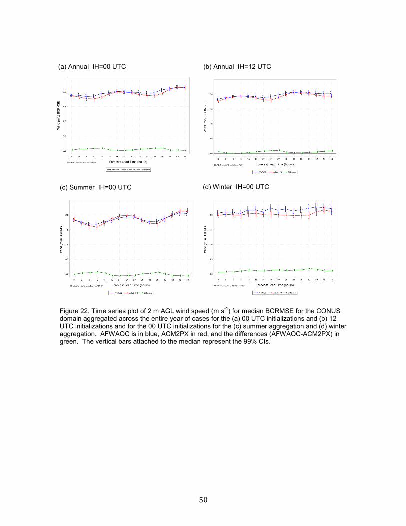
50

Figure 22. Time series plot of 2 m AGL wind speed (m s-1) for median BCRMSE for the CONUS domain aggregated across the entire year of cases for the (a) 00 UTC initializations and (b) 12 UTC initializations and for the 00 UTC initializations for the (c) summer aggregation and (d) winter aggregation. AFWAOC is in blue, ACM2PX in red, and the differences (AFWAOC-ACM2PX) in green. The vertical bars attached to the median represent the 99% CIs.

(a) Annual IH=00 UTC (b) Annual IH=12 UTC

(a) Annual IH=00 UTC (b) Annual IH=12 UTC

(d) Winter IH=00 UTC (c) Summer IH=00 UTC

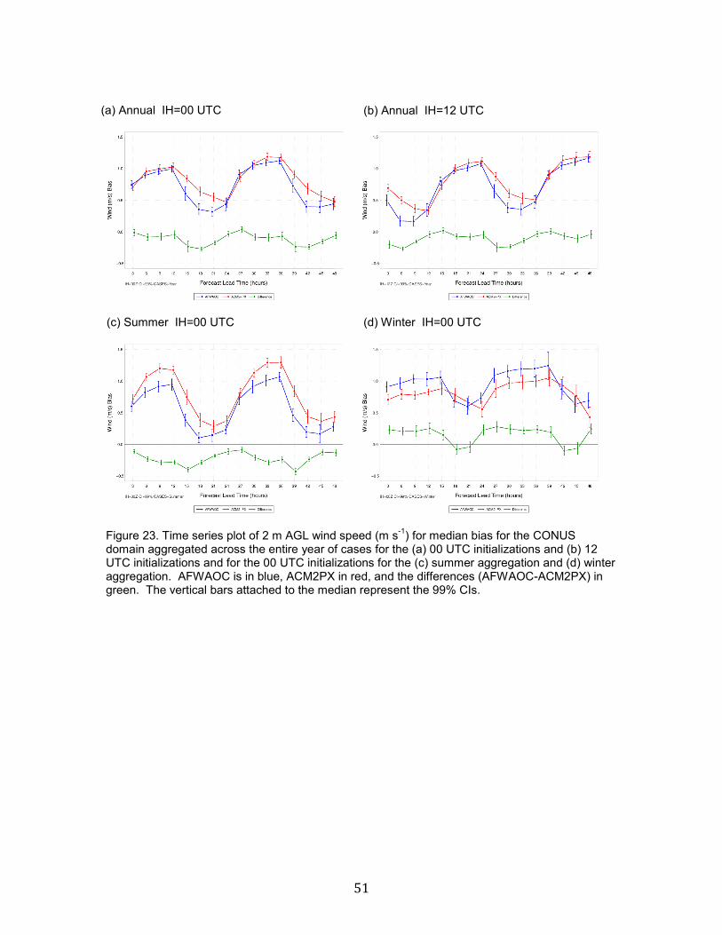
51

Figure 23. Time series plot of 2 m AGL wind speed (m s-1) for median bias for the CONUS domain aggregated across the entire year of cases for the (a) 00 UTC initializations and (b) 12 UTC initializations and for the 00 UTC initializations for the (c) summer aggregation and (d) winter aggregation. AFWAOC is in blue, ACM2PX in red, and the differences (AFWAOC-ACM2PX) in green. The vertical bars attached to the median represent the 99% CIs.

(a) Annual IH=00 UTC (b) Annual IH=12 UTC

(d) Winter IH=00 UTC (c) Summer IH=00 UTC

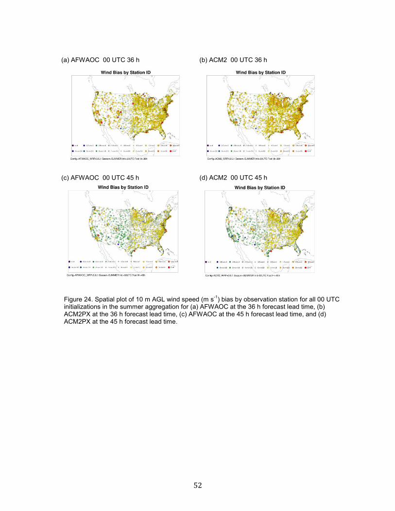
52

Figure 24. Spatial plot of 10 m AGL wind speed (m s-1) bias by observation station for all 00 UTC initializations in the summer aggregation for (a) AFWAOC at the 36 h forecast lead time, (b) ACM2PX at the 36 h forecast lead time, (c) AFWAOC at the 45 h forecast lead time, and (d) ACM2PX at the 45 h forecast lead time.

(c) AFWAOC 00 UTC 45 h (d) ACM2 00 UTC 45 h

(a) AFWAOC 00 UTC 36 h (b) ACM2 00 UTC 36 h

53

(a) AFWAOC 00 UTC 36 h (b) ACM2 00 UTC 36 h

(c) AFWAOC 00 UTC 45 h (d) ACM2 00 UTC 45 h

Figure 25. Spatial plot of 10 m AGL wind speed (m s-1) bias by observation station for all 00 UTC initializations in the winter aggregation for (a) AFWAOC at the 36 h forecast lead time, (b) ACM2PX at the 36 h forecast lead time, (c) AFWAOC at the 45 h forecast lead time, and (d) ACM2PX at the 45 h forecast lead time.

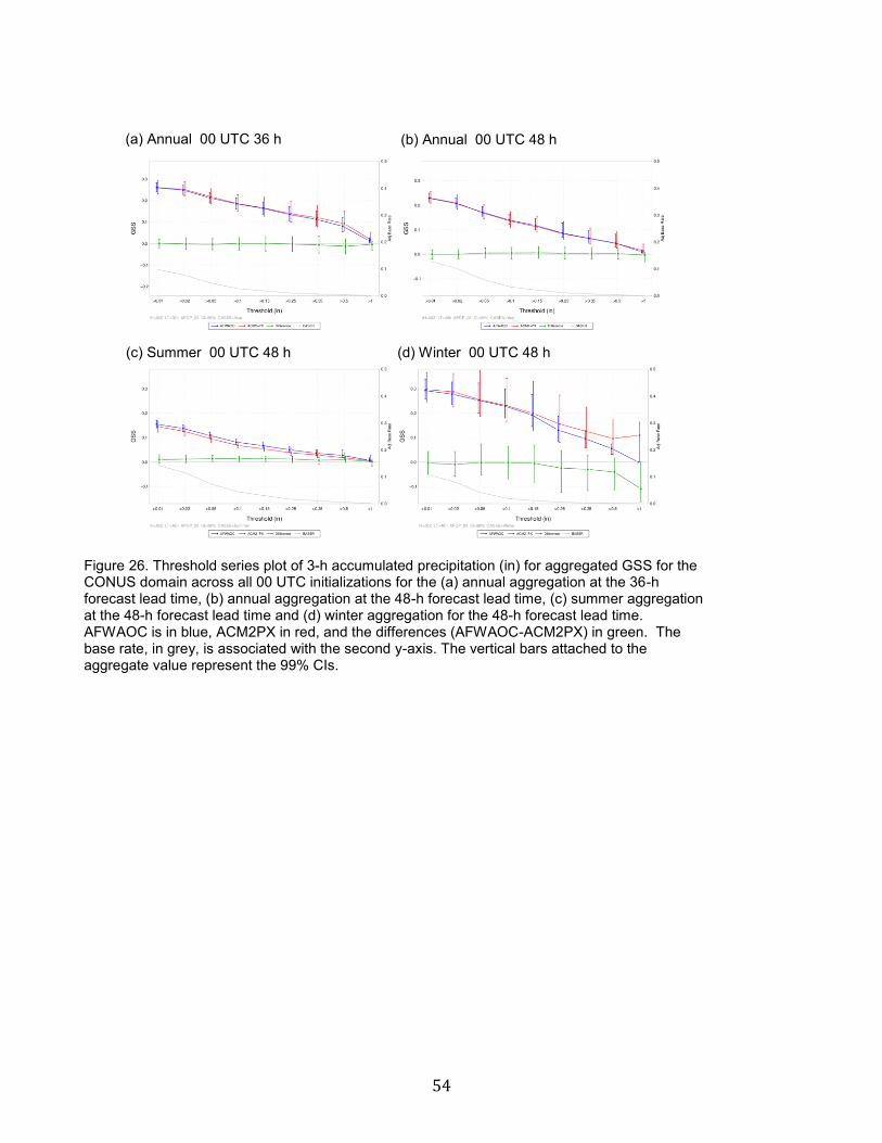
54

Figure 26. Threshold series plot of 3-h accumulated precipitation (in) for aggregated GSS for the CONUS domain across all 00 UTC initializations for the (a) annual aggregation at the 36-h forecast lead time, (b) annual aggregation at the 48-h forecast lead time, (c) summer aggregation at the 48-h forecast lead time and (d) winter aggregation for the 48-h forecast lead time. AFWAOC is in blue, ACM2PX in red, and the differences (AFWAOC-ACM2PX) in green. The base rate, in grey, is associated with the second y-axis. The vertical bars attached to the aggregate value represent the 99% CIs.

(a) Annual 00 UTC 36 h (b) Annual 00 UTC 48 h

(d) Winter 00 UTC 48 h (c) Summer 00 UTC 48 h

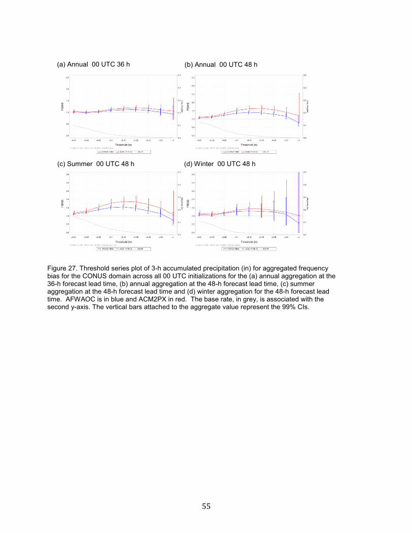
55

Figure 27. Threshold series plot of 3-h accumulated precipitation (in) for aggregated frequency bias for the CONUS domain across all 00 UTC initializations for the (a) annual aggregation at the 36-h forecast lead time, (b) annual aggregation at the 48-h forecast lead time, (c) summer aggregation at the 48-h forecast lead time and (d) winter aggregation for the 48-h forecast lead time. AFWAOC is in blue and ACM2PX in red. The base rate, in grey, is associated with the second y-axis. The vertical bars attached to the aggregate value represent the 99% CIs.

(a) Annual 00 UTC 36 h (b) Annual 00 UTC 48 h

(d) Winter 00 UTC 48 h (c) Summer 00 UTC 48 h

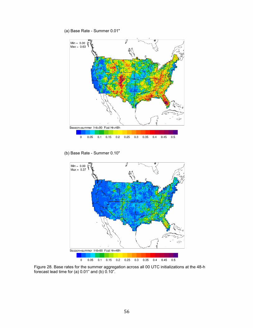
56

Figure 28. Base rates for the summer aggregation across all 00 UTC initializations at the 48-h forecast lead time for (a) 0.01” and (b) 0.10”.

(a) Base Rate - Summer 0.01"

(b) Base Rate - Summer 0.10"

57

Figure 29. Gilbert skill score at the 0.01” threshold for the summer aggregation across all 00 UTC initializations at the 48-h forecast lead time for (a) AFWAOC, (b) ACM2PX, and (C) AFWAOC – ACM2-PX.

(a) AFWAOC – 0.01" (b) ACM2PX – 0.01"

(c) AFWAOC – ACM2PX – 0.01"

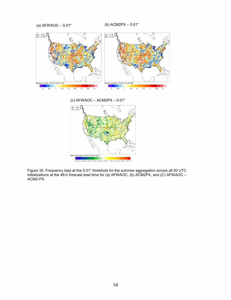
58

Figure 30. Frequency bias at the 0.01” threshold for the summer aggregation across all 00 UTC initializations at the 48-h forecast lead time for (a) AFWAOC, (b) ACM2PX, and (C) AFWAOC – ACM2-PX.

(a) AFWAOC – 0.01" (b) ACM2PX – 0.01"

(c) AFWAOC – ACM2PX – 0.01"

59

Figure 31. Gilbert skill score at the 0.10” threshold for the summer aggregation across all 00 UTC initializations at the 48-h forecast lead time for (a) AFWAOC, (b) ACM2PX, and (C) AFWAOC – ACM2-PX.

(a) AFWAOC – 0.10" (b) ACM2PX – 0.10"

(c) AFWAOC – ACM2PX – 0.10"

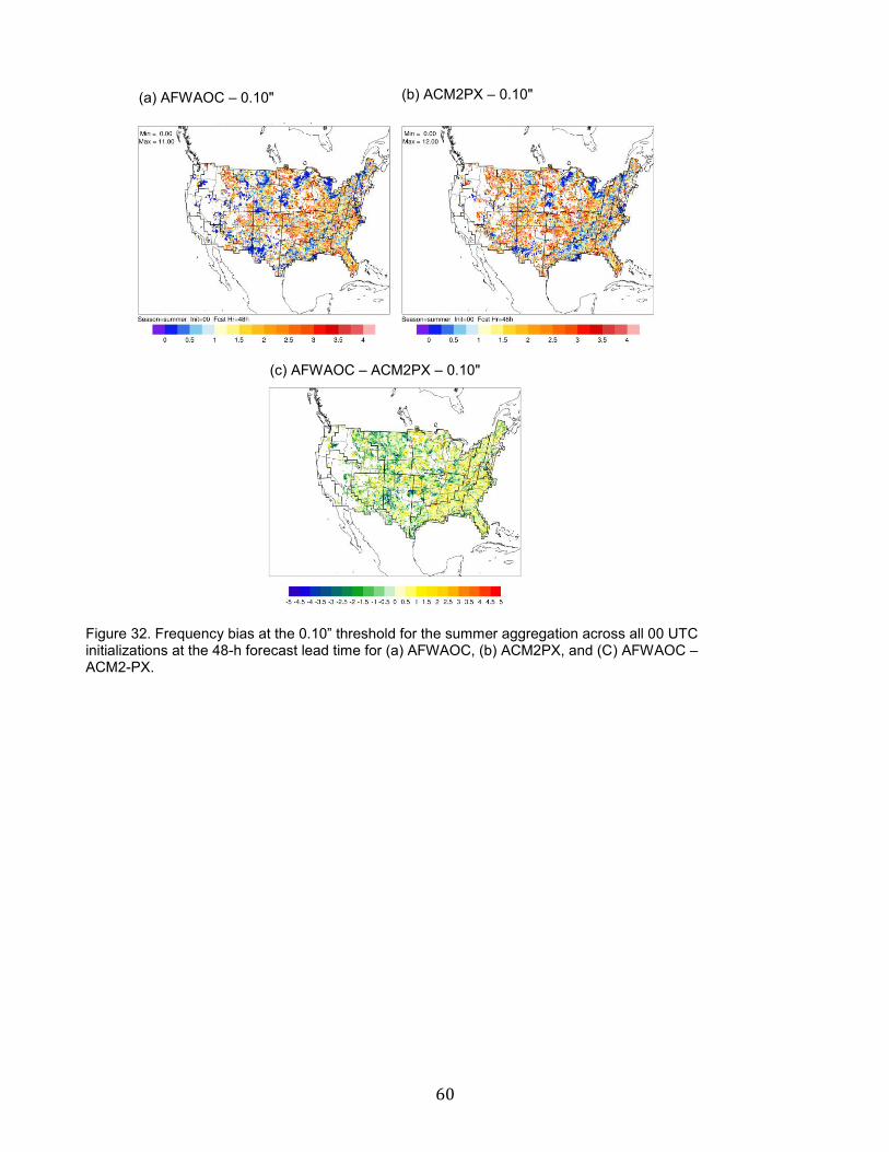
60

Figure 32. Frequency bias at the 0.10” threshold for the summer aggregation across all 00 UTC initializations at the 48-h forecast lead time for (a) AFWAOC, (b) ACM2PX, and (C) AFWAOC – ACM2-PX.

(a) AFWAOC – 0.10" (b) ACM2PX – 0.10"

(c) AFWAOC – ACM2PX – 0.10"

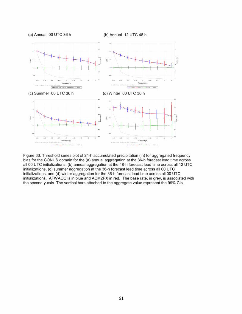
61

Figure 33. Threshold series plot of 24-h accumulated precipitation (in) for aggregated frequency bias for the CONUS domain for the (a) annual aggregation at the 36-h forecast lead time across all 00 UTC initializations, (b) annual aggregation at the 48-h forecast lead time across all 12 UTC initializations, (c) summer aggregation at the 36-h forecast lead time across all 00 UTC initializations, and (d) winter aggregation for the 36-h forecast lead time across all 00 UTC initializations. AFWAOC is in blue and ACM2PX in red. The base rate, in grey, is associated with the second y-axis. The vertical bars attached to the aggregate value represent the 99% CIs.

(a) Annual 00 UTC 36 h (b) Annual 12 UTC 48 h

(d) Winter 00 UTC 36 h (c) Summer 00 UTC 36 h

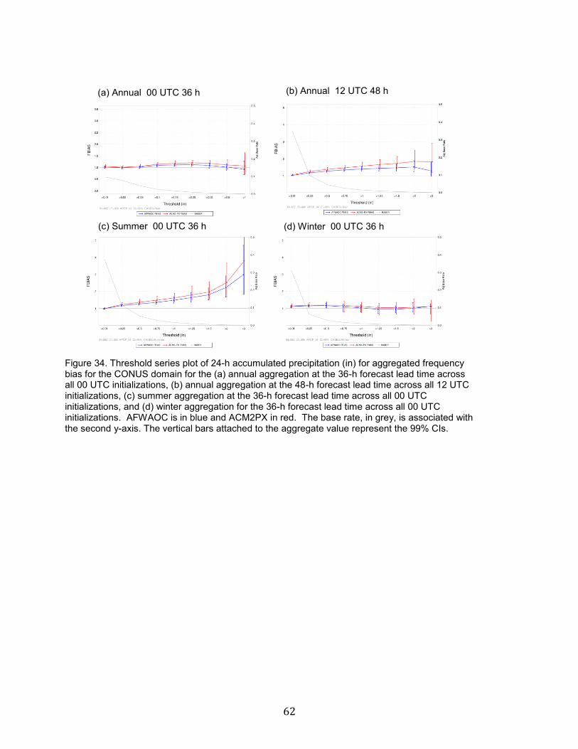
62

Figure 34. Threshold series plot of 24-h accumulated precipitation (in) for aggregated frequency bias for the CONUS domain for the (a) annual aggregation at the 36-h forecast lead time across all 00 UTC initializations, (b) annual aggregation at the 48-h forecast lead time across all 12 UTC initializations, (c) summer aggregation at the 36-h forecast lead time across all 00 UTC initializations, and (d) winter aggregation for the 36-h forecast lead time across all 00 UTC initializations. AFWAOC is in blue and ACM2PX in red. The base rate, in grey, is associated with the second y-axis. The vertical bars attached to the aggregate value represent the 99% CIs.

(a) Annual 00 UTC 36 h (b) Annual 12 UTC 48 h

(d) Winter 00 UTC 36 h (c) Summer 00 UTC 36 h

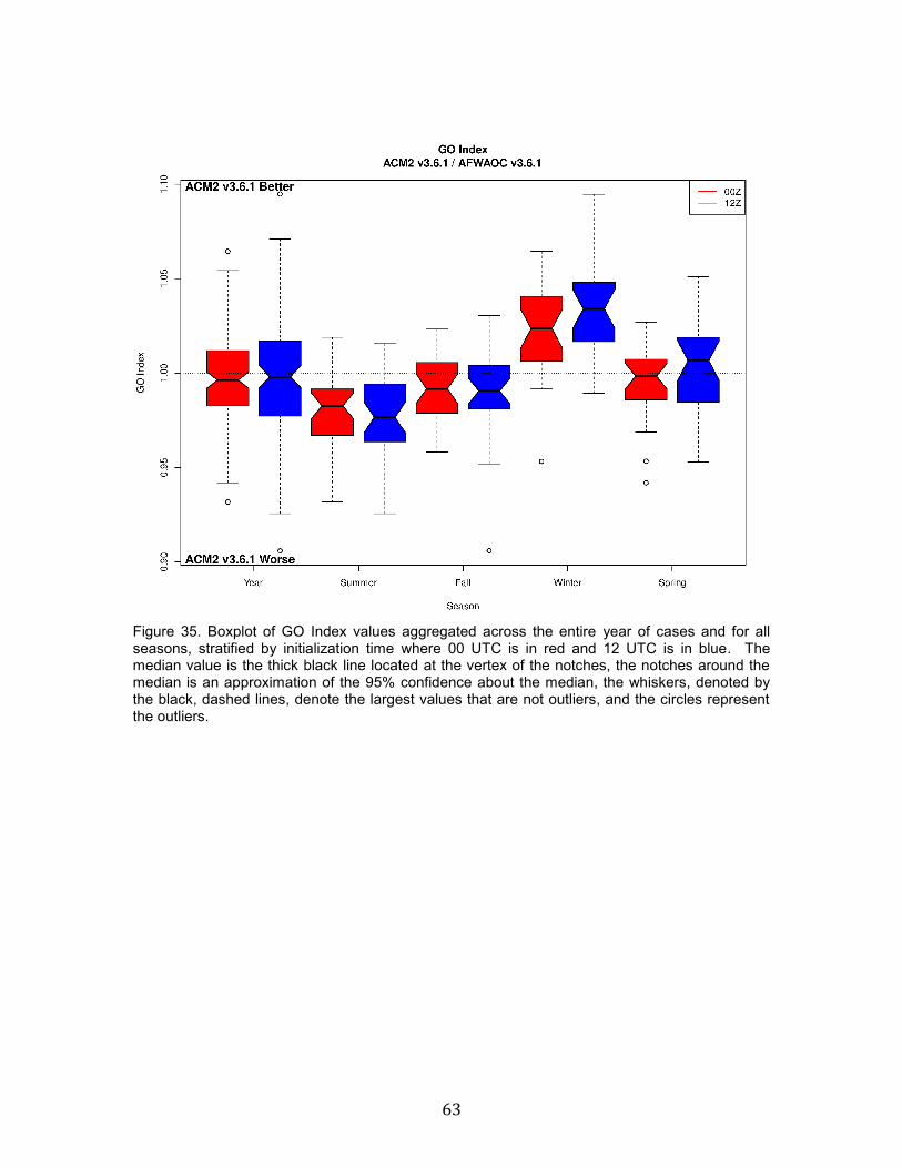
63

Figure 35. Boxplot of GO Index values aggregated across the entire year of cases and for all seasons, stratified by initialization time where 00 UTC is in red and 12 UTC is in blue. The median value is the thick black line located at the vertex of the notches, the notches around the median is an approximation of the 95% confidence about the median, the whiskers, denoted by the black, dashed lines, denote the largest values that are not outliers, and the circles represent the outliers.

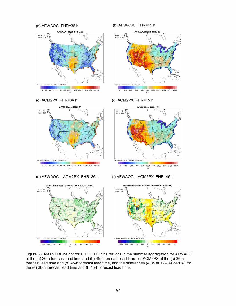
64

Figure 36. Mean PBL height for all 00 UTC initializations in the summer aggregation for AFWAOC at the (a) 36-h forecast lead time and (b) 45-h forecast lead time, for ACM2PX at the (c) 36-h forecast lead time and (d) 45-h forecast lead time, and the differences (AFWAOC – ACM2PX) for the (e) 36-h forecast lead time and (f) 45-h forecast lead time.

(a) AFWAOC FHR=36 h (b) AFWAOC FHR=45 h

(d) ACM2PX FHR=45 h (c) ACM2PX FHR=36 h

(f) AFWAOC – ACM2PX FHR=45 h (e) AFWAOC – ACM2PX FHR=36 h

65

Figure 37. Mean PBL height for all 00 UTC initializations in the winter aggregation for AFWAOC at the (a) 36-h forecast lead time and (b) 45-h forecast lead time, for ACM2PX at the (c) 36-h forecast lead time and (d) 45-h forecast lead time, and the differences (AFWAOC – ACM2PX) for the (e) 36-h forecast lead time and (f) 45-h forecast lead time.

(a) AFWAOC FHR=36 h (b) AFWAOC FHR=45 h

(d) ACM2PX FHR=45 h (c) ACM2PX FHR=36 h

(f) AFWAOC – ACM2PX FHR=45 h (e) AFWAOC – ACM2PX FHR=36 h

66

Figure 38. Mean differences (AFWAOC – ACM2PX) for latent heat flux (W m2) for all 00 UTC initializations at the 45-h forecast lead time for (a) fall, (b) winter, (c) spring, and (d) summer.

(a) Fall FHR=45 h (b) Winter FHR=45 h

(d) Summer FHR=45 h (c) Spring FHR=45 h

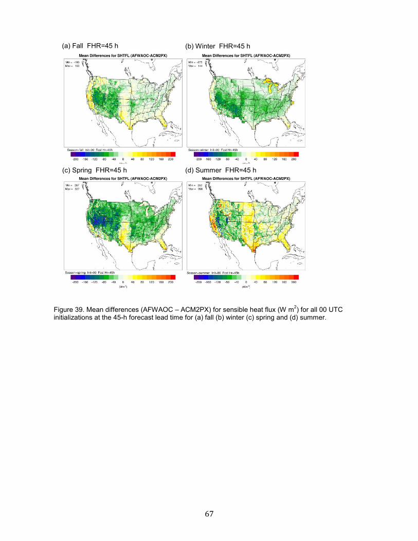
67

Figure 39. Mean differences (AFWAOC – ACM2PX) for sensible heat flux (W m2) for all 00 UTC initializations at the 45-h forecast lead time for (a) fall (b) winter (c) spring and (d) summer.

(a) Fall FHR=45 h (b) Winter FHR=45 h

(d) Summer FHR=45 h (c) Spring FHR=45 h

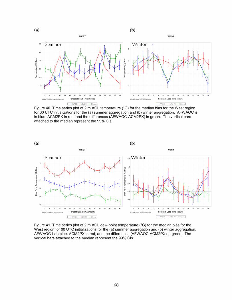
68

(a) (b)

Figure 40. Time series plot of 2 m AGL temperature (°C) for the median bias for the West region for 00 UTC initializations for the (a) summer aggregation and (b) winter aggregation. AFWAOC is in blue, ACM2PX in red, and the differences (AFWAOC-ACM2PX) in green. The vertical bars attached to the median represent the 99% CIs.

(a) (b)

Figure 41. Time series plot of 2 m AGL dew-point temperature (°C) for the median bias for the West region for 00 UTC initializations for the (a) summer aggregation and (b) winter aggregation. AFWAOC is in blue, ACM2PX in red, and the differences (AFWAOC-ACM2PX) in green. The vertical bars attached to the median represent the 99% CIs.

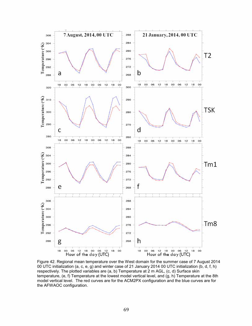
69

Figure 42. Regional mean temperature over the West domain for the summer case of 7 August 2014 00 UTC initialization (a, c, e, g) and winter case of 21 January 2014 00 UTC initialization (b, d, f, h) respectively. The plotted variables are (a, b) Temperature at 2 m AGL, (c, d) Surface skin temperature, (e, f) Temperature at the lowest model vertical level, and (g, h) Temperature at the 8th model vertical level. The red curves are for the ACM2PX configuration and the blue curves are for the AFWAOC configuration.

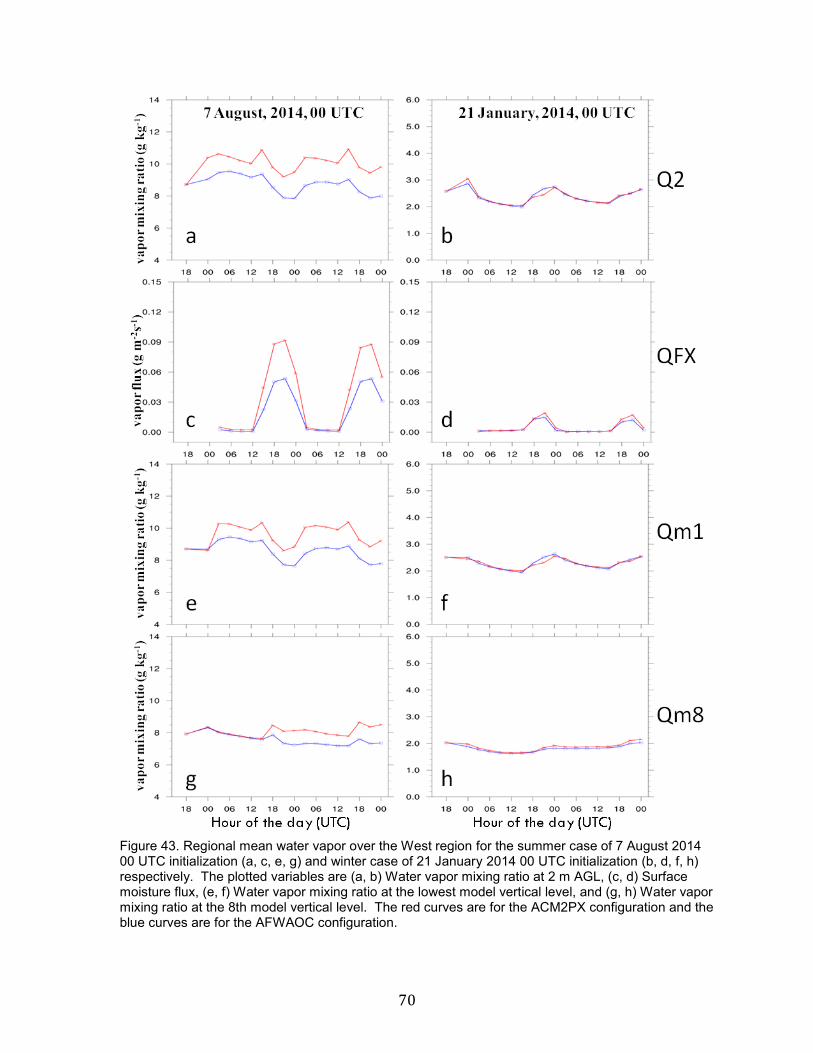
70

Figure 43. Regional mean water vapor over the West region for the summer case of 7 August 2014 00 UTC initialization (a, c, e, g) and winter case of 21 January 2014 00 UTC initialization (b, d, f, h) respectively. The plotted variables are (a, b) Water vapor mixing ratio at 2 m AGL, (c, d) Surface moisture flux, (e, f) Water vapor mixing ratio at the lowest model vertical level, and (g, h) Water vapor mixing ratio at the 8th model vertical level. The red curves are for the ACM2PX configuration and the blue curves are for the AFWAOC configuration.

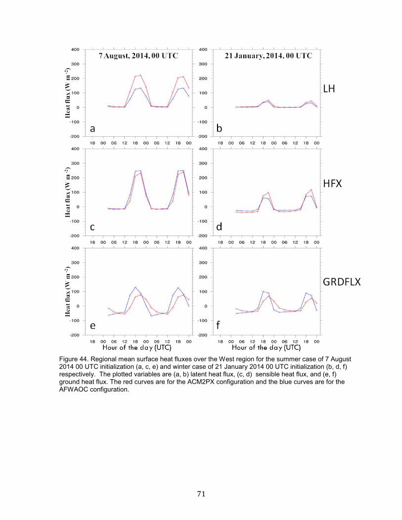
71

Figure 44. Regional mean surface heat fluxes over the West region for the summer case of 7 August 2014 00 UTC initialization (a, c, e) and winter case of 21 January 2014 00 UTC initialization (b, d, f) respectively. The plotted variables are (a, b) latent heat flux, (c, d) sensible heat flux, and (e, f) ground heat flux. The red curves are for the ACM2PX configuration and the blue curves are for the AFWAOC configuration.

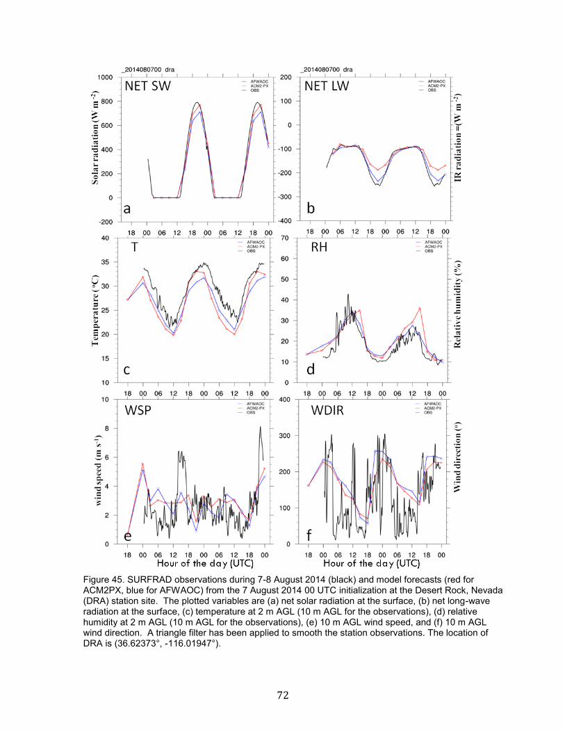
72

Figure 45. SURFRAD observations during 7-8 August 2014 (black) and model forecasts (red for ACM2PX, blue for AFWAOC) from the 7 August 2014 00 UTC initialization at the Desert Rock, Nevada (DRA) station site. The plotted variables are (a) net solar radiation at the surface, (b) net long-wave radiation at the surface, (c) temperature at 2 m AGL (10 m AGL for the observations), (d) relative humidity at 2 m AGL (10 m AGL for the observations), (e) 10 m AGL wind speed, and (f) 10 m AGL wind direction. A triangle filter has been applied to smooth the station observations. The location of DRA is (36.62373°, -116.01947°).

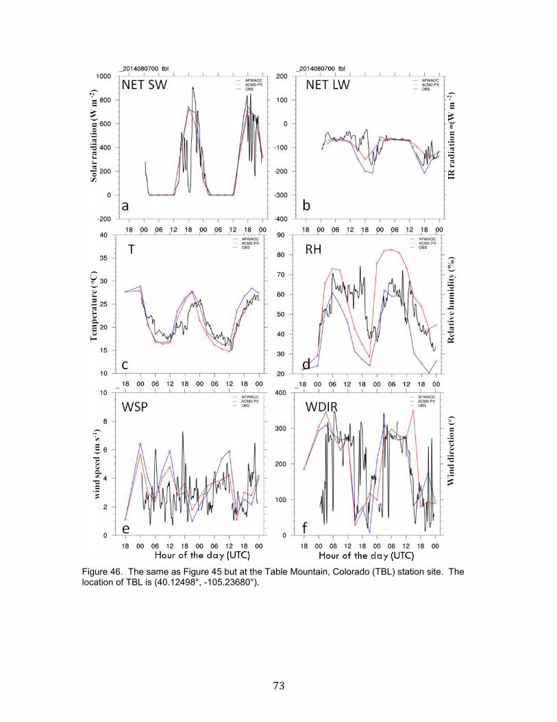
73

Figure 46. The same as Figure 45 but at the Table Mountain, Colorado (TBL) station site. The location of TBL is (40.12498°, -105.23680°).

74

Figure 47. The same as Figure 45 but at the Bondville, Illinois (BON) station site. The location of BON is (40.05192°, -88.37309°).

75

Appendix A: Case list.

00 UTC Initialization 12 UTC Initialization August 2013: 3, 6, 9, 12, 15, 18, 21, 24, 27, 30 August 2013: 1, 4, 7, 10, 13, 16, 19, 22, 25, 28, 31

September 2013: 2, 5, 8, 11, 14, 17, 20, 23, 26, 29 September 2013: 3, 6, 9, 12, 15, 18, 21, 24, 27, 30

October 2013: 2, 5, 8, 11, 14, 17, 20, 23, 26, 29 October 2013: 3, 6, 9, 12, 15, 18, 21, 24, 27, 30

November 2013: 1, 4, 7, 10, 13, 16, 19, 22, 25, 28 November 2013: 2, 5, 8, 11, 14, 17, 20, 23, 26, 29

December 2013: 1, 4, 7, 10, 13, 16, 19, 22, 25, 28, 31 December 2013: 2, 5, 8, 11, 14, 17, 20, 23, 26, 29

January 2014: 3, 6, 9, 12, 15, 18, 21, 24, 27, 30 January 2014: 1, 4, 7, 10, 13, 16, 19, 22, 25, 28, 31

February 2014: 2, 5, 8, 11, 14, 17, 20, 23, 26 February 2014: 3, 6, 9, 12, 15, 18, 21, 24, 27

March 2014: 1, 4, 7, 10, 13, 16, 19, 22, 25, 28, 31 March 2014: 2, 5, 8, 11, 14, 17, 20, 23, 26, 29

April 2014: 3, 6, 9, 12, 15, 18, 21, 24, 27, 30 April 2014: 1, 4, 7, 10, 13, 16, 19, 22, 25, 28

May 2014: 3, 6, 9, 12, 15, 18, 21, 24, 27, 30 May 2014: 1, 4, 7, 10, 13, 16, 19, 22, 25, 28, 31

June 2014: 2, 5, 8, 11, 14, 17, 20, 23, 26, 29 June 2014: 3, 6, 9, 12, 15, 18, 21, 24, 27, 30

July 2014: 2, 5, 8, 11, 14, 17, 20, 23, 26, 29 July 2014: 3, 6, 9, 12, 15, 18, 21, 24, 27, 30

August 2014: 1, 4, 7, 10, 13, 16, 19, 22, 25, 28, 31 August 2014: 2, 5, 8, 11, 14, 17, 20, 23, 26, 29

Appendix B: Example WRF namelist.input used in this test. &time_control run_days = 0, run_hours = 48, run_minutes = 0, run_seconds = 0, start_year = 2011, start_month = 07, start_day = 01, start_hour = 00, start_minute = 00, start_second = 00, end_year = 2012, end_month = 07, end_day = 03, end_hour = 00, end_minute = 00, end_second = 00, interval_seconds = 10800, history_interval = 180, frames_per_outfile = 1, restart = .false., io_form_history = 2, io_form_restart = 2, io_form_input = 2, io_form_boundary = 2, debug_level = 0, reset_simulation_start = .true., write_input = .false.,

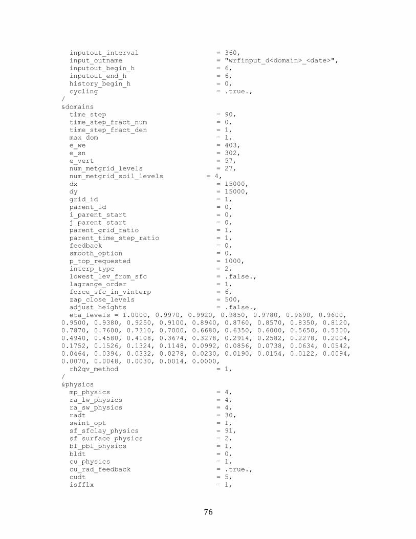
76

inputout_interval = 360, input_outname = "wrfinput_d<domain>_<date>", inputout_begin_h = 6, inputout_end_h = 6, history_begin_h = 0, cycling = .true., / &domains time_step = 90, time_step_fract_num = 0, time_step_fract_den = 1, max_dom = 1, e_we = 403, e_sn = 302, e_vert = 57, num_metgrid_levels = 27, num_metgrid_soil_levels = 4, dx = 15000, dy = 15000, grid_id = 1, parent_id = 0, i_parent_start = 0, j_parent_start = 0, parent_grid_ratio = 1, parent_time_step_ratio = 1, feedback = 0, smooth_option = 0, p_top_requested = 1000, interp_type = 2, lowest_lev_from_sfc = .false., lagrange_order = 1, force_sfc_in_vinterp = 6, zap_close_levels = 500, adjust_heights = .false., eta_levels = 1.0000, 0.9970, 0.9920, 0.9850, 0.9780, 0.9690, 0.9600, 0.9500, 0.9380, 0.9250, 0.9100, 0.8940, 0.8760, 0.8570, 0.8350, 0.8120, 0.7870, 0.7600, 0.7310, 0.7000, 0.6680, 0.6350, 0.6000, 0.5650, 0.5300, 0.4940, 0.4580, 0.4108, 0.3674, 0.3278, 0.2914, 0.2582, 0.2278, 0.2004, 0.1752, 0.1526, 0.1324, 0.1148, 0.0992, 0.0856, 0.0738, 0.0634, 0.0542, 0.0464, 0.0394, 0.0332, 0.0278, 0.0230, 0.0190, 0.0154, 0.0122, 0.0094, 0.0070, 0.0048, 0.0030, 0.0014, 0.0000, rh2qv_method = 1, / &physics mp_physics = 4, ra_lw_physics = 4, ra_sw_physics = 4, radt = 30, swint_opt = 1, sf_sfclay_physics = 91, sf_surface_physics = 2, bl_pbl_physics = 1, bldt = 0, cu_physics = 1, cu_rad_feedback = .true., cudt = 5, isfflx = 1,

77

ifsnow = 0, icloud = 1, surface_input_source = 1, num_soil_layers = 4, maxiens = 1, maxens = 3, maxens2 = 3, maxens3 = 16, ensdim = 144, mp_zero_out = 2, num_land_cat = 28, fractional_seaice = 1, seaice_threshold = 0.0, tice2tsk_if2cold = .true., / &dynamics rk_ord = 3, diff_6th_opt = 2, diff_6th_factor = 0.10, w_damping = 1, diff_opt = 1, km_opt = 4, damp_opt = 3, base_temp = 291., zdamp = 5000., dampcoef = 0.05, khdif = 0, kvdif = 0, smdiv = 0.1, emdiv = 0.01, epssm = 0.5, non_hydrostatic = .true., time_step_sound = 0, h_mom_adv_order = 5, v_mom_adv_order = 3, h_sca_adv_order = 5, v_sca_adv_order = 3, moist_adv_opt = 1, scalar_adv_opt = 0, chem_adv_opt = 0, tke_adv_opt = 0, use_baseparam_fr_nml = .true., / &bdy_control spec_bdy_width = 5, spec_zone = 1, relax_zone = 4, specified = .true., periodic_x = .false., symmetric_xs = .false., symmetric_xe = .false., open_xs = .false., open_xe = .false., periodic_y = .false., symmetric_ys = .false., symmetric_ye = .false., open_ys = .false.,

78

open_ye = .false., nested = .false., /