Embed Size (px)
Citation preview
The devil is in the tails: actuarial mathematics and the
subprime mortgage crisis
Catherine Donnelly and Paul Embrechts∗
RiskLab, ETH Zurich, Switzerland
January 4, 2010
Abstract
In the aftermath of the 2007-2008 financial crisis, there has been criticism of mathematicsand the mathematical models used by the finance industry. We answer these criticismsthrough a discussion of some of the actuarial models used in the pricing of credit derivatives.As an example, we focus in particular on the Gaussian copula model and its drawbacks. Toput this discussion into its proper context, we give a synopsis of the financial crisis and abrief introduction to some of the common credit derivatives and highlight the difficulties invaluing some of them.
We also take a closer look at the risk management issues in part of insurance industrythat came to light during the financial crisis. As a backdrop to this, we recount the eventsthat took place at American International Group during the financial crisis. Finally, throughour paper we hope to bring to the attention of a broad actuarial readership some “lessons(to be) learned” or “events not to be forgotten”.
1 Introduction
“Recipe for disaster: the formula that killed Wall Street”. That was the title of a web-articleSalmon (2009) that appeared in Wired Magazine on February 2009. It was shortly followed bya Financial Times article Jones (2009) called “Of couples and copulas: the formula that felledWall St”. Both articles were written about an actuarial model called the Li model which is usedin credit risk management. The impression gained is that an actuary developed a mathematicalmodel which subsequently caused the downfall of Wall Street banks.
Both articles attempt to explain the limitations of the model, and its role in the 2007-2008financial crisis (“the Crisis”). While the earlier article Salmon (2009) acknowledges that thedeficiencies of the model have been known for sometime, the later Financial Times article Jones(2009) asks why no-one noticed the model’s Achilles’ heel.
For some of us, the implication that a mathematical model shoulders much of the blame forthe difficulties on Wall Street and that few people were aware of its limitations are untenable.Indeed, we aim to demonstrate that such criticism is entirely unjustified.
Yet these criticisms of one particular model, with their unwarranted focus on the man whointroduced the model to the credit derivative world, fly within a barrage of accusations directedat financial mathematics and mathematicians. A typical example is to be found in the New
∗Senior SFI Chair
1
York Times of September 12, 2009: “Wall Street’s Math Wizards Forgot a Few Variables”; seeLohr (2009). Many more have been published. These accusations come not only from newspaperarticles such as those cited above, but even from government-instigated reports into the Crisis.Turner (2009) has a section entitled “Misplaced reliance on sophisticated maths”. An interestingreply to the Turner Review came from Professor Sir David Wallace, Chair of the Council forthe Mathematical Sciences, who on behalf of several professors of mathematics in the UK statesthat: “Another aspect on which we would welcome dialogue concerns the reference to a misplacedreliance on sophisticated maths and the possible interpretation that mathematics per se has anegative effect in the city. You can imagine that we strongly disagree with this interpretation!But of course the purpose of mathematical and statistical models must be better understood. Inparticular we believe that the FSA [Financial Services Authority] and the research communityshare an objective to enhance public appreciation of uncertainties in modelling future behaviour”;see Wallace (2009).
We believe that there should be a reliance on sophisticated mathematics. There has beentoo often a problem of misplaced reliance on unsophisticated mathematics or, in the words ofL.C.G. Rogers, “The problem is not that mathematics was used by the banking industry, theproblem was that it was abused by the banking industry. Quants were instructed to build modelswhich fitted the market prices. Now if the market prices were way out of line, the calibratedmodels would just faithfully reproduce those wacky values, and the bad prices get reinforced byan overlay of scientific respectability!”; see Rogers (2009). For an excellent article (written inGerman) taking a more in-depth look at the importance of mathematics for finance and its rolein the current crisis, see Follmer (2009). The main contributions from mathematics to economicsand finance are summarized in Follmer (2009) as follows:
• understanding and clarifying models used in economics;
• making heuristic methods mathematically precise;
• highlighting model conditions and restrictions on applicability;
• working out numerous explicit examples;
• leading the way for stress-testing and robustness properties, and
• offering a relevant and challenging field of research on its own.
We cannot answer every accusation directed at financial mathematics. Instead, we look at theLi model, also called the Gaussian copula model, and use it as a proxy for mathematics appliedbadly in finance. It should be abundantly clear that it is not mathematics that caused the Crisis.At worst, a misuse of mathematics, and we mean mathematics in a broad sense and not just oneformula, partly contributed to the Crisis.
The Gaussian copula model has been embraced enthusiastically by industry for its simplicity.While a simple model is to be preferred to a complex one, especially in a financial world whichcan only be partially and imperfectly described by mathematics, we believe that the model istoo simple. It does not capture the main features of what it is attempting to model. Yet itwas, and still is, applied to the credit derivatives which played a major part in the Crisis. Wedevote a large part of this article to explaining the Gaussian copula model and examining itsshortcomings.
We also rebutt the claim that few people saw the flaws underlying several of the quantitativetechniques used in the pricing and risk management of credit derivatives. On the contrary, manyacademics and practitioners were aware of them and on numerous occasions exposed these flaws.
2
As the fields of insurance and finance increasingly overlap, it is maybe not surprising thatone casualty of the Crisis was an insurance company, American Insurance Group (“AIG”). Withinsurance companies selling credit default swaps, which have insurance-like features, and catas-trophe bonds and mortality bonds, which are a way of selling insurance risk in the financialmarket, it is an opportune time to examine what caused the near-collapse of AIG. We ask whatlessons other insurance companies and those involved in running them, such as actuaries andother risk professionals, can learn from the AIG story.
It is also a good time to pause and think about our roles and responsibilities in the financeindustry. Are the practitioners truly aware of the assumptions, whether implicit or explicit, inthe mathematics they use? If not, then they have a duty to inform themselves. It is also theduty of the academics who are publishing articles not only to make their assumptions explicitbut also, upon use, to communicate their assumptions more forcefully to the end-user.
Before we delve into the above, we begin by outlining the Crisis.
2 The roots of the subprime mortgage crisis
The Crisis was complex and of global proportions. There will undoubtedly be a multitude ofarticles and books penned about it for years to come. Among currently available, more academic,excellent analyses are Brunnermeier (2009), Crouhy et al. (2008) and Hellwig (2009). We alsohighly recommend The Economist (2008). As our focus is on some of the mathematical andactuarial issues which arose from the Crisis, we relate only the story of the Crisis which isrelevant for this article.
The root of the Crisis was the transfer of the risk of mortgage default from mortgage lenders tothe financial market at large: banks, hedge funds, insurance companies. The transfer was effectedby a process called securitization. The practical mechanics of this process can be complicated,as institutions seek to reduce costs and tax-implications. However, the essence of what is doneis as follows.
A bank pools together mortgages which have been taken out by residential home-ownersand commerical property organizations. The pool of mortgages is transferred to an off-balance-sheet trust called a special-purpose vehicle (“SPV”). While sponsored by the bank, the SPV isbankruptcy-remote from it. This means that a default by the bank does not result in a default bythe SPV. The SPV issues coupon-bearing financial securities called mortgage-backed securities.The mortgage repayments made by the home-owners and commerical property organizations aredirected towards the SPV, rather than being received by the bank which granted the mortgages.After deducting expenses, the SPV uses the mortgage repayments to pay the coupons on themortgage-backed securities. Typically, the buyers of the mortgage-backed securities are orga-nizations such as banks, insurance companies and hedge funds. This process allowed banks tomove from an “originate to hold” model, where they held the mortgages they made on theirbooks, to an “originate to distribute” model, where they essentially sold on the mortgages.
Not only mortgages can be securitized, but also other assets such as auto loans, student loansand credit card receivables. A security issued on fixed-income assets is called a collateralized debtobligation (“CDO”), and if the underlying assets of the CDO consist of loans then it is calleda collateralized loan obligation. However, the underlying assets do not have to be fixed-incomeassets and the general term for a security issued on any asset is an asset-backed security.
There is nothing inherently wrong with the securitization process. It is a transfer of risk fromone party to another, in this case the risk of mortgage default. It should increase the efficiency offinancial markets as it allows those who are happy to take on the risk of mortgage default to buyit. Moreover, as banks must hold capital against the loans on their books, selling most of the pool
3
of mortgages allows them to free up capital. The view on the benefits of securtization to overallfinancial stability in 2006 is summarized in the following quote from one of the IMF’s GlobalFinancial Stability Reports in that year: “There is a growing recognition that the dispersion ofcredit risk by banks to a broader and more diverse group of investors, rather than warehousingsuch risk on their balance sheets, has helped make the banking and overall financial system moreresilient. ... The improved resilience may be seen in fewer bank failures and more consistentcredit provision. Consequently, the commercial banks, ..., may be less vulnerable today to creditor economic shocks”; see IMF (2006, Chapter II). Indeed, this was the prevailing view until late2006. Yet the process of transferring one type of risk creates other types of risks.
As it turned out, the main additional risk in securitization was moral hazard. A lengthydiscussion of the role of moral hazard in the Crisis can be found in Hellwig (2009). For securitizedproducts, sources of moral hazard included:
• the failure of some originators of securitized products to retain any of the riskiest part ofthe CDO. We examine this point in the next paragraph;
• the credit rating agencies had a conflict of interest in that they were advising customers onhow to best securitize products and then credit rating those same products. SEC (2008)gives a flavor of the practices in the three main credit rating agencies leading up to theCrisis;
• the chain of financial intermediation from the originators to the buyers of some securitizedproducts may have been too long, resulting in opaqueness, a loss of information and anincreased scope for moral hazard (see also Subsection 6.2), and
• some financial institutions may have deemed themselves “too big too fail”, with a corre-sponding disregard for the level of risk they were exposed to and a belief on their part thatthe government would not allow them to fail since they were systematically too important.Wolf (2008) has a delightful phrase for this: “privatising gains and socialising losses”. Seealso anecdotal evidence from Haldane (2009b, page 12).
If a bank is not exposed to the risk of mortgage default, then it has no incentive to controland maintain the quality of the loans it makes. To protect against this, the theory was thatthe banks should retain the riskiest part of the mortgage pool. In practice, this did not alwayshappen, which led to a reduction in lending standards; see Keys et al. (2008). This possibility wasforeseen some fifteen years before the Crisis with remarkable prescience by Stiglitz, as he pointsout in Stiglitz (2008). Because of its prime importance in the current discussion of the Crisis,but also as it reflects indirectly on the possibility of bank-assurance products, we repeat someof its key statements, written in 1992: “...has the growth in securitization been a result of moreefficient transactions technologies, or an unfounded reduction in concern about the importanceof screening loan applicants? ... we should at least entertain the possibility that it is the latterrather than the former... At the very least, the banks have demonstrated an ignorance of two verybasic aspects of risk: (a) the importance of correlation,... (b) the possibility of price declines.”
As the quality of the mortgages granted declined, the risk characteristics of the underlyingpool of mortgages changed. In particular, the risk of mortgage default increased. It appearsthat many market participants either did not realize this was happening or did not think that itwas significant. In February 2007, an increase in subprime mortgage defaults was noted, and theCrisis started unfolding. There were many factors which contributed strongly to the Crisis, suchas fair-value accounting, systemic interdependence, a move by banks to financing their assetswith shorter maturity instruments, which left them vulnerable to liquidity drying-up, and otherfactors, such as ratings agencies and an excessive emphasis on revenue and growth by financial
4
institutions. However, the reader should look elsewhere for an explanation of their impact, suchas in the references mentioned at the start of this section.
3 Securitization
Securitization is the process of pooling together financial assets, such as mortgages and autoloans, and redirecting their cashflows to support coupon payments on CDOs. Here we describeCDOs in more detail.
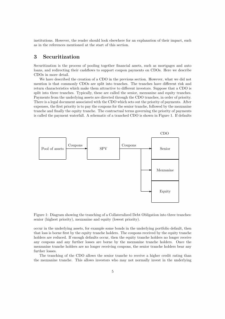
We have described the creation of a CDO in the previous section. However, what we did notmention is that commonly CDOs are split into tranches. The tranches have different risk andreturn characteristics which make them attractive to different investors. Suppose that a CDO issplit into three tranches. Typically, these are called the senior, mezzanine and equity tranches.Payments from the underlying assets are directed through the CDO tranches, in order of priority.There is a legal document associated with the CDO which sets out the priority of payments. Afterexpenses, the first priority is to pay the coupons for the senior tranche, followed by the mezzaninetranche and finally the equity tranche. The contractual terms governing the priority of paymentsis called the payment waterfall. A schematic of a tranched CDO is shown in Figure 1. If defaults
Pool of assets -Coupons
SPV -Coupons
-
-
Senior
Mezzanine
Equity
CDO
Figure 1: Diagram showing the tranching of a Collateralized Debt Obligation into three tranches:senior (highest priority), mezzanine and equity (lowest priority).
occur in the underlying assets, for example some bonds in the underlying portfolio default, thenthat loss is borne first by the equity tranche holders. The coupons received by the equity trancheholders are reduced. If enough defaults occur, then the equity tranche holders no longer receiveany coupons and any further losses are borne by the mezzanine tranche holders. Once themezzanine tranche holders are no longer receiving coupons, the senior tranche holders bear anyfurther losses.
The tranching of the CDO allows the senior tranche to receive a higher credit rating thanthe mezzanine tranche. This allows investors who may not normally invest in the underlying
5
assets to invest indirectly in them, through the CDO. For example, suppose the underlying poolof assets has an aggregate credit rating of BBB. Before tranching, the credit rating of the CDOwould also be BBB. However, with judicious tranching, the senior tranche can achieve a AAAcredit rating. This is because it is exposed to a much reduced risk of default from the underlyingassets, since any losses arising from default in the underlying portfolio are borne first by theequity tranche holders and then the mezzanine tranche holders. Usually, the mezzanine trancheis BBB-rated and the equity tranche is not credit rated.
The SPV aims to maximize the size of the senior tranche, subject to it attaining a AAAcredit-rating. The maximization of the size of the senior tranche may mean that it is just withinthe boundary of what constitutes a AAA-rated investment. Typically, the senior tranche is wortharound 80% of the nominal value of the underlying portfolio of assets. This means that 20%of the underlying portfolio must default before the holders of the senior tranche of the CDOhave their coupon payments reduced. Similarly, the SPV maximizes the size of the mezzaninetranche, subject to it attaining a BBB credit-rating. Typically, the mezzanine tranche is worthin the region of 15% of the nominal value of the underlying portfolio of assets. This means that5% of the underlying portfolio must default before the holders of the mezzanine tranche of theCDO have their coupon payments reduced. The remaining part of the CDO is allocated to theequity tranche, which is unrated and is worth the remaining 5% nominal value of the underlyingportfolio of assets. As the equity tranche has the lowest priority in payments, any defaults inthe underlying portfolio of assets reduce the coupon payments of the equity tranche holders.
The key to valuing CDOs is modeling the defaults in the underlying portfolios. It is clear fromthe description above that the coupon payments received by the holders of the CDO tranchesdepend directly on the defaults occurring in the underlying portfolio of assets. As Duffie (2008)points out, the modeling of default correlation is currently the weakest link in the risk measure-ment and pricing of CDOs. There are several methods of approaching the valuation of a CDO, afew of which we mention briefly in Section 7, but first we clear the stage and allow the Gaussiancopula to enter.
4 The Gaussian copula model
On March 27 1999, the second author gave a talk at the Columbia-JAFEE Conference on theMathematics of Finance at Columbia University, New York. Its title was “Insurance Analytics:Actuarial Tools in Financial Risk-Management” and it was based on a 1998 RiskLab report thathe co-authored with Alexander McNeil and Daniel Straumann; see Embrechts et al. (2002). Themain emphasis of the report was on explaining to the world of risk management the variousrisk management pitfalls surrounding the notion of linear correlation. The concept of copula,by now omnipresent, was only mentioned in passing in Embrechts et al. (2002). However, itsappearance in Embrechts et al. (2002) started an avalanche of copula-driven research; see Genestet al. (2009). During the coffee break, David Li walked up to the second author, saying thathe had started using copula-type ideas and techniques, but now wanted to apply them to newlyinvented credit derivatives like CDOs. The well-known paper Li (2000) was published one yearlater. In it is outlined a copula-based approach to modeling the defaults in the underlying pool.Suppose we wish to value a CDO which has d bonds in the underlying portfolio. As we mentionedin the previous section, we can do this if we can find the joint default distribution of the d bonds.Denote by Ti the time until default of the ith bond, for i = 1, . . . , d. How can we determine thedistribution of the joint default time, P[T1 ≤ t1, . . . , Td ≤ td]? If we can do this, then we have away to value the CDO.
6
4.1 A brief introduction to copulas
Using copulas allows us to separate the individual behaviour of the marginal distributions fromtheir joint dependency on each other. We focus only on the copula theory that is necessary forthis article. An introduction to copulas can be found in Nelsen (2006) and a source of some ofthe more important references on the theory of copulas can be found in Embrechts (2009).
Consider two random variables X and Y defined on some common probability space. Forexample, the random variables X and Y could represent the times until default of two companies.What if we wish to specify the joint distribution of X and Y , that is to specify the distributionfunction (“df”) H(x, y) := P[X ≤ x, Y ≤ y]? If we know the individual dfs of X and Y then wecan do this using a copula. A copula specifies a dependency structure between X and Y , that ishow X and Y behave jointly.
More formally, a copula is defined as follows.
Definition 4.1. A d-dimensional copula C : [0, 1]d → [0, 1] is a df with standard uniformmarginal distributions.
An example of a copula is the independence copula C⊥, defined in two-dimensions as
C⊥(u, v) := uv, ∀u, v ∈ [0, 1].
It can be easily checked that C⊥ satisfies Definition 4.1. We can choose from a variety ofcopulas to determine the joint distribution. Which copula we choose depends on what type ofdependency structure we want. The next theorem tells us how the joint distribution is formedfrom the copula and the marginal dfs. It is the easy part of Sklar’s Theorem and the proof canbe found in Schweizer and Sklar (1983, Theorem 6.2.4).
Theorem 4.2. Let C be a copula and F1, . . . , Fd be univariate dfs. Defining
H(x1, . . . , xd) := C (F1(x1), . . . , Fd(xd)) , ∀(x1, . . . , xd) ∈ Rd,
the function H is a joint df with margins F1, . . . , Fd.
4.2 Two illustrative copulas
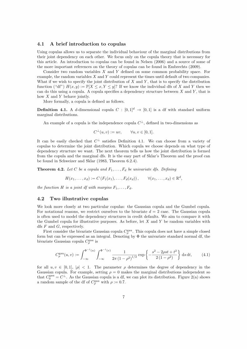
We look more closely at two particular copulas: the Gaussian copula and the Gumbel copula.For notational reasons, we restrict ourselves to the bivariate d = 2 case. The Gaussian copulais often used to model the dependency structures in credit defaults. We aim to compare it withthe Gumbel copula for illustrative purposes. As before, let X and Y be random variables withdfs F and G, respectively.
First consider the bivariate Gaussian copula Cgauρ . This copula does not have a simple closed
form but can be expressed as an integral. Denoting by Φ the univariate standard normal df, thebivariate Gaussian copula Cgau
ρ is
Cgauρ (u, v) :=
∫ Φ−1(u)
−∞
∫ Φ−1(v)
−∞
1
2π (1− ρ2)1/2
exp
{−s
2 − 2ρst+ t2
2 (1− ρ2)
}dsdt, (4.1)
for all u, v ∈ [0, 1], |ρ| < 1. The parameter ρ determines the degree of dependency in theGaussian copula. For example, setting ρ = 0 makes the marginal distributions independent sothat Cgau
0 = C⊥. As the Gaussian copula is a df, we can plot its distribution. Figure 2(a) showsa random sample of the df of Cgau
ρ with ρ := 0.7.
7
●
●
●
●
●
●
●
●
●
●
●
●
●
●
●
●
●
●
●
●
●
●
●●
●
●
●
●
●
●
●
●
●
●
●
●
●
●
●
●
●
●
●●
●
●
●
●
●
●
●
●
●
●
●
●
●
●
●
●
●
●
●
●
●●
●
●
●
●
●
●●
●
●
●
●
●
●
●●
●
●
●
●
●
●
●
●
●
●
●
●●
●
●
●
●
●
●
●
●
●
●
●
●
●
●
●
●
●
●
●
●
●
●
●
●
●
●
●
●
●
●
●
●
●
●
●
●
●
●
●
●
●
●
●
●
●
●
●
●
●
●
●
●
●
●
●
●
●
●
●
●
●
●
●
●
●
●
●
●
●
●
● ●
●
●
●
●
●
●
●
●
●
●
●
●
●
●
●
●
●●
●
●
●
●
●
●
●
●
●
●
●
●
●
●●
●
●
●
●
●
●
●
●
●
●
●●●
●●
●
●
●
●
●
●
●●
●
●
●
●
●
●
●
●
●
●
●
●
●
●
●
●
●
●
●
●
●
●●
●
●
●●
●
●
●
●
●
●
● ●
●
●
●
●
●
●
●
●
●
●
●
●
●
●
●
●
●
●
●
●
●
●
●
●
●
●
●
●
●
●●
●●
●
● ●
●
●
●
●
●
●
●
●
●
●
●
●
●
●
●
●
●
●
●
●
●
●
●
●
●
●
●
●
●
●
●
●
●●
●
●
●
●
●
●
●
●
●
●
●
●
●●
●
●
● ●
●
●
●
●
●●
●
●
●
●
● ●
●
●
●
●
●
●
●
●
●
●
●
●
●
●
●
●
●
●●
●
●
●
●
●
●
●
●
●
●
●
●
●
●
●
●
●
●
●
●
●
●
●
●●
●
●
●
●
●
● ●
●
●
●
●
●
●
●
●
●
●
●
●
●
●
●
●
●●
●
●
●
●
●
●
●
●
●
●
●
●
●
●
●
●
●
●
●
●
●
●
●
● ●● ●
●
●
●
●
●
●
●
●
●
●
●
●
●
●
●
●
●
●
●
●
●
●
●
●
●
●
●
●
●
●
●
●
●
●●
●
●
●
●
●●
●
●
●
●
●
●
●
●
●
●
●
●
●
●
●
●
●
●
●
●
●
●
●
●
●
●
●
●
●
●●
●
●
●
●
●
●
●
●
●●●
●
●
●
●
●
●
●
●
●
●
●
●
●
●●
●
●
●
●
●
●
●
●
●
●
●
●
●
●
●
●
●
●
●
●
●
●
●
●
●
●
●
●
●
●
●
●
●
●
●
●
●
●
●
●
●
●
●
●
●
●
●
●●
●
●
●
●
●
●
●
●●
●
●
●●
●
●
●
●
●
●
● ●
●
●
●
●
●
●
●
●
●
●
●
●
●
●
● ●
●
●
●
●
●
●
●
●
●
●
●●
●
●
●
●
●
●
●
●
●
●
●
●
●
●
●
●
●
●
●
●
●
●
●
●
●
●
●
●
●
●
●
●
●
●
●●
●
●
●
●
●
●
●
●●
●
●
●
●
●
●
●
●●
●
●●●
●
●
●
●
●
●
●
●
●
●
●
●
●
●
●
●
●
●
●
●
●
●
●
●
●
●
●
●
●
●
●
●
●
●
●
●●
●
●
●
●
●
●
●
●
●
●
●
●
●
●
●
●
●
●
●
●
●
●
●
●
●
●
● ●
●
●
●
●
●
●
●
●
●
●●
●●
●
●
●
●
●
●
●
●
●●
●
●
●●
●
●
●
●
●
●
●
●
●
●
●
●
●
●
●
●
●
●
●
●
●
●
●
●
●
●
●
●
●
●
●
●
●
●
●
●
●
●
●
●
●
●
●
●
●
●
●
●
●
●●
●
●
● ●
●
●
●
●
●
●
●
●
●
●
●
●
●
●
●
●
●
●
●
● ●
●
●
●
●
●
●
●
●
●
●
●
●
●
●
●
●
●
●
●●
●
●
●
●
●
●
●
●
●●
●
●
●
●
●
●
●
●
●
●
●
●
●
●
●
●
●
●
●
●
●
●●
●
●
●●
●
●
●
●
●
●
●
●
●
●
●
●
●
●
●
●
●
●
●
●
●
●
●
● ● ●
●
●
●
●
●●
●
●
●
●
●
●
●
●
●
●
●
●
●
●
●
●
●
●
●
●
●
●
● ●
●
●
●
●
●
●
●
●
●
●
●●
●
●
●
●
●
●
●
●
●
●
●
●
●
●
●
●
●
●
●
●
●●
●
●
●
●
●
●
●●
●
●
●
●
●
●
●
●
●
●
●
●
●●
●
●
●
●
●
●●
●
●
●
●
●
●
●
●
●
●
●●
●
●
●
●
●
●
●
●
●
●
●
●
●
●
●
●
●
●
●
●
●
●
●
●
●
●
●
●
●
●
●
●
●
●
●
●●
●
●●
●
●
●
●
●
●
●
●
●
●
●
●
●
●
●
●
●
●●
●
●●
●
●●
●
●
●
●
●
●
●
●
●
●
●
●
●
●
●
●
●
●
●
●
●
●
●
●
●
●
●
●
●
●
●
●
●
●
●
●
●
●
●
●
●●
●
●
●
●
●
●
● ●
●
●
●
●
●
●
●
●
●
●
●
●
●
●
●
●
●
●
●
●
●
●
●
●
●
●
●
●
●
●
●
●
●
●
●
●
●
●
●
●
●
●
●
●
●
●
●
●
●
●
●
●
●
●
●
●
●●
●
●
●
●
●
●
●
●
●
●
●
●
●
●
●
●
●
●
●
●
●
●
●
●
●
●
●
●
●
●
●
●
●
●
●
●
●
●
●
●
●
●
●
●
●
●
●
●
●
●
●
●
●
●
●
●
●
●
●
●
●
●
●
●
●●
●
●
●
●
●
●
●
●
●
●
●
●
●
●
●
●
●
●
●
●
● ●
●●
●
●
●
●
●
●
●
●
●
●
●
●
●
●
●
●
●
●
●
●
●
●
●
●
●
●
●
●
●
●
●
● ●
●
●
●
●
●
●
●
●
●
●
●
●
●
●
●
●
●
●
●
●
●
●
●
●
●
●
●
●
●
●
●
●
●
●
●
●
●
●
●
●
●
●
●
●
●
●
●
●
●
●
●
●
●
●
●
●
●
●
●
●
●
●
●
●
●
●
●
●
●
●
●
●
●
●
●
●
●
●
●
●
●
●
●
●
●
●
●
●
●
●
●●
●
●
●
●
●
●
●
●
●
●●
●
●
● ●
●
●
●
●
●
●
●
●
●
●
●
● ●
●
●
● ●
●
●
●
●
●
●
●
●
●
●
●
●
●
●
●
●
●
●
●
●
●●
●
●
●
●
●
●
●
●
●
●
●
●
●
●
●
●
●
●
●●
●
●
●
●
●
●
●
●
●
●
●
●
●
●
●
●
●
●
●
●
●
●
●
●
●●
●
●●
●
●
●
●
●
●
●
●
●
●
●
●
●
●
●
●●
●
●
●
●
●
●
●
●
●
●
●
●
●
●
●
●
●
●
●
●
●
●
●
●
●●
●
●
●
●
●
●
●
●
●
●
●
●
●
●
●
●
●
●
●
●
●
●
●
●●
●
●
●
●
●
●
●
●●
●
●
●
●
●
●
●
●
●
●
●
●●
●
●
●
●
●
●
●
●
●
●
●
●
●
●●
●
●
●
●
●
●
●
●
●
●
●
●
●
●
●
●
●
●
●
●
●
●
●
●
●
●
●
●
●
●
●
●
●●
●
●
●
● ●
●●
●
●
●
●
●
●
●●
●
●
●
●
●
●
●
●
●
●
●
●
●
●
●
●
●
●
●
●
●
●
●
●
●
●
●
●
●
●
●
●
●
●
●
●
●
●
●
●
●
●
●
●
●
●
●
●
●
●
●
●
●
●
●
●
●
●
●
●
●
●
●
●
●
●
●
●
●
●
●
●
●
●
●
●
●
●
●
●
●
●
●
●
●
●
●
●
●
●
●
●
●
●
●
●
●
●
●
●
●
●
●
●
●
●
●
●
●
●
●
●
●
●
●
●
●
●
●
●
●
●
●
●
●
●
●
●
●
●
●
●
●
●
●
●
●
●
●
●●
●
●
●
●
●
●
●
●
●
●
●
●
●
●●
●
●
●
●
●
●
●
●
●
●
●
●
●
●
●
●
●
●
●
●
●
●
●
●
●
●
●
●●
●
●
●
●
●
●
●
●
●
●
●●
●
●
●●
●
●
●
●
●
●
●
●●
●
●
●
●
●
●
●
●
● ●
●
●
●
●
●
●
●
●
●
●
●
●
●
●
●
●
●
●●
●
●
●
●
●
●
●
●
●
●
●
●
●
●
●
●
●
●
●
●
●
●
●
●
●
●
●
●
●
●
●
●
●
●
●●
●
●
●
●
●
●
●
●
●
●
●
●
●
●
●
●
●
0.0 0.2 0.4 0.6 0.8 1.0
0.0
0.2
0.4
0.6
0.8
1.0
U
V
(a) Gaussian copula Cgauρ with ρ := 0.7.
●
●
●
●
●
●
●
●
●
●
●
●
●
●
●
●
●
●
●
●
●
●
●●
●
●
●
●
●
●
●
●
●
●
●
●
●
●
●
●
●
●
●
●
●
●
●
●
●
●
●
●
●
●
●
●
●
●
●
●
●
●
●
●
●
●
●
●
●
●
●
●
●
● ●
●●
●
●
●
●
●
●
●
●
●
●
●
●
●
●
●
●
●
●
●
●
●
●
●
●
●
●
●
●
●
●
●
●
●
●
●
●
●
●
●
●
●
●
●
●●
●
●
●
●
●
●
●
●
●
●
●
●
●
●
●
●
●
●
●
●
●
●
●
●
●
●
●
●
●
●
●
●
●
●
●
●
●
●
●
●
●
●
●
●
●
●
●
●
●
●
●
●
●
●
●
●
●
●
●
●
●
●
●
●
●
●
●
●
●
●
●
●
●●
●
●
●
●
●
●
●
●
●
●
●
●
●
●
●
●
●
●
●
●
● ●
●
●
●
●●
● ●
●
●
●
●
●
●
●
●
●
●
●
●
●
●
●
●
●
●
●
●
●
●
●
●
●
●
●
●
●
●
●
●
●
●
●
●
●
●
●
●
●
●
●
●
●
●
●
●
●
●
●
●
●
●
●
●
●
●●
●
●
●
●
●
●
●
●
●
●
●
●
●
●
●
●
●
●
●
●●
●
● ●
●
●
●
●
●
●
●
●
●
●
●
●●
●
●
●
●
●
●
●
●
●
●
●
●
●
●
●
●
●
●
●●
●
●
●
●
●
●
●
●
●
●
●
●
●
●
●
●
●
●
●
●
●
●
●
●
●
●
●
●
●
●
●
●
●
●
●
●●
●
●
●
●
●
● ●
●
●
●
●
●
●
●
●
●
●
●
●
●
●
●
●
●
●
●
●
●
●
●
●
●
●
●
●
●
●
●
●
●
●●
●
●
●
●
●
●
●
●
●
●
● ●
●
●
●
●●
●
●
●
●●
●
●
●
●
●
●
●
●
●
●
●
●
●
●
●
●
●
●
●
●
●
●
●
●
●
●
●
●
●
●
●
●
●
●
●
●
●
●
●
●
●
●
●
●
●
●
●
●●
●
●
●●
●
●
●
●
●
●
●
●
●●
●
●
●
●
●●
●
●
●
●
●
●
●
●
●
●
●
●●
●
●
●
●
●
●
●
●
●
●
●
●
●
●
●
●
●
●
●
●
●
●
●
●
●
●
●
●
●
●
●
●
●
●
●
●
●
●
●
●
●
● ●
●●
●
●
●
●
●
●
●
●
●
●
●
●●
●
●
●
●
●
●
●
●
●
●
●
●
●
●●
●
●
●
●
●
●
●
●
●
●
●
●
●
●
●
●
●
●
●
●
●
●
●
●
●
●
●
●
●
●
●
●
●
●
●
●
●
●
●
●
●
●
●
●
●
●
●
●
●
●
●
●
●
●
●
●
●
●
●
●●
●
●
●
●
●
●
●
●
●
●
●●
●
●●●
●
●
●
●
●
●
●
●
●
●
●
●
●
●
●
●
●
●●
●
●
●
●
●
●
●
●●
●
●
●
●
●
●
●
●
●
●
●
●
● ●●
●
●
●
●
●
●
●
●
●
●
●
●
●
●
●
●
●
●
●
●
●
●
●
●●
●
●
●
●
●
●
●
●
●
●
●
●
●
●
●●
●●
●
●
●
●
●
●
●
●
●
●●
●●
●
●
●●
●
●
●
●
●
●
●
●
●
●
●
●
●
●
●
●
●
●
●
●
●
●
●●
●
●
●
●
●
●
●
●
●
●
●
●
●
●
●
●
●
●
●
●
●
●
●●
●
●
●
●
●
●
●
●
●
●
●
●
●
●
●
●
●
●
●
●
●
●
●
●
●
●
●
●
●
●
●
●
●
●
●
●
●
●
●
●
●
●
●
●
●
●
●
●●
●
● ●
●
●
●
●●
●
●
●
●
●
●
●
●
● ●
●
●
●
●
●
●
●
●
●
●
●
●
●
●
●
●
●
●
●
●
●
●
●
●
● ●
●
●
●
●
●
●
●
●
●●
●
●
●
●
●
●
●
●
●
●
●
●
●
●
●
●
●
●
●
●
●
●
●
●
●
●
●
●
●
●
●
●
●
●
●
●
● ●
●
●
●
●
●
●
●
●
●
●
●
●
●
●
●
● ●
●
●
●
●
●
●
●
●
●
●
●
●
●
●
●
●
●
●
●
●
●
●
●
●
●
●
●
●
●
●
●
●
●
●
●
●
●
●
●
●
●
●
●
●
●
●
●
●
●
●
●
●
●
●
●
●
●
●
●
●
●
●
●
●
●
●
●●
●●
●
●
●
●
●
●
●
●
●
●
●
●
●
●
●
●●
●
●
●
●
●
●
●
●
●
●
●
●
●
●
●
●
●
●
●
●
●
●
●
●
●
●
●
●
●
●
●
●
●
●
●
●
●
●
●
●
●
●
●
●
●●
●
●
●
●
●
●
●
●●
●
●
●
●
●
●
●
●
●
●
●
●
●
●
●
●
●●
●
●
●
●
●
●
●
●
●
●
●
●
●
●
●
●
●
●
●
●
●
●
●
●
●
●
●
●
●
●
●
●
●
●
●
●
●
●
●
●
●
●
●
●
●
●
●
●
●
●
●
●
●
●
●
●
●
●
●
●
●
●
●
●
●
●
●
●
●
●
●
●
●
●
●
●
●
●
●
●
●
●
●
●
●
●
●
●
●
●
●
●●
●
●
●
●
●
●
●
●
●
●
●
●
●
●
●
●
●
●
●
●
●
●
●
●
●
●
●
●
●
●
●
●
●
●
●
●
●
●
●
●
●
●
●
●
●
●
●
●
●
●
●
●
●
●
●
●
●
●
●
●
●
●
●
●
●
●
●
●
●
●
●
●
●
●
●
●
●
●
●
●
●
●
●
●
●
●
●
●
●
●
●
●●
●
●
●
●
●
●●
●
●
●
●
●
●
●
●
●
●
●
●
●
●
●
●
●
●
●
●
●
●
●
●
●
●
●
●
●
●
●
●
●
●
●
●
●
●
●
●
●
●
●
●
●
●
●
●
●
●
●
●
●
●
●
●
●
●
●
●
●
●
●
●
●
●
●
●
●
●
●
●●
●
●
●
●
●●
●
●
●
●
●
●
●
●
●
●
●
●
●
●
●
●
●
●
●
●
● ●
●
●
●
●
●●
●
●
●●
●
●
●
●
●
●
●
●
●
●
●
●
●
●
●
●
●
●
●
●
●
●
●
●
●
●
●
●
●
●
●
●
●
●
●
●
●
●
●●
●
●
●
●
●
●
●
●
●
●
●
●
●
●
●
●
●
●
●
●
●
●
●
●
●
●
●
●
●
●
●
●
●
●
●
●
●
●●
●
●
●
●
●
●
●
●
●
●
●
●
●
●
●
●
●
●
●
●
●
●
●
●
●
●
●
●●
●
●
●
●
●
●
●
●
●
●
●
●
●
●
●
●●●
●
●
●
●
●
●
●
●
●
●
●
●
●
●
●
●
●
●
●
●
●
●
●
●
●
●
●●
●
●
●
●
●
●
●
●
●
●
●●
●
●
●
●
●
●
●
●
●
●
●
●
●
●●●
●
●
●
●
●
●
●
●
●
●
●
●
●
●
●
●
●
●
●
●
●●
●
●
●
●
●
●
●
●
●
●
●
●
●
●
●
● ●
●
●
●
●
●
●
●
●
●
●
●
●
●
●
●
●
●
●
●
●
●
●
●
●
●
●
●
●
●
●
●
●
●
●
●
●
●
●
●
●
●
●
●
●
●
● ●
●
●
●
●
●
●
●
●
●
●
●
●
●
●
●●
●
●
●
●
●
●●
●
●
●
●
●
●
●
●
●
●
●
●
●
●
●
●
●
●
●
●
●
●
●
●
●
●
●
●
●
●●
●
●
●
●
●
●
●
●
●
●
●
●
●
●
●
●
●
●
●
●
●
●
●
●
●
●
●
●
●
●
●
●
●
●
●
●
●
●
●
●
●
●
●
● ●
●
●
●
●
●
●●
●
●
●
● ●●
●
●
●
●
●
●
●
● ●
●
●
●
●
●
●
●
●
●
●
●
●
●
●
●
●
●
●
●
●
●
●
● ●
●
●
●
●
●
●
●
●
●
●
●
●
●
●
●
●
●
●
●
●
●
●
●
●
●
●
●
●
●
●
●
●
●
●
●
●
●
●
●
●●
●
●
●
●
●
●
●
●
●
●
●
●
●
●
●
●
●
●
●
●
●
●
●
●
●
●
●
●
●
●
●
●
●
●
●
●
●
●
●
●
●
●
●
●
●
●
●
●
●
●
●
●
●
●
●
●
●
●
●
●
●
●
●
●
●
●
●
●
●
●
●
●
●
●
●
●
●●
●
●
●
●
●
●
●
●
●
●
●
●
●
●
●
●
●
●
●
●
●
0.0 0.2 0.4 0.6 0.8 1.0
0.0
0.2
0.4
0.6
0.8
1.0
U
V
(b) Gumbel copula Cgumθ with θ := 2.
Figure 2: Figures showing 2000 sample points from the copulas named under each figure.
Applying Theorem 4.2 with the bivariate Gaussian copula Cgauρ , the joint df H of the random
variables X and Y is
H(x, y) := Cgauρ (F (x), G(y)), ∀(x, y) ∈ R2.
The Gaussian copula arises quite naturally. In fact, it can be recovered from the multivariatenormal distribution. This is a consequence of the converse of Theorem 4.2, which is given next.This is the second, less trivial part of Sklar’s Theorem and the proof can be found in Schweizerand Sklar (1983, Theorem 6.2.4).
Theorem 4.3. Let H be a joint df with margins F1, . . . , Fd. Then there exists a copula C :[0, 1]d → [0, 1] such that, for all (x1, . . . , xd) ∈ Rd,
H(x1, . . . , xd) := C (F1(x1), . . . , Fd(xd)) , ∀(x1, . . . , xd) ∈ Rd.
If the margins are continuous then C is unique. Otherwise C is uniquely determined on Ran(F1)×· · · × Ran(Fd), where Ran(Fi) denotes the range of the df Fi.
To show how the Gaussian copula arises, suppose that ZZZ = (Z1, Z2) is a two-dimensionalrandom vector which is multivariate normally distributed with mean 000 and covariance matrixΣΣΣ =
( 1 ρρ 1
). We write ZZZ ∼ N2(000,ΣΣΣ) and denote the df of ZZZ by ΦΦΦ2. We know that margins of
any multivariate normally distributed random vector are univariate normally distributed. ThusZ1, Z2 ∼ N(0, 1) and the df of both Z1 and Z2 is Φ. The Gaussian copula Cgau
ρ appears byapplying Theorem 4.3 to the joint normal df ΦΦΦ2 and the marginal normal dfs Φ to obtain
ΦΦΦ2(x, y) = Cgauρ (Φ(x),Φ(y)), ∀x, y ∈ R.
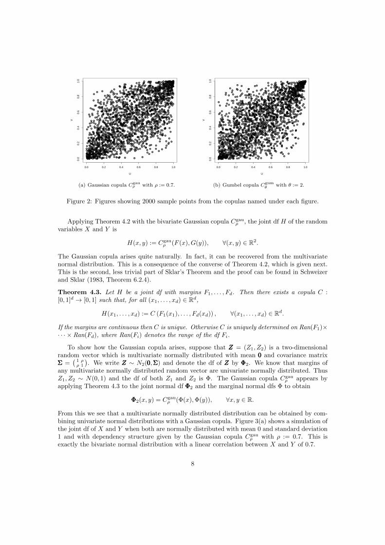
From this we see that a multivariate normally distributed distribution can be obtained by com-bining univariate normal distributions with a Gaussian copula. Figure 3(a) shows a simulation ofthe joint df of X and Y when both are normally distributed with mean 0 and standard deviation1 and with dependency structure given by the Gaussian copula Cgau
ρ with ρ := 0.7. This isexactly the bivariate normal distribution with a linear correlation between X and Y of 0.7.
8
Of course, we do not have to assume that the marginals are univariate normal distributions.For instance, Figure 2(a) shows a df which has standard uniform marginals with the Gaussiancopula Cgau
ρ with ρ := 0.7.
●
●
●●
●●
●
●●
●
●
●
●
●
●●
●
● ●
●
●
●
●
●
●●
●
●
● ●
●●
●
●
●
●
●
●●
●
●
●●
●●
●
●
●
●
●
●
●
●
●
●
●
●
●
●
●
●●
●
●
●
●
●
●
●
●
●
●
●
●
●●
●
●
●
●
●●
●
●
●●
●
●
●
●
●
●
●
●
●
●
●
●
●
●
●
●
●
●
●
●
●
●
●●
●
●
●●
● ●●
●
●
●
●
●
●
●
●
●
●
●
●
●
●
●
●
●
●
●
●
●
●
●
●
●
●
●
●
●
● ●
●
●
●
●
●
●
●
●
●
●
●
●
●
●
●
●
●
●
●
●
●●
●
●
●
●
●
●
●
●
●
●
●
●
●
●
●
●
●
●
●
●
●
●
●
●
●
●
●
●
●
●
●
●
●
●
●
●
●
●
●
●
●
●●
●
●
●
●
●
●
●
●
●
●
●
●
●
●
●
●
●●
●
●
●●
●
●
●
●
●
●
●
● ● ●
●
●
●●
●
●●
●
●
●
●
●
●
●
●● ●
● ●
●
●
●
●
●●
●
●
●
●
●
●
●
●
●
●
●
●
●
●
●
●
●●
●
●
●
●
●
●
●
●
●
●
●●
●
●
●
●
●
●
●
●
●
●
●
●●
●
●
●●
● ●
●
●
●
●
●
●
●
●
●
●
●
●
●
●
●●
●
●
●
●
●●
●
●
●
●
●
●
●
●●
●
●
●
●●
●
●
●
●
●●
●●●
●
●
●
●
●
●
●
●
●
●
●
●
●
●
●
●
●
●
●
●
●
●
●
●●
●
●
●
●
●
●
●
●
●
●
●
●
●
●
●
●
●
●
●
●
●
●●
●
●
●●
●●
●
●
●
●
●
●
●
●
●
●
●
●
●
●
●
●
●
●
●
●
●
●
●
●
● ●
●
●
●
●
●
●
●
●
●
●
●
●
●
●
●
●
●
●
●●
●
●
●
●
●
●
●
●
●
●
●
●
●
●
●
●
●
●
●
●
●
●
●
●
●
●
●
●
●
●
●
●
●
●
●
●
●
●
●
●
●
●
●
●
●
●
●
●
●
●
●
●
●
●
●● ●
●●
●
●
●
●
●
●
●
●
●
●
●
●
●●●
●●
●
●
●
●
●
●
●
●
●
●●
●
●
●
●
●
●●
●●
●
●●
●
●
●
●
●
●
●
●
●
●
●
●
●
●
●
●
●
●
●
●
●
●
●
●
●
●
●
●
●
●
●
●
● ●
●
●●
●
●●
●
●
●
●
●
●
●
●
●
●
●
●
●
●
●●
●
●
●
●
●
●
●
●
●
● ●
●
●
●
●
●
●
●
●
●
●
●
●
●
●
●
●
●
●
●
●
●
●
●
●
●
●
●
● ●●
●
●
●
●
●
●
●
●
●
●●
●
●
●
●
●
●
●
●
●●
●
●
●
●●
●
●●
●
●
●
●●
●
●
●
●
●
●
●
●
●
●
●
●●
●
●
●
●
●
●
●
●●
●●
●
●
●●
●
●
●
●
●
●
●
●
●
●
●
●
●
●
●
●
●
●
●
●
●
●
●●
●
●
●
●
●
●
●
●
●
●
●●
●
●
●●
●●
●
●
●●
●
●
●
●
● ●
●
●
●
●
●
●
●
●
●
●●
●
●
●
●
●
●
●
●
●
●
●
●
●
●
●●
●
●●
●
●
●
●
●
●
●
●
●
●
●
●
●
●
●
●
●
●
●
●
●
●
●
● ●
●
●
●
●
●
●
●
●
●
●
●
●
●
●
●
●
●
●
●
●
●
●
●
●
●
●
●
●
●
●
●
●
●
●
●
●
●
●
●
●
●
●
●
●
●
●
●
●
●
●
●
●
●
●
●●
●●
●●
● ●
●
●
●
●
●
●
●
●
●
●
●
●
●
●
●
●
●●
●
●
●
●
●
●
●
●●
● ●
●
●
●
●
●
●
●
●
●
●
●
●
●
●
●●
●
●
●
●
●
●
●
●
●
●
●
●
●●
●
●
●
●
●
●
●
●
●●●
●
●
●
●
●●
●
●●
●
●
●
●
●
●
●
●
●
●
●
●
●
●
●
●
●
●
●
●
●
●
●
●
●
●●●
●
●
●
●
●
● ●●
●
●
●
●
●
●
●
●●
●
●
●
●
●
●
●
●
●
●
●
●●
●
●
●
●
●
●
●
●●
●
●
●
●
●
●
●
●
●
●
●
●
● ●
●
●
●
●
●
●●
●
●
●
●●
● ●
●
● ●
●
●
●
●
●
●●
●
●
●●
●
●
●
●
●
●
●
●
●
●
●
●
●
●
●●
●
●
●
●
●
●
●
●
● ●
●
●
●
●
●
●
●
●●
●
●
●
●●
●●
●
●●
●●
●
●
●
●
●
●
●
●
●
●
●
●
●
●●
●
●●
●● ●
●
●
●
●
●
●
●
●
●
●
●
●
●
●
●● ●
●
●
●
●
●
●
●
●●
●
●
●
●
●
●
●
●
●
●
●
●
●
●●
●
●
●
●
●
●
●
●
●
●
●
●
●
●●
●
●
●●
●
● ●
●
●
●
●
●
●
●
●●
●
●
●
●
●
●
●
●
●
●●
●
●
●
●
●
●
●
●
●
●
●
●●
●
● ●
●
●
●● ●
●
●
●
●
●●
●
●
●●
●
●
●●
●
●
●
●
●
●
●
●●
●
●
●
●
●
●
●
●
●
●
●
●
●
●
●
●
●
●●●
●
●
●
●
●
●
●
●
●●
●
● ●
●
●
●
●
●
●
●
●
●●
●
●
●
●
●
●
●
●
●
●
●
●
●
●
●
●
●
●
●
●
●
●
●
●
●
●
●
●
●
●
●
●
●
●
●
●
●
●
●●
●
●
●
●●
●
●
●
●
●
●
●
●
●
●
●
●
●
●
●
●
●●
●●
●
●
●
●
●
●
●
●
●●
●
●
●
●
●
●
●
●
●●
●
●
●
●
●
●
●
●
●
●
●
●
●
●
●
●
●
●●
●
●
●●
●
●
●
●
●
●
●
●
●
●
●
●●
●
●
●
●
●
●
●
●
●
●
●
●●
●
●
●
●
●
●
●●
●
●
●
●
●
●
●
●
●
●
●
●●
●
●
●
●
●
●
●
●
●
●
●
●
●
●
●●
●
●
●
●
●
●
●
●
●
●
● ●
●
●
●
● ●
●
●
●
●
●
●●
●
●
●
●
●
●
●
●
●
●
●
●
●
●
●
●
●
●
●
●
●
●
●
●
●
●
●
●●
●
●
●●
●●
●●
●
●
●
●
●
●
●
●
●
●●
●
●
●
●
●
● ●
●
●
●
●
●●
●
●●
●
●
●
●
●
●
●
●
●
●
●
●
●
●●
●
●
●●
●●
●
●
●
●●
●
●●
●
●
●
●
●
●●
●
●
●
●
●●
●
●
●
●●●
●
●●
●
●
●
●
●●
●
●
●
●
●
●
●
●
●
●
●
●
●
●
●
●
●
●
●
●
●
●
●
●
●
●
●●
●
●
●
●
●
●
●
●
●
●
●
●
●
●
●
●
●
●
●
●
●
●
●
● ●
●
●
●
●
●
●
●
●
●
●
●
●
●
●
●
●
●
●
●
●
●
●
●
●
●●
●
●●
●
●
●
●
●
●
●
●
●
●
●
●
●
●
●
●
●
●
●●
●
●
●
●●
●
●
●
●
●
●
●●
●
●
●
●
●
●●
●
●
●
●
●
●
● ●
●
●
●
●
●
●
●
●
●
●
●
●
●
●
●●●
●
●
●
●
●
●
●
●
●
●●
●●
●
●
●
●●
●
●
●
●
●
●
●
●
●
●●
●
●
●●
●
●
●
●
●
●
●
●
●
●
●
●
●
●
●
●
●
●
●
●
●●
●
●
●
●●
●●
●
●
●
●
●
●
●
●●
●
●
●
●
●
●
●
●
●
●
● ●● ● ●
●
●
●
●
● ●
●
●
●
●
●
●
●
●
●
●
●
●
●
●
●●
●
●
●
●
●
●
●
●
●
●
●
●
●
●
●
●
●
●
●
●
●
●
●
●
●
●
● ●
●
● ●
●
●
●
●●
●
●
●
●●
●
●●
●
●
●
●
●
●
●
●
●
●
●
●
●
●
●
●
●
●●
●
●
●
●
●
●
●
●
●
●
●
●
●
●
●●
●
●
●
●
●●
●
●
●
●
●
●
● ●
●
●
●
●●
●
●
●
●
●
●
●●
●
●
●
●
●
●
●●
●
●●
●
●
●●
●
●
●
●
●
●
●
●
●
●
●
●
●
●
●
●
●
●
●
●
●
●
●
●●
●
●
●
●
●
●
●
●
●
●
●
●
●
●●
●
●
●
●
●
●
●
●●
●
●
●●
●
● ●
●
●
●
●
●
●
●
●
●
●
●
●
●
●
●
●
●●
●
●
●●
●
●
●
●
●●
●
●
●
●
●
●
●
●●
●
●
●
●
●●
●
●
●●
●
●
●
●
●●
●
●
●
●
●
●
●●
●
●
●
● ●
●
●
●
●
●
●
●
●
● ●
●
●●
●
●
●
●
●
●
●
●
●
●
●
●
●●
●
●
●
●
●
●
●
●
●
●
●
●
●
●
●
●
●
●
●
●
●
●
●
●●
●
●
●●
●
●
●
●
●
●
●
●
●
●
●
●
●
●
●
●●
●
●
●
●
●
●
●
●
●
●
●
●
●
●
●
●
●
●
●
●
●
●
●●
●●
●
●
●●
●
●
●
●
●
●
●
●
●
●
●
●
●
●
●
●
●
●
●
●●
●●
●
●
●
●
●
●
●
●
●
●
●
●
●
●
●
●
●
●
●
●
●
●
●
●
●
●
●
●
●
●
●●●●
●
●
●
● ●
●
●
●
●
●
●●
●
●●
●
●
●
●
●
●
●
●
●
●
●
●●
●●
●
●
●
●
●
●
●
●
●
●
●
●
●
●
●
●
●
●
●
●
●
●
●
●
●
●
●●
●
●
●
●
●
●
●
●
●
●
●
●
●
●
●
●
●
●
●
●
●
●
●
●
●
●●
●
●
●
●
●
●
●
●
●
●
●
●
●
●
●
●
●
●
●
●
●
●
●
●
●
●
●
●
●
●
●
●
●
●
●
●
●
●
●●
●
●
●
●
●●
●
●
●
●
●
●
●
●
●
●
●
● ●
●
●
●
●
●
●
●
●
●
●
●
●●
●
●
●
●
●
● ●
●
●
●
●
●
●
●
●
●
●
●●
●
●
●
●
●
●●
●
●
●
●
●
●
●
●
●
●
●
●
●
● ●●
●
●
●
●
●
●
●
●
●
●
●
●
●
●
●
●
●
●
●●
●
●
●
● ●
●
●●
●●
●
●
●
●
●
●
●
●
●
●
● ●
●
●
●
●
●
●
●
●
●
●
●
●
●
●
●
●
●
●
●
●
●
●
●●
●
●
●
●
●
●
●
●
●
●●
● ●
●
●
●
●
●
●
●
●
●
●
●●
●
●
●
●●
●
●
●
●
●●
●
●
●
●
●
●●●
●
●
●
●
●
●
●
●
●
●
●
●
●
●
●
●
●
●
●
●
●
●●
●
●
●
●
●
●
●
●●●
●
●
●
●
●
●
●
●
●
●
●
●
●
●
●
●
●
●
●
●
●
●
●
●
●
●
●
●
●
●
●
●●
●
●
●
●
●
●
●
●
●
●
●
●
●
●
●
● ●
●
●
●
●
●
● ●
●
●
●
●
●
●
●
●
●
●
●
●
●
●
●●
●
●
●●
●
●●
●
●
●
●
●
●
●
●●
●
●
●
●
●
●
●
●
●
●
●
●
●
●
●
●
●
●
●
●
●
●
●
●
●
●
●
●
● ●
●●●
●
●
●
●
●
●
●
●
●
●
●
●
●
●
●
●
●
●●
●
●
●
●
●
●
●
●●
●
●
●
●●
●
●
●
●
●●
●
●
●●
●
●●
●
●
●●
●
●●
●
●
●●
●
●
●
●
●
●
●
●
●
●
●
●
●
●
●
●
●
●●●
●
●
● ●
●
●
●
●
●
●
●
●
●
●
●
●●
●
●●●
●
●
●
●
●
●
●●
●
●
●
●
●
●●
●
●
●
●
●
●
●
●
●
●
●●
●
●
●
● ●
●
●●
●
●
●
●
●
●●
●●
●●
●
●
●●
●
●
●●
● ●●
●
●
●
●●
●
●
●
●
●
●
●
●
●
●
●
●
●
● ●
●
●
●
●
●
●
●
●
●
●
●
●●
●
●
●
●
●
● ●●
●●
●
●●
●
●
●
●
●
●
●
●●
●
●●
●
●
●
●
●●
●
●
●
●
●
●
●
●
●
●
●●●
●
●
●
●
●
●
●
●
●
●
●
●
●●
●
● ●
●
●
●
●
●●
●
●
●
●
●
●
●●
●●
●
●
●
●
●
●
●●
●
●
●
●
●
●
●
●
●
●
●
●
●
●
●
●
●
●●
●
●
●
●
●
●
●
●
●●●
●
●
●
●
●
●
●
●
●
●
●
●
●
●●
●
●●
●
●
●
●
●
●●
●
●
●
●●
●
●
●
●
●
●
●
●
●
●
●
●
●
●
●
●
●
●
●
●●●
●
●
●●●
●
●●
●
● ●
●
●
●●
●
●
●
●
●●
●
●
●
●
●
●
●
●
●
●●
●
●●
●
●
●
●●
●
●●
●
●
●
●
●
●
●
●
●
●
●
●
●
●
●
●
●
●
●
●
●
●
●
●
●
●
●
●
●
●
●
●
●
●
●
●
●
●
●●
●
●
●
●●
●
●
●●
●
●
●
●
●
●●
●
●
● ●
●
●
●
●●
●
●● ●
●
●
●
●
●
●
●
●
●
●
●
●
●●
●
●
● ●
●●
●
●
●
●
●
●
●
●
●●
●
●
●
●
●
●
●
●
●
●
●
●
●
●
●
●●
●
●
●
●
●
●
●
●
●
●
●
●
●
●●
●
●
●
●
●
●
●
●
●
●
●●
●
●
●
●
●
●
●
●
●
●
●
● ●
●
●
●
●
●●
●●
●
●
●
●
●
●
●
●
●● ●
●
●
●
●
●
●
●
●●
●
●
●
●
●
●
●
●
●●
●
●
●
●
●
●
●
●
●
●
●
●
●
●●●
●
●
●
●
●
●
●●
●
●●
●
●
●
●
●
●
●
●
●
●
●
●
●
●●
● ●
●
●
●
●
●
●
●
●
●
●
●
●
●
●
●
●
●
●●
●
●
●●
●
●
●
●●
●
●
●
●
●
●
●
●
●
●
●●
●
●
●
●
●
●
●
●
●
●
●
●
●●
●
●
●
●
●
●
●
●
●
●
●
●
●
●
●
●
●
●
●
●
●●
●
●●
●
●
●
●
●
●
●
●
●
●
●
●
●
●
●
●
●
●
●
●●
●
●
●
●
●
●
●
●
●
●
●
●
●
●
●●
●
●
●
●
●
●
●
●
●
●
●
●
●
●
●
●
●
●
●
●
●
●●●
●
●
●
●
●
●
● ●● ●
●
●
●●
●
●
●
●
●
●●
●
●●
●
●●
●
●
●
●
●●
●
●
●
●
●
●
●●
●
●
●
●
●●
●
●
●
●
●
●
●
●
●
●
●
●
●
●
●
●●
●
●
●●
●
●●
●
●
●
●
●
●
●●
●
●
●
●
●
●
●
●
●
●●
●
●●●
●
● ●
●
●
●
●
●●● ●
●
●●
●
●
●
●
●
●
●
●
●
● ●
●●
●
●●
●
●
●
●
●●
●●
●●
●
●●
●
●
●
●
●
●
●
●
●
●
●
●●
●
●
●
●
●
●
●
●
●
●
●
●
●
●
●
● ●
●●
●
●
●
●
●
●
●
●
●
●
●
●
●
●
●
●
●
●
●
●
●
●●
●
●
●
●
● ●
●
●
●
●
●
●
●
●
●
●
●
●
●
●
●
●
●
●
●
●
●
●
●
●
●
●
●
●
●
●
●
●
●
●
● ●
●
●
●
●●●
●
●
●
●
●
●
●
●
●●
●
●
●
●
●
●
●●
●
●
●
●●
●
●
●
●
●●
●
●●
●
●
●●
●●
●
●
●
●
●
●
●
●●
●
●●
●
●
●
●
●
●
●
●
●
●
●
●
●
●
●
●
●
●
●
●
●
●
●
●
●
●
●
●
●
●
●
● ●
●
●
●
●
●
●
●
●
●
●
●
● ●
●● ●
●
●
●●
●
●
●
●
●
●
●
●
●
●
●
●
●●
●●●
●
●
●
●●
●●
●
●
●
●
●
●
● ●
●
●
●
●
●
●●●
●
●
●
●
●
●
●
●
●●●
●
●
●
●
●
●
●
●
●
●
●
●
●●
●
●●●
●
●●
●
●
● ●●
●
●
●
●
●
●
●
●
●
●●
●
●
●
●
●
●
●
●
●
● ●
●
●
●
●
●
●
●
●
●●
●●
●
●
●
●
●
●
●
●
●
● ●
●
●
●●
●
●
●
●
●
●
●
●
●
●
●
●
●●
●
●●
●
●
●
●
●
●
●
●
●●
●
●
●
●
●
●
●
●
●
●
●
●
●
●
●
●
●●
●
●
●
●
●
●
●
●
●
●
●
●
●
●
●
●
●
●
●
●
● ●
●
●
●●
●●
●●
●
●
●
●
●
●
●
●
●
●
●●
●
●
●
●
●
●
●●
●
●●●
●
●
●
●
●
●
●●
●
●
●
●
●
●
●
●
●
●
●
●
●
●
●
●
●
●
● ●
●●
●
●
●
●
●●
●●
●●●
●
●
●
●
●
●
●
●●
●
●
●
●
●
●
●
●
●
●
●●
●
●
●
●
●
●
●
● ●
● ●●
●
●●
●
●
●
●
●
●
●
●
●
●
●
●
●
●
●
●
●
●
●
●
●
●
●
●
●
●
●
●
●
●
●
●
●
●
●
●
●
●
●
●
●
●●●
●
●●
●
●
●
●
●
●●
●
●
● ●
●
●
●
●
●
●
●
●
●
●
●
● ●●
●
●
●
●
●●
●
●
●
●●
●
●
●
●
●
●
●
●
●
●●
●
●
●
●
●
●
●
●●
●
●
●
●
●
●●
●
●
●
●
●
●
●
●
●●
●
●● ●●
●
●●
●
●●
●
●
●
●
●
●
●
●
●
●
●
●
●
●
●
●
●
●
●
●●
● ●
●
●●
●
●
●●
●
●
●●
●
●
●
●
●
●
●
●
●
●
●
● ●
●
●
●
●
●
●
●
●
●●
●
●●
●
●
●
●
●
●
●
●
●
●
●
●
●
●
●
●
●
●
●
●
●
●
●
●
●
●
●
●
●
●
●
●
●
●
●
●
●
●
●
●
●
●
●
●
●
●
●
●
● ●
●
●
●
●
●
●
● ●
●
●
●
●
●
●
●
●
●
●●
●
●
●●
●●
●
●
●●
●
●
●
●
●●
●
●
●●
●
●
●
●
●
●
●
●
●
●
●
●●
●
●
●
●
●
●
●●
●
●
●
●
●
●
●
●●
●
●
●
●
●
●
●
●
●
●
●●
●
●
●
●●
●
●
●
●
●
●
●
●●●
●
●
●
●
●
●
●
●
●
●●
●
●
●
●
●
●
●
●
●
●
●
●
●
●
●●
●
●
●●●
●
●
●
●
●
●●
●
●●
●
●
●
●
●
●●
●●
●
●
●
●
●
● ●●
●
●
●
●
●
●
●
●
●
●
●
●
●
●
●
●
●
●
●
●
●
●●
●
●
●
●
●
●
●
●
●
●
●
●
●
●
●
●
●
● ●
●
●
●
●
●
●
●
●
●
●
●
●
●
●●●
●
●
● ●
●
●
●
●●
●
●
●
●●
●●●
●
●●
●●
●
●●
●
●
●
●
●
●
●
●
● ●
●
●
●
●
●
●
●
●
●
●
●
●
●
●
●
● ●●
●
●
●
●
●
●
●
●
●
●
●
●
●
●
●
●
●
●
●
●
●
●
●
●
●●
●
●
● ●
●
●
● ●
●●
●
●
●
●
●
●
●●
●
●
●
●
●
●
●
●
●
●
●
●●
●
●
●
● ●
●
●
●
●
●
●
●●
●
●
●
●
●
●
●
●
●
●
●
●
●
●
●
●●
●
●
●
●
●
●
●
●●
●
●
●
●●
●
●
●
●
●
●
●
●
●
●
●
●
●
●●
●
●
●
●
●
●
●
●
●
●
●
●
●
●
●
●
●
●
●●
●
●
●
●
●
●
●
●
●
●
●
●
●
●
●
●
●
●
●
●
●
●
●●
●
●
●
●
●
●
●●
●
●
●
●
●
●
●
●
●
●
●
●
●
●
●
●
●
●
● ●
●
●
●
●
●
●●
●●
●●
●
●
●
●
●
●
●
●
●
●
●
●
●
●
●
● ●
●●
●
●
●
●
●
●
●
●
●
●
●
●
●
●
●
●
●
●
●
●
●
●
●
●
●
●
●
●
●
●
●
●●
●
●
●
●
●
●● ●
●
●
●
●
●
●●
●
●
● ●●●
●●●
●
●●
●
●
●
●
●
●
●
●
●●
●
●
●
●
●
●●
●
●
●
●
●
●
●
●
●
●
●
●
●
●
●
●
●
●
●
●
●
●
−4 −2 0 2 4
−4
−2
02
4
X
Y
(a) Gaussian copula Cgauρ with ρ := 0.7.
●
●
●
●
●
●
●
●●
●
●
●●
●
●
●
●
●
●
●
●
●
●
●
●
●
●
●
●●
●
●
●
●
●
●●●
●
●●
●
●
●
●
●
●
●●
●●
●
●
●
●
●
●
●
●
●
●
●
●
●
●
●
●
●
●
●
●
●
● ●
●
●
●
●
●●
●●
● ●
●●
●
●
●
●
●
●
●
●
●
●
●
●
●
●
●
●
●
●
●
●
●
●
●●
●
●●
●
●
●
●●
●
●
●
●●
●
●
●
●
●
●
●
●
●
●●
●
●
●
●●
●
●
●
●●
●
●
●
●
●
●
●
●
●
●
●
●
●
●
●
●
●
●
●
●
●
●
●
●
●
●
●
●
●
●
●●
●
●
●
●
●
●
●
●
●
●
●
●
●
●
●
●
●
●
●
●
●
●
●
●
●
●
●
●
●
●
●
●●
●
●
●
●
●
●
●●
●
●
●
●
●
●
●
●
●
●
●
●●
●
●
●
●●
●
●
●
●
●●
●
●
●
●●
●
●
●
●
●
●
●
●
●
●
●
●
●
●
●
● ●
●
●
●
●
●
●
●
●
●
●
●
●
●
●
●
●
●
●●
●
●
●
● ● ●
●
● ●
●
●
●
●
●●
●
●●
●
●
●
●
●
●
●
●
●
●
●
●
●
●
●
●
●
●
●
●
●
●
●
●
●●●
●
●
●●
●
●
●
●
●
●
●
● ●
●
●
●
●
●
●
●
●●
●
●
●
●
●
●
●
●
●
●
● ●
●●
●
●
●
●●
●
● ●
●
●
●
●
●
●
●●
●
●
●
●●
●
●
●●
●●
●
●
●
●
●
●
●
●
● ●
●
●
●
●
●
●●
●●
●
●
●
●
●
●
●
●
●
●
●●
●
●
●
●
●●
●
●
●
●●
●
●
●
●
●
●
●
●
●
●
●●
●●
●
●
●●
●
●
●●
●●
●
●
●
●
●
●
●
●
●
●
●
●
●
●
●
●
●
●
●
●
●
●
●
●●
●
●
●
●
●
●
●
●
●
●
●
●
●
●
●●
●
●
●
●
●
●
●
●
●
●
●●
●
●
●●
●
●
●
●●
●
●
●
●
●
●
●
●
●
●
●
●
●●
●
●
●
●
●
●●
●
●
●●
●
●
●
●
●
●●
●
●●
●
●
●
●
●
●
●
●
●
●
●
●
●
●
●
●
●●
●
●
●
●
●
●
●
●●
●
●
●
●
●
●
●
●
●
●
●
●
●
●
●
●
●
●
●
●●
●
●
●
●
●
●
●
●
●
●●
●
●
●
●
●
●
●
●
●
●
●
●●
●
●
●
●●
●●●
●
●
●
●
●●●
●
●
●
●
●
●●
●
●
●
●
●
●
●
●
●
●
●
●
●
●
●
●●
●
●●
●
●
●
●
●●
●
●
●
●
●
●
●
●
●
●
●
●
●
●
●
●
●
●
●
●
●●
●
●
●
●
●
●● ●
●
●
●
●
●
● ●
●
●
●
●
●
●
●
●
●
●
●
●
●
●
●
●
●
●
●
●
●●
● ●
●
●
●
●
●
●
●
●
●
●
●
●
●
●
●
●●
●
●
● ●●
●
●
●
●
●
●
●
●
●●
●
●
●
●
●
●
●
●
●
●
●●
● ●
●
●
●
●●
●
●
●
●
●
●
●
●
●
●
●
●●
●●
●
●●
●
●
●
●
●
●
●
●
●
●
●
●
●
●●
●
●●
●
●
●
●
●
●
●
●
●
●
●
●
●
●
●
●
●
●
●
●
●
●
●
●
●
●
●
●●
●
●
●
●●
●
●
● ●
●
●● ●
●
●
●
●
●
●
●
●
●
●
●
●
●
●
●
●
●
●
●●
●
●
●
●● ●
●
●
●
●
●
●
●
●●
●
●
●
●
●
●
● ●
●
●
●
●
●
●
●
●
●●
●
●
●
●●
●
●
●
●
●
●●
●
●
● ●
●●
●
●
●
●
●
●
●
●
●
●
●●
●
●
●
●
●
●
●
●●
●
●
●
●
●
●
●
●
●
●
●●
●
●
●
●
●
●
●
●
●
●
●●
●
●
●
●
● ●
●
●
●
●●
●
●
●
●
●
●
●
●
●
●
●
●
●
● ●
●
●●
●
●
●
●
●
●
●
●
●
●
●●
●
●
●●
●
●
●●
●
●
●
●
●
●
●●
●
●
●
●
●
●
●
●
●
●
●
●
●
●
●
●
●
●
●
●
●
●●
●
●●
●
●
●
●
●
●
●
●
●
●
●●
● ●
●
●
●
●
●●
●
●
●
●
●
●
●
●
●●
●
●
●
●
● ●
●
●
●
●
●
●
●
●
●
●
●
●
●
●
●
●
●
●
●
●
●
●
●
●
●
●
●
●●
●
●
●●
●
●
●
●
●
●
●
●
●
●
●
●
●
●
●
●
●
●
●
●●
●
●
●
●●
●
●
●
●●
●
●
●
●
●
●
●
●
●●
●●
●
●
●
●
●
●
●
●
●
●
●
●
●
●
●
●
●
●●
●
●
●
●
●
●
●
●
●
●
●
●
●
●
●
●●
● ●
●
●
●
●●
●
●
●
●
●
●
●
●
●
●
●
●
●
●
●
●●
●
●
●
●
●
●
●
●
●
●
●
●
●
●
●
●
●
●●
●
●
●
●
●
●
●
●
●
●
●
●
●
●
●
●
●
●
●
●
●
●
●●
●
●
●
●
●●
●
●
●
● ●
●●
●
●
●
●
●●
●
●
●
●
●
●
●
●
●
●
●
●●
●●
●
●
●
●
●
●
●
●
●
●
●
●
●●
●
●
●
●●
●
●
●
●
● ●
●
●
●
●
●
●
●
●
●
●
●
●
●
●
●
●
● ●
●
●
●
●
●
●
●
●
●
●
●
●
●
●
●
●
●
●
●
●
●
●
●
●
●
●●
●
●
●
●
●
●
●
●
●
●
●
●
●
●
●
●
●
●
●
●
●
●
●
●
●
●
●
●
●
●
●
●
●
●
●
●●
●●
●
●
●
●
●
●
●
●●
●
●
●
●
●
●
●
●
●
●
●
●
●
●
●
●
● ●●
●
●
●
●
●
●●
●
●
●
●
●●
●
●
●
● ●
●
●
●
●
●
●
●
●
●
●
●
●
●
●
●
●
●
●
●
●
●
●
●
●
●
●
●
●
●
●
●
●
●● ●
●
●
●
●
●●
●
●
●
●
●●
●
●●
●
●
●
●
●
●
●
●
● ●
●
●●
●
●
●●
●
●
●
●
●
●
●
●●
●
●
●
●
●
●
●
●
●●
●
●
●
●
●
●
●
●
●
●
●
●
●
●
●
●
●
●
●
●
●
●
●
●
●
●
●
●
●
●
●
●
●
●
●
●
●
●
●
●
●
●
●
●●
●
●
●
●
●
●
●
●
●●
●
●
●
●
●
●
● ●
●
●
●
●
●
●
●
●
●
●
●
●
●●
●
●
●
●
●
● ●
●
●
●
●
●
●●
●
●
●
● ●
●
●
●
●
●
●
●
●
●
●
●
●
●●
●
●
●
●
●
●
● ●
●
●
●
●
●
●
●
●
●
●
●
●●
●
●
●
●
●
●
●●
●
●●●
●
●
●
●
●
●
●
●
●●
● ●
●
●
●
●●
●
●
●●
●
●
●
●
●
●
●●
●
●
●
●
●●
●
●
●
●
●
●
●
●
●
●
●
●
●
●
●
●
●
●
●
●
●
●
●
●
●
●
●
●
●●
●
●
●
●
●
●
●
●
●
●
●
●
●
●
●
● ●
●
●
●
●●
●
●
●
●
●
●
●
●●
●●
●
●
●
●
●
●●
●
●
●
●
●
●
●
●
●
●
●
●
●
●
●●
●
●
●
●
●
●
●●
●
●
●
●
●
●
●
●
●
●
●
●
●
●
●
●●
●
●
●
●
●
●
●
●
●●
●
●
●
●
●●
●
●
●
●
●
●
●
●
●
●
●
●
●
●
●●
●
●
●
●
●
●
●
●
● ●
●
●
●
●
●
●
●
●
●
●●
●
●
●
●
●
●●●
●
●
●●
●
●
●
● ●
●
●
●
●
●
●
●
●
●
●
●
●
●
●
●
●
●
●
●
●
●
●
●
●
●
●
●
●
●
● ●
●
●
●
●
●
●
●
●
●
●
●
●
●
●
●
●
●
●
●
●
●●
●
●
●
●
●
●
●
●
●
●
●●
●
●
●
●
●
●
●
●
●
●
●
●
●●
●
●
●
●
●
●
●
●
●
●
● ●
●
●
●
●
●
●●
●
●
●●
●
●●●
●
●
●
●●
●
●
●
●
●
●
●
●
●
●
●
●
●
●
●
●
●●
●
●
●
●
●
●
●●
●
●
●
●
●
●
●
●
●
●
●
●
●
●
●
●
●
●
●
●●
●
●
●
●
●
●
●
●
●
●
●
●
●
●
●
●
●
●
●
●
●
●
●
●
●
●
●
●●
●
●
●
●
●
●
●
●
●●
●
●
●
●
●
●
●
●
●
●
●
●
●
●
●
●●
●
● ●
● ●
●
●
●
●
●●
●
●
●
●
●
●
●
●
●
●
●
●
●
●
●
●
●●
●
●
●
●●
●
●
●
●
●
●
●
●
●
●
●
●
●
●
●●
●
●
●
●
●
●
●
●
●
●●
●
●
●
●
●
●
●
●
●
●
●●
●
●
●●
●
●
●
●
●
●●●
●
●
●
●
●
●
●
●
●
●
●
●
●
●
●
●
●
●
●
●
●●
●
●
●
●
●
●
●
●
●
●
●
●
●
●
●●
●
●
●
●
●
●
●
●
●
●
●
●
●
●
●●
●
●● ●●
●
●●
●
●
●
●
●
●
● ●●
●
●
● ●
●
●
●
●
●
●
●
●
●
●
●
●
●
●
●
●
●
●
●
●
●
●
●
●
●
●
●
●●
●
●
●
●
●
●
●
●
●
●
●
●
●
●
●
●
●
●
●
●●
●
●
●
●
●
●
●● ●●
●
●
●
●
●
●
●
●
●
●
●
●
●●
●
●
●
●
●
●
●
●
●
●
●
●
●
●
●●
●
●
●
●
●
●
●
●
●●
●
●
●
●
●
●
●
●
●
●
●
●●
●
●
●
●
●
●
●
●●
●
●
●
●
●
●
●●
●
●
●
●
●
●
●
●
●
●
●
●●
●
●
●
●
●
●
●●
●
●
●
● ●
●
●●
●●●
●
●
●
●
●
●
●
●
●
●
●
●
●
●
●●
●
●
●
●
●
●
●
●
●
●●
●
●
●
●
●
●
●
●
●
●
●
●
●
●
●
●●
●
●
●
●
●
●●
●
●
●
●
●
●●
●
●
●
●
●
●●
●
●
●
●
●●●
●
●
●
●
●
●
●
●
●
●
●
●●
●
●
●●
●●
●
●
●
●
●
●
●
●
● ●
●
●
●
●
●
●
●
●●
●
●
●
●
●
●
●
● ●
●●
●
●
●
●●
●
●
●●
●
●
●
●
●
●
●
●
●
●
●●
●
●
●
●
●
●
●
●●
●●
●
●
●
●
●
●●
●
●
●
●
●
●
●
●
●
●
●
●
●
●
●
●
●
●
●
●
●
●
●
●
●
●
●
●
●
●
●
●
●
●
●●
●
●
●
●
●
●
●
●
●
●
●
●
●
●
●
● ●
●
●
●
● ●
●
●
●
●
●●
●
●
●
●
●
●
●
●
●
●
●
●
●
●
●
●
●●
●
●
●
●
●
● ●
●
●
●
●
●
●●
●
●
●
●
●
●
●
●
●●
●
●
●● ●
●
●
●
●
●●
●
●
●
●
●
●
●
●●
●
●
●
●
●
●
●
●
●
●
●●
●
●
●
●
●
●
●
●●
●
●
●
●
●
●
●
●
●
●
●
●
●
●
●●
●
●
●
●
●
●
●
●
●
●
●
●
●
●
●
●
●
●●
●
●
●
●
●
●
●●
●
●
●
●
●
●
●
●
●
●
●
●
●
●
●●
●
●
●
●
●
●
●●
●
●
●
●
●
●
●●●
●
●
●
●
●
●
●
●
●
●
●
●
●●
●
●
●
●
●
●
●
●
●
●●
●
●
●
●
●
●
●
●
●
●
●●
●
●
●
●
●
●
●
●
●
●
●
●
●●
●
●
●
●
●
●
●
●
●
●
●
●
●
●
●
●
●
●
●
●
●●
●
●●
●●
●●
●
●
●
●
●
●
●
●●●
●
● ●
●
●●
●
●
●●
●
●
●
●
●
●
●
●
●
●
●
●
●
●
●
●
●●
●
●
●
●
●
●
●
●
●
●●
●
●
●
●
●
●●
●
● ●●
●
●
●
●
●
●
●●
●
●
●
●
●
●●
●
●
●
●
●
●
●
●
●●
●
●
●
●
●
●
●
●
●
●●
●
●
●
●
●
●
●
●
●
●
●
●
●
●
●●
●●
●
●
●
●
●
●●
●
●
●
●
●
● ●
●●
●
●
●
●
●
●
●
●
●●
●
●●
● ●
●
●
●
●
●
●
●
●
●●
●
●
●
●
●
●
●
●
●●
●
●
●
●
●●
●
●
●
●
●
●
●
●
●
●●
●
● ●
●
●
●●
●
●
●
●
●
●
●
●
●●
●
●
●
●
●
●
●
●
●
●
●
●
●
●
●
●
●
●
●
●
●
●
●
●
●
●
●
●
●
●●
●
●●
●
●
● ●●
●
●
●●
●
●
●
●
●●
●
●
●
●
●
●●
●
●
● ● ●
●
●
●
●
●
●
●
●●
●
●
●
●
●●
●
●
●
●
●●
●
● ●
●
●
●
●
●●
●
●
●
●
●
●
●
●
●
●
●
●
●
●●
●
●
●
●
●
●
●
●
●●
●
●
●
●
●
●
●
●
●
●
●
●
●
●
●
●
●
●●
●
●
●●
●
●
●
●
●
●
●
●●
●
●
●
●
●
●
●
●
●
●
●
●
●
●
●
●
●
●
●
●
●
●
●
●
●
●
●
●
●
●
●
●
●
●●
●
●
●
●
●
●
● ●
● ●●
●
●
●
●
●●
●
●
●
●
●
●
●
●
●
●
●
● ●
●
●
●
●
●
●
●
● ●
●
●
●●
●
●
●
●
●
●
●●
●
●
●
●●
●
●
●
●
●
●
●
●
●
●
●
●
●●
●
●
●●
●
●
●
●
●
●
●
●
●
●
●
●
●
●●
●●
●
●
●
●
●
●
●
●
●
●
●
●
●
●
●
●
●
●●
●
●●
●
●
●
●
●
●
●
●
●
●
●
●
●
●
●
●
●
●
●
●● ●
●
●
●
● ●
●
●
●
●●
●
●
●
●
●
●●
●
●
●
●
●
●
●
●
●
● ●
●
●
●
●
●●
●
●
●
●
●
●
●
●
●
●●
●●
●
●
●
●
●
●
●
●
●
●
●
●
●
●
●●
●
●
●
●●
●
●
●
●
●
●
●
●
●●
●
●
●
●
●
●
●
●
●
●
●
●
●
●
●
●
●
●
●
●
● ●
●
●●
●
●
●
●
●
●
●
●
●
●
●
●
●●
●
●
●
●
●
●
●
●
●
●
●
●
●
●
●
●
●
●
●●
●
●●
●
●
●
●
●
●
●
●●
●
●●
●
●●
●
●
●
●
●
●
●
●
●
●
●●
●
●
●●
●
●
●
●
●
●
●
●
●●
●
●
●
●
●
●
●
●
●
●
●
●
●
●
●●
●●
●
●
●
●
●
●
●
●
●
●
●●
●
●
●
●
●
●
●●
●
●
●
●
●
● ●
●●
●
●
●
●
●
●
●
●
●
●●
●
●●
●
●
●
●●●
●
●
●
●
●●
●
●
●
●
●
●
●
●
●
●
●
●
●
●
●
●
●●
●
●
●
●
●
●
●
●
●●
●●
●
●
●
●
●
●
●●
●
●
●
●
●
●
●
●●
● ●
●
●
●
●
●
●
●
●
●
●●
●●
●
●
●
●
●
●
●
●
●
●
●●
●●
●
●
●
●
●
●
●
●
●
●
●
●
●
●●
●
●
●
●●
●
●
●
●
●
●
●
●
●
●
●
●
●
●
●
●
●
●
●
●
●●
●
●
●●
●
●
●
●
●
●
●
●
●
●●
●
●●
●
●
●
●
●
● ●
●
●
●
●
●
●
●
●
●
●
●
●
●
●
●
●
●
●
●
●
●
●
●
●
●
●
●
●
●
●
●
●
●
●
●
●
●
●
●
●
●
●
●●
●
●
●
●
●
●
●
●
●
●
●
●
●
●●
●
●
●
●
●
●
●
●
●
●
●●
●
●
●●
●
●
●
●
●
●
●
●
●
●
●
●
●
●
●
●
●
●
●
●
●
●
●
●
●
●
●
●
●
●
●
●
●
●
●
●
● ●
●
●
●
●
●
●
●
●
●
●
●
●●
●●
●
●
●●
●
●
●
●
●
●
●
●
●
●
●
●
●
● ●
●
●●
●
●
●
●●●
●
●
●
●
●●
●
●
●
●
●
●
●
●
●
●
●●
●
●
●
●
●
●
●
●
●
●
●
●
● ●
●
●
●●
●
●
●
●
●
●●
●
●
●
●
●●
●
●
●
●
●
●●●
●
●
●
●
●
●
●
●
●
●●
●
●
●
●
●
●
●
●
● ●
●
●
●
●
●
●
●
●
●
●
●
●
●
●
●
●
●
●
●
●
● ●
●
●●
●●
●
●
●
●●
●
●
●
●
●
●
●
●
●●
●
●
●
●
●
●
●
●● ●
●
●
●
●
●
●
●
●
●●
●
●
●
●
●
●
●
●
●
●
●
●
●
●
●
●●
●
●
●
●
●●
●
●●
●
●
●
●●
●
●
●
●
●
●
●
●
●
●
●
●
●
●
●
●
●
●
●
●
●
●
●●
●
●
●
●
●
●
●
●
●
●
●
●
●
●
●
●
●●
●
●
●●
●
●
●
●
●
● ●
●
●
●
●
●
●
●
●
●
●
●
●
●
●
●
●
●
●
●
●
●
●
●
●
●
●
●
●
● ●
●
●
●
●
●
●
●
●
●
●
●
●
●
●
●
●
●
●
●●
● ●
●
●●
●
●
●
●●
●
●
●
● ●●
●
●
●
● ●
●●
●
●
●
●
●
●
●
●
●
●
●
●
●
●
●
●
●
●
●
●
●
●
●
●
●
●
●
●
●
●●
●
●
●
● ●
●
●
●
●
●
●●
●
●
●
●
●
●
●
●
●
●
●
●
●
●
●
●
●
●
●
●
●
●
●
●
●
●
●
●
●
●
●
●
●
●
●
●
●
●●
●
●
●
●●
●
●
●
●
●
●
●
●
●
●
●●
●
●
●
●
●
● ●
●
●
●
●
●
●
●
●
●
●
●
●
●
●
●
●●
●
●
●
●
●
●
●
●
●
●
●
●
●
● ●
●
●
●
●
●
●
●
●
●
●
●
●
●
●
●
●
●
●
●
●
●
●
●
●
●
●●
●
● ●●
●
●
●
●
●
●
●
●
●●
●●
●
●
● ●
●
●
●
●
●
●
●
●
●
●
●●
●
●
●
●
●●
●●
●
●
●●
●
●
●
●
●
●
●
●
●
●
●●
●
●
●●
●
●
●
●
●
●
●
●
●
●
●
●
●
●
●
●
●
● ●●
●
●
●
●
●
●
●
●
●
●
●
●●
●
●
●
●
● ●
●
●
●
●●
●
●
● ●
●
●●
●
●
●
●
●
●
●
●●
●●
●
●●
●
●
●
●
●
●
●
●
●
●
●
●
●
●
●
●
●
●
●
●
●
●
● ●
●●
●
●
●
●
●
●
●
●
●
●
●●
●●
●
●
●
●●●
● ●●
●
●
●
●
● ●
●●
●
●
●
●
●
●
●
●
●
●
●
●
●
●
●
●
●
●
●
●
●
●
●
●
●●
●
● ●
●
●
●
●
●●
●
●
●
●
●
●
●
●
●
●●
●
●
●
●
●
●●
●
●
●
●
●
●
●
●
●
●
●
●
●
●
●
●
●
●
●
●
●
●
●
●
●
●
●
●
●
●
●
●
●
●
●●
●
●
●
●
●
●
●
●
●
●
●
●
●
●
●
●
●●
●
●●
●
●
●
●
●●
●
●
●
●
●
●
●
●
●
●
●
●
●
●
●
●
●
●
●
●
●
●●
●
●
●
●
●
●
●
●
●
●
●
●
●●
●
●
●●
●
●
●
●
●
●
●
●
●
●●
●
●
●
●
●
●
●
●
●
●
●
●
●
●
● ●● ●
●●
●
●
●
●
●
●
●
●●
●
●
●
●
●
●
●
●
●
●●
●
●
●
●
●
● ●
●
●
●
●
●●
●
●
●
●
●
●
●
●
●
●
●
●
●
●
●
●●
●●
●
●
●
●
●
●
●
●
●
●
●
●
●
●
●●
●
●
●
●
●
●
●
●
●
●
●
●
●
●
●
●
●
●
●
●
●
●
●
●
●
●
●● ●
●
●
●●
●
●
●
●
●●
●
●
●
●
●●
●●
●
●
●
●
●
●
●
●
●
●
●
●
●
●
●
●
●
●
●
●
●
●
●
●
●●
●●
●
●
●
●
●
●
●
●
●
●
●●●
●
●
●
●
●
●
●
●
●
●
●
●
●
●●
●
●
●●
●
●
●●
●
● ●
●
●
●
●
●
●
−4 −2 0 2 4
−4
−2
02
4
XY
(b) Gumbel copula Cgumθ with θ := 2.
Figure 3: Figures showing 5000 sample points from the random vector (X,Y ) which has standardnormally distributed margins and dependency structure as given by the copula named under eachfigure. To the right of the vertical line x = 2 and above the horizontal line y = 2, in the Gaussiancopula figure there are 43 sample points. The corresponding number for the Gumbel copula figureis 70. To the right of the vertical line x = 3 and above the horizontal line y = 3, in the Gaussiancopula figure there is 1 sample point. The corresponding number for the Gumbel copula figureis 5.
The second copula we consider is the bivariate Gumbel copula Cgumθ which has the general
form
Cgumθ (u, v) = exp
{−(
(− lnu)θ
+ (− ln v)θ) 1
θ
}, 1 ≤ θ <∞, ∀u, v ∈ [0, 1].
The parameter θ has an interpretation in terms of a dependence measure called Kendall’s rankcorrelation. Like linear correlation, Kendall’s rank correlation is a measure of dependency be-tween X and Y . While linear correlation measures how far Y is from being of the form aX + b,for some constants a ∈ R \ {0}, b ∈ R, Kendall’s rank correlation measures the tendency of X toincrease with Y . To calculate it, we take another pair of random variables (X, Y ) which havethe same df as (X,Y ) but are independent of (X,Y ). Kendall’s rank correlation is defined as
ρτ (X,Y ) := P[(X − X)(Y − Y ) > 0]− P[(X − X)(Y − Y ) < 0].
A positive value of Kendall’s rank correlation indicates thatX and Y are more likely to increase ordecrease in unison, while a negative value indicates that it is more likely that one decreases whilethe other increases. For the Gumbel copula, Kendall’s rank correlation is ρgum
τ (X,Y ) = 1− 1θ .
Figure 2(b) shows a sample of 2000 points from the Gumbel copula Cgumθ with θ := 2. Using
the Gumbel copula and fixing θ ∈ [1,∞), the joint df of X and Y is
H(x, y) = Cgumθ (F (x), G(y)) = exp
{−(
(− ln(F (x)))θ
+ (− ln(G(y)))θ) 1
θ
}, ∀x, y ∈ R.
9
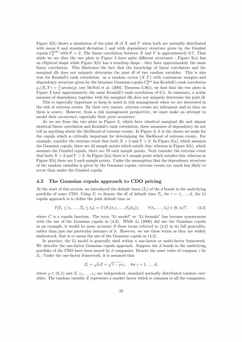
Figure 3(b) shows a simulation of the joint df of X and Y when both are normally distributedwith mean 0 and standard deviation 1 and with dependency structure given by the Gumbelcopula Cgum
θ with θ := 2. The linear correlation between X and Y is approximately 0.7. Thuswhile we see that the two plots in Figure 3 have quite different structures - Figure 3(a) hasan elliptical shape while Figure 3(b) has a teardrop shape - they have approximately the samelinear correlation. This illustrates the fact that the knowledge of linear correlation and themarginal dfs does not uniquely determine the joint df of two random variables. This is alsotrue for Kendall’s rank correlation: as a random vector (X,Y ) with continuous margins anddependency structure given by the bivariate Gaussian copula Cgau
ρ has Kendall’s rank correlation
ρτ (X,Y ) = 2π arcsin(ρ) (see McNeil et al. (2005, Theorem 5.36)), we find that the two plots in
Figure 3 have approximately the same Kendall’s rank correlation of 0.5. In summary, a scalarmeasure of dependency together with the marginal dfs does not uniquely determine the joint df.
This is especially important to keep in mind in risk management when we are interested inthe risk of extreme events. By their very nature, extreme events are infrequent and so data onthem is scarce. However, from a risk management perspective, we must make an attempt tomodel their occurrence, especially their joint occurence.
As we see from the two plots in Figure 3, which have identical marginal dfs and almostidentical linear correlation and Kendall’s rank correlation, these measures of dependency do nottell us anything about the likelihood of extreme events. In Figure 3, it is the choice we make forthe copula which is critically important for determining the likelihood of extreme events. Forexample, consider the extreme event that both X > 2 and Y > 2. In Figure 3(a), which assumesthe Gaussian copula, there are 43 sample points which satisfy this, whereas in Figure 3(b), whichassumes the Gumbel copula, there are 70 such sample points. Next consider the extreme eventthat both X > 3 and Y > 3. In Figure 3(a) there is 1 sample point which satisfies this, whereas inFigure 3(b) there are 5 such sample points. Under the assumption that the dependency structureof the random variables is given by the Gaussian copula, extreme events are much less likely tooccur than under the Gumbel copula.
4.3 The Gaussian copula approach to CDO pricing
At the start of this section, we introduced the default times (Ti) of the d bonds in the underlyingportfolio of some CDO. Using Fi to denote the df of default time Ti, for i = 1, . . . , d, the Licopula approach is to define the joint default time as
P[T1 ≤ t1, . . . , Td ≤ td] := C(F1(t1), . . . , Fd(td)), ∀(t1, . . . , td) ∈ [0,∞)d, (4.2)
where C is a copula function. The term “Li model” or “Li formula” has become synonymouswith the use of the Gaussian copula in (4.2). While Li (2000) did use the Gaussian copulaas an example, it would be more accurate if these terms referred to (4.2) in its full generality,rather than just one particular instance of it. However, we use these terms as they are widelyunderstood, that is to mean the use of the Gaussian copula in (4.2).
In practice, the Li model is generally used within a one-factor or multi-factor framework.We describe the one-factor Gaussian copula approach. Suppose the d bonds in the underlyingportfolio of the CDO have been issued by d companies. Denote the asset value of company i byZi. Under the one-factor framework, it is assumed that
Zi =√ρZ +
√1− ρ εi, for i = 1, . . . , d,
where ρ ∈ (0, 1) and Z, ε1, . . . , εd are independent, standard normally distributed random vari-ables. The random variable Z represents a market factor which is common to all the companies,
10
while the random variable εi is the factor specific to company i, for each i = 1, . . . , d. Under thisassumption, the transpose of the vector (Z1, . . . , Zd) is multivariate normally distributed withmean zero and with a covariance matrix whose off-diagonal elements are each equal to ρ. In thisframework, we interpret ρ as the correlation between the asset values of each pair of companies.
The idea is that default by company i occurs if the asset value Zi falls below some thresh-old value. The default time Ti is related to the one-factor structure by the relationship Zi =Φ−1(Fi(Ti)). With this relationship, the joint df of the default times is given by (4.2), withC := Cgau
ρ , where ρ is the correlation between the asset values (Zi). Once we have chosen themarginal dfs (Fi), we have fully specified the one-factor Li model.
Often, the marginal dfs are assumed to be exponentially distributed. In that case, the meanof each default time Ti can be estimated from the market, for instance from historical defaultinformation or the market prices of defaultable bonds. Using these exponential marginal dfsand the market prices of CDO tranches, investors can calculate the implied asset correlationρ for each tranche. The implied asset correlation ρ is the asset correlation value which makesthe market price of the tranche agree with the one-factor Gaussian copula model. However,as we also mention in Subsection 5.2, this results in asset correlation values which differ acrosstranches.
4.4 Credit default swaps and synthetic CDOs
The Li model can be used not only to value the CDOs we described in Section 3, but also anothertype of credit derivative called a credit defaut swap (“CDS”). A CDS is a contract which transfersthe credit risk of a reference entity, such as a bond or loan, from the buyer of the CDS to theseller. The buyer of the CDS pays the seller a regular premium. If a credit event occurs, forexample the reference entity becomes bankrupt or undergoes debt restructuring, then the sellerof the CDS makes an agreed payoff to the buyer. What constitutes a credit event, the payoffamount and how the payoff is made is set out in the legal documentation accompanying theCDS.
There are two categories of CDSs: a single-name CDS, which protects against credit eventsof a single reference entity, and a multi-name CDS, which protects against credit events in a poolof reference entities. In the market, a CDS is quoted in terms of a spread. The spread is thepremium payable by the buyer to the seller which makes the present value of the contract equalto zero. Roughly, a higher spread indicates a higher credit risk.
The market for CDSs is large. The Bank of International Settlements Quarterly Review ofJune 2009 gives the value of the notional amount of outstanding CDSs as US$42,000 billion as atDecember 31 2008, of which roughly two-thirds were single-name CDSs. Even after calculatingthe net exposure, this still corresponds to an amount above US$3,000 billion.
As CDSs grew in popularity, the banks which sold them ended up with many single-nameCDSs on their books. The banks grouped together many single-name CDSs and used them asthe underlying portfolio of a type of CDO called a synthetic CDO. In contrast, the cash CDOs wedescribed in Section 3 have more traditional assets like loans or bonds in the underlying portfolio.As an indication of the market size for these instruments just prior to the Crisis, the SecuritiesIndustry and Financial Markets Association gives the value of cash CDOs issued globally in 2007as US$340 billion and the corresponding value for synthetic CDOs as US$48 billion. It is alsoimportant to point out that products like CDOs and CDSs are currently not traded in officiallyregulated markets, but are traded over-the-counter (“OTC”). The global OTC derivative marketis of a staggering size, with a nominal, outstanding value at the end of 2008 of US$592,000 billion;see BIS (2009). To put this amount into perspective, the total GDP for the world in 2008 wasabout US$61,000 billion.
11

Just like any CDO, a synthetic CDO can be tranched and the tranches sold to investors.The buyers of the tranches receive a regular premium and, additionally, the buyers of the equitytranche receives an upfront fee. This upfront fee can be of the order 20%-50% of the nominalvalue of the underlying portfolio.
There also exists synthetic CDO market indices, such as the Dow Jones’ CDX family and theInternational Index Company’s iTraxx family, which are actively traded as contracts paying aspecified premium. These standardized market indices mean that there is a market-determinedprice for the tranches, which is expressed in terms of a spread for each tranche, in addition toan upfront fee for the equity tranche.
5 The drawbacks of the copula-based model in credit risk
The main use of the Gaussian copula model was originally for pricing credit derivatives. However,as credit derivative markets have grown in size, the need for a model for pricing has diminished.Instead, the market determines the price. However, the model is still used to determine abenchmark price and also has a significant role in hedging tranches of CDOs; see Finger (2009).Moreover, it is still widely used for pricing synthetic CDOs.
The model has some major advantages, which have for many people in industry outweighedits rather significant disadvantages, a story that we have most unfortunately been hearing fartoo often in risk management. Think of examples like the Black-Scholes-Merton model, or thewidespread use of Value-at-Risk (“VaR”) as a measure for calculating risk capital. All of theseconcepts have properties which need to be well understood by industry, especially when marketsof the size encountered in credit risk are built upon them.
But first to the perceived advantages of the Gaussian copula model. These are that it issimple to understand, it enables fast computations and it is very easy to calibrate since only thepairwise correlation ρ needs to be estimated. Clearly, the easy calibration by only one parameterrelies on the tenuous assumption that all the assets in the underlying portfolio have pairwise thesame correlation. The advantages of the model meant that it was quickly adopted by industry.For instance, by the end of 2004, the three main rating agencies - Fitch Ratings, Moody’s andStandard & Poor’s - had incorporated the model into their rating toolkit. Moreover, it is stillconsidered an industry standard.
Simplicity and ease of use typically comes at a price. For the Gaussian copula model, thereare three main drawbacks:
• insufficient modeling of default clustering in the underlying portfolio;
• if we calculate a correlation figure for each tranche of a CDO, we would expect these figuresto be the same. This is because we expect the correlation to be a function of the underlyingportfolio and not of the tranches. However, under the Gaussian copula model, the tranchecorrelation figures are not identical, and
• no modeling of the economic factors causing defaults weakens the ability to do stress-testing,especially on a company-wide basis.
We examine each of these issues in turn.
5.1 Inadequate modeling of default clustering
One of the main disadvantages of the model is that it does not adequately model the occurrenceof defaults in the underlying portfolio of corporate bonds. In times of crisis, corporate defaults
12
occur in clusters, so that if one company defaults then it is likely that other companies alsodefault within a short time period. Under the Gaussian copula model, company defaults becomeindependent as their size of default increases. Mathematically, we can illustrate this using theidea of tail dependence. A tail dependence measure gives the strength of dependence in the tails ofa bivariate distribution. We borrow heavily from McNeil et al. (2005) in the following exposition.Since dfs have lower tails (the left part of the df) and upper tails (the right part), we can define atail dependence measure for each one. Here, we consider only the upper tail dependence measure.Recall that the generalized inverse of a df F is defined by F←(y) := inf{x ∈ R : F (x) ≥ y}. Inparticular, if F is continuous and strictly increasing, then F← equals the ordinary inverse F−1
of F .
Definition 5.1. LetX and Y be random variables with dfs F andG, respectively. The coefficientof upper tail dependence of X and Y is
λu := λu(X,Y ) := limq→1−
P (Y > G←(q) |X > F←(q)) ,
provided a limit λu ∈ [0, 1] exists. If λu ∈ (0, 1] then X and Y are said to show upper taildependence. If λu = 0 then X and Y are said to be asymptotically independent in the uppertail.
It is important to realize that λu depends only on the copula C and not on the marginal dfsF and G; see McNeil et al. (2005, page 209).
Suppose X and Y have a joint df with Gaussian copula Cgauρ . As long as ρ < 1, it turns out
that the coefficient of upper tail dependence of X and Y equals zero; see McNeil et al. (2005,Example 5.32). This means that if we go far enough into the upper tail of the joint distributionof X and Y , extreme events appear to occur independently.
Recall that the dependence structure in the Li model is given by the Gaussian copula. Theasymptotic independence of extreme events for the Gaussian copula carries over to asymptotic in-dependence for default times in the Li model. If we seek to model defaults which cluster together,so that they exhibit dependence, the property of asymptotic independence is not desirable. Thisundesirable property of the Gaussian copula is pointed out in Embrechts et al. (2002) and wasexplicitly mentioned in the talk referred to at the beginning of Section 4. A first mathematicalproof is to be found in Sibuya (1960).
Compare the coefficient of upper tail dependence of the Gaussian copula with that of theGumbel copula. For X and Y with joint df given by Cgum
θ , the coefficient of upper tail dependence
is given by λgumu := 2−2
1θ . As long as θ > 1, then the Gumbel copula shows upper tail dependence
and may hence be more suited to modeling defaults in corporate bonds.In practice, as we do not take asymptotic limits, we wonder if the independence of the
Gaussian copula in the extremes only occurs in theory and is insignificant in practice. Theanswer is categorically no. As we pointed out in Subsection 4.2 in relation to Figure 3, theeffects of the tail independence of the Gaussian copula are seen not only in the limit. Of course,this is not a proof and we direct the reader to a more detailed discussion on this point in McNeilet al. (2005, page 212).
The Gumbel copula is not the only copula that shows upper tail dependence and we havechosen it simply for illustrative purposes. However, it demonstrates that alternatives to theGaussian copula do exist, as was pointed out in the academic literature on numerous occasions.For example, see Frey et al. (2001) and Rogge and Schonbucher (2003).
The failure of the Gaussian copula to capture dependence in the tail is similar to the failure ofthe Black-Scholes-Merton model to capture the heavy-tailed aspect of the distribution of equityreturns. Both the Gaussian copula and the Black-Scholes-Merton model are based on the normal
13
distribution. Both are easy to understand and result in models with fast computation times. Yetboth fail to adequately model the occurrence of extreme events.
We believe that it is imperative that the financial world considers what the model they useimplies about frequency and severity of extreme events. For managing risk, it is imprudent toignore the very real possibility of extreme events. It is unwise to rely without thought on a modelbased on the normal distribution to tell you how often these extreme events occur. We are notsuggesting that models based on the normal distribution should be discarded. Instead, theyshould be used in conjunction with several different models, some of which should adequatelycapture extreme events, and all of whose advantages and limitations are understood by thoseusing them and interpreting the results. Extreme Value Theory offers tools and techniques whichcan help in better understanding the problems and difficulties faced when trying to understand,for instance, joint extremes, market spillovers and systemic risk; see Coles (2001), Embrechtset al. (2008) and Resnick (2007) for a start.
5.2 Inconsistent implied correlation in tranches and an early warning
The one-factor Gaussian copula model is frequently used in practice for delta-hedging of theequity tranche of the synthetic CDO indices. Attracted by the high upfront fee, investors likehedge funds sell the equity tranche of a synthetic CDO. To reduce the impact of changes inthe spreads of the underlying portfolio, they can delta-hedge the equity tranche by buying acertain amount of the mezzanine tranche of the same index. The idea is that small losses in theequity tranche are offset by small gains in the mezzanine tranche and vice versa. They buy themezzanine tranche rather than the entire index because it is cheaper. Assuming the delta-hedgeworks as envisaged, the investor gains the high upfront fee and the regular premium payable onthe equity tranche they sold, less the regular premium payable on the mezzanine tranche theybought.
First, an implied correlation is calculated for each tranche. This is the correlation whichmakes the market price of the tranche agree with the one-factor Gaussian copula model. Usingthe implied correlations, the delta for each tranche can be calculated. The delta measuresthe sensitivity of the tranche to uniform changes in the spreads in the underlying portfolio.Intuitively, we would expect that the implied correlation should be the same for each tranche,since it is a property of the underlying portfolio. However, the one-factor Gaussian copula modelgives a different implied correlation for each tranche. Moreover, the implied correlations do notmove uniformly together since the implied correlation for the equity tranche can increase morethan the mezzanine tranche.
Even worse, sometimes it is not possible to calculate an implied correlation for a trancheusing the one-factor Gaussian copula model. Kherraz (2006) gives a theoretical example of thisand Finger (2009) gives the number of times that there has failed to be an implied correlation inthe marketplace. These are all serious drawbacks of the one-factor Gaussian copula model, whichwere brought to the attention of market participants in a dramatic fashion in 2005. Discussionsof these drawbacks can be found in Duffie (2008) and, particularly in relation to the events ofMay 2005 which we outline next, in Finger (2005) and Kherraz (2006).
In 2005, both Ford and General Motors were in financial troubles which threatened theircredit ratings. On May 4 2005, an American billionaire Kirk Kerkorian invested US$870 million inGeneral Motors. In spite of this, on May 5 2005, both Ford and General Motors were downgraded.Coming one day after Kerkorian’s massive investment, the downgrade was not expected by themarket. In the ensuing market turmoil, the mezzanine tranches moved in the opposite direction towhat the delta-hedgers expected. Rather than the delta-hedge reducing their losses, it increasedthem.
14
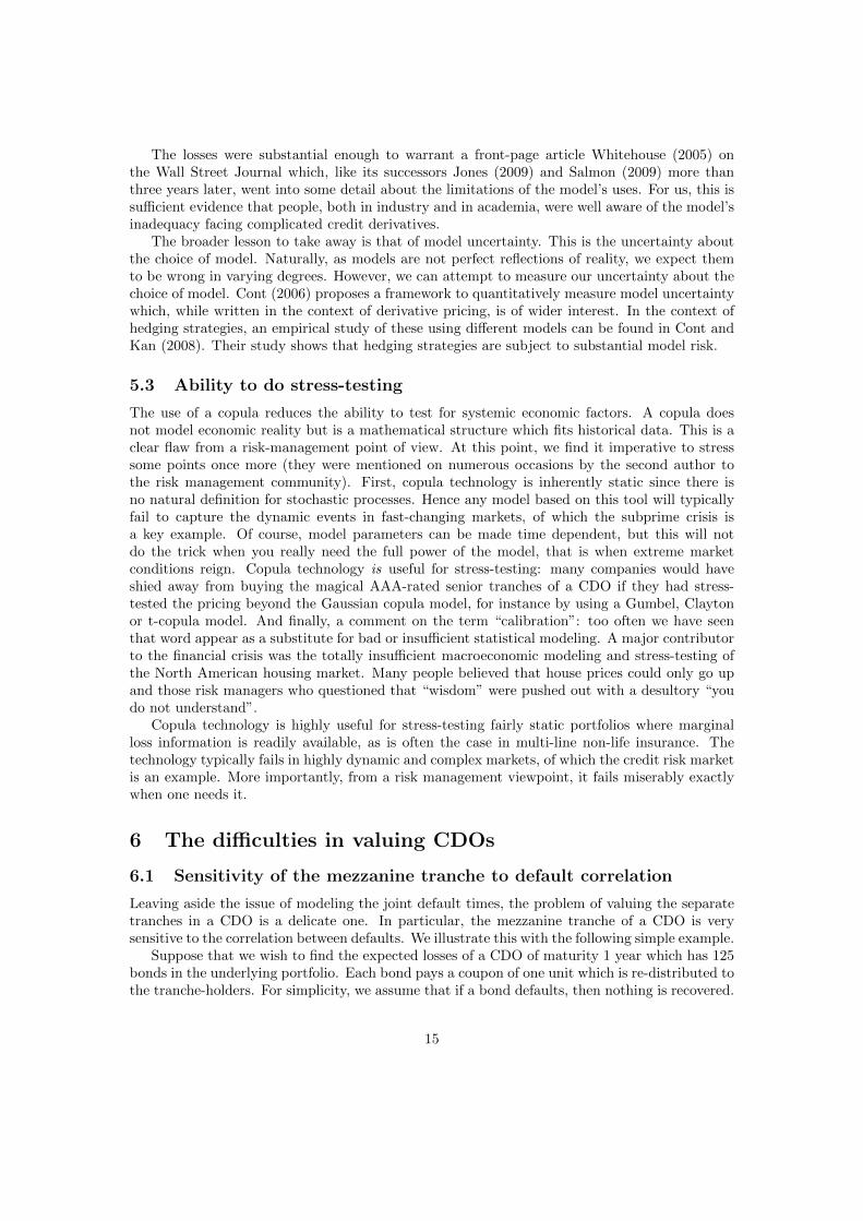
The losses were substantial enough to warrant a front-page article Whitehouse (2005) onthe Wall Street Journal which, like its successors Jones (2009) and Salmon (2009) more thanthree years later, went into some detail about the limitations of the model’s uses. For us, this issufficient evidence that people, both in industry and in academia, were well aware of the model’sinadequacy facing complicated credit derivatives.
The broader lesson to take away is that of model uncertainty. This is the uncertainty aboutthe choice of model. Naturally, as models are not perfect reflections of reality, we expect themto be wrong in varying degrees. However, we can attempt to measure our uncertainty about thechoice of model. Cont (2006) proposes a framework to quantitatively measure model uncertaintywhich, while written in the context of derivative pricing, is of wider interest. In the context ofhedging strategies, an empirical study of these using different models can be found in Cont andKan (2008). Their study shows that hedging strategies are subject to substantial model risk.
5.3 Ability to do stress-testing
The use of a copula reduces the ability to test for systemic economic factors. A copula doesnot model economic reality but is a mathematical structure which fits historical data. This is aclear flaw from a risk-management point of view. At this point, we find it imperative to stresssome points once more (they were mentioned on numerous occasions by the second author tothe risk management community). First, copula technology is inherently static since there isno natural definition for stochastic processes. Hence any model based on this tool will typicallyfail to capture the dynamic events in fast-changing markets, of which the subprime crisis isa key example. Of course, model parameters can be made time dependent, but this will notdo the trick when you really need the full power of the model, that is when extreme marketconditions reign. Copula technology is useful for stress-testing: many companies would haveshied away from buying the magical AAA-rated senior tranches of a CDO if they had stress-tested the pricing beyond the Gaussian copula model, for instance by using a Gumbel, Claytonor t-copula model. And finally, a comment on the term “calibration”: too often we have seenthat word appear as a substitute for bad or insufficient statistical modeling. A major contributorto the financial crisis was the totally insufficient macroeconomic modeling and stress-testing ofthe North American housing market. Many people believed that house prices could only go upand those risk managers who questioned that “wisdom” were pushed out with a desultory “youdo not understand”.
Copula technology is highly useful for stress-testing fairly static portfolios where marginalloss information is readily available, as is often the case in multi-line non-life insurance. Thetechnology typically fails in highly dynamic and complex markets, of which the credit risk marketis an example. More importantly, from a risk management viewpoint, it fails miserably exactlywhen one needs it.
6 The difficulties in valuing CDOs
6.1 Sensitivity of the mezzanine tranche to default correlation
Leaving aside the issue of modeling the joint default times, the problem of valuing the separatetranches in a CDO is a delicate one. In particular, the mezzanine tranche of a CDO is verysensitive to the correlation between defaults. We illustrate this with the following simple example.
Suppose that we wish to find the expected losses of a CDO of maturity 1 year which has 125bonds in the underlying portfolio. Each bond pays a coupon of one unit which is re-distributed tothe tranche-holders. For simplicity, we assume that if a bond defaults, then nothing is recovered.
15

We value the first three (most risky) CDO tranches, which we call the equity, mezzanine andsenior tranches. The equity tranche is exposed to the first 3 defaults in the underlying portfolioof bonds. The mezzanine tranche is exposed to the next 3 defaults and the senior tranche isexposed to the subsequent 3 defaults in the underlying portfolio of bonds. Therefore, 6 defaultsmust occur in the underlying portfolio before further defaults affect the coupon payments to thesenior tranche.
Instead of modeling the default times (Ti), we make the simple assumption that each ofthe underlying bonds has a fixed probability of defaulting within a year. We assume that thecorrelation between each pair of default events is identical. We calculate the expected loss oneach tranche at the end of the year as follows
Expected loss on equity tranche =
3∑k=1
kP [k bonds default by the end of the year] ,
Expected loss on mezzanine tranche =
3∑k=1
kP [k + 3 bonds default by the end of the year] ,
Expected loss on senior tranche =
3∑k=1
kP [k + 6 bonds default by the end of the year] .
In Figures 4(a)-4(d), we show for various probabilities of default how the expected losses on eachtranche vary as we change the pairwise correlation between the default events.
For each plot, we see that the expected loss on the equity tranche decreases as the pairwisecorrelation increases. The reason is that as correlation increases, it is more likely that eithermany bonds default or many bonds do not default. Since any defaults cause losses on theequity tranche, the increase in probability that many defaults do not occur tends to decreasethe expected loss on the equity tranche. Conversely, the expected loss on the senior trancheincreases as the pairwise correlation increases. More than 6 bonds must default before the seniortranche suffers a loss. An increase in correlation makes it more likely that many bonds willdefault and this causes the expected loss on the senior tranche to increase. However, for themezzanine tranche there is no clear relationship emerging. In Figure 4(a), the expected loss onthe mezzanine tranche increases as the pairwise correlation increases. But in Figure 4(d) theopposite happens. This simple example illustrates the sensitivity of the mezzanine tranche. Thispoint is also highlighted by McNeil et al. (2005, Figure 9.3).
We restate the remark in Duffie (2008) that the modeling of default correlation is currentlythe weakest link in the risk measurement and pricing of CDOs. Given this weakness and thesensitivity of the mezzanine tranche to the default correlation, it is clear that there is a lot ofuncertainty in the valuation of CDOs. Linking this uncertainty to the astronomical volumes ofCDOs in the marketplace, it is not surprising that the credit crisis had to erupt eventually.
6.2 Squaring the difficulty: CDO-squared
Now suppose we wish to value a credit derivative called a CDO-squared. This is a CDO wherethe underlying portfolio itself consists of CDO tranches. Moreover, these tranches are typicallythe mezzanine tranches. This is because the mezzanine tranches are difficult to sell: they aretoo risky for many investors, since they are often BBB-rated, yet they are not risky enough forother investors, like hedge funds.
Like any CDO, the CDO-squared can be tranched. However, the valuation of the CDO-squared and its tranches are fraught with complexity. As we saw in our simple example above,
16
0.00 0.01 0.02 0.03 0.04 0.05
0.0
0.5
1.0
1.5
2.0
2.5
3.0
Pairwise correlation
Exp
ecte
d lo
ss o
n tr
anch
e
●●
● ● ● ● ● ● ● ● ● ● ● ● ● ● ● ● ● ● ●
●
EquityMezzanineSenior
(a) individual default probability of 1%.
0.00 0.01 0.02 0.03 0.04 0.05
0.0
0.5
1.0
1.5
2.0
2.5
3.0
Pairwise correlation
Exp
ecte
d lo
ss o
n tr
anch
e
●●
● ● ● ● ● ● ● ● ● ● ● ● ● ● ● ● ● ● ●
●
EquityMezzanineSenior
(b) individual default probability of 2%.
0.00 0.01 0.02 0.03 0.04 0.05
0.0
0.5
1.0
1.5
2.0
2.5
3.0
Pairwise correlation
Exp
ecte
d lo
ss o
n tr
anch
e
● ● ● ● ● ● ● ● ● ● ● ● ● ● ● ● ● ● ● ● ●
●
EquityMezzanineSenior
(c) individual default probability of 3%.
0.00 0.01 0.02 0.03 0.04 0.05
0.0
0.5
1.0
1.5
2.0
2.5
3.0
Pairwise correlation
Exp
ecte
d lo
ss o
n tr
anch
e
●●
●●
●● ● ● ● ● ● ● ● ● ● ● ● ● ● ● ●
●
EquityMezzanineSenior
(d) individual default probability of 4%.
Figure 4: Expected loss on a CDO with 125 underlying names, each with identical pairwisecorrelation, as a function of the pairwise correlation value. The line shows the expected loss onthe equity tranche (0−3 units of exposure). The circles show the expected loss on the mezzaninetranche (3 − 6 units of exposure) and the crosses show the expected loss on the senior tranche(6− 9 units of exposure).
17
valuing each mezzanine tranche in the underlying portfolio is difficult. Valuing the tranches of theCDO-squared, which has between 100 and 200 mezzanine tranches in the underlying portfolio,is much more difficult. If we assume that there are 150 mezzanine tranches in the underlyingportfolio of the CDO-squared, and each mezzanine tranche is based on a portfolio of 150 bonds,then this means modeling 22,500 bonds. It is also quite likely that some of these bonds are thesame, since it is likely given the large numbers involved that some of the mezzanine tranches havethe same bonds in their underlying portfolio. Given these problems, it is questionable whethera CDO-squared can be valued with any reasonable degree of accuracy.
Moreover, doing due diligence on such on a CDO-squared is not feasible, as Haldane (2009a)points out. The contracts governing each of the mezzanine tranches in the underlying portfolioare around 150 pages long. Assuming that there are 150 mezzanine tranches in the underlyingportfolio, this means that there are 22,500 pages to read, not including the contract governingthe CDO-squared itself. On top of that, a typical computer program mapping the cashflow ofjust one CDO-like structure can be thousands of lines of computer code long (often in an Excelenvironment), which has the attendant possibility of programming errors creeping in.
For the purposes of risk management, determining the systemic factors which the CDO-squared is exposed to would be impossible, given the number of financial instruments on whicha CDO-squared is based. This means that the validity of scenario testing on such instruments isdoubtful.
Even ignoring the valuation difficulties, the economic value of instruments such as CDOs-squared are questionable. As Hellwig (2009, page 153) argues in relation to mortgage-backedsecurities, which we recall are a type of CDO, if the securitization of mortgage-backed securitieshad been properly handled then there should be no significant benefits from additional diversifi-cation through a mortgage-backed security-squared. Such benefits could be gained by investorsputting multiple mortgage-backed securities into their own portfolio. Furthermore, he points outthat the scope for moral hazard was increased as the chain of financial intermediation increased,from the mortgage originators to the buyers of the mortgage-backed security-squared. This wasalso mentioned by Stiglitz (2008).
If the problems with valuing and managing the risk involved in CDOs-squared seem insur-mountable, it should give the reader pause for thought that instruments called CDO-cubed exist.These are again CDOs which are based on the mezzanine tranches of CDO-squareds.
It is clear that at this level, credit risk management did reach a level of perversity which ques-tions seriously any socio-economic benefit of such products and puts to shame the whole quantprofession. In the end, from a product development point-of-view, total opaqueness reigned. Thereal question is not about a particular model used or misused in the pricing of such products butmuch more about the market structures which allowed such nonsensical products to be launchedin such volumes. Already around 2005, it was noticed that overall risk capital as measured byVaR was down. They key question some risk managers asked was “But where is all the creditrisk hiding?” By now, unfortunately we know!
7 Alternative approaches to valuing CDOs
Reading the articles in the Financial Times and Wired Magazine, one would think that theGaussian copula model was the only method used to value credit derivatives. This is far fromthe truth. While this model is widely used, there are many alternatives to it which are alsoused in industry. In fact, there are entire books written on models for credit derivatives, such asBielecki and Rutkowski (2004), Bluhm and Overbeck (2007), O’Kane (2008) and Schonbucher(2003).
18

Broadly, there are two main classes of models used in credit risk modeling: structural modelsand hazard rate models. The structural approach, sometimes called the firm-value approach,models default via the dynamics of the value of the firm. This is based on the Merton (1974)approach, which models default via the relationship of the value of the firm’s assets to its liabilitiesat the end of a given time period. The general idea is that default occurs if the asset value is lessthan the firm’s liabilities. The one-factor Gaussian copula model is an example of a structuralmodel. Other examples of structural models used in industry are the CreditMetrics model,publicized by JP Morgan in 1997, and the KMV model, first developed by the company KMVand now owned by Moody’s.
Hazard rate models, also commonly called reduced-form models, attempt to model the in-finitesimal chance of default. In these models, the default is some exogenous process which doesnot depend on the firm. An industry example of a reduced-form model is CreditRisk+, whichwas proposed by Credit Suisse Financial Products in 1997.
We do not go into details about these or, indeed, alternative models. Instead, as a startingpoint we direct the interested reader to the books cited at the start of this section.
It is fair to say that in the wake of the Crisis, the approaches used by the various marketparticipants to value CDOs can be broadly summarized as follows:
• for synthetic (corporate credit) CDOs, the notion of the base correlation curve of theGaussian copula is used. Since the Crisis, there has been an evolution to simpler modelsand simpler structures;
• for cash CDOs and asset-backed securities, a more detailed modeling of the cashflow wa-terfall together with Monte Carlo modeling of the underlying asset pools is used;
• rating agencies models for structured assets have become much simpler, that is concentrat-ing on fewer scenarios with extreme stress shocks, and
• the regulators put a lot of importance on stress-testing and the Holy Grail still remainsliquidity risk.
Whereas we applaud the consensus on simple, economically relevant products, we are less con-vinced that simple models will be part of the answer to this Crisis. Even for fairly straightforwardcredit products, rather advanced quantitative techniques are needed. We need better models andfor people to understand the assumptions and limitations of the models they use. The call isnot for “less mathematics” but rather for “a better understanding of the necessary mathematicsinvolved”.
8 A failure of risk management: AIG
CDSs have also attracted a lot of attention with respect to the financial crisis, particularlyin association with the insurance company AIG. In September 2008, AIG was on the verge ofbankruptcy due to cashflow problems stemming from its CDS portfolio, before being saved by theUS government. We explain below how AIG came close to bankruptcy and draw some relevantlessons from their risk management failures.
8.1 The AIG story
The sad story of AIG, a company of around 100,000 employees brought to its knees by a smallsubsidiary of 400 employees, is an example of a failure of risk management, both at the divisionand the group level. AIG almost went bankrupt because it ran out of cash. We do not concern
19
ourselves here with regulation, but focus on the risk management side of the AIG story. Asummary of the AIG bailout by Sjostrom (2009) is well-worth reading, and this is the basis ofwhat we write below about AIG. We have supplemented this with other sources, mainly fromAIG regulatory filings and statements submitted to a US Senate Committee hearing on AIG.
AIG is a holding company which, through its subsidiaries, is engaged in a broad range ofinsurance and insurance-related activities in more than 130 countries. Half of its revenues comefrom its US operations. As at December 31 2007, AIG had assets of US$1,000 billion dollars.This is just under half the Gross Domestic Product of France.
Despite the insurance business being a heavily regulated business, in September 2008 AIGwas on the verge of bankruptcy due to cashflow problems. These cashflow problems came notfrom its insurance business, but from its CDS portfolio. AIG operated its CDS business throughsubsidiaries called AIG Financial Products Corp and AIG Trading Group, Inc and their respectivesubsidiaries. Collectively, these subsidiaries are referred to as AIGFP. As the parent company,AIG fully guaranteed any liabilities arising from AIGFP doing its regular business. For the mostpart, AIGFP sold protection on super-senior tranches of CDOs, where the underlying portfolioconsisted of loans, debt securities, asset-backed securities and mortgage-backed securities. Super-senior tranches rank above AAA-rated tranches in the CDO tranche hierarchy, so that the super-senior tranche of a CDO is less risky than the AAA-rated tranche.
AIGFP believed that the money it earned from the CDSs were a free lunch because their riskmodels indicated that the underlying securities would never go into default. AIG (2006) statesthat “the likelihood of any payment obligation by AIGFP under each transaction is remote, evenin severe recessionary market scenarios”. The New York Times quotes the head of AIGFP assaying in August 2007 that “it is hard for us, without being flippant, to even see a scenario withinany kind of realm of reason that would see us losing one dollar in any of those transactions.”; seeMorgenson (2008). Indeed, as at March 5 2009, according to AIG’s primary regulator, there hadbeen no credit losses on the CDSs sold on super-senior tranches of CDOs; see Polakoff (2009).By credit losses, we mean the losses caused by defaults on the super-senior tranches that theCDSs were written on. Despite this, by writing the CDSs, AIGFP and hence also AIG, exposedthemselves to other risks which entailed potentially large financial obligations.
The buyer of a CDS is exposed to the credit risk of the seller. If the reference asset defaultsthen there is no guarantee that the seller can make the agreed payoff. Similarly, the selleris exposed to the credit risk of the buyer: the buyer may fail to make the regular premiumpayments. To reduce this risk, the counterparties to the CDS contract may be required topost collateral. The industry standard documentation which governs CDSs is produced by theInternational Swaps and Derivatives Association (“ISDA”). There are four parts to each ISDAcontract, the main part being the ISDA Master Agreement. Another of these parts is the CreditSupport Annex, which regulates the collateral payments. Collateral payments may be requireddue to changes in the market value of the reference asset or changes in the credit rating of thecounterparties. Further, the Credit Support Annex is an optional part of the ISDA contract.
As at December 31 2007, the net notional amount of CDSs sold by AIGFP was US$527 billion.The majority of these CDSs were sold before 2006. Some US$379 billion of these CDSs were soldto provide mostly European banks with regulatory capital relief, rather than for risk transfer.We call these “regulatory capital CDSs”. These CDSs were written on assets like corporateloans and prime residential mortgages, which were held by European banks. By buying a CDSfrom AIGFP, the banks transferred the credit risk of the loans to AIGFP. Up to 2005, as AIGwas AAA-rated and fully guaranteed its subsidiary AIGFP, the European banks were permittedunder their banking regulations to reduce the amount of regulatory capital to be set aside fortheir loans. Meanwhile AIG, being subject to different regulations and despite being exposed tothe losses on the loans, did not have to hold the full value of the European regulatory capital.
20
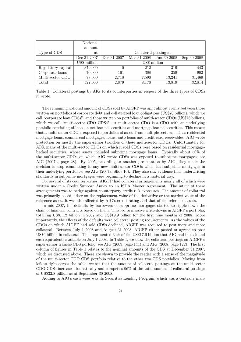
Notionalamount
Type of CDS at Collateral posting atDec 31 2007 Dec 31 2007 Mar 31 2008 Jun 30 2008 Sep 30 2008US$ million US$ million
Regulatory capital 379,000 0 212 319 443Corporate loans 70,000 161 368 259 902Multi-sector CDO 78,000 2,718 7,590 13,241 31,469Total 527,000 2,879 8,170 13,819 32,814
Table 1: Collateral postings by AIG to its counterparties in respect of the three types of CDSsit wrote.
The remaining notional amount of CDSs sold by AIGFP was split almost evenly between thosewritten on portfolios of corporate debt and collaterized loan obligations (US$70 billion), which wecall “corporate loan CDSs”, and those written on portfolios of multi-sector CDOs (US$78 billion),which we call “multi-sector CDO CDSs”. A multi-sector CDO is a CDO with an underlyingportfolio consisting of loans, asset-backed securities and mortgage-backed securities. This meansthat a multi-sector CDO is exposed to portfolios of assets from multiple sectors, such as residentialmortgage loans, commercial mortgages, loans, auto loans and credit card receivables. AIG wroteprotection on mostly the super-senior tranches of these multi-sector CDOs. Unfortunately forAIG, many of the multi-sector CDOs on which it sold CDSs were based on residential mortgage-backed securities, whose assets included subprime mortgage loans. Typically about 50% ofthe multi-sector CDOs on which AIG wrote CDSs was exposed to subprime mortgages; seeAIG (2007b, page 28). By 2005, according to another presentation by AIG, they made thedecision to stop committing to any new multi-sector CDOs which had subprime mortgages intheir underlying portfolios; see AIG (2007a, Slide 16). They also saw evidence that underwritingstandards in subprime mortgages were beginning to decline in a material way.
For several of its counterparties, AIGFP had collateral arrangements nearly all of which werewritten under a Credit Support Annex to an ISDA Master Agreement. The intent of thesearrangements was to hedge against counterparty credit risk exposures. The amount of collateralwas primarily based either on the replacement value of the derivative or the market value of thereference asset. It was also affected by AIG’s credit rating and that of the reference assets.
In mid-2007, the defaults by borrowers of subprime mortgages started to ripple down thechain of financial contracts based on them. This led to massive write-downs in AIGFP’s portfolio,totalling US$11.2 billion in 2007 and US$19.9 billion for the first nine months of 2008. Moreimportantly, the effects of the defaults were collateral posting requirements. As the values of theCDOs on which AIGPF had sold CDSs declined, AIGFP was required to post more and morecollateral. Between July 1 2008 and August 31 2008, AIGFP either posted or agreed to postUS$6 billion in collateral. This represented 34% of the US$17.6 billion that AIG had in cash andcash equivalents available on July 1 2008. In Table 1, we show the collateral postings on AIGFP’ssuper-senior tranche CDS porfolio; see AIG (2009, page 144) and AIG (2008, page 122). The firstcolumn of figures in Table 1 relates to the nominal amounts of the CDS at December 31 2007,which we discussed above. These are shown to provide the reader with a sense of the magnitudeof the multi-sector CDO CDS portfolio relative to the other two CDS portfolios. Moving fromleft to right across the table, we see that the amount of collateral postings on the multi-sectorCDO CDSs increases dramatically and comprises 96% of the total amount of collateral postingsof US$32.8 billion as at September 30 2008.
Adding to AIG’s cash woes was its Securities Lending Program, which was a centrally man-
21

aged program facilitated by AIG Investments. Through this program, certain of AIG’s insurancecompanies lent securities to other financial institutions, primarily banks and brokerage firms. Inexchange, AIG received partially cash collateral equal to 102% of the fair value of the loanedsecurities from the borrowers. In 2008, as the borrowers learned of AIG’s cashflow problems,they asked for their collateral back in exchange for the return of the securities. From September12 2008 to September 30 2008, borrowers demanded the return of around US$24 billion in cash;see Dinallo (2009).
A typical securities lending program reinvests the collateral in short duration instrumentssuch as treasuries and commercial paper. AIG’s Securities Lending Program did not do this.Instead, they invested most of the collateral in longer duration, AAA-rated residential mortgage-backed securities; see AIG (2008, page 108) and Dinallo (2009). As the effects of the defaults ofsubprime mortgage holders continued to ripple through the financial markets, these mortgage-backed securities declined substantially in value and became illiquid. As a result, the SecuritiesLending Program had insufficient funds to pay back the collateral it had taken in exchange forlending AIG’s securities. AIG was forced to transfer billions in cash to the Securities LendingProgram to pay back the collateral.
By early September 2008, AIG’s cash situation was dire. It was unable to raise additionalcapital due to the seizing up of liquidity in the markets. As a result of all these events, AIG wasdowngraded. The downgrade triggered additional collateral postings in excess of US$20 billionon the CDSs sold by AIGFP.
On September 16 2008, the Federal Reserve Board, with the support of the U.S. Departmentof the Treasury, announced that it had authorized the Federal Reserve Bank of New York tolend up to US$85 billion to AIG. This was to allow AIG to sell certain of its businesses in anorderly manner, with the least possible disruption to the overall economy. According to a FederalReserve Board press release, it had determined that, in the current circumstances, a disorderlyfailure of AIG could add to already significant levels of financial market fragility and lead tosubstantially higher borrowing costs, reduced household wealth, and materially weaker economicperformance; see Federal Reserve Board (2008a). By October 1 2008, AIG had drawn downapproximately US$61 billion from the credit facility; see Kohn (2009).
In November 2008, it appeared that another downgrade of AIG’s credit rating was looming.This would have triggered additional collateral calls, and would probably have led to the collapseof AIG. Wishing to avoid this, the Federal Reserve Board and the U.S. Department of theTreasury announced a series of mitigating actions on November 10 2008; see Kohn (2009). Inthe press release, the Federal Reserve Board stated that these new measures were to establisha more durable capital structure, resolve liquidity issues, facilitate AIG’s execution of its planto sell certain of its businesses in an orderly manner, promote market stability, and protect theinterests of the US government and taxpayers; see Federal Reserve Board (2008b).
AIG’s net losses for 2008 were about US$99 billion, of which approximately US$62 billionwas in the last quarter of 2008. By August 2009, according to the magazine The Economist,the total value of US government help that was distributed to AIG was around US$145 billion,which is equivalent to about 1% of the GDP of the US.
8.2 Risk management issues
The risk management failings at AIG were seen at other global firms. For many firms, theshortcomings of the risk management practices were translated into huge financial losses. InAIG’s case, they almost bankrupted the firm.
The biggest failure of risk management at AIG was in not appreciating the risk inherent inthe super-senior tranches of the multi-sector CDOs. Indeed, Rutledge (2008) points to exposure
22

to the US subprime market as driving the losses at some major global financial organizations,with the key driver being exposure to the super-senior tranches of CDOs. Firms thought thatthe super-senior tranches were practically risk-free. According to Rutledge (2008), prior to thethird quarter of 2007, few firms used valuation models to model their exposure to super-seniortranches related to subprime mortgages. It seems that AIG was also guilty of this to some degree.Until 2007, it did not model the liquidity risk that it was exposed to from writing CDSs withcollateral posting provisions; see Mollenkamp et al. (2008) and St Denis (2008).
Inadequate mathematical modeling meant that AIG were not able to quantify properly therisks in their CDS portfolio. Moreover, by ignoring the liquidity risk they were exposed to untilafter the Crisis had begun, AIG could not take early action to reduce their exposure to potentialcollateral postings. By the end of 2007, when substantial declines in the subprime mortgagemarket were already occurring, it would have been very expensive to do this.
Some firms survived the Crisis better than others. Based on a sample of eleven global bankingorganizations and securities firms, Rutledge (2008) identified the key risk management practiceswhich differentiated the performance of firms during the Crisis. From them, we take some relevantlessons.
One is the need for firms to embrace quantitative risk management. This provides them witha means of quantifying and aggregating risks on a firm-wide basis. Relying on human judgment,while still essential, is not enough, especially in huge firms like AIG.
The mathematics to measure many of the risks that firms face are well-developed. For exam-ple, while the Crisis is considered an extreme event, there does exist a mathematical frameworkto assess the risk of such events. As mentioned before, Extreme Value Theory has been an activearea of mathematical research since the 1950s, with early publications going back to the 1920s,and has been applied to the field of finance for over 50 years. There has been much research onthe quantification of the interdependence and concentration of risks, and the aggregation of risks.A starting place for learning about the concepts and techniques of quantitative risk managementis McNeil et al. (2005).
9 Summary
The prime aim of this paper is not to give a detailed overview of all that went wrong leading upto and during the Crisis, but instead a rather personal account of the important issues of whichan actuarial audience should be aware. The pessimist may say “The only thing we learn fromhistory is that we learn nothing from history”, a quote attributed to Friedrich Hegel, amongothers. However, we hope that future generations of actuarial students will read this papereven after the Crisis has become part of economic history and avoid the errors of the currentgeneration. As a consequence, we have left out numerous important aspects of the Crisis, buthopefully we have compensated that oversight with some general references which we founduseful. By now, new publications appear every day which makes choosing “what to read” verydifficult indeed.
We have concentrated on two aspects of the Crisis which are relevant from an actuarialviewpoint: the use of an actuarial formula (that is, the Gaussian copula model) far beyond thelevel it was originally created for and the near-bankruptcy of an insurance giant, AIG, in partbecause of the failure of internal risk management practices.
If we consider the concepts behind the numerous acroynms like RM, IRM, ERM, QRM,...,the message is screaming out to us: we need to learn from these recent events. As stated onseveral occasions in our paper, it is totally preposterous to blame one man or one model for all orpart of the Crisis. In reaction to the Financial Times article Jones (2009) we wrote the following
23
letter:
Dear Sir
The article “Of couples and copulas”, published on 24 April 2009, suggests thatDavid Li’s formula is to blame for the current financial crisis. For me, this is akinto blaming Einstein’s E = mc2 formula for the destruction wreaked by the atomicbomb. Feeling like a risk manager whose protestations of imminent danger wereignored, I wish to make clear that many well-respected academics have pointed outthe limitations of the mathematical tools used in the finance industry, including Li’sformula. However, these warnings were either ignored or dismissed with a desultoryresponse: “It’s academic”.
We hope that we are listened to in the future, rather than being made a convenientscapegoat.
Yours, etc
It was unfortunately not published!As actuaries, both in practice and in academia, we must think more carefully on how to
communicate the use and potential misuse of the concepts, techniques and tools in use in therisk management world. Two things are clear from the Crisis: “we were not listened to”, but also“we did not know”. First on the latter: as academics, we have to become much more involvedwith macroeconomic reality. The prime example is the astronomical nominal value invested incredit derivatives and why our risk management technology did not have all the red warninglights flashing much earlier. Second, as a final remark, we want to say something on the former“we were not listened to”. This leads us to the problem of communication, a stage on whichactuaries are not considered the best actors. Too many papers are currently written, post-event,on “why we got into this mess”. We need to learn why certain warnings were not heeded. Belowwe give some personal recollections on this matter.
In 2001, the second author contributed to the 17 page document Danıelsson et al. (2001) whichwas mailed in the same year as an official reply to the Basel Committee in the wake of the newBasel II guidelines. The academic authors were a mixture of microeconomists, macroeconomists,econometricians and actuaries. Due to its relevance to the Crisis, we quote from the ExecutiveSummary:
It is our view that the Basel Committee for Banking Supervision, in its Basel IIproposals, has failed to address many of the key deficiencies of the global financialregulatory system and even created the potential for new sources of instability. . . .
• The proposed regulations fail to consider the fact that risk is endogenous. Value-at-Risk can destabilise an economy and induce crashes when they would nototherwise occur.
• Statistical models used for forecasting risk have been proven to give inconsis-tent and biased forecasts, notably under-estimating the joint downside risk ofdifferent assets. . . .
• Heavy reliance on credit rating agencies for the standard approach to credit riskis misguided as they have been shown to provide conflicting and inconsistentforecasts of individual clients’ creditworthiness. . . .
• Financial regulation is inherently procyclical. Our view is that this set of propos-als will, overall, exacerbate this tendency significantly. In so far as the purpose offinancial regulation is to reduce the likelihood of systemic crisis, these proposalswill actually tend to negate, not promote this useful purpose.
24
The introduction of Danıelsson et al. (2001) concludes with
Perhaps our most serious concern is that these proposals, taken altogether, will en-hance both the procyclicality of regulation and the susceptibility of the financialsystem to systemic crises, thus negating the central purpose of the whole exercise.Reconsider before it is too late.
The authors of Danıelsson et al. (2001) could not have been more forceful and explicit, and yet thereaction from the Basel Committee was basically nil. Along these lines, every beginning actuaryshould read Markopolos (2005). In this 2005 document addressed to the SEC, one of several byMarkopolos over the period 2000-2008, Markopolos proves that Madoff Investment Securities is aPonzi scheme, and yet the SEC did nothing. We do not enter into the reasons why this happened,but simply note that every quantitatively trained finance expert would have immediately reactedupon reading the very detailed and point-by-point accusation made in Markopolos (2005).
Though the above example is somewhat discouraging, we have to keep vigilant and commu-nicate in a forceful way those actuarial, technical findings which are of societal importance. Wecan do this through our publications, societies and conferences. A key research theme that wehave to address more explicitly going forward is that of model uncertainty. From a technicalperspective, this means explaining the precise conditions under which a particular model can beused. But at the same time, we have to be aware, or become aware, where and how these modelsare used in a non-trivial way.
It always pays to be be humble in the face of real application. Shakespeare’s Hamlet for-mulated this as follows: “There are more things in heaven and earth, Horatio, than are dreamtof in your philosophy.” New generations of actuarial students will have to use the tools andtechniques of quantitative risk management wisely in a world where the rules of the game willconstantly change. A message we would like to give them on this path is to be always scientif-ically critical, socially honest and to adhere to the highest ethical principles, especially in theface of temptation...which will come!
Acknowledgements
The authors would like to extend their gratitude to the organisers of the 39th InternationalASTIN Colloquium in Helsinki, June 1-4 2009, for having invited Paul Embrechts to presentan early version of this paper. Catherine Donnelly thanks RiskLab at ETH Zurich for financialsupport. Research was partially completed while Paul Embrechts was visiting the Institute ofMathematical Sciences, National University of Singapore in November-December 2009.
References
AIG (2006). 2006 Annual Report, March 1 2007.
AIG (2007a). Capital Markets. Investor Meeting - December 5, 2007. http://library.
corporate-ir.net/library/76/761/76115/items/272197/capital.pdf.
AIG (2007b). Residential Mortgage Presentation (Financial figures are as at June 30, 2007)August 9, 2007 (Revised as to slide 29). http://media.corporate-ir.net/media_
files/irol/76/76115/REVISED_AIG_and_the_Residential_Mortgage_Market_FINAL_
08-09-07.pdf.
AIG (2008). 2008 Annual Report, March 27 2009.
25
AIG (2009). SEC 10-Q filing at March 31 2009.
Bielecki, T. R. and Rutkowski, M. (2004). Credit Risk: Modeling, Valuation and Hedging.Springer.
BIS (2009). Bank for International Settlements Quarterly Review, September 2009.
Bluhm, C. and Overbeck, L. (2007). Structured Credit Portfolio Analysis, Baskets and CDOs.Chapman and Hall/CRC.
Brunnermeier, M. K. (2009). Deciphering the liquidity and credit crunch 2007-2008. Journal ofEconomic Perspectives, 23(1):77–100.
Coles, S. (2001). An Introduction to Statistical Modeling of Extreme Values. Springer.
Cont, R. (2006). Model uncertainty and its impact on the pricing of derivative instruments.Mathematical Finance, 16(3):519–547.
Cont, R. and Kan, Y. H. (2008). Dynamic hedging of portfolio credit derivatives. SSRN:http://ssrn.com/abstract=1349847.
Crouhy, M. G., Jarrow, R. A., and Turnbull, S. M. (2008). The subprime credit crisis of 07.Journal of Derivatives, 16(4):81–110.
Danıelsson, J., Embrechts, P., Goodhart, C., Keating, C., Muennich, F., Renault, O., and Shin,H. (2001). An academic response to Basel II. LSE Financial Markets Group. Special PaperNumber 130.
Dinallo, E. (2009). American International Group: Examining what went wrong, governmentintervention, and implications for future regulation. Committee on Banking, Housing, andUrban Affairs. United States Senate. March 5 2009. Statement of Superintendent Eric Di-nallo, New York State Insurance Department.
Duffie, D. (2008). Innovations in credit risk transfer: implications for financial stability. BISWorking Papers, Monetary and Economic Department. Number 255.
Embrechts, P. (2009). Copulas: a personal view. Journal of Risk and Insurance, 76(3):639–650.
Embrechts, P., Kluppelberg, C., and Mikosch, T. (2008). Modelling Extremal Events for Insur-ance and Finance. Springer.
Embrechts, P., McNeil, A. J., and Straumann, D. (2002). Correlation and dependence in riskmanagement: properties and pitfalls. In M. Dempster, editor, Risk Management: Value atRisk and Beyond, pages 176–223. Cambridge University Press. First appeared in 1998 as aRiskLab ETH Zurich report.
Federal Reserve Board (2008a). September 16 2008, Press Release.
Federal Reserve Board (2008b). November 10 2008, Press Release.
Finger, C. C. (2005). Eating our own cooking. RiskMetrics Group, Research Monthly.
Finger, C. C. (2009). Testing hedges under the standard tranched credit pricing model. Risk-Metrics Journal, 9(1).
26

Follmer, H. (2009). Alles richtig und trotzdem falsch? Anmerkungen zur Finanzkrise und zurFinanzmathematik. Preprint, Humboldt-Universitat, Berlin.
Frey, R., McNeil, A. J., and Nyfeler, M. A. (2001). Copulas and credit models. Risk, pages111–114.
Genest, C., Gendron, M., and Bourdeau-Brien, M. (2009). The advent of copulas in finance.European Journal of Finance, 15(7-8):609–618.
Haldane, A. G. (2009a). Rethinking the financial network. Speech delivered at the Finan-cial Student Association, Amsterdam. April 28 2009. http://www.bankofengland.co.uk/publications/speeches/2009/speech386.pdf.
Haldane, A. G. (2009b). Why banks failed the stress test. The basis for a speech given at theMarcus-Evans conference on Stress-Testing, 9-10 February 2009. February 13 2009. http://www.bankofengland.co.uk/publications/speeches/2009/speech374.pdf.
Hellwig, M. F. (2009). Systemic risk in the financial sector: an analysis of the subprime-mortgagefinancial crisis. De Economist, 157(2):129–207.
IMF (2006). Global Financial Stability Report. Market developments and issues. April 2006.World Economic and Financial Surveys.
Jones, S. (2009). Of couples and copulas: the formula that felled Wall St. April 24 2009, FinancialTimes.
Keys, B. J., Mukherjee, T., Seru, A., and Vig, V. (2008). Financial regulation and securitization.Evidence from subprime loans. Journal of Monetary Economics, 56(5):700–720.
Kherraz, A. (2006). The May 2005 correlation crisis: did the models really fail? PortugueseFinance Network, 4th Finance Conference, July 6-8 2006, Porto, Portugal. http://www.fep.up.pt/conferencias/pfn2006/Conference Papers/592.pdf.
Kohn, D. L. (2009). American International Group: Examining what went wrong, governmentintervention, and implications for future regulation. Committee on Banking, Housing, andUrban Affairs. United States Senate. March 5 2009. Statement of Donald L. Kohn, ViceChairman, Board of Governors of the Federal Reserve System.
Li, D. (2000). On default correlation: a copula function approach. Journal of Fixed Income,9(4):43–54.
Lohr, S. (2009). Wall Street’s math wizards forgot a few variables. September 12 2009, NewYork Times.
Markopolos, H. (2005). The world’s largest hedge fund is a fraud. November 7 2005. Submissionto the SEC.
McNeil, A. J., Frey, R., and Embrechts, P. (2005). Quantitative Risk Management. Concepts,Techniques, Tools. Princeton University Press.
Merton, R. C. (1974). On the pricing of corporate debt: the risk structure of interest rates.Journal of Finance, 29(2):449–470.
Mollenkamp, C., Ng, S., Pleven, L., and Smith, R. (2008). Behind AIG’s fall, risk models failedto pass real-world test. October 31 2008, Wall Street Journal.
27
Morgenson, G. (2008). Behind insurer’s crisis: blind eye to a web of risk. September 28 2008,New York Times.
Nelsen, R. B. (2006). An Introduction to Copulas. Springer, second edition.
O’Kane, D. (2008). Modelling Single-Name and Multi-Name Credit Derivatives. Wiley.
Polakoff, S. M. (2009). American International Group: Examining what went wrong, governmentintervention, and implications for future regulation. Committee on Banking, Housing, andUrban Affairs. United States Senate. March 5 2009. Statement of Scott M. Polakoff, ActingDirector, Office of Thrift Supervision.
Resnick, S. (2007). Extreme Values, Regular Variation, and Point Processes. Springer.
Rogers, L. C. G. (2009). Financial mathematics and the credit crisis. Document in response toquestions posed by Lord Drayson, UK Science and Innovation Minister.
Rogge, E. and Schonbucher, P. J. (2003). Modelling dynamic portfolio credit risk. Workingpaper.
Rutledge, W. L. (2008). Observations on risk management practices during the recent mar-ket turbulence. March 6 2008. Senior Supervisors Group. http://www.newyorkfed.org/newsevents/news/banking/2008/SSG_Risk_Mgt_doc_final.pdf.
Salmon, F. (2009). Recipe for disaster: the formula that killed Wall Street. February 23 2009,Wired Magazine.
Schonbucher, P. J. (2003). Credit Derivatives Pricing Models: Models, Pricing and Implementa-tion. Wiley.
Schweizer, B. and Sklar, A. (1983). Probabilistic Metric Spaces. Elsevier Science Publishing Co.
SEC (2008). Summary report of issues identified in the commission staff’s examinations of selectcredit rating agencies. July 8 2008, United States Securities and Exchange Commission.http://www.sec.gov/news/studies/2008/craexamination070808.pdf.
Sibuya, M. (1960). Bivariate extreme statistics. Annals of the Institute of Statistical Mathematics,11:195–210.
Sjostrom, Jr., W. K. (2009). The AIG bailout. Washington and Lee Law Review, 66:943–991.
St Denis, J. W. (2008). Letter to Chairman Henry A. Waxman and Ranking Member ThomasM. Davis III from Joseph W. St Denis. Letter provided by Joseph W. St Denis to theCommittee on Oversight and Government Reform, House of Representatives, USA, datedOctober 4 2008.
Stiglitz, J. E. (2008). It doesn’t take Nostradamus. The Economists’ Voice, 5(8). Article no. 1.
The Economist (2008). Confessions of a risk manager. August 7 2008.
Turner, J. A. (2009). The Turner Review. March 2009. Financial Services Authority, UK.http://www.fsa.gov.uk/pubs/other/turner_review.pdf.
Wallace, D. (2009). The Turner Review. Letter to Lord Turner, Financial Services Authority,UK. June 5 2009.
28

Whitehouse, M. (2005). Slices of risk: how a formula ignited market that burned some biginvestors. September 12 2005, Wall Street Journal.
Wolf, M. (2008). Regulators should intervene in bankers’ pay. January 15 2008, Financial Times.
CATHERINE DONNELLY (corresponding author)RiskLab, Department of Mathematics,ETH Zurich,CH-8092 Zurich,Switzerland.E-Mail: [email protected]
PAUL EMBRECHTSRiskLab, Department of Mathematics,ETH Zurich,CH-8092 Zurich,Switzerland.E-Mail: [email protected]
29


![The Devil is in the Tails: Fine-grained Classification in ... · VAN HORN, PERONA: THE DEVIL IS IN THE TAILS 3. task. The recent Pasadena Trees dataset [55] is the exception. Most](https://img.pdfslide.net/doc/110x75/5f3e7e5c34b53518a0469454/the-devil-is-in-the-tails-fine-grained-classiication-in-van-horn-perona.jpg)