Essays on

The Dimensions of Youth Unemployment in South Africa

In fulfilment of the requirements for a Doctor of Philosophy in Economics

Gareth Arthur Roberts

Supervised by

Aylit Tina Romm and Neil Andrew Rankin

1

Contents

Introduction ............................................................................................................................................................................... 3

References ......................................................................................................................................................................... 16

Chapter 1. Is there first order short term state dependence in unemployment among young South

Africans? ................................................................................................................................................................................. 22

Introduction ....................................................................................................................................................................... 23

State dependence in unemployment among youth .............................................................................................. 26

The data .............................................................................................................................................................................. 30

Descriptions of the data ................................................................................................................................................ 38

The econometric approach ........................................................................................................................................... 50

Results ................................................................................................................................................................................. 58

Discussion and conclusion ........................................................................................................................................... 80

References ......................................................................................................................................................................... 82

Appendix ............................................................................................................................................................................ 85

Chapter 2. Does a targeted wage subsidy voucher have an effect on the reservation wages of young

South Africans? ..................................................................................................................................................................... 95

Introduction ....................................................................................................................................................................... 96

The reservation wages of young South Africans ................................................................................................. 99

The data ............................................................................................................................................................................ 103

The econometric approach ......................................................................................................................................... 112

Results ............................................................................................................................................................................... 116

Discussion and conclusion ......................................................................................................................................... 130

References ....................................................................................................................................................................... 133

Appendix .......................................................................................................................................................................... 137

Chapter 3. Are young South Africans overly optimistic about their labour market prospects? .............. 159

Introduction ..................................................................................................................................................................... 160

Type uncertainty and optimism ................................................................................................................................ 162

The data ............................................................................................................................................................................ 167

Descriptions of the data .............................................................................................................................................. 176

The econometric approach ......................................................................................................................................... 186

Results ............................................................................................................................................................................... 190

Discussion and conclusion ......................................................................................................................................... 202

References ....................................................................................................................................................................... 204

Appendix .......................................................................................................................................................................... 208

Conclusion ............................................................................................................................................................................ 214

List of Tables and Figures ............................................................................................................................................. 217

2

Acknowledgements

Many people have assisted me throughout the development of this thesis. This is why I will

refer to “we”, “us”, and “our” thesis even though the views expressed in this thesis and any

mistakes are entirely my own. I would like to thank all of you. In particular I am grateful to

my supervisors Neil and Aylit. I am also grateful for the support from Volker and the

encouragement from my parents Gerald and Karen. Finally I would like to thank Danielle for

her support, patience, and sense of humour while I was working on my PhD.

Declaration

3

“Man is diminished if he lives without knowledge of his past; without hope of a future he

becomes a beast.” ― P.D. James

Introduction

Rising unemployment in South Africa since the end of Apartheid poses an immense challenge

to Nelson Mandela’s legacy. The literature on unemployment in South Africa suggests that

unemployment in this country is largely structural and that the solution to the problem

requires reforms that allow capital and labour to expand production into new markets (see

Fourie, 2011; Mariotti and Meinecke, 2014; and Hausmann and Klinger, 2008). Any social

compact in South Africa will nevertheless have to subsidise the large number of unskilled

workers that have been marginalised (Cichello, Leibbrandt, and Woolard, 2014). Indeed,

South Africa has one of the largest social protection programmes for a developing state

(Niño-Zarazúa, Barrientos, Hickey, and Hulme, 2012) and there is a large literature

demonstrating the effect of social grants on the wellbeing of the poor (Aguero, Carter, and

Woolard, 2006). There are however studies that suggest that one of the unintended

consequences of these interventions is that they may contribute to unemployment (Bertrand,

Mullainathan, and Miller, 2003; and Abel, 2013).

Little is known about how to facilitate employment amongst the majority of unemployed

South Africans. There is evidence showing that investments in infrastructure have led to

higher levels of employment in rural areas (Dinkelman, 2011). It is unclear though if the

resources that were allocated to various economic development interventions since 1994

could have been used more efficiently. For example Dinkelman and Ranchhod (2012) show

that the introduction of minimum wage regulation for domestic workers had no statistically

significant effects on employment. Magruder (2012) in contrast shows that centralised

bargaining agreements have reduced employment in small firms.

4

Labour market data for South Africa nevertheless shows us that successive birth-cohorts are

confronted with a more competitive labour market than their predecessors (Branson,

Ardington, Lam, and Leibbrandt, 2013) despite leaving school with higher levels of education

(at least on paper). This leads to one of the central questions regarding the problem of

unemployment in South Africa: Should policy-makers be targeting the new entrants to the

labour force, the many older workers that are unemployed, or both – if young workers are

more likely to be unemployed1?

In one of the first economic studies to probe youth unemployment Freeman and Wise (1982)

highlight several features that differentiate youth unemployment from unemployment among

older workers (in the United States). Younger workers are more likely to switch between

searching for work and non-economic activities such as education, and they are prone to

being discouraged or less active job seekers. They offer several explanations for the causes of

youth unemployment including the general level of aggregate demand in the economy and the

proportion of young people in the population. There is a positive correlation between higher

levels of education and both employment and wages and they find evidence that young

workers from poor families experience higher rates of unemployment. Freeman and Wise

(1992) believe that youth unemployment is a concern not only because of the immediate

social and psychological effects of inactivity but also because, while a long spell of

1 Wainer, Palmer, and Bradlow (1998: 4-5) relate one of the first examples of the use of selection on

unobservables in policy: “Abraham Wald in some work he did during World War II (Mangel and Samaniego 1984;

Wald 1980) was trying to determine where to add extra armor to planes on the basis of the pattern of bullet holes

in returning aircraft. His conclusion was to determine carefully where returning planes had been shot and put

extra armor every place else! Wald made his discovery by drawing an outline of a plane… and then putting a mark

on it where a returning aircraft had been shot. Soon the entire plane had been covered with marks except for a few

key areas. It was at this point that he interposed a model for the missing data, the planes that did not return. He

assumed that planes had been hit more or less uniformly, and hence those aircraft hit in the unmarked places had

been unable to return, and thus those were the areas that required more armor. Wald's key insight was his model

for the nonresponse. From his observation that planes hit in certain areas were still able to return to base, Wald

inferred that the planes that didn't return must've been hit somewhere else.”

5

unemployment following the completion of school has no effect on employment probabilities

more than three years later, such unemployment is associated with a sizable negative effect on

wages later in life.

A second volume explores the “The Black Youth Employment Crisis” in the United States

(Freeman and Holzer, 1986). This study finds that there is no single factor that causes the

large difference in employment among black and white youth. Freeman and Holzer (1986: 8)

find that while it is more difficult for black youth to find work they are also more likely to

lose their jobs and that “survey responses to questions about the allocation of time show that

those out of school spent only 17 percent of their time on anything that could be considered

socially useful. The bulk of their days was instead spent watching television, going to movies,

listening to music, or the like, in other words, on ‘‘leisure’’ as opposed to productive

activities that might lead to work.” They argue “although black youth employment rises with

age, the increases in employment rates are relatively moderate. As a result, simple aging will

not solve the problem of joblessness for black youth” (Freeman and Holzer, 1986: 9), and

they suggest that “reversals or changes in these many factors, not in one single element, are

needed to remedy the situation.” The elements include “the proportion of women in the labor

force; the aspirations and churchgoing behavior of these youths; their willingness to accept

low-wage jobs; the incentives for crime that they face; the employment and welfare status of

their families; the overall state of their local labor markets; the behavior of employers and the

characteristics of jobs they offer youths; the youths’ performance on jobs, especially their

absenteeism; and their years of education and school performance.” However we note that

these two studies consider the problem in a developed economy context where youth

unemployment is concentrated among a small group of young workers that lack work for

extended periods of time.

There is less research on youth unemployment in developing countries, particularly in Africa.

One of the reasons for this is that good data is scarce (Blanchflower, 1999). Despite this

constraint the International Labour Office’s (ILO, 2013) annual “Global Employment Trends

6

for Youth” plots the trends associated with the problem in developing countries and attempts

to draw common inferences within regions for workers aged 15 to 24. The ILO finds that

youth unemployment is high and increasing in many developed and developing countries,

including those in Africa, and also argues that this is a concern because “unemployment

experiences early in a young person’s career are likely to result in wage scars that continue to

depress their employment and earnings prospects even decades later.” (ILO, 2013:12)

Guarcello, Manacorda, Rosati, Fares, Lyon and Valdivia (2005) show that in most African

countries (where data is available) the average duration of the transition from school to work

is very long and that young people are faced with substantial labour market entry problems.

Garcia and Farès (2008) also suggest that in Africa many young people start working too

early. However, as Leibbrandt and Mlatsheni (2004) point out, there is considerable variation

in labour market outcomes among youth from country to country in Africa.

Yu (2013) provides an overview of the literature on youth unemployment in South Africa.

One of the key papers reviewed, Mlatsheni and Rospabe (2002), finds that in South Africa

that experience and education play an important role in explaining the high levels of

unemployment among younger workers. Mlatsheni and Rospabe also show that a small

proportion of the gap in employment between younger and older workers remains

unexplained after considering their observable characteristics but they point out that this

cannot be attributed to employer discrimination. Lam, Leibbrandt, and Mlatsheni (2007) show

that while there is a high correlation between the level of education of young African South

Africans and their probability of finding employment in the first 20 months after leaving

school, this impact is halved when they include scores from a literacy and numeracy exam.

This they argue suggests employers discriminate on the basis of ability. Mlatsheni and

Rospabe (2002) also believe that employers are unlikely to regard younger and older workers

in the same way and they argue following Spence (1974), Giret, (2001), and Phelps, (1972)

that younger workers may be exposed to stereotyping and statistical discrimination.

7

A peculiar feature of the research on youth unemployment in South Africa is that the

classification of youth is often broader than it is in the international literature. Both Mlatsheni

and Rospabe (2002) and Lam et al. (2007) use an expanded definition of youth. The former

define young people as those aged 15 to 30 since they argue entry into the labour market in

South Africa occurs later than in developed economies. Lam et al. (2007: 3) use the official

definition of youth in this country (where 35 is the upper bound) because many South

Africans started schooling late and were slow to progress through the schooling system as “a

result of well-documented socio-political factors (see Everatt & Sisulu 1992, Truscott 1993,

Van Zyl Slabbert 1994, Anderson, Case & Lam 2001)”. This is also the most likely reason the

National Youth Policy (2008: 12) of South Africa defines youth as “those falling within the

age group of 14 to 35 years.” In contrast the ILO (2013) as mentioned focuses on workers

aged 15 to 24.

Lam et al. (2007: 4) acknowledge that workers that are classified as youth in South Africa are

not a homogenous grouping and propose that there are three distinct cohorts within this

broader classification of youth: 15-19, 20-24, and 25 to 35. They disaggregate these groups

because the labour force participation rates of 15-19 year olds are far below those of other

groups, “the more important cohorts for the purposes of analysis of school to work transitions

are the younger 15-19 and 20-24 cohorts,” and because “the only groups that are similar in

terms of labour market participation are the 25-29 and 30-35 year olds.” Wittenberg (2002:

1195) shows nevertheless that “the most acute form of unemployment is the large ‘spike’ of

unemployed African youth in their late twenties.” Although this spike “does eventually

erode” this happens not only because older African workers move into employment but also

because there is “considerable hidden unemployment among people categorised as not

economically active.”

A precise definition of youth is, we believe, important because active labour market policies

that explicitly distinguish between young workers and older workers are presumably based on

one of three assumptions: that youth are more likely to be unemployed because they are

8

younger (and not because they are less productive), because the returns over time from

investing in younger workers that are presently less productive will be greater than investing

in older unemployed workers who are presently more productive, or because targeting

younger workers is socially efficient. It makes less sense to target younger unemployed

workers instead of the many older unemployed workers in South Africa if, as Gustman and

Steinmeier (1985:1) argue, younger workers are inherently less productive than older workers

“simply because of immaturity”, workers only mature with age (and not, for example, with

additional work experience), and there are no lasting effects of being unemployed at a

particular age.

Grund and Westergård-Nielsen (2008: 411) point out though that younger workers often have

“advantages concerning the ability and willingness to learn, and physical resilience,” even if

older workers are valued for their “characteristics of know-how, working morale and

awareness of quality.” This is perhaps why efforts to model the youth unemployment problem

appear to have been unsuccessful2. Skirbekk (2008) suggests that productivity differs by age

for many reasons including physiological (cognitive function, physical abilities, general

health), psychological (motivation, loyalty, and personality), social (family obligations), and

those that are associated with their skills (length of work experience, education, matching of

the worker to the task). Recently Hartshorne and Germine (2015: 1) find evidence that “there

is considerable heterogeneity in when cognitive abilities peak: Some abilities peak and begin

to decline around high school graduation; some abilities plateau in early adulthood, beginning

to decline in subjects’ 30s; and still others do not peak until subjects reach their 40s or later.”

The international literature appears to conclude nonetheless that the youngest workers in the

labour market are generally less productive than their relatively older counterparts. While

Haltiwanger, Lane, and Spletzer (1999) find (using firm-level data for the United States) that

2 It appears that there are very few theoretical models of “youth unemployment”. One reason, perhaps, is that the

equilibrium search and job-matching literature includes models that consider differences in the productivity of the

worker.

9

there is a positive association between higher levels of labor productivity and a higher

fraction of young and prime-age workers, Grund and Westergård-Nielsen (2008: 415, using

data for Denmark) argue that there is an “inverse U-shaped interrelation… between mean age

and standard deviation of age and value added per employee, respectively”. This is consistent

with Skirbekk (2004: 1) who finds evidence that “individuals' job performance tends to

increase in the first few years of one's entry into the labour market, before it stabilises and

often decreases towards the end of one's career”. Aubert and Crépon (2006: 1, using firm-

level data from France) estimate that “productivity increases with age until age 40 and then

remains stable after this age.” They show that workers over 39 are roughly 5% more

productive than workers aged 35-39, and workers below 30 are 15% to 20% less productive

than workers 40 and older. These results are stable across sectors.

There is again less evidence on the relative productivity of younger workers in developing

countries and just one study in South Africa3 where van Zyl (2013) compares the productivity

of both unskilled and skilled workers aged less than 35, 35-55, and older in South Africa

across three sectors: manufacturing, construction, and trade and accommodation. These

estimates suggest that workers aged 35–55 years have the highest productivity contribution.

Although those younger than 35 are more productive than those older than 55 van Zyl (2013:

472) notes “that for the 35 years and younger age group the productivity contribution was less

than the average industry productivity contribution levels.”

The Government of South Africa also appears, at least implicitly, to believe that the

productivity of young workers entering the labour market is an important barrier to their

employment. It spends a considerable proportion of GDP on education, and as Bernstein

(2008) shows almost a third of public programmes targeting young people in the labour

market focus on skills development. This is not unusual. As Zuze (2013: 55) points out

“training initiatives are by far the most popular youth employment ventures in developing

3 Yu (2013: 1) also points out that in South Africa “youths also lack ‘soft’ skills such as communication skills,

personal presentation and emotional maturity.”

10

countries.” Mlatsheni (2012: 33) argues though that “combatting youth unemployment does

not only depend on a highly skilled labour force, but also on the extent of employment

availability and the nature of the available jobs”.

The evidence on the extent to which youth unemployment in South Africa is related to

supply-side responses focuses on the willingness of young workers to accept low-wage jobs

e.g. Kingdon and Knight (2004), Nattrass and Walker (2005), Rankin and Roberts (2011) and

Levinsohn and Pugatch (2014). This literature is inconclusive because it does not appear that

the reported reservation wages of the unemployed are necessarily binding. Verick (2012) also

shows that younger workers are more likely to stop searching for work during a recession. It

is unclear though if they stop searching for work because the expected returns are too low

given the cost of search or they are too low in relation to the expected utility from

unemployment.

Bernstein (2008) and Zuze (2012) find that policy-makers in South Africa have also tried to

address unemployment among young people by stimulating the demand for their labour

through direct employment creation programmes (e.g. public works), which account for more

than a third of its youth employment interventions; and by investing in business development

among young people. Unfortunately less than a third of the interventions targeting

unemployed youth in South Africa have been externally assessed and there is no evidence on

the long term impact of these programmes (Bernstein, 2008). The high rate of unemployment

among young people suggests that these programmes have not been successful (although it is

possible that youth unemployment would be even higher). This is perhaps why the South

African Government recently introduced the Youth Employment Tax Incentive (ETI) Scheme

which is intended to encourage firms to experiment with younger workers by lowering the

cost of employing (or training) these workers. The National Treasury (2011) provide the

motivation for the intervention.

11

Ranchhod and Finn (2014) show that the ETI has had no immediate effect on employment

among young South Africans in the first six months of implementation. This is concerning

because the international literature on employment interventions that target unemployed

youth (summarised4 by Betcherman, Gofrey, Puerto, Rother, and Stravreska, 2007) suggests

that most interventions assist workers. However they also find that few are efficient (i.e. the

benefits exceed the cost) and any impacts were generally smaller in less flexible labour

markets. Betcherman et al. (2007: ii) acknowledge that there is a “need for major

improvements in the quality of evidence available for youth employment interventions.” They

are nevertheless able to conclude that the highest returns for disadvantaged youths appear to

come from early and sustained interventions, and that “any policy advice on addressing youth

unemployment problems should emphasize that prevention is more effective than curing.”

(Betcherman et al., 2007: 8) Thus while Burger and Von Fintel (2009: 24-25) argue “age is

not necessarily the defining factor in South African unemployment… because if it were the

life cycle decline in unemployment would eventually alleviate the worst of the problem,”

unemployment may itself have “a genuine behavioural effect in the sense that an otherwise

identical individual who did not experience the event would behave differently in the future

than an individual who experienced the event.” (Heckman, 1981: 91) This is why in this

thesis we first examine the relationship between age and state dependence in unemployment.

In this initial chapter we contribute to the literature on youth unemployment in South Africa

by estimating the first order short term effects of unemployment on future unemployment (i.e.

state dependence in unemployment) among African South African youth at different ages.

The research problems for the first essay are stated as follows: Is there first order short term

4 They examine evidence relating to 289 interventions from 84 countries. The interventions include those that

make the labour market work better for young people e.g. better information (counselling and job search skills),

those that increase labour demand e.g. wage subsidies and public works programmes, and programmes that

attempt to address any discrimination associated with younger workers. They also include interventions that are

intended to promote entrepreneurship among young people, those that attempt to resolve post-school training

problems and training market failures, mobility barriers, and regulatory reforms (such as changes to labour laws).

12

state dependence in unemployment among young South Africans and, if so, does the level of

state dependence differ according to age? There is only one study on state dependence in

unemployment among workers in South Africa and this study does not disaggregate workers

by age (Buddelmeyer and Verick, 2011). Arulampalam, Booth, and Taylor (2000) argue that

short run policies to reduce unemployment will only reduce equilibrium unemployment if

there is state dependence in unemployment. Thus we would expect short term interventions to

have a larger effect when they are targeted at ages where there are higher levels of short term

state dependence. This would provide a justification for targeting youth separately. The essay

also contributes to the extant literature on youth unemployment as it is, to the best of our

knowledge, the first study to explicitly disaggregate state dependence in unemployment by

age. Our objectives are to establish if there is a pattern in the levels of state dependence at

different ages and consequently to determine if the expanded definition of youth in South

Africa is appropriate. We find that state dependence in unemployment is not higher among

those aged 20 to 24 than it is for those aged 25 to 29. One reason for this is it appears that,

while younger workers are less likely to exit unemployment, younger workers are also more

likely to exit employment into unemployment.

In the second chapter we explore the relationship between the reservation wages and

employment of young South Africans aged approximately 22 to 26. We use data from an

experiment to assess the impact of a targeted wage subsidy voucher that is intended to

increase employment among young South Africans. In the analysis we find no difference

between the reported reservation wages of the treatment and control respondents one year

after the voucher was allocated to the treatment group, even though the latter were more

likely to be employed and consequently have more work experience. This is surprising to us

because the job search literature suggests that reservation wages are positively related to the

probability of receiving wage offers (as well as the value of these offers). However it is well

known that reported reservation wages in South Africa are often higher than what the

employed workers who report these reservation wages are earning (and higher than what the

13

unemployed can reasonably expect to earn). Thus it is likely that the reservation wages of the

respondents in our experiment are not being measured correctly. This does not explain though

why the treatment group had lower reservation wages on average in 2010 when the voucher

was allocated. We explore the possibility that the enumerators who interviewed the

respondents in 2010 may have had an effect on this finding by showing, when we randomly

allocate follow up surveys to enumerators in 2011, that there are significant differences in the

distribution of reported reservation wages between some of the enumerators that surveyed the

respondents in 2011. We also explore the extent to which the framing of the reservation wage

question may have an effect on reported reservation wages. When we ask the respondents

how much they would be willing to work for if they were desperate for work we find that the

answers are much lower than the reported reservation wages of the respondents in 2011. This

difference leads to the question “Are young South Africans desperate for work?” When we

investigate level of job satisfaction in both the treatment and control group we find that most

of the difference in the level of employment in 2011 between these groups is associated with

individuals who are in jobs where they are either a bit unhappy or very unhappy in their jobs.

We also find that there is no difference in the overall wellbeing of the individuals in these two

groups. Thus, while some of these young people may be desperate for work (which is why

they are working for less than their reported reservation wages), merely being employed is

not sufficient to improve their self-reported wellbeing. It appears that a portion of

unemployed young South Africans in our sample want jobs where they earn more than what

firms in South Africa are willing to pay for their labour. This paper is, to the best of our

knowledge, the first paper to explore the effects of an employment intervention on the

reservation wages, job satisfaction and wellbeing of young South Africans.

Finally in the third chapter we investigate if younger workers in South Africa are unaware

that they are unskilled in terms of the formation of their expectations regarding their labour

market outcomes. In their seminal paper Kruger and Dunning (1999) show that people who

are unskilled in a particular domain are unaware that they are unskilled in this domain

14

because, since they are unskilled in the domain, they lack the metacognitive ability to

evaluate competence in this domain. Those individuals that are unskilled and unaware are

consequently optimistic about their level of skill in the particular domain. The research

question in this essay is: Are young South Africans unaware that they are unskilled when it

comes to forming expectations about their labour market prospects? As we mentioned earlier

it appears that the reported reservation wages of a significant portion of young South Africans

suggest that they are optimistic about the wage offers they will receive. One explanation for

this is that, because many young people in South Africa only have peripheral information

about the labour market, this optimism reflects information asymmetries. It is unclear though

why these young people do not revise their reservation wages downward when they are

exposed to high levels of unemployment in their communities. We explore a second

explanation which is that, because many young people may lack the skills that are required to

form reasonable expectations about the wage offers they are likely to receive, they may be

optimistic about their labour market prospects. Expectations play a key role in economic

theory and we contribute to the literature on youth unemployment in South Africa by showing

that some young South Africans may not revise these expectations when they are given

reliable information about the employment prospects of their peers. These young South

Africans that remain optimistic are more likely to exit employment into unemployment than

their less optimistic counterparts. Importantly we also find that giving young workers reliable

information about the labour market prospects of their peers has no effect on their labour

market outcomes one year later. These results are, to the best our knowledge, all original

contributions to the literature on youth unemployment more generally.

These essays are not an exhaustive account of the dimensions of youth unemployment in

South Africa and there is considerable scope for further research of existing programmes or

new ideas. However as we discuss in the following chapters it seems unlikely that we’ll be

able to evaluate the efficacy of many interventions that are intended to target youth in South

Africa at a large scale because these interventions may have an effect on the general

15

equilibrium of the labour market. Further as we point out in this thesis any evaluation will

require considerable attention to detail.

16

References

1. Abel, M. (2013). Unintended labour supply effects of cash transfer programmes:

Evidence from South Africa’s old age pension. A Southern Africa Labour and

Development Research Unit Working Paper Number 114. Cape Town: SALDRU,

University of Cape Town

2. Aguero, J., Carter, M., and Woolard, I. (2006). The impact of unconditional cash

transfers on nutrition: The South African Child Support Grant.

3. Anderson, K.G, Case, A., and Lam, D. (2001). Causes and consequences of schooling

outcomes in South Africa: Evidence from survey data. Social Dynamics 27(1): 37-59.

4. Arulampalam, W., Booth, A. L., and Taylor, M. P. (2000). Unemployment

persistence. Oxford Economic Papers, 52(1), 24-50.

5. Aubert, P., and Crépon, B. (2006). Age, wage and productivity: firm-level

evidence. Journal of Labor Economics J, 24, J31.

6. Bernstein, A. (2008). South Africa’s `Door Knockers’. The Centre for Development

and Enterprise.

7. Bertrand, M., Mullainathan, S., and Miller, D. (2003). Public policy and extended

families: Evidence from pensions in South Africa. The World Bank Economic

Review, 17(1), 27-50.

8. Betcherman, G., Godfrey, M., Puerto, S., Rother, F., and Stavreska, A. (2007). A

review of interventions to support young workers: Findings of the youth employment

inventory. World Bank Social Protection Discussion Paper, 715.

9. Blanchflower, D. (1999). What can be done to reduce the high levels of youth

joblessness in the world? Dept. of Economics, Dartmouth College

10. Branson, N., Ardington, C., Lam, D., and Leibbrandt, M. (2013). Changes in

education, employment and earnings in South Africa–A cohort analysis.

11. Buddelmeyer, H., and Verick, S. (2011). New insights into the dynamics of the South

African labour market. Asian Meeting of Econometric Society, 2011.

17

12. Burger, R., and Von Fintel, D. (2009). Determining the causes of the rising South

African unemployment rate: An age, period and generational analysis. Economic

Research Southern Africa (ERSA) Working Papers, (158).

13. Cichello, P., Leibbrandt, M., and Woolard, I. (2014). Winners and losers: South

African labour-market dynamics between 2008 and 2010. Development Southern

Africa, 31(1), 65-84.

14. Dinkelman, T. (2011). The effects of rural electrification on employment: New

evidence from South Africa. The American Economic Review, 3078-3108.

15. Dinkelman, T., and Ranchhod, V. (2012). Evidence on the impact of minimum wage

laws in an informal sector: Domestic workers in South Africa. Journal of

Development Economics, 99(1), 27-45.

16. Everatt, D and Sisulu, E. (1992). Black youth in crisis, Ravan Press, Braamfontein

17. Fourie, F. (2011). The South African unemployment debate: three worlds, three

discourses?

18. Freeman, R. B., and Holzer, H. J. (1986). The Black Youth Employment Crisis:

Summary of Findings. In The black youth employment crisis (pp. 3-20). University

of Chicago Press.

19. Freeman, R.B. and Wise, D.A. (1982). Front matter, The Youth Labor Market

Problem: Its Nature, Causes, and Consequences. University of Chicago Press.

20. Garcia, M., and Farès, J. (Eds.). (2008). Youth in Africa's labor market. World Bank

Publications.

21. Giret, J.F, (2001). Pour une économie de l’insertion professionnelle des jeunes.

CNRS éditions, Paris.

22. Grund, C., and Westergård-Nielsen, N. (2008). Age structure of the workforce and

firm performance. International Journal of Manpower, 29(5), 410-422.

23. Guarcello, L., Manacorda, M., Rosati, F., Fares, J., Lyon, S., and Valdivia, C. (2005).

School-to-work transitions in sub-Saharan Africa: An overview. ILO-UNICEF-World

Bank.

18

24. Gustman, A. L., and Steinmeier, T. L. (1989). A model for analyzing youth labor

market policies.

25. Haltiwanger, J. C., Lane, J. I., and Spletzer, J. R. (1999). Productivity differences

across employers: The roles of employer size, age, and human capital. The American

Economic Review, 89(2), 94-98.

26. Hartshorne, J. K., and Germine, L. T. (2015). When Does Cognitive Functioning

Peak? The Asynchronous Rise and Fall of Different Cognitive Abilities Across the

Life Span. Psychological Science.

27. Hausmann, R., and Klinger, B. (2008). South Africa's export predicament. Economics

of transition 16.4: 609-637.

28. Heckman, J. (1981). Heterogeneity and state dependence. In Studies in labor markets

(pp. 91-140). University of Chicago Press.

29. ILO. (2013). Global Employment Trends for Youth 2013: A generation at risk.

International Labour Office – Geneva

30. Kingdon, G. G., and Knight, J. (2004). Unemployment in South Africa: The nature of

the beast. World development, 32(3), 391-408.

31. Kruger, J and Dunning, D. (1999). Unskilled and Unaware of It: How Difficulties in

Recognizing One's Own Incompetence Lead to Inflated Self-Assessments. Journal of

Personality and Social Psychology 77 (6): 1121–3

32. Lam, D., Leibbrandt, M. and Mlatsheni, C. (2007). Dynamics of Labor Market Entry

and Youth Unemployment in South Africa: Evidence from the Cape Area Panel

Study. IPC Working Paper Series Number 34

33. Leibbrandt, M., and Mlatsheni, C. (2004). Youth in Sub-Saharan labour markets. In

Development Policy Research Unit (DPRU)/Trade and Industrial Policy Strategies

(TIPS) Conference. Somerset West, South Africa.

34. Levinsohn, J., and Pugatch, T. (2014). Prospective analysis of a wage subsidy for

Cape Town youth. Journal of Development Economics, 108, 169-183.

19

35. Magruder, J. R. (2012). High unemployment yet few small firms: The role of

centralized bargaining in South Africa. American Economic Journal: Applied

Economics, 4(3), 138-166.

36. Mariotti, M., and Meinecke, J. (2014). Partial Identification and Bound Estimation of

the Average Treatment Effect of Education on Earnings for South Africa. Oxford

Bulletin of Economics and Statistics.

37. Mlatsheni, C. (2012). The challenges unemployment imposes on youth. In Perold, H.,

Cloete, N., and Papier, J. (Eds.). (2012). Shaping the future of South Africa's youth:

Rethinking post-school education and skills training. African Minds.

38. Mlatsheni, C. and Rospabe, S. (2002). Why is youth unemployment so high and

unequally spread in South Africa? DPRU Working Paper No. 02/65.

39. National Treasury. (2011). Confronting youth unemployment: Policy options for

South Africa, Discussion Paper, Pretoria: National Treasury.

40. National Youth Policy. (2008). National Youth Policy 2009-2014. Republic of South

Africa.

41. Nattrass, N., and Walker, R. (2005). UNEMPLOYMENT AND RESERVATION

WAGES IN WORKING‐CLASS CAPE TOWN. South African Journal of

Economics, 73(3), 498-509.

42. Niño-Zarazúa, M., Barrientos, A., Hickey, S., and Hulme, D. (2012). Social

Protection in Sub-Saharan Africa: Getting the politics right. World Development,

40(1), 163-176.

43. Phelps, E. (1972). The Statistical Theory of Racism and Sexism. The American

Economic Review, 62 (4), 659-661.

44. Ranchhod, V., and Finn, A. (2014). Estimating the short run effects of South Africa's

Employment Tax Incentive on youth employment probabilities using a difference-in-

differences approach.

20

45. Rankin, N. A., and Roberts, G. (2011). Youth unemployment, firm size and

reservation wages in South Africa. South African Journal of Economics, 79(2), 128-

145.

46. Skirbekk, V. (2004). Age and individual productivity: A literature survey. Vienna

yearbook of population research, 133-153.

47. Skirbekk, V. (2008). Age and productivity capacity: Descriptions, causes and policy

options. Ageing horizons, 8(4), 12.

48. Spence, M. (1974). Market signaling: Information transfer in hiring and related

screening processes. Harvard University Press.

49. Truscott, K. (1993). “Youth education and work: The need for an integrated policy

and action approach”, CASE, University of Witwatersrand.

50. Van Zyl Slabbert, F. (1994). Youth in the new South Africa, HSRC Press, Pretoria.

51. van Zyl, G. (2013). The relative labour productivity contribution of different age-skill

categories for a developing economy. SA Journal of Human Resource Management,

11(1).

52. Verick, S. (2012). Giving up Job Search during a Recession: The Impact of the

Global Financial Crisis on the South African Labour Market†. Journal of African

economies, 21(3), 373-408.

53. Wainer, H., Palmer, S., and Bradlow, E. T. (1998). A selection of selection

anomalies. Chance, 11(2), 3-7.

54. Yu, D. (2013). Youth unemployment in South Africa revisited. Development

Southern Africa, 30(4-5), 545-563.

55. Zuze, T. L. (2012). The challenge of youth-to-work transitions: an international

perspective. In Perold, H., Cloete, N., and Papier, J. (Eds.). (2012). Shaping the future

of South Africa's youth: Rethinking post-school education and skills training. African

Minds.

21

This page is intentionally left blank.

22

Chapter 1. Is there first order short term state dependence in

unemployment among young South Africans?

“There is nothing like returning to a place that remains unchanged to find the ways in which

you yourself have altered.” N.R. Mandela

Abstract

In this chapter we contribute to the literature on youth unemployment in South Africa by

estimating the first order short term effects of unemployment on future unemployment (i.e.

state dependence in unemployment) among young African South Africans at different ages.

Arulampalam, Booth, and Taylor (2000) point out that employment interventions will only

reduce the equilibrium level of unemployment in South Africa if there is state dependence in

unemployment. Our results suggest that there are high levels of first order short term state

dependence in unemployment among African South African youth where the official

definition of youth includes workers aged 20 to 35. We also find that this form of state

dependence in unemployment is not necessarily higher among those aged 20 to 24 than it is

for those aged 25 to 29. One reason for this is that it appears younger workers are more likely

to exit employment into unemployment.

Acknowledgements

I would like to express my gratitude to Anastasia Semykina, Wiji Arulampalam, Simon

Quinn, Hielke Buddelmeyer, Prudence Magejo, Miracle Benhura, Tendai Gwatidzo, Dori

Posel and the participants at the Micro-Econometric Analysis of South African Data

conference in 2012 for their assistance, and two anonymous peer-reviewers for their

comments. I would also like to thank Statistics South Africa and the South African Data

Archive (sada.nrf.ac.za) for providing us with world-class data, at no charge.

23

Introduction

Youth unemployment is a global concern. In South Africa though youth unemployment has

risen to levels that threaten much of the progress that has been made since the transition to

democracy in South Africa. More than 40% of African 5 youth in South Africa are

unemployed and actively searching for work. An important feature of the problem in this

country is that this figure, and the definition of youth in the labour market, extends to workers

aged 15 to 35. This expanded definition of youth (and consequently policy) in South Africa

may appear to neglect one of the main reasons for targeting young workers which is that early

unemployment may have lasting effects on labour market outcomes (ILO, 2013). However

most of the evidence on the effects of unemployment among youth on their subsequent labour

market outcomes, and the efficacy of interventions addressing unemployment among youth,

comes from developed economy labour markets. This includes among others Magnac (2000),

Mroz and Savage (2006), Doiron and Gørgens (2008), Cockx and Picchio (2013), and

Betcherman, Godfrey, Puerto, Rother, and Stavreska (2007). We contribute to this literature

by estimating if unemployment among young African South Africans has a first order effect,

in the short term, on future unemployment (which we will henceforth refer to as state

dependence in unemployment).

There does not appear to be any evidence regarding state dependence in unemployment

among youth in developing countries. This is a critical gap in the literature on youth

unemployment in South Africa because, as both Kingdon and Knight (2004) and Banerjee,

Galiani, Levinsohn, McLaren, and Woolard (2008) argue, unemployment in South Africa is

largely due to the structure of the economy6. Banerjee et al. (2008: 717) subsequently suggest

that active labour market policies are required “because the problem is not likely to be self-

5 The data used to calculate the official unemployment rate in South Africa does not distinguish between South

African Africans and Africans from countries outside of South Africa living in South Africa

6 Similarly, the literature on youth unemployment in South Africa including e.g. Mlatsheni and Rospabe (2002)

and Lam, Leibbrandt, Mlatsheni (2007) finds that there is a correlation between education and youth employment.

24

correcting.” Arulampalam, Booth, and Taylor (2000: 25) point out though “if there is no state

dependence in unemployment at the micro level, then short run policies to reduce

unemployment (such as job creation schemes and wage subsidies) will have no effect on the

equilibrium aggregate unemployment rate.”

We also contribute to the literature on youth unemployment in South Africa by estimating the

first order effects of unemployment on future unemployment among African South Africans

at different ages for each quarter from 2009 to 2014. Buddelmeyer and Verick (2011) find

that there is both persistence and churning in the South African labour market (using data

from 2001 to 2004). They do not disaggregate state dependence by age though. Doiron and

Gørgens (2008) argue that youth should be treated separately because state dependence is

likely to be higher among younger workers. There are a number of reasons why state

dependence in unemployment may be higher among youth including among others the effects

that stereotyping and statistical discrimination may have on the transaction costs of matching

youth to jobs.

While the National Youth Policy of South Africa (2008) recognises that this age range “is by

no means a blanket general standard, but within the parameters of this age range, young

people can be disaggregated by race, age, gender, social class, geographic location, etc.,”7

(National Youth Policy, 2008: 12) it does not explain how the policy disaggregates workers

within this group by their age. Lam, Leibbrandt, and Mlatsheni (2007) argue that youth in

South Africa should be disaggregated into three groups: 15 to 19, 20 to 24, and 25 to 35. In

7 The National Youth Policy of South Africa (2008) disaggregates workers within the expanded definition of youth

as follows: Young women, young men, youth in secondary school, youth in tertiary institutions, school aged out of

school youth, unemployed youth, youth in the workplace, and youth from poor households, youth from different

racial groups, teenage parents, orphaned youth, youth heading households, youth with disabilities, youth living

with HIV and Aids and other communicable diseases, youth in conflict with the law, youth abusing dependency

creating substances, homeless youth living on the street, youth in rural areas, youth in townships, youth in cities,

youth in informal settlements, young migrants, young refugees, and youth who have been or are at risk of being

abused.

25

this chapter we find that there is considerable state dependence in unemployment among

young African South Africans. However the level of first order short term state dependence in

unemployment among those aged 20 to 24 is not necessarily higher than it is for those aged

25 to 29. One reason for this is that it appears younger workers are more likely to exit

employment into unemployment. Further we find that there is state dependence in

unemployment even among workers aged 35 to 39. Indeed our point estimates from the

sample we use for 2013/2014 show us that for African males state dependence in both short

term and long term unemployment is more pronounced among workers aged 35 to 39 than for

younger workers in this period.

The chapter proceeds as follows. We first define state dependence in unemployment and then

present the dataset that we use to estimate first order short term state dependence in both short

term and long term unemployment among workers in the South African labour market. After

this we present descriptions of the sample we will use, the econometric approach (which

includes a novel but simple correction for non-random sample selection), and the estimates

from this model. This is followed by a brief discussion of the results.

26

State dependence in unemployment among youth

Heckman (1981: 94 - 95) uses a simple urn-ball framework to clarify what we mean by true

state dependence. Individuals have to pick a ball from an urn and depending on the colour of

the ball they pick they experience an event (which in our case will refer to a three month spell

of unemployment). In a scheme without state dependence “there are Z individuals who

possess urns with the same content of red and black balls. On T independent trials individual

i draws a ball and then puts it back in his urn. If a red ball is drawn at trial t, person i

experiences the event. If a black ball is drawn, person i does not experience the event. This

model corresponds to a simple Bernoulli model... Irrespective of their event histories, all

people have the same probability of experiencing the event.” In the scheme generating state

dependence (in unemployment) “individuals start out with identical urns. On each trial, the

contents of the urn change as a consequence of the outcome of the trial. For example, if a

person draws a red ball, and experiences the event, additional new red balls are added to his

urn. If he draws a black ball, no new black balls are added to his urn. Subsequent outcomes

are affected by previous outcomes because the choice set for subsequent trials is altered as a

consequence of experiencing the event.” Jenkins (2013) notes that very little is known about

the causes of such state dependence. However Heckman and Borjas (1980: 247) suggest that

while such state dependence may arise for many reasons transaction costs are a “prominent

one.”

In addition to the scheme we have just outlined there are three other types of state

dependence. The second type, which Heckman and Borjas (1980: 247-248) call “occurrence

dependence”, refers to situations where the “number of previous spells of unemployment

affects the probability that a worker will become or remain unemployed.” This form of

dependence is generally associated with the preferences of firms. The third is duration

dependence when “the probability of remaining unemployed depends on the length of time

the worker has been unemployed in his current unemployment spell.” Heckman and Borjas

argue that this dependence “may arise as a consequence of declining assets during the

27

unemployment spell or because horizons are shortened during the unemployment spell”. They

refer to the final type as "lagged duration dependence". In this scheme the probabilities of

remaining unemployed or becoming unemployed “depend on the lengths of previous

unemployment spells.” This form of state dependence is generally associated with the erosion

of human capital.

Most of the literature on state dependence in unemployment among youth comes from

developed economy labour markets. This includes among others Magnac (2000), Mroz and

Savage (2006), Doiron and Gørgens (2008), and Cockx and Picchio (2013). Further, Doiron

and Gørgens (2008: 82) find that most studies of state dependence use autoregressive models

(i.e. they use lagged dependent variable specifications, which correspond to the first scheme

that we have just outlined).

Mroz and Savage (2006: 262) argue that while youth do not completely recover from the

impacts of unemployment they “clearly refute the notion that young men experiencing

unemployment become permanently tracked into intermittent, low-paying jobs punctuated by

spells of unemployment” because, when unemployed, many younger workers seek training.

Further as Mroz and Savage (2006: 262) point out, Jacobson, LaLonde, and Sullivan (1993)

and Topel (1990) all find evidence that when workers are displaced “the longer-term adverse

effects tend to be smaller for younger workers.” However Mroz and Savage (2006: 262) also

note that Burgess, Propper, Rees, and Shearer (2003) find state dependence in unemployment

may be more pronounced among less skilled workers.

Doiron and Gørgens (2008: 82) build on the findings in this literature by using an event

history approach to explore occurrence, duration and lagged duration dependence across

employment, unemployment and being out of the labour force (among youth in Australia).

They model the number of transitions, the time spent in each state prior to the start of the

current spell, and the elapsed time in the current spell. The results suggest significant

occurrence dependence but no lagged duration dependence (among workers who were

28

initially aged 16 to 19 and followed for five years). In their words a “past employment spell

increases the probability of employment in the future, but the length of the spell does not

matter. A past spell of unemployment undoes the positive benefits from a spell in

employment.” They conclude that there are no effects “consistent with the acquisition of on-

the-job human capital that is transferable across jobs and raises one’s employability,”

although they also note that while their estimates consider unobserved individual specific

fixed effects they may not have considered all of the unobserved characteristics that are

associated with unemployed individuals. Carling and Larson (2005) also find evidence (from

Sweden) that a targeted employment intervention among young workers (aged 20 to 24) did

not significantly improve their longer-term labour outcomes when compared to those that

were unemployed.

There is very little rigorous evidence on any of these forms of state dependence in

unemployment among youth in transition and developing economies. One reason for the

paucity of research is that there is a lack of appropriate data (Fares and Tiongson, 2007).

Fares and Tiongson (2007: 6) note that Audas et.al (2005) find, in Hungary (from 1995 to

1998), “the labour market status the previous month is a strong predictor of the labour market

status the following month”. Fares and Tionsong (2007: 1) also study the “longer-term

effects” of early unemployment spells among youth in Bosnia and Herzegovina from 2001 to

2004. While they find that unemployment leads to future unemployment, they find no

evidence “that youth are at a greater risk of scarring, or suffer disproportionately worse

outcomes from initial joblessness, compared to other age groups.”

In this chapter we will focus on the first order short term effects of unemployment on future

unemployment for two reasons. As we discuss in the next section the approach we use is

constrained by the data that is available to us. However we also believe that the first order

short term effects of state dependence in unemployment are of considerable importance to

policy-makers when it comes to determining who to target interventions at. These effects are

more likely to reflect transaction costs and marginal improvements in the skills of (and

29

returns from) employed workers as opposed to ‘fixed-effects’ such as the erosion of human

capital. We will nevertheless distinguish between two forms of unemployment: Short term

unemployment of less than a year, and unemployment for more than a year. Thus our analysis

will consider the effects of duration dependence in addition to state dependence. It is also

important to point out that while this analysis is unable to demonstrate the longer term effects

of unemployment at a particular age it illuminates the extent to which policy makers may be

able to affect the employment of unemployed workers at particular ages (and therefore

contributes to our understanding of the appropriate definition of youth in the South African

labour market). As we mentioned earlier if there is no state dependence in unemployment

then short term interventions are unlikely to have an effect on the equilibrium level of

unemployment. In this scenario the productivity of unemployed workers constrains their

employment.

30

The data

There are two nationally representative datasets that record the labour market outcomes of

South Africans over multiple periods (for particular individuals) and that can consequently be

used to estimate the short term first order effects of unemployment on future unemployment

(i.e. state dependence in unemployment). Statistics South Africa’s Labour Force Survey

(LFS) Panel tracks respondents that were living in the same dwelling from 2001 to 2004. The

Labour Force Dynamics Survey, like the LFS panel that preceded it, links individuals in

Statistics South Africa’s Quarterly Labour Force Survey (QLFS) that remain in the same

dwelling while the dwelling is in the sample-frame. Each release of the Labour Force

Dynamics Survey corresponds to a single year though and at the time of writing it is not

possible to link individuals across these releases. We consequently use the original QLFS

cross-sections to create a longitudinal dataset that spans from 2008 to 2014 because it

provides us with more recent insights than the LFS panel. Similarly we do not use the

National Income Dynamics Study (NIDS) because the sample size of this survey is much

smaller than it is for the panel we construct from the QLFS cross-sections, the NIDS

respondents are only interviewed every two years and this may mask the high level of

churning Buddelmeyer and Verick (2011) find, and the labour market state transitions from

the first wave to the second wave of this study are questionable (a much higher proportion of

the respondents transition out of the labour force than appears reasonable) 8.

The QLFS (Stats SA, 2014), which was first introduced in 2008, is used to calculate the

official unemployment rate in South Africa. The respondents are sampled in dwellings that,

when weighted, are intended to be representative of the national population. After every

quarter approximately 25% of the dwellings are rotated out of the sample. The survey collects

data on the individuals living in each dwelling a maximum four times over the course of four

quarters from the first time the dwelling is sampled. While the QLFS is released as a cross-

8 We will nevertheless explore the longer-term effects of unemployment in the future when the fourth wave of the

National Income Dynamics Study is released.

31

section for each quarter, there is a unique identifier for a large proportion (approximately

80%) of the respondents and we use an algorithm to match those respondents in dwellings

where this was not the case. Verick (2012) and Essers (2013) also match individuals in the

QLFS although they place more restrictions on those observations that are matched. Our

algorithm matches those individuals in the dwelling (that are not already linked by a unique

identifier) using their gender and approximate age. We allow age to disagree by two years

because almost half of the observations are proxy responses and it appears that the measure of

age is noisy even for those respondents that we are able to link through the unique identifier

(we also impose the restriction when we link workers through their unique identifier).

The data includes the official measure of how employment should be classified as formal or

informal (Stats SA, 2014: 69-71): This variable is intended to identify persons who are in

precarious employment situations. Informal employment includes all persons aged 15 years

and older who are employed and work in: Private households and who are helping unpaid in

a household business; or Working for someone else for pay and are NOT entitled to basic

benefits from their employer such as a pension or medical aid and has no written contract; or

Working in the informal sector. Formal employment includes all persons aged 15 years and

older who are employed and who do NOT meet the above criteria. Employers and own-

account workers aged 15 years and older are included in the category 'Other'. Formal sector

firms are registered for both VAT and income tax (according to the respondent).

Workers who were not employed for at least one hour in the previous week and have searched

for work are defined as the searching unemployed. Those respondents that are not working

and would like to work but are not searching because they do not have the resources to search

for work are defined as discouraged job seekers. We will also include workers that are not

officially defined as discouraged job seekers but want work and are not searching because

they believe there are no jobs in the area they live in this group (it is unclear to us why those

respondents that do not have the resources to search for work are different from those who are

not searching for work because there are no jobs in the area they live).

32

The respondents who are classified as searching unemployed are asked how long they have

been searching for work (although they have to choose from a list of unequally spaced

duration-categories). Those respondents that are classified as searching unemployed,

discouraged job seekers (i.e. they want work but are not searching for work), or who are not

economically active (e.g. they are studying, disabled or ill and they do not want a job) are also

all asked if they have ever had worked. If they have ever worked they are asked how long it

has been since they have last worked (they are also given the same unequally spaced

categories to choose from).

Table A1-1 (in the Appendix to this chapter) presents the number of cross-section

observations by year (for all four quarters in total). We focus on those African South Africans

that are between 19 and 39 in at least one of the periods that the respondent is observed and

we exclude workers younger than 19 because labour force participation and transitions into

employment are very low among South Africans that are younger than 19. We also include

workers aged 36 to 39 so that we can compare their outcomes to workers that are officially

classified as youth in South Africa.

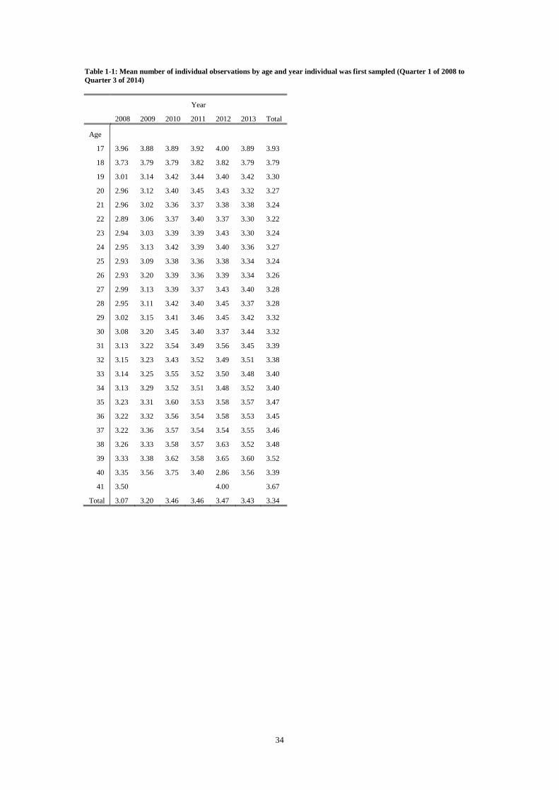
Table 1-1 below shows that attrition is likely correlated with the age of the respondents

because the average number of observations for an individual is increasing with age in these

samples (note that those respondents aged 17 (or 41) in this table (Table 1-1) are workers that

were 19 (or 39) at some point while they are part of the sample). We propose a simple

solution to address this non-random attrition when we estimate state dependence in

unemployment. This involves setting the missing labour market states for the individuals that

enter the dwelling only after it is first sampled to ‘missing’ (for those periods the dwelling is

in the sample frame). We set the missing values for age to the age of the worker in the period

when the worker enters or re-enters the dwelling. In order to avoid double counting the

individuals that move we will also exclude any respondents from the subsequent analysis who

move out of the dwelling and do not return. The intuition here is that, by expanding datum in

the sample to reflect a missing state for the quarters prior to entering a dwelling for those

33

individuals that enter the dwelling only after it is first sampled, these individuals have a ‘twin’

that leaves another dwelling before it is sampled for the fourth and final time.

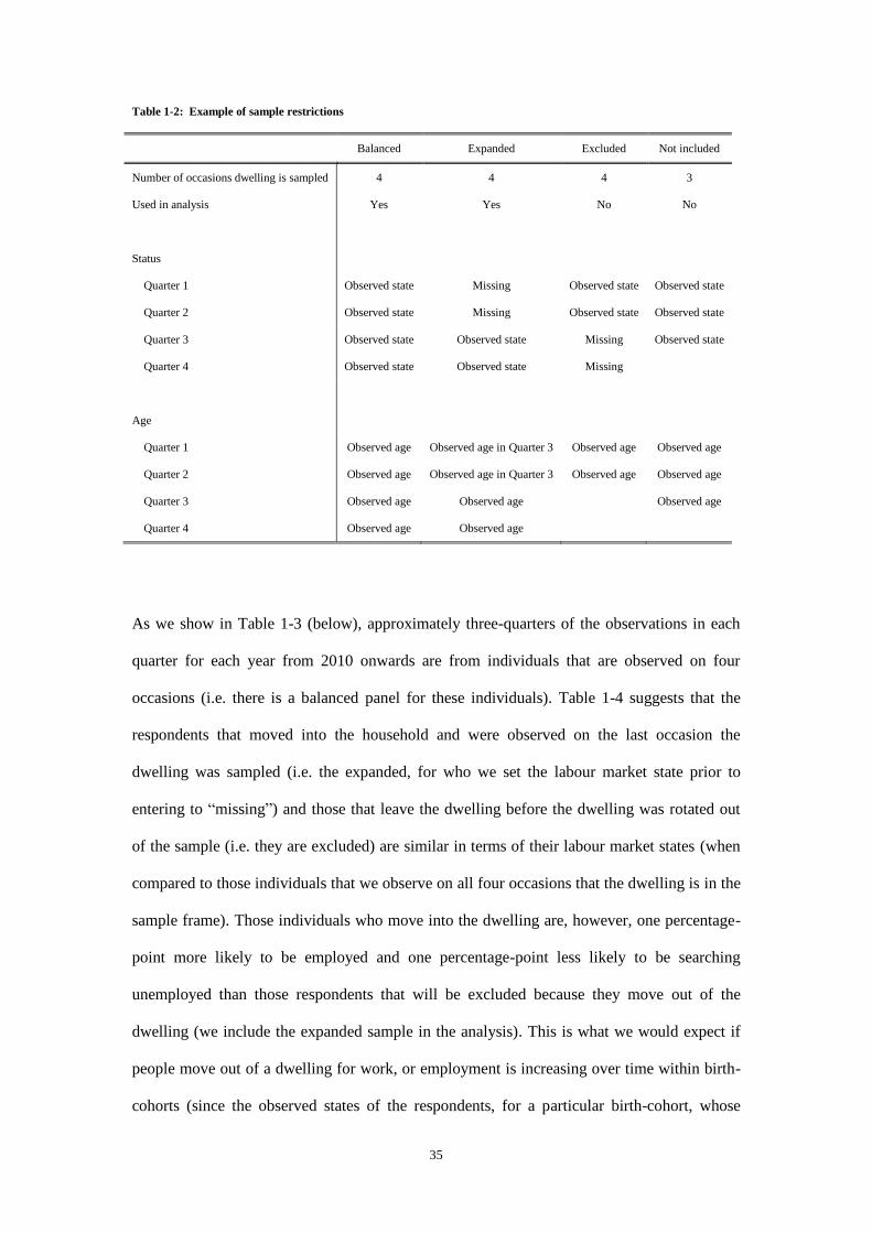
We do not include the observations from those dwellings that were surveyed on fewer than

four occasions. This restriction extends to approximately 20% of the individuals in the

original sample of cross-sections. While the majority of these observations are from dwellings

that were randomly phased out by Stats SA, they also include dwellings (approximately 10%

of the dwellings that were surveyed in any given quarter) where nobody in the dwelling was

willing to respond to the survey (perhaps because all the respondents that had been living in

the dwelling had moved out). We will assume that this does not influence the generalizability

of the results to a large proportion of the population. Table 1-2 (below) illustrates the

restrictions on the sample that will be used in the subsequent sections of this chapter.

34

Table 1-1: Mean number of individual observations by age and year individual was first sampled (Quarter 1 of 2008 to

Quarter 3 of 2014)

Year

2008 2009 2010 2011 2012 2013 Total

Age

17 3.96 3.88 3.89 3.92 4.00 3.89 3.93

18 3.73 3.79 3.79 3.82 3.82 3.79 3.79

19 3.01 3.14 3.42 3.44 3.40 3.42 3.30

20 2.96 3.12 3.40 3.45 3.43 3.32 3.27

21 2.96 3.02 3.36 3.37 3.38 3.38 3.24

22 2.89 3.06 3.37 3.40 3.37 3.30 3.22

23 2.94 3.03 3.39 3.39 3.43 3.30 3.24

24 2.95 3.13 3.42 3.39 3.40 3.36 3.27

25 2.93 3.09 3.38 3.36 3.38 3.34 3.24

26 2.93 3.20 3.39 3.36 3.39 3.34 3.26

27 2.99 3.13 3.39 3.37 3.43 3.40 3.28

28 2.95 3.11 3.42 3.40 3.45 3.37 3.28

29 3.02 3.15 3.41 3.46 3.45 3.42 3.32

30 3.08 3.20 3.45 3.40 3.37 3.44 3.32

31 3.13 3.22 3.54 3.49 3.56 3.45 3.39

32 3.15 3.23 3.43 3.52 3.49 3.51 3.38

33 3.14 3.25 3.55 3.52 3.50 3.48 3.40

34 3.13 3.29 3.52 3.51 3.48 3.52 3.40

35 3.23 3.31 3.60 3.53 3.58 3.57 3.47

36 3.22 3.32 3.56 3.54 3.58 3.53 3.45

37 3.22 3.36 3.57 3.54 3.54 3.55 3.46

38 3.26 3.33 3.58 3.57 3.63 3.52 3.48

39 3.33 3.38 3.62 3.58 3.65 3.60 3.52

40 3.35 3.56 3.75 3.40 2.86 3.56 3.39

41 3.50

4.00

3.67

Total 3.07 3.20 3.46 3.46 3.47 3.43 3.34

35

Table 1-2: Example of sample restrictions

Balanced Expanded Excluded Not included

Number of occasions dwelling is sampled 4 4 4 3

Used in analysis Yes Yes No No

Status

Quarter 1 Observed state Missing Observed state Observed state

Quarter 2 Observed state Missing Observed state Observed state

Quarter 3 Observed state Observed state Missing Observed state

Quarter 4 Observed state Observed state Missing

Age

Quarter 1 Observed age Observed age in Quarter 3 Observed age Observed age

Quarter 2 Observed age Observed age in Quarter 3 Observed age Observed age

Quarter 3 Observed age Observed age

Observed age

Quarter 4 Observed age Observed age

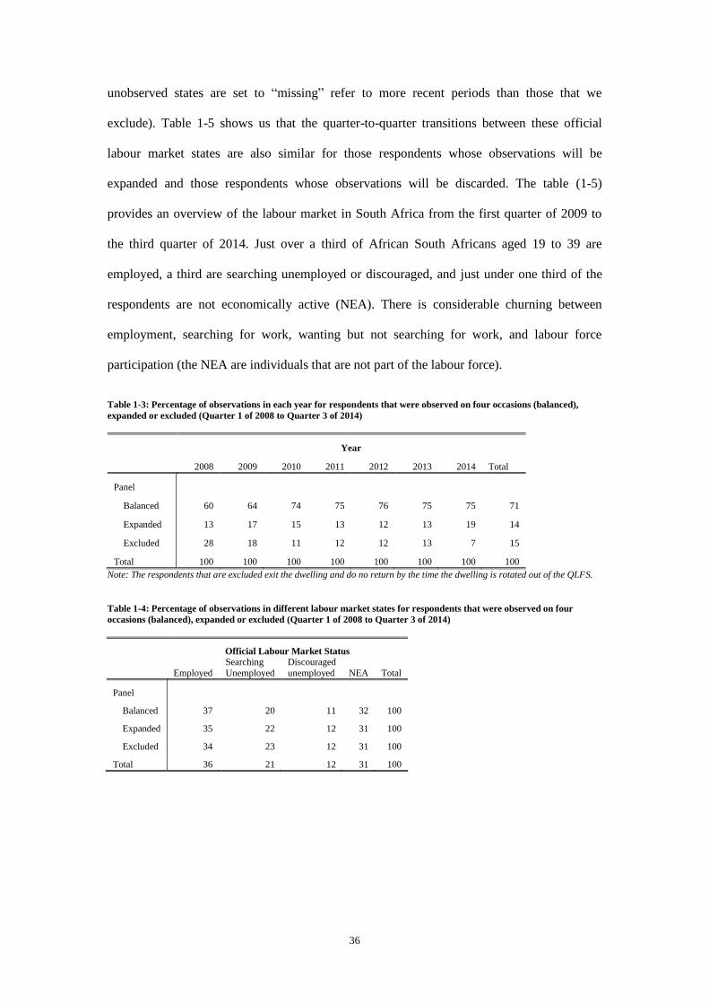
As we show in Table 1-3 (below), approximately three-quarters of the observations in each

quarter for each year from 2010 onwards are from individuals that are observed on four

occasions (i.e. there is a balanced panel for these individuals). Table 1-4 suggests that the

respondents that moved into the household and were observed on the last occasion the

dwelling was sampled (i.e. the expanded, for who we set the labour market state prior to

entering to “missing”) and those that leave the dwelling before the dwelling was rotated out

of the sample (i.e. they are excluded) are similar in terms of their labour market states (when

compared to those individuals that we observe on all four occasions that the dwelling is in the

sample frame). Those individuals who move into the dwelling are, however, one percentage-

point more likely to be employed and one percentage-point less likely to be searching

unemployed than those respondents that will be excluded because they move out of the

dwelling (we include the expanded sample in the analysis). This is what we would expect if

people move out of a dwelling for work, or employment is increasing over time within birth-

cohorts (since the observed states of the respondents, for a particular birth-cohort, whose

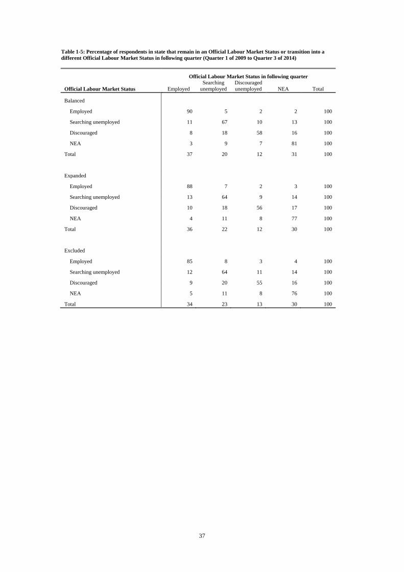
36

unobserved states are set to “missing” refer to more recent periods than those that we

exclude). Table 1-5 shows us that the quarter-to-quarter transitions between these official

labour market states are also similar for those respondents whose observations will be

expanded and those respondents whose observations will be discarded. The table (1-5)

provides an overview of the labour market in South Africa from the first quarter of 2009 to

the third quarter of 2014. Just over a third of African South Africans aged 19 to 39 are

employed, a third are searching unemployed or discouraged, and just under one third of the

respondents are not economically active (NEA). There is considerable churning between

employment, searching for work, wanting but not searching for work, and labour force

participation (the NEA are individuals that are not part of the labour force).

Table 1-3: Percentage of observations in each year for respondents that were observed on four occasions (balanced),

expanded or excluded (Quarter 1 of 2008 to Quarter 3 of 2014)

Year

2008 2009 2010 2011 2012 2013 2014 Total

Panel

Balanced 60 64 74 75 76 75 75 71

Expanded 13 17 15 13 12 13 19 14

Excluded 28 18 11 12 12 13 7 15

Total 100 100 100 100 100 100 100 100

Note: The respondents that are excluded exit the dwelling and do no return by the time the dwelling is rotated out of the QLFS.

Table 1-4: Percentage of observations in different labour market states for respondents that were observed on four

occasions (balanced), expanded or excluded (Quarter 1 of 2008 to Quarter 3 of 2014)

Official Labour Market Status

Employed

Searching

Unemployed

Discouraged

unemployed NEA Total

Panel

Balanced 37 20 11 32 100

Expanded 35 22 12 31 100

Excluded 34 23 12 31 100

Total 36 21 12 31 100

37

Table 1-5: Percentage of respondents in state that remain in an Official Labour Market Status or transition into a

different Official Labour Market Status in following quarter (Quarter 1 of 2009 to Quarter 3 of 2014)

Official Labour Market Status in following quarter

Official Labour Market Status Employed

Searching

unemployed

Discouraged

unemployed NEA Total

Balanced

Employed 90 5 2 2 100

Searching unemployed 11 67 10 13 100

Discouraged 8 18 58 16 100

NEA 3 9 7 81 100

Total 37 20 12 31 100

Expanded

Employed 88 7 2 3 100

Searching unemployed 13 64 9 14 100

Discouraged 10 18 56 17 100

NEA 4 11 8 77 100

Total 36 22 12 30 100

Excluded

Employed 85 8 3 4 100

Searching unemployed 12 64 11 14 100

Discouraged 9 20 55 16 100

NEA 5 11 8 76 100

Total 34 23 13 30 100

38

Descriptions of the data

In this section (and the rest of this chapter) we will distinguish between six labour market

states: formal employed, informal (and self) employed, short term unemployed, long term

unemployed, not economically active (NEA), and missing (where missing is captured as a

state and does not imply that the observations are discarded). We use the official definition of

formal wage-employment that we outlined in the previous section. The informally employed

are the respondents that are not formally employed including those that are defined as ‘other’.

The group ‘other’ account for only 1.4% of all the observations in the sample, and the

majority of the self-employed are own-account workers. This is why we will refer to this

group as the informal employed even though a small number of observations in this group

refer to individuals that own registered firms. The primary distinction between the two

employment states for the purposes of our analysis is that those workers that are formally

employed are protected by labour law while those individuals that are ‘informally’ (in this

context) employed are not. The short term unemployed include both the searching

unemployed who have been searching for work for less than one year and discouraged job

seekers that have been employed in the past year. The long term unemployed are the

searching unemployed or discouraged job seekers that have been searching for work for more

than one year, last had a job more than a year ago, or have never had a job.

We will not use the observations for respondents that were first sampled in 2008 (i.e. those

dwellings that enter the sample in the first, second, third or fourth quarter of 2008) for two

reasons: Attrition was particularly severe in 2008; and the variable distinguishing between

formal and informal employment was not included in the official release of the QLFS cross-

sections for 2008. As mentioned we also exclude those observations for individuals that move

out of the dwelling and do not return before the dwelling is rotated out of the sample to avoid

“double-counting” the transitions of workers that move dwellings (since we now include data

for workers in the periods the dwellings they moved into were in the sample by setting their

labour market state to “missing”).

39

There are an overwhelming number of state-period-age combinations. Consequently, we

alternate between presenting aggregates (for 2009 to 2014) that provide the reader with an

overview of the relationship between these states (and age), and figures that provide us with a

dynamic view of these outcomes over the 23 quarters in these six years (at the time of writing

we did not have the data for Quarter 4 of 2014) at different ages (and for different birth-

cohorts). We will present the figures (and conduct any analysis) separately for males and

females because there are differences in the percentage of males and females that are in each

of these states at different ages and because it is likely that there may be systematic

differences in the transactions costs associated with finding and staying in employment

between gender. Notably females are more likely to have to look after children and many

females with children are eligible for the Child Support Grant (CSG). From the perspective of

firms there may also be more uncertainty regarding the returns associated with training

female workers if these females fall pregnant, and females may be more likely than their male

counterparts to exit employment for a period when they have children.

Table 1-6 and Table 1-7 present the percentage of respondents in each state by age (and age

group) for African males and females respectively. It is interesting to note that the proportions

of African South Africans that are unemployed are more similar for workers in their twenties

than they are for those in their thirties. The majority of the unemployed aged 20 to 29 are

what we define as long term unemployed. Workers aged 20-24 are far less likely to be

employed than their older counterparts. There is nevertheless considerable heterogeneity

within the 20-24 age-group. For example more than half of the respondents aged 20 were not

economically active. In contrast more than three quarters of those aged 24 are in the labour

force.

In Figure 1-1 and Figure 1-2 we provide an overview of the percentage of African Males and

Females that are in one of the six states at ages 19 through to 39 (from the first quarter of

2009 to the third quarter of 2014). We see that the missing-state observations make up a large

fraction of the observations in 2009. However from 2010 onwards the percentage of missing

40

observations is similar between years. The figures also highlight several important features of

the labour market from 2009 to 2014. First, labour force participation rates are very low

among workers aged 19; and while there is a large increase from age 20 labour force

participation is lower among Africans aged 20 to 24 than it is for those that are 25 or older.

Second, unemployment is persistent for both males and females and high even among those

workers that are not officially regarded as youth in South Africa. Third, formal wage-

employment is more prevalent than other forms of employment. It appears that formal

employment is increasing and the other forms of employment have been decreasing among

successive female birth-cohorts (we can see the relationship between these states and birth-

cohorts by following the diagonals in the figures).

41

Table 1-6: Percentage of male respondents in each state by age (Quarter 1 of 2009 to Quarter 3 of 2014).

State

Missing NEA

Short term

Unemployed

Long term

Unemployed

Formal

Employed

Informal

Employed Total

Age

17 0 100 0 0 0 0 100

18 4 84 3 6 0 2 100

19 12 70 5 9 1 2 100

20 14 53 8 16 3 5 100

21 13 42 9 22 7 7 100

22 15 30 10 25 10 9 100

23 15 23 11 26 15 11 100

24 14 16 12 26 19 13 100

25 15 13 11 25 22 14 100

26 15 12 10 25 24 15 100

27 14 9 10 22 27 17 100

28 13 10 10 20 28 19 100

29 15 8 9 20 30 18 100

30 13 9 10 21 30 19 100

31 14 9 9 18 32 19 100

32 12 8 8 17 35 20 100

33 13 8 8 15 36 20 100

34 11 8 8 15 38 20 100

35 11 10 8 14 36 21 100

36 12 9 7 14 37 20 100

37 11 11 8 14 35 20 100

38 11 10 7 14 37 20 100

39 9 11 7 14 38 21 100

40 4 12 7 14 42 22 100

41 0 0 13 26 39 22 100

Total 13 23 9 19 22 14 100

Age group

20 - 24 14 34 10 23 10 9 100

25 - 29 14 11 10 23 26 16 100

30 - 34 13 8 9 17 34 20 100

35 - 39 11 10 7 14 36 20 100

Total 13 18 9 20 24 15 100

Labour force participation is increasing until approximately age 25 after which it remains fairly stable. Both short term and long

term unemployment are increasing until age 24 after which they decrease. The percentage of each age-cohort in formal and

informal employment is increasing with age. There is also considerable heterogeneity within the broadly defined age-groups.

42

Table 1-7: Percentage of female respondents in each state by age (Quarter 1 of 2009 to Quarter 3 of 2014).

State

Missing NEA

Short term

Unemployed

Long term

Unemployed

Formal

Employed

Informal

Employed Total

Age

17 2 90 0 8 0 0 100

18 4 84 3 7 0 1 100

19 13 69 5 10 2 1 100

20 15 56 7 17 3 3 100

21 14 46 8 23 5 4 100

22 14 38 8 27 7 5 100

23 15 32 9 28 10 6 100

24 14 28 9 29 12 7 100

25 14 25 9 28 15 8 100

26 13 24 8 29 16 10 100

27 14 22 8 27 18 10 100

28 12 22 8 26 20 11 100

29 12 24 7 25 21 11 100

30 12 23 8 25 21 11 100

31 12 22 7 25 22 13 100

32 11 21 7 24 23 13 100

33 10 22 6 22 23 16 100

34 10 22 6 21 24 16 100

35 10 22 6 22 24 16 100

36 9 23 6 20 24 18 100

37 10 22 6 19 25 18 100

38 9 21 6 19 27 18 100

39 9 21 6 18 26 20 100

40 2 24 5 19 29 20 100

41 0 21 5 26 37 11 100

Total 12 32 7 23 16 10 100

Age group

20 - 24 14 40 8 25 7 5 100

25 - 29 13 23 8 27 18 10 100

30 - 34 11 22 7 23 23 14 100

35 - 39 9 22 6 20 25 18 100

Total 12 28 7 24 17 11 100

Labour force participation is increasing until approximately age 25 after which it remains fairly stable. Both short term and long

term unemployment are increasing until age 24 after which they decrease. The percentage of each age-cohort in formal and

informal employment is increasing with age. There is also considerable heterogeneity within the broadly defined age-groups.

43

Figure 1-1: Percentage of African Male age-cohort in state (Quarter 1 of 2009 to Quarter 3 of 2014)

Figure 1-2: Percentage of African Female age-cohort in state (Quarter 1 of 2009 to Quarter 3 of 2014)

44

We now turn our attention to the transitions between these states. Table 1-8 suggests that

there is considerable churning between non-economic activity and unemployment,

particularly for females. This highlights one of the problems with both the measure of

unemployment and the duration of unemployment in our data. We see that a share of the

respondents that are not economically active in any given quarter transition into long term

unemployment. This is why we do not use the questions about how long the respondent has

been searching for work (or how long it has been since the respondent last worked) to fill in

the states for the respondents where these states are missing. The long term unemployed also

include discouraged job-seekers who have never had (what they regarded as) a job. We also

note that some of the long term unemployed transition into short term unemployment. This

may be due to measurement error, although it may also reflect those situations where a long

term unemployed respondent finds and then leaves/loses a job between quarters. The

transitions from long term and short term unemployment nevertheless confirm our priors: The

short term unemployed are less likely to stay unemployed than the long term unemployed,

and the short term unemployed are more likely to transition into formal and informal

employment than the long term unemployed. Interestingly, those respondents who transition

out of unemployment are more likely to enter informal employment than formal employment

even though, as we showed earlier in this section, formal employment is more prevalent than

informal employment among the respondents in our sample. Another important feature of the

labour market from 2009 to 2014 for the respondents in our sample is that a large proportion

of workers exit employment into unemployment. The informally employed are also more

likely to transition into unemployment than the respondents in formal employment.

It is notable that proportionally more of the informally employed transition into formal

employment than the short term unemployed (conversely, a smaller percentage of the formal

employed transition into informal employment). The transitions we have outlined are

aggregates for all individuals aged 19 to 39 (in at least one of the periods they are observed)

in the sample. In Table 1-9 and Table 1-10 we present the percentage of respondents in each

45

of the six states that transition into unemployment (or in the case of those that are long term

and short term unemployed remain unemployed) from one quarter to the next, by age. It

seems that unemployment is more persistent among younger age-cohorts. However it also

appears that younger employed African South Africans are more likely than their older peers

to transition into unemployment from employment. The figures suggest though that the

persistence in unemployment contributes more to unemployment than these transitions from

employment. More than 85% of the long term unemployed in any given quarter are

unemployed (i.e. they want work) in the following quarter, and this figure is higher among

those in the age group 20 to 24 than it is in older age-groups. Further, as we show in Figure 1-

3 and Figure 1-4, the persistence in unemployment from short term unemployment is also

more distinct among the youngest workers. This implies that unemployment may be related to

the characteristics of the unemployed, such as their age (but also work experience etc.). The

only (immediately) visible change in the relationship between age and these labour market

states across years is that, from 2013 onwards, a larger proportion of males younger than 25

left informal employment and transitioned into unemployment than in the preceding surveys9.

9 There is also a spot in 2014 for those males that were around the eligibility threshold for the Youth Employment

Tax Incentive (ETI) that we outlined in the introduction to this thesis (only workers younger than 30 are eligible,

from the fourth quarter of 2013). While Ranchhod and Finn (2014) find that the ETI had no effect on employment

in the first two quarters of 2014, this finding is based on a Difference in Difference (DID) estimate that assumes

the ETI had no effect on employment in the fourth quarter of 2013. However, firms were allowed to make

retroactive claims for employees from October 2013. Our analysis of the effect of the ETI using the same data that

we do in this chapter suggests that ETI may have, not surprisingly, increased formal employment and decreased

informal employment among young African males that are eligible for the subsidy. Our identification strategy, like

in Ranchhod and Finn (2014), assumes that those around the threshold have parallel trends. The results we present

in this paper suggest, though, that this may be a tenuous assumption. Furthermore we are concerned that the

eligible workers are merely more likely to be aware that they work for firms that are, for example, registered for

VAT and Income Tax. We therefore present these and the other impacts of the ETI on labour market outcomes in a

separate paper.

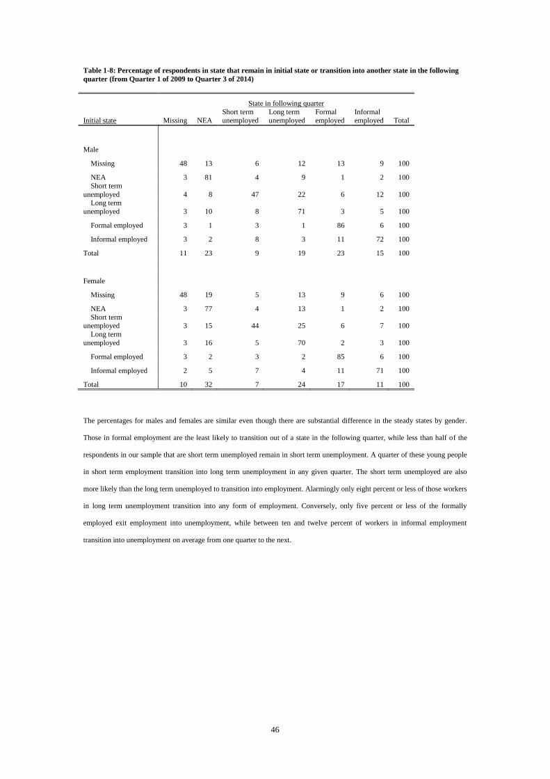
46

Table 1-8: Percentage of respondents in state that remain in initial state or transition into another state in the following

quarter (from Quarter 1 of 2009 to Quarter 3 of 2014)

State in following quarter

Initial state Missing NEA

Short term

unemployed

Long term

unemployed

Formal

employed

Informal

employed Total

Male

Missing 48 13 6 12 13 9 100

NEA 3 81 4 9 1 2 100

Short term

unemployed 4 8 47 22 6 12 100 Long term

unemployed 3 10 8 71 3 5 100

Formal employed 3 1 3 1 86 6 100

Informal employed 3 2 8 3 11 72 100

Total 11 23 9 19 23 15 100

Female

Missing 48 19 5 13 9 6 100

NEA 3 77 4 13 1 2 100

Short term unemployed 3 15 44 25 6 7 100

Long term

unemployed 3 16 5 70 2 3 100

Formal employed 3 2 3 2 85 6 100

Informal employed 2 5 7 4 11 71 100

Total 10 32 7 24 17 11 100

The percentages for males and females are similar even though there are substantial difference in the steady states by gender.

Those in formal employment are the least likely to transition out of a state in the following quarter, while less than half of the

respondents in our sample that are short term unemployed remain in short term unemployment. A quarter of these young people

in short term employment transition into long term unemployment in any given quarter. The short term unemployed are also

more likely than the long term unemployed to transition into employment. Alarmingly only eight percent or less of those workers

in long term unemployment transition into any form of employment. Conversely, only five percent or less of the formally

employed exit employment into unemployment, while between ten and twelve percent of workers in informal employment

transition into unemployment on average from one quarter to the next.

47

Table 1-9: Percentage of African males in state that are unemployed in the following quarter (from Quarter 1 of 2009 to

Quarter 3 of 2014)

Initial state

Missing NEA

Short term

Unemployed

Long term

Unemployed

Formal

Employed

Informal

Employed Total

Age

17 0 8 0 0 0 0 8

18 12 8 91 91 19 19 16

19 12 13 86 92 10 18 23

20 18 17 88 92 13 19 34

21 22 20 81 91 11 20 40

22 22 23 81 91 10 18 43

23 25 24 81 90 8 16 43

24 26 28 80 88 8 17 43

25 23 28 80 89 6 17 40

26 22 31 76 89 6 14 39

27 21 28 79 88 5 13 36

28 19 27 73 87 5 12 33

29 19 25 73 88 5 10 31

30 20 25 71 87 5 11 33

31 17 23 74 86 4 12 29

32 16 23 73 87 4 10 27

33 18 23 76 87 3 8 25

34 16 18 74 88 3 8 24

35 15 22 74 88 3 10 25

36 19 22 70 86 3 9 24

37 14 15 71 89 3 9 25

38 13 19 72 88 3 8 24

39 15 16 67 89 2 7 23

40 28 20 76 88 2 7 23

41 0 0 0 100 0 50 38

Total 19 18 78 89 5 12 32

Age group

20 - 24 22 21 82 90 9 18 40

25 - 29 21 28 77 88 5 13 36

30 - 34 17 22 73 87 4 10 28

35 - 39 15 19 71 88 3 9 24

Total 20 22 77 89 5 12 33

There are differences in the proportion of missing-state respondents that are unemployed in the following quarter. Initially these

percentages increase with age until 25 after which they start to decline. The proportion of non-economically active respondents

that transition into unemployment is also initially increasing with age until age 26 after which these percentages start to decline.

In contrast the percentage of respondents in both forms of unemployment and both forms of employment that are unemployed in

the following quarter is decreasing with age.

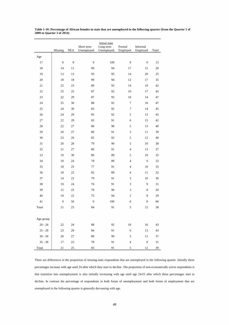
48

Table 1-10: Percentage of African females in state that are unemployed in the following quarter (from the Quarter 1 of

2009 to Quarter 3 of 2014)

Initial state

Missing NEA

Short term

Unemployed

Long term

Unemployed

Formal

Employed

Informal

Employed Total

Age

17 0 8 0 100 0 0 15

18 14 11 90 94 17 15 20

19 13 13 93 95 14 20 25

20 18 18 90 94 12 17 35

21 22 23 89 92 14 19 42

22 25 25 87 92 10 17 45

23 22 29 87 93 10 14 47

24 25 30 88 92 7 16 47

25 24 30 83 92 7 14 45

26 24 29 85 92 5 13 45

27 22 29 83 91 6 15 42

28 22 27 86 90 5 13 40

29 20 27 80 91 5 11 39

30 23 26 82 92 5 12 40

31 20 28 79 90 5 10 38

32 21 27 80 91 4 13 37

33 19 30 80 89 5 10 35

34 19 24 78 89 4 9 33

35 18 25 77 91 4 10 35

36 18 22 82 89 4 11 32

37 14 22 79 91 3 10 30

38 19 24 76 91 3 9 31

39 15 25 78 90 3 8 29

40 19 22 75 94 2 8 29

41 0 50 0 100 0 0 60

Total 21 23 84 91 5 12 38

Age group

20 - 24 22 24 88 92 10 16 43

25 - 29 23 29 84 91 6 13 43

30 - 34 20 27 80 90 5 11 37

35 - 39 17 23 78 91 4 9 31

Total 21 25 83 91 5 12 39

There are differences in the proportion of missing-state respondents that are unemployed in the following quarter. Initially these

percentages increase with age until 24 after which they start to decline. The proportion of non-economically active respondents is

that transition into unemployment is also initially increasing with age until age 24/25 after which these percentages start to

decline. In contrast the percentage of respondents in both forms of unemployment and both forms of employment that are

unemployed in the following quarter is generally decreasing with age.

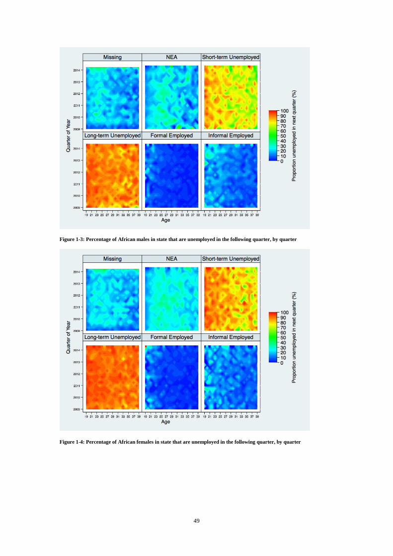
49

Figure 1-3: Percentage of African males in state that are unemployed in the following quarter, by quarter

Figure 1-4: Percentage of African females in state that are unemployed in the following quarter, by quarter

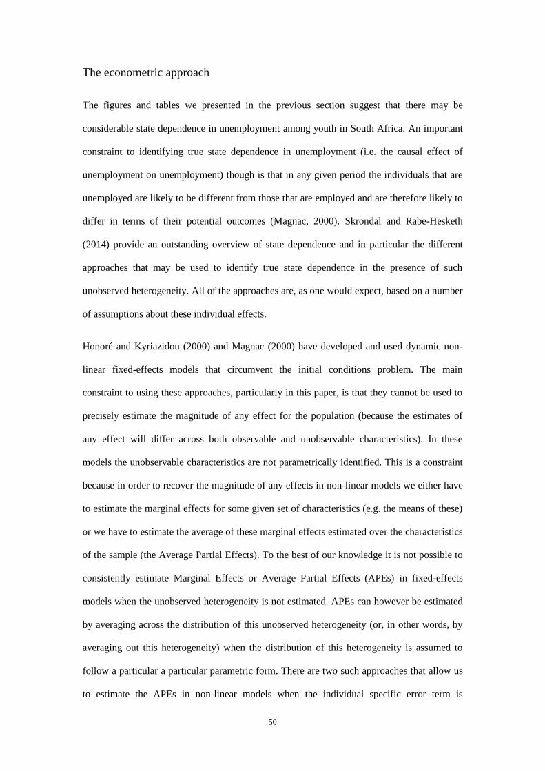
50

The econometric approach

The figures and tables we presented in the previous section suggest that there may be

considerable state dependence in unemployment among youth in South Africa. An important

constraint to identifying true state dependence in unemployment (i.e. the causal effect of

unemployment on unemployment) though is that in any given period the individuals that are

unemployed are likely to be different from those that are employed and are therefore likely to

differ in terms of their potential outcomes (Magnac, 2000). Skrondal and Rabe-Hesketh

(2014) provide an outstanding overview of state dependence and in particular the different

approaches that may be used to identify true state dependence in the presence of such

unobserved heterogeneity. All of the approaches are, as one would expect, based on a number

of assumptions about these individual effects.

Honoré and Kyriazidou (2000) and Magnac (2000) have developed and used dynamic non-

linear fixed-effects models that circumvent the initial conditions problem. The main

constraint to using these approaches, particularly in this paper, is that they cannot be used to

precisely estimate the magnitude of any effect for the population (because the estimates of

any effect will differ across both observable and unobservable characteristics). In these

models the unobservable characteristics are not parametrically identified. This is a constraint

because in order to recover the magnitude of any effects in non-linear models we either have

to estimate the marginal effects for some given set of characteristics (e.g. the means of these)

or we have to estimate the average of these marginal effects estimated over the characteristics

of the sample (the Average Partial Effects). To the best of our knowledge it is not possible to

consistently estimate Marginal Effects or Average Partial Effects (APEs) in fixed-effects

models when the unobserved heterogeneity is not estimated. APEs can however be estimated

by averaging across the distribution of this unobserved heterogeneity (or, in other words, by

averaging out this heterogeneity) when the distribution of this heterogeneity is assumed to

follow a particular a particular parametric form. There are two such approaches that allow us

to estimate the APEs in non-linear models when the individual specific error term is

51

correlated with the initial state. Heckman (1981) explicitly models the unobserved

heterogeneity associated with the initial condition, while Wooldridge’s (2005) solution

approximates the unobserved characteristics by modeling any individual dynamics

conditional on the initial state.

We use Wooldridge’s (2005) simple solution to address this initial conditions problem

because it provides us with what (we believe) is likely to be the best possible approximation

(given the data, the assumptions we have to make, and our objective). Skrondal and Rabe-

Hesketh (2013) point out that Heckman’s (1981) model for the initial response should also

include pre-sample time-varying covariates. There are no pre-sample time-varying covariates

that we could reasonably argue are strictly exogenous in the data that is available to this

chapter. Further while Akay (2012) finds that Wooldridge’s (2005) estimator performs poorly

(when compared to Heckman’s approach) for panels with fewer than five individual

observations, Skrondal and Rabe-Hesketh (2013) find that it is only biased when the

unobserved heterogeneity associated with any potentially endogenous characteristics is

approximated using the averages over all periods for these covariates. Skrondal and Rabe-

Hesketh (2013) propose using either Wooldridge’s (2005) original specification where the

measure for any given period is included in the estimation for each time period or, when the

average is used, to also include the initial value in each period.

The specification we use is adapted from another paper which uses the same approach to

explore labour market outcomes. Stewart (2007) specifies different dummies for

combinations of unemployment and low-wage employment (in t-2 and t-1 i.e. two and one

periods prior to the current period) even though the dependent variable is binary. We use the

six lagged labour market states that we outlined in the previous section: formal employed,

52

informal employed (which includes a small number of registered firm owners), short term

unemployed, long term unemployed, not economically active, and “missing”10.

The binary dependent variable for the unemployed is defined if the individual is in either

short term or long term unemployment, or when the respondent is missing in this period but

enters the dwelling as one of these two (i.e. long term and short term) forms of

unemployment. While Stewart’s (2007) estimates extend only to those individuals that are in

the labour force, we include transitions into the labour market in our model because we are

focusing on younger workers. Further we do not exclude those respondents that do not

transition into the labour force in any of the four periods they are observed. We are concerned

that this will compromise the assumptions (which we will outline shortly) we have to make

about the distribution of the individual heterogeneity in each of these states because this

would in effect truncate the distribution of this heterogeneity. We also specify the initial and

lagged states of those observations that are missing as a separate state to limit any bias from

non-random attrition. Wooldridge (2005:44) points out that if the data is not missing

completely at random (MCAR) the density obtained using this simple solution for

specifications that include a lagged dependent variable has the advantage that it would not

only be conditional on the exogenous explanatory variables, but also depend on the initial

state in “an arbitrary way.”11

10 We considered distinguishing between short-term and long-term employment. However, we do not know how

long the respondents with jobs have been in employment because we do not know what they were doing prior to

their current job. They may have been employed in a different job. In contrast we know how long the unemployed

have been unemployed for (or that they have never had a job).

11 Skrondal and Rabe-Hesketh (2014: 224) point out that that, while the “[i]solated observations (preceded and

succeeded by missing data) cannot be used… it is possible to utilize several sequences of non-missing data for a

subject (e.g. 11.11). In this case “the ‘initial’ values of the response and time-varying covariates change between

sequences (for example, for 11.11, the initial response is y0j for the first sequence and y3j for the second

sequence). It is possible to let the parameters of the auxiliary model differ depending on which occasion is the

initial occasion. Another possibility is to analyse only those contiguous sequences of non-missing data that start at

53

We estimate the effects of being in one of the six different labour market states in the

previous quarter (which we denote as t-1) on unemployment in the quarter (t) at different

levels of age (i.e. we estimate each specification separately for workers at this age) by

estimating the following Random Effects Probit specification (where the notation is also

adapted from Wooldridge, 2005):

𝑃(𝑦i,t = 1| �⃗�i,t-1, �⃗�i,t-2, … , �⃗�i,0, 𝑝it, 𝑐i) = 𝛷(β[�⃗�i,t-1, 𝑝it] + 𝑐i + 𝑢it) (1)

In this specification 𝑦i,t = 1 if unemployed and zero otherwise, �⃗�i,t-1 is the vector of six lagged

states (we use one of these six – long term unemployment – as the reference state when we

estimate the specification; the other states are missing, not economically active (NEA), short

term unemployment, formal employment and informal employment), 𝑝it is the time period,

and 𝑐i is the unobserved individual-specific effect, 𝛷 is the cumulative normal distribution,

and the unobserved fixed-effect is approximated as 𝑐i = α0 + αi[�⃗�i0 , pi0] + ai where 𝑎i| �⃗�i0, 𝑝i0

~ 𝑁(𝛼0 + 𝛼1[�⃗�i0 , 𝑝i0], 𝜎a2). We also use long term unemployed in the initial state vector �⃗�i0 as

the reference category. 𝜎a2 is the variance of 𝑎i| �⃗�i0, 𝑝i0, and 𝑢it is the idiosyncratic error term

where 𝑢it| �⃗�i,t-1 , 𝑝it, 𝑐i ~ 𝑁(0,1).

The binary dependent variable model is, we believe, sufficient for the purposes of this chapter

because we are interested in state dependence in unemployment. 12 In our case this is

measured as the difference in the conditional probability of exiting employment into

unemployment and the conditional probability of staying unemployed from one quarter to the

next. This approach does not consider the effect on unemployment of those individuals that

leave the labour force from employment or unemployment (perhaps because of an illness). 𝑝i0

is included because we will pool the data for particular years (to increase the precision of the

occasion 0, i.e. to discard subjects with patterns such as (..11). In these somewhat ad hoc approaches, the missing

values… are implicitly imputed… and the responses are assumed to be missing at random.”

12 The multinomial alternatives are also computationally demanding (and finding the maximum likelihood is a

more precarious endeavor).

54

point estimates for each year). As mentioned we have data for individuals for at most four

quarters and we will we refer to this as a “panel-section”. In this chapter we will estimate the

specification for five different pools from the year that the dwelling was first sampled. For

example, the 2013/2014 pool refers to those panel-sections that were initially sampled in the

first quarter of 2013 (and were rotated out in the fourth quarter of 2013) and all subsequent

sections until (including) those sections that were initially sampled in the fourth quarter of

2013 (and were rotated out in the third quarter of 2014). We will compare these estimates to

the estimates for those respondents that were initially sampled in the first quarter of 2009 (and

were rotated out in the fourth quarter of 2009) and ending with those sections that were

initially sampled in the fourth quarter of 2009 (and were rotated out in the third quarter of

2010); those respondents that were initially sampled in the first quarter of 2010 (and were

rotated out in the fourth quarter of 2010) and end with those sections that were initially

sampled in the fourth quarter of 2010 (and were rotated out in the third quarter of 2011); etc.

𝑝i0 serves two purposes. First the initial period the respondent was sampled in controls for

some of the variation between panel-sections that can be attributed to the rotation scheme and

implementation of the survey. Second, since we estimate the specification for the respondents

at a particular age, it may capture any ‘residual’ (i.e. after we condition on the initial state)

birth-cohort effects associated with the different birth-cohorts in these age-samples13 (the

approach we use does not separately identify any cohort effects because these effects are part

of the model for the initial conditions, although it is unlikely that there will be substantial

cohort effects over the course of one year). Naturally we still expect our measure of state

dependence for any given year to be related to the level of aggregate demand for labour and

13 Further we define a particular age-sample, say 21, if the respondent indicated that they were 21 at any period

that they are observed. These age-samples are, consequently, not mutually exclusive. However, we do this because

there appears to be some measurement error associated with this variable (particular among proxy-responses). We

ensure that the APEs are mutually exclusive by, as will describe in more detail shortly, only making predictions

onto those observations where the respondent’s age corresponds to the particular age-sample.

55

the competition for jobs during this quarter, among others (including anything else that has an

effect on the distribution of transaction costs etc.)14.

In this chapter we do not estimate the specification for different subgroups defined by

education because, while state dependence in unemployment may vary across these groups,

education levels have been increasing among consecutive birth-cohorts and we have no

reason to believe that in South Africa education is a better predictor of most of these workers’

skills than the initial labour market states that we use in our model (see Mariotti and

Meinecke, 2014). Furthermore we do not include education or any of the other time-varying

or time-invariant individual-level covariates that are available in the dataset (the only

candidates are province, geography, and marital status) because there is very little individual-

level variation in education and marital status (and province and geography are fixed).

Wooldridge (2005) points out that we cannot separately identify the partial effect of time-

constant variables from their partial correlation with the unobserved heterogeneity and they

should only be included to increase the precision of the estimator. When we include these

variables (education – which we set to the first level that is observed for those missing-state

respondents that enter the dwelling, the location of the dwelling, and the corresponding

specification for the unobserved heterogeneity for individuals who accumulate higher levels

of education while they are in the sample frame) the point estimates are nearly identical to

those that we will present in the next section, and there are no gains in efficiency that would

alter the conclusions we draw in the following section. We therefore implicitly condition on

work experience and education etc. through the initial state. While this may seem

disconcerting to some readers it should be noted that, even when we condition on individual

fixed-effects, including education and work experience violates the assumptions of the

14 For example, we anticipate (but do not show in this chapter) that the Youth Employment Tax Incentive that was

introduced in the fourth quarter of 2014 will have an effect on state dependence in unemployment for those that

were eligible and those young South Africans that were not eligible for this wage subsidy. This is, at least

implicitly, captured by pi0 and pit in the 2013-pool estimates.

56

random-effects model because changes in the level of education (particularly for younger

workers that are still in school and tertiary education) and work experience are correlated with

the labour market states of individuals at particular ages. This is why we will only present the

results of the parsimonious specification we outlined earlier in this section. Similarly, it is

possible to include time-varying dwelling- and location- level variables that are constructed

from the data for all of the individuals in these dwellings and locations, although we have no

a priori reason to suspect that any candidates (local unemployment rates, the presence of

children or pensioners in the dwelling etc.) would provide better support for the three

assumptions that we make about the distribution of the initial individual heterogeneity. The

first assumption is that we have correctly specified the parametric model for the structural

density; the second is that we have correctly specified the density for the conditional

distribution of the dependent variable; and the third is, not surprisingly, that we have a

correctly specified model for the density of the unobserved individual-level heterogeneity.

The third, (𝑎i| �⃗�i0, 𝑝i0 ~ 𝑁(𝛼0 + 𝛼1[�⃗�i0, 𝑝i0], 𝜎a2), is as it is for most of the studies that use this

approach the most tenuous in our specification because it assumes that 𝑎I is ~ 𝑁(𝛼0 + 𝛼1[�⃗�i0,

𝑝i0], 𝜎a2). The specification of the structural density for the model we have outlined is also

constrained by the data that is available to us. In particular, since we only have four

observations for any individual we are limited to, at most, a second-order model. We use a

first order specification because a panel-section spans only four quarters for any given

individual, we distinguish between short term and long term unemployment, and we are as

mentioned interested in the first order short term effects of unemployment on future

unemployment.

The Average Partial Effects on for example unemployment of being in long term

unemployment (i.e. the effects of long term unemployment on unemployment in the short-

run) are calculated by taking the difference of the predictions from the Average Structural

Function (ASF) for lagged formal (or informal) employment and the predictions from this

ASF for lagged long term unemployment. Similarly, the effects of short term unemployment

57

on unemployment in the short-run (i.e. over one quarter) are calculated by taking the

difference of the predictions from the ASF for lagged formal (or informal) employment and

the predictions from the ASF for lagged short term unemployment.

There are two additional constraints to the inferences we can draw from this model. The

random-effects estimator we use does not accommodate probability weights. We therefore

acknowledge that our estimates may only relate to a large proportion of the population.

Second, Magnac (2000) points out that the measured level of state dependence is decreasing

in the length of the interval between observations. The relatively short intervals

(approximately three months15) between observations, and the persistence of unemployment

in South Africa, also leads to a large degree of collinearity between the initial and subsequent

states. It turns out that (when we combine the panel-sections into the two separate pools) this

does not prevent us from being able to conclude that there is state dependence in long term

unemployment. However this inflates the bootstrapped confidence intervals for the Average

Partial Effects that we calculate when we compare state dependence in unemployment

between ages (even before we adjust these intervals for multiple comparisons). We are, as we

discuss in the following section, unable to conclude that there are any statistically significant

differences between the APEs of state dependence in unemployment for different ages.

15 The duration between interviews is an approximation because we do not have any information on the date that

the respondents in particular dwellings were interviewed.

58

Results

The estimated coefficients (and bootstrapped standard errors that are clustered at an

individual level16) from the model that we outlined in the previous section for the Quarterly

Labour Force Survey observations in 2013/2014 are presented in Table A1-2 to Table A1-9 in

the Appendix to this chapter. We, as mentioned, estimate the model separately for each age

and the coefficients for the regression for age 19 (20, 21, .., 38, 39) refer to the model that has

been estimated for all the respondents that were age 19 (20, 21, .., 38, 39) in at least one

period in the first quarter of 2013 to the third quarter of 2014.

It is immediately clear from these estimates that there is significant state dependence in long

term unemployment: the coefficients for both lagged employment states (formal or informal)

are significant for all but the youngest workers in our sample. In contrast, it appears that the

differences between short term and long term unemployment are less transparent (the

coefficients associated with lagged short term unemployment are only significantly different

from zero for a subset of the estimates, although this may reflect the absence of power).

The estimates that we present in Table A1-2 to Table A1-9 are however less informative

when we want to make comparisons between state dependence in long term unemployment at

different ages. We use the predictions from these models to make comparisons. The

predictions that are presented in Table 1-11 to Table 1-18 are from the ASFs that are

estimated separately for each age and panel-section. They are calculated by predicting the

percentage of the sample that would be unemployed in the following quarter, if all the

observations in the sample were ‘assigned’ to long term unemployment (or short term

unemployment) or formal (informal) employment in the reference quarter (i.e. the previous

period). Buddelmeyer and Verick (2011) point out that these are simulations. The predictions

are just the average of the marginal effects taken for each state where we average across (by

16 Skrondal and Rabe-Hesketh (2013:217) point out that we should use robust standard errors because the

estimator is only “almost consistent”, and Stewart (2007) uses bootstrapped standard errors.

59

averaging out) the distribution of unobserved heterogeneity in the population (that is not

explained by any of the time-invariant variables in the model i.e. the initial state and the

initial period). They should therefore, assuming that the distribution of the unobserved

heterogeneity is correctly specified as 𝑎i| �⃗�i0, 𝑝i0 ~ 𝑁(𝛼0 + 𝛼1[�⃗�i0, 𝑝i0], 𝜎a2), be interpreted as

the probability on transitioning into unemployment from being in a particular state (or

remaining unemployed in the case where this state is unemployment) across the distribution

of unobserved heterogeneity around (𝛼0 + 𝛼1[�⃗�i0, 𝑝i0]). The predictions from the ASFs are,

again following Wooldridge (2005), multiplied by (1 + σa2)-1/2. σa

2 is the estimated variance of

the individual-specific effect.

The estimates presented in these tables suggest that the long term unemployed aged 19 to 39

are, as we expected, usually the least likely to transition out of unemployment (among those

that are employed or unemployed). In contrast those individuals in the sample that are

formally employed are the least likely to transition into unemployment. Third, the

respondents in these samples that are aged 20 to 24 are less likely to transition out of

unemployment and they are more likely to exit employment into unemployment than older

age-groups. This result is consistent across the estimates from the different pools that are

presented in Table 1-11 to Table 1-18 and for the different forms of unemployment and

employment. However the difference in these predictions for those aged 24 and 25 is often

smaller than the difference in these predictions for those aged 20 and 24 or those aged 25 and

29.

60

Table 1-11: Predicted level of unemployment among African males when formally employed in previous quarter

(Percentage)

Year

2009/10 2010/11 2011/12 2012/13 2013/14

Age

19 28 12 36 37 16

20 32 38 35 47 32

21 30 32 38 44 31

22 31 28 43 42 34

23 27 28 36 37 32

24 26 33 27 32 36

25 18 30 21 29 31

26 20 25 27 33 30

27 19 21 22 24 26

28 18 23 27 26 27

29 16 22 23 23 17

30 19 24 26 18 22

31 13 23 23 18 27

32 15 20 17 19 18

33 15 14 18 20 21

34 17 22 24 17 23

35 19 13 20 19 15

36 14 15 21 22 13

37 16 20 21 24 13

38 18 22 23 17 10

39 13 13 19 22 15

Total 22 24 28 29 25

Age group

20 - 24 30 32 36 41 33

25 - 29 18 24 24 27 26

30 - 34 16 21 22 18 22

35 - 39 16 17 21 21 13

Total 21 25 27 28 25

The predicted level of unemployment in the following quarter when formally employed is generally decreasing with age.

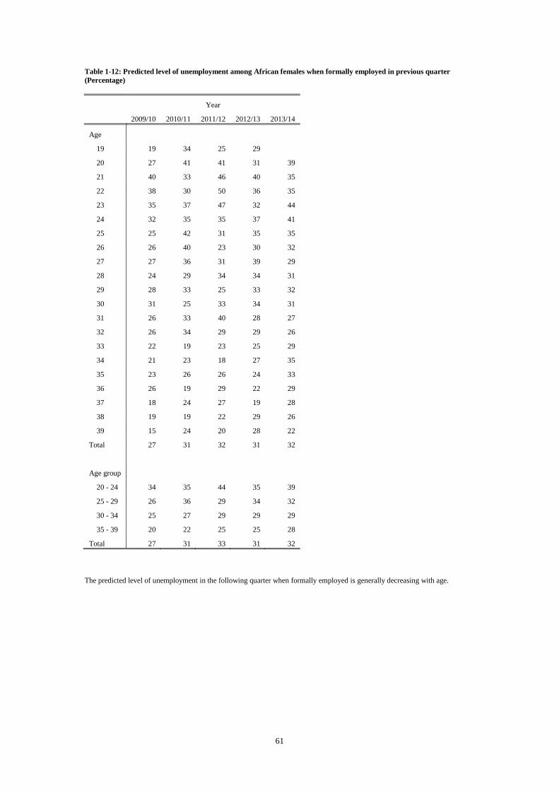
61

Table 1-12: Predicted level of unemployment among African females when formally employed in previous quarter

(Percentage)

Year

2009/10 2010/11 2011/12 2012/13 2013/14

Age

19 19 34 25 29

20 27 41 41 31 39

21 40 33 46 40 35

22 38 30 50 36 35

23 35 37 47 32 44

24 32 35 35 37 41

25 25 42 31 35 35

26 26 40 23 30 32

27 27 36 31 39 29

28 24 29 34 34 31

29 28 33 25 33 32

30 31 25 33 34 31

31 26 33 40 28 27

32 26 34 29 29 26

33 22 19 23 25 29

34 21 23 18 27 35

35 23 26 26 24 33

36 26 19 29 22 29

37 18 24 27 19 28

38 19 19 22 29 26

39 15 24 20 28 22

Total 27 31 32 31 32

Age group

20 - 24 34 35 44 35 39

25 - 29 26 36 29 34 32

30 - 34 25 27 29 29 29

35 - 39 20 22 25 25 28

Total 27 31 33 31 32

The predicted level of unemployment in the following quarter when formally employed is generally decreasing with age.

62

Table 1-13: Predicted level of unemployment among African males when informally employed in previous quarter

(Percentage)

Year

2009/10 2010/11 2011/12 2012/13 2013/14

Age

19 23 26 21 34 32

20 40 33 28 36 49

21 38 46 39 46 49

22 41 45 46 52 46

23 37 45 40 38 42

24 36 41 35 34 48

25 31 37 36 36 39

26 33 34 42 35 34

27 29 33 33 33 33

28 27 31 29 31 28

29 23 28 24 28 26

30 27 27 29 25 33

31 24 23 30 27 30

32 21 20 29 30 24

33 21 16 25 31 22

34 16 23 23 22 23

35 22 21 23 23 16

36 17 21 23 18 23

37 19 23 20 20 23

38 23 21 23 18 15

39 18 23 22 24 21

Total 28 31 31 32 33

Age group

20 - 24 39 41 38 42 47

25 - 29 29 33 33 32 32

30 - 34 22 22 27 27 27

35 - 39 19 22 22 21 20

Total 29 32 31 32 34

The predicted level of unemployment in the following quarter when informally employed is generally decreasing with age.

63

Table 1-14: Predicted level of unemployment among African females when informally employed in previous quarter

(Percentage)

Year

2009/10 2010/11 2011/12 2012/13 2013/14

Age

19 25 59 37 25

20 32 55 40 35 32

21 35 46 41 42 43

22 37 47 41 42 40

23 34 41 49 51 40

24 45 36 43 57 35

25 45 37 36 51 38

26 36 44 40 39 40

27 42 42 37 40 41

28 38 35 33 32 39

29 37 41 40 32 33

30 31 45 39 40 33

31 28 32 38 35 33

32 27 31 36 41 32

33 30 22 32 33 32

34 31 27 22 30 33

35 23 36 28 34 31

36 27 30 29 31 37

37 24 31 30 27 32

38 24 28 36 23 28

39 20 26 33 25 24

Total 33 39 37 37 35

Age group

20 - 24 37 45 43 45 38

25 - 29 40 40 37 39 38

30 - 34 29 32 34 36 33

35 - 39 24 30 31 28 30

Total 33 38 37 38 35

The predicted level of unemployment in the following quarter when informally employed is generally decreasing with age.

64

Table 1-15: Predicted level of unemployment among African males when long term unemployed in previous quarter

(Percentage)

Year

2009/10 2010/11 2011/12 2012/13 2013/14

Age

19 39 36 41 33 36

20 51 52 46 51 49

21 62 57 52 62 53

22 57 54 58 61 61

23 61 60 64 59 62

24 58 58 62 63 57

25 62 54 57 64 52

26 60 48 53 59 54

27 59 51 50 49 48

28 51 46 51 46 45

29 42 45 47 54 48

30 50 36 44 57 46

31 52 39 44 41 36

32 45 36 47 35 41

33 44 41 45 32 33

34 41 41 36 36 29

35 44 39 37 31 47

36 48 36 38 40 40

37 34 32 39 38 45

38 36 33 28 34 53

39 34 34 28 39 42

Total 50 46 48 48 47

Age group

20 - 24 57 56 56 59 56

25 - 29 55 49 52 54 50

30 - 34 46 38 43 41 37

35 - 39 39 35 35 36 45

Total 51 47 48 49 48

The predicted level of unemployment in the following quarter when long term unemployed is generally decreasing with age.

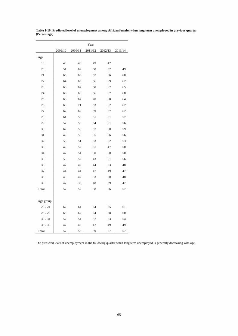
65

Table 1-16: Predicted level of unemployment among African females when long term unemployed in previous quarter

(Percentage)

Year

2009/10 2010/11 2011/12 2012/13 2013/14

Age

19 49 46 49 42

20 51 62 58 57 49

21 65 63 67 66 60

22 64 65 66 69 62

23 66 67 60 67 65

24 66 66 66 67 68

25 66 67 70 68 64

26 68 71 63 62 62

27 62 62 59 57 62

28 61 55 61 51 57

29 57 55 64 51 56

30 62 56 57 60 59

31 49 56 55 56 56

32 53 51 63 52 53

33 49 52 61 47 50

34 47 54 50 50 50

35 55 52 43 51 56

36 47 42 44 53 48

37 44 44 47 49 47

38 40 47 53 50 48

39 47 38 48 39 47

Total 57 57 58 56 57

Age group

20 - 24 62 64 64 65 61

25 - 29 63 62 64 58 60

30 - 34 52 54 57 53 54

35 - 39 47 45 47 49 49

Total 57 58 59 57 57

The predicted level of unemployment in the following quarter when long term unemployed is generally decreasing with age.

66

Table 1-17: Predicted level of unemployment among African males when short term unemployed in previous quarter

(Percentage)

Year

2009/10 2010/11 2011/12 2012/13 2013/14

Age

19 32 34 36 30 36

20 52 48 47 44 48

21 52 52 44 51 52

22 51 52 50 55 57

23 54 52 52 54 60

24 46 50 60 55 59

25 55 53 52 57 52

26 50 48 46 49 44

27 45 47 45 44 44

28 44 41 41 46 39

29 36 43 38 45 34

30 38 38 35 49 38

31 40 36 40 41 36

32 38 33 39 34 37

33 37 34 35 26 33

34 38 37 29 33 29

35 35 32 27 28 38

36 34 34 30 28 29

37 24 29 30 25 35

38 29 31 25 25 38

39 25 30 29 31 27

Total 42 42 41 42 43

Age group

20 - 24 51 51 50 51 55

25 - 29 46 47 45 48 43

30 - 34 38 36 36 37 35

35 - 39 29 31 28 27 33

Total 43 43 42 43 43

The predicted level of unemployment in the following quarter when short term unemployed is generally decreasing with age.

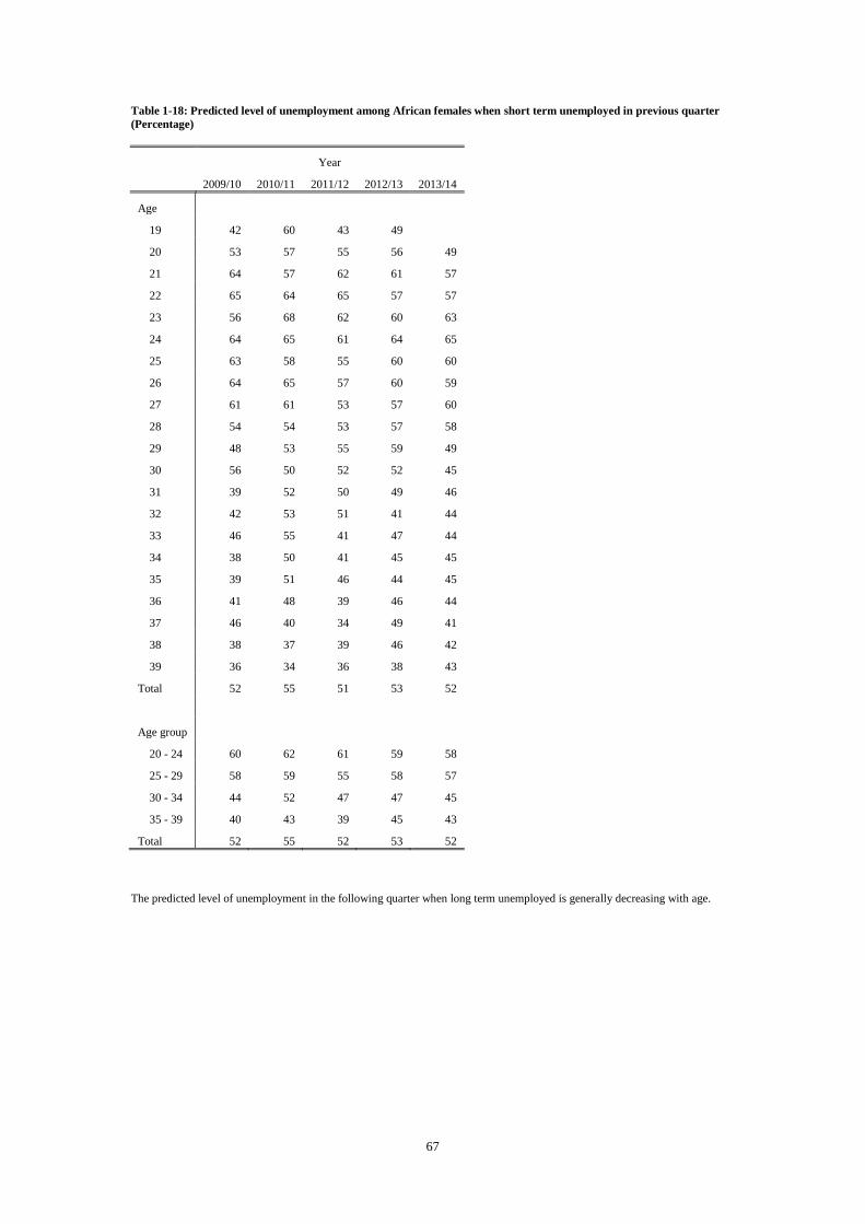
67

Table 1-18: Predicted level of unemployment among African females when short term unemployed in previous quarter

(Percentage)

Year

2009/10 2010/11 2011/12 2012/13 2013/14

Age

19 42 60 43 49

20 53 57 55 56 49

21 64 57 62 61 57

22 65 64 65 57 57

23 56 68 62 60 63

24 64 65 61 64 65

25 63 58 55 60 60

26 64 65 57 60 59

27 61 61 53 57 60

28 54 54 53 57 58

29 48 53 55 59 49

30 56 50 52 52 45

31 39 52 50 49 46

32 42 53 51 41 44

33 46 55 41 47 44

34 38 50 41 45 45

35 39 51 46 44 45

36 41 48 39 46 44

37 46 40 34 49 41

38 38 37 39 46 42

39 36 34 36 38 43

Total 52 55 51 53 52

Age group

20 - 24 60 62 61 59 58

25 - 29 58 59 55 58 57

30 - 34 44 52 47 47 45

35 - 39 40 43 39 45 43

Total 52 55 52 53 52

The predicted level of unemployment in the following quarter when long term unemployed is generally decreasing with age.

68

We now investigate the level of state dependence in unemployment at different ages with

references to both formal and informal employment. Table 1-19 to Table 1-28 present our

estimates of state dependence in unemployment, both for individuals that have been

unemployed for less than a year and those have never been employed or have been

unemployed for more than a year, at different ages. These estimates include the average

difference in the predicted level of unemployment (in the following quarter) from formal

employment and the predicted level of unemployment from long term unemployment; the

difference in the predicted level of unemployment from informal employment and the

predicted level of unemployment from long term unemployment; the difference in the

predicted level of unemployment from formal employment and the predicted level of

unemployment from short term unemployment; the difference in the predicted level of

unemployment from informal employment and the predicted level of unemployment from

short term unemployment; and the average difference in the predicted level of unemployment

from short term unemployment and the predicted level of unemployment from long term

unemployment. Note that a negative figure reflects state dependence in unemployment, and

that larger differences correspond to higher levels of state dependence. Thus if the average

difference in the predicted level of unemployment (in the following quarter) from formal

employment and the predicted level of unemployment from long term unemployment is -20,

workers that were unemployed in the preceding quarter are, ceteris paribus, 20%-points more

likely to unemployed than if they had been formally employed in the preceding quarter.

Our estimates of state dependence in unemployment are, again generally, similar among those

workers in the age group 25 to 29 and those aged 20 to 24. However these estimates also vary

considerably within these age-groups, between age-groups, and from year to year. For

example in 2013/2014 state dependence in unemployment is more pronounced for those aged

35 to 39 than it is for those aged 30 to 34. Table 1-15 suggests that this may be because those

workers aged 35 to 39 were less likely to transition out of unemployment than those aged 30

to 34. The increase in the level of state dependence in unemployment within the age-group 35

69

to 39 is also consistent across the different ages in this group and it is consequently unlikely

that the estimates are merely a feature of the QLFS sample draws in this year17. Regrettably

the bootstrapped confidence intervals for these estimates (which we do not report) are large

and we are unable to conclude that there are statistically significant differences in the level of

state dependence in unemployment between age and across these periods.

17 This may, in part, be due to the South African Government’s most recent effort to assist unemployed youth.

While we cannot rule out that this is due to the particular sample draw, the Youth Employment Tax Incentive

(ETI) may have had an effect on these outcomes. Alternately those aged 35 to 39 may have been less likely to

move out of the labour force. We are unaware of any other intervention that is associated with this age-group (or

birth-cohort).

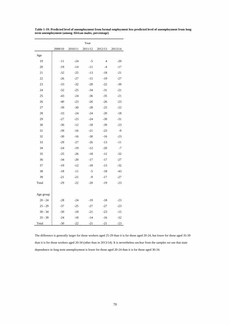
70

Table 1-19: Predicted level of unemployment from formal employment less predicted level of unemployment from long

term unemployment (among African males, percentage)

Year

2009/10 2010/11 2011/12 2012/13 2013/14

Age

19 -11 -24 -5 4 -20

20 -19 -14 -11 -4 -17

21 -32 -25 -13 -18 -21

22 -26 -27 -15 -19 -27

23 -33 -32 -28 -22 -30

24 -32 -25 -34 -31 -21

25 -43 -24 -36 -35 -21

26 -40 -23 -26 -26 -23

27 -39 -30 -28 -25 -22

28 -33 -24 -24 -20 -18

29 -27 -23 -24 -30 -31

30 -30 -12 -18 -39 -23

31 -39 -16 -21 -23 -9

32 -30 -16 -30 -16 -23

33 -29 -27 -26 -13 -11

34 -24 -19 -12 -20 -7

35 -25 -26 -18 -12 -32

36 -34 -20 -17 -17 -27

37 -19 -12 -18 -13 -32

38 -18 -11 -5 -18 -43

39 -21 -21 -9 -17 -27

Total -29 -22 -20 -19 -23

Age group

20 - 24 -28 -24 -19 -18 -23

25 - 29 -37 -25 -27 -27 -23

30 - 34 -30 -18 -21 -23 -15

35 - 39 -24 -18 -14 -16 -32

Total -30 -22 -21 -21 -23

The difference is generally larger for those workers aged 25-29 than it is for those aged 20-24, but lower for those aged 35-39

than it is for those workers aged 20-34 (other than in 2013/14). It is nevertheless unclear from the samples we use that state

dependence in long term unemployment is lower for those aged 20-24 than it is for those aged 30-34.

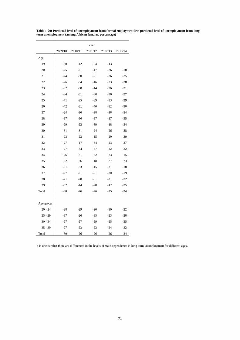
71

Table 1-20: Predicted level of unemployment from formal employment less predicted level of unemployment from long

term unemployment (among African females, percentage)

Year

2009/10 2010/11 2011/12 2012/13 2013/14

Age

19 -30 -12 -24 -13

20 -25 -21 -17 -26 -10

21 -24 -30 -21 -26 -25

22 -26 -34 -16 -33 -28

23 -32 -30 -14 -36 -21

24 -34 -31 -30 -30 -27

25 -41 -25 -39 -33 -29

26 -42 -31 -40 -32 -30

27 -34 -26 -28 -18 -34

28 -37 -26 -27 -17 -25

29 -29 -22 -39 -18 -24

30 -31 -31 -24 -26 -28

31 -23 -23 -15 -29 -30

32 -27 -17 -34 -23 -27

33 -27 -34 -37 -22 -22

34 -26 -31 -32 -23 -15

35 -32 -26 -18 -27 -23

36 -21 -23 -15 -31 -18

37 -27 -21 -21 -30 -19

38 -21 -28 -31 -21 -22

39 -32 -14 -28 -12 -25

Total -30 -26 -26 -25 -24

Age group

20 - 24 -28 -29 -20 -30 -22

25 - 29 -37 -26 -35 -23 -28

30 - 34 -27 -27 -29 -25 -25

35 - 39 -27 -23 -22 -24 -22

Total -30 -26 -26 -26 -24

It is unclear that there are differences in the levels of state dependence in long term unemployment for different ages.

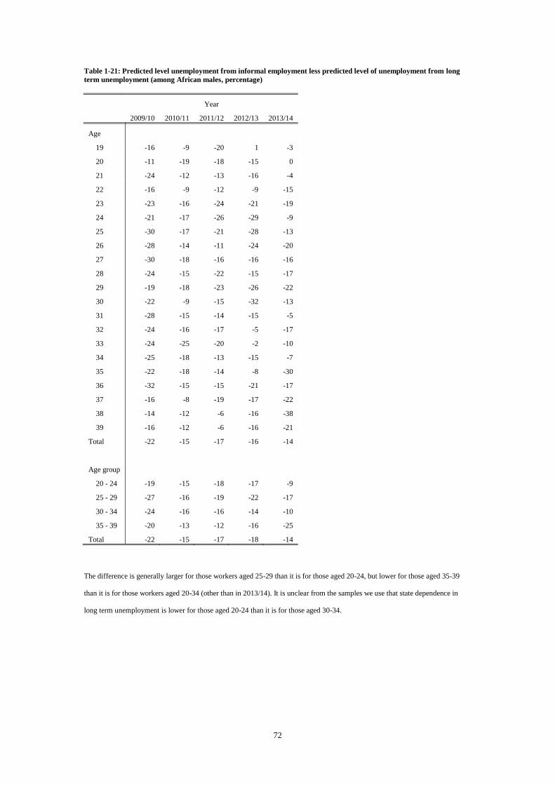
72

Table 1-21: Predicted level unemployment from informal employment less predicted level of unemployment from long

term unemployment (among African males, percentage)

Year

2009/10 2010/11 2011/12 2012/13 2013/14

Age

19 -16 -9 -20 1 -3

20 -11 -19 -18 -15 0

21 -24 -12 -13 -16 -4

22 -16 -9 -12 -9 -15

23 -23 -16 -24 -21 -19

24 -21 -17 -26 -29 -9

25 -30 -17 -21 -28 -13

26 -28 -14 -11 -24 -20

27 -30 -18 -16 -16 -16

28 -24 -15 -22 -15 -17

29 -19 -18 -23 -26 -22

30 -22 -9 -15 -32 -13

31 -28 -15 -14 -15 -5

32 -24 -16 -17 -5 -17

33 -24 -25 -20 -2 -10

34 -25 -18 -13 -15 -7

35 -22 -18 -14 -8 -30

36 -32 -15 -15 -21 -17

37 -16 -8 -19 -17 -22

38 -14 -12 -6 -16 -38

39 -16 -12 -6 -16 -21

Total -22 -15 -17 -16 -14

Age group

20 - 24 -19 -15 -18 -17 -9

25 - 29 -27 -16 -19 -22 -17

30 - 34 -24 -16 -16 -14 -10

35 - 39 -20 -13 -12 -16 -25

Total -22 -15 -17 -18 -14

The difference is generally larger for those workers aged 25-29 than it is for those aged 20-24, but lower for those aged 35-39

than it is for those workers aged 20-34 (other than in 2013/14). It is unclear from the samples we use that state dependence in

long term unemployment is lower for those aged 20-24 than it is for those aged 30-34.

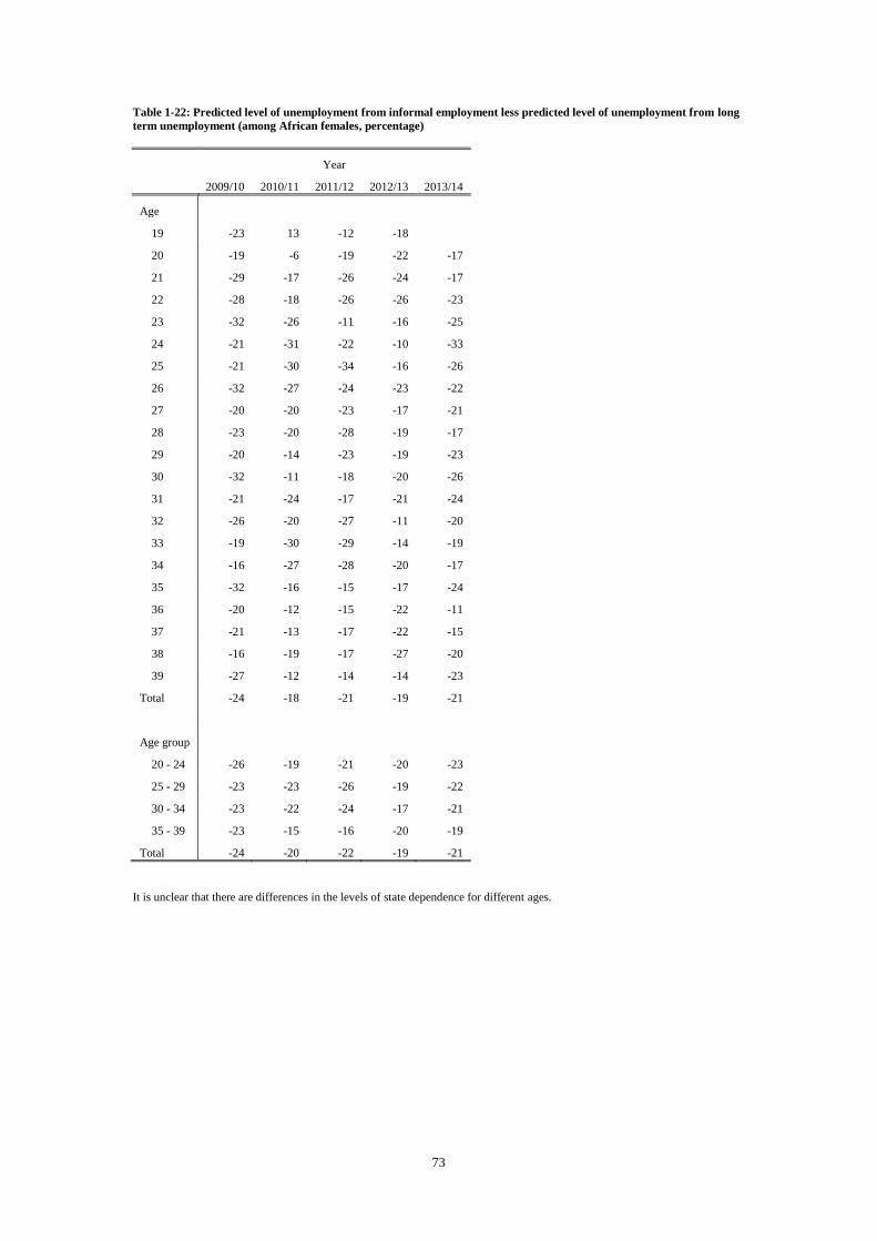
73

Table 1-22: Predicted level of unemployment from informal employment less predicted level of unemployment from long

term unemployment (among African females, percentage)

Year

2009/10 2010/11 2011/12 2012/13 2013/14

Age

19 -23 13 -12 -18

20 -19 -6 -19 -22 -17

21 -29 -17 -26 -24 -17

22 -28 -18 -26 -26 -23

23 -32 -26 -11 -16 -25

24 -21 -31 -22 -10 -33

25 -21 -30 -34 -16 -26

26 -32 -27 -24 -23 -22

27 -20 -20 -23 -17 -21

28 -23 -20 -28 -19 -17

29 -20 -14 -23 -19 -23

30 -32 -11 -18 -20 -26

31 -21 -24 -17 -21 -24

32 -26 -20 -27 -11 -20

33 -19 -30 -29 -14 -19

34 -16 -27 -28 -20 -17

35 -32 -16 -15 -17 -24

36 -20 -12 -15 -22 -11

37 -21 -13 -17 -22 -15

38 -16 -19 -17 -27 -20

39 -27 -12 -14 -14 -23

Total -24 -18 -21 -19 -21

Age group

20 - 24 -26 -19 -21 -20 -23

25 - 29 -23 -23 -26 -19 -22

30 - 34 -23 -22 -24 -17 -21

35 - 39 -23 -15 -16 -20 -19

Total -24 -20 -22 -19 -21

It is unclear that there are differences in the levels of state dependence for different ages.

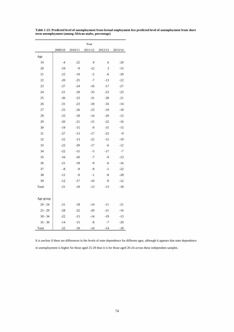
74

Table 1-23: Predicted level of unemployment from formal employment less predicted level of unemployment from short

term unemployment (among African males, percentage)

Year

2009/10 2010/11 2011/12 2012/13 2013/14

Age

19 -4 -22 0 6 -20

20 -19 -9 -12 3 -15

21 -22 -19 -5 -6 -20

22 -20 -25 -7 -13 -22

23 -27 -24 -16 -17 -27

24 -21 -18 -33 -23 -23

25 -36 -23 -31 -28 -21

26 -31 -23 -18 -16 -14

27 -25 -26 -23 -19 -18

28 -25 -18 -14 -20 -12

29 -20 -21 -15 -22 -16

30 -19 -15 -9 -31 -15

31 -27 -13 -17 -23 -9

32 -22 -13 -22 -15 -19

33 -22 -20 -17 -6 -12

34 -22 -15 -5 -17 -7

35 -16 -20 -7 -9 -23

36 -21 -18 -9 -6 -16

37 -8 -9 -9 -1 -22

38 -12 -9 -1 -8 -28

39 -12 -17 -10 -9 -12

Total -21 -18 -13 -13 -18

Age group

20 - 24 -21 -18 -14 -11 -21

25 - 29 -28 -22 -20 -21 -16

30 - 34 -22 -15 -14 -19 -13

35 - 39 -14 -15 -8 -7 -20

Total -22 -18 -14 -14 -18

It is unclear if there are differences in the levels of state dependence for different ages, although it appears that state dependence

in unemployment is higher for those aged 25-29 than it is for those aged 20-24 across these independent samples.

75

Table 1-24: Predicted level of unemployment from formal employment less predicted level of unemployment from short

term unemployment (among African females, percentage)

Year

2009/10 2010/11 2011/12 2012/13 2013/14

Age

19 -23 -26 -18 -20

20 -27 -16 -14 -24 -10

21 -24 -24 -16 -21 -22

22 -27 -34 -15 -22 -22

23 -21 -31 -16 -28 -19

24 -31 -30 -26 -27 -25

25 -38 -16 -25 -25 -26

26 -37 -25 -33 -29 -27

27 -33 -25 -22 -18 -31

28 -30 -25 -19 -23 -27

29 -20 -21 -30 -26 -17

30 -25 -26 -18 -18 -14

31 -13 -18 -10 -22 -19

32 -16 -18 -22 -12 -18

33 -24 -36 -18 -22 -16

34 -17 -27 -23 -18 -10

35 -17 -25 -20 -19 -13

36 -15 -28 -11 -24 -15

37 -28 -17 -7 -30 -13

38 -19 -18 -17 -17 -16

39 -21 -10 -16 -11 -21

Total -25 -24 -19 -22 -19

Age group

20 - 24 -26 -27 -17 -24 -19

25 - 29 -32 -22 -26 -24 -26

30 - 34 -19 -25 -18 -18 -16

35 - 39 -20 -20 -14 -20 -15

Total -25 -24 -19 -22 -19

It is unclear if there are differences in the levels of state dependence for different ages, although it appears that state dependence

in unemployment is generally higher for those aged 25-29 than it is for those aged 20-24 across these independent samples.

76

Table 1-25: Predicted level of unemployment from informal employment less predicted level of unemployment from short

term unemployment (among African males, percentage)

Year

2009/10 2010/11 2011/12 2012/13 2013/14

Age

19 -9 -8 -15 4 -3

20 -11 -15 -18 -8 2

21 -14 -6 -5 -4 -3

22 -10 -7 -4 -3 -10

23 -16 -7 -12 -16 -17

24 -10 -10 -25 -21 -11

25 -23 -16 -16 -21 -13

26 -18 -14 -4 -14 -11

27 -16 -14 -12 -11 -11

28 -17 -9 -12 -15 -11

29 -13 -15 -15 -18 -8

30 -11 -12 -6 -24 -5

31 -16 -13 -10 -14 -6

32 -17 -13 -10 -4 -13

33 -16 -18 -10 4 -11

34 -23 -14 -6 -12 -7

35 -13 -11 -4 -5 -21

36 -18 -13 -6 -10 -6

37 -5 -6 -10 -5 -12

38 -7 -10 -2 -6 -23

39 -7 -7 -7 -7 -6

Total -14 -11 -11 -10 -9

Age group

20 - 24 -12 -9 -12 -10 -8

25 - 29 -17 -14 -12 -16 -11

30 - 34 -16 -14 -8 -11 -8

35 - 39 -10 -10 -6 -7 -14

Total -14 -11 -10 -11 -10

It is unclear that there are differences in the levels of state dependence for different ages.

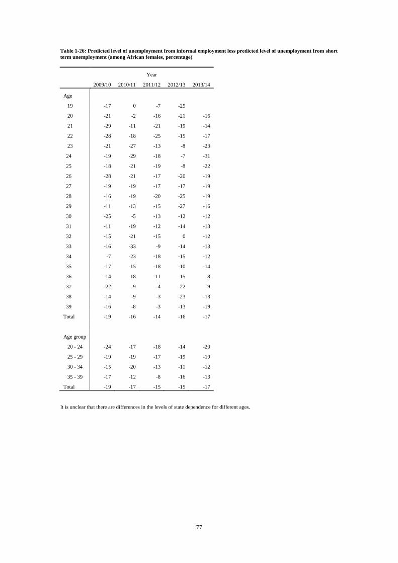
77

Table 1-26: Predicted level of unemployment from informal employment less predicted level of unemployment from short

term unemployment (among African females, percentage)

Year

2009/10 2010/11 2011/12 2012/13 2013/14

Age

19 -17 0 -7 -25

20 -21 -2 -16 -21 -16

21 -29 -11 -21 -19 -14

22 -28 -18 -25 -15 -17

23 -21 -27 -13 -8 -23

24 -19 -29 -18 -7 -31

25 -18 -21 -19 -8 -22

26 -28 -21 -17 -20 -19

27 -19 -19 -17 -17 -19

28 -16 -19 -20 -25 -19

29 -11 -13 -15 -27 -16

30 -25 -5 -13 -12 -12

31 -11 -19 -12 -14 -13

32 -15 -21 -15 0 -12

33 -16 -33 -9 -14 -13

34 -7 -23 -18 -15 -12

35 -17 -15 -18 -10 -14

36 -14 -18 -11 -15 -8

37 -22 -9 -4 -22 -9

38 -14 -9 -3 -23 -13

39 -16 -8 -3 -13 -19

Total -19 -16 -14 -16 -17

Age group

20 - 24 -24 -17 -18 -14 -20

25 - 29 -19 -19 -17 -19 -19

30 - 34 -15 -20 -13 -11 -12

35 - 39 -17 -12 -8 -16 -13

Total -19 -17 -15 -15 -17

It is unclear that there are differences in the levels of state dependence for different ages.

78

Table 1-27: Predicted level of unemployment from long term unemployment less predicted level of unemployment from

short term unemployment (among African males, percentage)

Year

2009/10 2010/11 2011/12 2012/13 2013/14

Age

19 -7 -2 -5 -3 0

20 0 -4 1 -7 -2

21 -10 -6 -8 -11 -1

22 -6 -2 -8 -6 -4

23 -7 -9 -12 -5 -2

24 -12 -8 -1 -8 2

25 -7 -1 -5 -7 0

26 -10 0 -7 -10 -9

27 -14 -4 -5 -5 -5

28 -7 -6 -10 0 -6

29 -6 -2 -9 -8 -15

30 -11 2 -9 -7 -8

31 -12 -3 -4 0 0

32 -7 -3 -8 -1 -4

33 -7 -7 -10 -6 1

34 -3 -4 -7 -3 0

35 -9 -7 -11 -3 -9

36 -14 -2 -8 -11 -11

37 -11 -2 -9 -12 -10

38 -7 -2 -4 -10 -14

39 -9 -4 1 -8 -14

Total -8 -4 -6 -6 -5

Age group

20 - 24 -6 -6 -6 -8 -1

25 - 29 -9 -3 -7 -6 -7

30 - 34 -8 -2 -7 -4 -2

35 - 39 -10 -3 -6 -9 -12

Total -8 -4 -7 -7 -5

It is unclear that there are differences in the levels of state dependence for different ages.

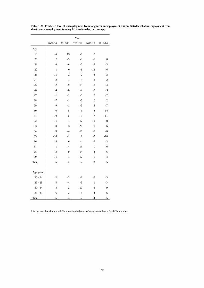
79

Table 1-28: Predicted level of unemployment from long term unemployment less predicted level of unemployment from

short term unemployment (among African females, percentage)

Year

2009/10 2010/11 2011/12 2012/13 2013/14

Age

19 -6 13 -6 7

20 2 -5 -3 -1 0

21 0 -6 -5 -5 -3

22 1 0 -1 -12 -6

23 -11 2 2 -8 -2

24 -2 -1 -5 -3 -2

25 -2 -9 -15 -8 -4

26 -4 -6 -7 -3 -3

27 -1 -1 -6 0 -2

28 -7 -1 -8 6 2

29 -9 -1 -9 8 -7

30 -6 -5 -6 -8 -14

31 -10 -5 -5 -7 -11

32 -11 1 -12 -11 -8

33 -3 3 -20 0 -6

34 -9 -4 -10 -5 -6

35 -16 -1 2 -7 -10

36 -5 6 -4 -7 -3

37 1 -4 -13 0 -6

38 -3 -9 -14 -4 -6

39 -11 -4 -12 -1 -4

Total -5 -2 -7 -3 -5

Age group

20 - 24 -2 -2 -2 -6 -3

25 - 29 -5 -4 -9 1 -3

30 - 34 -8 -2 -10 -6 -9

35 - 39 -6 -2 -8 -4 -6

Total -5 -3 -7 -4 -5

It is unclear that there are differences in the levels of state dependence for different ages.

80

Discussion and conclusion

The estimates we presented in the previous section show that there is state dependence in both

long term and short term unemployment among young African South Africans. There also

appears to be considerable heterogeneity within the different age groups that Lam et al.

(2007) define and between years. We are however unable to conclude that state dependence

in unemployment is significantly different between workers aged 20 to 24, 25 to 29, 30 to 34

and 35 to 39.

It is transparent though that the level of state dependence in unemployment is not, as we

initially expected, necessarily higher among those aged 20 to 24 than it is for those aged 25 to

29. This is principally due to the pattern across these independent samples that younger

workers are more likely to transition from employment into unemployment than their older

counterparts. One explanation for this finding is that younger workers may be more exposed

to lower paying or less appealing work than their older counterparts. This may explain why

our estimates of state dependence in unemployment at different ages are closely associated

with labour force participation rates by age. However we also show that the trajectory of the

predictions of unemployment by age correspond for both formal and informal employment

and for short term and long term unemployment.

A second explanation for why young workers appear to exit employment more frequently

than their older counterparts is that they may be employed in short term jobs. The data we use

does not as mentioned allow us to calculate how long an employed worker has been in

employment. However if younger workers are more likely to be employed in short term jobs

it is not clear why this is the case (particularly when they are formally employed) and this

does not alter the conclusions we draw on the levels of state dependence in unemployment.

In our view the most appealing explanation for the similarity in the levels of state dependence

in long term unemployment among workers in their twenties is that workers become more

productive as they grow older. This is why they are less likely to transition out of

81

employment. It just happens that, at least in South Africa, long term unemployed workers in

their mid to late twenties may find it more difficult to find work than they should. We are

therefore tempted to argue, in the absence of more rigorous experimental evidence, that short

term interventions that are intended to reduce long term unemployment among youth should

also (continue to) target workers aged 25 to 29. However there is considerable state

dependence in both short term and long term unemployment even among workers aged 35 to

39. Indeed our point estimates for 2013/2014 show us that among African males state

dependence in both long term and short term unemployment is more pronounced in this age-

group than for younger workers.

82

References

1. Arulampalam, W., Booth, A. L., and Taylor, M. P. (2000). Unemployment

persistence. Oxford Economic Papers, 52(1), 24-50.

2. Audas, R., Berde, E., and Dolton, P. (2005). Youth unemployment and labour market

transitions in Hungary. Education Economics, 13(1), 1-25.

3. Banerjee, A., Galiani, S., Levinsohn, J., McLaren, Z., and Woolard, I. (2008). Why

has unemployment risen in the new South Africa? Economics of Transition, 16(4),

715-740.

4. Betcherman, G., Godfrey, M., Puerto, S., Rother, F., and Stavreska, A. (2007). A

review of interventions to support young workers: Findings of the youth employment

inventory. World Bank Social Protection Discussion Paper, 715.

5. Buddelmeyer, H., and Verick, S. (2011). New insights into the dynamics of the South

African labour market. Asian Meeting of Econometric Society, 2011.

6. Burger, R., and Von Fintel, D. (2009). Determining the causes of the rising South

African unemployment rate: An age, period and generational analysis. Economic

Research Southern Africa (ERSA) Working Papers, (158).

7. Burgess, S., Propper, C., Rees, H., and Shearer, A. (2003). The class of 1981: the

effects of early career unemployment on subsequent unemployment experiences.

Labour Economics, 10(3), 291-309.

8. Carling, K., and Larsson, L. (2005). Does early intervention help the unemployed

youth?. Labour

9. Cockx, Bart, and Matteo Picchio. (2013). Scarring effects of remaining unemployed

for long term unemployed school-leavers. Journal of the Royal Statistical Society:

Series A (Statistics in Society) 176.4 (2013): 951-980.

10. Doiron, D., and Gørgens, T. (2008). State dependence in youth labor market

experiences, and the evaluation of policy interventions. Journal of Econometrics,

145(1), 81-97.

83

11. Essers, D. (2013). South African labour market transitions during the global financial

and economic crisis: Micro-level evidence from the NIDS panel and matched QLFS

cross-sections. IOB Working Papers 2013.12, Universiteit Antwerpen, Institute of

Development Policy and Management (IOB).

12. Fares, J., and Tiongson, E. (2007). Youth unemployment, labor market transitions,

and scarring: evidence from Bosnia and Herzegovina, 2001-04 (Vol. 4183). World

Bank Publications.

13. Heckman, J. J. (1981). Heterogeneity and state dependence. In Studies in labor

markets (pp. 91-140). University of Chicago Press.

14. Heckman, J. J., and Borjas, G. J. (1980). Does unemployment cause future

unemployment? Definitions, questions and answers from a continuous time model of

heterogeneity and state dependence. Economica, 47(187), 247-283.

15. Honoré, B. E., and Kyriazidou, E. (2000). Panel data discrete choice models with

lagged dependent variables. Econometrica, 839-874.

16. ILO. (2013). Global Employment Trends for Youth 2013: A generation at risk.

International Labour Office – Geneva

17. Jacobson, L. S., LaLonde, R. J., and Sullivan, D. G. (1993). Earnings losses of

displaced workers. The American Economic Review, 685-709.

18. Jenkins, S. P. (2013). On state dependence: a case for two-handed economists.

LASER.

19. Kingdon, G. G., and Knight, J. (2004). Unemployment in South Africa: The nature of

the beast. World development, 32(3), 391-408.

20. Lam, D., Leibbrandt, M. and Mlatsheni, C. (2007). Dynamics of Labor Market Entry

and Youth Unemployment in South Africa: Evidence from the Cape Area Panel

Study. IPC Working Paper Series Number 34

21. Magnac, T. (2000). Subsidised training and youth employment: distinguishing

unobserved heterogeneity from state dependence in labour market histories. The

Economic Journal, 110(466), 805-837.

84

22. Mariotti, M., and Meinecke, J. (2014). Partial Identification and Bound Estimation of

the Average Treatment Effect of Education on Earnings for South Africa. Oxford

Bulletin of Economics and Statistics.

23. Mlatsheni, C. and Rospabe, S. (2002). Why is youth unemployment so high and

unequally spread in South Africa? DPRU Working Paper No. 02/65.

24. Mroz, T. A., and Savage, T. H. (2006). The long term effects of youth

unemployment. Journal of Human Resources, 41(2), 259-293.

25. National Youth Policy. (2008). National Youth Policy 2009-2014. Republic of South

Africa.

26. Rabe-Hesketh, S., and Skrondal, A. (2013). Avoiding biased versions of

Wooldridge’s simple solution to the initial conditions problem. Economics Letters,

120(2), 346-349.

27. Ranchhod, V., and Finn, A. (2014). Estimating the short run effects of South Africa's

Employment Tax Incentive on youth employment probabilities using a difference-in-

differences approach.

28. Skrondal, A., and Rabe-Hesketh, S. (2014). Handling initial conditions and

endogenous covariates in dynamic/transition models for binary data with unobserved

heterogeneity. Journal of the Royal Statistical Society: Series C (Applied Statistics).

29. Stats SA. (2014). Quarterly Labour Force Survey Quarter 2, 2014: Metadata/Statistics

South Africa. Pretoria: Statistics South Africa, 2014. [Statistical Release: P0211

(2014)]. Supplied by the South African Data Archive (SADA). www.sada.nrf.org

30. Stewart, M. B. (2007). The interrelated dynamics of unemployment and low‐wage

employment. Journal of applied econometrics, 22(3), 511-531.

31. Topel, R. H. (1990). Specific capital, mobility, and wages: Wages rise with job

seniority (No. w3294). National Bureau of Economic Research.

32. Wooldridge, J. M. (2005). Simple solutions to the initial conditions problem in

dynamic, nonlinear panel data models with unobserved heterogeneity. Journal of

Applied Econometrics, 20(1), 39-54.

85

Appendix

Table A1-1: Number of observations by year

Year

2008 2009 2010 2011 2012 2013 2014 Total

Age

17 31 24 11 17 11 14 0 108

18 1312 1589 1834 1699 1676 1694 285 10089

19 3519 5531 5419 5033 4844 4854 1836 31036

20 3478 5218 5362 4713 4851 4611 1801 30034

21 3176 4863 4953 4714 4701 4713 1800 28920

22 3038 4602 4589 4289 4528 4450 `1658 27154

23 2925 4506 4429 4079 4204 4188 1715 26046

24 2623 4382 4266 3914 4164 4018 1509 24876

25 2824 4171 4026 3899 3795 4000 1590 24305

26 2526 4198 3821 3704 3738 3836 1421 23244

27 2262 3842 3896 3480 3701 3759 1391 22331

28 2475 3574 3502 3559 3702 3758 1463 22033

29 2119 3565 3177 3261 3607 3611 1361 20701

30 2103 3415 3356 2998 3398 3686 1294 20250

31 2031 3073 3018 3057 3059 3275 1274 18787

32 2097 3266 2905 2779 3354 3211 1115 18727

33 2075 3163 2760 2535 2972 3148 1255 17908

34 1965 3114 2953 2591 2833 2884 1184 17524

35 1890 2855 2878 2731 2807 2831 1030 17022

36 1847 3114 2774 2648 2955 2656 944 16938

37 1674 2942 2827 2503 2728 2818 956 16448

38 1983 2682 2639 2536 2671 2813 961 16285

39 1835 3019 2474 2355 2822 2712 1032 16249

40 428 922 983 705 958 954 519 5469

41 8 12 18 4 10 5 7 64

Total 52244 81642 78870 73803 78089 78499 29401 472548

86

Table A1-2: Estimates for African males age 19 to 24 in 2013/14 (Random-effects Probit)

Age

19 20 21 22 23 24

Lagged state

(Reference long term unemployed)

Missing -0.987*** -0.752*** -0.461*** -0.654*** -0.832*** -0.505***

(0.354) (0.203) (0.178) (0.161) (0.175) (0.176)

NEA -2.020*** -1.874*** -1.404*** -1.382*** -1.513*** -1.743***

(0.325) (0.198) (0.170) (0.176) (0.218) (0.207)

Short term unemployed 0.009 -0.104 -0.052 -0.198 -0.100 0.104

(0.466) (0.277) (0.208) (0.201) (0.182) (0.200)

Formal employed -1.801*** -1.125** -1.144*** -1.271*** -1.292*** -1.027***

(0.584) (0.472) (0.358) (0.274) (0.300) (0.195)

Informal employed -0.250 0.005 -0.198 -0.685*** -0.831*** -0.439*

(0.516) (0.328) (0.270) (0.220) (0.234) (0.248)

Initial state

(Reference long term unemployed)

Missing -3.777*** -2.931*** -2.000*** -1.866*** -1.730*** -1.992***

(0.762) (0.445) (0.269) (0.273) (0.268) (0.318)

NEA -3.418*** -2.489*** -1.790*** -1.397*** -1.180*** -0.839***

(0.682) (0.401) (0.236) (0.244) (0.286) (0.291)

Short term unemployed -0.308 -0.212 -0.114 -0.162 -0.259 -0.518**

(0.616) (0.446) (0.251) (0.242) (0.215) (0.251)

Formal employed -3.450*** -3.976*** -2.738*** -2.072*** -1.839*** -2.374***

(1.314) (0.716) (0.529) (0.381) (0.334) (0.319)

Informal employed -4.251*** -3.733*** -2.516*** -2.127*** -1.879*** -2.260***

(1.163) (0.584) (0.344) (0.358) (0.304) (0.365)

Period

(Reference Quarter 2 of 2013)

Quarter 3 of 2013 0.363 0.200 0.150 -0.093 -0.075 0.175

(0.244) (0.224) (0.193) (0.191) (0.181) (0.166)

Quarter 4 of 2013 0.644** 0.594*** 0.200 0.131 0.263 0.120

(0.322) (0.217) (0.204) (0.176) (0.172) (0.185)

Quarter 1 of 2014 0.964*** 0.921*** 0.551** 0.423* 0.429** 0.226

(0.359) (0.256) (0.224) (0.217) (0.203) (0.205)

Quarter 2 of 2014 1.041*** 0.908*** 0.708*** 0.412* 0.397 0.196

(0.381) (0.287) (0.263) (0.236) (0.250) (0.238)

Quarter 3 of 2014 1.044*** 1.015*** 0.726** 0.511* 0.560** 0.428

(0.382) (0.316) (0.304) (0.298) (0.242) (0.279)

Initial Period

(Reference Quarter 1 of 2013)

Quarter 2 of 2013 -0.090 -0.477* -0.537*** -0.525*** -0.420** -0.123

(0.340) (0.271) (0.160) (0.198) (0.164) (0.236)

Quarter 3 of 2013 -0.243 -0.574** -0.251 -0.263 -0.512*** -0.022

(0.331) (0.279) (0.228) (0.192) (0.183) (0.264)

Quarter 4 of 2013 -0.451 -0.707** -1.020*** -0.603*** -0.559*** -0.184

(0.406) (0.333) (0.239) (0.232) (0.208) (0.252)

Constant 1.705*** 2.028*** 1.680*** 1.797*** 1.737*** 1.443***

(0.429) (0.329) (0.176) (0.214) (0.177) (0.217)

Observations 3,150 2,976 2,871 2,679 2,517 2,340

Number of individuals 1,050 992 957 893 839 780

Bootstrapped standard errors in parentheses. *** p<0.01, ** p<0.05, * p<0.1

87

Table A1-3: Estimates for African males age 25 to 29 in 2013/14 (Random-effects Probit)

Age

25 26 27 28 29

Lagged state (Reference long term unemployed)

Missing -0.482** -0.727*** -0.852*** -0.681*** -0.702***

(0.207) (0.231) (0.287) (0.241) (0.228)

NEA -1.622*** -1.328*** -1.329*** -1.089*** -0.991***

(0.210) (0.270) (0.256) (0.302) (0.358)

Short term unemployed 0.009 -0.456** -0.232 -0.319 -0.664***

(0.201) (0.222) (0.249) (0.226) (0.201)

Formal employed -1.067*** -1.214*** -1.210*** -1.008*** -1.582***

(0.203) (0.238) (0.252) (0.247) (0.257)

Informal employed -0.620*** -1.006*** -0.819*** -0.922*** -1.057***

(0.227) (0.270) (0.310) (0.269) (0.228)

Initial state (Reference long term unemployed)

Missing -2.223*** -1.987*** -1.850*** -2.401*** -1.846***

(0.349) (0.375) (0.415) (0.395) (0.320)

NEA -0.910*** -1.530*** -1.369*** -1.202*** -1.197***

(0.283) (0.381) (0.397) (0.385) (0.381)

Short term unemployed -0.726*** -0.516** -0.076 -0.320 0.156

(0.213) (0.257) (0.297) (0.237) (0.263)

Formal employed -2.784*** -2.947*** -2.803*** -3.012*** -2.006***

(0.364) (0.398) (0.470) (0.442) (0.338)

Informal employed -2.288*** -2.098*** -2.292*** -2.179*** -1.887***

(0.348) (0.420) (0.456) (0.333) (0.354)

Period (Reference Quarter 2 of 2013)

Quarter 3 of 2013 -0.001 0.213 0.323* 0.067 0.144

(0.228) (0.191) (0.175) (0.187) (0.230)

Quarter 4 of 2013 -0.105 0.230 0.277 0.011 0.334

(0.195) (0.215) (0.194) (0.178) (0.220)

Quarter 1 of 2014 0.225 0.656** 0.412* 0.046 0.542*

(0.218) (0.264) (0.248) (0.201) (0.309)

Quarter 2 of 2014 0.283 0.823*** 0.695*** 0.282 0.417

(0.236) (0.291) (0.246) (0.207) (0.300)

Quarter 3 of 2014 0.448 0.868*** 0.741** 0.273 0.614*

(0.282) (0.329) (0.291) (0.227) (0.373)

Initial Period (Reference Quarter 1 of 2013)

Quarter 2 of 2013 0.156 -0.080 0.017 -0.288 -0.346

(0.207) (0.243) (0.232) (0.210) (0.243)

Quarter 3 of 2013 0.149 -0.038 0.063 -0.255 -0.434*

(0.238) (0.274) (0.295) (0.206) (0.252)

Quarter 4 of 2013 -0.207 -0.444 -0.216 -0.212 -0.361

(0.258) (0.296) (0.241) (0.209) (0.305)

Constant 1.442*** 1.454*** 1.189*** 1.612*** 1.180***

(0.234) (0.231) (0.223) (0.249) (0.214)

Observations 2,298 2,109 2,085 2,145 2,091

Number of individuals 766 703 695 715 697

Bootstrapped standard errors in parentheses. *** p<0.01, ** p<0.05, * p<0.1

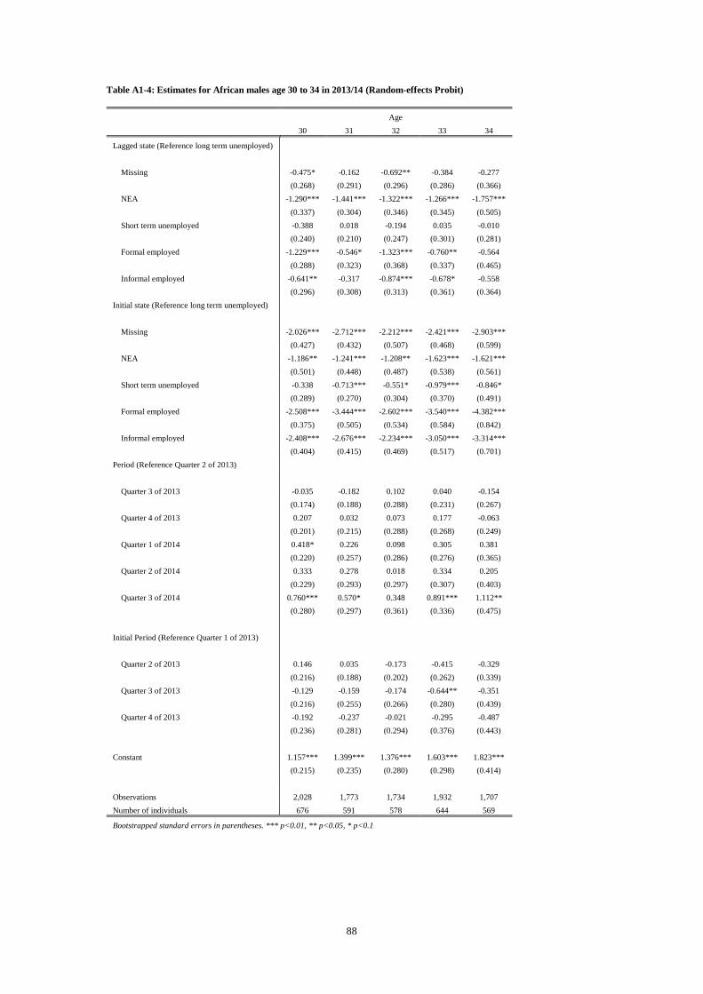
88

Table A1-4: Estimates for African males age 30 to 34 in 2013/14 (Random-effects Probit)

Age

30 31 32 33 34

Lagged state (Reference long term unemployed)

Missing -0.475* -0.162 -0.692** -0.384 -0.277

(0.268) (0.291) (0.296) (0.286) (0.366)

NEA -1.290*** -1.441*** -1.322*** -1.266*** -1.757***

(0.337) (0.304) (0.346) (0.345) (0.505)

Short term unemployed -0.388 0.018 -0.194 0.035 -0.010

(0.240) (0.210) (0.247) (0.301) (0.281)

Formal employed -1.229*** -0.546* -1.323*** -0.760** -0.564

(0.288) (0.323) (0.368) (0.337) (0.465)

Informal employed -0.641** -0.317 -0.874*** -0.678* -0.558

(0.296) (0.308) (0.313) (0.361) (0.364)

Initial state (Reference long term unemployed)

Missing -2.026*** -2.712*** -2.212*** -2.421*** -2.903***

(0.427) (0.432) (0.507) (0.468) (0.599)

NEA -1.186** -1.241*** -1.208** -1.623*** -1.621***

(0.501) (0.448) (0.487) (0.538) (0.561)

Short term unemployed -0.338 -0.713*** -0.551* -0.979*** -0.846*

(0.289) (0.270) (0.304) (0.370) (0.491)

Formal employed -2.508*** -3.444*** -2.602*** -3.540*** -4.382***

(0.375) (0.505) (0.534) (0.584) (0.842)

Informal employed -2.408*** -2.676*** -2.234*** -3.050*** -3.314***

(0.404) (0.415) (0.469) (0.517) (0.701)

Period (Reference Quarter 2 of 2013)

Quarter 3 of 2013 -0.035 -0.182 0.102 0.040 -0.154

(0.174) (0.188) (0.288) (0.231) (0.267)

Quarter 4 of 2013 0.207 0.032 0.073 0.177 -0.063

(0.201) (0.215) (0.288) (0.268) (0.249)

Quarter 1 of 2014 0.418* 0.226 0.098 0.305 0.381

(0.220) (0.257) (0.286) (0.276) (0.365)

Quarter 2 of 2014 0.333 0.278 0.018 0.334 0.205

(0.229) (0.293) (0.297) (0.307) (0.403)

Quarter 3 of 2014 0.760*** 0.570* 0.348 0.891*** 1.112**

(0.280) (0.297) (0.361) (0.336) (0.475)

Initial Period (Reference Quarter 1 of 2013)

Quarter 2 of 2013 0.146 0.035 -0.173 -0.415 -0.329

(0.216) (0.188) (0.202) (0.262) (0.339)

Quarter 3 of 2013 -0.129 -0.159 -0.174 -0.644** -0.351

(0.216) (0.255) (0.266) (0.280) (0.439)

Quarter 4 of 2013 -0.192 -0.237 -0.021 -0.295 -0.487

(0.236) (0.281) (0.294) (0.376) (0.443)

Constant 1.157*** 1.399*** 1.376*** 1.603*** 1.823***

(0.215) (0.235) (0.280) (0.298) (0.414)

Observations 2,028 1,773 1,734 1,932 1,707

Number of individuals 676 591 578 644 569

Bootstrapped standard errors in parentheses. *** p<0.01, ** p<0.05, * p<0.1

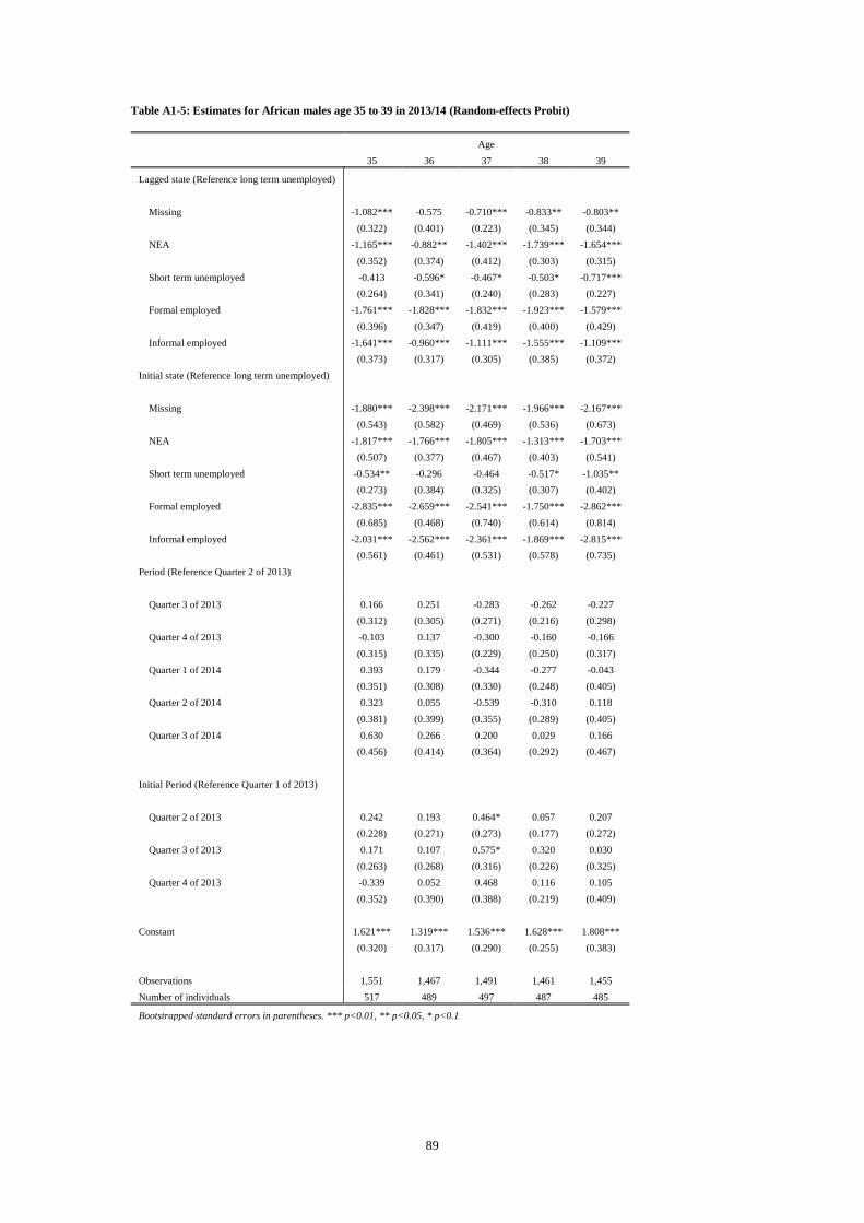
89

Table A1-5: Estimates for African males age 35 to 39 in 2013/14 (Random-effects Probit)

Age

35 36 37 38 39

Lagged state (Reference long term unemployed)

Missing -1.082*** -0.575 -0.710*** -0.833** -0.803**

(0.322) (0.401) (0.223) (0.345) (0.344)

NEA -1.165*** -0.882** -1.402*** -1.739*** -1.654***

(0.352) (0.374) (0.412) (0.303) (0.315)

Short term unemployed -0.413 -0.596* -0.467* -0.503* -0.717***

(0.264) (0.341) (0.240) (0.283) (0.227)

Formal employed -1.761*** -1.828*** -1.832*** -1.923*** -1.579***

(0.396) (0.347) (0.419) (0.400) (0.429)

Informal employed -1.641*** -0.960*** -1.111*** -1.555*** -1.109***

(0.373) (0.317) (0.305) (0.385) (0.372)

Initial state (Reference long term unemployed)

Missing -1.880*** -2.398*** -2.171*** -1.966*** -2.167***

(0.543) (0.582) (0.469) (0.536) (0.673)

NEA -1.817*** -1.766*** -1.805*** -1.313*** -1.703***

(0.507) (0.377) (0.467) (0.403) (0.541)

Short term unemployed -0.534** -0.296 -0.464 -0.517* -1.035**

(0.273) (0.384) (0.325) (0.307) (0.402)

Formal employed -2.835*** -2.659*** -2.541*** -1.750*** -2.862***

(0.685) (0.468) (0.740) (0.614) (0.814)

Informal employed -2.031*** -2.562*** -2.361*** -1.869*** -2.815***

(0.561) (0.461) (0.531) (0.578) (0.735)

Period (Reference Quarter 2 of 2013)

Quarter 3 of 2013 0.166 0.251 -0.283 -0.262 -0.227

(0.312) (0.305) (0.271) (0.216) (0.298)

Quarter 4 of 2013 -0.103 0.137 -0.300 -0.160 -0.166

(0.315) (0.335) (0.229) (0.250) (0.317)

Quarter 1 of 2014 0.393 0.179 -0.344 -0.277 -0.043

(0.351) (0.308) (0.330) (0.248) (0.405)

Quarter 2 of 2014 0.323 0.055 -0.539 -0.310 0.118

(0.381) (0.399) (0.355) (0.289) (0.405)

Quarter 3 of 2014 0.630 0.266 0.200 0.029 0.166

(0.456) (0.414) (0.364) (0.292) (0.467)

Initial Period (Reference Quarter 1 of 2013)

Quarter 2 of 2013 0.242 0.193 0.464* 0.057 0.207

(0.228) (0.271) (0.273) (0.177) (0.272)

Quarter 3 of 2013 0.171 0.107 0.575* 0.320 0.030

(0.263) (0.268) (0.316) (0.226) (0.325)

Quarter 4 of 2013 -0.339 0.052 0.468 0.116 0.105

(0.352) (0.390) (0.388) (0.219) (0.409)

Constant 1.621*** 1.319*** 1.536*** 1.628*** 1.808***

(0.320) (0.317) (0.290) (0.255) (0.383)

Observations 1,551 1,467 1,491 1,461 1,455

Number of individuals 517 489 497 487 485

Bootstrapped standard errors in parentheses. *** p<0.01, ** p<0.05, * p<0.1

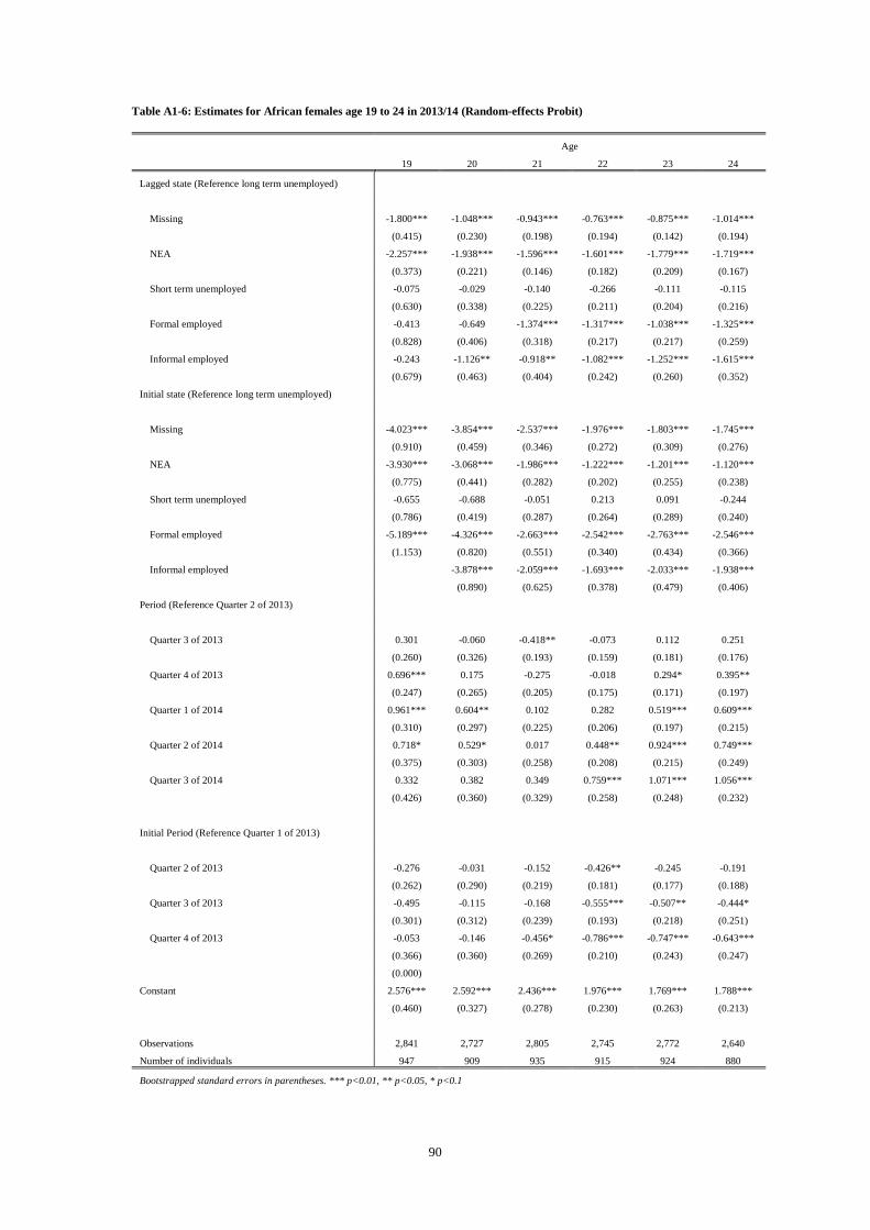
90

Table A1-6: Estimates for African females age 19 to 24 in 2013/14 (Random-effects Probit)

Age

19 20 21 22 23 24

Lagged state (Reference long term unemployed)

Missing -1.800*** -1.048*** -0.943*** -0.763*** -0.875*** -1.014***

(0.415) (0.230) (0.198) (0.194) (0.142) (0.194)

NEA -2.257*** -1.938*** -1.596*** -1.601*** -1.779*** -1.719***

(0.373) (0.221) (0.146) (0.182) (0.209) (0.167)

Short term unemployed -0.075 -0.029 -0.140 -0.266 -0.111 -0.115

(0.630) (0.338) (0.225) (0.211) (0.204) (0.216)

Formal employed -0.413 -0.649 -1.374*** -1.317*** -1.038*** -1.325***

(0.828) (0.406) (0.318) (0.217) (0.217) (0.259)

Informal employed -0.243 -1.126** -0.918** -1.082*** -1.252*** -1.615***

(0.679) (0.463) (0.404) (0.242) (0.260) (0.352)

Initial state (Reference long term unemployed)

Missing -4.023*** -3.854*** -2.537*** -1.976*** -1.803*** -1.745***

(0.910) (0.459) (0.346) (0.272) (0.309) (0.276)

NEA -3.930*** -3.068*** -1.986*** -1.222*** -1.201*** -1.120***

(0.775) (0.441) (0.282) (0.202) (0.255) (0.238)

Short term unemployed -0.655 -0.688 -0.051 0.213 0.091 -0.244

(0.786) (0.419) (0.287) (0.264) (0.289) (0.240)

Formal employed -5.189*** -4.326*** -2.663*** -2.542*** -2.763*** -2.546***

(1.153) (0.820) (0.551) (0.340) (0.434) (0.366)

Informal employed

-3.878*** -2.059*** -1.693*** -2.033*** -1.938***

(0.890) (0.625) (0.378) (0.479) (0.406)

Period (Reference Quarter 2 of 2013)

Quarter 3 of 2013 0.301 -0.060 -0.418** -0.073 0.112 0.251

(0.260) (0.326) (0.193) (0.159) (0.181) (0.176)

Quarter 4 of 2013 0.696*** 0.175 -0.275 -0.018 0.294* 0.395**

(0.247) (0.265) (0.205) (0.175) (0.171) (0.197)

Quarter 1 of 2014 0.961*** 0.604** 0.102 0.282 0.519*** 0.609***

(0.310) (0.297) (0.225) (0.206) (0.197) (0.215)

Quarter 2 of 2014 0.718* 0.529* 0.017 0.448** 0.924*** 0.749***

(0.375) (0.303) (0.258) (0.208) (0.215) (0.249)

Quarter 3 of 2014 0.332 0.382 0.349 0.759*** 1.071*** 1.056***

(0.426) (0.360) (0.329) (0.258) (0.248) (0.232)

Initial Period (Reference Quarter 1 of 2013)

Quarter 2 of 2013 -0.276 -0.031 -0.152 -0.426** -0.245 -0.191

(0.262) (0.290) (0.219) (0.181) (0.177) (0.188)

Quarter 3 of 2013 -0.495 -0.115 -0.168 -0.555*** -0.507** -0.444*

(0.301) (0.312) (0.239) (0.193) (0.218) (0.251)

Quarter 4 of 2013 -0.053 -0.146 -0.456* -0.786*** -0.747*** -0.643***

(0.366) (0.360) (0.269) (0.210) (0.243) (0.247)

(0.000)

Constant 2.576*** 2.592*** 2.436*** 1.976*** 1.769*** 1.788***

(0.460) (0.327) (0.278) (0.230) (0.263) (0.213)

Observations 2,841 2,727 2,805 2,745 2,772 2,640

Number of individuals 947 909 935 915 924 880

Bootstrapped standard errors in parentheses. *** p<0.01, ** p<0.05, * p<0.1

91

Table A1-7: Estimates for African females age 25 to 29 in 2013/14 (Random-effects Probit)

Age

25 26 27 28 29

Lagged state (Reference long term unemployed)

Missing -0.800*** -0.962*** -1.248*** -0.958*** -0.721***

(0.181) (0.146) (0.227) (0.193) (0.174)

NEA -1.359*** -1.288*** -1.702*** -1.626*** -1.645***

(0.155) (0.171) (0.161) (0.170) (0.200)

Short term unemployed -0.185 -0.146 -0.116 0.092 -0.386

(0.222) (0.204) (0.236) (0.246) (0.247)

Formal employed -1.375*** -1.428*** -1.631*** -1.337*** -1.335***

(0.229) (0.232) (0.323) (0.320) (0.256)

Informal employed -1.206*** -1.052*** -0.994*** -0.896*** -1.274***

(0.217) (0.235) (0.218) (0.278) (0.265)

Initial state (Reference long term unemployed)

Missing -2.055*** -1.870*** -1.761*** -2.102*** -2.233***

(0.279) (0.246) (0.332) (0.305) (0.329)

NEA -1.365*** -1.323*** -1.303*** -1.543*** -1.374***

(0.210) (0.261) (0.241) (0.273) (0.280)

Short term unemployed -0.271 -0.381 -0.494 -0.556** -0.162

(0.232) (0.269) (0.314) (0.269) (0.261)

Formal employed -2.428*** -2.702*** -2.739*** -3.239*** -3.279***

(0.341) (0.345) (0.509) (0.431) (0.443)

Informal employed -1.990*** -2.099*** -2.438*** -2.650*** -2.513***

(0.301) (0.359) (0.398) (0.377) (0.407)

Period (Reference Quarter 2 of 2013)

Quarter 3 of 2013 0.041 0.254 0.100 0.093 0.083

(0.201) (0.164) (0.168) (0.215) (0.210)

Quarter 4 of 2013 0.147 0.142 0.010 0.062 0.038

(0.206) (0.164) (0.165) (0.221) (0.194)

Quarter 1 of 2014 0.441** 0.332* 0.153 0.241 0.102

(0.219) (0.180) (0.202) (0.246) (0.225)

Quarter 2 of 2014 0.489** 0.286 0.050 0.212 0.369

(0.238) (0.221) (0.209) (0.284) (0.280)

Quarter 3 of 2014 0.636** 0.432* 0.183 0.268 0.287

(0.292) (0.255) (0.285) (0.296) (0.285)

Initial Period (Reference Quarter 1 of 2013)

Quarter 2 of 2013 -0.087 0.057 -0.087 -0.093 0.158

(0.175) (0.185) (0.164) (0.204) (0.240)

Quarter 3 of 2013 -0.477** -0.013 -0.138 -0.423* -0.285

(0.189) (0.195) (0.180) (0.217) (0.248)

Quarter 4 of 2013 -0.437* 0.064 -0.087 -0.179 -0.120

(0.244) (0.237) (0.193) (0.221) (0.255)

Constant 1.873*** 1.627*** 2.010*** 2.032*** 1.884***

(0.202) (0.175) (0.190) (0.224) (0.222)

Observations 2,703 2,481 2,496 2,553 2,412

Number of individuals 901 827 832 851 804

Bootstrapped standard errors in parentheses. *** p<0.01, ** p<0.05, * p<0.1

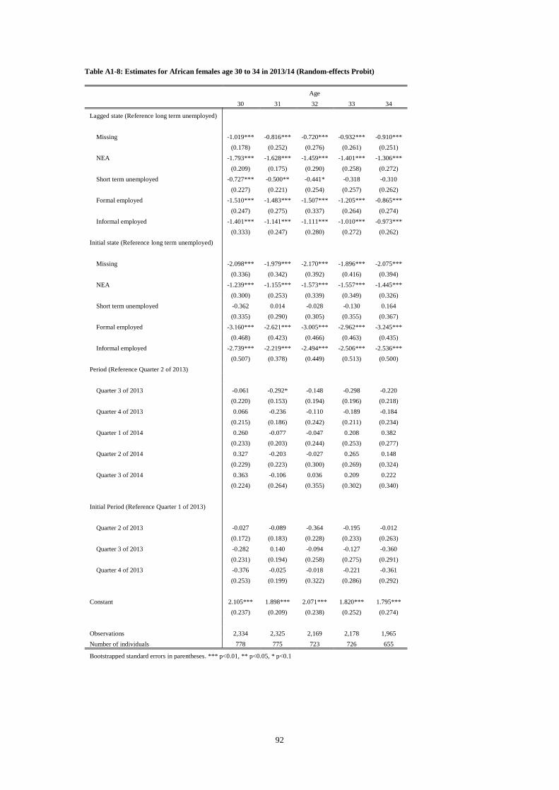
92

Table A1-8: Estimates for African females age 30 to 34 in 2013/14 (Random-effects Probit)

Age

30 31 32 33 34

Lagged state (Reference long term unemployed)

Missing -1.019*** -0.816*** -0.720*** -0.932*** -0.910***

(0.178) (0.252) (0.276) (0.261) (0.251)

NEA -1.793*** -1.628*** -1.459*** -1.401*** -1.306***

(0.209) (0.175) (0.290) (0.258) (0.272)

Short term unemployed -0.727*** -0.500** -0.441* -0.318 -0.310

(0.227) (0.221) (0.254) (0.257) (0.262)

Formal employed -1.510*** -1.483*** -1.507*** -1.205*** -0.865***

(0.247) (0.275) (0.337) (0.264) (0.274)

Informal employed -1.401*** -1.141*** -1.111*** -1.010*** -0.973***

(0.333) (0.247) (0.280) (0.272) (0.262)

Initial state (Reference long term unemployed)

Missing -2.098*** -1.979*** -2.170*** -1.896*** -2.075***

(0.336) (0.342) (0.392) (0.416) (0.394)

NEA -1.239*** -1.155*** -1.573*** -1.557*** -1.445***

(0.300) (0.253) (0.339) (0.349) (0.326)

Short term unemployed -0.362 0.014 -0.028 -0.130 0.164

(0.335) (0.290) (0.305) (0.355) (0.367)

Formal employed -3.160*** -2.621*** -3.005*** -2.962*** -3.245***

(0.468) (0.423) (0.466) (0.463) (0.435)

Informal employed -2.739*** -2.219*** -2.494*** -2.506*** -2.536***

(0.507) (0.378) (0.449) (0.513) (0.500)

Period (Reference Quarter 2 of 2013)

Quarter 3 of 2013 -0.061 -0.292* -0.148 -0.298 -0.220

(0.220) (0.153) (0.194) (0.196) (0.218)

Quarter 4 of 2013 0.066 -0.236 -0.110 -0.189 -0.184

(0.215) (0.186) (0.242) (0.211) (0.234)

Quarter 1 of 2014 0.260 -0.077 -0.047 0.208 0.382

(0.233) (0.203) (0.244) (0.253) (0.277)

Quarter 2 of 2014 0.327 -0.203 -0.027 0.265 0.148

(0.229) (0.223) (0.300) (0.269) (0.324)

Quarter 3 of 2014 0.363 -0.106 0.036 0.209 0.222

(0.224) (0.264) (0.355) (0.302) (0.340)

Initial Period (Reference Quarter 1 of 2013)

Quarter 2 of 2013 -0.027 -0.089 -0.364 -0.195 -0.012

(0.172) (0.183) (0.228) (0.233) (0.263)

Quarter 3 of 2013 -0.282 0.140 -0.094 -0.127 -0.360

(0.231) (0.194) (0.258) (0.275) (0.291)

Quarter 4 of 2013 -0.376 -0.025 -0.018 -0.221 -0.361

(0.253) (0.199) (0.322) (0.286) (0.292)

Constant 2.105*** 1.898*** 2.071*** 1.820*** 1.795***

(0.237) (0.209) (0.238) (0.252) (0.274)

Observations 2,334 2,325 2,169 2,178 1,965

Number of individuals 778 775 723 726 655

Bootstrapped standard errors in parentheses. *** p<0.01, ** p<0.05, * p<0.1

93

Table A1-9: Estimates for African females age 35 to 39 in 2013/14 (Random-effects Probit)

Age

35 36 37 38 39

Lagged state (Reference long term unemployed)

Missing -1.267*** -0.687** -0.557 -0.789** -0.850***

(0.259) (0.325) (0.351) (0.341) (0.329)

NEA -1.566*** -1.583*** -1.710*** -1.790*** -1.627***

(0.205) (0.239) (0.319) (0.281) (0.236)

Short term unemployed -0.538* -0.201 -0.390 -0.399 -0.226

(0.323) (0.317) (0.357) (0.296) (0.320)

Formal employed -1.228*** -1.119*** -1.249*** -1.509*** -1.523***

(0.307) (0.410) (0.391) (0.427) (0.359)

Informal employed -1.314*** -0.656* -0.952*** -1.314*** -1.405***

(0.319) (0.335) (0.313) (0.308) (0.287)

Initial state (Reference long term unemployed)

Missing -1.948*** -2.488*** -3.077*** -2.901*** -2.310***

(0.425) (0.495) (0.696) (0.633) (0.499)

NEA -1.232*** -1.397*** -1.783*** -1.730*** -1.244***

(0.272) (0.345) (0.419) (0.438) (0.257)

Short term unemployed -0.263 -0.895** -0.621 -0.683 -0.493

(0.342) (0.377) (0.434) (0.487) (0.407)

Formal employed -3.298*** -3.699*** -3.714*** -3.915*** -3.413***

(0.463) (0.599) (0.632) (0.731) (0.489)

Informal employed -2.553*** -3.180*** -3.057*** -3.290*** -2.760***

(0.482) (0.505) (0.517) (0.562) (0.512)

Period (Reference Quarter 2 of 2013)

Quarter 3 of 2013 0.078 0.134 -0.070 -0.061 -0.123

(0.250) (0.197) (0.231) (0.229) (0.256)

Quarter 4 of 2013 -0.030 -0.150 -0.188 -0.135 -0.104

(0.253) (0.204) (0.215) (0.242) (0.242)

Quarter 1 of 2014 0.073 -0.093 -0.118 -0.108 -0.111

(0.274) (0.289) (0.255) (0.296) (0.279)

Quarter 2 of 2014 -0.085 -0.085 0.020 0.237 0.091

(0.325) (0.320) (0.286) (0.332) (0.326)

Quarter 3 of 2014 0.001 -0.176 0.151 0.376 -0.147

(0.370) (0.363) (0.347) (0.346) (0.387)

Initial Period (Reference Quarter 1 of 2013)

Quarter 2 of 2013 -0.260 -0.305 -0.112 0.298 0.139

(0.255) (0.216) (0.320) (0.278) (0.279)

Quarter 3 of 2013 0.044 -0.135 -0.149 0.129 -0.269

(0.236) (0.259) (0.328) (0.272) (0.295)

Quarter 4 of 2013 -0.022 -0.128 -0.326 0.199 0.052

(0.265) (0.285) (0.345) (0.265) (0.341)

Constant 2.012*** 2.182*** 2.347*** 2.141*** 1.932***

(0.268) (0.261) (0.328) (0.339) (0.267)

Observations 1,902 1,818 1,890 2,070 1,986

Number of individuals 634 606 630 690 662

Bootstrapped standard errors in parentheses. *** p<0.01, ** p<0.05, * p<0.1

94

This page is intentionally left blank.

95

Chapter 2. Does a targeted wage subsidy voucher have an effect

on the reservation wages of young South Africans?

“The Value or WORTH of a man, is as of all other things, his Price; that is to say, so much as

would be given for the use of his Power...” – T. Hobbes

Abstract

In job search theory the reservation wage of a worker is, ceteris paribus, positively related to

the worker’s probability of receiving wage offers. The reservation wages of young South

Africans may therefore respond to and perhaps even moderate the employment effect of

labour market interventions that improve their probability of receiving wage offers. In this

chapter we use data from a wage subsidy voucher experiment to investigate if the reservation

wages of the beneficiaries in this experiment respond to this employment intervention. We

find that the voucher did not lead to an increase in the reported reservation wages of the

young South Africans in our sample even though the voucher had an employment effect.

However the measures of the reservation wage used in much of the literature in South Africa

are likely to suffer from non-classical measurement error. We show that this measurement

error may be affected by both the survey enumerator and by the phrasing of the questions

used to ascertain the respondent’s reservation wage. Further, we show that the beneficiaries in

our experiment were more likely one year later to be working in jobs where the reported wage

is less than the worker’s reported reservation wage, in jobs where the worker is unhappy with

the job, and they were also more likely to tell us that the pay in these jobs is too low or that

they do not like the job or work environment.

Acknowledgements

I would like to express my gratitude to all the enumerators that worked on the Labour Market

Entry Survey from 2011 to 2012 as well as Kieran De Lange for his assistance.

96

Introduction

A worker’s reservation wage is in principle the lowest wage offer that this worker is willing

to accept for a job. Search theory proposes that it is a function of, among other variables, the

worker’s expectations about the wage offer distribution and the probability of receiving these

offers (Eckstein and Van den Berg, 2007). In this chapter we explore the effect that a targeted

youth wage subsidy voucher has on the reservation wages of young African South Africans.

The wage subsidy voucher could raise the reservation wages of the beneficiaries if they

expect the subsidy to increase the number of offers they receive and (or) the value of any

offers. However the wage subsidy voucher we test is intended to increase employment in the

private sector by reducing the effective wage that a firm has to pay for the worker

(Levinsohn, Rankin, Roberts, and Schöer, 2014). Thus workers’ reservation wages may

moderate the employment-effect of the voucher if it increases their reservation wages as a

result of the subsidy, particularly if these expectations are misinformed. We use data from an

experiment used to assess the impact on employment of a voucher that pays R833 a month for

six months to any formally registered firm that employs the voucher holder. The intervention

was allocated, in 2010, to a randomly selected treatment group from a survey of African

South Africans who were aged 20 to 24 at the time of the first baseline in 2009. Levinsohn et

al. (2014) show the voucher led to an increase in employment among the beneficiaries when

we conducted a follow-up survey in 2011 even though the take-up of the subsidy by firms

was minimal.

The respondents in this experiment were asked “What is the MINIMUM MONTHLY wage

you are prepared to work eight hours a day five days a week for?” We find that that the

voucher did not have a significant effect on the reported reservation wages of the

beneficiaries one year after assignment even though proportionally more of the beneficiaries

were employed. This result corroborates Levinsohn and Pugatch (2014), who estimate a

classical job search model in their “Prospective analysis of a wage subsidy for Cape Town

97

youth” and find that a wage subsidy would increase employment but only lead to a modest

increase in reservation wages. We also find, though, that the voucher appears to have led to a

decrease in the reported reservation wages of the beneficiaries at the time of assignment of

the voucher in 2010. Furthermore the treatment group were significantly more likely, in 2011,

to be employed in jobs where they were earning less than their reported reservation wages.

These results draw our attention to a major shortcoming in the analysis of the effects of

reservation wages on employment in South Africa (and more generally). As Burger, Piraino

and Zoch (2014) point out the reservation wages of young South Africans are likely to be

measured with considerable error. Rankin and Roberts (2011) also find though that many

unemployed youth in South Africa have reservation wages that are higher than what they can

reasonably expect to earn.

One explanation for the difference in the reservation wages in 2010 between the treatment

and control groups is that the value of the voucher served as an anchor for the reported

reservation wages of the treatment group. We also interrogate the measurement errors

associated with the reported reservation wages of youth in South Africa in two ways. First we

randomly allocated the 2011 follow-up surveys to enumerators and we find significant

differences on average in the answers to the reservation wage question based on who the

follow-up surveys are allocated to18. Second we added an open-ended question in 2011 to

determine why those respondents who had initially indicated that their reservation wage (for

work near to where they live) was greater than R1500 also told us that they would be

prepared to accept a job paying R1500? The most common explanations are that the

respondent is “desperate for work”, “not working”, or that the offer is “better than nothing”.

When we then ask the respondents in the experiment sample “IF YOU WERE

COMPLETELY DESPERATE FOR A JOB, what is the MINIMUM MONTHLY wage you

18 We also find differences in the impact of the voucher on employment and reservation wages across this

assignment. However, we are unable to conclude that this is a result of selection because – even though this

assignment was random – we cannot distinguish it from measurement error.

98

are prepared to work eight hours a day five days a week for?” we find that the answer is,

again on average, significantly lower than the reported reservation wage. There is

nevertheless no statistically significant treatment effect, in 2011, on this measure of these

workers’ reservation wages either. Instead we find that the voucher led to a substantial

increase in employment where the worker is either “A bit unhappy” or “Very unhappy” in the

job. We are unable to determine if this is because of the treatment (through e.g. the

expectations that are created), the unobserved characteristics associated with the workers that

transition into employment as a result of the voucher, or the characteristics of the job such as

the wage. This is also why we are unable to determine if the observed decrease in reservation

wages among the treatment group we observe in 2010 mediated the employment effect of the

voucher19 . There is however no difference in the general wellbeing of the young South

Africans in the experiment treatment and control samples one year after the allocation of the

voucher. This suggests that the intervention may not have increased wellbeing within the

experiment population, at least by the noisy measure of wellbeing we use in this paper20.

This chapter proceeds as follows. We briefly outline the literature on reservation wages

among youth in South Africa, present the data from the experiment and the econometric

specifications that we use to explore the effect of the voucher on both the reservation wages

of the sample and job satisfaction among employed workers in this sample, and we then

present the estimates from these models. The chapter ends with a brief discussion.

19 Imai, Keele, Tingley, and Yamamoto (2011) provide an overview of the identifying assumptions we would have

to make. These restrict the analysis of any mediators to exceptional cases.

20 One reason is that, as Posel and Casale (2011) find in South Africa, there may be considerable differences

between objective (such as individual’s ranking in the relevant income distribution) and subjective measures of

wellbeing. Ebrahim, Botha, and Snowball (2013) also find that both employment status and absolute income are

the most important determinants of wellbeing among African South Africans.

99

The reservation wages of young South Africans

Banerjee, Galiani, Levinsohn, McLaren, and Woolard (2008) show that the equilibrium rate

of unemployment in South Africa has been increasing since the end of Apartheid, and argue

that active labour market policies are required to reverse this trend. They arrive at this

conclusion despite finding that it is unlikely unemployment is voluntary, based on evidence

presented by Nattrass and Walker (2005) and Kingdon and Knight (2004). The latter argue

that the most common reason why people are unemployed is because they cannot find any

work, although Banerjee et al. (2008) also discuss evidence by Bertrand et al. (2003) and

Ranchhod (2007) which shows that there is a negative correlation between being employed

and being in a household where some members are recipients of state-funded welfare grants.

More recently Levinsohn and Pugatch (2014) examine the relationship between reservation

wages and unemployment among younger workers in South Africa. They estimate a classical

job search model with data from the Cape Area Panel Survey (CAPS) on the reported

reservation wages of young South Africans21. Their estimates suggest that young workers

implicitly receive many offers that are too low to be accepted. Despite this they also suggest

that an employer wage subsidy would only lead to a moderate increase in reservation wages.

The conclusions they draw from this model are however made under the assumptions that the

firm’s behaviour is exogenous and that workers, once employed, cannot bargain over the

posted wage.

Levinsohn and Pugatch (2014) do not consider institutional features of the labour market such

as minimum wages or union wage-setting since, they argue, the literature in South Africa

suggests that there is low enforcement of minimum wages and only a small proportion of the

respondents in their data reported being union members. Nattrass (2000) and Chandra,

Moorty, Nganou, Rajaratnam, and Schaefer (2001) argue though that the institutional

environment in South Africa has had an effect on employment by increasing the non-wage

21 It is also important to note that the Western Cape is not likely to be representative of the rest of South Africa.

100

cost of labour, and Magruder (2012) finds that centralized bargaining agreements decrease

employment. Further Schultz and Mbawu (1998) believe that a substantial decrease in the

union wage-premium would likely increase employment among African youth. Pauw and

Edwards (2006) note nevertheless that lowering wages in South Africa is a politically

sensitive issue. This is one of the reasons why a wage subsidy is an appealing alternative.

Pauw and Edwards point out that who the wage subsidy is paid to is likely to determine the

outcomes associated with the subsidy. The two designs (employer or employee) are

equivalent only when there are no transaction costs and both the employer and employee have

perfect information (Katz, 1998). Pauw and Edwards (2006: 447) suggest that “when wages

are rigid because of binding minimum wage law, wage subsidies paid to employees are

effective in raising take-home earnings, while employer paid subsidies are more effective in

raising employment.” This will depend on the relative market power of the firms or labour

though. They argue that unions may be able to “counteract the employment generating impact

by negotiating higher wages if the subsidy is paid to the firm, or by prohibiting wage

reductions if the wage is paid to the worker.” Go, Kearney, Korman, Robinson, and

Thierfelder (2010) find that impact of a wage subsidy is likely to be modest if the labour

market is rigid.

Another important constraint to Levinsohn and Pugatch’s (2014) analysis is that they assume

that any measurement error associated with the reported wages that they use to estimate their

model is normally distributed around the true wage and bounded by the respondent’s

reservation wage. They use the median reservation wage for different sub-groups as the input

into their model. Burger, Pariano and Zoch (2014) find though that respondents in South

African labour market surveys may systematically misreport their reservation wages.

Burger et al. (2014) provide an overview of the literature on the measurement of reservation

wages and highlight several reasons why reservation wages are difficult to measure. The first

is that the hypothetical nature of the question, which could lead to “wishful thinking” (Hofler

101

and Murphy, 1994: 962). This is likely to be a problem in South Africa where, as Kingdon

and Knight (2004) point out, the unemployed tend to have limited information about the

labour market. Secondly the characteristics of the job in question are also likely to have an

effect on the wage that the respondent is willing to accept. Groh, McKenzie, Shammout, and

Vishwanath (2014) for example find that reservation prestige is an important factor

underlying the unemployment of educated Jordanian youth. Third, Burger et al. (2014: 1)

show that in South Africa “individuals respond differently when asked whether they would

take up on specific wage offers as compared to reporting the lowest wage they would work

for.” They use the former to construct a more accurate representation of the reservation wage

of youth in South Africa.

Cox and Oaxaca (1992: 1423-1424) argue nevertheless that reservation wages are not

observed in field labour markets because there is no basis for interpreting the answers to

reservation wage questions as corresponding to the theoretical notion of reservation wages in

actual jobs, and that “to induce observable reservation wages, as required for direct tests of

the theory, one needs to conduct experimental trials in which the subject responses consist of

stated minimum acceptable offers for which they are willing to make binding pre-

commitments of acceptance.” They also point out that searchers may use naïve rules in

certain search environments. This is perhaps why Franklin (2014: 5) finds no evidence that a

transport subsidy targeting youth in Ethiopia had an effect on the reservation wages of the job

seekers. Falk, Fehr, and Zender (2006) demonstrate though that economic policy may affect

people's behaviour by shaping their perception of what is a fair and by creating entitlement

effects. They find, using a laboratory experiment, that minimum wages increase subjects’

reservation wages. Importantly this increase persists even after the minimum wage has been

removed. Consequently even if reported reservation wages are not binding they may be

indicative of what individuals believe they are entitled to.

While the assumptions Levinsohn and Pugatch (2014) make in their model do not take into

account some important features of the labour market in South Africa their standard

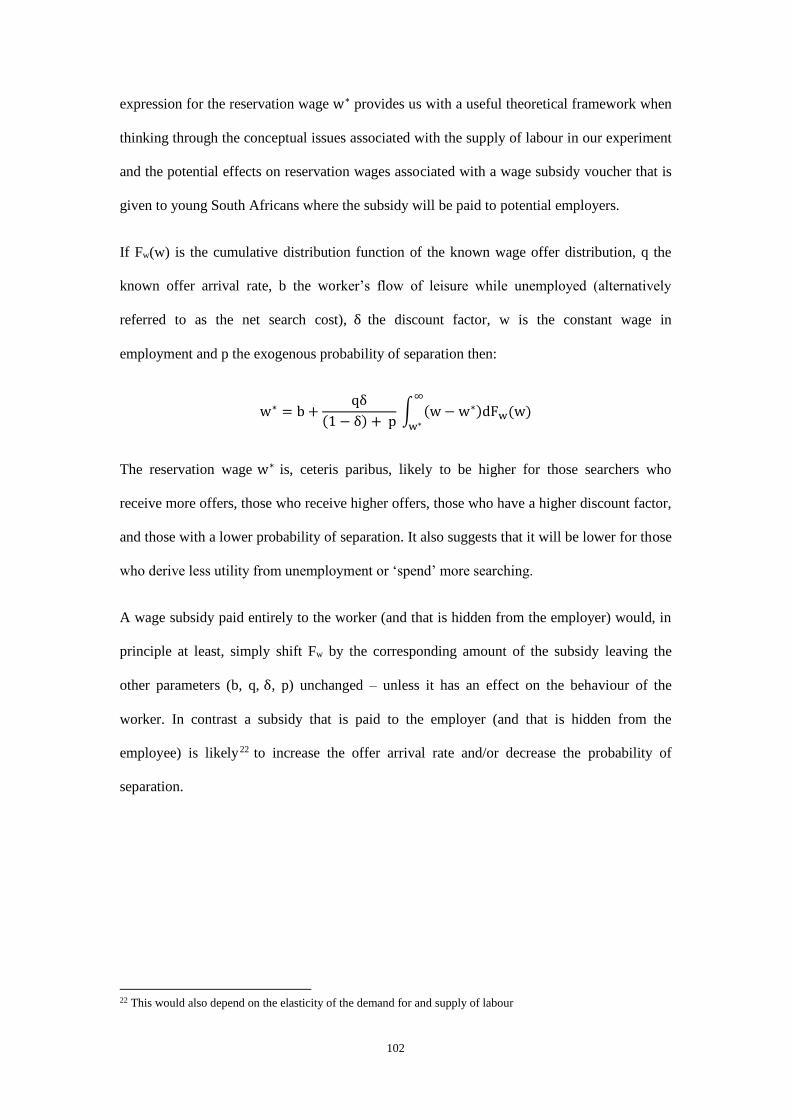
102

expression for the reservation wage w∗ provides us with a useful theoretical framework when

thinking through the conceptual issues associated with the supply of labour in our experiment

and the potential effects on reservation wages associated with a wage subsidy voucher that is

given to young South Africans where the subsidy will be paid to potential employers.

If Fw(w) is the cumulative distribution function of the known wage offer distribution, q the

known offer arrival rate, b the worker’s flow of leisure while unemployed (alternatively

referred to as the net search cost), δ the discount factor, w is the constant wage in

employment and p the exogenous probability of separation then:

w∗ = b +qδ

(1 − δ) + p ∫ (w − w∗)dFw(w)

∞

w∗

The reservation wage w∗ is, ceteris paribus, likely to be higher for those searchers who

receive more offers, those who receive higher offers, those who have a higher discount factor,

and those with a lower probability of separation. It also suggests that it will be lower for those

who derive less utility from unemployment or ‘spend’ more searching.

A wage subsidy paid entirely to the worker (and that is hidden from the employer) would, in

principle at least, simply shift Fw by the corresponding amount of the subsidy leaving the

other parameters (b, q, δ, p) unchanged – unless it has an effect on the behaviour of the

worker. In contrast a subsidy that is paid to the employer (and that is hidden from the

employee) is likely22 to increase the offer arrival rate and/or decrease the probability of

separation.

22 This would also depend on the elasticity of the demand for and supply of labour

103

The data

The respondents in the Labour Market Entry Survey (LMES) which formed the basis for the

wage subsidy voucher experiment were first interviewed in 2009. This sample is drawn from

two sources. The first group (referred to as the EA sub-sample) consisted of individuals that

were interviewed in enumeration areas (EAs) in Johannesburg (Gauteng), Polokwane

(Limpopo), and Durban (KwaZulu-Natal). The second (referred to as the LC sub-sample) was

drawn from young South Africans visiting Department of Labour Labour Centres (LCs) in

these areas at the time the enumerators were at these LCs. The sample locations, while not

representative of South Africa, were chosen to provide the study with variation across

different levels of demand for labour. Gauteng is the economic hub of South Africa,

KwaZulu-Natal the most populous province, and Limpopo has the highest rate of

unemployment in South Africa. The Limpopo Province sample also includes respondents

living in Dikgale which is a semi-rural area.

Rankin, Roberts and Schöer (2015) provide a comprehensive overview of the sampling and

the assignment of the wage subsidy voucher. As mentioned the voucher entitled any formally

registered firm that employed the voucher holder to R833 a month towards the wages of the

beneficiary for six months. The underlying theory of change was that this would encourage

firms to experiment with the worker by reducing some of the cost associated with employing

this worker. The worker would in turn gain work experience and references which could

facilitate continued employment. Rankin et al. (2015: 7) also note that there were transactions

costs associated with the voucher: “In order for a firm to claim the subsidy they needed to

demonstrate that they employed the person with the voucher, through for example a contract,

which was also checked through telephonic contact with the employee. Firms had to be

officially registered for tax and be paying unemployment insurance. To receive the subsidy

payment firms were required to submit a formal invoice to the entity within the university

which managed the project. Payment was made electronically within 30 days of receiving the

invoice. Subsidies were transferable between companies – an individual took the unclaimed

104

subsidy with them should they leave a firm – and for an individual to qualify for a subsidy

they needed to be employed full-time in a formal non-government business”.

The intervention was assigned within gender-location strata using a pair-wise Mahalabonis-

distance (see Mahalanobis, 1936) match based on the datum in 2009 for the respondent’s

education and main labour market activity, and the number of earners in the respondent’s

household. Bruhn and McKenzie (2008) provide an overview of pair-wise matching. In 2010

the respondents were interviewed again and those in the treatment group were, prior to the

interview, told that they were eligible for the subsidy, given the voucher, and a brochure

outlining (to potential employers) how the voucher worked. The brochure text is included in

the Appendix to this chapter (A2-8). While the majority of the respondents were interviewed

in person, those respondents that could not be located in person were interviewed

telephonically. It is important to note that since the voucher was explained before the

interview in 2010 the measures at the time of the interview in 2010 capture the respondents’

responses to the voucher given the information they had about the labour market at that point

(including the offer arrival rate and wage offer distribution).

The respondents were interviewed telephonically in 2011. At the start of the 2011 survey

there were six enumerators working from a call-centre in Johannesburg. The surveys for the

respondents that were interviewed in 2010 for each province were assigned randomly to these

six enumerators in a random order (which we will refer to as the order rank of the assignment

of the surveys in the 2011 LMES). We started with the respondents who we initially sampled

in Gauteng, and then Limpopo and after Limpopo we started calling the respondents from

KwaZulu-Natal (note that some of the respondents may have moved to different provinces

from 2009 to 2010, and from 2010 to 2011). Two enumerators stopped working before the

survey ended and they were replaced by two other enumerators. The treatment respondents

were asked if they understood how the voucher worked, and in those cases where there was a

misunderstanding it was explained to them again (two-thirds of the respondents had

understood the voucher and approximately 54% of the treatment group who were interviewed

105

in 2011 had used the voucher to search for work). All the respondents in the treatment group

were told, again prior to the interview, that the voucher had been extended to 2012. At the end

of the survey the enumerators were asked to go through each other’s lists and interview any of

the respondents that had not already been interviewed (where possible). In 2012 the

respondents were interviewed for a fourth and final time.

In the experiment both the voucher holder and potential employers are aware of the subsidy

and this could have an effect on all of the parameters we outlined earlier in the standard

expression for the reservation wage. Further, it is unlikely that workers will have perfect

information about the wage offer distribution or the offer arrival rate. The role of search costs

is also particularly important in our study because the wage subsidy voucher tested in this

experiment was allocated to randomly selected individuals, both workers and those

individuals that were not in the labour force in 2010. These individuals then had to locate

firms who would be willing to employ them at an effective wage (to the firm) that was at

most R833 less than the worker would be willing to work for since the subsidy would be paid

directly to the employer. The total value of the subsidy was R5000, the voucher-holders

constituted only a small portion of the labour force in the survey locations, and the

respondents were not informed about other workers in the area who had received a voucher23.

It is therefore likely that the impact of the voucher on firms would be at the extensive margin

(i.e. one additional/replacement worker), and that the subsequent wage paid to the worker

would be arrived at through bargaining (even if the accepted wage is the one posted). One of

the benefits of this design24 is that it provides us with insights into the (partial) supply-side

response of the beneficiaries. However it is less informative when assessing the equilibrium

response of firms to such a policy at a larger scale (see e.g. Crépon, Duflo, Gurgand, Rathelot,

and Zamora, 2012). Cartwright (2010) provides an overview of the necessary conditions for

external validity. It is also not clear if the Stable Unit Treatment Value Assumption

23 It was not possible to control this information

24 This design for the RCT was pursued because it corresponded to the proposed policy design at the time.

106

(SUTVA25) holds because the voucher holders may have displaced control respondents in the

queue for jobs. This is why, in this paper, we focus on the effects of the assignment on the

individuals the voucher was assigned to regardless of whether they used the voucher to search

for work.

The following table (Table 2-1) presents the number of observations in the sample. The table

(2-1) shows that there was significant attrition across waves although there is no clear

relationship between this attrition and treatment assignment26. By 2012 almost half of the

original sample attrite. We will confine the analysis to the sample of respondents that were

surveyed in Limpopo and Gauteng because the attrition rates in KwaZulu-Natal significantly

reduce the power of this sub-sample, and this leads to inconclusive inferences (regarding the

effect of the voucher) for most of the outcomes of interest in this province. The Limpopo and

Gauteng samples provide us with (what we believe is) sufficient variation in terms of the

levels of aggregate demand for employment between these two areas (and between

enumerators in 2011) to demonstrate the effect of the voucher, although we also note that the

results do not necessarily reflect the likely outcomes of such a voucher among all young

South Africans.

Table 2-2 presents the number of observations assigned to each enumerator and the number of

observations that were completed by the enumerators within these assignment groups. Table

2-3 presents the number of observations in 2011 by the 2009 baseline characteristics (that

were used to match pairs) of the respondents and that were balanced in 2009.

25 This assumption requires that the treatment assignment in an experiment has no effect on the

outcomes of the respondents in the control group. In our case it would be violated if the respondents in

the control group are less likely to find employment when some of their peers in the treatment group

receive the voucher than they would be if none of the respondents had received the voucher.

26 There are differences within strata, which is one of the reasons we do not use Lee’s (2009) bounds in

the analysis.

107

The selection model (which we will explain in the next section) to correct for non-random

sample attrition will also extend to a small number of respondents that told us in 2011 that

they were not interviewed in 2010 (even though we had collected data on these respondents in

2010). There are several explanations including that the respondent did not remember being

interviewed. Regardless of the reason we will exclude these respondents from the analysis in

2011. There were also a small number of interviews in 2011 where the enumerator indicated

that the respondent was completely or mostly dishonest in the interview and we exclude the

data from these respondents even though we are relying on the perceptions of the

enumerators. Finally there are missing answers to the reported reservation question for some

observations in 2010 and some observations in 2011. Together these limit the sample of 1964

observations in 2011 to a restricted sample of 1761. They also limit the already depleted

sample in 2012 which is why we will not extend the analysis in this paper to 201227. Despite

the restrictions there are no statistically significant differences between the treatment and

control groups in terms of gender, geographical strata, and the 2009 age, education, labour

market state, and the number of earners living in the respondent’s household.

In all of the waves (from 2009 to 2012) the respondents were asked “What is the MINIMUM

MONTHLY wage you are prepared to work eight hours a day five days a week for?” We will

refer to this as the reported reservation wage. They were also asked “What activity currently

takes up most of your time?” and could select only one of the following six answers: “High

27 The surveys were also allocated randomly in the 2012 survey, although they were not assigned to particular

enumerators (we printed a number of pages of surveys to follow up and these were then allocated by the team-

leader to the enumerators once they had completed a page). In future research we hope to explore the longer-term

effects of the voucher on employment on job satisfaction. Our preliminary analysis suggests that the proportion of

treatment respondents in Gauteng who are not unhappy in full-time employment may have increased in 2012 to the

extent that this treatment effect exceeds the equivalent treatment effect for those that are in full-time jobs and

unhappy in these jobs. However, there is no statistically significant effect that can be attributed to the treatment

when we model selection into the 2012 (the treatment group were approximately two percentage-points more

likely to be unhappy in employment) – despite a large treatment effect on employment. This is why we defer the

longer term-effects, and restrict our analysis to the effect of the voucher one year after the assignment.

108

School”, “Further Education”, “Unemployed and NOT searching for work”, “Unemployed

and searching for work”, “Working for someone else” or “Working for yourself”. Table 2-4

presents the levels of unemployment, reservation wages, and employment by treatment status

in 2010 and 2011. The respondents that were “Working for someone else” or “Working for

yourself” were asked how happy they were in the job, and could select one of the following

five responses: “Very happy”, “Reasonably happy”, “Neither happy nor unhappy”, “A bit

unhappy”, or “Very unhappy”.

The following questions were added to the 2011 in the post-treatment follow-up survey: How

do you feel about your life in general (very unhappy, unhappy, okay, happy, and very

happy)?, “What is the MINIMUM MONTHLY wage you are prepared to work eight hours a

day five days a week for NEAR to your home?”, “IF YOU WERE COMPLETELY

DESPERATE FOR A JOB, what is the MINIMUM MONTHLY wage you are prepared to

work eight hours a day five days a week for?”, and “If you were offered a permanent full-time

job near to where you live and that pays R1500 per MONTH for the first year, would you

take it?” Those respondents who indicated that they would accept such a job but who a

reported reservation wage for a job near to they live that was more than R1500 were asked

why they were inconsistent.

In 2011 the employment questions were also extended to those respondents who indicated

that they had worked in the last week prior to the interview even though their main activity

was not “Working for someone else” or “Working for yourself”. We will refer this as any

work (i.e. it includes those respondents that are “Working for someone else” or “Working for

yourself” as their main activity and those respondents in 2011 that did not define their main

activity as “Working for someone else” or “Working for yourself” but had indicated that they

had done some work for someone else or themselves in the past month). We also define those

respondents that did any work for someone else regardless of whether they defined this as

their main activity as having a job. The respondents were also asked to define their self-

reported labour force status and could choose from one of the following six responses:

109

“Employed”, “Unemployed and looking for work”, “Unemployed, I want work but I am not

looking for work”, “Not economically active – still in school”, “Not economically active -

you can't work because you are disabled/ill”, and “Not economically active – you don’t want

to work”.

Table 2-1: Number of observations for each round of the survey, by location strata

Number of observations Proportion treated (%)

Province Strata 2009 2010 2011 2012 2009 2010 2011 2012

Gauteng EA: Alexandra and Hillbrow 228 159 122 84 50 59 57 57

EA: East Rand 174 138 99 66 49 53 53 52

EA: Soweto 773 604 452 329 50 53 53 55

EA: Thembisa and Ivory Park 154 117 90 72 49 55 52 54

LC: Johannesburg Central 121 94 78 59 50 51 53 53

LC: Johannesburg East 294 230 190 147 50 51 52 54

LC: Soweto 182 167 145 109 49 48 47 43

Limpopo EA: Dikgale 214 174 142 106 50 45 44 45

EA: Lebowakgomo 37 31 25 21 49 45 44 52

EA: Makhado 21 14 12 11 48 50 50 45

EA: Seshego 333 262 212 167 50 47 48 52

EA: Thohoyando 32 22 20 16 50 50 50 44

LC: Limpopo Other 237 211 190 146 50 50 49 51

LC: Polokwane 209 202 187 154 50 50 50 50

Total 3,009 2,425 1,964 1,487 50 51 51 52

Table 2-2: Number of observations assigned to each enumerator and the number of observations that were completed by

the enumerators within these assignment groups

Sample Province

Completed by enumerator

Assigned to enumerator Gauteng Limpopo Total

One Two Three Four Five Six Seven Eight Total

One 259 155 414

321 8 0 2 6 0 8 4 349

Two 250 152 402

11 201 1 1 6 0 97 2 319

Three 250 152 402

4 17 267 1 8 0 13 7 317

Four 250 152 402

6 19 0 262 2 0 31 0 320

Five 250 152 402

1 9 0 3 311 0 4 1 329

Six 250 153 403

1 19 0 10 1 288 9 2 330

Total 1,509 916 2,425

344 273 268 279 334 288 162 16 1,964

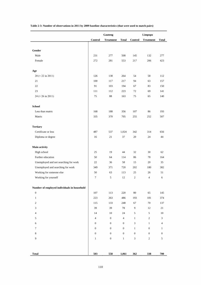
110

Table 2-3: Number of observations in 2011 by 2009 baseline characteristics (that were used to match pairs)

Gauteng Limpopo

Control Treatment Total Control Treatment Total

Gender

Male 231 277 508 145 132 277

Female 272 281 553 217 206 423

Age

20 (≈ 22 in 2011) 126 138 264 54 58 112

21 100 117 217 94 63 157

22 91 103 194 67 83 150

23 111 112 223 72 69 141

24 (≈ 26 in 2011) 75 88 163 75 65 140

School

Less than matric 168 188 356 107 86 193

Matric 335 370 705 255 252 507

Tertiary

Certificate or less 487 537 1,024 342 314 656

Diploma or degree 16 21 37 20 24 44

Main activity

High school 25 19 44 32 30 62

Further education 50 64 114 86 78 164

Unemployed and not searching for work 22 36 58 15 20 35

Unemployed and searching for work 349 371 720 202 180 382

Working for someone else 50 63 113 25 26 51

Working for yourself 7 5 12 2 4 6

Number of employed individuals in household

0 107 113 220 80 65 145

1 223 263 486 193 181 374

2 115 133 248 67 70 137

3 39 39 78 9 12 21

4 14 10 24 5 5 10

5 4 0 4 1 2 3

6 0 0 0 3 1 4

7 0 0 0 1 0 1

8 0 0 0 0 0 0

9 1 0 1 3 2 5

Total 503 558 1,061 362 338 700

111

Table 2-4: Unemployment, reported reservation wages, and employment by treatment status in 2010 and 2011

(Percentage and number of observations)

Unemployed

Reported

reservation

wage

Employed

Employed

but

unhappy in

this

employment

Employed

and not

unhappy in

this

employment

Gauteng

2010

Control 60.04 3632 20.48 7.36 12.92

N 503 503 503 503 503

Treatment 55.91 3478 22.22 9.68 12.54

N 558 558 558 558 558

Total 57.87 3551 21.39 8.58 12.72

1061 1061 1061 1061 1061

2011

Control 45.13 4584 30.62 9.34 21.27

N 503 503 503 503 503

Treatment 37.63 4638 38.71 13.98 24.73

N 558 558 558 558 558

Total 41.19 4613 34.87 11.78 23.09

1061 1061 1061 1061 1061

Limpopo

2010

Control 56.08 3273 16.02 4.70 11.33

N 362 362 362 362 362

Treatment 55.03 3364 16.86 6.21 10.65

N 338 338 338 338 338

Total 55.57 3317 16.43 5.43 11.00

700 700 700 700 700

2011

Control 35.91 3983 29.28 7.18 21.82

N 362 362 362 362 362

Treatment 32.25 3849 33.43 9.17 24.26

N 338 338 338 338 338

Total 34.14 3918 31.29 8.14 23.00

700 700 700 700 700

In Gauteng the reported reservation wages of the treatment group were approximately R 150 less on average than they were for

the control group in 2010, and the treatment group in this province was less likely to be unemployed and more likely to be

employed at the time the voucher was assigned to the beneficiaries when compared to the control group. In 2011 the treatment

groups in both provinces were less likely to be unemployed and more likely to be employed than the control groups in these

provinces. It is unclear if the voucher employment effect is associated with differences in job-satisfaction.

112

The econometric approach

In the following section we estimate the Intention To Treat (ITT) effects of the voucher on

reservation wages using Heckman’s Full Maximum Likelihood Estimator (Heckman, 1979)

for continuous outcomes for selection from 2010 to the restricted sample in 2011:

𝑦𝑖 = 𝑥𝑖⃗⃗⃗⃗ + 𝑢1𝑖 (1)

𝑥𝑖⃗⃗⃗⃗ + 𝑧𝑖⃗⃗ ⃗ + 𝑢2𝑖 > 0

𝑢𝑖1~ 𝑁(0, 𝜎)

𝑢𝑖2~ 𝑁(0,1)

𝑐𝑜𝑟𝑟 (𝑢𝑖1, 𝑢𝑖2) = 𝜌

We use a probit model with sample selection (Van de Ven and Van Pragg 1981) for the

binary labour market outcomes such as unemployment and employment:

𝑦𝑖∗ = 𝑥𝑖⃗⃗⃗⃗ + 𝑢1𝑖 (2)

𝑢𝑖1~ 𝑁(0,1)

The vector 𝑥𝑖⃗⃗⃗⃗ of explanatory variables, for each individual (i), includes:

(𝑡 ∗ 𝑒 ∗ 𝑝) + 𝑔 + �⃗� + 𝑠 + 𝑚 + 𝑑

(𝑡 ∗ 𝑒 ∗ 𝑝) is the full interaction of treatment assignment 𝑡, the enumerator the respondent-

survey was randomly assigned to (initially), 𝑒, and the province (Gauteng or Limpopo) the

respondent was sampled in,

𝑔 is the gender of the respondent?

�⃗� is the age of the respondent in 2009 (a set of dummy variables for ages 20 to 24),

𝑠 is the geographical strata in which the treatment assignment was made (there are twelve),

113

𝑚 indicates if the respondent has a matric, and 𝑑 indicates if the respondent has a degree or

diploma (all in 2009).

The Heckman correction for sample selection requires a set of exclusion restrictions in the

first stage regression that are not included in the second stage regression. These are variables

that are correlated with selection into the sample but not with the outcomes of interest (other

than through the correlation with selection into the sample). Similarly, all the covariates that

are included in the second stage need to be included in the first stage when we model

selection into the sample in 2011, and we cannot add additional covariates in the second state

that are not included in the first stage. The vector 𝑧𝑖⃗⃗ ⃗ of exclusion restrictions for each

individual includes:

(𝑡 ∗ 𝑒 ∗ 𝑝 ∗ 𝑜) + (𝑝 ∗ 𝑑𝑝𝑛) + ( 𝑝 ∗ 𝑙𝑔)

𝑜 is the order rank that the survey was randomly assigned for each enumerator group in the

2011 survey for all the individuals that we interviewed in 2010. In other words it is the order

in which the enumerators would have been presented with prompt sheets for particular

individuals that were interviewed in 2010 and the enumerators would have to interview in

2011.

𝑑𝑝𝑛 is the difference in the number of phone numbers that were collected in 2010 from the

number that were collected in 2009 for the individual that was interviewed prior to the

respondent by the enumerator interviewing the respondent in 2010 (which was, on average,

one additional number).

There is a correlation between the randomly assigned order rank and participation in 2011 for

some of the enumerators (as we show in the Appendix when we present the estimates from

the specification). We attribute this to enumerator fatigue. There is also a correlation between

attrition in 2011 and the number of phone numbers that were captured in 2010, most likely

because the 2011 interviews were conducted telephonically. However the number of phone

numbers for any individual is also likely to be correlated with our outcomes of interest. This

114

is why we use the difference for the individual that was surveyed, by the same enumerator in

2010, prior to the respondent. We set this difference to zero for the first respondent that each

of the 37 enumerators in 2010 interviewed.

𝑙𝑔 is the gender of the respondent that was randomly assigned in an order one rank above (i.e.

prior to) the respondent’s prompt sheet in 2011. We include this variable as an exclusion

restriction because 𝑑𝑝𝑛 is not significant for the respondents from Limpopo28 and we attribute

this relationship to the higher response-rate among females in this province (so that the

enumerator would presumably feel less pressure to interview the subsequent respondent in the

randomly-ordered list of prompt sheets).

We do not include the employment state or number of earners29 at the initial baseline (2009)

in 𝑥𝑖⃗⃗⃗⃗ to avoid using lagged dependent-variables. Achen (2000) explains how lagged

dependent variables may bias the estimates of the other coefficients in a specification. Further

we use a parsimonious specification to avoid introducing any additional correlation between

the assignment to the treatment, attrition, and the error term; and we do not correct for

selection from 2009 to 2010 because this requires additional assumptions about the validity of

all candidate exclusion restrictions. We interact 𝑡 ∗ 𝑒 ∗ 𝑝 in both the outcome and selection

equations to ensure that the error terms for these two models are not correlated because of any

measurement error (although we assume that any measurement error is, conditional on the

enumerator the survey was assigned to, orthogonal to 𝑜).

As we will show in next section the approach to selection on unobservable characteristics that

we use reduces the difference in the levels of employment and unemployment between the

two groups (i.e. treatment and control) in 2010. While the employment outcomes are not

28 Male respondents from Limpopo were more likely to attrite from 2010 to 2011 than their female counterparts

and this may be why, we speculate, the respondents who were interviewed after a male were more likely to be

interviewed in 2011, at least in the Limpopo sample (because the enumerators were paid for every interview they

completed this could have motivated the enumerators to press a subsequent respondent).

29 The number of earners in the household includes the respondent.

115

central to this chapter we present the effect of the voucher on these outcomes to demonstrate

the effect of controlling for selection on unobservables and to demonstrate that the results

correspond to those in Rankin et al. (2015) even though we use a different specification to

estimate the treatment effect. However we nevertheless note that the internal validity of the

estimates we present in the next section may still be sensitive to unobserved differences

between the treatment and control groups. In particular the control group was less likely than

the treatment group to be “Employed but unhappy in this employment” (Table 2-4) when

these respondents were interviewed in 2010. This is a serious concern because the differences

in employment may be due to employed workers in the treatment group who were more likely

to participate in the LMES because they were unhappy in their jobs and believed participating

in the experiment would help them find better jobs. Alternately the respondents in the

treatment group may have been more likely to report that they were unhappy in their jobs

because they believed they would getter jobs by participating in the experiment.

116

Results

We start by estimating the effect of the treatment on unemployment, the reported reservation

wage, and employment. After this we explore the relationship between treatment status and

other outcomes such as alternate measures of employment, job satisfaction, the relationship

between job satisfaction, earnings and reservation wages, and wellbeing.

Henceforth unemployed (both searching and non-searching) and wage-employed refer to the

activity that takes up most of the respondent’s time. In Table 2-5 we present the results of

three separate estimates for each of the outcomes of interest (we present these results when

we estimate the specifications separately for Gauteng and Limpopo in Table A2-1 and for

each of the six enumerators in Table A2-2 to Table A2-4 in the Appendix to this chapter). The

first is for the model where we do not impose any restrictions on the sample. In 2010 this

includes all 2425 respondents that were interviewed in Gauteng and Limpopo, unless the data

for the outcome is missing. In 2011 this refers to all of the 1964 observations. We then

present the estimates of the restricted sample without any selection correction. The restricted

sample refers to the 1761 respondents that we observe in both 2010 and 2011 and have not

dropped because of concerns about the quality of the data. Finally we present the estimates

for this restricted sample when we include the selection correction.

Table A2-5, Table A2-6, and Table A2-7 in the Appendix present the regression estimates for

unemployment, reservation wages and employment. These tables show that the exclusion

restrictions we use are correlated with selection into the sample. Table 2-5 presents both the

predicted level of the outcome for the control and treatment groups, and the difference

between the levels of the outcome – which we call the Intention To Treat effect (ITT). The

Intention To Treat measures the effect of the assignment on outcomes, regardless of whether

the individuals that were assigned to the treatment group used the voucher. It therefore

measures the causal effect of the assignment and not necessarily the effect of the treatment

(which in our case would be defined as using the voucher when searching for work). The

117

predictions for the probit models are the Average Marginal Effects at the observed values of

the sample. For the third set of regressions – where we include the selection correction – the

Average Marginal Effect is calculated across both the restricted sample and the observations

that we observe in 2010 (even though the outcome equation is estimated using only the 1761

observations in the restricted sample). The standard error of the ITT is displayed in

parenthesis adjacent to the treatment effect.

The selection correction reduces the differences in the level of unemployment and wage-

employment between the treated and control groups in 2010. However the significant

negative relationship between reported reservation wages and assignment to the voucher

persists. There are several explanations. One is that the voucher may have served as an anchor

on the respondents reported reservation wages. Another is that at least some of the voucher-

holders misunderstood the voucher. In 2010 all the respondents who received the voucher

were asked “Do you think the subsidy will make it easier for you to find a job?” and “Why do

you think the subsidy will/will not make it easier for you to find a job”. The opened-ended

answers have been coded into groups. Similarly the respondents in 2011 were asked to

explain how the voucher worked and these answers have also been coded into groups. The

coded responses are presented in Table A2-9 and Table A2-10. It appears that some of the

respondents may have believed that the subsidy would be paid to them. Others appeared to

believe that it was an endorsement from the University of the Witwatersrand. When we

explore the effect of these interpretations we find no descriptive evidence to support the

explanation that any particular misunderstanding led to the differences in the reservation

wages of the treatment group in 2010. Even those respondents who suggested that the subsidy

would benefit, or get paid to, the firm employing the respondent had lower reported

reservation wages than their matched-pair counterparts in the control group.

A second explanation is that this is due to measurement error. In 2010 the enumerators were

not randomly assigned to surveys. This makes it difficult to determine if these differences can

be attributed to the enumerators who interviewed the treatment respondents (or, conversely,

118

those who interviewed the control respondents). We cannot for example follow Allcott and

Mullainathan’s (2012) proposed test for treatment heterogeneity (because the treatment and

control groups are not balanced across enumerators in 201030). As mentioned we only started

randomly assigning surveys to enumerators in 2011. Although there was some contamination,

the six assignment groups in 2011 provide us with an opportunity to explore the potential

effects that the enumerators may have had on reported reservation wages. We did not check

for balance when we assigned these surveys though and so there are a few minor – but

statistically significant – differences in the baselines characteristics across these assignment

groups.

We find that for at least some of these groups there are significant differences in the reported

reservation wages that can be attributed to the enumerator31. For example, Table A2-6 and

Figure A2-1 in the Appendix to this chapter show that the respondents that were assigned to

enumerator six had reported reservation wages in 2011 that were lower on average by as

much as 60% when compared to those that were assigned to the other enumerators. There are

a number of potential explanations for this discrepancy. Regardless, the potential effect of the

enumerator in 2010 makes it difficult conclude that the voucher lowered the reservation-

wages of the beneficiaries in the 2010 round of the LMES. The random assignment of

enumerators in 2011 should reduce any potential bias in the third round of the survey. We

were surprised however to find that the treatment assignment did not have a significant effect

on the reservation wages of the treatment group even though they were significantly more

likely to be employed in 2011 and, presumably, more employable32. We also find that there is

no treatment effect for the question “If you were offered a permanent full-time job near to

where you live and that pays R1500 per MONTH for the first year, would you take it?” We

30 Another approach would be to use propensity score matching (PSM). However there is very little common

support because the enumerators were generally assigned to specific enumeration areas (by treatment status).

31 Table A-2, Table A-3 and Table A-4 in the Appendix present the treatment effect for each enumerator-group.

32 If we assume that employment experience leads to the accumulation of skills and future employment.

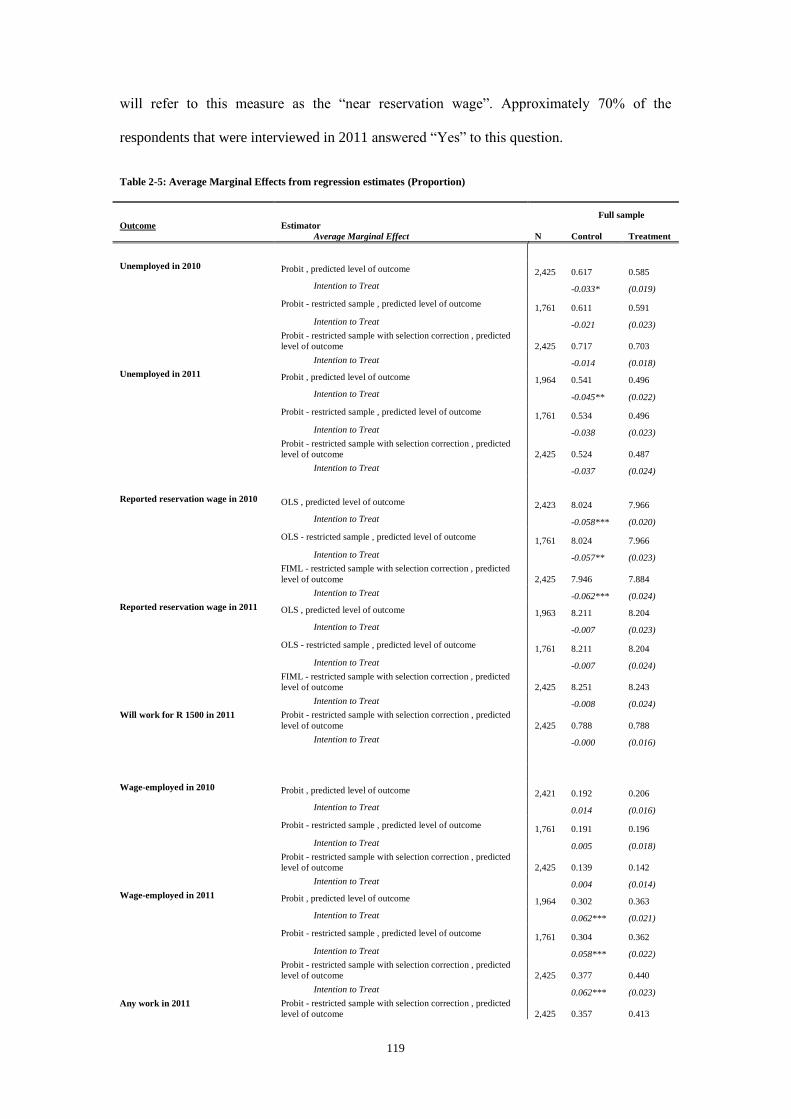
119

will refer to this measure as the “near reservation wage”. Approximately 70% of the

respondents that were interviewed in 2011 answered “Yes” to this question.

Table 2-5: Average Marginal Effects from regression estimates (Proportion)

Full sample

Outcome Estimator

Average Marginal Effect N Control Treatment

Unemployed in 2010 Probit , predicted level of outcome 2,425 0.617 0.585

Intention to Treat

-0.033* (0.019)

Probit - restricted sample , predicted level of outcome 1,761 0.611 0.591

Intention to Treat

-0.021 (0.023)

Probit - restricted sample with selection correction , predicted

level of outcome 2,425 0.717 0.703

Intention to Treat

-0.014 (0.018)

Unemployed in 2011 Probit , predicted level of outcome 1,964 0.541 0.496

Intention to Treat

-0.045** (0.022)

Probit - restricted sample , predicted level of outcome 1,761 0.534 0.496

Intention to Treat

-0.038 (0.023)

Probit - restricted sample with selection correction , predicted

level of outcome 2,425 0.524 0.487

Intention to Treat

-0.037 (0.024)

Reported reservation wage in 2010 OLS , predicted level of outcome 2,423 8.024 7.966

Intention to Treat

-0.058*** (0.020)

OLS - restricted sample , predicted level of outcome 1,761 8.024 7.966

Intention to Treat

-0.057** (0.023)

FIML - restricted sample with selection correction , predicted

level of outcome 2,425 7.946 7.884

Intention to Treat

-0.062*** (0.024)

Reported reservation wage in 2011 OLS , predicted level of outcome 1,963 8.211 8.204

Intention to Treat

-0.007 (0.023)

OLS - restricted sample , predicted level of outcome 1,761 8.211 8.204

Intention to Treat

-0.007 (0.024)

FIML - restricted sample with selection correction , predicted

level of outcome 2,425 8.251 8.243

Intention to Treat

-0.008 (0.024)

Will work for R 1500 in 2011 Probit - restricted sample with selection correction , predicted

level of outcome 2,425 0.788 0.788

Intention to Treat

-0.000 (0.016)

Wage-employed in 2010 Probit , predicted level of outcome 2,421 0.192 0.206

Intention to Treat

0.014 (0.016)

Probit - restricted sample , predicted level of outcome 1,761 0.191 0.196

Intention to Treat

0.005 (0.018)

Probit - restricted sample with selection correction , predicted

level of outcome 2,425 0.139 0.142

Intention to Treat

0.004 (0.014)

Wage-employed in 2011 Probit , predicted level of outcome 1,964 0.302 0.363

Intention to Treat

0.062*** (0.021)

Probit - restricted sample , predicted level of outcome 1,761 0.304 0.362

Intention to Treat

0.058*** (0.022)

Probit - restricted sample with selection correction , predicted

level of outcome 2,425 0.377 0.440

Intention to Treat

0.062*** (0.023)

Any work in 2011 Probit - restricted sample with selection correction , predicted

level of outcome 2,425 0.357 0.413

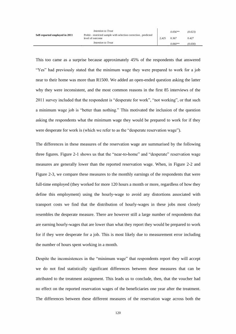
120

Intention to Treat

0.056** (0.023)

Self-reported employed in 2011 Probit - restricted sample with selection correction , predicted

level of outcome 2,425 0.367 0.427

Intention to Treat 0.060** (0.030)

This too came as a surprise because approximately 45% of the respondents that answered

“Yes” had previously stated that the minimum wage they were prepared to work for a job

near to their home was more than R1500. We added an open-ended question asking the latter

why they were inconsistent, and the most common reasons in the first 85 interviews of the

2011 survey included that the respondent is “desperate for work”, “not working”, or that such

a minimum wage job is “better than nothing.” This motivated the inclusion of the question

asking the respondents what the minimum wage they would be prepared to work for if they

were desperate for work is (which we refer to as the “desperate reservation wage”).

The differences in these measures of the reservation wage are summarised by the following

three figures. Figure 2-1 shows us that the “near-to-home” and “desperate” reservation wage

measures are generally lower than the reported reservation wage. When, in Figure 2-2 and

Figure 2-3, we compare these measures to the monthly earnings of the respondents that were

full-time employed (they worked for more 120 hours a month or more, regardless of how they

define this employment) using the hourly-wage to avoid any distortions associated with

transport costs we find that the distribution of hourly-wages in these jobs most closely

resembles the desperate measure. There are however still a large number of respondents that

are earning hourly-wages that are lower than what they report they would be prepared to work

for if they were desperate for a job. This is most likely due to measurement error including

the number of hours spent working in a month.

Despite the inconsistences in the “minimum wage” that respondents report they will accept

we do not find statistically significant differences between these measures that can be

attributed to the treatment assignment. This leads us to conclude, then, that the voucher had

no effect on the reported reservation wages of the beneficiaries one year after the treatment.

The differences between these different measures of the reservation wage across both the

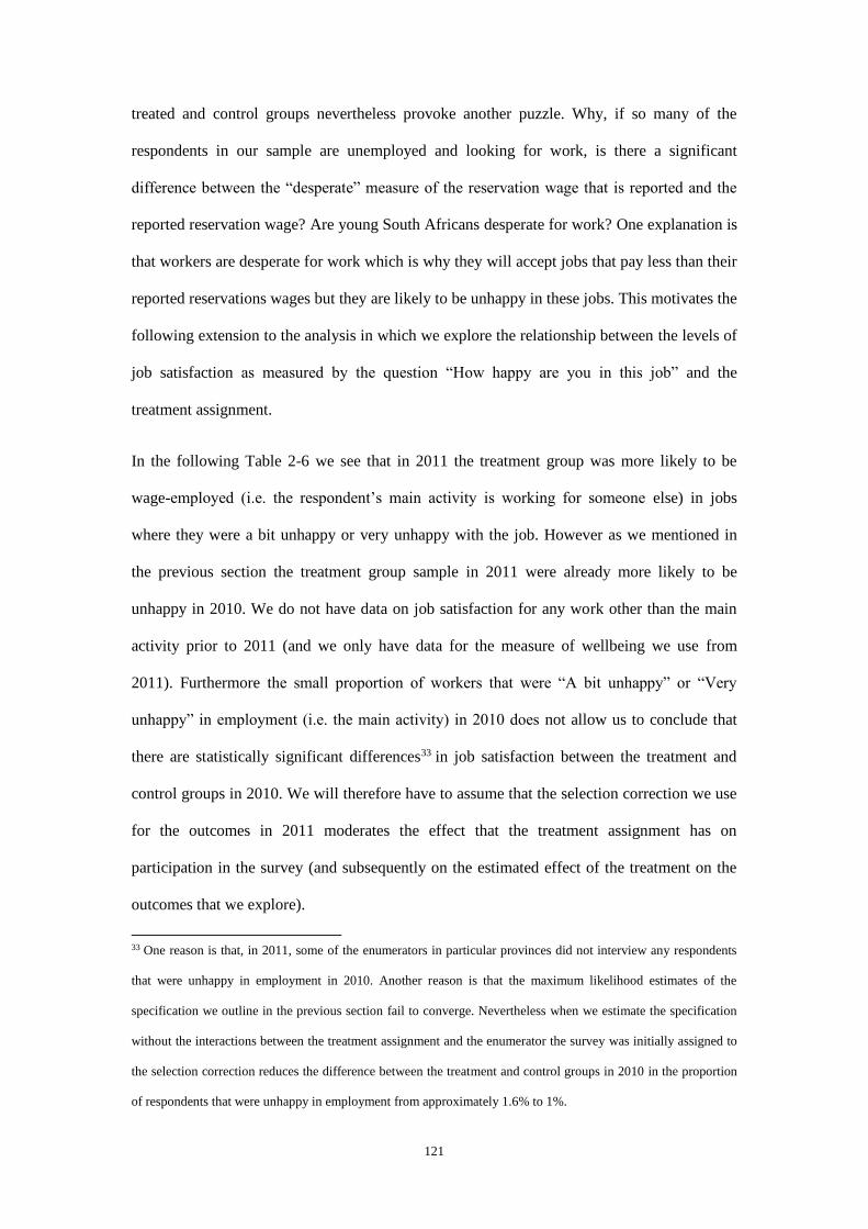
121

treated and control groups nevertheless provoke another puzzle. Why, if so many of the

respondents in our sample are unemployed and looking for work, is there a significant

difference between the “desperate” measure of the reservation wage that is reported and the

reported reservation wage? Are young South Africans desperate for work? One explanation is

that workers are desperate for work which is why they will accept jobs that pay less than their

reported reservations wages but they are likely to be unhappy in these jobs. This motivates the

following extension to the analysis in which we explore the relationship between the levels of

job satisfaction as measured by the question “How happy are you in this job” and the

treatment assignment.

In the following Table 2-6 we see that in 2011 the treatment group was more likely to be

wage-employed (i.e. the respondent’s main activity is working for someone else) in jobs

where they were a bit unhappy or very unhappy with the job. However as we mentioned in

the previous section the treatment group sample in 2011 were already more likely to be

unhappy in 2010. We do not have data on job satisfaction for any work other than the main

activity prior to 2011 (and we only have data for the measure of wellbeing we use from

2011). Furthermore the small proportion of workers that were “A bit unhappy” or “Very

unhappy” in employment (i.e. the main activity) in 2010 does not allow us to conclude that

there are statistically significant differences33 in job satisfaction between the treatment and

control groups in 2010. We will therefore have to assume that the selection correction we use

for the outcomes in 2011 moderates the effect that the treatment assignment has on

participation in the survey (and subsequently on the estimated effect of the treatment on the

outcomes that we explore).

33 One reason is that, in 2011, some of the enumerators in particular provinces did not interview any respondents

that were unhappy in employment in 2010. Another reason is that the maximum likelihood estimates of the

specification we outline in the previous section fail to converge. Nevertheless when we estimate the specification

without the interactions between the treatment assignment and the enumerator the survey was initially assigned to

the selection correction reduces the difference between the treatment and control groups in 2010 in the proportion

of respondents that were unhappy in employment from approximately 1.6% to 1%.

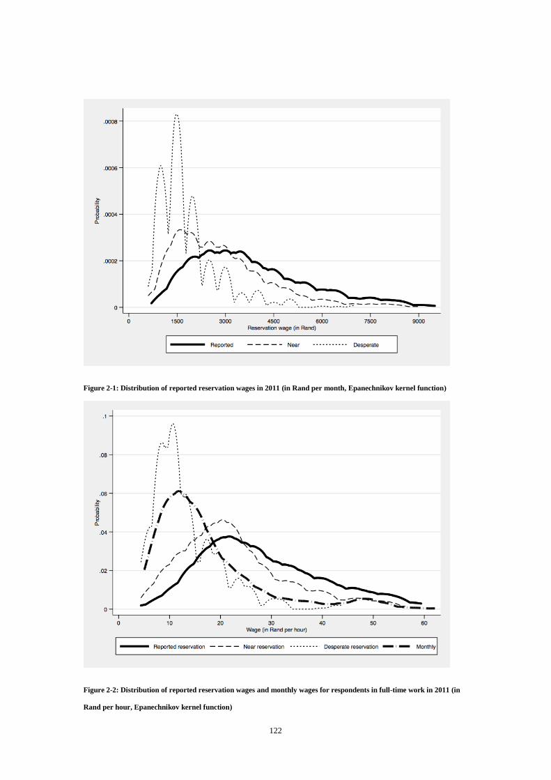
122

Figure 2-1: Distribution of reported reservation wages in 2011 (in Rand per month, Epanechnikov kernel function)

Figure 2-2: Distribution of reported reservation wages and monthly wages for respondents in full-time work in 2011 (in

Rand per hour, Epanechnikov kernel function)

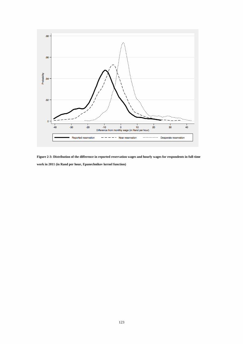
123

Figure 2-3: Distribution of the difference in reported reservation wages and hourly wages for respondents in full-time

work in 2011 (in Rand per hour, Epanechnikov kernel function)

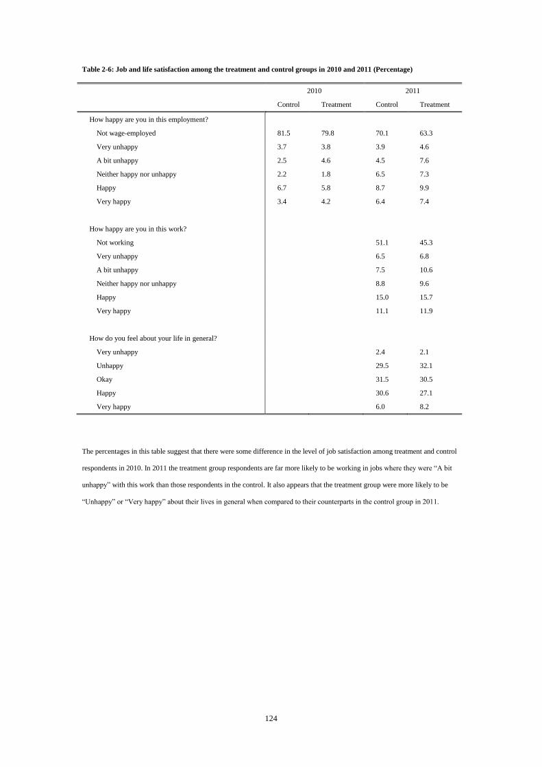
124

Table 2-6: Job and life satisfaction among the treatment and control groups in 2010 and 2011 (Percentage)

2010 2011

Control Treatment Control Treatment

How happy are you in this employment?

Not wage-employed 81.5 79.8 70.1 63.3

Very unhappy 3.7 3.8 3.9 4.6

A bit unhappy 2.5 4.6 4.5 7.6

Neither happy nor unhappy 2.2 1.8 6.5 7.3

Happy 6.7 5.8 8.7 9.9

Very happy 3.4 4.2 6.4 7.4

How happy are you in this work?

Not working

51.1 45.3

Very unhappy

6.5 6.8

A bit unhappy

7.5 10.6

Neither happy nor unhappy

8.8 9.6

Happy

15.0 15.7

Very happy

11.1 11.9

How do you feel about your life in general?

Very unhappy

2.4 2.1

Unhappy

29.5 32.1

Okay

31.5 30.5

Happy

30.6 27.1

Very happy

6.0 8.2

The percentages in this table suggest that there were some difference in the level of job satisfaction among treatment and control

respondents in 2010. In 2011 the treatment group respondents are far more likely to be working in jobs where they were “A bit

unhappy” with this work than those respondents in the control. It also appears that the treatment group were more likely to be

“Unhappy” or “Very happy” about their lives in general when compared to their counterparts in the control group in 2011.

125

We define the binary variable for being unhappy (very unhappy or a bit unhappy) in

employment as one, and zero other otherwise (regardless of whether respondent is employed

or not). Conversely, we define not being unhappy in wage-employment as one for those that

are not unhappy and employed, and zero otherwise. Table 2-7 shows us that the voucher-

population was significantly more likely to be employed in 2011 but unhappy in this

employment – even though the difference between their earnings and reservation wage in

2011 was lower than for the counterparts in the control group. This is perhaps why we find

there are no differences in the level of unhappiness, in general, between these two samples in

201134.

We also find, as we show in Table 2-8, that the individuals in the treatment group were

significantly more likely to be in full-time jobs where they were earning less per hour than

their reported reservation wage (hourly) – both in 2011 and in 2011 when we use their

reservation wage in 2010 as the reference (we also show that in 2011 the difference between

the earnings and reported reservation wages of the beneficiaries was larger, on average, than

for the control group). The estimates indicate that most of the difference in these proportions

is associated with being unhappy with this full-time job, although the sample does not have

sufficient power to allow us to conclude that this is the case for the experiment population.

When we explore this outcome over the two sample provinces (presented in Table A2-1 in the

Appendix) though we find a statistically significant treatment effect for being unhappy with

this full-time job in Gauteng and no difference in the proportion of respondents between the

treatment and control groups that were not unhappy in full-time jobs in which they were

earning less than their reported reservation wage in 2011. However when we disaggregate

these two provinces we also find the voucher only had an effect on employment in Gauteng.

This is not surprising because there is as we mentioned earlier significantly more demand for

labour in Gauteng than there is in Limpopo and only 10% of the Limpopo sample that were

interviewed in 2011 had relocated to Gauteng. We also find that the effect of the voucher on

34 Another reason is that this measure of unhappiness is rather blunt.

126

being unhappy in a job earning less than the reported reservation wage in 2011 is larger than

the treatment effect of just being in a job earning less than the reported reservation wage in

this year (the predicted levels are also larger and do not sum although this may be due to the

selection correction).

There are several other constraints to the inferences we are able to draw from the preceding

analysis. First the voucher may merely have altered the distribution of wellbeing, job

satisfaction, reservation wages and/or employment within the treatment population (so that

for example those beneficiaries that would have been employed regardless of the voucher are

less happy with the job perhaps because they expected the voucher to get them a better jobs

etc.). A second limitation is that we don’t know what caused the increase in wage-

employment and if how the respondents interpreted the voucher may have had an effect on

their outcomes. The most likely explanation is that the voucher moved those in the treatment

up the queue for jobs in Gauteng perhaps because it motivated the respondents in some way,

it activated dormant networks or because the association with the project provided the

beneficiaries with more credibility and/or other signalling devices35. Indeed we also find that

the treatment group respondents were more likely to be employed in jobs where they walk to

work. Finally the most concerning explanation for the results we have presented in this

section is that the voucher assignment may have had an effect on the responses of the

respondents in the treatment group. For example the treated workers may have been more

motivated to engage with the survey.

In summary we unable to determine if the outcomes we have presented in this section are

mediated by the treatment assignment alone (through, for example, the expectations that are

created36), the unobserved characteristics associated with the workers that transition into

35 It is interesting to note that we find no difference, in 2011, between the proportion of the treatment and control

groups that have never been employed.

36 The assignment to the treatment appears to have significantly increased the beneficiaries reported expectations

of finding employment in 2010, although the question was dropped from the telephonic survey that was conducted

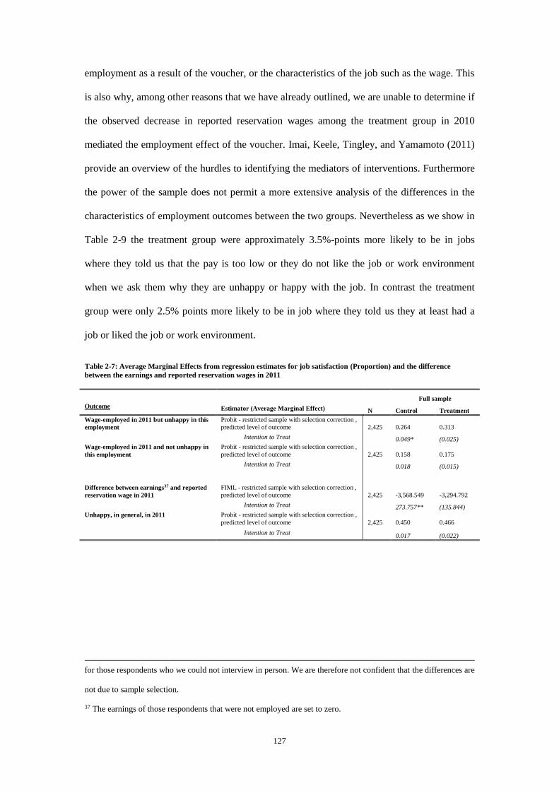
127

employment as a result of the voucher, or the characteristics of the job such as the wage. This

is also why, among other reasons that we have already outlined, we are unable to determine if

the observed decrease in reported reservation wages among the treatment group in 2010

mediated the employment effect of the voucher. Imai, Keele, Tingley, and Yamamoto (2011)

provide an overview of the hurdles to identifying the mediators of interventions. Furthermore

the power of the sample does not permit a more extensive analysis of the differences in the

characteristics of employment outcomes between the two groups. Nevertheless as we show in

Table 2-9 the treatment group were approximately 3.5%-points more likely to be in jobs

where they told us that the pay is too low or they do not like the job or work environment

when we ask them why they are unhappy or happy with the job. In contrast the treatment

group were only 2.5% points more likely to be in job where they told us they at least had a

job or liked the job or work environment.

Table 2-7: Average Marginal Effects from regression estimates for job satisfaction (Proportion) and the difference

between the earnings and reported reservation wages in 2011

Full sample

Outcome Estimator (Average Marginal Effect) N Control Treatment

Wage-employed in 2011 but unhappy in this

employment

Probit - restricted sample with selection correction ,

predicted level of outcome 2,425 0.264 0.313

Intention to Treat

0.049* (0.025)

Wage-employed in 2011 and not unhappy in

this employment

Probit - restricted sample with selection correction ,

predicted level of outcome 2,425 0.158 0.175

Intention to Treat

0.018 (0.015)

Difference between earnings37 and reported

reservation wage in 2011

FIML - restricted sample with selection correction ,

predicted level of outcome 2,425 -3,568.549 -3,294.792

Intention to Treat

273.757** (135.844)

Unhappy, in general, in 2011 Probit - restricted sample with selection correction ,

predicted level of outcome 2,425 0.450 0.466

Intention to Treat

0.017 (0.022)

for those respondents who we could not interview in person. We are therefore not confident that the differences are

not due to sample selection.

37 The earnings of those respondents that were not employed are set to zero.

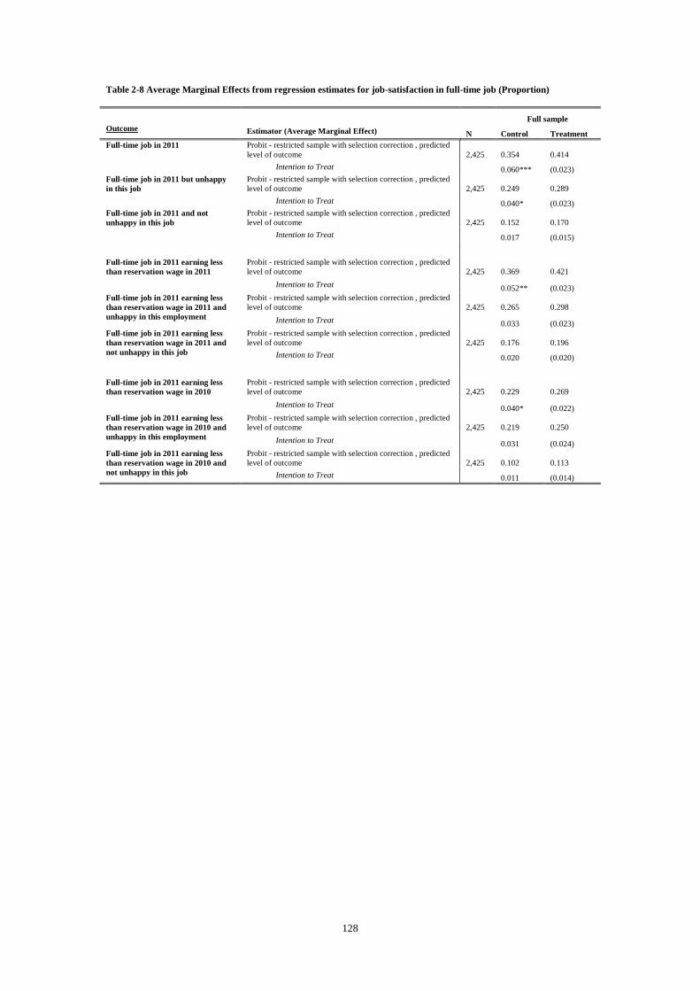
128

Table 2-8 Average Marginal Effects from regression estimates for job-satisfaction in full-time job (Proportion)

Full sample

Outcome Estimator (Average Marginal Effect) N Control Treatment

Full-time job in 2011 Probit - restricted sample with selection correction , predicted

level of outcome 2,425 0.354 0.414

Intention to Treat

0.060*** (0.023)

Full-time job in 2011 but unhappy

in this job

Probit - restricted sample with selection correction , predicted

level of outcome 2,425 0.249 0.289

Intention to Treat

0.040* (0.023)

Full-time job in 2011 and not

unhappy in this job

Probit - restricted sample with selection correction , predicted

level of outcome 2,425 0.152 0.170

Intention to Treat

0.017 (0.015)

Full-time job in 2011 earning less

than reservation wage in 2011

Probit - restricted sample with selection correction , predicted

level of outcome 2,425 0.369 0.421

Intention to Treat

0.052** (0.023)

Full-time job in 2011 earning less

than reservation wage in 2011 and

unhappy in this employment

Probit - restricted sample with selection correction , predicted

level of outcome 2,425 0.265 0.298

Intention to Treat

0.033 (0.023)

Full-time job in 2011 earning less

than reservation wage in 2011 and

not unhappy in this job

Probit - restricted sample with selection correction , predicted

level of outcome 2,425 0.176 0.196

Intention to Treat

0.020 (0.020)

Full-time job in 2011 earning less

than reservation wage in 2010

Probit - restricted sample with selection correction , predicted

level of outcome 2,425 0.229 0.269

Intention to Treat

0.040* (0.022)

Full-time job in 2011 earning less

than reservation wage in 2010 and

unhappy in this employment

Probit - restricted sample with selection correction , predicted

level of outcome 2,425 0.219 0.250

Intention to Treat

0.031 (0.024)

Full-time job in 2011 earning less

than reservation wage in 2010 and

not unhappy in this job

Probit - restricted sample with selection correction , predicted

level of outcome 2,425 0.102 0.113

Intention to Treat

0.011 (0.014)

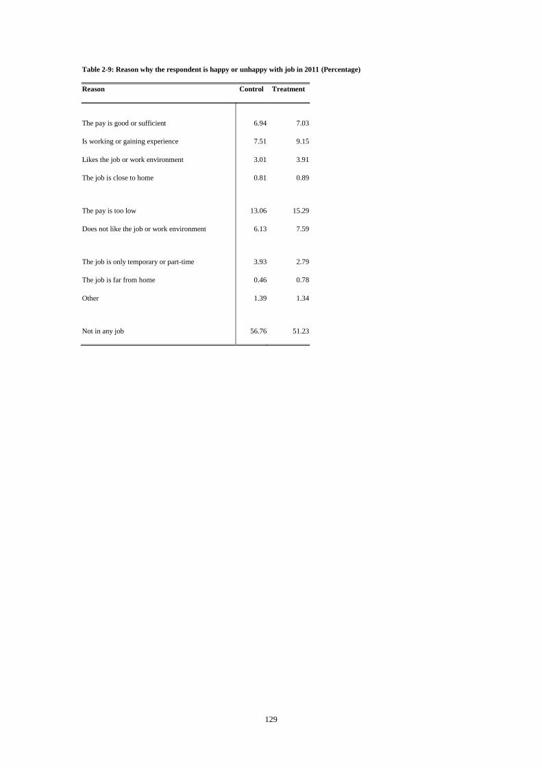
129

Table 2-9: Reason why the respondent is happy or unhappy with job in 2011 (Percentage)

Reason Control Treatment

The pay is good or sufficient 6.94 7.03

Is working or gaining experience 7.51 9.15

Likes the job or work environment 3.01 3.91

The job is close to home 0.81 0.89

The pay is too low 13.06 15.29

Does not like the job or work environment 6.13 7.59

The job is only temporary or part-time 3.93 2.79

The job is far from home 0.46 0.78

Other 1.39 1.34

Not in any job 56.76 51.23

130

Discussion and conclusion

We find using experimental evidence that a wage subsidy voucher has no effect on the

reservation wages of a group of young African South Africans one year after assignment. In

the previous section we noted though that there are several threats to the internal validity of

our estimates of the effect that the wage subsidy voucher had on beneficiaries and the

inferences we can draw from these estimates. We also noted that the sample we use is not

representative of all young people in South Africa. Nevertheless we believe the results that

we have presented support several important conclusions that may contribute to the literature

on youth unemployment in South Africa.

The first is that many measures of the reported reservation wages for South African youth

may suffer from systematic measurement error, and these errors are likely to compromise the

inferences we draw from studies that explore the relationship between reservation wages and

employment outcomes. In particular there are significant differences in the reported

reservation wages and the other measures of the workers’ reservation wages that we record in

our survey. These differences suggest that a large portion of the respondents either have

expectations about what they can expect to earn through continued search that are improbable

(perhaps because of asymmetric information), they believe the reported reservation wage is

what they regard as fair (or is needed to cover transport costs etc.), or that they are not

desperate for a job (at least not yet).

Further we find that, while the youth wage subsidy voucher we test has a significant effect on

wage-employment, a larger proportion of the treatment group are employed in jobs where

they are unhappy with the job than the corresponding difference between the treatment and

control groups in the proportion of workers that were employed in jobs in which they were

not unhappy with the job. The beneficiaries in the treatment group were also more likely to be

working in jobs where they were earning less than their reported reservation wage, and the

131

descriptive evidence we present suggests that one reason they are unhappy is because the pay

from these jobs is too low or they do not like the job or the work environment.

It is possible that some of the beneficiaries who transitioned into employment accepted job

offers with the understanding that they would share the subsidy with their employers. Very

few firms claimed the subsidy that the voucher entitled them to though and at least some of

the employed beneficiaries may be unhappy in these jobs because we did not give them the R

5000. We can however only speculate on the reasons for the treatment effects. We have also

noted that experimental design does not allow us to conclude that the employed in the

treatment group are more likely to be employed in jobs in which they are unhappy with the

job because they are earning less than the reported reservation wage. The correspondence

between job satisfaction and the reported reservation wages of the beneficiaries could just be

related to other unobserved characteristics of the individuals that were aided by the voucher.

Indeed, we are unable to conclude (with certainty) that the differences in the outcomes of the

respondents in the treatment and control groups are not being driven by differences in the

incentive to participate in the first end-line survey we conducted in 2011.

Crucially the beneficiaries in our intervention were not less likely to be unhappy in general

even though the treatment group were more likely to be employed. This has important

implications for active labour market interventions when these interventions are also intended

raise the wellbeing of unemployed youth in South Africa. In the worst case the voucher had

no effect on employment. In this scenario the reduction in the cost of employing these young

South Africans may not have been sufficiently appealing to firms to induce them to employ

the beneficiaries instead of their counterparts who did not receive a voucher. While at least

some firms may have been suspicious of the voucher only a small number of the respondents

who used the voucher to search for work told us that the firms they approached did not

believe the voucher was genuine. Alternately the voucher may have had no effect on the

search behaviour of the respondents perhaps because of obstacles like transport costs (as

132

mentioned a large proportion of the treatment group did not use the voucher to search for

work).

Conversely if the voucher facilitated transitions into employment it predominately aided those

voucher holders who are (subsequently) more likely to be unhappy in this employment and

more likely to report that they are in jobs in which they are getting paid too little or they do

not like the working conditions. Thus, while these young people may be desperate for work

(which is why they are working for less than their reported reservation wages), merely being

employed is not sufficient to improve their self-reported wellbeing. It appears that a portion

of unemployed young South Africans want jobs where they earn more than what firms in

South Africa are willing to pay for their labour. Policy-makers may therefore find it difficult

to facilitate employment and improve perceived wellbeing (at least in the short term) among

these young South Africans without some pressure on the fiscus.

133

References

1. Achen, Christopher H. (2000). Why lagged dependent variables can suppress the

explanatory power of other independent variables. Ann Arbor 1001: 48106-1248.

2. Allcott, H., and Mullainathan, S. (2012). External validity and partner selection bias.

National Bureau of Economic Research.

3. Banerjee, A., Galiani, S., Levinsohn, J., McLaren, Z. and Woolard, I. (2008). A

Symposium on Fostering Growth in South Africa: Why Has Unemployment Risen in

the New South Africa? Economics of Transition, 2008, 16 (4), 715–40.

4. Bertrand, M., Mullainathan, S., and Miller, D. (2003). Public policy and extended

families: Evidence from pensions in South Africa. The World Bank Economic

Review, 17(1), 27-50.

5. Bruhn, M., and McKenzie, D. (2008). In pursuit of balance: Randomization in

practice in development field experiments. World Bank Policy Research Working

Paper Series

6. Cartwright, N. (2010). What are randomised controlled trials good for?. Philosophical

studies, 147(1), 59-70.

7. Chandra, V., Moorty, L., Nganou, J. P., Rajaratnam, B., and Schaefer, K. (2001).

Constraints to growth and employment in South Africa. Report No2, World Bank.

8. Cox, J. C., and Oaxaca, R. L. (1992). Direct tests of the reservation wage

property. The Economic Journal, 1423-1432.

9. Crépon, B., Duflo, E., Gurgand, M., Rathelot, R., and Zamora, P. (2012). Do labor

market policies have displacement effects? Evidence from a clustered randomized

experiment (No. w18597). National Bureau of Economic Research.

10. Ebrahim, A., Botha, F., and Snowball, J. (2013). Determinants of life satisfaction

among race groups in South Africa. Development Southern Africa, 30(2), 168-185.

11. Eckstein, Z., and Van den Berg, G. J. (2007). Empirical labor search: A survey.

Journal of Econometrics, 136(2), 531-564.

134

12. Falk, A., Fehr, E., and Zehnder, C. (2006). Fairness perceptions and reservation

wages: The behavioral effects of minimum wage laws. The Quarterly Journal of

Economics, 1347-1381.

13. Franklin, S. (2014) Location, Search Costs and Youth Unemployment: The Impact of

a Randomized Transport Subsidy in Urban Ethiopia Simon Franklin∗ August 8, 2014

14. Go, D., Kearney, M., Korman, V., Robinson, S., and Thierfelder, K. (2010). Wage

Subsidy and Labour Market Flexibility in South Africa. Journal of Development

Studies, October 2010, 46 (9), 1481–1502.

15. Groh, M., McKenzie, D., Shammout, N., and Vishwanath, T. (2014). Testing Job

Matching Services for Unemployed Educated Youth in Jordan.

16. Hofler, R. A., and Murphy, K. J. (1994). Estimating reservation wages of employed

workers using a stochastic frontier. Southern Economic Journal, 961-976.

17. Imai, K., Keele, L., Tingley, D., and Yamamoto, T. (2011). Unpacking the black box

of causality: Learning about causal mechanisms from experimental and observational

studies. American Political Science Review, 105(04), 765-789.

18. Katz, L. (1998). Wage Subsidies for the Disadvantaged. In Freeman, R. B. and

Gottschalk, P. (eds.) Generating Jobs. How to Increase Demand for Less-Skilled

Workers. Russel Sage Foundation: New York.

19. Kingdon, G., and Knight, J. (2004): Unemployment in South Africa: The Nature of

the Beast. World Development, Elsevier, 32(3), 391-408.

20. Lee, D. S. (2009). Training, wages, and sample selection: Estimating sharp bounds on

treatment effects. The Review of Economic Studies, 76(3), 1071-1102.

21. Levinsohn, J., and Pugatch, T. (2014). Prospective analysis of a wage subsidy for

Cape Town youth. Journal of Development Economics, 108, 169-183.

22. Levinsohn, J., Rankin, N., Roberts, G., and Schöer, V. (2014). Wage subsidies and

youth employment in South Africa: Evidence from a randomised control trial.

Stellenbosch Working Paper (No. 02/2014).

135

23. Magruder, J. R. (2012). High unemployment yet few small firms: The role of

centralized bargaining in South Africa. American Economic Journal: Applied

Economics, 4(3), 138-166. Nattrass, N. (2000). “The Debate about Unemployment in

the 1990s.” Studies in Economics and Econometrics, 24, 3: 73-90.

24. Mahalanobis, P. C. (1936). On the generalized distance in statistics. Proceedings of

the National Institute of Sciences (Calcutta), 2, 49-55.

25. Mariotti, Martine, and Juergen Meinecke. (2014). "Partial Identification and Bound

Estimation of the Average Treatment Effect of Education on Earnings for South

Africa." Oxford Bulletin of Economics and Statistics.

26. Nattrass, N. and Walker, R. (2005). ‘Unemployment and reservation wages in

working class Cape Town’, South African Journal of Economics, 73, 3: 498-509.

27. Pauw, K. and Edwards, L. (2006) “Evaluating the General Equilibrium Effects of a

Wage Subsidy Scheme for South Africa,” South African Journal of Economics,

September 2006, 74 (3), 442–62.

28. Posel, D. R., and Casale, D. M. (2011). Relative standing and subjective well-being

in South Africa: The role of perceptions, expectations and income mobility. Social

Indicators Research, 104(2), 195-223.

29. Ranchhod, V. (2007): “Household Responses to Adverse Income Shocks: Pensioner

Out-Migration and Mortality in South Africa”, African Econometrics Society

Conference 2007, Cape Town, Western Cape, South Africa. July 4-6, 2007.

30. Rankin, N. A., and Roberts, G. (2011). Youth unemployment, firm size and

reservation wages in South Africa. South African Journal of Economics, 79(2), 128-

145.

31. Rankin, N.A., Roberts, G., and Schöer, V. (2015). Experimental evidence on how

wage subsidy vouchers work. Under review.

32. Schultz, P. and Mwabu, G. (1997): “Labor Unions and the Distribution of Wages and

Employment in South Africa”, Industrial and Labor Relations Review 51(4), 681-

703.

136

33. Van de Ven, W. P., and Van Praag, B. M. (1981). The demand for deductibles in

private health insurance: A probit model with sample selection. Journal of

econometrics, 17(2), 229-252.

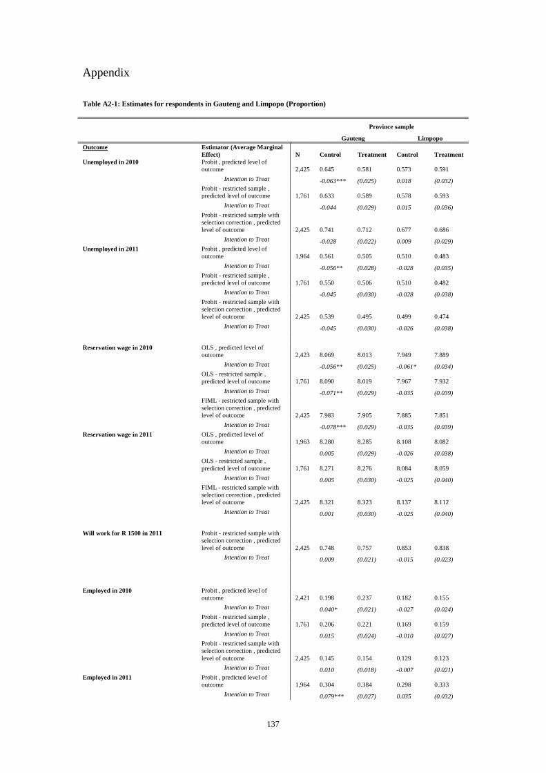
137

Appendix

Table A2-1: Estimates for respondents in Gauteng and Limpopo (Proportion)

Province sample

Gauteng Limpopo

Outcome Estimator (Average Marginal

Effect) N Control Treatment Control Treatment

Unemployed in 2010 Probit , predicted level of

outcome 2,425 0.645 0.581 0.573 0.591

Intention to Treat

-0.063*** (0.025) 0.018 (0.032)

Probit - restricted sample ,

predicted level of outcome 1,761 0.633 0.589 0.578 0.593

Intention to Treat

-0.044 (0.029) 0.015 (0.036)

Probit - restricted sample with

selection correction , predicted

level of outcome 2,425 0.741 0.712 0.677 0.686

Intention to Treat

-0.028 (0.022) 0.009 (0.029)

Unemployed in 2011 Probit , predicted level of

outcome 1,964 0.561 0.505 0.510 0.483

Intention to Treat

-0.056** (0.028) -0.028 (0.035)

Probit - restricted sample ,

predicted level of outcome 1,761 0.550 0.506 0.510 0.482

Intention to Treat

-0.045 (0.030) -0.028 (0.038)

Probit - restricted sample with

selection correction , predicted

level of outcome 2,425 0.539 0.495 0.499 0.474

Intention to Treat

-0.045 (0.030) -0.026 (0.038)

Reservation wage in 2010 OLS , predicted level of

outcome 2,423 8.069 8.013 7.949 7.889

Intention to Treat

-0.056** (0.025) -0.061* (0.034)

OLS - restricted sample ,

predicted level of outcome 1,761 8.090 8.019 7.967 7.932

Intention to Treat

-0.071** (0.029) -0.035 (0.039)

FIML - restricted sample with

selection correction , predicted

level of outcome 2,425 7.983 7.905 7.885 7.851

Intention to Treat

-0.078*** (0.029) -0.035 (0.039)

Reservation wage in 2011 OLS , predicted level of

outcome 1,963 8.280 8.285 8.108 8.082

Intention to Treat

0.005 (0.029) -0.026 (0.038)

OLS - restricted sample ,

predicted level of outcome 1,761 8.271 8.276 8.084 8.059

Intention to Treat

0.005 (0.030) -0.025 (0.040)

FIML - restricted sample with

selection correction , predicted

level of outcome 2,425 8.321 8.323 8.137 8.112

Intention to Treat

0.001 (0.030) -0.025 (0.040)

Will work for R 1500 in 2011 Probit - restricted sample with

selection correction , predicted

level of outcome 2,425 0.748 0.757 0.853 0.838

Intention to Treat

0.009 (0.021) -0.015 (0.023)

Employed in 2010 Probit , predicted level of

outcome 2,421 0.198 0.237 0.182 0.155

Intention to Treat

0.040* (0.021) -0.027 (0.024)

Probit - restricted sample ,

predicted level of outcome 1,761 0.206 0.221 0.169 0.159

Intention to Treat

0.015 (0.024) -0.010 (0.027)

Probit - restricted sample with

selection correction , predicted

level of outcome 2,425 0.145 0.154 0.129 0.123

Intention to Treat

0.010 (0.018) -0.007 (0.021)

Employed in 2011 Probit , predicted level of

outcome 1,964 0.304 0.384 0.298 0.333

Intention to Treat

0.079*** (0.027) 0.035 (0.032)

138

Probit - restricted sample ,

predicted level of outcome 1,761 0.309 0.386 0.296 0.326

Intention to Treat

0.077*** (0.028) 0.030 (0.035)

Probit - restricted sample with

selection correction , predicted

level of outcome 2,425 0.390 0.470 0.357 0.389

Intention to Treat

0.081*** (0.030) 0.033 (0.037)

Any job in 2011 Probit - restricted sample with

selection correction , predicted

level of outcome 2,425 0.364 0.442 0.346 0.366

Intention to Treat

0.078*** (0.030) 0.021 (0.036)

Self-reported employed in 2011 Probit - restricted sample with

selection correction , predicted

level of outcome 2,425 0.363 0.458 0.375 0.375

Intention to Treat

0.096** (0.042) 0.001 (0.036)

Employed in 2011 but unhappy in this

employment

Probit - restricted sample with

selection correction , predicted

level of outcome 2,425 0.291 0.351 0.219 0.251

Intention to Treat

0.060* (0.032) 0.032 (0.034)

Employed in 2011 and not unhappy in

this employment

Probit - restricted sample with

selection correction , predicted

level of outcome 2,425 0.151 0.173 0.168 0.180

Intention to Treat

0.022 (0.018) 0.011 (0.024)

Difference between earnings and

reservation wage in 2011

FIML - restricted sample with

selection correction , predicted

level of outcome 2,425 -3,700.581 -3,456.936 -3,351.042 -3,027.679

Intention to Treat

243.645 (173.327) 323.362 (217.326)

Unhappy, in general, in 2011 Probit - restricted sample with

selection correction , predicted

level of outcome 2,425 0.490 0.496 0.383 0.418

Intention to Treat

0.006 (0.028) 0.035 (0.035)

Full-time job in 2011 Probit - restricted sample with

selection correction , predicted

level of outcome 2,425 0.356 0.446 0.351 0.362

Intention to Treat

0.090*** (0.029) 0.011 (0.036)

Full-time job in 2011 but unhappy in

this job

Probit - restricted sample with

selection correction , predicted

level of outcome 2,425 0.271 0.330 0.213 0.222

Intention to Treat

0.059** (0.030) 0.010 (0.033)

Full-time job in 2011 and not unhappy

in this job

Probit - restricted sample with

selection correction , predicted

level of outcome 2,425 0.141 0.167 0.170 0.173

Intention to Treat

0.026 (0.018) 0.002 (0.024)

Full-time job in 2011 earning less than

reservation wage in 2011

Probit - restricted sample with

selection correction , predicted

level of outcome 2,425 0.383 0.449 0.345 0.374

Intention to Treat

0.066** (0.029) 0.029 (0.036)

Full-time job in 2011 earning less than

reservation wage in 2011 and unhappy

in this employment

Probit - restricted sample with

selection correction , predicted

level of outcome 2,425 0.291 0.340 0.222 0.228

Intention to Treat

0.050* (0.029) 0.006 (0.032)

Full-time job in 2011 earning less than

reservation wage in 2011 and not

unhappy in this job

Probit - restricted sample with

selection correction , predicted

level of outcome 2,425 0.172 0.196 0.182 0.198

Intention to Treat

0.023 (0.025) 0.015 (0.030)

Full-time job in 2011 earning less than

reservation wage in 2010

Probit - restricted sample with

selection correction , predicted

level of outcome 2,425 0.229 0.276 0.229 0.259

Intention to Treat

0.047* (0.028) 0.029 (0.034)

Full-time job in 2011 earning less than

reservation wage in 2010 and unhappy

in this employment

Probit - restricted sample with

selection correction , predicted

level of outcome 2,425 0.239 0.289 0.187 0.186

Intention to Treat

0.050* (0.030) -0.001 (0.033)

Full-time job in 2011 earning less than

reservation wage in 2010 and not

unhappy in this job

Probit - restricted sample with

selection correction , predicted

level of outcome 2,425 0.094 0.100 0.115 0.134

Intention to Treat

0.006 (0.017) 0.019 (0.023)

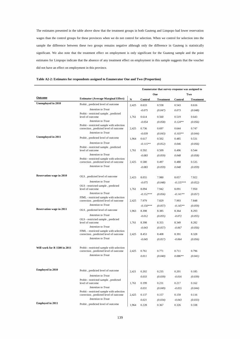
139

The estimates presented in the table above show that the treatment groups in both Gauteng and Limpopo had lower reservation

wages than the control groups for these provinces when we do not control for selection. When we control for selection into the

sample the difference between these two groups remains negative although only the difference in Gauteng is statistically

significant. We also note that the treatment effect on employment is only significant for the Guateng sample and the point

estimates for Limpopo indicate that the absence of any treatment effect on employment in this sample suggests that the voucher

did not have an effect on employment in this province.

Table A2-2: Estimates for respondents assigned to Enumerator One and Two (Proportion)

Enumerator that survey-response was assigned to

One Two

Outcome Estimator (Average Marginal Effect) N Control Treatment Control Treatment

Unemployed in 2010 Probit , predicted level of outcome 2,425 0.633 0.558 0.543 0.616

Intention to Treat

-0.075 (0.047) 0.073 (0.048)

Probit - restricted sample , predicted

level of outcome 1,761 0.614 0.560 0.519 0.643

Intention to Treat

-0.054 (0.058) 0.124** (0.056)

Probit - restricted sample with selection

correction , predicted level of outcome 2,425 0.736 0.697 0.644 0.747

Intention to Treat

-0.039 (0.043) 0.103** (0.044)

Unemployed in 2011 Probit , predicted level of outcome 1,964 0.617 0.502 0.485 0.531

Intention to Treat

-0.115** (0.052) 0.046 (0.056)

Probit - restricted sample , predicted

level of outcome 1,761 0.592 0.509 0.496 0.544

Intention to Treat

-0.083 (0.059) 0.048 (0.058)

Probit - restricted sample with selection

correction , predicted level of outcome 2,425 0.580 0.497 0.488 0.535

Intention to Treat

-0.083 (0.059) 0.048 (0.059)

Reservation wage in 2010 OLS , predicted level of outcome 2,423 8.055 7.980 8.057 7.922

Intention to Treat

-0.075 (0.048) -0.135*** (0.052)

OLS - restricted sample , predicted

level of outcome 1,761 8.094 7.942 8.091 7.950

Intention to Treat

-0.152*** (0.056) -0.141** (0.057)

FIML - restricted sample with selection

correction , predicted level of outcome 2,425 7.979 7.829 7.993 7.848

Intention to Treat

-0.150*** (0.057) -0.145** (0.059)

Reservation wage in 2011 OLS , predicted level of outcome 1,963 8.398 8.385 8.364 8.293

Intention to Treat

-0.012 (0.055) -0.072 (0.055)

OLS - restricted sample , predicted

level of outcome 1,761 8.398 8.355 8.349 8.282

Intention to Treat

-0.043 (0.057) -0.067 (0.056)

FIML - restricted sample with selection

correction , predicted level of outcome 2,425 8.453 8.408 8.391 8.328

Intention to Treat

-0.045 (0.057) -0.064 (0.056)

Will work for R 1500 in 2011 Probit - restricted sample with selection

correction , predicted level of outcome 2,425 0.761 0.771 0.711 0.796

Intention to Treat

0.011 (0.040) 0.086** (0.041)

Employed in 2010 Probit , predicted level of outcome 2,421 0.202 0.235 0.201 0.185

Intention to Treat

0.033 (0.039) -0.016 (0.039)

Probit - restricted sample , predicted

level of outcome 1,761 0.199 0.231 0.217 0.162

Intention to Treat

0.031 (0.049) -0.055 (0.044)

Probit - restricted sample with selection

correction , predicted level of outcome 2,425 0.137 0.157 0.159 0.116

Intention to Treat

0.021 (0.034) -0.043 (0.033)

Employed in 2011 Probit , predicted level of outcome 1,964 0.228 0.367 0.326 0.338

140

Intention to Treat

0.139*** (0.047) 0.012 (0.052)

Probit - restricted sample , predicted

level of outcome 1,761 0.245 0.368 0.321 0.336

Intention to Treat

0.122** (0.054) 0.015 (0.054)

Probit - restricted sample with selection

correction , predicted level of outcome 2,425 0.334 0.458 0.395 0.413

Intention to Treat

0.124** (0.060) 0.018 (0.057)

Any job in 2011 Probit - restricted sample with selection

correction , predicted level of outcome 2,425 0.345 0.425 0.364 0.402

Intention to Treat

0.080 (0.058) 0.037 (0.057)

Self-reported employed in 2011 Probit - restricted sample with selection

correction , predicted level of outcome 2,425 0.353 0.485 0.362 0.403

Intention to Treat

0.132 (0.081) 0.041 (0.056)

Employed in 2011 but unhappy

in this employment

Probit - restricted sample with selection

correction , predicted level of outcome 2,425 0.267 0.356 0.275 0.282

Intention to Treat

0.089 (0.070) 0.007 (0.053)

Employed in 2011 and not

unhappy in this employment

Probit - restricted sample with selection

correction , predicted level of outcome 2,425 0.130 0.166 0.162 0.177

Intention to Treat

0.035 (0.034) 0.014 (0.036)

Difference between earnings

and reservation wage in 2011

FIML - restricted sample with selection

correction , predicted level of outcome 2,425 -4,564.508 -3,917.017 -3,842.198 -3,574.744

Intention to Treat

647.491* (354.923) 267.454 (390.326)

Unhappy, in general, in 2011 Probit - restricted sample with selection

correction , predicted level of outcome 2,425 0.649 0.643 0.436 0.445

Intention to Treat

-0.006 (0.052) 0.009 (0.056)

The estimates presented in this table show that there is considerable heterogeneity in the treatment effect estimates across the

surveys that were assigned to one of the six enumerator groups in 2011.

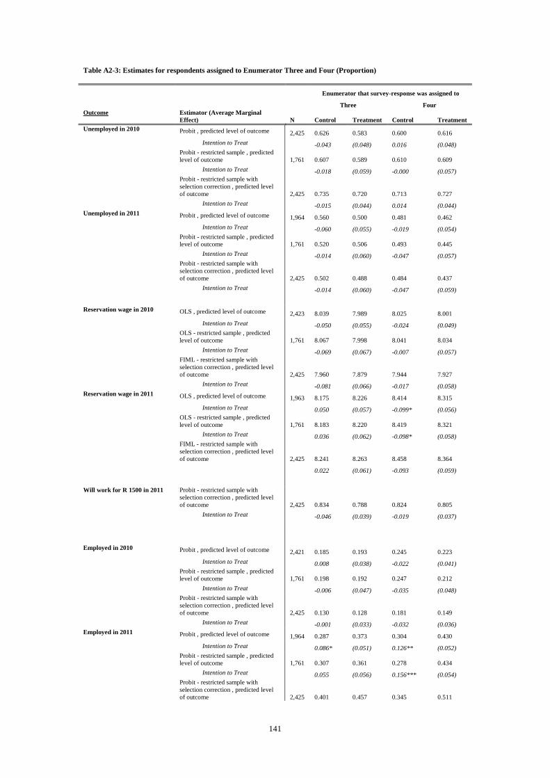
141

Table A2-3: Estimates for respondents assigned to Enumerator Three and Four (Proportion)

Enumerator that survey-response was assigned to

Three Four

Outcome Estimator (Average Marginal

Effect) N Control Treatment Control Treatment

Unemployed in 2010 Probit , predicted level of outcome 2,425 0.626 0.583 0.600 0.616

Intention to Treat

-0.043 (0.048) 0.016 (0.048)

Probit - restricted sample , predicted

level of outcome 1,761 0.607 0.589 0.610 0.609

Intention to Treat

-0.018 (0.059) -0.000 (0.057)

Probit - restricted sample with

selection correction , predicted level

of outcome 2,425 0.735 0.720 0.713 0.727

Intention to Treat

-0.015 (0.044) 0.014 (0.044)

Unemployed in 2011 Probit , predicted level of outcome 1,964 0.560 0.500 0.481 0.462

Intention to Treat

-0.060 (0.055) -0.019 (0.054)

Probit - restricted sample , predicted

level of outcome 1,761 0.520 0.506 0.493 0.445

Intention to Treat

-0.014 (0.060) -0.047 (0.057)

Probit - restricted sample with

selection correction , predicted level

of outcome 2,425 0.502 0.488 0.484 0.437

Intention to Treat

-0.014 (0.060) -0.047 (0.059)

Reservation wage in 2010 OLS , predicted level of outcome 2,423 8.039 7.989 8.025 8.001

Intention to Treat

-0.050 (0.055) -0.024 (0.049)

OLS - restricted sample , predicted

level of outcome 1,761 8.067 7.998 8.041 8.034

Intention to Treat

-0.069 (0.067) -0.007 (0.057)

FIML - restricted sample with

selection correction , predicted level

of outcome 2,425 7.960 7.879 7.944 7.927

Intention to Treat

-0.081 (0.066) -0.017 (0.058)

Reservation wage in 2011 OLS , predicted level of outcome 1,963 8.175 8.226 8.414 8.315

Intention to Treat

0.050 (0.057) -0.099* (0.056)

OLS - restricted sample , predicted

level of outcome 1,761 8.183 8.220 8.419 8.321

Intention to Treat

0.036 (0.062) -0.098* (0.058)

FIML - restricted sample with

selection correction , predicted level

of outcome 2,425 8.241 8.263 8.458 8.364

0.022 (0.061) -0.093 (0.059)

Will work for R 1500 in 2011 Probit - restricted sample with

selection correction , predicted level

of outcome 2,425 0.834 0.788 0.824 0.805

Intention to Treat

-0.046 (0.039) -0.019 (0.037)

Employed in 2010 Probit , predicted level of outcome 2,421 0.185 0.193 0.245 0.223

Intention to Treat

0.008 (0.038) -0.022 (0.041)

Probit - restricted sample , predicted

level of outcome 1,761 0.198 0.192 0.247 0.212

Intention to Treat

-0.006 (0.047) -0.035 (0.048)

Probit - restricted sample with

selection correction , predicted level

of outcome 2,425 0.130 0.128 0.181 0.149

Intention to Treat

-0.001 (0.033) -0.032 (0.036)

Employed in 2011 Probit , predicted level of outcome 1,964 0.287 0.373 0.304 0.430

Intention to Treat

0.086* (0.051) 0.126** (0.052)

Probit - restricted sample , predicted

level of outcome 1,761 0.307 0.361 0.278 0.434

Intention to Treat

0.055 (0.056) 0.156*** (0.054)

Probit - restricted sample with

selection correction , predicted level

of outcome 2,425 0.401 0.457 0.345 0.511

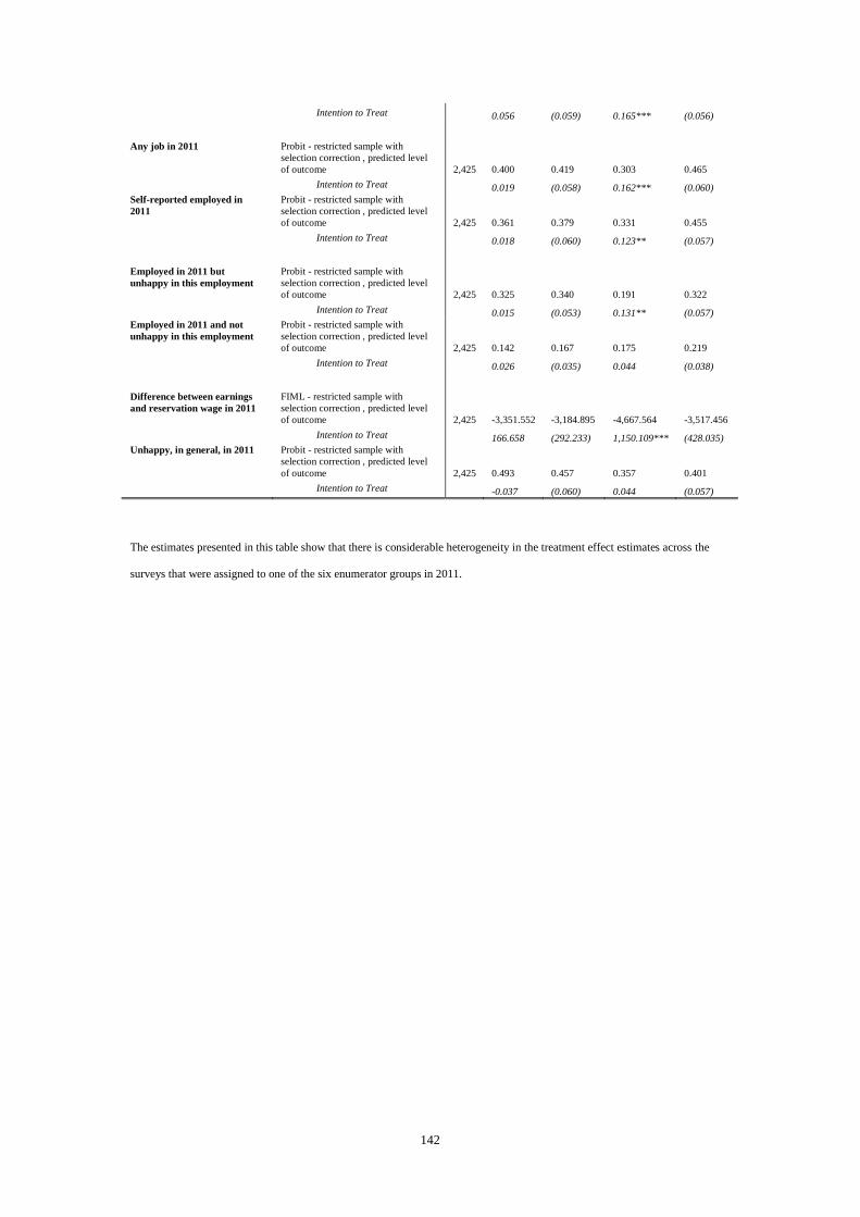
142

Intention to Treat

0.056 (0.059) 0.165*** (0.056)

Any job in 2011 Probit - restricted sample with

selection correction , predicted level

of outcome 2,425 0.400 0.419 0.303 0.465

Intention to Treat

0.019 (0.058) 0.162*** (0.060)

Self-reported employed in

2011

Probit - restricted sample with

selection correction , predicted level

of outcome 2,425 0.361 0.379 0.331 0.455

Intention to Treat

0.018 (0.060) 0.123** (0.057)

Employed in 2011 but

unhappy in this employment

Probit - restricted sample with

selection correction , predicted level

of outcome 2,425 0.325 0.340 0.191 0.322

Intention to Treat

0.015 (0.053) 0.131** (0.057)

Employed in 2011 and not

unhappy in this employment

Probit - restricted sample with

selection correction , predicted level

of outcome 2,425 0.142 0.167 0.175 0.219

Intention to Treat

0.026 (0.035) 0.044 (0.038)

Difference between earnings

and reservation wage in 2011

FIML - restricted sample with

selection correction , predicted level

of outcome 2,425 -3,351.552 -3,184.895 -4,667.564 -3,517.456

Intention to Treat

166.658 (292.233) 1,150.109*** (428.035)

Unhappy, in general, in 2011 Probit - restricted sample with

selection correction , predicted level

of outcome 2,425 0.493 0.457 0.357 0.401

Intention to Treat

-0.037 (0.060) 0.044 (0.057)

The estimates presented in this table show that there is considerable heterogeneity in the treatment effect estimates across the

surveys that were assigned to one of the six enumerator groups in 2011.

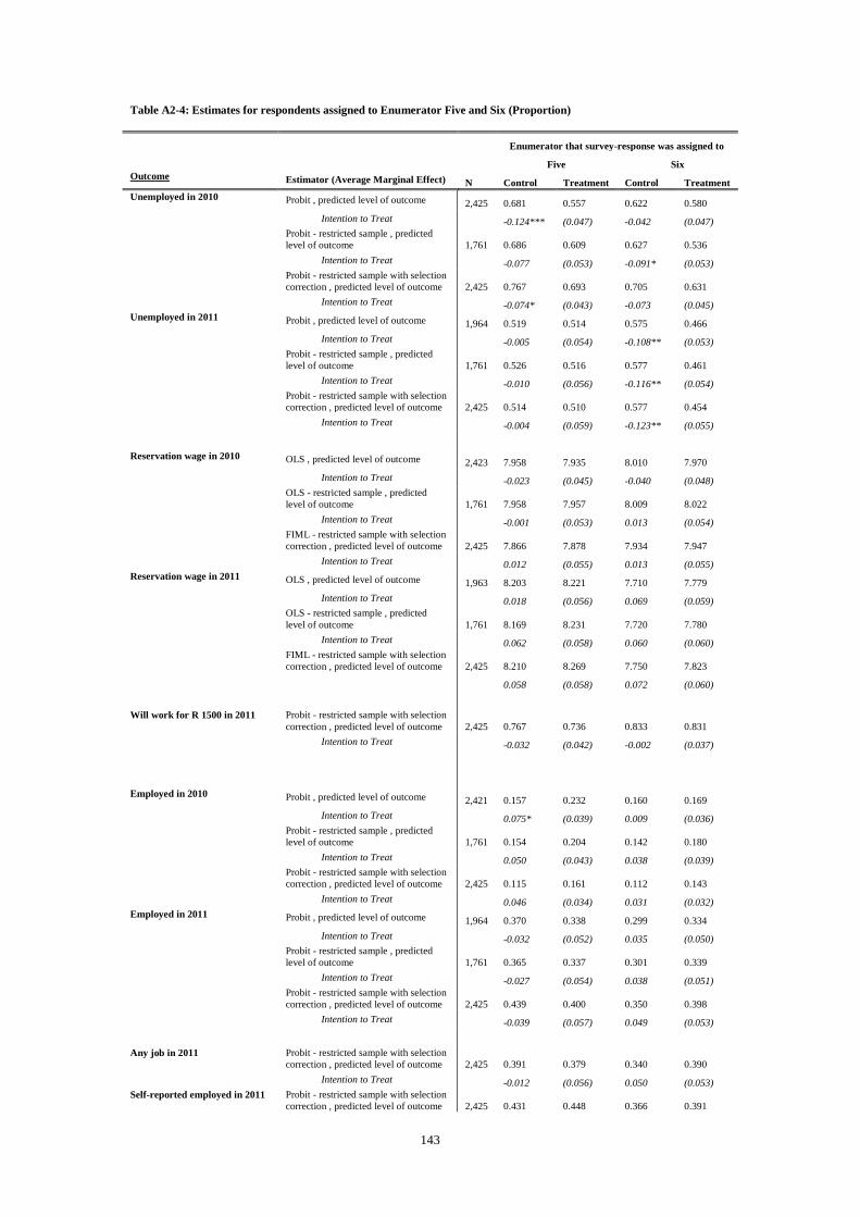
143

Table A2-4: Estimates for respondents assigned to Enumerator Five and Six (Proportion)

Enumerator that survey-response was assigned to

Five Six

Outcome Estimator (Average Marginal Effect) N Control Treatment Control Treatment

Unemployed in 2010 Probit , predicted level of outcome 2,425 0.681 0.557 0.622 0.580

Intention to Treat

-0.124*** (0.047) -0.042 (0.047)

Probit - restricted sample , predicted

level of outcome 1,761 0.686 0.609 0.627 0.536

Intention to Treat

-0.077 (0.053) -0.091* (0.053)

Probit - restricted sample with selection

correction , predicted level of outcome 2,425 0.767 0.693 0.705 0.631

Intention to Treat

-0.074* (0.043) -0.073 (0.045)

Unemployed in 2011 Probit , predicted level of outcome 1,964 0.519 0.514 0.575 0.466

Intention to Treat

-0.005 (0.054) -0.108** (0.053)

Probit - restricted sample , predicted

level of outcome 1,761 0.526 0.516 0.577 0.461

Intention to Treat

-0.010 (0.056) -0.116** (0.054)

Probit - restricted sample with selection

correction , predicted level of outcome 2,425 0.514 0.510 0.577 0.454

Intention to Treat

-0.004 (0.059) -0.123** (0.055)

Reservation wage in 2010 OLS , predicted level of outcome 2,423 7.958 7.935 8.010 7.970

Intention to Treat

-0.023 (0.045) -0.040 (0.048)

OLS - restricted sample , predicted

level of outcome 1,761 7.958 7.957 8.009 8.022

Intention to Treat

-0.001 (0.053) 0.013 (0.054)

FIML - restricted sample with selection

correction , predicted level of outcome 2,425 7.866 7.878 7.934 7.947

Intention to Treat

0.012 (0.055) 0.013 (0.055)

Reservation wage in 2011 OLS , predicted level of outcome 1,963 8.203 8.221 7.710 7.779

Intention to Treat

0.018 (0.056) 0.069 (0.059)

OLS - restricted sample , predicted

level of outcome 1,761 8.169 8.231 7.720 7.780

Intention to Treat

0.062 (0.058) 0.060 (0.060)

FIML - restricted sample with selection

correction , predicted level of outcome 2,425 8.210 8.269 7.750 7.823

0.058 (0.058) 0.072 (0.060)

Will work for R 1500 in 2011 Probit - restricted sample with selection

correction , predicted level of outcome 2,425 0.767 0.736 0.833 0.831

Intention to Treat

-0.032 (0.042) -0.002 (0.037)

Employed in 2010 Probit , predicted level of outcome 2,421 0.157 0.232 0.160 0.169

Intention to Treat

0.075* (0.039) 0.009 (0.036)

Probit - restricted sample , predicted

level of outcome 1,761 0.154 0.204 0.142 0.180

Intention to Treat

0.050 (0.043) 0.038 (0.039)

Probit - restricted sample with selection

correction , predicted level of outcome 2,425 0.115 0.161 0.112 0.143

Intention to Treat

0.046 (0.034) 0.031 (0.032)

Employed in 2011 Probit , predicted level of outcome 1,964 0.370 0.338 0.299 0.334

Intention to Treat

-0.032 (0.052) 0.035 (0.050)

Probit - restricted sample , predicted

level of outcome 1,761 0.365 0.337 0.301 0.339

Intention to Treat

-0.027 (0.054) 0.038 (0.051)

Probit - restricted sample with selection

correction , predicted level of outcome 2,425 0.439 0.400 0.350 0.398

Intention to Treat

-0.039 (0.057) 0.049 (0.053)

Any job in 2011 Probit - restricted sample with selection

correction , predicted level of outcome 2,425 0.391 0.379 0.340 0.390

Intention to Treat

-0.012 (0.056) 0.050 (0.053)

Self-reported employed in 2011 Probit - restricted sample with selection

correction , predicted level of outcome 2,425 0.431 0.448 0.366 0.391

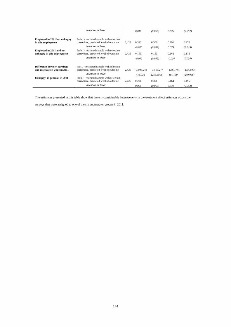
144

Intention to Treat

0.016 (0.066) 0.026 (0.052)

Employed in 2011 but unhappy

in this employment

Probit - restricted sample with selection

correction , predicted level of outcome 2,425 0.333 0.306 0.191 0.270

Intention to Treat

-0.026 (0.049) 0.079 (0.049)

Employed in 2011 and not

unhappy in this employment

Probit - restricted sample with selection

correction , predicted level of outcome 2,425 0.155 0.153 0.182 0.172

Intention to Treat

-0.002 (0.035) -0.010 (0.038)

Difference between earnings

and reservation wage in 2011

FIML - restricted sample with selection

correction , predicted level of outcome 2,425 -3,098.243 -3,516.277 -1,861.744 -2,042.904

Intention to Treat

-418.034 (255.680) -181.159 (240.068)

Unhappy, in general, in 2011 Probit - restricted sample with selection

correction , predicted level of outcome 2,425 0.291 0.351 0.464 0.496

Intention to Treat

0.060 (0.060) 0.031 (0.053)

The estimates presented in this table show that there is considerable heterogeneity in the treatment effect estimates across the

surveys that were assigned to one of the six enumerator groups in 2011.

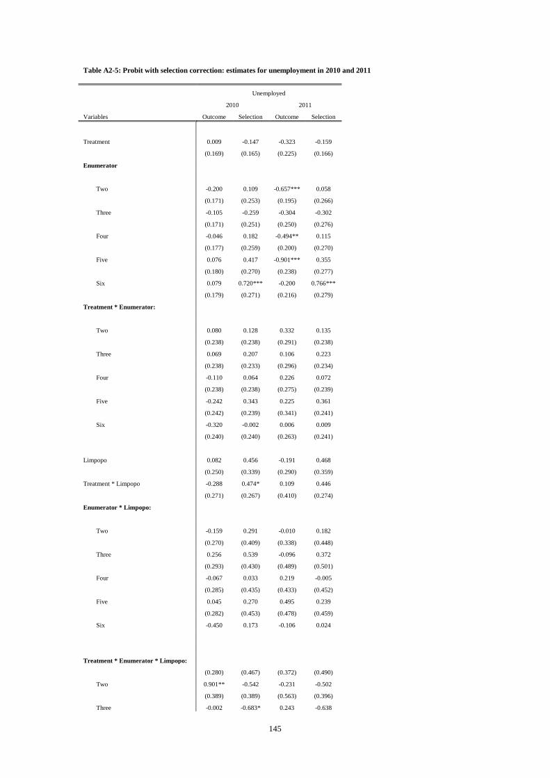
145

Table A2-5: Probit with selection correction: estimates for unemployment in 2010 and 2011

Unemployed

2010 2011

Variables Outcome Selection Outcome Selection

Treatment 0.009 -0.147 -0.323 -0.159

(0.169) (0.165) (0.225) (0.166)

Enumerator

Two -0.200 0.109 -0.657*** 0.058

(0.171) (0.253) (0.195) (0.266)

Three -0.105 -0.259 -0.304 -0.302

(0.171) (0.251) (0.250) (0.276)

Four -0.046 0.182 -0.494** 0.115

(0.177) (0.259) (0.200) (0.270)

Five 0.076 0.417 -0.901*** 0.355

(0.180) (0.270) (0.238) (0.277)

Six 0.079 0.720*** -0.200 0.766***

(0.179) (0.271) (0.216) (0.279)

Treatment * Enumerator:

Two 0.080 0.128 0.332 0.135

(0.238) (0.238) (0.291) (0.238)

Three 0.069 0.207 0.106 0.223

(0.238) (0.233) (0.296) (0.234)

Four -0.110 0.064 0.226 0.072

(0.238) (0.238) (0.275) (0.239)

Five -0.242 0.343 0.225 0.361

(0.242) (0.239) (0.341) (0.241)

Six -0.320 -0.002 0.006 0.009

(0.240) (0.240) (0.263) (0.241)

Limpopo 0.082 0.456 -0.191 0.468

(0.250) (0.339) (0.290) (0.359)

Treatment * Limpopo -0.288 0.474* 0.109 0.446

(0.271) (0.267) (0.410) (0.274)

Enumerator * Limpopo:

Two -0.159 0.291 -0.010 0.182

(0.270) (0.409) (0.338) (0.448)

Three 0.256 0.539 -0.096 0.372

(0.293) (0.430) (0.489) (0.501)

Four -0.067 0.033 0.219 -0.005

(0.285) (0.435) (0.433) (0.452)

Five 0.045 0.270 0.495 0.239

(0.282) (0.453) (0.478) (0.459)

Six -0.450 0.173 -0.106 0.024

Treatment * Enumerator * Limpopo:

(0.280) (0.467) (0.372) (0.490)

Two 0.901** -0.542 -0.231 -0.502

(0.389) (0.389) (0.563) (0.396)

Three -0.002 -0.683* 0.243 -0.638

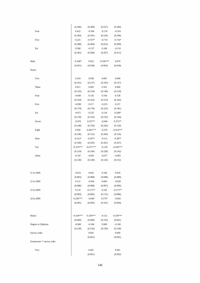
146

(0.390) (0.389) (0.527) (0.390)

Four 0.422 -0.594 -0.176 -0.554

(0.383) (0.391) (0.536) (0.396)

Five 0.225 -0.767* -0.714 -0.716*

(0.388) (0.404) (0.655) (0.409)

Six 0.568 -0.137 0.184 -0.110

(0.381) (0.399) (0.437) (0.411)

Male -0.108* 0.052 -0.250*** 0.079

(0.055) (0.058) (0.063) (0.058)

Strata:

Two 0.193 0.058 0.007 0.049

(0.161) (0.157) (0.183) (0.157)

Three 0.011 0.065 0.101 0.069

(0.120) (0.118) (0.149) (0.119)

Four -0.040 0.126 0.104 0.128

(0.164) (0.162) (0.215) (0.162)

Five -0.098 0.217 -0.225 0.227

(0.174) (0.178) (0.222) (0.181)

Six -0.071 0.235 0.134 0.248*

(0.139) (0.145) (0.232) (0.144)

Seven -0.070 0.357** -0.040 0.372**

(0.148) (0.156) (0.245) (0.156)

Eight 0.056 -0.401*** -0.276 -0.414***

(0.146) (0.155) (0.260) (0.156)

Nine -0.313* -0.397* -0.112 -0.387*

(0.189) (0.203) (0.281) (0.207)

Ten -0.374*** -0.471*** -0.150 -0.429***

(0.124) (0.140) (0.228) (0.142)

Other -0.197 -0.091 -0.077 -0.083

(0.130) (0.149) (0.143) (0.151)

21 in 2009 -0.023 0.042 0.106 0.029

(0.083) (0.088) (0.098) (0.089)

22 in 2009 0.121 -0.036 0.093 -0.028

(0.086) (0.088) (0.097) (0.090)

23 in 2009 0.110 -0.175** 0.102 -0.175**

(0.083) (0.085) (0.115) (0.086)

24 in 2009 0.236*** -0.049 0.179* -0.043

(0.091) (0.093) (0.101) (0.094)

Matric -0.330*** 0.318*** -0.121 0.328***

(0.060) (0.060) (0.152) (0.061)

Degree or Diploma -0.068 -0.184 0.068 -0.160

(0.130) (0.136) (0.159) (0.138)

Survey order

0.001

0.000

(0.001)

(0.001)

Enumerator * survey order

Two

0.001

0.001

(0.001)

(0.002)

147

Three

0.000

0.001

(0.001)

(0.002)

Four

-0.001

-0.000

(0.001)

(0.002)

Five

-0.003*

-0.002

(0.002)

(0.002)

Six

-0.003**

-0.004**

(0.002)

(0.002)

Limpopo * survey order

-0.004*

-0.004

(0.002)

(0.003)

Enumerator * Limpopo * survey order

Two

-0.000

0.001

(0.003)

(0.004)

Three

0.004

0.006

(0.003)

(0.005)

Four

0.007*

0.007*

(0.003)

(0.004)

Five

0.003

0.004

(0.004)

(0.004)

Six

0.004

0.005

(0.004)

(0.004)

dpn

0.079**

0.069

(0.033)

(0.044)

lg

0.014

-0.001

(0.064)

(0.073)

Limpopo * dpn

-0.119**

-0.109*

(0.059)

(0.064)

Limpopo * lg

0.260**

0.274**

(0.112)

(0.121)

-8.644

-0.388

(143.855)

(0.983)

Constant 0.812*** 0.039 0.528 0.066

(0.181) (0.226) (0.564) (0.232)

Observations 2,425 2,425 2,425 2,425

Bootstrapped standard errors in parentheses. *** p<0.01, ** p<0.05, * p<0.1.

The estimates presented in this table show that there is a statistically significant relationship between the exclusion restrictions

and selection into the sample.

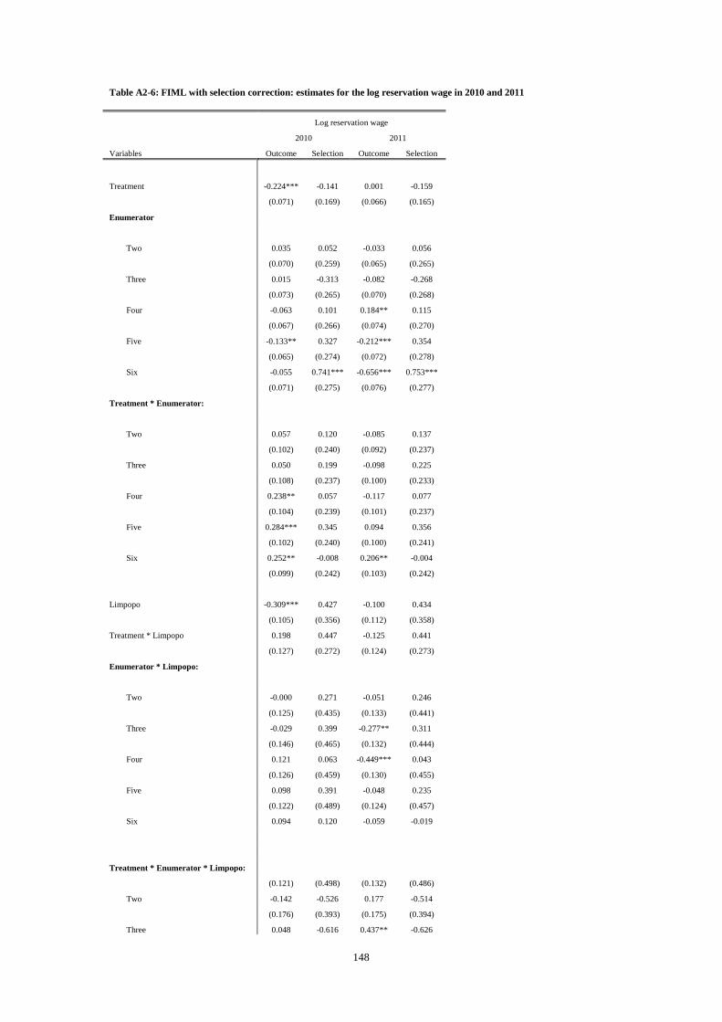
148

Table A2-6: FIML with selection correction: estimates for the log reservation wage in 2010 and 2011

Log reservation wage

2010 2011

Variables Outcome Selection Outcome Selection

Treatment -0.224*** -0.141 0.001 -0.159

(0.071) (0.169) (0.066) (0.165)

Enumerator

Two 0.035 0.052 -0.033 0.056

(0.070) (0.259) (0.065) (0.265)

Three 0.015 -0.313 -0.082 -0.268

(0.073) (0.265) (0.070) (0.268)

Four -0.063 0.101 0.184** 0.115

(0.067) (0.266) (0.074) (0.270)

Five -0.133** 0.327 -0.212*** 0.354

(0.065) (0.274) (0.072) (0.278)

Six -0.055 0.741*** -0.656*** 0.753***

(0.071) (0.275) (0.076) (0.277)

Treatment * Enumerator:

Two 0.057 0.120 -0.085 0.137

(0.102) (0.240) (0.092) (0.237)

Three 0.050 0.199 -0.098 0.225

(0.108) (0.237) (0.100) (0.233)

Four 0.238** 0.057 -0.117 0.077

(0.104) (0.239) (0.101) (0.237)

Five 0.284*** 0.345 0.094 0.356

(0.102) (0.240) (0.100) (0.241)

Six 0.252** -0.008 0.206** -0.004

(0.099) (0.242) (0.103) (0.242)

Limpopo -0.309*** 0.427 -0.100 0.434

(0.105) (0.356) (0.112) (0.358)

Treatment * Limpopo 0.198 0.447 -0.125 0.441

(0.127) (0.272) (0.124) (0.273)

Enumerator * Limpopo:

Two -0.000 0.271 -0.051 0.246

(0.125) (0.435) (0.133) (0.441)

Three -0.029 0.399 -0.277** 0.311

(0.146) (0.465) (0.132) (0.444)

Four 0.121 0.063 -0.449*** 0.043

(0.126) (0.459) (0.130) (0.455)

Five 0.098 0.391 -0.048 0.235

(0.122) (0.489) (0.124) (0.457)

Six 0.094 0.120 -0.059 -0.019

Treatment * Enumerator * Limpopo:

(0.121) (0.498) (0.132) (0.486)

Two -0.142 -0.526 0.177 -0.514

(0.176) (0.393) (0.175) (0.394)

Three 0.048 -0.616 0.437** -0.626

149

(0.192) (0.400) (0.178) (0.391)

Four -0.279 -0.540 0.182 -0.556

(0.178) (0.396) (0.171) (0.394)

Five -0.324* -0.712* 0.027 -0.694*

(0.174) (0.407) (0.170) (0.410)

Six -0.236 -0.098 -0.231 -0.086

(0.164) (0.408) (0.172) (0.408)

Male 0.104*** 0.072 0.133*** 0.082

(0.026) (0.059) (0.025) (0.058)

Strata:

Two -0.117 0.056 0.080 0.052

(0.075) (0.156) (0.067) (0.155)

Three -0.121** 0.071 0.001 0.074

(0.057) (0.119) (0.051) (0.119)

Four -0.086 0.118 -0.063 0.130

(0.078) (0.163) (0.064) (0.162)

Five 0.015 0.191 0.048 0.220

(0.077) (0.185) (0.081) (0.179)

Six -0.060 0.216 -0.130** 0.246*

(0.067) (0.152) (0.058) (0.144)

Seven 0.015 0.348** -0.080 0.372**

(0.072) (0.161) (0.065) (0.156)

Eight -0.016 -0.404** -0.105* -0.421***

(0.063) (0.158) (0.058) (0.155)

Nine 0.101 -0.399** 0.086 -0.393*

(0.080) (0.201) (0.089) (0.205)

Ten 0.222*** -0.388** 0.153** -0.423***

(0.066) (0.167) (0.060) (0.144)

Other 0.025 -0.069 -0.056 -0.092

(0.054) (0.156) (0.054) (0.150)

21 in 2009 0.024 0.018 0.061* 0.028

(0.037) (0.089) (0.036) (0.088)

22 in 2009 0.061 -0.032 0.090** -0.022

(0.038) (0.089) (0.039) (0.089)

23 in 2009 0.002 -0.180** 0.114*** -0.174**

(0.040) (0.086) (0.040) (0.086)

24 in 2009 0.029 -0.051 0.085** -0.044

(0.040) (0.094) (0.040) (0.094)

Matric 0.228*** 0.337*** 0.228*** 0.332***

(0.040) (0.063) (0.027) (0.061)

Degree or Diploma 0.176*** -0.155 0.295*** -0.153

(0.068) (0.138) (0.072) (0.138)

Survey order

0.000

0.000

(0.001)

(0.001)

Enumerator * survey order

Two

0.001

0.001

(0.002)

(0.002)

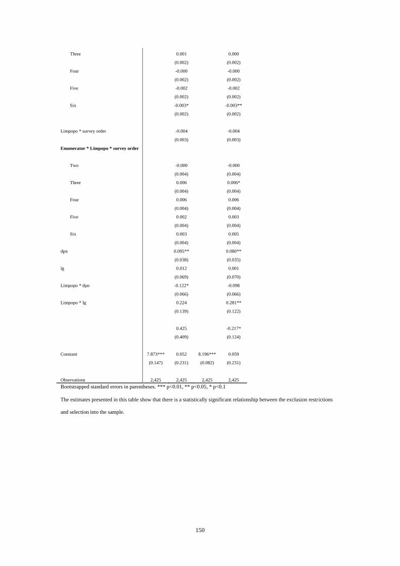
150

Three

0.001

0.000

(0.002)

(0.002)

Four

-0.000

-0.000

(0.002)

(0.002)

Five

-0.002

-0.002

(0.002)

(0.002)

Six

-0.003*

-0.003**

(0.002)

(0.002)

Limpopo * survey order

-0.004

-0.004

(0.003)

(0.003)

Enumerator * Limpopo * survey order

Two

-0.000

-0.000

(0.004)

(0.004)

Three

0.006

0.006*

(0.004)

(0.004)

Four

0.006

0.006

(0.004)

(0.004)

Five

0.002

0.003

(0.004)

(0.004)

Six

0.003

0.005

(0.004)

(0.004)

dpn

0.095**

0.080**

(0.038)

(0.035)

lg

0.012

0.001

(0.069)

(0.070)

Limpopo * dpn

-0.122*

-0.098

(0.066)

(0.066)

Limpopo * lg

0.224

0.281**

(0.139)

(0.122)

0.425

-0.217*

(0.409)

(0.124)

Constant 7.873*** 0.052 8.196*** 0.059

(0.147) (0.231) (0.082) (0.231)

Observations 2,425 2,425 2,425 2,425

Bootstrapped standard errors in parentheses. *** p<0.01, ** p<0.05, * p<0.1

The estimates presented in this table show that there is a statistically significant relationship between the exclusion restrictions

and selection into the sample.

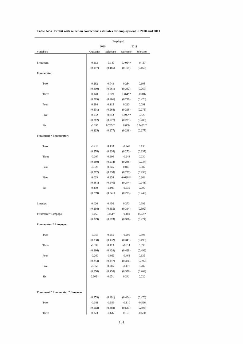
151

Table A2-7: Probit with selection correction: estimates for employment in 2010 and 2011

Employed

2010 2011

Variables Outcome Selection Outcome Selection

Treatment 0.113 -0.149 0.405** -0.167

(0.197) (0.166) (0.199) (0.166)

Enumerator

Two 0.262 0.043 0.284 0.103

(0.200) (0.261) (0.232) (0.269)

Three 0.140 -0.371 0.464** -0.316

(0.205) (0.266) (0.210) (0.278)

Four 0.284 0.115 0.213 0.091

(0.201) (0.268) (0.218) (0.273)

Five 0.032 0.313 0.495** 0.320

(0.212) (0.277) (0.231) (0.283)

Six -0.355 0.705** 0.006 0.742***

(0.235) (0.277) (0.248) (0.277)

Treatment * Enumerator:

Two -0.210 0.133 -0.249 0.139

(0.278) (0.238) (0.273) (0.237)

Three -0.207 0.200 -0.244 0.230

(0.280) (0.234) (0.288) (0.234)

Four -0.326 0.045 0.027 0.082

(0.272) (0.238) (0.277) (0.238)

Five 0.033 0.358 -0.638** 0.364

(0.281) (0.240) (0.274) (0.241)

Six 0.430 -0.009 -0.035 0.009

(0.299) (0.241) (0.275) (0.242)

Limpopo 0.026 0.456 0.273 0.392

(0.298) (0.355) (0.314) (0.392)

Treatment * Limpopo -0.053 0.461* -0.181 0.459*

(0.329) (0.273) (0.376) (0.274)

Enumerator * Limpopo:

Two -0.355 0.255 -0.209 0.304

(0.338) (0.432) (0.341) (0.493)

Three -0.399 0.413 -0.614 0.390

(0.366) (0.439) (0.428) (0.496)

Four -0.260 -0.055 -0.463 0.135

(0.343) (0.447) (0.376) (0.592)

Five -0.350 0.285 -0.477 0.287

(0.358) (0.458) (0.370) (0.462)

Six 0.602* 0.051 0.241 0.020

Treatment * Enumerator * Limpopo:

(0.353) (0.491) (0.404) (0.476)

Two -0.381 -0.551 -0.110 -0.526

(0.502) (0.393) (0.533) (0.395)

Three 0.323 -0.637 0.151 -0.630

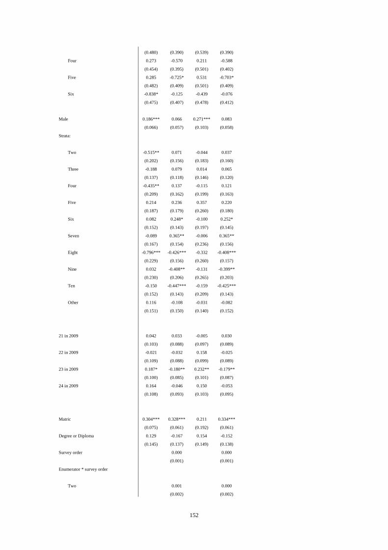
152

(0.480) (0.390) (0.539) (0.390)

Four 0.273 -0.570 0.211 -0.588

(0.454) (0.395) (0.501) (0.402)

Five 0.285 -0.725* 0.531 -0.703*

(0.482) (0.409) (0.501) (0.409)

Six -0.838* -0.125 -0.439 -0.076

(0.475) (0.407) (0.478) (0.412)

Male 0.186*** 0.066 0.271*** 0.083

(0.066) (0.057) (0.103) (0.058)

Strata:

Two -0.515** 0.071 -0.044 0.037

(0.202) (0.156) (0.183) (0.160)

Three -0.188 0.079 0.014 0.065

(0.137) (0.118) (0.146) (0.120)

Four -0.435** 0.137 -0.115 0.121

(0.209) (0.162) (0.199) (0.163)

Five 0.214 0.236 0.357 0.220

(0.187) (0.179) (0.260) (0.180)

Six 0.082 0.248* -0.100 0.252*

(0.152) (0.143) (0.197) (0.145)

Seven -0.089 0.365** -0.006 0.365**

(0.167) (0.154) (0.236) (0.156)

Eight -0.796*** -0.426*** -0.332 -0.408***

(0.229) (0.156) (0.260) (0.157)

Nine 0.032 -0.408** -0.131 -0.399**

(0.230) (0.206) (0.265) (0.203)

Ten -0.150 -0.447*** -0.159 -0.425***

(0.152) (0.143) (0.209) (0.143)

Other 0.116 -0.108 -0.031 -0.082

(0.151) (0.150) (0.140) (0.152)

21 in 2009 0.042 0.033 -0.005 0.030

(0.103) (0.088) (0.097) (0.089)

22 in 2009 -0.021 -0.032 0.158 -0.025

(0.109) (0.088) (0.099) (0.089)

23 in 2009 0.187* -0.180** 0.232** -0.179**

(0.100) (0.085) (0.101) (0.087)

24 in 2009 0.164 -0.046 0.150 -0.053

(0.108) (0.093) (0.103) (0.095)

Matric 0.304*** 0.328*** 0.211 0.334***

(0.075) (0.061) (0.192) (0.061)

Degree or Diploma 0.129 -0.167 0.154 -0.152

(0.145) (0.137) (0.149) (0.138)

Survey order

0.000

0.000

(0.001)

(0.001)

Enumerator * survey order

Two

0.001

0.000

(0.002)

(0.002)

153

Three

0.001

0.001

(0.002)

(0.002)

Four

-0.000

-0.000

(0.002)

(0.002)

Five

-0.002

-0.002

(0.002)

(0.002)

Six

-0.003*

-0.003**

(0.002)

(0.002)

Limpopo * survey order

-0.004

-0.003

(0.003)

(0.003)

Enumerator * Limpopo * survey order

Two

-0.000

-0.001

(0.004)

(0.005)

Three

0.006

0.006

(0.004)

(0.005)

Four

0.008**

0.005

(0.004)

(0.006)

Five

0.003

0.003

(0.004)

(0.004)

Six

0.004

0.004

(0.004)

(0.004)

dpn

0.083**

0.075**

(0.034)

(0.035)

lg

0.003

0.017

(0.068)

(0.073)

Limpopo * dpn

-0.104

-0.106*

(0.064)

(0.064)

Limpopo * lg

0.256**

0.253*

(0.120)

(0.130)

1.717***

-0.476

(0.587)

(0.857)

Constant -1.403*** 0.100 -0.909 0.079

(0.218) (0.234) (0.720) (0.233)

Observations 2,425 2,425 2,425 2,425

Bootstrapped standard errors in parentheses. *** p<0.01, ** p<0.05, * p<0.1

The estimates presented in this table show that there is a statistically significant relationship between the exclusion restrictions

and selection into the sample.

154

A2-8: Brochure text

The African Micro-Economic Research Umbrella (AMERU) at the University of the

Witwatersrand is conducting a trial to assess the impact of a targeted wage subsidy on the

employment of young people in South Africa.

A randomly selected group of individuals aged from 20 to 24 years has been assigned an

identification card that verifies that the firms who employ them are entitled to receive a

subsidy that covers a portion of the wage these firms pay to them while they are employed at

the firms.

The total value of the subsidy is R5,000. Payments will be made in monthly instalments to the

firms until this amount is exhausted and provided the card holder remains employed by the

firm. The value of the monthly payments will be calculated as follows:

It will be up to half the person’s wage if the wage is less than R 1,667 per month

It will be equal to R 833 per month if the wage is greater than or equal to R1,667 per month

The subsidy is transferable in those cases where a candidate leaves or is laid off before the R

5000 is exhausted but will only cover the balance that remains after any previous payments

have been subtracted.

The project will run until February 2011. This is the final month in which payments will

made.

In order for businesses to qualify for this subsidy they must be formally registered (have a

company number) and they must be registered with the South African Revenue Service (have

a VAT registration or income tax number) or be registered with the Unemployment Insurance

Fund (UIF).

The candidates in the trial must be employed full-time, but can be employed on a contract

basis, and are covered by standard South African labour laws.

The business will not be taxed on the amount they receive as the subsidy

Every effort will be made to ensure that the administrative burden on firms is minimal.

It is important to note that that the candidates in this trial are not endorsed by the University

of the Witwatersrand.

Furthermore, firms who wish to employ a candidate should do so for commercial reasons

only. This simply means that firms should treat the candidate in the same way they would

anyone they would normally employ.

The University of the Witwatersrand cannot be held responsible for the actions of the

candidate.

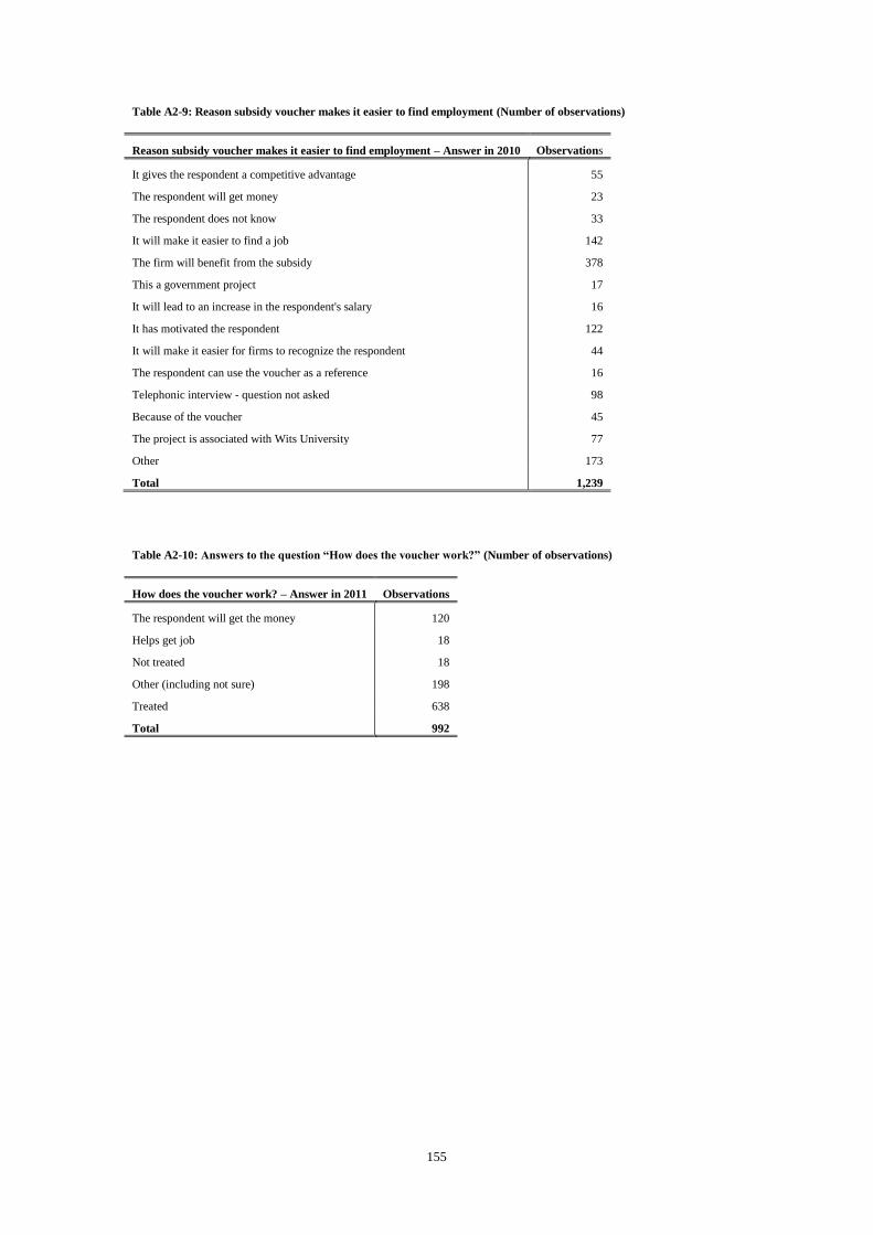
155

Table A2-9: Reason subsidy voucher makes it easier to find employment (Number of observations)

Reason subsidy voucher makes it easier to find employment – Answer in 2010 Observations

It gives the respondent a competitive advantage 55

The respondent will get money 23

The respondent does not know 33

It will make it easier to find a job 142

The firm will benefit from the subsidy 378

This a government project 17

It will lead to an increase in the respondent's salary 16

It has motivated the respondent 122

It will make it easier for firms to recognize the respondent 44

The respondent can use the voucher as a reference 16

Telephonic interview - question not asked 98

Because of the voucher 45

The project is associated with Wits University 77

Other 173

Total 1,239

Table A2-10: Answers to the question “How does the voucher work?” (Number of observations)

How does the voucher work? – Answer in 2011 Observations

The respondent will get the money 120

Helps get job 18

Not treated 18

Other (including not sure) 198

Treated 638

Total 992

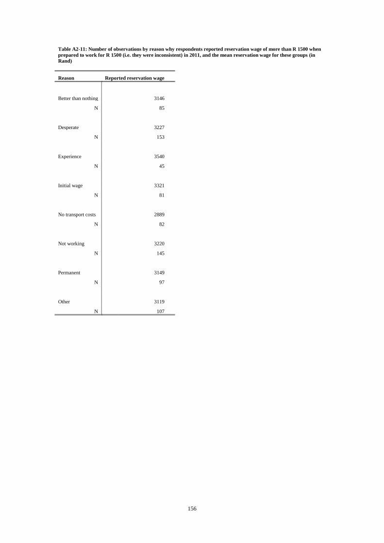
156

Table A2-11: Number of observations by reason why respondents reported reservation wage of more than R 1500 when

prepared to work for R 1500 (i.e. they were inconsistent) in 2011, and the mean reservation wage for these groups (in

Rand)

Reason Reported reservation wage

Better than nothing

3146

N

85

Desperate

3227

N

153

Experience

3540

N

45

Initial wage

3321

N

81

No transport costs

2889

N

82

Not working

3220

N

145

Permanent

3149

N

97

Other

3119

N

107

157

Figure A2-1: Distribution of reported reservation wages (natural log) for each of the six enumerators the respondent was

initially assigned to (randomly) in Gauteng and Limpopo (Epanechnikov kernel function)

0.5

11

.5

6 7 8 9 10 11 6 7 8 9 10 11

Gauteng Limpopo

One Two Three

Four Five Six

Reported Reservation Wage

Graphs by Province respondent was sampled in

158

This page is intentionally left blank.

159

Chapter 3. Are young South Africans overly optimistic about

their labour market prospects?

“I didn’t struggle to be poor” – Power 98.7 FM billboard on the M1 De Villiers Graaff

motorway, a few kilometres before the Sunbird e-toll gantry (coming from Pretoria)

Abstract

In this chapter we investigate whether young workers in South Africa are unaware that they

are optimistic about their labour market prospects. Expectations play a key role in job search

theory and we find that a portion of young South Africans may be optimistic about the wage-

offers they believe they will receive even though unemployment is pervasive among youth in

South Africa. Importantly a large proportion of the young South Africans in our sample

remain relatively optimistic when they are given reliable information about the dire

employment prospects of their peers, and there is an inverse association between remaining

optimistic and subsequent employment. We also find that giving a group of young South

Africans more reliable information about their employment prospects has no effect on their

labour markets outcomes or their reported reservation wages one year later. Together these

results lead us to conclude that these young South Africans may be unaware that they are

optimistic about their labour market prospects and that these optimistic young South Africans

will likely be disappointed.

Acknowledgements

I would like to thank Linda and Ian for the discussions we had about Kruger and Dunning

(1999). I would also like to thank Justin Kruger for his assistance.

160

Introduction

In the previous chapter we find that despite the high levels of unemployment among youth in

South Africa there is a large difference between the reported reservation wages and the

minimum wage offer that young workers in South Africa report they will accept if they were

desperate for a job. One reason for this is the reported reservation wages of unemployed

youth in South Africa are higher than what they could reasonably expect to earn because

many unemployed youth only have limited information on the labour market (Kingdon and

Knight, 2001). It is however unclear why these young workers do not revise their reported

reservation wages downward when they are confronted with unemployment. Similarly, why

do employed youth also report reservation wages that are higher than what they are earning?

Diagne and Irene (2009) also point out that African South African youth are relatively

optimistic about their labour market prospects. How do we reconcile the optimism of many

young South Africans with the high levels of unemployment among youth in South Africa?

We propose that optimism among young South Africans may be related to their inability to

assess their value to firms even when they are given reliable information about their labour

market prospects.

Diagne and Irene (2009) establish that changes in the job search status, search intensity and

reservation wages of youth in South Africa are related to changes in their subjective beliefs.

In this chapter we show that a large proportion of young South Africans report that they are

optimistic38 in terms of how likely it is that they will receive relatively high wage offers, even

after they are given reliable information about the dire labour market prospects of their peers.

Further, while employed young South Africans are more likely to be optimistic, these

relatively optimistic employed youth are also more likely to lose or leave jobs than their less

optimistic peers.

38 In this chapter we define optimism as positive bias in the assessment of the true probability of an outcome (an

event in space-time), and we regard optimism as a necessary condition for confidence.

161

In this paper we also show that giving a group of young South Africans aged 22 to 26

information on the wage offer prospects of their peers has no effect on their subsequent

labour market outcomes (including their reported reservation wages) one year later. The

results we present in this chapter consequently suggest that the assumptions in many job

search models, including that representative agents are certain about their relative ability and

update their expectations when they receive better information (see Rogerson, Shimer, and

Wright, 2004; and Eckstein and Van den Berg, 2007 for an overview of the job search

literature), may not be appropriate for South African youth (for a recent application see

Levinsohn and Pugatch, 2014). Our research is, to the best of our knowledge, the first to

frame the behaviour of unemployed youth in South Africa as a departure from some of the

assumptions that support these models. This is surprising since Beaulier and Caplan (2007:1)

argue the poor “deviate from the rational actor model to an unusually high degree.” Babcock,

Congdon, Katz and Mullainathan (2012: 1) also point out that “insights from behavioral

economics, which allow for realistic deviations from standard economic assumptions about

behavior, have consequences for the design and functioning of labor market policies.”

This chapter proceeds as follows. First we briefly outline the literature on type uncertainty

and optimism in job search. After this we present the data we use to demonstrate that young

South Africans may be optimistic about their labour market outcomes, the econometric

approach we use to show that this optimism is not necessarily associated with higher levels of

employment and earnings, and the results from our estimates which demonstrate that many of

the young South Africans in our sample may be unaware that they are optimistic about their

labour market prospects. We conclude with a discussion of these results and their implication

for policy-makers.

162

Type uncertainty and optimism

Traditional neoclassical labour market models predict that the amount of labour that workers

supply should equal the amount of labour demanded by firms at the equilibrium wage

(Eckstein and van den Berg, 2007). These models imply that youth unemployment in South

Africa is either voluntary or that employment is inhibited by minimum-wage regulation. An

alternate explanation for the high level of youth unemployment in South Africa, among others

(see Banerjee, Galiani, Levinsohn, McLaren, and Woolard, 2008), is that search frictions arise

as a consequence of imperfect information – both from the perspective of the person

searching for a vacancy and from that of the firm looking to fill a vacancy (Eckstein and Van

den Beg, 2007). This imperfect information (from the perspective of workers) generally refers

to uncertainty regarding market conditions such as the shape of the wage offer distribution

(Falke, Huffman, and Sande, 2006 a).

Falk, Huffman, and Sunde (2006 a: i) show though that while “standard search theory

assumes that individuals know, with certainty, how they compare to competing searchers in

terms of ability” many searchers are unaware of their relative ability. Falk, Huffman, and

Sunde (2006 b: i) develop an equilibrium search model with type uncertainty and non-

participation where “unsuccessful search induces individuals to revise their beliefs

downwards.” This model offers both a theoretical framework and another explanation for

why the unemployed youth in South Africa have reservation wages that are higher than what

they could reasonably expect to earn in employment. The dynamics in their model imply,

however, that there is a “declining hazard from unemployment to employment, arising due to

erosion of self-confidence in search”, since “search outcomes are only a noisy signal about

ability, some individuals can become overly discouraged and stop search too early due to

wrong beliefs”, and that “workers with greater unemployment duration are less confident, and

thus have a worse threat point in wage bargaining, consequently they earn lower starting

wages even if they are identical in terms of their productivity.” Further, even though they

163

relax the assumption that workers are certain about their type, these workers should update

their beliefs when they are given better information. They are nevertheless unable to

investigate the impact of unemployment on subjective beliefs in the field since this would

“require a survey that elicits individual’s beliefs about their relative abilities and job-finding

chances, and their certainty about these beliefs… which is currently unavailable” (Falk,

Huffman, and Sande, 2006 b: 28).

In Falk, Huffman, and Sunde (2006 a) they find (in a laboratory experiment) that people do

not fully update this assessment in a manner that would be consistent with Bayes’ law. Falk et

al. (2006 a) suggest this happens because people find it uncomfortable to receive negative

information about their relative ability. Further, since their equilibrium search model with

type uncertainty does not allow workers to have a preference for positive beliefs, it is also at

odds with the psychology literature where there is evidence that people are generally

overoptimistic about future life events (Van den Steen, 2004). Indeed Johnson and Fowler

(2011: 317) argue that “confidence is an essential ingredient in a wide range of domains

ranging from job performance and mental health to sports, business and combat”, and that it

may even be that “not just confidence but overconfidence – believing that you are better than

you are in reality – is advantageous because it serves to increase ambition, morale, resolve,

persistence or the credibility of bluffing, generating a self-fulfilling prophecy in which

exaggerated confidence actually increases the probability of success.”

Santos-Pinto and Sobel (2005) reason though that even if over-optimism is widespread it does

not constitute a compelling reason to amend modelling approaches. As Van den Steen (2004)

demonstrates rational agents with different priors tend to be overoptimistic about their

chances of success. If individuals make random errors in their subjective assessment of the

probability of success associated with an action, and they generally select the action they

believe offers them the highest probability of success, they are more likely to select actions

where they overestimated the probability of success associated with these actions and are

consequently optimistic about the probability of success. Santos-Pinto and Sobel (2005)

164

propose a similar mechanism to describe individuals’ positive self-image in subjective

assessments of their relative ability. They also permit individuals to have different skill

endowments and this allows them to model negative self-image. Nonetheless Santos-Pinto

and Sobel (2005) acknowledge that modifying beliefs by suppressing negative signals and

overemphasizing positive signals is outside of their framework. This is an important

constraint because, as Kahneman (2003) points out, people often act intuitively. Crucially,

“findings about the role of optimism in risk-taking, the effects of emotion in decision weights,

and fear in predictions of harm,” amongst others, “all indicate that the traditional separation

between belief and preference in analyses of decision making is psychologically unrealistic”

Kahneman (2003: 1470).

Rabin39 (1998: 26) outlines a growing literature which suggests that “once forming strong

hypotheses, people are often too inattentive to new information contradicting their

hypotheses.” An important feature of this confirmatory bias is that people do not only

misinterpret additional evidence but they also tend to use this misread evidence as additional

support for their initial belief. Further, Kruger and Dunning (1999) propose that people that

are not able to gauge their skill in a particular domain may have inflated self-assessments

because they are unable to evaluate competence in this domain. They suggest that people that

overestimate their ability within a particular domain suffer from a dual burden: “not only do

these people reach erroneous conclusions, and make unfortunate choices, but their

incompetence robs them of the metacognitive ability to realize it.” (Kruger and Dunning,

1999: 1121)

It is important to note that Kruger and Dunning (1999: 1122) define incompetence as “a

matter of degree and not one of absolutes”, and that “there is no categorical bright line that

separates competent individuals from incompetent ones”. Thus when they speak of

39 Rabin (1998) provides an excellent overview of “Psychology and Economics”. Rabin (2013:1) also explores

“the potential for using neoclassical (broadly defined) optimization models to integrate insights from psychology

on the limits to rationality into economics.”

165

"incompetent" individuals they mean people who are less competent than their peers. They

make “no claim that they would be incompetent in any other domains”.

Kruger and Dunning test four predictions. The first is that unskilled individuals will,

compared with their more skilled peers, overestimate their performance relative to objective

criteria. Second they will be less able than their more skilled peers to recognize competence

when they see it—“be it their own or anyone else's.” Third, unskilled individuals “will be less

able than their more competent peers to gain insight into their true level of performance by

means of social comparison information,” and they will therefore be “unable to use

information about the choices and performances of others to form more accurate impressions

of their own ability.” Finally unskilled individuals “can gain insight about their shortcomings,

but this comes (paradoxically) by making them more competent, thus providing them the

metacognitive skills necessary to be able to realize that they have performed poorly.”

Schlösser, Dunning, Johnson, and Kruger (2013) note that “such a pattern of gross self-

overestimation extends to real world settings, such as students taking classroom exams

(Dunning et al., 2003, Ehrlinger et al., 2008 & Ferraro, 2010), competitors engaged in

debate tournaments (Ehrlinger et al., 2008), lab technicians quizzed about everyday work

tasks and knowledge (Haun, Zeringue, Leach, & Foley, 2000), [and] players at chess

tournaments (Park & Santos-Pinto, 2010).”

South African youth may overestimate their labour market prospects because they are unable

to recognize competence (from the perhaps biased perspective of firms) and they are unable

to gain insight into their estimates using social comparison information. Furthermore there are

a number of settings where optimism could contribute to unemployment40. Dohmen (2014)

40 This optimism may – as Johnson and Fowler (2011: 317) suggest – lead to “hazardous decisions.” For example,

Dewing, Mathews, Fatti, Grimwood, and Boulle (2014: 64) point out that “retention in South Africa’s national

ARV treatment programme (the largest in the world) has deteriorated over time and as more people have been

enrolled in care.”

166

outlines the literature on such “nonstandard” beliefs in labour economics. This includes

Spinnewijn (forthcoming) who finds evidence that optimistic individuals may pursue search

strategies that are sub-optimal. Optimism may also lead workers to search (and apply) for the

types of jobs where there is no reasonable chance of success. Groh, McKenzie, Shammout

and Vishwanath (2014) show that unemployed Jordanian youth are more likely to apply for

jobs with higher prestige and are less likely to show up for interviews scheduled for low

prestige jobs. Young South Africans may also shirk on or leave jobs because they believe

they are under-valued in this employment. Similarly firms may be less inclined to employ and

train (or to continue to employ) relatively unskilled workers that are overly optimistic about

their employment prospects elsewhere. Another concern is that young workers that are

unaware that they are unskilled could become disillusioned.

Heine and Lehman (1995) find though that there is cultural variation in unrealistic optimism.

More importantly Ackerman, Beier and Bowen (2002), Krueger and Mueller (2002), and

Burson, Larrick and Klayman (2006) argue that, in certain situations, “regression to the mean,

coupled with the above average effect, would produce the basic relationship between

objective performance and self-perception attributed to the Dunning–Kruger effect”

(Schlösser et al., 2013: 86-87). Krajč and Ortmann (2008) also point out that the poorest

performers are more likely to be optimistic because they may only be able to make errors that

are positive.

167

The data

We investigate the relationship between optimism and outcomes in the labour market for

South African youth using the same dataset we used in the previous chapter. The Labour

Market Entry Survey (LME) was, as mentioned, conducted as part of a randomized control

trial (RCT) used to assess the impact of a wage subsidy voucher on the employment outcomes

of young African South Africans aged 20 to 24 (when the respondents were first interviewed

in 2009). The survey was conducted telephonically in 2011 using Computer-Assisted

Personal Interviewing software, and there were six enumerators. They were assigned

randomly to these six enumerators (in a random order), for each separate province. We first

surveyed the respondents who we had initially sampled in Gauteng. After this we surveyed

the respondents from Limpopo, and after Limpopo the respondents from KwaZulu-Natal.

Two enumerators stopped working before the survey ended and were replaced by two others.

In 2012 the respondents were interviewed for a fourth and final time. The surveys were again

allocated randomly in 2012, although they were not assigned to particular enumerators (the

follow-up surveys were assigned randomly to pages, in a random order, and these were then

allocated by the team-leader to the enumerators). There were seven enumerators in 2012 (this

includes the team-leader who completed a small number of the surveys that were still

outstanding towards the end of the survey).

In all of the LMES waves (from 2009 to 2012) the respondents were asked “What is the

MINIMUM MONTHLY wage you are prepared to work eight hours a day five days a week

for?” We will again refer to this as the reported reservation wage. In the previous chapter we

show that this measure of the reservation wage is exposed to considerable measurement error.

For the employed it is, on average, significantly more than what they are earning. It is also

significantly larger, on average, than what the unemployed and employed respondents said

they would be prepared to work for if they were desperate for a job (We asked the

168

respondents “What is the MINIMUM MONTHLY wage you are prepared to work eight hours

a day five days a week for if you were desperate for a job?)

In 2011 we added the following question to the survey after we asked the respondents for

their reservation wage: How good do you think your chances are of finding any

PERMANENT FULL-TIME job in the NEXT 3 months that PAYS R {reported reservation

wage multiplied by 1.3} A MONTH, if you wanted such a job? Thus, if the respondent had

answered R3500 (the sample median in 201141) to the question “What is the MINIMUM

MONTHLY wage you are prepared to work eight hours a day five days a week for?” the

respondents would have been asked “How good do you think your chances are of finding any

PERMANENT FULL-TIME job in the NEXT 3 months that PAYS R4450 A MONTH, if you

wanted such a job?” The respondents were given the following answers to choose from

“VERY high (VERY good); high (good); average (neutral/neither good nor poor/50-50); low

(poor/bad); VERY low (VERY poor/VERY bad).” We will refer to this as the respondent’s

initial optimism, and we expect the respondents to be optimistic because many of the

respondents are likely to have only limited information on their labour market prospects. The

respondents were then asked “How good do you think YOUR chances of finding SUCH a

permanent full-time job are when COMPARED to other young people who LIVE IN THE

SAME AREA as you, if you wanted such a job?” and could choose from “Much better (much

higher); better (higher); the same (neutral/50-50); worse (lower); much worse (much lower).”

After this the respondents were told "Wits University research shows that the chances of

young people with the same education as you and living in your area finding SUCH work in

the next 3 months are VERY low (VERY poor/VERY bad)" and asked if they understood (or

disagreed, the question was open-ended) with the statement. We then asked the respondents:

“NOW that I have told you this, how good do you think your chances are of finding any

permanent full-time job in the next three months that PAYS R {reported reservation wage

41 In comparison the median earnings of the employed in 2011 were R 2400 per month. The minimum wage was

approximately R 1500.

169

multiplied by 1.3} a month, if you wanted such a job?” and presented them with the same set

of answers to the original question. In this chapter we will refer to this as the respondent’s

optimism.

The respondents had been part of this Wits University study for two years (i.e. they had been

interviewed twice before) by the time they were asked this question and we are unable to

think of a reason why the respondents would doubt the authority of the statement. Regardless,

this is not concern to us because we expect those respondents that are optimistic to disagree

(particularly when this optimism is related to their inability to recognize ‘competence’ in the

labour market). Only 20% of the respondents indicated that they did not agree with this

statement when we asked them “Does the respondent understand the statement?” They could

choose “The respondent understands”, “The respondent does not agree”, or they could

provide their own response (which we coded in those cases where this response suggested

they did not agree). Further we asked the respondents why they had (or had not) changed their

answer after the enumerator had told them about this research. They could respond “He/she

believes the Wits University research”, “He/she does not think the research applies to

him/her”, “He/She does not believe the Wits University research”, or define their response

(which we also coded). Approximately six percent of the respondents indicated that they did

not believe the Wits University research.

We set the hypothetical wage-offer to 130% of their reservation wage to make the probability

of receiving this wage offer as low as possible without making it appear completely

implausible (to us at least). Furthermore, at the time we knew that only a very small number

of the respondents that were unemployed would receive a permanent offer within three

months because employers are granted a probation period that is only restricted to be of a

reasonable duration. Thus anyone that provided an answer other than “Very low” is optimistic

to varying degrees and relatively optimistic in terms of their labour market prospects when

compared to the prospects of the “other young people” that are the subject of the statement.

We will henceforth regard those individuals who responded “Low” as a little optimistic, those

170

that respondent “Average” as moderately optimistic, those that respondent “High” as very

optimistic, and those respondents that answered “Very high” as extremely optimistic.

We did not want to discourage anyone which is why we relate the ‘evidence’ to the

circumstances of other young people and we set the minimum offer to R1950 for those

respondents who reported reservation wages that were less than R1500. This is also why we

use the vague references “young” and “area” when we frame the range of social comparison

information. The purpose of these qualifications is merely to restrict the comparison to people

within the respondent’s more immediate frame of reference. This will naturally depend on the

respondent. Further, to make sure that we had not discouraged the respondents, we also

randomly skipped over the statement (and corresponding question) for (in expectation) half of

the respondents in KwaZulu-Natal.

As with the reported reservation wage, the data we collect may be sensitive to interpretation

and other forms of measurement error (in addition to the more immediate concern that the

reported optimism does not reflect what the respondent genuinely believes). For example, it is

unclear why one fifth of the respondents initially told us that they did not agree with the

statement and only six percent told us that they did not believe the research after we asked

them for their revised expectation of receiving the hypothetical offer after the statement. One

explanation is the substantial variation in the answers to this question (and other questions)

between the groups of respondents that were randomly assigned to different enumerators in

2011. Table A3-1 in the Appendix presents an overview of the assignment and the allocation,

and Table A3-3 shows the disparity in optimism between the groups of respondents that were

initially assigned to each of the six enumerators at the start of the survey (even though they

were balanced in 2011 in terms of the characteristics they reported in 2010). This is also one

of the reasons why the respondents in KwaZulu-Natal were less likely to be optimistic than

those in the other provinces (in 2011 two of the enumerators were replaced by two new

enumerators for the survey of the respondents that were initially sampled in KwaZulu-Natal).

171

At least some of this variation can be explained by the differences in the reported reservation

wages between enumerators (that were highlighted in the previous chapter). There was one

enumerator (who we refer to as Enumerator Six, of the initial six) in particular that recorded a

significantly different reservation wage distribution for the respondents that were assigned to

this enumerator from both Gauteng and in Limpopo42.

The variation between the surveys that were initially assigned to one of the six enumerators

also extends to the other outcomes of interest to this chapter. For example, the respondents

were asked, “How happy are you with your life in general?” and could choose from, in this

order, “Very happy; happy; neither happy or unhappy; unhappy; and very unhappy”. Those

respondents Enumerator Six interviewed were less likely to be happy, by this measure, in

both 2011 and, oddly, in 2012. They were also significantly less likely to include “Income

from working for someone else” and more likely to include “Income from piece/odd jobs”

among the answers to the question “How do you support yourself?” This may explain why

they, on average, reportedly earned less in 2012 than their counterparts (that were assigned to

other enumerators in 2011) but there are no differences between these groups in the value of

support they get from all sources (which includes grants, and transfers from family and

friends etc.). The latter was asked before the respondents were given the information about

the prospects of their peers and then asked to assess their prospects, while we measure the

former based on the question “How much money did you take home in the last month doing

this wage-job?” and “How much money did you take home in the last month working in self-

employment?” These two questions were presented to the respondents after they were given

the information about the prospects of their peers and had, in separate questions just prior to

each of these earnings questions, indicated that they had done at least some work for anyone

else or themselves in the month preceding the interview (those that had not were asked if they

had ever worked in these forms of employment and what they were earning in the last month

42 Enumerator Six was the most experienced enumerator in the team and left, rather unexpectedly, before we

started the KwaZulu-Natal survey in 2011.

172

of this employment, and we set earnings to zero for these workers and those that had never

had a job or worked for themselves). While a significant proportion of the respondents that

subsequently reported they were working for someone else or they were self-employed in

2012 had not listed “Income from working for someone” or “Income from self-employment”

among the ways that they support themselves, none of the respondents that were interviewed

by Enumerator Six in 2011 were inconsistent in this regard in 2012.

We can only speculate on the cause of the differences in both 2011 and 2012 between those

respondents that were assigned to Enumerator Six and those that were initially assigned to the

other five enumerators in 2011 (or the other differences between the responses of the

respondents assigned to enumerators one through to five). There are no statistically

significant differences in the duration of the interviews in 2011 between any of enumerators,

though. We will include the initial assignment to the enumerators (which is, as mentioned,

random) in our econometric specification so that, we hope, we will reduce any bias associated

with this assignment. Further, after the interview we asked the enumerators how honest the

respondent was (Completely honest; mostly honest; sometime honest and sometimes

dishonest, mostly dishonest and completely dishonest). Even though more than 80% were

“Mostly honest” or “Completely honest” in both rounds, there is a significant regression to

“Mostly honest” in 2012 from “Completely honest” in 2011. We will exclude those

respondents that were mostly or completely dishonest from the subsequent analysis, and as

we explain in the next section, we will include this impression (completely honest; mostly

honest; or sometime honest and sometimes dishonest) in our econometric specification43.

43 Coincidently the respondents that were interviewed by Enumerator Six were (by this enumerator’s assessment)

significantly more likely to be “Completely honest” than those respondents that were interviewed by the other

enumerators. It is unlikely that Enumerator Six was assigned two independent random samples that happened to be

populated by this type (or were more likely to be selected), although we find that this difference persists into 2012

for both Gauteng and Limpopo (Enumerator Six was not part of the 2012 survey where the survey-responses were,

as mentioned, again randomly allocated among the new set of enumerators). We were consequently concerned to

find that those respondents in both Gauteng and Limpopo that had been assigned to Enumerator Six were also

173

These perceptions are of course subjective and it is difficult to determine if they are related to

the enumerator. Nevertheless they suggest that we should interpret the responses of the

‘dishonest’ respondents with caution and that at least some of the variation we observe may

reflect the respondents’ levels of engagement with the survey. We also asked the enumerator

how well the respondent spoke English44 (very poorly, poorly, average, well, or very well)

and we will include this measure in the econometric specification we outline in the next

section. This is also subjective assessment. However the enumerators were instructed to

translate the questions from English and this question therefore reflects the level of translation

that was required for the particular interview.

The following table (Table 3-1) presents the number of observations in each period (2011 and

2012) by the province the respondent was initially sampled in (in 2009). We, as mentioned,

exclude those respondents that were deemed “Completely dishonest” and “Mostly dishonest”.

Further, we exclude those respondents that have missing earnings information in 2011 or

2012 and those that are younger than 22 or older than 27 in 2011 (because they are outliers).

In the balanced panel we also exclude those respondents who told us in 2011 they would not

be prepared to start within a week even if they were offered a suitable job, and those

respondents that classified themselves as “not economically active” in 2011. These

respondents are excluded because we believe their assessments (at least in 2011) are more

significantly less likely to be employed (When we asked the respondents “What activity currently takes up most of

your time?”) in 2012 than those respondents who had been assigned (initially) to other enumerators in 2011, even

after we control for selection (we estimate the effect on employment using several approaches, including fixed-

effects specifications and a specification where we model selection into the 2014 survey by using the order that the

survey response was assigned to the enumerators in 2012 as an exclusion restriction). Upon further investigation

we discovered something even more remarkable: the respondents Enumerator Six interviewed in 2011 were

significantly more likely to be regarded as honest in 2012 (across Gauteng and Limpopo, by a different set of

enumerators – when we use an ordered probit specification).

44 The enumerators, who are multilingual, conducted the interview in the respondent’s preferred language. There

were a small number of surveys where one of the enumerators (who was more comfortable conversing in Venda)

had to take over from the other enumerators.

174

likely to be hypothetical and less likely to be have an effect on their behaviour. Consequently

the sample is informative about the young South Africans in our sample that, by their

admission, would consider a job offer.

The treatment group in Table 3-1 are those respondents in KwaZulu-Natal that were given the

information about the prospects of their peers. The control group are those respondents that

were not given this information. The large difference in the number of balanced panel

observations in KwaZulu-Natal is due to the 205 observations that serve as the control when

we test the effect of giving young people this information. We do not exclude any of the

observations (other than those that attrite) in this trial because the characteristics of the

individuals are, by construction, orthogonal to treatment status.

Table A3-2 in the Appendix presents a comparison of the respondents that are excluded, by

gender, age, education, and the primary activity the respondent was engaged in, in 2011 (the

primary activity refers to the activity that currently takes up most of the respondent’s time).

The sample is, as we mentioned in the previous chapter, not representative of young South

Africans. In particular the vast majority of the respondents had a Matric and a large

proportion indicated that they had a “Certificate” when we asked them if they had any further

education. However only a third listed “Working for someone else” as the activity that takes

up most of their time.

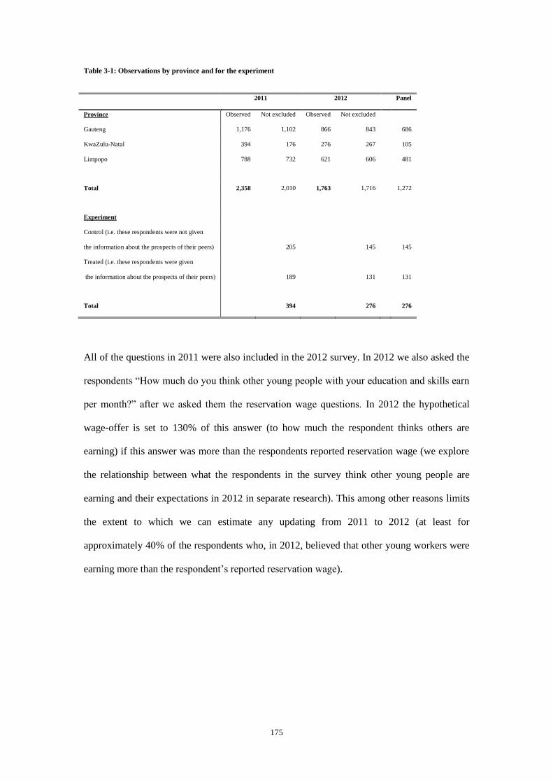
175

Table 3-1: Observations by province and for the experiment

2011 2012

Panel

Province Observed Not excluded Observed Not excluded

Gauteng 1,176 1,102 866 843

686

KwaZulu-Natal 394 176 276 267

105

Limpopo 788 732 621 606

481

Total 2,358 2,010 1,763 1,716

1,272

Experiment

Control (i.e. these respondents were not given

the information about the prospects of their peers)

205

145

145

Treated (i.e. these respondents were given

the information about the prospects of their peers)

189

131

131

Total

394

276

276

All of the questions in 2011 were also included in the 2012 survey. In 2012 we also asked the

respondents “How much do you think other young people with your education and skills earn

per month?” after we asked them the reservation wage questions. In 2012 the hypothetical

wage-offer is set to 130% of this answer (to how much the respondent thinks others are

earning) if this answer was more than the respondents reported reservation wage (we explore

the relationship between what the respondents in the survey think other young people are

earning and their expectations in 2012 in separate research). This among other reasons limits

the extent to which we can estimate any updating from 2011 to 2012 (at least for

approximately 40% of the respondents who, in 2012, believed that other young workers were

earning more than the respondent’s reported reservation wage).

176

Descriptions of the data

In this chapter we will refer to four different measures of employment. Those respondents

that did any work for someone else in the past month had a job. The respondents that had a

job or were self-employed had work (which we will refer to as “Any work”). Those that listed

“Working for someone else” as their main activity are wage-employed. Finally those that

described themselves as employed are the self-reported employed. These groups are not

mutually exclusive. For example, some of the respondents that indicated that they had done

any work (i.e. they had a job or had done some work for themselves in the past month) did

not indicate, when we asked them what their main activity was, that they were working for

someone else (i.e. they were, by our definition, employed) or working for themselves

(similarly, some that answered that they were working for someone else or working for

themselves did not indicate that they had done any work in the past month). Further, some of

the respondents that had done any work and indicated that their main activity was working for

someone else did not regard themselves as employed (i.e. when we asked them what they

regarded their state as they did answer “Employed”). Roberts and Schöer (ongoing) explore

the relationship between these different measures of employment in separate research. We use

the different measures here to demonstrate that the results are robust across these measures.

The unemployed are those that listed their main activity as “Unemployed and searching for

work”, and the self-reported unemployed are the respondents who told us they defined

themselves as either “Unemployed and looking for work” or “Unemployed, I want work but I

am not looking for work”. The ‘discouraged’ are the unemployed or self-reported

unemployed that had not actively searched for work in the past month. This includes a large

proportion of the respondents who indicated that they were “Unemployed and looking for

work” but had not searched for work in the past week.

We will use two measures of earnings. As mentioned we asked the respondents “How much

money did you take home in the last month doing this wage-job?” and “How much money did

177

you take home in the last month working in self-employment?” To calculate earnings we add

the answers (which are zero for those that did not do any work) to these two questions. Prior

to this we had asked the respondents how they supported themselves and “How much do you

get per month (including income, value of gifts, food etc.)?” which we will refer to as their

income. We also compute an alternate measure of earnings by replacing reported earnings

with income when the former is larger than the latter.

The following tables (Table 3-2 through to Table 3-7) provide an overview of the data. There

is variation between the outcomes of those respondents who answered “Low”, “Average”,

“High” and “Very high” in the tables we outline in this section. However the objective of the

analysis is to investigate the relationship between being optimistic and labour market

outcomes. While it would be appealing to look for evidence of Bayesian-type updating we

cannot think of a reason why this would influence the conclusions of this chapter. Another

reason such an approach is not warranted is because we do not attach probabilities to the

answers for these questions. It also turns out that, as we will discuss when we present the

result, the outcomes of the individuals within the optimistic group (“Low” to “Very high”) are

more alike than they are when compared to those individuals that are not optimistic (“Very

low”). Recall that any respondent who answered “Low” is relatively optimistic compared to

other young people who, we told them, had a “VERY low” chance of finding such a job. We

will as mentioned also present evidence from the experiment which finds that telling the

respondents “"Wits University research shows that the chances of young people with the same

education as you and living in your area finding SUCH work in the next 3 months are VERY

low (VERY poor/VERY bad)" no effect on the outcomes we have described in this section.

Table 3-2 reports the percentage of respondents by their response to the question “How good

do you think your chances are…?”, both before (i.e. initial optimism) and after (i.e. optimism)

we tell the respondents "Wits University research shows that the chances of young people

with the same education as you and living in your area finding SUCH work in the next 3

178

months are VERY low (VERY poor/VERY bad)". Fewer than 20% of the respondents in the

sample initially thought their chances of finding such jobs are very low.

Table 3-3 also shows that while many of the respondents update their assessment, only a

small proportion (less than 30%) respond “Very low”. Some even update in the other

direction. Most of the respondents maintain their initial assessment even though the majority

of the respondents told us they had or had not changed their answer because they believe the

research (Table 3-4). One reason for this perhaps is that as we show in Table 3-5 and Table 3-

6 the respondents who did not answer “Very low” after the statement were more likely (in

2011) to be employed, and less likely to be unemployed, than those that acknowledged that

their chances may be very low. Importantly, while they had more income, there does not

appear to be any systematic difference in their reservation wages. In Table 3-6 we see that the

median reported reservation wage of all of these groups are higher than the median wages of

those that had a job (R 2400), and significantly higher than the earnings and income of the

respondents.

In Table 3-7 we show that at most 6% of the young people in the sample we use were earning

more in 2012 than the hypothetical offer that we had presented in 2011. This is the case for

both those respondents that answered “Very low”, and those that we regard as optimistic (the

difference between these two groups is not statistically significant). Table 3-8 shows that the

respondents that were optimistic in 2011 were more likely to be employed, less likely to be in

jobs in which they were unhappy or very unhappy, and more likely to feel “Very happy” or

“Happy” with their lives in general in 2011. This gap appears to narrow in 2012 though. One

reason for this is that as we show in Table 3-9 a higher percentage of the respondents that

were optimistic in 2011 transitioned out of wage-employment in 2011 into unemployment in

2012 (we use the primary activity because this is the only classification of the labour market

states that is mutually exclusive).

179

Table 3-2: Percentage of respondents by level of optimism

Initial optimism in 2011 Optimism in 2011

Not

optimistic

(Very low)

A

little

optimistic

(Low)

Moderately

optimistic

(Average)

Very

optimistic

(High)

Extremely

optimistic

(Very high)

Not

optimistic

(Very low)

A

little

optimistic

(Low)

Moderately

optimistic

(Average)

Very

optimistic

(High)

Extremely

optimistic

(Very high)

Province

Gauteng 18 24 26 26 7 28 25 19 24 4

KwaZulu-

Natal 23 29 24 19 6 34 32 17 11 5

Limpopo 18 19 28 28 7 26 22 23 25 5

Gender

Male 23 23 26 23 6 29 22 21 23 4

Female 16 22 27 28 7 27 26 20 23 5

Age

22 20 20 28 22 10 27 26 22 19 6

23 19 22 25 27 7 28 23 20 26 4

24 16 26 26 29 3 23 28 21 25 4

25 16 23 31 23 6 27 26 19 23 5

26 22 20 22 27 9 32 21 21 23 4

27 22 16 28 26 8 30 23 20 22 5

Total 19 22 26 26 7 28 25 20 23 4

The table suggests that the majority of the respondents in your survey were relatively optimistic (they did not respond “Very

low”) about their labour market prospect both before and after we told the respondents that the prospects of their peers finding

jobs that paid 130% of their reported reservation wage were VERY low.

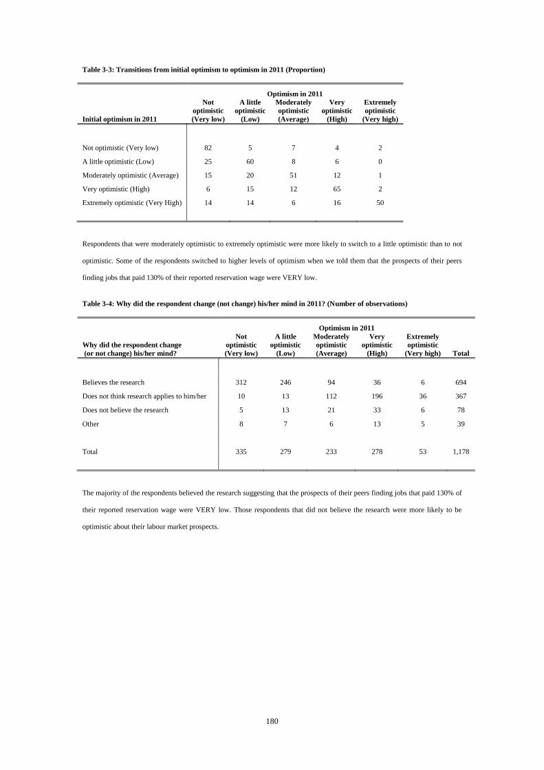
180

Table 3-3: Transitions from initial optimism to optimism in 2011 (Proportion)

Optimism in 2011

Initial optimism in 2011

Not

optimistic

(Very low)

A little

optimistic

(Low)

Moderately

optimistic

(Average)

Very

optimistic

(High)

Extremely

optimistic

(Very high)

Not optimistic (Very low) 82 5 7 4 2

A little optimistic (Low) 25 60 8 6 0

Moderately optimistic (Average) 15 20 51 12 1

Very optimistic (High) 6 15 12 65 2

Extremely optimistic (Very High) 14 14 6 16 50

Respondents that were moderately optimistic to extremely optimistic were more likely to switch to a little optimistic than to not

optimistic. Some of the respondents switched to higher levels of optimism when we told them that the prospects of their peers

finding jobs that paid 130% of their reported reservation wage were VERY low.

Table 3-4: Why did the respondent change (not change) his/her mind in 2011? (Number of observations)

Optimism in 2011

Why did the respondent change

(or not change) his/her mind?

Not

optimistic

(Very low)

A little

optimistic

(Low)

Moderately

optimistic

(Average)

Very

optimistic

(High)

Extremely

optimistic

(Very high) Total

Believes the research 312 246 94 36 6 694

Does not think research applies to him/her 10 13 112 196 36 367

Does not believe the research 5 13 21 33 6 78

Other 8 7 6 13 5 39

Total 335 279 233 278 53 1,178

The majority of the respondents believed the research suggesting that the prospects of their peers finding jobs that paid 130% of

their reported reservation wage were VERY low. Those respondents that did not believe the research were more likely to be

optimistic about their labour market prospects.

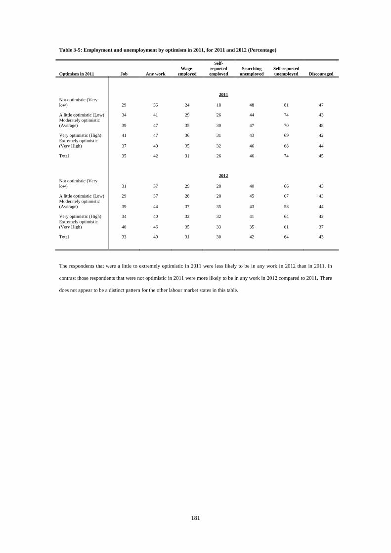
181

Table 3-5: Employment and unemployment by optimism in 2011, for 2011 and 2012 (Percentage)

Optimism in 2011 Job Any work

Wage-

employed

Self-

reported

employed

Searching

unemployed

Self-reported

unemployed Discouraged

2011

Not optimistic (Very

low) 29 35 24 18 48 81 47

A little optimistic (Low) 34 41 29 26 44 74 43

Moderately optimistic

(Average) 39 47 35 30 47 70 48

Very optimistic (High) 41 47 36 31 43 69 42

Extremely optimistic

(Very High) 37 49 35 32 46 68 44

Total 35 42 31 26 46 74 45

2012

Not optimistic (Very

low) 31 37 29 28 40 66 43

A little optimistic (Low) 29 37 28 28 45 67 43

Moderately optimistic

(Average) 39 44 37 35 43 58 44

Very optimistic (High) 34 40 32 32 41 64 42

Extremely optimistic

(Very High) 40 46 35 33 35 61 37

Total 33 40 31 30 42 64 43

The respondents that were a little to extremely optimistic in 2011 were less likely to be in any work in 2012 than in 2011. In

contrast those respondents that were not optimistic in 2011 were more likely to be in any work in 2012 compared to 2011. There

does not appear to be a distinct pattern for the other labour market states in this table.

182

Table 3-6: Income and Reservation Wages by optimism in 2011, for 2011 and 2012 (in Rand)

Optimism in 2011

Earnings

Earnings

(alternate

measure) Income Reservation wage

Reservation wage

if desperate

Difference

between

reservation wage

and earnings

2011

Not optimistic

(Very low)

Mean 828 629 1063 3903 1851 3075

Median 0 0 600 3500 1500 3000

A little optimistic

(Low)

Mean 924 730 1159 3959 1714 2999

Median 0 0 800 3500 1500 2700

Moderately

optimistic

(Average)

Mean 1219 947 1306 4123 1858 2709

Median 0 0 800 3500 1500 2500

Very optimistic

(High)

Mean 1105 891 1354 3968 1937 2808

Median 0 0 960 3500 1500 2500

Extremely

optimistic (Very

High)

Mean 1417 1130 1516 4454 2266 3037

Median 0 0 1000 3500 1500 2500

Total

Mean 1021 801 1223 4001 1858 2919

Median 0 0 800 3500 1500 2500

2012

Not optimistic

(Very low)

Mean 1100 719 1356 4332 1870 3168

Median 0 0 1000 3800 1500 3000

A little optimistic

(Low)

Mean 1062 599 1318 4264 1748 3193

Median 0 0 1000 3695 1500 3000

Moderately

optimistic

(Average)

Mean 1162 703 1450 4875 1958 3294

Median 0 0 970 4000 1500 3000

Very optimistic

(High)

Mean 1302 686 1343 4781 2059 3444

Median 0 0 1000 4000 1500 3000

Extremely

optimistic (Very

High)

Mean 1501 848 1338 4972 2183 3310

Median 0 0 800 3500 1500 3000

Total Mean 1168 684 1362 4558 1916 3270

Median 0 0 1000 4000 1500 3000

There does not appear to be a distinct pattern between income and reservation wages for the different levels of optimism.

183

Table 3-7: Difference between hypothetical offer in 2011 and earnings in 2012 by optimism in 2011 (in Rand)

Optimism in 2011

Hypothetical

offer (2011)

Difference

between

hypothetical

offer (2011)

and earnings

(2012)

Difference

between

hypothetical

offer (2011)

and earnings

(alternate

measure,

2012)

Percentage

earning more

(2012) than

hypothetical

offer (2011)

Percentage

earning more

(alternate

measure, 2012)

than

hypothetical

offer (2011)

Not optimistic Mean 5086 3899 4326 4% 1%

Percentile:

5 1950 340 1100

10 2340 1250 1950

25 3250 2350 2600

50 4550 3900 3900

75 6500 5200 5200

90 7800 6500 7450

95 10400 9100 10400

Optimistic Mean 5253 3886 4490 6% 1%

Percentile:

5 1950 -400 1250

10 2340 800 1950

25 3250 2050 2600

50 4550 3510 3900

75 6500 5200 5460

90 9100 7800 7800

95 11050 9100 9700

Total Mean 5207 3889 4445 6% 1%

Percentile:

5 1950 -300 1250

10 2340 920 1950

25 3250 2140 2600

50 4550 3640 3900

75 6500 5200 5300

90 8450 7400 7800

95 10400 9100 9750

Only four percent of the respondents that were not optimistic in 2011 and six percent of the respondents that were optimistic in

2011 were earning more in 2012 than the hypothetical offer that was made to them.

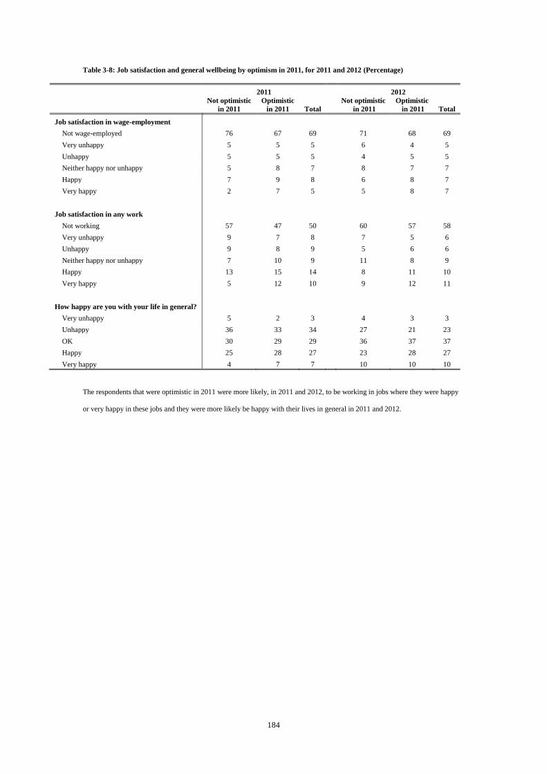
184

Table 3-8: Job satisfaction and general wellbeing by optimism in 2011, for 2011 and 2012 (Percentage)

2011

2012

Not optimistic

in 2011

Optimistic

in 2011 Total

Not optimistic

in 2011

Optimistic

in 2011 Total

Job satisfaction in wage-employment

Not wage-employed 76 67 69

71 68 69

Very unhappy 5 5 5

6 4 5

Unhappy 5 5 5

4 5 5

Neither happy nor unhappy 5 8 7

8 7 7

Happy 7 9 8

6 8 7

Very happy 2 7 5

5 8 7

Job satisfaction in any work

Not working 57 47 50

60 57 58

Very unhappy 9 7 8

7 5 6

Unhappy 9 8 9

5 6 6

Neither happy nor unhappy 7 10 9

11 8 9

Happy 13 15 14

8 11 10

Very happy 5 12 10

9 12 11

How happy are you with your life in general?

Very unhappy 5 2 3

4 3 3

Unhappy 36 33 34

27 21 23

OK 30 29 29

36 37 37

Happy 25 28 27

23 28 27

Very happy 4 7 7

10 10 10

The respondents that were optimistic in 2011 were more likely, in 2011 and 2012, to be working in jobs where they were happy

or very happy in these jobs and they were more likely be happy with their lives in general in 2011 and 2012.

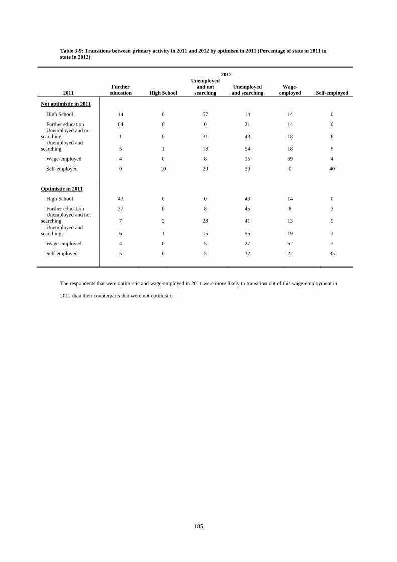
185

Table 3-9: Transitions between primary activity in 2011 and 2012 by optimism in 2011 (Percentage of state in 2011 in

state in 2012)

2012

2011

Further

education High School

Unemployed

and not

searching

Unemployed

and searching

Wage-

employed Self-employed

Not optimistic in 2011

High School 14 0 57 14 14 0

Further education 64 0 0 21 14 0

Unemployed and not searching 1 0 31 43 18 6

Unemployed and

searching 5 1 18 54 18 5

Wage-employed 4 0 8 15 69 4

Self-employed 0 10 20 30 0 40

Optimistic in 2011

High School 43 0 0 43 14 0

Further education 37 0 8 45 8 3 Unemployed and not

searching 7 2 28 41 13 9

Unemployed and searching 6 1 15 55 19 3

Wage-employed 4 0 5 27 62 2

Self-employed 5 0 5 32 22 35

The respondents that were optimistic and wage-employed in 2011 were more likely to transition out of this wage-employment in

2012 than their counterparts that were not optimistic.

186

The econometric approach

To investigate the extent to which there is an association between optimism (as we have

defined earlier) and labour market outcomes we use the following fixed-effects and

conditional logistic fixed-effects specifications for the continuous (𝑦𝑖𝑡, e.g. earnings), binary

(Chamberlain, 1980) or multinomial outcomes (𝑦𝑖𝑡∗ , e.g. employed; or one of employed,

unemployed or not economically active; Pforr, 2014) in 2011 (t = 1) and 2012 (t = 2):

𝑦𝑖,𝑡 𝑜𝑟 𝑦𝑖,𝑡∗ = 𝛽𝑘𝑖,2011 + 𝛾�⃗�𝑖,𝑡 + 𝑎𝑖 + 𝑢𝑖,𝑡 (1)

Here 𝑘𝑖,2011 takes on a value of one in 2012 if the respondent was optimistic in 2011 and zero

otherwise (i.e. it is set to zero in 2012 for those respondents that were not optimistic in 2011

and for all observations in period 2011).

�⃗�𝑖𝑡 includes the age (and age squared) of the respondent on the date of the interview (and

therefore includes the fraction of the year), the enumerator the respondent survey was initially

assigned to (e.g. Enumerator 2 in 2011, Enumerator 1 in 2012 etc.); whether the respondent

was “sometimes honest, sometimes dishonest”, “mostly honest”, or “completely honest”; and

how well the respondent spoke English (“Very poorly”, “poorly”, “average”, “well”, or “very

well”). 𝑎𝑖 is the individual fixed-effect. We include the enumerator, and their perceptions

about how honest the respondents was (and how well the respondent spoke English) to lessen

the bias associated with measurement error (since we are using a fixed effects specification

these measures are consequently a reflection of the enumerators as a group). The initial

assignment to the enumerator will also consequently capture period effects.

𝑘𝑖,2011 is the difference in the difference between those respondents that were optimistic and

those that were not optimistic in 2011:

𝐸[(𝑦𝑖,2012 − 𝑦𝑖,2011)| 𝑘𝑖,2011 = 1, �⃗�𝑖𝑡] − 𝐸[(𝑦𝑖,2012 − 𝑦𝑖,2011)| 𝑘𝑖,2011 = 0, �⃗�𝑖𝑡]

187

Kruger and Dunning (1999) argue that unskilled individuals are less likely to use information

and can only gain insights by becoming more skilled. This is why we estimate the fixed-effect

of this optimism in 201145 . It is unlikely that the two types of individuals would have

followed equivalent trends if we had been able to induce optimism46 and we are unable to

make any assumptions about the nature of these trends. Consequently, like Dunning and

Kruger (1999), we are only able to draw descriptive inferences about the differences in the

trends for these two groups of individuals. The purpose of this approach is merely to

determine if the relatively optimistic individuals were more likely to, as they expect, be

employed than their less optimistic counterparts in our sample (controlling for measurement

error and any differences in the age of the respondents).

Further, while 𝑎𝑖 should (we hope) reduce the bias associated with non-random attrition

among the sample in 2011 to 2012, we also estimate these specifications using inverse

probability weights. In our case the inverse probability weight (IPW) is based on the

following probit specification for the observations in 2011:

45 This is also why we (among other reasons) did not construct comparable measures of optimism across 2011 and

2012 for a large proportion of the sample. However, this would be the case even if we had used the same anchor

because the hypothetical offer is related to the respondent’s reservation wages and this may have changed over

these two periods. In hindsight a better approach would have been to use the hypothetical offer we made in 2011 in

the 2012 question so that we could explore e.g. how work experience and the duration in unemployment

(conditional on ai) are related to this assessment. Unfortunately at the time (2012) we were unaware that we had

made a poor call in this regard (among others).

46 It is similarly unlikely that we’ll ever be able to randomize ‘incompetence’ in the field. Further, it appears that a

laboratory setting would, at best, only allow us to demonstrate that the unskilled are unaware and that this has an

effect on the outcomes of the games the subjects are playing (perhaps by randomizing the level of training). We

were initially interested in testing if the treated respondents were less likely to be optimistic because they had more

experience (they were more likely to be employed) etc. We do not include the treatment status of the respondents

in this specification, though, because the treatment had been assigned in 2010 and there was no difference in the

level of optimism between the treatment and control groups in 2011. The direction of the point estimates in the

results we present in the next section correspond when we estimate (1) separately for these two groups, although

the two sub-samples are under-powered.

188

𝑛𝑜𝑖,2012∗ = 𝛾𝑝𝑖,2012 + 𝑢𝑖,2012 (2)

𝑛𝑜𝑖,2012 is one if the respondent is not observed in 2012 (because of attrition or non-response)

and zero otherwise. In 2012 we assigned the follow-up surveys to enumerators, randomly, by

page. 𝑝𝑖,2012 is a set of dummies for the date on which the page with the respondent’s details

was allocated to the enumerators. We attribute the difference in number of respondents that

were surveyed to the effort of the enumerators that had access to the pages on these dates (and

an error). Therefore we use the inverse of the probability of not being observed because this

gives more weight, on average, to those observations that were more likely to be observed

because of the effort of the enumerators to track them down.

The approach (i.e. weighting) we use does not consider the outcomes of those that would

never have participated in the 2012 survey-round regardless of the effort of the enumerators.

This is a concern if this group is, for example, more likely to be employed. There is, however,

data on the primary activity, age, honesty, how well the respondent spoke English, and the

assignment to enumerator for some (approximately 100) of the respondents who declined to

participate in 2012. Including these observations when we estimate wage-employment using

(1) does not change the results that we present in the next section.

Furthermore the decision to participate does not appear to be related to the information we

gave the respondents about the prospects of their peers. There are no differences in the

proportion of respondents that attrite between the KwaZulu-Natal treatment and control

groups, and there are also no observable differences in the 2011 characteristics between these

groups for those that do no attrite in 2012 (including the initial level of optimism). In the next

section we will also, as mentioned, show that there are no differences in the outcomes of these

two groups when we estimate the effect of the treatment using the corresponding fixed-effects

specifications for the Average Treatment Effect:

𝑦𝑖𝑡 𝑜𝑟 𝑦𝑖𝑡∗ = 𝛽𝑇𝑖,2011 + 𝛾𝑒𝑖𝑡 + 𝑎𝑖 + 𝑢𝑖𝑡 (3)

189

Here 𝑇𝑖,2011 takes on a value of one in 2012 if the respondent was told in 2011 that the

chances of other young people finding jobs like these were VERY low (VERY poor/VERY

bad), and zero otherwise (i.e. it is set to zero for all observations in 2011, and in 2012 if we

did not give the respondent this information in 2011). 𝑒𝑖𝑡 refers to the enumerator the survey

was initially assigned to (e.g. Enumerator 2 in 2011, Enumerator 1 in 2012 etc.). Again the

initial assignment to enumerator also captures period effects (relative to Enumerator 1 in

2011).

190

Results

We now present the estimates from these specifications for employment, unemployment,

earnings and income, and the reservation wages of the respondents in our sample. Table 3-10

shows us that the respondents that acknowledged that their chances of receiving an unrealistic

wage-offer were very low (i.e. those that were no optimistic) were twice as likely to be

employed in 2012 when compared to those that remained (as what we defined as) optimistic.

Optimistic individuals were twice as likely as the former to regard themselves as unemployed

(Table 3-11), and (in Table 3-12) their monthly income was (on average) approximately R

170 lower (at a 10% level of significance) perhaps because they were less likely to be

employed).

In Table 3-14 we use a multinomial fixed-effects logistic regression to show that individuals

that were optimistic in 2011 were, when compared to being unemployed and searching for

work, less likely to list their primary activity as wage-employed or self-employed in 2012, but

no less likely to list education (we collapse high school and further education into one

category to ensure convergence) or unemployed and not searching for work. Despite these

differences in labour market outcomes the difference in the difference between the reservation

wages and earnings of the two types (optimistic and not optimistic) of individuals was

approximately R 450 (Table 3-13). This suggests that the reported reservation wages of the

optimistic respondents are persistent (even though we don’t find a significant difference

between the reported reservation wages of the two types of individuals when we weight the

observations by the inverse of their probability of not being selected into the sample). One

explanation for this is that, as we show in Table A3-4 in the Appendix, the respondents that

were optimistic had lower reservation wages and were also more likely to be employed in

2011. Interestingly the respondents aged 26 were significantly less likely to be optimistic than

those aged 24. However we cannot draw conclusions from these estimates because we do not

have a random sample of 24 and 26 year-olds.

191

The transitions outlined in Table 3-9 suggest that the differences in the outcomes we have

listed here are associated with optimistic individuals that move out of employment. We also

show, in Table A3-4 where the dependent variable is whether the respondent is optimistic (in

both 2011 and 2012), that the only significant difference between the respondents that

transition from not being optimistic to being optimistic (or vice versa) is that they are more

likely to be happy or very happy with their lives in general (and vice versa in the case for

those that transition from being optimistic to not optimistic47). This may imply that the

optimistic respondents are less desperate for work. As we showed in Table 3-15 optimistic

respondents were less likely to be employed in jobs in which they were not unhappy with the

job than their less optimistic peers. They were also no less likely to be unhappy with their

lives in general (we collapse those that are “Very unhappy” and “Unhappy” into unhappy,

and those that were “Very happy” and “Happy” into happy). Posel and Casale (2011) find

though that in South Africa there are considerable differences between objective (such as

individual’s ranking in the relevant income distribution) and subjective measures of wellbeing

and Posel (2014) points out that life satisfaction is also correlated with perceptions of future

economic rank.

We do not present the results when disaggregated into the different levels of optimism

because the signs of the estimates from the corresponding specifications where we

disaggregate 𝑘𝑖,2011 are, for those that answered “Low”, similar to those that answered

“Average”, “High” or “Very high” 48 . Indeed when we include those respondents that

47 We include the dummy variable “Believes peers earn more than reported reservation wage in 2012” to control

for some of the variation that can be attributed to the change in the value of the offer (from 2011 to 2012) that we

outlined earlier.

48 Indeed, with the exception of those that answered “Average” the outcomes is significantly different from “Low”

for all of the outcomes when 𝑘𝑖,2011 is significant. One reason why “Average” may not be statistically significant

for some of these specifications is because it is the mid-point. Another reason why “Average” is an ‘outlier’ in this

regard is because this choice may have been ambiguous (“Average (neutral/neither good nor poor/50-50)”) even

192

answered “Low” in the group that is not optimistic and estimate the corresponding

specifications we find that the difference in labour market outcomes are much smaller (and

insignificant). We were surprised by this and one could argue that this undermines the results

we have just outlined because the difference between “Very low” and “Low” does not seem

consequential. However we constructed the study in such a way that even those respondents

that answered “Low” are optimistic even if they are only marginally more optimistic than

those that answered “Very low” (we, as mentioned, told the respondents in the survey that the

chance of other young people finding such jobs were “VERY low”).

In this chapter we do not explore if there is any relationship between the differences in the

answers to the initial and subsequent (i.e. after we told the respondents that the chances of

other young people receiving such a wage-offer was “Very low”) question about the

respondents’ expectations of receiving an offer for a permanent full-time job, in three months,

that pays a wage that is 130% of their reservation wage. Our objective in this section is

merely to describe the differences in the labour market outcomes of those respondents that

remained (at least relatively) optimistic (i.e. they did not view their chances, like those of

their peers, as “Very low”) when compared to those that recognized their chances were “Very

low”. While investigating these differences may be interesting the sample is under-powered

for this purpose (there are five multiplied by five = 25 permutations and, as we have already

pointed out there are statistically significant differences between the outcomes of the

respondents that answered “Low” or “Very low”). Further as we show in Table 3-16 and

Table 3-17 there are no significant49 differences in the subsequent labour market outcomes

(including reported reservation wages) when we test the effect (in KwaZulu-Natal) of giving

young people the information we do about the labour-market prospects of their peers. This

though the enumerators were instructed to explain that this was equivalent to the toss of a coin i.e. 50-50. We do

not compare the odds ratios in these non-linear models, and the average partial effects (APEs) are not identified.

49 The intervention sample may also be under-powered. However the point-estimates, when viewed together, do

not suggest that there is any reason to believe the intervention may have had a systematic effect on the labour

market outcomes of those that were treated.

193

suggests that any revisions to the initial level of optimism have no effect on these subsequent

outcomes.

In our study we are only able to observe the labour market outcomes of the respondents in our

sample. As we showed earlier only a very small proportion of the respondents were earning

more in 2012 than the hypothetical offer we presented to them in 2011. Yet in 2011 the

majority of the respondents in the sample we use in our study did not appear to recognize that

their chances of receiving such an offer in the next three months were very low. Those

respondents who did not recognize that their chances of receiving such an offer were very low

were also more likely to lose (or leave) their jobs in 2011 than the respondents who

acknowledged that their chances of receiving such an offer were very low. More importantly

the estimates we present suggest that the difference between the reported reservation wages

and earnings of those individuals that remain optimistic in 2011 is on average significantly

larger in 2012 than it is for those that were not optimistic in 2011. Finally we present

evidence from a small randomized control that suggests that telling young South Africans that

the chances of their peers receiving such a wage offer are very low has no significant effect

on their reported reservation wages of these respondents one year later. Thus it does not

appear that the respondents internalised the information we gave them.

It is important to note though that while we use data for a non-representative group of African

South African youth we believe the results are at least in principle likely to extend to all

population groups in South Africa. As we pointed out earlier the optimism associated with

being unskilled and unaware is prevelant in a number of different settings and across a

number of different populations.

194

Table 3-10: Association between optimism in 2011 (𝒌𝒊,𝟐𝟎𝟏𝟏) and unemployment (conditional fixed-effects logit)

Job Any work Wage-employed

Self-reported

employed

IPW

IPW

IPW

IPW

𝑘𝑖,2011 0.570** 0.520** 0.566** 0.536** 0.535** 0.513** 0.474** 0.413***

(0.163) (0.155) (0.151) (0.148) (0.164) (0.161) (0.156) (0.139)

Age 5.183 12.29 15.91 26.90 2.462 2.510 5.706 1.525

(14.47) (36.03) (43.01) (78.52) (7.262) (7.940) (18.22) (5.314)

Age squared 1.005 0.993 0.964 0.959 1.031 1.028 1.022 1.045

(0.0539) (0.0556) (0.0504) (0.0540) (0.0581) (0.0616) (0.0618) (0.0684)

Honest?

(Reference Completely honest)

Sometimes honest, sometimes dishonest 1.613 1.563 1.156 1.213 1.267 1.039 1.473 1.295

(0.625) (0.632) (0.409) (0.445) (0.473) (0.411) (0.570) (0.547)

Mostly honest 0.965 0.852 0.796 0.761 1.082 1.024 1.188 1.205

(0.223) (0.213) (0.180) (0.182) (0.256) (0.261) (0.306) (0.341)

Spoke English?

(Reference Very well)

Very poorly 1.949 1.894 1.357 1.443 0.965 0.898 0.324* 0.382

(1.229) (1.246) (0.765) (0.854) (0.588) (0.554) (0.214) (0.250)

Poorly 0.725 0.781 0.905 0.876 0.743 0.800 0.542 0.671

(0.334) (0.378) (0.381) (0.391) (0.389) (0.437) (0.293) (0.370)

Average 0.690 0.692 1.052 1.041 0.702 0.750 0.687 0.804

(0.230) (0.241) (0.333) (0.353) (0.250) (0.282) (0.239) (0.300)

Well 1.151 1.106 1.440 1.326 1.115 1.149 0.967 1.044

(0.310) (0.316) (0.367) (0.368) (0.324) (0.357) (0.280) (0.330)

Assigned to enumerator

(Reference 1 in 2011)

2 in 2011 1.251 1.232 1.344 1.332 1.439 1.556 1.139 1.277

(0.500) (0.520) (0.499) (0.535) (0.600) (0.698) (0.492) (0.597)

3 in 2011 1.204 1.099 1.658 1.548 1.008 1.114 0.729 0.986

(0.513) (0.500) (0.668) (0.663) (0.459) (0.548) (0.356) (0.519)

4 in 2011 1.293 1.432 1.010 1.180 1.368 1.809 0.898 1.184

(0.587) (0.697) (0.413) (0.519) (0.623) (0.909) (0.393) (0.585)

5 in 2011 1.014 0.890 0.834 0.768 1.898 1.592 1.527 1.487

(0.461) (0.439) (0.348) (0.345) (0.866) (0.769) (0.681) (0.712)

6 in 2011 2.022 1.902 2.973*** 2.888** 2.254* 2.567* 2.457** 2.717**

(0.896) (0.896) (1.196) (1.231) (1.039) (1.292) (1.125) (1.365)

1 in 2012 0.584 0.385 1.154 0.713 0.678 0.693 0.343 0.376

(0.434) (0.296) (0.843) (0.541) (0.506) (0.544) (0.261) (0.313)

2 in 2012 0.224** 0.239* 0.531 0.534 0.185** 0.254* 0.197** 0.308

(0.168) (0.181) (0.374) (0.386) (0.140) (0.200) (0.150) (0.254)

3 in 2012 0.341 0.259* 0.797 0.566 0.352 0.388 0.316 0.436

(0.266) (0.208) (0.601) (0.443) (0.281) (0.326) (0.244) (0.365)

4 in 2012 0.255* 0.231* 0.419 0.359 0.226* 0.287 0.488 0.780

(0.210) (0.197) (0.350) (0.311) (0.193) (0.259) (0.412) (0.708)

5 in 2012 0.448 0.346 1.360 1.045 0.334 0.388 0.290 0.429

(0.328) (0.261) (0.933) (0.749) (0.251) (0.310) (0.225) (0.359)

6 in 2012 0.330 0.337 0.810 0.686 0.417 0.614 0.426 0.819

(0.261) (0.278) (0.609) (0.546) (0.348) (0.550) (0.381) (0.796)

Observations 632 632 730 730 590 590 586 586

Robust standard errors in parentheses. *** p<0.01, ** p<0.05, * p<0.1. The coefficients are reported as odds.

195

Table 3-11: Association between optimism (𝒌𝒊.𝟐𝟎𝟏𝟏) and unemployment (conditional fixed-effects logit)

Unemployed

Self-reported

unemployed Discouraged

IPW

IPW

IPW

𝒌𝒊,𝟐𝟎𝟏𝟏 1.457 1.513* 2.215** 2.350** 1.158 1.157

(0.339) (0.374) (0.719) (0.783) (0.259) (0.274)

Age 0.246 0.926 0.0212 0.107 0.242 0.635

(0.580) (2.504) (0.0660) (0.369) (0.554) (1.557)

Age squared 0.992 0.972 1.034 1.009 0.994 0.978

(0.0443) (0.0479) (0.0600) (0.0642) (0.0440) (0.0459)

Honest?

(Reference Completely honest)

Sometimes honest, sometimes dishonest 0.915 0.879 0.597 0.625 0.747 0.720

(0.256) (0.256) (0.222) (0.252) (0.203) (0.207)

Mostly honest 0.878 0.825 0.738 0.777 0.868 0.794

(0.170) (0.175) (0.184) (0.212) (0.168) (0.165)

Spoke English?

(reference Very well)

Very poorly 0.295** 0.259** 3.603** 2.831 0.411* 0.340**

(0.165) (0.159) (2.243) (1.819) (0.208) (0.182)

Poorly 0.861 0.995 2.121 1.957 0.876 0.840

(0.332) (0.408) (1.054) (0.999) (0.337) (0.347)

Average 0.986 0.959 1.753 1.372 1.289 1.181

(0.270) (0.301) (0.599) (0.506) (0.329) (0.325)

Well 1.108 1.083 1.279 1.117 1.096 1.040

(0.258) (0.283) (0.364) (0.348) (0.236) (0.239)

Assigned to enumerator

(Reference 1 in 2011)

2 in 2011 0.524* 0.440** 0.964 0.869 0.708 0.628

(0.182) (0.179) (0.402) (0.389) (0.238) (0.237)

3 in 2011 0.959 0.760 1.651 1.206 1.051 0.831

(0.343) (0.303) (0.795) (0.628) (0.362) (0.308)

4 in 2011 0.846 0.647 1.625 1.188 0.859 0.699

(0.303) (0.259) (0.685) (0.578) (0.285) (0.255)

5 in 2011 0.285*** 0.289*** 0.843 0.925 0.624 0.615

(0.0996) (0.110) (0.365) (0.426) (0.208) (0.222)

6 in 2011 0.684 0.611 0.577 0.480 0.691 0.551

(0.238) (0.234) (0.241) (0.225) (0.233) (0.206)

1 in 2012 0.797 0.730 1.779 1.506 1.962 2.087

(0.491) (0.520) (1.289) (1.227) (1.110) (1.301)

2 in 2012 2.762* 1.721 2.413 1.432 2.189 1.560

(1.698) (1.164) (1.754) (1.157) (1.240) (0.948)

3 in 2012 1.739 1.172 1.751 1.127 2.987* 2.473

(1.092) (0.799) (1.253) (0.887) (1.700) (1.516)

4 in 2012 2.897 1.816 0.830 0.508 2.379 1.749

(1.995) (1.372) (0.650) (0.440) (1.420) (1.107)

5 in 2012 1.603 1.098 1.609 0.986 2.767* 2.186

(0.983) (0.754) (1.216) (0.832) (1.590) (1.343)

6 in 2012 0.933 0.583 0.926 0.498 2.145 1.509

(0.624) (0.438) (0.767) (0.465) (1.301) (0.987)

Observations 948 948 694 694 938 938

Robust standard errors in parentheses. *** p<0.01, ** p<0.05, * p<0.1. The coefficients are reported as odds.

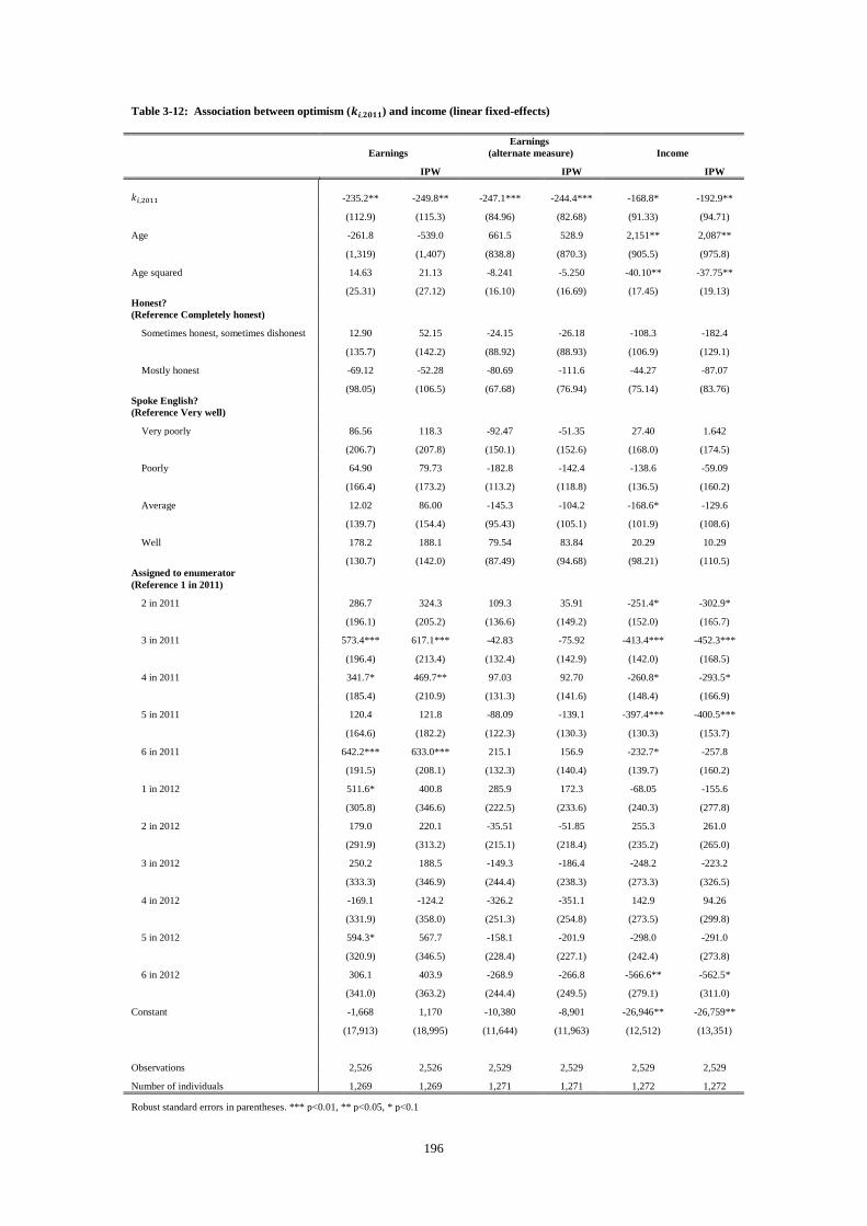
196

Table 3-12: Association between optimism (𝒌𝒊,𝟐𝟎𝟏𝟏) and income (linear fixed-effects)

Earnings

Earnings

(alternate measure) Income

IPW

IPW

IPW

𝑘𝑖,2011 -235.2** -249.8** -247.1*** -244.4*** -168.8* -192.9**

(112.9) (115.3) (84.96) (82.68) (91.33) (94.71)

Age -261.8 -539.0 661.5 528.9 2,151** 2,087**

(1,319) (1,407) (838.8) (870.3) (905.5) (975.8)

Age squared 14.63 21.13 -8.241 -5.250 -40.10** -37.75**

(25.31) (27.12) (16.10) (16.69) (17.45) (19.13)

Honest?

(Reference Completely honest)

Sometimes honest, sometimes dishonest 12.90 52.15 -24.15 -26.18 -108.3 -182.4

(135.7) (142.2) (88.92) (88.93) (106.9) (129.1)

Mostly honest -69.12 -52.28 -80.69 -111.6 -44.27 -87.07

(98.05) (106.5) (67.68) (76.94) (75.14) (83.76)

Spoke English?

(Reference Very well)

Very poorly 86.56 118.3 -92.47 -51.35 27.40 1.642

(206.7) (207.8) (150.1) (152.6) (168.0) (174.5)

Poorly 64.90 79.73 -182.8 -142.4 -138.6 -59.09

(166.4) (173.2) (113.2) (118.8) (136.5) (160.2)

Average 12.02 86.00 -145.3 -104.2 -168.6* -129.6

(139.7) (154.4) (95.43) (105.1) (101.9) (108.6)

Well 178.2 188.1 79.54 83.84 20.29 10.29

(130.7) (142.0) (87.49) (94.68) (98.21) (110.5)

Assigned to enumerator

(Reference 1 in 2011)

2 in 2011 286.7 324.3 109.3 35.91 -251.4* -302.9*

(196.1) (205.2) (136.6) (149.2) (152.0) (165.7)

3 in 2011 573.4*** 617.1*** -42.83 -75.92 -413.4*** -452.3***

(196.4) (213.4) (132.4) (142.9) (142.0) (168.5)

4 in 2011 341.7* 469.7** 97.03 92.70 -260.8* -293.5*

(185.4) (210.9) (131.3) (141.6) (148.4) (166.9)

5 in 2011 120.4 121.8 -88.09 -139.1 -397.4*** -400.5***

(164.6) (182.2) (122.3) (130.3) (130.3) (153.7)

6 in 2011 642.2*** 633.0*** 215.1 156.9 -232.7* -257.8

(191.5) (208.1) (132.3) (140.4) (139.7) (160.2)

1 in 2012 511.6* 400.8 285.9 172.3 -68.05 -155.6

(305.8) (346.6) (222.5) (233.6) (240.3) (277.8)

2 in 2012 179.0 220.1 -35.51 -51.85 255.3 261.0

(291.9) (313.2) (215.1) (218.4) (235.2) (265.0)

3 in 2012 250.2 188.5 -149.3 -186.4 -248.2 -223.2

(333.3) (346.9) (244.4) (238.3) (273.3) (326.5)

4 in 2012 -169.1 -124.2 -326.2 -351.1 142.9 94.26

(331.9) (358.0) (251.3) (254.8) (273.5) (299.8)

5 in 2012 594.3* 567.7 -158.1 -201.9 -298.0 -291.0

(320.9) (346.5) (228.4) (227.1) (242.4) (273.8)

6 in 2012 306.1 403.9 -268.9 -266.8 -566.6** -562.5*

(341.0) (363.2) (244.4) (249.5) (279.1) (311.0)

Constant -1,668 1,170 -10,380 -8,901 -26,946** -26,759**

(17,913) (18,995) (11,644) (11,963) (12,512) (13,351)

Observations 2,526 2,526 2,529 2,529 2,529 2,529

Number of individuals 1,269 1,269 1,271 1,271 1,272 1,272

Robust standard errors in parentheses. *** p<0.01, ** p<0.05, * p<0.1

197

Table 3-13: Association between optimism (𝒌𝒊,𝟐𝟎𝟏𝟏) and reservation wages (linear fixed-effects)

Log of reported

reservation wage

Log of reservation wage

if desperate

Difference between

reservation wage and earnings

IPW

IPW

IPW

𝑘𝑖,2011 0.0515* 0.0417 0.00564 0.0116 455.4*** 460.2***

(0.0276) (0.0287) (0.0293) (0.0311) (151.1) (162.1)

Age 0.265 0.199 0.137 0.114 1,960 2,114

(0.278) (0.304) (0.340) (0.369) (1,567) (1,757)

Age squared -0.00518 -0.00418 -0.00467 -0.00180 -40.43 -47.98

(0.00538) (0.00577) (0.00654) (0.00706) (30.11) (32.59)

Honest?

(Reference Completely honest)

Sometimes honest, sometimes

dishonest 0.0196 0.0245 0.0535 0.102* -85.24 -92.59

(0.0329) (0.0355) (0.0409) (0.0523) (179.2) (203.0)

Mostly honest 0.000907 0.00302 0.0132 0.00398 18.10 25.40

(0.0248) (0.0271) (0.0273) (0.0299) (134.7) (150.1)

Spoke English?

(reference Very well)

Very poorly -0.0190 0.00953 0.0120 -0.0301 -150.6 -192.7

(0.0619) (0.0624) (0.0823) (0.0916) (353.6) (374.3)

Poorly 0.0137 0.0379 -0.0986* -0.141** -77.31 -44.93

(0.0454) (0.0520) (0.0531) (0.0664) (241.7) (276.1)

Average -0.0151 0.0141 -0.0350 -0.0245 -116.9 -122.1

(0.0316) (0.0359) (0.0363) (0.0392) (177.4) (213.8)

Well 0.00863 0.0242 -0.0461 -0.0521 -203.3 -203.5

(0.0289) (0.0328) (0.0317) (0.0349) (172.2) (208.6)

Assigned to enumerator

(Reference 1 in 2011)

2 in 2011 -0.0701* -0.0483 -0.000191 -0.00307 -619.3** -471.9*

(0.0411) (0.0449) (0.0507) (0.0558) (241.8) (276.8)

3 in 2011 -0.131*** -0.111** 0.00350 0.0114 -968.0*** -872.0***

(0.0438) (0.0477) (0.0519) (0.0641) (243.4) (275.4)

4 in 2011 -0.0182 -0.00106 -0.0561 -0.0777 -372.2 -359.9

(0.0412) (0.0447) (0.0516) (0.0609) (248.2) (293.5)

5 in 2011 -0.134*** -0.123*** -0.0874* -0.0813 -567.3** -468.5

(0.0388) (0.0460) (0.0477) (0.0552) (225.8) (287.1)

6 in 2011 -0.462*** -0.409*** -0.188*** -0.169*** -2,066*** -1,782***

(0.0459) (0.0524) (0.0505) (0.0566) (257.2) (287.9)

1 in 2012 -0.100 -0.0721 0.000922 -0.0760 -1,124*** -741.0

(0.0748) (0.0857) (0.0873) (0.0977) (435.3) (527.3)

2 in 2012 -0.0616 -0.0280 0.0660 -0.0141 -617.5 -418.1

(0.0713) (0.0805) (0.0828) (0.0961) (403.5) (481.6)

3 in 2012 -0.0170 0.0240 0.0428 -0.0627 -577.7 -230.0

(0.0756) (0.0907) (0.0921) (0.117) (439.8) (528.3)

4 in 2012 -0.0647 -0.0186 -0.0440 -0.130 -351.9 -114.6

(0.0842) (0.0930) (0.0933) (0.105) (495.7) (565.2)

5 in 2012 -0.0423 -0.0117 -0.0527 -0.149 -841.5* -610.2

(0.0744) (0.0832) (0.0880) (0.101) (433.7) (502.3)

6 in 2012 0.0137 0.0717 0.183* 0.0974 -447.6 -152.2

(0.0768) (0.0827) (0.0959) (0.110) (447.5) (514.8)

Constant 4.907 5.901 6.915 5.785 -19,867 -19,242

(3.832) (4.257) (4.669) (5.125) (21,642) (25,005)

Observations 2,502 2,502 2,502 2,502 2,526 2,526

Number of i 1,269 1,269 1,272 1,272 1,269 1,269

Robust standard errors in parentheses. *** p<0.01, ** p<0.05, * p<0.1

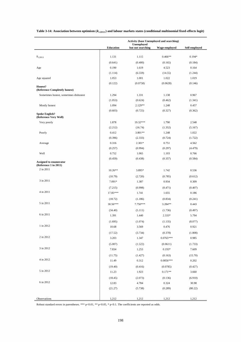
198

Table 3-14: Association between optimism (𝒌𝒊.𝟐𝟎𝟏𝟏) and labour markets states (conditional multinomial fixed-effects logit)

Activity (base Unemployed and searching)

Education

Unemployed

but not searching Wage-employed Self-employed

𝑘𝑖,2011

1.131 1.115 0.466** 0.194*

(0.641) (0.400) (0.165) (0.184)

Age 0.190 1.619 4.523 0.164

(1.114) (6.559) (14.55) (1.244)

Age squared 1.053 1.001 1.022 1.019

(0.122) (0.0758) (0.0628) (0.146)

Honest?

(Reference Completely honest)

Sometimes honest, sometimes dishonest 1.294 1.331 1.138 0.967

(1.053) (0.624) (0.462) (1.341)

Mostly honest 1.094 2.129** 1.248 0.457

(0.603) (0.725) (0.327) (0.362)

Spoke English?

(Reference Very Well)

Very poorly 1.878 19.32*** 1.790 2.548

(2.212) (16.74) (1.352) (5.167)

Poorly 0.412 3.801** 1.248 1.022

(0.396) (2.333) (0.724) (1.722)

Average 0.316 2.301* 0.751 4.562

(0.257) (0.994) (0.297) (4.479)

Well 0.752 1.065 1.103 0.766

(0.459) (0.438) (0.357) (0.584)

Assigned to enumerator

(Reference 1 in 2011)

2 in 2011 10.26** 3.895* 1.742 0.536

(10.79) (2.720) (0.785) (0.612)

3 in 2011 7.091* 1.387 0.934 0.309

(7.215) (0.998) (0.471) (0.407)

4 in 2011 17.85*** 1.741 1.655 0.186

(18.72) (1.186) (0.834) (0.241)

5 in 2011 30.56*** 7.750*** 3.284** 0.443

(34.40) (5.111) (1.736) (0.497)

6 in 2011 1.391 1.440 2.333* 5.794

(1.695) (1.074) (1.135) (8.077)

1 in 2012 10.68 3.569 0.476 0.921

(17.52) (3.734) (0.378) (1.808)

2 in 2012 3.203 1.347 0.0765*** 0.985

(5.007) (1.522) (0.0611) (1.733)

3 in 2012 7.834 1.253 0.193* 7.609

(11.75) (1.427) (0.163) (15.70)

4 in 2012 11.49 0.312 0.0856*** 0.202

(19.40) (0.416) (0.0785) (0.427)

5 in 2012 11.23 1.923 0.171** 3.660

(18.45) (2.073) (0.136) (6.910)

6 in 2012 12.83 4.784 0.324 30.98

(21.27) (5.738) (0.289) (80.22)

Observations 1,212 1,212 1,212 1,212

Robust standard errors in parentheses. *** p<0.01, ** p<0.05, * p<0.1. The coefficients are reported as odds.

199

Table 3-15: Association between optimism (𝒌𝒊.𝟐𝟎𝟏𝟏) and job satisfaction and, separately, wellbeing (conditional fixed-

effects multinomial logit)

Any job satisfaction

(base No job)

Wellbeing

(base OK)

Unhappy Not unhappy

Unhappy or very

unhappy

Happy or

very happy

𝑘𝑖,2011

0.766 0.565**

0.929 0.816

(0.269) (0.157)

(0.249) (0.234)

Age 174.9 17.79

0.672 0.113

(639.0) (50.07)

(1.970) (0.307)

Age squared 0.917 0.967

0.981 0.996

(0.0642) (0.0542)

(0.0535) (0.0532)

Honest?

(Reference Completely honest)

Sometimes honest, sometimes dishonest 0.545 0.873

1.317 2.133**

(0.267) (0.296)

(0.437) (0.729)

Mostly honest 0.719 0.607**

0.850 1.112

(0.244) (0.143)

(0.188) (0.254)

Spoke English?

(Reference Very Well)

Very poorly 1.397 1.088

1.168 0.596

(1.677) (0.657)

(0.839) (0.326)

Poorly 1.485 0.708

0.701 0.800

(0.877) (0.305)

(0.338) (0.366)

Average 1.834 0.920

1.070 0.816

(0.819) (0.293)

(0.343) (0.246)

Well 1.492 1.533

1.563* 1.151

(0.559) (0.413)

(0.422) (0.304)

Assigned to enumerator

(Reference 1 in 2011)

2 in 2011 0.567 1.115

0.325** 1.356

(0.322) (0.478)

(0.146) (0.588)

3 in 2011 0.893 1.622

0.259*** 1.601

(0.496) (0.708)

(0.119) (0.717)

4 in 2011 0.346* 0.875

0.258*** 1.051

(0.201) (0.366)

(0.124) (0.456)

5 in 2011 0.388* 0.408**

0.128*** 1.231

(0.207) (0.183)

(0.0562) (0.483)

6 in 2011 0.815 2.334*

0.298*** 0.668

(0.455) (1.064)

(0.124) (0.293)

1 in 2012 0.226 0.392

0.348 6.249***

(0.219) (0.280)

(0.255) (4.328)

2 in 2012 0.153* 0.115***

0.624 5.075**

(0.151) (0.0803)

(0.442) (3.334)

3 in 2012 0.203 0.177**

0.260* 4.679**

(0.202) (0.134)

(0.205) (3.346)

4 in 2012 0.0289*** 0.140**

0.246 14.78***

(0.0344) (0.115)

(0.215) (11.18)

5 in 2012 0.212 0.594

0.760 1.736

(0.202) (0.408)

(0.541) (1.238)

6 in 2012 0.107** 0.177**

0.652 7.936***

(0.109) (0.133)

(0.569) (6.053)

Observations 1,086 1,086

1,456 1,456

Robust standard errors in parentheses. *** p<0.01, ** p<0.05, * p<0.1. The coefficients are reported as odds.

200

Table 3-16: Estimated Average Treatment Effect of statement to respondents in KwaZulu-Natal (conditional fixed-effects

logit)

Job Any work Employed

Self-reported

employed

Searching

unemployed

Self-reported

unemployed Discouraged

Treatment 1.082 1.303 1.265 0.653 0.676 0.829 1.142

(0.508) (0.576) (0.709) (0.333) (0.281) (0.392) (0.592)

Assigned to

enumerator

(Reference 1

in 2011)

2 in 2011 0.857 1.010 1.517 0.690 0.697 1.240 4.047

(0.683) (0.861) (1.368) (0.527) (0.506) (1.025) (3.507)

3 in 2011 2.397 3.640 0.743 1.190 2.760 3.818 5.382**

(2.242) (3.433) (0.737) (1.267) (2.029) (3.348) (4.442)

4 in 2011 1.128 0.964 0.710 1.686 0.924 1.875 2.945

(0.881) (0.744) (0.611) (1.411) (0.627) (1.437) (2.390)

5 in 2011 0.771 0.993 1.170 0.409 0.537 1.178 4.203**

(0.587) (0.780) (1.020) (0.293) (0.314) (0.820) (2.872)

6 in 2011 0.898 1.133 0.632 0.999 1.598 3.780* 4.775**

(0.796) (1.013) (0.765) (0.915) (1.171) (3.007) (3.800)

1 in 2012 1.015 1.305 2.520 2.246 0.636 0.910 1.836

(0.913) (1.174) (2.768) (2.255) (0.454) (0.748) (1.855)

2 in 2012 0.0831** 0.0825** 0.312 0.194** 1.124 1.124 3.513*

(0.0816) (0.0818) (0.288) (0.147) (0.710) (0.879) (2.559)

3 in 2012 0.245 0.235 0.503 0.426 0.427 0.940 1.685

(0.227) (0.224) (0.433) (0.377) (0.256) (0.587) (1.103)

4 in 2012 0.616 0.711 1.003 0.566 0.817 0.441 4.103

(0.524) (0.585) (0.957) (0.491) (0.557) (0.392) (3.816)

5 in 2012 0.748 1.178 0.556 0.517 0.758 1.678 5.031**

(0.546) (0.935) (0.466) (0.352) (0.535) (1.285) (3.402)

6 in 2012 0.674 0.718 3.957 1.249 0.329* 0.0901** 0.668

(0.535) (0.558) (3.391) (0.991) (0.216) (0.0895) (0.631)

Observations 210 234 132 174 256 220 190

Robust standard errors in parentheses. *** p<0.01, ** p<0.05, * p<0.1. The coefficients are reported as odds.

201

Table 3-17: Estimated Average Treatment Effect of statement to respondents in KwaZulu-Natal (linear fixed-effects

estimator)

Earnings

Earnings

(alternate

measure) Income

Log reservation

wage

Log reservation

wage

if desperate

Difference

between

reservation

wage and

earnings

Treatment 259.4 -34.68 -104.3 -0.00131 -0.0448 -143.8

(192.3) (152.0) (172.4) (0.0507) (0.0683) (276.2)

Assigned to

enumerator

(Reference 1 in

2011)

2 in 2011 -411.7 -128.5 -367.4 -0.175** -0.0745 -267.2

(301.5) (250.7) (362.0) (0.0856) (0.120) (444.8)

3 in 2011 241.1 -30.80 -755.2*** -0.290*** 0.0937 -1,858***

(291.5) (215.1) (260.5) (0.0826) (0.119) (431.5)

4 in 2011 185.3 302.8 -470.5* -0.141 -0.262** -619.9

(296.9) (268.5) (277.2) (0.0914) (0.118) (513.9)

5 in 2011 -217.7 -214.5 -529.2* -0.331*** -0.193* -1,016**

(295.0) (239.4) (275.3) (0.0796) (0.102) (415.6)

6 in 2011 -511.2 -111.1 -344.8 -0.215** -0.178 -282.9

(347.1) (251.6) (320.5) (0.0925) (0.119) (519.0)

1 in 2012 -56.88 116.6 -466.7 -0.245*** -0.0605 -1,193***

(313.3) (246.3) (288.6) (0.0830) (0.106) (459.3)

2 in 2012 -1,091*** -840.3*** -62.24 -0.162* -0.0284 67.60

(317.0) (259.9) (296.5) (0.0822) (0.106) (450.0)

3 in 2012 -239.0 -556.3*** -539.9* -0.214** -0.120 -693.1

(242.6) (202.1) (287.9) (0.0867) (0.118) (424.6)

4 in 2012 -840.4** -591.6* -24.69 -0.198** -0.0478 -312.9

(374.5) (353.9) (425.2) (0.0998) (0.114) (622.3)

5 in 2012 148.8 -134.7 -301.1 -0.0884 -0.0272 -623.1

(303.9) (215.0) (261.6) (0.0884) (0.121) (424.4)

6 in 2012 -250.9 -354.1 -523.1** 0.0793 0.165 102.0

(295.1) (244.4) (264.8) (0.0868) (0.120) (492.7)

Constant 1,122*** 822.5*** 1,577*** 8.430*** 7.475*** 3,979***

(170.6) (147.2) (201.3) (0.0556) (0.0730) (292.2)

Observations 670 664 534 522 550 542

Number of i 335 332 267 261 275 271

Robust standard errors in parentheses. *** p<0.01, ** p<0.05, * p<0.1

202

Discussion and conclusion

The descriptions and estimates that we have presented in this chapter suggest that a high

proportion of young South Africans may be optimistic about their employment prospects.

These young workers not only report reservation wages that are significantly higher than what

these young people in our sample are earning (or go on to earn) but they also believe their

chances of receiving wage offers that are larger than their reported reservation wages are

higher than the data in our sample suggests they are. This optimism persists even when these

young people are given reliable information about the labour market prospects of their peers.

There is a robust positive correlation between optimism in 2011 and subsequent

unemployment in 2012. The inferences we are able to draw from these estimates are however

limited. First it is unclear that our sample is representative of South African youth more

generally. Secondly those young workers that are optimistic may be less likely to remain

employed regardless of their expectations. The results we present in this chapter merely

demonstrate that some of this optimism may be misguided, although the respondents in our

sample that are optimistic may have fared even worse had they not been optimistic. It does

not appear though that these transitions from employment into unemployment are associated

with a decrease in wellbeing. Rather we find that relatively optimistic individuals are less

likely to be employed in jobs where they are not unhappy with the job.

It is nevertheless telling that the workers in our sample that are optimistic are less likely to

stay employed and that giving these individuals reliable information about their labour market

prospects in South Africa has no effect on their labour market outcomes and reported

reservation wages. This has important implications for policy in South Africa because it

suggests that many young South Africans will ultimately be disappointed. The evidence we

present in this chapter also suggests that young South Africans may report reservations wages

that are higher than what they can expect to earn not only because they have limited

203

information but also because they may not have the skills required to assess their value to

firms in South Africa.

204

References

1. Banerjee, A., Galiani, S., Levinsohn, J., McLaren, Z., and Woolard, I. (2008).

Why has unemployment risen in the new South Africa? Economics of Transition,

16(4), 715-740.

2. Beaulier, S. and Caplan, B. (2007), Behavioral Economics and Perverse Effects

of the Welfare State. Kyklos, 60: 485–507

3. Chamberlain, G. 1980. Analysis of covariance with qualitative data. Review of

Economic Studies 47: 225–238.

4. Dewing, S., Mathews, C., Fatti, G., Grimwood, A., and Boulle, A. (2014).

Antiretroviral Adherence Interventions in Southern Africa: Implications for

Using HIV Treatments for Prevention. Current HIV/AIDS Reports, 11(1), 63-71.

5. Diagne, A., and Irene, M. F. (2009). Essays on the economics of information,

education and job search. University of California, Berkeley.

6. Dohmen, T. J. (2014). Behavioural Labour Economics: Advances and Future

Directions. Labour Economics. Volume 30.

7. Dunning, D., Johnson, K., Ehrlinger, J., and Kruger, J. (2003). Why people fail to

recognize their own incompetence. Current Directions in Psychological Science,

12, pp. 83–86

8. Eckstein, Z. and van den Berg, G. J. (2007). Empirical labor search: A survey.

Journal of Econometrics 136(2), 531-564.

9. Ehrlinger, J., Johnson, D., Banner, M., Dunning, D., and Kruger, J. (2008). Why

the unskilled are unaware? Further explorations of (lack of) self-insight among

the incompetent. Organizational Behavior and Human Decision Processes, 105,

pp. 98–121

10. Falk, A., Huffman, D. and Sunde, U. (2006 a). Self-Confidence and Search. IZA

DP No. 2525. Institute for the Study of Labor.

205

11. Falk, A., Huffman, D. and Sunde, U. (2006 b). Do I have what it takes?

Equilibrium search with type uncertainty and non-participation. Institute for the

Study of Labor

12. Ferraro, P. (2010). Know thyself: Competence and self-awareness. Atlantic

Economic Journal, 38, pp. 183–196.

13. Groh, M., McKenzie, D., Shammout, N., and Vishwanath, T. (2014). Testing the

importance of search frictions, matching, and reservation prestige through

randomized experiments in Jordan. World Bank Policy Research Working Paper,

(7030).

14. Haun, D., and Zeringue, A., Leach, A., and Foley, A. (2000). Assessing the

competence of specimen-processing personnel. Laboratory Medicine, 31, pp.

633–637

15. Heine, S. J., and Lehman, D. (1995). Cultural variation in unrealistic optimism:

Does the West feel more vulnerable than the East? Journal of Personality and

Social Psychology, Vol 68(4), Apr 1995, 595-607

16. Krueger, J., and Mueller, R. A. (2002). Unskilled, unaware, or both? The

contribution of social–perceptual skills and statistical regression to self-

enhancement biases. Journal of Personality and Social Psychology, 82 (2002), pp.

180–188

17. Johnson, D. D. P., and Fowler, J. H. (2011). The evolution of overconfidence.

Nature 477, 317–320

18. Burson, K. A., Larrick, R. P., and Klayman, J. (2006). Skilled or unskilled, but

still unaware of it: How perceptions of difficulty drive miscalibration in relative

comparisons.

19. Kahneman, D. 2003. Maps of bounded rationality: psychology for behavioral

economics. The American Economic Review 93 (5): 1449–75

206

20. Kingdon, G. and Knight, J. (2001). Unemployment in South Africa: The Nature

of the Beast. WPS/2001-15, Centre for the Study of African Economies,

Department of Economics, University of Oxford

21. Krajč, M. and Ortmann, A. (2008). Are the unskilled really that unaware? An

alternative explanation. Journal of Economic Psychology, 29 (2008), pp. 724–738

22. Kruger, J. and Dunning, D. (1999). Unskilled and Unaware of It: How

Difficulties in Recognizing One's Own Incompetence Lead to Inflated Self-

Assessments. Journal of Personality and Social Psychology 77 (6): 1121–3

23. Babcock, L., Congdon, W., Katz, L. and Mullainathan, S. (2012). Notes on

behavioral economics and labor market policy. IZA Journal of Labor Policy,

Springer, vol. 1(1), pages 1-14, December.

24. Ackerman, P.L., Beier, M.B. and Bowen, K.R. (2002). What we really know

about our abilities and our knowledge. Personality and Individual Differences, 34

(2002), pp. 587–605.

25. Park, Y., and Santos-Pinto, L. (1010). Overconfidence in tournaments: Evidence

from the field. Theory and Decision, 69, pp. 143–166

26. Posel, D. (2014). Self-assessed well-being and economic rank in South Africa.

Development Southern Africa, 31(1), 51-64.

27. Posel, D. R. and Casale, D. M. (2011). Relative standing and subjective well-

being in South Africa: The role of perceptions, expectations and income mobility.

Social Indicators Research, 104(2), 195-223.

28. Pforr, K. (2014). femlogit-Implementation of the multinomial logit model with

fixed effects. Stata Journal, 14(4), 847-862.

29. Rabin, M. (1998). Psychology and Economics. Journal of Economic Literature.

36: 11–46.

30. Rabin, M. (2013). Incorporating limited rationality into economics. Journal of

Economic Literature, 51(2), 528-543.

207

31. Rogerson, R., Shimer, R., and Wright, R. (2004). Search-theoretic models of the

labor market-a survey. (No. w10655). National Bureau of Economic Research.

32. Santos-Pinto, L. and Sobel, J. (2005). “A model of positive self-image in

subjective assessments.” American Economic Review, 1386-1402, American

Economic Association.

33. Schlösser, T., Dunning, D., Johnson, K. L. and Kruger, J. (2013). How unaware

are the unskilled? Empirical tests of the “signal extraction” counterexplanation

for the Dunning–Kruger effect in self-evaluation of performance. Journal of

Economic Psychology, 39, 85-100.

34. Spinnewijn, J. (forthcoming). Optimal insurance design with biased beliefs. J.

Eur. Econ. Association.

35. Van den Steen, E. (2004). Rational overoptimism (and other biases). American

Economic Review, 4: 1141– 1151, American Economic Association.

208

Appendix

Table A3-1: Assignment to and allocation of surveys among enumerators in 2011 and 2012 (Number of observations)

Assigned to enumerator (in 2011)

One Two Three Four Five Six Total

Number interviewed in

2011

Gauteng 215 192 185 191 199 194 1,176

KwaZulu-Natal 74 63 64 65 65 63 394

Limpopo 134 127 132 129 130 136 788

Total 423 382 381 385 394 393 2,358

Proportion of that were

interviewed in 2012 (%)

Gauteng 74 76 74 67 75 75 74

KwaZulu-Natal 59 68 69 66 88 71 70

Limpopo 83 77 79 79 78 77 79

Total 74 75 75 71 78 75 75

Number interviewed by

enumerator in 2011

Enumerator: 1 382 17 4 6 3 18 430

Enumerator: 2 8 201 17 19 9 25 279

Enumerator: 3 0 1 267 0 0 0 268

Enumerator: 4 2 2 2 326 3 15 350

Enumerator: 5 6 7 8 2 367 14 404

Enumerator: 6 0 0 0 0 0 288 288

Enumerator: 7 12 144 17 32 6 23 234

Enumerator: 8 13 10 66 0 6 10 105

Assigned to enumerator (in 2012)

One Two Three Four Five Six Total

Number assigned in 2012

Gauteng 240 253 214 127 179 162 1,175

KwaZulu-Natal 70 91 67 39 62 65 394

Limpopo 176 178 133 86 119 96 788

Total 486 522 414 252 360 323 2,357

Proportion that were

interviewed in 2012 (%)

Gauteng 75 69 72 76 82 71 74

KwaZulu-Natal 66 63 78 74 84 62 70

Limpopo 84 76 83 77 77 73 79

Total 77 70 77 76 81 70 75

Number interviewed by

enumerator in 2012

Enumerator: 9 368 11 0 1 2 9 391

Enumerator: 10 5 0 7 7 4 10 33

Enumerator: 11 5 352 28 26 23 14 448

Enumerator: 12 2 27 311 8 15 9 372

Enumerator: 13 0 0 1 161 8 0 170

Enumerator: 14 0 2 0 0 246 0 248

Enumerator: 15 3 2 0 0 0 198 203

209

Table A3-2: Comparison of the characteristics of the respondents in 2011 that are excluded from and in the balanced

panel (Number of observations and percentage of respondents)

Excluded Panel

Excluded Panel

Gender

School education

Male 488 539

Grade 12 784 920

% 44.94 42.37

% 72.19 72.33

Female 598 733

Grade 11 204 247

% 55.06 57.63

% 18.78 19.42

Less than Grade 11 86 95

Age

% 7.92 7.47

Other 12 10

19 1 0

% 1.1 0.79

% 0.09 0

20 4 0

Tertiary education

% 0.37 0

21 38 0

Only school 622 692

% 3.5 0

% 57.27 54.4

22 145 162

Certificate 327 452

% 13.35 12.74

% 30.11 35.53

23 237 260

Diploma 108 105

% 21.82 20.44

% 9.94 8.25

24 220 265

Degree 29 23

% 20.26 20.83

% 2.67 1.81

25 206 273

% 18.97 21.46

Primary activity

26 170 238

% 15.65 18.71

School 23 14

27 59 74

% 2.12 1.1

% 5.43 5.82

Tertiary education 161 52

28 4 0

% 14.83 4.09

% 0.37 0

Unemployed and not searching for work 128 189

29 2 0

% 11.79 14.86

0.18 0

Unemployed and searching for work 331 581

% 30.48 45.68

Working for someone else 410 389

% 37.75 30.58

Self employed 33 47

% 3.04 3.69

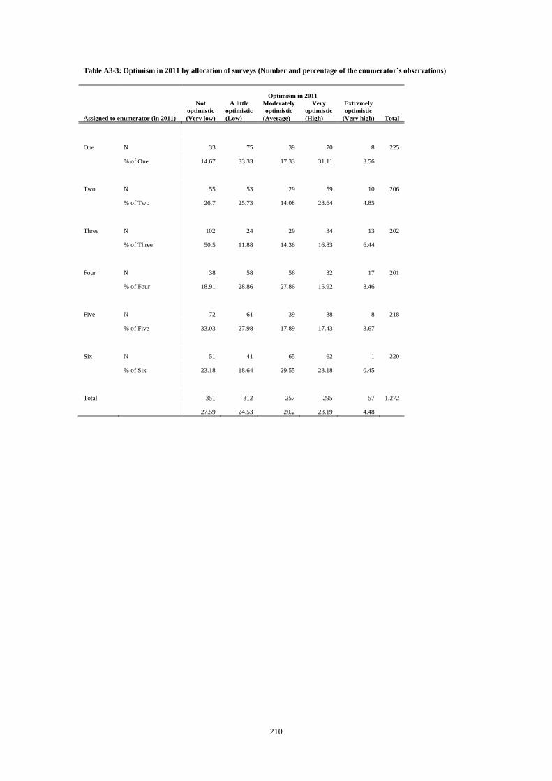
210

Table A3-3: Optimism in 2011 by allocation of surveys (Number and percentage of the enumerator’s observations)

Optimism in 2011

Assigned to enumerator (in 2011)

Not

optimistic

(Very low)

A little

optimistic

(Low)

Moderately

optimistic

(Average)

Very

optimistic

(High)

Extremely

optimistic

(Very high) Total

One N 33 75 39 70 8 225

% of One 14.67 33.33 17.33 31.11 3.56

Two N 55 53 29 59 10 206

% of Two 26.7 25.73 14.08 28.64 4.85

Three N 102 24 29 34 13 202

% of Three 50.5 11.88 14.36 16.83 6.44

Four N 38 58 56 32 17 201

% of Four 18.91 28.86 27.86 15.92 8.46

Five N 72 61 39 38 8 218

% of Five 33.03 27.98 17.89 17.43 3.67

Six N 51 41 65 62 1 220

% of Six 23.18 18.64 29.55 28.18 0.45

Total

351 312 257 295 57 1,272

27.59 24.53 20.2 23.19 4.48

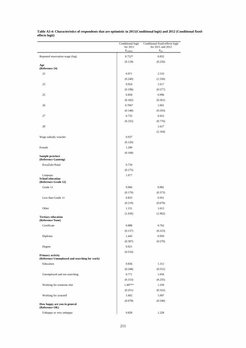
211

Table A3-4: Characteristics of respondents that are optimistic in 2011(Conditional logit) and 2012 (Conditional fixed-

effects logit)

Conditional logit

for 2011

𝑘𝑖,2011

Conditional fixed-effects logit

for 2011 and 2012

𝑘𝑖,t

Reported reservation wage (log) 0.752* 0.832

(0.118) (0.226)

Age

(Reference 24)

22 0.971 2.533

(0.240) (1.536)

23 0.924 1.617

(0.198) (0.577)

25 0.858 0.996

(0.182) (0.361)

26 0.706* 1.001

(0.148) (0.593)

27 0.735 0.922

(0.235) (0.776)

28

1.617

(2.164)

Wage subsidy voucher 0.937

(0.126)

Female 1.200

(0.168)

Sample province

(Reference Gauteng)

KwaZulu-Natal 0.734

(0.175)

Limpopo 1.077

School education

(Reference Grade 12)

Grade 11 0.966 0.881

(0.170) (0.373)

Less than Grade 11 0.833 0.951

(0.219) (0.670)

Other 1.151 1.613

(1.030) (1.902)

Tertiary education

(Reference None)

Certificate 0.888 0.762

(0.137) (0.223)

Diploma 1.443 0.950

(0.397) (0.570)

Degree 0.921

(0.516)

Primary activity

(Reference Unemployed and searching for work)

Education 0.836 1.312

(0.248) (0.551)

Unemployed and not searching 0.771 1.056

(0.153) (0.255)

Working for someone else 1.497** 1.259

(0.251) (0.322)

Working for yourself 1.602 1.097

(0.678) (0.546)

How happy are you in general

(Reference OK)

Unhappy or very unhappy 0.828 1.228

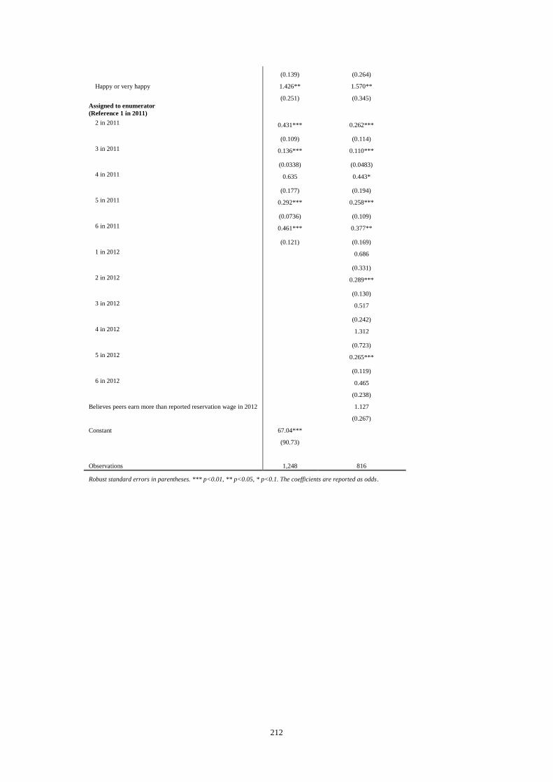
212

(0.139) (0.264)

Happy or very happy 1.426** 1.570**

(0.251) (0.345)

Assigned to enumerator

(Reference 1 in 2011)

2 in 2011 0.431*** 0.262***

(0.109) (0.114)

3 in 2011 0.136*** 0.110***

(0.0338) (0.0483)

4 in 2011 0.635 0.443*

(0.177) (0.194)

5 in 2011 0.292*** 0.258***

(0.0736) (0.109)

6 in 2011 0.461*** 0.377**

(0.121) (0.169)

1 in 2012

0.686

(0.331)

2 in 2012

0.289***

(0.130)

3 in 2012

0.517

(0.242)

4 in 2012

1.312

(0.723)

5 in 2012

0.265***

(0.119)

6 in 2012

0.465

(0.238)

Believes peers earn more than reported reservation wage in 2012

1.127

(0.267)

Constant 67.04***

(90.73)

Observations 1,248 816

Robust standard errors in parentheses. *** p<0.01, ** p<0.05, * p<0.1. The coefficients are reported as odds.

213

This page is intentionally left blank.

214

Conclusion

The chapters in this thesis present three separate studies on the dimensions of youth

unemployment in South Africa. In the first we ask “Is there first order short term state

dependence in unemployment among young South Africans?” State dependence in

unemployment is the effect of unemployment on future unemployment. This effect may arise

for many reasons although transaction costs are often regarded as a prominent cause of state

dependence in unemployment. Regardless of the underlying reason for state dependence in

unemployment, short-run policies to facilitate the employment of unemployed youth will only

reduce equilibrium unemployment if there is state dependence in unemployment. Thus we

would expect short term employment interventions to have a larger effect when they are

targeted at ages where there are higher levels of state dependence in unemployment. This

would provide a justification for targeting workers by their age. Our analysis reveals that

there is significant state dependence in unemployment from both short term and long term

unemployment among African South African males and females aged 19 to 39. When we

examine the relationship between age and state dependence in unemployment among young

South Africans though we find that the first order short term effects of unemployment on

future unemployment are not necessarily higher among those aged 20 to 24 than they are for

those aged 25 to 29. Further we find that there are significant levels of state dependence in

unemployment even among workers that are older (35-39) than the expanded definition of

youth in South Africa.

In the second chapter we ask “Does a targeted wage subsidy voucher have an effect on the

reservation wages of young South Africans?” We find, using an experiment, that a wage

subsidy voucher has no effect on the reservation wages of young South Africans one year

after it was allocated even though it led to an increase in employment among the

beneficiaries. However we also find that the measures of the reservation wage used in much

of the literature in South Africa are likely to suffer from non-classical measurement error. The

215

beneficiaries in our experiment were more likely than those in the control group to be

working in jobs where the reported wage is less than the worker’s reported reservation wage

and in jobs where the worker is unhappy with the job. They were also more likely to tell us

that the pay in these jobs is too low or they do not like the job or work environment when we

asked them why they are unhappy (or happy) with the job. We conclude that policy-makers

may find it difficult to raise both the level of employment and perceived wellbeing among

young South Africans through interventions without some pressure on the fiscus.

In the third chapter we ask “Are young South Africans overly optimistic about their labour

market prospects?” We find that many young South Africans may be optimistic about the

wage-offers they believe they will receive even though unemployment is pervasive among

youth in South Africa. A large proportion of the young South Africans in our sample remain

optimistic when they are given reliable information about the employment prospects of their

peers and there is a negative association between being optimistic and subsequent

employment. Furthermore we show, using an experiment, that giving a group of South

African youth this information about the labour market prospects of their peers has no effect

on their labour market outcomes and reported reservation wages one year later. Our research

is to the best of our knowledge the first to frame the behaviour of young workers in South

Africa as a departure from the assumption that these workers will revise their expectations

about wage offers when they are given reliable information about the labour market prospects

of young South Africans. The inferences we draw from this analysis are however limited.

Those young employed workers that are optimistic about their employment prospects may be

less likely to remain employed regardless of their expectations. Nevertheless we believe that

these findings have important implications for policy in South Africa because they imply that

many young South Africans will be disappointed. Furthermore South African youth that do

not revise their reported reservations downward when they are confronted with

unemployment may not only have limited information about what they can reasonably expect

216

to earn but they may also not have the skills required to form more realistic assessments of

their labour market prospects when they receive more reliable information.

The essays in this thesis are by no means an exhaustive account of the dimensions of youth

unemployment in South Africa. A key finding from our review of the literature is that we

need more evidence on the efficacy of the numerous interventions that have been proposed or

are being implemented. There is considerable scope for further research of existing

programmes or new ideas. However as we have noted throughout this thesis evaluating the

relationship between age, unemployment, and the effects of any employment interventions is

a demanding undertaking both in terms of the data that we require and the limits of what we

can demonstrate with any data. It is also unlikely that the evidence we generate when we pilot

interventions will correspond to the effects of these interventions at the scale required to

reverse the rising levels of unemployment among both younger and older workers in South

Africa. Furthermore it is unclear if the past is a reasonable reflection of future levels of

aggregate demand in this country.

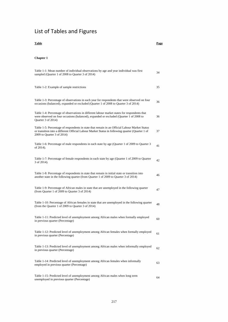
217

List of Tables and Figures

Table Page

Chapter 1

Table 1-1: Mean number of individual observations by age and year individual was first

sampled (Quarter 1 of 2008 to Quarter 3 of 2014) 34

Table 1-2: Example of sample restrictions 35

Table 1-3: Percentage of observations in each year for respondents that were observed on four

occasions (balanced), expanded or excluded (Quarter 1 of 2008 to Quarter 3 of 2014) 36

Table 1-4: Percentage of observations in different labour market states for respondents that

were observed on four occasions (balanced), expanded or excluded (Quarter 1 of 2008 to

Quarter 3 of 2014)

36

Table 1-5: Percentage of respondents in state that remain in an Official Labour Market Status

or transition into a different Official Labour Market Status in following quarter (Quarter 1 of 2009 to Quarter 3 of 2014)

37

Table 1-6: Percentage of male respondents in each state by age (Quarter 1 of 2009 to Quarter 3

of 2014). 41

Table 1-7: Percentage of female respondents in each state by age (Quarter 1 of 2009 to Quarter

3 of 2014). 42

Table 1-8: Percentage of respondents in state that remain in initial state or transition into another state in the following quarter (from Quarter 1 of 2009 to Quarter 3 of 2014)

46

Table 1-9: Percentage of African males in state that are unemployed in the following quarter

(from Quarter 1 of 2009 to Quarter 3 of 2014) 47

Table 1-10: Percentage of African females in state that are unemployed in the following quarter

(from the Quarter 1 of 2009 to Quarter 3 of 2014) 48

Table 1-11: Predicted level of unemployment among African males when formally employed

in previous quarter (Percentage) 60

Table 1-12: Predicted level of unemployment among African females when formally employed in previous quarter (Percentage)

61

Table 1-13: Predicted level of unemployment among African males when informally employed

in previous quarter (Percentage) 62

Table 1-14: Predicted level of unemployment among African females when informally

employed in previous quarter (Percentage) 63

Table 1-15: Predicted level of unemployment among African males when long term

unemployed in previous quarter (Percentage) 64

218

Table 1-16: Predicted level of unemployment among African females when long term unemployed in previous quarter (Percentage)

65

Table 1-17: Predicted level of unemployment among African males when short term

unemployed in previous quarter (Percentage) 66

Table 1-18: Predicted level of unemployment among African females when short term

unemployed in previous quarter (Percentage) 67

Table 1-19: Predicted level of unemployment from formal employment less predicted level of

unemployment from long term unemployment (among African males, percentage) 70

Table 1-20: Predicted level of unemployment from formal employment less predicted level of unemployment from long term unemployment (among African females, percentage)

71

Table 1-21: Predicted level unemployment from informal employment less predicted level of

unemployment from long term unemployment (among African males, percentage) 72

Table 1-22: Predicted level of unemployment from informal employment less predicted level of

unemployment from long term unemployment (among African females, percentage) 73

Table 1-23: Predicted level of unemployment from formal employment less predicted level of

unemployment from short term unemployment (among African males, percentage) 74

Table 1-24: Predicted level of unemployment from formal employment less predicted level of unemployment from short term unemployment (among African females, percentage)

75

Table 1-25: Predicted level of unemployment from informal employment less predicted level of

unemployment from short term unemployment (among African males, percentage) 76

Table 1-26: Predicted level of unemployment from informal employment less predicted level of

unemployment from short term unemployment (among African females, percentage) 77

Table 1-27: Predicted level of unemployment from long term unemployment less predicted

level of unemployment from short term unemployment (among African males, percentage) 78

Table 1-28: Predicted level of unemployment from long term unemployment less predicted level of unemployment from short term unemployment (among African females, percentage)

79

Table A1-1: Number of observations by year 85

Table A1-2: Estimates for African males age 19 to 24 in 2013/14 (Random-effects Probit) 86

Table A1-3: Estimates for African males age 25 to 29 in 2013/14 (Random-effects Probit) 87

Table A1-4: Estimates for African males age 30 to 34 in 2013/14 (Random-effects Probit) 88

Table A1-5: Estimates for African males age 35 to 39 in 2013/14 (Random-effects Probit) 89

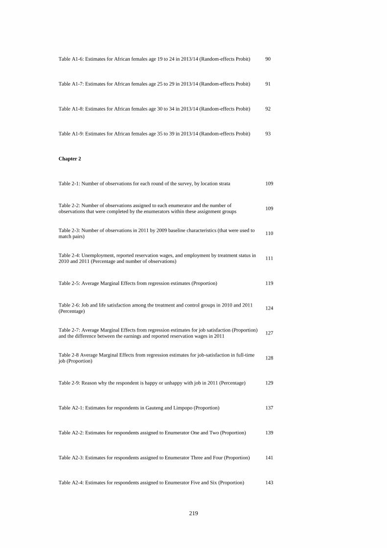
219

Table A1-6: Estimates for African females age 19 to 24 in 2013/14 (Random-effects Probit) 90

Table A1-7: Estimates for African females age 25 to 29 in 2013/14 (Random-effects Probit) 91

Table A1-8: Estimates for African females age 30 to 34 in 2013/14 (Random-effects Probit) 92

Table A1-9: Estimates for African females age 35 to 39 in 2013/14 (Random-effects Probit) 93

Chapter 2

Table 2-1: Number of observations for each round of the survey, by location strata 109

Table 2-2: Number of observations assigned to each enumerator and the number of

observations that were completed by the enumerators within these assignment groups 109

Table 2-3: Number of observations in 2011 by 2009 baseline characteristics (that were used to

match pairs) 110

Table 2-4: Unemployment, reported reservation wages, and employment by treatment status in 2010 and 2011 (Percentage and number of observations)

111

Table 2-5: Average Marginal Effects from regression estimates (Proportion) 119

Table 2-6: Job and life satisfaction among the treatment and control groups in 2010 and 2011

(Percentage) 124

Table 2-7: Average Marginal Effects from regression estimates for job satisfaction (Proportion)

and the difference between the earnings and reported reservation wages in 2011 127

Table 2-8 Average Marginal Effects from regression estimates for job-satisfaction in full-time job (Proportion)

128

Table 2-9: Reason why the respondent is happy or unhappy with job in 2011 (Percentage) 129

Table A2-1: Estimates for respondents in Gauteng and Limpopo (Proportion) 137

Table A2-2: Estimates for respondents assigned to Enumerator One and Two (Proportion) 139

Table A2-3: Estimates for respondents assigned to Enumerator Three and Four (Proportion) 141

Table A2-4: Estimates for respondents assigned to Enumerator Five and Six (Proportion) 143

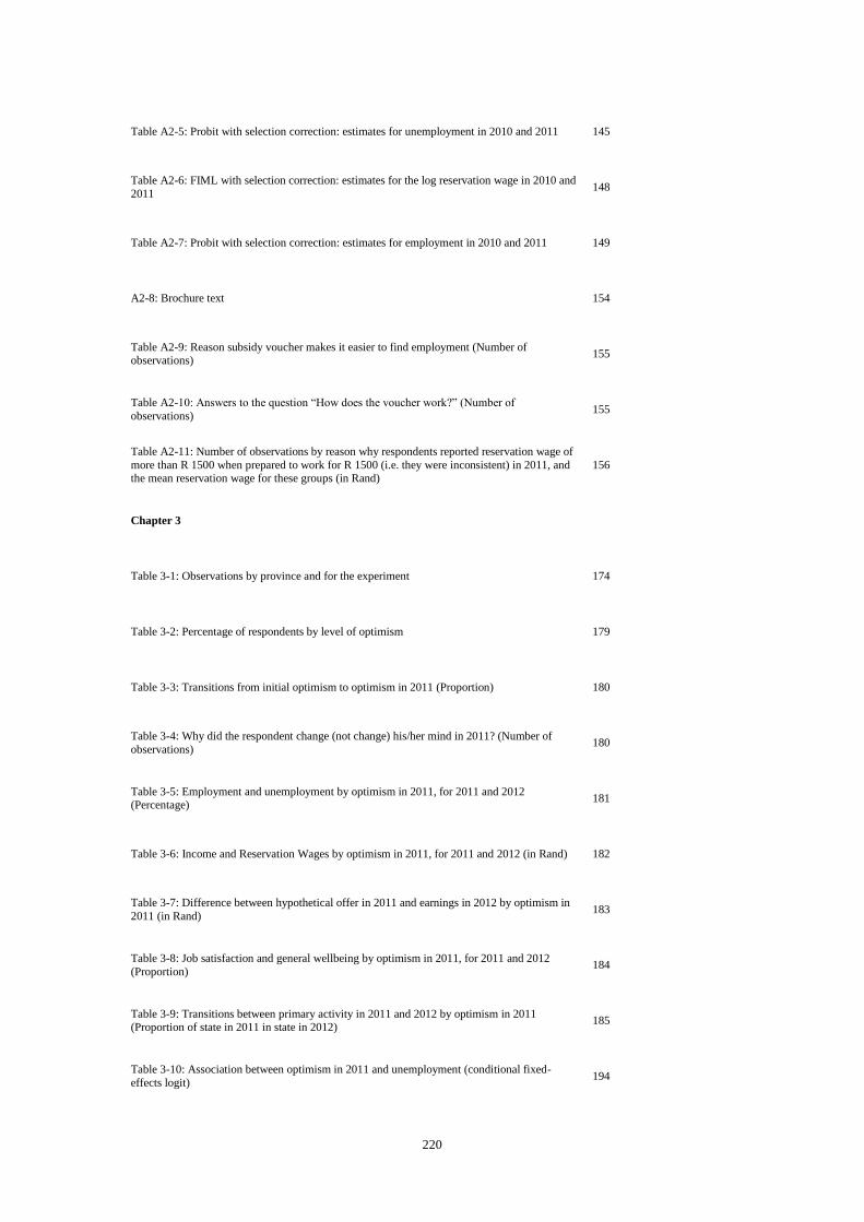
220

Table A2-5: Probit with selection correction: estimates for unemployment in 2010 and 2011 145

Table A2-6: FIML with selection correction: estimates for the log reservation wage in 2010 and

2011 148

Table A2-7: Probit with selection correction: estimates for employment in 2010 and 2011 149

A2-8: Brochure text 154

Table A2-9: Reason subsidy voucher makes it easier to find employment (Number of observations)

155

Table A2-10: Answers to the question “How does the voucher work?” (Number of

observations) 155

Table A2-11: Number of observations by reason why respondents reported reservation wage of

more than R 1500 when prepared to work for R 1500 (i.e. they were inconsistent) in 2011, and the mean reservation wage for these groups (in Rand)

156

Chapter 3

Table 3-1: Observations by province and for the experiment 174

Table 3-2: Percentage of respondents by level of optimism 179

Table 3-3: Transitions from initial optimism to optimism in 2011 (Proportion) 180

Table 3-4: Why did the respondent change (not change) his/her mind in 2011? (Number of

observations) 180

Table 3-5: Employment and unemployment by optimism in 2011, for 2011 and 2012 (Percentage)

181

Table 3-6: Income and Reservation Wages by optimism in 2011, for 2011 and 2012 (in Rand) 182

Table 3-7: Difference between hypothetical offer in 2011 and earnings in 2012 by optimism in

2011 (in Rand) 183

Table 3-8: Job satisfaction and general wellbeing by optimism in 2011, for 2011 and 2012

(Proportion) 184

Table 3-9: Transitions between primary activity in 2011 and 2012 by optimism in 2011 (Proportion of state in 2011 in state in 2012)

185

Table 3-10: Association between optimism in 2011 and unemployment (conditional fixed-

effects logit) 194

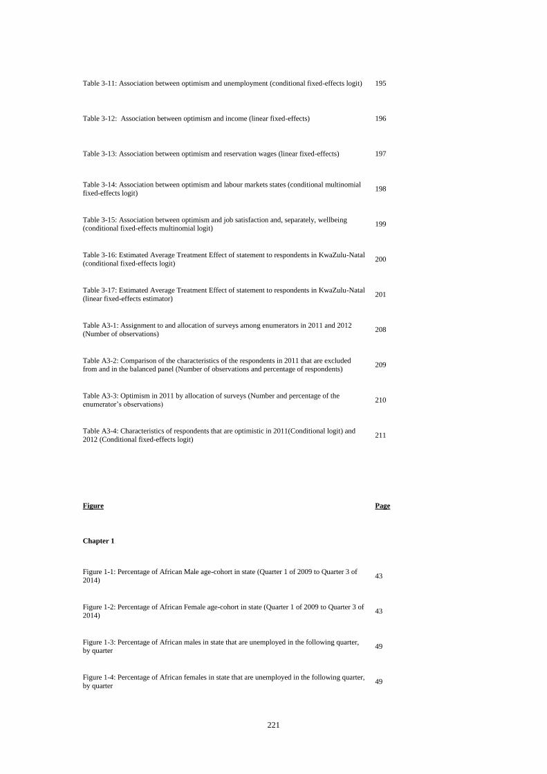
221

Table 3-11: Association between optimism and unemployment (conditional fixed-effects logit) 195

Table 3-12: Association between optimism and income (linear fixed-effects) 196

Table 3-13: Association between optimism and reservation wages (linear fixed-effects) 197

Table 3-14: Association between optimism and labour markets states (conditional multinomial

fixed-effects logit) 198

Table 3-15: Association between optimism and job satisfaction and, separately, wellbeing (conditional fixed-effects multinomial logit)

199

Table 3-16: Estimated Average Treatment Effect of statement to respondents in KwaZulu-Natal

(conditional fixed-effects logit) 200

Table 3-17: Estimated Average Treatment Effect of statement to respondents in KwaZulu-Natal

(linear fixed-effects estimator) 201

Table A3-1: Assignment to and allocation of surveys among enumerators in 2011 and 2012

(Number of observations) 208

Table A3-2: Comparison of the characteristics of the respondents in 2011 that are excluded from and in the balanced panel (Number of observations and percentage of respondents)

209

Table A3-3: Optimism in 2011 by allocation of surveys (Number and percentage of the

enumerator’s observations) 210

Table A3-4: Characteristics of respondents that are optimistic in 2011(Conditional logit) and

2012 (Conditional fixed-effects logit) 211

Figure Page

Chapter 1

Figure 1-1: Percentage of African Male age-cohort in state (Quarter 1 of 2009 to Quarter 3 of

2014) 43

Figure 1-2: Percentage of African Female age-cohort in state (Quarter 1 of 2009 to Quarter 3 of

2014) 43

Figure 1-3: Percentage of African males in state that are unemployed in the following quarter, by quarter

49

Figure 1-4: Percentage of African females in state that are unemployed in the following quarter,

by quarter 49

222

Chapter 2

Figure 2-1: Distribution of reported reservation wages in 2011 (in Rand per month,

Epanechnikov kernel function) 122

Figure 2-2: Distribution of reported reservation wages and monthly wages for respondents in

full-time work in 2011 (in Rand per hour, Epanechnikov kernel function) 122

Figure 2-3: Distribution of the difference in reported reservation wages and hourly wages for

respondents in full-time work in 2011 (in Rand per hour, Epanechnikov kernel function) 123

Figure A2-1: Distribution of reported reservation wages (natural log) for each of the six

enumerators the respondent was initially assigned to (randomly) in Gauteng and Limpopo

(Epanechnikov kernel function)

157