THE DIRECT SOLUTION OF LINEAR SYSTEMS CHAPTERlya.fciencias.unam.mx/gfgf/sc091/archivos/stewart_chap3n4.pdf · THE DIRECT SOLUTION OF LINEAR SYSTEMS CHAPTER 3 In Theorem 1.6.1 we stated

THE DIRECT SOLUTION OF LINEAR SYSTEMS CHAPTER 3

In Theorem 1.6.1 we stated a necessary and sufficient condition for the equation

Ax = b (1)

to have a solution. As we noted then, this theorem and its proof do not suggest how a solution may be computed. In this chapter we shall be concerned with deriving algorithms for solving (1). The algorithms have in common the idea of factoring A in the form

where each matrix Ri is so simple that theequation Ry = c can beeasily solved. The equation Ax = b can then be solved by taking yo = b and for i = 1, 2, . . . , k computing yi as the solution of the equation

Obvic?usly y, is the desired solution x.

106 3. THE DIRECT SOLUTION OF LINEAR SYSTEMS

The matrices Ri arising in the factorization of '4 are often triangular. Hence Section 1 will be devoted to algorithms for solving triangular systems. Sectioils 2 and 3 will be devoted to algorithms for factoring A, and in Sec- tion 4 we will apply these factorizations to the solution of linear systems. The last section of this chapter will be devoted to a discussion of the numerical properties of the algorithms.

When A is nonsingular, the methods of this chapter can be adapted to give algorithms for computing A-l. However, we shall be at pains to stress that in most applications the computation of A-l is both unnecessary and inordinately time consuming. For example, if it is desired to compute a solution of (I), the methods of this chapter will be cheaper than first computing A-I and then forming A-lb.

1. TRIANGULAR MATRICES AND SYSTEMS

In this section we shall give algorithms for inverting triangular matrices and solving triangular systems of equations. There are several reasons for considering this special case first. In the first place, our subsequent algorithms for solving general linear systems will presuppose the ability to solve triangular systems. Second, the algorithms for triangular systems are comparatively simple. Third, the algorithms furnish good examples in a simple setting of some of the practical considerations concerning storage and operation counts that were discussed in Section 2.3. We shall restrict our attention to upper triangular matrices, the modifications for lower triangular matrices being obvious.

The first problem is to determine when T is nonsingular. We begin our investigations with the following formula for inverting a block triangular matrix.

THEOREM 1 .l. Let A and C be of order I and m, respectively, and B be an Ix ln matrix. Then the matrix

is nonsingular if and only if A and C are nonsingular. In this case

1. TRIANGULAR MATRICES AND SYSTEMS 107

PROOF. If A and C are nonsingular, the matrix on the right-hand side of (1.1) is well defined, and it is easily verified that it is an inverse for T. Conversely suppose that, say, C is singular. Then there is a nonzero vector x such that xTC = 0. If 0 denotes the zero row vector with I components, then (0, xT) # 0 and

= (OA + xTO, OB + xTC) = 0.

Hence T is singular. The case where A is singular is treated similarly. . Theorem 1.1 has a rather useful theoretical consequence. Note that the

matrix A is the leading principal submatrix of order I of T; that is A = TlZ1 (see the discussion following Definition 1.3.1 1). From (1.1 ), the matrix A-l is the leading principal submatrix of order I of T-l. In other words, if T is upper triangular, then (T[zl)-l = (T-l)lZI. A similar result is true of the trailing submatrices.

Theorem 1.1 allows us to describe the inverse of a triangular matrix.

THEOREM 1.2. Let T be upper triangular. Then T is nonsingular if and only if its diagonal elements are nonzero. In this case T-l is upper triangular.

PROOF. The proof is by induction on the order of T. The assertion is obviously true for matrices of order 1. Suppose the theorem is true of all triangular matrices of order less than n > 1 and T is of order n. Then T can be partitioned in the form

where Tn-, is the leading principal submatrix of order n - 1 of T and tn = (tin, tZn , . . . , tn-l,n)T. NOW Tn-l and znn are upper triangular matrices of order less than n. They have no nonzero diagonal entries if and only if T has no nonzero diagonal elements. By the induction hypothesis they are nonsingular if and only if they have no nonzero diagonal elements. Finally by Theorem 1.1, T is nonsingular if and only if Tn-, and z,, are nonsingular.

To see that T-I is upper triangular, note that by Theorem 1.1


By the induction hypothesis Ti?, is upper triangular. Hence T-l is upper triangular.

We now turn to the problem of solving the linear system

where T is a nonsingular upper triangular matrix of order n. This may be done as follows. The last equation of the system (1.3) is

from which

In general, if we know t,, fn-, , . . . , ti+, , we can solve the ith equation of (1.3), which is

ziiti + zi,i+lti+l + . . + rinEn pi,

to obtain

The formulas (1.4) and (1.5) define an algorithm for the computation of the solution of (1.3).

ALGORITHM 1.3. Let T E Rnxn be upper triangular and nonsingular, and let b E Rn. This algorithm computes the solution of the equation Tx = b.

1) I For i = n , n - - 1, ..., 1

Algorithm 1.3 for solving an upper triangular system is sometimes called the method of back substitution. Mathematically, the algorithm can fail only when some zii = 0, in which case zzl in statement 1.1 is not defined. By Theorem 1.2 this can happen only when T is singular. In other words, if T is nonsingular, Algorithm 1.3 can be carried to completion.

In practice, however, the calculations must be performed on a computer, usually in floating-point arithmetic. We shall postpone discussing the effects of rounding errors until Section 5; however, we note that in statement 1.1 of the algorithm an inner product must be computed and some

I . TRIANGULAR MATRICES AND SYSTEMS 109

accuracy may be gained by accumulating it in double precision. (Inci- dentally, note that in accordance with our INFL conventions no inner product is computed in the first step, when i = n.)

Another important practical consideration is the possibility of the algorithm failing because of overflow, even though T is nonsingular. For example, if

and b = (0, then x = (-10120, 1060)T. On a computer whose floating- point word has a characteristic bounded by 100, the first component of x cannot be represented as a floating-point number, and any attempt to execute Algorithm 1.3 for this data will result in a overflow. At the very least, such an overflow should cause the computations to stop and a diag- nostic message to be printed. On many computers, this is done by the system, which regards any floating-point overflow as a fatal error.

Like Algorithm 3.6 of the preceding chapter, Algorithm 1.3 makes no reference to the elements in the lower part of the array T. Thus this storage is free for other purposes, say to store the elements of a strictly lower triangular matrix.

Finally, note that Algorithm 1.3 requires about n2/2 multiplications. Algorithm 1.3 can be adapted to compute the inverse S of an upper

triangular matrix T. Specifically, if S = (s, , s,, . . . , s,), then the equation TS = I is equivalent to the set of equations

Each of these equations may be solved by Algorithm 1.3 to yield the inverse S.

However, this is an inefficient procedure, for half of the elements of S are known to be zero and it is senseless to compute them. To circumvent this difficulty, let skl = (elk, czk, . . . , ckk)T. Then it is easily verified that

where ek now is a k-vector. Equation (1.6) is an upper triangular system of order k for the nonzero elements of sk which may be solved by Algorithm 1.3. If this is done for each k, there results an algorithm for inverting an upper triangular matrix. For reasons that will become apparent later, we solve the equations in the order k = n, n - 1, . . . , 1 (cf. Algorithm 1.5).

11 0 3. THE DIRECT SOLUTION OF LINEAR SYSTEMS

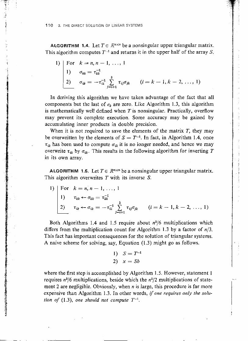
ALGORITH M 1.4. Let T E RnXn be a nonsingular upper triangular matrix. This algorithm computes T-l and returns it in the upper half of .the array S.

1) I For k = n , n - 1, . . . , 1

In deriving this algorithm we have taken advantage of the fact that all components but the last of ek are zero. Like Algorithm 1.3, this algorithm is mathematically well defined when T is nonsingular. Practically, overflow may prevent its complete execution. Some accuracy may be gained by accumulating inner products in double precision.

When it is not required to save the elements of the matrix T, they may be overwritten by the elements of S = T-l. In fact, in Algorithm 1.4, once tik has been used to compute aik it is no longer needed, and hence we may overwrite rik by oik. This results in the following algorithm for inverting T in its own array.

A LGORI'TH M 1.5. Let T E RnXn be a nonsingular upper triangular matrix. This algorithm overwrites T with its inverse S.

1) I For k = n , n - 1, . . . , 1

Both Algorithms 1.4 and 1.5 require about n3/6 multiplications which differs from the multiplication count for Algorithm 1.3 by a factor of n/3. This fact has important consequences for the solution of triangular systems. A naive scheme for solving, say, Equation (1.3) might go as follows.

where the first step is accomplished by Algorithm 1.5. However, statement 1 requires n3/6 multiplications, beside which the n2/2 multiplications of statement 2 are negligible. Obviously, when n is large, this procedure is far more expensive than Algorithm 1.3. In other words, if one requires only the solution of (1.3), one should not compute T-l.

1. TRIANGULAR MATRICES AND SYSTEMS 11 1

It should be stressed that the inverse of a matrix is seldom required in matrix computations. For whenever we are asked to compute

we can alternatively calculate the solution of

Such recasting of a problem can save a good deal of computations, as .the following examples show.

E X A M P LE 1.6. We wish to calculate the expression

where T is an upper triangular matrix of order n. Rather than inverting T, we may proceed as follows.

1) Solve the equation Tz = y

2) Calculate a = xTz

The naive way of computing a via T-l requires n3/6 multiplications to invert T, beside which the remaining calculations are insignificant. The alternative procedure, on the other hand, requires only n2/2 multiplications.

E X A M P L E 1.7. We wish to compute

where T is of order n and B E ItnXm. If we partition B and C by columns, then

( ~ 1 , c2, . . . , cm) = (T-lbl, T-lb2, . . . , T-lbm),

whence ci = T-lbi. Thus the columns of C can be found by solving the systems

Tci = bi (i = 1, 2, . . . , m).

If T is upper triangular, the naive computation requires n3/6 multiplications for .the inversion of T and another mn2/2 multiplications to compute C = T-lB, giving a total of (Qn + &m)n2 multiplications. The alternative procedure requires mn2/2 multiplications. Comparing these operation

6. Call a matrix of order n "upper Stieltjes of width k" if its nonzero elements lie on its diagonal and first k - 1 superdiagonals. Describe an efficient algorithm to invert an upper Stieltjes matrix U of width k ; to solve the equation Ux = b.

7. Equation (1.2) shows that (T[")-l may be easily calculated from (TLk-I])-1. Describe an algorithm that computes T-l by computing successively (TI1])-l, (T[23)-1, . . . , (TIn])-l = T-l.

8. A matrix T is block upper triangular if it can be partitioned in the form


counts, we see that the procedure involving T-I always requires more work than the alternative procedure, although the difference becomes negligible for in > n.

EXERCISES

1. Show that if T = D - U, where D is a nonsingular diagonal matrix of order iz and U is a strictly upper triangular matrix, then

2. Describe an equivalent of Algorithm 1.1 for solving lower triangular systems.

3. Describe an equivalent of Algorithm 1.4 for inverting lower triangular matrices.

4. Write an INFL program to generate the inverse of an upper triangular matrix T row-wise. [Hint: Solve the systems skTT = ekT (k = 1, 2, . . . , n).]

5. A lower triangular matrix is a Stieltjes matrix if its nonzero elements lie on its diagonal and first subdiagonal. Describe an efficient algorithm for inverting a lower Stieltjes matrix L; for solving the system Lx = b.

where each diagonal block Ti, is square. Prove that T is nonsingular

2. GAUSSIAN ELIMINATION 11 3

if and only if its diagonal blocks are nonsingular, and that its inverse is block triangular with the same partitioning. Assuming that the matrices Tzl are known, generalize Algorithm 1.5 to find the inverse of a block upper triangular matrix. Give two INFL descriptions: one in terms of blocks and the other in terms of elements.

2. GAUSSIAN ELIMINATION

[n this section we shall give algorithms for reducing a matrix to upper trapezoidal form. The basic algorithm, called Gaussian elimination, mim- ics the process of eliminating unknowns from a system of linear equations. As such it provides a direct method for solving linear equations. Moreover, the algorithms may be described in terms of matrix operations, and these descriptions in turn lead to the factorizations to be described in Section 3. + To illustrate these ideas we consider the following system of linear equations

261 462 - 263 = 6

6 6 2 + 5 6 3 = 0 . (2.1)

461 + 6 2 - 263 = 2

If 4 times the first equation is subtracted from the second and 2 times the first subtracted from the third, the result is the system

in which the variable 6, does not appear in the second and third equations. Likewise the variable 6, can be eliminated from the third equation by subtracting 713 times the second equation from the third to obtain

The system (4.3) is upper triangular and can be solved by the techniques of Section 1. Obviously this idea of elimination can be extended to give a

1 14 3. THE DIRECT SOLUTION OF LINEAR SYSTEMS

j general method for solving systems of any order. However, there is more to the process than this.

Let A = A,, A,, and A, be the matrices of the systems (2. I), (2.2), and (2.3), respectively; e.g.,

Then A, is obtained from A, by subtracting + the first row of A, from the 1 second row and 2 times the first row from the third. From the discussion of matrix multiplication in Section 1.4, we know that A, can be obtained by premultiplying A, by a suitable matrix, and in fact it is easy to verify that

A2 = MIA,, 1 ,

where

Similarly

where

Combining (2.4) and (2.5), we see that

Thus to solve the system Ax = b we need only calculate the vector c = MlM2b and solve the upper triangular system

Moreover, the expression (2.6) can be rearranged to give a factorization of A into a lower and upper triangular matrix. Since the Mi are nonsingular, we have from (2.6)

A = M;lM<lA3. (2.7)

2. GAUSSIAN ELIMINATION 115

Since MI and M, are unit lower triangular, so is the product of their inverses. Hence, if we set L - M;I M;l and U = A,, Equation (2.7) becomes

1, 1 A = LU,

where L is unit lower triangular and U is upper triangular. Since

I DEFINITION 2.1. An elementary lower triangular matrix of order n and index k is a matrix of the form

T M = I, -mek ,

,

1 d

where eiTm = O (i = 1 , 2, . . . , k). (2.8)

1 0 0 M ; ~ = (; 1 0

M i l = ( ; ; ;), 4

The conditions (2.8) say that the first k components of rn are zero; that is, m has the form m = (0 ,0 , . . . , 0 , p,+, , p,,,, . . . , P , ) ~ . In general an

I elementary lower triangular matrix has the form

1 L is itself the product of very simple triangular matrices. 1 Obviously the above discussion depends critically on the matrices Mi, 1 which are called elementary lower triangular matrices. We begin our

formal exposition of Gaussian elimination with a discussion of their prop- I I erties.

Elementary lower triangular matrices are easily inverted.

M =

' 1 0 ... 0 . . . 0 '

0 1 . * . 0 ... 0 . . . . . . 0 0 ... 1 ... 0 .

0 0 - . . -Pk+l ' ' ' 0 . . . . . .

-0 0 ... -pn ... 1, r'

Thus an elementary lower triangular matrix is an identity matrix with some additional nonzero elements in the kth column below the diagonal.

T' 1 I 7


THEOREM 2.2. Let M = I - nzeJCT be an elementary lower triangular matrix. Then

M-l = I + mekT.

i PROOF. Let X = I + mekT. Then

i ! Since M is an elementary lower triangular matrix, ekTm = 0. Hence MX = 1 1 I and X is the inverse of M.

The computational significance of elementary lower triangular matrices I I

1 is that they can be used to introduce zero components into a vector. 1 * I

THEOREM 2.3. Let ekTx = fk # 0. Then there is a unique elementary I lower triangular matrix M of index k such that I

1 MX = (61, f 2 , . . , fk, O,O, . . . , O)T. (2.9) t t

1 PROOF. We seek M in the form M = I - mekT. Since M is to be of index k, we must have

I

I 1 !

Now

p i = 0 ( i = l , 2 , . . . , k).

MX = ( I - nzekT)x = x - (ekTx)m.

I Since the last n - k components of MX are to be zero, we must have

r

f i - 5 ; p i = 0 ( i = k + l , k + 2 , . . . , n),

and if fk # 0,

f i Eli = - ( i = k + l , k + 2 , ..., n). (2.1 1)

6 k

Thus if M exists, it is uniquely determined by (2.10) and (2.1 1). On the other hand, if 5;, # 0, then the vector m can be determined from (2.10)


and (2.1 I), and it is easy to verify that the associated matrix M = I - mekT satisfies (2.9).

Thus when f k # 0, we can multiply x by an elementary lower triangular matrix chosen so that the last n - k components of x are replaced by zeros and the other components are left unaltered. When 5;, = 0, such a matrix does not exist, unless &+, , . . . , f , are also zero, in which case any elementary lower triangular matrix of index k will do the job. I t should be noted that Equations (2.10) and (2.11) define an algorithm for computing rn and hence M.

In the method of Gaussian elimination for reducing a matrix to upper trapezoidal form, the matrix is premultiplied by a sequence of elementary lower triangular matrices, each chosen to introduce a column with zeros below the diagonal. The method revolves around Theorem 2.3, which allows us to calculate the necessary elementary lower triangular matrices. It should

,, be stressed that any class of matrices satisfying something like Theorem 2.3 can be used for the reduction: the elementary lower triangular matrices are used here because they are easy to compute and multiply. An important alternative will be discussed in Chapter 5.

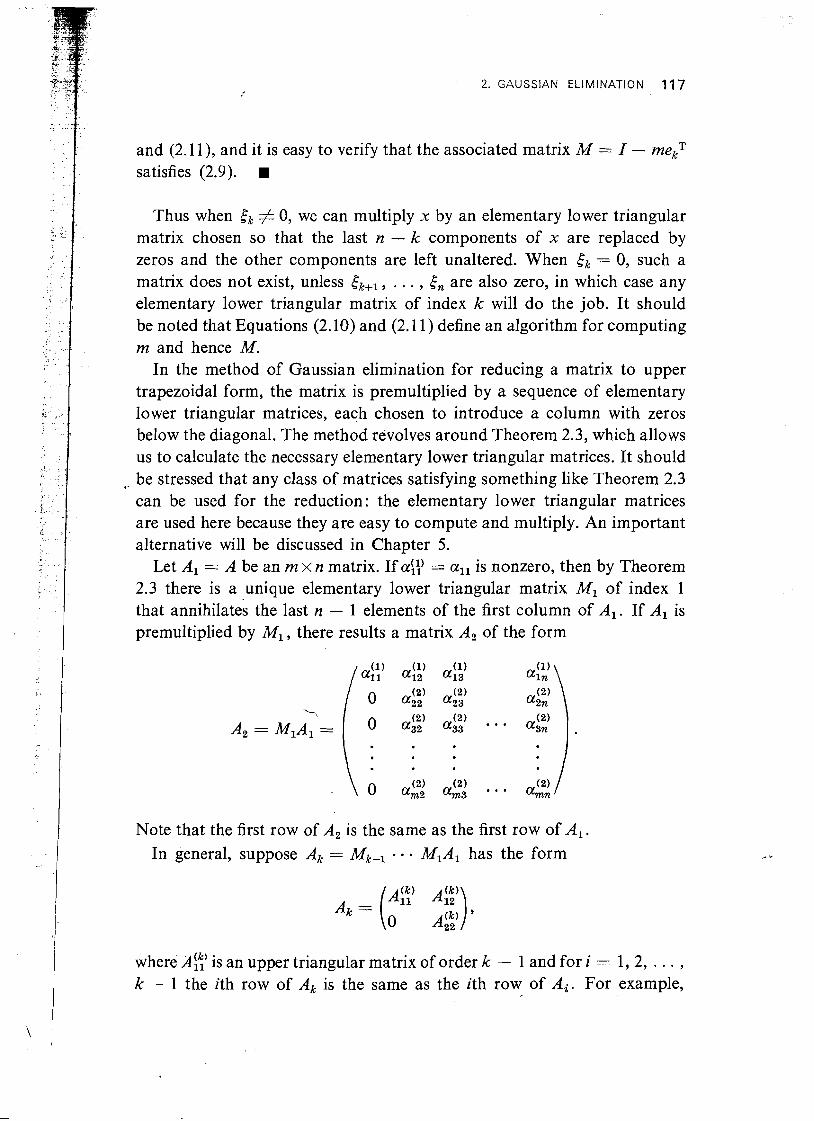
Let A, = A be an m x n matrix. If a!;) = all is nonzero, then by Theorem 2.3 there is a unique elementary lower triangular matrix MI of index 1 that annihilates the last n - 1 elements of the first column of A, . If A, is premultiplied by M I , there results a matrix A, of the form

Note that the first row of A, is the same as the first row of A,. In general, suppose Ak = Mk-l MIA1 has the form

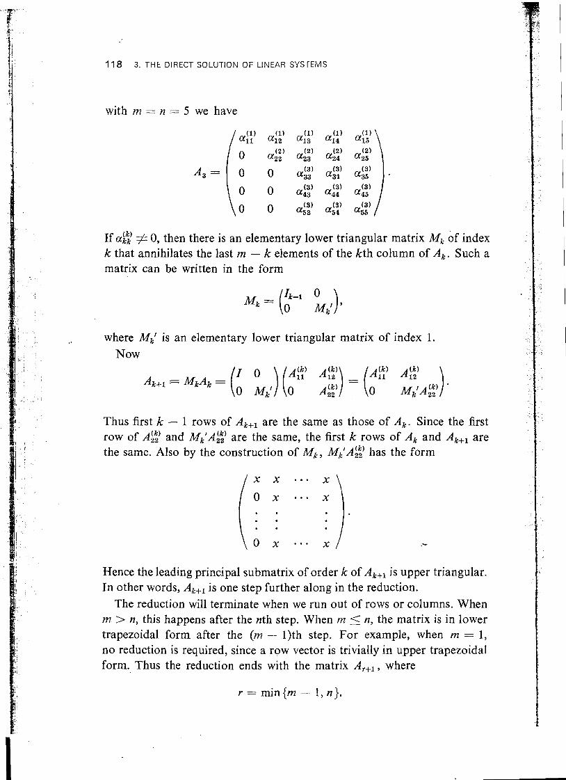
where A::' is an upper triangular matrix of order k - 1 and for i = 1,2, . . . , k - 1 the ith row of Ak is the same as the ith row of A i . For example,


with m = n = 5 we have

If a;:) # 0, then there is an elementary lower triangular matrix Mk of index k that annihilates the last rn - k elements of the kth column of A,. Such a matrix can be written in the form

where Mkl is an elementary lower triangular matrix of index 1. Now

Thus first k - 1 rows of A,,, are the same as those of A,. Since the first row of A::' and M,'A::' are the same, the first k rows of Ak and A,,, are the same. Also by the construction of Mk, M~'A:~) has the form

Hence the leading principal submatrix of order k of A,,, is upper triangular. In other words, A,,, is one step further along in the reduction.

The reduction will terminate when we run out of rows or columns. When m > n, this happens after the nth step. When m _( n, the matrix is in lower trapezoidal form after the (m - 1)th step. For example, when m = 1, no reduction is required, since a row vector is trivially in upper trapezoidal form. Thus the reduction ends with the matrix A,,, , where

r = min(m -. 1, n).


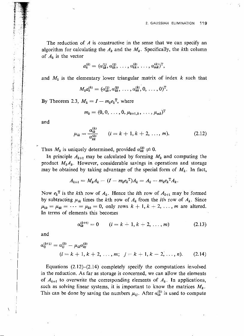
The reduction of A is constructive in the sense that we can specify an algorithm for calculating the Ak and the Mk. Specifically, the kth column of Ak is the vector

l and Mk is the elementary lower triangular matrix of index k such that

; / Thus Mk is uniquely determined, provided a$ # 0.

. -

,k

I In principle Akfl may be calculated by forming Mk and computing the product MkAk. However, considerable savings in operations and storage

M ~ ~ L ~ ' = ( 0 , a:, . . . , akk, ( k ) 0 , . . . , o ) ~ .

By Theorem 2.3, Mk = I - mkekT, where

and

I may be obtained by taking advantage of the special form of Mk. In fact,

I

mk = (0, 0, - . 0, Pkkf1.k , - I U ~ ~ ) ~

I- ( k )

(nik Pik = - ( i = k + 1 , k + 2 , ..., m).

afckk) (2.12)

Now ekT is the kth row of Ak. Hence the ith row of Ak+, may be formed by subtracting p, times the kth row of Ak from the ith row of A,. Since ,ulk = ,u2k = = pkk = 0, only rows k + 1, k + 2, . . . , m are altered. In terms of elements this becomes

l and

!k+l' - ( k ) - ( k ) a, - aij Pikakj

( i = k + l , k + 2 , . . . , m ; j = k + l , k + 2 ; . . . , n). (2.14)

Equations (2.12)-(2.14) completely specify the computations involved in the reduction. As far as storage is concerned, we can allow the elements of Ak+, to overwrite the corresponding elements of Ak. In applications, such as solving linear systems, it is important to know the matrices M k . This can be done by saving the numbers p i j . After a$' is used to compute


p,, it is not used again, and in fact it is reduced to zero in the transforma- tion from Ax: to A k f l . Hence, if we agree to store only the nonzero entries of A,,, , the number pik may be placed in the location originally occupied by a i k .

These considerations may be summed up in the following algorithm.

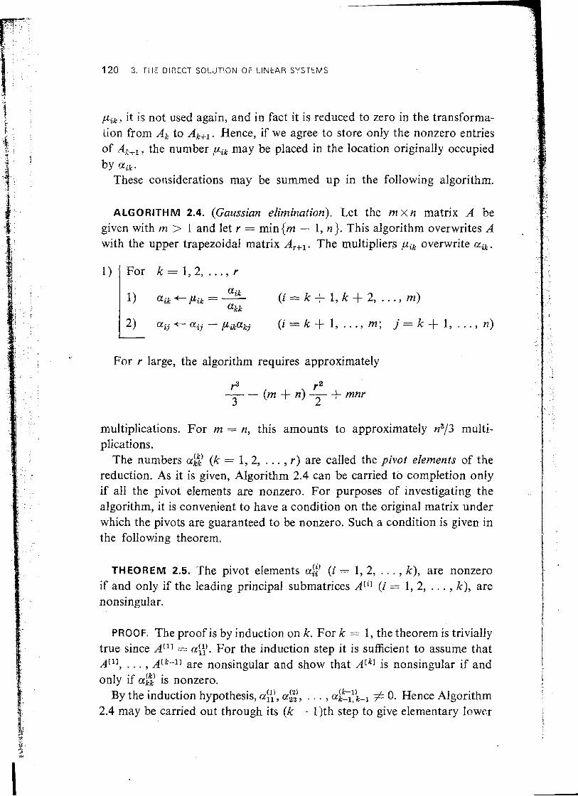
ALGORITHM 2.4. (Gaussian elimination). Let the m x n matrix A be given with m > 1 and let r = min(m - 1, n). This algorithm overwrites A with the upper trapezoidal matrix A,,,. The multipliers pik overwrite aik.

1) For k = 1,2, ..., r aik

I) aik +- pik = - ( i = k + l , k $ 2, . . . , m) akk

For r large, the algorithm requires approximately

multiplications. For m = n, this amounts to approximately n3/3 multiplications.

The numbers a;;) (k = 1, 2, . . . , r ) are called the pivot elements of the reduction. As it is given, Algorithm 2.4 can be carried to completion only if all the pivot elements are nonzero. For purposes of investigating the algorithm, it is convenient to have a condition on the original matrix under which the pivots are guaranteed to be nonzero. Such a condition is given in the following theorem.

THEOREM 2.5. The pivot elements a::' (i = 1, 2, . . . , k), are nonzero if and only if the leading principal submatrices ALil (i = 1, 2, . . . , k), are nonsingular.

PROOF. The proof is by induction on k. For k = 1, the theorem is trivially true since AL11 = a!?. For the induction step it is sufficient to assume that ALII , . . . , ALk-l1 are nonsingular and show that ALkl is nonsingular if and

only if a;;) is nonzero. (k-1) By the induction hypothesis, a::', ak), . . . , a,,, # 0. Hence Algorithm

2.4 may be carried out through its (k - 1)th step to give elementary 1ewc.r

triangular matrices

2. GAUSSIAN ELIMINATION

n/ri of index i (i = 1, 2, . . . , k - 1) such that

(k-1) where A!:) is upper triangular with diagonal elements a::), . . . , ak-l,k-l. It follows that A;~] is upper triangular with diagonal elements a g , . . . ,

(k-1) (k) . (1) (k-1) ak-1, k-1, a k k . Since all , . . , ak-1, k-1 # 0, is nonsingular if and only if afC2 is nonzero. Now since MI , . . . , Mk-, are lower triangular, A;~]

Ckl = M~-, . M:~]A[~ I (Exercise 1.4.18). Since M, is unit lower triangular, so is M:~'. Thus is nonsingular if and only if A;~] is nonsingular, which, we have seen, is true if and only if a$) # 0. w

Carried through its kth step, the method of Gaussian elimination pro-

* L duces elementary lower triangular matrices Mi of index i (i = 1,2, . . . , k)

-' ,. . 1 re-

Y d.such that A,+, = MkMk-, . . MIA is zero below its first k diagonal ele- I , I

- I%

2, . . . , k).

ments. Once started, the method proceeds deterministically, provided the pivots are nonzero. This suggests that the matrices MI , M,, . . . , Mk are uniquely determined by the requirement that MkMkP1 . . . MIA be zero

f

PROOF. The proof is by induction on k. For k = 1, Ml and N1 are elementary lower triangular matrices of index 1 that introduce zeros into the last rn - 1 elements of the first column of A. Since all # 0, this requirement uniquely determines MI and Nl (Theorem 2.3) which are thereby equal.

For the induction step, assume that All], . . . , Ark] are nonsingular and that Mk . . . MIA and Nk NIA are both zero below their first k diagonal elements. Since Mk is an elementary lower triangular matrix of index k, so is M;l, and it is easily verified that

\

below its first k diagonal elements. The following theorem shows that this is indeed the case.

THEOREM 2.6. Let A E RmXn and suppose that A['], AC2], . . . , ACkl are nonsingular. For i = 1,2, . . . , k let Mi and Ni be elementary lower triangular matrices of index i. If MkMk-l - MIA and NkNk-, . NIA are both zero below their first k diagonal elements, then Mi = Ni (i = 1,

.is zero below its first k - 1 diagonal elements. Likewise NkP1 . . NIA is


zero below its first k - 1 diagonal elements. By the induction hypothesis Mi = N,: ( i 1 2 , . . . , k - 1 ) Hence Mk-, MIA = Nk-, NIA = A,, where A, is the matrix resulting from k - 1 steps of Gaussian elimination. By Theorem 2.5, a:;) # 0. Hence Mk and Nk are the unique elementary lower triangular matrices of index k that introduce zeros below the kth diagonal of Ak. It follows that Mk = Nk. .

Algorithm 2.4 breaks down at step 1.1 when the pivot ukk = 0. If some aik # 0 (i = k + 1, . . . , m), then the reduction cannot be continued. However, if a, = 0 (i = k + 1, . . . , m), then Ak is already zero below its kth diagonal element, and any elementary lower triangular matrix of index k can be used for Mk, thus if a zero pivot emerges at step k, it may be possible to continue the reduction, but Mk, Mk+,, . . . , M, are no longer unique.

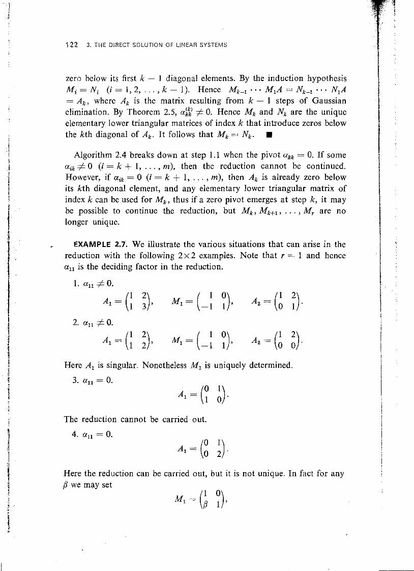
EXAMPLE 2.7. We illustrate the various situations that can arise in the reduction with the following 2 x 2 examples. Note that r = 1 and hence a,, is the deciding factor in the reduction.

1. a,, # 0.

Here A, is singular. Nonetheless MI is uniquely determined.

The reduction cannot be carried out.

Here the reduction can be carried out, but it is not unique. In fact for any i i

B we may set


giving

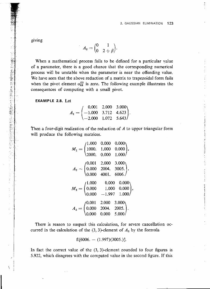
When a mathematical process fails to be defined for a particular value of a parameter, there is a good chance that the corresponding numerical process will be unstable when the parameter is near the offending value. We have seen that the above reduction of a matrix to trapezoidal form fails when the pivot element a;;) is zero. The following example illustrates the consequences of computing with a small pivot.

EXAMPLE 2.8. Let 0.001 2.000 3.000

-1.000 3.712 4.623 -2.000 1.072 5.643

hen a four-digit realization of the reduction of A to upper triangular form will produce the following matrices.

There is reason to suspect this calculation, for severe cancellation oc- curred in the calculation of the (3, 3)-element of A, by the formula

In fact the correct value of the (3, 3)-element rounded to four figures is 5.922, which disagrees with the computed value in the second figure. If this

,124 3. THE DIRECT SOLUT~ON OF LINEAR SYSTEMS

computed value is used in subsequent calculations, the results will in general be accurate to only one or two figures.

The above example suggests that the emergence of a small pivot in the course of Algorithm 2.4 may be a harbinger of disaster. If the problem at hand requires the matrices M,, M,, . . . , M,, A,+, , there is very little that can be done other than redoing the calculations in higher precision. However, in many applications the reduction is an intermediate step in the solution of a larger problem and it may be possible to rearrange the problem so that the reduction is performed on a different matrix, one for which no small pivots emerge. For example, suppose the matrix in Example 2.8 had arisen in connection with solving the linear system

If the first and second equations are interchanged, there results a linear system whose matrix

-1.000 3.712 4.623 0.001 2.000 3.000

-2.000 1.072 5.643

can be reduced without difficulty. The above considerations suggest that we modify Algorithm 2.4 to avoid

small pivotal elements by interchanging the rows and columns of the matrix A. Specifically, if at the kth stage of the reduction, the element a:;) is unsatisfacto~ily small, we may choose some other element, say (k) # 0, as the pivot. If we interchange rows k and ek and then columns aek9 yk

k and yk, the result is to move into the (k, k)-position, and the reduction may be continued with the new pivot. Obviously we must have ek > k and yk > k, otherwise the interchanges will disturb the zeros previously introduced by the reduction.

In matrix terms the modified algorithm may be described as follows. At the kth stage, A, is premultiplied and postmultiplied, respectively, by the elementary permutations ik,Qk and (cf. Example 1.4.26), and then premultiplied by an elementary lower triangular matrix M, of index k chosen to introduce a new column of zeros. Thus


For simplicity of notation, we shall denote the elementary permutation and by Pk and Qk, respectively, so that

The incorporation of interchanges into Algorithm 2.4 complicates the expression for Ak. It might be thought that it would be considerably more difficult to analyze the modified algorithm. Fortunately, as the following theorem shows, the modified algorithm is equivalent to making all the interchanges first and then applying Algorithm 2.4. Of course in practice we must make the interchanges as we go along, since there is no way to know if a pivot is zero until it has been computed; but for -theoretical purposes (say a rounding-error analysis) we may assume that all the interchanges have already been performed.

THEOREM 2.9. Let the modified algorithm be applied to A producing matrices Qi, Pi , Mi, and A,,, (i = 1, 2, . . . , k). Let

A' = PkPk-, . PlAQlQ2 . - . Qk.

Then Algorithm 2.4 can be applied to A' through its kth step. If Mi' and

I A:,, (i = 1, 2, . . . , k), are the matrices produced by Algorithm 2.4, then

and Mi' = PkPk-, . . . Pi+lMiPi+l ' ' ' Pk-,Pk.

PROOF. From Equation (2.15) it follows that

Because Pi2 = I, this equation is equivalent to

Ak+, = Mk'Mi-l . M1'Ar, (2.17)

where Mi' is defined by (2.16). Now it is easily verified that if Mk is an elementary lower triangular matrix of index k and i, j > k, then IijMkIii is also an elementary lower triangular matrix of index k. It follows that Mi' is an elementary lower triangular matrix of index k. The first k diagonal

1 elements of Ak+, are nonzero and hence the first k leading principal sub- !

\ I matrices of A' are nonsingular. Thus by Theorem 2.6, MIf, M2', . . . , M,', and Ak+l are the result of applying k steps of Algorithm 2.4 to A'. H


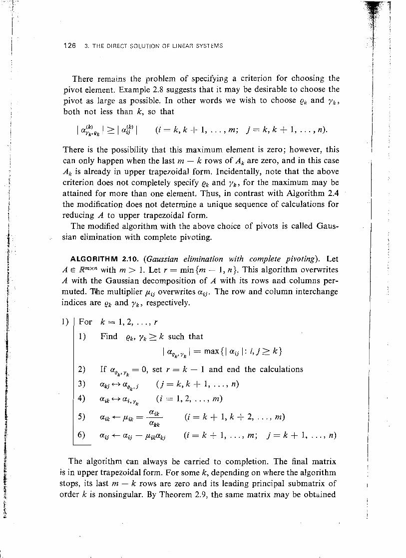
There remains the problem of specifying a criterion for choosing the pivot element. Example 2.8 suggests that it may be desirable to choose the pivot as large as possible. In other words we wish to choose ek and yk, both not less than k, so that

( k ) 1 ayk*ek 1 1 1 ( i = k , k + l , . . . , m; j = k , k + l , . . . , n).

There is the possibility that this maximum element is zero; however, this can only happen when the last m - k rows of Ak are zero, and in this case Ak is already in upper trapezoidal form. Incidentally, note that the above criterion does not completely specify ek and yk, for the maximum may be attained for more than one element. Thus, in contrast with Algorithm 2.4 the modification does not determine a unique sequence of calculations for reducing A to upper trapezoidal form.

The modified algorithm with the above choice of pivots is called Gaus- . sian elimination with complete pivoting.

ALGO RlTH M 2.1 0.. (Gaussian elimination with complete pivoting). Let A E Rmxn with m > 1. Let r = min {m - 1, n}. This algorithm overwrites A with the Gaussian decomposition of A with its rows and columns permuted. T%e multiplier pij overwrites aij . The row and column interchange indices are ek and yk, respectively.

' For k = 1,2, ..., r

1) Find ek, yk 2 k such that

I a997k 1 = max{I aij 1 : i , j > k}

2) If aQk, yk = 0, set r = k - 1 and end the calculations

3) akj+-+aek,j ( j = k , k + l , . . . , n)

4) a, +-+ ai, yk (i = 1,2, . . ., m)

The algorithm can always be carried to completion. The final matrix is in upper trapezoidal form. For some k, depending on where the algorithm stops, its last m - k rows are zero and its leading principal submatrix of order k is nonsingular. By Theorem 2.9, the same matrix may be obthined


by applying k steps of Gaussian elimination to the A with its rows and columns suitably permuted. Thus Gaussian elimination with complete pivoting is a procedure for calculating the decomposition described in ,the following theorem.

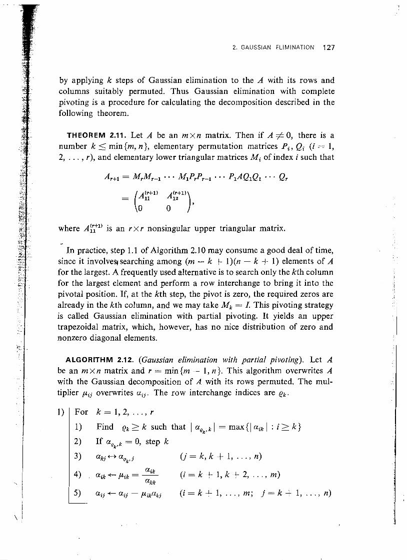
THEOREM 2.11. Let A be an m x n matrix. Then if A # 0, there is a number k _( min {m, n), elementary permutation matrices P i , Qi (i = 1, 2, . . . , r), and elementary lower triangular matrices Mi of index i such that

where AF" is an r x r nonsingular upper triangular matrix.

In practice, step 1.1 of Algorithm 2.10 may consume a good deal of time, since it involveqsearching among (m - k + l)(n - k -1- 1) elements of A for the largest. A frequently used alternative is to search only the kth column for the largest element and perform a row interchange to bring it into the pivotal position. If, at the kth step, the pivot is zero, the required zeros are already in the kth column, and we may take Mk = I. This pivoting strategy is called Gaussian elimination with partial pivoting. It yields an upper trapezoidal matrix, which, however, has no nice distribution of zero and nonzero diagonal elements.

A LGO RlTH M 2.1 2. (Gaussian elimination with partial pivoting). Let A be an m x n matrix and r = min {m - 1, n). This algorithm overwrites A with the Gaussian decomposition of A with its rows permuted. The multiplier pij overwrites uij. The row interchange indices are ek.

For k = l ,2 , . . . , r

1) Find p k 2 k s u c h that I aek ,k I=max{ la ik : i > k )

2) If aek,, = 0, step k

3, a k j t t a q , j ( j = k , k + 1, . . . , n)

aik 4, . a i k + pik = - ( i = k + 1 , k + 2 , . . . , m )

a k k

5) a i j+a . z j - ~ i k a k j ( i = k + l , . . . , m; j = k $ 1 , . . . , n)


THEOREM 2.13. Let A be an m x n matrix and let r = min(m - 1, n) . Then there are elementary permutations Pi (i = 1,2, . . . , r), and elementary lower triangular matrices ,Mri of index i (i = 1, 2, . . . , r), such that

is upper trapezoidal.

EXERCISES

I'! Let L E Rnxn be unit lower triangular, and let M, be the elementary lower triangular matrix of index k whose kth column is the same as the kth column of L. Show that L = M1M2 . Mn-,. Apply Theorem 2.2 to derive algorithms for inverting L and for solving the system Lx = b. How are these algorithms related to those of Exercises 1.2 and 1.3?

2. Let M be an elementary lower triangular matrix of index k and let i, j > k. Show that M' = ZijMlij is also an elementary lower triangular matrix of index k. How is M' obtained from M?

3. Let A, M E Rnxn with M an elementary lower triangular matrix of index 1. Give efficient INFL algorithms for overwriting A with AM-l, AMT, MAM-l, and MAMT.

4. Define the notion of an elementary upper triangular matrix of order n in a suitable way. Describe the important properties of such matrices.

5. Describe how a matrix can be reduced to lower trapezoidal form by postmultiplication by elementary upper triangular matrices. Give an INFL algorithm implementing this variation of Gaussian elimination. Discuss the incorporation of interchanges into the algorithm.

6. Give an efficient INFL program for reducing an upper Hessenberg matrix to upper triangular form by Gaussian elimination with partial pivoting.

7. Give an efficient INFL program for reducing a tridiagonal matrix to upper triangular form by Gaussian elimination (note that the result is Stieltjes matrix). Do the same for Gaussian elimination with partial pivoting. (The result is a Stieltjes matrix of width 3.) Also give algorithms in which the elements are suitably stored in linear arrays.

EXERCISES 129

8. Give an efficient INFL program for reducing a band matrix of width 2k + 1 (cf. Exercise 1.3.6) to upper triangular form by Gaussian elimination with partial pivoting. i

9. Let A be symmetric with all # 0. After one step of Gaussian elimination A has the form

( 2 1 ;2T).

Show that +, is symmetric.

10. Give an efficient INFL algorithm for reducing a symmetric matrix A to upper triangular form by Gaussian elimination. Assume that only the upper half of the matrix A is present in the array A. Do the same for a symmetric band matrix of width 2k + 1.

11. The matrix A E Rnxn is diagonally dominant if 1 aii ( > xj$i 1 aij 1 (i = 1,2, . . . , n). Prove that

1. if A is diagonally dominant, then any principal submatrix of A is diagonally dominant, 2. if A is diagonally dominant, then A is nonsingular.

Conclude that Algorithm 2.4 will not fail when applied to a diagonally dominant matrix.

12. Let A be diagonally dominant and after one step of Gaussian elimination let A have the form

( 2 1 2;). Prove that A, is diagonally dominant. Conclude that for symmetric, diagonally dominant matrices Gaussian elimination and Gaussian elimination with partial pivoting amount to the same thing.

13. Describe how Gaussian elimination may be used to compute the decomposition of Theorem 1.7.1. (Note that as a practical procedure this approach has the drawback that one must be able to recognize when a number that has been contaminated by rounding error is zero.)

14. An elementary R-matrix of index k is a matrix of the form R = I - rekT, where ekTr = 0. Prove that

(There is no standard terminology for such matrices.)


I 15. Prove that 'if ekT.u f 0, then there is an elementary R-matrix of

., index k such that i

where Dk+, is diagonal of order k. Thus An+, is diagonal. Give an INFL program implementing this Gauss-Jordan reduction of A to diagonal form.

RX = tk% = (0, . . . , 0 , tk, 0, . . . ,O)T. 4

1 17. Show that the matrices A:?' in the Gauss-Jordan reduction are the same as the corresponding matrices resulting from Gaussian elimination. Hence derive conditions under which the Gauss-Jordan reduction can be carried to compIetion.

16. Gauss-Jordan reduction. Let A E PXn. Determine elementary R- matrices Ri of index i such that A,+, = RkRk-, - . . RIA has the form

18. What kind of interchange strategies may be incorporated into the Gauss-Jordan reduction ?

j

19. Strictly speaking, Algorithm 2.12 does not produce the Gaussian decomposition sf A with its rows permuted, since the multipliers pij do not appear in the correct order. Modify the algorithm so that the pij do appear in the correct order. [Hint: only one minor change in one statement is required. ]

20. The necessity of actually interchanging rows in Algorithm 2.12 can be circumvented by the following trick. Initialize an index vector I with the values A, = 1, A, - 2, . . . , A, = n. Whenever a row interchange is required, interchange instead the corresponding components of I. Replace all references to aij by references to a ~ ~ , ~ . Give INFL code for this variant of Algorithm 2.12. Discuss the situation of the multipliers (cf. Exercise 2.19). Is there any significant difference in work between this variant and Algorithm 2.12?

F 21. Devise a variant of Algorithm 2.10 that avoids interchanges.

NOTES AND REFERENCES

1 ? A variant of Gaussian elimination for systems of order three appears in the Chinese work "Chiu-Chang Suan-Shu," composed about 250 B.C.

I

3. TRIANGULAR DECOMPOSITION 131

[see Boyer (1968, page 219)l. The method is readily motivated in terms of systems of linear equations, and in one form or another it often appears in linear algebra texts. Unfortunately many of these texts fail to describe the pivoting strategies that are so necessary to the numerical stability of the methods.

The point of view taken here in which Gaussian elimination is regarded as being accomplished by premultiplications by elementary lower triangular matrices originated with Turing (1948) and has been extensively exploited by Wilkinson (AEP, for example). This approach has the advantage of generalizing readily; any other computationally convenient class of matrices may be used to introduce zeros.

Elementary lower triangular matrices are a special case of a class of matrices that differ from an identity matrix by a matrix of rank unity. Householder (1964) calls all such matrices elementary matrices and shows how many of the transformations used in numerical linear algebra may be reiiuced to multiplications by elementary matrices.

Gaussian elimination lends itself naturally to the reduction of matrices with special distributions of zeros such as tridiagonal matrices, for it is easy to see what the pivoting and elimination operations will do to the zero elements. Martin and Wilkinson (1967, HACLA/I/6) give algorithms for efficiently reducing band matrices.

A natural extension of Gaussian elimination is to eliminate all the off- diagonal elements in a column at each step, which will finally yield a diagonal matrix. This method is known as the Gauss-Jordan method [the associa- tion of Jordan with the method is apparently a mistake; see Householder (1964, page 141)l. In most applications this method is unnecessarily expensive; however, Bauer and Reinsch (HACLA/I/3) have used it to invert positive definite matrices.

An excellent introduction to Gaussian elimination, as well as other algorithms in this chapter, has been given by Forsythe and Moler (1967).

3. TRIANGULAR DECONl POSITION

In this section we shall consider algorithms for factoring a square matrix A into the product LU of a lower and an upper triangular matrix. Such a factorization is often called an LU decomposition of the matrix A. Since an LU decomposition expresses a matrix as the product of simpler matrices, it can be used to simplify calculations involving the matrix. For example, in the unlikely event that the inverse of A is required, it can be computed

in the form A-l = U-lL-I by the techniques of Section 3.1. Throughout this section we shall assume that A is a square matrix of order n ; however, some of the results may easily be generalized to rectangular matrices.

Actually we have already seen a method for computing an L U factorization of A, for if Gaussian elimination is applied to A, the result is a sequence MI, M,, . . . , M,-, of unit lower triangular matrices such that

is upper triangular. If we set

then L is unit lower triangular and A = LA,. Moreover, it is easy to verify that

L r

where the pij are multipliers produced by Algorithm 2.4. Thus Algorithm 2.4 can be regarded as an algorithm for overwriting A with an L U decomposition, L being stored in the lower part of the array A and U = A, in the upper part.

The close connection of Gaussian elimination with an L U decomposition of A raises the question of the existence and uniqueness of such decompositions; for we have seen that the Gaussian decomposition may fail to exists or be unique. There is, in general, no unique L U factorization of a matrix. If A = L U is an L U factorization of A and D is a nonsingular diagonal matrix, then L' = LD is lower triangular and U' = D-'U is upper triangular. Hence

A = L U = LDD-'U = L'U',

and L'U' is also an L U decomposition. This example suggests the possibility of normalizing .the L U decompositions of a matrix by inserting a diagonal matrix. We shall say that

A = LDU

is an LD'U decomposition of A provided that L is unit lower triangular, D is diagonal, and U is unit upper triangular. The question of the existence


and uniqueness of LDU decompositions may be answered in terms of the leading principal submatrices of A.

THEOREM 3.1. Let A E Rnxn. Then A has a unique LDU decomposition if and only if Ar11, A['] , . . . , AIn-l1 are nonsingular.

PROOF. We prove the theorem under the hypothesis that A is nonsingular, leaving the case of singular A as a (rather difficult) exercise.

We first show that if A has an LDU decomposition, then it is unique. Let A = LIDIUl and A = L2D2U2 be LDU decompositions of A. Since A is nonsingular, so are Dl and D,. From the equation LIDIUl = L,D,U,, it follows that

L,lL1 = D,U,UY~D,~ . (3.2)

Now the left-hand side of (3.2) is a unit lower triangular matrix and the right-hand side is an upper triangular matrix. Hence both sides are an identity matrix. This means L;lL1 = I or L1 = L, . A similar argument shows that Ul = U , . Finally, since L1 and Ul are nonsingular, the equation LIDIUl = LID2 Ul implies that Dl = D, .

It remains to show that A has an LDU decomposition if and only if AI1l, . . . , AIn-l1 are nonsingular. First suppose that A = LDU is an LDU decomposition of A. Then L, D, and U are nonsingular. Since L and U are triangular and D is diagonal, LLkl, DIkl, and UIkl are nonsingular. However, AIkl = L[klD[kIU[kI, hence AIk1 is nonsingular.

Conversely, suppose that AC1], A12] , . . . AIR-11 are nonsingular. Then by Theorem 2.5 the algorithm of Gaussian elimination can be carried to completion and we can write A = LA,, where L is given by (3.1). Now the diagonal elements of A, are the pivot elements a;:) (k = 1,2, . . . , n), which by Theorem 2.5 are nonzero. Let D = diag(a\y, ag2,), . . . , ah%) and let U = D-lA, . Then A = LDU is an LDU decomposition of A.

From the proof of Theorem 3.1 it is evident that when an LDU decomposition exists, its elements can be written in terms of the quantities calculated by Algorithm 2.4. Specifically,

6. = (i) z aii (i = 1, 2, . . ., n),


We now turn to the description of algorithms for computing LU decompositions of a nonsingular matrix. Different LU decompositions may be obtained by treating the diagonal in the LDU decomposition differently. There are three important variants. The first associates D with the lower triangular part to give the factorization

where L is lower triangular and U is unit upper triangular. This can be accomplished as follows. In terms of scalars, Equation (3.4) can be written

A = L'U = (LD)U.

This is known as the Crout decomposition. The second, called the Doolittle decomposition, associates D with the upper triangular part

A = LU' = L(DU).

When A is symmetric and has a unique LDU decomposition, the decomposition must have the form

If the diagonal elements of D are positive, then we can form the matrix DY2 = diag(8:/12, . . . , @/n2). Thus A can be written as

This third variant is known as the Cholesky decomposition of A. Any of these three decompositions can be calculated by performing the

Gaussian reduction on A and using (3.3) to calculate the LDU decomposition (in fact, Gaussian elimination gives the Doolittle decomposition immediately). However, there are practical advantages to having algorithms that compute the decompositions directly. We shall confine our discussion to the Crout and Cholesky decompositions.

In the Crout reduction, we seek a factorization of the form

A = LU, (3.4)

min(i,j} orij = C liplj (i, j = 1, 2, . . . , n).

1-1

In particular, since vll = 1,

oril = lilvll = Ail (i = 1, 2, . . , n). (3.6)

Moreover


so that a1 j

vlj = - ( j = 2, 3, . . . , n). 211

Equations (3.6) and (3.7) determine the first column of L and the first row of U.

Now suppose that the first k - 1 columns of L and the first k - 1 rows of U have been computed. Then since vkk = 1 ,

whence k-1

Aik = aik - z Ailvlk (i = k, k + 1, . . . , n). 1=1

(3.8)

Similarly

v k j = = q a k j - gl ~ k ~ l j ) ( j = k + 1, . . . , n).

Equations (3.8) and (3.9) express the elements of the kth column of L and the kth row of U in terms of known quantities.

Concerning the organization of storage, note that after aij is used to compute Aij or vi j , whichever, it is no longer used. Hence the nonzero elements of L and U can overwrite the corresponding elements of A as they are generated. Thus the Crout decomposition can be computed by the following algorithm.

ALGORITHM 3.2. (Crout reduction). Let A be of order n. This algorithm overwrites A with an L U decomposition, where U is unit upper triangular.

By (3.3) the elements Aij are the elements a::' of the matrix Aj in the Gaus- sian reduction. In particular the elements A,, are the pivots in the Gaussian

1) For k = l , 2 , . . . , n k-1

1) aik-Aik=aik- z Ai1vlk ( i = k, . . . , n) 1=1


izducti011 and are nonzero provided the leading principal submatrices of A are nonsingular. Hence Algorithm 3.2 can be carried to completion if the leading principal submatrices of A are nonsingular.

The algorithm requires approximately rz3/3 multiplications for its completion, which is the same as for Gaussian elimination. Since Equations (3.3) allow us to obtain one decomposition from the other, there would seem to be no reason for preferring one over the other. However, in the Crout reduction the inner products in statements 1.1 and 1.2 can be accumulated in double precision, thereby reducing the effects of rounding errors. An equivalent modification for Gaussian elimination would require one to retain the elements $' in double precision, which doubles the storage re- quirements. Thus on a computer that can accumulate inner products in double precision, the Crout reduction is preferable to Gaussian elimination.

The following example illustrates the computations involved in the Crout reduction of a 3 x 3 matrix. It also shows the disasterous effects of a small diagonal element.

EXAMPLE 3.3. Let 0.001 2.000 3.000

-1.000 3.712 4.623 -2.000 1.072 5.643

( A is the matrix of Example 2.8). In four-digit arithmetic, the Crout reduction goes as follows.

A = 0,001,

A,, = - 1 .ooo,

13, = -2.000,


Note that the calculation of A,, entails the cancellation of three significant figures. Hence we can expect the computed value of A,, to be very inaccurate, and indeed the true value of A,, , rounded to four figures, is 5.922. The accumulation of inner products will not help, for an error in ,the fourth place of, say, generates an error in the first place of A,, . In other words, the act of rounding completely destroys the possibility of computing A,, accurately.

Example 3.3 indicates the necessity of avoiding small diagonal elements in the Crout reduction. As we did in Gaussian elimination, we shall seek a cure for the problem by permuting the rows and columns of the original matrix A. There is no convenient analog of complete pivoting for the Crout reduction; hence we shall confine ourselves to partial pivoting, that is to row interchanges.

The principal obstacle to incorporating interchanges into the Crout algorithm is that we cannot know that Akk is small until we have computed it. However, at this stage an interchange in the rows of A will change its Crout decomposition, which will then have to be recomputed. Fortunately there is a very simple relation between the Crout decompositions of a matrix and the matrix obtained by interchanging two of its rows.

This relation is best derived by considering what happens when Gaussian elimination is applied to A with the two of its rows are permuted. For definiteness suppose that A, = A is of order 5 and the third and fifth rows of A are interchanged to give a new matrix

By examining Algorithm 2.4, it is easy to verify that after one step of Gaussian elimination, A,' becomes


where the a's and p's are the same quantities that would be obtained by applying Algorithm 2.4 to A , . Another step gives

It follows from (3.3) that if we apply Algorithm 3.2 to A,' and stop after statement 1.1 when k = 3, we shall have obtained the array

In other words, after statement 1.1 when k = 3 the only differences between the arrays obtained from A and A' is that the third and fifth row have been interchanged.

This is generally the case. If after statement 1.1 in Algorithm 3.2 we interchange rows k and I (I > k), the effect will be the same as if we had interchanged rows k and I in the original matrix before starting. This means that we can perform interchanges as we go along, as is done in the following algorithm.

ALGORITHM 3.4. Let A be of order n. This algorithm overwrites A with the Crout decomposition of In_,,,

l l - 1 I lelA.

1) I For k = l , 2 , . . . , n

1 2, Find en such that I 1 2 I (i = k, . . . , n )


(12) ( k ) (k) The numbers A,,, A,+,,, , . . . , Ink are the numbers akk, ak+l,k, . . . , an,, obtained by applying Gaussian elimination to I,-l,ek-l . . . IlelA. Thus in choosing Q, to maximize I a,, 1 we are making the same choices as we would in Gaussian elimination with partial pivoting. In other words, if for each k there is a unique largest 3Lik (i = k, . . . , n), then the pivot indices are the same as those that would result from Gaussian elimination with partial pivoting.

We now turn to the Cholesky decomposition of a symmetric matrix A into the product LLT, where L is lower triangular. Such a decomposition need not exist. For example, since

no matrix with a negative (1, 1)-element can have a Cholesky decomposition. However, for a very important class of matrices, called positive definite matrices, the decomposition exists. Hence we shall begin our discussion of the Cholesky decomposition with an exposition of the properties of positive definite matrices.

DEFIN!TtON 3.5. A symmetric matrix A is positive definite if

and positive semidejnite if

x # 0 =I> xTAx) 0.

It might be felt that the criterion (3.10) is not very practical for establishing whether a given matrix is positive definite. In the following example we use (3.10) to show that the members of a very broad class of matrices are automatically positive definite.

EXAMPLE 3.6. Let A be an m x n matrix and let

In Example 1.4.21 we showed that B is symmetric. We shall now show that B is positive semidefinite and that if rank(A) = n, it is positive definite. To see this let x E Rn be nonzero and y = Ax. Then


Hence B is positive semidefinite. If A is of rank n, then x # 0 implies 1 y = Ax # 0. Hence from (3.1 l), xTBx > 0, and B is positive definite. I -

i Before establishing the existence of LLT decomposition for positive 1 f

definite matrices we prove the following lemma. 1

LEMMA 3.7. A principal submatrix of a positive definite matrix is positive definite.

I i 1 PROOF. Let A' be the principal submatrix formed from the intersection I of rows and columns i1 < i , < . < i,. Let x' # 0 be an r-vector. Let

x be the n-vector defined by

ti, = &' ( k = 1,2, . . . , r),

f j = 0 ( j # i i , i 2 , . . . , i,).

Then x # 0, and it is easily verified that xTAx = x ' ~ A ' x ' . Since A is positive definite

0 < xTAx = x ' ~ A ' x ' ,

and A' is positive definite. . THEOREM 3.8. If A is positive definite, then there is a unique lower

triangular matrix L with positive diagonal elements such that A = LLT.

PROOF. The proof is by induction on the order of A. If A is of order unity and positive definite, then al l > 0, and L is uniquely defined by

111 = 6. Suppose the assertion is true of matrices of order n - 1 .and A' is positive

definite of order n. Because A' is symmetric, it can be partitioned in the form

By Lemma 3.7, A is positive definite. We seek a lower triangular matrix L' satisfying L'LtT - A'. Let L' be partitioned in the form


Then we require that

A = LLT,

By the induction hypothesis, there is a unique lower triangular matrix L with positive diagonal elements satisfying (3.12). Since L is nonsingular, 1 = L-la is the unique vector satisfying (3.13) and (3.14). Finally if

a - lTl > 0, then 1 will be uniquely defined by A = l / a - lT1. To show that a - lTl > 0, note that the nonsingularity of L implies that

A is nonsingular. Let b = A-la. Then because A is positive definite

The proof of Theorem 3.8 allows us to construct ,the Cholesky decomposition of a matrix by computing successively the decompositions of its leading principal submatrices. Let A, be the leading principal submatrix of order k and let Ak = LkLkT be the Cholesky decomposition of Ak. Then if

it follows from the proof of the theorem that


where I,, = Lglak

and

In constructing an algorithm for computing the Cholesky decomposition of a positive definite matrix A, we note that, since A is symmetric, we need only work with, say, its lower half. Moreover, the elements of L can overwrite the corresponding elements of A. Of course, in computing Ik from (3.16), we do not form L i l ; rather we solve the system

ALGORITHM 3.9. (Cholesky reduction). Let A be positive definite of .. order n. This algorithm returns the matrix L of the Cholesky decomposition

of A in the lower half of the array A.

If A is positive definite, the algorithm can always be carried to completion. It requires about n3/6 multiplications, one half the number required for Gaussian elimination or the Crout reduction. This is to be expected, since the algorithm takes advantage of the symmetry of A to reduce the calculations involved. As in the Crout reduction, inner products may be accumulated in double precision for additional accuracy.

1)

EXERCISES

For k = l , 2 , . . . , n

1) 1 For i = 1,2, ..., k - 1

1. Let A be symmetric and nonsingular and let A = LDU be an LDU decomposition of A. Show that L = UT.

2. Give an efficient INFL program to calculate the Crout decomposition of an upper Hessenberg matrix.


In the Crout reduction let

Let A be partitioned in the form

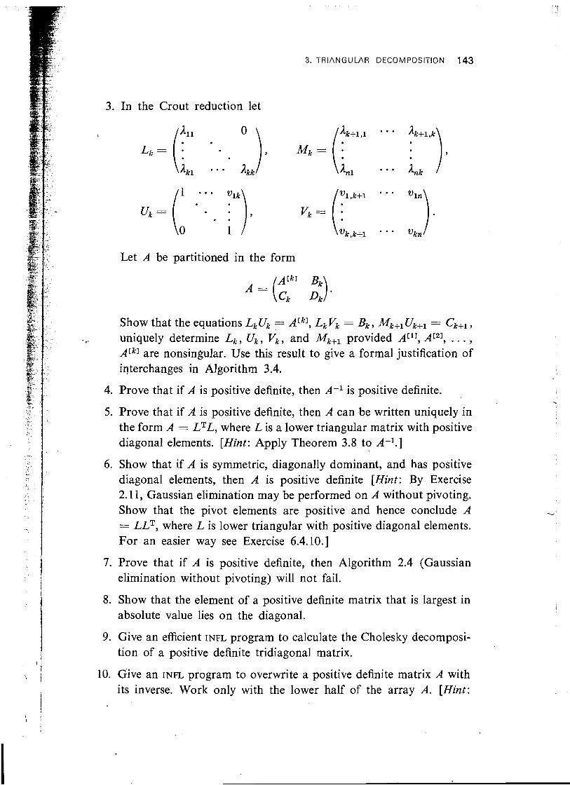
Show that the equations LkUk = ACkl, LkVk = Bk, Mk+lUk+l = Ckfl, uniquely determine Lk, Uk, Vk, and Mk+l provided A[ll, A[21, . . . , ALkl are nonsingular. Use this result to give a formal justification of interchanges in Algorithm 3.4.

4. Prove that if A is positive definite, then A-l is positive definite.

5. Prove that if A is positive definite, then A can be written uniquely in the form A = LTL, where L is a lower triangular matrix with positive diagonal elements. [Hint: Apply Theorem 3.8 to A-l.]

7. Prove that if A is positive definite, then Algorithm 2.4 (Gaussian elimination without pivoting) will not fail.

' -

I 8. Show that the element of a positive definite matrix that is largest in absolute value lies on the diagonal.

6. Show that if A is symmetric, diagonally dominant, and has positive diagonal elements, then A is positive definite [Hint: By Exercise 2.1 1, Gaussian elimination may be performed on A without pivoting. Show that the pivot elements are positive and hence conclude A

9. Give an efficient INFL program to calculate the Cholesky decomposition of a positive definite tridiagonal matrix.

= LLT, where L is lower triangular with positive diagonal elements. For an easier way see Exercise 6.4.10.1

10. Give an INFL program to overwrite a positive definite matrix A with its inverse. Work only with the lower half of the array A. [Hint:

I I


Use Algorithm 3.9 to compute L of the Cholesky decomposition. Then compute L-l and L-"L-I.]

11. Let A be positive definite. If one step of Gaussian elimination is performed on A, the result is a matrix of the form

Show that A' is positive definite.

12. Devise a variant of Algorithm 3.4 that, in the spirit of Exercise 2.20, avoids interchanges.


In view of the close connections between Gaussian elimination and methods of triangular decomposition, it is not surprising that many of the "new" methods that have appeared in the literature from time to time are simply rearrangements of Gaussian elimination. The term "LDU decomposition" is due to Turing (1948), who related it to Gaussian elimination. A complete discussion is given by Householder (1964). See also the book "Numerical Methods of Linear Algebra" by Faddeev and Faddeeva (1960, 1963), which although it is somewhat out of date, contains much other interesting material.

Programs implementing the Crout reduction have been published by Bowdler, Martin, Peters, and Wilkinson (1966, HACLA/I/7). The Cholesky decomposition has been implemented by Martin, Peters, and Wilkinson (1965, HACLAIIJl) for full positive definite matrices by Martin and Wilkinson (1965, HACLAJIJ4) for positive definite band matrices.

4. THE SOLUTION OF LINEAR SYSTEMS

In the introductory material to Section 2 we indicated how the method of Gaussian elimination could be used to solve the linear system

where A is of order n. In this section we shall describe in detail how the decompositions of Sections 2 and 3 can be used to solve (4.1). The essential feature of the resulting methods is that the reduction of A and the solution of (4.1) can be separated: once A has been reduced, the reduced form can be used to solve (4.1) for any number of right-hand sides 6.

4. THE SOLUTION OF LINEAR SYSTEMS 145

We consider first the use of Gaussian elimination with complete pivoting. Algorithm 2,10 defines elementary permutations Pi , Qi (i = 1, 2, . . . , n - l), and elementary lower triangular matrices Mi of index i such that

A, = Mn-lP,-lMn-2 . . MlPlAQlQ2 . . .

is upper triangular. Equation (4.1) can thus be written in the form

and the solution is given by

This suggests the following algorithm for solving (4.1).

ii9LGORITHM 4.1. Let P i , Q,, Mi (i = 1,2, . . . , n - 1) and A, be the matrices defined by Gaussian elimination with complete pivoting applied to A. Given the vector b, this algorithm computes the solution x of (4.1).

1) Yl = b

2) For k = l , 2 , . . . , n - 1

1) Yk+l=MkPk~k L 3) Solve the upper triangular system Anzn = y,

J

4) For k = n - 1 , n - 2 , . . . , 1

1) Zk = Q k ~ k + l

The only place where the algorithm can break down is in statement 3. However, if A is nonsingular, then so is A,, and the solution of A,zn = y, always exists. Hence, if A is nonsingular, Algorithm 4.1 can be carried to completion and yields the solution to (4.1).

It is instructive to consider the practical details of the implementation of Algorithm 4.1. In the first place, it is not necessary to store the y i and zi separately. Rather we can initially set x = b, and store each new vector in x as it is generated. Second, if Algorithm 2.10 is used to accomplish the Gaussian reduction, the matrices Pk , Q k , and Mk are given in terms of the numbers ek , yk, and pip. Since these matrices are of very simple form, it


would be wasteful of time and storage to generate them in full and perform the matrix-vector multiplications indicated by the algorithm. Instead we may compute one vector directly from its predecessor. For example, statement 2.1 can be accomplished by the sequence of computations

Finally, statement 3 can be accomplished by Algorithm 1.3. We sum up these considerations by rewriting Algorithm 4.1. In the

sequel, we shall describe the use of the other decompositions in the spirit of Algorithm 4.1, leaving the detailed recastings as exercises.

ALGORITHM 4.2. Given the output from Algorithm 2.10 and the n- vector b, this algorithm computes the solution of (4.1).

4) For k = n - 1 , n - 2 , . . . , 1

11) t k + + E Y k

If Algorithm 1.3 is used to accomplish step 3, Algorithm 4.2 requires about n2 multiplications for its execution. This should be compared with the n3/3 multiplications required to reduce A to triangular form. In other words, if we wish to solve a single linear system, the bulk of the work will be con- centrated in the initial reduction. Thereafter, additional systems with the same matrix but different right-hand sides can be solved at relatively little additional cost.

Turning now to the use of Gaussian elimination with partial pivoting, we note that the reduction with partial pivoting differs from the reduction with complete pivoting only in the absence of column interchanges. Hence, having performed Gaussian elimination with partial pivoting on A, we may obtain an algorithm for solving (4.1) by deleting step 4 from Algo- rithm 4.1.

4. THE SOLUTION OF LINEAR SYSTEMS 147

ALGORITHM 4.3. Let Pi and Mi (i = 1,2, . . . , n - l), and A , be the matrices obtained by applying Gaussian elimination with partial pivoting to A. Given the n-vector b, this algorithm computes the solution of (4.1).

2) For k = l ,2 , ..., n - 1

11) x-d'fkPkx

3) x.+ Ai lx

The Crout reduction of A with pivoting yields elementary permutations Pi ( i = 1,2, . . . , n - 1) such that

Pn-1Pn-2 . . PIA = LU, I

where L is lower triangular and U is unit upper triangular. Hence the solution of (4.1) is given by

This leads t o the following algorithm for solving (4.1).

ALGORITHM 4.4. Let LU be the Crout decomposition of P,-,Pn-, PIA, and let b be given. This algorithm computes the solution of (4.1).

2) For k = l , 2 , . . . , n - 1 1 1) x + P k x

3 ) x +- L-lx ,

I I

4) x + U-lx

The algorithm can be carried to completion if A is nonsingular and I requires about n2 multiplications. In statement 4 a minor saving can be

I effected by taking advantage of the fact that U is unit upper triangular. I I

When A is symmetric and positive definite, it has a Cholesky decomposi- I

tion in the form A = LLT, where L is lower triangular. Thus the solution I I of (4.1) is given by

I x = L-TL-lb

\ and we obtain the following algorithm.


ALGORITHM 4.5. Let LLT be the Cholesky decomposition of the positive definite matrix A, and let b be given. This algorithm computes the solution of (4.1).

1) zc = L-lb

Any of the above decompositions can be used to find the inverse of A, either by inverting and multiplying the matrices in the decomposition, or by solving the n linear equations

for the columns of tbe inverse. The details are left as exercises. Again it must be stressed that in applications the inverse of a matrix is seldom required (cf. Section 1).

EXERCISES

1. Devise an efficient algorithm for solving upper-Hessenberg systems (cf. Exercise 2.6).

2. Devise an efficient algorithm for solving tridiagonal systems (cf. Exercise 2.7).

3. Write an INFL program that takes the output of Algorithm 3.4 and .overwrites A with A-I by forming the product U-IL-I. Be careful of the interchanges.

4. Give detailed INFL code that uses the output of the algorithms of Exercises 2.19, 1.20, 2-21, and 3.12 to solve linear systems.

5. THE EFFECTS OF ROUNDING ERROR

In this section we shall discuss the effects of rounding errors on the algorithms described in this chapter. For example, we shall show that if the algorithms of Section 4 are used to compute a solution of the equation

the computed solution X satisfies

5. THE EFFECTS OF ROUNDING ERROR 149

and we shall give rigorous bounds on the sizes of the elements of H. If H can be shown to be small, then the algorithm is stable in the sense of Sec- tion 2.1.

Such an error analysis has two important limitations. In the first place, the error bounds are often far larger than the observed error. There are two reasons for this. First, in order to obtain reasonably simple error bounds one must use estimates that are obviously not sharp. Second, no rigorous upper bound on the error, however sharp, can satisfactorily account for the statistical nature of rounding error. It should not be concluded from this that the error analyses are useless. Even if the upper bound on H in (5.2) is an overestimate, it none the less guarantees the stability of the algorithm, provided it is reasonably small. In addition, an error analysis can suggest how to arrange the details of an algorithm for greater stability. For example, the bound on H in (5.2) contains factors that depend on the pivoting strategy used in the decomposition of A and thereby provides a rationale for choosing a pivoting strategy.

The second limitation is that a stability result such as (5.2) cannot insure the accuracy of the solution, unless the problem is well conditioned, for if the system (5.1) is ill conditioned, even a small random H will correspond to a large deviation in X. However, it may happen that the matrix H that results from rounding error has elements that are so correlated that X is accurate, even when (5.1) is ill conditioned. Our theorems will say nothing about this phenokenon, since they only bound the size of the elements of H. Such correlated errors actually occur in solving triangular systems, whose solutions are usually computed to high accuracy.

A rigorous rounding-error analysis proceeds by repeated applications of the rounding-error bounds of Section 2.1. Although the analyses are usually conceptually straightforward, they are fussy in detail. For this reason we shall only state the results of the rounding-error analyses in this section (however, some of the analyses are given in Appendix 3). We shall assume that all calculations have been performed in t-digit floating-point arithmetic satisfying the bounds of Section 2.1. We further assume that underflow and overflow have not occured in the calculation. Finally, we assume that the order of the problem considered, say n, is so restricted that np . < . I . This restriction, which in practice is always satisfied, is necessary to obtain bounds in a reasonably simple form (cf. Exercises 2.1.4 and 2.1.5).

We turn first to the solution of triangular systems by Algorithm 1.3.

150 3. 'THE DIRECT SOLUTlON @ F LINEAR SYSTEMS

THEOREM 5.1. Let T E: Rnxn and b E Rn. Let X denote the computed solution of the equation Tx = b obtained from Algorithm 1.3. Then X satisfies the equation

(T + E)X = b,

where

I EG 1 5 (n + 1)n 1 t~ 1 (i, j = 1,2, . . . , n). (5.3)

Here n is a constant o f order unity that depends on the details of the arithmetic.

This theorem is in many respects quite satisfactory. It says that the computed solution is an exact solution of a problem in which T has been perturbed slightly. In fact the elements of T + E differ from the corresponding elements of T by small relative errors. For moderate n, these relative errors are comparable to the errors made in rounding T itself, and if the elements of Tare themselves computed, the errors E~~ may be considerably smaller than .the uncertainty in T. If inner products are accumulated in double precision, the factor n may be dropped from (5.3), so that the error matrix E is quite comparable with the error made in rounding T.

None the less, the above results illustrate the limitations mentioned at the first of this sectjon. In the first place, the details of the analysis show that

I EG I 5 ( j - i + 2)n I sij 1 lo-',

which may be considerably smaller than (5.3). More important, though, is the fact that the solutions of triangular systems are usually computed to high accuracy. This fact, which is not a consequence of Theorem 5.1, cannot be proved in general, for counter examples exist. However, it is true of many special kinds of triangular matrices and the phenomenon has been observed in many others. The practical consequences of this fact cannot be over- emphasized.

The question of whether Algorithm 1.4 for inverting an upper triangular matrix is stable is open. Since each column si of the inverse was formed by solving the system Tsi = ei, it follows from Theorem 5.1 that si is the ith column of the inverse of a slightly perturbed matrix T + Ei . However, since the perturbation is different for each i, it does not follow that S = (s,, s,, . . . , s,) is the inverse of some perturbed matrix T + E or even that S is near .the inverse of such a matrix.


None the less, in practice the computed inverses of triangular matrices are usually found to be quite accurate. This is to be expected, since the inverse is obtained by solving a set of triangular systems, and we have already observed that the solutions of triangular systems are usually computed with high accuracy. Moreover, it can be shown that for some special classes of matrices the computed inverse must be accurate, although nothing can be proved in general.

We shall now consider the error analyses of Gaussian elimination and the algorithms for triangular decomposition. We have already seen that the strategy for selecting the pivots in these algorithms can have a marked effect on their numerical properties, and we should expect the error analysis to reflect the pivoting strategy. It turns out that the choice of pivots affects the outcome by limiting the growth of elements computed in the course of the reduction.

This point is most clearly illustrated by Gaussian elimination. By Theo- ' rem 2.9 we may assume that any interchanges required by the pivoting

Kg.:. ! strategy have already been performed. Thus let the algorithm for Gaus-

;$..! .*5 ', ..

sian elimination without pivoting be performed in floating-point arith- -<e. , 1 . i i . ,

,

.z: . ,;.;, metic on the matrix A = A, yielding matrices MI , M, , . . . , M,-, , and .:: .. . . 1; . . . . . . . 2.: ; A,, A,, . . . , A,. Let .g . ,

and

Thus y, the ratio of the largest element of A,, A,, . . . , A, to the largest element of A,, is a measure of the growth of the matrices generated by the algorithm. With these definitions, we have the following result.

THEOREM 5.2. The matrices MI , M,, . . . , M,-, , A, computed by Al- gorithm 2.4 satisfy

MT' Mgl . M;l,A, = A + E, (5.4)

where

\ for some constant n of order unity that is independent of A.


By the theorem, the computed triangular decomposition obtained from Gaussian elimination is the exact triangular decomposition of a perturbed matrix. The perturbation will be small compared to /I, (that is, compared to the largest element of A,) provided the growth factor y is small. Thus it is important to establish bounds on the growth of the elements in the course of the reduction. For partial and complete pivoting upper bounds can be given for y that do not depend on A. The bound for complete pivoting is

This bound increases rather slowly with n, and moreover the proof that establishes it shows that it cannot be attained. In fact, no matrix with real elements is known for which y is greater than n. Thus Gaussian elimination with complete pivoting is a stable algorithm.

The bound for partial pivoting is

This is a rather fast growing function, and its use in the bound (5.5) suggests that the order of those matrices that can be safely decomposed by Gaussian elimination with partial pivoting is severely limited. For example, on a four-digit machine, if A, is of order 12, the elements E may be of the same size as the elements of A. Unfortunately matrices are known for which this bound on y is attained, so that we cannot assert that Gaussian elimination with partial pivoting is unconditionally stable.

In practice, however, the bound (5.6) is seldom attained. Usually the elements of the reduced matrices A,, A,, . . . , A . remain of the same order of magnitude or even show a progressive decrease in size. Moreover, for many commonly occuring kinds of matrices, such as Hessenberg matrices, the growth is much more restricted. Thus in practice Gaussian elimination with partial pivoting must be considered a stable algorithm.

The error analysis of the Crout reduction yields similar results. The computed L and U satisfy

where the elements of E satisfy (5.5). The growth factor y in the bounds for the Crout reduction is the same as the growth factor for Gaussian elimination. We have already noted that with partial pivoting y can increase swiftly with the order'of the matrix. Since partial pivoting is the only

5. T H E EFFECTS OF ROUNDING ERROR 153

convenient strategy for the Crout reduction, we cannot claim that this reduction is stable in general. However, .the observation that large growth factors are almost never encouiltered applies here, and for practical purposes the Crout reduction can be considered a stable algorithm.

We have mentioned earlier that an important reason for preferring the Crout reduction to Gaussian elimination is that the Crout reduction permits the accumulation of inner products in double precision. As far as the rounding-error analysis is concerned, the effect of this is to remove .the factor n from the bound (5.5). Thus if y is also of order unity, the elements of the error matrix E are of the same size as the errors made in rounding A, and in many ca3es they will be considerably smaller. This is about as much as'can be expected in the way of stability.

The error analysis of the Cholesky algorithm for positive definite matrices differs from the others in that there is no growth factor (this is also true of Gaussian elimination and Crout reduction applied to positive definite matrices; see Exercise 5.2). In fact, we can prove that the algorithm computes a lower triangular matrix L satisfying

where the elements of E satisfy (5.5) with y = 1. When inner products are accumulated in double precision, the factor n may be removed from the bounds. Thus the Cholesky algorithm for positive definite matrices is unconditionally stable.

It should be stressed that the results quoted here for Gaussian elimination and the algorithms for triangular decomposition are the final, simplified results of rather detailed error analyses. An examination of the details of the analyses shows that the bounds on the elements of E are, in many frequently occurring cases, severe overestimates. Nonetheless, the above results indicate the major features that determine the stability of the algorithms.

For example, these bounds have something to say about the delicate question of choosing between Gaussian elimination with complete pivoting, Gaussian elimination with partial pivoting, and the Crout reduction with partial pivoting. When inner products cannot be accumulated in double precision the Crout reduction and Gaussian elimination have the same numerical properties. When inner products can be accumulated in double precision, the Crout reduction is superior. Thus there seems to be little reason for using Gaussian elimination with partial pivoting. This conclusion


is reinforced by the fact that a Crout reduction program that does not accumulate inner products in double precision can be converted into one that does with very little trouble.

The choice is then between Gaussian elimination with complete pivoting and the Crout reduction. A reason customarily advanced against the former is that searching the entire matrix for the largest element is inordinately time consuming. This will generally be true if the algorithm is coded in one of the standard languages such as FORTRAN. However, if the algorithm is coded in machine language, the search can be performed as the elements are computed, usually at little additional cost. Since the stability of Gaussian elimination with complete pivoting is guaranteed, a person of conservative temperament who is willing to put up with a machine dependent subroutine might prefer it over the Crout reduction. On the other hand, practically speaking the Crout reduction has the same stability as Gaussian eliminatioil with complete pivoting and can be coded efficiently in, say, FORTRAN. If inner products can be accumulated in double precision, the Crout reduction is superior, except in the unlikely cases where there is a significant growth in the elements.

Bounds for the solution of the linear system Ax = b may be obtained by combining Theorem 5.1 and 5.2. For definiteness we shall suppose that the matrix A has been decomposed by Gaussian elimination with partial pivoting into the product

The elements of L are the multipliers pij of Algorithm 2.4, which are less than unity in magnitude. Hence

The elements of U are taken from the matrices A,, A,, . . . , A, of the reduction and hence satisfy

where B, is the magnitude of the largest element of A, and y is the growth factor. Finally from Theorem 5.2 we know that

where the elements of E satisfy (5.5).


Now suppose that Algorithm 4.3 is used to solve the system A x = b. Statement 2 of the algorithm is numerically equivalent to solving the lower triangular system

Ly = b, (5.8)

while statement 3 amounts to solving the upper triangular system

We have observed that triangular systems are usually solved with high accuracy. Hence it is not surprising that the computed solution Z is often very near the true solution X of the system

In other words, the computed solution X of a system of linear equations is often near a solution X of (5.9), where the error matrix E is independent of the right-hand side b. However, this is not a rigorous result and counter examples can be constructed. The following theorem shows that if we drop the requirement that the error matrix be independent of the right-hand side, we can obtain a rigorous stability result.

THEOREM 5.3. Let 3 denote the solution of the system Ax = b computed by Algorithm 4.3. Then X satisfies

where

1 vij / 5 (nn + 2n2e + n3~210-t)y~110-t, (5.11)

with n and Q constants of order unity.

PROOF. By Theorem 5.1, the computed solution 7 of (5.8) satisfies

where

< ne 1 A, I lo-t 5 nelO-t I 4ij I -

with Q a constant of order unity. The last inequality follows from the fact that partial pivoting insures that 1 Aij 1 5 1. In statement 3 of Algorithm

156 3. THE DIRECT SOLUTION OF ILINEAR SYSTEMS

4.3 we solve the system Ux = 7, yielding a computed solution 2 that satisfies

(U + G)Z = 7 (5.13)

where

I yij I I ne I vij 1 _( ne/l,ylO-t.

Combining (5.7), (5.12), and (5.13), we find that x' satisfies (5.10) where

Now the largest element of the product of two matrices of order n is bounded by n times the product of the largest elements of each matrix. Hence, using the bounds for the elements of E, F, G, L, and U, we obtain (5.1 1). .

The error matrix H of course depends on the vector b, since the matrices " F and G do. The bound (5.11) on its elements depends critically on the

growth factor y. If y is of order unity and n is not unreasonably large, the elements of H will be not too much larger than the errors made in rounding A ; often they will be a good deal smaller. The term containing n2 comes from the errors made in solving triangular systems. Since, as we have noted, these errors are often negligible, the true error may be more accurately reflected by the term nn.

Analogs of Theorem 5.3 hold for the Crout and Cholesky algorithms. If inner products are accumulated in double precision throughout the calculations, the first factor in (5.11) may be replaced by

In many cases the term 2 n ~ , which accounts for the errors introduced by solving the triangular systems, may be omitted, so that the bound becomes effectively independent of the size of the matrix.

Since no general theorems on the computed inverses of triangular equations have been established, it is not surprising that little can be said about the computed inverses of general matrices. Suppose, for example, that the columns of the inverse X, are computed as the solutions of the systems Axi = ei (i = 1,2, . . . , n). Then from Theorem 5.3 we know that each computed column Xi satisfies (A + Hi)Xi = ei; however, the error matrices Hi may be different for each column, and we cannot conclude that there is a single small matrix H such that (A + H)X = I.


None the less, it follows from the remarks preceding Theorem 5.3 that each Xi will often be near the solution Xi of the equation ( A + E)Ri = ei, where E is the error matrix from the LU decomposition of A. Since E is independent of the right-hand side ei, it follows that is near an inverse of A + E. This means that in many cases the error in the computed inverse of A will be almost entirely due to the errors made in computing the LU decomposition of A.

All of the rigorous results established in this section concern the stability of algorithms. The only results on the accuracy of computed solutions were in the form of informal observations. In Section 5.4 we will apply the theory of norms to obtain rigorous bounds on the errors in computed solutions.

We conclude this section with a word of caution. The factor PI, which appears in the error bound of Theorem 5.2, serves the purpose of a normalizing factor. In effect the bound says that the error will be small compared to PI , that is compared to the largest element of A. If all the elements of A are of about the same size, then this is a perfectly satisfactory result. On the other hand, if there is a wide disparity in the sizes of the elements of A, there is a danger that the smaller elements will be overwhelmed by the errors. If these small elements are critical to the reduction, the results will be inaccurate.

For example, consider the matrix

which was obtained from the matrix of Example 2.8 by multiplying its first row by 3000. If Gaussian elimination with partial pivoting is performed in four-digit arithmetic on A, the (I, 1)-element is accepted as the first pivot, and the calculation proceeds exactly as in Example 2.8 with a disasterous cancellation occuring in the computation of the (3, 3)-element of the reduced matrix. Our error analysis guarantees that the computed decomposition is the exact decomposition of A + E, where the elements of E are of the order P1 . however, this is small consolation, for P1 = 9000 and the elements of E can be, and are, as large as unity.

Since the disparity in the sizes of the elements of A is responsible for the problem, it is natural to attempt to scale the rows and columns of A so that the matrix is balanced. A frequently suggested method is to scale A so that the largest element in each row and column lies between, say, 1 and 10.

158 3. THE DIRECT SOLUTION OF I-IP.IEAR SYSTEMS

For example, the original matrix of Example 2.8, which can be reduced safely by Gaussian elimination with partial pivoting, satisfies this criterion. However, the matrix

obtained from (5.14) by dividing the second column by 6000 and the third column by 9000 also satisfies the criterion. It is easily verified that, in four- digit arithmetic, even complete pivoting will not yield an accurate reduction. The error matrix associated with the reduction has elements of order but this is no help since four of the elements of A are also of order

The difficulties involved in scaling can be overstressed. For many problems the criterion suggested above is quite satisfactory and for many others the correct scaling is perfectly evident. However, the above example shows that pat scaling strategies are suspect. In spite of intensive theoretical investigation, there is no satisfactory algorithm for scaling a general matrix.

EXERCISES

1. Compute the last column of the inverse of

in four-digit arithmetic. Interpret your results.

2. Show that if Gaussian elimination is applied to a positive definite matrix, then the growth factor y of Theorem 5.2 is equal to unity. [Hint: Show that the diagonal elements must decrease and then apply Exercises 3.8 and 3.1 1.1

3. Show that if A is upper Hessenberg of order n, then the growth factor y for Gaussian elimination with partial pivoting is bounded by n.

4. Show that if A is tridiagonal, then the growth factor y for Gaussian elimination with partial pivoting is bounded by two.

5. Show that if is diagonally dominant, then the growth factor y for Gaussian elimination with partial pivoting is bounded by two.

EXERCISES 159


All the material in this section is contained in works by Wilkinson (1961 ; 1963; AEP, Chapter IV). The 1961 paper contains a wealth of detail: in particular, a derivation of bounds for the growth factors for matrices of special form and a discussion of the high accuracy of the computed solutions of triangular systems.

The conjecture that the growth factor for complete pivoting is bounded by the order of the matrix has neither been proved nor disproved. Cryer (1968) proves the conjecture for matrices of order four and surveys other attempts.

For more on the problem of scaling or equilibration, as it is sometimes called, see the works by Bauer (1963), Forsythe and Strauss (1955), and Wilkinson (1961; AEP, Chapter IV).

NORMS, LIMITS, AND CONDITION NUMBERS CHAPTER 4

With few exceptions we have, in the first three chapters of this book, con- fined ourselves to the algebraic properties of vectors and matrices; that is we have developed those areas that could be described in terms of algebraic operations without requiring the notion of limit. In this chapter we shall introduce the ideas of norm and limit and apply them to the problems of assessing and improving the accuracy of approximate solutions of linear systems.

A vector norm on Rn is a function from Rn into the nonnegative real numbers whose value in some sense measures the size of a vector in Rn. Examples of norms are the absolute value in R and the Euclidean length of a vector in R? The idea of norm is closely related to the idea of limit, as is suggested by the equivalence

lim E~ = f e lim ( f - Ek I = O. k + m k + w

In Section 1 we shall introduce the idea of a vector norm on Rn and explore its relation to limits in Rn. In Section 2 we shall extend the concept of r,crrm to matrices. In Section 3.5, we discussed the effects of rounding

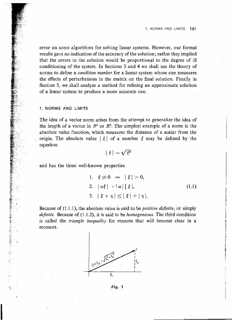
1. NORMS AND LIMITS 161

error on some algorithms for solving linear systems. However, our formal results gave no indication of the accuracy of the solution; rather they implied that the errors in the solution would be proportional to the degree of ill conditioning of the system. In Sections 3 and 4 we shall use the theory of norms to define a condition number for a linear system whose size measures the effects of perturbations in the matrix on the final solution. Finally in Section 5, we shall analyze a method for refining an approximate solution of a linear system to produce a more accurate one.

1. NORMS AND LIMITS

The idea of a vector norm arises from the attempt to generalize the idea of the length of a vector in R1 or R2. The simplest example of a norm is the absolute value function, which measures the distance of a scalar from the origin. The absolute value I f ( of a number 5 may be defined by the equation

I e l =@

and has the three well-known properties

Because of (1.1. I), the absolute value is said to be positive definite, or simply de$nite. Because of (1.1.2), it is said to be homogeneous. The third condition is called the triangle inequality for reasons that will become clear in a moment.

Fig. 1

162 4. NORMS, LIMITS, AND CONDITION NUMBERS

A less trivial example of a norm is the Euclidean length of a vector in R2. For any x E R2 it is denoted by ) [ x 1 1 , and defined by

By the Pythagorean theorem, 1 1 x [ I 2 is the distance from x to the origin (Fig. 1).

The Euclidean norm 1 1 . ) I 2 satisfies three conditions that correspond to .the properties (1.1) satisfied by the absolute value. Specifically,

The first two conditions are clear from the definition of 1 ) . 1 1 , . The third " condition may be interpreted geometrically as saying that the length of a

side of a triangle is not greater than the sum of the lengths of the other two sides, whence the name triangle inequality (Fig. 2).

Fig. 2

One natural way of extending these ideas to Rn is to generaIize formula (1.2) in the obvious way to obtain a Euclidean length of a vector in Rn. However, this is somewhat restrictive, for there are many other functions that measure the size of a vector. For example, the number v(x) defined for x E R2 by

4 x 1 = max(l 1 , 1 R 1 ) (1.3)

is also a reasonable measure of the size of x and is computationally more convenient than (1.2). It turns out that in many applications, all that is required of a measure of size is that it be definite, homogeneous, and satisfy the triangle inequality. This motivates the following definition.


DE FlNlTlON 1 .l. A vector norm (or simply a norm) on Rn is a function v : Rn + R that satisfies the following conditions:

The absolute value function is a norm on R1, and the function ) I . 11, defined by (1.2) is a norm on R2. The function v defined by (1.3) is also a norm on R2.

The definition of norm has some elementary consequences. By property 1.1.1, the function v is positive except at the zero vector. By property 1.1.2,

i 1 An important inequality is the following.

,

I

which in terms of the Euclidean norm says that the length of a side of a triangle is not less than the difference of the lengths of the other two sides (Fig. 3). To establish it, note that

so that the norm of the zero vector is zero. Also from 1.1.2, it follows that

v(-x) = v(-1 . x) = I -1 ( v(x) = v(x).

Hence

Fig. 3


If x and y are interchanged in (1.5), we obtain

v(y) - v(x) ( v(y - x) = v(x - y).

Inequalities (1.5) and (1.6) together imply (1.4).

If y is replaced by -y in (1.4), there results the related inequality

We turn now to the construction of specific vector norms. We begin with three norms on Rn that are frequently used in analyzing matrix processes. They are the I-, 2-, and oo-norms defined by

and 1 1 X I ] , = max(1 ti( : i = 1,2, . . . , n ) .

The 2-norm is the natural generalization of the Euclidean length of a 2- or 3-vector and is also called the Euclidean norm. The oo-norm is sometimes called the maximum norm (max-norm) or the Chebyshev norm.

All three functions [ I . (I,, I ( (I2, and ( 1 . (1, are obviously definite and homogeneous. Moreover, it is easy to show that 11 11, and 1 ) 11, satisfy the triangle inequality. For example,

To establish the triangle inequality for the 2-norm we require an inequality which is important in its own right. It is the well-known Cauchy inequality (which, incidentally, is also associated with the names Schwarz and Bunya- kovski).


THEOREM 1.2. For all x, y E Rn,

I xTy I I I I x 112 I I Y 1/29 (1.7)

with equality if and only if x and y are linearly dependent.

PROOF. If either x or y is zero, the theorem is trivially true. Hence suppose that both x and y are nonzero. Then ( 1 x 1 1 , and 1 1 y ( 1 , are both

jf nonzero. Let x' = x / J ( x ( 1 , and y' = y/ll y l l z . Then ) I x' 11, = ) I y' 1 1 , = 1,

$ and the inequality (1.7) is equivalent to the inequality U' * - @" I x IT y 1 1 5 1 .

Now suppose xtTy' 2 0. Then

0 5 1 ) x' - y' 1 ) ; = (x' - Y ' ) ~ ( x ' - y ' )

' T ' 'T ' = xtTy' + y y - 2x y T$ 'T ' T = II x' 1 1 ; + I I Y' Ilt - 2x Y &: ' T '

$% 8 = 2 - 2 x y . (1.8) 47' g, A Hence xtTy' 5 1. If xfTy' < 0, the inequality -xtTy' 5 1 follows similarly,

with x' + y' replacing x' - y' in (1.8). ' I Now suppose I xTy 1 = I ( x 1 1 , J l y 1 1 , with say xTy 2 0. This can only

happen when the inequality in (1.8) is an equality. Hence 1 ) x' - y' ( 1 , = 0, and x' = y'. This implies that

x = I / x 112

I 1 Y 112 Y

and hence that x and y are linearly dependent. The case xTy < 0 is treated similarly.

Finally, suppose that x and y are linearly dependent. Since y # 0, x = ay for some scalar a. Then ( 1 x ( 1 , = 1 a ( ( 1 y I / , , and

I xTyI = I a I y T y = I a I I lY 112 IIY I12 = IIxII2 IIY 112. . The above proof makes heavy use of the identity 1 1 x 1 1 ; = xTx. This

characterization is also used in establishing that 1 ) ( 1 , is a norm.

-.. THEOREM 1.3. The function 1 1 I), satisfies the triangle inequality.

166 4. NORMS. LIMITS. AND CONDITION NUMBERS

PROOF. The proof is purely computational.

I I x + Y III = ( x + yIT(x + Y )

= xTx + 2xTy + yTy

< I l x 11; + 2 1 1 x 112 ll Y 112 + t i Y 11: = C l l x 112 + l l Y 11212,

where the inequality follows from the Cauchy inequality.

We have used the same symbol [I . I ( , to denote the 2-norm on R1, R2, R3, . . . . While this is not a serious abuse of notation, it can be avoided by introducing some terminology which will prove useful later in connection with matrix norms.

DEFINITION 1.4. Let v : U,"==, P-t R. Then v is a family of vector norms if for each n = 1,2, 3, . . . the restriction of v to Rn is a norm.

Thus each of the functions 1) )I1, 11 I ) , , 1 1 . 11, is a family of vector norms. Incidentally, these norms are special cases of the Holder norms or p-norms defined by

(11 x 11, is lim,,, ( 1 x 11, .) A proof that these are indeed norms will be found in the exercises.

A useful technique for constructing new norms from old is contained in the following theorem.

I

1

! \

THEOREM 1.5. Let v be a norm on Rm and A E Wmxn have linearly 1 independent columns. Then the function ,u : Rn -+ R defined by

1 i

is a norm on Rn.

1 i PROOF. Because A has linearly independent columns and v is a norm, I


Hence p is definite. Since

p is homogeneous. Finally,

so that p satisfies the triangle inequality. . Theorem 1.5 may be applied to give an important class of norms.

THEOREM 1.6. Let A E Rnxn be positive definite. Then the function Y : Rn -+ IR defined by

Y ( x ) = @Zi " is a norm on Rn.

PROOF. By Theorem 3.3.8, A can be written in the form A = LLT, . where L is a nonsingular lower triangular matrix. Then

Hence by Theorem 1.5, v is a norm. . Note that when A = I, the function Y of Theorem 1.6 reduces to the

2-norm. The notions of norm and limit are closely connected, and in more abstract

settings it is often convenient to define the notion of limit in terms of a norm. However, in Rn there is a very natural definition of limit in terms of limits of real numbers. We shall start with this definition and explore its connection with vector norms later (Theorem 1.12). We begin with a review of the properties of limits of real numbers.

We shall denote a sequence a, , a,, a,, . . . by (ak). The E - N definition of the limit of a sequence of real numbers may be found in almost any calculus text. For our purposes, we need only the elementary properties of the limit. Specifically, the sequence (ak) can have at most one limit. If (ak) has the limit a , we write

a = lim ak, k-z cc

168 4. NORMS, LlMITS, AND CONDITION NUMBERS

or, when it will cause no confusion,

a = lirn ak.

If a = lirn ak and P = lirn P k , then

and

lirn akPk = aP.

Moreover, if a # 0, then, for all sufficiently large k, ak # 0 and

Finally we have the characterization

lim ak = a o lim I a - ak ( = 0. (1.10)

In discussing limits of vectors, we shall need to refer to the components of a sequence of vectors. To do this we shall adopt .the following convention. If ( x k ) is a sequence of n-vectors, we shall denote the ith component of xk by f j k ) . We have already used this convention in Section 3.2 in connection with the matrices Ak generated by Gaussian elimination.

In Rn it is natural to say that a sequence of vectors converges to a limit of each if its components converges to a limit. For example, in R2 we should say that the sequence of vectors

is converging to the vector (2, On the other hand, we should say that the sequence

has no limit, since the second component never settles down. This suggests the following definition.


DEFINITION 1.7. Let (x,) be a sequence of n-vectors and let x E Rn. Then x is a limit of the sequence (xk) (written x = limk+, xk) if

lim tik' = ti (i = 1, 2, . . . , n). k- tw

Since the limit of a sequence of real numbers is unique, Definition 1.7 implies that the limit of a sequence of vectors must be unique. Moreover, the vector limit has some of the algebraic properties of the scalar limit, as the following theorem shows.

THEOREM 1.8. Let the sequences (ak), (bk), and (Ak) have limits a, b, and A. Then

lim(ak & bk) = a & b (1.1 1)

and lim Akak = Aa. (1.12)

PROOF. We prove (1.1 I), leaving (1.12) as an exercise. By Definition 1.7, we know that lim aik) = ai and lim pik) = pi, and we must show that

lim (a:*' f pik)) = ai f pi (i = 1, 2, . . . , n). k-tw

However, for each i, this is simply (1.9). . The relation between limits and norms is suggested by the equivalence

(1 .lo). Namely, if v is a norm on Rn and (xk) is a sequence of n-vectors, then lim xk = x if and only if lim v(=c - x,) = 0. However, the proof of this fact requires a fairly deep result on the equivalence of norms. To illustrate its statement, consider the following scalar inequalities:

n max{l tiI : i = l , 2 , . . ., n ) 5 C I f i l <nmax{l tiI : i = 1, 2, . .., n ) .

i-1

In terms of norms, the inequalities state that in P

Thus whenever 1 ) . 1 1 , appears in an expression as an upper bound, we may replace it by n ( 1 (I,. Whenever I / . 1 1 , appears as a lower bound we may replace it with 1 . 1 ) . 11,. In other words, by multiplying the m-norm by

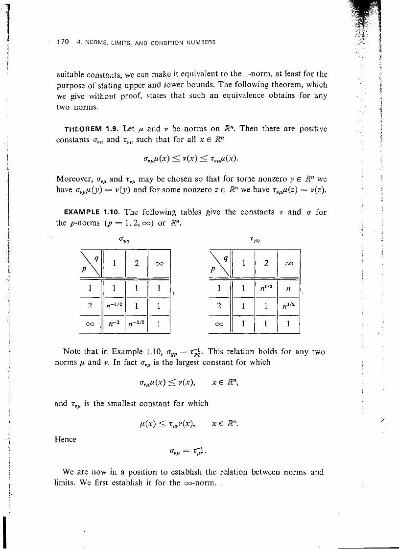
suitable constants, we can make it equivalent to the 1-norm, at least for the purpose of stating upper and lower bounds. The following theorem, which we give without proof, states that such an equivalence obtains for any two norms.

THEOREM 1.9. Let p and v be norms on Rn. Then there are positive I constants a,, and z,, such that for all x E Rn

Moreover, cr,, and z,, may be chosen so that for some nonzero y E Rn we have a,,p(y) = v ( y ) and for some nonzero z E Rn we have z,,p(z) = ~ ( z ) .

EXAMPLE 1 .lo. The following tables give the constants z and a for the p-norms (p = 1,2, 00) or Rn.

I I Note that in Example 1.10, a,, = z;;,1. This relation holds for any two I norms p and v. In fact cr,, is the largest constant for which !

I I and z,, is the smallest constant for which

!

t Hence

\ a,, = ti:.

We are now in a position to establish the relation between norms and limits. We first establish it for the oo-norm.

EXERCISES 171

LEMMA 1.1 1. Let (x,) be a sequence of n-vectors and x E Rn. Then

lirn xk = x a lim 1 1 x - xk = 0.

PROOF. From Definition 1.7 and the equivalence (1.10) we have the following equivalences.

limxk = x a lim tlk) = ti (i= 1,2, . . . , n)

a lim 1 ti - t!k) 1 = 0 ( i = 1,2, . . . , n)

a lirn max(1 ti - [!k)) : i = 1,2, . . . , n ) = 0

a lirn ) I x - xk (1, = 0. . THEOREM 1.12. Let v be a norm on Rn and x ,x , ,x , ,x , , . . . €Rn.

Then lim xk = x e lim v(x - xk) = 0. (1.13) k-tw k-tw

PROOF. If lim xk = x, by Lemma 1.11 we have lim ) ( x - xk (1, = 0. However, by Theorem 1.10, v(x - xk) 5 z,, ( 1 x - xk IJw. Hence lim v(x - xk) = 0. Conversely, let lim v(x - xk) = 0. Then by Theorem 1.10, 1 1 x - xk 11, ( Z,V(X - xk), and hence lirn 1 1 x - xk (1, = 0. By Lemma 1.1 1, we have lirn xk = x. .

The importance of Theorem 1.12 is that it allows us to use the right- hand side of (1.13) as an alternate definition of limit. Since the norm v is completely arbitrary, it may be chosen, say, to make it easy to show that lim V(X - xk) = 0. However it is chosen, though, we are assured that if lirn V(X - xk) = 0, then lirn xk = x in the sense of Definition 1.7.

EXERCISES

1. Show that if v : R1 -+ R is a norm, then v[(t)] = A [ t 1 , for some A > 0.

2. Show thai the function v defined by Equation (1.3) is a vector norm.

3. Prove the polarization identity

172 4. NORMS. LIMITS, A N D COIVDlTlON NUMBERS

4. Show that 1 1 - ( I , satisfies the triangle inequality.

5. Show by example that the condition that A have linearly independent columns cannot be removed from Theorem 1.5.

6. Let a,, a,, . . . , a, be positive. Show that the function v : Rn -+ R defined by v(x) = (Cr=, aiEi2)l/' is a norm.

7. Find linearly independent vectors x and y such that ( 1 x + y 1 1 , = I 1 x llm + l l Y llm-

8. Show that ( 1 x + y I ) , = 11 x ( 1 , + J j y ( 1 , if and only if x and y are linearly dependent and xTy > 0.

9. Let v be a norm on Rn and let 9, = ( x : V ( X ) ( 1 ). Prove that 9, satisfies .the following conditions.

1. There is an E > 0 such that ( x : 1 1 x 1 1 , ( E ) c 9,. 2. (Convexity) If x , y E 9, and a, P are nonnegative scalars with

a + ,8 = 1 , then ax + ,8y E 9,. 3. (Equilibration) If x E 9, and ( a I 5 1 , then a x E 9,.

The set 9, is called the "unit v-ball."

10. Describe the unit I - , 2-, and co-balls in R2; in R3.

1 1 . Establish the bounds of Example 1.10. For each a arid z give the vectors y and z promised in Theorem 1.9.

12. Prove that ( 1 x 11, = limp+, ( 1 x 11,.

13. Show that if p, q > 1 with p-I + q-I = 1 , then I q3 I ( I a l p i p

+ 1 P Iq/q, for all scalars a and p. [Hint: Show that the function # ( z ) = zP/p + z-q/q satisfies # ( z ) > 1 for all positive z. Let z = 1 a 1 l / q 1 p 1 - l /p . ]

14. (Holder inequality) Prove that if p, q > I with p-' + q-l = 1 and X,Y E R", then I xTy ( 5 / I x 1 1 , l l Y I . [Hint: Asslm-le I 1 x \ I p = I 1 Y l l q - 1 , and apply Exercise 3 to I Ei 1 / qi 1 . Then sum.]

15. (Minko~rlski inequality) Let x , y E Rn. Show that for 1 < p < ca that I l x + Y l l , 5 I 1 x 1 1 , + l l Y 1 1 , . [Hint: I 1 + Y llp 5 ( 1 1 x llp

+ ( 1 y Ilp)(CT=l 1 & + qi I q ( p - l ) ) l / q , where p-l + q-l = 1 . ]

2. MATRIX NORMS 173

2. MATRIX NORMS

In this section we shall consider the problem of extending the idea of a vector norm to matrices. At first glance this does not seem to be a very difficult problem. We have seen (page 32) that the set of matrices Rmxn is a vector space which is essentially identical with Rmn. Consequently any vector norm on Rmn induces a definite, homogeneous function on Rmxn that satisfies the triangle inequality, and it is natural to call such a function a matrix norm. For example, the 2-norm on Rmn induces the Frobenius norm ( 1 llF on Rmxn defined by

The same proof that 1 1 . I(, is a vector norm shows that ( 1 . ) I F : Rmxn -+ R is a definite, homogeneous function that satisfies the triangle inequality

We shall adopt this general definition of matrix norm. However, most matrix norms defined in this way are not very useful. The reason is that this definition of matrix norm gives no relation between the norms of two matrices and the norm of their product. Consequently we shall restrict our attention to matrix norms satisfying a consistency condition, which for the Frobenius norm reads

1 1 AB I ~ F 5 1 1 A /IF 1 1 B (IF. (2.2)

We begin our development with the general definition of matrix norm.

DEFINITION 2.1. A function v : Rmxn + R is a matrix norm on Rmxn if

( I ) A # 0 v(A) > 0, A E RmXn,

(2) v(aA) = ( a ( v(A), A E Rmxn, a E R,

This definition has some immediate consequences. Since a matrix norm on RmXn is essentially a vector norm on Rmn, it follows that a matrix norm enjoys all the properties of a vector norm. In particular, any two matrix norms on Rmxn are equivalent in the sense of Theorem 1.9. This means

I that if we define convergence in Rmxn, in analogy with Definition 1.7, as

174 4. NORMS. LIMITS, AND CONDITION NUMBERS

elementwise convergence, then lim A,, - A if and only if lim v ( A - Ak) = 0 for any matrix norm v. We shall return to the subject of limits of matrices at the end of this section.

Since we have agreed to identify n x 1 matrices with n-vectors, any matrix norm on Rnxl is also a vector norm on Rn, and conversely. As with vector norms, we may speak of families of matrix norms.

DEFINITION 2.2. The function v : Rmxn -t R is a family of matrix norms if for each m, n 2 1 the restriction of v to Rmxn is a matrix norm.

It follows from this definition and the preceding comments that if v is a family of matrix norms, then the restriction of v to U,"=, WnX1 is a family of vector norms.

EXAMPLE 2.3. The Frobenius norms defined for any A E Rmxn by (2.1) form a family of matrix norms. The restriction of ( 1 / I F to Uz=, Rnxl is the family of vector 2-norms; that is ( 1 x = I( x 11, for all vectors x.

The Frobenius norm is a natural generalization of the Euclidean vector norm. Since it is relatively easy to compute and satisfies the inequality (2.2), it is used rather frequently in matrix computations. However, all matrix norms satisfying Definition 2.1 need not satisfy an inequality such as (2.2). For example, a natural generalization of the oo-norm is the function v defined for A E Rmxn b Y

It is easily verified that v is a matrix norm in the sense of Definition 2.1. However, if

then v(A)v(B) = 1 while v(AB) = 2, so that it is not true that v (AB) 5 v(A)v(B) . For this reason the matrix norm (2.3) is seldom encountered in the literature.

These considerations suggest that we consider the properties of matrix norms that satisfy a relation like (2.2). Since A, B, and A B will in general have different dimensions, we may use a different norm for each member of (2.2).

2. MATRIX NORMS 175

DEFINITION 2.4. Let p : R z X m - + R, v : RmXn -+ R, and Q : Rzxn -+ R be matrix norms. Then p, v, and Q are consistent if

for all A E Rzxm and B E Rmxn. A matrix norm on RnXn is consistent if it is consistent with itself. A family of matrix norms v is consistent if

whenever the product AB is defined.

As an example of a family of consistent matrix norms we show that the Frobenius norms of Example 2.3 are consistent.

" THEOREM 2.5. The family ( 1 ( I B is consistent.

PROOF. We first show that

for any A E RZXm and x E Rm. Let A be partitioned by rows : AT = ( a l , a 2 , . . . , al). Then

Hence

By the Cauchy inequality I aiTx I ( I ( ai 1 1 , I ( x 1 1 , . Hence

However, it is easily verified that ( 1 A 1 1 ; = ~g,, ( 1 ai ( 1 5 . Hence (2.4) is satisfied.

176 4. NORMS. LIMITS. AND CONDITION NUMBERS

Now let C = AB, where A E Rzxm and B E If B = (b,, b,, . . . , b!,) is partitioned by columns, then

which is the consistency relation.

By specialization, Definition 2.4 includes the notion of consistency of a vector norm and a matrix norm. For example, if ( 1 . 1 1 : RnXn + R is a matrix norm and v : Rn + R is a vector norm, then v and 1 ) . ( 1 are consistent if

AX) 5 0 A II v(x).

The inequality (2.4) in the proof of Theorem 2.5 shows that the Frobenius matrix norm is consistent with the Euclidean vector norm.

I t sometimes happens that we are given a consistent matrix norm on Rnxn and require a consistent vector norm. The proof of the following theorem shows how to construct such a norm.

THEOREM 2.6. Let 1 ) . ( 1 : Rnxn + R be a consistent matrix norm. Then there is a norm on Rn that is consistent with I( . ( 1 .

PROOF. Let a # 0 be an n-vector. Define the function v : Rn + R by

It is easily verified that v is a vector norm. Moreover,

so that v is consistent with I ( . 1 1 . . We turn now to an important process for constructing matrix norms

consistent with given vector norms. The idea of the construction is the following. Let A E RmXn and let v : Rn + R and p : Rm + R be norms. If V(X) = 1 and y = ax, then v b ) = ( a ( and

2. MATRIX NORMS 177

In other words, the number p(Ax) measures how much the linear transfor- mation A magnifies (or diminishes) any vector that is a multiple of x. If there is a largest such number p(Ax), this largest magnification constant is a natural candidate for a norm of A. In order to insure the existence of a vector x for which p(Ax) is maximal, we need the following theorem, which we state without proof.

THEOREM 2.7. Let p : Rm-+ R and v : Rn-+ R be vector norms, and let A E Rmxn. Then there are vectors y, z E Rn such that v(y) = v(z) = 1 and for all x E Rn

v(x) = 1 p(A2) <p(Ax) 5 ~ ( A Y ) .

Otherwise put, Theorem 2.7 says that the numbers

max p(Ax) and min p(Ax) v ( z ) = l v ( z ) = l

are well defined. Moreover the maximum and minimum values can be attained for certain vectors y and z.

Now suppose we define the function ( 1 - 1 1 : RmXn -+ R by & ' 9 -4 : 1 1 A 1 1 = max p(Ax). - 1 v ( z ) = l

5"

4

P p(Ax) 5 I 1 A I 1 ~ ( 4 , (2.7) - k r+

so that the function 1 ) ) I is consistent with the vector norms p and v. We can also prove that 1 1 . 1 1 is a matrix norm. However, we can prove much

Then it follows that

more, as the following theorem shows.

THEOREM 2.8. Let v be a family of vector norms. For A E Rmxn define

1 1 A ( I , = max AX). v ( z ) = l

Then 1 ) . I ( , : U;,,=, Rmxn -+ R is a consistent family of matrix norms. Moreover, if on R1 we have

then

178 4. N O R M S , LIMITS, AND CONDITION N U M B E R S

PROOF. By Theorem 2.7, the function 1 ) 1 1 , is well defined. By (2.7) it satisfies

AX) 5 I I A l lvv(~)- 7

L-

To show that ( 1 a 1 1 , is a family of matrix norms, we must show that for m , n 2 1, the restriction of 1 ) ( 1 , to RmXn is a matrix norm.

1. Definiteness: Let A # 0. Then, say, the ith column of A is nonzero, so that Aei # 0. Then 0 < v(Aei) 5 ) I A Ilvv(ei). Since v(ei) # 0, it follows that ( 1 A ( I , > 0.

2. Homogeneity :

) I a A 1 1 , = rnax v (aAx ) = rnax I a1 AX) = I a1 rnax v ( A x ) = I a I I A 1 1 , . v(z)--1 v(z)=l v ( z )=l

3. Triangle inequality: Let x be such that v ( x ) = 1 and v [ ( A + B ) x ] = ( 1 A + B ( I , . Then

To show that ( 1 . 1 1 , is consistent, let I ( A B ( 1 , = v (ABx ) , where v ( x ) = 1. Then

l l A B IIV = v [A(Bx ) l 5 I 1 A IIvv(Bx) 5 I 1 A Il" I I B IIvv(x>

= I 1 A llv I 1 B I I V .

Finally if v [ ( c ) ] = 1 5 1, it follows that for y E Rn

1 1 y 1 1 , = rnax v ( yx ) = rnax v(yE) = rnax 1 E I v ( y ) = v ( y ) . H zeRl l E l = 1 151=1

v(z)=l

The family of matrix norms ( 1 1 1 , is said to be subordinate to the family of vector norms v. The same proof shows that the function 1 1 1 ) defined on RmXn by (2.6) is a matrix norm. Such a norm is sometimes called an operator norm (subordinate to p and v). The most frequently occurring special case is when m = n and p = v, in which case (2.6) defines a consistent norm on PXn. It should be noted that unless p = v, we cannot guarantee that the resulting norm is consistent.

The most natural family of vector norms to use in Theorem 2.8 is one of the p-norms (p = 1, 2, co). Since the p-norms satisfy (2.8), the subordinate matrix norms defined by the theorem give the same values as the

2. MATRIX N O R M S 179

p-norms when applied to vectors. Hence there is no possibility of confusion in using the same symbol ) I 1 1 , for the matrix norm and the vector norm.

The 1-norm and the m-norm may be very easily computed.

THEOREM 2.9. Let A E Rn"X'7,. Then

and

PROOF. The strategy of the proof is the same in both cases. Letting A be the right-hand side of (2.9) or (2:10), as the case may be, we first show that for any vector x we have ( 1 Ax 11, ( A 1 1 x 11, (p = 1, m ) . This implies that

Next we find a particular vector x with I ( x / I p = 1 such that I ( Ax ( 1 , = A. This shows that

I1 A llp 2 1.

The two inequalities together imply that I / A 1 1 , = A. Specifically, for the 1-norm let A = (a,, a,, . . . , an) be partitioned by

columns. Then A = max { ( I aj 1 1 , : j = 1,2, . . . , n ) and

1 1 Ax 1 1 1 = 1 1 + f 2 a 2 + . ' ' + Enan 1 1 1

i I f~ I l l a1 Ill + I E z 1 I 1 a2 Ill + . . . + I fn I l l an I l l T 1 5 ( 1 f1 1 + 1 5 2 1 -+ a . s + ( fn 1 ) max{ll a j 1 1 1 ) = A I l x 1,.

I

I I

On the other hand if A = ( 1 ak (I,, then I ( ex: 1 1 , = 1 and i

This establishes (2.9). t

For the m-norm, I = lnax {Cjn,l 1 aij 1 : i = 1, 2, . . . , n ) . For any x we have i


On the other hand if 1 -- xy=, 1 ukj I and x - (sign(ak,), sign(u,,), . . . , ~ign(a,,))~, then l ( x I , = 1 and i(Axii,= 1. .

Thus the 1-norm of a matrix is equal to the maximum of the 1-norms of its columns. For this reason the matrix 1-norm is often called the column sum norm. Similarly the m-norm is called the row sum norm. Because these norms are so easy to compute they, along with the Frobenius norm, are often used in matrix algorithms. d

There is no computationally convenient characteriza~on of the matrix 2-norm (to anticipate a little, 1 1 A l l f is the largest eigenvalue of ATA). However, the 2-norm does have a number of nice properties that make it useful for theoretical purposes. Some of these properties are contained in the following theorem.

THEOREM 2.10. Let A E Rmxn. Then

PROOF. For part 1, let ( 1 x 1 1 , = 1 1 y ( 1 , = 1. Then by the Cauchy inequality,

I yTAxI 5 IIY I12 l l Ax 112 5 IIY I12 I 1 x I12 I 1 A I12 = I 1 A 112.

On theotherhandlet 1 1 x 1 1 , = 1 and I ( Ax 11, = [ I A 11,. Sety = Ax/lJ Ax ( 1 , . Then ( 1 y 1 1 , = 1 and

so that for this choice of x and y equality is attained.

For part 2, note that

IAT1I2= max yTATxI = max I xTAy) = IIA 112 11x112=111/112=1 11~112=11x112=1

Finally, for part 3 we have

where the first inequality follows from the consistency of 1 1 I ) , and the se-

2. MATRIX NORMS 181

- -* . . - -. ' T

cond from part 2 of this theorem. For the reverse inequality, let ( 1 x jl, = 1 0

" ' 7 --$

and / ( Ax (1, = I ( A (I,. Then by part 1 with y = x.

19

.i i: We conclude this section with a brief discussion of matrix limits. The F B 4, :

.? ,. results are analogous to the corresponding results for vectors. However,

* 2 .; ,a * M

because matrices have a product defined among them, there are some ,- -j - additional results. We begin with the definition of the limit of a sequence

? $ . t i

r j of matrices. i

?+ \ +

'i L, .I

. + DEFlNlTlOlU 2.11. Let A, A,, A,, . . . E RmXn. Then limk,, Ak = A if

(k) limcrij =a i j ( i = l , 2 , . . . , m ; j = l , 2 , . . . , n). k-+w

2 t $ ..

$ 3 As was mentioned at the beginning of this section, the notion of limit ! 3: 4 of a sequence of matrices can be characterized in terms of any matrix [ 1 norm Y. Namely

lirn Ak = A * lim Y(A - Ak) = 0. k-tw k+w

1 Many of the algebraic properties of limits of scalars carry over to limits

I of matrices. A few are given in the following theorem, in which it is assumed that the dimensions of the matrices in the statements are consistent with the operators involved.

THEOREM 2.12. Let lim Ak = A and lim Bk = B. Then

1. lim(Ak+ Bk)= A + B,

2. lim A g k = AB,

3. if A is nonsingular, then, for all sufficiently large k, Ak is nonsingular and lirn Akl = A-l.

The proofs of parts 1 and 2 are immediate from the definition of limit and are left as exercises. The proof of part 3 must be deferred to the end of the next section.

It should be noted that other properties of the limit are immediate consequences of this theorem. For example, since AA = diag(1, 1, . . . , A)A, it follows from 2.12.2 that lirn AAk = A lim Ak. Other properties of the limit are given in the exercises.

182 4. NORMS, LIMITS, A N D CONDITION NUMBERS

EXERCISES

1. Verify that the function v defined by (2.5) is a vector norm.

2. Establish the inequality (2.7) from the definition (2.6).

3. Prove that if A = (a,, a,, . . . , a,) is partitioned by columns then

II A 11% = II a1 11; + I1 a2 11; + . . . + II an 11:-

5. Show that ( 1 11, and I ( . 11, are not the same by calculating ( 1 In 11, and l l I n I(F for n > 1.

6. Show directly that for x E Rn, 1 1 x 11, = ( 1 xT (I,.

7 . Let 1 1 (1, : RnXn + R be the operator norm subordinat2 a t h e vector norm v : Rn + R. Show that 1 ) I )I, = 1.

8. Let v : Pxn -+ R be defined by

v ( A ) = n { m a x ) a i j J : i , j = 1,2, . . . , n).

Show that v is a consistent matrix norm.

9. Show that the function v : U;,,=, RmXn + R defined by

is a consistent family of matrix norms.

10. Let v : Rmxn + R be a matrix norm. Let B E Rmxm and C E RnXn be nonsingular. Show that the function p : Rmxn + Rn defined by p(A) = v(BAC) is a matrix norm.

11. Let 71 : Rn+ R be a norm and let ) I I/, be the operator-norm on Pxn subordinate to v. Show that if A is nonsingular, then

1 1 A-l = min AX). v ( z ) = l

12. Let v be a vector norm on Rn, let B E Rnxn be nonsingular, and let p the norm defined by p(x) = ~ ( B x ) . Let / / 11, and 1 1 11, denote the operator norms subordinate to :.? and p. Show that I ( A II,, - 1 BAB-I 11,.

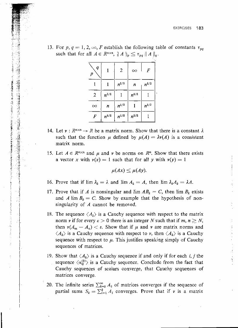
EXERCISES 183

14. Let v : Rnxn -+ R be a matrix norm. Show that there is a constant 3L such that the function ,u defined by ,u(A) = Av(A) is a consistent matrix norm.

15. Let A E PXn and ,u and v be norms on Rn. Show that there exists a vector x with V ( X ) = 1 such that for all y with v (y ) = 1

16. Prove that if lim Ak = 3L and lim Ak = A, then lim AkAk = AA.

17. Prove that if A is nonsingular and lim ABk = C, then lim Bk exists and A lim Bk = C. Show by example that the hypothesis of nonsingularity of A cannot be removed.

13. For p, q = 1,2, GO, F establish the following table of constants z,, such that for all A E Rnxn, 1 1 A ( I p 5 zpq ( 1 A \ I y .

\ 2

18. The sequence ( A k ) is a Cauchy sequence with respect to the matrix norm v if for every E > 0 there is an integer N such that if m, n 2 N, then v(A, - A,) < E . Show that if ,u and v are matrix norms and ( A k ) is a Cauchy sequence with respect to v, then ( A k ) is a Cauchy sequence with respect to ,u. This justifies speaking simply of Cauchy sequences of matrices.

19. Show that ( A k ) is a Cauchy sequence if and only if for each i, j the sequence (a$') is a Cauchy sequence. Conclude from the fact that Cauchy sequences of scalars converge, that Cauchy sequences of matrices converge.

20. The infinite series C;dAk of matrices converges if the sequence of partial sums Sk - ~ f = , A i converges. Prove that if v is a matrix

184 4. NORMS, LIMITS, AND CONIIITION NUMBEFS

; 4 .. norm and CT=, uk is a convergent series of scalars such that v(AX) 5 uX (k = 0, 1, 2, . . .), then Cy=o Ah- converges.

t

, 3 1

21. Let #(z) = CKdyxz%e a pocver series with radius of convergence Q . i < :

Let A E RnXT2. Show that if, for any consistent matrix norm v, ..4 d v(A) < e, then the series CEO y,Ak converges. [The limit of the series ; +$ 4

is written $(A).] i ? i L.

! f 22. Let A E RnXn and define eA = CEO Ak/k!. Prove that if AB = BA, j ,>

1 then eA+B = eAeB. i i

t NOTES AND REFERENCES

The concept of norm has long been used in functional analysis; its application to matrix theory is more recent. Details and further references are

I I f

given by Householder (1964, Chapter 11), who has done much to popularize the use of norms in analyzing matrix process. Mention should also be made

I of Bauer's "Theory of Norms" (1967), which unfortunately is available

I t

only as a report. i /

In many papers matrix norms are used only for square matrices of a fixed order. Since the product is always defined among such matrices, it

I i

is customary to add consistency as a property of a matrix norm, a usage which conflicts with our definition.

I i

The notion of a family of norms appears to be new. It is merely a ter- 1 minological device for saying in a precise way what everyone knows anyway. i

Theorems 1.9 and 2.7 require compactness arguments for their proofs, i but are not otherwise very difficult. A proof of Theorem 1.9 may be found i

t in the book of Issacson and Keller (1966). ,

i

a

3. INVERSES OF PERTURBED MATRICES i

In this section we shall consider the following problem. Let A E RnXn be nonsingular and let E be an M x~z matrix that is presumed to be small. How small must E be so that the perturbed matrix A + E is also nonsingular, and by how much does ( A + E)-I differ from A-I? In answering r

these questions we shall use the theory of norms developed in the last two sections to make precise the phrases "how small" and "how much."

One application of our results is to the computation of matrix inverses. In Section 3.5 we indicated that the computed inverse of a matrix A would often be near the exact inverse of a slightly perturbed matrix

3. INVERSES OF P E R T U R B E D M A T R I C E S 185

A + E. However, this result does not guarantee the accuracy of the computed inverse, for A-I and (A -t E)-l may differ greatly. In the terminology of Section 2.3 such a matrix would be called ill conditioned with respect to inversion. Our analysis not only gives conditions under which A is ill conditioned, but it also associates with A a condition number that measures the degree of its ill-conditioning.

In order to speak rigorously 'about the sizes of errors involving vectors and matrices, we introduce the following generalizations of absolute and relative error.

D E Fl NITION 3.1. Let A, B E Wmxn with B regarded as an approximation to A. The residual of B is the matrix

If v : WmXn + R is a norm, the error in B with respect to v is the number

v(A - B).

If A # 0, the relative error in B with respect to v is the number

Where it will cause no confusion, we drop the phrase "with respect to v" and refer simply to the error or the relative error. The notions of residual, error, and relative error are of course defined for n-vectors regarded as n x 1 matrices.

EXAMPLE 3.2. On a given computer suppose that the rounded value of a number p is fl(P) = P(1 + Q), where I Q ( 5 Let A E Wmxn and let a be the magnitude of the largest element of A. Let B be obtained from A by rounding the elements of A. Then B = A + E, where

Hence

I1 E llm 5 I1 A l lm lo-t,

and


that is, the relative error with respect to the cm-norm in a matrix rounded to t figures is not greater than

The definition of error and relative error uses the notion of a norm to combine information about a set of numbers into a 'single number. It is not surprising that we should lose information in the process. For example, a small component of a vector with a low relative error may have a high relative error. Moreover, a change of norm may change the relative error markedly.

EXAMPLE 3.3. Let

and

Obviously C is a fairly good approximation to A, while B has a relative error of unity in its (2,2)-element. In spite of this both matrices have a relative error of about 10-4 with respect to the oo-norm. On the other hand, if we introduce the norm v defined by

then

while

Thus the norm v exposes the inaccuracy in the (2,2)-element of B.

Example 3.3 indicates the necessity of choosing a norm to fit the problem, or alternatively, of scaling the problem to fit the norm. In applications to linear systems, the problem of choosing a norm is closely related to the scaling problems we discussed at the end of Section 3.5. Fortunately,

3. INVERSES OF PERTURBED MATRICES 187

in many cases the choice of norm is perfectly evident, as it was in Ex- ample 3.3.

We now turn to the question of the accuracy of perturbed inverses that was raised at the beginning of this section. We shall answer the question by exhibiting a bound on the relative error in ( A + E)-l. For the rest of this and the next section all matrices will be assumed square of order n. The symbol 1 ) ( 1 will denote both a consistent matrix norm on Rnxn satisfying

IIIII = 1 (3.1)

and a vector norm on Rn that is consistent with the matrix norm 1 ) 1 1 ; that is, J J Ax ( 1 5 1 1 A 1 1 1 1 x 1 1 . It should be noted that the results of this section depend critically on (3.1). In particular, they hold for the I-, 2-, and ca-norms, but not for the Frobenius norm.

We begin by considering perturbations of the identity matrix.

THEOREM 3.4. If ( 1 P ( 1 < 1, then I - P is nonsingular, and

PROOF. Let x # 0. Then

since 1 - I ] P I ( > 0. Hence if x # 0, then ( I - P)x # 0, and I - P is nonsingular.

Now from the equation

it follows that

( I - P)-I = I + P(I - PI-?

Hence

I 1 ( I - PI-I I 1 5 I 1 I I 1 + I 1 p I 1 I 1 ( I - P)-I 1 1 . (3.4)

Since / I 1 ) I = 1, the inequalities (3.4) and (3.2) are equivalent. . I

For the identity matrix, Theorem 3.4 answers the first question raised at the beginning of this section; namely how small must P be so that I - P


is nonsingular? The answers to the second question of the proxinlity of ( I - P)-l to I-I = I is contained in the following corollary.

COROLLARY 3.5. If ( 1 P ( 1 < 1, then

PROOF. From (3.3) we have

I - ( I - P)-I = -P(I - P)-l.

Hence

For very small P, the term ( 1 - 1 1 P 11)-I in (3.5) does not differ significantly from unity and the right-hand side of (3.5) becomes effectively 1 1 P ( 1 . In other words, the error in the inverse of a slightly perturbed identity matrix is roughly of the same order as the perturbation.

Corollary 3.5 can be used to estimate the error in the inverse of a perturbed matrix. Actually, a slightly more elaborate result will prove useful later.

THEOREM 3.6. Let A be nonsingular and let 1 1 A-lE 1 ) < 1. Then A + E is nonsingular and ( A + E)-l can be written in the form

where

Moreover

PROOF. Since

A + E = A(I + A-lE)

and I J A-lE l j < 1 , it follows from Corollary 3.4 that ( I + A-lE), and hence A $ E, is nonsingular. Moreover

3. INVERSES OF PERTURBED MATRICES 189

If we define F by I + F = ( I -t- A-lE)-l, then this equation is equivalent to (3.6), and by Theorem 3.5 (with P = -A-lE) we have

Finally, from (3.6),

so that

which is equivalent to (3.8).

Recall that if the approximation P to a has a relative residual Q, then P = (1 - @)a. Equation (3.6) is quite analogous, and it is not out of place to call the matrix -F the relative residual of (A + E)-l as an approximation to A-l. Accordingly, we should expect that I ( F 1 1 wo.uld be the relative error in (A + F)-l; and indeed, comparing the inequalities (3.7) and (3.8), we see that I ( PI( and ( 1 A-l - (A + E)-l ( ) / I 1 A-l I), which is the relative error in (A + E)-l, have the same upper bounds.

If I ( A-lE ) I is significantly less than unity, then the term (1 - I ( A-lE )()-l in (3.8) is essentially unity and the relative error in (A + E)-l is approximately bounded by ( 1 A-lE 1 1 . This suggests that if A-l is very large, the error E in A may be magnified considerably in the inverse of A + E. The following trivial corollary of Theorem 3.6 makes these considerations precise.

COROLLARY 3.7. In Theorem 3.6, let

If 1 ) A-I 1 1 1 1 E ( 1 < 1, then

I 1 r'll 5

and

190 4. NO-RMS, LIMITS. A N D CONDITION NUMBERS

PROOF. We have

If this upper bound is substituted for 1 1 A-lE I] in (3.7) and (3.8), there result the inequalities (3.10) and (3.1 1). .

The left-hand side of (3.1 1) is the relative error in (A + E)-l. If E is sufficiently small, the right-hand side is effectively %(A) ( 1 E l(/J( A ( 1 . Since ) I E 1I/Jj A 1 ) is the relative error in A + E, the inequality (3.1 1) states that the relative error in A + E may be magnzFed by as much as x(A) in passing to (A + E)-l. For this reason, %(A) is called the condition number of A with respect to inversion (and with respect to the norm 1 ) (I). If %(A) is large, then the inverse of A is sensitive to small perturbations in A, and the problem of computing the inverse is ill conditioned. Incidentally, note that %(A) is indeed a magnification constant, for

EXAMPLE 3.8. Suppose that we are given a t-digit approximation B to A, in the sense that ( 1 A - B I ( / ( / A 1 ) " If %(A) = lop, then the relative error in B-I will be approximately and if the elements of A-l are about equal in magnitude, they will be accurate to about t - p digits. In other words, if %(A) = lop, we may expect to lose roughly p significant figures in inverting an approximation to A.

It should be stressed that Corollary 3.7 is weaker than Theorem 3.6, since it is based on the inequality

For random perturbations E, the inequality (3.12) will usually be almost an equality. However, if E has special properties, then Theorem 3.6 may give much sharper bounds than Corollary 3.7. For example if E = EA, where 1 E 1 < I, then Theorem 3.6 gives

EXERCISES 191

while. Corollary 3.7 gives

Obviously (3.13) is the better bound. We conclude this section by completing the proof of Theorem 2.12.

THEOREM 2.12.3. If A is nonsingular and lim Ak.= A, then, for all sufficiently large k, A, is nonsingular and lim Akl = A-l.

PROOF. Let Ek = Ak - A. Then lim ( 1 E, ( 1 = 0. Hence lim ( 1 A-lE, 1 ) = 0. Thus for all sufficiently large k, I ( A-lEk 1 1 < 1 , and by Theorem 3.6, Ak = A + Ek is nonsingular. Moreover, Ail = ( I + Fk)A-l, where

I ( Fk ( 1 ( 1 ) A-lEk ) ( / ( I - ) I A-lEk ( I ) . It follows that lim ( 1 Fk ) I = 0 and hence

lim Ail = lim(I + Fk)A-I = A-l. . EXERCISES

1. Let A and B be of order n with A nonsingular, and let B be regarded as an approximation to A. Define the left relative residual of B as the matrix F = ( A - B)A-I and the right relative residual of B as the matrix G = A-l(A - B). Show that B = ( I - F)A and B = A(I - G).

2. Let A, E E Rnxn with 1 ) EA-I ) I < 1. Prove that A + E is nonsingular and that there is a matrix G satisfying 1 1 G ) I ( 1 1 EA-I II/(l - 1 ) EA-I 1 ) ) such that ( A + E)-I = A-l(I + G).

3. Let A, B E Rmxn and let A have linearly independent columns. Show that it is possible to define a left relative residual F of B as an approximation to A so that B = ( I - F)A. [Hint: A has a left inverse (ATA)-lAT (cf. Exercise 1.6.8).] What can be said if A has linearly independent rows?

4. Prove that if I ( P 1 1 < 1 , then the Neumann series I + P + P2 + . converges to ( I - P)-l. Use this to give an alternate proof of Theorem 3.4 and Corollary 3.5.

5. Show that if P is sufficiently small, then (I - P)-l ( I + P) in the sense that I ( I + P) - ( I - P)-l ( 1 ( 2 I ( P 112. Conclude that the bound (3.5) is sharp.

192 4. NORMS. LIMITS, AND CONDITION NL'MBERS

6. Prove that the matrix F of Theorem 3.6 is given by the infinite series

F = --A-lE[I - A--lE + (A-lE)2 - . . . I .

Hence derive the bound (3 .7) and conclude that it is sharp.

7 . Let

For

compute the relative error in ( A + E)-l. Also compute the error predicted by (3.8) and (3.11). Do the same for

Explain any disparity in the results.

8. Explain under what conditions the inequality (3.12) may be expected to be nearly an equality when the elements of E are random.


The perturbation theory of this section is classical and goes through for bounded operators in a Banach space. The theorems are usually established by means of the Neumann series

The condition number [ I A ) I 2 I( A-I ) I 2 first appears in the rounding-error analysis of von Neumann and Goldstein (1947) in a somewhat disguised form. Turing (1948) seems to have been the first to use the term condition '

number, which he defines in terms of matrix norms as is done in the text.

4. THE ACCURACY OF SOLUTIONS OF LINEAR SYSTEMS

In Section 3.5, we saw that the computed solution -7 of the nonsingular system of linear equations

Ax - b (4.1

4. THE ACCURACY OF SOLUTIONS OF LINEAR SYSTEMS 193

satisfies the equation

(A + E)X = b,

where E is in some sense small. However, the computed solution Z will be accurate only if the problem of solving (4.1) is well conditioned in the sense of Section 2.1. In this section we shall derive bounds for the error in X as a function of E. As in the last section, the bounds will depend on the condition number x(A) defined by (3.9).

Since bounds on the matrix E in (4.2) are known, it is possible to combine them with the bounds of this section to bound the error in X. Given a condition number for A, this bound can be computed without computing 2. Such an error bound is called an a priori bound. I t is not unreasonable to suppose that if we compute 2, the additional information obtained in the course of the computations can be used to obtain a better bound. Such a bound that depends on the approximate solution itself is called an aposte- riori bound. We shall discuss a posteriori bounds for the errors in approximate solutions of (4.1) ; however, the results are, in general, disappointing.

The first problem we shall consider is that of assessing the effects of a perturbation in the vector b on the solution of (4.1). So far as rounding- error analysis is concerned, this is not a very important problem, since the effects of rounding error can be accounted for by perturbations in A alone. In practice, however, the components of b may be contaminated with errors-perhaps they themselves have been computed with rounding error-and it is important to have a bound for the error induced in the solution.

Specifically suppose that 6 is an approximation to b and jS is the solution of the system

AX = 6. Then

x - x = ~ - l ( b - 6),

and hence

( I x - n ll 5 ll A-I I1 I1 b - 6 l l . (4.3)

The inequality (4.3) already suggests that if 1 1 A-l )I is large, then the error in X may be significantly greater than the error in 6. We can make this more precise by computing the relative error in the solution. From (4.1) it follows that


Hence

If, as in Section 3, we define %(A) = 1 ) A ) I 1 1 A-l 11, then our results may be summarized in the following theorem.

THEOREM 4.1. Let A be nonsingular, Ax = b # 0, and AX = 6. Then

where %(A) = 1 ) A ) I ( 1 A-l 1 1 .

This theorem requires two comments, In the first place, the condition number %(A) plays much the same role as it did in Corollary 3.7; the relative error in b may be magnified by as much as a factor of %(A) in the solution. The second comment is that when A is ill conditioned the result is frequently unrealistic, since the lower bound (4.4) on I ( x 1 1 is often a severe underestimate. In fact for most right-hand sides b,

where y < 1 is a constant near unity. If this estimate is used in place of (4.4), the result is

so that the relative error jS is hardly greater than the relative error in 6. If x and b satisfy (4.5) with y near unity, then they are said to reflect the condition of the matrix A. Our observation is, then, that a problem that reflects the condition of A is insensitive to perturbations in b, even if % ( A ) is large.

Either Theorem 3.6 or Corollary 3.7 may be used to estimate the error in the solution of (4.2), with Corollary 3.7 giving a weaker result. We state both results.

THEOREM 4.2. Let A be nonsingular, let x # 0 satisfy (4.1), and let 3 satisfy (4.2). If 1 1 A-lE 1 1 < 1, then


If )I A-I I j 11 E 11 c 1, then

PROOF. Since I( A-lE ( 1 < 1, by Theorem 3.6 the matrix A + E is non- ! singular and (A + E)-l = (I + F)A-l, where F satisfies (3.7). Then a !

1

where

I1 l I m 5 +(n) II A 11,

Hence

If (3.7) is used to estimate F, then (4.6) results. If (3.10) is used, then (4.7) results. .

It is interesting to note that the bounds are independent of the right- hand side b. The number x(A) again serves as a condition number in (4.7), telling how much the relative error in A is magnified in the solution. Unless 1 ) A-lE 1 ) << 1 ) A-l 11 1 1 E 11, which is unlikely for random perturbations, the bounds (4.6)'and (4.7) will give comparable results. Moreover, these bounds will be sharp if 1 ) Fx ( 1 1 1 F 1 1 Jl x 11, which will usually be true. This con- trasts with the bound in Theorem 4.1 which is likely to be an overestimate when A is ill conditioned.

These bounds may be combined with the results of Section 3.5 to yield rigorous bounds on the accuracy of computed solutions of linear equations. For example, provided there is no growth in the elimination process, Theorem 3.5.3 may be interpreted as saying that the computed solution X of (4.1) satisfies

(A + H)T = b, (4.8)

Here $(n) is a function of n whose form depends on the arithmetic details


of the computation, but which in any event is not very big. If

then the condition j l A-* 11, 11 H 11, < 1 is satisfied, and Theorem 4.2 applies to show that

Recalling Example 3.8, we see that if +(n) is not too large and x(A) = lop, then we may expect a solution computed in t-digit arithmetic to be accurate to about t - p significant figures, a t least when there is no severe imbalance in the sizes of the elements.

We turn now to the problem of calculating a posteriori bounds for an approximate solution X of (4.1). A natural check on ji. is to substitute it into Equation (4.1) and see to what extent it fails to satisfy the equation. This amounts to looking at the size of the residual vector

If r is zero, then X is an exact solution of (4.1). If r is small, it might be expected that 3 is near a solution of (4.1). The following theorem states precisely in what sense this is true.

THEOREM 4.3. Let A be nonsingular and Ax = b # 0. Let X be given and set r = b - AX. Then

PROOF. We have

Hence

II x - 3 I 1 5 1 1 A-I I I I/ r 1 1 . However,

If (4.1 1 ) is divided by (4.12), the result is (4.10).


As a practical means for assessing the accuracy of an approximate solution, Theorem 4.3 is somewhat disappointing; for it asserts that the accuracy of the solution depends not only on the size of the residual but also on the condition number of the matrix. If A is ill conditioned, even a very small residual cannot guarantee an accurate solution. Worse yet, it is possible for an accurate solution to have a large residual. These points are illustrated in the following example.

EXAMPLE 4.4. Let A = (1.000 1.001)

1.000 1.000

and b = (2.001, 2.000)T. Then the exact solution of the equation Ax = b is x = (1, However, the vector X = (2, O)T, which is in no sense near x, has the very small residual vector r = O)T.

On the other hand, the solution of Ax = b = (1, O)T is x = (-1000, 1000)T, and the vector X = (-1001, 1000)T is very near x. However, the residual vector of 3 is r = (0, -1) which is as large as b.

Further insight into the nature of the residual may be gained by considering the residual of a rounded solution X of (4.1). From Example 3.2 we know that X may be written in the form X = x + e, where 1 1 e I(, (

( 1 x 11, Hence

Now if A is ill conditioned and x reflects the ill-conditioning of A, so that 1 1 x / Im is large, then r will be large. In other words, the rounded soltrtion of an equation may have a large residual. This phenomenon is illustrated by the second part of Example 4.4.

It is also instructive to compare the residual of the rounded solution 2 of (4.1) with the residual of the solution X computed by, say, Gaussian elimination. We know that X satisfies (4.8), where H satisfies (4.9). Hence r = b - A E = H Z , or


If $(n) is ,lot too large, the bound (4.14) is comparable to (4.13). Thus the residual of the computed solution will be roughly of the same size as the residual of the exact solution rounded to t figures. Note that if A is ill conditioned and jE does not reflect the ill-conditioning of A, then ] / X ((, will be small, say of order unity, and 11 r (1, will be of order This can happen even when jE is inaccurate in all its significant figures.

So far all our bounds have the defect that they depend on the condition number of the matrix A and hence on A-l. Since the calculation of inverses is relatively expensive, it is natural to ask how one can detect ill-conditioning without computing A-l.

One sign of ill-conditioning is the emergence of a small pivot in the reduction of A. For example, the Crout reduction decomposes A into the product LU, where the diagonal elements of L are the pivots. If one of these diagonal elements is small, .then L-l will be large. In all probability A-1 = U-IL-1 will also be large, and hence A will be ill conditioned. For

most matrices this is a fairly reliable indicator of ill-conditioning, especially if complete pivoting is used. However, there do exist ill-conditioned matrices for which no small pivots emerge.

A second sign of ill-conditioning is the emergence of a large solution. Suppose, for example, that ) ( A 1 ) = 1 ) b.11 = 1 . Then if Ax = b, we have

so that if I ( x ( 1 is large, %(A) must perforce be large. Unfortunately, an ill-conditioned system may have a small solution. Note that such a solution must also have a very small residual.

It would seem then that the only sure way of detecting ill-conditioning is to compute an approximation to A-l. Actually, for full matrices this is not entirely out of the question, for if an LU decomposition of A has already been computed at a cost of n3/3 multiplications, the decomposition A-1 = U-IL-I may be computed for another n3/3 n~ultiplications. Thus for

twice the work one can compute the upper bound 1 1 U-l )I 1 1 L-l 1 ) on ( 1 A-l I(. A cautious person might feel the additional work is not too high a price to pay for the security of knowing when his problems are ill conditioned. However, in the next section we shall consider a method for improving approximation solutions from which a fair estimate of the condition of the problem may be obtained.

EXERCISES 199

EXERCISES

1. Let A E Rnxn be nonsingular and let X be an approximation to A-l. Define the residual matrix R by R = I - AX. Show that

Compare this result with the corresponding result for linear systems.

2. In Exercise 1 show that

Hence conclude that a matrix X can be a good approximate right inverse for A but a bad approximate left inverse.

3. Give an example of an ill-conditioned matrix A and a matrix X for which the bound in Exercise 2 is nearly attained.

4. Discuss the economics of computing A-l to estimate the condition number of A in the special case when A is tridiagonal; upper Hes- senberg.


The material in this section is covered by Wilkinson (1963) and many others.

Given an approximate inverse X to A one can define, in analogy with the residual vector associated with a linear system, a residual matrix

R = I - AX.

Unlike the residual vector for linear systems, R does reflect the accuracy of the approximate inverse X ; for

hence

However, it should be noted that if A is ill conditioned, its rounded inverse may have a large residual.

200 4. NORMS, LIMITS, AND CONDlTlON NUMBERS

Although it is possible to construct systems of equations that do not reveal any obvious signs of ill-conditioning, such systems do not often occur in practice. Noble (1969) gives a chart of various tests for ill-conditioning.

5. ITERATIVE REFINEMENT OF APPROXIMATE SOLUTIONS OF LINEAR SYSTEMS

In this section we shall analyze a method for improving an approximate solution of the equation

Ax = b, (5.1)

where A is a matrix of order n which is not too ill conditioned, in a sense to be made precise later. The method starts with an approximate solution x, and produces a new approximate solution x, which is nearer x than x,.

" Obviously one can again apply the method to the approximate solution x, to obtain an even better approximation x,. Proceeding in this way, we obtain a sequence (xk) of approximate solutions that converges to the true solution x. A process, such as we have just described, that generates successively a sequence of approximate solutions of a problem is called an iteration. The method to be described in this section is therefore called the method of iterative refinement of an approximate solution of (5.1).

The idea behind the method is simple. Let x, be an approximate solution of (5.1), presumably obtained by the techniques of Section 3.4. Let

r, = b - Ax,

be the residual corresponding to x,. Then if we solve the system

Ad, = r, (5.2)

and calculate

x, = x1 + dl,

it follows that

x, = xl + A-lr, = xl + A-l(b - Ax,) = x, + A-lb - x, = A-lb = x,

so that x, is the exact solution. Note that this procedure is quite cheap; for if the matrix A has been decomposed to compute x,, say by Crout reduction, then it need not be decomposed again to solve (5.2). Since the

5. ITERATIVE REFINEMENT OF APPROXIMATE SOLUTIONS OF LINEAR SYSTEMS 201

computation of the residual requires only n2 multiplications, the whole process can be carried out with 2n2 multiplications.

In practice the computations must be carried out with rounding error, so that x2 will not be an exact solution. In fact, the errors made in solving (5.2) for dl are of the same kind made in solving initially for x , , and it is not at all clear that x, will even be as good an approximate solution as x , . It is .therefore necessary to give a detailed analysis of the process to discover under what conditions x , is an improvement.

Since the analysis is lengthy, we begin by stating its final objective. We shall attempt to exhibit a constant 7 > 0, independent of x , , such that

This being done, it follows by induction that

If we can adjust the computations so that 7 < 1, then lim qk = 0, and it follows from (5.4) that lim xk = x. The result we shall actually obtain is a little weaker than this, but it will still suffice to establish the practical convergence of the method. For notational convenience we shall let the symbol ( 1 1 1 without a subscript denote the 00-norm ) I llm.

The process with rounding error may be described as follows.

I ) r, = fl(b - Ax,) - b - Ax, + el

2 ) dl = fl(A-lr,) = ( A + H,)-l r, (5.5)

3 ) X , = fl(x1 + dl ) + dl + g1

Here the vectors g, and el represent the difference of the true values from the computed values (n.b. el is not the natural basis vector). The matrix HI is the error matrix of Theorem 3.5.3. We have seen (cf. page 195) that if computations are performed in t-digit arithmetic, then

It follows from Corollary 3.7 that if, say,

then

202 4. NORMS. LIMITS, AND CONDITION NUMBERS

where

The first step in the analysis is to obtain a bound for 1 ) el 1 1 in terms of 11 x - x1 1 1 . T o do this let

Note that p, is the relative error in the residual. Now

r, - el = b - Ax, = A(x - xl).

Hence

IIr1 I 1 - I 1 el II i IIA I I Ilx - xl II.

Substituting the value for ( 1 r , I ( obtained from (5.9), we obtain

Now from statements 2 and 3 of (5.9, we have

x - x, = x - xl - (A. + HI)-lr, - g,.

In view of (5.7) and the definition of r,, we have

x - x2 = x - x, - (I + F,)A-l(b - Ax, + el) - g,

= x - xl - (I + F,)(x - x, + A-le,) - g,

= -F,(x - x,) - ( I + Fl)A-le, - g,. (5.1 1)

Taking norms on both sides of (5.1 1) and remembering that I ( F, I( < 1 , we obtain

Finally if the bounds (5.8) and (5.10) are substituted for ( 1 Fl ( 1 and 11 el 1 1 , the result is

5. ITERATIVE REFINEMENT OF APPROXIMATE SOLUTIONS OF LINEAR SYSTEMS 203

If we define x (A)# (n) 1 0-t + 2x(A)Q ' = 1 - ~(A)# (n ) lo -~ I - @ '

then (5.12) becomes

The bound (5.14) is not quite as good as the bound (5.3) since it contains the additional term 1 1 g, 1 1 . However, gl is the error made in adding the correction dl to x,, and unless x, is very near the solution it will be negligible compared to x - x, and x - x,. Thus the problem of convergence is still one of determining when 7 is less than unity.

The first term in the definition of rj is easily disposed of. If x(A) satisfies the restriction (5.6), then by (5.8) this first term is less than unity. Since the polynomial #(n) from the rouding-error analysis is usually an overestimate, the actual bound will generally be a good deal smaller than unity. Thus if A is not too ill conditioned in the sense that it satisfies (5.6), we do not have to worry about the first term.

The second term is another story. Recall that the number e is the relative error in the computed residual. Now we know from the discussion in Sec- tion that if x, was computed as an approximate solution of (5.1), then its residual satisfies

1 1 rl 1 1 5 #(n)lo-t 1 1 A 1 1 1 1 XI 1 1 . (5.15)

On the other hand, when the product Ax, is formed, one of the terms criitjl) will usually be of the same order of magnitude as 1 1 A 1 1 1 1 xl 1 1 . Since by (5.15) the elements of r are almost smaller than aiitjl) one must cancel almost t significant figures when computing r,. This means that if r, is calculated in t-digit arithmetic, the results will be inaccurate in almost their first figure and e will be almost unity. Obviously, 2x(A)e/(l - e), which is .the second term in (5.13) may be much greater than unity.

On the other hand if r, is calculated in double precision (2t digits), the cancellation of t figures will still leave t accurate figures. Thus e will be about and if %(A) satisfies (5.6), the term 2x(A)e/(l - Q) will be less than unity. Notice that double precision should be sufficient for all subsequent iterations of the process, since even the rounded exact solution will not have a residual much smaller than the right-hand side of (5.15). If inner products can be accumulated in double precision, the computation of the residual in double precision will require only single precision multi-


plications. Once the residual has been computed in doubIe precision, it may be rounded to singIe precision and used in statement (2) of (5.5).

Thus if A is not too ill conditioned (this may still be very ill conditioned indeed) and if the residual r, is calculated in double precision, then the error 1 1 x - x, ) I will be smaller than the error ) I x - x, I / . If the process is applied iteratively to generate the sequence of approximate solutions x, , x, , x, , . . . , each xk will have a smalIer error than its predecessor xk-,. This decrease in error will continue to occur until the error is approximately equal to 11 gk ( 1 in (5.14). Practically, since gk is the error made in adding the correction dk to x, , ( 1 g, I ( is approximately equal to 1 1 xk 11 m If 1 1 dk 11 is smaller than this, then dk cannot be added accurately to xk and we may as well terminate the iteration. The resulting approximation x,, will be very near the exact solution rounded to t figures.

We sum up all these considerations in the following algorithm.

ALGORITHM 5.1. Let x be an approximate solution of the equation Ax = b. If A is not too ill conditioned, this algorithm, when performed in t-digit arithmetic, returns in x an approximate solution that is nearly equal to the exact solution rounded to t figures.

1) Compute r = b - Ax in double precision and round to single precision

2) Compute in single precision the solution of the equation Ad = r

3) If ( 1 d JJ,/JI x 11, _( terminate the iteration

4 ) x + - x f d

5) Go to 1

Several comments should be made about this algorithm. In the first place, as it is constructed, it may loop indefinitely if A is too ill conditioned for the iteration to converge. In this case the corrections di will not show a steady decrease but will behave erratically, now decreasing-now increas- ing. Thus it is sufficient to terminate the algorithm with an error stop when

II di IIIII X i + l I I 2 II di-1 I I I I I X i I I - Secondly, we have not yet commented on the speed of convergence.

However, from the approximate inequality

it follows that if q 10-p, then the x, will improve at the rate of about p

$ -"

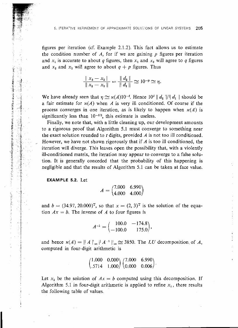
figures per iteration (cf. Example 2.1.2). This fact allows us to estimate the condition number of A, for if we are gaining p figures per iteration and x, is accurate to about q figures, then x, and x2 will agree to q figures

" r & and x2 and x3 will agree to about q + p figures. Thus

We have already seen that q " ~(A)10 -~ . Hence lot 1 ) d, 1 1 / 1 1 dl I ( should be a fair estimate for %(A) when A is very ill conditioned. Of course if the process converges in one iteration, as is likely to happen when %(A) is significantly less than 10-t/2, this estimate is useless.

Finally, we note that, with a little cleaning up, our development amounts to a rigorous proof that Algorithm 5.1 must converge to something near the exact solution rounded to t digits, provided A is not too ill conditioned. However, we have not shown rigorously that if A is too ill conditioned, the iteration will diverge. This leaves open the possibility that, with a violently ill-conditioned matrix, the iteration may appear to converge to a false solution. It is generally conceded that the probability of this happening is negligible and that the results of Algorithm 5.1 can be taken at face value.

EXAMPLE 5.2. Let

i 1 I and b = (34.97, 20.000)T, so that x = (2, 3)T is the solution of the equa- : tion Ax = b. The inverse of A to four figures is I

i i

J and hence %(A) = 1 ) A / I w 1 ) A-l 11, N 3850. The LU decomposition. of A,

I computed in four-digit arithmetic is i i

i 1.000 0.000 7.000 6.990 i .5714 1.000 1 ( 0.000 0.006

Let x, be the solution of Ax = b computed using this decomposition. If I Algorithm 5.1 in four-digit arithmetic is applied to refine x,, there results t the following table of values.

206 4. NORMS, ILIMITS, A N D CONDITION NUMBERS

In the above example X ( A ) I O - ~ Z .4, so that the A is almost too ill conditioned for the algorithm to work. On the basis of this estimate we should expect to gain about half a significant figure per iteration. The actual gain is more like one figure per iteration. The reason for this is that the convergence factor n is approximately equal to ( 1 F I ( where ( I + F)A-I =

( A + E)-l and E is the error made in solving the linear systems. Now most of this error E comes from the error in the LU decomposition, and it is easily verified that I ( A - LU ( 1 3 Thus I ( F 1 1 " 11 A- l , JJ ( 1 E ) /

.8 10-l, which is in accordance with the observed rate of convergence. For the same reason lo4 ( 1 d2 II/I( dl 1 ) 625 is an underestimate for %(A) .

The behavior of the residuals is interesting. The computed solution x1 is inaccurate in all its digits. Nonetheless, the residual is about as small as can be expected, as was predicted in the last section. It is mildly surprising that, although the refined solution x2 is much more accurate, its residual is appreciably larger. This is typical of the process. Although the iterates become more accurate, the residuals do not necessarily decrease. This is to be expected since we have seen in Section 4 that the computed solution x, and the final iterate, which is essentially the rounded exact solution, should have residuals of about the same size. The only way in which the above example is atypical is that the residual corresponding to x4 is zero. This is because x4 is the exact solution whose components happen to be integers.

EXERCISE

1. The method of iterative refinement can be applied to calculate a solution to Ax = b to any desired accuracy. The approximate solutions xi

The method of iterative refinement in the form described here is due to Wilkinson (1963), who analyzes the process for fixed-point arithmetic. Moler (1967) has given a detailed analysis for floating-point arithmetic, which essentially parallels the one given here.

The merits of iterative refinement are not unquestioned. Its critics point out that one must save the original matrix to compute the residual; and anyway it is not worthwhile to try to compute accurate solutions of ill- conditioned problems. In favor of the method it can be said that its slow convergence is a reliable test for ill-conditioning, and for many people that is sufficient justification.

Codes for the iterative refinement of positive definite systems have been published by Martin, Peters, and Wilkinson (1966, HACLA/I/2) and for general systems by Bowdler, Martin, Peters, and Wilkinson (1 966, HACLA/I/7).

EXERCISE 207

must, of course, be accumulated in higher and higher precision, and the residual vector, which will eventually get progressively smaller, must be calculated so that it is accurate. However, there is no point in calculating the residual so accurately that the second term in (5.13) is much less than the first. Assume that an upper bound for %(A) is known and that the computer can operate in t, 2t, 3t, . . . digit arithmetic. Write an algorithm for computing a solution of Ax = b accurate to mt figures.

NOTES A N D REFERENCES

Documents

THE DIRECT SOLUTION OF LINEAR SYSTEMS CHAPTERlya.fciencias.unam.mx/gfgf/sc091/archivos/stewart_chap3n4.pdf · THE DIRECT SOLUTION OF LINEAR SYSTEMS CHAPTER 3 In Theorem 1.6.1 we stated