The Discovery by Data Mining of Rogue Equipment in the Manufacture of

Semiconductor Devices

Steven G. Barbee

A Thesis

Submitted in Partial Fulfillment

of the Requirements for the Degree of

Master of Science in Data Mining

Department of Mathematical Sciences

Central Connecticut State University

New Britain, Connecticut

April 2007

Thesis Advisor

Dr. Daniel Larose

Director of Data Mining Program

The Discovery by Data Mining of Rogue Equipment in the Manufacture of

Semiconductor Devices

Steven G. Barbee

An Abstract of a Thesis

Submitted in Partial Fulfillment of the

Requirements for the Degree of

Master of Science in Data Mining

Department of Mathematical Sciences

Central Connecticut State University

New Britain, Connecticut

April 2007

Thesis Advisor

Dr. Daniel Larose

Department of Mathematical Sciences

Key Words: Radial Basis Function Network, Semiconductor Manufacturing,

Feature Selection, Tree Stump, Tree Curve, Tree Bias

2

Abstract Finding equipment causes of faulty devices in semiconductor manufacturing is inhibited by several difficulties which are briefly described. The main problem area focused on here is that of biased data mining methods. By judiciously selecting two data mining methods from IBM’s data mining workbench, the Intelligent Miner for Data (IM4D), discovery of the known root cause of a decrease in device parametric data from a manufacturing line is more likely to be obtained. The methods employed are the radial basis function network with chi-square ranking for feature selection followed by sequential one-level regression trees (tree stumps) to provide rules. A graphical representation of the rules, the tree curve, is introduced which makes the determination of the root cause visually easy. The value of this approach was proven when it revealed the key candidate for a problem, in IBM’s primary manufacturing line, which was later confirmed by traditional engineering methods to be the root cause.

3

Dedication

This thesis is dedicated to my wife, Debbie, whom I have loved since our teenage years. Her encouragement and support over the past four years allowed me to pursue this degree to completion.

Acknowledgements

I am grateful to the Lord for leading me to a vocational epiphany during my 2001 Christmas vacation which eventually led me to enter this field within IBM. He opened doors, before closing doors, leading me to this chapter in my life. I would also like to thank Professor Larose for creating the online degree program in data mining which quickly brought me up to speed in my second career. His friendly encouragement to me at the end of the 2nd of the first 3 of his courses was especially helpful. I doubt that I would be a data miner today without his encouragement or his foresight and perseverance in providing the world with this resource. My knowledge of data mining was broadened and deepened by the challenging courses of Professors Markov and Dziuda. Professor Markov introduced me to WEKA and machine learning using Prolog and Mitchell’s text. Professor Dziuda introduced me to the fascinating field of gene expression preprocessing and mining for genomics information discovery from microarray data. I would like to thank the above-mentioned professors for serving on my thesis committee.

4

CONTENTS Abstract I. Introduction

A) Goal B) Related Work

II. Semiconductor Device Fabrication A) Introduction B) Definition of Terms

C) Business motivation 1) Implications of Wafer Size 2) Time to Market

D) Data Mining as an Adjunct to Conventional EngineeringIII. Data Mining Challenge A) Scope Limited to Knowledge Discovery (vs. Predictive Analytics)

B) Hierarchical Nature of FabricationC) Variable Reduction and SME BiasD) Complexity of Wafer Trajectories E) Probabilities from the Hypergeometric DistributionF) The Problem of AutocorrelationG) The Problem of Bias in Selection Methods

1) Chi-square 2) Entropy Ranking 3) Information Gain 4) Gain Ratio

5) Gini Index 6) Minimum Description

Length

IV. Data Mining Approach and Application A) Data Exploration B) Data Preparation C) Feature Selection to Reduce Variables vs. Records D) Methods Chosen for Categorical Variables and Numeric Targets 1) Radial Basis Functions a) Applying RBFNs b) Selecting Features with RBFNs 2) Classification and Regression Trees a) Operation of the basic tree method b) Sequential top node method E) Rules for Multiple Process Tools

1) Method for Summarizing and Prioritizing Rules F) Results for Two DatasetsV. Further Study A) Mining Methods B) Feature Creation C) Data Access Limitations Due to Commercial Prudence Appendix A: Acronyms Appendix B: Cited Books Biography of the Author

5

Abstract Finding equipment causes of faulty devices in semiconductor manufacturing is inhibited by several difficulties which are briefly described. The main problem area focused on here is that of biased data mining methods. By judiciously selecting two data mining methods from IBM’s data mining workbench, the Intelligent Miner for Data (IM4D), discovery of the known root cause of a decrease in device parametric data from a manufacturing line is more likely to be obtained. The methods employed are the radial basis function network with chi-square ranking for feature selection followed by sequential one-level regression trees (tree stumps) to provide rules. A graphical representation of the rules, the tree curve, is introduced which makes the determination of the root cause visually easy. The value of this approach was proven when it revealed the key candidate for a problem, in IBM’s primary manufacturing line, which was later confirmed by traditional engineering methods to be the root cause. I. Introduction Before we delve into data mining, we’ll first explore the complicated world of semiconductor manufacturing so that we can better understand the business motivation behind this work. Then we’ll look at technical difficulties, particular to manufacturing, which may hinder our mining or the interpretation of our mining results. Finally, we’ll present different approaches to mining and concentrate on our preferred method and a means of interpreting its results. In the manufacture of semiconductor devices, electrical properties can be affected by deviations in the fabrication process due to drifting or otherwise poorly performing processes or equipment (also referred to as tools). Data mining methods in knowledge discovery can detect which process equipment (tool) may have caused such deviations. However, a naive application of data mining methods may lead to erroneous results due to the presence of bias in the method. The problem may be further worsened by an imbalanced dataset in that there are few wafers (work pieces) with the best electrical characteristics versus a majority with poorer characteristics or vice versa. Logistics, the particular path of the work piece through the manufacturing line, contained in datasets, may frequently present us with as many variables as there are records or instances. Given all of the methods contained in a single data mining workbench, the challenge is then to find the best method, or combination of methods, to discover any equipment causing poor electrical characteristics in the final product (referred to as work pieces, integrated circuits, microchips or semiconductor devices). I.A.) Goal The goal of this work is to find the best discovery method among those available in a given commercial data mining suite to use on such datasets as are common in the semiconductor industry. Since combinations of two or more of the process tools used

6

during semiconductor device fabrication may be causative, the methods must allow for the discovery of such tool combinations. The hypothesis within this work is that a method or combination of methods will overcome a misleading selection bias in this knowledge discovery problem. I.B.) Related Work One of the earliest papers detailing the application of data mining to semiconductor manufacturing applied a tree to process control.1 There is now a growing level of sophistication in the body of literature in the semiconductor data mining field. Perhaps the most impressive recent paper on the application of data mining to semiconductor manufacturing is that from Intel.2 A variety of recently developed data mining methods, both commercial and in-house, were shown to accurately predict the completion date of wafers and the device speed of chips based on electrical parameters tested during earlier steps in their fabrication. Motorola has also published their development of a software application for data mining named CORDEX3 which uses Kohonen self-organizing maps for clustering the data followed by a tree for rule analysis within the clusters. Based on the complexity of data mining methods and the history of the acceptance and use of statistical methods, such as the design of experiments, among the engineering community it is this author’s opinion that the newest, most advanced data mining methods are wielded today by only a select few in a company’s semiconductor manufacturing operation despite the huge ROI realizable when they are properly applied. The use of more generic, but still powerful, methods through user-friendly GUIs in commercial software will best spread the use of data mining among the general engineering community and should be strongly encouraged. The community of data mining companies4 producing specialized software or services customized to semiconductor manufacturing is growing. Trees and neural networks are commonly encountered in such software, the latter for both clustering and prediction. For instance, AMD’s Richard Kittler (formerly of Yield Dynamics) and Weidong Wang (Yield Dynamics) tout the use of Bayesian nets and decision trees;5 they also survey the present and predict the future use of data mining in the semiconductor industry.6

1 “Applying Machine Learning to Semiconductor Manufacturing,” K. Irani, J. Cheng, U. Fayyad, Z. Qian, IEEE Expert, Febr. 1993, pp. 41—47. 2 “Advancements and Applications of Statistical Learning/Data Mining in Semiconductor Manufacturing,” Randall Goodwin, Russell Miller, Eugene Tuv, Alexander Borisov, Mani Janakiram, Sigal Louchheim, Intel Technology Journal, Volume 8, Issue 4, 2004; pp. 325—336. 3 “Data Mining Solves Tough Semiconductor Manufacturing Problems,” Mike Gardner and Jack Bieker, Proc. ACM SIGKDD 2000, Boston, MA, pp.376—383. 4 See, for example, Yield Dynamics’ YieldMine; Neumath: http://www.neumath.com/solutions/solutions_index.htm ; Quadrillion Q-Yield: www.quadrillion.com ; and PDF Solutions: http://www.pdf.com/services_solutions.phtml5 “Data Mining for Yield Improvements,” Richard Kittler and Weidong Wang, Proc. Int’l. Conf. on Modeling and Analysis of Semiconductor Manufacturing, Temp, Arizona, 2000, pp.270-277. 6 “The Emerging Role for Data Mining,” Richard Kittler and Weidong Wang, Solid State Technology, Vol. 42, Issue 11, November, 1999.

7

An example of literature from academia that is closely related to the present work is that of the National Chiao Tung University with TSMC (Taiwan Semiconductor Manufacturing Company)7 where several undisclosed methods were used to back test data mining methods to discover the root cause using data from a semiconductor manufacturing facility. If the results of the data mining method ranked the root cause among its top 5 candidates then the method was deemed to be successful. A similar ranking approach will be used to determine the success of the mining methods used in this work. Back to CONTENTS II. Semiconductor Device (Chip) Fabrication8

II.A) Introduction The manufacture of semiconductor-based devices, integrated circuits or microchips, involves a lengthy and repetitive set of processes often numbering in the hundreds of steps. Each of many (perhaps hundreds of) microchips are formed on a cross-sectional (orthogonal to the axis) slice of a cylindrical crystal of silicon. These slices are known in the trade as “wafers” and are currently as large as 300mm in diameter and over a millimeter in thickness. Batches, or “lots,” of wafers move together in a container from tool to tool, automatically, in the newest factories (also known as foundries, fabricators or “fabs”). Within a tool they may be individually processed in several single-wafer chambers. It is expected that there will be differences in processing from tool to tool and chamber to chamber that may lead to different electrical results in the microchips on the wafers. Furthermore, the processes can vary across the wafer so that there are planar regions of variation so that individual microchips within each wafer may receive slightly different processing. The process steps exercised to form devices on the microchips within a wafer involve various physical and chemical methods to define and form circuit elements such as by chemically doping the semiconductor material to form electrically active regions in transistors, diodes, capacitors comprising memory or logic components within a device in the microchip. II.B) Definition of Terms In knowledge discovery, we search attribute values of independent variables that affect the dependent variable by poring over thousands of instances. We will use any of the following synonyms depending on their context: Independent variable = variable = process (e.g. EQP_A11)

7 “A Data Mining Project for Solving Low-yield Situations of Semiconductor Manufacturing,” Wei-Chou Chen, Shian-Shyong Tseng, Kuo-Rong Hsiao, Chia-Chun Liu, 2004 IEEE/SEMI Advanced Semiconductor Manufacturing Conference, pp.129—134. 8 See, for example, Silicon Processing for the VLSI Era, Vol. 1: Process Technology, 2nd edn., S. Wolf and R. Tauber, Lattice Press, 1999. Volume 2 on Process Integration is also of interest here.

8

Independent variable’s attribute = attribute = tool or equipment (e.g. AE01) Dependent variable = target = electrical parameter % of goal or ratio (e.g. C or LR) Instance = record = wafer = work piece In this section we also introduce common acronyms for process categories (see Appendix A). Semiconductor processes require very complex phenomena such as: (a) ion implantation (ION) where dopant ions accelerated to KeV (or higher) energies become embedded with tightly controlled dosages and depths in well-defined areas of semiconductor materials; (b) reactive ion etching (RIE) where chemically reactive ions from plasmas impinge on masked openings to isotropically or anisotropically remove thin films; (c) chemical vapor deposition where thermally, or plasma (PE), activated chemical species chemisorb and react on surfaces forming thin (as thin as an atomic layer) conformal films, typically insulators (INS), but of any type of material controlled to molecular dimensions in thickness; (d) physical vapor deposition, where the species are sputtered from targets or evaporated from sources to form films by physisorption, that may serve as seed layers or liners (LNR) between metal films; (e) lithography (LTH) which involves exposing photoreactive films to ultraviolet light to define the smallest possible, circuit speed-limiting, widths of areas on the chip; (f) anneals (FRN) where wafers are heated with tightly controlled thermal ramps and temperatures that move or activate dopants or densify films or cause reactions at film interfaces; (g) wet etches to remove thin films (h) cleans where either wet (WET) reagents chemically, or with cryogenic aerosols (AERO), ballistically remove monolayer or particulate contaminants; (i) chemical-mechanical planarization (CMP) where a combination of abrasion and chemical reactions remove films; (j) oxidation where, for Si, a stable silicon dioxide film forms to protect the highly reactive Si surface; (k) stripping of photoresist (RstStrip) by liquid or plasma exposure; (l) metal films are electroplated (MTL) on seed layers to serve as interconnect lines or vias between or within devices on a microchip. The acronyms above have been replaced by an alphabetic encoding that will be seen later in our anonymized data mining results. For example, EQP_A11 might represent the variable for a p-well ION implantation process with attributes (tools) represented by alphanumerics (e.g. AE01). A typical sequence during device formation is to deposit a film, lithographically define a region by projecting the image of a mask, etch the defined regions in the film, deposit a different film or perform an ion implantation. This sequence is repeated many times to define the different regions of the semiconducting device. The different active regions of the device are connected by forming many layers of thin wires connected to each other by vertical conductors or “vias.” Below is a sequence of cross-sections9 that illustrate the large number of steps required, in this case, to form a submicron spacing or opening.

9 S.G.Barbee & G.R.Goth, “Virtual Image Structure for Defining Sub-Micron Dimensions,” IBM Technical Disclosure Bulletin, Vol. 25, No. 3B, August, 1982, p.1448.

9

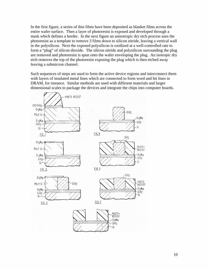
In the first figure, a series of thin films have been deposited as blanket films across the entire wafer surface. Then a layer of photoresist is exposed and developed through a mask which defines a border. In the next figure an anisotropic dry etch process uses the photoresist as a template to remove 3 films down to silicon nitride, leaving a vertical wall in the polysilicon. Next the exposed polysilicon is oxidized at a well-controlled rate to form a “plug” of silicon dioxide. The silicon nitride and polysilicon surrounding the plug are removed and photoresist is spun onto the wafer enveloping the plug. An isotropic dry etch removes the top of the photoresist exposing the plug which is then etched away leaving a submicron channel. Such sequences of steps are used to form the active device regions and interconnect them with layers of insulated metal lines which are connected to form word and bit lines in DRAM, for instance. Similar methods are used with different materials and larger dimensional scales to package the devices and integrate the chips into computer boards.

10

At specific points during the fabrication of complete circuit devices on each wafer, surrogate electrical structures formed in the microchip or in the kerf between microchips are electrically tested to indicate the quality of the product. This in-line testing (ILT) may involve thousands of measurements of voltage, resistance, current, capacitance, transconductance and other properties directly or derived from direct measurements for different structures which roughly emulate components of the circuits in the device. It is especially desirable to predict the electrical performance of the completed chip from these tests at intermediate stages in the chip’s fabrication. The benefit of data mining such electrical tests against wafer logistics is to find rogue tools as quickly as possible before more wafers are misprocessed or out-of-spec by the time they reach the final testing of each chip. The chip fabricator or foundry can then scrap the defective wafers early and replace them by starting more so that committed shipments of working chips to customers can be achieved. Back to CONTENTS II.C) Business Motivation II.C.1) Implications of increasing wafer size and decreasing device geometries. An economy of scale applies to the number of chips per wafer, driving the wafer diameter to increase dramatically over the years from around 25 mm in the late 60s to 300mm in the late 90s. There are few such examples of manufacturing work pieces increasing in size by an order of magnitude over a few decades. Each change to a larger diameter requires building semiconductor processing equipment to accommodate the larger sizes, but more importantly, requires redeveloping the process to maintain the tight control across the much larger surface of the wafer. Unfortunately, certain processes have inherent radial variations for which prior or posterior processes must compensate, if possible. The cumulative effect of such radial nonuniformities can result in a steep degradation of circuit performance or functionality in a radial region of the wafer. Each generation of devices has a shorter gate length across which the charge carriers traverse, so that the switching speed of the transistors is faster (higher GHz) or so that more transistors can be fit into a given chipsize thereby allowing more processors per chip. As chip areas increase so does the chance of large particulates (killer defects) landing on their surface even in pristine clean room conditions. Smaller vertical dimensions typically accompany shorter gate lengths so more precisely controlled thin film forming and removing processes (and tools) are required with each generation. There is always a race to achieve yield on new generations of chips so the pursuit of high yield manufacturing is a continual challenge for the semiconductor foundry. II.C.2) Time to Market The profit incentive is compelling to find rogue equipment preventing rapid yield improvement during this ramp-up stage. The result of one study is that a 6 month delay in ramp-up will reduce profits by two thirds; however, a reduction by 6 months of the

11

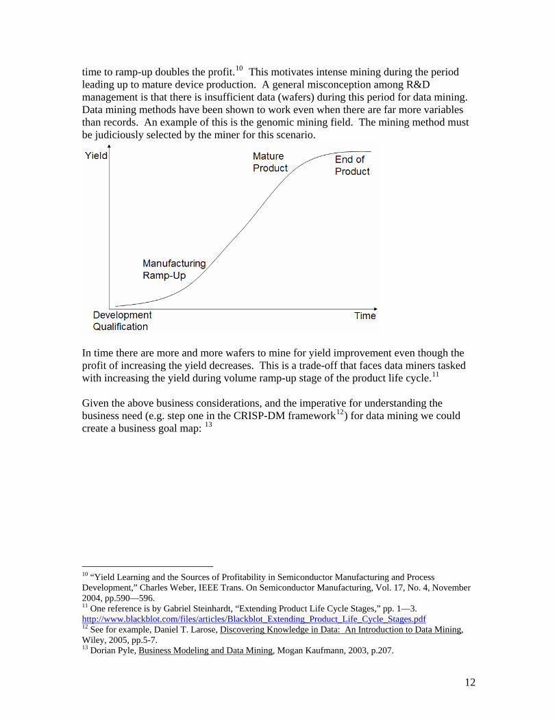
time to ramp-up doubles the profit.10 This motivates intense mining during the period leading up to mature device production. A general misconception among R&D management is that there is insufficient data (wafers) during this period for data mining. Data mining methods have been shown to work even when there are far more variables than records. An example of this is the genomic mining field. The mining method must be judiciously selected by the miner for this scenario.

In time there are more and more wafers to mine for yield improvement even though the profit of increasing the yield decreases. This is a trade-off that faces data miners tasked with increasing the yield during volume ramp-up stage of the product life cycle.11

Given the above business considerations, and the imperative for understanding the business need (e.g. step one in the CRISP-DM framework12) for data mining we could create a business goal map: 13

10 “Yield Learning and the Sources of Profitability in Semiconductor Manufacturing and Process Development,” Charles Weber, IEEE Trans. On Semiconductor Manufacturing, Vol. 17, No. 4, November 2004, pp.590—596. 11 One reference is by Gabriel Steinhardt, “Extending Product Life Cycle Stages,” pp. 1—3. http://www.blackblot.com/files/articles/Blackblot_Extending_Product_Life_Cycle_Stages.pdf12 See for example, Daniel T. Larose, Discovering Knowledge in Data: An Introduction to Data Mining, Wiley, 2005, pp.5-7. 13 Dorian Pyle, Business Modeling and Data Mining, Mogan Kaufmann, 2003, p.207.

12

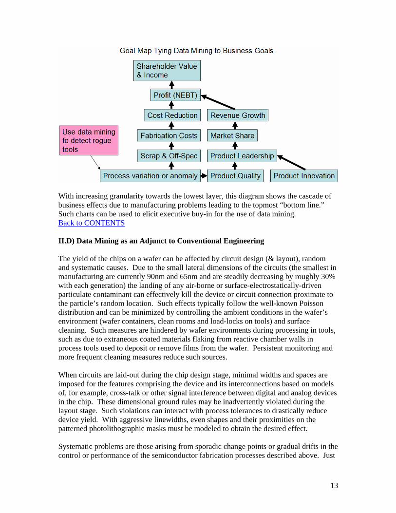
With increasing granularity towards the lowest layer, this diagram shows the cascade of business effects due to manufacturing problems leading to the topmost “bottom line.” Such charts can be used to elicit executive buy-in for the use of data mining. Back to CONTENTS II.D) Data Mining as an Adjunct to Conventional Engineering The yield of the chips on a wafer can be affected by circuit design (& layout), random and systematic causes. Due to the small lateral dimensions of the circuits (the smallest in manufacturing are currently 90nm and 65nm and are steadily decreasing by roughly 30% with each generation) the landing of any air-borne or surface-electrostatically-driven particulate contaminant can effectively kill the device or circuit connection proximate to the particle’s random location. Such effects typically follow the well-known Poisson distribution and can be minimized by controlling the ambient conditions in the wafer’s environment (wafer containers, clean rooms and load-locks on tools) and surface cleaning. Such measures are hindered by wafer environments during processing in tools, such as due to extraneous coated materials flaking from reactive chamber walls in process tools used to deposit or remove films from the wafer. Persistent monitoring and more frequent cleaning measures reduce such sources. When circuits are laid-out during the chip design stage, minimal widths and spaces are imposed for the features comprising the device and its interconnections based on models of, for example, cross-talk or other signal interference between digital and analog devices in the chip. These dimensional ground rules may be inadvertently violated during the layout stage. Such violations can interact with process tolerances to drastically reduce device yield. With aggressive linewidths, even shapes and their proximities on the patterned photolithographic masks must be modeled to obtain the desired effect. Systematic problems are those arising from sporadic change points or gradual drifts in the control or performance of the semiconductor fabrication processes described above. Just

13

the act of improperly performing routine maintenance on a process tool can transform it from the best--yielding to the worst--yielding tool at a given process step. Statistical Process Control (SPC) using Shewhart charts and other means are typical to any manufacturing industry where the performance of the manufacturing tool is tracked through time. When the tool wanders out of specification in its performance corrective action is taken. Advanced Process Control (APC) describes the feeding-forward of departures from the mean for each wafer from a previous process tool to a subsequent one that can correct or compensate for the departure. This is possible for only certain processes and degrees of departure from the mean but is a valuable yield-enhancing practice. The design of experiments (DoE)14 is typically used to find the “sweet spot” of a process in a tool and is commonly used during the development of the manufacturing process. There may be a need for several dependent variables to be optimized and the influential variables do not always have a control knob. Despite any such lurking variables, clever and carefully designed experiments can keep the manufacturing processes away from a cliff. The use of DoE is imperative for developing efficient manufacturing processes, used to fabricate increasingly complex devices, that continue to push the limits of manufacturing science. Diagnosticians of device electrical parametric results and yield often avail themselves of standard ANOVA or Generalized Linear Methods from statistics to determine sources of aberrant results. These methods are well-proven but do not always detect the cause of a problem and may tax the analytical capability of engineers tasked with such responsibilities. This view was put forth by Gardner and Bieker:15 “Quickly solving product yield and quality problems in a complex manufacturing process is becoming increasingly more difficult. The ‘low hanging fruit’ has been plucked using process control, statistical analysis, and design of experiments which have established a solid base for a well tuned manufacturing process.” Based on this author’s observation of job postings by the semiconductor industry and the success of software providers in this area, data mining methods are beginning to be in demand to fill the gaps in the arsenal of those improving device yield in semiconductor fabricators worldwide. Back to CONTENTS III. Data Mining Challenges in Semiconductor Manufacturing In this section we will survey many pitfalls awaiting the data miner or analyst when attempting to discover knowledge in semiconductor manufacturing data. There are a variety of problems, some of which are perhaps unique to manufacturing. Although not

14 A good reference is Design and Analysis of Experiments, 6th edn., Douglas C. Montgomery, Wiley Press, 2005. 15 “Data Mining Solves Tough Semiconductor Manufacturing Problems,” Mike Gardner and Jack Bieker, Proc. of ACM SIGKDD 2000, Boston, MA; 2000, pp.376—383.

14

strictly pertinent to finding a preferred mining method, these problems may still interfere with reaching our goal of discovering knowledge in data in this industrial area. As Professor Mastrangelo has pointed out, “current data mining and analysis techniques do not readily enable modeling of semiconductor manufacturing environments16.” While many mining methods perform well on deep, narrow datasets and there are proven methods for mining shallow, wide datasets such as those found in genomics; we are focused on fairly equal depth and width datasets between these two extremes. With the growth of sensor networks and other input devices, the number of variables pertinent to data analysis is increasing dramatically. With competitive time pressures on the discovery of yield-improving knowledge, the luxury of deeper datasets (i.e., more wafers) is a vanishing possibility for the mining analyst. This work will attempt to demonstrate the performance of two well-known methods in this venue. III.A) Scope Limited to Knowledge Discovery (vs. Predictive Analytics) Data mining encompasses two goals: (1) knowledge discovery from data as well as (2) predictive analytics. The latter typically involves forming a model, or scoring function, from one or a combination of mining methods which are compared by a confusion matrix or gains and ROC charts on how accurately they perform on new data after being trained and then tested on a hold-out dataset. A model is desired which generalizes the behavior of the data and which is therefore not overfit to the training data. The former involves the discovery of data or variable relationships, especially finding the most pertinent variables affecting a target value. This present work is entirely within the purview of knowledge discovery from data (KDD). In our application of KDD, mining methods are successful to the degree that they can discover the cause of reduced performance of integrated circuits (chips). Only process causes are of interest to us; any other causes of poor chip performance are not investigated. The process causes we will investigate are due to rogue process equipment (tools). Since processes and equipment can vary in performance by the: drifting of equipment states; changes in consumables; or frequency and correctly-performed preventive and corrective maintenance. Discovering these altered states of the process is the goal of our knowledge discovery. If equipment sensor data were available, one could conceivably create predictive models for process variation and subsequently, variation in device performance. Back to CONTENTS III.B) Hierarchical Nature of Fabrication There is also a hierarchical nature of the problem in that the wafers are grouped in batches or lots of typically 25—50 wafers and each wafer may have 100 to several hundred integrated circuits (chips). It is quite common that a certain region (e.g. center, 16 “Multivariate Process Modeling: The ‘Preprocessing’ Challenge,” Christina Mastrangelo and David Forrest, pp.1478—1483.

15

top, annulus, outer edge) of the wafer, comprising a percentage of all the chips, is consistently performing or yielding differently than the rest of the wafer’s chips. Although data mining can be performed at the lot or chip level, in this work we will restrict our focus to the wafer level (using the average parameter value of all chips per wafer) of mining. Hierarchies are found in17: i) workpiece groupings; (ii) process & tool state levels; and (iii) electrically testing increasingly complex structures—from kerf to devices on a chip. A reasonable approach to use when ferreting out problems in chip performance due to processing differences is to: (i) Mine a lot-level, wafer-level or chip-regional (quadrant, radii, patterns) performance variable (continuous or discrete classes) against the process steps at the tool or chamber levels to find candidates. Recall that a lot may contain 25-50 wafers, and a wafer may contain 50-100s of chips. (ii) Mine performance data against sensor data (e.g. temperature, pressure, power, chemical flow, step duration) for the top candidate process tools. This adds another layer of granularity below that of tool in the the process / tool / sensor hierarchy. Other consumable and maintenance activities could be added at the sensor level (tool maintenance, chamber conditioning, etc.). (iii) Mine electrical test data of kerf (between chip) structures (such as serpentine intra-level resistor chains) at intermediate metal levels during device interconnect formation as well as functional tests when the chip is completed and when it is packaged. Obviously, the sooner a problem is detected (such as at an early kerf device test) the fewer subsequently started wafers will be affected after fixing the problem compared to having to wait until the chips are at a functional test before mining and problem detection can begin. Back to CONTENTS III.C) Variable reduction and SME Bias As with all other mining applications, guidance from subject matter experts (SMEs) may serve well to exclude variables that are deemed long shots (although this may exclude surprising results) that would be unexplainable for the given outcome. One example would be all of the process steps that occur AFTER the performance parameter is measured (the target variable). Another example would be metrology or test steps prior to that used to obtain the target variable. This practice can greatly reduce the noise level in the data. If this approach fails to reveal a likely candidate, then the entire set of variables can be included. The danger here is that the engineering team may have conceived a physical model (hypothesis) which they hope that data mining will confirm and therefore they have limited the types or sequences of processes that would bring such a result from the input to the data mining model. Even if it does confirm their suspicion, 17 Another very important hierarchy is that in the time dimension. How many weeks or months of logistic data will you mine in an automatic production mode?

16

by excluding the other process steps they may have precluded the discovery of a secondary or even the primary effect. It is very common that data mining will present candidates which are corrected one-at-a-time by the engineering team. Subsequent mining of all of the processes to determine whether previously discarded candidates are persistent, and therefore, real is a reasonable follow-up action. III.D) Complexity of Wafer Trajectories In large manufacturing lines, due to economies of scale, as many wafers are processed as is possible within the confines of the factory floor space. This often requires many duplicate toolsets to perform the same type of process. As we’ve already seen, there are many process steps required to fabricate a device. It would be nice to know the best or worst combination of tools among the steps. Unfortunately, there is a myriad of possible combinations of tools used in the hundreds of fabrication steps. The detection of errant equipment may be further stymied by the need for discovery on relatively few manufacturing work pieces (silicon wafers). As mentioned above, this is especially true during the development of a new product or during the initial stages of product ramp-up when there may be as few as 200 wafers for which pertinent data is to be mined against over 400 process steps with as many as 10 different tools at each step and with a tool containing one or several processing chambers. Considering just tools (not chambers) it is simple to determine the number of ordered samples for a number, r, of consecutive process steps for which there is a selection of a tool from a toolset of size n, with replacement:18 = nr. For example, simplistically assuming that there are only 2 process tools at each of 100 sequential process steps, there are 2 possible paths at the 1st step times 2 possible steps at the 2nd step ... times 2 possible paths at the 100th step = 2100 possible trajectories of a wafer through the 100 steps. More realistically, we could evaluate the scenario where there are over 400 steps with perhaps 50 using 2 tools, 200 using 3 tools, 100 using 4 tools and 50 using 10 tools. Then there are 250 * 3200 * 4100 * 1050 possible unique process-tool trajectories for a wafer. These are almost astronomical numbers. The number is decreased when just unique tools are considered since many types of process step use the same toolset. Even so, these are large numbers. It is quite unrealistic to think that the volume of wafers through a manufacturing line would come anywhere near populating all of these possibilities. For example, if 10,000 wafers were started each day, it would take well over 1046 days (=2.7x1042 centuries) to begin to populate the many process-tool combinations. This makes approaches where a large number of possible combinations is assumed in the population, such as with traditional statistical hypothesis testing methods, quite unrealistic for finding the best or worst overall process-tool trajectories through the entire fabrication of complete devices. 18 See, for example, Probability and Statistical Inference, 6th edn., Hogg and Tanis, Prentice Hall, 2001, p.82.

17

Our focus should rather be on the which tools are bad at particular process steps. Back to CONTENTS III.E) Probabilities from the Hypergeometric Distribution For binary classification where the wafers are partitioned into good vs. bad, defective vs. nondefective (or high vs. low yield) categories, we can find the probability of a tool processing a good or bad wafer. This is an excellent sanity check on the results of a mining model. A useful method for this scenario is to use the hypergeometric distribution19 to find random probabilities, since we are drawing without replacement from a population whose probability of success changes with each draw. If we consider that there are 2 members of the defective class: defective and nondefective. The probability of a tool processing m wafers having k defective wafers where the defective population is n out of a total of N wafers is:

( )( )

( ) ( )

( )

N m !m N m m!m k !k! N m n+k ! n k !k n k

= N!NN n !n!n

⎛ ⎞⎛ ⎞⎛ −⎛ ⎞−⎛ ⎞⎛ ⎞⎜ ⎟⎜ ⎟⎜⎜ ⎟⎜ ⎟⎜ ⎟ − − − −− ⎜ ⎟⎝ ⎠⎝ ⎠ ⎝ ⎠⎝ ⎠⎜ ⎟⎜ ⎟⎜ ⎟⎛ ⎞ ⎜ ⎟⎜ ⎟⎜ ⎟⎜ ⎟ −⎜ ⎟⎝ ⎠⎝ ⎠ ⎝ ⎠

⎞⎟

where: m = the number of wafers processed by a tool k = the number of hypothetical defective wafers processed in a tool n = the number of defective wafers in the population N = the total number of wafers We can substitute the values from the tools at a suspect process step and use either Excel’s COMBIN function or, for larger values, the Hypergeometric Calculator20 to find the probabilities for each tool at the process step. Consider, for example, the distribution of defective (red) and nondefective (blue) wafers distributed among 10 tools as shown in this bar chart21:

Which of these tools would be the most suspicious and, hopefully, selected by our mining analysis?

19 The Wikipedia entry on this topic was used for this section 20 http://stattrek.com/Tables/Hypergeometric.aspx21 Obtained using Spotfire DecisonSite software

18

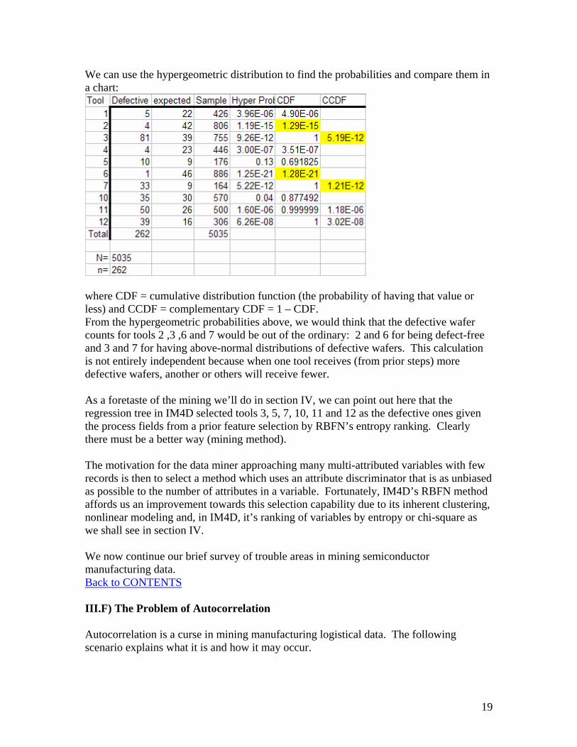
We can use the hypergeometric distribution to find the probabilities and compare them in a chart:

where CDF = cumulative distribution function (the probability of having that value or less) and CCDF = complementary CDF = 1 – CDF. From the hypergeometric probabilities above, we would think that the defective wafer counts for tools 2 ,3 ,6 and 7 would be out of the ordinary: 2 and 6 for being defect-free and 3 and 7 for having above-normal distributions of defective wafers. This calculation is not entirely independent because when one tool receives (from prior steps) more defective wafers, another or others will receive fewer. As a foretaste of the mining we’ll do in section IV, we can point out here that the regression tree in IM4D selected tools 3, 5, 7, 10, 11 and 12 as the defective ones given the process fields from a prior feature selection by RBFN’s entropy ranking. Clearly there must be a better way (mining method). The motivation for the data miner approaching many multi-attributed variables with few records is then to select a method which uses an attribute discriminator that is as unbiased as possible to the number of attributes in a variable. Fortunately, IM4D’s RBFN method affords us an improvement towards this selection capability due to its inherent clustering, nonlinear modeling and, in IM4D, it’s ranking of variables by entropy or chi-square as we shall see in section IV. We now continue our brief survey of trouble areas in mining semiconductor manufacturing data. Back to CONTENTS III.F) The Problem of Autocorrelation Autocorrelation is a curse in mining manufacturing logistical data. The following scenario explains what it is and how it may occur.

19

One scenario is to try to find the tool causing a single bad lot of a product with a small number of wafer starts (i.e. there aren’t many such lots that have finished processing in the manufacturing line). There may be many process steps where an entire lot is processed in a single tool at that step. Each of these single tools is a possible candidate for the anomalous processing of that bad lot. Consider another case where each batch consists of 9 wafers. The order of these 9 wafers is kept in the same sequence within each batch. Suppose that they are processed at steps with 3 tools or a single tool with 3 chambers. Consider also that the loading of the wafers into the tools or chambers is always performed the same way (1st 3 wafers to chamber I; 2nd 3 wafers to chamber II; etc.) at each process step’s tool. Assuming no wafer breakage or culling in previous steps, and no tool unavailability, the clusters of wafers in each batch would have identical process tool histories:

20

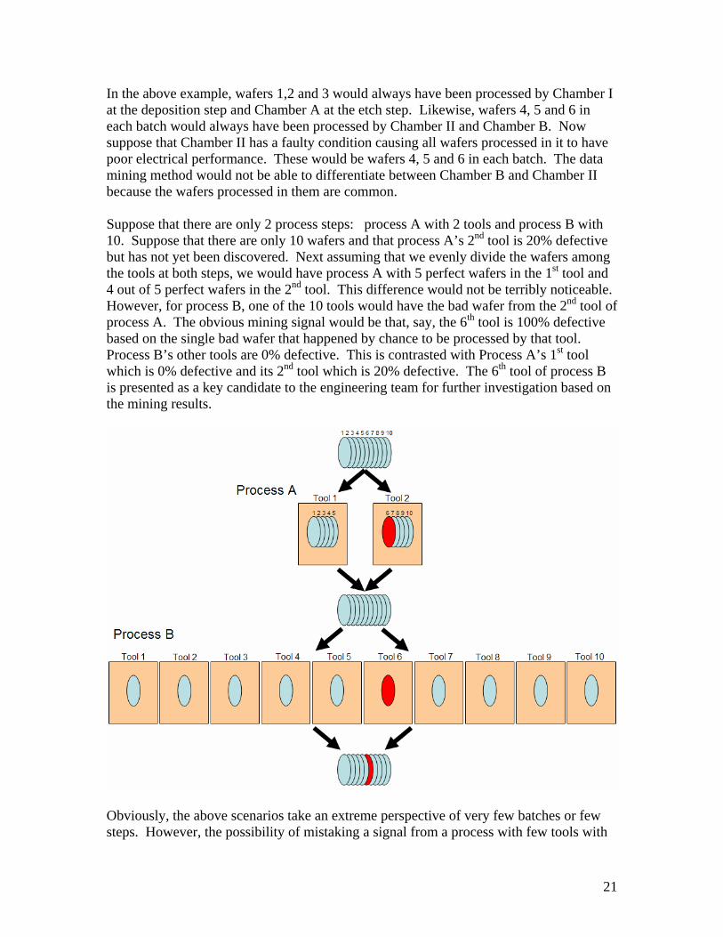
In the above example, wafers 1,2 and 3 would always have been processed by Chamber I at the deposition step and Chamber A at the etch step. Likewise, wafers 4, 5 and 6 in each batch would always have been processed by Chamber II and Chamber B. Now suppose that Chamber II has a faulty condition causing all wafers processed in it to have poor electrical performance. These would be wafers 4, 5 and 6 in each batch. The data mining method would not be able to differentiate between Chamber B and Chamber II because the wafers processed in them are common. Suppose that there are only 2 process steps: process A with 2 tools and process B with 10. Suppose that there are only 10 wafers and that process A’s 2nd tool is 20% defective but has not yet been discovered. Next assuming that we evenly divide the wafers among the tools at both steps, we would have process A with 5 perfect wafers in the 1st tool and 4 out of 5 perfect wafers in the 2nd tool. This difference would not be terribly noticeable. However, for process B, one of the 10 tools would have the bad wafer from the 2nd tool of process A. The obvious mining signal would be that, say, the 6th tool is 100% defective based on the single bad wafer that happened by chance to be processed by that tool. Process B’s other tools are 0% defective. This is contrasted with Process A’s 1st tool which is 0% defective and its 2nd tool which is 20% defective. The 6th tool of process B is presented as a key candidate to the engineering team for further investigation based on the mining results.

Obviously, the above scenarios take an extreme perspective of very few batches or few steps. However, the possibility of mistaking a signal from a process with few tools with

21

that from a process with many tools is only one reason why it is necessary to investigate bias in the mining methods. Back to CONTENTS III.G) The Problem of Bias in Selection Methods A tendency with some mining methods is an inherent bias towards selecting variables with many attributes. This problem has been described in the literature and several methods have been used to try to mitigate it. The fact that there are many approaches and no universal unbiased method should give us pause for concern. After Chi-square, we will briefly list some of the more common selection methods (splitting criteria) from among 16 listed by Maimon & Oded22: III.G.1) Chi-square Simply stated, the Chi-square statistic, χ2, compares the expected to the observed values. The chi-square ranking is based on ranking different variables by the sum of squares their attributes’ departure of observed (O) values from their expected (E) value divided by the expected value:23

( )22 O Eχ =

E−

∑

For the following impurity-based splitting criteria, the following nomenclature and definition holds: given a training set, S, these are the probabilities of the target feature, y: 24

( )1( ) ,..., dom yy cy cy

SSP S

S S

σσ ==⎛ ⎞⎜ ⎟= ⎜ ⎟⎜ ⎟⎝ ⎠

where1y c Sσ = indicates the subset of instances in S for which the feature 1y c= , or the first

instance and dom(y) is the entire domain of features, y. III.G.2) Entropy Ranking25

The entropy ranking is based on the amount of disorder for a given distribution of values of the attributes for a variable:26

2( )

logj

j j

y c

c dom y y c

S SEntropy

S S

σ

σ

=

∈ =

= −∑

22 Oded Maimon & Lior Rokach, “Decision Trees,” Chapter 9, The Data Mining and Knowledge Discovery Handbook, Springer, 2005, pp.168-178. 23 See for example Data Mining: Introductory and Advanced Topics, Margaret H. Dunham, Prentice Hall, 2003, pp.54-55 24 Maimon & Rokach, p.170. 25 See Larose, pp.116-121 for worked-out examples of entropy and information gain. 26 Dunham, pp.98-100.

22

III.G.3) Information Gain Briefly, when the entropy change from one splitting on one variable is smaller than that of splitting by another variable, the information gain is:27

,

, ( )*i i j

i j i

a

dom a

SInformationGain Entropy Entropy

Sυ

υ

σ =

∈

= − ∑

III.G.4) Gain Ratio28

This is merely the information gain divided by the split information to “normalize” it: InformationGainGainRatio

Entropy=

Where the information gain is typically calculated first and then, preferably for appreciable (nonzero) entropy, the Gain ratio is calculated. III.G.5) Gini Index29

2

( )

1 j

j i

y c

c dom a

SGini

S

σ =

∈

⎛ ⎞⎜ ⎟= −⎜ ⎟⎝ ⎠

∑

Back to CONTENTS III.G.6) Minimum Description Length30

The size of the tree is the size of its encoding by bits, and the fewer bits the better. The cost of a split at a leaf t is:

( )

( )*( ) 1 2( ) *ln ln ln

2 2 ( )2

i

i i

t ty c t

c dom y y c t

dom yS dom y S

Cost t Sdom yS

πσ

σ=∈ =

−= + +

⎛ ⎞Γ⎜ ⎟

⎝ ⎠

∑

Where denotes the instances that have reached node t. tS Mitchell31 indicts any method that uses information gain with these comments: “There is a natural bias in the information gain measure that favors [variables] with many [attribute] values over those with few values.” He describes the problem this way: “[the many-attributed variable] has so many possible values that it is bound to separate the training examples into very small subsets. Because of this, it will have a very high information gain relative to the training examples, despite being a very poor predictor of the target function over unseen instances.” He goes on to describe the gain ratio (= 27 Maimon & Rokach, p.174. 28 Maimon & Rokach, p.171. 29 ibid., p.172. 30 ibid., p.178. 31 Thomas Mitchell, Machine Learning, Mcgraw-Hill, 1997, pp.73-74.

23

information gain / split information) as a remedy which unfortunately creates another problem when the split information tends towards zero for a variable. He then references several alternative approaches to resolving this problem. Han and Kamber32 agree with Mitchell and elucidate further in their description of attribute selection methods for trees: “Information gain … is biased toward multi-valued [variables]. Although the gain ratio adjusts for this bias, it tends to prefer unbalanced splits in which one partition is much smaller than the others. The Gini index is biased toward multi-valued [variables] and has difficulty when the number of classes is large. It also tends to favor tests that result in equal-sized partitions and purity in both partitions.” They go on to emphasize Kononenko’s finding33: “[Variable] selection measures based on the Minimum Description Length (MDL) principle have the least bias toward multi-valued [variables].” A popular tree method that claims to mitigate this bias problem is QUEST: 34

“QUEST (quick unbiased efficient statistical tree) addressed the problems in CART that it tends to select variables with many values, which creates a bias in the model.”35

Any mining method with this bias is quickly exposed when applied to semiconductor process logistics data where there are a sizable number of steps with many more tools & chambers than others (e.g. 15 vs. 2). This is a large problem which we address in this work by using feature selection prior to ranking top node competitors in a tree. Back to CONTENTS IV. Data Mining Approach and Application IV.A) Data Exploration Two datasets were created from known causes of electrical test problems. The logistical data for the time period during which the problems manifested was joined to the electrical test data. One is labeled SLMP and the other RX. There are thousands of wafers (instances or records) from electrical tests performed over several months (SLMP) or one month (RX). Dataset Variables Instances Ratio of Instances to Variables SLMP 406 8,193 20.18 RX 208 3,183 15.30 In both datasets, the target or dependent variable is continuous (numeric) and the independent variables are the fields representing the process steps used to fabricate the

32 Jiawei Han and Micheline Kamber, Data Mining: Concepts and Techniques, 2nd edn., Morgan Kaufmann, 2006, pp.304-305. 33 ibid. p.379;, “On biases in estimating multi-valued attributes,” I. Kononenko, Proc. 14th Joint Int. Conf. Artificaial Intelligence (IJCAI’95), vol.2, pp.1034-1040, Montreal, Canada, Aug. 1995. 34 www.stat.wisc.edu/~loh/quest.html35 Dunham, p. 123.

24

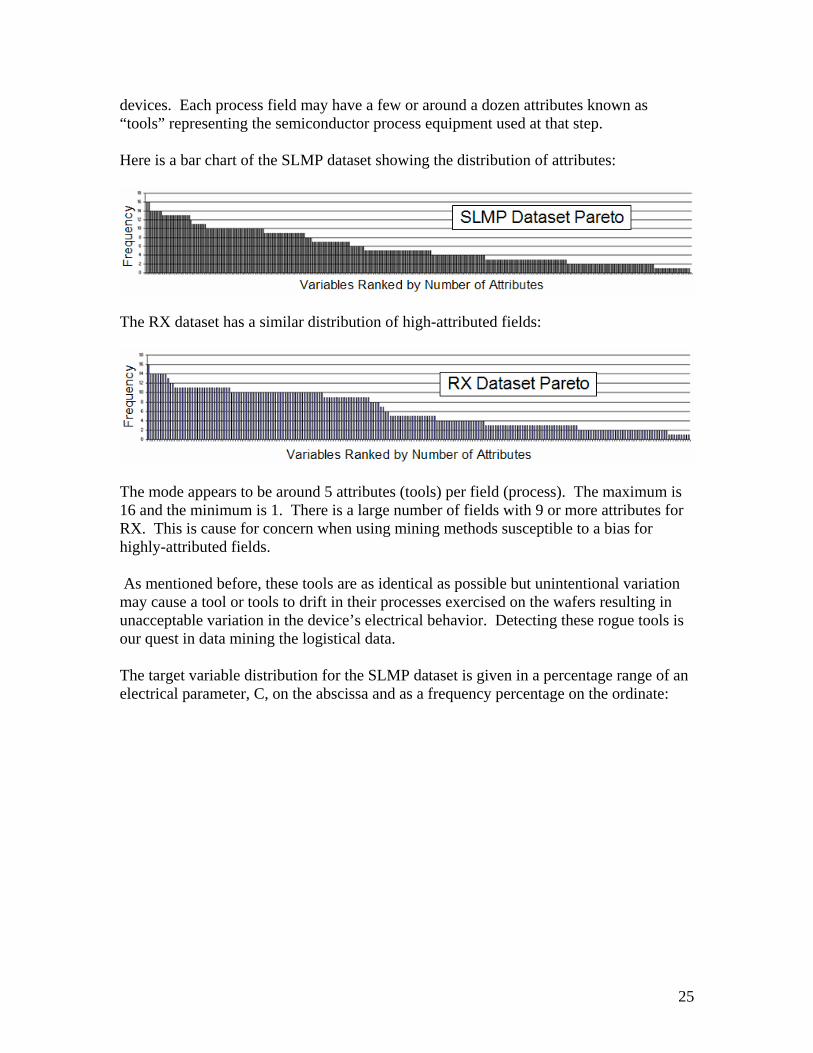
devices. Each process field may have a few or around a dozen attributes known as “tools” representing the semiconductor process equipment used at that step. Here is a bar chart of the SLMP dataset showing the distribution of attributes:

The RX dataset has a similar distribution of high-attributed fields:

The mode appears to be around 5 attributes (tools) per field (process). The maximum is 16 and the minimum is 1. There is a large number of fields with 9 or more attributes for RX. This is cause for concern when using mining methods susceptible to a bias for highly-attributed fields. As mentioned before, these tools are as identical as possible but unintentional variation may cause a tool or tools to drift in their processes exercised on the wafers resulting in unacceptable variation in the device’s electrical behavior. Detecting these rogue tools is our quest in data mining the logistical data. The target variable distribution for the SLMP dataset is given in a percentage range of an electrical parameter, C, on the abscissa and as a frequency percentage on the ordinate:

25

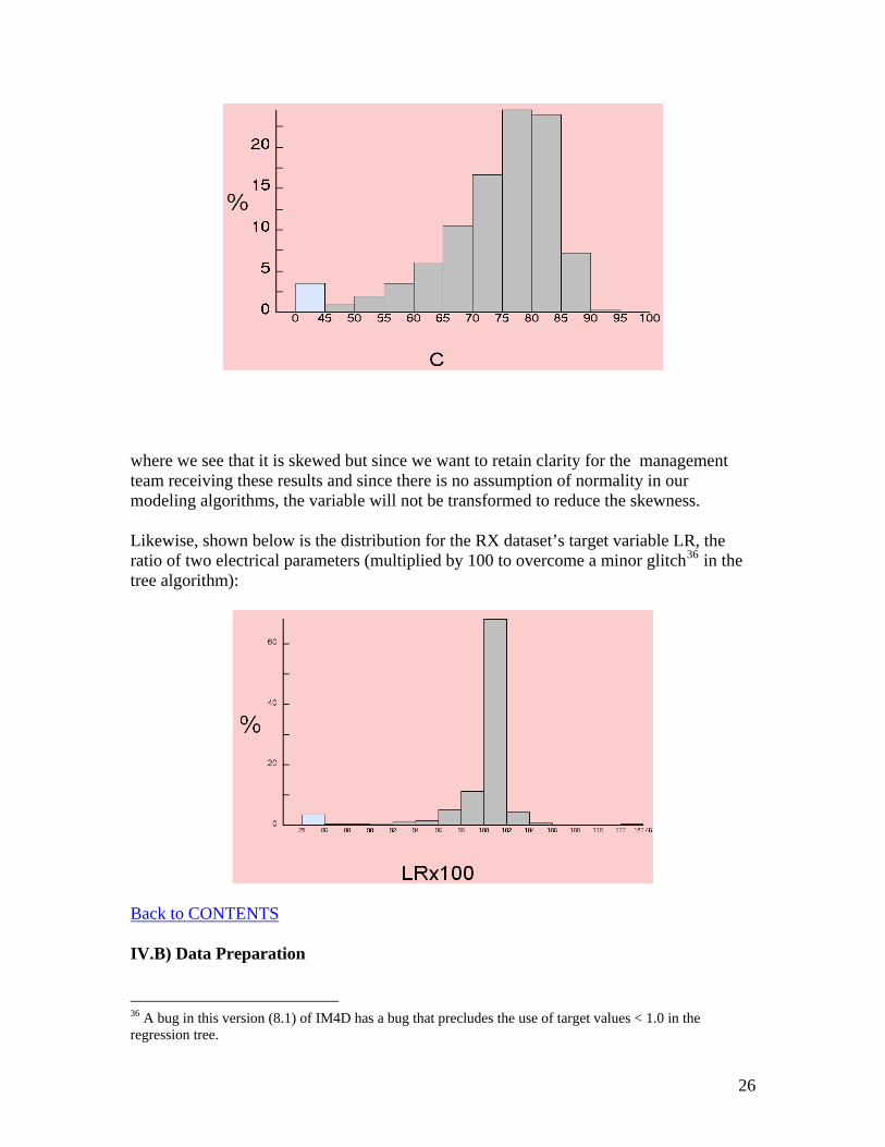
where we see that it is skewed but since we want to retain clarity for the management team receiving these results and since there is no assumption of normality in our modeling algorithms, the variable will not be transformed to reduce the skewness. Likewise, shown below is the distribution for the RX dataset’s target variable LR, the ratio of two electrical parameters (multiplied by 100 to overcome a minor glitch36 in the tree algorithm):

Back to CONTENTS IV.B) Data Preparation

36 A bug in this version (8.1) of IM4D has a bug that precludes the use of target values < 1.0 in the regression tree.

26

As with most data mining investigations, a large effort is required in the preparation of the datasets37 both of which will comprise a month or more of logistics data from the company’s data warehouse joined to electrical parameter data. The datasets are then transformed to formats usable by IBM’s Intelligent Miner for Data and various mining methods are applied to the data. SAS Base software was used to join the logistics dataset to the electrical test dataset; both were obtained from a data warehouse. The joined file was then exported as a CSV file and processed by IM4D’s idmcsv function38 to create data (*.dat) and information (*.info) files which are then read into IM4D using the loadmnb function to create a mining base object. Chip functional or parametric test data was averaged for each wafer. There was no need to filter out subsequent logistical steps with few or no wafers. The range of values for the electrical test had to be within its specifications or the datum was considered as an outlier and culled from the data. Missing data, if excessive (> 25%) could also eliminate a process field from the data. If a step were repeated, only the 1st incidence was used. This excluded experimental processes or processes that were being transitioned to newer, replacement processes. Measurement and testing steps were not included in the logistics fields since they do not affect the structure or functioning of the device. In summary, two datasets were used for this exercise. One (RX) had a single process and tool causing a problem. The other (SLMP) had a group of 5 process steps which all used the same tool within their processes. Back to CONTENTS IV.C) Feature Selection to Reduce Variables vs. Records The reduction of dimension or feature selection entails eliminating inconsequential variables to form a less noisy, more manageable number suitable for most mining methods. This is critical for mining methods that are very sensitive to noise or are computationally intensive (assuming a large amount of data must be crunched). Rules of thumb for the number of variables or records are often suggested by those with experience in using particular data mining methods: “there must be at least six times as many records as variables” or “there must be at least one half as many records as variables for a valid result” and so on. However, these are not easily followed when there are extremes in the number of variables and records. These extremes are sometimes denoted as “wide and shallow” versus “narrow and deep.” The former is a challenge to analytical methods and is encountered routinely in bioinformatics with records on the order of 10 and variables on the order of 10,000. Narrow and deep datasets are routinely

37 Dorian Pyle, Data Preparation for Data Mining, Morgan Kaufman, 1999, p. 11. 38 See, for example, Appendix C (pp.347-353) of Using the Intelligent Miner for Data, version 6 release 1, pub order SH12-6394-00, IBM, 1999.

27

encountered in business applications of data mining. For example, CRM (customer relationship management) or retail sales mining can involve ~100 variables and millions or billions of records. Sampling may be used to reduce the computing time required for such large datasets although not without a penalty.39

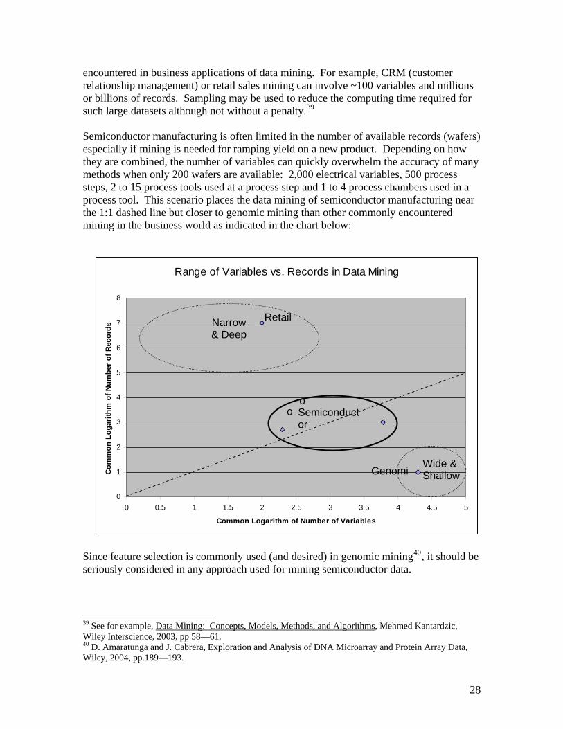
Semiconductor manufacturing is often limited in the number of available records (wafers) especially if mining is needed for ramping yield on a new product. Depending on how they are combined, the number of variables can quickly overwhelm the accuracy of many methods when only 200 wafers are available: 2,000 electrical variables, 500 process steps, 2 to 15 process tools used at a process step and 1 to 4 process chambers used in a process tool. This scenario places the data mining of semiconductor manufacturing near the 1:1 dashed line but closer to genomic mining than other commonly encountered mining in the business world as indicated in the chart below:

Range of Variables vs. Records in Data Mining

0

1

2

3

4

5

6

7

8

0 0.5 1 1.5 2 2.5 3 3.5 4 4.5 5

Common Logarithm of Number of Variables

Com

mon

Log

arith

m o

f Num

ber

of R

ecor

ds Narrow & Deep

Retail

Genomi

Semiconductor

Wide & Shallow

oo

Since feature selection is commonly used (and desired) in genomic mining40, it should be seriously considered in any approach used for mining semiconductor data.

39 See for example, Data Mining: Concepts, Models, Methods, and Algorithms, Mehmed Kantardzic, Wiley Interscience, 2003, pp 58—61. 40 D. Amaratunga and J. Cabrera, Exploration and Analysis of DNA Microarray and Protein Array Data, Wiley, 2004, pp.189—193.

28

A different realm of problems, beyond the scope of this study, is encountered when real-time sensor data (e.g. temperature, pressure, flow, power) from process tools is mined against electrical or defect parameters.41 Various methods are employed in reducing the number of variables in data mining. For instance, WEKA42 has methods ranging from genetic algorithms43 to boosted trees for feature selection. The mining in this work is restricted to IBM’s Intelligent Miner for Data44. The output from the radial basis function is used to find a variable hierarchy. A manageable number of highly-ranked variables are then fed into the tree sequential top node mining method. Back to CONTENTS IV.D) Methods Chosen for Categorical Variables and Numeric Targets IBM’s data mining workbench, Intelligent Miner for Data, IM4D, contains 6 different mining methods: Neural Network (classification or prediction) Radial Basis Function Network (classification or prediction) Association Rules (a priori) Clustering: Kohonen self-organizing map Demographic Classification Tree Perhaps the 3 most popular methods among these are the tree, neural network and association rules. However, in my experience, individually these have had limited success in mining semiconductor logistics data. My preference has been with the radial basis function network, or RBF method but it suffers from a difficulty in ranking and reporting its results. Shown below is the utility of combining two of these data mining methods: the radial basis function network and the classification tree to discover a known root cause of a wide distribution in electrical data. First, we shall offer a “math-lite” overview the topic of radial basis function networks to see where they fit in the arsenal of data mining methods and to get a sense of how they work. IV.D.1) The Radial Basis Function Network 41 PDF Solutions, Proc. AEC/APC Conference, Denver, CO, 2006. 42 Ian Witten and Eibe Frank, Data Mining: Practical Machine Learning Tools and Techniques, 2nd edn, Elsevier, 2005, pp. 420-425. 43 For an example (using WEKA) see D. Larose, Data Mining Methods and Models, Wiley, 2006, pp.252--261. 44 http://www-306.ibm.com/software/data/iminer/fordata/, this particular member of the Intelligent Miner family of products is a standalone workbench and is no longer sold by IBM and will no longer be supported after September 30, 2007.

29

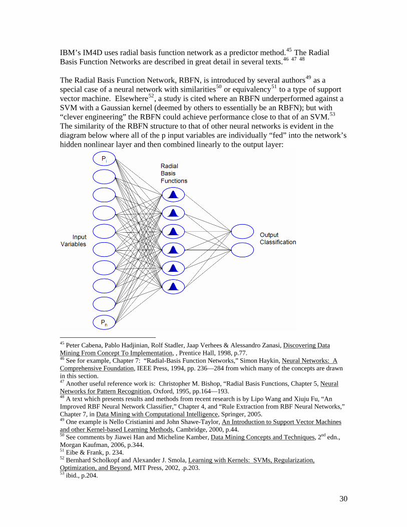
IBM’s IM4D uses radial basis function network as a predictor method.45 The Radial Basis Function Networks are described in great detail in several texts.46 47 48 The Radial Basis Function Network, RBFN, is introduced by several authors49 as a special case of a neural network with similarities50 or equivalency51 to a type of support vector machine. Elsewhere52, a study is cited where an RBFN underperformed against a SVM with a Gaussian kernel (deemed by others to essentially be an RBFN); but with “clever engineering” the RBFN could achieve performance close to that of an SVM.53 The similarity of the RBFN structure to that of other neural networks is evident in the diagram below where all of the p input variables are individually “fed” into the network’s hidden nonlinear layer and then combined linearly to the output layer:

45 Peter Cabena, Pablo Hadjinian, Rolf Stadler, Jaap Verhees & Alessandro Zanasi, Discovering Data Mining From Concept To Implementation, , Prentice Hall, 1998, p.77. 46 See for example, Chapter 7: “Radial-Basis Function Networks,” Simon Haykin, Neural Networks: A Comprehensive Foundation, IEEE Press, 1994, pp. 236—284 from which many of the concepts are drawn in this section. 47 Another useful reference work is: Christopher M. Bishop, “Radial Basis Functions, Chapter 5, Neural Networks for Pattern Recognition, Oxford, 1995, pp.164—193. 48 A text which presents results and methods from recent research is by Lipo Wang and Xiuju Fu, “An Improved RBF Neural Network Classifier,” Chapter 4, and “Rule Extraction from RBF Neural Networks,” Chapter 7, in Data Mining with Computational Intelligence, Springer, 2005. 49 One example is Nello Cristianini and John Shawe-Taylor, An Introduction to Support Vector Machines and other Kernel-based Learning Methods, Cambridge, 2000, p.44. 50 See comments by Jiawei Han and Micheline Kamber, Data Mining Concepts and Techniques, 2nd edn., Morgan Kaufman, 2006, p.344. 51 Eibe & Frank, p. 234. 52 Bernhard Scholkopf and Alexander J. Smola, Learning with Kernels: SVMs, Regularization, Optimization, and Beyond, MIT Press, 2002, .p.203. 53 ibid., p.204.

30

It is unusual for an RBFN to have more than one hidden layer in contrast to other NNs which may have several or more hidden, and output, layers -- all nonlinear. Functionally, we note that one difference is the use of a Gaussian radial basis functions in the hidden layer in contrast to linear nodes as the output classifications or discrete real values. A useful way to think of the hidden layer is: “each hidden unit essentially represents a particular point in input space, and its output, or activation, for a given instance depends on the distance between its point and the instance … the closer these two points, the stronger the activation”54

Haykin introduces RBFNs as addressing a “curve-fitting (approximation) problem in a high-dimensional space”55 using “nonlinear layered feedforward networks.”56 Elsewhere, he describes them as “networks using exponentially decaying localized nonlinearities (e.g. Gaussian functions) [to] construct local approximations to nonlinear input-output mapping.”57 This is in contrast to neural networks which provide a global approximation with the possibility of exhibiting local minima. With this ability, an RBFN is capable of solving the Exclusive OR problem. Cover’s theorem states that a “complex pattern-classification problem cast in high-dimensional space nonlinearly is more likely to be linearly separable than in a low dimensional space.”58 Therefore, many nodes may be needed in the hidden layer to best approximate the data; in fact, one RBF is centered at each data point: 59

( ) ( )1

N

i ii

F wx x xϕ=

= −∑

Where the Euclidean norm between the parallel lines indicates the distance of each of N data points, xi, from the vector x. And where: 60

2

2( ) exp2rrϕσ

⎛ ⎞= −⎜

⎝ ⎠⎟

, for r > 0 and σ > 0.1

In this equation, σ is an effective width of the radial basis function. However, practical considerations (computation) would reduce the number of RBFs to a much lower amount than one for each data point. By so doing, the hypersurface approximating function no longer goes through each of the data points (i.e. no longer has RBFs centered at each data point). Each RBF unit or center must therefore be strategically located and sized. The learning mechanism, and optimization, for locating the nonlinear, hidden layer RBF centers is separate from, and slower, than computing the linear output layer weights. The RBF centers may be obtained randomly, or by self-organized (e.g. k-nearest neighbor), or

54 Ian H. Witten & Eibe Frank, Data Mining: Practical Machine Learning Tools and Techniques, 2nd edn., Elsevier Press, 2005, p. 234. 55 Simon Haykin, Neural Networks: A Comprehensive Foundation, Chapter 7, Radial-Basis Function Networks, IEEE Press, 1994, p.236. 56 ibid., p.262. 57 ibid., p.263. 58 ibid., p.237. 59 ibid., p.243. 60 ibid., p.244.

31

by a supervised method. The output layer uses supervised learning (e.g. least mean square).61 Hastie, et. al., point out the desirability of normalizing each basis function so that there are no gaps in coverage throughout hyperspace.62

Disadvantages: Various authors have cautioned the user of various drawbacks to the use of RBFNs:

• An RBFN gives “every attribute the same weight because all are treated equally in the distance computation” and “cannot deal effectively with irrelevant attributes – unlike multilayer perceptrons. SVMs share the same problem . . .”63

• “in order to represent a mapping to some desired degree of smoothness, the number of radial-basis functions required to span the input space adequately may have to be very large.”64

But RBFNs have advantages, too. “RBF networks are capable of fast learning and reduced sensitivity to the order of presentation of training data.”65 In summary, there is usually just one hidden layer in the network comprised of nonlinear (typically Gaussian) nodes. Mapping the data nonlinearly into a high-dimensional space makes it easier to find a linear separation of classes than in a low-dimensional space (Cover’s Theorem66). Key differences from neural networks are given by Specht67 and include: “RBFs always cluster whereas PNNs are defined with one node per training point and have to have clustering added.” Extracting centers using k-means clustering is a method associated with RBFNs.68 This clustering feature is evident in IM4D where the number of regions (selectable by the miner) are formed for the n points in p-dimensional space. In the IM4D version, the p variables within each region can be ranked by chi-square or entropy measures. Back to CONTENTS IV.D.1.a) Applying RBFNs When performing RBFNs in IM4D, there are default values for many “expert” fields. One of these is the number of centers or hidden units in the hidden layer. The default setting usually results in over 10 centers being formed. A setting of 6 results in 4 to 6 centers.

61 ibid., section 7.11 “Learning Strategies,” pp. 264—268. 62 Trevor Hastie, Robert Tibshirani and Jerome Friedman, The Elements of Statistical Learning: Data Mining, Inference and Prediction, Springer, 2001, pp. 186—188. 63 Ian H. Witten & Eibe Frank, Data Mining: Practical Machine Learning Tools and Techniques, 2nd edn., Elsevier Press, 2005, p. 234. 64 Haykin, p.263. 65 Haykin, p.263. 66 Haykin., p.237. 67 Donald F. Specht, Chapter 3: “Probabilistic Neural Networks and General Regression Neural Networks,” Fuzzy Logic and Neural Network Handbook, ed. C.H.Chen, IEEE Press, 1996, p.3.39. 68 Scholkopf and Smola, p.203.

32

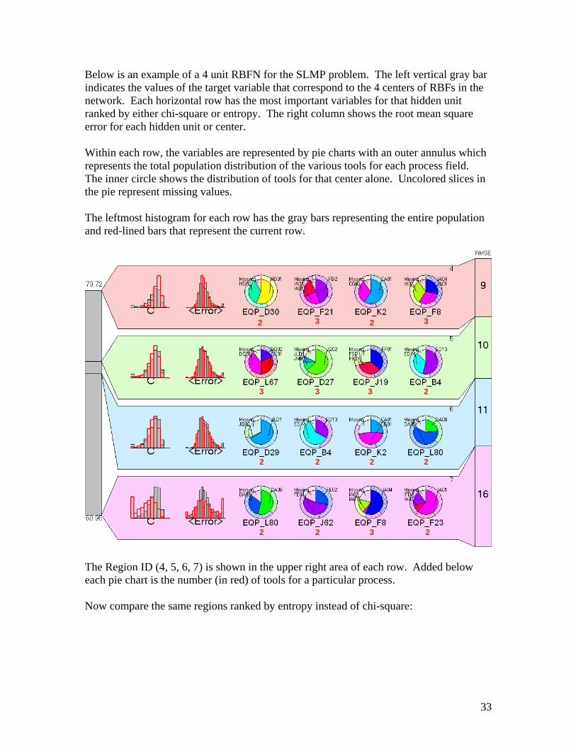
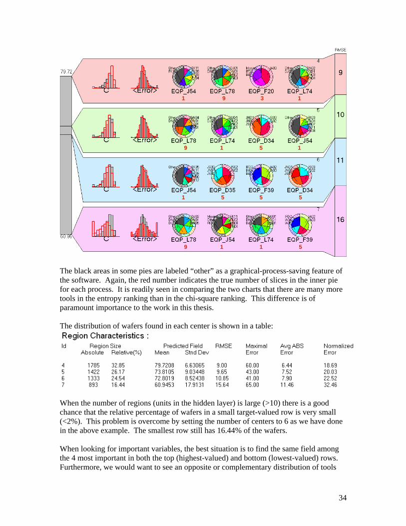
Below is an example of a 4 unit RBFN for the SLMP problem. The left vertical gray bar indicates the values of the target variable that correspond to the 4 centers of RBFs in the network. Each horizontal row has the most important variables for that hidden unit ranked by either chi-square or entropy. The right column shows the root mean square error for each hidden unit or center. Within each row, the variables are represented by pie charts with an outer annulus which represents the total population distribution of the various tools for each process field. The inner circle shows the distribution of tools for that center alone. Uncolored slices in the pie represent missing values. The leftmost histogram for each row has the gray bars representing the entire population and red-lined bars that represent the current row.

3 3

3 3

3 2 22

2 2 2 2

2

22

3

The Region ID (4, 5, 6, 7) is shown in the upper right area of each row. Added below each pie chart is the number (in red) of tools for a particular process. Now compare the same regions ranked by entropy instead of chi-square:

33

5

5 5

5 1

1

1

1 9

9

9 1

1

1

5

3

The black areas in some pies are labeled “other” as a graphical-process-saving feature of the software. Again, the red number indicates the true number of slices in the inner pie for each process. It is readily seen in comparing the two charts that there are many more tools in the entropy ranking than in the chi-square ranking. This difference is of paramount importance to the work in this thesis. The distribution of wafers found in each center is shown in a table:

When the number of regions (units in the hidden layer) is large (>10) there is a good chance that the relative percentage of wafers in a small target-valued row is very small (<2%). This problem is overcome by setting the number of centers to 6 as we have done in the above example. The smallest row still has 16.44% of the wafers. When looking for important variables, the best situation is to find the same field among the 4 most important in both the top (highest-valued) and bottom (lowest-valued) rows. Furthermore, we would want to see an opposite or complementary distribution of tools

34

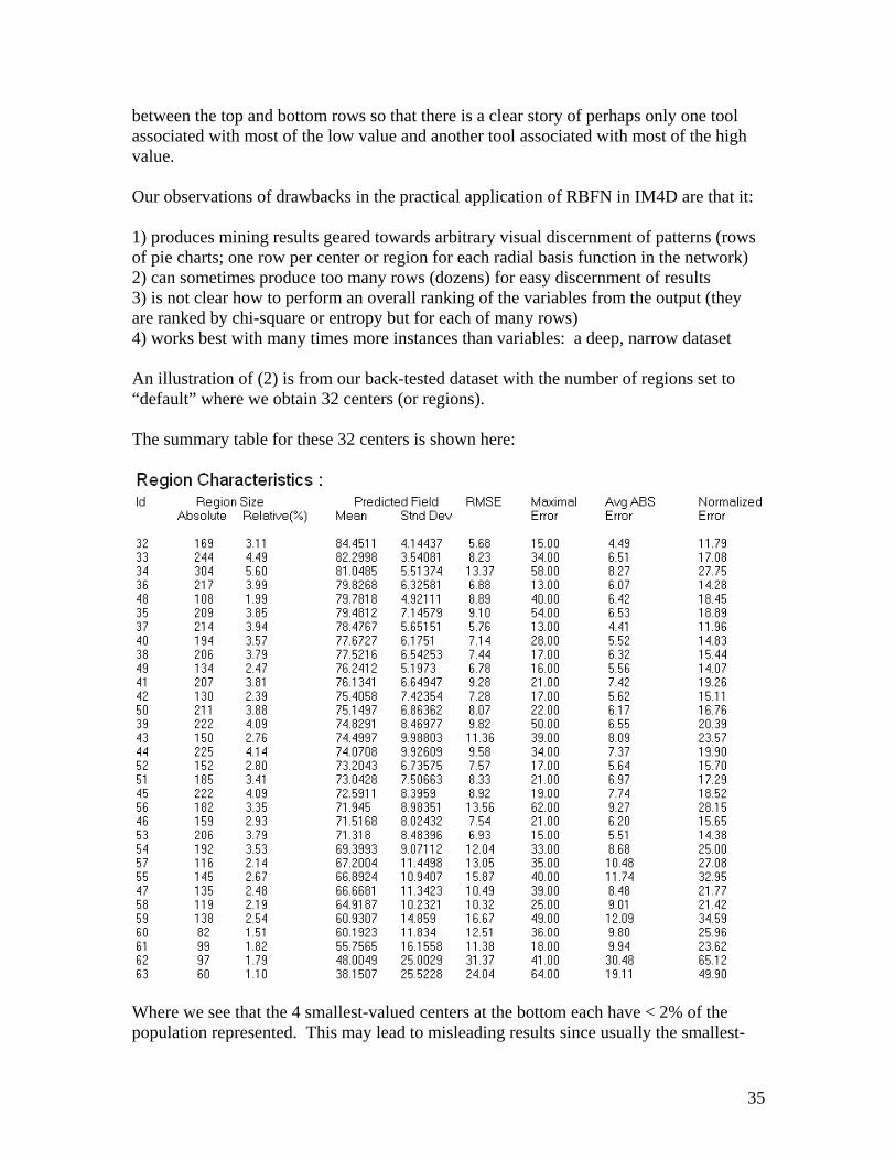
between the top and bottom rows so that there is a clear story of perhaps only one tool associated with most of the low value and another tool associated with most of the high value. Our observations of drawbacks in the practical application of RBFN in IM4D are that it: 1) produces mining results geared towards arbitrary visual discernment of patterns (rows of pie charts; one row per center or region for each radial basis function in the network) 2) can sometimes produce too many rows (dozens) for easy discernment of results 3) is not clear how to perform an overall ranking of the variables from the output (they are ranked by chi-square or entropy but for each of many rows) 4) works best with many times more instances than variables: a deep, narrow dataset An illustration of (2) is from our back-tested dataset with the number of regions set to “default” where we obtain 32 centers (or regions). The summary table for these 32 centers is shown here:

Where we see that the 4 smallest-valued centers at the bottom each have < 2% of the population represented. This may lead to misleading results since usually the smallest-

35

valued row is compared to the largest-valued row. The RMSE is also noticeably larger for these bottom rows. As mentioned above, the intuitively appealing nature of radial basis function networks is that they have features similar to both clustering and neural networks. Each ‘cluster’ is centered at an RBF region with a, typically, Gaussian ‘distance measure’ capturing points within its radius. The RBF method can use categorical or numeric input (or both) and output. The regions are found automatically by the RBF algorithm and can be adjusted in the minimum number of points defining a region as well as the quantity of regions to include in the model. If these are not specified, the software uses default values. To fine tune the RBF method for best results in this work, this sequence was used: 1) Set the number of regions to that number (typically 4 or 6) which will provide on the order of 10% of the data in the extreme (e.g. highest or lowest target values) regions of interest. Although the Redbook69 suggests finding a ratio of 2 between the regions’ highest and lowest target values (for numeric prediction) I find that the percentage of points in these regions is probably more important and that the ratio is not important. 2) Save the partition details for the highest and lowest regions as text files and load them into a spreadsheet program. 3) In the spreadsheet, rank each of the 2 regions by chi-square (provided) and create a (Pareto) chart of the variables’ target values. Include the topmost variables as features for further modeling. Alternatively, select the top 50 (depending on the total number of variables and the number the next model can accept). Our initial RBF summary table illustrated the utility of (1) when we ran the RBFN with regions=6 (resulting in 4 centers) for the same dataset as used above. We immediately notice that there are only 4 rows (regions) and the values of the target are less extreme than in the 22 region case: 0.8118—1.008 vs. 0.728—1.05. For illustrative purposes, let’s next compare between the ranking of our results for the above 32 and 4 regional RBFNs by chi-square vs. entropy. The entropy ranking contains many processes with a large number of attributes (tools). The chi-square ranking is less susceptible to this bias and snags our true causative tool. The chi-square formula used in IM4D is: 70

2

2

1

1100( 1)

i id

k

ii

c pc P

pdP

χ=

⎛ ⎞−⎜ ⎟

⎝ ⎠=− ∑

Where: k = a fixed partition

69 C. Baragoin, C. M. Andersen, S. Bayerl, G. Bent, J. Lee, C. Schommer, Mining Your Own Business in Retail: Using DB2 Intelligent Miner for Data, IBM Redbooks, August, 2001, pp.111—116, 126—130. 70 This information is (until 2008) available from IBM’s help site for IM4D.

36

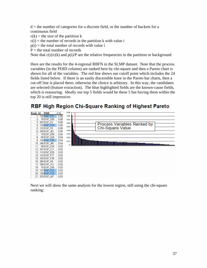
d = the number of categories for a discrete field, or the number of buckets for a continuous field c(k) = the size of the partition k c(i) = the number of records in the partition k with value i p(i) = the total number of records with value i P = the total number of records Note that c(i)/c(k) and p(i)/P are the relative frequencies in the partition or background Here are the results for the 4-regional RBFN in the SLMP dataset. Note that the process variables (in the PDID column) are ranked here by chi-square and then a Pareto chart is shown for all of the variables. The red line shows our cutoff point which includes the 24 fields listed below. If there is an easily discernible knee in the Pareto bar charts, then a cut-off line is placed there; otherwise the choice is arbitrary. In this way, the candidates are selected (feature extraction). The blue highlighted fields are the known-cause fields, which is reassuring. Ideally our top 5 fields would be these 5 but having them within the top 20 is still impressive.

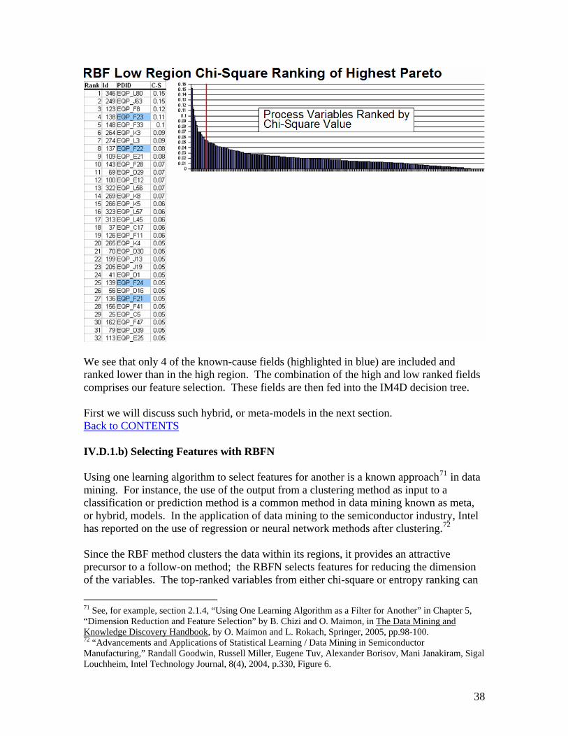
Next we will show the same analysis for the lowest region, still using the chi-square ranking:

37

We see that only 4 of the known-cause fields (highlighted in blue) are included and ranked lower than in the high region. The combination of the high and low ranked fields comprises our feature selection. These fields are then fed into the IM4D decision tree. First we will discuss such hybrid, or meta-models in the next section. Back to CONTENTS IV.D.1.b) Selecting Features with RBFN Using one learning algorithm to select features for another is a known approach71 in data mining. For instance, the use of the output from a clustering method as input to a classification or prediction method is a common method in data mining known as meta, or hybrid, models. In the application of data mining to the semiconductor industry, Intel has reported on the use of regression or neural network methods after clustering.72

Since the RBF method clusters the data within its regions, it provides an attractive precursor to a follow-on method; the RBFN selects features for reducing the dimension of the variables. The top-ranked variables from either chi-square or entropy ranking can

71 See, for example, section 2.1.4, “Using One Learning Algorithm as a Filter for Another” in Chapter 5, “Dimension Reduction and Feature Selection” by B. Chizi and O. Maimon, in The Data Mining and Knowledge Discovery Handbook, by O. Maimon and L. Rokach, Springer, 2005, pp.98-100. 72 “Advancements and Applications of Statistical Learning / Data Mining in Semiconductor Manufacturing,” Randall Goodwin, Russell Miller, Eugene Tuv, Alexander Borisov, Mani Janakiram, Sigal Louchheim, Intel Technology Journal, 8(4), 2004, p.330, Figure 6.

38

be compared for matches (e.g. visually using a Pareto chart) as a form of voting. Another possible approach is to find matches among highly chi-square ranked variables between the RBF regions for the highest and lowest target values. Next we have the problem of reconciling or accounting for results from the different regions of the RBFN. Since each region is individually ranked, it is very likely, for hundreds of variables, that a different variable will be ranked highest in each region. IM4D’s RBFN results are presented in the order of their distributions of the target variable typically with the highest-valued region as the top row of results. One can therefore look at the topmost and bottommost regions to try to find the same variable among those that are top ranked. The next consideration is whether the same tool is predominant in both regions for a variable (process). If this is the case, then it may merely indicate that a particular tool has a wide variation in its values and is both the best and worst tool according to the target values of its records (wafers). A design of experiments (using ANOVA) could then clarify from where the variation occurs and be corrected. However, we would rather find different tools, for a given process, between the top and bottom regions for a highly ranked process. In IM4D this can be done visually by comparing the pie charts to see if there is a large difference in tools (inner pie slices) compared to the overall population’s distribution in that tool (outer circle). I have found that an easier approach is to let a tree do this discrimination. We then have used the RBFN for feature selection – using its top ranked variables, followed by sequential trees to discriminate among the tools for each variable. The RBFN may require fine-tuning to determine the best number of regional centers as well as discovering the best way to use its output directly for interpretation or as input to a follow-on mining method (decision tree). Rules for single or combined equipment paths can then be obtained in view of the desired value of the electrical characteristic. Ultimately, the ranked output of each method is compared to the known cause(s) in order to find the best method. Back to CONTENTS IV.D.2) Classification and Regression Trees IV.D.2.a) Operation of the basic tree method Tree methods are very popular73 among, and a mainstay of, data miners. The data is split two or more ways at each node or branch in the tree according to which variable best separates them by one of various criteria (e.g. Gini, Information Gain, Gain ratio). An inherent drawback of this approach is that the dataset is reduced in size after each split, so the significance of such variables is pertinent only to the sub-branch which it separates. This splitting continues down to the final leaves. The variable splitting the top or initial node is the only one of interest to us here. 73 see, for example, the KDnuggets poll archive at www.kdnuggets.com

39

IV.D.2.b) Sequential top node method74

In this method of KDD using trees, after the tree is formed, the top node is

recorded and then removed and the tree method is applied again to find the 2nd-most important variable. Repeating this to completion among the variables creates a hierarchy of rules ranked by their importance. With hundreds of variables, this is performed only after a feature selection method reduces the number of variables down to a more manageable dataset.

Such a method has been used with the 1R tree “stump” method (found in WEKA) to create single node rules.75

Back to CONTENTS

IV.E) Rules for Multiple Process Tools

If a subject matter expert (SME, e.g. a manufacturing or device yield engineer) suspects that there is a process-to-process interaction between tools, such as between a lithography tool and a subsequent etching process’ tool, then it would be useful to retain 2 levels in each tree for the SME to peruse. This could be performed for each tree but the “stump” single-node tree could not be used. In IM4D, by setting the number of levels to 2, such 2-node trees are easily produced.

When a “match” to intuition or experience is made by the SME between the top and second node variables (processes) then both process variables (top and 2nd nodes) of the tree should be added to the pool of variables before proceeding with the sequential elimination of top nodes as described in the section above. Matches in this case are processes that are strongly related in the formation of a device feature that can directly or indirectly affect the electrical parameter used as the target. As mentioned, a common interaction of variables is for the definition of a feature which involves photolithographically defining the shape’s boundary features and a subsequent etching step that reproduces the photolithographically-defined pattern into an underlying film. The degree of exactness of the pattern transfer down to the base of the underlying film depends on how vertical (anisotropic) the walls of the pattern are. The process variables of the etching process can strongly affect this anisotropy. The feature dimensions at the base of the film may define the region for doping the underlying silicon comprising the active device region (e.g. the gate channel) and therefore is of paramount importance in device performance (e.g. speed of switching for gate length).

An example of a rule for multiple process tools would be:

If tools JS06, JN03, or JS05 are used at the D39 process step AND If tool IA01 is used at the F23 step

74 This method was first described to me in a private conversation with an IBM colleague, Roger Cheek. 75 Holmes, G. and Nevill-Manning, C.G., “Feature selection via the discovery of simple classification rules,” Proc. Symp. Intelligent Data Analysis, Baden-Baden, Germany, 1995. http://www.cs.waikato.ac.nz/~ml/publications/1995/Holmes95-IDA95.pdf

40

THEN C = 69.348 for 2,386 wafers (29% of the entire population) The electrical parameter is reduced in value by 5.5% from the overall mean for 29% of the wafers. The interaction of D39 with F23 may make sense to the SME. This is shown below in Node ID 1.1.1 in the tree summary from Intelligent Miner for Data.

The tree diagram provides a histogram of the target variable “C” and pie charts of the distribution of tools used at the process steps. For example, the distribution in Node Id 1.1.2 (4th row below) has a distribution (tan bars in front of background population’s gray bars) that is slightly higher than that of Node 1.1.1 (3rd row). The predominant tool used in process F23 (rightmost column) is IFD2 for node 1.1.2.

We now return to our analysis of the SLMP data where we selected features based on a 4-region RBF with chi-square ranking.

41

The decision tree is not run in the usual way, but is run as a stump where we are interested in only the top node. That field is then eliminated from the input fields and another stump is run. In this way, we have a listing of sequential top nodes: This is the 1st or top node tree stump that we obtain for the SLMP dataset with chi-square feature selection from a 4-region RBFN:

The next tree obtained is:

We continue in this manner until we have exhausted all of the selected features with as many tree stumps formed. We are then ready for our visualization approach described in the next section. Back to CONTENTS IV.E.1) Method for Summarizing and Prioritizing Rules: The Tree Curve76

A distinct disadvantage with knowledge discovery vs. predictive analytics where there are roughly as many variables as records is the lack of diagnostic methods, such as gain or lift curves, to compare mining methods. The use of the hypergeometric method mentioned in Part III.D for categorical variables is appropriate for classification problems but our target is continuous. We could bin our continuous target for classification, but often a binning boundary, or cutoff, is difficult to determine in electrical test parameters. A method introduced in this work is that of the “tree curve.” Rather than simply rank the variables again using sequential top nodes from the tree, we will plot the nodes on a chart with the number of records (wafers) vs. target value (electrical parameter). The mining results can then be judged in importance visually by the end-user. The general form of the tree curve is shown below. It has the shape of a cusp where the apex is defined by the mean of the population. Any rules obtained from the tree will involve a smaller number than the total population due to the splitting nature of nodes. Rules which result in target values less than the mean will be represented by a cloud of points roughly on or below the left curve; complementarily, those higher than the mean

76 Submitted by the author as an invention in IBM.

42

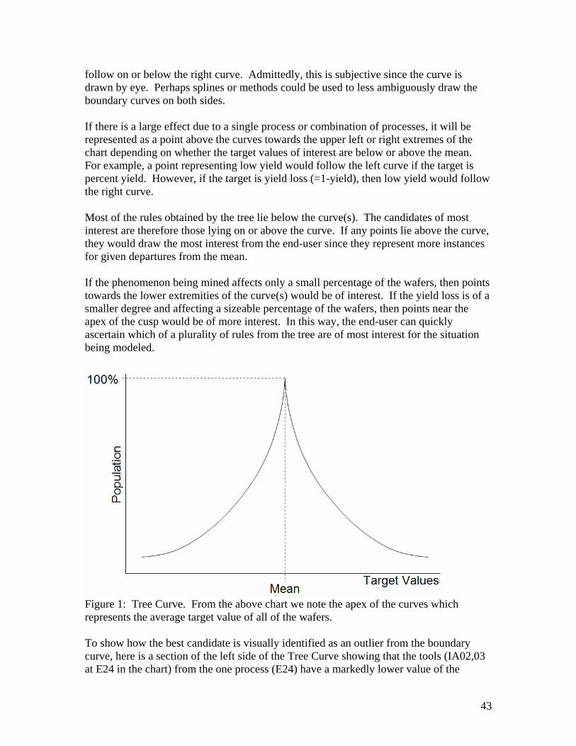
follow on or below the right curve. Admittedly, this is subjective since the curve is drawn by eye. Perhaps splines or methods could be used to less ambiguously draw the boundary curves on both sides. If there is a large effect due to a single process or combination of processes, it will be represented as a point above the curves towards the upper left or right extremes of the chart depending on whether the target values of interest are below or above the mean. For example, a point representing low yield would follow the left curve if the target is percent yield. However, if the target is yield loss (=1-yield), then low yield would follow the right curve. Most of the rules obtained by the tree lie below the curve(s). The candidates of most interest are therefore those lying on or above the curve. If any points lie above the curve, they would draw the most interest from the end-user since they represent more instances for given departures from the mean. If the phenomenon being mined affects only a small percentage of the wafers, then points towards the lower extremities of the curve(s) would be of interest. If the yield loss is of a smaller degree and affecting a sizeable percentage of the wafers, then points near the apex of the cusp would be of more interest. In this way, the end-user can quickly ascertain which of a plurality of rules from the tree are of most interest for the situation being modeled.

Figure 1: Tree Curve. From the above chart we note the apex of the curves which represents the average target value of all of the wafers. To show how the best candidate is visually identified as an outlier from the boundary curve, here is a section of the left side of the Tree Curve showing that the tools (IA02,03 at E24 in the chart) from the one process (E24) have a markedly lower value of the

43

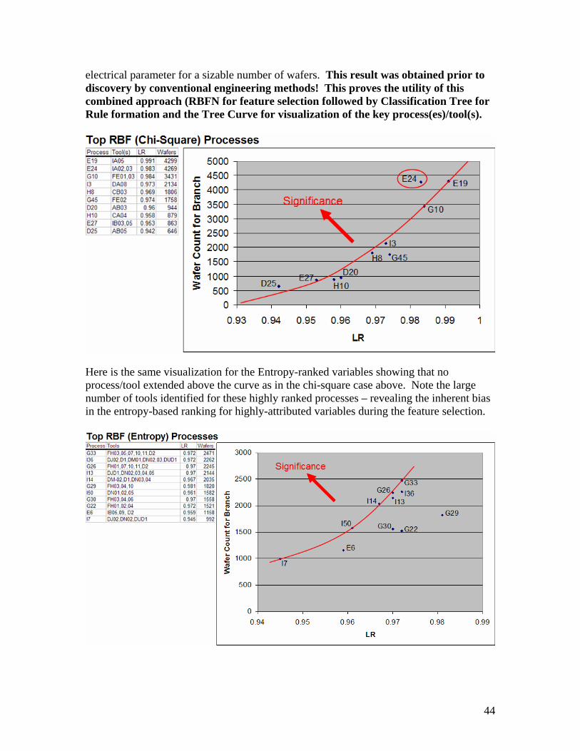
electrical parameter for a sizable number of wafers. This result was obtained prior to discovery by conventional engineering methods! This proves the utility of this combined approach (RBFN for feature selection followed by Classification Tree for Rule formation and the Tree Curve for visualization of the key process(es)/tool(s).

Here is the same visualization for the Entropy-ranked variables showing that no process/tool extended above the curve as in the chi-square case above. Note the large number of tools identified for these highly ranked processes – revealing the inherent bias in the entropy-based ranking for highly-attributed variables during the feature selection.

44

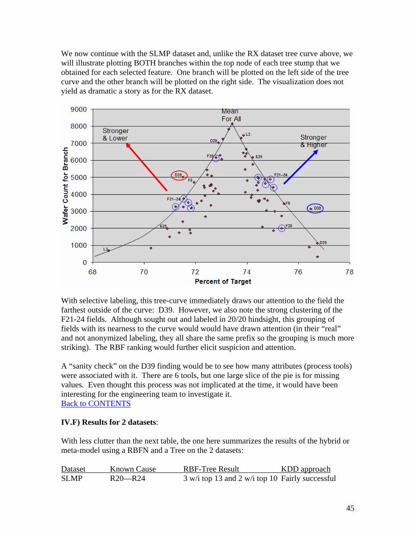
We now continue with the SLMP dataset and, unlike the RX dataset tree curve above, we will illustrate plotting BOTH branches within the top node of each tree stump that we obtained for each selected feature. One branch will be plotted on the left side of the tree curve and the other branch will be plotted on the right side. The visualization does not yield as dramatic a story as for the RX dataset.

With selective labeling, this tree-curve immediately draws our attention to the field the farthest outside of the curve: D39. However, we also note the strong clustering of the F21-24 fields. Although sought out and labeled in 20/20 hindsight, this grouping of fields with its nearness to the curve would would have drawn attention (in their “real” and not anonymized labeling, they all share the same prefix so the grouping is much more striking). The RBF ranking would further elicit suspicion and attention. A “sanity check” on the D39 finding would be to see how many attributes (process tools) were associated with it. There are 6 tools, but one large slice of the pie is for missing values. Even thought this process was not implicated at the time, it would have been interesting for the engineering team to investigate it. Back to CONTENTS IV.F) Results for 2 datasets: With less clutter than the next table, the one here summarizes the results of the hybrid or meta-model using a RBFN and a Tree on the 2 datasets: Dataset Known Cause RBF-Tree Result KDD approach SLMP R20—R24 3 w/i top 13 and 2 w/i top 10 Fairly successful

45

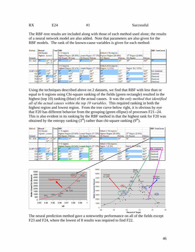
RX E24 #1 Successful The RBF-tree results are included along with those of each method used alone; the results of a neural network model are also added. Note that parameters are also given for the RBF models. The rank of the known-cause variables is given for each method:

Using the techniques described above on 2 datasets, we find that RBF with less than or equal to 6 regions using Chi-square ranking of the fields (green rectangle) resulted in the highest (top 10) ranking (blue) of the actual causes. It was the only method that identified all of the actual causes within the top 10 variables. This required ranking in both the highest region and lowest region. From the tree curve below right, it is obvious by eye that F20 has different behavior from the grouping (green ellipse) of processes F21--24. This is also evident in its ranking by the RBF method in that the highest rank for F20 was obtained by the entropy ranking (3rd) rather than chi-square ranking (9th).

The neural prediction method gave a noteworthy performance on all of the fields except F23 and F24, where the lowest of 8 results was required to find F22.

46

The decision tree method alone was poor across the board. Its lack of performance was a strong motivator for embarking on this entire work. The RBF-TreeCurve method mirrored the RBF, Chi-square methods for the RX dataset. However, it was not as strong in identifying the causes for the SLMP dataset other than the fact that F21-24 were clustered tightly together and slightly penetrated the curve. A key qualification for success in the SLMP dataset was to obtain enough F20-F24 fields in a high ranking so that suspicion would be directed towards a process tool that was common to all of these F steps. By that criterion, the tree-curve is a success since the tight clustering of F21-24 would immediately raise the question to the observer as to the cause of their joint behavior. This further justifies the thrust of the work in this thesis. In summary, this work introduces the use of a RBFN to select variables which are used as the input to a sequential tree (with 1 or 2 levels) finding top nodes that are then plotted in a tree-curve to allow a visual confirmation of highly-ranked candidates associated with the mining target. Back to CONTENTS V. Further Study V.A) Mining Methods As described above, the QUEST tree method is touted as being unbiased towards multi-attributed variables which is one of the major problems encountered in mining semiconductor manufacturing logistics data. The QUEST tree or any tree using the MDL method for node splitting would be logical next steps beyond this work. Since SVMs were noted by some authors to be superior to RBFNs it would be interesting to use a SVM with a RBF kernel and compare the results for feature selection. IM4D does not offer SVM mining. V.B) Feature Creation A promising avenue of study77 would be to transform the logistics dataset so that similar processes with identical tools are reduced to a single variable. A common objection to being asked to investigate a data mining result by the process engineering team is if there are similar processes to the result and which use the same tool as the result but which have no signal or indication of being a problem. “If the tool is bad for process A then why isn’t it bad for process B?” This question is especially valid when process B is a repetition of process A during the formation of a repetitive structure such as when forming different levels of metal interconnect lines. Unless it can be shown that a layout design ground rule is violated at a particular level so that it is more susceptible to a short or misalignment, it is difficult to obtain “buy-in” from the process engineers or their management that the mining result is real. 77 Disclosed by the author as an invention within IBM on December 18, 2006.

47

If such similar processes are combined into a single variable, and it is ranked highly in the mining results, then the objection is less likely to occur. Such a transformation is likely to make the signal stronger and easier to find by the mining method. The alternative is to hope that the signal is equally strong among the similar processes so that all of them are highly ranked. A private observation by the author is that not all mining methods are equal to this task and a favorite mining method may easily miss such a combined signal. The determination of which processes should be combined into single variables could be easily made by subject matter experts, specifically process integration teams. Please note that such a transformed dataset should be mined separately from the original dataset since the possibility of a problem at a particular level, not due to a common tool among similar levels, is still real. V.C) Dataset Access Limitations Due to Commercial Prudence Typical of applied data mining studies is the proprietary nature of the algorithms used in the data mining method as well as the dataset. However, for those mining manufacturing data in industry, the generic description of the method and the availability of manufacturing data should suffice not only in the testing of the findings from this study but also as a springboard to the testing of new or comparable mining methods. Since this study involves manufacturing data from a company in a highly competitive industry, the dataset is proprietary. This prevents the testing of alternative methods on this dataset unless performed by those from this company. This is a common situation in the mining literature involving semiconductor manufacturing. [1-12] Unfortunately, this limits research of these problems to those within, or funded by, this industry. Back to CONTENTS Appendix A: Acronyms for Process Variables AERO for cryogenic aerosol cleaning CMP for chemical mechanical planarization CVD for chemical vapor deposition FRN for furnace INS for insulator ION for ion implantation LNR for liner LTH for photolithography MTL for metal PE for plasma activated PLT for plating RIE for dry, or reactive ion, etching RTP for rapid thermal processing

48

WET for wet chemical etching or cleaning Acronyms AMD = Advanced Micro Devices ANOVA for analysis of variance APC for advanced process control CART for classification and regression tree CCDF for complementary CDF CDF for cumulative distribution function CRM for customer relationship management CSV for comma separated variables DoE for design of experiments GHz for gigaHerz (10E6 cycles/sec) GUI = graphical user interface ILT for in-line electrical test IM4D = intelligent miner for data KDD for knowledge discovery in data MDL for minimum description length PDID for process description identification PNN for probabilistic neural network QUEST for quick unbiased efficient statistical tree R&D for research and development RBF = radial basis function network RBFN = RBF network ROC for receiver operator characteristic ROI = return on investment SME = subject matter expert SPC for statistical process control TSMC (Taiwan Semiconductor Manufacturing Company Back to CONTENTS Appendix B: Cited Books 1) Dhammika Amaratunga and Javier Cabrera, Exploration and Analysis of DNA Microarray and Protein Array Data, Wiley Series in Probability and Statistics, 2004. 2) C. Baragoin, C. M. Andersen, S. Bayerl, G. Bent, J. Lee, C. Schommer, Mining Your Own Business in Retail: Using DB2 Intelligent Miner for Data, IBM Redbooks, August, 2001. 3) Christopher M. Bishop, Neural Networks for Pattern Recognition, Oxford, 1995 4) Peter Cabena, Pablo Hadjinian, Rolf Stadler, Jaap Verhees & Alessandro Zanasi, Discovering Data Mining From Concept To Implementation, , Prentice Hall, 1998. 5) C.H. Chen, ed., Fuzzy Logic and Neural Network Handbook, IEEE Press, 1996

49

6) Nello Cristianini and John Shawe-Taylor, An Introduction to Support Vector Machines and other Kernel-based Learning Methods, Cambridge, 2000

7) Margaret H. Dunham, Data Mining: Introductory and Advanced Topics, , Prentice Hall, 2003. 8) Jiawei Han and Micheline Kamber, Data Mining: Concepts and Techniques, 2nd edn., Morgan Kaufmann, 2006. 9) Trevor Hastie, Robert Tibshirani and Jerome Friedman, The Elements of Statistical Learning: Data Mining, Inference and Prediction, Springer, 2001. 10) Simon Haykin, Neural Networks: A Comprehensive Foundation, IEEE Press, 1994 11) Robert V. Hogg and Elliot A. Tanis, Probability and Statistical Inference, 6th edn., , Prentice Hall, 2001. 12) IBM DB2 Intelligent Miner for Data: Using the Intelligent Miner for Data, Version 6, Release 1, IBM, 1999. 13) Mehmed Kantardzic, Data Mining: Concepts, Models, Methods, and Algorithms, Wiley Interscience, 2003. 14) Daniel T. Larose, Discovering Knowledge in Data: An Introduction to Data Mining, Wiley, 2005. 15) Daniel T. Larose, Data Mining Methods and Models, Wiley, 2006 16) Oded Maimon and Lior Rokach, eds., The Data Mining and Knowledge Discovery Handbook, Springer, 2005. 17) Thomas Mitchell, Machine Learning, McGraw-Hill, 1997. 18) Douglas C. Montgomery, Design and Analysis of Experiments, 6th edn., Wiley Press, 2005. 19) Dorian Pyle, Data Preparation for Data Mining, Morgan Kaufman, 1999. 20) Dorian Pyle, Business Modeling and Data Mining, Morgan Kaufmann, 2003. 21) Bernhard Scholkopf and Alexander J. Smola, Learning with Kernels: SVMs, Regularization, Optimization, and Beyond, MIT Press, 2002. 22) Lipo Wang and Xiuju Fu, Data Mining with Computational Intelligence, Springer, 2005.

50

23) Ian Witten and Eibe Frank, Data Mining: Practical Machine Learning Tools and Techniques, 2nd edn, Elsevier, 2005 24) S. Wolf and R. Tauber, Silicon Processing for the VLSI Era, Vol. 1: Process Technology, 2nd edn., Lattice Press, 1999. Back to CONTENTS Biography of the Author Steven G. Barbee is continuing his second career in data mining as a Sales Engineer with SPSS, Inc. He retired from IBM after having mined semiconductor manufacturing data for 4 years as a Senior Engineer in IBM's Systems and Technology Group in East Fishkill, NY. Prior to that he was a Senior Engineering Manager in IBM's Microelectronics Division reporting to the Research Division where he supervised the R & D of specific semiconductor unit processes and their control. He is a patentee (33 US patents) and author in this field. He served as a National Science Foundation Auditor for the two annual reviews of the Engineering Research Center at North Carolina State University. He holds a Master of Science degree concentrated in plasma physics from Columbia University's School of Engineering and Applied Science. He earned a Bachelor of Arts degree in Physics and Math, summa cum laude, from Doane College. He is a member of the IEEE Computer Society, the American Computer Society and the New York Academy of Sciences and a past member of the American Physical Society and the American Vacuum Society. His community interests include leading an alpha class as a deacon at the Warren Congregational Church in Connecticut; prior to that he served as senior warden and licensed lay reader of an Episcopal church. He held two national staff positions at the ’93 and ‘97 National BSA Jamborees and served his local community as Scoutmaster for 9 years. Mr. Barbee is married with two sons (Paul and David); his extended family includes 4 international exchange student “sons” (Rob, Minh, Ashley and Tercio). He resides with his wife, Debbie, in Amenia, New York.

51