The Domestic and International Effects ofFinancial Deregulation

Fabio Ghironi∗

Boston College,

EABCN, and NBER

Viktors Stebunovs†

Boston College

July 20, 2007

Preliminary

Comments Welcome

Abstract

This paper studies the domestic and international effects of financial deregulation in a dynamic,

stochastic, general equilibrium model with endogenous producer entry. We model deregulation as

a decrease in the monopoly power of financial intermediaries. We show that the economy that

deregulates experiences an increase in size, real exchange rate appreciation, and a persistent current

account deficit. The rest of the world experiences higher consumption and an expansion in the

number of domestic producers. Less monopoly power in financial intermediation results in less volatile

business creation, reduced markup countercyclicality, and weaker substitution effects in labor supply

in response to productivity shocks. Financial deregulation thus contributes to a moderation of firm-

level and aggregate output volatility. In turn, trade and financial ties between the two countries allow

the foreign economy to enjoy lower volatility as well. The results of the model are consistent with

features of U.S. and international data following the U.S. banking deregulation started in 1977.

1 Introduction

The 1980s and late 1990s were characterized by real appreciation of the U.S. dollar and persistent U.S.

current account deficits. The decades after the early 1980s were also marked by a reduction of macroeco-∗Department of Economics, Boston College, 140 Commonwealth Avenue, Chestnut Hill, MA 02467-3859, U.S.A. or

Fabio.Ghironi@bc.edu. URL: http://www2.bc.edu/~ghironi.†Department of Economics, Boston College, 140 Commonwealth Avenue, Chestnut Hill, MA 02467-3859, U.S.A. or

stebunov@bc.edu. URL: http://www2.bc.edu/~stebunov.

1

nomic volatility around the world. This paper develops a model of the domestic and international effects

of financial deregulation to study the contribution to these phenomena of the U.S. banking deregulation

started in 1977 and finalized in 1994.

Our model builds on Ghironi and Melitz (2005), Bilbiie et al (2005), and Stebunovs (2006) by in-

corporating endogenous producer entry subject to sunk costs, deviations from purchasing power parity

(PPP), and a role for financial intermediation. Investment in the model takes the form of the creation of

new production lines (for convenience, identified with firms). Sunk costs and a time-to-build lag induce

the number of firms (producers, production lines) to respond slowly to shocks, consistent with the notion

that the number of productive units is fixed in the short run.1 Following Stebunovs (2006), we assume

that new entrants must obtain funds from financial intermediaries (henceforth, banks) to cover entry

costs. Banks with market power erect a financial barrier to firm entry to protect the profitability of

existing borrowers, reducing average entry relative to the competitive benchmark of Bilbiie et al (2005).2

We take bank concentration as exogenous to the business cycle, and we interpret financial deregulation

as an exogenous decrease in bank monopoly power.

We show that the economy that deregulates experiences an increase in size, real exchange rate ap-

preciation, and a persistent current account deficit. Bank deregulation makes the domestic economy a

relatively more attractive environment for potential entrants in the presence of trade costs. As in Ghironi

and Melitz (2005), entry in the domestic economy pushes relative labor costs upward, inducing real appre-

ciation when the economy features a non-traded sector or home bias in preferences. When economies are

allowed to borrow and lend, financial deregulation induces the home economy to run persistent current

account deficits to finance increased firm entry. The rest of the world experiences higher consumption

and an expansion in the number of domestic producers. In addition, less monopoly power in financial

intermediation results in less volatile business creation, reduced markup countercyclicality, and weaker

substitution effects in labor supply in response to productivity shocks — the source of business cycles in

our model. Financial deregulation thus contributes to a moderation of firm-level and aggregate output

volatility. In turn, trade and financial ties between the two countries allow the foreign economy to enjoy

lower volatility as well. Interpreting the economy that deregulates its financial sector as the U.S., the

predictions of our model are thus consistent with features of the empirical evidence following the U.S.1This is in contrast to other recent contributions, such as Comin and Gertler (2006) and Jaimovich (2006), whose entry

mechanisms allow instantaneous variation in the number of producing firms.2The model thus incorporates Cestone and White’s (2003) insight that entry deterrence takes place through financial

rather than product markets, and it explains the empirical evidence in Cetorelli and Strahan (2006).

2

banking deregulation started at the end of the 1970s.3

Our paper contributes to several literatures that address observed dynamics of international relative

prices, external imbalances, and the moderation of business cycle volatility observed since the mid 1980s.

The conventional explanation for the contemporaneous occurrence of exchange rate appreciation and

external borrowing in the U.S. in the 1980s relied on the traditional Mundell-Fleming analysis of the

consequences of expansion in government spending. But the tight association between federal budget

and external balance has been challenged by recent literature. For instance, Erceg et al (2005) find that a

fiscal deficit has a relatively small effect on the U.S. trade balance, irrespective of whether the source is a

spending increase or tax cut. With respect to U.S. trade balance and real exchange rate dynamics in the

second half of the 1990s, Hunt and Rebucci (2005) conclude that accelerating productivity growth in the

U.S. contributed only partly to the appreciation and the trade balance deterioration. They find that a

portfolio preference shift in favour of U.S. assets and some uncertainty and learning about the persistence

of both shocks are needed for their model to explain the data. Rather than emphasizing the demand-side

effect of preference shifts, Caballero et al (2006) provide a model that rationalizes persistent imbalances

as the outcome of potential growth differentials among different regions of the world and heterogeneity

in these regions’ capacity to generate financial assets.4 Mendoza et al (2007) argue that imbalances can

be the outcome of international financial integration when countries differ in financial market deepness

(interpreted as the enforcement of financial contracts) and show that countries with more advanced

financial markets accumulate foreign liabilities in a gradual, long-lasting process. Finally, Fogli and Perri

(2006) argue that global imbalances are a natural consequence of business cycle moderation in the U.S.

In their model, if a country experiences a fall in volatility greater than that of its partners, its relative

incentives to accumulate precautionary savings weaken, and this results in an equilibrium permanent

deterioration of its external balance.5

Our model provides an alternative, potentially complementary explanation of observed phenomena,

based on the effects of deregulation that made the U.S. banking system more competitive than that of the

rest of the world. De Bandt and Davis (2000) provide evidence that the behavior of large banks in Europe

was not as competitive as that of U.S. counterparts over the period 1992-1996. Regarding small banks, the

level of competition in Europe was even lower. In our model, a differential in the competitiveness of the3Our model also implies that deregulation is welfare improving in both countries as households enjoy higher utility from

consumption despite an increase in labor supply.4 See also Caballero (2006).5Other explanations emphasize demographics, a ‘global saving glut,’ and valuation effects.

3

banking system induces real appreciation of the dollar and U.S. external borrowing by making the U.S. a

more attractive environment for business creation. As in the above mentioned papers, persistent external

imbalances arise as an equilibrium phenomenon. However, while Caballero et al (2006) do not link business

cycle moderation with global imbalances, and Fogli and Perri (2006) take moderation as exogenous, we

provide a unified explanation of imbalances and moderation for given stochastic productivity process

without requiring long-run productivity differentials. An element of similarity between our approach and

those of Caballero et al (2006) and Mendoza et al (2007) is that imbalances arise as a consequence of

capital mobility across asymmetric financial systems: In Caballero et al, there is asymmetric ability to

generate financial assets; in Mendoza et al, there is asymmetric enforcement of financial contracts; in our

model, there is asymmetric banking competition.6

The remainder of the paper is organized as follows. Section 2 presents the benchmark model with

balanced trade to highlight the mechanism for real exchange rate appreciation as the result of financial

deregulation. Section 3 extends the model to allow for international capital flows to show the emergence of

external borrowing in response to deregulation. Section 4 incorporates countercyclical firm markups and

elastic labor supply to highlight the mechanism for the moderation of business cycle volatility. Finally,

Section 5 concludes. Technical details are in the Appendix.

2 Benchmark model

We begin by developing a version of our model under financial autarky.

The world consists of two countries, home (the US) and foreign (the rest of the world). We denote

foreign variables by an asterisk. Each country is populated by a unit mass of atomistic households, a

number of banks and a varying mass (number) of firms. There are several exogenously given locations

with a number of banks and a mass (number) of firms at each of them in each country.7 Each firm

is monopolistic, produces one consumption variety, competes in a domestic market and exports, has6By focusing on the role of financial intermediaries, our paper also contributes to a recent, fast growing literature on

the consequences of endogenous producer entry in macroeconomic models. In addition to the works mentioned above, seeBergin and Corsetti (2005), Bilbiie et al (2008), Corsetti, Martin, and Pesenti (2007a,b), Elkhoury and Mancini Griffoli(2006), Ghironi and Melitz (2007), Méjean (2007), and Lewis (2006). Our setup preserves the key international relativeprice and external balance implications of entry in the Ghironi-Melitz model while removing firm heterogeneity and fixedexport costs as a source of endogenous non-tradedness and introducing an exogenous non-traded sector (as in Méjean, 2007)or home bias in preferences. For simplicity, we do not allow for foreign bank ownership and foreign bank lending to domesticentrants. Intuitively, allowing for international financial integration along these dimensions will reinforce our results as itwill further undermine bank monopoly power in each country.

7 In the model the boundaries of product markets and lending markets coincide. However, in reality some larger firmsmay span multiple banking markets. In such cases, a bank could still have an impact on entry within its area of influence.

4

no collateral to pledge except a stream of future profits, and its entry is subject to a sunk entry cost.

Unspecified financial frictions force a prospective entrant to borrow the amount necessary to cover the

sunk entry cost from a local bank rather than to raise funds directly in an equity market. Borrowing

at a different location is prohibited altogether. Firm entry reduces the stream of future profits of both

incumbents and entrants and thus the amount pledgeable for entry loan repayments.

Each bank, being a local monopolist, is able to extract all the future profits from a prospective entrant,

holds a portfolio of firms and decides on the number of loans to be issued (that is, on the number of

entrants).8 Each bank trades the increase in revenue from expanding its firm portfolio (portfolio expansion

effect) against the decrease in revenue from all firms in its portfolio due to stronger firm competition (profit

destruction effect). The profit destruction effect gives rise to credit rationing on the extensive margin as

not all of the prospective entrants will be funded. Thus, there is an intrinsic inefficiency built into the

model due to the presence of monopolistic banks.9 Each bank supplies one-period deposits to domestic

households in a perfectly competitive market. The bank then uses the deposits to fund firm entry. Thus,

the cost that each bank faces is the deposit interest rate.

We now focus on the home economy. Since the completion of financial deregulation in the US in 1994,

it becomes increasingly less plausible to view banking markets as local. Banks’ ability to expand across

local markets and new technologies, that allow banks to lend to distant borrowers, limited incumbent

banks’ local monopoly power.10 Consequently, we model bank deregulation as lifting the restriction on

borrowing from a bank at a different location. The number of banks in the economy might stay the

same or decrease. However, the number of banks represented locally increases, hence reducing monopoly

power.

We assume that the rest of world does not deregulate, hence monopoly power of its banks stays the

same.

For expositional simplicity, we present each economy with one location only.

All contracts and prices in the world economy are written in nominal terms. Prices are flexible. Thus,8Banks compete in the number of entrants in Cournot fashion as in the static partial equilibrium model of Gonzalez-

Maestre and Granero (2003).9 If one interprets the number of firms as the number of production lines in the economy, then a bank might be thought as

of a multi-production line company that produces a set of goods that compete within this set and also with goods producedby other multi-production line companies. Then each multi-production line company internalizes only its own ”productcannibalization.”10Black and Strahan (2002) argue that after deregulation, the effects of concentration ought to have been mitigated by

the threat of entry. That is, banking concentration no longer signals market power when barriers to entry from regulationshave been eliminated. And, in fact, they find that the effect of concentration on the rate of creation of new incorporationsdoes fall significantly with deregulation.

5

we only solve for the real variables in the model. However, as the composition of consumption baskets in

the two countries changes over time (affecting the definitions of the consumption-based price indexes), we

introduce money as a convenient unit of account for contracts. Money plays no other role in the economy.

For this reason, we do not model the demand for cash currency, and resort to a cashless economy as in

Woodford (2003).

2.1 Households

The representative home household supplies l units of labor inelastically in each period at the nominal

wage rate Wt, denominated in units of home currency. The household maximizes expected intertemporal

utility from consumption (C), EtP∞

s=t βs−t C1−γ

s

1−γ , where β ∈ (0, 1) is the subjective discount factor andγ > 0 is the inverse of the intertemporal elasticity of substitution, subject to a budget constraint. At time

t, the household consumes the basket of goods Ct. We consider two definitions of the basket of goods Ct,

both such that the purchasing power parity does not hold.

The first definition of the consumption basket distinguishes between tradeable and non-tradeable

goods. We define the basket over a set of tradeable home and foreign goods and non-tradeable good

as Ct = (CT,t/α)α (CN,t/1− α)1−α, where CT,t is the basket of tradeable goods, CN,t is the amount of

non-tradeable good, and α ∈ (0, 1) is the weight of tradeable goods in the basket. The consumption-based price index for the home economy is then Pt = (PT,t)

α(PN,t)

1−α, where PT,t is the price in-

dex of the basket of tradeable goods and PN,t is the price of non-tradeable good. At any given time

t, only a subset of goods Ωt ⊂ Ω is available at home and abroad. Hence, we define the basket of

tradeable goods as CT,t =³R

ω∈Ωt (ct(ω))(θ−1)/θ´θ/(θ−1), where θ > 1 is the symmetric elasticity of

substitution across goods. Let pt(ω) denote the home currency price of tradeable good ω, ω ⊂ Ωt,then PT,t =

³Rω∈Ωt (pt(ω))

1−θdω´1/(1−θ)

. The household’s demand for each individual tradeable good

ω is ct = α (pt (ω) /PT,t)−θPt/PT,tCt. The household’s demand for the single non-tradeable good is

CN,t = (1− α)Pt/PN,tCt.

The second definition of the consumption basket does not distinguish between tradeable and non-

tradeable goods, instead it introduces home bias in consumption. We define the basket over a set

of home and foreign goods as Ct =³α1/θ (cD,t)

(θ−1)/θ + (1− α)1/θ (cX,t)(θ−1)/θ´θ/(θ−1), where cD,t is

the basket of goods produced at home goods and cX,t is the basket of goods produced abroad, and

α > 0.5 is the weight of home goods in the basket, it captures home bias in consumption. Hence,

6

even though the law of one price holds in the absence of trade costs, the purchasing power parity will

not. The baskets of home and foreign goods are defined as cD,t =µZ

ω∈ΩcD,t(ω)

(θ−1)/θdω¶θ/(θ−1)

and

cX,t =

µZω∗∈Ω

cX,t(ω∗)(θ−1)/θdω∗

¶θ/(θ−1), where θ > 1 is the symmetric elasticity of substitution

across goods. At any given time t, only a subset of goods Ωt ⊂ Ω is available. Let PD,t and P ∗X,t

denote the home currency price indices of home and foreign baskets. We assume that export prices

are denominated in the currency of the export market. The consumption-based price index for the

home economy is then Pt =³α (PD,t)

θ−1+ (1− α)

¡P ∗X,t

¢θ−1´1/(1−θ). Let pD,t(ω) and p∗X,t(ω

∗) de-

note the home currency price of home and foreign goods respectively, ω ⊂ Ωt and ω∗ ⊂ Ωt, thenPD,t =

³Rω∈Ωt pD,t(ω)

1−θdω´1/(1−θ)

and P ∗X,t =³R

ω∗∈Ωt p∗X,t(ω

∗)1−θdω∗´1/(1−θ)

. The household’s de-

mand for each individual home good ω is cD,t(ω) = α (pD,t(ω)/Pt)−θ Ct and for each individual foreign

good ω∗ is cX,t(ω∗) = (1− α)¡p∗X,t(ω

∗)/Pt¢−θ

Ct.

The foreign household supplies l∗ units of labor inelastically in each period in the foreign labor market

at the nominal wage rate W ∗, denominated in units of foreign currency. It maximizes a similar utility

function, with identical parameters and similarly defined consumption baskets. The subset of goods

available for consumption in the foreign economy during period t is Ω∗t ⊂ Ω and is identical to the subsetof goods that are available in the home economy.

Households in each country hold two types of assets: shares in a mutual fund of H domestic banks and

one-period deposits supplied by domestic banks. We assume that deposits pay risk-free, consumption-

based real returns. We now focus on the home economy. Let st be the share in the mutual fund of home

banks held by the representative home household entering period t. The mutual fund pays a total profit

in each period (in units of currency) equal to the total profit of all home banks, PtP

i∈H πt(i), where

πt(i) denotes the profit of home bank i. During period t, the household buys st+1 shares in the mutual

fund. The date t price in units of currency of a claim to the future profit stream of the mutual fund is

equal to the nominal price of claims to future profits of home banks, PtPi∈H vt(i), where vt(i) is the

price of claims to future profits of bank i. The household enters period t with deposits Bt−1 in units of

consumption and mutual fund share holdings st. It receives gross interest income on deposits, dividend

income on mutual fund share holdings and the value of selling its initial share position, and labor income.

The household allocates these resources between purchases of deposits and shares to be carried into next

period and consumption. The period budget constraint (in units of consumption) is

7

Bt + stXi∈H

vt(i) + Ct = (1 + rt−1)Bt−1 + st−1Xi∈H

(πt(i) + vt(i)) + wtl, (1)

where rt−1 is the consumption-based interest rate on holdings of deposits between t − 1 and t (knownwith certainty as of t−1), and wt =Wt/Pt is the real wage. We assume that nominal returns are indexed

to inflation in the home economy, so that the deposits provide a risk-free, real return in units of home’s

consumption basket. The home household maximizes its expected intertemporal utility subject to (1).

The Euler equations for deposits and share holdings are: 1 = β(1 + rt)Et

h(Ct+1/Ct)

−γi , and vt =βEt

h(Ct+1/Ct)

−γ (πt+1 + vt+1)i, where vt =

Pi∈H vt(i) and πt+1 =

Pi∈H πt+1(i). Forward iteration of

the Euler equation for shares holdings and absence of speculative bubbles yield the value of the mutual

fund, vt, in terms of a stream of bank profits, πt∞t .

2.2 Firms

The following applies to both the economy with tradeable and non-tradeable goods and the economy

with tradeable goods only and home bias in consumption. There is a continuum of firms in each country,

each producing a different tradeable variety ω ∈ Ω. Aggregate labor productivity is indexed by Zt (Z∗t ),which represents the effectiveness of one unit of home (foreign) labor. Production requires only one

factor, labor: yt(ω) = Ztlt(ω). Firms are homogeneous as they produce with the same technology, hence

identical production cost. This cost, measured in units of the consumption good Ct, is wt/Zt. Similarly,

for foreign firms the unit cost (measured in units of the foreign consumption good) is w∗t /Z∗t , where

w∗t = W ∗t /P ∗t is the real wage of foreign workers. Home and foreign firms serve both their domestic

market as well as the export market. Exporting is costly, and involves a melting-iceberg trade cost τ > 1

(τ∗ > 1), so that for every unit of home (foreign) good shipped abroad, a fraction τ − 1 (τ∗− 1) does notarrive at the foreign (home) shore.

We now consider the home firms in the economy with both tradeable and non-tradeable goods. All

firms producing tradeable goods face a residual demand curve with constant elasticity θ in both markets,

and they set flexible prices that reflect the same proportional markup µ = θ/(θ−1) over marginal cost. LetpD,t(ω) and pX,t(ω) denote the nominal domestic and export prices of a home firm. Prices, in real terms

relative to the price index in the destination market, are then given by ρD,tρT,t = pD,t(ω)/PT,tPT,t/Pt =

µwt/Zt and ρX,tρ∗T,t = pX,t(ω)/P

∗T,tP

∗T,t/P

∗t = τQ−1t µwt/Zt, where Qt = εtP

∗t /Pt is the consumption-

8

based real exchange rate (units of home consumption per unit of foreign consumption; εt is the nominal

exchange rate, units of home currency per unit of foreign). A firm decomposes its total profit into two

portions earned from domestic sales dD,t(ω) (d∗D,t(ω)) and from export sales dX,t(ω) (d∗X,t(ω)). All these

profit levels are expressed in real terms in units of the consumption basket in the firm’s location. In the

case of a home firm, total profits in period t are given by dt(ω) = dD,t(ω) + dX,t(ω), where dD,t(ω) =

α/θ¡ρD,t

¢1−θCt and dX,t(ω) = α/θQt

¡ρX,t

¢1−θC∗t . Since all firms are identical in equilibrium, one

may drop indexing by ω. There is also a (fixed) mass of firms in each country producing the identical

non-tradeable good. These firms are perfectly competitive and possess the same technology as the firms

producing tradeable goods. Hence, the price of the non-tradeable good, in real terms relative to the

domestic price index, is given by ρN,t = PN,t/Pt = wt/Zt. Foreign firms behave in a similar way.11

We now consider the home firms in the economy with tradeable goods only and home bias in con-

sumption. All firms face a residual demand curve with constant elasticity θ in both markets, and they set

flexible prices that reflect the same proportional markup µ = θ/(θ−1) over marginal cost. Prices, in realterms relative to the price index in the destination market, are then given by ρD,t = pD,t(ω)/Pt = µwt/Zt

and ρX,t = pX,t(ω)/P∗t = τQ−1t µwt/Zt. A firm decomposes its total profit into two portions earned from

domestic sales dD,t(ω) (d∗D,t(ω)) and from export sales dX,t(ω) (d∗X,t(ω)). In the case of a home firm,

total profits in period t are given by dt(ω) = dD,t(ω) + dX,t(ω), where dD,t(ω) = α/θ¡ρD,t

¢1−θCt and

dX,t(ω) = (1− α) /θQt¡ρX,t

¢1−θC∗t . Since all firms are identical in equilibrium, one may drop indexing

by ω. Foreign firms behave in a similar way.12

2.3 Banks and firm entry

In every period there is an unbounded number of prospective entrants in both countries. Prior to entry,

firms face a sunk entry cost of one effective labor units, equal to wt/Zt (w∗t /Z∗t ) units of the home (foreign)

consumption good. Since there are no fixed production costs, all firms produce in every period, until they

are hit with a “death” shock, which occurs with probability δ ∈ (0, 1) in every period. This exit-inducingshock is independent of the firm’s vintage or state and the state of the economy. The entrants (as well as

banks) are forward looking, and correctly anticipate their future expected profits dt (d∗t ) in every period11Note though that the pricing equations of tradeable goods in foreign are ρ∗

X/T,tρT,t = p∗X,t(ω)/PT,tPT,t/P

∗t =

τQtµw∗t /Z∗t and a foreign firm earns export profits d∗X,t(ω) = α/θQ−1t³ρ∗X/T,t

´1−θCt.

12Note though that a foreign firm earns export profits d∗X,t(ω) = (1− α) /θQ−1t³ρ∗X,t

´1−θCt.

9

as well as the probability δ (in every period) of incurring the exit-inducing shock. Unspecified financial

frictions force entrants to borrow the amount necessary to cover the sunk entry cost from a bank in

firm’s domestic market. Since the bank has all the bargaining power, it sets each period the entry loan

repayment at dt (d∗t ) to extract all the firm profit.13

We now focus on the home economy. There is a fixed number of banks, H, that compete in Cournot

fashion.14 Each bank acts on the expectation that its own decision will not affect decisions of its rivals.

Bank i has Kt(i) producing firms in its portfolio and decides simultaneously with other banks on the

number of entrants to fund, kt(i), taking into account the post entry firm profit maximization as each

firm sets optimal prices for its variety.

We assume that entrants at time t only start producing at time t+ 1, which introduces a one-period

time-to-build lag in the model. The exogenous exit shock occurs at the very end of the time period

(after production and entry). A proportion of new entrants will therefore never produce. The bank

does not know which firms will be hit by the exogenous exit shock δ at the very end of period t. The

timing of entry and production we have assumed implies that number of firms in bank i’s portfolio during

period t is given by Kt(i) = (1− δ) (Kt−1(i) + kt−1(i)). Then the number of producing home firms in

period t, is Nt = (1 − δ)(Nt−1 + nt−1), where Nt =P

i∈H Kt(i) and the number of home entrants is

nt =Pi∈H kt(i).

15 Hence, the number of producing firms in period t is an endogenous state variable

that behaves like physical capital in standard real business cycle models.

Bank i takes the aggregate variables such as home consumption, Ct, foreign consumption, C∗t , home

wages, wt, home deposit interest rate, rt, etc as given. The Euler equation for share holdings implies the

objective function for bank i, EtP∞s=t β

s−t (Cs/Ct)−γ

πs(i), which the bank maximizes with respect to

Ks+1(i)∞s=t and ks(i)∞s=t. Bank i’s profit is πt(i) = Kt(i)dt+Bt(i)−wt/Ztkt(i)− (1 + rt−1)Bt−1(i).Note that dtKt(i) is the revenue from bank i’s portfolio of Kt(i) firms, Bt(i) is the amount of house-

hold deposits in period t into bank’s i, wt/Ztkt(i) is the amount lent to k(i) entrants, and finally,

(1 + rt−1)Bt−1(i) is the principal and interest on the t − 1 period’s deposits. We assume that banksaccrue revenues after firm entry has been funded and then rebates its profits to the mutual fund. Hence,13This modelling strategy precludes interpreting the financial contract as debt, as the entry loan repayments are not firm

state dependent. Although the assumption that banks have bargaining power and are able to extract all the profit may beunrealistic, it simplifies the model solution substantially. It is not necessary to keep track of outstanding loan amounts foreach firm cohort, hence firms of different vintages can be treated equally. The strategy also allows the model to reproducethe apparent absence of pure profits in U.S. industries despite the presence of market power (even in the short run).14As will become clear later, this is not exactly the Cournot model as not only the value of entrants, but also the value

of incumbents depends on the number of entrants.15 Similarly, the number of foreign firms during period t is given by N∗t = (1− δ)

¡N∗t−1 + n

∗t−1

¢.

10

bank i’s balance sheet constraint is Bt(i) = wt/Ztkt(i).

The first order condition with respect to Kt+1(i) gives the Euler equation for firm value to bank i,

qt(i), and involves a term capturing the internalization of the profit destruction externality (PDE):16

qt(i) = βEt

µCt+1Ct

¶−γdt+1 +Kt+1(i)

µ∂dt+1∂Nt+1

∂Nt+1∂Kt+1(i)

¶| z

internalization of PDE

+ (1− δ)qt+1(i)

.

The bank internalizes the effect of entry on firm profits through the effect of entry on the nominal

domestic price, pD,t, and the effect on the nominal export price, pX,t. Firm entry reduces incumbents’

and entrants’ size and profits, and hence decreases the repayments to the bank. The bank bank internalizes

only the effects of the competition it funded, thus Kt+1(i) multiplies the profit destruction externality,

∂dt+1/∂Nt+1∂Nt+1/∂Kt+1(i).

The first order condition with respect to kt(i) defines a firm entry condition, which holds as long as

the number of entrants, kt(i), is positive. We assume that macroeconomic shocks are small enough for

this condition to hold in every period. Entry occurs until ex ante firm value, qt(i), is equalized with the

expected, discounted entry cost, which is given by the deposit principal and the interest to be paid back

next period, t + 1, qt(i) = β/(1 − δ)(1 + rt)wt/ZtEt

h(Ct+1/Ct)

−γi. The cost of creating a firm to be

repaid at t + 1 is known with certainty as of period t. As there is no difference between marginal and

average qt(i), firm entry drives down not only the value of entering firms, but also the value of incumbents

until all firms’ value is equalized with the sunk entry cost.

Since all banks are identical and there are no idiosyncratic shocks, we impose symmetry on the first

order conditions to obtain the Nash equilibrium. The equation for firm value, qt, becomes:17

qt = βEt

"µCt+1Ct

¶−γ µµ1− 1

H

¶dt+1 + (1− δ)qt+1

¶#. (2)

The parameter H plays in bank market the same role that θ plays in goods market. At one extreme,

H = 1 or absolute bank monopoly, equation (2) says that there is no entry as the marginal (and average)

return from funding an entrant is zero: the portfolio expansion effect is totally offset by profit destruction16Bilbiie et al (2006) work with post entry value of firm, in their notation vt, whereas here qt is ex ante entry value of

firms. Assuming the profit destruction externality away, the firm values are related by qt = vt/(1− δ).17Recall that qt(i) is ex ante entry value of firm, hence the entry entry loan repayment, dt(i), is not multiplied by (1− δ).

11

effect.18 The economy is starved of firm entry and of any activity as well. The model displays a gradual

reduction in market power as the measure of the elasticity of substitution across banks, H, increases. At

the other extreme, H =∞, the equation simplifies to the usual asset pricing equation. Similar equationshold aboard.

2.4 Aggregate accounting, balanced trade, bank markup, and data consistent

variables

We now focus on the home economy (similar equations hold abroad). Aggregating the budget con-

straint (1) across (symmetric) home households and imposing the equilibrium conditions (st+1 = st = 1,

L =Rjl(j)dj, and Bt = wt/Ztnt) yields the aggregate accounting equation Ct + Bt = dtNt + wtL.19

Consumption in each period must equal labor income plus investment income net of the cost of investing

in new firms. Since this cost Bt = wt/Ztnt is the value of home investment in new firms, aggregate ac-

counting also states the familiar equality of spending (consumption plus investment) and income (labor

plus dividend) that must hold.

To close the model, observe that financial autarky implies balanced trade: the value of home exports

must equal the value of foreign exports. Hence, QtNt¡ρX,t

¢1−θC∗t = N∗t

¡ρ∗X,t

¢1−θCt. As in Ghironi and

Melitz (2005) balanced trade under financial autarky implies labor market clearing.

The model does not feature an explicit bank markup, however one may define a measure of ex post

markup as µB,t = dtNt/qtNt+1−rt. Taking into account the time-to-build lag, one can think of the ratiodtNt/qtNt+1 as measuring the relative return from funding a marginal (and average) firm. The measure

of ex post markup as µB,t turns out to be countercyclical.

Under C.E.S. product differentiation, it is well-known that the price index can be decomposed into

components reflecting average prices and product variety.

18Under H = 1, equation (2) becomes qt = β(1− δ)Eth(Ct+1/Ct)

−γ qt+1i, which is a contraction mapping because of

discounting, and by forward iteration under the assumption limT→∞ (β(1− δ))T Etqt+T = 0 (there is a zero value of firmswhen reaching the terminal period), the only stable solution for firm value is qt = 0, which implies Nt = 0. An alternativewould be to assume that the monopolist bank takes into account its influence on the aggregate consumption demand, Ct.This channel is reminiscent of ”Ford effect” described in D’Aspremont et al (1996) where a firm-monopolist, owned byhouseholds, internalizes the effects of dividend pay outs, that boost households income, on demand for its output. In analternative multi-location setup, where firms compete in a national market rather than in local markets, there is firm entryunder H = 1 at each location as long as there is more than one location in the economy.19Labor market equilibrium requires that the total amount of labor employed in the production of goods and in creation

of new firms must be equal to the aggregate labor supply. In the economy with tradeable and non-tradeable goods thecondition is L = (θ − 1) /wtdtNt + nt/Zt + (1− α) /ZtCt/ρN,t and in the economy with tradeable goods only and homebias in consumption - L = (θ − 1) /wtdtNt + nt/Zt. As in Ghironi and Melitz (2005) and Bilbiie et al (2006), there arelabor market dynamics, as labor reallocates between the two sectors of the economy in response to shocks.

12

In the economy with tradeable and non-tradeable goods, the price index of tradeable goods can

be decomposed as PT,t = (Nt +N∗t )1/(1−θ) ePT,t (P ∗T,t = (Nt +N

∗t )1/(1−θ) eP ∗T,t), where the sum Nt +

N∗t reflects product variety at home (and foreign) and ePT,t ( eP ∗T,t) is an average nominal price for allvarieties sold in home (foreign). The consumption-based price index then can be decomposed as Pt =ePt (Nt +N∗t )α/(1−θ) (P ∗t = eP ∗t (Nt +N∗t )α/(1−θ)), where ePt ( eP ∗t ) is an average nominal price in home(foreign).

In the economy with tradeable goods only and home bias in consumption, the consumption-based price

index then can be decomposed as Pt = (αNt + (1− α)N∗t )1/(1−θ) ePt (P ∗t = (αN∗t + (1− α)Nt)

1/(1−θ) eP ∗t ),where ePt ( eP ∗t ) is an average nominal price for all varieties sold in home (foreign).The average prices ( ePt, eP ∗t ) correspond much more closely to empirical measures such as the CPI

then the welfare based indexes. Hence, when investigating the properties of the model in relation to the

data, any variable in units of the consumption basket should be deflated by the data consistent price

index ePt ( eP ∗t ). Data consistent variables can be defined as eXt = XtPt/ ePt, where Xt is any variable inunits of the consumption basket. For example, the aggregate output is Yt = Ct + Bt (i.e. consumption

plus investment in new firms), hence, the data consistent measure of GDP in the model is eYt = YtPt/ ePt,which removes the role of variety as an endogenous productivity shifter.20

Up to now, we have used a definition of the real exchange rate, Qt = εtP∗t /Pt, computed using

welfare-based price indexes (Pt and P ∗t ). Thus, we define eQt = εt eP ∗t / ePt as the theoretical coun-terpart to the empirical real exchange rate - since the latter relates CPI levels best represented byePt and eP ∗t . In the economy with tradeable and non-tradeable goods, the real exchange rate based

on welfare-based prices, Qt, and the real exchange rate based on average prices, eQt, coincide. How-ever, it is not the case in the economy with tradeable goods only and home bias in consumption.

Although the product varieties available at home and in foreign are identical, the real exchange rate

based on average prices deviates from the welfare-based measure Qt due to the presence of home bias,

Qt = (αNt + (1− α)N∗t )1

θ−1 / (αN∗t + (1− α)Nt)1

θ−1 eQt, and these real exchange rates need not movein the same direction.

For expositional simplicity, we define the ”terms of labor” as TOLt = εt (W∗t /Z

∗t ) / (Wt/Zt), it mea-

sures the relative cost of effective units of labor across countries. A decrease in TOLt indicates an

appreciation of home effective labor relative to foreign: if TOLt < 1, a firm could produce any amount20See Bilbiie et al (2006).

13

of output at lower cost in the foreign country than in home.

2.5 Summary

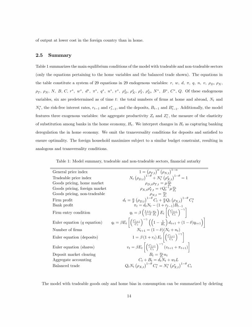
Table 1 summarizes the main equilibrium conditions of the model with tradeable and non-tradeable sectors

(only the equations pertaining to the home variables and the balanced trade shown). The equations in

the table constitute a system of 29 equations in 29 endogenous variables: r, w, d, π, q, n, v, ρD, ρX ,

ρT , ρN , N, B, C, r∗, w∗, d∗, π∗, q∗, n∗, v∗, ρ∗D, ρ

∗X , ρ

∗T , ρ

∗D, N

∗, B∗, C∗, Q. Of these endogenous

variables, six are predetermined as of time t: the total numbers of firms at home and abroad, Nt and

N∗t , the risk-free interest rates, rt−1 and r∗t−1, and the deposits, Bt−1 and B∗t−1. Additionally, the model

features three exogenous variables: the aggregate productivity Zt and Z∗t , the measure of the elasticity

of substitution among banks in the home economy, Ht. We interpret changes in Ht as capturing banking

deregulation the in home economy. We omit the transversality conditions for deposits and satisfied to

ensure optimality. The foreign household maximizes subject to a similar budget constraint, resulting in

analogous and transversality conditions.

Table 1: Model summary, tradeable and non-tradeable sectors, financial autarky

General price index 1 =¡ρT,t

¢α ¡ρN,t

¢1−αTradeable price index Nt

¡ρD,t

¢1−θ+N∗t

¡ρ∗X,t

¢1−θ= 1

Goods pricing, home market ρD,tρT,t = µwtZt

Goods pricing, foreign market ρX,tρ∗T,t = τQ−1t µwtZt

Goods pricing, non-tradeable ρN,t =wtZt

Firm profit dt =αθ

¡ρD,t

¢1−θCt +

αθQt

¡ρX,t

¢1−θC∗t

Bank profit πt = dtNt − (1 + rt−1)Bt−1Firm entry condition qt = β

³1+rt1−δ

wtZt

´Et

·³Ct+1Ct

´−γ¸Euler equation (q equation) qt = βEt

·³Ct+1Ct

´−γ ³³1− 1

Ht

´dt+1 + (1− δ)qt+1

´¸Number of firms Nt+1 = (1− δ)(Nt + nt)

Euler equation (deposits) 1 = β (1 + rt)Et

·³Ct+1Ct

´−γ¸Euler equation (shares) vt = βEt

·³Ct+1Ct

´−γ(vt+1 + πt+1)

¸Deposit market clearing Bt =

wtZtnt

Aggregate accounting Ct +Bt = dtNt + wtL

Balanced trade QtNt¡ρX,t

¢1−θC∗t = N∗t

¡ρ∗X,t

¢1−θCt

The model with tradeable goods only and home bias in consumption can be summarized by deleting

14

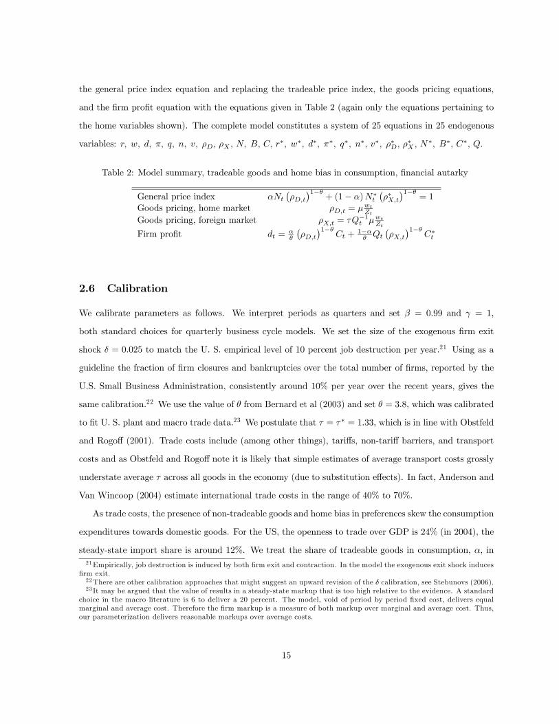
the general price index equation and replacing the tradeable price index, the goods pricing equations,

and the firm profit equation with the equations given in Table 2 (again only the equations pertaining to

the home variables shown). The complete model constitutes a system of 25 equations in 25 endogenous

variables: r, w, d, π, q, n, v, ρD, ρX , N, B, C, r∗, w∗, d∗, π∗, q∗, n∗, v∗, ρ∗D, ρ

∗X , N

∗, B∗, C∗, Q.

Table 2: Model summary, tradeable goods and home bias in consumption, financial autarky

General price index αNt¡ρD,t

¢1−θ+ (1− α)N∗t

¡ρ∗X,t

¢1−θ= 1

Goods pricing, home market ρD,t = µwtZt

Goods pricing, foreign market ρX,t = τQ−1t µwtZt

Firm profit dt =αθ

¡ρD,t

¢1−θCt +

1−αθ Qt

¡ρX,t

¢1−θC∗t

2.6 Calibration

We calibrate parameters as follows. We interpret periods as quarters and set β = 0.99 and γ = 1,

both standard choices for quarterly business cycle models. We set the size of the exogenous firm exit

shock δ = 0.025 to match the U. S. empirical level of 10 percent job destruction per year.21 Using as a

guideline the fraction of firm closures and bankruptcies over the total number of firms, reported by the

U.S. Small Business Administration, consistently around 10% per year over the recent years, gives the

same calibration.22 We use the value of θ from Bernard et al (2003) and set θ = 3.8, which was calibrated

to fit U. S. plant and macro trade data.23 We postulate that τ = τ∗ = 1.33, which is in line with Obstfeld

and Rogoff (2001). Trade costs include (among other things), tariffs, non-tariff barriers, and transport

costs and as Obstfeld and Rogoff note it is likely that simple estimates of average transport costs grossly

understate average τ across all goods in the economy (due to substitution effects). In fact, Anderson and

Van Wincoop (2004) estimate international trade costs in the range of 40% to 70%.

As trade costs, the presence of non-tradeable goods and home bias in preferences skew the consumption

expenditures towards domestic goods. For the US, the openness to trade over GDP is 24% (in 2004), the

steady-state import share is around 12%. We treat the share of tradeable goods in consumption, α, in21Empirically, job destruction is induced by both firm exit and contraction. In the model the exogenous exit shock induces

firm exit.22There are other calibration approaches that might suggest an upward revision of the δ calibration, see Stebunovs (2006).23 It may be argued that the value of results in a steady-state markup that is too high relative to the evidence. A standard

choice in the macro literature is 6 to deliver a 20 percent. The model, void of period by period fixed cost, delivers equalmarginal and average cost. Therefore the firm markup is a measure of both markup over marginal and average cost. Thus,our parameterization delivers reasonable markups over average costs.

15

the economy with tradeable and non-tradeable goods, and the weight of home goods in the consumption

basket, α, in the economy with tradable goods only and home bias in consumption as free parameters

to match the observed steady-state import share in the US given the trade cost τ = τ∗ = 1.33.24 The

values of α’s vary among the models to be considered, but in general the share of tradeable goods in

consumption, α, is around 0.39 and the weight of home goods in the consumption basket, α, is around

0.75.

We set steady-state aggregate productivity, Z, and aggregate labor endowment, L, equal to one

without loss of generality. These parameters determine the size of economy, but leave the model dynamics

unaffected. We set steady-state H (H∗), the measure of the elasticity of substitution among banks in the

home (foreign) economy), such that it implies a bank markup of about 10 percentage points. Then to

determine the size of a permanent deregulation shock, we calculate the change in H that induces a 30%

increase in the number of firms in home country (the US). Note that according to Davis et al (2006) the

number of firms (both total and privately held) increased by around 34% between 1980 and 2000, hence

we attribute most of the increase to deregulation effects. We pursue the same calibration strategy of H

for computation of the second moments in the international business cycle.

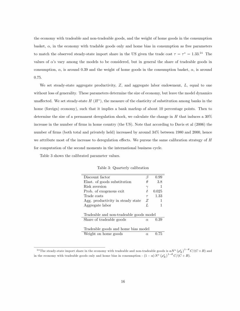
Table 3 shows the calibrated parameter values.

Table 3: Quarterly calibration

Discount factor β 0.99Elast. of goods substitution θ 3.8Risk aversion γ 1Prob. of exogenous exit δ 0.025Trade costs τ 1.33Agg. productivity in steady state Z 1Aggregate labor L 1

Tradeable and non-tradeable goods modelShare of tradeable goods α 0.39

Tradeable goods and home bias modelWeight on home goods α 0.75

24The steady-state import share in the economy with tradeable and non-tradeable goods is αN∗¡ρ∗X¢1−θ

C/(C+B) and

in the economy with tradeable goods only and home bias in consumption - (1− α)N∗¡ρ∗X¢1−θ

C/(C +B).

16

2.7 Deregulation and macroeconomic dynamics

We now analyze the response path of the real exchange rate and other key variables in response to

permanent deregulation in the home economy. (We assume that the foreign economy does not deregulate.)

To do so, we log-linearize the system of equilibrium conditions in Table 1 (and in Table 2) around the

symmetric steady state. (All endogenous variables are constant in steady state. All exogenous variables,

including aggregate productivity, are constant in steady state.)

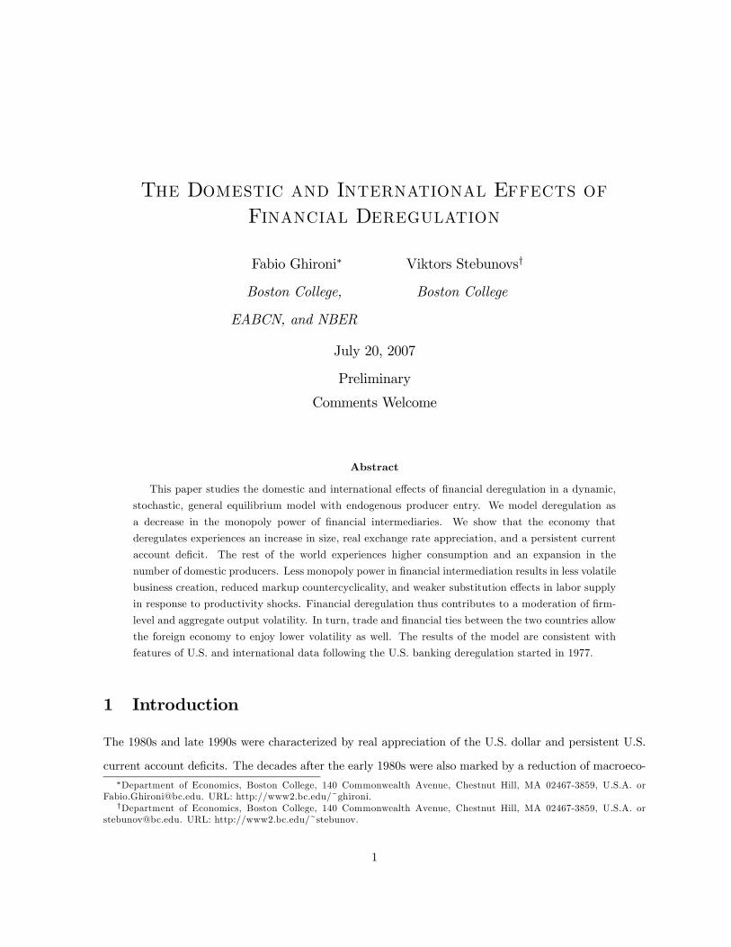
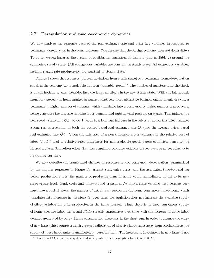
Figures 1 shows the responses (percent deviations from steady state) to a permanent home deregulation

shock in the economy with tradeable and non-tradeable goods.25 The number of quarters after the shock

is on the horizontal axis. Consider first the long-run effects in the new steady state. With the fall in bank

monopoly power, the home market becomes a relatively more attractive business environment, drawing a

permanently higher number of entrants, which translates into a permanently higher number of producers,

hence generates the increase in home labor demand and puts upward pressure on wages. This induces the

new steady state for TOLt below 1, leads to a long-run increase in the prices at home, this effect induces

a long-run appreciation of both the welfare-based real exchange rate Qt (and the average prices-based

real exchange rate eQt). Given the existence of a non-tradeable sector, changes in the relative cost oflabor (TOLt) lead to relative price differences for non-tradeable goods across countries, hence to the

Harrod-Balassa-Samuelson effect (i.e. less regulated economy exhibits higher average prices relative to

its trading partner).

We now describe the transitional changes in response to the permanent deregulation (summarized

by the impulse responses in Figure 1). Absent sunk entry costs, and the associated time-to-build lag

before production starts, the number of producing firms in home would immediately adjust to its new

steady-state level. Sunk costs and time-to-build transform Nt into a state variable that behaves very

much like a capital stock: the number of entrants nt represents the home consumers’ investment, which

translates into increases in the stock Nt over time. Deregulation does not increase the available supply

of effective labor units for production in the home market. Thus, there is no short-run excess supply

of home effective labor units, and TOLt steadily appreciates over time with the increase in home labor

demand generated by entry. Home consumption decreases in the short run, in order to finance the entry

of new firms (this requires a much greater reallocation of effective labor units away from production as the

supply of these labor units is unaffected by deregulation). The increase in investment in new firms is not25Given τ = 1.33, we se the weight of tradeable goods in the consumption basket, α, to 0.397.

17

0 4 8 12 16 20 24 28 32 36 40 44-0.1

-0.05

0

0.05

0.1Consumption, home (C)

0 4 8 12 16 20 24 28 32 36 40 44-4

-2

0

2

4

6x 10

-3 Consumption, foreign (C*)

0 4 8 12 16 20 24 28 32 36 40 440

0.2

0.4

0.6

0.8Firms, home (N)

0 4 8 12 16 20 24 28 32 36 40 44-5

-4

-3

-2

-1

0x 10

-9 Firms, foreign (N*)

0 4 8 12 16 20 24 28 32 36 40 44-0.2

-0.15

-0.1

-0.05

0Terms of labor (TOL)

0 4 8 12 16 20 24 28 32 36 40 44-0.1

-0.08

-0.06

-0.04

-0.02

0Real exchange rate (Q)

0 4 8 12 16 20 24 28 32 36 40 44-0.01

0

0.01

0.02

0.03

0.04Adj. aggregate output,home (Y~)

0 4 8 12 16 20 24 28 32 36 40 44-0.04

-0.03

-0.02

-0.01

0Adj. aggregate output, foreign (Y~*)

Figure 1: Response to permanent deregulation shock in the economy with tradeable and non-tradeablegoods (financial autarky).

sufficient to offset the decrease in consumption in the early stages of the transition, hence the aggregate

output falls initially. We note that the real exchange rate appreciation is slow to unfold. About half of

the long-run appreciation occurs after the first year and a half of the permanent deregulation shock, and

reaching the long-run level takes over 7 years.

The notable externality of deregulation in home is the significant decline of the aggregate output in

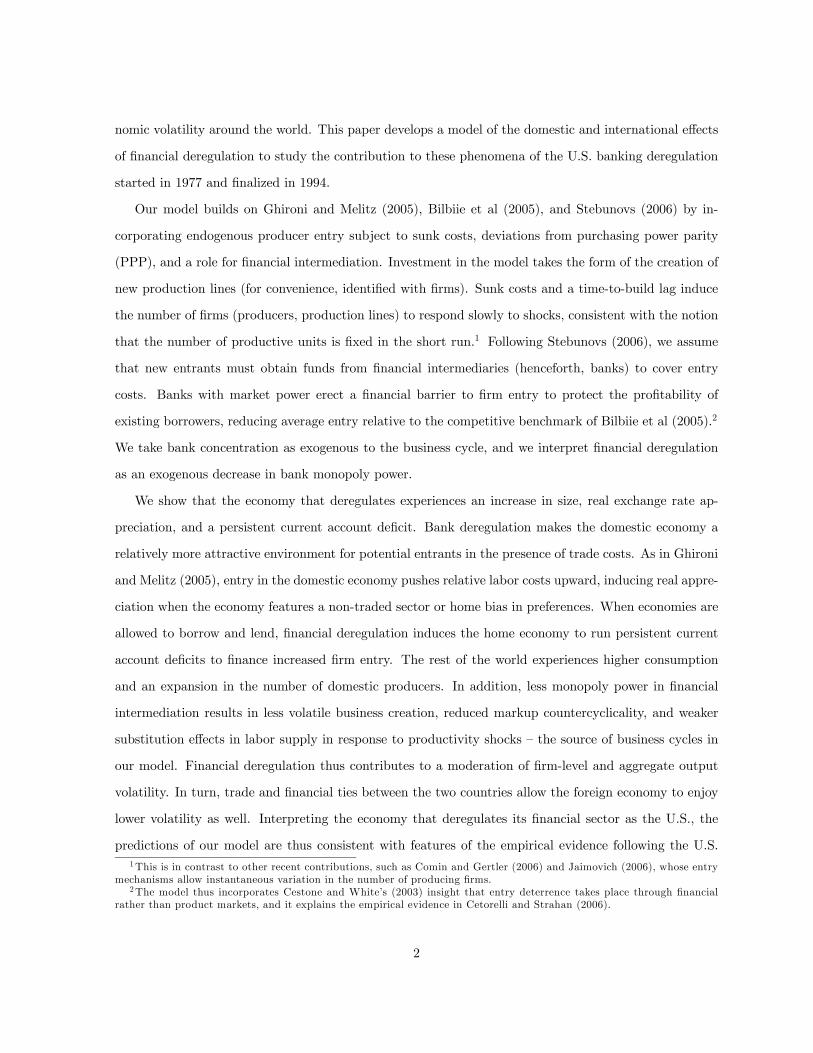
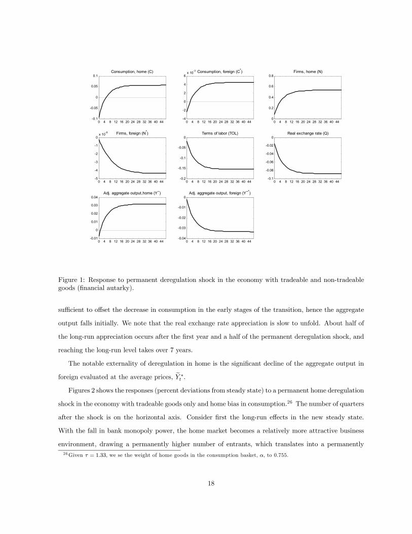
foreign evaluated at the average prices, eY ∗t .Figures 2 shows the responses (percent deviations from steady state) to a permanent home deregulation

shock in the economy with tradeable goods only and home bias in consumption.26 The number of quarters

after the shock is on the horizontal axis. Consider first the long-run effects in the new steady state.

With the fall in bank monopoly power, the home market becomes a relatively more attractive business

environment, drawing a permanently higher number of entrants, which translates into a permanently26Given τ = 1.33, we se the weight of home goods in the consumption basket, α, to 0.755.

18

higher number of producers. This induces the new steady state for TOLt below 1. This appreciation of

home labor costs leads to a long-run increase in the average prices at home (due the presence of home bias

in consumption), this effect induces a long-run appreciation of the real exchange rate eQt. Our simulationssuggest that the increase in product variety for home consumers dominates the average price appreciation,

leading to a depreciation of the welfare-based index Qt. Consumers in both countries would rather spend

a given nominal expenditure in the home market, even though average prices there are relatively higher.

0 4 8 12 16 20 24 28 32 36 40 44-0.2

-0.1

0

0.1

0.2Consumption, home (C)

0 4 8 12 16 20 24 28 32 36 40 44-4

-2

0

2

4x 10

-3 Consumption, foreign (C*)

0 4 8 12 16 20 24 28 32 36 40 440

0.2

0.4

0.6

0.8Firms, home (N)

0 4 8 12 16 20 24 28 32 36 40 44-1

0

1

2

3

4x 10

-10 Firms, foreign (N*)

0 4 8 12 16 20 24 28 32 36 40 44-0.2

-0.15

-0.1

-0.05

0Terms of labor (TOL)

0 4 8 12 16 20 24 28 32 36 40 44-0.03

-0.02

-0.01

0

0.01

0.02Real exchange rate (Q)

0 4 8 12 16 20 24 28 32 36 40 44-0.08

-0.06

-0.04

-0.02

0Adjusted real exchange rate (Q~)

0 4 8 12 16 20 24 28 32 36 40 44-0.04

-0.02

0

0.02

0.04Adj. aggregate output,home (Y~)

0 4 8 12 16 20 24 28 32 36 40 44-0.05

-0.04

-0.03

-0.02

-0.01

0Adj. aggregate output, foreign (Y~*)

Figure 2: Response to permanent deregulation shock in the economy with tradeable goods only and homebias in consumption (financial autarky).

We now describe the transitional changes in response to the permanent deregulation (summarized by

the impulse responses in Figure 2). The number of producing firms in home gradually adjusts to its new

steady-state level. There is no short-run excess supply of home effective labor units, and TOLt steadily

appreciates over time with the increase in home labor demand generated by entry. Home consumption

decreases in the short run, in order to finance the entry of new firms (this requires a much greater

reallocation of effective labor units away from production as the supply of these labor units is unaffected

19

by deregulation). The increase in investment in new firms is not sufficient to offset the decrease in

consumption in the early stages of the transition, hence the aggregate output falls initially. We note that

the real exchange rate appreciation is slow to unfold. About half of the long-run appreciation occurs after

the first two years of the permanent deregulation shock, and reaching the long-run level takes about 10

years.

The notable externality of deregulation in home is the significant decline of the aggregate output in

foreign evaluated at the average prices, eY ∗t .3 International deposits

We now extend the model of previous section to allow for international trade in deposits. We study

how international deposit trading affects the results we have previously described and how our new

microeconomic dynamics affect the current account. Since the extension to international deposits does

not involve especially innovative features relative to the financial autarky setup, we herein limit ourselves

to describing its main ingredients in words and present the relevant model equations in Table 6 in the

Appendix.

We assume that banks can supply deposits domestically and internationally. Home deposits, issued

to home and foreign households, are denominated in home currency. Foreign deposits, issued to home

and foreign households, are denominated in foreign currency. We maintain the assumption that nominal

returns are indexed to inflation in each country, so that deposits issued by each country provide a risk-free,

real return in units of that country’s consumption basket. International asset markets are incomplete,

as only risk-free deposits are traded across countries. In the absence of any other change to our model,

this would imply indeterminacy of steady-state net foreign assets and nonstationarity. To resolve these

issues, we assume that agents must pay fees to domestic banks when adjusting their deposits. We assume

that these fees are a quadratic function of the stock of deposits. This convenient specification is sufficient

to uniquely pin down the steady state and deliver stationary model dynamics in response to temporary

shocks. Realistic choices of parameter values imply that the cost of adjusting deposit holdings has a very

small impact on model dynamics, other than pinning down the steady state and ensuring mean reversion

in the long run when shocks are transitory. We set the scale parameter for the deposit adjustment cost, η,

to 0.0025 - sufficient to generate stationarity in response to transitory shocks but small enough to avoid

20

overstating the role of this friction in determining the international business cycle dynamics of our model.

However, in simulations of a permanent deregulation shock, which we do not interpreted as a business

cycle frequency shock, we set the scale parameter for the deposit adjustment cost, η, close to zero.

We assume that banks rebate the revenues from deposit adjustment fees to domestic households.

In equilibrium, the markets for home and foreign deposits clear, and each country’s net foreign assets

entering period t + 1 depend on interest income from asset holdings entering period t, labor income,

net investment income, and consumption during period t. The change in asset holdings between t and

t + 1 is the country’s current account. Home and foreign current accounts add to zero when expressed

in units of the same consumption basket. There are now three Euler equations in each country: the

Euler equation for share holdings, which is unchanged, and Euler equations for holdings of domestic

and foreign deposits. The fees for adjusting deposits imply that the Euler equations for deposits feature

a term that depends on the stock of deposits - a key ingredient delivering determinacy of the steady

state and model stationarity. Euler equations for deposits in each country imply a no-arbitrage condition

between deposits. In the log-linear model, this no-arbitrage condition relates (in a standard fashion)

the real interest rate differential across countries to expected depreciation of the consumption-based real

exchange rate. The balanced trade condition closed the model under financial autarky. Since trade is

no longer balanced under international deposit trading, we must explicitly impose labor market clearing

conditions in both countries. These conditions state that the amount of labor used in production and to

cover entry costs in each country must equal labor supply in that country in each period.

The costs of adjusting deposits do not imply zero holdings of foreign deposits by home and vice versa

in the symmetric steady state. Thus, the extended model with international deposit trading does not

feature the same steady state as the model under financial autarky. We now consider the home economy.

The deposit interest rate depends on the investment into new firms, 1 + r = 1β

¡1 + η 12

wZn¢, and home

and foreign deposits each cover half of the investment, B = B∗ = 12wZn. Similar equations hold abroad.

As before, we analyze the response path of the real exchange rate and other key variables in response

to the same permanent deregulation. To do so, we log-linearize the system of equilibrium conditions in

Table 6 around the symmetric steady state.

21

3.1 Deregulation and macroeconomic dynamics

We consider the deregulation shocks as under financial autarky (however, the shock size have to be

recalibrated). The response of several key variables to the shock is qualitatively similar to that under

financial autarky.

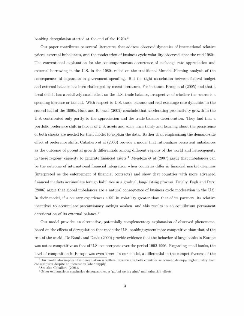
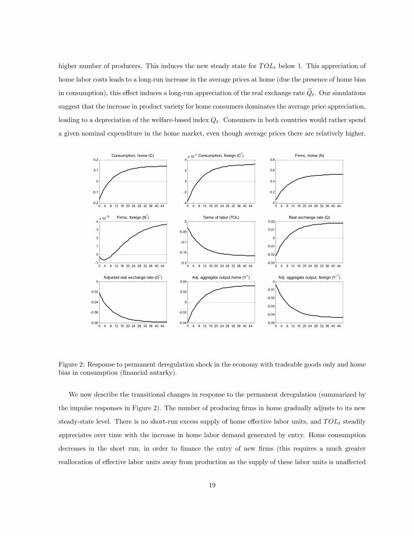
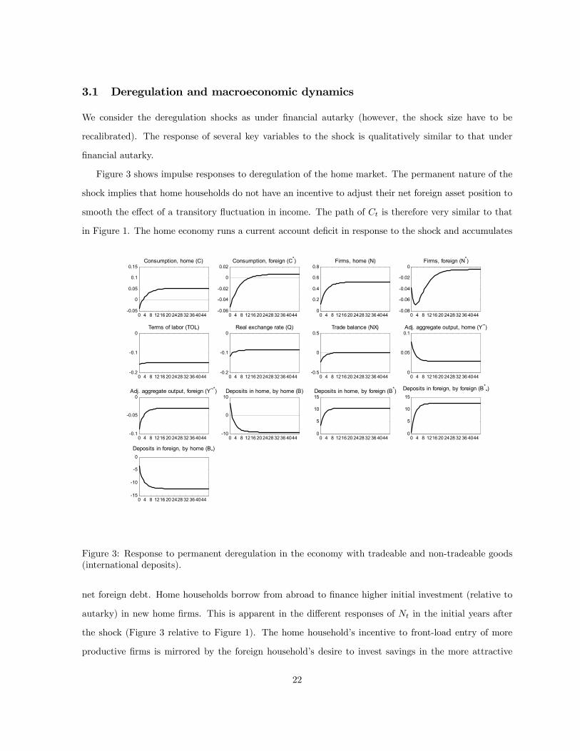
Figure 3 shows impulse responses to deregulation of the home market. The permanent nature of the

shock implies that home households do not have an incentive to adjust their net foreign asset position to

smooth the effect of a transitory fluctuation in income. The path of Ct is therefore very similar to that

in Figure 1. The home economy runs a current account deficit in response to the shock and accumulates

0 4 8 1216 20 2428 32 36 4044-0.05

0

0.05

0.1

0.15Consumption, home (C)

0 4 8 1216 20 2428 32 36 4044-0.06

-0.04

-0.02

0

0.02Consumption, foreign (C*)

0 4 8 1216 20 2428 32 36 40440

0.2

0.4

0.6

0.8Firms, home (N)

0 4 8 1216 20 2428 32 36 4044-0.08

-0.06

-0.04

-0.02

0Firms, foreign (N*)

0 4 8 1216 20 2428 32 36 4044-0.2

-0.1

0Terms of labor (TOL)

0 4 8 1216 20 2428 32 36 4044-0.2

-0.1

0Real exchange rate (Q)

0 4 8 1216 20 2428 32 36 4044-0.5

0

0.5Trade balance (NX)

0 4 8 1216 20 2428 32 36 40440

0.05

0.1Adj. aggregate output, home (Y~)

0 4 8 1216 20 2428 32 36 4044-0.1

-0.05

0Adj. aggregate output, foreign (Y~*)

0 4 8 1216 20 2428 32 36 4044-10

0

10Deposits in home, by home (B)

0 4 8 1216 20 2428 32 36 40440

5

10

15Deposits in home, by foreign (B*)

0 4 8 1216 20 2428 32 36 40440

5

10

15

Deposits in foreign, by foreign (B**)

0 4 8 1216 20 2428 32 36 4044-15

-10

-5

0

Deposits in foreign, by home (B*)

Figure 3: Response to permanent deregulation in the economy with tradeable and non-tradeable goods(international deposits).

net foreign debt. Home households borrow from abroad to finance higher initial investment (relative to

autarky) in new home firms. This is apparent in the different responses of Nt in the initial years after

the shock (Figure 3 relative to Figure 1). The home household’s incentive to front-load entry of more

productive firms is mirrored by the foreign household’s desire to invest savings in the more attractive

22

economy. Home consumption initially declines and is permanently higher in the long run. Foreign

consumption moves by more than in Figure 1 as foreign households initially save in the form of foreign

lending and then receive income from their positive asset position. Although foreign households cannot

hold shares in the mutual fund of home banks (since only international deposits can be traded across

countries), the return on deposit holdings is tied to the return on holdings of shares in home banks by

no-arbitrage between bonds and shares within the home economy. Therefore, foreign households share

the benefits of expansion in the home economy via international deposit holdings. As in the case of

financial autarky, TOLt must decrease in the long run (home effective labor must relatively appreciate);

otherwise, all new entrants would choose to locate in the home economy. The accelerated entry of

new home firms induces an immediate relative increase in home labor demand and TOLt immediately

appreciates (as opposed to a gradual appreciation under financial autarky). Thus, the real exchange rate

Qt (and eQt) also immediately appreciates. The opening of the economy to international deposit tradingdoes not qualitatively change the functioning of the HBS mechanism in our model. The notable long-run

externalities of deregulation in home are a significant decline of the aggregate output in foreign evaluated

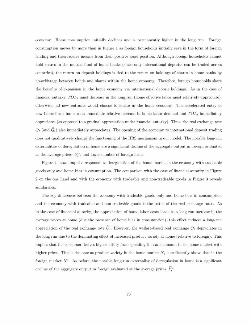
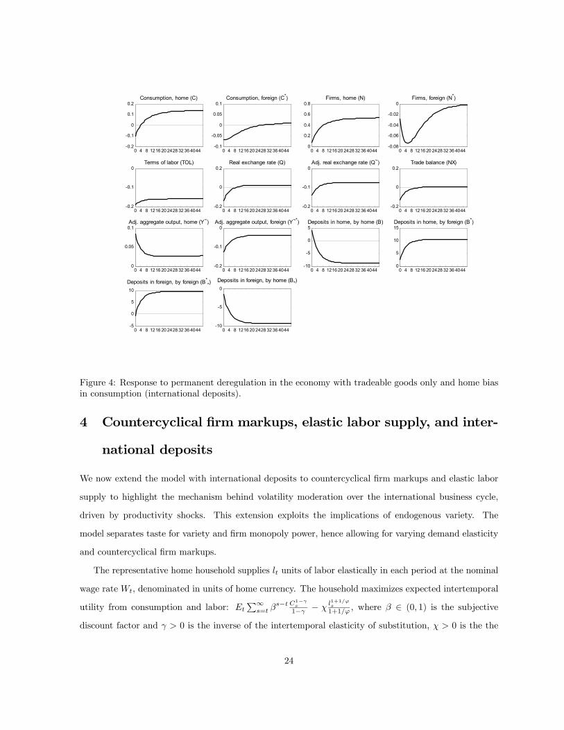
at the average prices, eY ∗t , and lower number of foreign firms.Figure 4 shows impulse responses to deregulation of the home market in the economy with tradeable

goods only and home bias in consumption. The comparison with the case of financial autarky in Figure

2 on the one hand and with the economy with tradeable and non-tradeable goods in Figure 3 reveals

similarities.

The key difference between the economy with tradeable goods only and home bias in consumption

and the economy with tradeable and non-tradeable goods is the paths of the real exchange rates. As

in the case of financial autarky, the appreciation of home labor costs leads to a long-run increase in the

average prices at home (due the presence of home bias in consumption), this effect induces a long-run

appreciation of the real exchange rate eQt. However, the welfare-based real exchange Qt depreciates inthe long run due to the dominating effect of increased product variety at home (relative to foreign). This

implies that the consumer derives higher utility from spending the same amount in the home market with

higher prices. This is the case as product variety in the home market Nt is sufficiently above that in the

foreign market N∗t . As before, the notable long-run externality of deregulation in home is a significant

decline of the aggregate output in foreign evaluated at the average prices, eY ∗t .

23

0 4 8 1216 20 2428 32 36 4044-0.2

-0.1

0

0.1

0.2Consumption, home (C)

0 4 8 1216 20 2428 32 36 4044-0.1

-0.05

0

0.05

0.1Consumption, foreign (C*)

0 4 8 1216 20 2428 32 36 40440

0.2

0.4

0.6

0.8Firms, home (N)

0 4 8 1216 20 2428 32 36 4044-0.08

-0.06

-0.04

-0.02

0Firms, foreign (N*)

0 4 8 1216 20 2428 32 36 4044-0.2

-0.1

0Terms of labor (TOL)

0 4 8 1216 20 2428 32 36 4044-0.2

0

0.2Real exchange rate (Q)

0 4 8 1216 20 2428 32 36 4044-0.2

-0.1

0Adj. real exchange rate (Q~)

0 4 8 1216 20 2428 32 36 4044-0.2

0

0.2Trade balance (NX)

0 4 8 1216 20 2428 32 36 40440

0.05

0.1Adj. aggregate output, home (Y~)

0 4 8 1216 20 2428 32 36 4044-0.2

-0.1

0Adj. aggregate output, foreign (Y~*)

0 4 8 1216 20 2428 32 36 4044-10

-5

0

5Deposits in home, by home (B)

0 4 8 1216 20 2428 32 36 40440

5

10

15Deposits in home, by foreign (B*)

0 4 8 1216 20 2428 32 36 4044-5

0

5

10

Deposits in foreign, by foreign (B**)

0 4 8 1216 20 2428 32 36 4044-10

-5

0

Deposits in foreign, by home (B*)

Figure 4: Response to permanent deregulation in the economy with tradeable goods only and home biasin consumption (international deposits).

4 Countercyclical firm markups, elastic labor supply, and inter-

national deposits

We now extend the model with international deposits to countercyclical firm markups and elastic labor

supply to highlight the mechanism behind volatility moderation over the international business cycle,

driven by productivity shocks. This extension exploits the implications of endogenous variety. The

model separates taste for variety and firm monopoly power, hence allowing for varying demand elasticity

and countercyclical firm markups.

The representative home household supplies lt units of labor elastically in each period at the nominal

wage rate Wt, denominated in units of home currency. The household maximizes expected intertemporal

utility from consumption and labor: EtP∞

s=t βs−t C1−γ

s

1−γ − χl1+1/ϕs

1+1/ϕ , where β ∈ (0, 1) is the subjectivediscount factor and γ > 0 is the inverse of the intertemporal elasticity of substitution, χ > 0 is the the

24

weight of disutility of labor effort and ϕ > 0 is the Frisch elasticity of labor supply to wages, subject to the

same budget constraint as in the previous section. The household’s intertemporal optimality conditions

remain the same, the only additional intratemporal condition is the optimality condition for labor supply.

Elastic labor supply implies that households have an extra margin of adjustment to aggregate productivity

shocks, as in Bilbiie et al (2006). This enhances the propagation mechanism of the model by amplifying

the responses of endogenous variables with respect to the benchmark model. As before we consider two

definitions of the basket of goods Ct. However, now we define the basket goods over discrete varieties.

Given that the number of firms is endogenous, one cannot assume that the number is sufficiently large

for the weight of each producer to be negligible.

First, we consider the economy with tradeable and non-tradeable goods. The basket of tradeable

goods now is CT,t =³X

ω∈Ω ct(ω)(θ−1)/θdω

´θ/(θ−1), hence PT,t =

³Pω∈Ωt (pt(ω))

1−θdω´1/(1−θ)

. Each

producer no longer ignores the effects of its nominal domestic price, pD,t(ω), on the home tradeable

price index, PT,t, and the effect of its nominal export price, pX,t(ω), on the foreign tradeable price

index, P ∗T,t.27 The perceived home demand elasticities is then εD,t(ω) = θ

³1− (pD,t(ω)/PT,t)1−θ

´and

the foreign demand elasticity is εX,t(ω) = θ³1− ¡pX,t(ω)/P ∗T,t¢1−θ´. Note that taking into account

this indirect price effect decreases the elasticities perceived by firm ω, εD,t(ω) < θ and εX,t(ω) < θ,

hence increases its monopoly power in both markets. The implied firm markup in domestic market is

µD,t(ω) = εD,t(ω)/ (εD,t(ω)− 1) and in foreign market µX,t(ω) = εX,t(ω)/ (εX,t(ω)− 1).28 Firms set

flexible prices that reflect the different markups over marginal cost. Prices, in real terms relative to

the price index in the destination market, are then given by ρD,t(ω)ρT,t(ω) = pD,t(ω)/PT,tPT,t/Pt =

µD,t(ω)wt/Zt and ρX,t(ω)ρ∗T,t(ω) = pX,t(ω)/P

∗T,tP

∗T,t/P

∗t = Q−1t τµX,t(ω)wt/Zt. A firm decomposes its

total profit into two portions earned from domestic sales dD,t(ω) (d∗D,t(ω)) and from export sales dX,t(ω)

(d∗X,t(ω)). In the case of a home firm, the portions of total profits are dD,t(ω) = α/εD,t¡ρD,t

¢1−θCt and

dX,t = α/εX,tQt¡ρX,t

¢1−θC∗t .29 Since all firms are identical in equilibrium, one may drop indexing by

ω. In this economy the bank internalizes the effect of entry on firm profits through the effect of entry on

the nominal domestic price, pD,t, and then on the home tradeable goods price index, PT,t, and the effect27See Yang and Heijdra (1993) for the treatment of Dixit-Stiglitz model of monopolistic competition with discrete number

of producers.28As it turns out firm entry is procyclical, hence firm markups are countercyclical and work to amplify, rather than

stabilize, movements in firm output.29 Similar price equations hold for foreign firms, though note that ρ∗X,t(ω)ρT,t(ω) = p∗X,t(ω)/PT,tPT,t/Pt =

Qtτ∗µ∗X,t(ω)w∗t /Z

∗t , and hence a foreign firm earns export profits d∗X,t = α/ε∗X,tQ

−1t

³ρ∗X,t

´1−θCt.

25

of entry on the nominal export price, pX,t, and then on the foreign tradeable goods price index, P ∗T,t.

Second, we consider the economy with tradeable goods only and home bias in consumption. The

baskets of home and foreign goods now are defined as cD,t =³X

ω∈Ω cD,t(ω)(θ−1)/θdω

´θ/(θ−1)and

cX,t =³X

ω∗∈Ω cX,t(ω∗)(θ−1)/θdω∗

´θ/(θ−1)and the corresponding price indices for home and foreign

baskets are pD,t =¡P

ω∈Ωt pD,t(ω)1−θdω

¢1/(1−θ)and p∗X,t =

¡Pω∗∈Ωt p

∗X,t(ω

∗)1−θdω∗¢1/(1−θ)

. As above

each producer no longer ignores the effects of its nominal domestic price, pD,t(ω), on the home general

price index, Pt, and the effect of its nominal export price, pX,t(ω), on the foreign general price index,

P ∗t . The perceived home demand elasticities is then εD,t(ω) = θ³1− (pD,t(ω)/Pt)1−θ

´and the foreign

demand elasticity is εX,t(ω) = θ³1− (pX,t(ω)/P ∗t )1−θ

´. The implied firm markup in domestic market is

µD,t(ω) = εD,t(ω)/ (εD,t(ω)− 1) and in foreign market µX,t(ω) = εX,t(ω)/ (εX,t(ω)− 1). Prices, in realterms relative to the price index in the destination market, are then given by ρD,t(ω) = pD,t(ω)/Pt =

µD,t(ω)wt/Zt and ρX,t(ω) = pX,t(ω)/P∗t = Q

−1t τµX,t(ω)wt/Zt. Similar price equations hold for foreign

firms. A firm decomposes its total profit into two portions earned from domestic sales dD,t(ω) (d∗D,t(ω))

and from export sales dX,t(ω) (d∗X,t(ω)). In the case of a home firm, the portions of total profits are

dD,t(ω) = α/εD,t¡ρD,t

¢1−θCt and dX,t = (1− α) /εX,tQt

¡ρX,t

¢1−θC∗t . Foreign firms behave in a similar

way. Since all firms are identical in equilibrium, one may drop indexing by ω. In this economy, the bank

internalizes the effect of entry on firm profits through the effect of entry on the nominal domestic price,

pD,t, and then on the home general price index, Pt, and the effect of entry on the nominal export price,

pX,t, and then on the foreign general price index, P ∗t .

In both the economy with tradeable and non-tradeable goods and the economy with tradeable goods

only and home bias in consumption, the new equation for firm value, qt, becomes:

qt = βEt

"µCt+1Ct

¶−γ µµ1− 1

H

θ

εD,t+1

¶dD,t+1 +

µ1− 1

H

θ

εX,t+1

¶dX,t+1 + (1− δ)qt+1

¶#. (3)

(The derivation details are given in Appendix. A similar equation holds aboard.) The parameter H plays

in bank market the same role that θ plays in goods market. At one extreme, H = 1 or absolute bank

monopoly, equation (2) says that there is no entry as the marginal (and average) return from funding an

entrant is negative: the portfolio expansion effect is dominated by profit destruction effect. The model

displays a gradual reduction in market power as the measure of the elasticity of substitution across banks,

H, increases. At the other extreme, H =∞, the equation simplifies to the usual asset pricing equation.

26

Over the business cycle, as the number of firms increases, the perceived demand elasticities εD,t and εX,t

increase, hence markups fall. On the one hand, the fall in firm markups reduces the bank’s incentive to

invest in new firms. (Note that the ratios θ/εD,t+1 and θ/εX,t+1are larger than one.) But on the other

hand, since the aggregate firm profit is procyclical and the bank has claims on it, the importance of profit

destruction externality, θ/εD,t+1 and θ/εX,t+1, falls, thus increasing the bank’s incentive to invest.

Table 1 summarizes the main equilibrium conditions of the model with tradeable and non-tradeable

sectors (only the equations pertaining to the home variables and the balanced trade shown). The model

with tradeable goods only and home bias in consumption can be summarized by deleting the general

price index equation and replacing the tradeable price index, the goods pricing equations, the firm profit

equation, and the labor clearing equation with the equations given in Table 2 (again only the equations

pertaining to the home variables shown).

We examine the model predictions under Frisch elasticity, ϕ, of ten.30 We set the weight of disutility

of labor, χ, to one. The household preference, exogenous exit parameters remain the same as in the

benchmark model (see Table 3).31 The calibration strategy of a’s and H are the same as before. We pick

a’s that match the 12% imports over GDP ratio observed for the US given τ = τ∗ = 1.33. We then pick

the value of H before deregulation that implies a bank markup of 10 percentage points. Then a 30%

increase in the number of domestic firms pins down the value of H after deregulation. We use the two

values of H to determine the size of a permanent deregulation shock, and then for computation of the

second moments in the international business cycle. We keep the steady-state aggregate productivity,

Z, set to one. Note though that it is no longer just a scale parameter. It not only determines the

number of firms (the size of the economy ) in steady state and hence the steady-state firm markups, but

also the cyclical properties of markups. The lower the steady-state aggregate productivity is, the lower

is the number of firms and the higher are firm markups in steady state and the more countercyclical

markups are over the business cycle. In fact, by adjusting the steady-state aggregate productivity we can

affect the interplay of wealth and substitution effects in labor supply decisions. As lower steady-state

aggregate productivity leads to more countercyclical markups, and hence more procyclical wages, it helps

to generate stronger substitution effects and weaker wealth effect (on temporary domestic productivity

shock impact) in labor supply decisions. The representative household then is willing to take advantage of30The case in which ϕ→∞ corresponds to linear disutility of effort and is often studied in the business cycle literature.31King et al (1988) show that under separable preferences, log utility of consumption ensures that income and substitution

effects or real wage variation on effort cancel out in steady state. This guarantees constant steady state effort and is necessaryfor balanced growth under trend productivity growth.

27

the temporary high productivity by supplying more labor to increase substantially the available number of

varieties, lower firm monopoly power, and experience much higher consumption in the future. Two things

are crucial for the strength of this mechanism. First, the elasticity of intertemporal substitution (and

little or no habit formation in consumption) should be relative high, so that the representative household

is not overly engaged in consumption smoothing. Second, as usual, the persistence of a productivity

shock increases the strength of wealth effect, as when the representative household does not expect to

change consumption much in the future, the household thus simply takes this opportunity to increase

consumption of leisure.

4.1 Deregulation and macroeconomic dynamics

We consider the deregulation shocks as international deposits, inelastic labor supply, and constant firm

markups (however, the shock size have to be recalibrated). The response of several key variables to the

shock is qualitatively similar to that under financial autarky.

In this and the following sections, the share of tradeable goods in consumption basket, α, in the

economy with tradeable and non-tradeable goods is set to 0.5, while the iceberg cost, τ , is kept at 1.33.32

This choice of α is dictated by computational difficulties in finding the model’s steady state, and it implies

the steady-state import share of about 18%. In the economy with tradeable goods only and home bias

in consumption, given τ = 1.33, we set the weight of home goods in the consumption basket, α, to 0.797,

which gives the steady-state import share of about 12%.

Figure 5 shows impulse responses to deregulation of the home market in the economy with tradeable

and non-tradeable goods. The response of several key variables to the shock is qualitatively similar to

that under international deposits, inelastic labor supply, and constant firm markups, but there are several

new features as well. The home economy runs a current account deficit in response to the shock and

accumulates net foreign debt. Home households borrow from abroad to finance higher initial investment

(relative to the international deposit model in the previous section) in new home firms. This is apparent

in the different responses of Nt in the initial years after the shock. The home household’s incentive to

front-load entry of more productive firms is mirrored by the foreign household’s desire to invest savings

in the more attractive economy. Notably, home consumption does not initially decline and, as before,

is permanently higher in the long run. Foreign consumption moves by more than in Figure 3 as foreign32The lowest steady-state import share given τ = 1.33 we were able to obtain was 16% under α approaching 0.35.

28

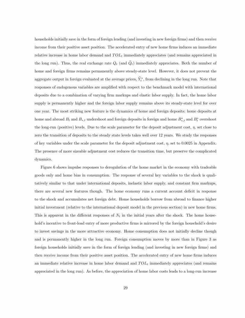
households initially save in the form of foreign lending (and investing in new foreign firms) and then receive

income from their positive asset position. The accelerated entry of new home firms induces an immediate

relative increase in home labor demand and TOLt immediately appreciates (and remains appreciated in

the long run). Thus, the real exchange rate Qt (and eQt) immediately appreciates. Both the number ofhome and foreign firms remains permanently above steady-state level. However, it does not prevent the

aggregate output in foreign evaluated at the average prices, eY ∗t , from declining in the long run. Note thatresponses of endogenous variables are amplified with respect to the benchmark model with international

deposits due to a combination of varying firm markups and elastic labor supply. In fact, the home labor

supply is permanently higher and the foreign labor supply remains above its steady-state level for over

one year. The most striking new feature is the dynamics of home and foreign deposits: home deposits at

home and abroad Bt and B∗,t undershoot and foreign deposits in foreign and home B∗∗,t and B∗t overshoot

the long-run (positive) levels. Due to the scale parameter for the deposit adjustment cost, η, set close to

zero the transition of deposits to the steady state levels takes well over 12 years. We study the responses

of key variables under the scale parameter for the deposit adjustment cost, η, set to 0.0025 in Appendix.

The presence of more sizeable adjustment cost reduces the transition time, but preserve the complicated

dynamics.

Figure 6 shows impulse responses to deregulation of the home market in the economy with tradeable

goods only and home bias in consumption. The response of several key variables to the shock is quali-

tatively similar to that under international deposits, inelastic labor supply, and constant firm markups,

there are several new features though. The home economy runs a current account deficit in response

to the shock and accumulates net foreign debt. Home households borrow from abroad to finance higher

initial investment (relative to the international deposit model in the previous section) in new home firms.

This is apparent in the different responses of Nt in the initial years after the shock. The home house-

hold’s incentive to front-load entry of more productive firms is mirrored by the foreign household’s desire

to invest savings in the more attractive economy. Home consumption does not initially decline though

and is permanently higher in the long run. Foreign consumption moves by more than in Figure 3 as

foreign households initially save in the form of foreign lending (and investing in new foreign firms) and

then receive income from their positive asset position. The accelerated entry of new home firms induces

an immediate relative increase in home labor demand and TOLt immediately appreciates (and remains

appreciated in the long run). As before, the appreciation of home labor costs leads to a long-run increase

29

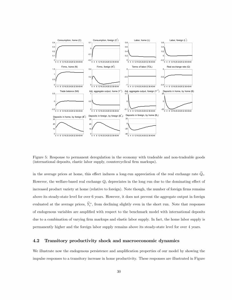
0 4 8 1216 20 2428 32 36 40440

0.1

0.2

0.3

0.4Consumption, home (C)

0 4 8 1216 20 2428 32 36 4044-0.2

-0.1

0

0.1Consumption, foreign (C*)

0 4 8 1216 20 2428 32 36 40440

0.2

0.4

0.6

0.8Labor, home (L)

0 4 8 1216 20 2428 32 36 4044-0.2

0

0.2

0.4

0.6Labor, foreign (L*)

0 4 8 1216 20 2428 32 36 40440

0.5

1

1.5Firms, home (N)

0 4 8 1216 20 2428 32 36 40440

0.2

0.4Firms, foreign (N*)

0 4 8 1216 20 2428 32 36 4044-1

-0.5

0Terms of labor (TOL)

0 4 8 1216 20 2428 32 36 4044-0.4

-0.2

0Real exchange rate (Q)

0 4 8 1216 20 2428 32 36 4044-0.5

0

0.5Trade balance (NX)

0 4 8 1216 20 2428 32 36 40440

0.5

1Adj. aggregate output, home (Y~)

0 4 8 1216 20 2428 32 36 4044-0.1

0

0.1Adj. aggregate output, foreign (Y~*)

0 4 8 1216 20 2428 32 36 4044-20

0

20Deposits in home, by home (B)

0 4 8 1216 20 2428 32 36 40440

10

20

30Deposits in home, by foreign (B*)

0 4 8 1216 20 2428 32 36 40440

10

20

30

Deposits in foreign, by foreign (B**)

0 4 8 1216 20 2428 32 36 4044-40

-20

0

20

Deposits in foreign, by home (B*)

Figure 5: Response to permanent deregulation in the economy with tradeable and non-tradeable goods(international deposits, elastic labor supply, countercyclical firm markups).

in the average prices at home, this effect induces a long-run appreciation of the real exchange rate eQt.However, the welfare-based real exchange Qt depreciates in the long run due to the dominating effect of

increased product variety at home (relative to foreign). Note though, the number of foreign firms remains

above its steady-state level for over 6 years. However, it does not prevent the aggregate output in foreign

evaluated at the average prices, eY ∗t , from declining slightly even in the short run. Note that responses

of endogenous variables are amplified with respect to the benchmark model with international deposits

due to a combination of varying firm markups and elastic labor supply. In fact, the home labor supply is

permanently higher and the foreign labor supply remains above its steady-state level for over 4 years.

4.2 Transitory productivity shock and macroeconomic dynamics

We illustrate now the endogenous persistence and amplification properties of our model by showing the

impulse responses to a transitory increase in home productivity. These responses are illustrated in Figure

30

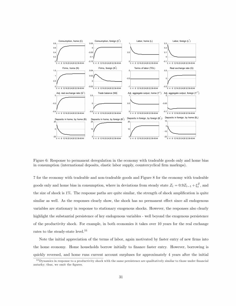
0 4 8 1216 20 2428 32 36 40440

0.2

0.4

0.6

0.8Consumption, home (C)

0 4 8 1216 20 2428 32 36 4044-0.15

-0.1

-0.05

0

0.05Consumption, foreign (C*)

0 4 8 1216 20 2428 32 36 40440

0.5

1Labor, home (L)

0 4 8 1216 20 2428 32 36 4044-0.1

0

0.1

0.2

0.3Labor, foreign (L*)

0 4 8 1216 20 2428 32 36 40440

0.5

1

1.5Firms, home (N)

0 4 8 1216 20 2428 32 36 4044-0.02

0

0.02

0.04Firms, foreign (N*)

0 4 8 1216 20 2428 32 36 4044-1

-0.5

0Terms of labor (TOL)

0 4 8 1216 20 2428 32 36 4044-0.5

0

0.5Real exchange rate (Q)

0 4 8 1216 20 2428 32 36 4044-0.4

-0.2

0Adj. real exchange rate (Q~)

0 4 8 1216 20 2428 32 36 4044-0.5

0

0.5Trade balance (NX)

0 4 8 1216 20 2428 32 36 40440

0.5

1Adj. aggregate output, home (Y~)

0 4 8 1216 20 2428 32 36 4044-0.1

-0.05

0Adj. aggregate output, foreign (Y~*)

0 4 8 1216 20 2428 32 36 4044-20

0

20Deposits in home, by home (B)

0 4 8 1216 20 2428 32 36 40440

10

20Deposits in home, by foreign (B*)

0 4 8 1216 20 2428 32 36 40440

10

20

Deposits in foreign, by foreign (B**)

0 4 8 1216 20 2428 32 36 4044-20

-10

0

10

Deposits in foreign, by home (B*)

Figure 6: Response to permanent deregulation in the economy with tradeable goods only and home biasin consumption (international deposits, elastic labor supply, countercyclical firm markups).

7 for the economy with tradeable and non-tradeable goods and Figure 8 for the economy with tradeable

goods only and home bias in consumption, where in deviations from steady state Zt = 0.9Zt−1+ ξZt , and

the size of shock is 1%. The response paths are quite similar, the strength of shock amplification is quite

similar as well. As the responses clearly show, the shock has no permanent effect since all endogenous

variables are stationary in response to stationary exogenous shocks. However, the responses also clearly

highlight the substantial persistence of key endogenous variables - well beyond the exogenous persistence

of the productivity shock. For example, in both economies it takes over 10 years for the real exchange

rates to the steady-state level.33

Note the initial appreciation of the terms of labor, again motivated by faster entry of new firms into

the home economy. Home households borrow initially to finance faster entry. However, borrowing is

quickly reversed, and home runs current account surpluses for approximately 4 years after the initial33Dynamics in response to a productivity shock with the same persistence are qualitatively similar to those under financial

autarky; thus, we omit the figures.

31

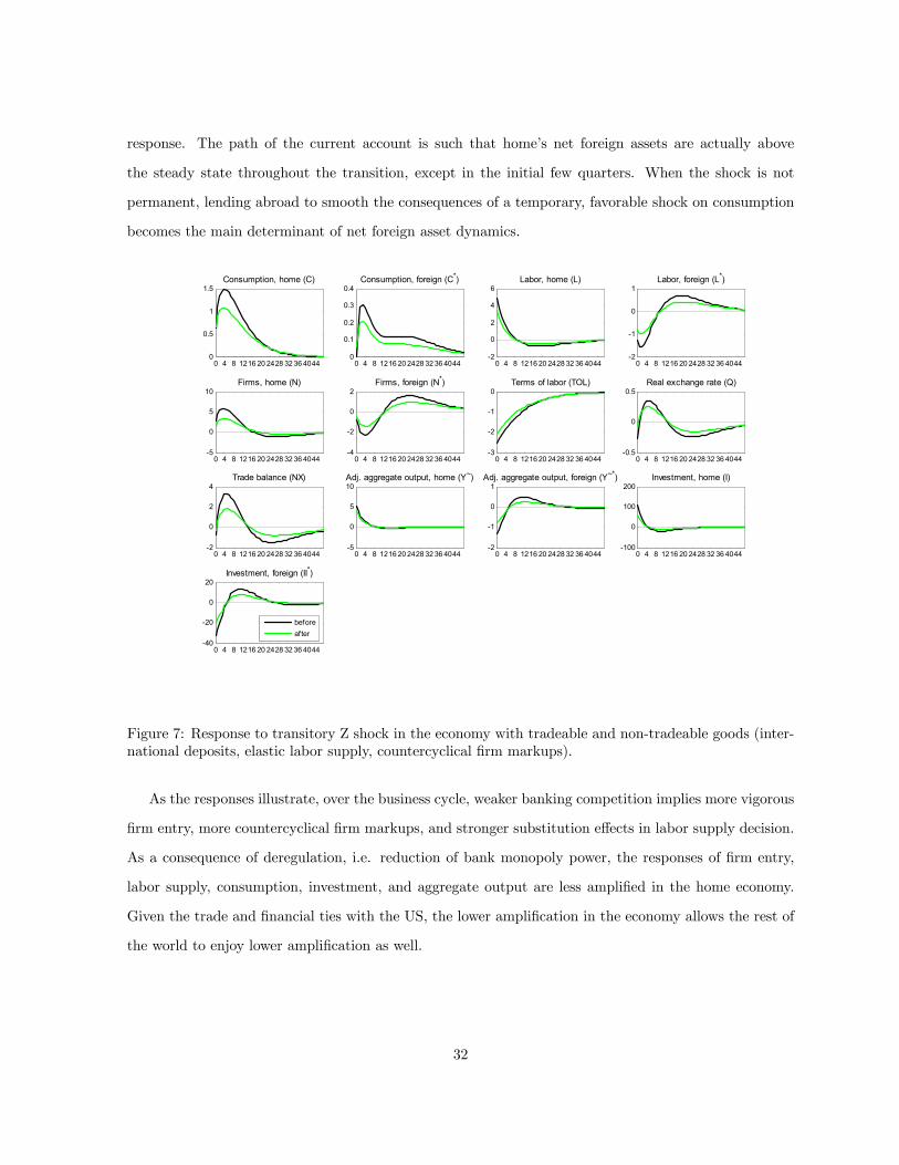
response. The path of the current account is such that home’s net foreign assets are actually above

the steady state throughout the transition, except in the initial few quarters. When the shock is not

permanent, lending abroad to smooth the consequences of a temporary, favorable shock on consumption

becomes the main determinant of net foreign asset dynamics.

0 4 8 1216 20 2428 32 36 40440

0.5

1

1.5Consumption, home (C)

0 4 8 1216 20 2428 32 36 40440

0.1

0.2

0.3

0.4Consumption, foreign (C*)

0 4 8 1216 20 2428 32 36 4044-2

0

2

4

6Labor, home (L)

0 4 8 1216 20 2428 32 36 4044-2

-1

0

1Labor, foreign (L*)

0 4 8 1216 20 2428 32 36 4044-5

0

5

10Firms, home (N)

0 4 8 1216 20 2428 32 36 4044-4

-2

0

2Firms, foreign (N*)

0 4 8 1216 20 2428 32 36 4044-3

-2

-1

0Terms of labor (TOL)

0 4 8 1216 20 2428 32 36 4044-0.5

0

0.5Real exchange rate (Q)

0 4 8 1216 20 2428 32 36 4044-2

0

2

4Trade balance (NX)

0 4 8 1216 20 2428 32 36 4044-5

0

5

10Adj. aggregate output, home (Y~)

0 4 8 1216 20 2428 32 36 4044-2

-1

0

1Adj. aggregate output, foreign (Y~*)

0 4 8 1216 20 2428 32 36 4044-100

0

100

200Investment, home (I)

0 4 8 1216 20 2428 32 36 4044-40

-20

0

20Investment, foreign (II*)

beforeafter

Figure 7: Response to transitory Z shock in the economy with tradeable and non-tradeable goods (inter-national deposits, elastic labor supply, countercyclical firm markups).

As the responses illustrate, over the business cycle, weaker banking competition implies more vigorous

firm entry, more countercyclical firm markups, and stronger substitution effects in labor supply decision.

As a consequence of deregulation, i.e. reduction of bank monopoly power, the responses of firm entry,

labor supply, consumption, investment, and aggregate output are less amplified in the home economy.

Given the trade and financial ties with the US, the lower amplification in the economy allows the rest of

the world to enjoy lower amplification as well.

32

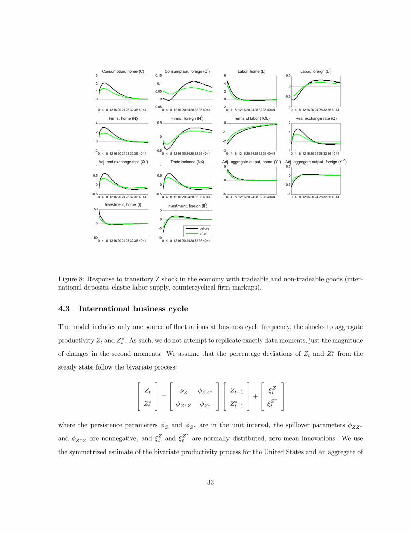
0 4 8 1216 20 2428 32 36 4044-1

0

1

2

3Consumption, home (C)

0 4 8 1216 20 2428 32 36 4044-0.05

0

0.05

0.1

0.15Consumption, foreign (C*)

0 4 8 1216 20 2428 32 36 4044-2

0

2

4

6Labor, home (L)

0 4 8 1216 20 2428 32 36 4044-1

-0.5

0

0.5Labor, foreign (L*)

0 4 8 1216 20 2428 32 36 4044-2

0

2

4Firms, home (N)

0 4 8 1216 20 2428 32 36 4044-0.5

0

0.5Firms, foreign (N*)

0 4 8 1216 20 2428 32 36 4044-3

-2

-1

0Terms of labor (TOL)

0 4 8 1216 20 2428 32 36 4044-1

0

1

2Real exchange rate (Q)

0 4 8 1216 20 2428 32 36 4044-0.5

0

0.5

1Adj. real exchange rate (Q~)

0 4 8 1216 20 2428 32 36 4044-0.5

0

0.5

1Trade balance (NX)

0 4 8 1216 20 2428 32 36 4044-5

0

5Adj. aggregate output, home (Y~)

0 4 8 1216 20 2428 32 36 4044-1

-0.5

0

0.5Adj. aggregate output, foreign (Y~*)

0 4 8 1216 20 2428 32 36 4044-50

0

50Investment, home (I)

0 4 8 1216 20 2428 32 36 4044-10

-5

0

5Investment, foreign (II*)

beforeafter

Figure 8: Response to transitory Z shock in the economy with tradeable and non-tradeable goods (inter-national deposits, elastic labor supply, countercyclical firm markups).

4.3 International business cycle

The model includes only one source of fluctuations at business cycle frequency, the shocks to aggregate

productivity Zt and Z∗t . As such, we do not attempt to replicate exactly data moments, just the magnitude

of changes in the second moments. We assume that the percentage deviations of Zt and Z∗t from the

steady state follow the bivariate process:

Zt

Z∗t

= φZ φZZ∗

φZ∗Z φZ∗

Zt−1

Z∗t−1

+ ξZt

ξZ∗

t

where the persistence parameters φZ and φZ∗ are in the unit interval, the spillover parameters φZZ∗

and φZ∗Z are nonnegative, and ξZt and ξZ∗

t are normally distributed, zero-mean innovations. We use

the symmetrized estimate of the bivariate productivity process for the United States and an aggregate of

33

European economies in Backus et al (1992) and set

φZ φZZ∗

φZ∗Z φZ∗

= 0.906 0.088

0.088 0.906

.This matrix implies a small, positive productivity spillover across countries, such that, if home pro-

ductivity rises during period t, foreign productivity will also increase at t + 1. We set the standard

deviation of the productivity innovations to.1% and the correlation to 0.258 (corresponding to a 0.19

percent covariance), the latter as estimated by Backus et al. We calculate the implied second moments of

endogenous variables (percent deviations from steady state) using the frequency domain technique. We

focus on the high-frequency properties of business cycles in home and foreign, we report second moments

of Hodrick-Prescott (HP)-filtered variables.

We previously noted that empirical price deflators are best represented by the average prices ePt andeP ∗t in our model (as opposed to the welfare based price indices Pt and P ∗t ). Thus, we focus on the secondmoments of real variables deflated by the average prices ePt and eP ∗t . As we previously discussed, newentrants embody the investment by households, and the stock of firms represents the capital accumulated

by such investments. For comparison with the investment and capital variables in standard models, we

compute second moments for nt and n∗t as well as for investment in new firms deflated by the average

price.eIt = wt/ZtntPt/ ePt and eI∗t = w∗t /Z∗t n∗tP ∗t / eP ∗t .Table 4 reports standard deviations for the economy with tradeable and non-tradeable goods and for

the economy with tradeable goods only and home bias in consumption. Both models are successful at

generating less volatile consumption than GDP, labor volatile (roughly) as GDP, more volatile investment

than GDP. However, both models overpredict the ratio of standard deviations of firm entry (and invest-

ment) to aggregate output; in the data this ratio lies between 3 and 4. Both models are also successful at

generating significant volatility reduction after deregulation in home country comparable in magnitude

with that observed in the data for the US. Over the business cycle, weaker banking competition implies

more vigorous firm entry, more countercyclical firm markups, and stronger substitution effects in labor

supply decision. As a consequence of deregulation, firm entry, labor supply, consumption, investment,

and aggregate output are all less volatile in the US. The trade and financial ties with the US allow the

rest of the world to enjoy lower volatility as well.

Table 5 reports variance decomposition for the economy with tradeable and non-tradeable goods

34

Table 4: Standard deviations (in percent, HP filtered)

Economy with tradeable Economy with tradeable goods onlyand non-tradeable goods and home bias in consumptionBefore After Change,%

C 1.6296 1.2791 −21.51C∗ 1.6296 1.5906 −2.40L 6.5460 5.5095 −15.83L∗ 6.5460 5.6558 −13.60n 140.4298 94.5894 −32.64n∗ 140.4297 121.7101 −13.33TOL 2.9906 2.5778 −13.80Q ( eQ) 1.0705 0.8402 −21.51NX 8.0399 5.7781 −28.13eY 6.1438 5.3642 −12.69eY ∗ 6.1438 5.5426 −9.79eI 140.4330 94.5795 −32.65eI∗ 140.4329 121.6827 −13.3517

Before After Change,%C 2.1425 1.5347 −28.37C∗ 2.1425 2.1031 −1.84L 5.4454 4.4762 −17.80L∗ 5.4454 5.1529 −5.37n 51.1245 34.6967 −32.13n∗ 51.1245 48.4664 −5.20TOL 2.7220 2.3122 −15.06Q 2.6411 2.0594 −22.02eQ 1.3441 1.0328 −23.16NX 1.4021 1.0797 −23.00eY 4.5082 3.9459 −12.47eY ∗ 4.5082 4.3585 −3.32eI 51.0484 34.6388 −32.1452eI∗ 51.0484 48.3826 −5.2220

and for the economy with tradeable goods only and home bias in consumption. Both models predict

a (slight) increase in importance of the shocks originated in the rest of the world after deregulation for

home aggregate output, investment, and labor supply, but for consumption.

5 Conclusion

We developed a two-country model of the domestic and external effects of financial deregulation that pre-

dicts real appreciation, external borrowing, and moderation of domestic and international business cycles

as joint equilibrium consequences of increased competition in banking in the country that deregulates.

The key channel through which this occurs is an increase in the attractiveness of this country’s business

environment relative to the rest of the world. The model provides a unified explanation of features of

behavior of the U.S. and international economy following the drastic deregulation of U.S. banking started

in 1977 and finalized in 1994.

Our paper thus contributes to a growing body of literature on observed dynamics of external balances,

business cycles, and international relative prices. It provides a complementary explanation of equilibrium

external imbalances that highlights an additional source of cross-country asymmetry in the characteristics

of financial sectors relative to those emphasized by Caballero et al (2006) and Mendoza et al (2007). It

35

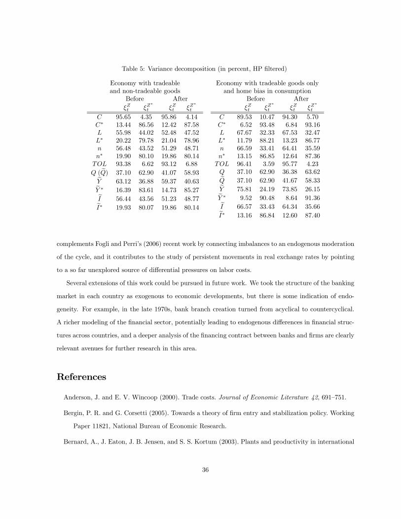
Table 5: Variance decomposition (in percent, HP filtered)

Economy with tradeable Economy with tradeable goods onlyand non-tradeable goods and home bias in consumption

Before AfterξZt ξZ

∗t ξZt ξZ

∗t

C 95.65 4.35 95.86 4.14C∗ 13.44 86.56 12.42 87.58L 55.98 44.02 52.48 47.52L∗ 20.22 79.78 21.04 78.96n 56.48 43.52 51.29 48.71n∗ 19.90 80.10 19.86 80.14TOL 93.38 6.62 93.12 6.88

Q ( eQ) 37.10 62.90 41.07 58.93eY 63.12 36.88 59.37 40.63eY ∗ 16.39 83.61 14.73 85.27eI 56.44 43.56 51.23 48.77eI∗ 19.93 80.07 19.86 80.14

Before AfterξZt ξZ

∗t ξZt ξZ

∗t

C 89.53 10.47 94.30 5.70C∗ 6.52 93.48 6.84 93.16L 67.67 32.33 67.53 32.47L∗ 11.79 88.21 13.23 86.77n 66.59 33.41 64.41 35.59n∗ 13.15 86.85 12.64 87.36TOL 96.41 3.59 95.77 4.23Q 37.10 62.90 36.38 63.62eQ 37.10 62.90 41.67 58.33eY 75.81 24.19 73.85 26.15eY ∗ 9.52 90.48 8.64 91.36eI 66.57 33.43 64.34 35.66eI∗ 13.16 86.84 12.60 87.40

complements Fogli and Perri’s (2006) recent work by connecting imbalances to an endogenous moderation

of the cycle, and it contributes to the study of persistent movements in real exchange rates by pointing

to a so far unexplored source of differential pressures on labor costs.

Several extensions of this work could be pursued in future work. We took the structure of the banking

market in each country as exogenous to economic developments, but there is some indication of endo-

geneity. For example, in the late 1970s, bank branch creation turned from acyclical to countercyclical.

A richer modeling of the financial sector, potentially leading to endogenous differences in financial struc-

tures across countries, and a deeper analysis of the financing contract between banks and firms are clearly

relevant avenues for further research in this area.

References

Anderson, J. and E. V. Wincoop (2000). Trade costs. Journal of Economic Literature 42, 691—751.

Bergin, P. R. and G. Corsetti (2005). Towards a theory of firm entry and stabilization policy. Working

Paper 11821, National Bureau of Economic Research.

Bernard, A., J. Eaton, J. B. Jensen, and S. S. Kortum (2003). Plants and productivity in international

36

trade. American Economic Review 93 (4), 1268—1290.

Bilbiie, F., F. Ghironi, and M. Melitz (2008). Monetary policy and business cycles with endogenous

entry and product variety (forthcoming). In D. Acemoglu, K. S. Rogoff, and M. Woodford (Eds.),

NBER Macroeconomics Annual 2007, Cambridge, MA. MIT Press.

Bilbiie, F., F. Ghironi, and M. J. Melitz (2005). Endogenous entry, product variety, and business cycles.

Working paper, Boston College.

Black, S. E. and P. E. Strahan (2002). Entrepreneurship and bank credit availability. Journal of Fi-

nance 57 (6), 2807—2833.

Caballero, R. J. (2006). On the macroeconomics of asset shortages. NBER Working Paper 12753,

National Bureau of Economic Research.

Caballero, R. J., E. Farhi, and P.-O. Gourinchas (2006). An equilibrium model of ”global imbalances”

and low interest rates. NBER Working Paper 11996, National Bureau of Economic Research.

Cestone, G. and L. White (2003). Anticompetitive financial contracting: The design of financial claims.

Journal of Finance 58 (5), 2109—2142.

Cetorelli, N. and P. E. Strahan (2006). Finance as a barrier to entry: Bank competition and industry

structure in local U.S. markets. Journal of Finance 61 (1), 437—461.

Comin, D. and M. Gertler (2006). Medium term business cycles. American Economic Review 96 (3),

523—551.

Corsetti, G., P. Martin, and P. Pesenti (2007a). Productivity, terms of trade and the "home market

effect". Journal of International Economics 73 (1), 99—127.

Corsetti, G., P. Martin, and P. Pesenti (2007b). Varieties and the transfer problem: The extensive

margin of current account adjustment. Manuscript, European University Institute.

D’Aspremont, C., R. D. S. Ferreira, and L.-A. Gerard-Varet (1996). On the Dixit-Stiglitz model of

monopolistic competition. American Economic Review 86 (3), 623—629.

Davis, S. J., J. C. Haltiwanger, R. Jarmin, and J. Miranda (2006). Volatility and dispersion in business

growth rates: Publicly traded versus privately held firms. NBER Working Paper 12354, National

Bureau of Economic Research.

37

DeBandt, O. and E. P. Davis (2000). Competition, contestability and market structure in european

banking sectors on the eve of emu. Journal of Banking and Finance 24 (6), 1045—1066(22).

Elkhoury, M. and T. Mancini-Griffoli (2006). Monetary policy with firm entry. Manuscript, Graduate

Institute of International Studies, Geneva.

Erceg, C. J., L. Guerrieri, and C. J. Gust (2005). Expansionary fiscal shocks and the trade deficit.

International Finance 8 (3), 363—397.

Fogli, A. and F. Perri (2006). The ”great moderation” and the us external imbalance. NBERWorking

Paper 12708, National Bureau of Economic Research.

Ghironi, F. and M. Melitz (2007). Trade flow dynamics with heterogeneous firms. American Economic

Review (Papers and Proceedings) 97 (2), 356—361.

Ghironi, F. and M. J. Melitz (2005). International trade and macroeconomic dynamics with heteroge-

neous firms. Quarterly Journal of Economics 120 (3), 865—915.

González-Maestre, M. and L. M. Granero (2003). Industrial loans and market structure. European

Economic Review 47 (5), 841—55.

Hunt, B. and A. Rebucci (2005). The us dollar and the trade deficit: What accounts for the late 1990s?

International Finance 8 (3), 399—434.

Jaimovich, N. (2006). Firm dynamics, markup variations and the business cycle. Working paper, Stan-

ford University.

King, R. G., C. I. Plosser, and S. T. Rebelo (1988). Production, growth and business cycles: I. The

basic neoclassical model. Journal of Monetary Economics 21 (2-3), 195—232.

Lewis, V. (2006). Macroeconomic fluctuations and firm entry: Theory and evidence. Working Paper

103, National Bank of Belgium.

Mendoza, E. G., V. Quadrini, and J.-V. Rios-Rull (2007). Financial integration, financial deepness and

global imbalances. NBER Working Paper 12909, National Bureau of Economic Research.

Méjean, I. (2007). Can firms’ location decisions counteract the balassa-samuelson effect? Manuscript,

CEPII, Paris.

Stebunovs, V. (2006). Finance as a barrier to entry: U.S. bank deregulation and volatility. Job market

paper, Boston College.

38

Woodford, M. (2003). Interest and Prices: Foundations of a Theory of Monetary Policy. Princeton,

NJ: Princeton University Press.

Yang, X. and B. J. Heijdra (1993). Monopolistic competition and optimum product diversity: Com-

ment. American Economic Review 83 (1), 295—301.

39

6 Appendix

6.1 International deposits

The budget constraint of the representative home household, in units of the home consumption basket,

is now

Bt+QtB∗,t+η

2

£B2t +QtB

2∗,t¤+vtxt+1+Ct = (1+rt−1)Bt−1+Qt(1+r∗t−1)B∗,t−1+(πt+vt)xt+T

Ft +wtl,

where Bt denotes holdings of home deposits, B∗,t denotes holdings of foreign deposits, η2B

2t is the cost

of adjusting holdings of home deposits, η2QtB

2∗,t is the cost of adjusting holdings of foreign deposits

(in units of foreign consumption), TFt is the fee rebate, taken as given by the household, and equal to

η2

£B2t +QtB∗,t2

¤in equilibrium. For simplicity, we assume that the scale parameter η > 0 is identical

across costs of adjusting holdings of home and foreign deposits. Also, there is no cost of adjusting equity

holdings. Hence, in equilibrium, deposit - adjustment fees capture fees on international transactions,

which we assume absent from domestic transactions such as those involving equity to avoid adding

unnecessary complication. The representative foreign household faces a similar constraint, in units of

foreign consumption.

Home and foreign households maximize the respective intertemporal utility functions subject to the

respective constraints. The first-order conditions for the choices of share holdings in mutual portfolios

of domestic firms at home and abroad are unchanged relative to the case of financial autarky. The new

Euler equations for home and foreign deposit holdings, deposit market clearing condition, bank profit,

replace the equations in Table 1. Since trade is no longer balanced under international deposit trading,

we must explicitly impose labor market clearing conditions in both countries. To close the model we add

the net foreign asset equation. Aggregate accounting implies the law of motion for net foreign assets at

home

Bt +QtB∗,t =£Qt(1 + r

∗t−1)B∗,t−1 − (1 + rt−1)B∗t−1

¤+ dtNt + wtL− Ct,

where holdings of individual deposits across countries are tied by the equilibrium condition Bt + B∗t =

wtZtnt. Similar equations hold abroad. Given these conditions, multiplying the law of motion for net

foreign assets at foreign times Qt and subtracting the resulting equation from the law of motion for

net foreign assets at home yields an expression for the difference of home and foreign net foreign asset

40

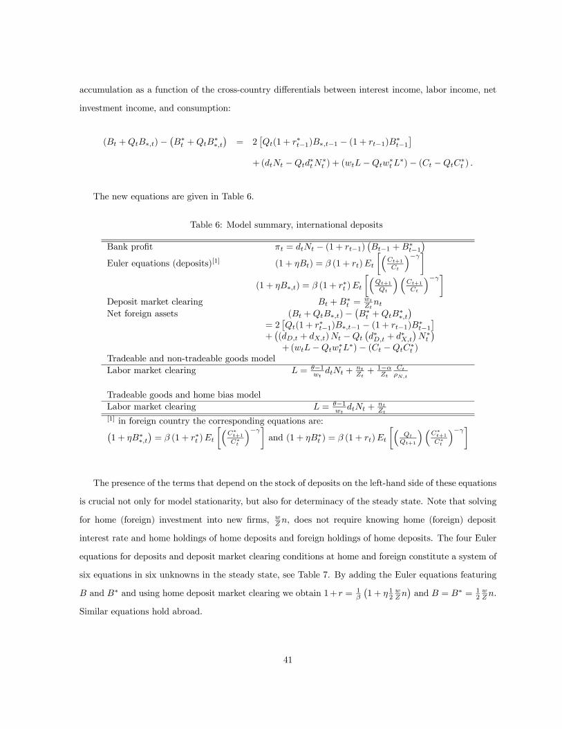
accumulation as a function of the cross-country differentials between interest income, labor income, net

investment income, and consumption:

(Bt +QtB∗,t)−¡B∗t +QtB

∗∗,t¢= 2

£Qt(1 + r

∗t−1)B∗,t−1 − (1 + rt−1)B∗t−1

¤+(dtNt −Qtd∗tN∗t ) + (wtL−Qtw∗tL∗)− (Ct −QtC∗t ) .

The new equations are given in Table 6.

Table 6: Model summary, international deposits

Bank profit πt = dtNt − (1 + rt−1)¡Bt−1 +B∗t−1

¢Euler equations (deposits)[1] (1 + ηBt) = β (1 + rt)Et

·³Ct+1Ct

´−γ¸(1 + ηB∗,t) = β (1 + r∗t )Et

·³Qt+1

Qt

´³Ct+1Ct

´−γ¸Deposit market clearing Bt +B

∗t =

wtZtnt

Net foreign assets (Bt +QtB∗,t)−¡B∗t +QtB

∗∗,t¢

= 2£Qt(1 + r

∗t−1)B∗,t−1 − (1 + rt−1)B∗t−1

¤+¡(dD,t + dX,t)Nt −Qt

¡d∗D,t + d

∗X,t

¢N∗t¢

+(wtL−Qtw∗tL∗)− (Ct −QtC∗t )Tradeable and non-tradeable goods modelLabor market clearing L = θ−1

wtdtNt +

ntZt+ 1−α

ZtCtρN,t

Tradeable goods and home bias modelLabor market clearing L = θ−1

wtdtNt +

ntZt

[1] in foreign country the corresponding equations are:¡1 + ηB∗∗,t

¢= β (1 + r∗t )Et

·³C∗t+1C∗t

´−γ¸and (1 + ηB∗t ) = β (1 + rt)Et

·³Qt

Qt+1

´³C∗t+1C∗t

´−γ¸

The presence of the terms that depend on the stock of deposits on the left-hand side of these equations

is crucial not only for model stationarity, but also for determinacy of the steady state. Note that solving

for home (foreign) investment into new firms, wZn, does not require knowing home (foreign) deposit

interest rate and home holdings of home deposits and foreign holdings of home deposits. The four Euler

equations for deposits and deposit market clearing conditions at home and foreign constitute a system of

six equations in six unknowns in the steady state, see Table 7. By adding the Euler equations featuring

B and B∗ and using home deposit market clearing we obtain 1+ r = 1β

¡1 + η 12

wZn¢and B = B∗ = 1

2wZn.

Similar equations hold abroad.

41

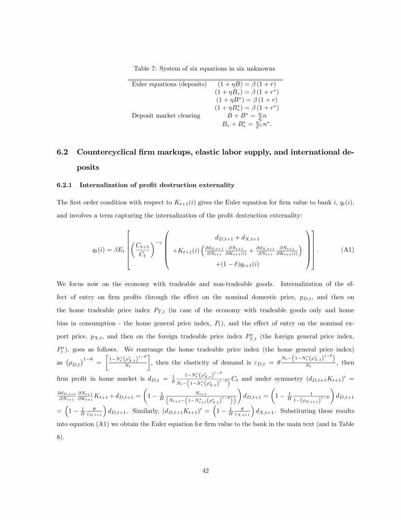
Table 7: System of six equations in six unknowns

Euler equations (deposits) (1 + ηB) = β (1 + r)(1 + ηB∗) = β (1 + r∗)(1 + ηB∗) = β (1 + r)(1 + ηB∗∗) = β (1 + r∗)

Deposit market clearing B +B∗ = wZn

B∗ +B∗∗ =w∗Z∗n

∗.

6.2 Countercyclical firm markups, elastic labor supply, and international de-

posits

6.2.1 Internalization of profit destruction externality

The first order condition with respect to Kt+1(i) gives the Euler equation for firm value to bank i, qt(i),

and involves a term capturing the internalization of the profit destruction externality:

qt(i) = βEt

µCt+1Ct

¶−γ

dD,t+1 + dX,t+1

+Kt+1(i)³∂dD,t+1

∂Nt+1

∂Nt+1

∂Kt+1(i)+

∂dX,t+1∂Nt+1

∂Nt+1

∂Kt+1(i)

´+(1− δ)qt+1(i)

. (A1)

We focus now on the economy with tradeable and non-tradeable goods. Internalization of the ef-

fect of entry on firm profits through the effect on the nominal domestic price, pD,t, and then on

the home tradeable price index PT,t (in case of the economy with tradeable goods only and home

bias in consumption - the home general price index, Pt), and the effect of entry on the nominal ex-

port price, pX,t, and then on the foreign tradeable price index P ∗T,t (the foreign general price index,

P ∗t ), goes as follows. We rearrange the home tradeable price index (the home general price index)

as¡ρD,t

¢1−θ=

·1−N∗t (ρ∗X,t)

1−θ

Nt

¸, then the elasticity of demand is εD,t = θ

Nt−³1−N∗t (ρ∗X,t)

1−θ´Nt

, then

firm profit in home market is dD,t = 1θ

1−N∗t (ρ∗X,t)1−θ

Nt−³1−N∗t (ρ∗X,t)

1−θ´Ct and under symmetry (dD,t+1Kt+1)0 =∂dD,t+1

∂Nt+1

∂Nt+1

∂Kt+1Kt+1+ dD,t+1 =

µ1− 1

HNt+1³

Nt+1−³1−N∗t+1(ρ∗X,t)

1−θ´´¶dD,t+1 =

µ1− 1

H1

1−(ρD,t+1)1−θ

¶dD,t+1

=³1− 1

Hθ

εD,t+1

´dD,t+1. Similarly, (dD,t+1Kt+1)0 =

³1− 1

Hθ

εX,t+1

´dX,t+1. Substituting these results

into equation (A1) we obtain the Euler equation for firm value to the bank in the main text (and in Table

8).

42

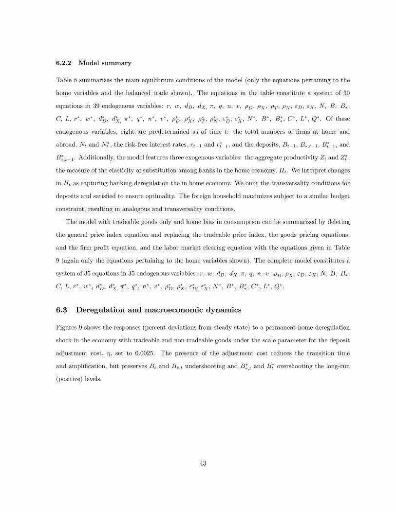
6.2.2 Model summary

Table 8 summarizes the main equilibrium conditions of the model (only the equations pertaining to the

home variables and the balanced trade shown). The equations in the table constitute a system of 39

equations in 39 endogenous variables: r, w, dD, dX, π, q, n, v, ρD, ρX , ρT , ρN , εD, εX , N, B, B∗,

C, L, r∗, w∗, d∗D, d∗X, π

∗, q∗, n∗, v∗, ρ∗D, ρ∗X , ρ

∗T , ρ

∗N , ε

∗D, ε

∗X , N

∗, B∗, B∗∗ , C∗, L∗, Q∗. Of these

endogenous variables, eight are predetermined as of time t: the total numbers of firms at home and

abroad, Nt and N∗t , the risk-free interest rates, rt−1 and r∗t−1, and the deposits, Bt−1, B∗,t−1, B

∗t−1, and

B∗∗,t−1. Additionally, the model features three exogenous variables: the aggregate productivity Zt and Z∗t ,

the measure of the elasticity of substitution among banks in the home economy, Ht. We interpret changes

in Ht as capturing banking deregulation the in home economy. We omit the transversality conditions for

deposits and satisfied to ensure optimality. The foreign household maximizes subject to a similar budget

constraint, resulting in analogous and transversality conditions.

The model with tradeable goods only and home bias in consumption can be summarized by deleting

the general price index equation and replacing the tradeable price index, the goods pricing equations,

and the firm profit equation, and the labor market clearing equation with the equations given in Table

9 (again only the equations pertaining to the home variables shown). The complete model constitutes a

system of 35 equations in 35 endogenous variables: r, w, dD, dX, π, q, n, v, ρD, ρX , εD, εX , N, B, B∗,

C, L, r∗, w∗, d∗D, d∗X, π

∗, q∗, n∗, v∗, ρ∗D, ρ∗X , ε

∗D, ε

∗X , N

∗, B∗, B∗∗ , C∗, L∗, Q∗.

6.3 Deregulation and macroeconomic dynamics

Figures 9 shows the responses (percent deviations from steady state) to a permanent home deregulation

shock in the economy with tradeable and non-tradeable goods under the scale parameter for the deposit

adjustment cost, η, set to 0.0025. The presence of the adjustment cost reduces the transition time

and amplification, but preserves Bt and B∗,t undershooting and B∗∗,t and B∗t overshooting the long-run

(positive) levels.

43

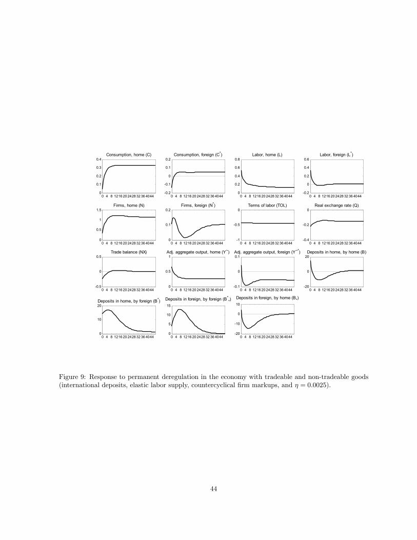
0 4 8 1216 20 2428 32 36 40440

0.1

0.2

0.3

0.4Consumption, home (C)

0 4 8 1216 20 2428 32 36 4044-0.2

-0.1

0

0.1

0.2Consumption, foreign (C*)

0 4 8 1216 20 2428 32 36 40440

0.2

0.4

0.6

0.8Labor, home (L)

0 4 8 1216 20 2428 32 36 4044-0.2

0

0.2

0.4

0.6Labor, foreign (L*)

0 4 8 1216 20 2428 32 36 40440

0.5

1

1.5Firms, home (N)

0 4 8 1216 20 2428 32 36 40440

0.1

0.2Firms, foreign (N*)

0 4 8 1216 20 2428 32 36 4044-1

-0.5

0Terms of labor (TOL)

0 4 8 1216 20 2428 32 36 4044-0.4

-0.2

0Real exchange rate (Q)

0 4 8 1216 20 2428 32 36 4044-0.5

0

0.5Trade balance (NX)

0 4 8 1216 20 2428 32 36 40440

0.5

1Adj. aggregate output, home (Y~)

0 4 8 1216 20 2428 32 36 4044-0.1

0

0.1Adj. aggregate output, foreign (Y~*)

0 4 8 1216 20 2428 32 36 4044-20

0

20Deposits in home, by home (B)

0 4 8 1216 20 2428 32 36 40440

10

20Deposits in home, by foreign (B*)

0 4 8 1216 20 2428 32 36 40440

5

10

15

Deposits in foreign, by foreign (B**)

0 4 8 1216 20 2428 32 36 4044-20

-10

0

10

Deposits in foreign, by home (B*)

Figure 9: Response to permanent deregulation in the economy with tradeable and non-tradeable goods(international deposits, elastic labor supply, countercyclical firm markups, and η = 0.0025).

44

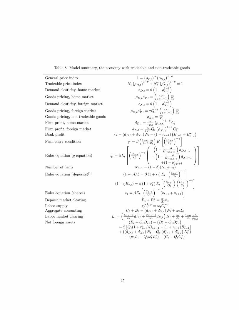
Table 8: Model summary, the economy with tradeable and non-tradeable goods

General price index 1 =¡ρT,t

¢α ¡ρN,t

¢1−αTradeable price index Nt

¡ρD,t

¢1−θ+N∗t

¡ρ∗X,t

¢1−θ= 1

Demand elasticity, home market εD,t = θ³1− ρ1−θD,t

´Goods pricing, home market ρD,tρT,t =

³εD,t

εD,t−1´wtZt

Demand elasticity, foreign market εX,t = θ³1− ρ1−θX,t

´Goods pricing, foreign market ρX,tρ

∗T,t = τQ−1t

³εX,t

εX,t−1´wtZt

Goods pricing, non-tradeable goods ρN,t =wtZt

Firm profit, home market dD,t =α

εD,t

¡ρD,t

¢1−θCt

Firm profit, foreign market dX,t =α

εX,tQt¡ρX,t

¢1−θC∗t

Bank profit πt = (dD,t + dX,t)Nt − (1 + rt−1)¡Bt−1 +B∗t−1

¢Firm entry condition qt = β

³1+rt1−δ

wtZt

´Et

·³Ct+1Ct

´−γ¸

Euler equation (q equation) qt = βEt

³Ct+1Ct

´−γ³1− 1

Hθ

εD,t+1

´dD,t+1

+³1− 1

Hθ

εX,t+1

´dX,t+1

+(1− δ)qt+1

Number of firms Nt+1 = (1− δ)(Nt + nt)

Euler equation (deposits)[1] (1 + ηBt) = β (1 + rt)Et

·³Ct+1Ct

´−γ¸(1 + ηB∗,t) = β (1 + r∗t )Et

·³Qt+1

Qt

´³Ct+1Ct

´−γ¸Euler equation (shares) vt = βEt

·³Ct+1Ct

´−γ(vt+1 + πt+1)

¸Deposit market clearing Bt +B

∗t =

wtZtnt

Labor supply χL1/ϕt = wtC

−γt

Aggregate accounting Ct +Bt = (dD,t + dX,t)Nt + wtLt

Labor market clearing Lt =³εD,t−1wt

dD,t +εX,t−1wt

dX,t

´Nt +

ntZt+ 1−α

ZtCtρN,t

Net foreign assets (Bt +QtB∗,t)−¡B∗t +QtB∗∗,t

¢= 2

£Qt(1 + r

∗t−1)B∗,t−1 − (1 + rt−1)B∗t−1

¤+¡(dD,t + dX,t)Nt −Qt

¡d∗D,t + d

∗X,t

¢N∗t¢

+(wtLt −Qtw∗tL∗t )− (Ct −QtC∗t )

45

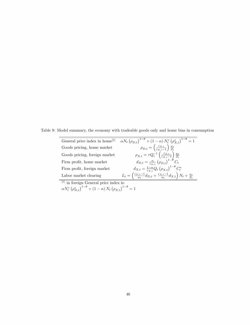
Table 9: Model summary, the economy with tradeable goods only and home bias in consumption

General price index in home[1] αNt¡ρD,t

¢1−θ+ (1− α)N∗t

¡ρ∗X,t

¢1−θ= 1

Goods pricing, home market ρD,t =³

εD,t

εD,t−1´wtZt

Goods pricing, foreign market ρX,t = τQ−1t³

εX,tεX,t−1

´wtZt

Firm profit, home market dD,t =α

εD,t

¡ρD,t

¢1−θCt

Firm profit, foreign market dX,t =1−αεX,t

Qt¡ρX,t

¢1−θC∗t

Labor market clearing Lt =³εD,t−1wt

dD,t +εX,t−1wt

dX,t

´Nt +

ntZt

[1] in foreign General price index is:

αN∗t¡ρ∗D,t

¢1−θ+ (1− α)Nt

¡ρX,t

¢1−θ= 1

46