The Doubtful Profitability of Foggy Pricing?

Eugenio J. Miravete†

September 20, 2007

Abstract

A particular tariff option is said to be foggy when another option or a combination of other tariff optionsoffered by the same firm is always less expensive regardless of the usage profile of any customer. Alterna-tively, tariff fogginess may be referred to the whole set of tariff options and it is related to the low likelihoodthat a particular tariff option ends up being the least expensive one among those of a menu of tariff plansfor an arbitrary distribution of usage patterns. This paper takes advantage of the exogenous entry of asecond carrier in the early U.S. cellular telephone industry. It shows that competition induces firms tointroduce mostly non-foggy options, thus abandoning deceptive pricing strategies (fog lifting) aimed toprofit from mistaken choices of consumers rather than softening competition through the use of foggytactics (co-opetition). Results indicate that tariff fogginess becomes less severe with the entry of a secondfirm in the industry. Thus competition appears to correct deceptive pricing strategies while at the sametime increases the total number of tariffs offered to consumers. Still, such correction of deceptive strategiesoccurs only in the long run rather than immediately after the entry of a second firm. Results are robustto the existence of individual uncertainty regarding future telephone usage when consumers sign up for aparticular tariff plan.

Keywords: Nonlinear Pricing; Foggy Strategies; Co-opetition; Fog Lifting; Phasing-out.

JEL Codes: D43, L96, M21

?The NET Institute (http://www.NETinst.org) offered generous financial support through its 2004 Summer Grant Program.

I thank seminar audiences at Haas School of Business (Berkeley), IESE, ITAM, Wharton, the 2006 CEPR Conference on AppliedIndustrial Organization held in Madeira, and the 2007 Meeting of the New Zealand Association of Economists held in Christchurch. Iparticularly thank Barry Nalebuff for his critical disagreement on the empirical approach I took in a much earlier version of this paper.Trying to accommodate his comments prompted me to search for additional data and forced me to look for better ways to exploit thetariff information that was already available to me. This is true in particular for dealing with the phasing-out of tariffs. Evidently, Iam solely responsible for all errors that might still remain.

†The University of Texas at Austin, Department of Economics, BRB 1.116, 1 University Station C3100, Austin, Texas 78712-0301; S.T. Lee Visiting Fellow, Institute for the Study of Competition and Regulation, Wellington, New Zealand; and CEPR, London,UK. Phone: 512-232-1718. Fax: 512-471-3510. E–mail: miravete@eco.utexas.edu; http://www.eco.utexas.edu/facstaff/Miravete

:/.../papers/ut13/ut13b02.tex

”Think about pricing. What has every telco in the world done in the

past? It’s used confusion as its chief marketing tool. And that’s fine.”

Theresa Gattung, Former CEO of Telecom New Zealand.

1 Introduction

People commonly complain about having to make choices among “too many” options. Deliberation costs

are not to be ignored as they are at the basis of this generalized state of public opinion. These psycho-

logical costs have also opened the door to important business opportunities: internet search engines have

facilitated not only the systematic comparison of prices across stores, but also among numerous nonlinear

tariff options of many services and public utilities.1 In the present work, instead of dealing with consumer

behavior, I will exclusively focus on the supply side of the problem, which has, so far, attracted almost no

attention at all.

In addition to costs associated to this complex decision process, committing to a particular contract

option ahead of consumption decision opens the possibility of making mistakes that may result in sub-

stantial excess payments. The latest uproar in the United States regarding an exuberance of choices has to

do with the enrollment in the 2003 Medicare prescription drug benefit plans for the elderly that came into

effect in January of 2006. The popular list of complaints includes choosing among retirement plans, health

care providers and programs, loans and mortgages, options for home, car, and life insurance among others.

This open ended list also includes more mundane decisions such as tariff options for utilities or cable, as

well as the topic of this paper: dealing with multiple tariff choices in the subscription to cellular telephone

service.

If consumers can make mistakes in choosing among optional tariffs, firms offering these tariffs

could, in principle, take advantage of such likely mistakes when designing different tariff options. Firms

can do so by not providing a clear description of options’ features hoping that consumers subscribe to a

tariff plan different from the one that minimizes the expense for their realized service usage.2 Unless the

market corrects the use of deceptive tactics, policy makers may feel compelled to intervene in order to avoid

their use as long has a generalized perception that consumers make systematic mistakes when choosing

1 For instance, at lowermybills.com consumers can compare the monthly dollar cost of the service that they intend to use if theysubscribe to any of the companies that offer it in a particular local market. Ellison and Ellison (2004) document how search enginesturn demand very price-sensitive and how retailers engage in practices to frustrate consumer search to avoid the effect of intensecompetition.

2 The strategic value of hidden terms and the ambiguity of the features of the tariff options that consumers face is an argumentmuch popularized by Brandenburger and Nalebuff (1996, §7) and recently revisited by Liebman and Zeckhauser (2004) in the contextof tariff design when customers have limited understanding of the tariff.

– 1 –

among contract options prevails.3 While numerous tariff options may allow firms to take better advantage

of any bounded rationality issue that may affect consumers’ comparisons among different options, having

numerous tariff options to choose from, however, should not be questioned per se as consumers could

potentially benefit from a wider selection of subscription choices. These conflicting views lead to some

important questions: Why should regulatory bodies aim at restricting the choices of consumers? Should

individuals simply not be given a chance to learn which companies take advantage of their mistakes in an

unfair manner? Why will the market not be able to self-correct the existing strategies of deception? The

present work addresses this latter empirical question. The answer has important policy implications. If

competition alone induces abandoning deceptive strategies, then favoring the entry of firms and ensuring

that they do not collude will eventually eliminate the fogginess of tariffs. In addition, such a policy will

bring the market equilibrium closer to the efficient solution.

Economists have not said much about the strategic value of using deceptive strategies. Only

recently Gabaix and Laibson (2006) have shown that tactics that conceal information from consumers can

only be profitable if these consumers are myopic. Moreover, from a purely empirical perspective, there

is no clear indication of whether more competitive regimes would favor the use of deceptive strategies

rather than inducing their disappearance. Brandenburger and Nalebuff (1996, §7) claim that firms use

foggy strategies for a variety of reasons, one of which is to conform the perceptions of both their customers

and competitors. In doing so, firms hide information and increases profits as a result. These authors claim

that firms hide information when, for instance, they introduce a new product at a very low price to induce

consumers to switch standards or simply develop a taste for the product, allowing the firm to profit from

later sales at higher prices. Brandenburger and Nalebuff (1996, §7.3) explicitly mention the complexity of

telephone tariffs as one of the examples in which firms could use these tactics to profit from consumers

who do not choose the least expensive tariff option for their telephone usage. Complexity is a defining

feature of the fogginess of the pricing strategy because it makes it more difficult for consumers to compare

the cost of the service across different providers. It also serves as a way to avoid fierce competition as it is

difficult for competitors to identify the profile of consumers that they should target with lower price offers.

An increase in tariff fogginess across both firms when a second firm enters the market would be consistent

with this view of complexity as a way to soften competition and collude while giving the appearance of

an aggressive competitive environment with a multitude of choices for consumers — an environment that

Brandenburger and Nalebuff (1996) call co-opetition.

3 See for instance the Leader and Britain sections of The Economist, April 10th 2004. This suspicion has long attracted theattention the UK Office of Fair Trading, who investigated the benefits of limiting the number of tariff options that firms may offerto their customers. For instance, see the UK Office of Fair Trading report No. 194 on “Consumer Detriment under Conditions ofImperfect Information,” No. 168 regarding the health insurance industry, No. 255 on financial services, or the 2003 British AcademyKeynes Lecture on “Economics for Consumer Policy” by the Chairman, John Vickers. There are similar undergoing investigations bythe regulatory authorities of India, Perú, and other countries.

– 2 –

An obvious criticism of this idea of foggy tactics is that they may conform, at best, a short run

strategy. Seim and Viard (2005) document that entry of new firms leads to an immediate increase in tariff

options offered by incumbent cellular carriers after the 1996 Telecommunications Act. Their study does

not distinguish, however, whether the newly introduced tariff options were foggy, or if existing tariffs

were altered to be made foggy. Miravete (2003) shows that telephone customers switch tariff options in an

explicit attempt to reduce their monthly bills while responding to rather limited potential gains. Similarly,

Economides, Seim, and Viard (2006, §4.2) notice that after the entry of new firms in the local telephone

market, most switching customers realize a gain that amounts to an overall increase in welfare of almost 5%.

If we believe, as this evidence appears to support, that consumers will eventually learn how to minimize

their expenses for their usage profile, then competition may end up “lifting the fog” when other firms

introduce attractive, simple, and less expensive tariffs. This alternative hypothesis —also advanced by

Brandenburger and Nalebuff (1996)— includes the case of the failed “Value Pricing” initiative of American

Airlines or the successful “Ten Cents a Minute” campaign of Sprint, both conducted in the early 1990s.

The empirical analysis of this paper attempts to elucidate which of these two competing hypothe-

ses, co-opetition vs. fog lifting, is more likely to hold in a close-to-ideal framework in which the transition

from monopoly to competition is exogenous (and certainly not influenced by the fogginess of the pricing

of the monopolist). The data set used in this paper is particularly suited to answer these questions. It

consists of all menus of tariff options offered by the telephone carriers of about one hundred cities in the

early U.S. cellular industry between 1984 and 1992. While tariffs of that era are relatively simple by today’s

standards, internet search engines were not available and switching between carriers was quite expensive.

Thus, if the entry of a second firm had any effect on the fogginess of the tariff, we should be confident that

it is due to competition alone, and not to variations in search or switching costs.

The early U.S. cellular telephone industry is an almost perfect case study because, due to a failure

in the process of awarding licenses, many markets operated under a monopoly regime during a significant

period of time. Entry always occurred eventually but it depended on independent judicial decisions made

market by market, and thus the transition to competition can be considered exogenous. Therefore, we can

determine with precision whether competition alone tends to correct any abuse of foggy pricing in which

cellular carriers might have engaged (fog lifting) or if, on the contrary as Brandenburger and Nalebuff (1996)

argue, competition increased tariff complexity which, by softening competition, served as a way to induce

firms to cooperate while competing only superficially (co-opetition).

A key question that determines the scope of the present empirical analysis is the characterization

of the fogginess of a tariff. Certainly focusing only on the abundance of tariff options to choose from is

not satisfactory enough and does not capture the essence of what a deceptive pricing strategy is. How can

we then determine whether competition induces more or less fogginess among the menus of tariff options

offered to consumers? The definition of foggy strategy is in itself quite ambiguous as it normally involves

– 3 –

the fine print of contracts and generally, an unspecified measure of complexity of nonlinear functions. For

the purpose of the present study a practical measure is needed, and thus, a particular tariff option is said

to be foggy when another option or a combination of other tariff options offered by the same firm is always

less expensive regardless of the usage profile of any customer. It could also be said that this foggy option is

dominated by another or a combination of other tariff options. In the framework of the present application,

this definition appears to accurate and comprehensive enough given the simplicity of cellular telephone

contracts in the early U.S. cellular telephone industry.

Tariff fogginess is a feature referred to the whole set of tariff options rather than just one single

tariff option. I employ two different measures of foggines of the menu of tariffs. The first is the ratio of

dominated to non-dominated tariff options. The second exclusively focuses on the non-dominated options

and measures fogginess as related to the low likelihood that a each tariff option ends up being the least

expensive one among those of a menu of tariff plans for an arbitrary distribution of usage patterns. Since

the data contains the complete tariff structure of all firms competing in the top hundred cellular markets in

the U.S., all these intuitive measures of fogginess can be computed easily.

Results favor the view that eventually competition lifts the fog in the long run while immediately

after the entry of the second carrier, the increased complexity and number of options is more consistent with

the existence of co-opetition. Competition increases the average number of total and effective tariffs options

offered to consumers by about 70%. If we focus on the ratio of dominated to non-dominated options, it

always increases with competition in the short run but reduces substantially in the long run. The long

term reduction in fogginess as measured by the ratio of dominated to non-dominated options is always

robust to the existence of consumer uncertainty about future telephone usage at the time of subscribing to

a particular tariff plan. Furthermore this negative effect is always much larger then the sudden increase in

complexity of tariffs in the short run. Using the second suggested measure of fogginess produces less clear

cut results but I still include them in order to show that competition does not increase the use of deceptive

strategies in the long run even if we restrict ourselves to the set of non-dominated tariff options.

The paper is organized as follows. Section 2 discusses the different definitions of fogginess used in

the paper. Section 3 describes the data. Section 4 presents the results of a count data regression model in

which the number of total and non-dominated tariff options offered by each firm is regressed against market

and firm specific characteristics. Section 5 studies the behavior of the suggested measures of fogginess. This

section also studies whether the reported results are robust to the existence of consumers’ uncertainty about

future cellular telephone usage when they sign up for a particular tariff option. Section 6 discusses how

to instrument for potentially endogenous variables (such as the curvature of the nonlinear tariffs, market

coverage, and phasing-out), discusses the effects of these variables being, for the most part, exogenous.

Section 7 concludes.

– 4 –

2 Defining Tariff Fogginess

An increase in the number of tariff options available to consumers may be interpreted in ways other than

throwing many options at consumers with the hope that they make profitable mistakes when they sign up

for a particular tariff plan. Therefore, more precise definitions of fogginess are needed in order to conduct

a meaningful empirical analysis.

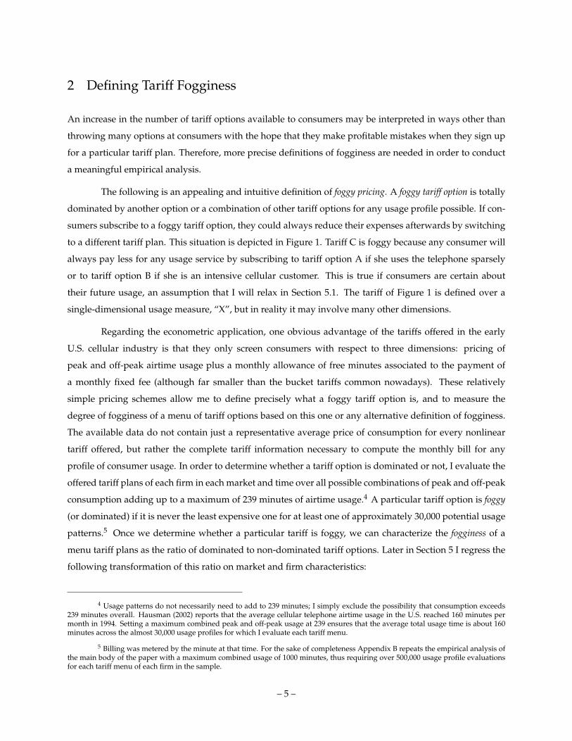
The following is an appealing and intuitive definition of foggy pricing. A foggy tariff option is totally

dominated by another option or a combination of other tariff options for any usage profile possible. If con-

sumers subscribe to a foggy tariff option, they could always reduce their expenses afterwards by switching

to a different tariff plan. This situation is depicted in Figure 1. Tariff C is foggy because any consumer will

always pay less for any usage service by subscribing to tariff option A if she uses the telephone sparsely

or to tariff option B if she is an intensive cellular customer. This is true if consumers are certain about

their future usage, an assumption that I will relax in Section 5.1. The tariff of Figure 1 is defined over a

single-dimensional usage measure, “X”, but in reality it may involve many other dimensions.

Regarding the econometric application, one obvious advantage of the tariffs offered in the early

U.S. cellular industry is that they only screen consumers with respect to three dimensions: pricing of

peak and off-peak airtime usage plus a monthly allowance of free minutes associated to the payment of

a monthly fixed fee (although far smaller than the bucket tariffs common nowadays). These relatively

simple pricing schemes allow me to define precisely what a foggy tariff option is, and to measure the

degree of fogginess of a menu of tariff options based on this one or any alternative definition of fogginess.

The available data do not contain just a representative average price of consumption for every nonlinear

tariff offered, but rather the complete tariff information necessary to compute the monthly bill for any

profile of consumer usage. In order to determine whether a tariff option is dominated or not, I evaluate the

offered tariff plans of each firm in each market and time over all possible combinations of peak and off-peak

consumption adding up to a maximum of 239 minutes of airtime usage.4 A particular tariff option is foggy

(or dominated) if it is never the least expensive one for at least one of approximately 30,000 potential usage

patterns.5 Once we determine whether a particular tariff is foggy, we can characterize the fogginess of a

menu tariff plans as the ratio of dominated to non-dominated tariff options. Later in Section 5 I regress the

following transformation of this ratio on market and firm characteristics:

4 Usage patterns do not necessarily need to add to 239 minutes; I simply exclude the possibility that consumption exceeds239 minutes overall. Hausman (2002) reports that the average cellular telephone airtime usage in the U.S. reached 160 minutes permonth in 1994. Setting a maximum combined peak and off-peak usage at 239 ensures that the average total usage time is about 160minutes across the almost 30,000 usage profiles for which I evaluate each tariff menu.

5 Billing was metered by the minute at that time. For the sake of completeness Appendix B repeats the empirical analysis ofthe main body of the paper with a maximum combined usage of 1000 minutes, thus requiring over 500,000 usage profile evaluationsfor each tariff menu of each firm in the sample.

– 5 –

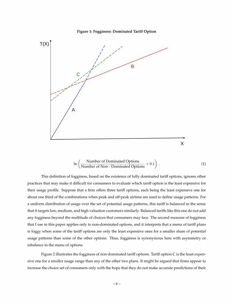
Figure 1: Fogginess: Dominated Tariff Option

X

T(X)

A

B

C

ln(

Number of Dominated OptionsNumber of Non−Dominated Options

+ 0.1)

. (1)

This definition of fogginess, based on the existence of fully dominated tariff options, ignores other

practices that may make it difficult for consumers to evaluate which tariff option is the least expensive for

their usage profile. Suppose that a firm offers three tariff options, each being the least expensive one for

about one third of the combinations when peak and off-peak airtime are used to define usage patterns. For

a uniform distribution of usage over the set of potential usage patterns, this tariff is balanced in the sense

that it targets low, medium, and high valuation customers similarly. Balanced tariffs like this one do not add

any fogginess beyond the multitude of choices that consumers may face. The second measure of fogginess

that I use in this paper applies only to non-dominated options, and it interprets that a menu of tariff plans

is foggy when some of the tariff options are only the least expensive ones for a smaller share of potential

usage patterns than some of the other options. Thus, fogginess is synonymous here with asymmetry or

inbalance in the menu of options.

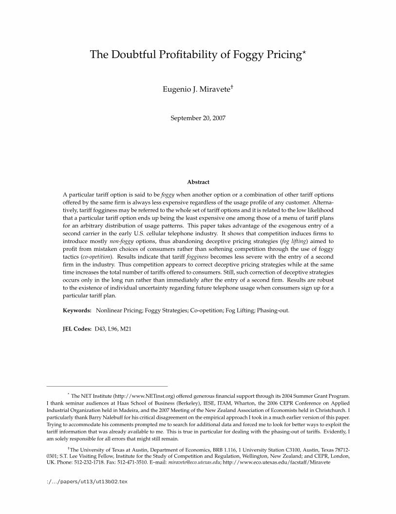
Figure 2 illustrates the fogginess of non-dominated tariff options. Tariff option C is the least expen-

sive one for a smaller usage range than any of the other two plans. It might be argued that firms appear to

increase the choice set of consumers only with the hope that they do not make accurate predictions of their

– 6 –

Figure 2: Fogginess: Non-Dominated Tariff Options

X

T(X)

A

B

C

future usage when subscribing to a particular tariff option.6 If a consumer chooses an option that is only the

least expensive one for a very limited usage range, she will most likely end up paying more for her realized

telephone usage (e.g., on the dashed portions of tariff option C in Figure 2) unless she is extremely accurate

in predicting her future usage. But for now, I simply ignore the potential effect of individual uncertainty

regarding future usage at the time of subscribing one particular tariff option.

The index of fogginess of non-dominated options thus needs to accommodate potential asymme-

tries regarding the share of usage patterns for which they are the least expensive option. There is little

doubt that a firm is engaging in foggy tactics when it gives consumers the choice among ten different tariff

options, none of which are strictly dominated, but some being the least expensive option for only three out

of the approximately 30,000 potential usage patterns (for which I evaluate every tariff option of each firm

in each market and time). The second proposed fogginess index characterizes this behavior as more foggy

than offering only two tariff plans that are the least expensive ones for approximately the same number

of usage patterns. To capture the effect of asymmetric menus of tariffs, I define the fogginess index of a

non-dominated set of tariff options as:

ϕ = n · HHI − 1 , (2)

6 An alternative and valid argument would justify offering tariff option C because of a certain concentration of consumptionpatterns around intermediate levels of usage. Since consumer types are not observable I implicitly assume that usage profiles areuniformly distributed and analyze whether a menu of tariff options is more or less balanced.

– 7 –

where n is the number of non-dominated tariff options offered and HHI is the Herfindahl-Hirschman index

of concentration defined over the share of usage patterns for which each plan is the least expensive one.

Considering only “balanced” tariff schedules in which each plan is the least expensive for the same 1/n

share of usage patterns, ϕ = 0 regardless of n, the number of tariff options offered. Because HHI increases

with the asymmetry of the distribution of shares of the least expensive usage patterns of each tariff option

—see Tirole (1989, §5.5)— the proposed index of fogginess also increases with a less balanced menus of

tariffs. Thus, Section 5 also regresses the following transformation of this Herfindahl-analog fogginess

measure on market and firm characteristics:

ln (ϕ + 0.1) . (3)

3 Pricing in the Early U.S. Cellular Industry

This paper studies the pricing strategies of numerous cellular telephone carriers in the early U.S. cellular

telephone industry. The data set is unique in the sense that it includes a fairly complete description of the

nonlinear tariff options offered by each firm over almost a decade. Most importantly, due to the institutional

developments surrounding the awarding of licenses, the data allows me to distinguish between monopoly

and duopoly regimes, the transition from the former to the latter depending on an exogenous judicial

decision in each market. Thus, this data set proves particularly useful to analyzing the effect of competition

on pricing behavior of firms and address, such as for instance, the issue of foggy pricing.

Some background information might be needed. By the mid 1980s, the Federal Communications

Commission (FCC) granted permission to create 305 non–overlapping cellular telephone markets around

metropolitan areas (SMSAs). Concerns about the viability of a fully competitive model led the FCC to

authorize only two carriers in each market. One of the two cellular licenses —the B block or wireline

license— was awarded to a local wireline carrier, i.e., a company with experience in fixed telephony, while

the A block —the nonwireline license— was initially awarded by comparative hearing to a carrier other than

the local wireline incumbent. Licenses were awarded in ten tiers, from more to less populated markets, be-

ginning in 1984. In general the wireline licensee offered the service first and enjoyed a temporary monopoly

position until the nonwireline carrier entered the market, normally within six months of being awarded

the license as required by the FCC. However, the administrative review process to award these licenses

among hundreds of contenders based only on technical issues and investment commitments proved to

be far more costly than initially expected. After awarding the first 30 SMSA licenses by means of this

expensive and time consuming beauty contest —there were up to 579 contenders for a single license— and

while the application review of the second tier of 30 markets was on its way, rules were adopted to award

the remaining nonwireline licenses through lotteries. Court appeals against the administrative award of

– 8 –

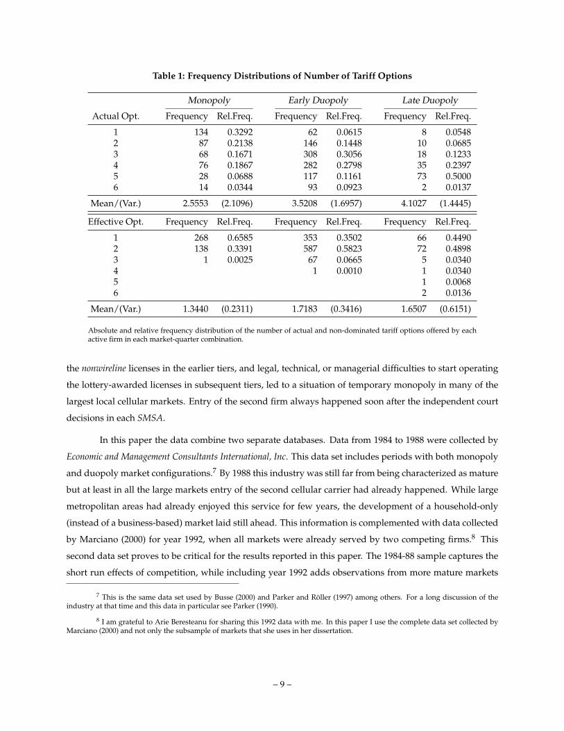
Table 1: Frequency Distributions of Number of Tariff Options

Monopoly Early Duopoly Late Duopoly

Actual Opt. Frequency Rel.Freq. Frequency Rel.Freq. Frequency Rel.Freq.

1 134 0.3292 62 0.0615 8 0.05482 87 0.2138 146 0.1448 10 0.06853 68 0.1671 308 0.3056 18 0.12334 76 0.1867 282 0.2798 35 0.23975 28 0.0688 117 0.1161 73 0.50006 14 0.0344 93 0.0923 2 0.0137

Mean/(Var.) 2.5553 (2.1096) 3.5208 (1.6957) 4.1027 (1.4445)

Effective Opt. Frequency Rel.Freq. Frequency Rel.Freq. Frequency Rel.Freq.

1 268 0.6585 353 0.3502 66 0.44902 138 0.3391 587 0.5823 72 0.48983 1 0.0025 67 0.0665 5 0.03404 1 0.0010 1 0.03405 1 0.00686 2 0.0136

Mean/(Var.) 1.3440 (0.2311) 1.7183 (0.3416) 1.6507 (0.6151)

Absolute and relative frequency distribution of the number of actual and non-dominated tariff options offered by eachactive firm in each market-quarter combination.

the nonwireline licenses in the earlier tiers, and legal, technical, or managerial difficulties to start operating

the lottery-awarded licenses in subsequent tiers, led to a situation of temporary monopoly in many of the

largest local cellular markets. Entry of the second firm always happened soon after the independent court

decisions in each SMSA.

In this paper the data combine two separate databases. Data from 1984 to 1988 were collected by

Economic and Management Consultants International, Inc. This data set includes periods with both monopoly

and duopoly market configurations.7 By 1988 this industry was still far from being characterized as mature

but at least in all the large markets entry of the second cellular carrier had already happened. While large

metropolitan areas had already enjoyed this service for few years, the development of a household-only

(instead of a business-based) market laid still ahead. This information is complemented with data collected

by Marciano (2000) for year 1992, when all markets were already served by two competing firms.8 This

second data set proves to be critical for the results reported in this paper. The 1984-88 sample captures the

short run effects of competition, while including year 1992 adds observations from more mature markets

7 This is the same data set used by Busse (2000) and Parker and Röller (1997) among others. For a long discussion of theindustry at that time and this data in particular see Parker (1990).

8 I am grateful to Arie Beresteanu for sharing this 1992 data with me. In this paper I use the complete data set collected byMarciano (2000) and not only the subsample of markets that she uses in her dissertation.

– 9 –

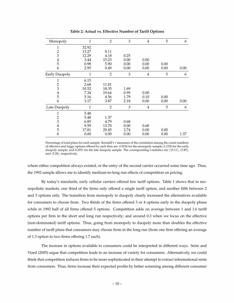
Table 2: Actual vs. Effective Number of Tariff Options

Monopoly 1 2 3 4 5 6

1 32.922 13.27 8.113 12.29 4.18 0.254 3.44 15.23 0.00 0.005 0.98 5.90 0.00 0.00 0.006 2.95 0.49 0.00 0.00 0.00 0.00

Early Duopoly 1 2 3 4 5 6

1 6.152 2.68 11.813 10.52 18.35 1.694 7.34 19.64 0.99 0.005 5.16 4.56 1.79 0.10 0.006 3.17 3.87 2.18 0.00 0.00 0.00

Late Duopoly 1 2 3 4 5 6

1 5.482 5.48 1.373 6.85 4.79 0.684 9.59 13.70 0.00 0.685 17.81 29.45 2.74 0.00 0.006 0.00 0.00 0.00 0.00 0.00 1.37

Percentage of total plans for each sample. Kendall’s τ measures of the correlation among the count numbersof effective and foggy options offered by each firm are: 0.5016 for the monopoly sample, 0.1230 for the earlyduopoly sample, and 0.2951 for the late duopoly sample. The corresponding t-statistics are (15.11), (5.85),and (5.28), respectively.

where either competition always existed, or the entry of the second carrier occurred some time ago. Thus,

the 1992 sample allows me to identify medium-to-long run effects of competition on pricing.

By today’s standards, early cellular carriers offered few tariff options. Table 1 shows that in mo-

nopolistic markets, one third of the firms only offered a single tariff option, and another fifth between 2

and 3 options only. The transition from monopoly to duopoly clearly increased the alternatives available

for consumers to choose from. Two thirds of the firms offered 3 or 4 options early in the duopoly phase

while in 1992 half of all firms offered 5 options. Competition adds on average between 1 and 1.6 tariff

options per firm in the short and long run respectively; and around 0.3 when we focus on the effective

(non-dominated) tariff options. Thus, going from monopoly to duopoly more than doubles the effective

number of tariff plans that consumers may choose from in the long run (from one firm offering an average

of 1.3 option to two firms offering 1.7 each).

The increase in options available to consumers could be interpreted in different ways. Seim and

Viard (2005) argue that competition leads to an increase of variety for consumers. Alternatively, we could

think that competition induces firms to be more sophisticated in their attempt to extract informational rents

from consumers. Thus, firms increase their expected profits by better screening among different consumer

– 10 –

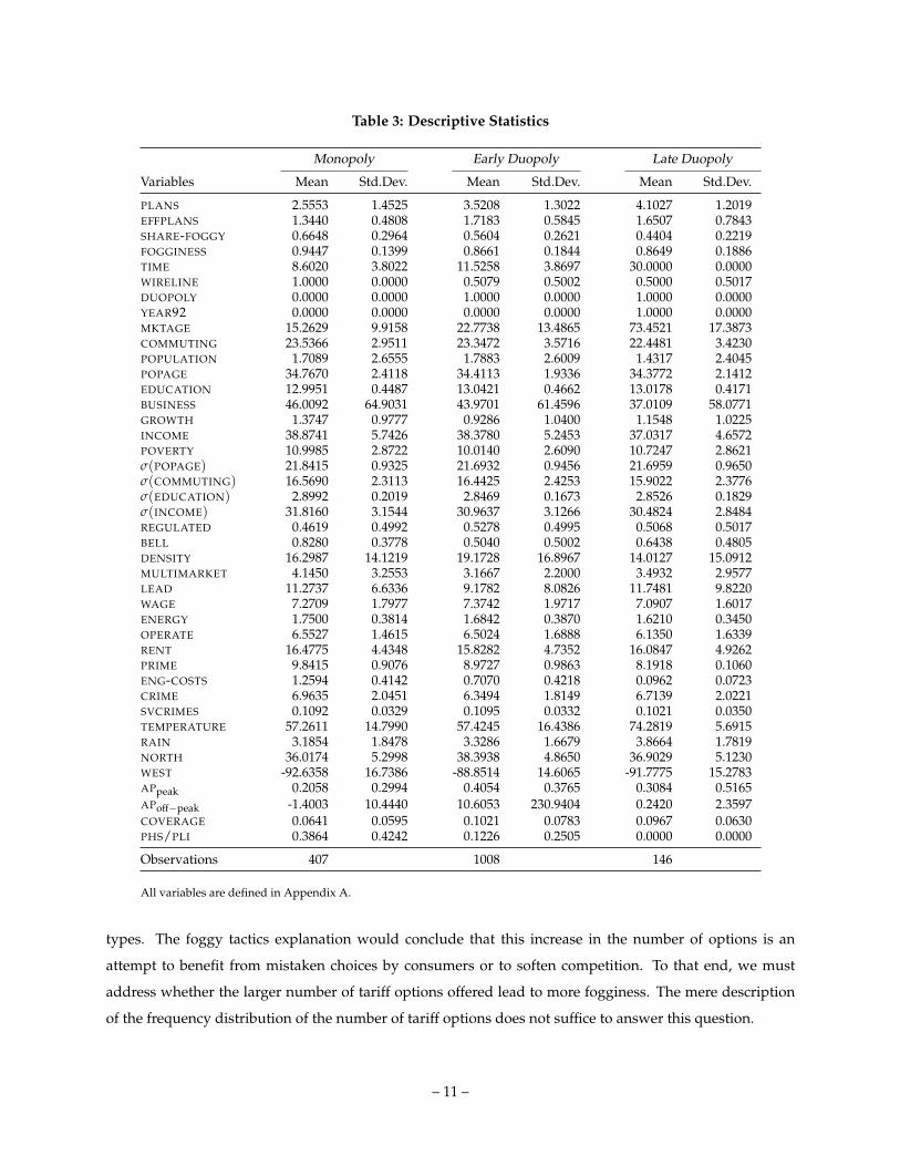
Table 3: Descriptive Statistics

Monopoly Early Duopoly Late Duopoly

Variables Mean Std.Dev. Mean Std.Dev. Mean Std.Dev.

PLANS 2.5553 1.4525 3.5208 1.3022 4.1027 1.2019EFFPLANS 1.3440 0.4808 1.7183 0.5845 1.6507 0.7843SHARE-FOGGY 0.6648 0.2964 0.5604 0.2621 0.4404 0.2219FOGGINESS 0.9447 0.1399 0.8661 0.1844 0.8649 0.1886TIME 8.6020 3.8022 11.5258 3.8697 30.0000 0.0000WIRELINE 1.0000 0.0000 0.5079 0.5002 0.5000 0.5017DUOPOLY 0.0000 0.0000 1.0000 0.0000 1.0000 0.0000YEAR92 0.0000 0.0000 0.0000 0.0000 1.0000 0.0000MKTAGE 15.2629 9.9158 22.7738 13.4865 73.4521 17.3873COMMUTING 23.5366 2.9511 23.3472 3.5716 22.4481 3.4230POPULATION 1.7089 2.6555 1.7883 2.6009 1.4317 2.4045POPAGE 34.7670 2.4118 34.4113 1.9336 34.3772 2.1412EDUCATION 12.9951 0.4487 13.0421 0.4662 13.0178 0.4171BUSINESS 46.0092 64.9031 43.9701 61.4596 37.0109 58.0771GROWTH 1.3747 0.9777 0.9286 1.0400 1.1548 1.0225INCOME 38.8741 5.7426 38.3780 5.2453 37.0317 4.6572POVERTY 10.9985 2.8722 10.0140 2.6090 10.7247 2.8621σ(POPAGE) 21.8415 0.9325 21.6932 0.9456 21.6959 0.9650σ(COMMUTING) 16.5690 2.3113 16.4425 2.4253 15.9022 2.3776σ(EDUCATION) 2.8992 0.2019 2.8469 0.1673 2.8526 0.1829σ(INCOME) 31.8160 3.1544 30.9637 3.1266 30.4824 2.8484REGULATED 0.4619 0.4992 0.5278 0.4995 0.5068 0.5017BELL 0.8280 0.3778 0.5040 0.5002 0.6438 0.4805DENSITY 16.2987 14.1219 19.1728 16.8967 14.0127 15.0912MULTIMARKET 4.1450 3.2553 3.1667 2.2000 3.4932 2.9577LEAD 11.2737 6.6336 9.1782 8.0826 11.7481 9.8220WAGE 7.2709 1.7977 7.3742 1.9717 7.0907 1.6017ENERGY 1.7500 0.3814 1.6842 0.3870 1.6210 0.3450OPERATE 6.5527 1.4615 6.5024 1.6888 6.1350 1.6339RENT 16.4775 4.4348 15.8282 4.7352 16.0847 4.9262PRIME 9.8415 0.9076 8.9727 0.9863 8.1918 0.1060ENG-COSTS 1.2594 0.4142 0.7070 0.4218 0.0962 0.0723CRIME 6.9635 2.0451 6.3494 1.8149 6.7139 2.0221SVCRIMES 0.1092 0.0329 0.1095 0.0332 0.1021 0.0350TEMPERATURE 57.2611 14.7990 57.4245 16.4386 74.2819 5.6915RAIN 3.1854 1.8478 3.3286 1.6679 3.8664 1.7819NORTH 36.0174 5.2998 38.3938 4.8650 36.9029 5.1230WEST -92.6358 16.7386 -88.8514 14.6065 -91.7775 15.2783APpeak 0.2058 0.2994 0.4054 0.3765 0.3084 0.5165APoff−peak -1.4003 10.4440 10.6053 230.9404 0.2420 2.3597COVERAGE 0.0641 0.0595 0.1021 0.0783 0.0967 0.0630PHS/PLI 0.3864 0.4242 0.1226 0.2505 0.0000 0.0000

Observations 407 1008 146

All variables are defined in Appendix A.

types. The foggy tactics explanation would conclude that this increase in the number of options is an

attempt to benefit from mistaken choices by consumers or to soften competition. To that end, we must

address whether the larger number of tariff options offered lead to more fogginess. The mere description

of the frequency distribution of the number of tariff options does not suffice to answer this question.

– 11 –

Tariffs in this early industry were quite simple. A tariff option was normally a two-part tariff with a

fixed monthly fee and a fixed rate per minute. Tariff options normally distinguish between peak (compris-

ing about 13 hours a day at that time) and off-peak marginal rates and sometimes included an allowance

of “free” minutes associated to the payment of the fixed monthly fee. Thus, the available combination

of monthly fee, marginal rates and usage allowance defines the tariff option completely and accurately.

Other value added services such as detailed billing, call waiting, no-answer transfer, call forwarding, three

way calling, busy transfer, call restriction, and voice mail were priced independently and rarely bundled

together with particular tariff options. This unique feature of the data allows me to analyze whether a

particular tariff option is dominated by one or a combination of some other available tariff options. Fur-

thermore, since the data (for the 1984-88 sample) were recorded every time that a firm changes its offering,

it is possible for me to trace the history of every tariff option and determine whether a dominated tariff

today is simply the result of phasing-out previously effective options.

The second half of Table 1 reports the frequency distribution of those tariff options that are non-

dominated. During the monopoly phase firms offered on average 1.2 dominated options, a number that

climbs to 1.8 right after the entry of the second carrier and to 2.5 in the long run. Evidently not all firms

made use of foggy pricing with the same intensity. While the average number of foggy plans increases with

competition according to Table 1, Table 2 shows that the number of tariff foggy options vary substantially

with the total number of tariff options offered. For instance, during the monopoly phase firms offered

one foggy option out of two alternatives in 13.27% of cases. With competition this percentage dropped

immediately to 2.68% although later increased to 5.48%. On the contrary, situations when one out of five

options were foggy went up from 0.98% to 5.16% in the short run and 17.81% of cases in the long run.

Therefore, there are movements in the opposite direction. Easy to detect cases with a foggy option out of a

few become less common while more difficult cases to detect with one foggy option out of many become

less rare. Thus, the effect of competition on the fogginess of tariffs offered is, at this stage, ambiguous. To

determine the effect of competition, I conduct a simple econometric analysis in which I control for many

observable market and firm specific characteristics. Hence, tariff data are complemented with market

specific demand and cost information for each firm. Descriptive statistics are reported in Table 3 and

definition of variables are included in Appendix A.

4 Actual and Effective Number of Tariff Options

In many industries consumer heterogeneity is important. If arbitrage can be easily avoided firms can

increase their expected profits by offering a nonlinear tariff that optimally discriminates among consumers

with different levels of willingness to pay. Optimal nonlinear pricing leads to offering discounts to larger

consumers, who in turn face marginal charges closer to marginal costs. Thus, the optimal tariff is an

– 12 –

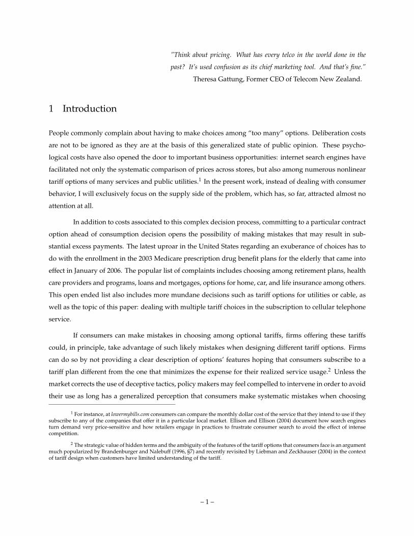
increasing and concave function under very general conditions, and the degree of concavity is intimately

linked to the spread of the distribution of consumer types. This result is formally proven by Maskin and

Riley (1984) and Wilson (1993). Figure 3 illustrates this point.

Oi (1971) observes that if all consumers are alike a simple two-part tariff such as “Schedule A” of

Figure 3 suffices to extract all consumer surplus and achieves the first best solution: the marginal charge

should equal marginal cost c and the fixed fee amounts to the size of the associated consumer surplus.

If consumers are heterogeneous, a different unit price has to be offered to each consumer type in order to

extract as much surplus as possible while avoiding arbitrage. As the proportion of high valuation customers

increases among the population of active consumers, firms need to charge higher markups for low usage

customers in order for the tariff to qualify as an incentive compatible contract that avoids high valuation

customers mimicking the behavior of low valuation ones. Thus, “Schedule B” is the optimal tariff when

some high valuation consumers are present and “Schedule C” is optimal when the population includes

many more high than low valuation customers.9 I include APpeak and APoff−peak as regressors to account

for the degree of concavity of the lower envelope of the different tariff options offered. Variable APpeak is the

equivalent of the Arrow-Pratt measure of risk aversion averaged over the 0-239 minute interval of airtime

usage of the quadratic polynomial that fits the lower envelope of the peak component of the tariff. Variable

APoff−peak is defined similarly but using the off-peak component of the tariff only.10

Column A1 of Table 4 presents the results of estimating a Poisson pseudo maximum likelihood estima-

tion (PMLE) count data model that relates the observed market and firm characteristics to the number of

tariff options offered by each firm according to the following exponential mean function:

E [PLANS | X] = exp(X ′β

). (4)

Similarly, column B1 of Table 4 focuses on the number of effective tariff options only, i.e., those who are the

least expensive ones for at least few consumption profiles.11 The other two columns, A2 and B2 are PMLE

estimates that control for the potential endogeneity of APpeak, APoff−peak, and COVERAGE. Since firms can

make use of available market characteristics to control for the nature of the distribution of consumers’

9 The connection between the degree of concavity of the optimal tariff and the statistical properties of the distribution ofconsumer types is analyzed extensively by Miravete (2005).

10 This approach is equivalent to the discrete Arrow-Pratt measure employed by Marciano (2000, §4.2) to account for thecurvature of the tariff. Similar results were obtained with the Cobb-Douglas approximation to the lower envelope of the tariff of Busseand Rysman (2005).

11 The variance of a Poisson distribution is identical to the mean. Thus, inference can be seriously compromised if the expecteddistributions of PLANS and EFFPLANS conditional on X are not equidispersed. The PMLE estimation method obtains consistentestimates of β based on the Poisson likelihood function, but employs a robust covariance matrix that allows for both overdispersionand the less common underdispersion, which happens to be what characterizes the empirical distribution of both total and effectivenumber of plans in the present sample according to Table 1. The advantages of the robust PMLE estimation and the computation ofthe robust covariance matrix is discussed at length by Cameron and Trivedi (1998, §3.2.3), Gourieroux, Monfort, and Trognon (1984),and Wooldridge (2002, 19.2.2).

– 13 –

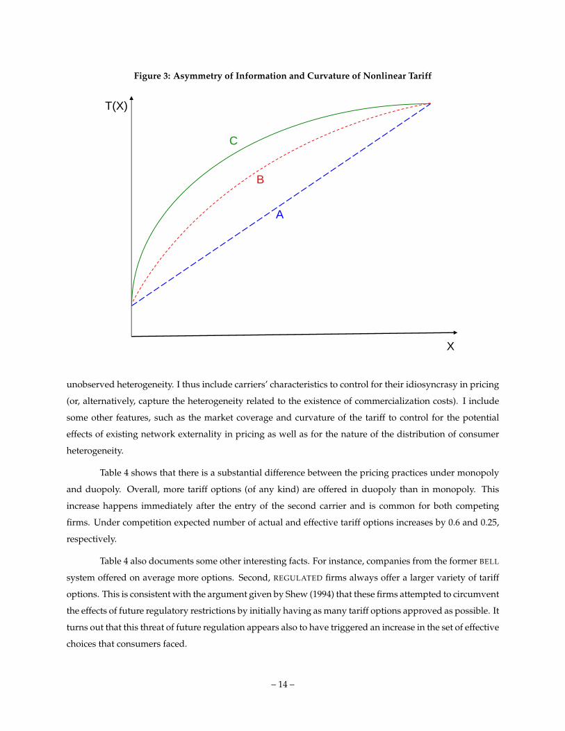
Figure 3: Asymmetry of Information and Curvature of Nonlinear Tariff

X

T(X)

A

B

C

unobserved heterogeneity. I thus include carriers’ characteristics to control for their idiosyncrasy in pricing

(or, alternatively, capture the heterogeneity related to the existence of commercialization costs). I include

some other features, such as the market coverage and curvature of the tariff to control for the potential

effects of existing network externality in pricing as well as for the nature of the distribution of consumer

heterogeneity.

Table 4 shows that there is a substantial difference between the pricing practices under monopoly

and duopoly. Overall, more tariff options (of any kind) are offered in duopoly than in monopoly. This

increase happens immediately after the entry of the second carrier and is common for both competing

firms. Under competition expected number of actual and effective tariff options increases by 0.6 and 0.25,

respectively.

Table 4 also documents some other interesting facts. For instance, companies from the former BELL

system offered on average more options. Second, REGULATED firms always offer a larger variety of tariff

options. This is consistent with the argument given by Shew (1994) that these firms attempted to circumvent

the effects of future regulatory restrictions by initially having as many tariff options approved as possible. It

turns out that this threat of future regulation appears also to have triggered an increase in the set of effective

choices that consumers faced.

– 14 –

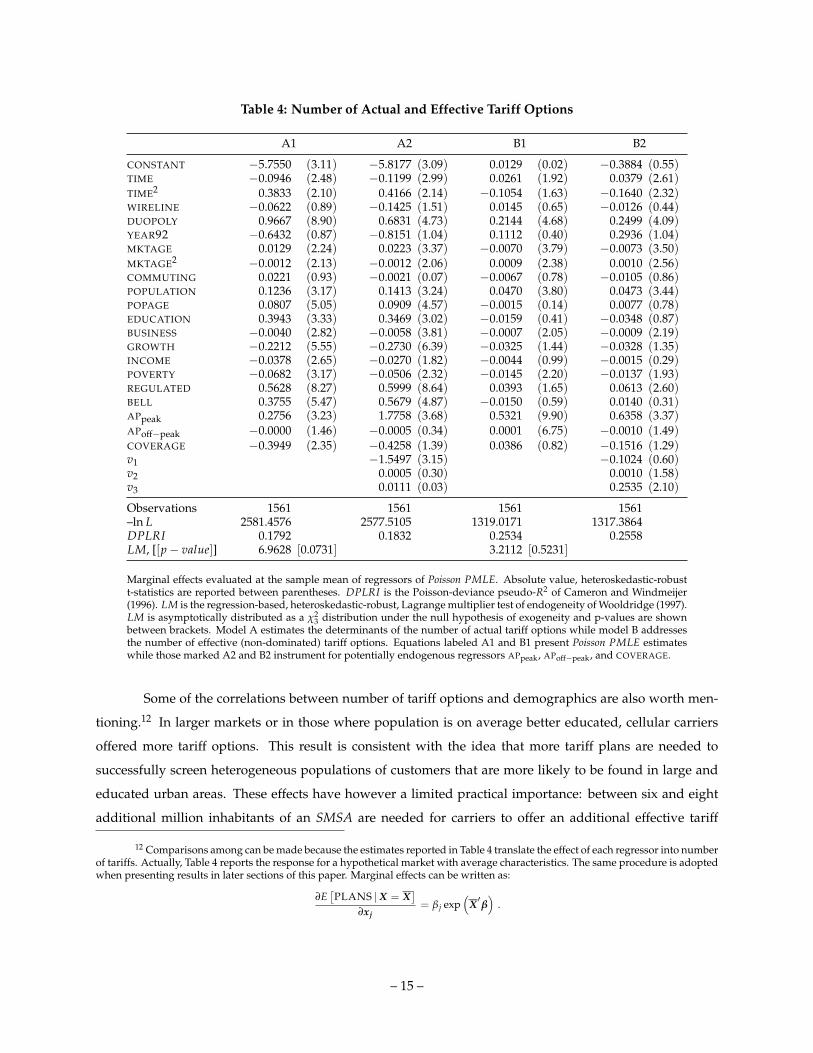
Table 4: Number of Actual and Effective Tariff Options

A1 A2 B1 B2

CONSTANT −5.7550 (3.11) −5.8177 (3.09) 0.0129 (0.02) −0.3884 (0.55)TIME −0.0946 (2.48) −0.1199 (2.99) 0.0261 (1.92) 0.0379 (2.61)TIME2 0.3833 (2.10) 0.4166 (2.14) −0.1054 (1.63) −0.1640 (2.32)WIRELINE −0.0622 (0.89) −0.1425 (1.51) 0.0145 (0.65) −0.0126 (0.44)DUOPOLY 0.9667 (8.90) 0.6831 (4.73) 0.2144 (4.68) 0.2499 (4.09)YEAR92 −0.6432 (0.87) −0.8151 (1.04) 0.1112 (0.40) 0.2936 (1.04)MKTAGE 0.0129 (2.24) 0.0223 (3.37) −0.0070 (3.79) −0.0073 (3.50)MKTAGE2 −0.0012 (2.13) −0.0012 (2.06) 0.0009 (2.38) 0.0010 (2.56)COMMUTING 0.0221 (0.93) −0.0021 (0.07) −0.0067 (0.78) −0.0105 (0.86)POPULATION 0.1236 (3.17) 0.1413 (3.24) 0.0470 (3.80) 0.0473 (3.44)POPAGE 0.0807 (5.05) 0.0909 (4.57) −0.0015 (0.14) 0.0077 (0.78)EDUCATION 0.3943 (3.33) 0.3469 (3.02) −0.0159 (0.41) −0.0348 (0.87)BUSINESS −0.0040 (2.82) −0.0058 (3.81) −0.0007 (2.05) −0.0009 (2.19)GROWTH −0.2212 (5.55) −0.2730 (6.39) −0.0325 (1.44) −0.0328 (1.35)INCOME −0.0378 (2.65) −0.0270 (1.82) −0.0044 (0.99) −0.0015 (0.29)POVERTY −0.0682 (3.17) −0.0506 (2.32) −0.0145 (2.20) −0.0137 (1.93)REGULATED 0.5628 (8.27) 0.5999 (8.64) 0.0393 (1.65) 0.0613 (2.60)BELL 0.3755 (5.47) 0.5679 (4.87) −0.0150 (0.59) 0.0140 (0.31)APpeak 0.2756 (3.23) 1.7758 (3.68) 0.5321 (9.90) 0.6358 (3.37)APoff−peak −0.0000 (1.46) −0.0005 (0.34) 0.0001 (6.75) −0.0010 (1.49)COVERAGE −0.3949 (2.35) −0.4258 (1.39) 0.0386 (0.82) −0.1516 (1.29)v1 −1.5497 (3.15) −0.1024 (0.60)v2 0.0005 (0.30) 0.0010 (1.58)v3 0.0111 (0.03) 0.2535 (2.10)

Observations 1561 1561 1561 1561–ln L 2581.4576 2577.5105 1319.0171 1317.3864DPLRI 0.1792 0.1832 0.2534 0.2558LM, [[p − value]] 6.9628 [0.0731] 3.2112 [0.5231]

Marginal effects evaluated at the sample mean of regressors of Poisson PMLE. Absolute value, heteroskedastic-robustt-statistics are reported between parentheses. DPLRI is the Poisson-deviance pseudo-R2 of Cameron and Windmeijer(1996). LM is the regression-based, heteroskedastic-robust, Lagrange multiplier test of endogeneity of Wooldridge (1997).LM is asymptotically distributed as a χ2

3 distribution under the null hypothesis of exogeneity and p-values are shownbetween brackets. Model A estimates the determinants of the number of actual tariff options while model B addressesthe number of effective (non-dominated) tariff options. Equations labeled A1 and B1 present Poisson PMLE estimateswhile those marked A2 and B2 instrument for potentially endogenous regressors APpeak, APoff−peak, and COVERAGE.

Some of the correlations between number of tariff options and demographics are also worth men-

tioning.12 In larger markets or in those where population is on average better educated, cellular carriers

offered more tariff options. This result is consistent with the idea that more tariff plans are needed to

successfully screen heterogeneous populations of customers that are more likely to be found in large and

educated urban areas. These effects have however a limited practical importance: between six and eight

additional million inhabitants of an SMSA are needed for carriers to offer an additional effective tariff

12 Comparisons among can be made because the estimates reported in Table 4 translate the effect of each regressor into numberof tariffs. Actually, Table 4 reports the response for a hypothetical market with average characteristics. The same procedure is adoptedwhen presenting results in later sections of this paper. Marginal effects can be written as:

∂E[PLANS | X = X

]∂xj

= β j exp(

X ′β)

.

– 15 –

option while EDUCATION stops being significant at all when we focus on effective rather than on actual tar-

iffs. Surprisingly, BUSINESS, and INCOME are negatively correlated with the number of actual and effective

tariff plans offered, although their negative effect is far smaller than the positive effect of POPULATION and

EDUCATION.

The last three regressors may all suffer from endogeneity. In the case of APpeak and APoff−peak, en-

dogeneity may arise because firms do not only decide on the number of tariff options, but also which tariff

options to offer, thus determining the curvature and position of the tariff lower envelope. Alternatively, we

could adopt the view that the distribution of consumer heterogeneity is exogenous and firms are simply

responding to this heterogeneity when they design the nonlinear tariff. Network externalities are another

potential source of endogeneity, as the demand for telephone services may depend on the number of total

subscribers in a market. Since pricing determines the decision to subscribe, the strategy followed by each

carrier is partly responsible for the net externality that a new customer may enjoy.13 Cellular telephones

were far less popular than they are today. By the end of our sample, there were only 11 million subscribers

(as compared to the current 208 million according to the CTIA’s November 2005 Semi-Annual Data Survey).

Therefore, the definition of COVERAGE used here accounts not only for residential, but also for potential

business customers.14

The second and fourth columns of Table 4 repeat the analysis of columns A and B after correcting for

endogeneity by the robust PMLE method of Wooldridge (1997), which consists of including the prediction

errors of the instrumental regressions of APpeak, APoff−peak, and COVERAGE on the Poisson PMLE count

data regression. The LM tests reported in Table 4 indicate that APpeak, APoff−peak, and COVERAGE can be

considered jointly exogenous although individually, APpeak appears to be endogenous in the equation of

the number of options and COVERAGE in the equation of the number of effective options. After correcting

for any endogeneity bias, the sign of estimates and conclusions of this section still stand.

5 Analysis of Fogginess

The observed increase of options available in competitive markets does not suffice to conclude that firms are

engaging in foggy pricing to take advantage of consumers’ deliberation costs. The mere increase of tariff op-

tions may be simply aimed to better screening heterogeneous consumers that are heterogeneous, something

that is supported by the fact that APpeak is exogenous in the equation of the number of effective tariff op-

13 This argument is admittedly weak for the early U.S. cellular telephone industry, since the service clearly aimed businessesand high income individuals. However, targeting a small group of customers could indeed lead to network externalities throughimitation of other members in a small social network.

14 This variable is approximated as 1,300 maximum customers per antenna site already built, divided by the sum of thenumber of business considered as high potential customers and the number of (assumed four member) families in each SMSA. For adetailed discussion on this definition see Basaluzzo and Miravete (2007, §2).

– 16 –

tions. Complexity of telecommunications tariffs is related not only to the number of tariff options offered by

telephone carriers, but to the different dimensions of pricing considered such as peak/shoulder/off-peak,

distance, identity of the called party, network terminating the call, roaming charges, rollover minutes of

unused allowance, et cetera. This section studies whether fogginess of tariffs increases or decreases after the

entry of a second carrier in the cellular industry and aims to determine whether such a process is common

to all markets rather than specific to a few of them.

Table 5 reports the marginal effects of the two measures of fogginess proposed in Section 2. Results

assume that consumers do not face any uncertainty regarding future telephone usage when they subscribe

to a particular tariff plan. Potentially endogenous variables can be consider jointly exogenous and estimates

obtained after instrumenting these variables are of the same sign and size.

The Herfindahl-analog measure of fogginess related to non-dominated options does not show any

particular change over time and with the transition to a competitive regime. Deception certainly does not

increase as measured by equation 3 although it appears that wireline entrants are keener than nonwireline

incumbents in using tariff options that are the least expensive ones for a very small range of usage profiles.

But the effect is small and is one of the few that does not survive correcting for endogeneity.

More informative is the use of the ratio of dominated to non-dominated options to capture the

effect of competition on the use of deceptive strategies. Consistent with the results reported in Table 4,

right after the entry of the second cellular carrier, this ratio increases indicating that foggy tactics become

more common with competition than in a monopoly. However, this is result does not fully describes the

effect of competition on the use of foggy pricing. This is just the short run effect. The long run effect

captured by YEAR92 is negative and significantly larger (in absolute value), indicating that the use of foggy

pricing is not sustainable in the long run and that competition in the end reduces the proportion of contract

options offered to consumers aimed solely to benefit from their mistakes.

In addition, Table 5 documents that, the reduction in fogginess is uneven across markets and results

critically depend on the measure of fogginess used. The ratio of dominated to non-dominated options

increases with MKTAGE, POPAGE, EDUCATION, if the market is REGULATED, or if the carrier used to be part

of the BELL system. On the contrary customers living in markets with a large number of BUSINESS a fast

GROWTH rate, or high INCOME enjoy less foggy pricing tactics. The behavior of the fogginess index for

non-dominated tariff options ϕ is similar although many of these regressors are not significant.

When consumers are very similar the optimal nonlinear tariff becomes most likely a simple two-

part tariff (as discussed in Figure 3). Thus, the Arrow-Pratt measure of degree of concavity approaches

zero. In general, it is in those cases when firms offer more foggy options. Firms make use of more complex

and deceptive strategies when adding another effective tariff option to further segment the market leads to

a very low increase in expected profits. However, this result, consistent with the argument put forward in

– 17 –

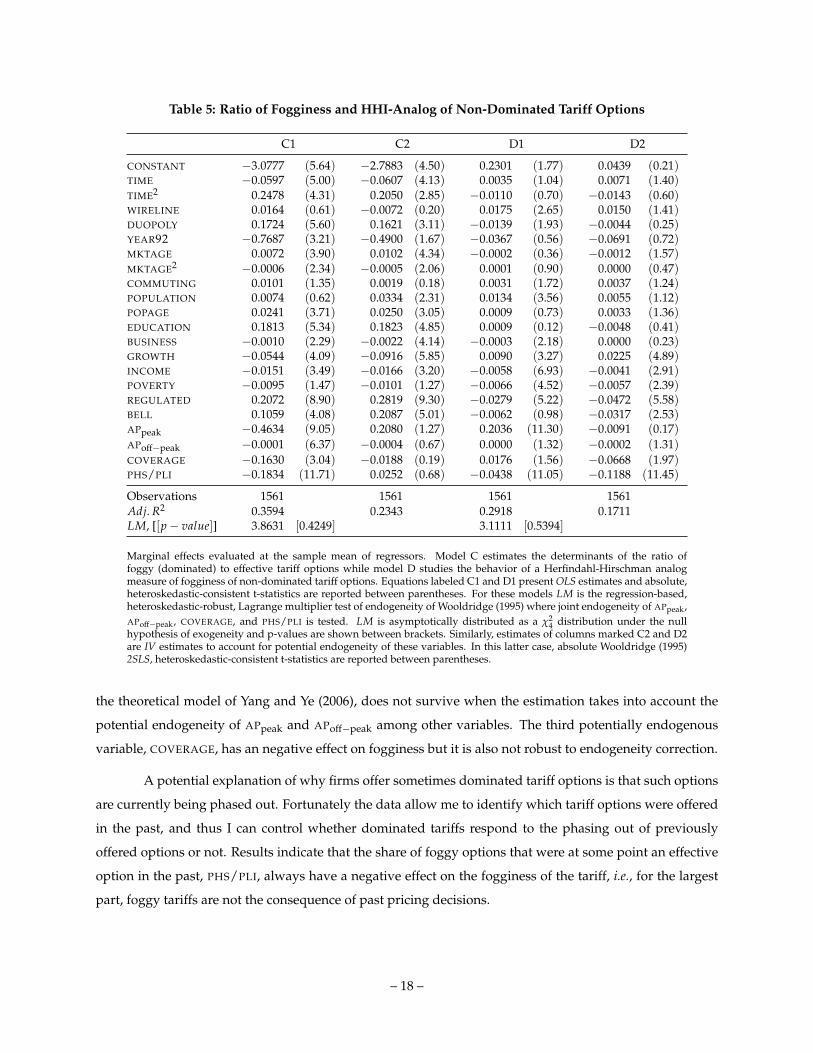
Table 5: Ratio of Fogginess and HHI-Analog of Non-Dominated Tariff Options

C1 C2 D1 D2

CONSTANT −3.0777 (5.64) −2.7883 (4.50) 0.2301 (1.77) 0.0439 (0.21)TIME −0.0597 (5.00) −0.0607 (4.13) 0.0035 (1.04) 0.0071 (1.40)TIME2 0.2478 (4.31) 0.2050 (2.85) −0.0110 (0.70) −0.0143 (0.60)WIRELINE 0.0164 (0.61) −0.0072 (0.20) 0.0175 (2.65) 0.0150 (1.41)DUOPOLY 0.1724 (5.60) 0.1621 (3.11) −0.0139 (1.93) −0.0044 (0.25)YEAR92 −0.7687 (3.21) −0.4900 (1.67) −0.0367 (0.56) −0.0691 (0.72)MKTAGE 0.0072 (3.90) 0.0102 (4.34) −0.0002 (0.36) −0.0012 (1.57)MKTAGE2 −0.0006 (2.34) −0.0005 (2.06) 0.0001 (0.90) 0.0000 (0.47)COMMUTING 0.0101 (1.35) 0.0019 (0.18) 0.0031 (1.72) 0.0037 (1.24)POPULATION 0.0074 (0.62) 0.0334 (2.31) 0.0134 (3.56) 0.0055 (1.12)POPAGE 0.0241 (3.71) 0.0250 (3.05) 0.0009 (0.73) 0.0033 (1.36)EDUCATION 0.1813 (5.34) 0.1823 (4.85) 0.0009 (0.12) −0.0048 (0.41)BUSINESS −0.0010 (2.29) −0.0022 (4.14) −0.0003 (2.18) 0.0000 (0.23)GROWTH −0.0544 (4.09) −0.0916 (5.85) 0.0090 (3.27) 0.0225 (4.89)INCOME −0.0151 (3.49) −0.0166 (3.20) −0.0058 (6.93) −0.0041 (2.91)POVERTY −0.0095 (1.47) −0.0101 (1.27) −0.0066 (4.52) −0.0057 (2.39)REGULATED 0.2072 (8.90) 0.2819 (9.30) −0.0279 (5.22) −0.0472 (5.58)BELL 0.1059 (4.08) 0.2087 (5.01) −0.0062 (0.98) −0.0317 (2.53)APpeak −0.4634 (9.05) 0.2080 (1.27) 0.2036 (11.30) −0.0091 (0.17)APoff−peak −0.0001 (6.37) −0.0004 (0.67) 0.0000 (1.32) −0.0002 (1.31)COVERAGE −0.1630 (3.04) −0.0188 (0.19) 0.0176 (1.56) −0.0668 (1.97)PHS/PLI −0.1834 (11.71) 0.0252 (0.68) −0.0438 (11.05) −0.1188 (11.45)

Observations 1561 1561 1561 1561Adj. R2 0.3594 0.2343 0.2918 0.1711LM, [[p − value]] 3.8631 [0.4249] 3.1111 [0.5394]

Marginal effects evaluated at the sample mean of regressors. Model C estimates the determinants of the ratio offoggy (dominated) to effective tariff options while model D studies the behavior of a Herfindahl-Hirschman analogmeasure of fogginess of non-dominated tariff options. Equations labeled C1 and D1 present OLS estimates and absolute,heteroskedastic-consistent t-statistics are reported between parentheses. For these models LM is the regression-based,heteroskedastic-robust, Lagrange multiplier test of endogeneity of Wooldridge (1995) where joint endogeneity of APpeak,APoff−peak, COVERAGE, and PHS/PLI is tested. LM is asymptotically distributed as a χ2

4 distribution under the nullhypothesis of exogeneity and p-values are shown between brackets. Similarly, estimates of columns marked C2 and D2are IV estimates to account for potential endogeneity of these variables. In this latter case, absolute Wooldridge (1995)2SLS, heteroskedastic-consistent t-statistics are reported between parentheses.

the theoretical model of Yang and Ye (2006), does not survive when the estimation takes into account the

potential endogeneity of APpeak and APoff−peak among other variables. The third potentially endogenous

variable, COVERAGE, has an negative effect on fogginess but it is also not robust to endogeneity correction.

A potential explanation of why firms offer sometimes dominated tariff options is that such options

are currently being phased out. Fortunately the data allow me to identify which tariff options were offered

in the past, and thus I can control whether dominated tariffs respond to the phasing out of previously

offered options or not. Results indicate that the share of foggy options that were at some point an effective

option in the past, PHS/PLI, always have a negative effect on the fogginess of the tariff, i.e., for the largest

part, foggy tariffs are not the consequence of past pricing decisions.

– 18 –

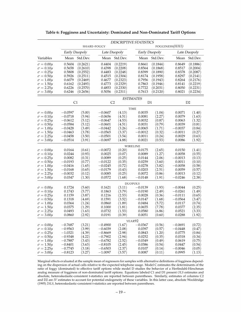
Table 6: Fogginess and Uncertainty: Dominated and Non-Dominated Tariff Options

DESCRIPTIVE STATISTICSSHARE-FOGGY FOGGINESS(HHI)

Early Duopoly Late Duopoly Early Duopoly Late Duopoly

Variables Mean Std.Dev. Mean Std.Dev. Mean Std.Dev. Mean Std.Dev.

σ = 0.00µ 0.5604 (0.2621) 0.4404 (0.2219) 0.8661 (0.1844) 0.8649 (0.1886)σ = 0.10µ 0.5658 (0.2610) 0.4398 (0.2208) 0.8564 (0.1868) 0.8517 (0.2004)σ = 0.25µ 0.5808 (0.2552) 0.4483 (0.2248) 0.8399 (0.1890) 0.8378 (0.2087)σ = 0.50µ 0.5926 (0.2511) 0.4515 (0.2304) 0.8174 (0.1958) 0.8297 (0.2141)σ = 1.00µ 0.6079 (0.2469) 0.4677 (0.2323) 0.7956 (0.1943) 0.8264 (0.2176)σ = 1.50µ 0.6162 (0.2493) 0.4773 (0.2329) 0.7863 (0.1946) 0.8141 (0.2219)σ = 2.25µ 0.6226 (0.2570) 0.4853 (0.2330) 0.7722 (0.2031) 0.8050 (0.2231)σ = 3.00µ 0.6246 (0.2656) 0.5056 (0.2311) 0.7613 (0.2120) 0.8021 (0.2234)

ESTIMATESC1 C2 D1 D2

TIMEσ = 0.00µ −0.0597 (5.00) −0.0607 (4.13) 0.0035 (1.04) 0.0071 (1.40)σ = 0.10µ −0.0718 (5.94) −0.0656 (4.51) 0.0081 (2.27) 0.0079 (1.63)σ = 0.25µ −0.0612 (5.12) −0.0647 (4.53) 0.0032 (0.87) 0.0063 (1.32)σ = 0.50µ −0.0584 (5.12) −0.0601 (4.51) 0.0031 (0.79) 0.0039 (0.81)σ = 1.00µ −0.0428 (3.49) −0.0442 (3.26) −0.0065 (1.71) −0.0037 (0.84)σ = 1.50µ −0.0463 (3.78) −0.0565 (3.37) −0.0012 (0.32) −0.0011 (0.27)σ = 2.25µ −0.0458 (3.50) −0.0501 (3.54) 0.0011 (0.24) 0.0029 (0.63)σ = 3.00µ −0.0514 (3.91) −0.0697 (4.88) 0.0021 (0.53) 0.0086 (1.92)

WIRELINEσ = 0.00µ 0.0164 (0.61) −0.0072 (0.20) 0.0175 (2.65) 0.0150 (1.41)σ = 0.10µ 0.0244 (0.93) 0.0025 (0.07) 0.0089 (1.27) 0.0058 (0.55)σ = 0.25µ 0.0082 (0.31) 0.0089 (0.25) 0.0144 (2.06) −0.0013 (0.13)σ = 0.50µ −0.0193 (0.77) −0.0122 (0.35) 0.0259 (3.60) 0.0011 (0.10)σ = 1.00µ −0.0416 (1.65) −0.0245 (0.72) 0.0278 (3.82) −0.0058 (0.58)σ = 1.50µ −0.0168 (0.65) −0.0179 (0.43) 0.0203 (2.51) 0.0059 (0.57)σ = 2.25µ −0.0032 (0.12) 0.0085 (0.25) 0.0072 (0.86) 0.0013 (0.12)σ = 3.00µ 0.0347 (1.30) 0.0572 (1.68) −0.0148 (1.91) −0.0246 (2.38)

DUOPOLYσ = 0.00µ 0.1724 (5.60) 0.1621 (3.11) −0.0139 (1.93) −0.0044 (0.25)σ = 0.10µ 0.1743 (5.77) 0.1863 (3.79) −0.0190 (2.49) −0.0261 (1.49)σ = 0.25µ 0.1159 (3.87) 0.1216 (2.53) 0.0028 (0.36) −0.0111 (0.65)σ = 0.50µ 0.1318 (4.69) 0.1591 (3.52) −0.0147 (1.68) −0.0564 (3.47)σ = 1.00µ 0.0364 (1.24) 0.0860 (1.89) 0.0484 (5.72) 0.0117 (0.74)σ = 1.50µ 0.0375 (1.29) 0.1000 (1.81) 0.0655 (7.78) 0.0377 (2.35)σ = 2.25µ 0.0493 (1.63) 0.0732 (1.53) 0.0580 (6.86) 0.0521 (3.33)σ = 3.00µ 0.0860 (2.92) 0.0191 (0.39) 0.0051 (0.60) 0.0288 (1.92)

YEAR92σ = 0.00µ −0.7687 (3.21) −0.4900 (1.67) −0.0367 (0.56) −0.0691 (0.72)σ = 0.10µ −0.9563 (3.99) −0.6039 (2.08) 0.0397 (0.57) −0.0448 (0.47)σ = 0.25µ −1.0321 (4.39) −0.8669 (2.98) 0.0843 (1.20) 0.0775 (0.84)σ = 0.50µ −0.9348 (4.22) −0.7902 (2.94) 0.0252 (0.35) 0.0318 (0.34)σ = 1.00µ −0.7887 (3.43) −0.6782 (2.52) −0.0349 (0.49) 0.0619 (0.75)σ = 1.50µ −0.8401 (3.63) −0.8105 (2.45) 0.0386 (0.54) 0.0447 (0.54)σ = 2.25µ −0.7745 (3.18) −0.6503 (2.37) 0.0107 (0.14) −0.0046 (0.05)σ = 3.00µ −0.8123 (3.27) −1.0097 (3.57) 0.0087 (0.11) 0.0995 (1.13)

Marginal effects evaluated at the sample mean of regressors for samples with alternative definitions of fogginess depend-ing on the dispersion of actual calls relative to the expected telephone usage. Model C estimates the determinants of theratio of foggy (dominated) to effective tariff options while model D studies the behavior of a Herfindahl-Hirschmananalog measure of fogginess of non-dominated tariff options. Equations labeled C1 and D1 present OLS estimates andabsolute, heteroskedastic-consistent t-statistics are reported between parentheses. Similarly, estimates of columns C2and D2 are IV estimates to account for potential endogeneity of these variables. In this latter case, absolute Wooldridge(1995) 2SLS, heteroskedastic-consistent t-statistics are reported between parentheses.

– 19 –

5.1 Robustness of Results to Consumers’ Uncertainty

Evidently consumers do not choose tariff options and telephone usage simultaneously. Indeed, consumers

first choose a tariff option and later decide how much to talk on the phone. Choosing a particular tariff

option does not force consumers to commit to any particular level of usage. Thus, the more accurate their

predictions are, the more valid are the results of Table 5.

In the absence of individual data I evaluate the robustness of the results reported above with respect

to the existence of individual uncertainty by means of simulations. For the analysis in Table 5 I first deter-

mined which tariff option was the least expensive for each potential usage profiles defined by almost 30,000

combinations (i, j) where i = 0, 1, 2, . . . represented the number of peak minutes a household uses during a

month and j = 0, 1, 2, . . . were the corresponding off-peak minutes of usage. Furthermore, it was assumed

that i + j ≤ 239 so that the average usage profile is 160 minutes a month, a magnitude that is representative

of the monthly usage during this early market. Now, in order to capture the existence of future usage

uncertainty among consumers, I identify which option leads to the lowest expected tariff payment when

the realized consumption profile can be understood as a random draw from a particular bivariate normal

distribution centered around (µi, µj), and s.t. µi + µj ≤ 239. Thus, µi and µj represent the expected number

peak and off-peak number of calls, respectively, that a household makes in a month. Usage in these two

dimensions are assumed to be independently distributed according to univariate normal distributions with

standard deviations proportional to the mean, i.e., σi = κµi and σj = κµj. This heteroskedastic assumption

captures the documented dispersion of telephone usage for different usage levels (e.g., Miravete (2005, §4)).

Therefore, for each of the approximately 30,000 expected usage profiles defined by (µi, µj) I compute the

expected payment under each tariff option by integrating out according to the assumed distributions of

usage. In particular I compute the average payment of a particular tariff option over fifty random draws

from N[µi, (κµi)2] for peak usage and another fifty from N[µj, (κµj)2] for off-peak usage. The process is

repeated for each of the 30,000 potential usage profiles as well as for increasing dispersions of usage as

measured by κ.

The top of Table 6 reports the descriptive statistics of the share of dominated tariff as well as the

Herfindahl-analog measure ϕ of fogginess of non-dominated tariffs under increasingly more dispersed

usage patterns. The ratio of dominated to non-dominated options increases slowly but monotonically as

the variance of usage increases. This increase can be explained by the existence of tariff options that define

the tariff lower envelope and that are effective only for a very small number of usage patterns. Small

deviations from the expected consumption level turn those options more expensive than any of the alterna-

tives. Similarly, focusing on ϕ, as consumers’ uncertainty increases, tariff options that are effective for very

small usage ranges become dominated in expectation and the expected tariff becomes more balanced, thus

eventually reducing the value of the Herfindahl-analog measure of fogginess of non-dominated options.

– 20 –

The second half of Table 6 reports the estimates of those variables more relevant to evaluate the

importance of competition on the degree of fogginess. The endogenous variables correspond to those of

Table 5 conveniently modified to account for different values of σ. While the magnitude of the estimates

changes slightly with the dispersion of usage patterns, results from Table 6 mostly confirm the conclusions

of Table 5. Thus, the fogginess of pricing is similar for wireline and non-wireline carriers and the mere passing

of time tends to reduce the amount of fogginess. Entry of the second carrier favors the use of foggy pricing

(particularly when the distribution of usage is not very dispersed) but only in the short run because in the

long run, the larger and negative effect of YEAR92 compensates the brief increase in fogginess right after

the entry of the second carrier. This result is strongly significant at all levels of consumer’s uncertainty.

Therefore, in the long run competition lifts the fog despite consumers being uncertain about their future

telephone usage. Competition thus appears to solve the problem of deceptive pricing by its own, without

the need of any regulatory intervention.

The increase in fogginess in the short run and its reduction in the long run can be reconciled with

the existing theoretical models. Yang and Ye (2006) show that firms increase the number of tariff option

if they engage in business stealing as a way to grow their customer base. This result is documented in

Table 4. The increase in the number of tariffs may lead to an increase in fogginess in the present industry

since in the early duopoly phase firms had no room to differentiate themselves from each other: they

could not even differentiate through coverage of different areas of the SMSA they operated since the FCC

required the wireline company to offer unrestricted resale of its service until the nonwireline company was

fully operational in order to foster competition and usage of the cellular service (e.g., Vogelsang and Mitchell

(1997, p.207)). As time passed, this restriction faded away and firms could differentiate their service areas.

Consumer awareness of pricing practices together with this differentiation reduces the return of foggy tactics

and firms behave closer in line with the competitive nonlinear pricing model of Rochet and Stole (2002)

that predicts simple nonlinear pricing as long as the market gets fully covered whenever firms do not face

substantially different costs.

6 Instrumental Regressions

The curvature of tariffs, as measured by APpeak and APoff−peak, market COVERAGE, and the phasing out

indicator PHS/PLI are all simultaneously chosen with the menu of tariffs offered to consumers. As these

variables serve as regressors in our econometric analysis, I instrumented them to avoid the possibility of

any endogeneity bias. Table 7 reports the results of these intrumental regressions that I now briefly discuss.

The features of optimal nonlinear tariffs, the coverage that they induce, and the decision of phasing

them out respond to both demand and cost variables. In instrumenting these variables I include regressors

– 21 –

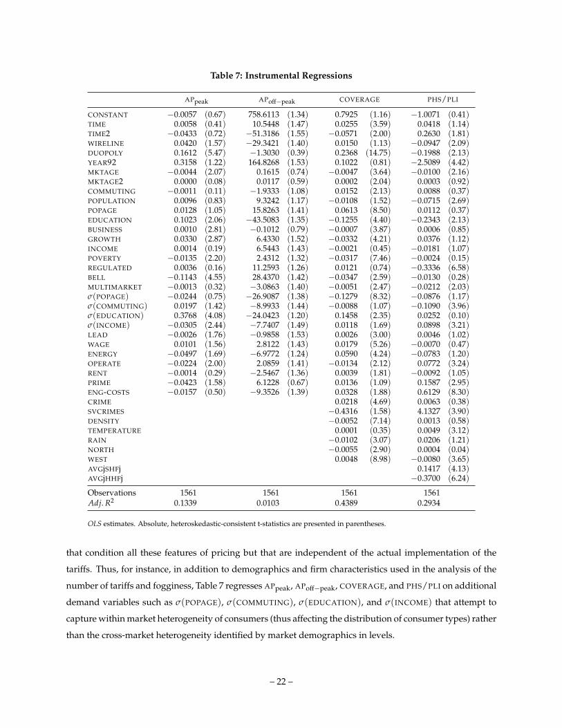
Table 7: Instrumental Regressions

APpeak APoff−peak COVERAGE PHS/PLI

CONSTANT −0.0057 (0.67) 758.6113 (1.34) 0.7925 (1.16) −1.0071 (0.41)TIME 0.0058 (0.41) 10.5448 (1.47) 0.0255 (3.59) 0.0418 (1.14)TIME2 −0.0433 (0.72) −51.3186 (1.55) −0.0571 (2.00) 0.2630 (1.81)WIRELINE 0.0420 (1.57) −29.3421 (1.40) 0.0150 (1.13) −0.0947 (2.09)DUOPOLY 0.1612 (5.47) −1.3030 (0.39) 0.2368 (14.75) −0.1988 (2.13)YEAR92 0.3158 (1.22) 164.8268 (1.53) 0.1022 (0.81) −2.5089 (4.42)MKTAGE −0.0044 (2.07) 0.1615 (0.74) −0.0047 (3.64) −0.0100 (2.16)MKTAGE2 0.0000 (0.08) 0.0117 (0.59) 0.0002 (2.04) 0.0003 (0.92)COMMUTING −0.0011 (0.11) −1.9333 (1.08) 0.0152 (2.13) 0.0088 (0.37)POPULATION 0.0096 (0.83) 9.3242 (1.17) −0.0108 (1.52) −0.0715 (2.69)POPAGE 0.0128 (1.05) 15.8263 (1.41) 0.0613 (8.50) 0.0112 (0.37)EDUCATION 0.1023 (2.06) −43.5083 (1.35) −0.1255 (4.40) −0.2343 (2.13)BUSINESS 0.0010 (2.81) −0.1012 (0.79) −0.0007 (3.87) 0.0006 (0.85)GROWTH 0.0330 (2.87) 6.4330 (1.52) −0.0332 (4.21) 0.0376 (1.12)INCOME 0.0014 (0.19) 6.5443 (1.43) −0.0021 (0.45) −0.0181 (1.07)POVERTY −0.0135 (2.20) 2.4312 (1.32) −0.0317 (7.46) −0.0024 (0.15)REGULATED 0.0036 (0.16) 11.2593 (1.26) 0.0121 (0.74) −0.3336 (6.58)BELL −0.1143 (4.55) 28.4370 (1.42) −0.0347 (2.59) −0.0130 (0.28)MULTIMARKET −0.0013 (0.32) −3.0863 (1.40) −0.0051 (2.47) −0.0212 (2.03)σ(POPAGE) −0.0244 (0.75) −26.9087 (1.38) −0.1279 (8.32) −0.0876 (1.17)σ(COMMUTING) 0.0197 (1.42) −8.9933 (1.44) −0.0088 (1.07) −0.1090 (3.96)σ(EDUCATION) 0.3768 (4.08) −24.0423 (1.20) 0.1458 (2.35) 0.0252 (0.10)σ(INCOME) −0.0305 (2.44) −7.7407 (1.49) 0.0118 (1.69) 0.0898 (3.21)LEAD −0.0026 (1.76) −0.9858 (1.53) 0.0026 (3.00) 0.0046 (1.02)WAGE 0.0101 (1.56) 2.8122 (1.43) 0.0179 (5.26) −0.0070 (0.47)ENERGY −0.0497 (1.69) −6.9772 (1.24) 0.0590 (4.24) −0.0783 (1.20)OPERATE −0.0224 (2.00) 2.0859 (1.41) −0.0134 (2.12) 0.0772 (3.24)RENT −0.0014 (0.29) −2.5467 (1.36) 0.0039 (1.81) −0.0092 (1.05)PRIME −0.0423 (1.58) 6.1228 (0.67) 0.0136 (1.09) 0.1587 (2.95)ENG-COSTS −0.0157 (0.50) −9.3526 (1.39) 0.0328 (1.88) 0.6129 (8.30)CRIME 0.0218 (4.69) 0.0063 (0.38)SVCRIMES −0.4316 (1.58) 4.1327 (3.90)DENSITY −0.0052 (7.14) 0.0013 (0.58)TEMPERATURE 0.0001 (0.35) 0.0049 (3.12)RAIN −0.0102 (3.07) 0.0206 (1.21)NORTH −0.0055 (2.90) 0.0004 (0.04)WEST 0.0048 (8.98) −0.0080 (3.65)AVGjSHFj 0.1417 (4.13)AVGjHHFj −0.3700 (6.24)

Observations 1561 1561 1561 1561Adj. R2 0.1339 0.0103 0.4389 0.2934

OLS estimates. Absolute, heteroskedastic-consistent t-statistics are presented in parentheses.

that condition all these features of pricing but that are independent of the actual implementation of the

tariffs. Thus, for instance, in addition to demographics and firm characteristics used in the analysis of the

number of tariffs and fogginess, Table 7 regresses APpeak, APoff−peak, COVERAGE, and PHS/PLI on additional

demand variables such as σ(POPAGE), σ(COMMUTING), σ(EDUCATION), and σ(INCOME) that attempt to

capture within market heterogeneity of consumers (thus affecting the distribution of consumer types) rather

than the cross-market heterogeneity identified by market demographics in levels.

– 22 –

The usual “demand shifters” include anything that may affect the distribution of unobservable

consumers’ valuations. Since data also include competing firms, it is necessary to account for firm specific

cost shifters.15 Regressions of Table 7 include a large set of market specific cost variables such as the WAGE

index of employees of the cellular industry, the PRIME lending rate in each market, an index of the cost

of ENERGY, RENT, and operating costs of running a business (OPERATE). To identify differences in costs

among carriers of a same market, I also include variables that may capture firm specific effects such as the

identity of the owner of the license, the possibility of heterogeneous levels of efficiency due to different

accumulated experience captured by LEAD, i.e., the number of months separating the entry of the wireline

and nonwireline operators, and a firm specific engineering estimate of the average operating unit costs as

appraised by an independent research company, ENG-COSTS. Finally, the MULTIMARKET indicator intends

to capture the effect on profitability and coverage that the presence of a firm in several markets may have.

While I am treating markets independently of each other, firms operating in several markets may enjoy

some important cost savings as they could perhaps consolidate some activities across markets or establish

a softer competition regime with other firms also present in several markets through multimarket contact.

The population DENSITY of a market affects not only the deployment of antennas, but also how people

interact and their need for cellular communication. Thus, this regressor is included mostly to control for

the endogeneity of market penetration as measured by COVERAGE. In addition to this variable, available

information includes other market specific variables that might affect subscription decisions, such as geo-

graphical location, weather, or crime.16

The phasing out of certain tariff options is necessarily conditioned by previous choices of how

many options to offer and their design. Contrary to current features of the tariffs, such as their degree of

fogginess or the number of tariff options in the menu, the share of current options that were already offered

in the past is, up to certain extent, predetermined by previous pricing decisions. If demand shocks are

market specific, as opposed to nationally driven, the characteristics of the tariffs of the competitors in other

markets during past periods can also be used as valid instruments as suggested by Hausman, Leonard, and

Zona (1994) and Hausman (1996). Thus, the PHS/PLI equation includes the cross-market average of the ratio

of foggy options that were the result of phasing out, AVGjSHFj, and the fogginess index of non-dominated

options corresponding to all competing firms that a particular carrier confronted in all other markets where

this carrier operated in previous periods.

15 Observe that contrary to Bresnahan (1981) and (1987) or Berry, Levinsohn, and Pakes (1995), I cannot use the characteristicsof the tariff of the competitor in other markets as valid instruments, as the tariff characteristics are indeed endogenous to the analysis.

16 Climatology and location effects on the decision to subscribe to fixed local telephony has been documented by Crandalland Waverman (2000) and Riordan (2002, §2). Similarly, there has been much speculation about the effect of crime as a driving forceto subscription to cellular services. Indeed, cellular carriers at this early stage of the industry actively played this marketing strategy.See Murray (2002, p.212-213).

– 23 –

7 Concluding Remarks

This paper provides the first evaluation of firms’ use of deceptive strategies. I make use of an almost ideal

data set in which fogginess can be precisely defined and entry of competing firms occurs exogenously in

several local and independent markets. Firms appear to successfully engage in foggy pricing aimed at

confusing consumers and profiting from their mistakes in subscribing to the tariff option that best matches

their telephone usage profile. The paper documents that these deceptive strategies are more likely to

happen in monopolistic rather than in competitive markets. Entry of a second carrier increases both the

number of effective and foggy tariff options (the latter mostly as a result of the entrant’s pricing strategy).

However, the sudden increase in the ratio of dominated to non-dominated tariff options is not sustainable

in the long run and firms end up offering simpler, more transparent options to consumers.

This sequence of events matches the predictions of theoretical models quite well of nonlinear

pricing. As the entrant cannot effectively differentiate from the incumbent, it offers foggy options. A

foggy option may profit from consumers’ mistakes while at the same time the entrant differentiates from

the incumbent through the design of the tariff itself, perhaps aiming to steal customers from the incumbent

as argued by Yang and Ye (2006). As time goes by, the increase in market coverage forces these firms

to compete more aggressively and eventually offer far simpler nonlinear tariffs. Armstrong and Vickers

(2001) and Rochet and Stole (2002) show that the in the limit, competing firms will offer identical two-part

tariffs in equilibrium.

Consistent with the features of the early U.S. cellular market described in this paper, the expected

value of foggy pricing needs to be necessarily low. Profits are temporary and foggy pricing is used only

when numerous options have already been offered to a heterogeneous clientele, thus reducing significantly

the potential profits of additional non-dominated options. Competition further reduces the sustainability

of such pricing tactics, making redundant the government oversight of firms’s strategies.

Should we conclude that the idea of foggy tactics is hollow? The evidence presented in this paper

corresponds to a particular industry in its infancy when tariffs were easy to characterize. Fogginess many

times involves the fine print of contracts and those issues never stated explicitly in incomplete contracts.

There are many ways of hiding information from consumers but not all of them are suitable to be easily

measured in a manner that it is possible to conduct a proper econometric analysis. The importance of

the results of this paper is that it documents that foggy pricing is not sustainable in the long run and

that the simplifying effect of competition can already be noticed with the entry of just a second competitor.

Results clearly favor the interpretation of foggy pricing as a short run strategy. Broadening competition will

eventually lift the fog and neither policy makers or social scientists will have to worry about the potentially

mistaken choices of consumers.

– 24 –

References

ARMSTRONG, M. AND J. VICKERS (2001): “Competitive Price Discrimination.” RAND Journal of Economics,32, 579–605.

BASALUZZO, G. AND E. J. MIRAVETE (2007): “Constrained Monopoly Pricing with Endogenous Participa-tion.” Mimeo, University of Texas at Austin.

BERRY, S., J. LEVINSOHN, AND A. PAKES (1995): “Automobile Prices in Market Equilibrium.” Econometrica,63, 841–890.

BRANDENBURGER, A. M. AND B. J. NALEBUFF (1996): Co-opetition. New York, NY: Doubleday.

BRESNAHAN, T. F. (1981): “Departures from Marginal-Cost Pricing in the American Automobile Industry.”Journal of Econometrics, 17, 201–227.

BRESNAHAN, T. F. (1987): “Competition and Collusion in the American Automobile Oligopoly: The 1955Price War.” Journal of Industrial Economics, 35, 457–482.

BUSSE, M. R. (2000): “Multimarket Contact and Price Coordination in the Cellular Telephone Industry.”Journal of Economics & Management Strategy, 9, 287–320.

BUSSE, M. R. AND M. RYSMAN (2005): “Competition and Price Discrimination in Yellow Pages Advertis-ing.” RAND Journal of Economics, 36, 378–390.

CAMERON, A. C. AND P. K. TRIVEDI (1998): Regression Analysis of Count Data. New York, NY: CambridgeUniversity Press.

CAMERON, A. C. AND F. A. G. WINDMEIJER (1996): “R-Squared Measures for Count Data RegressionModels with Applications to Health Care Utilization.” Journal of Business and Economic Statistics, 14,209–220.

CRANDALL, R. W. AND L. WAVERMAN (2000): Who Pays for “Universal Service”? When Telephone SubsidiesBecome Transparent. Washington, DC: Brookings Institution Press.

ECONOMIDES, N., K. SEIM, AND V. B. VIARD (2006): “Quantifying the Benefits of Entry into Local phoneService.” Mimeo, NYU Stern School of Business, Wharton School, and Stanford GSB.

ELLISON, G. AND S. F. ELLISON (2004): “Search, Obfuscation, and Price Elasticities on the Internet.”Working Paper 10570, NBER.

GABAIX, X. AND D. LAIBSON (2006): “Shrouded Attributes, Consumer Myopia, and Information Supres-sion in Competitive Markets.” Quarterly Journal of Economics, 121, 505–540.

GOURIEROUX, C., A. MONFORT, AND A. TROGNON (1984): “Pseudo Maximum Likelihood Methods:Applications to Poisson Models.” Econometrica, 52, 701–720.

HAUSMAN, J. (1996): “Valuation of New Goods under Perfect and Imperfect Competition.” In T. F. Bres-nahan and R. J. Gordon (eds.): The Economics of New Goods, Studies in Income and Wealth, Vol. 58.Chicago, IL: NBER–The University of Chicago Press.

HAUSMAN, J. A. (2002): “Mobile Telephone.” In M. Cave, S. K. Majumdar, and I. Vogelsang (eds.): Handbookof Telecommunications Economics, Vol. I. Amsterdam, The Netherlands: North-Holland.

HAUSMAN, J. A., G. LEONARD, AND J. D. ZONA (1994): “Competitive Analysis with Differentiated Prod-ucts.” Annales d’Economie et de Statistique, 34, 159–180.

LIEBMAN, J. B. AND R. J. ZECKHAUSER (2004): “Schmeduling.” Mimeo, Harvard University.

– 25 –

MARCIANO, S. (2000): “Pricing Policies in Oligopoly with Product Differentiation: The Case of CellularTelephony.” Ph.D. Thesis, University of Chicago Graduate School of Business.

MASKIN, E. AND J. RILEY (1984): “Monopoly with Incomplete Information.” RAND Journal of Economics,15, 171–196.

MIRAVETE, E. J. (2003): “Choosing the Wrong Calling Plan? Ignorance and Learning.” American EconomicReview, 93, 297–310.

MIRAVETE, E. J. (2005): “The Welfare Performace of Sequential Pricing Mechanisms.” International EconomicReview, 46, 1321–1360.

MURRAY, J. B., JR (2002): Wireless Nation. The Frenzied Launch of the Cellular Revolution in America. Cam-bridge, MA: Perseus Publishing.

OI, W. (1971): “A Disneyland Dilemma: Two-Part Tariffs for a Mickey Mouse Monopoly.” Quarterly Journalof Economic, 85, 77–96.

PARKER, P. M. (1990): “McCaw versus Pactel: Cellular Pricing (A).” Business Case, INSEAD-CEDEP.

PARKER, P. M. AND L.-H. RÖLLER (1997): “Collusive Conduct in Duopolies: Multimarket Contact andCross-Ownership in the Mobile Telephone Industry.” RAND Journal of Economics, 28, 304–322.

RIORDAN, M. (2002): “Universal Residential Telephone Services.” In M. E. Cave, S. K. Majumdar, andI. Vogelsang (eds.): Handbook of Telecommunications Economics, Vol. I. Amsterdam, The Netherlands:North-Holland.

ROCHET, J.-C. AND L. A. STOLE (2002): “Nonlinear Pricing with Random Participation.” The Review ofEconomic Studies, 69, 277–311.

SEIM, K. AND V. B. VIARD (2005): “The Effect of Entry and Market Structure on Cellular Pricing Tactics.”Mimeo, Stanford Graduate School of Business.

SHEW, W. B. (1994): “Regulation, Competition, and Prices in the U.S. Cellular Telephone Industry.” Mimeo,The American Enterprise Institute.

TIROLE, J. (1989): Industrial Organization. Cambridge, MA: MIT.

VOGELSANG, I. AND B. M. MITCHELL (1997): Telecommunications Competition: The Last Ten Miles. Cam-bridge, MA: AEI–MIT Press.

WILSON, R. B. (1993): Nonlinear Pricing. New York, NY: Oxford University Press.

WOOLDRIDGE, J. M. (1995): “Score Diagnostics for Linear Models Estimated by Two Stage Least Squares.”In G. S. Maddala, P. C. B. Phillips, and T. N. Srinivasan (eds.): Advances in Econometrics and Quanti-tative Economics. Oxford, UK: Blackwell.

WOOLDRIDGE, J. M. (1997): “Quasi-Likelihood Methods for Count Data.” In M. H. Pesaran and P. Schmidt(eds.): Handbook of Applied Econometrics, Vol. 2. Oxford, UK: Blackwell.

WOOLDRIDGE, J. M. (2002): Econometric Analysis of Cross Section and Panel Data. Cambridge, MA: MITPress.

YANG, H. AND L. YE (2006): “Nonlinear Pricing, Contract Variety, and Competition.” Mimeo, Ohio StateUniversity.

– 26 –

Appendix

A Definition of Variables and Description of Data Sources

• Tariff information is reported by Cellular Price and Marketing Letter, Information Enterprises, various

issues, 1984–1988. This information was collected by Economic and Management Consultants Inter-

national, Inc. For year 1992, Marciano (2000) combined information from Cellular Directions, Inc.,

the Cellular Telephone Industry Association, and direct interviews with managers. TIME indicates the

number of months since the first monopolist started offering cellular service in the U.S.; WIRELINE

identifies the owner of the first cellular license in each market; and DUOPOLY and YEAR92 are two

dummy variables that identify whether a market enjoys a competitive regime and the year 1992

observations, respectively. Finally, MKTAGE accounts for the age of each market in months (when

service was first offered by any of the two firms in each market).

• Socioeconomic and demographic data of each market come from the 1989 Statistical Abstracts of the

United States; U.S. Department of Commerce, Bureau of the Census, using the FCC Cellular Bound-

ary Notices, 1982–1987, available in The Cellular Market Data Book, EMCI, Inc.; as well as the 1990

U.S. Decennial Census. Variables include the average commuting time in minutes, COMMUTING;

thousands of high potential business establishments, BUSINESS,17 total population of the SMSA in

millions, POPULATION, the average percent growth of population in the 1980’s, GROWTH, median

income in thousands of dollars, INCOME, percentage of households with income below the poverty

level, POVERTY, median age of population in years, POPAGE, and median number of years of edu-

cation, EDUCATION. Variables marked “σ(·)” indicate the within market standard deviation of the

corresponding demographic.

• The REGULATED dummy indicates that firms were required to get approval to offer new tariffs. The

regulation regime was reported by the Cellular Telephone Industry Association in State of the Cellular

Industry, 1992.

• Largest shareholder information is available from the FCC. We identify whether it belongs to a firm

of the former BELL system.

• Industry cost indicators for each market are obtained from the Bureau of Labor Statistics; U.S. De-

partment of Energy; BOMA Experience Exchange Report: Income/Expense Analysis for Office Buildings,

various issues, 1985–1989, and Cellular Price and Marketing Letter, Information Enterprises, various

17 BUSINESS refers to what was considered at that time as highly potential customers by cellular industry experts: businessservice firms, health care, professional, and legal services, contract construction, transportation, finance, insurance, and real estate.

– 27 –

issues, 1984–1988, and 1990 U.S. Census. They include the population density of the market (people

per square mile), DENSITY, the number of months each market was served only by the incumbent firm,

LEAD, the number of markets in which a firm operates, MULTIMARKET, the state average electricity

rates in dollars per kilowatt/hour, ENERGY, one-period lagged prime lending rate, PRIME, an index of

operating expenses per square foot of office space, OPERATE,18 an index of average monthly rent per

square foot of office space in each market, RENT, and an index of average annual wages per employee

for the cellular industry, WAGE. Finally, ENG-COSTS is an engineering estimate of the average cost of

production for each firm in the sample.19

• Weather and location data are available on the web at http://cdiac.esd.ornl.org, and include average

temperature and precipitation for 1,221 stations in the contiguous continental states plus those of

Alaska.20 Data include the average quarterly temperature in Fahrenheit degrees recorded at the

closest station to each market, TEMPERATURE, and the average quarterly precipitation in inches, RAIN.

NORTH and WEST indicate the longitude and latitude of the geographical center of each SMSA in

degrees.

• Crime information is obtained from the Uniform Crime Report, FBI, 1984–1988. We include the number

of offenses per 1000 inhabitants, CRIMEand the percent share of violent crimes in each market, which

is denoted by SVCRIMES.21

• Endogenous variables include the number of tariff plans, PLANS, how many of them are actually

non-dominated, EFFPLANS, the share of total tariffs offered that are indeed dominated, SHARE-FOGGY,

and the degree of fogginess of the non-dominated options, FOGGINESS, as constructed in Section 5.

Other potentially endogenous variables are constructed, as discussed in the text, to identify relevant

information upon which firms may condition their decision to offer more or less effective and/or

dominated tariff options. These variables are curvature of the peak and off-peak tariff schedule

as defined by APpeak and APoff−peak, the ratio of total to potential subscribers, COVERAGE, and the

percentage of dominated tariff options options that were offered in previous periods, PHS/PLI.

18 These expenses include cleaning, repair and maintenance, administrative costs, utilities, local taxes, security and groundservices, office payroll, and other leasing expenses associated with running an office.

19 This indicator was provided by an independent research firm to Economic and Management Consultants International, Inc.,the firm which collected the tariff information used in this paper. See Parker (1990).

20 See Easterling, D.R., T.R. Karl, EH. Mason, P.Y. Hughes, D.P. Bowman and R.C. Daniels, United States Historical ClimatologyNetwork (U.S. HCN) Monthly Temperature and Precipitation Data. ORNL/CDIAC-87, NDP-019/R3, 1996. Carbon Dioxide InformationAnalysis Center, Oak Ridge National Laboratory, Oak Ridge, Tennessee.

21 Violent offenses include murder, non-negligent manslaughter, forcible rape, robbery, and aggravated assault. Propertyoffenses include burglary, larceny-theft, motor vehicle theft, and arson.

– 28 –

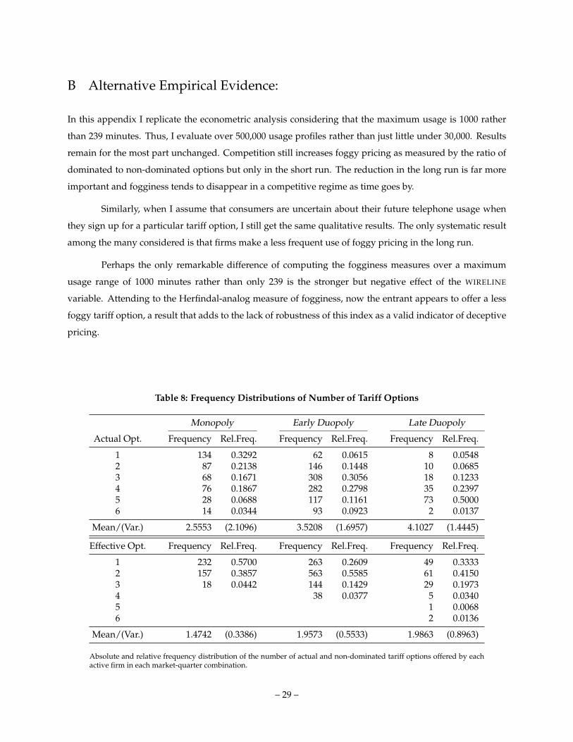
B Alternative Empirical Evidence:

In this appendix I replicate the econometric analysis considering that the maximum usage is 1000 rather

than 239 minutes. Thus, I evaluate over 500,000 usage profiles rather than just little under 30,000. Results

remain for the most part unchanged. Competition still increases foggy pricing as measured by the ratio of

dominated to non-dominated options but only in the short run. The reduction in the long run is far more

important and fogginess tends to disappear in a competitive regime as time goes by.

Similarly, when I assume that consumers are uncertain about their future telephone usage when

they sign up for a particular tariff option, I still get the same qualitative results. The only systematic result

among the many considered is that firms make a less frequent use of foggy pricing in the long run.

Perhaps the only remarkable difference of computing the fogginess measures over a maximum

usage range of 1000 minutes rather than only 239 is the stronger but negative effect of the WIRELINE

variable. Attending to the Herfindal-analog measure of fogginess, now the entrant appears to offer a less

foggy tariff option, a result that adds to the lack of robustness of this index as a valid indicator of deceptive

pricing.

Table 8: Frequency Distributions of Number of Tariff Options

Monopoly Early Duopoly Late Duopoly

Actual Opt. Frequency Rel.Freq. Frequency Rel.Freq. Frequency Rel.Freq.

1 134 0.3292 62 0.0615 8 0.05482 87 0.2138 146 0.1448 10 0.06853 68 0.1671 308 0.3056 18 0.12334 76 0.1867 282 0.2798 35 0.23975 28 0.0688 117 0.1161 73 0.50006 14 0.0344 93 0.0923 2 0.0137

Mean/(Var.) 2.5553 (2.1096) 3.5208 (1.6957) 4.1027 (1.4445)

Effective Opt. Frequency Rel.Freq. Frequency Rel.Freq. Frequency Rel.Freq.

1 232 0.5700 263 0.2609 49 0.33332 157 0.3857 563 0.5585 61 0.41503 18 0.0442 144 0.1429 29 0.19734 38 0.0377 5 0.03405 1 0.00686 2 0.0136

Mean/(Var.) 1.4742 (0.3386) 1.9573 (0.5533) 1.9863 (0.8963)

Absolute and relative frequency distribution of the number of actual and non-dominated tariff options offered by eachactive firm in each market-quarter combination.

– 29 –

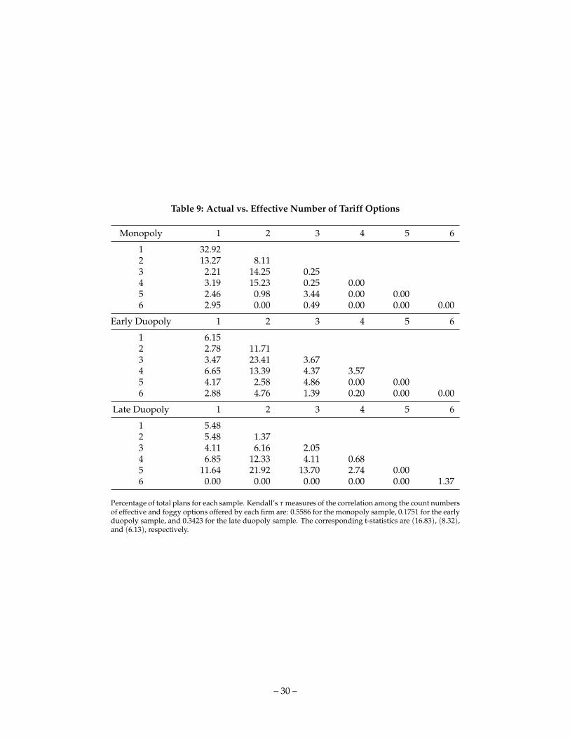
Table 9: Actual vs. Effective Number of Tariff Options

Monopoly 1 2 3 4 5 6

1 32.922 13.27 8.113 2.21 14.25 0.254 3.19 15.23 0.25 0.005 2.46 0.98 3.44 0.00 0.006 2.95 0.00 0.49 0.00 0.00 0.00

Early Duopoly 1 2 3 4 5 6

1 6.152 2.78 11.713 3.47 23.41 3.674 6.65 13.39 4.37 3.575 4.17 2.58 4.86 0.00 0.006 2.88 4.76 1.39 0.20 0.00 0.00

Late Duopoly 1 2 3 4 5 6

1 5.482 5.48 1.373 4.11 6.16 2.054 6.85 12.33 4.11 0.685 11.64 21.92 13.70 2.74 0.006 0.00 0.00 0.00 0.00 0.00 1.37

Percentage of total plans for each sample. Kendall’s τ measures of the correlation among the count numbersof effective and foggy options offered by each firm are: 0.5586 for the monopoly sample, 0.1751 for the earlyduopoly sample, and 0.3423 for the late duopoly sample. The corresponding t-statistics are (16.83), (8.32),and (6.13), respectively.

– 30 –

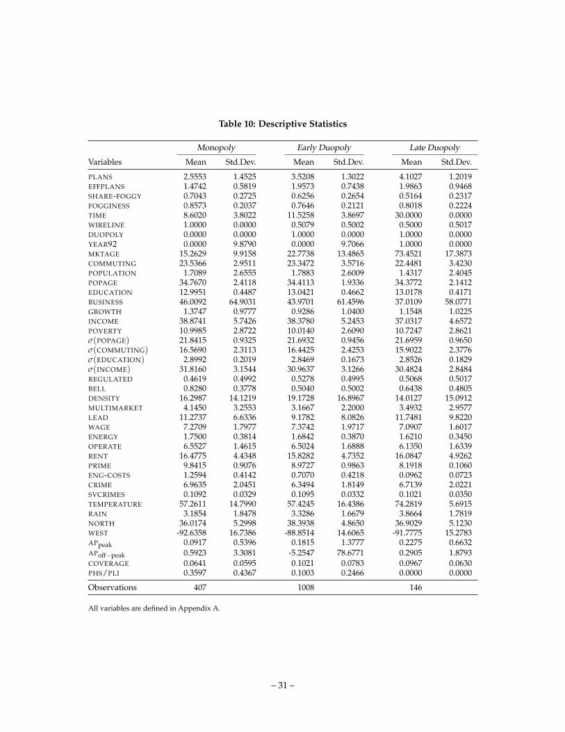
Table 10: Descriptive Statistics

Monopoly Early Duopoly Late Duopoly

Variables Mean Std.Dev. Mean Std.Dev. Mean Std.Dev.

PLANS 2.5553 1.4525 3.5208 1.3022 4.1027 1.2019EFFPLANS 1.4742 0.5819 1.9573 0.7438 1.9863 0.9468SHARE-FOGGY 0.7043 0.2725 0.6256 0.2654 0.5164 0.2317FOGGINESS 0.8573 0.2037 0.7646 0.2121 0.8018 0.2224TIME 8.6020 3.8022 11.5258 3.8697 30.0000 0.0000WIRELINE 1.0000 0.0000 0.5079 0.5002 0.5000 0.5017DUOPOLY 0.0000 0.0000 1.0000 0.0000 1.0000 0.0000YEAR92 0.0000 9.8790 0.0000 9.7066 1.0000 0.0000MKTAGE 15.2629 9.9158 22.7738 13.4865 73.4521 17.3873COMMUTING 23.5366 2.9511 23.3472 3.5716 22.4481 3.4230POPULATION 1.7089 2.6555 1.7883 2.6009 1.4317 2.4045POPAGE 34.7670 2.4118 34.4113 1.9336 34.3772 2.1412EDUCATION 12.9951 0.4487 13.0421 0.4662 13.0178 0.4171BUSINESS 46.0092 64.9031 43.9701 61.4596 37.0109 58.0771GROWTH 1.3747 0.9777 0.9286 1.0400 1.1548 1.0225INCOME 38.8741 5.7426 38.3780 5.2453 37.0317 4.6572POVERTY 10.9985 2.8722 10.0140 2.6090 10.7247 2.8621σ(POPAGE) 21.8415 0.9325 21.6932 0.9456 21.6959 0.9650σ(COMMUTING) 16.5690 2.3113 16.4425 2.4253 15.9022 2.3776σ(EDUCATION) 2.8992 0.2019 2.8469 0.1673 2.8526 0.1829σ(INCOME) 31.8160 3.1544 30.9637 3.1266 30.4824 2.8484REGULATED 0.4619 0.4992 0.5278 0.4995 0.5068 0.5017BELL 0.8280 0.3778 0.5040 0.5002 0.6438 0.4805DENSITY 16.2987 14.1219 19.1728 16.8967 14.0127 15.0912MULTIMARKET 4.1450 3.2553 3.1667 2.2000 3.4932 2.9577LEAD 11.2737 6.6336 9.1782 8.0826 11.7481 9.8220WAGE 7.2709 1.7977 7.3742 1.9717 7.0907 1.6017ENERGY 1.7500 0.3814 1.6842 0.3870 1.6210 0.3450OPERATE 6.5527 1.4615 6.5024 1.6888 6.1350 1.6339RENT 16.4775 4.4348 15.8282 4.7352 16.0847 4.9262PRIME 9.8415 0.9076 8.9727 0.9863 8.1918 0.1060ENG-COSTS 1.2594 0.4142 0.7070 0.4218 0.0962 0.0723CRIME 6.9635 2.0451 6.3494 1.8149 6.7139 2.0221SVCRIMES 0.1092 0.0329 0.1095 0.0332 0.1021 0.0350TEMPERATURE 57.2611 14.7990 57.4245 16.4386 74.2819 5.6915RAIN 3.1854 1.8478 3.3286 1.6679 3.8664 1.7819NORTH 36.0174 5.2998 38.3938 4.8650 36.9029 5.1230WEST -92.6358 16.7386 -88.8514 14.6065 -91.7775 15.2783APpeak 0.0917 0.5396 0.1815 1.3777 0.2275 0.6632APoff−peak 0.5923 3.3081 -5.2547 78.6771 0.2905 1.8793COVERAGE 0.0641 0.0595 0.1021 0.0783 0.0967 0.0630PHS/PLI 0.3597 0.4367 0.1003 0.2466 0.0000 0.0000

Observations 407 1008 146

All variables are defined in Appendix A.

– 31 –

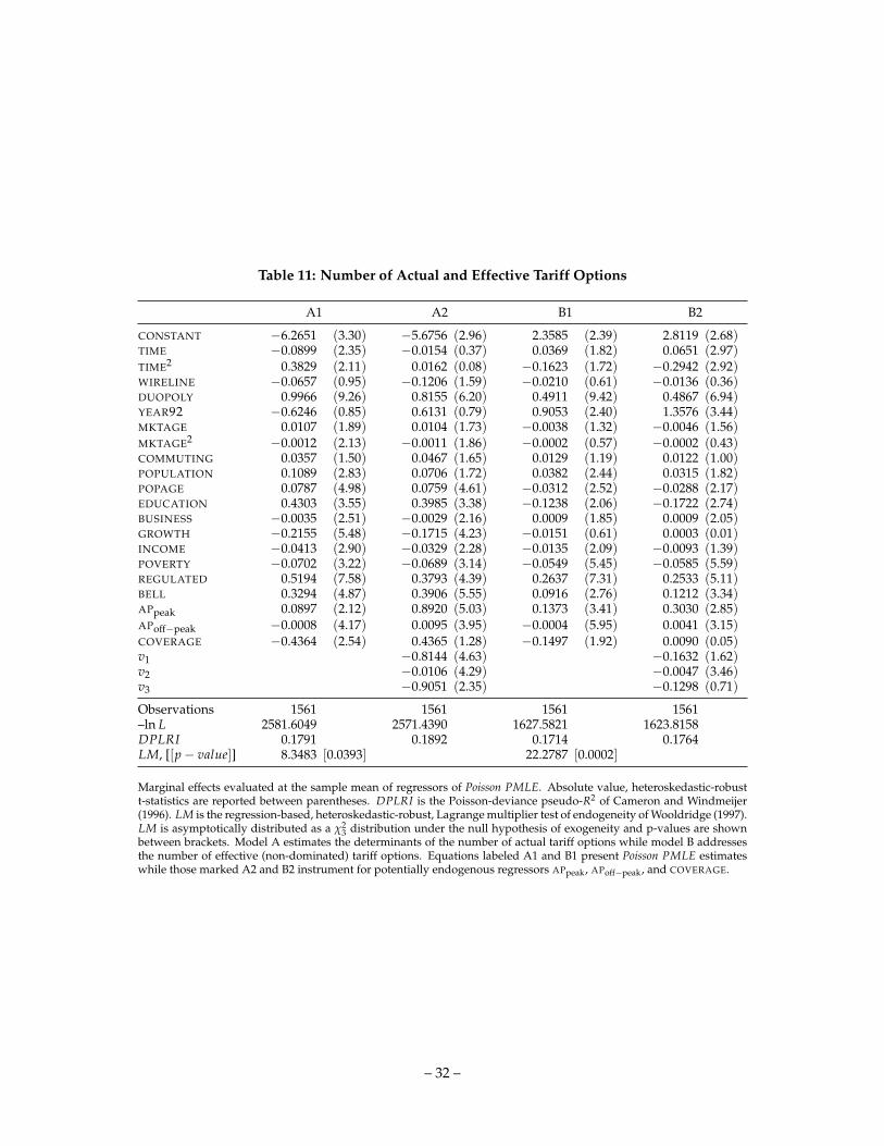
Table 11: Number of Actual and Effective Tariff Options

A1 A2 B1 B2

CONSTANT −6.2651 (3.30) −5.6756 (2.96) 2.3585 (2.39) 2.8119 (2.68)TIME −0.0899 (2.35) −0.0154 (0.37) 0.0369 (1.82) 0.0651 (2.97)TIME2 0.3829 (2.11) 0.0162 (0.08) −0.1623 (1.72) −0.2942 (2.92)WIRELINE −0.0657 (0.95) −0.1206 (1.59) −0.0210 (0.61) −0.0136 (0.36)DUOPOLY 0.9966 (9.26) 0.8155 (6.20) 0.4911 (9.42) 0.4867 (6.94)YEAR92 −0.6246 (0.85) 0.6131 (0.79) 0.9053 (2.40) 1.3576 (3.44)MKTAGE 0.0107 (1.89) 0.0104 (1.73) −0.0038 (1.32) −0.0046 (1.56)MKTAGE2 −0.0012 (2.13) −0.0011 (1.86) −0.0002 (0.57) −0.0002 (0.43)COMMUTING 0.0357 (1.50) 0.0467 (1.65) 0.0129 (1.19) 0.0122 (1.00)POPULATION 0.1089 (2.83) 0.0706 (1.72) 0.0382 (2.44) 0.0315 (1.82)POPAGE 0.0787 (4.98) 0.0759 (4.61) −0.0312 (2.52) −0.0288 (2.17)EDUCATION 0.4303 (3.55) 0.3985 (3.38) −0.1238 (2.06) −0.1722 (2.74)BUSINESS −0.0035 (2.51) −0.0029 (2.16) 0.0009 (1.85) 0.0009 (2.05)GROWTH −0.2155 (5.48) −0.1715 (4.23) −0.0151 (0.61) 0.0003 (0.01)INCOME −0.0413 (2.90) −0.0329 (2.28) −0.0135 (2.09) −0.0093 (1.39)POVERTY −0.0702 (3.22) −0.0689 (3.14) −0.0549 (5.45) −0.0585 (5.59)REGULATED 0.5194 (7.58) 0.3793 (4.39) 0.2637 (7.31) 0.2533 (5.11)BELL 0.3294 (4.87) 0.3906 (5.55) 0.0916 (2.76) 0.1212 (3.34)APpeak 0.0897 (2.12) 0.8920 (5.03) 0.1373 (3.41) 0.3030 (2.85)APoff−peak −0.0008 (4.17) 0.0095 (3.95) −0.0004 (5.95) 0.0041 (3.15)COVERAGE −0.4364 (2.54) 0.4365 (1.28) −0.1497 (1.92) 0.0090 (0.05)v1 −0.8144 (4.63) −0.1632 (1.62)v2 −0.0106 (4.29) −0.0047 (3.46)v3 −0.9051 (2.35) −0.1298 (0.71)

Observations 1561 1561 1561 1561–ln L 2581.6049 2571.4390 1627.5821 1623.8158DPLRI 0.1791 0.1892 0.1714 0.1764LM, [[p − value]] 8.3483 [0.0393] 22.2787 [0.0002]

Marginal effects evaluated at the sample mean of regressors of Poisson PMLE. Absolute value, heteroskedastic-robustt-statistics are reported between parentheses. DPLRI is the Poisson-deviance pseudo-R2 of Cameron and Windmeijer(1996). LM is the regression-based, heteroskedastic-robust, Lagrange multiplier test of endogeneity of Wooldridge (1997).LM is asymptotically distributed as a χ2

3 distribution under the null hypothesis of exogeneity and p-values are shownbetween brackets. Model A estimates the determinants of the number of actual tariff options while model B addressesthe number of effective (non-dominated) tariff options. Equations labeled A1 and B1 present Poisson PMLE estimateswhile those marked A2 and B2 instrument for potentially endogenous regressors APpeak, APoff−peak, and COVERAGE.

– 32 –

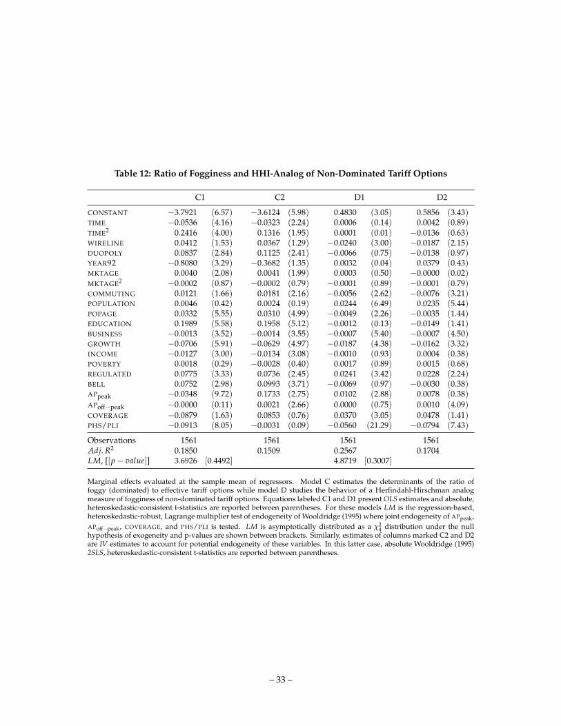
Table 12: Ratio of Fogginess and HHI-Analog of Non-Dominated Tariff Options

C1 C2 D1 D2

CONSTANT −3.7921 (6.57) −3.6124 (5.98) 0.4830 (3.05) 0.5856 (3.43)TIME −0.0536 (4.16) −0.0323 (2.24) 0.0006 (0.14) 0.0042 (0.89)TIME2 0.2416 (4.00) 0.1316 (1.95) 0.0001 (0.01) −0.0136 (0.63)WIRELINE 0.0412 (1.53) 0.0367 (1.29) −0.0240 (3.00) −0.0187 (2.15)DUOPOLY 0.0837 (2.84) 0.1125 (2.41) −0.0066 (0.75) −0.0138 (0.97)YEAR92 −0.8080 (3.29) −0.3682 (1.35) 0.0032 (0.04) 0.0379 (0.43)MKTAGE 0.0040 (2.08) 0.0041 (1.99) 0.0003 (0.50) −0.0000 (0.02)MKTAGE2 −0.0002 (0.87) −0.0002 (0.79) −0.0001 (0.89) −0.0001 (0.79)COMMUTING 0.0121 (1.66) 0.0181 (2.16) −0.0056 (2.62) −0.0076 (3.21)POPULATION 0.0046 (0.42) 0.0024 (0.19) 0.0244 (6.49) 0.0235 (5.44)POPAGE 0.0332 (5.55) 0.0310 (4.99) −0.0049 (2.26) −0.0035 (1.44)EDUCATION 0.1989 (5.58) 0.1958 (5.12) −0.0012 (0.13) −0.0149 (1.41)BUSINESS −0.0013 (3.52) −0.0014 (3.55) −0.0007 (5.40) −0.0007 (4.50)GROWTH −0.0706 (5.91) −0.0629 (4.97) −0.0187 (4.38) −0.0162 (3.32)INCOME −0.0127 (3.00) −0.0134 (3.08) −0.0010 (0.93) 0.0004 (0.38)POVERTY 0.0018 (0.29) −0.0028 (0.40) 0.0017 (0.89) 0.0015 (0.68)REGULATED 0.0775 (3.33) 0.0736 (2.45) 0.0241 (3.42) 0.0228 (2.24)BELL 0.0752 (2.98) 0.0993 (3.71) −0.0069 (0.97) −0.0030 (0.38)APpeak −0.0348 (9.72) 0.1733 (2.75) 0.0102 (2.88) 0.0078 (0.38)APoff−peak −0.0000 (0.11) 0.0021 (2.66) 0.0000 (0.75) 0.0010 (4.09)COVERAGE −0.0879 (1.63) 0.0853 (0.76) 0.0370 (3.05) 0.0478 (1.41)PHS/PLI −0.0913 (8.05) −0.0031 (0.09) −0.0560 (21.29) −0.0794 (7.43)

Observations 1561 1561 1561 1561Adj. R2 0.1850 0.1509 0.2567 0.1704LM, [[p − value]] 3.6926 [0.4492] 4.8719 [0.3007]

Marginal effects evaluated at the sample mean of regressors. Model C estimates the determinants of the ratio offoggy (dominated) to effective tariff options while model D studies the behavior of a Herfindahl-Hirschman analogmeasure of fogginess of non-dominated tariff options. Equations labeled C1 and D1 present OLS estimates and absolute,heteroskedastic-consistent t-statistics are reported between parentheses. For these models LM is the regression-based,heteroskedastic-robust, Lagrange multiplier test of endogeneity of Wooldridge (1995) where joint endogeneity of APpeak,APoff−peak, COVERAGE, and PHS/PLI is tested. LM is asymptotically distributed as a χ2

4 distribution under the nullhypothesis of exogeneity and p-values are shown between brackets. Similarly, estimates of columns marked C2 and D2are IV estimates to account for potential endogeneity of these variables. In this latter case, absolute Wooldridge (1995)2SLS, heteroskedastic-consistent t-statistics are reported between parentheses.

– 33 –

Table 13: Fogginess and Uncertainty: Dominated and Non-Dominated Tariff Options

DESCRIPTIVE STATISTICSSHARE-FOGGY FOGGINESS(HHI)

Early Duopoly Late Duopoly Early Duopoly Late Duopoly

Variables Mean Std.Dev. Mean Std.Dev. Mean Std.Dev. Mean Std.Dev.

σ = 0.00µ 0.6256 (0.2654) 0.5164 (0.2317) 0.7646 (0.2121) 0.8018 (0.2224)σ = 0.10µ 0.6275 (0.2641) 0.5219 (0.2325) 0.7689 (0.2079) 0.7985 (0.2262)σ = 0.25µ 0.6360 (0.2606) 0.5332 (0.2325) 0.7776 (0.2015) 0.7933 (0.2352)σ = 0.50µ 0.6465 (0.2567) 0.5501 (0.2413) 0.7836 (0.2046) 0.7949 (0.2307)σ = 1.00µ 0.6409 (0.2545) 0.5513 (0.2400) 0.7887 (0.2108) 0.7964 (0.2254)σ = 1.50µ 0.6516 (0.2628) 0.5796 (0.2446) 0.8010 (0.1960) 0.7984 (0.2197)σ = 2.25µ 0.6423 (0.2679) 0.5924 (0.2508) 0.8070 (0.1945) 0.8021 (0.2167)σ = 3.00µ 0.6036 (0.2545) 0.6008 (0.2494) 0.8032 (0.1952) 0.7788 (0.2248)

ESTIMATESC1 C2 D1 D2

TIMEσ = 0.00µ −0.0536 (4.16) −0.0323 (2.24) 0.0006 (0.14) 0.0042 (0.89)σ = 0.10µ −0.0537 (4.18) −0.0313 (2.17) 0.0003 (0.08) 0.0033 (0.68)σ = 0.25µ −0.0510 (4.12) −0.0327 (2.33) 0.0003 (0.08) 0.0068 (1.33)σ = 0.50µ −0.0599 (5.13) −0.0469 (3.49) 0.0029 (0.66) 0.0121 (2.26)σ = 1.00µ −0.0581 (4.91) −0.0386 (2.88) −0.0013 (0.33) 0.0059 (1.14)σ = 1.50µ −0.0590 (4.11) −0.0446 (2.86) 0.0027 (0.60) 0.0100 (1.83)σ = 2.25µ −0.0659 (4.58) −0.0395 (2.54) 0.0095 (2.08) 0.0092 (1.72)σ = 3.00µ −0.0526 (3.59) −0.0294 (1.83) 0.0105 (2.75) 0.0052 (1.12)

WIRELINEσ = 0.00µ 0.0412 (1.53) 0.0367 (1.29) −0.0240 (3.00) −0.0187 (2.15)σ = 0.10µ 0.0510 (1.91) 0.0454 (1.60) −0.0297 (3.61) −0.0249 (2.80)σ = 0.25µ 0.0202 (0.76) 0.0251 (0.87) −0.0097 (1.08) −0.0104 (1.06)σ = 0.50µ 0.0487 (1.89) 0.0459 (1.65) −0.0052 (0.56) −0.0055 (0.54)σ = 1.00µ 0.0151 (0.57) 0.0218 (0.78) 0.0278 (3.19) 0.0224 (2.25)σ = 1.50µ −0.0034 (0.13) 0.0025 (0.09) 0.0148 (1.61) 0.0110 (1.03)σ = 2.25µ 0.0333 (1.21) 0.0353 (1.19) −0.0131 (1.42) −0.0129 (1.24)σ = 3.00µ −0.0139 (0.49) −0.0123 (0.40) −0.0110 (1.37) −0.0168 (1.81)

DUOPOLYσ = 0.00µ 0.0837 (2.84) 0.1125 (2.41) −0.0066 (0.75) −0.0138 (0.97)σ = 0.10µ 0.0804 (2.73) 0.1117 (2.39) −0.0132 (1.47) −0.0204 (1.43)σ = 0.25µ 0.0962 (3.34) 0.1435 (3.20) −0.0057 (0.57) −0.0182 (1.16)σ = 0.50µ 0.1229 (4.26) 0.1627 (3.72) −0.0021 (0.19) −0.0105 (0.64)σ = 1.00µ 0.0902 (3.14) 0.1434 (3.29) 0.0313 (3.27) 0.0281 (1.83)σ = 1.50µ 0.0550 (1.66) 0.1181 (2.47) 0.0472 (4.39) 0.0308 (1.78)σ = 2.25µ 0.1050 (3.12) 0.2019 (4.31) 0.0233 (2.25) −0.0092 (0.58)σ = 3.00µ 0.1181 (3.39) 0.1648 (3.43) −0.0001 (0.01) −0.0282 (2.09)

YEAR92σ = 0.00µ −0.8080 (3.29) −0.3682 (1.35) 0.0032 (0.04) 0.0379 (0.43)σ = 0.10µ −0.7845 (3.20) −0.3335 (1.23) −0.0093 (0.12) 0.0140 (0.16)σ = 0.25µ −0.7164 (2.95) −0.3553 (1.33) 0.0143 (0.17) 0.0837 (0.87)σ = 0.50µ −0.8677 (3.71) −0.6138 (2.37) 0.1072 (1.28) 0.2177 (2.20)σ = 1.00µ −0.7332 (3.14) −0.3736 (1.46) 0.0468 (0.61) 0.1304 (1.37)σ = 1.50µ −0.8462 (3.22) −0.6108 (2.12) 0.1353 (1.60) 0.2232 (2.23)σ = 2.25µ −0.8846 (3.30) −0.4405 (1.53) 0.2004 (2.34) 0.1630 (1.65)σ = 3.00µ −0.7169 (2.65) −0.4019 (1.35) 0.1437 (1.92) 0.0343 (0.39)

Marginal effects evaluated at the sample mean of regressors for samples with alternative definitions of fogginess depend-ing on the dispersion of actual calls relative to the expected telephone usage. Model C estimates the determinants of theratio of foggy (dominated) to effective tariff options while model D studies the behavior of a Herfindahl-Hirschmananalog measure of fogginess of non-dominated tariff options. Equations labeled C1 and D1 present OLS estimates andabsolute, heteroskedastic-consistent t-statistics are reported between parentheses. Similarly, estimates of columns C2and D2 are IV estimates to account for potential endogeneity of these variables. In this latter case, absolute Wooldridge(1995) 2SLS, heteroskedastic-consistent t-statistics are reported between parentheses.

– 34 –

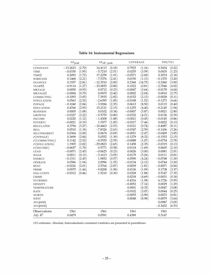
Table 14: Instrumental Regressions

APpeak APoff−peak COVERAGE PHS/PLI

CONSTANT −13.2623 (2.70) 14.4113 (0.18) 0.7925 (1.16) 0.5434 (0.22)TIME −0.0330 (1.95) −5.7210 (2.51) 0.0255 (3.59) 0.0435 (1.23)TIME2 0.2093 (1.72) 17.2259 (1.91) −0.0571 (2.00) 0.3074 (2.18)WIRELINE 0.1468 (2.21) −7.5376 (2.41) 0.0150 (1.13) −0.1370 (3.20)DUOPOLY 0.1557 (2.81) −12.3510 (2.85) 0.2368 (14.75) −0.3360 (3.90)YEAR92 −0.9114 (1.27) −33.0835 (0.80) 0.1022 (0.81) −2.7046 (4.92)MKTAGE 0.0050 (0.93) 0.0712 (0.23) −0.0047 (3.64) −0.0178 (4.04)MKTAGE2 −0.0004 (0.70) 0.0070 (0.40) 0.0002 (2.04) 0.0010 (2.75)COMMUTING −0.1093 (3.05) 7.3935 (2.82) 0.0152 (2.13) −0.0028 (0.11)POPULATION 0.0563 (2.52) −2.6395 (1.85) −0.0108 (1.52) −0.1273 (4.66)POPAGE −0.1040 (2.84) −3.9284 (2.35) 0.0613 (8.50) 0.0115 (0.40)EDUCATION 0.4766 (2.95) 15.2121 (2.15) −0.1255 (4.40) −0.2145 (1.94)BUSINESS 0.0005 (1.08) 0.0102 (0.34) −0.0007 (3.87) 0.0021 (2.80)GROWTH −0.0327 (2.22) −0.5755 (0.80) −0.0332 (4.21) 0.0136 (0.39)INCOME 0.0220 (1.12) −1.4308 (1.88) −0.0021 (0.45) −0.0145 (0.86)POVERTY −0.0021 (0.19) 1.7077 (1.85) −0.0317 (7.46) 0.0022 (0.13)REGULATED 0.3794 (3.27) −10.4463 (2.53) 0.0121 (0.74) −0.4087 (8.11)BELL 0.0510 (1.18) −7.8326 (2.63) −0.0347 (2.59) −0.1436 (3.26)MULTIMARKET 0.0364 (2.00) 0.0674 (0.09) −0.0051 (2.47) −0.0409 (3.85)σ(POPAGE) 0.3699 (2.84) 5.0552 (1.39) −0.1279 (8.32) −0.1553 (2.15)σ(COMMUTING) 0.1142 (2.52) −8.5555 (2.59) −0.0088 (1.07) −0.0754 (2.78)σ(EDUCATION) 1.1905 (2.82) −29.0823 (2.65) 0.1458 (2.35) −0.0319 (0.13)σ(INCOME) −0.0657 (1.70) 0.5771 (0.58) 0.0118 (1.69) 0.0605 (2.10)LEAD −0.0071 (2.45) −0.0625 (0.23) 0.0026 (3.00) 0.0081 (2.01)WAGE 0.0011 (0.13) −3.1613 (3.05) 0.0179 (5.26) 0.0111 (0.81)ENERGY −0.1311 (2.45) 1.9852 (0.57) 0.0590 (4.24) −0.0748 (1.30)OPERATE 0.0586 (1.94) 2.0996 (1.55) −0.0134 (2.12) 0.0744 (3.20)RENT −0.0226 (2.01) 2.5764 (2.87) 0.0039 (1.81) −0.0071 (0.84)PRIME 0.0975 (1.44) −9.8208 (1.90) 0.0136 (1.09) 0.1738 (3.37)ENG-COSTS −0.0312 (0.46) 1.5210 (0.30) 0.0328 (1.88) 0.5147 (7.35)CRIME 0.0218 (4.69) −0.0031 (0.18)SVCRIMES −0.4316 (1.58) 6.1726 (5.95)DENSITY −0.0052 (7.14) 0.0029 (1.29)TEMPERATURE 0.0001 (0.35) 0.0047 (3.08)RAIN −0.0102 (3.07) 0.0044 (0.25)NORTH −0.0055 (2.90) 0.0072 (0.81)WEST 0.0048 (8.98) −0.0079 (3.64)AVGjSHFj 0.0987 (3.05)AVGjHHFj −0.3432 (6.53)

Observations 1561 1561 1561 1561Adj. R2 0.0479 0.0591 0.4389 0.3147

OLS estimates. Absolute, heteroskedastic-consistent t-statistics are presented in parentheses.

– 35 –