The Drift Diffusion Model can account for the accuracy … and Decision Making, Vol. 5, No. 6, October 2010, pp. 437–449 The Drift Diffusion Model can account for the accuracy and

Judgment and Decision Making, Vol. 5, No. 6, October 2010, pp. 437–449

The Drift Diffusion Model can account for the accuracy andreaction time of value-based choices under high and low time

pressure

Milica Milosavljevic∗1, Jonathan Malmaud1,2∗, Alexander Huth1∗,Christof Koch1,2,3, and Antonio Rangel1,4

1 Computation and Neural Systems, California Institute of Technology, Pasadena, CA2 Division of Biology, California Institute of Technology, Pasadena, CA

3 Division of Engineering and Applied Science, California Institute of Technology, Pasadena, CA4 Division of Humanities and Social Sciences, California Institute of Technology, Pasadena, CA

Abstract

An important open problem is how values are compared to make simple choices. A natural hypothesis is that thebrain carries out the computations associated with the value comparisons in a manner consistent with the Drift DiffusionModel (DDM), since this model has been able to account for a large amount of data in other domains. We investigatedthe ability of four different versions of the DDM to explain the data in a real binary food choice task under conditionsof high and low time pressure. We found that a seven-parameter version of the DDM can account for the choice andreaction time data with high-accuracy, in both the high and low time pressure conditions. The changes associated withthe introduction of time pressure could be traced to changes in two key model parameters: the barrier height and thenoise in the slope of the drift process.

Keywords: drift-diffusion model, value-based choice, response time.

1 Introduction

The drift diffusion model (DDM) is one of the corner-stones of modern psychology (Ratcliff, 1978; Ratcliff& McKoon, 2008; Ratcliff & Smith, 2004; Smith &Ratcliff, 2004) and, increasingly, of behavioral neuro-science (Bogacz, 2007; Gold & Shadlen, 2007; Link,1992; Smith & Ratcliff, 2004). The model has receivedincreased attention over the last years for several reasons.First, it has provided more accurate descriptions of accu-racy and reaction time data than alternative models in awide range of psychological tasks, including perceptualdiscrimination and go-no-go tasks (Ratcliff & Rouder,1998, 2000; Ratcliff & Smith, 2004; Ratcliff, Van Zandt,& McKoon, 1999). Second, the model is a special caseof many of its competitors, which is a sign of its gener-ality (Bogacz, 2007; Bogacz, Brown, Moehlis, Holmes,& Cohen, 2006; Usher & McClelland, 2001). Finally,the model has been applied to explain neurophysiological

∗The first three authors contributed equally. We gratefully thank theNGA, the NSF and the Mathers and Moore Foundations for fundingthis research. We also thank Roger Ratcliff for giving us invaluablecomments during the review process.

data in various perceptual discrimination tasks (Gold &Shadlen, 2007; Heekeren, Marrett, & Ungerleider, 2008;Philiastides, Ratcliff, & Sajda, 2006; Ratcliff, Cherian, &Segraves, 2003; Ratcliff, Hasegawa, Hasegawa, Smith, &Segraves, 2007; Ratcliff, Philiastides, & Sajda, 2009) andhas a compelling neuronal interpretation.

An important open problem in behavioral neuroscienceis how the brain compares values to make simple choices.This problem is particularly interesting because there isample evidence suggesting that the comparison processis not deterministic, and that it does not always choosethe best option (Hare, Camerer, Knoepfle, O’Doherty, &Rangel, 2009; Hare, Camerer, & Rangel, 2009; Hare,O’Doherty, Camerer, Schultz, & Rangel, 2008; Padoa-Schioppa & Assad, 2006; Tom, Fox, Trepel, & Poldrack,2007). The success of the DDM in the realm of percep-tual decision making has lead several groups in neuroe-conomics to speculate that the same computational modelmight be used by the brain to make simple value basedchoices (Gold & Shadlen, 2007; Rangel, 2008; Rangel,Camerer, & Montague, 2008; Rangel & Hare, 2010; Wal-lis, 2007). This type of choice refers to situations inwhich the brain chooses among several possible stimuli

437

Judgment and Decision Making, Vol. 5, No. 6, October 2010 Diffusion model and value-based choice 438

associated with different reward values at consumption(e.g., alternative food items) by assigning a value to ev-ery item under consideration and comparing the values toselect one of them.

This paper investigates the extent to which the DDMcan explain the accuracy and reaction time data in realsimple food choices. Subjects made real choices betweenpairs of appetitive snack foods and had to eat the food thatthey chose in a randomly selected trial. This task is con-ceptually similar to previous experiments on perceptualdiscrimination (Ratcliff & Rouder, 1998) in which humansubjects had to decide which of two stimuli was bright-est. The key difference with our experiment is that oursubjects made choices between stimuli associated withdifferent levels of reward at consumption, which is aninstance of value-based choice. It is interesting to askwhether both types of tasks are described by the samecomputational model because, given the large degree ofspecialization in the brain, there is no a priori reason thatthe same algorithms would be used in the perceptual andreward domains.

We compare four different versions of the DDM thatvary in the number of free parameters that they contain,and in whether the barriers are constant or decrease withtime to speed up decision making (Cisek, Puskas, & El-Murr, 2009; Ditterich, 2006a). Since the best fittingmodel is likely to depend on the speed with which thedecisions have to be made, we carry out separate modelfitting comparisons for the two different time pressure ex-perimental conditions, which allow us to identify whichaspects of the DDM are responsible for any changes inperformance.

We found that a popular seven-parameter version of theRatcliff DDM model (Ratcliff & McKoon, 2008; Ratcliff& Rouder, 1998; Ratcliff, et al., 1999) can account forthe data with high-accuracy in both the high and low timepressure conditions. Furthermore, we also found that thechanges associated with the introduction of time pressurecould be traced to changes in two key model parameters:the barrier height and the noise in the slope of the driftprocess.

Understanding the conditions under which the DDMcan explain the behavioral data in simple value basedchoice is important for several reasons. First, it is a neces-sary first step in exploring the extent to which this modelcan account for the underlying neural computations. Sec-ond, since the DDM has been shown to provide an accu-rate description of data in other domains, the finding thatthe DDM also provides a good computational descriptionof value-based choices provides insight into the nature ofsome basic algorithms that might be at work in many dif-ferent psychological processes.

To the best of our knowledge, the performance of theDDM has not been tested before in the realm of value-

based choice, although it has been extensively tested onother realms. In fact, to the best of our knowledge, ithas provided an accurate quantitative characterization ofthe key aspects of the data in every domain to which ithas been applied. For example, the DDM has been testedin human and non-human primates using the Newsome-Shadlen random dot motion perceptual discriminationtask (Ditterich, 2006b; Mazurek, Roitman, Ditterich, &Shadlen, 2003; Philiastides, et al., 2006; Ratcliff, et al.,2003; Ratcliff, et al., 2007; Ratcliff & McKoon, 2008;Shadlen & Newsome, 2001).

A few studies have explored the ability of models re-lated to the DDM to explain various common choice pat-terns. For example, several studies have explored theability of Decision Field Theory, which is a variant of theDDM, to account for patterns of choice in multi-attributesettings such as choices among lotteries, but have notprovided a full experimental test against the data (Buse-meyer, Jessup, Johnson, & Townsend, 2006; Busemeyer& Johnson, 2004). Other studies have investigated theability of the Competing Accumulator Model to accom-plish similar goals (Usher & McClelland, 2001, 2004).Although these previous studies have shown that rela-tively simple computational models of decision-makingcan account for some stylized facts of the behavioral lit-erature, their full properties in the realm of simple valuebased choice have not been investigated.

1.1 The Drift Diffusion Model and its vari-ants

We compare the following four versions of the DDMmodel.

First, we consider the simple DDM (sDDM), which isillustrated in Figure 1A. At every instant, the model en-codes a relative value signal that measures the accumu-lated “evidence” in favor of the hypothesis that the itempresented on the left has a higher value than the item onthe right (positive values indicate that the left item is bet-ter; negative values indicate the opposite). The left itemis chosen when the relative value signal crosses the upperbarrier; the right item is chosen when the lower barrier iscrossed. The relative value signal (RVS) evolves accord-ing to the equation

X(t) = X(t− 1) + µ + ε(t),

where the drift rate µ denotes the speed at which the bar-riers are approached, and ε(t) represents white Gaussiannoise centered at zero with constant variance σ. Note thatµ + ε(t) measures the local change in the RVS signal infavor of the left alternative at the instant t. We assumethat the RVS begins the integration process with a valueof zero.


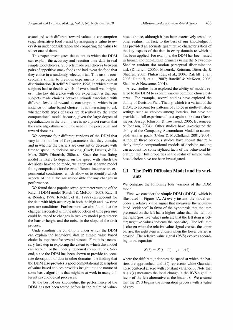
Figure 1: A) Schematic representation of the simple Dif-fusion Decision Model (sDDM) with three parameters.B) Schematic representation the simple DDM with barri-ers that decay exponentially towards 0 with time.A

B

The drift rate is a function of the value differences be-tween the left and right items, which we denote by d.In most of the estimation exercises we assume that thisfunction is linear, but we also show that this assumptionis consistent with our data.

The sDDM is characterized by the following four pa-rameters: (1) the symmetric location of the barriers (±b),(2) the linear slope of the drift rate dm (so that in any trialµ = dm · (vleft − vright), where vleft, vright denotesthe value of the items), (3) the variance of the diffusionprocess σ, and (4) a fixed latency time Tm that measuresa fixed amount of time out of every trial that takes placeprior to the initiation of the comparison process (i.e., thetime that passes from the appearance of the items and thebeginning of the DDM computations) and after the con-clusion of the process (e.g., the time that it takes to ex-ecute the motor commands necessary to implement thechoice of the DDM). It can be shown that, without loss ofgenerality, the variance parameter can be fixed, since theslope and barrier location are identified only up to ratiosof these parameters (Ratcliff & McKoon, 2008; Ratcliff,

et al., 1999). For this reason in the rest of the analyseswe set σ = 0.1, which is a commonly used normalization(Ratcliff & McKoon, 2008). Thus, the model has onlythree parameters that need to be estimated. This normal-ization is imposed in all of the four models.

Note several properties of the sDDM. First, althoughthe relative value signal typically moves towards the cor-rect barrier, the process has noise and thus mistakes aremade. This is illustrated in Figure 1A. Second, the fre-quency of mistakes increases with the amount of noiseand decreases with the value difference between the twoitems. Third, accuracy can be improved by increasing theamplitude of the barriers, but this comes at the cost oflonger reaction times.

Second, we consider a more complicated version of theDDM with additional parameters, which we refer to asthe full DDM (fDDM), which has been shown to pro-vide a more accurate description of reaction time distri-butions than the sDDM (Ratcliff & McKoon, 2008; Rat-cliff & Smith, 2004; Ratcliff, et al., 1999). The logic ofthe model is similar to the basic DDM except for the in-troduction of several additional parameters that providethe necessary flexibility to fit all of the moments of theresponse-time data in other experimental domains.

The fDDM is characterized by eight parameters: (1)It includes the four parameters from the sDDM, (2) astandard deviation dSD characterizing the noise withwhich the drift rate is sampled each period (so that ev-ery trial with values vleft and vright we have that d ∼N(dm · (vleft − vright), d2

SD), (3) a range Trange pa-rameter characterizing the support of a uniform distri-bution from which the initial latency of the process issampled every trial (so that every trial T ∼ U(Tm −Trange

2 , Tm + Trange

2 )), (4) a parameter zm that modelsthe mean a bias in the start point of the RVS accumula-tion process, which allows subjects to be biased towardsor away one of the two barriers, with zm > 0 denotingbiases towards the left barrier, and zm < 0 denoting bi-ases towards the right barrier, and (5) a range parameterzrange characterizing the support of a uniform distribu-tion from which the bias parameter for the start of theRDV signal is sampled every period (so that every trial,the start point of the accumulation process is X(T ) = z,with z ∼ U(zm − zrange

2 , zm + zrange

2 )).Third, we consider a version of the sDDM, which we

call the simple collapsing barrier DDM (scbDDM),which differs from the sDDM only in that the height ofthe upper and lower barriers decay exponentially towards0 with time according to the equation

b(t) = e−rt

where r ≥ 0 is a rate constant. This model collapses tothe sDDM when r = 0. It is characterized by five param-eters: the same for parameters describing the sDDM and


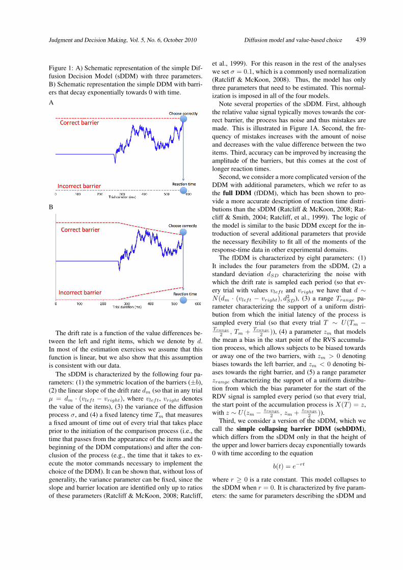
Figure 2: Sample experimental trial.

the barrier rate of decline r. The same normalization re-garding the variance described above is maintained here.

The motivation for considering time-variant decisionthresholds comes from the fact that several papers havepreviously found that they are useful in accounting forthe observation that reaction times tend to be higher inincorrect than correct trials in many psychological tasks(Churchland, Kiani, & Shadlen, 2008; Ditterich, 2006b).As shown in Figure 1B, the collapsing of the barrier canbe thought of as an urgency signal that kicks in to pre-clude the subject from taking excessively long times toreach a decision when the two items are of similar valueand thus the drift rate is close to zero. Note, however,that versions of the fDDM have been previously shownto generate slower reaction times in error trials withoutcollapsing barriers (Ratcliff & Rouder, 1998; Ratcliff, etal., 1999), which motivates one of the key questions inthe paper: how much additional explanatory power dothey provide at the expense of introducing one additionalparameter?

Fourth, we consider a version of the fDDM, which wecall the full collapsing barrier DDM (fcbDDM), whichdiffers from the fDDM only in the addition of the param-eter r measuring the rate at which the barriers collapsetowards zero.

2 MethodsSubjects. Eight Caltech students with normal or correctedto normal vision participated in two, one-hour experi-mental sessions. They were compensated $20 per ses-sion. Subjects were required not to eat for 3 hours beforethe experiment in order to increase their subjective valuefor the food items.

Experimental Task. On every trial subjects saw high-resolution color images of 50 different food items includ-ing an equal mix of salty and sweet foods (e.g., potatochips and candy bars; see Figure 2 for sample images).Items are widely available in local stores and were highlyfamiliar to our subjects. Subjects were seated in a dimlylit room with their heads positioned in a forehead andchin rest. Eye-position data were acquired from the right

eye at 1000 Hz using the Eyelink 1000 infrared eyetracker(SR Research, Osgoode, Canada). The distance betweenthe computer screen and subject was 80 cm, giving a totalvisual angle of 28º × 21º. The images were presented ona CRT screen (120 Hz) using MATLAB Psychophysicstoolbox and Eyelink toolbox extensions (Brainard, 1997;Cornelissen, Peters, & Palmer, 2002).

Each experimental session (one for each of the twoconditions described below) began with a liking-ratingtask. Subjects were shown one food item at a time, cen-tered on the monitor screen and were asked to rate howmuch they would like to eat each food item at the end ofthe experiment (−2 to 2 discrete scale). The image wasshown until subjects made a response. We used these rat-ings as independent measures of each subject’s subjectivevalue for the items.

In each condition, during the main task, subjects made750 choices between randomly selected pairs of fooditems. Figure 2 depicts the timing of the trial. Each trialbegan by requiring subjects to fixate on a central crossfor 800 ms. After the eye-tracker registered a successfulfixation, the cross disappeared leaving the blank screenfor 200 ms. Immediately after, two different food itemswere shown simultaneously for 20 ms, centered at 6.2◦

in the left and right hemifields. Next, two faint circularchoice targets were displayed at the same location as thefood items to indicate alternative saccade landing posi-tions. Subjects made a choice by fixating on the left orthe right target. A 500 ms blank screen separated the tri-als. At the end of the entire experiment subjects wererequired to eat whatever food they chose from one ran-domly selected trial, thus giving them an incentive to se-lect the highest value item of the pair on each trial. Theitems and locations were randomly selected with the con-straint that the two images should have different liking-ratings. d is the absolute value of the difference in likingrating between the two food items; in any one trial, d canbe at most 4 and is, by design, never 0. The 200 ms gapbetween fixation and food display was added because ithas been shown to accelerate saccade initiation (Fischer& Weber, 1993), which reduces the impact of motor de-lays on measured reaction times.


In order to minimize the visual demands of the task,subjects were encouraged, but not required to fixate ex-actly on the choice targets. The identity of the choice wasrecorded as soon as a saccade was initiated, as measuredby crossing a threshold located 2.2◦ from the center ofthe screen on both sides. Reaction times were measuredas the time difference between the onset of the imagesand the initiation of the saccade.

Subjects participated in two different task conditions:high and low time pressure treatments. In the low timepressure (LTP) condition they were asked to indicate theirchoice only after they were sure which item they pre-ferred. In the high time pressure (HTP) condition theywere asked to make their choices as quickly as possible.The order was counterbalanced across subjects. We se-lected these two treatments to compare the ability of theDDM to account for the data across the range of condi-tions under which consumers make decisions in the field.

Model fitting procedure. We fit the sDDM and fDDMversions of the models at the individual subject level us-ing the DMA-Toolbox (Vandekerckhove & Tuerlinckx,2008). We assumed that the slope of the drift processincreased linearly with the value difference between thetwo items (left minus right), and that the upper (lower)barrier corresponded to a left (right) choice.

Note that in this literature it is common to let the biasparameter zm to be different than zero only if there is ev-idence for either a response or a reaction time bias to oneof the two locations. This was the case in our dataset.Five subjects exhibited either a significant response biastowards left or right (binomial t-test vs. 50% null), orsignificantly different reaction times for left and right re-sponses (paired two-sided t-test).

The toolbox had to be modified to allow for the maxi-mum likelihood estimation of the scbDDM and fcbDDMversions of the models, since the original code allowedonly for constant barrier heights. Here we provide a briefdescription of the changes made to the DMA-Toolbox toaddress this problem. The modified toolbox is availablefrom the authors upon request.

As in the basic case, we assumed that that the slope ofthe drift process increased linearly with the value differ-ence between the two items (left minus right), and that theupper (lower) barrier corresponded to a left (right) choice.

Since there is no analytical formula to explicitly cal-culate the model’s predicted distribution of choice accu-racy and reaction time in the presence of collapsing barri-ers, we simulated 1000 trials using a Monte Carlo proce-dure to approximate these distributions for each candidateset of model parameters to be tested during maximum-likelihood estimation procedure. The results of the simu-lation were used to calculate the marginal probability ofmaking a correct choice, given the location of the cor-rect stimulus, and to calculate the cumulative distribution

function of the reaction time distribution conditioned onmaking a correct or incorrect choice and the location ofthe correct stimulus. The likelihood of the model wascomputed as the product of the likelihood of the individ-ual trials. The likelihood for each concrete set of parame-ters was based on the estimate of the probability of choos-ing the option chosen in that trial, as well as the proba-bility of landing on the same reaction time for that trial.Reaction time bins were given by the 5th, 10th, 30th, 50th,70th, and 90th percentiles of each subject’s reaction timedistribution.

To carry out each trial simulation, a random-walk ap-proximation to the drift diffusion process was used (Tuer-linckx, et al., 2001). At the start of each simulation, a bar-rier height, drift diffusion rate, and non-decision reactiontime were sampled according to the candidate parame-ter set, which contains the mean and variance or range ofthese quantities. A state variable representing the locationof the drift diffusion process was initialized to the biasparameter, and then updated using a time step of 10msuntil the state crossed one of the barriers using the ruledescribed below. The location of the absorbing barrier(upper or lower) was used to determine which stimuluswas chosen and hence whether this was a correct or in-correct trial, and the number of update steps needed toreach a barrier was scaled and added to the non-decisionreaction time and recorded as the net reaction time of thetrial.

In each time step of the simulation, there is a probabil-ity p that the state variable will increase by a quantity δ,and a probability (1 − p) will decrease by δ. The quan-tities p and δ are functions of the drift diffusion rate andthe time step of the simulation. They are defined so thatin the limit, as the time step approaches zero, the random-walk approximation converges to the true drift diffusionprocess. Specifically, δ is defined as σ ·√τ while p is de-fined as .5 · (1+v ·

√τ

σ ). Here, σ is the standard deviationof the noise process and is fixed at .1, τ is the time stepand is set to 10ms, and v is the drift rate for this trial.

The implementation of these changes to the DMA tool-box required two major changes. First, the module thatcalculates the probability of an observed trial given a setof model parameters was completely rewritten to use theabove procedure. Second, the optimization algorithm tofind maximum likelihood estimates in the “genalg” mod-ule of the toolbox was changed as well. By default, thismodule uses a simplex optimization procedure. However,Monte Carlo error introduces many erroneous local min-ima into the objective function and we found that simplexoptimization would often become trapped in a local min-imum. Thus, in order to increase our ability to find globalminima, we instead used a “multistart” procedure as im-plemented in the MATLAB Global Optimization toolkit.Ten candidate parameter sets were chosen approximately


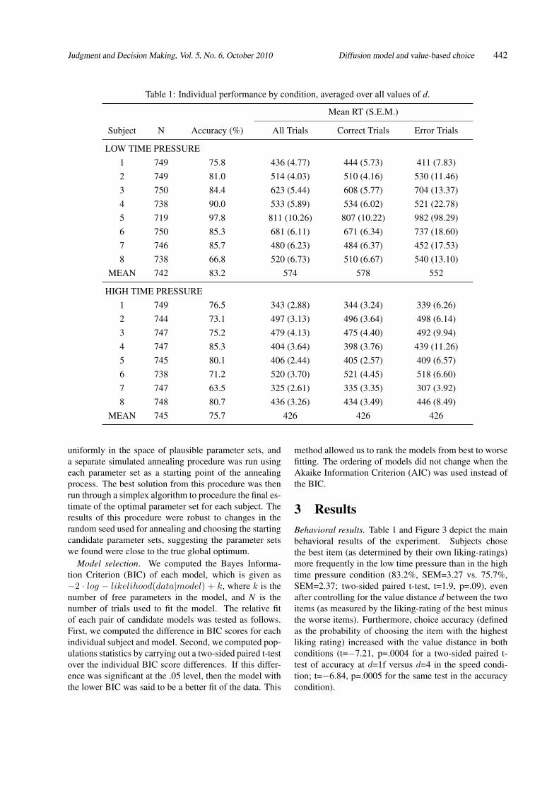
Table 1: Individual performance by condition, averaged over all values of d.

Mean RT (S.E.M.)

Subject N Accuracy (%) All Trials Correct Trials Error Trials

LOW TIME PRESSURE1 749 75.8 436 (4.77) 444 (5.73) 411 (7.83)2 749 81.0 514 (4.03) 510 (4.16) 530 (11.46)3 750 84.4 623 (5.44) 608 (5.77) 704 (13.37)4 738 90.0 533 (5.89) 534 (6.02) 521 (22.78)5 719 97.8 811 (10.26) 807 (10.22) 982 (98.29)6 750 85.3 681 (6.11) 671 (6.34) 737 (18.60)7 746 85.7 480 (6.23) 484 (6.37) 452 (17.53)8 738 66.8 520 (6.73) 510 (6.67) 540 (13.10)

MEAN 742 83.2 574 578 552

HIGH TIME PRESSURE1 749 76.5 343 (2.88) 344 (3.24) 339 (6.26)2 744 73.1 497 (3.13) 496 (3.64) 498 (6.14)3 747 75.2 479 (4.13) 475 (4.40) 492 (9.94)4 747 85.3 404 (3.64) 398 (3.76) 439 (11.26)5 745 80.1 406 (2.44) 405 (2.57) 409 (6.57)6 738 71.2 520 (3.70) 521 (4.45) 518 (6.60)7 747 63.5 325 (2.61) 335 (3.35) 307 (3.92)8 748 80.7 436 (3.26) 434 (3.49) 446 (8.49)

MEAN 745 75.7 426 426 426

uniformly in the space of plausible parameter sets, anda separate simulated annealing procedure was run usingeach parameter set as a starting point of the annealingprocess. The best solution from this procedure was thenrun through a simplex algorithm to procedure the final es-timate of the optimal parameter set for each subject. Theresults of this procedure were robust to changes in therandom seed used for annealing and choosing the startingcandidate parameter sets, suggesting the parameter setswe found were close to the true global optimum.

Model selection. We computed the Bayes Informa-tion Criterion (BIC) of each model, which is given as−2 · log − likelihood(data|model) + k, where k is thenumber of free parameters in the model, and N is thenumber of trials used to fit the model. The relative fitof each pair of candidate models was tested as follows.First, we computed the difference in BIC scores for eachindividual subject and model. Second, we computed pop-ulations statistics by carrying out a two-sided paired t-testover the individual BIC score differences. If this differ-ence was significant at the .05 level, then the model withthe lower BIC was said to be a better fit of the data. This

method allowed us to rank the models from best to worsefitting. The ordering of models did not change when theAkaike Information Criterion (AIC) was used instead ofthe BIC.

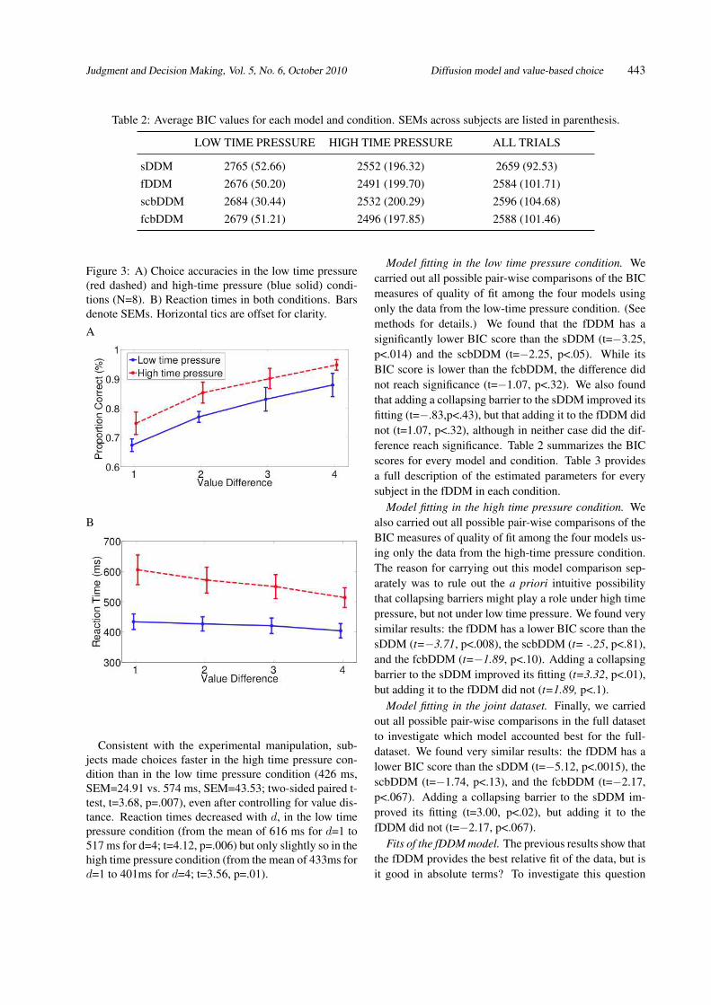
3 ResultsBehavioral results. Table 1 and Figure 3 depict the mainbehavioral results of the experiment. Subjects chosethe best item (as determined by their own liking-ratings)more frequently in the low time pressure than in the hightime pressure condition (83.2%, SEM=3.27 vs. 75.7%,SEM=2.37; two-sided paired t-test, t=1.9, p=.09), evenafter controlling for the value distance d between the twoitems (as measured by the liking-rating of the best minusthe worse items). Furthermore, choice accuracy (definedas the probability of choosing the item with the highestliking rating) increased with the value distance in bothconditions (t=−7.21, p=.0004 for a two-sided paired t-test of accuracy at d=1f versus d=4 in the speed condi-tion; t=−6.84, p=.0005 for the same test in the accuracycondition).


Table 2: Average BIC values for each model and condition. SEMs across subjects are listed in parenthesis.

LOW TIME PRESSURE HIGH TIME PRESSURE ALL TRIALS

sDDM 2765 (52.66) 2552 (196.32) 2659 (92.53)fDDM 2676 (50.20) 2491 (199.70) 2584 (101.71)scbDDM 2684 (30.44) 2532 (200.29) 2596 (104.68)fcbDDM 2679 (51.21) 2496 (197.85) 2588 (101.46)

Figure 3: A) Choice accuracies in the low time pressure(red dashed) and high-time pressure (blue solid) condi-tions (N=8). B) Reaction times in both conditions. Barsdenote SEMs. Horizontal tics are offset for clarity.A

B

Consistent with the experimental manipulation, sub-jects made choices faster in the high time pressure con-dition than in the low time pressure condition (426 ms,SEM=24.91 vs. 574 ms, SEM=43.53; two-sided paired t-test, t=3.68, p=.007), even after controlling for value dis-tance. Reaction times decreased with d, in the low timepressure condition (from the mean of 616 ms for d=1 to517 ms for d=4; t=4.12, p=.006) but only slightly so in thehigh time pressure condition (from the mean of 433ms ford=1 to 401ms for d=4; t=3.56, p=.01).

Model fitting in the low time pressure condition. Wecarried out all possible pair-wise comparisons of the BICmeasures of quality of fit among the four models usingonly the data from the low-time pressure condition. (Seemethods for details.) We found that the fDDM has asignificantly lower BIC score than the sDDM (t=−3.25,p<.014) and the scbDDM (t=−2.25, p<.05). While itsBIC score is lower than the fcbDDM, the difference didnot reach significance (t=−1.07, p<.32). We also foundthat adding a collapsing barrier to the sDDM improved itsfitting (t=−.83,p<.43), but that adding it to the fDDM didnot (t=1.07, p<.32), although in neither case did the dif-ference reach significance. Table 2 summarizes the BICscores for every model and condition. Table 3 providesa full description of the estimated parameters for everysubject in the fDDM in each condition.

Model fitting in the high time pressure condition. Wealso carried out all possible pair-wise comparisons of theBIC measures of quality of fit among the four models us-ing only the data from the high-time pressure condition.The reason for carrying out this model comparison sep-arately was to rule out the a priori intuitive possibilitythat collapsing barriers might play a role under high timepressure, but not under low time pressure. We found verysimilar results: the fDDM has a lower BIC score than thesDDM (t=−3.71, p<.008), the scbDDM (t= -.25, p<.81),and the fcbDDM (t=−1.89, p<.10). Adding a collapsingbarrier to the sDDM improved its fitting (t=3.32, p<.01),but adding it to the fDDM did not (t=1.89, p<.1).

Model fitting in the joint dataset. Finally, we carriedout all possible pair-wise comparisons in the full datasetto investigate which model accounted best for the full-dataset. We found very similar results: the fDDM has alower BIC score than the sDDM (t=−5.12, p<.0015), thescbDDM (t=−1.74, p<.13), and the fcbDDM (t=−2.17,p<.067). Adding a collapsing barrier to the sDDM im-proved its fitting (t=3.00, p<.02), but adding it to thefDDM did not (t=−2.17, p<.067).

Fits of the fDDM model. The previous results show thatthe fDDM provides the best relative fit of the data, but isit good in absolute terms? To investigate this question


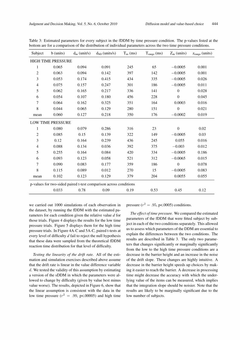
Table 3: Estimated parameters for every subject in the fDDM by time pressure condition. The p-values listed at thebottom are for a comparison of the distribution of individual parameters across the two time pressure conditions.

Subject b (units) dm (unit/s) dSD (units/s) Tm (ms) Trange (ms) Zm (units) zrange (units)

HIGH TIME PRESSURE1 0.065 0.094 0.091 245 65 −0.0005 0.0012 0.063 0.094 0.142 397 142 −0.0005 0.0013 0.053 0.174 0.415 434 335 −0.0005 0.0264 0.075 0.157 0.247 301 186 −0.0005 0.0115 0.062 0.165 0.217 336 141 0 0.0286 0.054 0.107 0.180 456 228 0 0.0457 0.064 0.162 0.325 351 164 0.0003 0.0168 0.044 0.065 0.129 280 151 0 0.021

mean 0.060 0.127 0.218 350 176 −0.0002 0.019

LOW TIME PRESSURE1 0.080 0.079 0.286 316 23 0 0.022 0.085 0.15 0.139 322 149 −0.0005 0.033 0.12 0.164 0.239 436 245 0.055 0.0164 0.088 0.134 0.036 392 375 −0.003 0.0125 0.255 0.164 0.084 420 334 −0.0005 0.1866 0.093 0.123 0.058 521 312 −0.0065 0.0157 0.090 0.083 0.177 359 186 0 0.0788 0.115 0.089 0.012 270 15 −0.0005 0.083

mean 0.102 0.123 0.129 379 204 0.0055 0.055

p-values for two-sided paired t-test comparison across conditions0.033 0.78 0.09 0.19 0.53 0.45 0.12

we carried out 1000 simulations of each observation inthe dataset, by running the fDDM with the estimated pa-rameters for each condition given the relative value d forthose trials. Figure 4 displays the results for the low timepressure trials. Figure 5 displays them for the high timepressure trials. In Figure 4A-C and 5A-C, paired t-tests atevery level of difficulty d fail to reject the null hypothesisthat these data were sampled from the theoretical fDDMreaction time distribution for that level of difficulty.

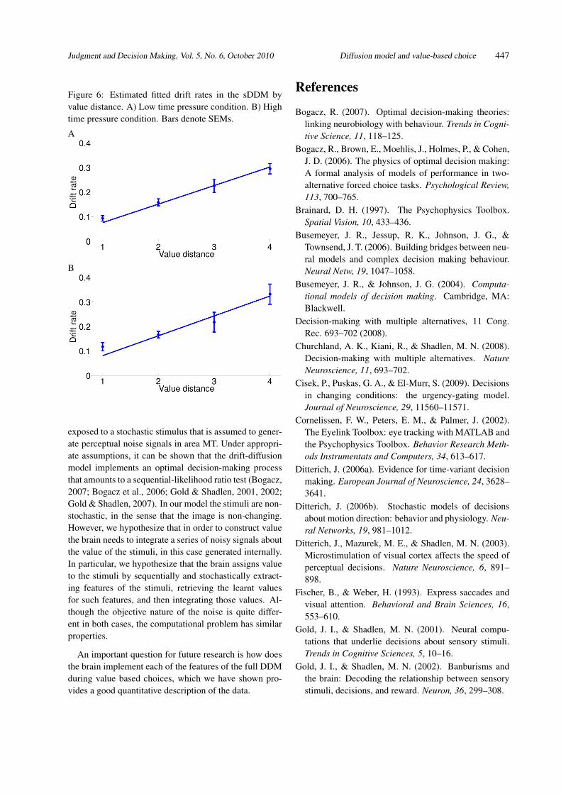
Testing the linearity of the drift rate. All of the esti-mation and simulation exercises described above assumethat the drift rate is linear in the value difference variabled. We tested the validity of this assumption by estimatinga version of the sDDM in which the parameters were al-lowed to change by difficulty (given by value best minusvalue worse). The results, depicted in Figure 6, show thatthe linear assumption is consistent with the data in thelow time pressure (r2 = .99, p<.00005) and high time

pressure (r2 = .95, p<.0005) conditions.

The effect of time pressure. We compared the estimatedparameters of the fDDM that were fitted subject by sub-ject in each of the two conditions separately. This allowedus to assess which parameters of the DDM are essential toexplain the differences between the two conditions. Theresults are described in Table 3. The only two parame-ters that changes significantly or marginally significantlyfrom the low to the high time pressure conditions are adecrease in the barrier height and an increase in the noiseof the drift slope. These changes are highly intuitive. Adecrease in the barrier height speeds up choices by mak-ing it easier to reach the barrier. A decrease in processingtime might decrease the accuracy with which the under-lying value of the items can be measured, which impliesthat the integration slope should be noisier. Note that theresults are likely to be marginally significant due to thelow number of subjects.


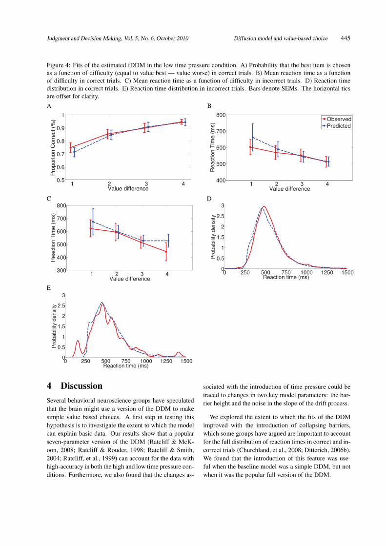
Figure 4: Fits of the estimated fDDM in the low time pressure condition. A) Probability that the best item is chosenas a function of difficulty (equal to value best — value worse) in correct trials. B) Mean reaction time as a functionof difficulty in correct trials. C) Mean reaction time as a function of difficulty in incorrect trials. D) Reaction timedistribution in correct trials. E) Reaction time distribution in incorrect trials. Bars denote SEMs. The horizontal ticsare offset for clarity.A B

1 2 3 40.5

0.6

0.7

0.8

0.9

1

Value difference

Pro

po

rtio

n C

orr

ect

(%)

1 2 3 4400

500

600

700

800

Value difference

Reaction Time (ms)

ObservedPredicted

C D

1 2 3 4300

400

500

600

700

800

Value difference

Re

actio

n T

ime

(m

s)

0 250 500 750 1000 1250 15000

0.5

1

1.5

2

2.5

3

Reaction time (ms)

Pro

ba

bili

ty d

en

sity

E

0 250 500 750 1000 1250 15000

0.5

1

1.5

2

2.5

3

Reaction time (ms)

Pro

babili

ty d

ensity

4 DiscussionSeveral behavioral neuroscience groups have speculatedthat the brain might use a version of the DDM to makesimple value based choices. A first step in testing thishypothesis is to investigate the extent to which the modelcan explain basic data. Our results show that a popularseven-parameter version of the DDM (Ratcliff & McK-oon, 2008; Ratcliff & Rouder, 1998; Ratcliff & Smith,2004; Ratcliff, et al., 1999) can account for the data withhigh-accuracy in both the high and low time pressure con-ditions. Furthermore, we also found that the changes as-

sociated with the introduction of time pressure could betraced to changes in two key model parameters: the bar-rier height and the noise in the slope of the drift process.

We explored the extent to which the fits of the DDMimproved with the introduction of collapsing barriers,which some groups have argued are important to accountfor the full distribution of reaction times in correct and in-correct trials (Churchland, et al., 2008; Ditterich, 2006b).We found that the introduction of this feature was use-ful when the baseline model was a simple DDM, but notwhen it was the popular full version of the DDM.


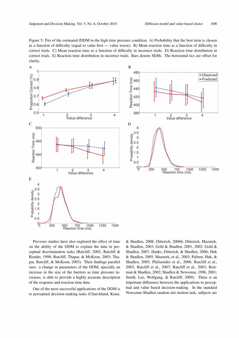
Figure 5: Fits of the estimated fDDM in the high time pressure condition. A) Probability that the best item is chosenas a function of difficulty (equal to value best — value worse). B) Mean reaction time as a function of difficulty incorrect trials. C) Mean reaction time as a function of difficulty in incorrect trials. D) Reaction time distribution incorrect trials. E) Reaction time distribution in incorrect trials. Bars denote SEMs. The horizontal tics are offset forclarity.

A B

1 2 3 40.5

0.6

0.7

0.8

0.9

1

Value difference

Pro

port

ion C

orr

ect (%

)

1 2 3 4380

400

420

440

460

480

Value difference

Re

actio

n T

ime

(m

s)

ObservedPredicted

C D

1 2 3 4350

400

450

500

Value difference

Reaction T

ime (

ms)

0 250 500 750 1000 1250 15000

0.5

1

1.5

2

2.5

3

3.5

4

Reaction time (ms)

Pro

babili

ty d

ensity

E

0 250 500 750 1000 1250 15000

0.5

1

1.5

2

2.5

3

3.5

4

Reaction time (ms)

Pro

babili

ty d

ensity

Previous studies have also explored the effect of timeon the ability of the DDM to explain the data in per-ceptual discrimination tasks (Ratcliff, 2002; Ratcliff &Rouder, 1998; Ratcliff, Thapar, & McKoon, 2003; Tha-par, Ratcliff, & McKoon, 2003). Their findings parallelours: a change in parameters of the DDM, specially anincrease in the size of the barriers as time pressure in-creases, is able to provide a highly accurate descriptionof the response and reaction time data.

One of the most successful applications of the DDM isto perceptual decision making tasks (Churchland, Kiani,

& Shadlen, 2008; Ditterich, 2006b; Ditterich, Mazurek,& Shadlen, 2003; Gold & Shadlen, 2001, 2002; Gold &Shadlen, 2007; Hanks, Ditterich, & Shadlen, 2006; Huk& Shadlen, 2005; Mazurek, et al., 2003; Palmer, Huk, &Shadlen, 2005; Philiastides et al., 2006; Ratcliff et al.,2003; Ratcliff et al., 2007; Ratcliff et al., 2003; Roit-man & Shadlen, 2002; Shadlen & Newsome, 1996, 2001;Smith, Lee, Wolfgang, & Ratcliff, 2009). There is animportant difference between the applications to percep-tual and value based decision-making. In the standardNewsome-Shadlen random dot motion task, subjects are


Figure 6: Estimated fitted drift rates in the sDDM byvalue distance. A) Low time pressure condition. B) Hightime pressure condition. Bars denote SEMs.

A

B

exposed to a stochastic stimulus that is assumed to gener-ate perceptual noise signals in area MT. Under appropri-ate assumptions, it can be shown that the drift-diffusionmodel implements an optimal decision-making processthat amounts to a sequential-likelihood ratio test (Bogacz,2007; Bogacz et al., 2006; Gold & Shadlen, 2001, 2002;Gold & Shadlen, 2007). In our model the stimuli are non-stochastic, in the sense that the image is non-changing.However, we hypothesize that in order to construct valuethe brain needs to integrate a series of noisy signals aboutthe value of the stimuli, in this case generated internally.In particular, we hypothesize that the brain assigns valueto the stimuli by sequentially and stochastically extract-ing features of the stimuli, retrieving the learnt valuesfor such features, and then integrating those values. Al-though the objective nature of the noise is quite differ-ent in both cases, the computational problem has similarproperties.

An important question for future research is how doesthe brain implement each of the features of the full DDMduring value based choices, which we have shown pro-vides a good quantitative description of the data.

References

Bogacz, R. (2007). Optimal decision-making theories:linking neurobiology with behaviour. Trends in Cogni-tive Science, 11, 118–125.

Bogacz, R., Brown, E., Moehlis, J., Holmes, P., & Cohen,J. D. (2006). The physics of optimal decision making:A formal analysis of models of performance in two-alternative forced choice tasks. Psychological Review,113, 700–765.

Brainard, D. H. (1997). The Psychophysics Toolbox.Spatial Vision, 10, 433–436.

Busemeyer, J. R., Jessup, R. K., Johnson, J. G., &Townsend, J. T. (2006). Building bridges between neu-ral models and complex decision making behaviour.Neural Netw, 19, 1047–1058.

Busemeyer, J. R., & Johnson, J. G. (2004). Computa-tional models of decision making. Cambridge, MA:Blackwell.

Decision-making with multiple alternatives, 11 Cong.Rec. 693–702 (2008).

Churchland, A. K., Kiani, R., & Shadlen, M. N. (2008).Decision-making with multiple alternatives. NatureNeuroscience, 11, 693–702.

Cisek, P., Puskas, G. A., & El-Murr, S. (2009). Decisionsin changing conditions: the urgency-gating model.Journal of Neuroscience, 29, 11560–11571.

Cornelissen, F. W., Peters, E. M., & Palmer, J. (2002).The Eyelink Toolbox: eye tracking with MATLAB andthe Psychophysics Toolbox. Behavior Research Meth-ods Instrumentats and Computers, 34, 613–617.

Ditterich, J. (2006a). Evidence for time-variant decisionmaking. European Journal of Neuroscience, 24, 3628–3641.

Ditterich, J. (2006b). Stochastic models of decisionsabout motion direction: behavior and physiology. Neu-ral Networks, 19, 981–1012.

Ditterich, J., Mazurek, M. E., & Shadlen, M. N. (2003).Microstimulation of visual cortex affects the speed ofperceptual decisions. Nature Neuroscience, 6, 891–898.

Fischer, B., & Weber, H. (1993). Express saccades andvisual attention. Behavioral and Brain Sciences, 16,553–610.

Gold, J. I., & Shadlen, M. N. (2001). Neural compu-tations that underlie decisions about sensory stimuli.Trends in Cognitive Sciences, 5, 10–16.

Gold, J. I., & Shadlen, M. N. (2002). Banburisms andthe brain: Decoding the relationship between sensorystimuli, decisions, and reward. Neuron, 36, 299–308.


Gold, J. I., & Shadlen, M. N. (2007). The neural basis ofdecision making. Annual Review of Neuroscience, 30,535–574.

Hanks, T. D., Ditterich, J., & Shadlen, M. N. (2006). Mi-crostimulation of macaque area LIP affects decision-making in a motion discrimination task. Nature Neu-roscience, 9, 682–689.

Hare, T., Camerer, C., Knoepfle, D., O’Doherty, J., &Rangel, A. (2009). Value computations in VMPFCduring charitable decision-making incorporate inputfrom regions involved in social cognition. Journal ofNeuroscience, 13, 583–590.

Hare, T., Camerer, C., & Rangel, A. (2009). Self-controlin decision-making involves modulation of the vMPFCvaluation system. Science, 324, 646–648.

Hare, T. A., O’Doherty, J., Camerer, C. F., Schultz, W.,& Rangel, A. (2008). Dissociating the role of the or-bitofrontal cortex and the striatum in the computationof goal values and prediction errors. Journal of Neuro-science, 28, 5623–5630.

Heekeren, H. R., Marrett, S., & Ungerleider, L. G.(2008). The neural systems that mediate human per-ceptual decision making. Nat Rev Neurosci.

Huk, A. C., & Shadlen, M. N. (2005). Neural activity inmacaque parietal cortex reflects temporal integration ofvisual motion signals during perceptual decision mak-ing. Journal of Neuroscience, 25, 10420–10436.

Link, S. W. (1992). The wave theory of difference andsimilarity. Cambridge: Psychology Press.

Mazurek, M. E., Roitman, J. D., Ditterich, J., & Shadlen,M. N. (2003). A role for neural integrators in per-ceptual decision making. Cerebral Cortex, 13, 1257–1269.

Padoa-Schioppa, C., & Assad, J. A. (2006). Neurons inthe orbitofrontal cortex encode economic value. Na-ture, 441, 223–226.

Palmer, J., Huk, A. C., & Shadlen, M. N. (2005). Theeffect of stimulus strength on the speed and accuracyof a perceptual decision. Journal of Vision, 5, 376–404.

Philiastides, M. G., Ratcliff, R., & Sajda, P. (2006). Neu-ral representation of task difficulty and decision mak-ing during perceptual categorization: a timing dia-gram. Journal of Neuroscience, 26, 8965–8975.

Rangel, A. (2008). The computation and comparison ofvalue in goal-directed choice. In P. W. Glimcher, C. F.Camerer, E. Fehr & R. A. Poldrack (Eds.), Neuroeco-nomics: Decision Making and the Brain. New York:Elsevier.

Rangel, A., Camerer, C., & Montague, P. R. (2008).A framework for studying the neurobiology of value-

based decision making. Nature Review of Neuro-science, 9, 545–556.

Rangel, A., & Hare, T. (2010). Neural computations as-sociated with goal-directed choice. Current Opinion inNeurobiology, 20, 262–270.

Ratcliff, R. (1978). A theory of memory retrieval. Psy-chological Review, 85, 59–108.

Ratcliff, R. (2002). A diffusion model account of reactiontime an accuracy in a brightness discrimination task:Fitting real data and failing to fit fake but plausibledata. Psychonomic Bulletin and Review, 9, 278–291.

Ratcliff, R., Cherian, A., & Segraves, M. (2003). Acomparison of macaque behavior and superior collicu-lus neuronal activity to predictions from models oftwo-choice decisions. Journal of Neurophysiology, 90,1392–1407.

Ratcliff, R., Hasegawa, Y. T., Hasegawa, R. P., Smith, P.L., & Segraves, M. A. (2007). Dual diffusion model forsingle-cell recording data from the superior colliculusin a brightness-discrimination task. Journal of Neuro-physiology, 97, 1756–1774.

Ratcliff, R., & Rounder, J. N. (2000). A diffusion modelaccount of masking in two-choice letter identification.Journal of Experimental Psychology: Human Percep-tion and Performance, 26, 127–140.

Ratcliff, R., & McKoon, G. (2008). The diffusion deci-sion model: Theory and data for two-choice decisiontasks. Neural Computation, 20, 873–922.

Ratcliff, R., Philiastides, M. G., & Sajda, P. (2009). Qual-ity of evidence for perceptual decision making is in-dexed by trial-to-trial variability of the EEG. Proceed-ings of the National Academy of Sciences, 106, 6539–6544.

Ratcliff, R., & Rouder, J. (1998). Modelling responsetimes for two-choice decisions. Pyschological Science,9, 347–356.

Ratcliff, R., & Smith, P. (2004). A comparison of se-quential sampling modles for two-choice reaction time.Psychological Review, 111, 333–367.

Ratcliff, R., Thapar, A., & McKoon, G. (2003). A diffu-sion model analysis of the effects of aging on bright-ness discrimination. Perception and Psychophysics,65, 523–535.

Ratcliff, R., Van Zandt, T., & McKoon, G. (1999). Con-nectionist and diffusion models of reaction time. Psy-chological Review, 106, 261–300.

Roitman, J. D., & Shadlen, M. N. (2002). Response ofneurons in the lateral intraparietal area during a com-bined visual discrimination reaction time task. Journalof Neuroscience, 22, 9475–9489.


Shadlen, M. N., & Newsome, W. T. (1996). Motion per-ception: seeing and deciding. Proceedings of the Na-tional Academy of Sciences, 93, 628–633.

Shadlen, M. N., & Newsome, W. T. (2001). Neural ba-sis of a perceptual decision in the parietal cortex (areaLIP) of the rhesus monkey. Journal of Neurophysiol-ogy, 86, 1916–1936.

Smith, P. L., Lee, Y. E., Wolfgang, B. J., & Ratcliff, R.(2009). Attention and the detection of masked radialfrequency patterns: Data and model. Vision Resesarch,49, 1363–1377.

Smith, P. L., & Ratcliff, R. (2004). Psychology and neu-robiology of simple decisions. Trends in Neuroscience,27, 161–168.

Thapar, A., Ratcliff, R., & McKoon, G. (2003). A dif-fusion model analysis of the effects of aging on letterdiscrimination. Psychology and Aging, 18, 415–429.

Tom, S. M., Fox, C. R., Trepel, C., & Poldrack, R. A.(2007). The neural basis of loss aversion in decision-making under risk. Science, 315, 515–518.

Tuerlinckx, F., Maris, E., Ratcliff, R., & De Boeck, P.(2001). A comparison of four methods for simulatingthe diffusion process. Behavior Research Methods, In-struments,& Computers, 33, 443–456.

Usher, M., & McClelland, J. (2001). The time course ofperceptual choice: the leaky, competing accumulatormodel. Psychological Review, 108, 550–592.

Usher, M., & McClelland, J. L. (2004). Loss aversionand inhibition in dynamical models of multialternativechoice. Psychological Review, 111, 757–769.

Vandekerckhove, J., & Tuerlinckx, F. (2008). Diffusionmodel analysis with MATLAB: A DMAT primer. Be-havioral Research Methods, 40, 61–72.

Wallis, J. D. (2007). Orbitofrontal cortex and its contri-bution to decision-making. Annual Review of Neuro-science, 30, 31–56.

Documents

The Drift Diffusion Model can account for the accuracy … and Decision Making, Vol. 5, No. 6, October 2010, pp. 437–449 The Drift Diffusion Model can account for the accuracy and