THE DRIVERS OF WAGE INEQUALITY ACROSS EUROPE: A …

1

THE DRIVERS OF WAGE INEQUALITY ACROSS EUROPE: A RECENTERED INFLUENCE FUNCTION REGRESSION APPROACH

JOÃO PEREIRA* and AURORA GALEGO&

*University of Évora, Department of Economics and CEFAGE-UE, Largo dos Colegiais, 2, 7000-803 Évora, Portugal, email: [email protected]; telefone/fax numbers:

00351266740894/00351266742494. Presenter.

& University of Évora, Department of Economics and CEFAGE-UE, Largo dos Colegiais, 2, 7000-803 Évora, Portugal, email: [email protected]

ABSTRACT

This study analyzes the impact of individual characteristics as well as occupation and industry on

male wage inequality in nine European countries. Unlike previous studies, we consider regression

models for five inequality measures and employ the recentered influence function regression

method proposed by Firpo et al. (2009) to test directly the influence of covariates on inequality.

We conclude that there is heterogeneity in the effects of covariates on inequality across countries

and throughout wage distribution. Heterogeneity among countries is more evident in education

and experience whereas occupation and industry characteristics as well as holding a supervisory

position reveal more similar effects. Our results are compatible with the skill biased technological

change, rapid rise in the integration of trade and financial markets as well as explanations related

to the increase of the remunerative package of top executives.

Keywords: inequality, inequality index, recentered influence function.

JEL Classification: C21; D31; J01.

mailto:[email protected]

2

I. Introduction

Inequality is an important topic in Economics and the issue has regained interest since the

eighties as several studies reported an increase in earnings inequality for Anglo-Saxon countries

(Lemieux, 2008). The trend towards greater inequality continued in the 1990s and 2000s,

spreading to other countries, particularly in Europe, although with differences (Lemieux, 2008,

Autor et al. 2008). In the case of Europe, recent studies have also documented great

heterogeneity concerning levels of earnings inequality among countries, suggesting that the most

unequal earnings can be observed in Portugal and Eastern European countries, while more

compressed earnings distributions are found in Scandinavian countries (Dreger et al., 2015 ; Van

Kerm and Pi Alperin, 2010).

An increasing number of studies have investigated the determinants of inequality as well as its

persistence. Most studies have considered individual countries, mainly the US and the UK (e.g.,

Card and DiNardo, 2002; Autor et al., 2008; Lemieux et al., 2009, Machin, 1997; Dickens and

Manning, 2004; Lindley and Machin, 2013), but others have analysed international differences in

inequality (e.g., Leuven et al., 2004; Martins and Pereira, 2004; Cholezas and Tsakloglou, 2009;

Simón, 2010; Budría and Pereira, 2011; Founier and Koske, 2012). This literature has put forward

two main explanations for increasing earnings inequality: the demand and supply of skilled

workers as a result of globalization and skill biased technological change and differences in

institutional settings.

In spite of the observed heterogeneity in inequality in Europe, not many studies using micro data

have provided comparative analysis about the determinants of wage inequality in European

countries. Moreover, typically, these studies have taken an indirect and partial approach. In fact,

3

some estimate wage equations and analyze the determinants of earnings at different points of the

distribution, therefore deducing (indirectly) the determinants of overall earnings inequality (e.g.,

Martins and Pereira, 2004; Budria and Pereira, 2011). Others, such as Simón (2010) or Chozelas

and Tsakloglou (2009), try to establish a direct relation between inequality and its determinants by

performing a decomposition of inequality indexes, but fail to analyze how this relationship

changes along the distribution.

This paper aims to increase knowledge about wage inequality in Europe, by investigating the

direct influence of several microeconomic characteristics (individual, occupational and industry)

on wage inequality levels within countries and how this influence changes along the wage

distribution. To perform this analysis, we estimate regression models for the determinants of

several inequality measures: the Gini index, the variance and the 90-10, 90-50 and 50-10 log

wage gaps. These regression models derive from the recentered influence function (RIF)

regression method proposed by Firpo et al. (2009). This methodology allows estimation of the

impact of small changes on covariates on the entire (unconditional) distribution of the dependent

variable (the inequality index). To the best of our knowledge, this is the first study presenting

regression models for log-wage gaps and testing directly inequality determinants on the set of

inequality measures presented. This analysis provides a better understanding about the direct

influence of microeconomic characteristics on wage inequality and how this influence changes

along the wage distribution.

We employ micro data on male workers from the European Union Statistics on Income and Living

Conditions (EU-SILC) for 2008 for a set of nine European countries (including both high inequality

and low inequality countries). Our findings show that there is heterogeneity as regards the

4

determinants of inequality across European countries, which is consistent with previous literature

(e.g., Simon,2010 or Chozelas and Tsakloglou, 2009).However, our results also show that the

impact of covariates is not the same for the various inequality measures. In fact, in addition to

previous studies, the results from the percentile log wage gaps regressions reveal that, in

general, the effect of covariates on inequality changes along the wage distribution and from one

country to another. This confirms the importance of using different inequality indexes as they

weigh different parts of the wage distribution differently1 (Melly, 2005).

In particular, adding previous literature, we conclude that heterogeneity across countries is more

evident regarding the effect of education and experience (seniority) on inequality. The

contribution of seniority to increased inequality is more apparent in poor countries, where there is

a higher share of low qualified workers. University education and especially secondary education

contribute to increased (decreased) inequality in countries where there is a lower (higher)

percentage of workers with these characteristics. Therefore, these results may justify investment

in education to reduce wage inequality directly, but also indirectly through lessening the

contribution of seniority components to pay and inequality.

The effects on inequality of the occupational structure and industry characteristics as well as

holding a supervisory position are more homogeneous among countries than in the case of

education and experience. The impact of these covariates on inequality varies mainly according

to industry and occupation. In general, the top categories of the occupational structure contribute

to increased inequality. However, there are coefficient differences among countries as regards

1The variance of logarithm of earnings is more sensitive to changes close to the bottom of the distribution, whereas

the Gini Index is more sensitive to changes around the Median (Cowell, 2000; Lambert, 2001)

5

the effect of these covariates. Therefore, there is heterogeneity in the magnitude of the impact,

but not regarding its direction.

In addition to previous literature, our results also show which industrial sectors contribute to

increased wage inequality, namely the highest and lowest paying industries. So inequality is also

a consequence of countries’ industrial specialization. Finally, working in the public sector or being

a native worker, in general, are not relevant factors in explaining wage inequality. The results

regarding education, industry and occupational structure are compatible with the skill biased

technological change, rapid rise in the integration of trade and financial markets as well as

explanations related to the increase in top executives’ remunerative packages.

The paper is organized as follows. The next section presents the methodology used in the paper.

Section 3 presents and analyzes the main characteristics of the data. Section 4 presents the

results and finally, Section 5 concludes.

2. Methodology

The method used in this paper is based on the recentered influence function (RIF) regression

approach developed by Firpo et al. (2009) and Firpo et al (2007). The RIF is defined as:

; ;RIF y v v F IF y v (1)

6

v F is a distributional statistic (ex: mean, variance, quantile, etc.) and ;IF y v is the

influence function (Hampel, 1974) associated with v F . The influence function represents the

influence of an individual observation on the distributional statistic. It can be shown that:

; ( ) 0IF y v dF y

(2)

This method is usually applied to a quantile (unconditional) regression problem, but can be easily

extended to other distributional statistics, such as the variance or the Gini index, provided that the

influence function of these distributional statistics is known. Hence, we have the following RIF

(Firpo et. al, 2007):

a) for quantiles:

;

y

y QRIF y Q Q

f Q

(3)

Where ( )yf Qis the marginal density of y at the point Q estimated by kernel methods; Q is the

sample quantile; ( )I y Q is an indicator function indicating whether the value of the outcome

variable is below Q .

The influence function for an inter-quantile range is given by the difference of the influence

functions at both quantiles (Andersen, 2008). Hence, for any q-quantile range given by:

1 , 0 0.5q q qQR y y where q

1

1

1

;q q

qq

q q

C if y y or y yf yRIF y QR QR

C if y y y

(4)

7

Where:

1

1 1

q q

C qf y f y

qQR is the sample quantile range (1 q qy y ) of the distribution of y (wages).

b) for the variance ( 2 ):

2 22( ; ) . ( )yRIF y y z dF z y u (5)

u : is the sample mean of y

c) for the Gini index:

2; 1 2( ) ;y yRIF y Gini B F y C y F (6)

Where

2

2

1

2

2 ( )

; 2 1 ( ) ;

Y y

Y y

B F R F

C y F y p y GL p y F

And 1

0

;Y YR F GL p F dp with Yp y F y and where ; yGL p F the generalized

Lorenz ordinate of YF is given by

1 ( )

;

F p

y yGL p F zdF z

.Further details can be found in

Firpo et al. (2007).

8

In this paper we estimate RIF regression models for the variance, Gini index and for the following

percentile log wage gaps: 90-10, 90-50 and 50-10. Hence, for each inequality measure an RIF is

estimated according to the procedures presented in equations (1) to (6). Then, in a second step,

as proposed by Firpo et al. (2009), we run an OLS regression of a new transformed dependent

variable – the RIF for the various distributional statistics – on the explanatory variables. The

standard errors of the estimated parameters are obtained by using the bootstrap procedure with

100 replications.

3. The data

We use data from The European Union Statistics on Income and Living Conditions (EU-SILC) for

the 2008 cross-sectional dataset. We considered this year to avoid our analysis being influenced

by the major impacts of the financial crisis and the fiscal adjustment programs in several

countries which occurred after 2008. EU-SILC is an annual survey from EUROSTAT, starting in

2004, which provides comparable data for the European Union on income, poverty, social

exclusion and living conditions. The survey also provides information on workers’ and other labor

market characteristics such as industry and occupation.

Our sample comprises full-time male employees aged 18 to 64 years old. Workers in agriculture

and fisheries, the self-employed, unpaid family workers and apprentices were excluded from the

sample. Finally, sample weights were applied in order to ensure sample representativeness.

Focusing on full-time male employees reduces the risks of comparability problems resulting from

different shares of part-time employment in different countries, differences in female labor market

9

participation and different discriminatory practices in relation to women. Moreover, as Atinson et

al. (2016) show, income from self-employment is not very reliable in EU-SILC when compared to

national accounts.

Hourly wages are computed dividing the gross amount received by employees in the main job,

before tax and social insurance contributions are deducted, by the number of hours of work.

Overtime pay, tips and commission as well as supplementary payments (13th and 14th month,

holiday payments) are included on a monthly proportional basis. This information is available only

for a limited group of countries, so we consider in our analysis the following countries: Austria

(AT), Greece (GR), Spain (ES), Hungary (HU), Ireland (IE), Italy (IT), Poland (PL), Portugal (PT)

and the United Kingdom (UK).

An alternative measure of labour income, such as previous year cash or near cash income

variable, would allow us to construct a measure of monthly earnings for a larger number of

countries. However, for most countries there is a non-negligible number of observations with zero

months of work and positive cash or near cash income.Furthermore, this variable relates to the

year previous to that in which the interview took place, while individual information about industry

and occupation is only available for the year of the interview.

As explanatory variables we use workers’ experience, two dummies for the highest educational

level achieved, nine occupational dummies (ISCO-88), nine dummies for industry affiliation

(NACE REV.1.1), a dummy for marital status, a dummy for supervisory position, a dummy for

workers born in the country of residence and another identifying public sector workers. There is

no direct information in the survey to distinguish between public and private sector workers.

10

Therefore, following previous studies, such as Giordano et al (2011), we consider as public sector

workers those working in one of the following sectors: public administration and defense,

compulsory social security, education, human health and social work activities.

Inequality measures computed with raw data are displayed in Table 1. The results confirm

previous studies’ conclusions about the existence of marked differences among European

countries with respect to their degree of wage inequality (OECD, 2011, Dreger et al, 2015). Yet

the results differ according to the inequality index. In fact, while Italy presents the lowest

inequality levels irrespective of the inequality index used, the highest levels of inequality vary

according to the inequality index: Hungary shows the highest value in the Gini index, whereas

Greece presents the maximum value for the variance. In addition, considering the percentile log

wage gap measures of inequality, Portugal shows the highest values taking as reference the 90-

10 log wage differential and the differential in the upper-tail of the wage distribution (90-50),

whereas the UK and Ireland present the highest values in the lower tail of the wage distribution.

This pattern is in accordance with previous evidence for these countries (Cardoso, 1998; Centeno

and Novo, 2014; Lemieux, 2008; OECD, 2011.)

[Table 1 around here]

Table 2 presents the descriptive statistics of the main explanatory variables used in the empirical

analysis. The UK and Ireland emerge as the countries with most workers with university

education as well as the highest percentage of workers in top occupations, particularly for

Legislators, senior officials and managers and Professionals. Likewise, these countries present

high shares of workers with supervisory responsibilities. Lower inequality countries, Austria and

11

Italy, are among those with a lower percentage of workers with a university degree. But unlike

Italy, Austria presents a high percentage of workers with secondary education. Moreover, both

countries show a low percentage of individuals working as Legislators, senior officials and

managers and Professionals, but the highest share of Technicians and associate professionals.

Eastern European countries (Hungary and Poland) present particularly high rates of workers with

secondary education and fewer workers performing supervisory tasks. One of the most unequal

countries, Portugal, shows the lowest percentages of workers with both secondary education and

a university degree and of workers in top occupations. In addition, Portugal also has the lowest

percentages of workers with supervisory responsibilities. Spain and Greece seem to be in an

intermediate position concerning both education and occupations.

Concerning the industrial structure and the percentage of workers in the public sector, again

Ireland and the UK reveal a similar pattern with the highest share of workers in the service sector

as well as of those working in the public sector. On the contrary, Portugal, Poland and Hungary

have the lowest share of workers in the services sector.

[Table 2 around here]

Regarding experience, Italy, Portugal and Greece show the most experienced labour force, while

UK workers are the least experienced among the countries in the sample. Finally, Austria has

most immigrants and in Eastern European countries almost all workers are native.

12

4. Results

The RIF estimations for the various distributional statistics and for the European countries

considered are presented in Tables 3 and 4. Considering first the effect of experience variables

(exper and exper2) on wage inequality, we may conclude this is not uniform in the European

countries considered, and even within each country the effects quite often change according to

the measure of inequality and/or range of the wage distribution. In fact, whereas in Hungary,

Italy, Poland, Portugal and Greece the experience variables contribute to increasing inequality for

most inequality measures, following the traditional profile of the experience effect on wages, in

Spain, Ireland and the UK, for most measures the effects of experience (and its square) on

inequality are not significant. In spite of this, there is some evidence of negative effects in the

lower tail of the wage distribution (50-10) in Spain and in the UK. Finally, in Austria, the effect of

experience on inequality is predominantly negative; however, the effects on the 90-10 and 90-50

wage gaps are not significant.

The t-ratios for the coefficient differences for each variable in relation to Italy2 , displayed in Table

5, show that experience variables (exper and exper2) are among the variables which present

more significant differences. In fact, returns to seniority are typically higher in Hungary, Poland

and Portugal and lower in Austria, Ireland and the UK, in relation to Italy. These results suggest

that returns to seniority have a more relevant role in determining inequality in poor countries than

in richer countries. Founier and Koske (2012) concluded that returns to experience are greater at

lower quantiles of the earnings distribution. Therefore, our results may reveal a higher share of

low-paid jobs in low-income countries (a composition effect).

2Italy presents the lowest levels of inequality in the sample.

13

The results regarding education are also quite heterogeneous among countries. Secondary

education is predominantly associated with lower inequality in the case of Austria, Spain and

Poland, while in Ireland, Italy and Portugal the opposite occurs. In the other countries, namely the

UK, Greece and Hungary, the effect of secondary education is in general not significant- the test

statistics in Table 5 confirm that these differences are statistically significant. Furthermore, the

effect of secondary education on inequality along the wage distribution is also not equal among

the countries. Indeed, while in Spain and Poland the narrowing effects in inequality appear in the

upper-tail of the wage distribution, in Austria this effect is stronger in the lower tail (50-10).

Likewise, a similar pattern occurs for the countries where secondary education contributes to

increasing wage inequality: in Ireland the positive effect is only significant in the 50-10 log wage

gap, whereas in Italy and Portugal it is only significant in the 90-50 log wage gap.

Referring to university education, this variable contributes to increasing wage inequality in the

cases of Hungary, Ireland (excluding the 90-10 and 90-50 wage gaps) and Italy, but contributes

to narrowing inequality in Austria. For other countries, the link between a university degree and

inequality is weaker, as few measures of inequality are positively or negatively associated with

this characteristic. In fact, in Spain and Poland, only the Gini index is negatively (and significantly)

associated with a university degree; in the UK only the variance is positively related; in Portugal a

university degree is positively related with inequality in the 90-10 and 50-10 log wage gaps; in

Greece, university education is positively related with the variance and the 90-10 wage gap.

Finally, as in the case of secondary education, the tests on the coefficient differences in relation

to Italy (Table 5) confirm that, apart from Ireland, these differences are in general significant.

Furthermore, in relation to Hungary, a country where a university degree contributes to increased

inequality, these tests show that the impact of this characteristic on inequality is higher than in

14

Italy. Therefore, as for secondary education, the effect of a university degree on inequality is quite

heterogeneous among countries.

We do not have direct evidence about the factors explaining these results, but the simple demand

and supply framework may provide some rationality. In fact, on the one hand, the generalized rise

in the supply of skilled workers over the last decades has contributed to decreasing wage

inequality (OECD, 2011). On the other hand, the increase in the demand for skilled workers as a

consequence of the skill biased technological change and of trade and financial integration, has

contributed to increasing skilled workers’ wages and therefore inequality, mainly for those with a

university degree (Lemieux, 2008; OECD, 2011).

The supply side explanation seems to be reasonable in the case of secondary education. In fact,

the increasing effect of secondary education on inequality seems to be more evident in countries

with the lowest percentages of workers with this characteristic, such as Ireland, Italy and

Portugal; the exception being Spain. On the other hand, cases of negative effects occur in

countries with higher percentages of individuals with secondary education, such as Hungary,

Austria and Poland.

In the case of a university degree, it is possible that demand side forces may have a stronger

role. Indeed, skill biased technological change and the integration of trade and financial markets

explanations favor the wages of highly skilled workers, namely those with a university degree

(OECD, 2011; Lemieux, 2008). Nevertheless, most situations of a positive association between

university education and inequality occur in countries with the lowest shares of university degrees

15

(IT, PT and HU) and cases of no significant influence or negative influence occur in countries with

high shares of individuals with this characteristic (ES, UK).Therefore, also in the case of

university-educated workers, these findings may result from differences in the supply of skilled

workers among countries. Ireland, which presents one of the highest percentages of individuals

with a university degree, seems to be a special case, as the huge number of foreign technological

firms located in this country may have contributed to reinforcing the demand for this kind of

worker and, therefore, their wages.

Obviously, it is not possible with this approach to disentangle demand and supply factors or to

understand how they influence the results in different countries. However, these heterogeneous

results as regards the effects of education on inequality may reflect different demand and supply

environments, in addition to existing institutional differences that may also contribute to this

heterogeneity.

Previous studies about the effects of education on inequality can also provide useful insights

intothis matter. For example, Martins and Pereira (2004) show that returns to education increase

along the wage distribution, contributing therefore to within group wage inequality. Budria and

Pereira (2011), in addition, found that the effect of education on inequality (within-group wage

inequality) is mainly driven by college education. They also found that for a certain number of

countries the returns to education decreased from the 1990s to the 2000s, which also reduced

the between component of inequality explained by education.Our inequality models measure the

contribution of the within and between components together. The results regarding the effect of a

university degree on wage inequality are compatible with this previous evidence of a positive

contribution of both components (within and between).

16

OECD (2011), in turn, presents evidence of negative effects of the increase in the work force’s

level of education on wage dispersion in a sample of 22 OECD countries from 1980 to

2008.Therefore, it is not surprising that by the end of the 2000s the link between education and

inequality had weakened and in some countries had become not significant or even negative.

Our results also suggest that investment in education, particularly in secondary education, may

be a route to reduce wage inequality. However, the race between the demand and supply of an

educated labor force (Tinbergen, 1975) may be more difficult in the case of university educated

workers. Hence, a higher effort of investment may be necessary in this level of education.

Furthermore, these investments in education may bring indirect benefits as more educated (and

more qualified) workers may also decrease inequality by reducing the role of the seniority

component on pay and hence on inequality.

[Table 3, around here]

Unlike the effect of experience and education, the results for occupational structure are more

homogenous among the countries. The category of Legislators, senior officials and managers, at

the top of the occupational structure, seems to increase inequality in almost all countries and for

the majority of the measures considered. The exceptions to this pattern are the UK and Ireland

where the effects are, in general, not significant. Moreover, in general, lower positions on the

occupational structure, corresponding to Professionals and Technicians and Associate

Professionals, also reveal a lower influence on wage inequality. In fact, in most cases, the

estimated coefficients decrease along the occupational structure, with the highest for Legislators,

17

senior officials and managers. In spite of this, there is some heterogeneity regarding the

magnitude of the estimated effect, as several significant differences are found among countries

(Table 5).

The positive effect of highly skilled occupations on wage inequality is in accordance with the

evidence provided by OECD (2011). However, adding to previous literature, our study also shows

that the effects of occupational structure on inequality are not equal along the wage distribution.

In Austria, Spain and Italy, the top category of the occupational structure contributes more to

wage inequality in the upper tail of the wage distribution. On the contrary, in Greece, Hungary,

Poland and Portugal, the effect on inequality is stronger in the lower tail (50-10 wage gap) and

higher than the estimated effect for Italy (Table 5).

In OECD (2011) this impact of highly skilled occupations is attributed to the rise in the integration

of trade and financial markets and to technological progress which raised the relative demand for

skilled workers. Piketty and Saez (2006) put forward other explanations, namely that

technological change made managerial skills more general (less enterprise specific), which

increased the competition for the best top executives, raising their relative wages. Another

explanation is related to pay-setting mechanisms for top executives which result in higher wages

for this group. In the same line, Lemieux et al. (2009) find that performance pay jobs increased

their share in the US wage distribution, which contributed to raising wage inequality, as inequality

is greater under this kind of pay scheme. More educated workers and those in highly paid

occupations are more likely to be involved in performance pay schemes. Therefore, this may be

another reason for highly skilled (and paid) occupations contributing positively to wage inequality.

Finally, offshoring activities are less likely to occur in some high paying professions such as

18

doctors and lawyers, which may be another factor contributing to increasing inequality in top

occupations.

Besides highly skilled occupations, workers with supervisory positions also seem to contribute to

a significant increase in wage inequality in most countries. Only in Austria, Ireland and the UK is

this result not confirmed, as the coefficient estimates are not significant. Moreover, most of the

remaining countries show several positive significant differences in relation to the Italian

estimates. Therefore, apart from Poland (90-50wage gap) this effect tends not to be lower than in

Italy, in Spain, Greece, Hungary and Portugal.

Our results also reveal that inter-industry wage differences are important in explaining wage

inequality in European economies, which agrees with previous evidence (Simon, 2010; Chozelas

and Tsakloglou, 2009). But as for occupations, the impact of industry sectors on inequality (Table

4) shows some degree of homogeneity among countries. Indeed, the test statistics in Table 5

confirm that most coefficient differences between each country and Italy are not significant. Unlike

previous studies, we also identify which industry sectors contribute to increased inequality in each

country and find that the impact on inequality in not the same along the wage distribution. Three

main industries show a significant and increasing influence on wage inequality: Financial

intermediation, Hotels and Restaurants and Transport, Storage and Communication. The first of

these industries presents more uniform results across countries and inequality measures. Indeed,

in five of the nine countries analyzed (ES, IT, PL, PT, UK) there are positive and significant

effects on inequality in almost all the measures considered, particularly in the upper-tail of the

wage distribution (90-50). Moreover, with the exception of Portugal, where most of the coefficient

differences are positive and significant, there are only a few significant differences for other

19

countries. Therefore, apart from countries’ compositional differences where the effect of this

industry on inequality is significant, financial intermediation seems to contribute more to inequality

within countries than to countries’ differences in inequality.

The Hotels and Restaurants industry has a significant influence on inequality in fewer countries,

namely in Spain and Poland, where the effects in the upper tail of the wage distribution are

greater than in the lower tail. Unsurprisingly, it is also in these two countries, but especially in

Poland, that we find significant coefficient differences in relation to Italy. Finally, the effects of

Transport, storage and communication industries are more evident in Spain and to a lesser extent

in Greece, but very few estimated differences in comparison to Italy are significant (ES: 90-50;

GR: Gini and variance). Studies on inter-industry wage differentials report that Financial

intermediation and the Transport, storage and communication industries are among the highest

paying industries in Europe, whereas Hotels and Restaurants is one of the lowest paying (Magda

et al. 2011; Caju et al. 2011). Therefore, the contribution of industry characteristics to wage

inequality is related to inter-industry wage differences.

Concerning the effect of being employed in the public sector on inequality, the results are not

significant for the majority of countries. The UK is the only exception, where inequality indexes

and public employment are, in general, negatively correlated. These findings are in accordance

with Grimshaw (2000), who found that in the case of the UK, the relatively centralized pay

arrangements in the public sector compared to those in the private sector contributed to

narrowing the increase in overall wage inequality from 1985 to 1995 (public and private sectors).

Budria (2010), in turn, in a sample of eight European countries3, found that the contribution of the

between component of education to wage inequality is similar in the public and private sectors,

3Finland, France, Germany, Italy, Norway, Portugal, Sweden and the UK.

20

but the within component is considerably lower in the public sector. Also, Fournier and Koske

(2012) found that higher shares of public employment are associated with a narrowing of the

earnings distribution. Therefore, negative or non-significant effects of public sector employment

on wage inequality agree with previous evidence that refers to the more centralized nature of pay

arrangements and more egalitarian concerns in the public sector.

[table 4, around here]

Finally, there is not much indication that the presence of non-native workers contributes to

increased inequality. In fact, only in the UK are native workers consistently associated with lower

levels of inequality, mainly in the upper part of the wage distribution (90-50). Furthermore, the

coefficients differences relatively to Italy are also in general significant For other countries, there

is some weak evidence of reducing inequality in Spain (Gini), Austria (90-50) and Italy (90-50)

and of increasing it in Hungary (50-10) and Greece (50-10); in Ireland, Poland and Portugal the

results are not statistically significant.

Our results are in line with previous empirical evidence for the US and other countries (Blau and

Kahn, 2012; Card, 2009) showing that, in general, the effects of immigration on wage inequality

are modest or inexistent. Yet our results indicate that the range of wage distribution and the

signal of the effects are not uniform across the countries considered.

5. Conclusions

In this study, we present and test a set of regression models for five commonly used inequality

measures (the Gini Index, the variance and the following log wage gaps: 90-10, 90-50 and 50-10)

using the recentered influence function regression approach. This regression methodology allows

21

direct testing of the influence of individual and other microeconomic characteristics on inequality

measures. To the best of our knowledge, this is the first work presenting regression models for

log-wage gaps and testing directly inequality determinants on the set of inequality measures

presented.

The analysis is carried out for male workers from nine European countries using data from the

European Union Statistics on Income and Living Conditions (EU SILC) for 2008. We focus on the

impact of individual characteristics as well as occupation and industry on wage inequality. Our

findings show that European countries differ significantly not only in the extent of wage inequality

but also in the relative importance of the factors shaping wage inequality. Furthermore, the impact

of covariates is not the same across inequality measures, particularly along the wage distribution.

Heterogeneity among countries is more evident in relation to education and experience.

Conversely, occupation, industry sectors and holding a supervisory position reveal more similar

effects. Working in the public sector and being a native worker are characteristics that, in general,

are not much relevant to wage inequality.

Regarding the effect of occupations, we conclude that highly paid occupations, particularly

Legislators, senior officials and managers, seem to significantly increase wage inequality in most

countries. Moreover, there are significant country differences regarding the magnitude of the

impact of occupations on inequality. Adding to previous literature, we also find that the impact of

occupations is not uniform along the wage distribution: there are countries where the influence is

higher in the upper tail, while in others the strongest effects are in the lower tail. Similarly, in

general, holding a supervisory position contributes to increased wage inequality.

22

Demand and supply conditions within each country may have a relevant role in explaining earlier

results regarding occupational structure and supervisory positions. However, our findings

concerning occupational structure are also compatible with more subtle explanations. Indeed,

higher relative wages for top executives may result from the increased demand for managerial

skills driven by technological progress or from the increase in the share of these workers involved

in performance pay schemes and other wage setting mechanisms. Also, some workers in this

category may be less likely to be involved in offshoring activities which may also contribute to

increasing their relative wages.

Inter-industry wage differentials within each country also contribute to increased wage inequality.

We complement previous evidence by concluding that highly paying industries such as

“Transport, storage and communication”, and especially “Financial intermediation”, contribute

significantly to increasing inequality as well as “Hotels and restaurants”, one of the low paying

industries. Moreover, we also find that the impacts on inequality in these sectors are stronger in

the upper tail of wage distribution than in the lower tail. However, apart from compositional

differences within each country, industry characteristics do not explain inequality differences

among countries, as very few significant coefficient differences among countries were found.

These results concerning the effect of industrial sectors also suggest that inequality reflects

countries’ industrial specialization.

Public sector workers’ effects on inequality are not entirely uniform across the set of European

countries considered, but our results reveal that for most countries this characteristic does not

contribute to increased wage inequality. This is in line with previous literature which indicates

lower levels of inequality in public sector workers. Also in accordance with previous evidence, we

23

find that the distinction between native and non-native workers does not add much to explaining

wage inequality. The exception is the case of the UK, where the native characteristic is

consistently associated with lower levels of wage inequality.

As for the effects of education and experience on inequality, countries show considerable

differences. Seniority payments (experience) seem to contribute to increased wage inequality in

countries where the work force is less qualified and where wages are lower, such as Hungary,

Poland, Italy, Portugal and Greece. In the remaining countries, typically experience does not

reveal significant effects on inequality, with the exception of Austria where experience contributes

to decreased inequality. Hence, a more qualified work force may be expected to mean lower

levels of wage inequality.

In relation to education, both secondary and university education variables have a positive impact

on inequality in some countries while in others the opposite occurs. In general, a university

degree and especially secondary education are predominantly associated with lower (higher)

inequality in countries with the highest (lowest) share of that type of worker. Furthermore, the

effects of education along the wage distribution are quite distinct among countries. These results

provide new evidence about the impact of education on inequality, as previous studies have

typically referred to an increasing contribution of education to wage inequality along the wage

distribution (Martins and Pereira, 2004, Budria and Pereira, 2011).

Our findings concerning education and experience may reflect different demand and supply

forces operating in each country. In particular, the results related to secondary education seem to

be closely linked to the supply of individuals with this characteristic. In the case of a university

degree, demand side factors may have a more relevant role in shaping our results. Indeed, skill

24

biased technological change and increased integration of trade and financial markets have

generated a rising demand for skilled workers, which favours the relative wages of this kind of

worker, contributing, therefore, to increased wage inequality in some countries. Hence, finding a

balanced race between the demand and supply of university educated workers may be more

difficult due to a higher relative demand for this kind of worker. However, the effort to promote

higher education may be worthwhile as this may also generate indirect effects through reducing

the role of seniority in inequality.

Finally, it should be noted that in addition to the different demand and supply conditions among

countries, it is also possible that countries’ heterogeneity as regard inequality and its

determinants is explained by differences in institutional settings, such as collective bargaining and

minimum wage regulations, which it was not possible to analyse in this work. Future research

should therefore investigate this aspect further.

Acknowledgements

The authors are pleased to acknowledge financial support from Fundação para a Ciência e a Tecnologia and FEDER/COMPETE (grant UID/ECO/04007/2013). This papers uses information from EU-SILC cross-sectional dataset for 2008 (rev.4) provided by Eurostat. Eurostat has no responsibility for the results and conclusions of this paper.

References

Anderson, R (2008) Modern Methods for Robust Regression. SAGE Publications: London.

Autor, A, Katz, L, Kearney, M. (2008) Trends in U.S. wage inequality: revising the revisionists.

The Review of Economics and Statistics 90, 300–323.

25

Berman E., Bound J., Griliches Z. (1994) Changes in the demand for skilled labor within US

manufacturing: evidence from the annual survey of manufactures. The Quarterly Journal of

Economics 109, 367-397.

Blau, F., Kahn, L. (2012), Immigration and the distribution of incomes, NBER Working paper

18515, National Bureau of Economic Research, Cambridge MA, USA.

Budría, S. (2010) Schooling and the distribution of wages in the European private and public

sectors. Applied Economics 42, 1045-1054.

Budría, S, Pereira, P (2011) Educational qualifications and wage inequality: evidence for Europe.

Revista de Economía Aplicada 56, 5-34.

Card, D. (2009), Immigration and inequality, American Economic Review 99, 1-21.

Card, D. , DiNardo, J. E. (2002)Skill-Biased Technological Change and Rising Wage Inequality:

Some Problems and Puzzles, Journal of Labor Economics 20, 733–783.

Cahuc, P, Zylberberg, A (2004) Labor Economics, The MIT Press: Cambridge.

Cardoso, A. (1998) Earnings inequality in Portugal: high and rising? Review of Income and

Wealth 44, 325-343.

Centeno, M, Novo, A (2014) When Supply Meets Demand: Wage Inequality in Portugal, IZA

Journal of European Labor Studies 3:23.

Chozelas, I.,Tsakloglou, P. (2009), “Earnings Inequality in Europe: Structure and Patterns of

Inter-Temporal Changes.” in Education and Inequality Across Europe (P. Dolton, R. Asplund and

E. Barth, eds) Cheltenham: Edward Elgar Publishing Ltd, 122-146.

26

Cowell F.A. (2000) “Measurement of inequality” (A.B. Atkinson and F. Bourguignon, eds)

Handbook of Income Inequality, Amsterdam: North Holland, Vol. I, 87-166.

Dickens, R., Manning, A. (2004) Has the national minimum wage reduced UK wage inequality?,

Journal of the Royal Statistical Society: Series A 167, 613-626

Dreger, C., López-Bazo,E., Ramos, R., Royuela, V., Suriñach, J. (2015) Wage and Income

Inequality in the European Union, European Parliament, Directorate-general for internal policies,

Committee on Employment and Social Affairs, available at :

http://www.europarl.europa.eu/studies.

Du Caju, P., Lamo, A., Poelhekke, S., Kátay, G., Nicolitsas, D. (2010) Inter-industry wage

differentials in EU countries: what do cross-country time varying data add to the picture?, Journal

of the European Economic Association 8, 478-486.

Firpo S., Fortin N., Lemieux T., (2007) Decomposing wage distributions using re-centered

influence function regressions, unpublished manuscript, University of British Columbia, June.

Firpo S., Fortin N., Lemieux T., (2009) Unconditional quantile regressions, Econometrica 77,

953-973.

Founier, J.M., Koske, I. (2012) The determinants of earnings Inequality: evidence from quantile

regressions. OECD Journal: Economic Studies 2012/1, 7-36.

Giordano R., Depalo D., Pereira M., Eugène B., Papapetrou E., Perez J., Reiss L. and Roter

M.(2011) The public sector pay gap in a selection of euro area countries, European Central Bank

WP Series, nº 1406

27

Grimshaw, D. (2000) Public Sector Employment, Wage Inequality and the Gender Pay Ratio in

the UK. International Review of Applied Economics 14, 427-448.

Hampel, F. R. (1974) The influence curve and its role in robust estimation. Journal of the

American Statistical Association 60, 383-393.

Lambert, P. (2001) The distribution and redistribution of income: A mathematical analysis,

3rd edition, Manchester University Press, Manchester.

Lemieux, T. (2008) The changing nature of wage inequality, Journal of Population Economics 21,

21-48.

Lemieux, T., Macleod WB, Parent, D.(2009) Performance pay and wage inequality. The Quarterly

Journal of Economics 124,1-49.

Lindley, J., Machin, S. (2013) Wage inequality in the Labour years, Oxford Review of Economic

Policy 29, 165–177

Leuven, E., Oosterbeek, H. van Ophem, H. (2004) Explaining international differences in male

skill wage differentials by differences in demand and supply of skill. The Economic Journal 114,

466–486.

Machin, S. (1997), ‘The Decline of Labour Market Institutions and the Rise in Wage Inequality in

Britain’, European Economic Review 41, 647–58.

Magda, I, Rycx, F, Tojerow, I (2011) Wage differentials across sectors in Europe: An east-west

comparison, Economics of Transition 19, 7649-769.

Martins, P, Pereira, P (2004) Does education reduce wage inequality? Quantile regression

evidence from 16 countries, Labour Economics 11, 355-371.

28

Melly, B. (2005) Decomposition of differences in distribution using quantile regression, Labour

Economics 12, 577–590.

Krueger, A. (1993) How computers have changed the wage structure: evidence from microdata,

1984–1989. Quarterly Journal of Economics, 108(1), 33–60.

Piketty, T, Saez, E (2006) The evolution of top incomes: a historical and international perspective,

American Economic Review 96, 200–205.

Simon, H (2010), International Differences in Wage Inequality: A New Glance with European

Matched Employer–Employee Data. British Journal of Industrial Relations 48, 310-346

OECD (2011), Divided we Stand: why Inequality Keeps Rising, OECD Publishing.

Tinbergen, J. (1975) Income Distribution: Analyses and Policies, North-Holland Publishing Co:

Amsterdam.

Van Kerm, P., Pi Alperin , M. N. (2010), Inequality, growth and mobility :the inter-temporal

distribution of income in European countries 2003-2007, Eurostat Methodologies and Working

Papers series, Population and social conditions.

1

TABLES

APPENDIX

Definition of variables

ln hourly wage The dependent variable is the logarithm of the hourly wage for employees. The

measure of wages corresponds to the gross amount received by employees in the

main job before tax and social insurance contributions were deducted. Overtime pay,

tips and commission as well as supplementary payments (13th and 14th month,

holiday payments) are included on a monthly proportional basis

Exper year of the survey- Year when highest level of education was attained

Exper2 exper2/100

Secondary education dummy variable; equals one if individual completed upper secondary education

(isced3); post-secondary non tertiary education included.

University degree dummy variable; equals one if individual has a university degree (isced5 or isced6)

Married dummy variable; equals one if individual is married or living in a consensual union.

Native dummy variable; equals one if individual has born in the country of residence.

Supervisory dummy variable; equals one if individual has a Supervisory responsibility.

Public sector dummy variable; equals one if individual if individual works in one of the following

sectors: public administration and defense, compulsory social security, education ,

human health and social work activities.

occupational dummies The estimations were carried out using dummies identifying occupations at one digit

level of aggregation according to the International Standard Classification of

Occupations (ISCO-88).

industry dummies The estimations were carried out using dummies at one digit level of aggregation

identifying the economic sector (NACE REV.1.1).

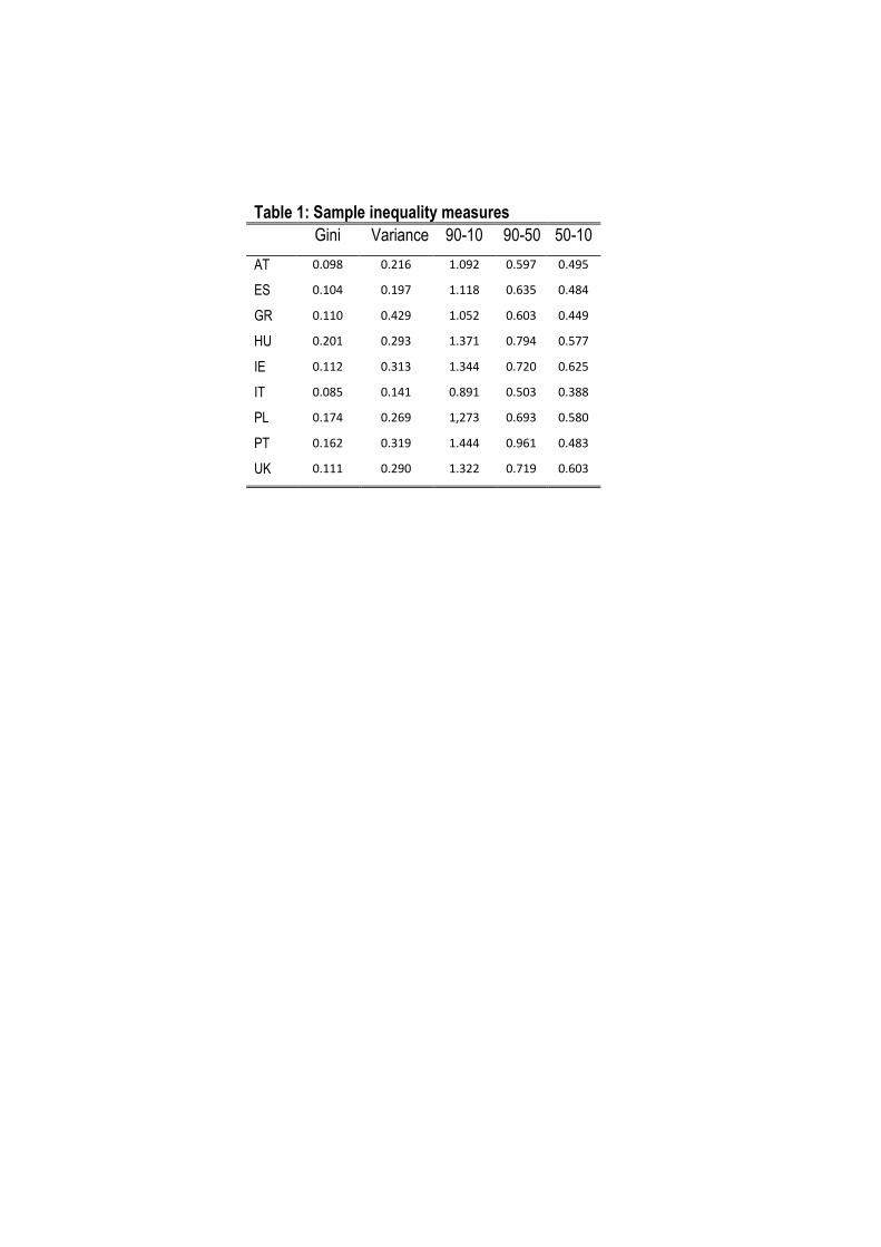
Table 1: Sample inequality measures

Gini Variance 90-10 90-50 50-10

AT 0.098 0.216 1.092 0.597 0.495

ES 0.104 0.197 1.118 0.635 0.484

GR 0.110 0.429 1.052 0.603 0.449

HU 0.201 0.293 1.371 0.794 0.577

IE 0.112 0.313 1.344 0.720 0.625

IT 0.085 0.141 0.891 0.503 0.388

PL 0.174 0.269 1,273 0.693 0.580

PT 0.162 0.319 1.444 0.961 0.483

UK 0.111 0.290 1.322 0.719 0.603

Table 2: Descriptive statistics for selected variables, 2008

AT ES GR HU IE IT PL PT UK

Experience 20.4

(12.3)

20.9

(12.7)

23.2

(13.2)

20.3

(12.0)

19.0

(15.0)

22.3

(12.6)

19.2

(13.0)

25.2

(17.2)

17.1

(13.2)

Secondary education 0.65

(0.48)

0.25

(0.43)

0.41

(0.49)

0.64

(0.48)

0.37

(0.48)

0.45

(0.50)

0.69

(0.46)

0.16

(0.37)

0.54

(0.50)

University degree 0.20

(0.40)

0.35

(0.47)

0.28

(0.45)

0.22

(0.41)

0.35

(0.48)

0.17

(0.38)

0.23

(0.42)

0.15

(0.35)

0.34

(0.47)

Supervisory 0.40

(0.49)

0.23

(0.42)

0.17

(0.37)

0.18

(0.38)

0.28

(0.45)

0.22

(0.42)

0.19

(0.39)

0.16

(0.36)

0.34

(0.47)

Legislators, 0.06 0.05 0.08 0.05 0.18 0.07 0.06 0.06 0.14

senior officials and managers

(0.24) (0.22) (0.27) (0.23) (0.38) (0.26) (0.23) (0.23) (0.35)

Professionals

0.10

(0.30)

0.13

(0.34)

0.16

(0.37)

0.13

(0.33)

0.19

(0.39)

0.11

(0.31)

0.15

(0.36)

0.09

(0.29)

0.15

(0.36)

Technicians and associate professionals

0.20

(0.40)

0.11

(0.32)

0.08

(0.27)

0.13

(0.34)

0.05

(0.22)

0.21

(0.40)

0.11

(0.32)

0.09

(0.29)

0.14

(0.34)

Clerks 0.13

(0.34)

0.13

(0.34)

0.11

(0.31)

0.09

(0.28)

0.12

(0.33)

0.12

(0.32)

0.07

(0.26)

0.09

(0.30)

0.14

(0.35)

Service workers and shop and market sales workers

0.14

(0.35)

0.16

(0.37)

0.14

(0.35)

0.15

(0.36)

0.19

(0.39)

0.11

(0.32)

0.12

(0.32)

0.16

(0.36)

0.16

(0.37)

Skilled agricultural and fishery workers

0.04

(0.20)

0.025

(0.16)

0.12

(0.32)

0.03

(0.17)

0.01

(0.07)

0.02

(0.14)

0.12

(0.32)

0.08

(0.26)

0.01

(0.10)

Craft and related trades workers

0.14

(0.34)

0.16

(0.36)

0.16

(0.37)

0.19

(0.39)

0.12

(0.32)

0.18

(0.38)

0.18

(0.38)

0.21

(0.41)

0.09

(0.29)

Plant and machine operators and assemblers

0.06

(0.24)

0.07

(0.26)

0.06

(0.24)

0.13

(0.34)

0.05

(0.32)

0.09

(0.29)

0.11

(0.31)

0.08

(0.28)

0.06

(0.25)

Public sector

0.22

(0.42)

0.22

(0.41)

0.22

(0.41)

0.22

(0.41)

0.28

(0.45)

0.22

(0.41)

0.19

(0.39)

0.20

(0.40)

0.29

(0.45)

Industrial sector 0.29

(0.45)

0.29

(0.45)

0.23

(0.42)

0.35

(0.48)

0.21

(0.41)

0.32

(0.47)

0.38

(0.49)

0.35

(0.48)

0.23

(0.42)

Services sector 0.71

(0.45)

0.71

(0.45)

0.77

(0.42)

0.65

(0.48)

0.79

(0.41)

0.68

(0.47)

0.62

(0.49)

0.65

(0.48)

0.77

(0.42)

Native 0.83

(0.38)

0.91

(0.29)

0.89

(0.31)

0.98

(0.14)

0.87

(0.34)

0.90

(0.30)

0.99

(0.06)

0.92

(0.27)

0.90

(0.31)

Note: standard errors are in parentheses.

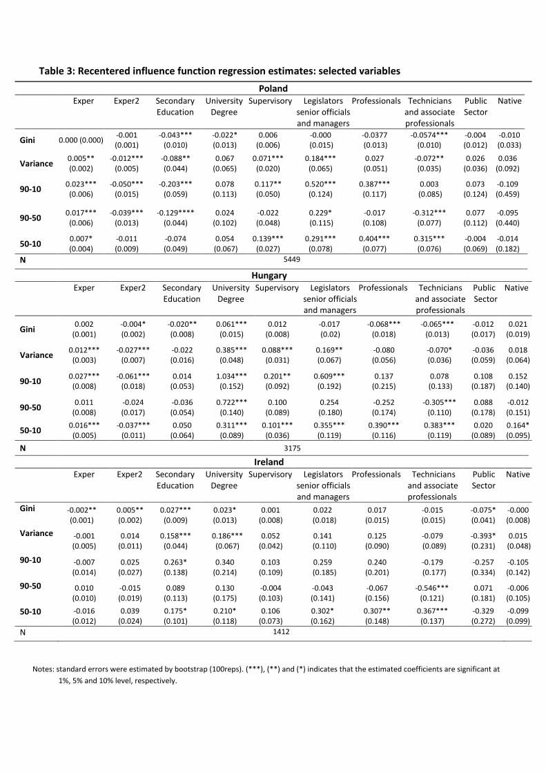
Table 3: Recentered influence function regression estimates: selected variables

Notes: standard errors were estimated by bootstrap (100reps). (***), (**) and (*) indicates that the estimated coefficients are significant at

1%, 5% and 10% level, respectively.

Poland

Exper Exper2 Secondary

Education

University

Degree

Supervisory Legislators

senior officials

and managers

Professionals Technicians

and associate

professionals

Public

Sector

Native

Gini 0.000 (0.000) -0.001

(0.001)

-0.043***

(0.010)

-0.022*

(0.013)

0.006

(0.006)

-0.000

(0.015)

-0.0377

(0.013)

-0.0574***

(0.010)

-0.004

(0.012)

-0.010

(0.033)

Variance 0.005**

(0.002)

-0.012***

(0.005)

-0.088**

(0.044)

0.067

(0.065)

0.071***

(0.020)

0.184***

(0.065)

0.027

(0.051)

-0.072**

(0.035)

0.026

(0.036)

0.036

(0.092)

90-10 0.023***

(0.006)

-0.050***

(0.015)

-0.203***

(0.059)

0.078

(0.113)

0.117**

(0.050)

0.520***

(0.124)

0.387***

(0.117)

0.003

(0.085)

0.073

(0.124)

-0.109

(0.459)

90-50 0.017***

(0.006)

-0.039***

(0.013)

-0.129****

(0.044)

0.024

(0.102)

-0.022

(0.048)

0.229*

(0.115)

-0.017

(0.108)

-0.312***

(0.077)

0.077

(0.112)

-0.095

(0.440)

50-10 0.007*

(0.004)

-0.011

(0.009)

-0.074

(0.049)

0.054

(0.067)

0.139***

(0.027)

0.291***

(0.078)

0.404***

(0.077)

0.315***

(0.076)

-0.004

(0.069)

-0.014

(0.182)

N 5449

Hungary


Education

University

Degree


senior officials

and managers


and associate

professionals

Public

Sector

Native

Gini 0.002

(0.001)

-0.004*

(0.002)

-0.020**

(0.008)

0.061***

(0.015)

0.012

(0.008)

-0.017

(0.02)

-0.068***

(0.018)

-0.065***

(0.013)

-0.012

(0.017)

0.021

(0.019)

Variance 0.012***

(0.003)

-0.027***

(0.007)

-0.022

(0.016)

0.385***

(0.048)

0.088***

(0.031)

0.169**

(0.067)

-0.080

(0.056)

-0.070*

(0.036)

-0.036

(0.059)

0.018

(0.064)

90-10 0.027***

(0.008)

-0.061***

(0.018)

0.014

(0.053)

1.034***

(0.152)

0.201**

(0.092)

0.609***

(0.192)

0.137

(0.215)

0.078

(0.133)

0.108

(0.187)

0.152

(0.140)

90-50 0.011

(0.008)

-0.024

(0.017)

-0.036

(0.054)

0.722***

(0.140)

0.100

(0.089)

0.254

(0.180)

-0.252

(0.174)

-0.305***

(0.110)

0.088

(0.178)

-0.012

(0.151)

50-10 0.016***

(0.005)

-0.037***

(0.011)

0.050

(0.064)

0.311***

(0.089)

0.101***

(0.036)

0.355***

(0.119)

0.390***

(0.116)

0.383***

(0.119)

0.020

(0.089)

0.164*

(0.095)

N 3175

Ireland


Education

University

Degree


senior officials

and managers


and associate

professionals

Public

Sector

Native

Gini -0.002**

(0.001)

0.005**

(0.002)

0.027***

(0.009)

0.023*

(0.013)

0.001

(0.008)

0.022

(0.018)

0.017

(0.015)

-0.015

(0.015)

-0.075*

(0.041)

-0.000

(0.008)

Variance -0.001

(0.005)

0.014

(0.011)

0.158***

(0.044)

0.186***

(0.067)

0.052

(0.042)

0.141

(0.110)

0.125

(0.090)

-0.079

(0.089)

-0.393*

(0.231)

0.015

(0.048)

90-10 -0.007

(0.014)

0.025

(0.027)

0.263*

(0.138)

0.340

(0.214)

0.103

(0.109)

0.259

(0.185)

0.240

(0.201)

-0.179

(0.177)

-0.257

(0.334)

-0.105

(0.142)

90-50 0.010

(0.010)

-0.015

(0.019)

0.089

(0.113)

0.130

(0.175)

-0.004

(0.103)

-0.043

(0.141)

-0.067

(0.156)

-0.546***

(0.121)

0.071

(0.181)

-0.006

(0.105)

50-10 -0.016

(0.012)

0.039

(0.024)

0.175*

(0.101)

0.210*

(0.118)

0.106

(0.073)

0.302*

(0.162)

0.307**

(0.148)

0.367***

(0.137)

-0.329

(0.272)

-0.099

(0.099)

N 1412

Table 3: Recentered influence function regression estimates: selected variables (cont.)

Notes: standard errors were estimated by bootstrap (100reps). (***), (**) and (*) indicates that the estimated coefficients are significant at

1%, 5% and 10% level, respectively

Portugal


Education

University

Degree


senior officials

and managers


and associate

professionals

Public

Sector

Native

Gini 0.002***

(0.001)

-0.004***

(0.001)

0.010

(0.009)

0.0179

(0.020)

0.022**

(0.010)

0.077*

(0.043)

0.093***

(0.026)

-0.002

(0.011)

0.028*

(0.017)

-0.007

(0.010)

Variance 0.017***

(0.004)

-0.028***

(0.008)

0.063

(0.048)

0.151

(0.111)

0.149***

(0.048)

0.515*

(0.265)

0.579***

(0.140)

0.086

(0.054)

0.167**

(0.079)

-0.052

(0.046)

90-10 0.031***

(0.013)

-0.054**

(0.023)

0.313**

(0.136)

0.534*

(0.309)

0.404***

(0.141)

1.014**

(0.415)

1.057***

(0.390)

0.369*

(0.175)

0.378

(0.243)

-0.204

(0.181)

90-50 0.026*

(0.014)

-0.046*

(0.024)

0.243*

(0.130)

0.339

(0.302)

0.261*

(0.137)

0.481

(0.430)

0.618

(0.384)

0.010

(0.160)

0.401

(0.261)

-0.160

(0.177)

50-10 0.005

(0.005)

-0.007

(0.009)

0.070

(0.063)

0.195**

(0.091)

0.143***

(0.050)

0.533***

(0.110)

0.439***

(0.121)

0.359***

(0.100)

-0.023

(0.143)

-0.044

(0.086)

N 1572

Spain


Education

University

Degree


senior officials

and managers


and associate

professionals

Public

Sector

Native

Gini -0.000

(0.000)

0.001

(0.001)

-0.013***

(0.003)

-0.007*

(0.004)

0.006**

(0.003)

0.058***

(0.012)

0.032***

(0.006)

-0.006

(0.005)

-0.002

(0.007)

-0.013**

(0.006)

Variance 0.001

(0.002)

-0.000

(0.004)

-0.032

(0.011)

0.005

(0.013)

0.042***

(0.012)

0.293***

(0.065)

0.174***

(0.025)

0.013

(0.022)

0.010

(0.025)

-0.039*

(0.022)

90-10 0.005

(0.005)

0.004

(0.009)

-0.128***

(0.043)

-0.025

(0.054)

0.113***

(0.041)

0.799***

(0.180)

0.563***

(0.092)

-0.004

(0.066)

0.109

(0.098)

-0.075

(0.068)

90-50 0.012**

(0.006)

-0.019*

(0.01)

-0.093**

(0.041)

0.006

(0.049)

0.022

(0.044)

0.565***

(0.167)

0.272***

(0.093)

-0.125**

(0.061)

0.085

(0.093)

-0.060

(0.054)

50-10 -0.007*

(0.004)

0.015**

(0.007)

-0.034

(0.037)

-0.031

(0.039)

0.090***

(0.030)

0.234***

(0.072)

0.291***

(0.057)

0.120**

(0.061)

0.024

(0.061)

-0.015

(0.058)

N 5440

Greece


Education

University

degree


senior officials

and managers


and associate

professionals

Public

Sector

Native

Gini 0.001

(0.001)

-0.001

(0.001)

-0.002

(0.005)

0.001

(0.006)

0.024***

(0.007)

0.036*

(0.021)

0.030***

(0.010)

0.008

(0.011)

-0.006

(0.011)

0.005

(0.006)

Variance 0.007***

(0.002)

-0.009**

(0.004)

0.010

(0.015)

0.049**

(0.025)

0.111***

(0.027)

0.165**

(0.083)

0.154***

(0.045)

0.096*

(0.049)

-0.012

(0.037)

0.018

(0.020)

90-10 0.019**

(0.009)

-0.025*

(0.017)

-0.005

(0.063)

0.151**

(0.063)

0.267***

(0.057)

0.533**

(0.100)

0.578**

(0.255)

0.165

(0.151)

-0.184

(0.164)

0.079

(0.058)

90-50 0.018**

(0.009)

-0.032**

(0.016)

-0.022

(0.050)

0.110

(0.10)

0.135

(0.097)

0.292

(0.232)

0.410***

(0.129)

0.011

(0.129)

-0.385**

(0.153)

-0.078

(0.049)

50-10 0.001

(0.005)

0.007

(0.011)

0.017

(0.044)

0.041

(0.062)

0.131***

(0.034)

0.240**

(0.111)

0.168**

(0.081)

0.154*

(0.086)

0.201**

(0.093)

0.157***

(0.051)

N 2018

Table 3: Recentered influence function regression estimates: selected variables (cont.)

Notes: standard errors were estimated by bootstrap (100reps). (***), (**) and (*) indicates that the estimated coefficients are significant at 1%,

5% and 10% level, respectively

Austria


Education

University

Degree


senior officials

and managers


Public

Sector

Native

Gini -0.003***

(0.001)

0.006 ***

(0.001)

-0.084***

(0.011)

-0.076

(0.105)

-0.005

(0.003)

0.051***

(0.14)

0.041***

(0.012)

0.02**

(0.009)

-0.023

(0.023)

-0.009

(0.007)

Variance -0.008***

(0.003)

0.019***

(0.007)

-0.303***

(0.046)

-0.241***

(0.051)

-0.006

(0.017)

0.265***

(0.069)

0.234***

(0.061)

0.113***

(0.040)

-0.095

(0.111)

-0.023

(0.04)

90-10 -0.014

(0.013)

0.042

(0.026)

-0.800***

(0.147)

-0.588***

(0.172)

0.056

(0.0556)

0.809***

(0.163)

0.644***

(0.150)

0.306***

(0.110)

-0.223

(0.187)

-0.133

(0.092)

90-50 0.004

(0.006)

0.002

(0.013)

-0.210***

(0.042)

-0.113

(0.077)

0.040

(0.040)

0.423***

(0.117)

0.306***

(0.116)

0.034

(0.059)

-0.116

(0.10)

-0.135***

(0.048)

50-10 -0.019*

(0.011)

0.040*

(0.021)

-0.589***

(0.147)

-0.475***

(0.165)

0.017

(0.044)

0.386***

(0.131)

0.338***

(0.110)

0.272***

(0.099)

-0.107

(0.161)

-0.107

(0.077)

N 2429

Italy


Education

University

degree


senior officials

and managers


Public

Sector

Native

Gini 0.000

(0.000)

0.000

(0.000)

0.004

(0.003)

0.033***

(0.005)

0.006**

(0.003)

0.062***

(0.013)

0.022***

(0.008)

-0.016

(0.005)

-0.005

(0.006)

-0.002

(0.004)

Variance 0.002**

(0.001)

-0.004*

(0.002)

0.021***

(0.007)

0.143***

(0.015)

0.035***

(0.007)

0.272

(0.055)

0.108

(0.028)

-0.042***

(0.015)

0.009

(0.020)

-0.002

(0.010)

90-10 0.008**

(0.004)

-0.015*

(0.009)

0.074**

(0.030)

0.434***

(0.075)

0.113***

(0.034)

0.664***

(0.159)

0.301***

(0.100)

-0.131**

(0.065)

-0.059

(0.080)

-0.045

(0.053)

90-50 0.014***

(0.003)

-0.026***

(0.006)

0.070***

(0.023)

0.350***

(0.068)

0.107***

(0.033)

0.666***

(0.125)

0.307***

(0.078)

-0.096**

(0.038)

-0.067

(0.063)

-0.080**

(0.034)

50-10 -0.007**

(0.003)

0.011

(0.007)

0.004

(0.026)

0.084**

(0.035)

0.006

(0.019)

-0.001

(0.081)

-0.006

(0.071)

-0.036

(0.062)

0.008

(0.052)

0.036

(0.042)

N 7085

United Kingdom


Education

University

degree


senior officials

and managers


and associate

professionals

Public

Sector

Native

Gini -0.002**

(0.001)

0.003**

(0.001)

0.004

(0.012)

0.012

(0.13)

-0.006

(0.004)

-0.014*

(0.008)

-0.035***

(0.008)

-0.030***

(0.009)

-0.026***

(0.009)

-0.017**

(0.007)

Variance -0.005*

(0.003)

0.009

(0.007)

0.051

(0.048)

0.124**

(0.051)

-0.012

(0.019)

0.041

(0.042)

-0.084*

(0.043)

-0.042

(0.062)

-0.166***

(0.044)

-0.091**

(0.041)

90-10 -0.005

(0.008)

0.000

(0.019)

-0.068

(0.237)

0.160

(0.243)

-0.022

(0.062)

0.044

(0.147)

-0.310**

(0.131)

-0.328**

(0.147)

-0.375***

(0.142)

-0.347***

(0.112)

90-50 0.004

(0.007)

-0.019

(0.016)

-0.031

(0.119)

0.076

(0.141)

-0.019

(0.058)

-0.065

(0.096)

-0.348***

(0.086)

-0.250***

(0.090)

-0.261***

(0.104)

-0.265***

(0.097)

50-10 -0.010*

(0.006)

0.019

(0.013)

-0.037

(0.253)

0.084

(0.259)

-0.003

(0.038)

0.109

(0.115)

0.038

(0.116)

-0.077

(0.129)

-0.114

(0.132)

-0.082

(0.070)

N 5449

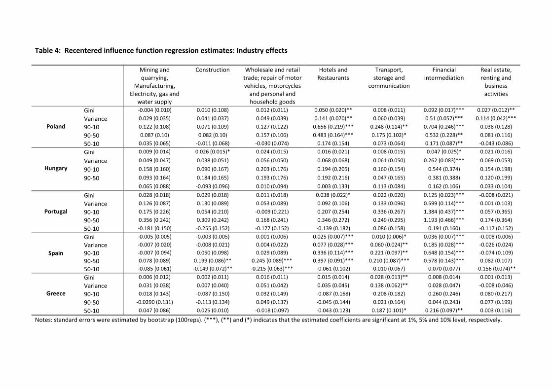
Table 4: Recentered influence function regression estimates: Industry effects

Mining and

quarrying,

Manufacturing,

Electricity, gas and

water supply

Construction

Wholesale and retail

trade; repair of motor

vehicles, motorcycles

and personal and

household goods

Hotels and

Restaurants

Transport,

storage and

communication

Financial

intermediation

Real estate,

renting and

business

activities

Poland

Gini -0.004 (0.010) 0.010 (0.108) 0.012 (0.011) 0.050 (0.020)** 0.008 (0.011) 0.092 (0.017)*** 0.027 (0.012)**

Variance 0.029 (0.035) 0.041 (0.037) 0.049 (0.039) 0.141 (0.070)** 0.060 (0.039) 0.51 (0.057)*** 0.114 (0.042)***

90-10 0.122 (0.108) 0.071 (0.109) 0.127 (0.122) 0.656 (0.219)*** 0.248 (0.114)** 0.704 (0.246)*** 0.038 (0.128)

90-50 0.087 (0.10) 0.082 (0.10) 0.157 (0.106) 0.483 (0.164)*** 0.175 (0.102)* 0.532 (0.228)** 0.081 (0.116)

50-10 0.035 (0.065) -0.011 (0.068) -0.030 (0.074) 0.174 (0.154) 0.073 (0.064) 0.171 (0.087)** -0.043 (0.086)

Hungary

Gini 0.009 (0.014) 0.026 (0.015)* 0.024 (0.015) 0.016 (0.021) 0.008 (0.015) 0.047 (0.025)* 0.021 (0.016)

Variance 0.049 (0.047) 0.038 (0.051) 0.056 (0.050) 0.068 (0.068) 0.061 (0.050) 0.262 (0.083)*** 0.069 (0.053)

90-10 0.158 (0.160) 0.090 (0.167) 0.203 (0.176) 0.194 (0.205) 0.160 (0.154) 0.544 (0.374) 0.154 (0.198)

90-50 0.093 (0.164) 0.184 (0.165) 0.193 (0.176) 0.192 (0.216) 0.047 (0.165) 0.381 (0.388) 0.120 (0.199)

0.065 (0.088) -0.093 (0.096) 0.010 (0.094) 0.003 (0.133) 0.113 (0.084) 0.162 (0.106) 0.033 (0.104)

Portugal

Gini 0.028 (0.018) 0.029 (0.018) 0.011 (0.018) 0.038 (0.022)* 0.022 (0.020) 0.125 (0.023)*** -0.008 (0.021)

Variance 0.126 (0.087) 0.130 (0.089) 0.053 (0.089) 0.092 (0.106) 0.133 (0.096) 0.599 (0.114)*** 0.001 (0.103)

90-10 0.175 (0.226) 0.054 (0.210) -0.009 (0.221) 0.207 (0.254) 0.336 (0.267) 1.384 (0.437)*** 0.057 (0.365)

90-50 0.356 (0.242) 0.309 (0.242) 0.168 (0.241) 0.346 (0.272) 0.249 (0.295) 1.193 (0.466)*** 0.174 (0.364)

50-10 -0.181 (0.150) -0.255 (0.152) -0.177 (0.152) -0.139 (0.182) 0.086 (0.158) 0.191 (0.160) -0.117 (0.152)

Spain

Gini -0.005 (0.005) -0.003 (0.005) 0.001 (0.006) 0.025 (0.007)*** 0.010 (0.006)* 0.036 (0.007)*** -0.008 (0.006)

Variance -0.007 (0.020) -0.008 (0.021) 0.004 (0.022) 0.077 (0.028)*** 0.060 (0.024)** 0.185 (0.028)*** -0.026 (0.024)

90-10 -0.007 (0.094) 0.050 (0.098) 0.029 (0.089) 0.336 (0.114)*** 0.221 (0.097)** 0.648 (0.154)*** -0.074 (0.109)

90-50 0.078 (0.089) 0.199 (0.086)** 0.245 (0.089)*** 0.397 (0.091)*** 0.210 (0.087)*** 0.578 (0.143)*** 0.082 (0.107)

50-10 -0.085 (0.061) -0.149 (0.072)** -0.215 (0.063)*** -0.061 (0.102) 0.010 (0.067) 0.070 (0.077) -0.156 (0.074)**

Greece

Gini 0.006 (0.012) 0.002 (0.011) 0.016 (0.011) 0.015 (0.014) 0.028 (0.013)** 0.008 (0.014) 0.001 (0.013)

Variance 0.031 (0.038) 0.007 (0.040) 0.051 (0.042) 0.035 (0.045) 0.138 (0.062)** 0.028 (0.047) -0.008 (0.046)

90-10 0.018 (0.143) -0.087 (0.150) 0.032 (0.149) -0.087 (0.168) 0.208 (0.182) 0.260 (0.246) 0.080 (0.217)

90-50 -0.0290 (0.131) -0.113 (0.134) 0.049 (0.137) -0.045 (0.144) 0.021 (0.164) 0.044 (0.243) 0.077 (0.199)

50-10 0.047 (0.086) 0.025 (0.010) -0.018 (0.097) -0.043 (0.123) 0.187 (0.101)* 0.216 (0.097)** 0.003 (0.116)

Notes: standard errors were estimated by bootstrap (100reps). (***), (**) and (*) indicates that the estimated coefficients are significant at 1%, 5% and 10% level, respectively.

Table 4: Recentered influence function regression estimates: Industry effects (cont.)

Mining and

quarrying,

Manufacturing,

Electricity, gas and

water supply

Construction Wholesale and retail

trade; repair of motor

vehicles, motorcycles

and personal and

household goods

Hotels and

Restaurants

Transport,

storage and

communication

Financial

intermediation

Real estate, renting

and business

activities

Gini -0.066 (0.015)*** -0.073 (0.016)*** -0.071 (0.015)*** -0.071 (0.019)*** -0.077 (0.017)*** -0.039 (0.017)** -0.067 (0.016)***

Ireland Variance -0.360 (0.092)*** -0.409 (0.095)*** -0.440 (0.091)*** -0.465 (0.115)*** -0.455 (0.103)*** -0.199 (0.106)* -0.417 (0.096)***

90-10 -0.413 (0.329) -0.420 (0.321) -0.396 (0.315) -0.213 (0.428) -0.417 (0.354) -0.097 (0.411) -0.391 (0.379)

90-50 -0.092 (0.188) -0.144 (0.175) 0.133 (0.182) 0.261 (0.177) -0.236 (0.186) 0.353 (0.265) 0.151 (0.177)

50-10 -0.322 (0.276) -0.276 (0.264) -0.529 (0.277)* -0.475 (0.365) -0.181 (0.293) -0.450 (0.296) -0.542 (0.326)

Austria

Gini -0.029 (0.010)*** -0.036 (0.011)*** -0.013 (0.011) 0.017 (0.014) -0.021 (0.012)** -0.013 (0.013) -0.027 (0.011)**

Variance -0.122 (0.049)** -0.150 (0.053)*** -0.066 (0.051) 0.016 (0.068 -0.072 (0.056) -0.053 (0.065) -0.124 (0.055)**

90-10 -0.212 (0.182) -0.239 (0.202) -0.068 (0.189) 0.488 (263)* -0.225 (0.190) 0.178 (0.225) -0.089 (0.212)

90-50 -0.116 (0.095) -0.087 (0.104) -0.005 (0.104) 0.090 (0.108) -0.101 (0.108) 0.218 (0.173) -0.034 (0.110)

50-10 -0.095 (0.168) -0.152 (0.196) -0.063 (0.169) 0.397 (0.239)* -0.124 (0.169) -0.040 (0.183) -0.056 (0.181)

Italy

Gini -0.007 (0.004)* 0.004 (0.004) 0.008 (0.004)* 0.015 (0.006)** -0.003 (0.005) 0.029 (0.006)*** 0.000 (0.005)

Variance -0.012 (0.014) 0.015 (0.016) 0.025 (0.015)* 0.038 (0.022)* 0.000 (0.016) 0.112 (0.020)*** 0.000 (0.018)

90-10 -0.033 (0.076) 0.093 (0.084) 0.076 (0.074) 0.138 (0.116) 0.032 (0.073) 0.363 (0.139)*** -0.060 (0.089)

90-50 0.003 (0.055) 0.051 (0.058) 0.068 (0.054) 0.034 (0.069) -0.047 (0.060) 0.219 (0.128)* -0.033 (0.071)

50-10 -0.035 (0.053) 0.041 (0.066) 0.008 (0.057) 0.104 (0.089) 0.079 (0.051) 0.144 (0.054)*** -0.027 (0.059)

UK

Gini -0.015 (0.010) -0.008 (0.011) 0.008 (0.010) 0.046 (0.016)*** -0.016 (0.011) 0.036 (0.011)*** 0.006 (0.010)

Variance -0.026 (0.056) 0.027 (0.061) 0.070 (0.060) 0.227 (0.094)** -0.014 (0.062) 0.289 (0.067)*** 0.093 (0.058)

90-10 -0.230 (0.141) -0.228 (0.145) -0.080 (0.157) 0.372 (0.305) -0.221 (0.169) 0.599 (0.235)*** 0.101 (0.170)

90-50 -0.141 (0.104) -0.122 (0.101) -0.002 (0.103) 0.095 (0.200) 0.009 (0.125) 0.604 (0.187)*** 0.021 (0.127)

50-10 -0.089 (0.118) -0.106 (0.129) -0.078 (0.136) 0.277 (0.233) -0.231 (0.126)* -0.005 (0.149) 0.080 (0.134)

Notes: standard errors were estimated by bootstrap (100reps). (***), (**) and (*) indicates that the estimated coefficients are significant at 1%, 5% and 10% level, respectively.

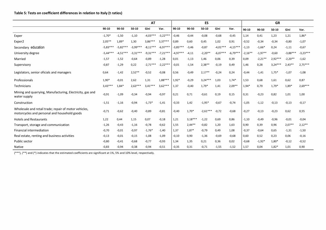
Table 5: Tests on coefficient differences in relation to Italy (t ratios)

AT ES GR

90-10 90-50 50-10 Gini Var. 90-10 90-50 50-10 Gini Var. 90-10 90-50 50-10 Gini Var.

Exper -1,70* -1,50 -1,10 -4,03*** -3,22*** -0,46 -0,44 -0,08 -0,68 -0,45 1,14 0,41 1,23 1,21 1,86*

Exper2 2,05** 1,89* 1,30 3,86*** 3,37*** 0,89 0,60 0,45 1,02 0,91 -0,52 -0,34 -0,34 -0,80 -1,07

Secondary education -5,83*** -5,82*** -3,99*** -8,11*** -6,97*** -3,85*** -3,46 -0,87 -4,01*** -4,15*** -1,13 -1,66* 0,24 -1,11 -0,67

University degree -5,44*** -4,51*** -3,31*** -9,31*** -7,21*** -4,97*** -4,11 -2,20** -6,07*** -6,79*** -2,16** -1,97** -0,60 -3,88*** -3,23***

Married -1,57 -1,52 -0,64 -0,89 -1,28 0,01 -1,13 1,46 0,06 0,39 0,09 -2,21** 2,92*** -2,20** -1,62

Supervisory -0,87 -1,29 0,22 -2,71*** -2,22*** -0,01 -1,54 2,38** -0,19 0,49 1,46 0,28 3,24*** 2,43** 2,75***

Legislators, senior oficials and managers 0,64 -1,42 2,52** -0,52 -0,08 0,56 -0,49 2,17** -0,24 0,24 -0,44 -1,41 1,75* -1,07 -1,08

Professionals 1,90* -0,01 2,62 1,31 1,88*** 1,92* -0,29 3,24*** 1,03 1,74* 1,53 0,68 1,61 0,62 0,87

Technicians 3,43*** 1,84* 2,63*** 3,41*** 3,62*** 1,37 -0,40 1,79* 1,41 2,09** 1,94* 0,79 1,79* 1,89* 2,69***

Mining and quarrying, Manufacturing, Electricity, gas and water supply

-0,91 -1,09 -0,34 -0,94 -0,97 0,21 0,71 -0,61 0,19 0,15 0,31 -0,23 0,82 1,01 1,00

Construction -1,51 -1,16 -0,94 -1,73* -1,41 -0,33 1,42 -1,95* -0,67 -0,74 -1,05 -1,12 -0,13 -0,13 -0,17

Wholesale and retail trade; repair of motor vehicles, motorcycles and personal and household goods

-0,71 -0,62 -0,40 -0,89 -0,81 -0,40 1,70* -2,61*** -0,72 -0,68 -0,27 -0,13 -0,23 0,62 0,55

Hotels and Restaurants 1,22 0,44 1,15 0,07 -0,18 1,21 3,18*** -1,22 0,69 0,86 -1,10 -0,49 -0,96 -0,01 -0,04

Transport, storage and communication -1,26 -0,43 -1,16 -0,78 -0,62 1,55 2,44** -0,82 1,20 1,63 0,90 0,39 0,96 2,07** 2,12**

Financial intermediation -0,70 -0,01 -0,97 -1,76* -1,40 1,37 1,87* -0,79 0,49 1,08 -0,37 -0,64 0,65 -1,31 -1,50

Real estate, renting and business activities -0,13 -0,01 -0,15 -1,08 -1,09 -0,10 0,90 -1,36 -0,69 -0,68 0,60 0,52 0,23 0,06 -0,16

Public sector -0,80 -0,41 -0,68 -0,77 -0,93 1,34 1,35 0,21 0,36 0,02 -0,68 -1,92* 1,80* -0,12 -0,52

Native -0,83 -0,94 -0,38 -0,94 -0,51 -0,35 0,31 -0,71 -1,55 -1,52 1,57 0,04 1,82* 1,01 0,90

(***), (**) and (*) indicates that the estimated coefficients are significant at 1%, 5% and 10% level, respectively.

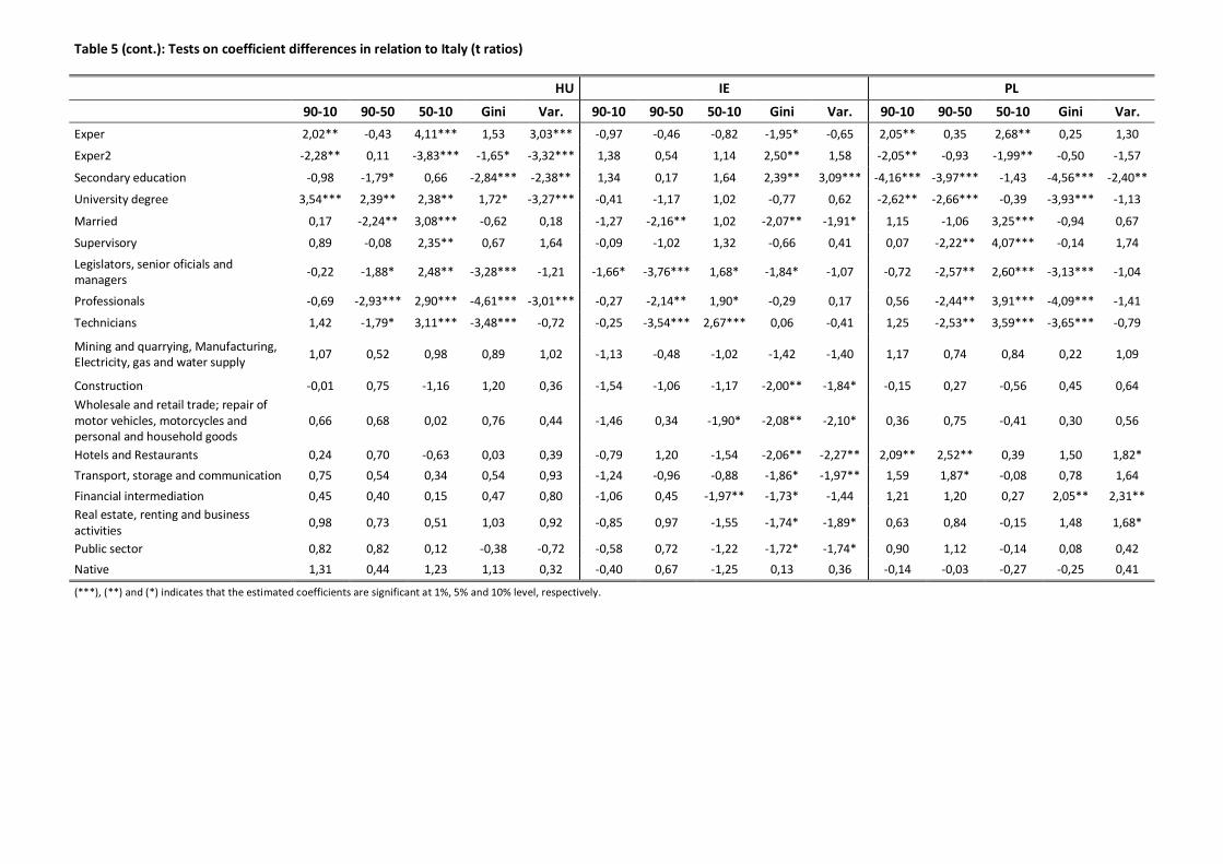
Table 5 (cont.): Tests on coefficient differences in relation to Italy (t ratios)

HU IE PL

90-10 90-50 50-10 Gini Var. 90-10 90-50 50-10 Gini Var. 90-10 90-50 50-10 Gini Var.

Exper 2,02** -0,43 4,11*** 1,53 3,03*** -0,97 -0,46 -0,82 -1,95* -0,65 2,05** 0,35 2,68** 0,25 1,30

Exper2 -2,28** 0,11 -3,83*** -1,65* -3,32*** 1,38 0,54 1,14 2,50** 1,58 -2,05** -0,93 -1,99** -0,50 -1,57

Secondary education -0,98 -1,79* 0,66 -2,84*** -2,38** 1,34 0,17 1,64 2,39** 3,09*** -4,16*** -3,97*** -1,43 -4,56*** -2,40**

University degree 3,54*** 2,39** 2,38** 1,72* -3,27*** -0,41 -1,17 1,02 -0,77 0,62 -2,62** -2,66*** -0,39 -3,93*** -1,13

Married 0,17 -2,24** 3,08*** -0,62 0,18 -1,27 -2,16** 1,02 -2,07** -1,91* 1,15 -1,06 3,25*** -0,94 0,67

Supervisory 0,89 -0,08 2,35** 0,67 1,64 -0,09 -1,02 1,32 -0,66 0,41 0,07 -2,22** 4,07*** -0,14 1,74

Legislators, senior oficials and managers

-0,22 -1,88* 2,48** -3,28*** -1,21 -1,66* -3,76*** 1,68* -1,84* -1,07 -0,72 -2,57** 2,60*** -3,13*** -1,04

Professionals -0,69 -2,93*** 2,90*** -4,61*** -3,01*** -0,27 -2,14** 1,90* -0,29 0,17 0,56 -2,44** 3,91*** -4,09*** -1,41

Technicians 1,42 -1,79* 3,11*** -3,48*** -0,72 -0,25 -3,54*** 2,67*** 0,06 -0,41 1,25 -2,53** 3,59*** -3,65*** -0,79


1,07 0,52 0,98 0,89 1,02 -1,13 -0,48 -1,02 -1,42 -1,40 1,17 0,74 0,84 0,22 1,09

Construction -0,01 0,75 -1,16 1,20 0,36 -1,54 -1,06 -1,17 -2,00** -1,84* -0,15 0,27 -0,56 0,45 0,64


0,66 0,68 0,02 0,76 0,44 -1,46 0,34 -1,90* -2,08** -2,10* 0,36 0,75 -0,41 0,30 0,56

Hotels and Restaurants 0,24 0,70 -0,63 0,03 0,39 -0,79 1,20 -1,54 -2,06** -2,27** 2,09** 2,52** 0,39 1,50 1,82*

Transport, storage and communication 0,75 0,54 0,34 0,54 0,93 -1,24 -0,96 -0,88 -1,86* -1,97** 1,59 1,87* -0,08 0,78 1,64

Financial intermediation 0,45 0,40 0,15 0,47 0,80 -1,06 0,45 -1,97** -1,73* -1,44 1,21 1,20 0,27 2,05** 2,31**

Real estate, renting and business activities

0,98 0,73 0,51 1,03 0,92 -0,85 0,97 -1,55 -1,74* -1,89* 0,63 0,84 -0,15 1,48 1,68*

Public sector 0,82 0,82 0,12 -0,38 -0,72 -0,58 0,72 -1,22 -1,72* -1,74* 0,90 1,12 -0,14 0,08 0,42

Native 1,31 0,44 1,23 1,13 0,32 -0,40 0,67 -1,25 0,13 0,36 -0,14 -0,03 -0,27 -0,25 0,41


Table 5 (cont.): Tests on coefficient differences in relation to Italy (t ratios)

PT UK

90-10 90-50 50-10 Gini Var. 90-10 90-50 50-10 Gini Var.

Exper 1,68* 0,86 1,98** 2,94*** 3,11*** -1,47 -1,31 -0,52 -2,74*** -2,36**

Exper2 -1,59 -0,84 -1,68* -2,59** -2,94*** 0,72 0,40 0,54 2,31** 1,78*

Secondary education 1,71* 1,31 0,95 0,80 0,88 -0,60 -0,83 -0,16 -0,02 0,62

University degree 0,32 -0,04 1,14 -0,74 0,07 -1,08 -1,75* 0,00 -1,53 -0,36

Married 0,68 0,27 0,76 -0,97 -0,25 0,68 0,48 0,37 -0,30 -0,27

Supervisory 2,01** 1,09 2,55** 1,53 2,37** -1,92* -1,89* -0,21 -2,60*** -2,27**

Legislators, senior oficials and managers 0,79 -0,41 3,91*** 0,33 0,90 -2,87*** -4,64*** 0,78 -4,94*** -3,37***

Professionals 1,88* 0,79 3,16*** 2,59** 3,29*** -3,71*** -5,64*** 0,32 -5,12*** -3,73***

Technicians 2,68*** 0,65 3,37*** 1,04 2,27** -1,22 -1,58 -0,29 -1,26 0,01


0,87 1,43 -0,92 1,85* 1,67* -1,23 -1,22 -0,42 -0,77 -0,31

Construction -0,17 1,04 -1,79* 1,20 1,25 -1,91* -1,48 -1,02 -0,80 0,18


-0,36 0,40 -1,13 0,12 0,32 -0,90 -0,60 -0,58 -0,04 0,73

Hotels and Restaurants 0,25 1,11 -1,20 0,74 0,57 0,72 0,29 0,69 1,22 1,65*

Transport, storage and communication 1,10 0,98 0,05 1,13 1,33 -1,38 0,41 -2,28** -1,24 -0,28

Financial intermediation 2,23** 2,02** 0,28 3,49*** 3,49*** 0,86 1,70* -0,95 0,44 2,06**

Real estate, renting and business activities 0,31 0,56 -0,55 -0,30 0,00 0,84 0,37 0,73 0,54 1,75*

Public Sector 1,71* 1,74* -0,20 1,87* 1,94* -1,94* -1,59 -0,85 -1,92* -1,67*

Native -0,84 -0,44 -0,83 -0,47 -1,07 -2,44** -1,78* -1,44 -1,88* -2,08**


Documents

THE DRIVERS OF WAGE INEQUALITY ACROSS EUROPE: A …