Embed Size (px)
Citation preview

The Effect of Police Response Timeon Crime Detection∗
Jordi Blanes i Vidal† and Tom Kirchmaier‡
October 7, 2015
Abstract
Police agencies devote vast resources to minimising the time that it takes them to
attend the scene of a crime. Despite this, the long-standing consensus is that police
response time has no meaningful effect on the likelihood of catching offenders. We
revisit this question using a uniquely rich dataset from the Greater Manchester Po-
lice. To identify causal effects, we exploit discontinuities in distance to the response
station across locations next to each other, but on different sides of division bound-
aries. Contrary to previous evidence, we find large and strongly significant effects:
in our preferred estimate, a 10% increase in response time leads to a 4.6 percentage
points decrease in the likelihood of detection. A faster response time also decreases the
number of days that it takes for the police to detect a crime, conditional on eventual
detection. We find stronger effects for thefts than for violent offenses, although the
effects are large for every type of crime. We identify the higher likelihood that a sus-
pect will be named by a victim or witness as an important mechanism though which
response time makes a difference.
JEL classification: D29, K40.
Keywords: Police, Crime, Organisational Performance.
∗We thank Yona Rubinstein for his support and invaluable insights throughout this project. We alsothank Theodore Koutmeridis, Daniel Nagin, Giovanni Mastrobuoni and participants at various seminarsand conferences for very useful comments. Special thanks also to DCC Ian Hopkins, Peter Langmead-Jones,Duncan Stokes and many others for making this project possible.†Department of Management and Centre for Economic Performance, London School of Economics, Lon-
don WC2A 2AE, United Kingdom. Email: [email protected].‡Financial Markets Group, London School of Economics, London WC2A 2AE, United Kingdom.
Email: [email protected].
1

1 Introduction
The likelihood that a crime is detected and its offender charged is a central component of
the standard economic model of crime (Becker 1968, Ehrlich 1973)1. It is also critical to the
incapacitation channel, by which societies can prevent hardened criminals from reoffending
(Shavell, 1987). Yet, the economics literature has barely devoted any attention to studying
the determinants of crime detection in detail. While the institution with the responsibility
for crime detection, the police, has been the focus of much recent work, most such efforts
have been directed to studying its reduced form effect on crime. Typical approaches include
examining whether police numbers (Levitt, 1997), police composition (McCrary 2007, Miller
and Segal 2014) or high visibility patrolling (Di Tella and Schargrodsky 2004, Klick and
Tabarrok 2005, Evans and Owens 2007 and Draca et al. 2011) are associated with lower crime
rates. The implicit assumption is that a change in these variables can lead to higher chances
of catching offenders, which has an immediate deterrence effect as well as an incapacitation
effect over longer horizons. However, very little work has examined directly whether the
police can actually increase the detection rate with either higher numbers or, especially,
with different operational practices.
A better understanding of the instruments used by police forces to apprehend criminals
would allow social scientists and policy makers to make sense of the differences in crime levels
and incarceration rates across jurisdictions and over time. The policy implications are also
important, given that, for instance, less than a quarter of crimes are cleared in the US.
Identifying which policies are most effective in increasing detection rates could help improve
them without the need for additional public resources. This could in turn allow for the
decrease in sanctions without making crime more attractive (Becker, 1968).
In this paper we study the arguably most important and most controversial instrument
used by police forces to apprehend criminals: responding rapidly when alerted to a crime.
The effectiveness of rapid response policing seems self-evident. By arriving more quickly,
police officers should be able to arrest any suspect and/or question any witness at the scene,
as well as prevent the destruction or contamination of physical evidence. Following this
rationale, policing textbooks often argue that the initial response is the most important part
1We use the terminology of ’crime detection’ to be true to the UK context where the empirical setting ofthis paper takes place. The concept of detection is equivalent to the concept of ’clearance’ used by the USFBI. We define ’detection’ formally in Section 3. The overwhelming majority of detected crimes result in acriminal charge.
2

of any criminal investigation (Hess and Hess 2012, College of Policing 2013). Rapid response
has therefore long been an integral part of the toolkit used by police forces to detect crimes
(Bratton and Knobler 2009, Karn 2013). In this spirit, police agencies devote vast resources
to minimising response times; they track and publicise response time statistics; and they
often include target response times as part of the core performance measures by which they
are evaluated2.
The effectiveness of rapid response policing has, however, long been questioned by
criminologists. For instance, in his survey on the rise of evidence-based policing, Sherman
(2013) argues:
There is no direct evidence that rapid response can make any difference in detec-
tion or crime rates and some indirect evidence that it cannot. It is very rare that
rapid response can catch an offender.
Bayley (1996) is more specific:
Although many studies have sought to find it, there is no evidence that reducing
the time the police take to get to crime scenes increases the chances that criminals
will be caught (...). One qualification needs to be made: If police can arrive within
one minute of the commission of an offense, they are more likely to catch the
suspect. Any later and the chances of capture are very small, probably less than
one in ten.
The notion that rapid response has no meaningful effect on crime detection is one of the
most well-established paradigms in the criminology literature3. Two complementary argu-
ments are commonly put forward. Firstly, response time matters only within the first minute
after a crime takes place, an unrealistically short interval for even the most efficient police
organisation (Bayley, 1996). Secondly, the delay before the police are notified is typically so
2An illustration of the first point is that the response team comprises of 24% of the total number ofpolice officers in the Greater Manchester Police. On the second point, Appendix A displays a list of links toresponse time statistics among major US police agencies. To demonstrate the third point, the Boston PoliceDepartment lists target average response within seven minutes for priority 1 calls as one of its three keyperformance indicators. Response times are also an important part of other police departments’ performancegoals, including Houston, Phoenix, Austin and San Diego. For an assessment of the widely-used measuresof police performance see Davis (2012).
3See, among others, Walker (1994), Frydl and Skogan (2004), Sullivan et al. (2004), Weisburd and Eck(2004), Cordner and Scarborough (2010), Dempsey and Forst (2011), Katz and Walker (2012) and Siegeland Worrall (2014).
3

long that the speed of any subsequent police action becomes irrelevant (Sherman et al., 1997).
The consensus among criminologists advocates a move away from rapid response policing
and into other activities, such as hot spot targeting (Braga, 2001) and problem-oriented
policing (Goldstein, 1990), for which there seems to be substantial evidence of effectiveness.
As we argue in detail below, existing evidence on the effect of police response time on
crime detection is far from convincing. This is unsurprising, as public-use crime-level datasets
do not document police inputs, and therefore analysing response time requires the unlikely
collaboration of a police department. Additionally, there is the problem of endogeneity in
response time. Crimes assigned a higher priority could be those with an ex ante higher or
lower detection difficulty, making the identification of causal effects challenging.
This Study We estimate the effect of police response time on crime detection using a
uniquely rich dataset and a research design that exploits discontinuities in response times
around the boundaries of police territorial divisions. Our dataset comprises of the 2008-2014
internal records of the Greater Manchester Police, which is the second largest force in the
United Kingdom and oversees a population of 2.6 million. Our dataset contains information
on crime characteristics, police inputs such as response time, and police outputs such as
whether the crime was detected and, if so, how long that took. We first use OLS regressions
to document a negative semi-elasticity between response time and detection likelihood.
To credibly identify causal effects, we first take advantage of a particular feature of
our police force: the fact that, when a call for service is received, the responding officer
often departs from the station where they are based, rather than from a random point along
a patrolling route. Therefore, crime scenes closer to a response station are reached more
quickly following a call for service.
Unobserved determinants of detection difficulty at the area level might, however, cor-
relate with distance to the response station. To account for this, we exploit the partition
of the Greater Manchester territory into 11 operationally distinct divisions. This implies
that crime scenes within a small local area, but on different sides of a division boundary, are
served by separate response stations, which may be at very different respective distances. In
our empirical specifications we control for the ’local area’ by introducing a large number of
geographical cell indicators, each representing an area of .185 squared kilometres (556 metres
by 332 metres). Variation in distance to the division response station, which we use as an
instrument for response time, is then largely due to crime scenes in the same geographical
4

cell falling on separate sides of division boundaries.
We perform three separate balancing tests to confirm the identification assumption
that the characteristics of a crime are uncorrelated with distance to the division response
station, conditional on the geographical cell indicators. We also take advantage of the fact
that some police stations do not have response teams to test the exclusion restriction that
distance to a police station affects crime detection exclusively through the response time
channel.
Findings The estimated effect of response time on detection likelihood is negative, large
and strongly significant. Our preferred estimate suggests that a 10% increase in response
time leads to a 4.6 percentage points decrease in the likelihood of detection. The 2SLS
estimate is in fact much larger than its OLS counterpart, which is consistent with response
stations being endogenously located in areas of difficult-to-detect criminal activity. We also
find an effect on the intensive margin: conditional on detecting a crime, the police take less
time to do so if the initial response time was faster. The effects are larger for thefts and
robberies than for violent crimes, although they are also large for the latter.
In our dataset we observe the priority assigned to an incident by the handler answering
the 999 call. Grade 2 calls are defined as those without imminent threat of violence, but
where witness or evidence may get lost if attendance is delayed beyond one hour. We find
that the effect of response time is larger for Grade 2 calls than for Grade 1 calls, although
the difference is only marginally statistically significant.
As we discussed above, there are several potential mechanisms through which the
police could convert a faster response into a higher likelihood of detection. In our dataset,
we observe whether a suspect was named to the police by a victim or witness to the crime.
This may be a particularly important factor for minor or difficult-to-solve crimes, which
may not necessarily trigger a comprehensive police investigation. Arriving at the crime
scene relatively quickly should, however, allow an officer to find witnesses to the crime,
question them before their recollections worsen and encourage witness and victim cooperation
by signaling efficiency and dedication. Using our baseline empirical strategy, we find that
the likelihood of having a suspect named decreases with response time. We conclude that
this represents an important mechanism through which lower response times increase the
likelihood of an arrest.
5

Related Work Our findings contradict long-standing beliefs among criminologists and
other social scientists regarding the effectiveness of rapid response policing. This consensus
emerged as a result of the influential Kansas City Response Time Analysis Study (Pate et
al. 1976, Kelling 1977). The Kansas City study examined a limited set of crimes in two
neighbourhoods and throughout four months, and found no correlation between police travel
time (i.e. the time between an officer being asked to attend a scene and arrival at the scene)
and the likelihood of an arrest. It was then concluded that the lack of a correlation was due
to the fact that it took too long for the police to be alerted (see also Spelman and Brown,
1981).
The Kansas City study suffered from significant shortcomings, including the limited
and highly non-random sample; the fact that only one component of total response time (i.e.
travel time) was evaluated; the fact that even this component was measured with substantial
measurement error; the fact that only on-scene arrests were measured, while ignoring arrests
later in time; and perhaps most importantly, the lack of any attempt to identify causal effects.
In addition to the deficiencies above, the relevance of the Kansas City study for modern times
is limited by the vast organisational, technological and societal changes that have occurred
in the last 40 years. These shortcomings have long been acknowledged. Despite this, the
matter is regarded as settled, with no study in four decades revisiting the issue. Sherman
et al. (1997), for instance, argue that ’the evidence is strong ’ and that, while it is non-
experimental, ’there is neither empirical nor theoretical justification for such an expensive
(experimental) test ’. The fact that police agencies devote vast resources to minimising
response times is regarded by criminologists as counter to evidence-based best practices.
Our paper is also related to an emerging literature in economics studying the efficiency
of the police in detecting crime. Garicano and Heaton (2010), Soares and Viveiros (2010)
and Mastrobuoni (2014) all study whether the adoption of information technology by police
agencies allows them to be more productive in this respect. Adda et al. (2014) show that the
depenalisation of cannabis possession in a London borough allowed the police to reallocate
effort and detect more non-drug related crimes.
While no study in economics has examined the relation between response time and
crime detection, Mastrobuoni (2015) studies a related question: whether detection rates
of commercial robberies in Milan are lower around the time during which police patrols
change shifts4. He finds that the detection rate around these shift changes is 30% lower, and
4An institutional peculiarity of the Milanese police is that these shift changes are likely to be particularly
6

calculates that this is likely to lead to a decrease in crime through the incapacitation channel.
While Mastrobuoni (2015) does not observe response time directly, a natural interpretation
of his findings is that detection rates around shift changes are lower because the police takes
longer to reach the crime scene at these times.
Plan We describe the institutional setting in Section 2. We introduce the data in Section
3. We describe the empirical strategy in Section 4. We present the results in Section 5.
Section 6 concludes.
2 Institutional Setting
In this section, we outline some of the key features of the institutional setting in which our
study takes place.
Organisational Structure The Greater Manchester Police (henceforth GMP) employs
approximately 6,200 officers to serve a metropolitan area with a population of 2.6 million
people. Many important units such as those engaged in the investigation of organised crime
are situated in the GMP central headquarters, in North Manchester. The neighbourhood
patrolling and the incident response functions, however, fall under the responsibility of the 11
territorial divisions. Figure 1 displays the geographical areas served by each of the divisions5.
Each division has its own headquarters and a number of additional police stations
from which the neighbourhood and (sometimes) the response teams operate. While the
organisational structures often differ across divisions, the response and the neighbourhood
teams are always operationally and hierarchically separated. Figure 2 provides a simplified
version of a typical division organisational chart. The two teams are supervised by their
respective chief inspectors, who in turn report to different superintendents. The lines of
authority only merge at the highest level, in the figure of the chief superintendent. A
consequence of this operational independence is that, when an incident call requiring either
Immediate (Grade 1) or Priority (Grade 2) is received, an officer in the response team will
disruptive at regular and exogenous intervals, which allows the estimation of the causal effects of such shiftchanges.
5The division boundaries coincide with municipal boundaries other than for the city of Manchester, whichis divided into North Manchester and South Manchester. Municipalities are called ’local authorities’ in theUnited Kingdom. Our empirical strategy in Section 4 will separately identify local authority/division effectsfrom the effect of response time.
7

typically be assigned to it even if a neighbourhood officer happens to be patrolling a nearby
location6.
Call Handlers and Grade Allocation Every 999 call transferred to the GMP must be
answered within a very short time by a specialised staff member, i.e. a call handler. The
call handling team operates from a single central location in Manchester. Call handlers are
not geographically specialised, i.e. every handler indistinctly receives calls from every area
of Manchester. In answering a call, the handler questions the victim or witness, provides
advice and support if necessary, records the information received in the internal system, and
assigns an opening code and a grade level.
The GMP Graded Response Policy divides calls into two categories that require the
allocation of a response officer. Calls allocated a grade level 1 (Emergency Response) require
the attendance of a response officer within 15 minutes of their receipt. The corresponding
target for grade level 2 (Priority Response) is 60 minutes.
The allocation of a grade level to an incident call is done by taking into account two
main factors: (a) whether there is a danger to someone’s safety or for serious damage to
property, and (b) whether evidence or witnesses are likely to be lost if attendance is delayed.
The decision rule that call handlers follow in practice is relatively complex, as it involves
a combination of written guidelines, unwritten but generally followed practices and their
own experience. The GMP Graded Response Policy prescribes that a grade level 1 should
typically be assigned when there is an imminent threat of violence or a crime in operation,
while a grade level 2 is appropriate when there is no imminent threat but there may be
a genuine concern for someone’s safety. Most notably for our purposes, calls where it is
appreciated that witness or evidence is likely to be lost if attendance is delayed beyond one
hour should also be allocated a Grade 2. Calls that require the attendance of an officer but
where there is no threat to safety or potential loss of evidence are allocated a Grade 3 by
the call handlers7.
6This is regarded as an efficient way to operate, for three reasons. Firstly, asking a neighbourhoodofficer to respond would obviously distract her from her main responsibility, i.e. patrolling. Secondly,neighbourhood officers operate mostly on foot, so it would often take longer for them to arrive at an incidentscene, even if they start from a closer location. Thirdly, response officers have an array of legal powersand specialised training that other officers lack. For instance, neighbourhood officers are often PCSOs (i.e.Police Community Support Officers) without the power to arrest. Furthermore, neighbourhood officers aretypically not armed with guns or tasers, while response officers often are. For Grade 1 and Grade 2 incidentsa response officer will be assigned even if a patrol officer is ’right outside the house’.
7We will not use Grade 3 calls in our empirical analysis. The reason is that the allocation of officers to
8

Radio Operators Once the call handler has provided her input the incident becomes the
responsibility of a radio operator. The radio operations team is also located centrally, but
separately from the call handling team. Radio operators are geographically specialised, so
when a call is received it will be the operator in charge of that area of Manchester who will
be assigned to it. The radio operator uses the call handler’s information, her own judgment
and officer availability to assign response officers to incidents. Coordination between the
radio operator in charge of a division and the local response officers is mostly direct, i.e.
without involving the shift sergeant. Officers are in constant communication with the radio
operators and inform them when they have reached the incident scene. The time elapsed
between the call handler’s creation of the incident and the officer arrival to the scene is the
response time whose effect we will be estimating.
Response Stations Response officers could in principle spend their shifts moving from
one incident scene to another, without ever setting foot in the station where their team is
officially based. For two reasons officers are, however, often present in the station when
they are asked to respond to a call. Firstly, they may have finished dealing with an incident
and, in the absence of a new call for service, reported back to the station. The second
and more important reason is that, to be processed, most incidents require the inputting of
information into the internal systems, which are office-based. While we do not observe in our
dataset where response officers travel from on an incident-by-incident basis, we will confirm
empirically that the geodesic distance between an incident scene and the closest response
station (in the division to which the incident scene belongs) represents a very strong predictor
of response time.
Some divisions changed the location of their response stations during our sample period.
These changes led to mechanical variation in distance to the response station within a local
area and across time. Needless to say, the relocation of the stations may be correlated with
the evolution of crime patterns in Manchester. For example, the headquarters of the North
Division relocated in 2011 to a newly developed business park, as part of an expensive urban
Grade 3 calls is less straightforward than the one for Grade 1 and Grade 2 calls, in ways that can potentiallyviolate the exclusion restriction of our empirical strategy in Section 4. In particular, Grade 3 calls are often(but not always) attended by neighbourhood officers, such as PCSOs. Firstly, PCSOs may be less likely tocontribute to the detection of a case, given their limited training and legal powers. Secondly, since they aretypically patrolling their local beats and therefore not based in the response stations, they may be morelikely to be sent to calls located far away from these stations. These two issues suggest caution in usingGrade 3 calls in a setting where distance to the response station is being used as an instrument for responsetime.
9
regeneration project that included the creation of a new tram link. It is conceivable, in
this example and in others, that the detection difficulty of local crimes could have changed
contemporaneously with the response station relocation. Therefore, we will be careful in
Section 4 to isolate the cross-sectional variation in distance to the response station (on which
our empirical strategy is based) from the potentially endogenous time variation caused by
station relocations.
Response Time and the Technology of Crime Detection Upon arrival, response
officers interrogate the victim and/or caller, question potential witnesses, undertake a pre-
liminary investigation and report back to the radio operators. They then need to produce
a report documenting the information gathered up to that point. The crime then typically
becomes the responsibility of a neighbourhood officer (for less serious crimes such as thefts
or assaults) or a dedicated detective (for more serious crimes such as sexual assaults or homi-
cides). The importance of the crime will obviously also determine the amount of resources
that the GMP devotes to its investigation.
There are several mechanisms through which faster response time could translate into
a higher likelihood of detection. If the crime is still ongoing, the officers could obviously
apprehend the offender before he manages to flee. Even if the criminal has left the scene,
a faster response may help coordinate the search for him before he has managed to get too
far8. Secondly, the evidence could be improved when it is gathered more quickly. Physical
evidence deteriorates over time, especially when located outdoors, so collecting it earlier will
potentially improve its quality. Perhaps more importantly, when arriving more promptly,
responding officers may be more likely to find witnesses to the crime and to interrogate
them before their recollections worsen. A faster response also provides a strong signal to
the victim and witnesses that the police is both competent and likely to take the offense
seriously, which could improve their willingness to cooperate in the investigation.
8A senior leader associated with a different police organisation confided to us that street robberies andassaults are much more likely to result in an arrest if the responding officers do a ’drive-around’. A ’drive-around’ consists of obtaining the description of the assailant and circling the vicinity of the crime scene ina police car looking for individuals matching the description.
10

3 Data and Descriptive Evidence
Our dataset contains every Grade 1 and Grade 2 999 call alerting the police to an ongoing
or past crime in the period between April 2008 and August 2014. For every call we observe
among other things the location of the incident, the police response time, the UK Home
Office crime classification code and an indicator of whether the crime was detected9.
We obtained from the GMP the locations of the police stations where the response
teams were based during our sample period, for each of the 11 divisions. Each of these
police stations was also the base of a neighbourhood team, in charge of patrolling a set of
local areas. In addition, we were able to identify the location of other police stations that
were the base of a neighbourhood team but not of a response team. We use the location
of these neighbourhood non-response stations to test the exclusion restriction of our 2SLS
strategy below.
Summary Statistics Table 1 provides basic summary statistics for the main variables in
our study. Note first that our sample size is large, as it includes more than 300,000 crimes.
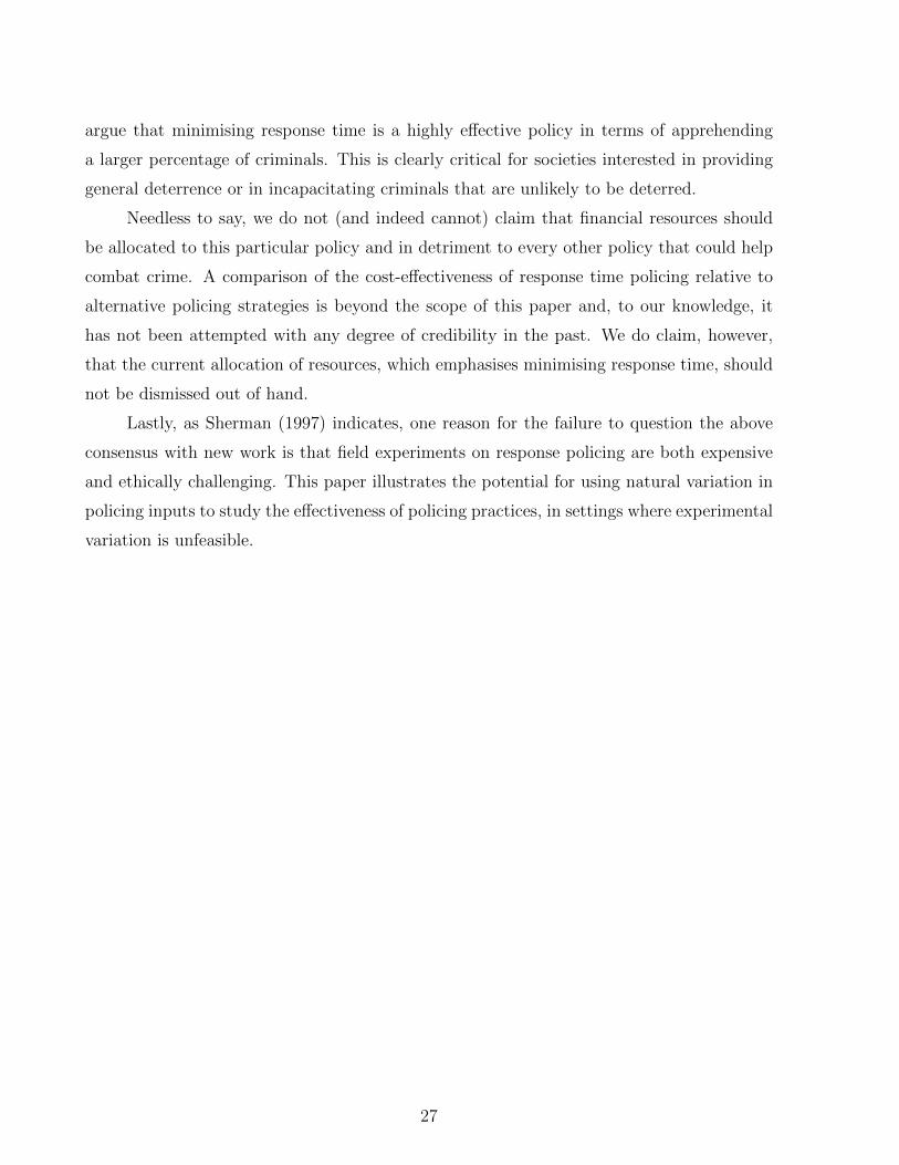
Around 38% of these crimes were detected, although, as we show in Figure 4, this percentage
varies considerably by Home Office classification code or by grade level. We can also see that
the response time distribution is highly skewed, with a mean of more than one hour and a
median of just 17 minutes. This skewness is confirmed in Figure 3, where we can see that
the density of the response time distribution peaks at around 5 minutes and falls concavely
after that.
Around 31% of calls are allocated a Grade 1 priority level. Theft offences represent
around half of all crimes (48%), followed by violent offences (23%) and criminal damage
(14%).
9The official definition of ’detection’ is as follows: ’A sanctioned detection occurs when (1) a notifiableoffence (crime) has been committed and recorded; (2) a suspect has been identified and is aware of thedetection; (3) the Crime Prosecution Service evidential test is satisfied; (4) the victim has been informed thatthe offence has been detected, and; (5) the suspect has been charged, reported for summons, or cautioned,been issued with a penalty notice for disorder or the offence has been taken into consideration when anoffender is sentenced.’ See http://data.london.gov.uk/dataset/percentage-detected-and-sanctioned-offences-borough.
11

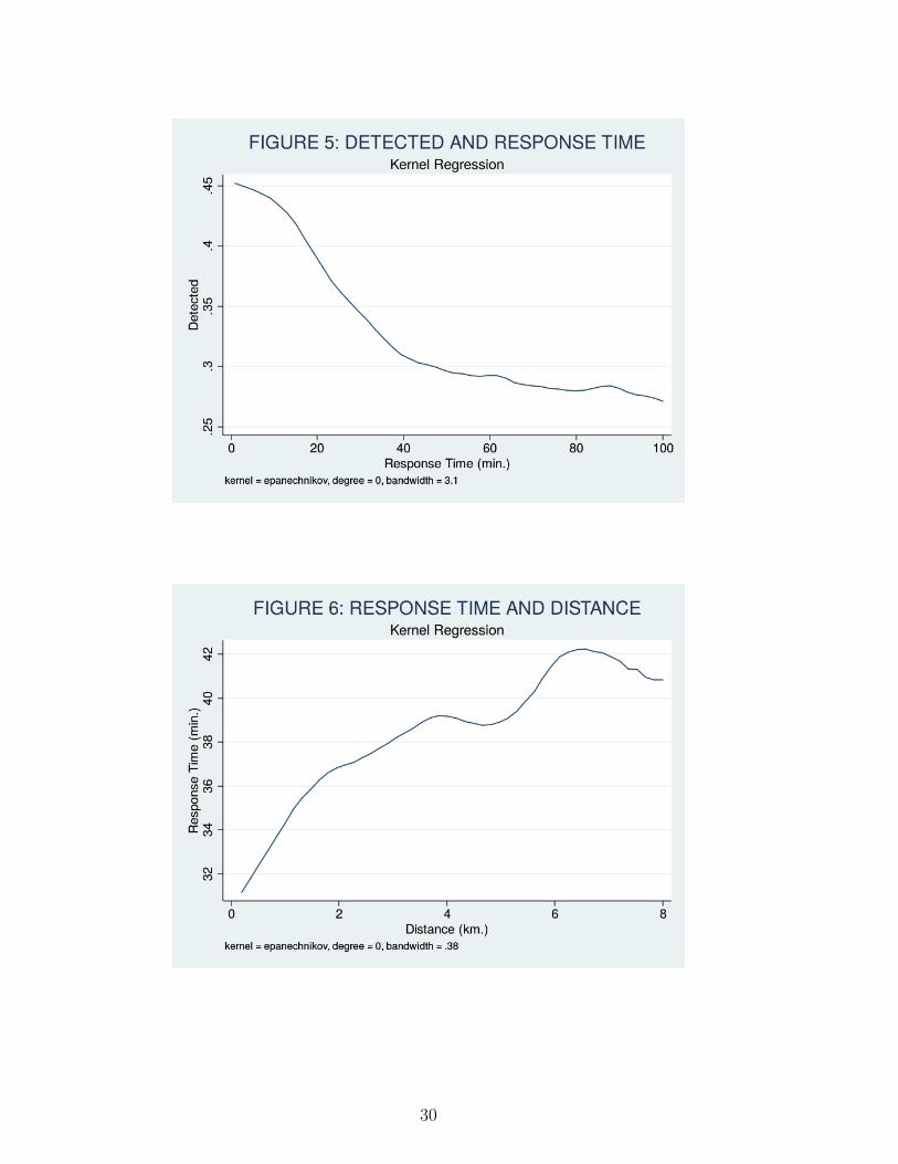
OLS Estimates Figure 5 displays a kernel regression of detection on response time10. In
addition to suggesting a negative relation, note that the shape of the relation appears strongly
concave. This seems unsurprising, as every extra minute should make a bigger difference
when response time is relatively fast. We will therefore use the log specification in our
main regressions below, although Table 6 shows that the baseline estimates are qualitatively
unchanged to measuring response time in levels.
Table 2 displays linear probability models of detection on (the log of) response time,
accounting for an increasingly richer set of controls. Our most exhaustive specification in
Column 5 controls for the hour of day in which the call was received, the division where the
crime occurred, the grade level assigned by the call handler, and the Home Office-classified
crime type. We find that faster response times are associated with a higher likelihood of
detection. The estimated effects suggest that a 10 percent decrease in response time is
associated with a .49 percentage points increase in the detection likelihood.
For several reasons we need to be cautious in giving the OLS estimates a causal in-
terpretation. Firstly, note that the information recorded by the handler during the call will
determine the priority it receives, and likely be correlated both with unobserved characteris-
tics of the crime and with the difficulty of detection. Secondly, response time may be directly
affected by the estimated likelihood of detection, in ways that are difficult to pin down. For
instance, response time may be particularly slow when a burglar is reported to have left the
scene long ago (low likelihood of detection), but also when a shoplifter has been detained by
a security guard (high likelihood), since in both cases the marginal effect of faster response
may be evaluated to be low. Lastly, response time may be correlated with other policing
inputs, such as the ability and attention of the responding officer. On the one hand, officers
who are less competent in other dimensions of the investigation may take longer to arrive at
the scene. Alternatively, it may be officers those who are aware of their low ability in other
dimensions that put more effort into responding quickly. It is difficult to draw conclusions
regarding the causal relation between response time and detection without a credible source
of exogenous variation in the former.
10The detection variable is time-censored, since the likelihood of solving a crime increases with time.However, the overwhelming majority of crimes are detected quite quickly, which makes this issue likelynegligible in our setting. To illustrate this, 58% of detections occur within the first week, 78% within thefirst month, and 96% within the first six months. We have therefore decided to ignore this potential problemin our regressions. We obtain very similar findings if we drop the last six months of 2014 from our dataset.
12

4 Empirical Strategy
In this section we explain in some detail the construction of our instrument for response
time. We first describe our measure of distance, discuss its potential as an instrument and
explore its empirical variation. We then explain why, after controlling for a large number of
small geographical cells, distance to the division response station could be regarded as a valid
instrument for response time. We also discuss potential threats to the exclusion restriction.
In the latter part of this section, we perform tests of exogeneity of our instrument and
interpret the corresponding results.
Distance and its Variation As we mentioned in Section 2, a call for service from a
Greater Manchester location needs to be responded by the division response team, i.e. the
team in the GMP division to which that location belongs. Our measure of distance is the
geodesic, or ’as the crow flies’, distance between the latitude and longitude of the crime scene
and the latitude and longitude of the closest division response station. Table 1 shows that
this measure is skewed to the right, with a mean of 3.2km. and a much lower median of
2.3km. We find in Figure 6 that the relation between response time and distance is strongly
positive and approximately linear. This finding provides a validation of our claim in Section
2 that response officers often depart from the division response station when called to attend
an incident.
Distance has been used as a source of exogenous variation by Reinikka and Svensson
(2005), Dittmar (2011), Dube et al. (2013) and Campante et al. (2014), among others. Its
validity as an instrument will obviously depend on the specific setting that is being studied.
In our setting caution is warranted, since crimes in different areas may differ in terms of their
detection difficulty. This could be by chance. For instance, it may be that response stations
tend to be located in city centres, and that crimes in these areas are easier or more difficult
to detect than crimes in suburban areas. The correlation between distance to the response
station and detection difficulty could also be by design. In particular, it may be that police
agencies choose to locate their response stations in high-crime, and perhaps high-difficulty-
crime, areas, so that they can minimise response time for crimes in these areas.
Intuition of the Instrument Locations that neighbour each other but are on different
sides of division boundaries are the responsibility of different response teams departing from
13

stations that will typically be located at different respective distances11. Our instrument is
based on the notion that, if we control with sufficient precision for the ’local area’ where
a crime occurs, the remaining variation in distance is mostly due to crime locations falling
on different sides of division boundaries and can therefore provide a source of exogenous
variation in response time.
In Figure 7, we clarify this intuition by displaying two geographical cells crossing
the boundary of two divisions. As we can see, the two marked locations in Cell 1 differ
significantly in the distance to their respective stations. And yet, these locations are next to
each other, and crimes occurring in them should have the same average detection difficulty.
The grid that we select for our baseline specifications covers the entire Greater Manch-
ester Area and it contains 5,152 unique cells of .005 by .005 decimal degrees (approximately
.185 squared kilometres or 556 metres by 332 metres)12. On average, around 504 people reside
in each cell13. Figure 7 superimposes two realistically-sized cells on the map of Manchester
and illustrates that only a handful of streets fit into a cell.
Accounting for Division Effects One reason that the two locations in Figure 7 differ
is, of course, that they belong to different divisions. This fact may be of concern, for two
reasons. Firstly, it may be that response teams in some divisions are simply better than
others at detecting crime, and that this is correlated with the average distance to the station
across divisions. For example, the response team of the (small) North Division may be
differently effective at detecting crime than its counterpart in the (large) Wigan Division
(see Figure 1). Secondly, division boundaries often coincide with political boundaries and
11To investigate compliance with this rule, we merged the location of all the crimes in our dataset withGMP-supplied shape files detailing the division boundaries. We then compared the division of the team thatresponded to a call with the division that, according to our shape files, should have officially responded.We found that they coincide in 99.31% of the crimes in our dataset, indicating that the official assignmentrule is followed in the vast majority of cases. The remaining .69% of cases could have been associated withdeviations from the official rule or, alternatively, may have been affected by measurement error in either thelocation variables or the division variable.
12At the latitude of Greater Manchester, a movement of .005 decimal degrees towards the equator repre-sents a higher number of metres than an equivalent movement in the direction of the Greenwich meridian,hence the rectangular shape of our cells. We chose the number of cells with the following procedure. Wefirst constructed a grid consisting of cells of .0005 squared degrees. We then tested whether, controlling forthese cell indicators, distance was still a strong predictor of response time. If the answer was yes, we dividedthe cells into 22 sub-cells, and estimated our first stage regression with the new set of cell indicators. Wecontinued until reaching the highest possible number of cells, consistently with a strong first stage that couldbe used to vary response time significantly. Our findings are robust to using a smaller or larger number ofcells, although the strength of the instrument obviously decreases if we increase the number of cells beyond5,152.
13For comparison, US census block groups have an average of 1,400 inhabitants.
14

this could have an independent effect on the difficulty of detection if the populations in
different local authorities are affected by different types of crimes. For these two reasons,
we need to ensure that any estimated effect of response time does not include the ’division
effects’ resulting from divisions (of potentially different size) having different types of crime
or levels of policing efficiency.
Figure 7 illustrates that these division effects can be separately identified from the
response time effect. For instance, because the two marked locations in Division F vary
in the distance to their response station, the addition of geographical cell indicators and
division indicators does not exhaust all the sample variation in distance. Our empirical
specifications will therefore always introduce a full set of division indicators.
Estimating Equations We use a 2SLS approach to estimate the effect of response time
on detection. The first stage equation between (the log of) response time and (the log of)
distance for crime i occurring in year t(i) in a location belonging to cell j(i) and division
d(i) is:
Responsei = α0 + α1Distancei + Cellj(i) × Y eart(i) +Divisiond(i) + Xi + εi (1)
where Xi is a vector of controls such as hour of day, grade level and Home Office classification
code indicators.
Note that the cell indicators are interacted with a set of year indicators. The reason
for this is as follows. Remember from Section 2 that the location of the response stations
changed across our sample period for some GMP divisions. These changes create time
variation in distance to the division station for a fixed location, even after controlling for
the cell indicators. For the reasons discussed in Section 2 this time variation is potentially
correlated with changes in crime patterns. We can, however, separate this time variation
from our preferred cross-sectional variation based on division boundaries by interacting the
cell indicators with a set of year indicators. After doing that, any variation in distance is
mostly due to crimes in the same cell/year falling on different sides of division boundaries
and therefore at different distances of their (fixed within a cell/year) response stations.
The second stage equation is:
Detectedi = β0 + β1 ˆResponsei + Cellj(i) × Y eart(i) +Divisiond(i) + Xi + υi (2)
where Detectedi is a dummy variable that takes value one if the crime was detected and
ˆResponsei captures the fitted values from (1).
15

In Appendix B we compare our empirical strategy with the strategies in other papers
such as Black (1999) and Doyle et al. (2015) that use boundary discontinuities for identifica-
tion. In particular, we comment on the differences in approach and explain why our current
strategy is well suited to the question and institutional setting of this paper.
Threats to Identification This empirical approach is subject to six main concerns. The
first is the possibility that the geographical cells may not be small enough, in which case the
assumption of homogeneity of locations within a cell will not be satisfied.
The second potential concern is the possibility of household sorting. For example,
households concerned about crime may decide to locate themselves on the side of the di-
vision boundary with the lowest police response times, in the same way that educationally
committed families have been shown to congregate in the catchment areas of good schools
(Black 1999, Bayer et al. 2007).
The third concern is due to potential sorting by criminals. If sophisticated criminals
target locations on the higher-distance side of a border, these locations will be associated with
more crimes, and with crimes that are more difficult to solve, posing a threat to identification.
The fourth concern is more subtle, and it has to do with the mechanical effect that
response time and the associated likelihood of arrest and imprisonment have on the com-
position of the criminal population. Namely, it may be that lower-distance locations are
depleted of some of their local criminals over time, and that the remaining criminals commit
crimes of higher or lower detection difficulty14.
The fifth concern is that a lower response time may affect not only the likelihood of
detection but also the nature of the crime itself. For instance, an immediate response may
prevent an attempted murder from becoming a murder or an assault from turning into an
aggravated assault. If different crime classifications require different standards for detection,
a faster response time may be affecting detection indirectly (through its effect on the type
of crime itself) as well as directly.
The last concern relates to the exclusion restriction integral to any 2SLS framework.
14This is probably not a big concern, for two reasons. Firstly, it relies on criminals being extremelyconsistent in their location decisions, for instance by always committing their crimes at home. If insteadthey cross division boundaries with a positive likelihood, the differential effect on the composition of thelocal criminal populations on opposite sides of the boundaries will be milder. Secondly, the United Kingdomhas relatively low incarceration rates, at least by U.S. standards. Differential incapacitation of criminals(and their associated effects on the composition of the local criminal populations) are therefore likely to besmall.
16

To adequately identify the effect of response time on detection, distance to the response
station must affect the likelihood of detection exclusively through the response time channel.
The concern arises because police stations that accommodate response teams typically also
contain the teams in charge of neighbourhood patrolling, and it is conceivable that crimes
in areas closer to a neighbourhood station may be more likely to be detected. For instance,
these areas may on average be patrolled more intensely. Alternatively, it may be that,
following spikes in crime, patrolling increases more in areas that are closer to a patrolling
station, perhaps because it is easier for the leadership of the neighbourhood teams to notice
increases in crime when these occur close to their base15. Lastly and most importantly, police
patrols may be more likely to stop at a crime scene to hear additional witnesses and gather
additional evidence if that scene is closer to the station from which they operate. This is
particularly important because neighbourhood officers are in charge of following up on the
investigation of the majority of crimes committed in Manchester.
In the remainder of this section, we undertake three separate balancing tests to evaluate
the empirical relevance of the first five concerns outlined above. In Section 5, we exploit the
fact that many patrolling stations are not response stations to examine the validity of the
exclusion restriction. To do this, we examine whether distance to patrolling stations (that
are neighbourhood non-response stations) is associated with a higher likelihood of detection.
Balancing Test 1: Household Demographics Our first test examines the first two
concerns outlined above. In particular, we want to examine empirically whether, controlling
for the cell and division indicators that are at the core of our empirical strategy, there is
any evidence that households located at different distances of their respective stations differ
in their demographic characteristics. To do this, we create a dataset of the 8,683 Greater
Manchester output areas, the smallest geographical areas in the 2011 UK census. Using the
latitude and longitude of every output area geographical centre, we assign it to a division,
and compute the distance to the 2014 closest response station. We also assign each output
area to a geographical cell. We then regress distance on a set of demographic characteristics,
controlling for the cell and division indicators. The estimated coefficients and confidence
intervals can be found in Figure 8.
To illustrate the value of our empirical strategy, we also display the equivalent esti-
15There is evidence that criminals who are not immediately arrested tend to reoffend within a few days inthe same area (Mastrobuoni, 2015). Heavier patrolling following a local spike in crime might then be morelikely to apprehend these repeat offenders.
17

mates and confidence intervals in a regression omitting the baseline set of cell and division
indicators. We find in Figure 8 that several demographic variables appear to be statistically
significant predictors of distance to the respective station at the output area level, when
cell and division controls are not included in the regression. For example, households living
further away from response stations are older, more likely to have children, and less likely to
have no qualifications. Controlling for cell and division indicators has two effects. Firstly, it
dramatically reduces the residual variance in the dependent variable (the adjusted R-squared
jumps from .06 to .98), leading to much lower standard errors. Secondly, we observe that the
estimated coefficients are now indistinguishable from zero (the F-statistic of joint significance
of the demographic variables decreases from 20.4 to 1.3).
We interpret the evidence in Figure 8 as indicating that output areas within the same
geographical cell contain households of similar demographic characteristics. This implies
that the geographical cells that we use are sufficiently small to ensure that locations within
each cell are identical in their observables, and therefore most likely in their unobservables.
It also indicates that the possibility of household sorting across division borders is unlikely.
Balancing Test 2: Total Number of Crimes Our second test evaluates jointly the
empirical relevance of the first five threats to identification. Every one of these hypotheses
predicts that the level of crime will be correlated with distance to the response station, even
after controlling for the cell and division indicators. To illustrate, consider the possibility
of sorting by criminals. If some criminals are sophisticated and target locations with slow
response time (including the high-distance side of division boundaries), then we should ob-
serve that locations further away from the station have more crime, both across and within
geographical cells.
To study whether this is an empirically relevant issue, we create a panel dataset of
census output areas and years, and compute the total number of crimes in each output
area and year combination. Again, we assign each output area/year to a division and to a
geographical cell. We then calculate the distance between the centre of each area and the
closest response station in that year. In Table 3, we regress one on the other, with and
without controlling for the cell/year and division indicators.
Column 1 shows that areas further away from the response station are associated
with less crime (the elasticity is -7.7% and strongly significant). Note by the way that this
finding is inconsistent with the notion that criminals target areas with slower response time.
18

The idea that criminals are sophisticated in their location decisions seems therefore to be
contradicted by the evidence. On the other hand, a negative elasticity is consistent with the
notion that the GMP choose to locate their response stations in high-crime areas16.
Importantly for the purposes of evaluating the validity of our empirical strategy, note
that the estimated elasticity decreases dramatically and becomes statistically insignificant
after we control for the cell/year and division indicators. We therefore interpret the evidence
in Table 3 as indicating that the first five threats to identification discussed above do not
seem empirically relevant.
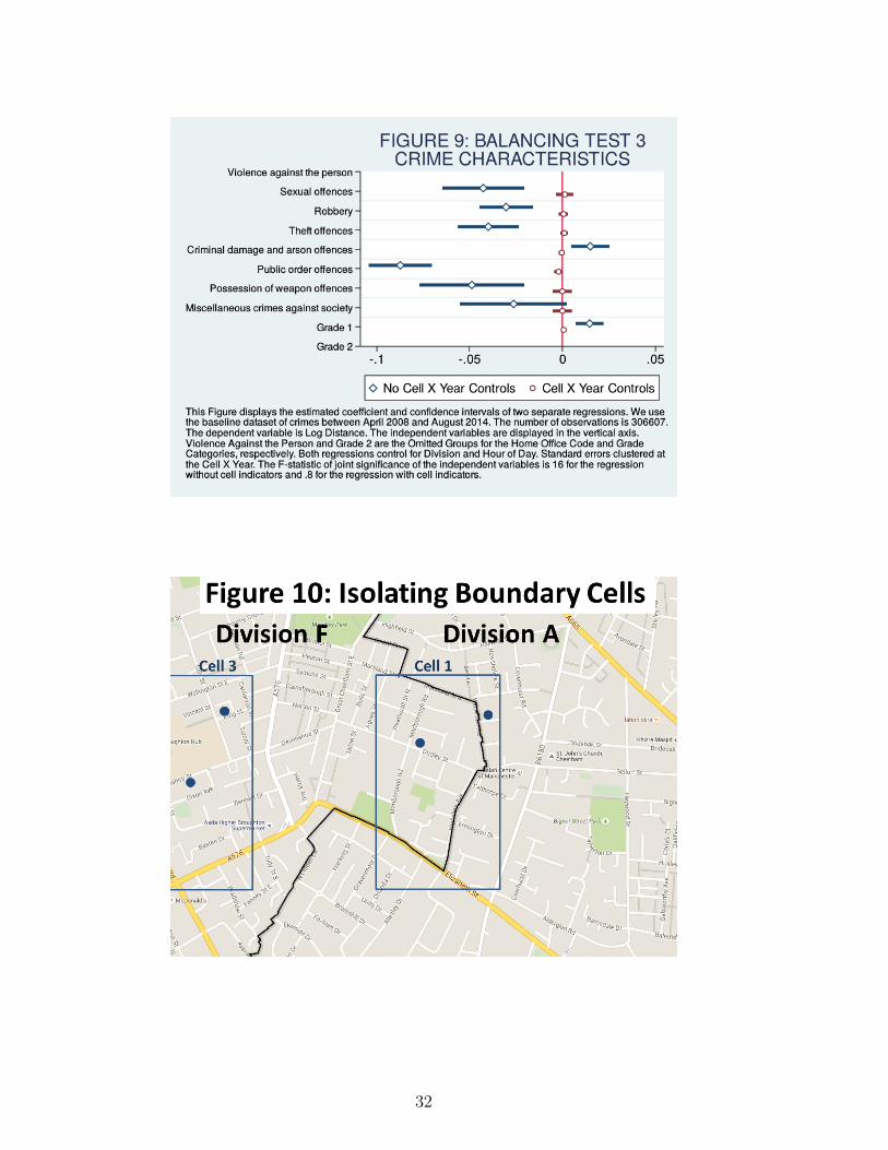
Balancing Test 3: Crime Characteristics All the first five threats to identification
predict that, conditional on a crime occurring, the type of crime should be correlated with
distance to the response station, even after controlling for the cell indicators. For instance, if
sorting by criminals is an empirically relevant issue, we would expect it to be more prevalent
among property crimes such as thefts than among violent crimes. This is because thieves
are widely regarded to be more sophisticated than violent criminals. Therefore, sorting
by criminals predicts that crimes occurring further away from the response station should
include a higher proportion of thefts, relative to violent offences.
To examine whether this is the case, we estimate the following empirical model on our
baseline dataset:
Distancei = π0 + Cellj(i) × Y eart(i) +Divisiond(i) + Xi + εi (3)
where Xi is our vector of interest, as it includes crime characteristics such as the UK Home
Office crime classification code and the grade level which are strongly correlated with the
likelihood of detection.
Figure 9 displays the coefficients and confidence intervals resulting from the estimation
of (3), again with and without cell/year and division controls. As we can see, the classification
code and grade level dummies are correlated with distance in the unconditional regression.
It is interesting to note, however, that the correlations seem inconsistent with the notion
that sophisticated criminals sort themselves away from the response station. In particular,
16An important difference between criminals and police agencies is that the latter have much betterinformation on which to base their decisions. For instance, they observe the locations of the responsestations and can experiment with them. They also have access to a large set of experience and hard dataregarding the relation between response time, distance and detection. Not even the most diligent criminalscan match that level of knowledge. We would therefore expect police agencies to be more sophisticated thancriminals in their location decisions.
19

theft offences are less numerous in locations further away from the response station, relative
to violent offences.
Controlling for the cell/year indicators has the same two effects as in Figure 8. Firstly,
the confidence intervals narrow significantly as a result of the decrease in the residual vari-
ance of the dependent variable (the adjusted R-squared of the regression jumps from .35 to
.98). Secondly, the estimated coefficients become essentially zero, despite the much narrower
confidence intervals. The F-statistic of a test of joint significance of the classification code
and grade level dummies also decreases dramatically from 16 to .8. We interpret the evidence
in Figure 9 as supporting the identification strategy in this paper.
5 Results
In this section we present and discuss the main results of the paper.
Naive IV Estimates Before displaying our baseline estimates, we show in Table 4 ’naive
IV’ coefficients, based on regressions that use distance to the response station as an instru-
ment but do not control for the cell/year indicators. We label these estimates naive based
on our findings from Figures 8 and 9 and Table 3 that distance is unlikely to be (uncon-
ditionally) orthogonal to the difficulty of detecting a crime. The reduced form estimate in
Column 1 suggests that crimes occurring 10% further away from the response station are
.48 percentage points less likely to be solved. In the second column we find the first stage
estimate. Reassuringly, the correlation between distance and response time that we first
identified in Figure 6 is robust to the inclusion of time, division and crime characteristics
indicators. The second stage coefficient is -.275, much larger than the OLS estimates.
Baseline Estimates We display the main results of the paper in Table 5. A compar-
ison with Table 4 shows that the reduced form estimate increases slightly, from -.048 to
-.065, when we introduce the cell/year controls. The first stage estimate is very strong (the
Kleibergen-Papp F statistic for weak identification is 53.11), and it suggests that a 10%
increase in distance to the response station is on average associated with a 1.40% increase in
response time. The second stage coefficient is -.464, approximately ten times larger than the
OLS estimate. The interpretation of the estimate is that a 10% increase in response time
leads to a 4.6 percentage points decrease in the likelihood of detection.
20

The most natural interpretation for the large gap between the OLS and the IV estimates
is that the bias associated with the OLS estimates is positive. In our setting, this implies
that crimes that are inherently more difficult to detect are given higher priority by the GMP,
and therefore benefit from faster response times17. This priority could also take the form of
response stations being endogenously located in high-difficulty crime areas. This would be
consistent with the evidence from Column 1 in Table 3 that the crime levels are higher in
areas close to the response station.
An alternative explanation for the difference in the OLS and IV estimates is that
the IV estimates are LATE, and capture the effect of response time on detection for the
compliant sub-population. In our setting the compliant crimes are those that would have
received a very fast response, had it not been for the fact that they are located far away
from the station. If response times are allocated optimally, these ’constrained’ crimes should
be precisely the ones for which the marginal return to a fast response is higher. Hence, the
large IV estimate may be the result of the fact that the LATE compliant crimes are those
with the largest marginal return to a fast response.
Robustness to Introducing Response Time and Distance in Levels Throughout
this paper we have introduced response time and distance in logarithmic form. This is firstly
for theoretical reasons, since we would expect an extra minute in response time to have a
bigger effect when response time is relatively fast. Our choice of functional form is also
motivated by our evidence in Figure 5 that the relation between response time and detection
appears strongly concave.
Nevertheless, we find in Table 6 qualitatively similar results when we introduce both
response time and distance in levels18. The reduced form estimate in Column 1 indicates that
every extra kilometre in distance between a crime scene and the division response station
leads to a 1.8 percentage points decrease in the detection likelihood. The first stage esti-
mate is again positive and statistically significant, although it leads to a weaker instrument
(Kleibergen-Papp F statistic of 10.74). An extra kilometre in distance is associated with an
17Our discussions with police officers in the GMP revealed that there is no career penalty for beingassociated with unsolved crimes, at least at the officer level. This would be consistent with officers notshying away from responding to seemingly difficult-to-solve crimes.
18The distribution of response time has a relatively large number of outlying observations, which havea disproportionate effect on any regression in levels. Therefore, we decided to drop observations with aresponse time of more than 500 minutes (this is more than 8 times the target response time for Grade 2calls). We find very similar results when using other common strategies to deal with outlying observations.
21

average of 1.75 extra minutes in response time. The second stage estimate is statistically
significant at the 5% level and indicates that an extra minute in response time leads on
average to a 1 percentage point decrease in detection likelihood.
Robustness to the Sequential Introduction of Controls Given that our instrument
is supposed to induce exogenous variation in response time, the estimated coefficients should
not be sensitive to the inclusion or exclusion of other control variables. In Tables 7 and
8 we examine whether this is the case, respectively for the reduced form and second stage
estimates. We introduce sequentially the hour of the day in which the police was alerted
to the crime, the call handler’s grade level and the Home Office classification code. The
estimates appear remarkably robust to the set of controls in the regression. This is consistent
with our finding in Figure 8 that distance is (conditionally) uncorrelated with these controls.
We interpret Tables 7 and 8 as providing reassurance with regards to our baseline estimates
in Table 5.
Robustness to Using Only Variation from Boundary Cells Our second specification
check is more subtle. The need for it is perhaps best understood by looking at Figure 10. Our
identification strategy exploits variation in distance controlling for a large set of very small
geographical cells. A large part of this variation is coming, as we have argued throughout
this paper, from cells that cross division boundaries, such as Cell 1 in Figure 10. However,
some variation in distance is also due to locations that are slightly apart from each other and
in the same cell and division (i.e. the two locations pictured in Cell 3). Arguably, this last
type of variation is very small in magnitude, given that the cells are very small. Nevertheless,
we want to test the robustness of our baseline estimates to a specification that strictly uses
only variation in distance across locations in ’boundary cells’.
This can be done in a 2SLS framework simply by interacting distance and response
time with a ’boundary cell’ dummy. In Table 9 we do this and find that the coefficients are
similar to our baseline estimates. The reduced form estimate is slightly larger at -.07 and
the first stage coefficient is also larger at .178. The second stage estimate is very similar at
.395. We interpret this evidence as reinforcing the main conclusion of the paper.
Evidence on Non-Response Patrolling Stations As we mentioned in Section 4, re-
sponse stations are also the base stations from which some neighbourhood teams operate.
22

This is a concern because it may be that it is the distance to the base station of a neighbour-
hood team (rather than the distance to the base station of a response team) that causes the
differential likelihood of detection that we have identified above. The main reason why this
may happen is that, for the vast majority of crimes, neighbourhood officers are in charge
of following up on the preliminary investigations conducted by the response officers attend-
ing a crime scene. Perhaps these subsequent investigations are somehow conducted more
thoroughly when the crime scenes are closer to the neighbourhood team stations19.
To examine the plausibility of this alternative channel, we take advantage of the fact
that the divisions in the GMP contain a large number of police stations with a neighbourhood
team but without a response team. We can test the validity of the exclusion restriction
by examining whether distance to a neighbourhood (but non-response) station is similarly
predictive of the likelihood of detection. We create this new measure in exactly the same
way as the distance to a response station described in Section 4, and display the results in
Table 10.
We first find that the reduced form effect of distance to a non-response patrolling station
is essentially zero. Note also that the standard errors are small, so the effect is precisely
estimated. In the second column, we find that response time is uncorrelated with distance to
a non-response station as we would expect. The effect of distance to a non-response station
is also essentially zero when we instrument response time with the distance to a response
station. These findings suggest that proximity to a response station increases the likelihood
of detection by decreasing response time, rather than by affecting the behaviour of the local
neighbourhood team.
Heterogeneity We now examine whether the effects of response time on detection differ
across types of crime. To do this, we create sets of dummies that split the population of
crimes along several dimensions and interact these dummies with response time in (2) and
with distance in (1)20.
19However, note that when we suggested this possibility to several neighbourhood officers in the GMP,the overwhelming response was that this was highly implausible.
20Alternatively, we could run (1) and (2) separately for every type of crime. Due to the large number ofcontrol indicators and to the fact that variation in distance to the response station is based on a relativelysmall number of observations, this strategy leads to very weak instruments. We have therefore decided toimpose the assumption that the control variables do not have a differential effect by type of crime. Everyresult in this section must be interpreted with this caveat in mind. Note also that, to preserve the strengthof the instruments, we have divided the population of crimes into only two or three groups at a time. Thethree panels in Table 11 should therefore not be interpreted as the outcomes of independent tests.
23

We start by examining how the estimated coefficients vary across grade level. Remem-
ber from Section 2 that Grade 1 calls are typically those where there is an imminent threat
to someone’s safety or where a crime is taking place. Grade 2 calls are those where there
is no imminent threat but key evidence or witnesses are likely to be lost if attendance is de-
layed (Police and Crime Commissioner, 2013). Because Grade 2 calls are explicitly defined
as those for which a fast response is likely to matter most (in terms of crime detection), we
would expect Grade 2 calls to be associated with a higher coefficient than Grade 1 calls.
This is indeed what we find in Panel A of Table 10. As we can see, Grade 2 calls have an
estimated coefficient of -.484, which is slightly larger than the -.397 estimate for Grade 1
calls (and statistically different at the 10% level).
In Panel B we explore the heterogeneity of the coefficients in terms of the time delay
between the crime occurring and the police being alerted. This exercise is motivated by
Pate et al. (1976) and Spellman and Brown (1981), who argue that, because it takes a long
time for the victims to call the police, any improvement in police response time is unlikely
to make a difference. We define the call delay as the number of minutes between the end
point of the crime and the police receiving the phone call. Unfortunately, GMP records
regarding the end time of crimes are likely subject to a lot of measurement error, since they
are typically based on the estimates and recollections of victims and witnesses. Furthermore,
this information is missing for approximately a quarter of crimes. Nevertheless, we display
the density of the call delay variable in Figure 11. We find that, contrary to the early 70s
findings of Pate et al. (1976) and Spellman and Brown (1981), the typical call delay is very
short, at least in our dataset. In Figure 11, we can see that the density of the call delay
variable peaks at around 1 minute and becomes very low after 20 minutes. The median of
the call delay distribution is slightly over 4 minutes (Table 1) and the 33rd and 66th centiles
are 1 and 13 minutes respectively. Furthermore, it takes negative values for approximately
18% of observations, indicating that the police was alerted even before the crime stopped
taking place.
In Panel B of Table 11 we split the sample into thirds and find that police response
time has a statistically identical effect regardless of the call delay. This is an issue that
merits future investigation, hopefully with more precise data. At this point we can offer
two interpretations of this finding. Firstly, the lack of differences in the estimated effects
may simply be due to the likely measurement error in the call delay variable. The second
explanation is based on the fact that, in order to be assigned a Grade 1 or Grade 2 priority
24

level, a call needs to be regarded as sufficiently urgent by the call handler. In other words,
even calls in our sample with a relatively high call delay have passed the hurdle of meriting
the prompt attendance of a response officer, perhaps because the effect of response time on
detection was evaluated to be large. Given this fact, it may not be so surprising to find that
even crimes with a high call delay benefit similarly from a fast response.
Effect on the Intensive Margin: Time to Detection One way to interpret the ev-
idence above is that response times have an effect on the extensive margin of the police
production function, since faster response times can turn potentially undetected crimes into
detected crimes. We now proceed to examine whether response times also have an effect on
the detection intensive margin, in terms of reducing the time that it takes to detect crimes.
To do this, we restrict the sample to crimes that were detected by August 2014, and use our
baseline empirical specification to study whether faster response times are associated with
faster detection times.
The second column of Table 12 shows that the estimated relation between response
time and distance is very similar in the subsample of detected crimes relative to that in the
overall sample (12.2% versus 14%). The smaller size of the sample leads, however, to a much
weaker instrument than in the baseline regressions of Table 5 (Kleibergen-Papp F-statistic
of 13.82).
The reduced form estimate in Column 1 and the second stage estimate in Column 3
both indicate that a crime will be solved more quickly (conditional on it being solved at
all) if the police reach the crime scene more promptly after being alerted. The estimated
elasticity in Column 3 is economically large: a 10% increase in response time will lead to a
9.07% increase in the time that it takes to detect a crime (in addition to the possibility that
it may never be detected at all). If ’justice delayed is justice denied’, we cannot think of the
extra time to detection as an additional detrimental effect of reaching a crime scene too late.
Mechanism In Section 2 we discussed potential mechanisms through which fast response
time could make a difference. To reiterate, we mentioned that the police could arrest the
offender either at the scene of the crime or in its vicinity; they could collect physical evidence
before it is contaminated or destroyed; they could interrogate witnesses before they have left
the scene and they could encourage victim or witness cooperation by signaling efficiency and
dedication. We now explore empirically the importance of the last two mechanisms: victim
25

or witness availability and cooperation in terms of naming a suspect.
In our dataset, we have information on whether a suspect was named to the police21.
It seems obvious that the chances of detecting a crime will improve strongly if the police
receive such information. Isaacs (1967), Chaiken et al. (1977) and Greenwood (1980), for
instance, find that a much larger percentage of cases are cleared if the police have a named
suspect. This is also the case in our dataset. Among the 24% of crimes where there is a
named suspect, 65% of crimes are detected, whereas in the remaining 76% the likelihood of
detection rate is only 29%.
Our hypothesis is that a suspect will be named relatively more often when the police
is faster in attending the scene. To examine this, we display in Table 13 a version of (2)
where the dependent variable is a dummy indicating whether a suspect was named to the
police (the first stage equation is unchanged). We indeed find that faster response times
lead to a higher likelihood of this type of cooperation by a victim or witness. The reduced
form estimate is also negative and statistically significant. We conclude that this is indeed
a mechanism through which faster response times have an effect on crime detection.
6 Discussion
In this paper we have provided robust evidence of a causal effect of police response time
on crime detection. The estimated effects are large and strongly significant. They hold on
the extensive margin (likelihood of detection) as well as on the intensive margin (time to
detection). We find stronger effects for thefts than for violent offenses, although the effects
are large for every type of crime. The effects are larger for incident calls that are given
higher priority by the GMP on the grounds that the likelihood of detection may decrease
if response time is slow (i.e. Grade 2 crimes). Lastly, we have provided some evidence on
one of the mechanisms through which police response time operates: the likelihood that a
victim or witness will name a suspect to the police.
Our findings contradict long-standing beliefs among criminologists regarding the ef-
fectiveness of rapid response policing. While the existing consensus is that rapid response
policing has either a zero or at best a very weak effect on the likelihood of detection, we
21Unfortunately, we do not observe who named such a suspect or whether the suspect was confirmedas the person responsible for the crime. We do not observe either the variables necessary to explore theother potential mechanisms, such as the quality of the physical evidence gathered or the accuracy of witnessrecollections.
26
argue that minimising response time is a highly effective policy in terms of apprehending
a larger percentage of criminals. This is clearly critical for societies interested in providing
general deterrence or in incapacitating criminals that are unlikely to be deterred.
Needless to say, we do not (and indeed cannot) claim that financial resources should
be allocated to this particular policy and in detriment to every other policy that could help
combat crime. A comparison of the cost-effectiveness of response time policing relative to
alternative policing strategies is beyond the scope of this paper and, to our knowledge, it
has not been attempted with any degree of credibility in the past. We do claim, however,
that the current allocation of resources, which emphasises minimising response time, should
not be dismissed out of hand.
Lastly, as Sherman (1997) indicates, one reason for the failure to question the above
consensus with new work is that field experiments on response policing are both expensive
and ethically challenging. This paper illustrates the potential for using natural variation in
policing inputs to study the effectiveness of policing practices, in settings where experimental
variation is unfeasible.
27

FIGURES
28
29
30

31
32

33

TABLES
Table 1: SUMMARY STATISTICSVariable Obs Mean Std. Dev. Min Max P50
Detected 306607 .376 .484 0 1 0Suspect Named 306607 .237 .426 0 1 0Time to Detection (days) 105419 34.474 113.436 0 2218 4Response Time (min.) 306607 73.298 315.015 .067 21613.58 16.817Distance to Station (km.) 306607 3.248 3.678 .004 18.999 2.256Call Delay (min.) 232558 3960.98 184155.9 -38109.58 2.42e+07 4.055Grade 1 306607 .308 .462 0 1 0Grade 2 306607 .692 .462 0 1 1Violent Offenses 306607 .229 .42 0 1 0Sexual Offenses 306607 .014 .118 0 1 0Robbery 306607 .052 .221 0 1 0Theft Offenses 306607 .478 .5 0 1 0Criminal Damage/Arson 306607 .143 .35 0 1 0Public Order Offenses 306607 .065 .247 0 1 0Possession of Weapon 306607 .009 .095 0 1 0Miscellaneous against Society 306607 .01 .098 0 1 0
TABLE 2: OLS ESTIMATESDetected and Response Time(1) (2) (3) (4) (5)
VARIABLES Detected Detected Detected Detected Detected
Log Response Time -0.053*** -0.059*** -0.049*** -0.048*** -0.049***(0.001) (0.001) (0.001) (0.001) (0.001)
HourOfDay No Yes Yes Yes YesGrade No No Yes Yes YesHomeOfficeCode No No No Yes YesDivision No No No No Yesr2 0.0235 0.0419 0.0436 0.0883 0.0932N 306607 306607 306607 306607 306607
Robust Standard Errors in Parentheses.
34

TABLE 3: BALANCING TEST 2 (TOTAL CRIMES)Log Number of Crimes on Log Distance
(1) (2)VARIABLES LogCrimes LogCrimes
(Log) Distance -0.077*** 0.002(0.006) (0.007)
CellXYear No YesDivision No Yesr2 0.00469 0.664N 58762 58762
An observation is a UK census output area and year combination.
Standard Errors in Parentheses Clustered by Cell X Year.
TABLE 4: NAIVE IV ESTIMATESInstrument = Distance (Without Cell X Year Indicators)
(1) (2) (3)ReducedForm FirstStage SecondStage
VARIABLES Detected Log Response Time Detected
Log Distance -0.048*** 0.174***(0.001) (0.003)
Log Response Time -0.275***(0.008)
N 306607 306607 306607widstat 3655
All Regressions Control for HourOfDay, Year, Division, Grade and Home Office Code.
Standard Errors clustered by Day X Hour.
widstat= Kleibergen-Papp F statistic for weak identification
35

TABLE 5: BASELINE IV ESTIMATESInstrument = Distance (With Cell X Year Indicators)
(1) (2) (3)ReducedForm FirstStage SecondStage
VARIABLES Detected Log Response Time Detected
Log Distance -0.065*** 0.140***(0.012) (0.019)
Log Response Time -0.464***(0.098)
N 306607 306607 306607widstat 53.11
All Regressions Control for Cells X Year, HourOfDay, Division, Grade and Home Office Code.
Standard Errors Clustered by Cell X Year.
widstat= Kleibergen-Papp F statistic for weak identification
TABLE 6: IV ESTIMATES IN LEVELSInstrument = Distance (With Cell X Year Indicators)
(1) (2) (3)ReducedForm FirstStage SecondStage
VARIABLES Detected Response Time (min.) Detected
Distance (km.) -0.018*** 1.753***(0.005) (0.535)
Response Time (min.) -0.010**(0.004)
N 298208 298208 298208widstat 10.74
All Regressions Control for Cells X Year, HourOfDay, Division, Grade
and Home Office Code. Standard Errors Clustered by Cell X Year.
widstat= Kleibergen-Papp F statistic for weak identification
36

TABLE 7: ROBUSTNESS OF REDUCED FORM REGRESSIONSDetected on Distance (With Cell X Year Indicators)
(1) (2) (3) (4)VARIABLES Detected Detected Detected Detected
Log Distance -0.070*** -0.068*** -0.069*** -0.065***(0.007) (0.007) (0.007) (0.007)
HourOfDay No Yes Yes YesGrade No No Yes YesHomeOfficeCode No No No Yesr2 0.208 0.211 0.226 0.266N 306607 306607 306607 306607
All regressions control for Division and Cells X Year.
Standard Errors in Parentheses Clustered by Cells X Year.
TABLE 8: ROBUSTNESS OF IV REGRESSIONSInstrument = Distance (With Cell X Year Indicators)
(1) (2) (3) (4)VARIABLES Detected Detected Detected Detected
Log Response Time -0.580*** -0.510*** -0.483*** -0.464***(0.161) (0.120) (0.094) (0.098)
HourOfDay No Yes Yes YesGrade No No Yes YesHomeOfficeCode No No No YesN 306607 306607 306607 306607widstat 23.13 32.70 53.80 53.11
All regressions control for Division and Cells X Year.
Standard Errors in Parentheses Clustered by Cells X Year.
widstat= Kleinbergen-Papp F statistic for weak identification
37

TABLE 9: IV ESTIMATES (ONLY BOUNDARY CELLS)Instrument = Distance X Boundary (With Cell X Year Indicators)
(1) (2) (3)ReducedForm FirstStage SecondStage
VARIABLES Detected Log Response Time Detected
Log Distance X Boundary -0.070*** 0.178***(0.021) (0.042)
Log Response Time -0.395***(0.132)
N 306607 306607 306607widstat 18.31
All Regressions Control for Log Distance X Single-Division Cell, Cell X Year, Hour of Day, Division, Grade
and Home Office Code. Standard Errors Clustered by Cell X Year.
widstat= Kleibergen-Papp F statistic for weak identification
TABLE 10: INCLUDING NON-RESPONSE POLICE STATIONSInstrument = Distance (With Cell X Year Indicators)
(1) (2) (3)ReducedForm FirstStage SecondStage
VARIABLES Detected Log Response Time Detected
Log Distance -0.064*** 0.143***(0.012) (0.019)
Log Distance Non-Response -0.002 0.026 0.009(0.006) (0.016) (0.009)
Log Response Time -0.446***(0.097)
N 306607 306607 306607widstat 53.74
All Regressions Control for Cells X Year, HourOfDay, Division, Grade and Home Office Code.
Standard Errors Clustered by Cell X Year.
widstat= Kleibergen-Papp F statistic for weak identification
38
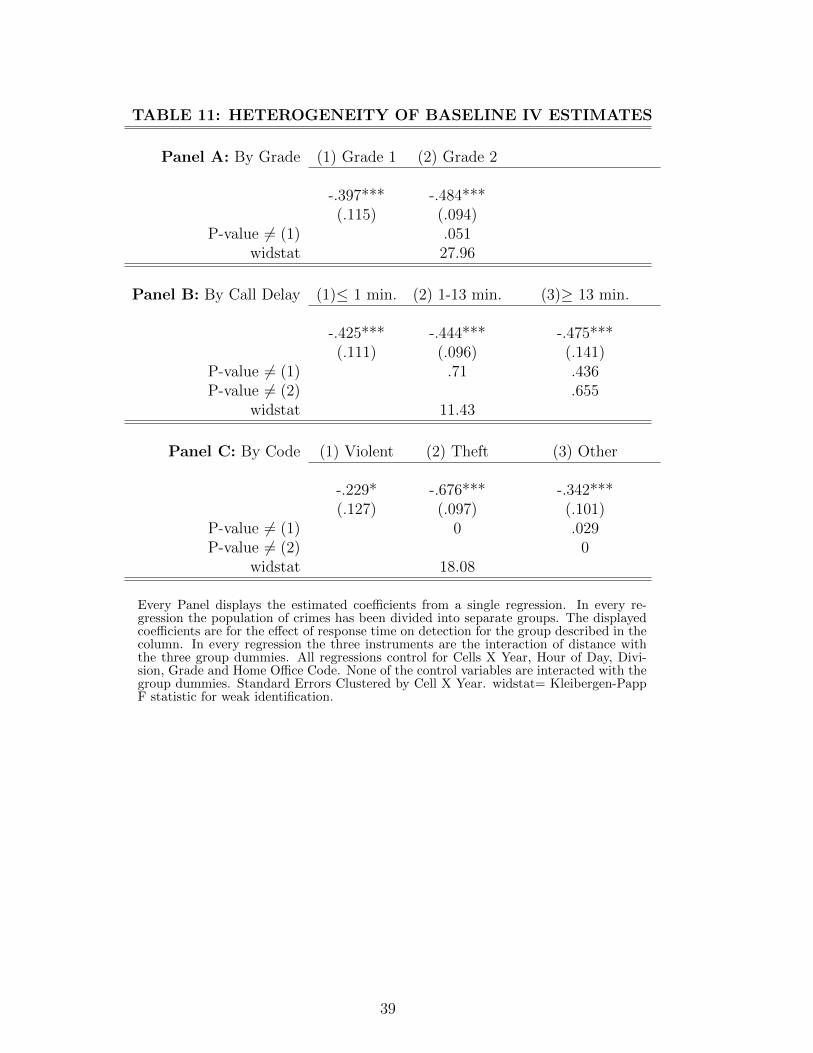
TABLE 11: HETEROGENEITY OF BASELINE IV ESTIMATES
Panel A: By Grade (1) Grade 1 (2) Grade 2
-.397*** -.484***(.115) (.094)
P-value 6= (1) .051widstat 27.96
Panel B: By Call Delay (1)≤ 1 min. (2) 1-13 min. (3)≥ 13 min.
-.425*** -.444*** -.475***(.111) (.096) (.141)
P-value 6= (1) .71 .436P-value 6= (2) .655
widstat 11.43
Panel C: By Code (1) Violent (2) Theft (3) Other
-.229* -.676*** -.342***(.127) (.097) (.101)
P-value 6= (1) 0 .029P-value 6= (2) 0
widstat 18.08
Every Panel displays the estimated coefficients from a single regression. In every re-gression the population of crimes has been divided into separate groups. The displayedcoefficients are for the effect of response time on detection for the group described in thecolumn. In every regression the three instruments are the interaction of distance withthe three group dummies. All regressions control for Cells X Year, Hour of Day, Divi-sion, Grade and Home Office Code. None of the control variables are interacted with thegroup dummies. Standard Errors Clustered by Cell X Year. widstat= Kleibergen-PappF statistic for weak identification.
39

TABLE 12: IV ESTIMATES (DEP. = TIME TO DETECTION)Instrument = Distance X Boundary (With Cell X Year Indicators)
(1) (2) (3)ReducedForm FirstStage SecondStage
VARIABLES LogTimeToDetection Log Response Time LogTimeToDetection
Log Distance 0.111** 0.122***(0.052) (0.033)
Log Response Time 0.907*(0.484)
N 105419 105419 105419widstat 13.82
All Regressions Control for Cells X Year, HourOfDay, Division, Grade and Home Office Code.
Sample Contains Only Detected Crimes. Standard Errors Clustered by Cell X Year.
widstat= Kleibergen-Papp F statistic for weak identification
TABLE 13: IV ESTIMATES (DEP. = SUSPECT NAMED)Instrument = Distance (With Cell X Year Indicators)
(1) (2) (3)ReducedForm FirstStage SecondStage
VARIABLES S.Named Log Response Time S.Named
Log Distance -0.020** 0.140***(0.009) (0.019)
Log Response Time -0.141**(0.069)
N 306607 306607 306607widstat 53.11
All Regressions Control for Cells X Year, HourOfDay, Division, Grade and Home Office Code.
Standard Errors Clustered by Cell X Year.
widstat= Kleibergen-Papp F statistic for weak identification
40

REFERENCES
Adda, J., McConnell, B., and Rasul, I. (2015), “Crime and the Depenalization ofCannabis Possession: Evidence from a Policing Experiment”, Journal of Political Economy,122(5), 1130-1202.
Bayer, P., Ferreira, F., and McMillan, R. (2007), “A unified framework formeasuring preferences for schools and neighborhoods (No. w13236)”, National Bureau ofEconomic Research.
Bayley, D. H. (1996), “Police for the Future”, New York: Oxford University Press.Becker, C. (1968), “Punishment: An Economic Approach”, 76 Journal of Political
Economy, 169(10.2307), 1830482169.Benson, B. L., and Rasmussen, D. W. (1991), “Relationship between illicit drug
enforcement policy and property crimes”, Contemporary Economic Policy, 9(4), 106-115.Black, S. E. (1999), “Do better schools matter? Parental valuation of elementary
education”, Quarterly Journal of Economics, 577-599.Blundell, J. (2007), “Policing a liberal society”, Economic Affairs, 27(4), 4-11.Braga, A. A. (2001), “The effects of hot spots policing on crime”, The ANNALS of
the American Academy of Political and Social Science, 578(1), 104-125.Bratton, W., and Knobler, P. (2009), “The turnaround: How America’s top cop
reversed the crime epidemic”, London: Random House.Campante, F. R. (2014), “Isolated Capital Cities, Accountability, and Corruption:
Evidence from US States”, The American Economic Review, 104(8), 2456-2481.Chaiken, J. M., Greenwood, P. W., and Petersilia, J. (1977), “The criminal
investigation process: A summary report”, Policy Analysis, 187-217.Clawson, C. and Chang, S. (1975), “Impact of response delay on arrest rates”,
Inspectional Services Division, Seattle Police DepartmentCollege of Policing (2013), “Investigation: Investigation Process ”, available at:
https://www.app.college.police.uk/app-content/investigations/investigation-process/Cordner, G. W., and Scarborough, K. E. (2010), “Police administration ”New
Providence: Routledge.Davis, R. C. (2012), “Selected international best practices in police performance
measurement ”, Rand Corporation.DeAngelo, G, and Owens E. G. (2014), “Learning the Ropes: Task Specific Expe-
rience and the Output of Idaho State Troopers”, Working Paper.Dempsey, J., and Forst, L. (2011), “An introduction to policing ”Boston: Cengage
Learning.Di Tella, R., and Schargrodsky, E. (2004), “Do police reduce crime? Estimates
using the allocation of police forces after a terrorist attack”, The American Economic Review,94(1): 115-133.
Dittmar, J. E. (2011), “Information technology and economic change: the impact ofthe printing press”, The Quarterly Journal of Economics, 126(3): 1133-1172.
Doyle, J., Graves, J., Gruber, J., and Kleiner, S. (2015), “Measuring returns tohospital care: Evidence from ambulance referral patterns”, The Journal of Political Econ-omy, 123(1), 170.
41

Draca, M., Machin, S., and Witt, R. (2011), “Panic on the streets of london:Police, crime, and the july 2005 terror attacks”, The American Economic Review, 2157-2181.
Dube, A., Dube, O., and Garca-Ponce, O. (2013), “Cross-border spillover: USgun laws and violence in MexicoContracts”, American Political Science Review, 107(03):397-417.
Ehrlich, I. (1973), “Participation in illegal activities: a theoretical and empiricalinvestigation”, Journal of Political Economy, 81(3): 521-65.
Evans, W. N., and Owens, E. G. (2007), “COPS and Crime”, Journal of PublicEconomics, 91(1): 181-201.
Frydl, K., and Skogan, W. (Eds.) (2004), “Fairness and Effectiveness in Policing::The Evidence ”Washington D.C.: National Academies Press.
Garicano, L., and Heaton, P. (2010), “Information technology, organization, andproductivity in the public sector: evidence from police departments”, Journal of LaborEconomics, 28(1): 167-201.
Greenwood, P. W. (1980), “The Rand study of criminal investigation: the findingsand its impact to date”, The effectiveness of policing, 35-43.
Goldstein, H. (1990), “Problem-oriented policing”, New York: McGraw-Hill.Hess, K. and Hess Orthmann, C. (2012), “Criminal investigation”, 10th edition,
Clifton Park: Cengage Learning.Hoxby, C. M. (2000), “Does competition among public schools benefit students and
taxpayers? ”, American Economic Review, 1209-1238.Isaacs, H. (1967), “A study of communications, crimes, and arrests in a metropolitan
police department”, Task Force report: science and technology, 88-106.Karn, J. (2013), “Policing and crime reduction: The evidence and its implications for
practice ”, Washington DC: Police Foundation.Katz, C. M. and Walker, S. (2012), “Police in America”, New York: McGraw-Hill.Kelling, G. L., Pate, T., Dieckman, D., and Brown, C. E. (1974), “The Kansas
City preventive patrol experiment: A summary report (Vol. 1015)”, Washington DC: PoliceFoundation.
Kennedy, D. M. (1993), “The strategic management of police resources”, US De-partment of Justice, Office of Justice Programs, National Institute of Justice.
Klick, J., and Tabarrok, A. (2005), “Using Terror Alert Levels to Estimate theEffect of Police on Crime”, Journal of Law and Economics, 48(1): 267-279.
Levitt, S. D. (1997), “Using electoral cycles in police hiring to estimate the effect ofpolice on crime”, The American Economic Review,270-290.
Mastrobuoni, G. (2014), “Crime is Terribly Revealing: Information Technology andPolice Productivity”, forthcoming.
Mastrobuoni, G. (2015), “Police and clearance rates: Evidence from recurrent rede-ployments within a city”, working paper.
McCrary, J. (2002), “Using Electoral Cycles in Police Hiring to Estimate the Effectof Police on Crime: Comment”, The American Economic Review,92(4): 1236-1243.
McCrary, J. (2007), “The effect of court-ordered hiring quotas on the compositionand quality of police”, The American Economic Review, 318-353.
42

Miller, A. R., and Segal, C. (2014), “Do female officers improve law enforcementquality? Effects on crime reporting and domestic violence escalation. Effects on CrimeReporting and Domestic Violence Escalation”, working paper, (September 16, 2014).
Pate, T., Ferrara, A., Bowers, R. A., and Lorence, T. (1976), “Police responsetime: its determinants and effects Police Foundation”, Washington DC: Police Foundation.
Police and Crime Commissioner for Greater Manchester (2013), “GM Office ofthe Police and Crime Commissioner Briefing Paper: Operational Communications Briefing”,available athttps://meetings.gmpcc.org.uk/documents/s6161/PCC%20OCB%20Briefing%20December%202013%20v0.6.pdf
Reinikka, R., and Svensson, J. (2005), “Fighting corruption to improve school-ing: Evidence from a newspaper campaign in Uganda”, Journal of the European EconomicAssociation, 3(23): 259-267.
Shavell, S. (1987), “A model of optimal incapacitation”, The American EconomicReview, 107-110.
Sherman, L. W. (2013), “The rise of evidence-based policing: Targeting, testing, andtracking”, Crime and Justice,42(1): 377-451.
Sherman, L. W., and Eck, J. E. (2002), “Policing for crime prevention”, inEvidence-based crime prevention London: Routeledge.
Sherman, L. W., Gottfredson, D., MacKenzie, D., Eck, J., Reuter, P., andBushway, S. (1997), “Preventing crime: What works, what doesnt, whats promising: Areport to the United States Congress prepared for the National Institute of Justice ”, Wash-ington, DC.
Siegel, L., and Worrall, J. (2014), “Essentials of criminal justice”, Clifton Park:Cengage Learning.
Soares, R. R., and Viveiros I. (2010), “Organization and information in the fightagainst crime: An evaluation of the integration of police forces in the state of minas gerais,brazil”, working paper.
Spelman, W., and Brown, D. K. (1981), “Calling the police: Citizen reporting ofserious crime”, Washington DC: Police Executive Research Forum.
Sullivan, L. E., Rosen, M. S., Schulz, D. M., and Haberfeld, M. R. (Eds.)(2004), “Encyclopedia of law enforcement ”London: Sage Publications.
Visher, C. A. and Weisburd, D. (1998), “FIdentifying What Works: Recent Trendsin Crime Prevention”, Crime, Law and Social Change, 28:223-42.
Walker, S. (1994), “Sense and nonsense about crime and drugs: A policy guide”,Belmont, CA: Wadsworth Publishing Company.
Weisburd, D., and Eck, J. E. (2004), “What can police do to reduce crime, disorder,and fear? ”, The Annals of the American Academy of Political and Social Science, 593(1),42-65.
43

APPENDIX A:
List of Links to Response Time Statistics
London:http://www.met.police.uk/foi/pdfs/disclosure 2013/october 2013/2013010001787.pdfManchester:http://www.gmp.police.uk/content/section.html?readforms=8F71EF5EC4028BC980257A000049B74ALeeds:http://www.westyorkshire.police.uk/help-advice/factfinder/contacting-policeGlasglow:http://www.scotland.gov.uk/Publications/2013/11/6914/2Bristol:http://www.bristolpost.co.uk/Emergency-response-times-20/story-19533573-detail/story.htmlEdinburgh:http://www.gov.scot/Publications/2011/10/25105642/8New York:http://www.nyc.gov/html/911reporting/html/reports/trend.shtmlhttp://www.metro.us/local/police-response-time-to-emergency-calls-slows/tmWlit—64qIqw45j4J1Q/http://www.nyc.gov/html/ops/downloads/pdf/mmr2013/nypd.pdfHouston:http://www.houstontx.gov/police/department reports/goals at a glance/FY144QGoal-at-a-Glance.pdfhttp://performance.houstontx.gov/sites/default/files/FY15%20Q1%20Performance%20Insight 0.pdfSan Diego:http://voiceofsandiego.org/2010/08/23/fact-check-how-quickly-do-police-arrive/San Jose:http://www.sanjoseca.gov/DocumentCenter/View/30154http://www3.sanjoseca.gov/clerk/Agenda/20120918/20120918 sspres.pdfIndianapolis:http://ftpcontent.worldnow.com/wthr/PDF/impdreportexec.pdfJacksonville:https://click2gov.ci.jacksonville.nc.us/ftp/pd/2010JPDAnnualFinalScreen.pdfSan Francisco:http://www.sfcontroller.org/ftp/uploadedfiles/controller/wcm controller/community indicators/publicsafety/policeresponsetime/policeresponsetimebigchart.htmhttp://sf-police.org/Modules/ShowDocument.aspx?documentid=12928Fort Worth:http://www.fortworthpd.com/docmgmt/2012-Annual-Report-FINAL.pdfhttp://www.fortworthpd.com/docmgmt/2011-Annual-Report-FINAL.pdfDetroit:http://www.detroitmi.gov/Portals/0/docs/EM/Reports/City%20of%20Detroit%20Proposal%20for%20Creditors1.pdfEl Paso:http://www.elpasotimes.com/ci 16861086
44

Memphis:http://www.memphispolice.org/2010%20MPD%20Annual%20Report%20for%20web.pdfDenver:http://www.denvergov.org/Portals/741/documents/Audits%202014/Police Response Time AuditReport 06-19-14.pdfWashington:http://mpdc.dc.gov/sites/default/files/dc/sites/mpdc/publication/attachments/MPD%20Annual%20Report%202013 lowres.pdfBoston:http://www.cityofboston.gov/images documents/Police%20-%20FY11%20Q1%20Web ver2 tcm3-21707.pdfNashville:http://swingrightrudie.blogspot.co.uk/2011/01/average-nashville-metro-police-response.htmPortland:http://www.portlandoregon.gov/dashboard/66479http://www.portlandoregon.gov/dashboard/66479Las Vegas:http://www.jrn.com/ktnv/news/148660495.htmlMilwaukee:http://www.jsonline.com/watchdog/126286388.htmlMinneapolis:http://www.ci.minneapolis.mn.us/results/ps/policeresponseVentura:http://www.cityofventura.net/pd/performancemeasuresSydney:https://www.police.nsw.gov.au/ data/assets/pdf file/0009/214974/Annual Report Section Three.pdfhttp://www.audit.nsw.gov.au/ArticleDocuments/130/47 Police Response To Calls.pdf.aspx?Embed=YToronto:http://www.torontopolice.on.ca/publications/files/brochures/2013business plan.pdfMontreal:http://www.spvm.qc.ca/upload/documentations/statistiques 2010 EN.pdfhttp://spvm.qc.ca/AnnualReport/2013/files/inc/f148490571.pdfWinnipeg:http://www.winnipeg.ca/audit/pdfs/reports/wps cc report.pdfHamilton:http://www.hamiltonpolice.on.ca/NR/rdonlyres/3A874CD9-61E3-43A0-8C54-CBD76C9D1954/0/WorkloadStudy20011to2013 draft4 reduced.pdf
45

APPENDIX B: Comparison with other Empirical Strate-
gies Using Boundary Discontinuities
Boundary discontinuities have been at the core of the empirical strategies in a number of
important papers. For instance, Black (1999) uses variation at the boundaries of school
districts to estimate the effect of school quality on house prices. The second empirical
strategy in Doyle et al. (2015) compares patients that live close to each other but are served
by different hospitals as a result of falling on different sides of ambulance dispatch area
boundaries. A typical reduced form equation in these papers is:
yi = φ+ zd(i) + λb(i) + Xi + θi (4)
where yi is an outcome variable for unit i, zd(i) is the independent variable of interest for the
district d to which unit i belongs, and λb(i) is a ’boundary dummy’ linking units that are
close to each other but may fall on different sides of district boundaries.
Note that in the empirical settings of the papers above z varies exclusively at the district
level. In other words, every unit in a district has the same level of z. For instance, all the
households in district d(i) receive the same exposure to the district school. All the patients
in ambulance dispatch area d(i) receive the same treatment from the local hospital in the
area. The effect of z can therefore not be separately identified from other effects (if any)
that may be changing discontinuously at the district borders.
Because our question and institutional setting are different from the ones in Black (1999) and
Doyle et al. (2015), their empirical strategy is not well suited to our purposes. To illustrate
this, consider Figure A1, where we display six hypothetical crime scenes belonging to two
divisions. Remember that our main variation of interest, distance, occurs both across and
within districts. Estimating equation (4) in our setting would therefore exploit variation in
distance across locations (such as A1 and A3) that are far from each other, and for which the
identification assumption of balance on the unobservables is unlikely to hold. On the other
hand, note that in the example of Figure A1 the average distance does not differ across the
two divisions.
The identification strategy in this paper instead produces a figure like A2. Dividing the
Manchester geography into small geographical cells uses discontinuous variation across the
border while minimising the heterogeneity in the local areas that are being compared to each
other.
46

47