The Effects of Absent Fatherson Adolescent Criminal Activity

David M. Zimmer∗

Western Kentucky University

June 18, 2018

Abstract

Simple OLS estimates indicate that absent fathers boost probabilities ofadolescent criminal behavior by 16-38 percent, but those numbers likely arebiased by unobserved heterogeneity. This paper first presents a theoretic modelexplaining that unobserved heterogeneity. Then turning to empirics, fixed ef-fects, which attempt to address that bias, suggest that absent fathers reducecertain types of adolescent crime, while lagged dependent variable models sug-gest the opposite. Those conflicting conclusions are resolved by an approachthat combines those two estimators using an orthogonal reparameterizationapproach, with model parameters calculated using a Bayesian approach. Themain finding is that absent fathers do not appear to directly affect adolescentcriminal activity. Rather, families will absent fathers possess traits that appearto correlate with increased adolescent criminal behaviors.

JEL Codes: J12; C22Keywords: Nickell bias; longitudinal data; NLSY

∗Department of Economics, Western Kentucky University, Bowling Green, KY 42101;david.zimmer@wku.edu

1 Introduction

This paper presents models, both theoretical and empirical, of the effects of absent

fathers on adolescent criminal activity. The empirical approach uses a dynamic

fixed effects specification to control for unobserved heterogeneity, with estimates

obtained using Bayesian methods. The main finding is that, although absent fathers

correlate with increased adolescent criminal activity, that relationship appears to

stem from the fact that families with absent fathers possess other attributes that

tend to associate with increased adolescent criminal activity. After controlling for

those attributes, the link between absent fathers and adolescent criminal activity

vanishes.

Previous research, scattered across a wide range of academic disciplines, has long

established a link between parental absence and adolescent criminal activity (Harper

and McLanahan, 2004; Bronte-Tinkew, Moore, and Carrano, 2006; Goncy and van

Dulmen, 2010; Demuth and Brown, 2014; Wong, 2017; Simmons et al., 2018). A

commonly-expressed theory holds that single parent households have less time and

fewer resources to dedicate to parenting, which might lead to less supervision and,

consequently, increased delinquency (Rebellon, 2002).

Despite the well-established link between family structure and adolescent criminal

activity, several studies have argued that the relationship between family structure

and adolescent delinquency is not purely causal. Rather, that line of research argues

that single-parent households tend to exhibit socioeconomic traits, such as lower

1

income or parental education attainment, that also correlate with adolescent criminal

activity. And once those socioeconomic traits are controlled for, the argument goes,

the observed links between family structures and adolescent criminal activity greatly

shrink (Mack, Leiber, Featherstone, and Monserud, 2007; Porter and King, 2015).

The central debate, then, centers on which attributes to control for.

But rather than entering a debate about appropriate control variables, panel

data, such as those employed in this paper, offer researchers the ability to control for

many traits, both observed and unobserved. Typically, however, a modeling decision

must be made. On one hand, fixed effects account for many forms of unmeasured

heterogeneity, with the added benefit that fixed effects place few statistical restric-

tions on how that unobserved heterogeneity relates to observed attributes. However,

fixed effects only address time-invariant forms of heterogeneity. Fixed effects can-

not account for time-varying factors, like job loss or health problems, that might

destabilize families and push adolescents toward behavior problems.

Including a lagged dependent variable in the regression structure provides an al-

ternative to fixed effects. In terms of the current research topic, this means that a re-

gression of criminal activity would include previous-period criminal activity. Lagged

dependent variables are attractive for two reasons. First, to the extent that unmea-

sured family traits affected criminal activity during the previous period, including

the lagged dependent variable controls of those unmeasured family traits in a similar

spirit to fixed effects. But unlike fixed effects, those unmeasured traits are permitted

2

to vary across periods. A second attractive feature of lagged dependent variables is

that an adolescent, after being introduced to some form of criminal activity, might

show a propensity to commit that crime again. Such a pattern seems likely, and

lagged dependent variables directly account for such autoregressive forms. Fixed

effects specifications do not.

But fixed effects and lagged dependent variables do not nest each other, which

means that one setup might miss forms of heterogeneity that the other captures

(Angrist and Pischke, 2009, p. 243). In fact, this paper shows that either estimation

approach, by itself, produces misleading and conflicting conclusions. In particular,

fixed effects suggest that absent fathers reduce criminal activity, while lagged depen-

dent variables imply the opposite. Ideally, a regression specification would include

both fixed effects and a lagged dependent variable in order to account for a wide va-

riety of unobserved heterogeneity, but dynamic panel models with fixed effects have

long been recognized as leading to potentially severe estimation bias (Nickell, 1981).

This paper eliminates the bias inherent in dynamic fixed effects models using

an orthogonal reparameterization approach proposed by Lancaster (2002). Model

parameters are calculated using a Bayesian approach. The method potentially has

wide applicability to economic and demographic studies, especially those that employ

micro-level panel data, which are often beset with problems of unobserved hetero-

geneity. The main finding is that absent fathers do not appear to directly cause

adolescent criminal activity. Rather, families with absent fathers possess other traits

3

that appear to correlate with increased adolescent criminal behavior.

2 Theoretical Model

This section presents a theoretical model of father absence and adolescent crimi-

nal behavior. The main purpose of the model is to establish that family-specific

attributes, especially those difficult to observe in household surveys, likely simulta-

neously affect both father absence and adolescent criminal proclivity. The presence

of those family-specific attributes, in turn, produces ambigious conclusions as to

whether father absense directly affects criminal behaviors.

Suppose that an adolescent receives utility from legally-obtained goods and ser-

vices, L, as well as illegally-obtained goods and services, I. (The term I could include

euphoria from breaking the law or approval from peers.) Assuming Cobb-Douglas

utility with constant returns to scale, the adolescent’s utility is

LαI1−α (1)

where 0 < α < 1 to satisfy diminishing marginal utility.

Borrowing inspiration from Cameron, Trivedi, Milne, and Piggott (1988), who

use a similar setup to model the simultaneity between medical insurance and health

care usage, the adolescent must “produce” the illegally-obtained goods and services

by engaging in criminal activities, denoted c. Let that production function be Cobb-

Douglas

I = cσ (2)

4

where 0 < σ < 1 to satisfy diminishing returns in production. The exponent in

the production function depends on father absence, f , and other family-specific at-

tributes, u, according to the function σ = g(f, u). That dependence on f and u can

be justified by the argument that the ease with which adolescents translate crimes

into tangible benefits likely depends on, among other things, parental supervision,

which, in turn, likely depends on socioeconomic traits, including father absence.

The adolescent’s budget constraint is

L+ pc = Y (3)

where Y is disposable income. With the price of L normalized to unity, the term

p represents the “price” of criminal activities, which incorporates the probability of

being caught. The price might be monetary, as with a fine, or it might be translated

into monetary terms, as with jail time or parental punishment. Either way, the

budget constraint highlights that the adolescent must expend resources to engage in

crime. The idea that crime has a “price” borrows from Becker’s (1968) seminal work

on the economics of crime.

The adolescent seeks to maximize (1), where I is produced according to (2), sub-

ject to the constraint in (3). The solution to that problem (shown in the Appendix),

yields a demand equation for criminal activities

c =Y

p

((α− 1)σ

ασ − α− σ

). (4)

Note that ∂c∂σ

> 0, implying that larger values of σ lead to more crime. Recalling

5

that σ = g(f, u), let f = 1, 0 denote, respectively, father absence and presence. Then

if g(1, u)− g(0, u) > 0, absent fathers lead to increases in adolescent crime.

However, father absence, itself, is the outcome of an optimization process, and one

that likely depends on family attributes, u. Borrowing from random utility theory,

let f ∗ be a father’s propensity to be absent. That propensity can be written as

f ∗ = h(u) + V

where h is some function of family attributes, and V denotes other things that affect

that propensity. Then, if f ∗ exceeds some threshold, the father becomes absent.

Suppose that certain family attributes included in u, such as financial stress or

medical problems, increase the father’s propensity to be absent, ∂f∗

∂u> 0. Suppose,

also, that those same attributes, which appear in σ = g(f, u), alter the adolescent’s

production of crime, such that ∂σ∂u> 0. If, as assumed here, u affects both f ∗ and σ,

then family traits induce father absence and adolescent criminal behaviors, making

it difficult to determine whether father absence causes adolescent criminal activities.

Put differently, because f and u are likely jointly distributed across households, it

becomes difficult to isolate the pure affect of f . The main aim of this paper is to

present empirical methods that seek to isolate the effect of f .

3 Data

Data used in this study come from the National Longitudinal Survey of Youth 1997

(NLSY97). The NLSY97 provides a nationally-representative sample of approxi-

6

mately 9,000 individuals between ages 12 and 16 on December 31, 1996. The first

wave of the survey took place in 1997, with subsequent waves occurring annually.

This paper considers individuals present in the six annual waves covering the years

1998-2003. The reason for limiting the analysis to those years if that, during those

years, all NLSY97 respondents were between ages 14 and 23, prime ages for adolescent

criminal behaviors. Furthermore, those six years seem to have the most complete in-

formation on household structures and criminal activities. (The analyses presented in

this paper do not consider the oversample of economically disadvantaged non-black,

non-Hispanic respondents, although similar conclusions emerged with that oversam-

ple included.) The final estimation sample includes 2,289 unique individuals, each

observed for six years, for a total of 13,734 person/year observations.

The main variables involved in this study fall into two categories: adolescent

criminal activity and father absence. The criminal behavior measures are binary:

• Has the respondent used any illegal drug since the last interview?

• Has the respondent stolen anything since the last interview?

• Has the respondent attacked anyone since the last interview?

• Has the respondent been arrested since the last interview?

As for the other important category, a father is considered “absent” if the adolescent

lives with his or her biological mother, but not with his or her biological father,

or if the adolescent lives with non-parental relatives, including grandparents. (The

7

estimation sample does not include the relatively small number of adolescents living

with adoptive parents, foster parents, or undetermined parental situations.)

The top portion of Table 1 shows sample means for the criminal activity mea-

sures, partitioned according to father absence. The numbers show that, for each

of the four measures, father absence correlates with larger, and statistically signifi-

cant, propensities to engage in criminal activities. However, those differences cannot

be interpreted as direct causal consequences of father absence, because adolescents

with absent fathers differ from their counterparts along other dimensions that might,

themselves, correlate with criminal behaviors. For example, the bottom portion of

Table 1, which presents a limited number of socioeconomic measures, shows that ado-

lescents with absent fathers are more likely to be black and less likely to be currently

enrolled as students. And the fact that the two sample partitions show differences

across some observable dimensions raised the possibility of further differences across

unmeasurable attributes.

The methods described in the following section, especially those that employ fixed

effects, require sufficient intra-person variation across years in the criminal activity

and father absence measures. Although few guidelines exist regarding what consti-

tutes sufficient variation, those measures do appear to exhibit non-trivial intra-person

movements over time. To that point, Table 2 shows within-person coefficients of

variation (within-person standard deviation divided by overall mean). The criminal

measures show large within-person variation; all four measures have within-person

8

standard deviations that exceed their respective means by 127-387 percent. The

father absent measure, meanwhile, shows less, but still non-trivial, within-person

variation, with the within-person standard deviation about 42 percent the magni-

tude of the mean.

4 Standard Panel Methods

All empirical models presented in this paper use linear probability setups for which

the dependent variable, denoted yit, equals 1 if adolescent i engaged in a criminal

activity during sample year t, and 0 otherwise. The main explanatory variable of

interest, labeled Ait, equals 1 if the adolescent’s father was absent during sample

year t, and 0 otherwise.

4.1 Simple ordinary least squares

With those variables defined, the main linear probability setup assumes the form

yit = X′itβ + γAit + εit (5)

where Xit is a vector of observed socioeconomic controls, some of which vary across

time, with estimable coefficient β, and the term εit represents white noise error. The

main parameter of interest, γ, captures the extent, if any, to which father absence

affects the propensity to engage in criminal behaviors.

Simple ordinary least squares (OLS) estimates of equation (5), reported below,

not surprisingly uncover large, and statistically significant, estimates of γ. But those

9

estimates cannot be interpreted as pure causal effects, as many unmeasured attributes

likely correlate with both yit and Ait. For example, financial stability, and the at-

tendant reduced stress associated with financial stability, might keep fathers around

while also reducing adolescent behavior problems. Such unobserved heterogeneity

becomes absorbed into the error term and exerts upward bias on γ, leading one to

erroneously believe that absent fathers directly cause adolescent criminal problems.

4.2 Fixed effects

To reduce the possibility of such bias, the panel structure of the data is exploiting

by the setup

yit = ci + X′itβ + γAit + εit (6)

where the individual-specific random intercept ci captures unobserved heterogeneity

common to adolescent i. Those unobserved traits likely correlate with other right-

hand side variables (i.e., Xit and Ait); allowing such correlation often leads to the

random intercepts being labeled “fixed effects.”

However, the fixed effects only account for time-invariant unobserved hetero-

geneity, as indicated by the lack of time subscript attached to ci. That restriction

presents a problem for this study, as many forms of heterogeneity that destabilize

families and entice adolescent misbehavior, such as job loss or health problems, are

inherently time-varying. Such time-varying heterogeneity becomes absorbed into

the error term εit and imparts bias on the main parameter of interest γ, similar to

equation (5).

10

4.3 Dynamic model

An alternative to the fixed effects setup is a dynamic specification of the form

yit = ρyi,t−1 + X′itβ + γAit + εit (7)

where the lagged dependent variable on the right-hand side controls for unobserved

heterogeneity, to the extent that unmeasured traits that affected criminal activity last

year persist into the current year. But unlike fixed effects, those unmeasured traits

are permitted to vary across periods. The lagged dependent variable setup also make

sense if, following a change in a person’s propensity to engage in criminal activity,

the dependent variable returns partly, but not entirely, to its original state. Such

a pattern would be expected if, for example, an introduction to criminal activities

tends to beget further illicit behavior.

The dynamic setup seems appropriate in light of the strong correlations in the

data between current and past criminal acts. The following table shows sample

correlations for yit and yi,t−1, along with p-values for the null hypothesis that the

correlation equals zero.

Autocorrelation p-value

Used illegal drug since last interview? .53 < .001

Stolen anything since last interview? .30 < .001

Attacked anyone since last interview? .26 < .001

Arrested since last interview? .19 < .001

However, neither the dynamic model nor the fixed effect setup nests the other,

meaning that each model potentially misses forms of heterogeneity that the other

11

captures. As a formal explanation of the non-nested nature of the two approaches,

Angrist and Pischke (2009, p. 246-247) demonstrate that equations (6) and (7)

“bracket” the true effect by showing that, in terms or probability limits, when the

dynamic setup in equation (7) represents the true data generating process, but a

fixed effects setup like equation (6) is mistakenly used, the estimate of γ tends to be

too large. On the other hand, if model (6) is true, estimates of γ based on equation

(7) tend to be too small. Indeed, results presented below show that estimates based

on models (6) and (7) point to widely conflicting findings. An ideal model would

include both dynamics and fixed effects, which the following section attempts to

address.

5 Dynamic Fixed Effects Model

Blending the models from the two previous subsections, consider

yit = ρyi,t−1 + ci + X′itβ + γAit + εit (8)

where the right-hand side includes the lagged dependent variable and a fixed effect.

This setup allows two channels for the aforementioned serial correlation in criminal

activity, each with different explanations and policy conclusions. First, as highlighted

in the previous subsection, perhaps past criminal behavior begets future criminal

behavior, in which case ρ > 0. In that case, policymakers can reduce future criminal

acts by preventing current ones. On the other hand, even if ρ = 0, criminal behavior

still might exhibit serial correlation if time-invariant traits, captured by the fixed

12

effect ci, exert nontrivial influence on criminal activities. In that case, policymakers

can reduce criminal acts by identifying those traits and either reducing them or

shrinking their ties to criminal acts.

However, the inclusion of both lagged dependent variables and fixed effects in the

same model introduces (potentially severe) statistical bias (Nickell, 1981). Cameron

and Trivedi (2005, p. 764) provide an algebraic explanation of that bias. The

standard correction for that bias is the Arellano-Bond estimator, which uses further

lags on yit as instruments for yi,t−1 (Anderson and Hsiao, 1981; Holtz-Eakin, Newey,

and Rosen, 1988; Arellano and Bond, 1991).

Unfortunately, the Arellano-Bond estimator can produce varied conclusions, both

in terms of estimates and efficiency, depending on the number and forms of those

instruments. Furthermore, construction of those instruments requires many time

periods, which might pose problems for the relatively short panels often available in

micro surveys. Lancaster (2002) further argues that, whether statistically valid or

not, those lagged instruments do not contain suitable information required for model

identification. For attempts to improve upon the Arellano-Bond approach, see Ahn

and Schmidt (1995), Blundell and Bond (1998), and Arellano and Honore (2001).

To sidestep the bias inherent in dynamic fixed effects models, this paper employs

an estimator developed by Lancaster (2002). The method is related to the trans-

formed likelihood approach proposed by Hsiao, Pesaran, and Tahmiscioglu (2002),

but in contrast to that model, the Lancaster approach does not require information

13

about criminal activities at time t = 0. Since household surveys almost always being

surveying respondents only after some dynamic process has already begun, models

that require “initial conditions” also require assumptions about what those initial

conditions might have been, with wrong assumptions leading to biased estimates.

In contrast to the models presented in equations (5), (6), and (7), all of which

rely on variants of OLS estimation approaches, the Lancaster method relies on a

likelihood-based setup, with parameter estimates obtained by Bayesian methods.

This section will not repeat Lancaster’s entire exposition, but to grasp his method,

consider a model for which the log likelihood expression for individual i, denoted Li,

can be reparameterized such that the fixed effects are “information orthogonal,”

E

(∂2Li∂ci∂ψ

)= 0, (9)

where ψ represents the model’s estimable parameters minus the fixed effects. If such

a reparameterization can be found, then the fixed effects can be integrated out of Li

by specifying priors on the estimable parameters. (Estimates below use uniform (flat)

priors.) This Bayesian approach then yields a marginal posterior for the remaining

parameters ψ. Markov Chain Monte Carlo (MCMC) methods then are used to

drawn realizations from the marginal posterior to view distributions of the remaining

parameters. (To facilitate comparison with estimates from equations (5), (6), and

(7), calculations from this Bayesian method report means and standard deviations

of the marginal posterior, which can be interpreted analogously to coefficients and

standard errors obtained from estimating equations (5), (6), and (7) by frequentist

14

approaches.)

The main difficulty of this method involves reparameterizing the likelihood ac-

cording to equation (9), which must be worked out for individual families of models.

Lancaster provides the reparameterization for, among others, dynamic linear fixed

effects models, which are the main consideration in this paper. The interested reader

is referred to Lancaster (2002) for the forms of the marginal posterior. (Not surpris-

ingly, for flat priors in a linear setting, the marginal posterior resembles the kernel

of a multivariate normal.) The MCMC simulation approach uses the R package

OrthoPanels (Pickup, Gustafson, Cubranic, and Evans, 2017).

6 Results

Table 3 presents OLS estimates based equation (5). Corroborating the simple dif-

ferences in means reported in Table 1, having an absent father appears to boost an

adolescent’s propensity to engage in criminal activity by large, and statistically sig-

nificant, amounts. Specifically, absent fathers correlate with a 3.6 percentage point

increase in the likelihood of using illegal drugs, a 1.9 percentage point increase in the

likelihood of stealing something, a 2.5 percentage point boost in the probability of

attacking someone, and a 1.3 percentage point increase in the likelihood of having

been arrested. Those percentage point increases might seem small, but relative to

sample means of criminal activity, they are large. That is, absent fathers increase

the likelihood of drug use, theft, attacks, and arrests by 16 percent, 22 percent, 38

15

percent, and 28 percent, relative to the respective sample means. Those numbers

provide the basis for the claim in the abstract that “simple OLS estimates indi-

cate that absent fathers boost probabilities of adolescent criminal behavior by 16-38

percent.”

But the specification is equation (5) ignores unobserved heterogeneity, suggesting

that those estimates show upward bias. To that end, Table 4 presents fixed effects

estimates based on equation (6). The effects of absent fathers on theft and attacks

lose magnitude and statistical significance, while the effects of absent fathers on

drug use and arrests become negative. Those seemingly implausible negative results

likely stem from the fact that fixed effects address one type of heterogeneity (time-

invariant) but ignore a potentially more important variety (time-varying).

Table 5 attempts to address unobserved heterogeneity – and also serial correla-

tion in criminal behaviors – using a dynamic approach. The effects of absent fathers,

while smaller in magnitude that OLS numbers in Table 3, return to more plausible

positive, and statistically significant, values. But while the dynamic setup accounts

for unobserved heterogeneity, it does not do so in the same manner as fixed effects.

The aforementioned “bracketing” argument would suggest that the true causal re-

lationship between father absence and adolescent criminal behavior falls somewhere

between the numbers presented in Tables 4 and 5.

Finally, Table 6 presents estimates from dynamic fixed effects regressions. For

sake of comparison, the table’s structure mirrors Tables 3-5, but note that, because

16

the dynamic fixed effects setup uses a Bayesian estimation approach, the numbers in

Table 6 are not coefficients and standard errors in the frequentist sense, but rather

means and standard deviations of a joint posterior distribution. Nevertheless, the

practical interpretation of those numbers mirrors Tables 3-5. The main conclusion

from Table 6 is that, after including fixed effect and dynamics, the effects of fa-

ther absence on adolescent criminal activities are statistically indistinguishable from

zero. Evidently, the observed positive correlation between father absence and adoles-

cent crime owes to families with absent fathers possessing traits that correlate with

adolescent crime, but not directly due to fathers being absent.

7 Robustness Checks

This section considers several robustness checks to the baseline specifications outlined

above. First, the baseline specification, by construction, counts households with

nonbiological male parents as having absent fathers. The reason for constructing the

absent father dummy in that way is that the presence of another male adult in the

household points to at least some household disruption occurring since the birth of

the child. But perhaps the presence of any male parental figure provides a similar

paternal influence, regardless of biological relationship.

To that end, Table 7 re-estimates all models from Tables 3-6, but redefines the

“absent father” dummy such that it equals 0 if a nonbiological male adult resides

in the house. (For brevity, Table 7 does not present results for other control vari-

17

ables.) Most of the estimated impacts of absent fathers appear to lose magnitude

and statistical significance, but as indicated in the preferred dynamic fixed effects

setup, the conclusion is the same: absent father do not appear to affect adolescent

criminal behavior.

A second robustness check, presented in Table 8, adds a dummy variable for

whether family income exceeds 200 percent of the federal poverty line. The baseline

specifications do not include family income for several reasons. First, family income

likely strongly correlates with the absent father measure of interest, as having two

parents likely boosts household earnings. Another concern is that, in the NLSY97

database, the family income measures contain many missing values. Thus, the mea-

sure of exceeding 200 percent of the poverty line used here is, at best, a blunt and

noisy measure of family affluence. Those concerns notwithstanding, estimates in

Table 8 are very close to the corresponding numbers presented in Tables 3-6.

8 Conclusion

This paper estimates the affects of absent fathers on adolescent criminal activities.

Because many forms of unobserved heterogeneity likely influence the link between

family structures and adolescent crimes, this paper opts for a dynamic fixed effects

specification that accounts for both time-invariant and time-varying unmeasured at-

tributes, as well as the rather sizable serial correlation patterns evident in adolescent

crime. To avoid the bias present in standard dynamic fixed effects setups, the paper

18

uses a method proposed by Lancaster (2002) that decomposes the likelihood into

informational orthogonal pieces, with estimates calculated by a Bayesian approach.

Fixed effects, by themselves, suggest that absent fathers reduce certain types

of adolescent crime, while dynamic estimates, by themselves, suggest the opposite.

However, combining those together into a dynamic fixed effects setup suggests that

absent fathers do not directly affect adolescent crime. Evidently, adolescents with

absent fathers possess other traits that happen to correlate with increased crime.

That finding has important policy implications. Had absent fathers been found

to directly increase adolescent crime, then policies that aim to reduce adolescent

crime would target family structures, and try to encourage two-parent households.

But since absent fathers do not appear to directly increase adolescent crime, policies

that target family structures will be ineffective. Instead, policymakers should seek

to identify those unobserved traits that correlate with absent fathers and adolescent

crime. (This paper suggests that those unobserved traits, whatever they might be,

do not include family income.)

It should be noted that, throughout this study, having an absent father has

referred specifically to whether the father lives in the household. But fathers liv-

ing outside the household might remain actively involved with parenting activities.

And, by converse, fathers living inside the household might not engage actively in

parenting responsibilities. In reality, paternal attachment occurs along a continuum,

regardless of where fathers actually reside. While the NLSY97 has some information

19

on “parental processes,” that information is limited and not available in all years. In

the end, this paper rests on the assumption that, although paternal attachment is a

complicated, and heterogeneous, concept, the presence or absence of a father in the

household at least correlates with paternal attachment.

In addition to an investigation of adolescent criminal activity, this paper hopes

to serve as an example of how the Lancaster reparameterization approach might be

useful in a wide variety of economic and demographic studies. Panel data available

in those disciplines often are beset with problems related to unobserved heterogene-

ity, both time-varying and time-constant. Researchers typically must choose between

fixed effects or dynamic models, with limited options for models that allow both. The

Lancaster approach, despite being around for more than a decade, remains under-

used, in part because the reparameterization can be algebraically complicated, and in

part because the Bayesian estimation approach can be computationally taxing. But

researchers are tackling the algebraic concerns, while statisticians are addressing the

computational issues. At the time of this writing, software improvements, including

the R package employed in this paper, are greatly simplifying the implemenation of

these methods.

20

Appendix (Solving the model in Section 2)

The adolescent seeks to maximize utility LαI1−α where 0 < α < 1. Illegally-

obtained goods and services are produced according to I = cσ where 0 < σ < 1 and

where σ = g(f, u). The adolescent’s budget constraint is L+ pc = Y .

The Lagrangian is

L = Lα(cσ)1−α + λ(Y − L− pc)

where λ is the Lagange multiplier. Assuming interior solutions, the first-order con-

ditions for L and c are

∂L∂L

= αLα−1(cσ)1−α − λ = 0∂L∂c

= Lα(1− α)σcσ(1−α)−1 − λp = 0.

Diving the first by the second and solving for L yields

L =α

(1− α)σpc.

Plugging that expression for L into the budget constraint and solving for c gives the

demand equation for c,

c =Y

p

((α− 1)σ

ασ − α− σ

),

which appears in Section 2 as equation (4). (Plugging the demand expression for

c back into the budget constraint and solving for L would produce the demand

equation for L.)

21

References

Ahn, S. and P. Schmidt (1995). “Efficient Estimation of Models for Dynamic PanelData.” Journal of Econometrics, 68, 5-27.

Anderson, T. and C. Hsiao (1981). “Estimation of Dynamic Models with ErrorComponents.” Journal of the American Statistical Association, 76, 598-606.

Angrist, J. and J-S Pischke (2009). Mostly Harmless Econometrics. PrincetonUniversity Press: Princeton, NJ.

Arellano, M. and S. Bond (1991). “Some Tests of Specification for Panel Data:Monte Carlo Evidence and an Application to Employment Equations.” Reviewof Economic Studies, 58, 277-298.

Arellano, M. and B. Honore (2001). “Panel Data Models: Some Recent Devel-opments.” in Handbook of Econometrics, J. Heckman and E. Leamer (eds.),Volume 5, 3229-3296.

Becker, G. (1968). “Crime and Punishment: An Economic Approach.” Journal ofPolitical Economy, 76, 169-217.

Blundell, R. and S. Bond (1998). “Initial Conditions and Moment Restrictions inDynamic Panel Data Models.” Journal of Econometrics, 87, 115-143.

Bronte-Tinkew, J., Moore, K., and J. Carrano (2006). “The Father-Child Rela-tionship, Parenting Styles, and Adolescent Risk Behaviors in Intact Families.”Journal of Family Issues, 27, 850-881.

Cameron, A. and P. Trivedi (2005). Microeconometrics: Methods and Applications.Cambridge University Press, New York, NY.

Cameron, A., Trivedi, P., Milne, F., and J. Piggott (1988). “A MicroeconometricModel of the Demand for Health Care and Health Insurance in Australia.”Review of Economic Studies, 55, 85-106.

Demuth, S. and S. Brown (2004). “Family Structure, Family Processes, and Ado-lescent Delinquency: The Significance of Parental Absence Versus ParentalGender .” Journal of Research in Crime and Delinquency, 41, 58-81.

Goncy, E. and M van Dulmen (2010). “Fathers do Make a Difference: ParentalInvolvement and Adolescent Alcohol Use.” Fathering: A Journal of Theory,Research, and Practice About Men As Fathers, 8, 93-108.

22

Harper, C. and S. McLanahan (2004). “Father Absence and Youth Incarcertation.”Journal of Research on Adolescence, 14, 369-397.

Holtz-Eakin, D., Newey, W., and H. Rosen (1988). “Estimating Vector Autoregres-sions with Panel Data.” Econometrica, 56, 1371-1395.

Hsiao, C., Pesaran, M., and A. Tahmiscioglu (2002). “Maximum Likelihood Es-timation of Fixed Effects Dynamic Panel Data Models Covering Short TimePeriods.” Journal of Econometrics, 109, 107-150.

Lancaster, T. (2002). “Orthogonal Parameters and Panel Data.” Review of Eco-nomic Studies, 69, 647-666.

Mack, K., Leiber, M., Featherstone, R., and Monserud, M. (2007). “Reassessingthe Family-Delinquency Association: Do Family Type, Family Processes, andEconomic Factors Make a Difference?” Journal of Criminal Justice, 35, 51-67.

Nickell, S. (1981). “Biases in Dynamic Models with Fixed Effects.” Econometrica,1399-1416.

Pickup, M., Gustafson, P., Cubranic, D., and G. Evans (2017). “OrthoPanels: AnR Package for Estimating a Dynamic Panel Model with Fixed Effects Usingthe Orthogonal Reparameterization Approach.” The R Journal, 9, 60-76.

Porter, L. and R. King (2015). “Absent Fathers or Absent Variables? A New Lookat Paternal Incarceration and Delinquency.” Journal of Research in Crime andDelinquency, 52, 414-443.

Rebellon, C. (2002). “Reconsidering the Broken Homes/Delinquency Relationshipand Exploring its Mediating Mechanism.” Criminology, 40, 103-136.

Simmons, C., Steinberg, L., Frick, P., and E. Cauffman (2018). “The DifferentialInfluence of Absent and Harsh Fathers on Juvenile Delinquency.” Journal ofAdolescence, 62, 9-17.

Wong, S. (2017). “The Effects of Single-Mother and Single-Father Families onYouth Crime: Examining Five Gender-Related Hypotheses.” InternationalJournal of Law, Crime and Justice, 50, 46-60.

23

Table 1 – Sample means

Father present Father absent

n = 9,148 n = 4,586

Used illegal drug since last interview? 0.22 0.24∗∗

Stolen anything since last interview? 0.08 0.10∗∗

Attacked anyone since last interview? 0.06 0.09∗∗

Arrested since last interview? 0.04 0.06∗∗

Age 18.0 18.0

Female 0.44 0.45

Black 0.10 0.31∗∗

Hispanic 0.14 0.15

Metropolitan residence 0.83 0.82

Worked since last interview 0.72 0.71

Currently a student 0.78 0.69∗∗

* “father absent” mean differs from “father present” mean at p < .10

** “father absent” mean differs from “father present” mean at p < .05

24

Table 2 – Within-person coefficients of variation(within-person standard deviation divided by overall mean)

Used illegal drug since last interview? 1.27

Stolen anything since last interview? 2.64

Attacked anyone since last interview? 3.06

Arrested since last interview? 3.87

Father absent 0.42

25

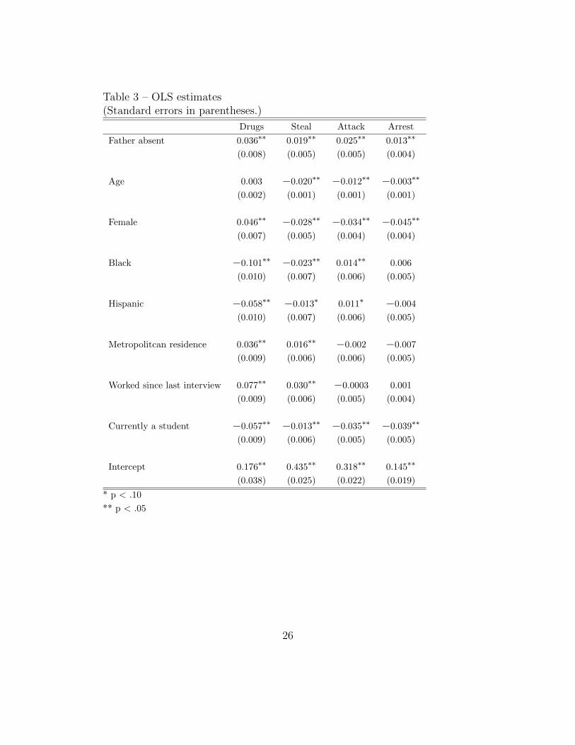
Table 3 – OLS estimates(Standard errors in parentheses.)

Drugs Steal Attack Arrest

Father absent 0.036∗∗ 0.019∗∗ 0.025∗∗ 0.013∗∗

(0.008) (0.005) (0.005) (0.004)

Age 0.003 −0.020∗∗ −0.012∗∗ −0.003∗∗

(0.002) (0.001) (0.001) (0.001)

Female 0.046∗∗ −0.028∗∗ −0.034∗∗ −0.045∗∗

(0.007) (0.005) (0.004) (0.004)

Black −0.101∗∗ −0.023∗∗ 0.014∗∗ 0.006

(0.010) (0.007) (0.006) (0.005)

Hispanic −0.058∗∗ −0.013∗ 0.011∗ −0.004

(0.010) (0.007) (0.006) (0.005)

Metropolitcan residence 0.036∗∗ 0.016∗∗ −0.002 −0.007

(0.009) (0.006) (0.006) (0.005)

Worked since last interview 0.077∗∗ 0.030∗∗ −0.0003 0.001

(0.009) (0.006) (0.005) (0.004)

Currently a student −0.057∗∗ −0.013∗∗ −0.035∗∗ −0.039∗∗

(0.009) (0.006) (0.005) (0.005)

Intercept 0.176∗∗ 0.435∗∗ 0.318∗∗ 0.145∗∗

(0.038) (0.025) (0.022) (0.019)

* p < .10

** p < .05

26

Table 4 – Fixed effects regression estimates(Standard errors in parentheses.)

Drugs Steal Attack Arrest

Father absent −0.036∗ 0.012 0.003 −0.024∗∗

(0.019) (0.015) (0.013) (0.012)

Age 0.013∗∗ −0.021∗∗ −0.011∗∗ 0.001

(0.002) (0.002) (0.001) (0.001)

Female − − − −

Black − − − −

Hispanic − − − −

Metropolitcan residence 0.020 0.018 −0.028 0.015

(0.032) (0.026) (0.022) (0.020)

Worked since last interview 0.047∗∗ 0.010 0.0003 0.002

(0.008) (0.006) (0.006) (0.005)

Currently a student 0.021∗∗ 0.008 0.011∗ −0.001

(0.009) (0.007) (0.006) (0.006)

Intercept −0.070 0.434∗∗ 0.273∗∗ 0.028

(0.047) (0.037) (0.032) (0.029)

* p < .10

** p < .05

27

Table 5 – Dynamic estimates(Standard errors in parentheses.)

Drugs Steal Attack Arrest

Father absent 0.016∗∗ 0.013∗∗ 0.014∗∗ 0.008∗

(0.007) (0.005) (0.005) (0.004)

Lagged dependent variable 0.536∗∗ 0.261∗∗ 0.229∗∗ 0.173∗∗

(0.008) (0.008) (0.008) (0.009)

Age −0.007∗∗ −0.013∗∗ −0.008∗∗ −0.003∗∗

(0.002) (0.001) (0.001) (0.001)

Female −0.028∗∗ −0.020∗∗ −0.027∗∗ −0.037∗∗

(0.007) (0.005) (0.004) (0.004)

Black −0.042∗∗ −0.016∗∗ −0.010∗ 0.004

(0.010) (0.007) (0.006) (0.005)

Hispanic −0.037∗∗ −0.013∗ 0.008 −0.005

(0.010) (0.007) (0.006) (0.006)

Metropolitcan residence 0.012 0.009 −0.004 −0.009∗

(0.009) (0.006) (0.006) (0.005)

Worked since last interview 0.046∗∗ 0.025∗∗ 0.002 −0.002

(0.008) (0.006) (0.005) (0.005)

Currently a student −0.011 −0.011∗ −0.023∗∗ −0.032∗∗

(0.008) (0.006) (0.005) (0.005)

Intercept 0.241∗∗ 0.288∗∗ 0.209∗∗ 0.142∗∗

(0.039) (0.028) (0.024) (0.022)

* p < .10

** p < .05

28

Table 6 – Dynamic fixed effects regression estimates(Means and standard deviations of posterior distributions.)

Drugs Steal Attack Arrest

Father absent −0.016 0.025 0.012 −0.023

(0.023) (0.017) (0.015) (0.014)

Lagged dependent variable 0.268∗∗ 0.123∗∗ 0.076∗∗ 0.116∗∗

(0.013) (0.011) (0.011) (0.013)

Age 0.002 −0.019∗∗ −0.008∗∗ 0.0003

(0.002) (0.002) (0.002) (0.002)

Female − − − −

Black − − − −

Hispanic − − − −

Metropolitcan residence 0.005 0.051∗ −0.012 0.002

(0.038) (0.028) (0.025) (0.023)

Worked since last interview 0.039∗∗ 0.017∗∗ 0.004 −0.001

(0.010) (0.007) (0.006) (0.006)

Currently a student 0.015 −0.001 0.008 −0.007

(0.010) (0.008) (0.007) (0.006)

* p < .10

** p < .05

29

Table 7 – Nonbiological male adult in household is not counted as “absent father”

Drugs Steal Attack Arrest

OLS

Father absent 0.020∗∗ 0.009 0.020∗∗ 0.009∗∗

(0.009) (0.006) (0.005) (0.004)

Fixed effects

Father absent −0.004 0.022∗ 0.007 −0.006

(0.016) (0.013) (0.011) (0.010)

Dynamic

Father absent 0.011 0.008 0.014∗∗ 0.005

(0.008) (0.006) (0.005) (0.005)

Dynamic fixed effects

Father absent 0.003 0.023 0.016 −0.023

(0.020) (0.015) (0.013) (0.014)

(These models include all controls listed in Tables 2-5.)

* p < .10

** p < .05

30

Table 8 – Add dummy for whether family income > 200% poverty line

Drugs Steal Attack Arrest

OLS

Father absent 0.038∗∗ 0.020∗∗ 0.025∗∗ 0.014∗∗

(0.009) (0.005) (0.005) (0.004)

Fixed effects

Father absent −0.035∗∗ 0.012 0.004 −0.023∗

(0.019) (0.015) (0.013) (0.012)

Dynamic

Father absent 0.018∗∗ 0.014∗∗ 0.014∗∗ 0.009∗∗

(0.008) (0.005) (0.005) (0.004)

Dynamic fixed effects

Father absent −0.014 0.026 0.012 −0.023

(0.023) (0.017) (0.016) (0.014)

(These models include all controls listed in Tables 2-5.)

* p < .10

** p < .05

31