The E ects of Gold Mining on Newborns’ Healthsantisap/Paper_mining_newborn_health.pdf · The E ects of Gold Mining on Newborns’ Health Mauricio Romero and Santiago Saavedra August

The Effects of Gold Mining on Newborns’ Health

Mauricio Romero and Santiago Saavedra∗

August 11, 2016

Abstract

Mining can propel economic growth, but often results in heavy metalreleases, that could negatively impact human health. Using a difference-in-differences strategy we estimate the impact of gold mining on the healthof newborns in Colombia. We find heterogeneous effects depending onwhere mothers are located with respect to a mine. Mothers living in thevicinity of a mine are positively affected experiencing a reduction of 0.51percentage points in the probability of having a child with low APGARscore at birth (from a basis of 4.5%). However, we find a negative effecton mothers living downstream from a mine, whose probability of havinga child with a low APGAR score at birth increases by 0.45 percentagepoints. We provide suggestive evidence that contaminated fish consump-tion in the first weeks of gestation is the mechanism behind our resultsusing an exogenous increase in fish consumption caused by a religiouscelebration.

1 Introduction

The surge in mineral prices over the last decade has propelled mining and eco-nomic growth in many low- and middle-income, mineral-rich countries (McMahon& Moreira, 2014). However, mining is usually accompanied by environmentaldegradation. The net impact of gold mining on human well-being is unclear, asmore income could potentially expand opportunities for people (e.g., access tomore and better food), while environmental degradation could negatively affecthuman health (e.g., respiratory infections and heavy metal poisoning).1 Addi-tionally, environmental degradation and its impact on human health could have

∗Romero: University of California - San Diego, e-mail contact: [email protected]. Saave-dra: Stanford University, e-mail contact: [email protected]. This study was carriedout with support from the Latin American and Caribbean Environmental Economics Pro-gram (LACEEP) grant IDEA-302. We are grateful to Prashant Bharadwaj, Pascaline Dupas,Thomas Ginn, LACEEP and seminar participants at PACDEV, Stanford and UC San Diego.Abraham Ibanez provided excellent research assistance.

1There is ample debate in the literature about the existence of the so-called environmentalKuznets curve, which predicts that the relationship between pollution and income has an

1

[email protected]

[email protected]

a detrimental effect on future income growth by reducing human capital. Inparticular, if newborns are negatively affected by environmental degradation,this could lead to lower future productivity as in-utero insults, birth outcomes,and early-life shocks have been shown to have long-term negative impacts oneducational attainment (e.g, see Almond (2006)), learning outcomes (e.g., seeBharadwaj, Løken, and Neilson (2013)), cognitive ability (e.g., see Almond andCurrie (2011)) and wages (e.g., see Black, Devereux, and Salvanes (2007)).

In this article, we study the effect of gold mining on newborns’ health in Colom-bia. Although gold mining provided $ 100 million (USD) in royalties in 2012, itoften results in the release of heavy metals (mercury in particular) that affectthe health of the surrounding population and especially infant brain develop-ment.2 In fact, recent legislation to control and regulate the use of mercury(with an explicit goal to phase-out its use in mining by 2018) was set in place to“protect human health and preserve natural resources” (Congreso de la Repub-lica, 2013). It is know that the main channel of mercury exposure is through fishconsumption. However, there is scant evidence on the magnitude of the effect ofmercury on surrounding populations, and whether the benefits of mining couldcompensate for any damage.

Our identification strategy is a difference-in-differences style estimator that com-pares births near mines with those far from them, before and after mining ac-tivity begins. The main dependent variable is whether the newborn has a lowAPGAR (Appearance, Pulse, Grimace, Activity and Respiration) score, whichcaptures the presence of possible brain damage (Moster, Lie, Irgens, Bjerkedal,& Markestad, 2001) and is a significant predictor of health, cognitive ability,and behavioral problems later in life (Almond, Chay, & Lee, 2005). We use arich data set with all births between 2001 and 2012, and administrative recordson the location, shape and boundaries of the mines.

We find heterogeneous effects depending on where the mothers are located withrespect to a mine. Babies born to mothers living near a mine are positively af-fected by mining activities and experience a reduction of 0.51 percentage pointsin the probability of having low APGAR score (from a basis of 4.5%). However,we find a negative effect on mothers living in municipalities located downstreamfrom a mine, whose probability of having a child with a low APGAR score atbirth increases by 0.45 percentage points.

The toxicology literature points to fish as the main channel of mercury expo-

inverted U shape, reflecting that pollution initially rises along with income but eventuallyreaches a turning point and starts to decline. However, the general consensus is that growthis accompanied by environmental degradation in developing countries. For a recent review ofthe literature on the environmental Kuznets curve see Carson (2010) and Harbaugh, Levinson,and Wilson (2002).

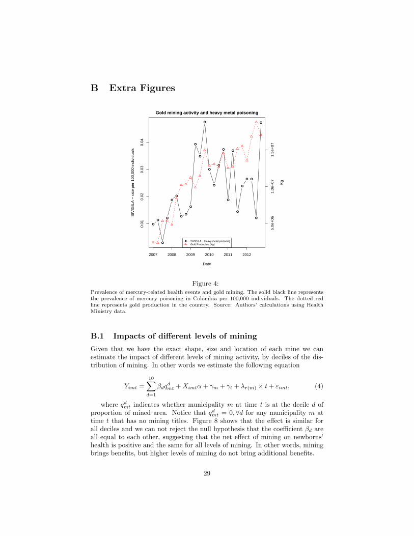
2The recent surge in gold mining has been accompanied by an increase in heavy metalpoisoning (see Figure 4 in Appendix B).

2

sure to humans. Thus, we provide suggestive evidence that contaminated-fishconsumption is the mechanism behind our results. We do this by studying anexogenous increase in fish consumption during pregnancy caused by Holy Week,a religious celebration during which fish consumption rises throughout the coun-try. An overlap of Holy Week with the first trimester of gestation increases thelikelihood of low APGAR at birth. We provide a number of robustness checks.In particular we show that our treatment effects decrease as we move away fromthe source of treatment (i.e., the mine or the river) and show that using theinternational gold price as an additional source of variation provides similar re-sults.

We contribute to the growing body of literature on the effects and externalitiesof mining, and specifically to the literature on mining in developing countriesand its effect on health outcomes. Although there has been an active literatureon the health effects of pollution, most of it has been using developed countries’data (Greenstone & Jack, 2015). Previous studies have found that mining hasnegative effects on the environment and agricultural productivity (McMahon &Remy, 2001; Aragon & Rud, 2015), while others have found positive incomeeffects on local communities (Aragon & Rud, 2013; von der Goltz & Barnwal,2014). The indirect effect of mining on human health has rarely been consideredin the literature; with the exception of von der Goltz and Barnwal (2014) andTolonen (2015). An advantage of our data is that we have the exact shape of themine, while von der Goltz and Barnwal (2014) and Tolonen (2015) only have onecoordinate point to identify the location of the mines. We show that our mainresults are similar whether we use all the information on the mines’ shape, orjust its centroid. However, the heterogeneity with respect to the distance fromthe mine is different if we use only one point to identify the location instead ofthe exact shape of the mine. Finally, although previous studies have use otherreligious celebration (e.g., Ramadan) as a source of exogenous variation (e.g.,see Almond and Mazumder (2011) and Schofield (2015)), we are not aware ofany study that exploits Holy Week as a source of variation.

The rest of the article is organized as follows: Section 2 contains a review of theeffects of mercury on human health and Section 3 describes the context of min-ing in Colombia and the data. Section 4 presents the identification strategy andthe construction of the variables. Section 5 presents the main results, while Sec-tion 6 presents robustness checks. The final section contains concluding remarksand a discussion of avenues for further research.

2 Mercury and human health

A number of papers have identified a strong correlation between mining andadverse environmental and health outcomes. For example, Swenson, Carter,Domec, and Delgado (2011) find that increases in gold prices have boostedsmall-scale gold mining in Peru and led to increased deforestation in the Ama-

3

zon jungle. Hilson (2002) finds that small-scale gold mining in Ghana led tosocioeconomic growth but also mercury pollution and land degradation. Moststudies linking health to mining also focus on correlation and, due to confound-ing effects, cannot imply causation (Fernandez-Navarro, Garcıa-Perez, Ramis,Boldo, & Lopez-Abente, 2012; Attfield & Kuempel, 2008; Chakraborti et al.,2013). The few papers that have attempted to tease out the causal componenthave focused on the effect of mining on agricultural productivity: Aragon andRud (2015) estimate that mining in Ghana reduced agricultural productivity innearby areas by almost 40%; and on spillovers to non-mining activities Aragonand Rud (2013) find a positive effect of mining on real income for non-miningworkers in Peru. However, the extent to which mining affects health is stillunclear.

We are only aware of one article, by von der Goltz and Barnwal (2014), thatcredibly identifies the effect of mining on health. In their article, von der Goltzand Barnwal (2014) use mine locations (mine centroids) and the year a minestart operations to identify the effect of mines on wealth and health. They findthat communities near mines in Africa have higher asset wealth but also higherrates of anemia. Our study is similar in spirit, but differs in three important di-mensions. First, we have information on size and shape of the mines which allowus to calculate intensive margin effects (we find that there are none). Second,we study the impact of mining on cognitive development using as a proxy theAPGAR score at birth. Third, we are able to separate the effects of increasedincome and increased pollution by exploiting the fact that water pollution flowsdownriver, while the economic gains accrue to all surrounding areas.

2.1 Mercury and amalgamation in gold mining

Metallic mercury is used in mining for amalgamation, the process of separat-ing gold particles from other minerals (Mol, Ramlal, Lietar, & Verloo, 2001).For every kilogram of gold produced, on average 9 kilograms of mercury arereleased into the environment (Pfeiffer, Lacerda, Salomons, & Malm, 1993; daVeiga, 1997; Guiza & Aristizabal, 2013). Miners add mercury to silt in or-der to create an amalgam, a bond between mercury and gold. The remain-ing silt is then washed away. The amalgam is heated in smelters, where themercury evaporates and the gold nuggets are separated. 55% of the mercuryused enters the atmosphere, while 45% infiltrates bodies of water (Pfeiffer &de Lacerda, 1988). Aquatic microorganisms transform metallic mercury intomethyl-mercury (Morel, Kraepiel, & Amyot, 1998). The microorganisms areeaten by fish, and in turn humans are exposed to methyl-mercury by consum-ing contaminated fish (for a more detailed explanation see Mol et al. (2001)).In the U.S., the EPA limits for metallic mercury in drinking water and formethyl-mercury consumption are 0.002 mg/L and 0.1 µg/kg body weight/day,respectively. There is evidence that those limits are exceeded in Colombia nearmining areas (Guiza & Aristizabal, 2013; Olivero & Johnson, 2002).

4

Artisanal and small-scale gold mining is the largest contributor to atmosphericmercury emissions at 727 tons annually, or 35% of anthropogenic emissions. Inaddition, discharges into water bodies from small-scale mining are estimated at800 tons each year, representing 63% of anthropogenic releases (United NationsEnvironment Programme, 2013). Large-scale gold mining is classified as unin-tended mercury emission, because it is assumed that mercury is either capturedand stockpiled or sold for other uses. This sector accounts for 97 tones, or 5%of emissions. In short, the two main sources of human exposure to mercury arethrough methyl-mercury in fish and mercury vapor from smelters. In the datasection, to possibly account for the air channel, we use the proportion of areamined in the municipality and the proximity of the population to the mines.For the water channel we use exposure of the population to river pollution.

2.2 Health effects of mercury

Mercury is one of the top ten chemicals of major public health concern accordingto the World Health Organization (World Health Organization, 2013). Thereare five factors that determine the intensity of mercury health effects: the typeof mercury; the dose; duration of exposure; route of exposure; and the ageof the person (World Health Organization, 2013). An advantage of studyingthe health effects on newborns is that the age, type, duration, and route ofexposure are known. Dosage, on the other hand, depends on fish consumptionduring pregnancy, as well as to mercury levels (if any) in the fished consumed.

The medical literature consistently points out that exposure to methyl-mercuryin high doses can be fatal (Davidson, Myers, & Weiss, 2004), but there is noconsensus on how variation in the dosage affects health.3 Mercury is harmfulto the heart, kidneys, and central nervous system, with women and childrenbeing the most sensitive to its effects. There is evidence that the fetal brainis especially susceptible to damage from exposure to mercury (Davidson et al.(2004), Environmental Protection Agency (2013), Black, Butikofer, Devereux,and Salvanes (2013). Babies born to women poisoned with methyl-mercuryare more likely to develop cerebral palsy (Center for Disease Control, 2009), inturn a low APGAR score at birth is associated with an 81-fold increase in therisk of cerebral palsy (Moster et al., 2001). APGAR scores have been found tobe a significant predictor of health, cognitive ability, and behavioral problemslater in life, even after controlling for family background and low birth weight(Almond et al., 2005). We are not aware of literature discussing mercury effectson height, birth weight or length of gestation (the other newborn outcomes wehave information for).

3See Mergler et al. (2007) , Davidson et al. (2004), Counter and Buchanan (2004), andClarkson, Magos, and Myers (2003) for reviews of the literature.

5

3 Colombian context and data

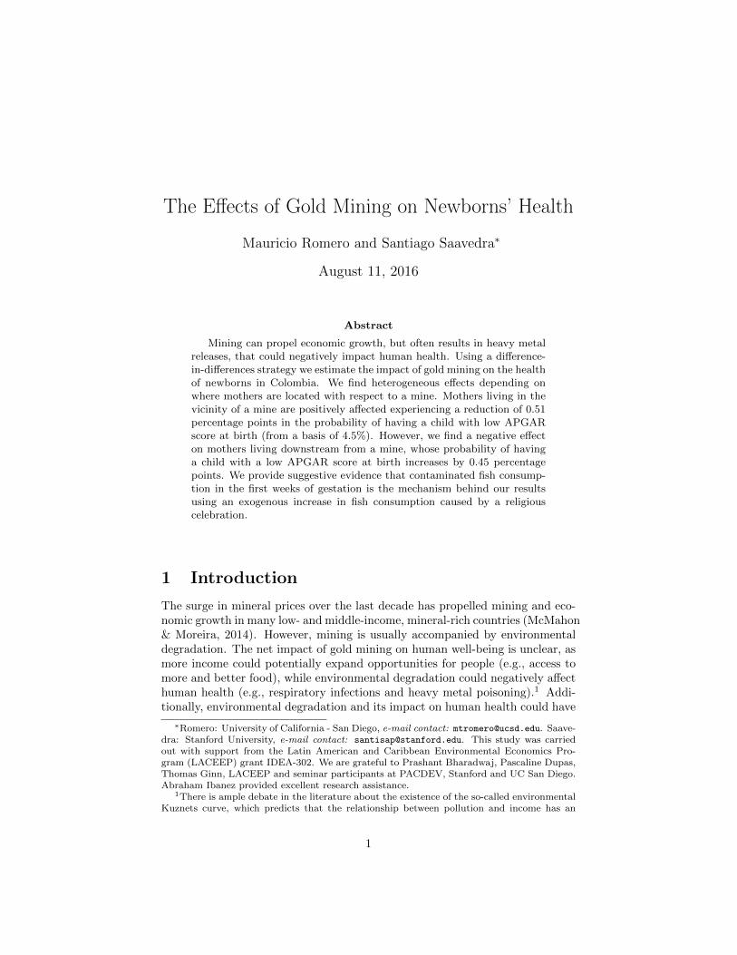
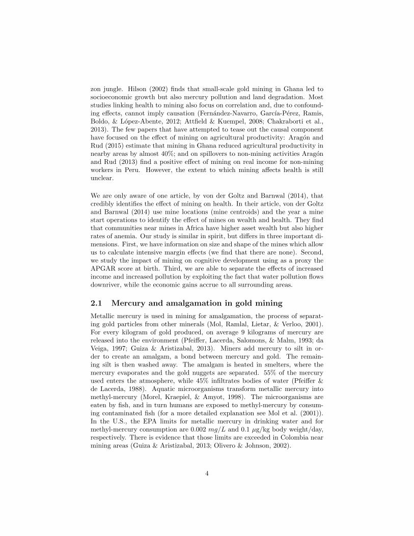
Colombia is currently experiencing a mining boom: gold extraction increasedby more than 180 % between 2004 and 2012 (see Figure 1).4 The nationalgovernment allocates mining permits allowing exploration in a given area.If acompany decides to exploit the resource, it has to apply for an extraction permitand environmental license.5

● ● ● ●● ● ● ●

● ● ● ●

●

●●

●

●

●

●

●

●

●

●

● ● ●

● ●

●

●

● ●

●

●

●

●

●●

●

●

●●

●●

●

●

●

●

●

●

●

●

2002 2004 2006 2008 2010 2012

5000

1000

015

000

Mining in terms of area and production

Date

Kg

050

0010

000

1500

020

000

Km

^2

● Production (Kg)Mined area (km^2)

Figure 1:The figure shows the evolution over time of gold production (in kilograms) and total minedarea (in square kilometers). Source: Ministerio de Minas y Energia de Colombia. Calculations:Authors.

Mining companies operating in Colombia have to pay royalties to the gov-ernment; the revenue is distributed among the central, and local governments.6

4Author calculations based on Government data from Mining Permits and Sistema deInformacion Minero Colombiano (SIMCO).

5In a previous version of this paper we considered the application for mining permits a goodproxy for mineral discovery that would lead to extraction of the mineral shortly thereafter,either legally or illegally. Now we use only information for when the title is actually in theextraction phase.

6The rate for gold mining in our period of study was 4% of production at market prices,except for non-artisan alluvial mining which had a rate of 6%. As of 2012, the central gov-ernment kept 7.5% of this revenue, 5% went to the state government, while the municipalitywas allocated 87%. The remaining 0.5% was distributed to municipalities with ports wherethe gold was exported.

6

Most of the revenue allocated to the local government must, by law, be used toimprove infant mortality, health access, education coverage, clean water accessand sanitation indicators.

3.1 Data on mining activity

Since there are no measurements of atmospheric or water-borne mercury levels,we approximate mercury use with gold extraction (by municipality productionand by area of the mine).7 Mining location and area are obtained from the min-ing permit database maintained by the nongovernmental organization TierraMinada based on official government records from the Catastro Minero Colom-biano.8

We combine this information with gold production at the municipality levelpublished by the government agency SIMCO (Sistema de Informacion MineroColombiano), available since 2001.9. However, we focus on mining area, as op-posed to production due to several reasons. First, production is only releasedat the municipality level. We were denied access to production data at themine level by the Ministry of Mining due to confidentiality issues. Thus, fromthe production data we are unable to asses proximity from an active mine, orthe nearest river from an active mine. Second, there are several inconsistenciesin the production data: of the 7,7134 municipality-month observations withpositive production, only 56% had at least one active mining permit.10 Therehave been reports of collusion between illegal miners and government officials innon-mining municipalities: officials report production as a means to “laundry”illegal gold, which in turn increases royalties revenues for the municipality (ElEspectador, 2015b, 2015a). Finally, mining permits are a good proxy for min-eral discovery that would lead to extraction of the mineral shortly thereafter,either legally or illegally. Therefore, mining permits are better proxy for overallmining activity than reported production, as the latter might have under orover reporting due to illegal and artisan mining.

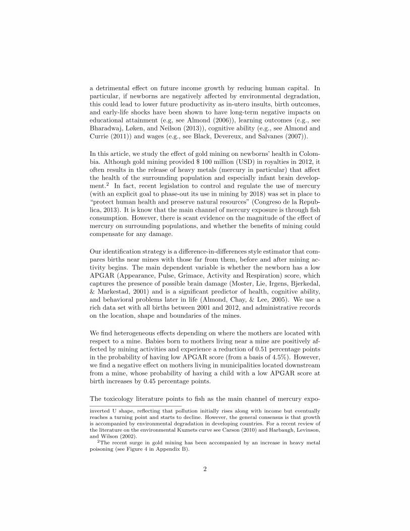
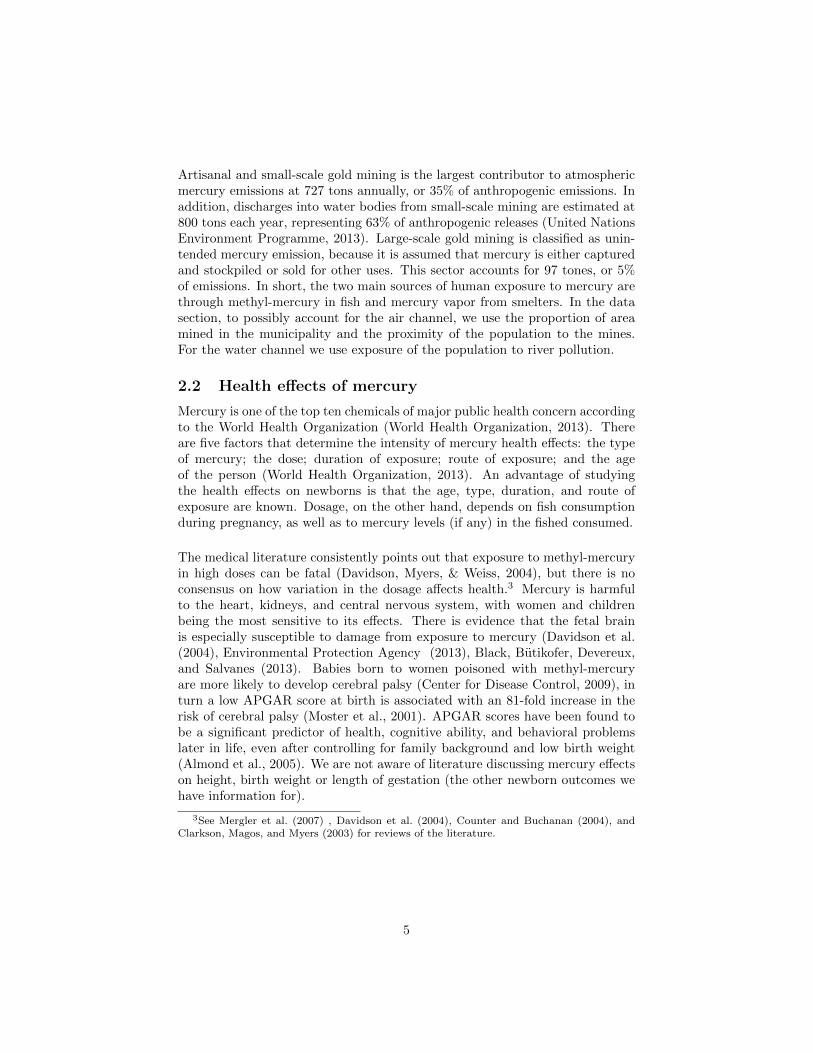
The proportion of municipalities with gold permits has increased dramatically,while the increase in municipalities with gold production has been more modest(see Figure 2). Although part of this discrepancy between municipalities with

7Almost all (99.7%) of the municipality-month mercury observations for 2006-2012 aremissing in the National Health Institute- Information System of Monitoring of Water forHuman Consumption-SIVICAP http://www.ins.gov.co/sivicap/Paginas/sivicap.aspx

8The full data set can be downloaded from https://sites.google.com/site/

tierraminada/9From 2001 to 2003 the data was released annually, but since 2004 it has been published

on a quarterly basis.10This is an upper bound, as we do not have data on environmental licenses, which are

necessary to extract gold legally.

7

http://www.ins.gov.co/sivicap/Paginas/sivicap.aspx

https://sites.google.com/site/tierraminada/

https://sites.google.com/site/tierraminada/

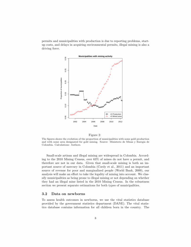
permits and municipalities with production is due to reporting problems, start-up costs, and delays in acquiring environmental permits, illegal mining is also adriving force.

● ● ● ● ● ● ● ●

● ● ● ●

● ● ●

●●

●

●

●● ● ●

● ●● ● ● ● ●

●●

● ● ●●

● ●● ● ●

●●

●●

● ● ● ● ●

●●

2002 2004 2006 2008 2010 2012

0.05

0.10

0.15

0.20

0.25

0.30

Municipalities with mining activity

Date

Pro

port

ion

of m

unic

ipal

ities

● >0 Production>0 Mined area

Figure 2:The figures shows the evolution of the proportion of municipalities with some gold productionand with some area designated for gold mining. Source: Ministerio de Minas y Energia deColombia. Calculations: Authors.

Small-scale artisan and illegal mining are widespread in Colombia. Accord-ing to the 2010 Mining Census, over 63% of mines do not have a permit, andtherefore are not in our data. Given that small-scale mining is both an im-portant source of mercury in Colombia (Cordy et al., 2011) and an importantsource of revenue for poor and marginalized people (World Bank, 2009), ouranalysis will make an effort to take the legality of mining into account. We clas-sify municipalities as being prone to illegal mining or not depending on whetherthey had an illegal mine listed in the 2010 Mining Census. In the robustnesssection we present separate estimations for both types of municipalities.

3.2 Data on newborns

To assess health outcomes in newborns, we use the vital statistics databaseprovided by the government statistics department (DANE). The vital statis-tics database contains information for all children born in the country. The

8

information include APGAR score11, weight, height, length of the gestation,hospital of birth and municipality where the mother lives. However, since AP-GAR is a subjective measure, we use an indicator for whether the newborn hada score below 7 as is common practice in the literature (Ehrenstein, 2009).12.We standardize height and weight using information from the World HealthOrganization (2006). The vital statistics database also include information onthe mother such as age, education, marital status, and whether she attendedprenatal appointments or not.

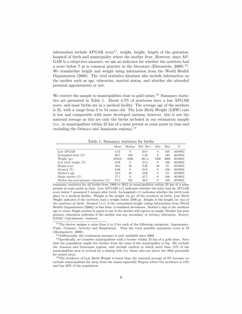
We restrict the sample to municipalities close to gold mines.13 Summary statis-tics are presented in Table 1. About 4.5% of newborns have a low APGARscore, and most births are in a medical facility. The average age of the mothersis 25, with a range from 9 to 54 years old. The Low Birth Weight (LBW) rateis low and comparable with more developed nations; however, this is not thenational average as this are only the births included in our estimation sample(i.e., in municipalities within 25 km of a mine permit at some point in time andexcluding the Orinoco and Amazonia regions).14

Table 1: Summary statistics for birthsMean Median Std. Dev. Min Max N

Low APGAR 4.55 0 20.8 0 100 4019952In-hospital birth (%) 99.7 100 5.46 0 100 4019952Weight (gr) 3163.6 3200 461.4 1500 4300 4019952Low birth weight (%) 6.88 0 25.3 0 100 4019952Height (cm) 49.6 50 2.35 40 55 4019952Stunted (%) 6.60 0 24.8 0 100 4019952Mother’s age 24.8 24 6.60 9 54 4019952Single mother (%) 17.1 0 37.7 0 100 4019952Mother has post-primary education (%) 67.5 100 46.8 0 100 4019952

Summary statistics for all births from 1999 to 2012 in municipalities within 25 km of a minepermit at some point in time. Low APGAR(=1) indicates whether the baby had an APGARscore below 7 measured 1 minute after birth. In-hospital(=1) indicates whether the birth tookplace in a medical facility. Weight is the weight (in gr) of the newborn at birth, Low BirthWeght indicates if the newborn had a weight below 2500 gr. Height is the height (in cm) ofthe newborn at birth. Stunted (=1) if the normalized height (using information from WorldHealth Organization (2006)) is less than -2 standard deviations. Mother’s Age is the mothersage in years; Single mother is equal to one if the mother self reports as single; Mother has postprimary education indicates if the mother has any secondary or tertiary education. Source:DANE. Calculations: Authors.

11The doctor assigns a value from 0 to 2 for each of the following categories: Appearance,Pulse, Grimace, Activity and Respiration. Thus the total possible maximum score is 10(Montgomery, 2000).

12Additionally, the continuous measure is only available since 2008.13Specifically, we consider municipalities with a border within 25 km of a gold mine. Note

that the population might live further from the mine if the municipality is big. We excludethe Amazon and Orinoquia regions, and exclude outliers in which more than 15% of themunicipalities area is covered by a mining title (i.e, those who are above the 99th percentilefor mined area).

14The incidence of Low Birth Weight is lower than the national average of 9% because weexclude municipalities far away from the mines especially Bogota where the incidence is 13%and has 20% of the population.

9

4 Identification strategies

4.1 Spatial exposure to mining

Our identification strategy is a difference-in-differences that compares birthsnear mines with those far from them, before and after mining begins. In orderto do this, we must identify births near mines, as well as births downstream frommines. To do the former, we create 5, 10 and 20-kilometer buffers around eachmine, and calculate for each municipality the average mined area per capita ina given period (NearMiningmt).

15

To identify births downstream from mines, we would ideally classify eachmunicipality as being upstream or downstream from a mine. Unfortunatelythis is not feasible as rivers often enter and exit municipalities several times;therefore, we estimate the exposure to upstream mining in each municipalitythrough various steps. First, using a data set of all rivers in Colombia weidentify the closest river to each mine (usually running through the mine16).For each river segment we calculate the total area from active mines closest toit; and aggregate the total area upstream up to 25 km.17. In short, the totalexposure in river segment j is estimated by:

River Exposurej =∑i∈Uj

1D(i,j)<25Areai,

where Uj is the set of river segments located upstream from segment j, D(i, j)is the distance (following the course of the river) from segment j to segment i inkilometers, Areai is the total area of active mining titles to which river section iis the closest river to them. The pollution value for segment j therefore dependson how many mines pollute segments upstream, and the size of such mines. Wethen create 5, 10 and 20-kilometer buffers along the river and calculate the theaverage area mined upstream per capita in a given period for each municipality(UpstreamMiningmt).

18. These calculations are done using geographical infor-mation systems (GIS) in R.

We use this measure of “upstream mining” to identify the effect of pollution fromgold mining on health. However, there is an important underlying assumptionin this approach: pollutants that are discharged into the river do not affect the

15More explicitly, for buffer we create a raster with the mined area and multiply it withthe population raster of each municipality. We then sum this over each municipality, andcalculate the value per capita.

16A river runs through the entitled area of 48% of the mines. The average distance fromthe mines to a river is 0.8 km, and the furthest is 5 km (the presence of small creeks is notconsidered, as they do not appear in our river’s database).

17Bose-O’Reilly et al. (2010) finds that fish more than 25 km downstream from a mine inTanzania have a low concentration of mercury. The actual concentration of mercury dependson the type of soil, water flow, and other variables that are not available.

18More explicitly, for buffer we create a raster with the upstream mined area and multiplyit with the population raster of each municipality. We then sum this over each municipality,and calculate the value per capita.

10

population living upstream. A necessary condition for this assumption is thatfish eaten by humans are caught locally and do not travel upstream.

The specific regression we estimate is:

Yimt = β1NearMiningmt + β2UpstreamMiningmt

+Xiα+ γm + γt + λs(m) × t+ εimt, (1)

where NearMiningmt is a measure of exposure to mines nearby (in all direc-tions) constructed as explained previously.UpstreamMiningmt is a measure ofexposure to pollution discharged upstream from municipality m at time t con-structed as explained above. This variable measures the area (in km2) minedupstream to which the average inhabitant in municipality m at time t is ex-posed. Notice that upstream here is any mine that is less than 25 kilometersaway from the municipality (along the river) and an individual is exposed if heis within the buffer of the river. γm are municipality fixed effects to controlfor initial differences in mining municipalities (see Ibanez and Laverde (2014)).γt are year and week of the year fixed effects and λs(m) × t are state dummyvariables interacted with a time trend to allow for differential time trends foreach state. The coefficients of interest are β1 and β2. β1 captures the net (in-come and pollution) effect of mining on nearby communities and β2 allows usto capture the negative externalities (if any) that mining has on downstreamcommunities.

Measurement error is a problem for our measures of mining activity due toillegal mining and differences between the area licensed and the actual area ex-ploited. Additionally, although our spatial calculations try to estimate in thebest possible manner exposure to gold mining, they are far from perfect: a)mines can potentially discharge their waste in other rivers; b) we do not havethe exact location of each mother’s dwelling and must therefore rely on munic-ipality averages. For this reasons our main specification uses dummy variablesthat indicate whether the municipalities had any exposure (NearMiningmt > 0and UpstreamMiningmt > 0) . This is the strategy used in most articles study-ing the effects of mining.19

We test whether there is any difference in the trends of newborns before andafter mining begins in a municipality. Given that we can not observe newbornsbefore birth, we collapse the data at the municipality-quarter level and estimatethe following regression:

Ymt =

6∑j=−6

βτ1τm+j=t +

6∑j=−6

απ1πm+j=t + γm + γt + λr(m) × t+ εmt, (2)

where τm is the quarter in which municipality m has a mine nearby for the firsttime and πm is the quarter in which municipality m has a mine upstream for the

19For example, see von der Goltz and Barnwal (2014) and Santos (2014).

11

first time. Therefore 1τm+j=t and 1πm+j=t are indicator variables that are equalto one if year t is j years before/after “near mining” and “upstream mining”begins. Notice that for municipalities that have no exposure these dummies areequal to zero. We plot β−6, ..., β6 to see how the Ymt changes at the municipalitylevel before and after mining nearby begins. Similarly, we plot α−6, ..., α6 to seehow the Ymt changes at the municipality level before and after upstream miningbegins.

4.2 Holy Week

Colombia is predominantly a Catholic country, with over 75% of the populationdeclaring themselves as Catholic.20 Holy Week is one of the major Catholictraditions, and both Maundy Thursday and Good Friday are national holidays.Fish consumption increases during Holy Week by 60% (El Colombiano, 2014),and, together with the increase in fish consumption during Lent, this representsan approximate 5% increase in fish consumption during the gestation period ofa baby.21 We use this exogenous increase in fish consumption to estimate thetreatment effect of methyl-mercury exposure on health. An advantage of usingHoly Week is that its exact date varies from year to year22 allowing us to par-tially separate the effect of mercury exposure from seasonal effects. Specifically,we estimate the following equation:

Yimt = β1Goldmt + β2Holy weeki + β3Goldmt ×Holy weeki+Xiα+ γm + γt + λs(m) × t+ εimt, (3)

where Holy weeki is a dummy variable that indicates whether individual i’sgestational period overlaps with Holy Week and γm are municipality fixed ef-fects. Note that γt includes week fixed effects so we are not capturing seasonaleffects. The coefficient of interest is β3, which captures the differential effectthat eating more fish during gestation has on newborns in areas with gold pro-duction or affected by pollution from gold mines, while β2 measures the effectof the gestational period overlapping with Holy Week (e.g., through additionalfish consumption or behavioral change for religious reason) and β1 captures thenet effect of gold mining on newborns’ health.

There are however three main problems with this exercise. First, we are onlyable to partially separate any seasonal effects as Holy Week only varies withina 34-day period. Second, nearly 75% of newborn have a gestational periodthat overlaps with Holy Week at some point, and the exogenous increase in fish

20According to Latinbarometro 2011. The number is closer to 80% according to the PewResearch: Religion & Public Life Project 2012.

21From a survey of fish vendors in 14 municipalities, we found that prices during Holy Weekare the same as the rest of the year for 88% of 171 species-market observations and on averageprices increase by 3%. Consequently, we do not expect differentiated effects by income.

22Since 525 A.D., the last day of Holy Week (Easter) has been established as the Sundayafter the first full moon following the March equinox. Therefore, the holiday varies from yearto year, but it is always between March 22 and April 25.

12

consumption only lasts for one week of the entire gestational period. Third, fishis often not eaten where it is caught. On a survey we did in 2014 we foundthat 59% of species-markets observations come from intermediaries from otherunknown municipalities. All these problems make this empirical exercise low-powered, but we include it since the results suggest that increased consumptionof fish from polluted rivers has negative effects on health.

5 Results

5.1 Spatial exposure

The results from estimating the effect of mining on nearby and downstreammunicipalities (equation 1) are presented in Table 2. Panel A shows that al-though the net effect of gold mining activity on the APGAR score of newbornsin surrounding populations is positive, the effect on downstream populations isnegative. We find that the likelihood of having low APGAR births decreasesfor mothers living within 20 km from a mine by 0.51 percentage points (PanelA, Column 1) (a reduction of 11%), while the likelihood increases for mothersliving downstream from a mine by 0.45 percentage points (an increase of 9.8%).These results have several implications: First, the costs and benefits of miningare not uniformly distributed across space; second, the costs of mining for thewhole country could potentially be greater than the benefits for the mining mu-nicipalities. In particular, in our sample, 69.90% take place downstream froman active mine, while 58.98% take place in the vicinity of a mine23. Figures 5-6in Appendix B show a detail distribution of births and municipalities near anddownstream from mines across time. Panel B shows that these effects decaywith distance (as expected), but are persistent up to 20 kilometers. Living neara mine has no effect on Low Birth Weight or Stunting, while having mining ac-tivity upstream seems to increase the likelihood of stunting by 0.29 percentagepoints. We are not aware of any study relating mercury or mining to stunnedbirth and the effect does not decay with distance (it seems to increase), there-fore we do not place much emphasis on this result and attribute it to samplingvariation.

2356.7% of births take place simultaneously downstream from a mine and in the vicinity ofa mine.

13

Table 2: Effect of proximity and river pollution exposure on birth outcomes

Dependent variable:Low APGAR Low Birth Weight Stunting

Panel A: Exposure up to 20 KMNear mining 20 km > 0 -0.51* -0.041 0.058

(0.27) (0.081) (0.12)Mining upstream 20 km > 0 0.45*** -0.0026 0.29***

(0.15) (0.080) (0.10)N. of obs. 4019952 4019952 4019952Municipalities 642 642 642Mean of Dep. Var. 4.55 6.88 6.60R2 0.017 0.0041 0.0049

Panel B: Exposure by distanceNear mining 5 km > 0 -0.90** 0.040 -0.10

(0.37) (0.12) (0.19)Near mining 5-10 km > 0 -0.61** -0.11 0.047

(0.28) (0.11) (0.17)Near mining 10-20 km > 0 -0.42* -0.0075 0.15

(0.25) (0.085) (0.13)Mining upstream 5 km > 0 0.62** -0.015 0.33*

(0.28) (0.13) (0.18)Mining upstream 5-10 km > 0 0.59** -0.15 0.17

(0.28) (0.13) (0.19)Mining upstream 10-20 km > 0 0.40** 0.030 0.32***


All regressions include municipality fixed effects, time fixed effects, individual controls andregional trends. Time fixed effects are year and week fixed effects. Individual controls in-clude mother’s age, an indicator for single mother and an indicator for whether the motherhas any post-primary education. The regional trends allow for a trend for each geographicregion (Pacific, Andean and Caribbean). Standard errors, clustered by municipalities, are inparentheses. ∗ p < 0.10, ∗∗ p < 0.05, ∗∗∗ p < 0.01

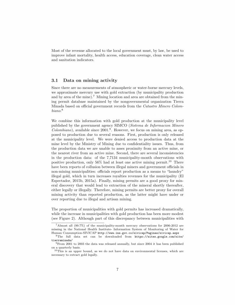
The main threat to identification is that the parallel trends assumption isnot met; namely, that municipalities exposed to mining experience a differentialtrend in the likelihood of Low APGAR in births prior to the exposure comparedto other municipalities. Figure 3 shows the result from estimating equation 2.As can be seen, there is a structural change in the likelihood of Low APGARbetween three and two years prior to the proximity exposure (matching the re-sults from the previous section). As explained before, this is somewhat expectedsince prior exploration of the area brings employment and income to the region.However, notice that the effect of river exposure only appears the year that theactual mining title is given. This results matches our prior intuition since riversshould carry pollution only after mining begins.

14

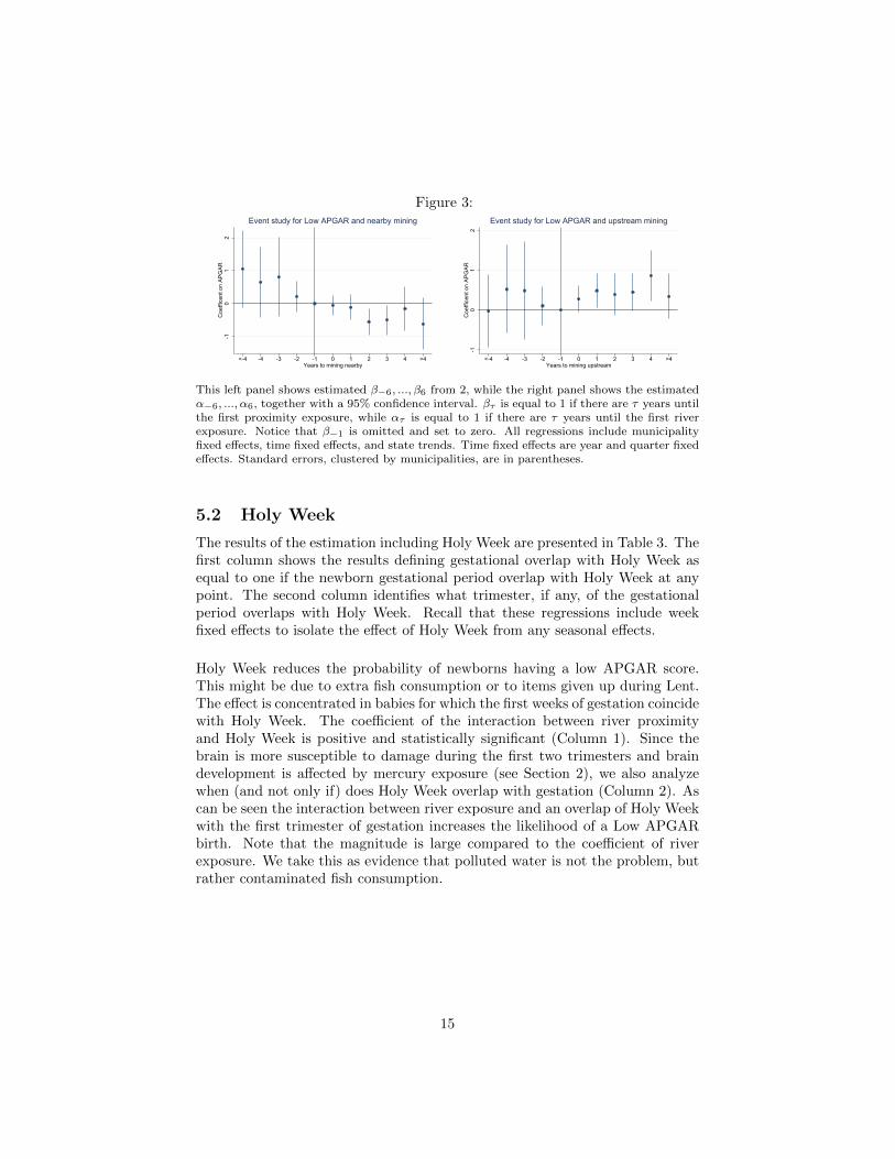
Figure 3:

-10

12

Coe

ffice

nt o

n AP

GAR

<-4 -4 -3 -2 -1 0 1 2 3 4 >4Years to mining nearby

Event study for Low APGAR and nearby mining

-10

12

Coe

ffice

nt o

n AP

GAR

<-4 -4 -3 -2 -1 0 1 2 3 4 >4Years to mining upstream

Event study for Low APGAR and upstream mining

This left panel shows estimated β−6, ..., β6 from 2, while the right panel shows the estimatedα−6, ..., α6, together with a 95% confidence interval. βτ is equal to 1 if there are τ years untilthe first proximity exposure, while ατ is equal to 1 if there are τ years until the first riverexposure. Notice that β−1 is omitted and set to zero. All regressions include municipalityfixed effects, time fixed effects, and state trends. Time fixed effects are year and quarter fixedeffects. Standard errors, clustered by municipalities, are in parentheses.

5.2 Holy Week

The results of the estimation including Holy Week are presented in Table 3. Thefirst column shows the results defining gestational overlap with Holy Week asequal to one if the newborn gestational period overlap with Holy Week at anypoint. The second column identifies what trimester, if any, of the gestationalperiod overlaps with Holy Week. Recall that these regressions include weekfixed effects to isolate the effect of Holy Week from any seasonal effects.

Holy Week reduces the probability of newborns having a low APGAR score.This might be due to extra fish consumption or to items given up during Lent.The effect is concentrated in babies for which the first weeks of gestation coincidewith Holy Week. The coefficient of the interaction between river proximityand Holy Week is positive and statistically significant (Column 1). Since thebrain is more susceptible to damage during the first two trimesters and braindevelopment is affected by mercury exposure (see Section 2), we also analyzewhen (and not only if) does Holy Week overlap with gestation (Column 2). Ascan be seen the interaction between river exposure and an overlap of Holy Weekwith the first trimester of gestation increases the likelihood of a Low APGARbirth. Note that the magnitude is large compared to the coefficient of riverexposure. We take this as evidence that polluted water is not the problem, butrather contaminated fish consumption.

15

Table 3: Increased mercury exposure in-utero due to Holy Week

Dependent variable: Low APGAR(1) (2)

Holy Week -0.79***(0.10)

Near mining 20 km > 0 -0.36 -0.36(0.31) (0.31)

Mining upstream 20 km > 0 0.33* 0.33*(0.18) (0.18)

Near mining × Holy Week -0.15(0.095)

Upstream mining × Holy Week 0.20*(0.11)

Holyweek 1st trimester -0.30***(0.11)

Holyweek 2nd trimester -0.55***(0.13)

Holyweek 3rd trimester -1.04***(0.13)

Near mining × Holy Week 1st Trim -0.12(0.11)

Near mining × Holy Week 2nd Trim -0.16(0.11)

Near mining × Holy Week 3rd Trim -0.18(0.11)

Upstream mining × Holy Week 1st Trim 0.28**(0.13)

Upstream mining × Holy Week 2nd Trim 0.22(0.14)

Upstream mining × Holy Week 3rd Trim 0.068(0.12)

N. of obs. 3567788 3567788Mean of Dep. Var. 4.48 4.48R2 0.017 0.017

All regressions include municipality fixed effects, time fixed effects, individual controls andstate trends. Time fixed effects are year and week of the year fixed effects. Individual con-trols include mother’s age, an indicator for single mother and an indicator for whether themother has any post-primary education. Standard errors, clustered by municipalities, are inparentheses. ∗ p < 0.10, ∗∗ p < 0.05, ∗∗∗ p < 0.01

16

6 Robustness checks

In this section we check the robustness of our results to using other measures ofmining activity; interacting our measures of mining with the price of gold; theeffect of gold mining on fiscal measures; possible changes on mother character-istics due to mining; and illegal mining.

6.1 Other measures of mining activity

In order to asses the robustness of our results to the spatial measures we use,we repeat our main regressions using simple measures of mining activity. Themeasures we use are the proportion of the area of the municipality that is mined,the accumulated production by municipality and indicators of these variablesbeing positive. The results are presented in table 4 on the Appendix. We findthat having mining area in the municipality reduces the probability of a babyborn with low APGAR by 0.58 percentage points (column 1 Panel B). This issimilar in magnitude to the coefficient of 0.51 when using our dummy of “nearmining”. However for accumulated production the sign is not stable when usingthe continuous measure or the dummy. This is probably due to the reportingproblems mentioned in Section 3.1.

6.2 Price of gold

The income effect of gold mining depends on the price of gold via more incomefor the same quantity extracted and also because a higher price encourages moreextraction. We present the results of interacting the mining variables with theprice of gold in Table 5. Column 1 repeats the main results of table 2, whilecolumn 2 presents the analogous regressions with the mining variables interactedwith the price of gold. This exercise shows, as before, that the net effect of goldmining is positive. In places with any mining (i.e., mining area > 0) an increaseof 10 dollars in the price of gold (per troy ounce) is associated with a 0.01percentage-point improvement in the APGAR scores of newborns.

6.3 Fiscal effect on municipalities

We do not have household level data to analyze assets or consumption of house-holds, but we do have information on the municipality budgets. Table 6 presentsthe effect of gold production in municipality budget and royalties. There is nosignificative effect of our mining measure on the fiscal variables of the munici-pality.

6.4 Birth and mother characteristics

We estimate the analogous of equation 1 using as the dependent variable differ-ent municipality and mother characteristics to see if there is any selection in oursample. In particular, at the municipality level we check whether the number

17

of births, the perinatal mortality, or the infant mortality change when exposureto mining changes. At the individual level we check whether the number of pre-natal checkups, the likelihood of a premature birth, the likelihood of in-hospitalbirth, the likelihood that the mother has subsidize health care and the mother’sage, marital status and education change when exposure to mining changes.

Table 7 shows that proximity to a gold mine (Column 1) increases the like-lihood of in-hospital births and more than four pre-natal checkups and reducesthe likelihood of premature birth. These results can be taken as signs of se-lection into our sample, but also as evidence of the mechanisms behind the“positive” effect of mining on APGAR scores. Specifically, as mining royaltiesmust be partially spend on health and to reduce infant mortality, mining in-creases the availability of health care (and therefore increases the likelihood ofin-hospital births and at least 4 pre-natal checkups) and reduces perinatal andinfant mortality, as well as premature births. The results in Column 2 showthat river exposure has no impact on the number of births, their characteristicsor mother characteristics. The point estimates are consistently close to zero andstatistically insignificant. We take this as evidence that there is no sorting dueto upstream pollution or proximity to mines, and therefore that our estimatesare free of sample bias.

6.5 Illegal mining

Table 8 provides the results of estimating equation 1 separately for municipal-ities that are prone to illegal mining and those that are not (see section 3.1).The magnitude of the coefficient is considerably higher municipalities prone toillegal mining. This could be because the number of legal mines in our databaserepresents an underestimation of the actual number of mines in those munici-palities. The fact that the coefficient of “near mining” is larger could also beto the fact that illegal mines use less capital and therefore employ more people,bringing more income to local households.

6.6 Using only the centroids of the mines

As mentioned one of the advantage of our data is that we know the exact shapeand location of the mine, in contrast to previous studies that use a single point.To test the robustness of the results to this assumption, we repeat the regressionresults of Table 2 but using only the centroid of each mine as the location. Theresults are presented on Table 12. The coefficients for Panel A are basicallyunchanged. However, those of Panel B that use the distance gradient varyconsiderably. This is probably because if the mine is a circle of radius around5km, when using a single point of location we will be miss-classifying the babiesborn at a distance between 5-10 km.

18

7 Conclusions and future work

Mining is an important revenue source for governments and households in somedeveloping countries. However, there is mixed evidence on the overall welfareeffect of mining. We contribute to this literature by estimating the net impact ofgold mining on the health of newborns in Colombia. In particular, we estimatethe effect on the health of newborns by using a difference in differences approachthat compares municipalities before and after mining activity started. As themeasure of gold activity, we use geographical information systems to estimatepopulation near mines and mining upstream from a river.

We find that mothers living in the vicinity of a mine have a 0.51 percentagepoints lower probability of having low APGAR score births (from a basis of4.5%). However, we find that mothers living in municipalities located down-stream from a mine experience an increase of 0.45 percentage points in theprobability of having low APGAR score births. We provide some suggestiveevidence that contaminated-fish consumption is the main mechanisms behindour results by using an exogenous increase in fish consumption caused by theoverlap of gestation and Holy Week, a religious holiday that increases fish con-sumption in the country.

The National Government has already put in place legislation to phase out mer-cury in mining by 2018. More information on health costs to other populationgroups and costs of mercury control technologies would be needed to do a fullcost-benefit analysis. However, in the meantime mechanisms must be put inplace in order to compensate municipalities located downstream from miningareas, as pollution externalities from mining negatively affects them.

The results presented rely on two main assumptions. First, we assume that con-trolling for time and location fixed effects allows us to estimate the net causaleffect of mining on health. Second, we assume that pollution only affects down-stream municipalities. These results should encourage future work based oninformation collected at the household level and actual pollution measurements.

References

Almond, D. (2006). Is the 1918 influenza pandemic over? long?term effects ofin utero influenza exposure in the post-1940 u.s. population. Journal ofPolitical Economy , 114 (4), pp. 672-712.

Almond, D., Chay, K. Y., & Lee, D. S. (2005). The costs of low birth weight.The Quarterly Journal of Economics, 120 (3), 1031-1083.

Almond, D., & Currie, J. (2011). Killing me softly: The fetal origins hypothesis.Journal of Economic Perspectives, 25 (3), 153-72.

19

Almond, D., & Mazumder, B. (2011). Health capital and the prenatal envi-ronment: The effect of ramadan observance during pregnancy. AmericanEconomic Journal: Applied Economics, 3 (4), 56-85.

Aragon, F. M., & Rud, J. P. (2013). Natural resources and local communi-ties: Evidence from a peruvian gold mine. American Economic Journal:Economic Policy , 5 (2), 1-25.

Aragon, F. M., & Rud, J. P. (2015). Polluting industries and agriculturalproductivity: Evidence from mining in ghana. The Economic Journal ,n/a–n/a.

Attfield, M., & Kuempel, E. (2008). Mortality among u.s. underground coalminers: A 23-year follow-up. American Journal of Industrial Medicine,51 (4), 231-245.

Bharadwaj, P., Løken, K. V., & Neilson, C. (2013). Early life health inter-ventions and academic achievement. American Economic Review , 103 (5),1862-91.

Black, S. E., Butikofer, A., Devereux, P. J., & Salvanes, K. G. (2013, April).This is only a test? long-run impacts of prenatal exposure to radioac-tive fallout (Working Paper No. 18987). National Bureau of EconomicResearch.

Black, S. E., Devereux, P. J., & Salvanes, K. G. (2007). From the cradle to thelabor market? the effect of birth weight on adult outcomes. The QuarterlyJournal of Economics, 122 (1), 409-439.

Bose-O’Reilly, S., Drasch, G., Beinhoff, C., Tesha, A., Drasch, K., Roider, G.,. . . Siebert, U. (2010). Health assessment of artisanal gold miners intanzania. Science of The Total Environment , 408 (4), 796 - 805.

Carson, R. T. (2010). The environmental kuznets curve: Seeking empiricalregularity and theoretical structure. Review of Environmental Economicsand Policy , 4 (1), 3-23.

Center for Disease Control. (2009). Mercury fact sheet. Retrieved from http://

www.cdc.gov/biomonitoring/pdf/Mercury FactSheet.pdf

Chakraborti, D., Rahman, M. M., Murrill, M., Das, R., Siddayya, Patil, S., . . .Das, K. K. (2013). Environmental arsenic contamination and its healtheffects in a historic gold mining area of the mangalur greenstone belt ofnortheastern karnataka, india. Journal of Hazardous Materials, 262 (0),1048 - 1055.

Clarkson, T. W., Magos, L., & Myers, G. J. (2003). The toxicology of mercury- current exposures and clinical manifestations. New England Journal ofMedicine, 349 (18), 1731-1737.

Congreso de la Republica. (2013). Ley No. 1658.Cordy, P., Veiga, M. M., Salih, I., Al-Saadi, S., Console, S., Garcia, O., . . .

Roeser, M. (2011). Mercury contamination from artisanal gold miningin antioquia, colombia: The world’s highest per capita mercury pollution.Science of The Total Environment , 410 - 411 (0), 154 - 160.

Counter, S., & Buchanan, L. H. (2004). Mercury exposure in children: a review.Toxicology and Applied Pharmacology , 198 (2), 209 - 230.

20

http://www.cdc.gov/biomonitoring/pdf/Mercury_FactSheet.pdf

http://www.cdc.gov/biomonitoring/pdf/Mercury_FactSheet.pdf

da Veiga, M. (1997). Introducing new technologies for abatement of globalmercury pollution in latin america.

Davidson, P. W., Myers, G. J., & Weiss, B. (2004). Mercury exposure and childdevelopment outcomes. Pediatrics, 113 (Supplement 3), 1023-1029.

Ehrenstein, V. (2009). Association of apgar scores with death and neurologicdisability. Clinical epidemiology , 1 , 45.

El Colombiano. (2014). En 60% sube consumo de pescado en colombia durantesemana santa. http://www.eltiempo.com/colombia/tolima/ARTICULO

-WEB-NEW NOTA INTERIOR-12955288.html. (Accessed: 07/08/2014)El Espectador. (2015a, 06/12). De que color es el oro de los gi-

raldo y duque? http://www.elespectador.com/noticias/nacional/

de-color-el-oro-de-los-giraldo-y-duque-articulo-603834. (Ac-cessed: 15/12/2015)

El Espectador. (2015b, 22/11). Magnates del oro versus pequenosmineros. http://www.elespectador.com/noticias/nacional/

magnates-del-oro-versus-pequenos-mineros-articulo-600767.(Accessed: 15/12/2015)

Environmental Protection Agency . (2013). Mercury health effectshttp://www.epa.gov/mercury/effects.htm (Tech. Rep.).

Fernandez-Navarro, P., Garcıa-Perez, J., Ramis, R., Boldo, E., & Lopez-Abente,G. (2012). Proximity to mining industry and cancer mortality. Science ofthe total environment , 435 , 66–73.

Greenstone, M., & Jack, B. K. (2015). Envirodevonomics: A research agendafor an emerging field. Journal of Economic Literature, 53 (1), 5–42.

Guiza, L., & Aristizabal, J. D. (2013, 04). Mercury and gold mining in colombia:a failed state. Universitas Scientiarum, 18 , 33 - 49.

Harbaugh, W. T., Levinson, A., & Wilson, D. M. (2002, August). Reexamin-ing The Empirical Evidence For An Environmental Kuznets Curve. TheReview of Economics and Statistics, 84 (3), 541-551.

Hilson, G. (2002). The environmental impact of small-scale gold mining inghana: identifying problems and possible solutions. Geographical Journal ,168 (1), 57-72.

Ibanez, A., & Laverde, M. (2014). Los municipios mineros en colombia: car-acteristicas e impactos sobre el desarrollo. Insumos para el desarrollo delPlan Nacional de Ordenamiento Minero.

McMahon, G., & Moreira, S. (2014). The contribution of the mining sector tosocioeconomic public disclosure authorized and human development. (Ex-tractive industries for development series. No. 30. Washington DC. WorldBank Group.)

McMahon, G., & Remy, F. (2001). Large mines and the community : So-cioeconomic and environmental effects in latin america, canada and spain(Tech. Rep.). World Bank and the International Development ResearchCentre.

Mergler, D., Anderson, H. A., Chan, L. H. M., Mahaffey, K. R., Murray, M.,Sakamoto, M., & Stern, A. H. (2007). Methylmercury exposure and healtheffects in humans: A worldwide concern. Ambio, 36 (1), 3-11.

21

http://www.eltiempo.com/colombia/tolima/ARTICULO-WEB-NEW_NOTA_INTERIOR-12955288.html

http://www.eltiempo.com/colombia/tolima/ARTICULO-WEB-NEW_NOTA_INTERIOR-12955288.html

http://www.elespectador.com/noticias/nacional/de-color-el-oro-de-los-giraldo-y-duque-articulo-603834

http://www.elespectador.com/noticias/nacional/de-color-el-oro-de-los-giraldo-y-duque-articulo-603834

http://www.elespectador.com/noticias/nacional/magnates-del-oro-versus-pequenos-mineros-articulo-600767

http://www.elespectador.com/noticias/nacional/magnates-del-oro-versus-pequenos-mineros-articulo-600767

Mol, J., Ramlal, J., Lietar, C., & Verloo, M. (2001). Mercury contaminationin freshwater, estuarine, and marine fishes in relation to small-scale goldmining in suriname, south america. Environmental Research, 86 (2), 183- 197.

Montgomery, K. (2000). Apgar scores: Examining the long term significance.Journal of Perinatal Education, 9 , 3.

Morel, F. M. M., Kraepiel, A. M. L., & Amyot, M. (1998). The chemicalcycle and bioaccumulation of mercury. Annual Review of Ecology andSystematics, 29 (1), 543-566.

Moster, D., Lie, R. T., Irgens, L. M., Bjerkedal, T., & Markestad, T. (2001).The association of apgar score with subsequent death and cerebral palsy: apopulation-based study in term infants. The Journal of pediatrics, 138 (6),798–803.

Olivero, J., & Johnson, B. (2002). El lado gris de la mineria de oro: La con-taminacion con mercurio en el norte de colombia (Unpublished master’sthesis). Universidad de Cartagena.

Pfeiffer, W. C., & de Lacerda, L. D. (1988). Mercury inputs into the amazonregion, brazil. Environmental Technology Letters, 9 (4), 325-330.

Pfeiffer, W. C., Lacerda, L. D., Salomons, W., & Malm, O. (1993). Environ-mental fate of mercury from gold mining in the brazilian amazon. Envi-ronmental Reviews, 1 (1), 26-37.

Santos, R. J. (2014). Not all that glitters is gold: Gold boom, child labor andschooling in colombia. (Documento CEDE No. 2014-31)

Schofield, H. (2015). The economic costs of low caloric intake: Evidence fromindia (Unpublished doctoral dissertation). Working Paper.

Swenson, J. J., Carter, C. E., Domec, J.-C., & Delgado, C. I. (2011, 04). Goldmining in the peruvian amazon: Global prices, deforestation, and mercuryimports. PLoS ONE , 6 (4), e18875.

Tolonen, A. (2015). Local industrial shocks, female empowerment and infanthealth: Evidence from africa’s gold mining industry. Job Market Paper .

United Nations Environment Programme. (2013). Global mercury assess-ment 2013: Sources, emissions, releases, and environmental transport(Tech. Rep.). United Nations Environment Programme Chemicals Branch,Geneva, Switzerland.

von der Goltz, J., & Barnwal, P. (2014, February). Mines: The local welfareeffects of mineral mining in developing countries. Discussion Paper No.:1314-19 Columbia University .

World Bank. (2009). Mining together : Large-scale mining meets artisanalmining, a guide for action (Tech. Rep.).

World Health Organization. (2006). Child growth standards: Methods anddevelopment (Tech. Rep.).

World Health Organization. (2013). Mercury and health, fact sheet number 361(Tech. Rep.).

22

A Extra Tables

Table 4: Other measures of mining activity on birth outcomes

Low APGAR Low Birth Weight Stunting(1) (2) (3)

Panel A: Proportion of mined areaMining Area/Municipality Area -0.0029 0.0024 -0.0012

(0.013) (0.0054) (0.0066)

Panel B: Indicator proportion of mined areaMining Area/Municipality Area > 0 -0.58* 0.099 -0.058

(0.32) (0.074) (0.13)

Panel C: Accumulated ProductionAccumulated Production -0.0046 -0.010 -0.0048

(0.019) (0.0062) (0.0047)

Panel D: Indicator accumulated productionProduction Accumulated > 0 0.10 0.0046 -0.23



23

Table 5: Net effect of mining on APGAR scores for different measures of mininginteracted with gold price

Dependent variable: Low APGAR(1) (2)

Near mining 20 km > 0 -0.51*(0.27)

Mining upstream 20 km > 0 0.45***(0.15)

Near mining 20 km > 0 x Price -0.0016**(0.00081)

Mining upstream 20 km > 0 x Price 0.0011**(0.00049)

N. of obs. 4019952 3567788Municipalities 642 642Mean of Dep. Var. 4.55 4.48R2 0.017 0.017


Table 6: Effect of mining on muncipality budget and royaltie’s incomeDependent variable:

Total budget Royalties(1) (2)

Near mining 20 km > 0 -5047.5 147.1(5375.5) (232.8)

Mining upstream 20 km > 0 1609.9 -43.5(5227.2) (213.0)

N. of obs. 90396 90396Municipalities 642 642Mean of Dep. Var.R2 0.85 0.66

All regressions include time fixed effects and state trends. Time fixed effects are quarter andyear fixed effects. Standard errors, clustered by municipalities, are in parentheses. ∗ p < 0.10,∗∗ p < 0.05, ∗∗∗ p < 0.01

24

Table 7: Effect of mining on mother characteristicsProximity 20 KM River Exposure 20 KM

Panel A: Municipality Characteristics(1) (2)

IMR -0.0268 -0.177(0.109) (0.121)

PNM -0.0512 0.233(0.507) (0.610)

Births 26.99∗ -5.600(13.33) (22.06)

Fertility -0.0000148 -0.00000289(0.0000267) (0.0000289)

Panel B: Mother and Birth Characteristics(1) (2)

Prenatal checkups > 4 0.0166∗ -0.0149∗

(0.00691) (0.00607)

Premature -0.00385 -0.000114(0.00286) (0.00282)

In-hospital birth 0.0489 -0.0760(0.0592) (0.0815)

Mother’s age -0.0734∗ 0.0202(0.0368) (0.0350)

Single Mother 0.682∗ -0.384(0.274) (0.300)

At least secondary education (mother) 0.841 0.618(1.025) (1.054)

Each row/column shows the results from a different regression. Column 1 shows the coefficientfrom a dummy that indicates whether there is any mining title in the municipality. Column2 and 3 shows the coefficient from a dummy that indicates whether there is proximity orriver exposure to mining. Panel A regressions include time and municipality fixed effects andstate trends. Time fixed effects are quarter and year fixed effects. Panel B regressions includemunicipality fixed effects, time fixed effects, and state trends. Time fixed effects are year andweek of the year fixed effects. Standard errors, clustered by municipalities, are in parentheses.∗ p < 0.10, ∗∗ p < 0.05, ∗∗∗ p < 0.01

25

Table 8: Effect of mining on birth outcomes by illegal mining

(1) (2) (3)All Legal Illegal

Panel A: Any mining titleNear mining 20 km > 0 -0.51* -0.17 -1.36

(0.27) (0.25) (0.90)Mining upstream 20 km > 0 0.45*** 0.25 0.53**



Table 9: Summary statistics for minesMean Median Std. Dev. Min Max N

Prudction(gr.) 12856.4 0 71206.4 0 769456.2 4019952Mining Area/Municipality Area (Unconditional) 1.09 0 4.53 0 42.7 4019952Mining Area/Municipality Area > 0 0.23 0 0.42 0 1 4019952Mining Area/Municipality Area (Conditional) 4.69 0.85 8.45 0.0000011 42.7 934984Near mining 20 km > 0 0.61 1 0.49 0 1 4019952Mining upstream 20 km > 0 0.72 1 0.45 0 1 4019952

Source: Catastro Minero Colombiano. Calculations: Authors.

26

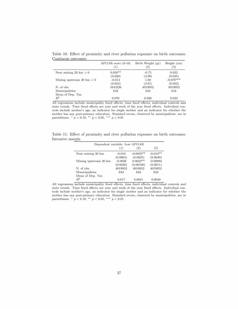
Table 10: Effect of proximity and river pollution exposure on birth outcomes:Continous outcomes

APGAR score (0-10) Birth Weight (gr) Height (cm)(1) (2) (3)

Near mining 20 km > 0 0.050** -0.75 0.022(0.020) (3.99) (0.025)

Mining upstream 20 km > 0 -0.014 1.68 -0.078***(0.024) (3.81) (0.022)

N. of obs. 1643226 4019952 4019952Municipalities 642 642 642Mean of Dep. Var.R2 0.070 0.026 0.033


Table 11: Effect of proximity and river pollution exposure on birth outcomes:Intensive margin

Dependent variable: Low APGAR(1) (2) (3)

Near mining 20 km -0.010 -0.0059** -0.010**(0.0064) (0.0025) (0.0040)

Mining upstream 20 km -0.0026 0.0022** -0.00094(0.0030) (0.00100) (0.0011)

N. of obs. 4019952 4019952 4019952Municipalities 642 642 642Mean of Dep. Var.R2 0.017 0.0041 0.0049


27

Table 12: Effect of proximity and river pollution exposure on birth outcomes

Dependent variable:Low APGAR Low Birth Weight Stunting

Panel A: Exposure up to 20 KMNear mining 20 km > 0 -0.51* 0.019 0.13

(0.27) (0.083) (0.12)Mining upstream 20 km > 0 0.43*** -0.011 0.22**


Panel B: Exposure by distanceNear mining 5 km > 0 -0.71 0.095 -0.11

(0.43) (0.13) (0.20)Near mining 5-10 km > 0 -0.28 -0.035 -0.087

(0.26) (0.11) (0.16)Near mining 10-20 km > 0 -0.48** 0.045 0.26**

(0.24) (0.092) (0.12)Mining upstream 5 km > 0 0.39 -0.019 0.33*

(0.28) (0.14) (0.17)Mining upstream 5-10 km > 0 0.44* -0.18 0.19

(0.26) (0.13) (0.17)Mining upstream 10-20 km > 0 0.45** 0.014 0.22**


All regressions include municipality fixed effects, time fixed effects, individual controls andregional trends. Time fixed effects are year and week fixed effects. Individual controls in-clude mother’s age, an indicator for single mother and an indicator for whether the motherhas any post-primary education. The regional trends allow for a trend for each geographicregion (Pacific, Andean and Caribbean). Standard errors, clustered by municipalities, are inparentheses. ∗ p < 0.10, ∗∗ p < 0.05, ∗∗∗ p < 0.01

28

B Extra Figures

●

●

●

●

●

●

●●

●

●

●

●

●

●

●

●

●

●

●

●

● ●

●

●

2007 2008 2009 2010 2011 2012

0.01

0.02

0.03

0.04

Gold mining activity and heavy metal poisoning

Date

SIV

IGIL

A −

rat

e pe

r 10

0,00

0 in

divi

dual

s

5.0e

+06

1.0e

+07

1.5e

+07

Kg

● SIVIGILA − Heavy metal poisoningGold Production (Kg)

Figure 4:Prevalence of mercury-related health events and gold mining. The solid black line representsthe prevalence of mercury poisoning in Colombia per 100,000 individuals. The dotted redline represents gold production in the country. Source: Authors’ calculations using HealthMinistry data.

B.1 Impacts of different levels of mining

Given that we have the exact shape, size and location of each mine we canestimate the impact of different levels of mining activity, by deciles of the dis-tribution of mining. In other words we estimate the following equation

Yimt =

10∑d=1

βdqdmt +Ximtα+ γm + γt + λr(m) × t+ εimt, (4)

where qdmt indicates whether municipality m at time t is at the decile d ofproportion of mined area. Notice that qdmt = 0,∀d for any municipality m attime t that has no mining titles. Figure 8 shows that the effect is similar forall deciles and we can not reject the null hypothesis that the coefficient βd areall equal to each other, suggesting that the net effect of mining on newborns’health is positive and the same for all levels of mining. In other words, miningbrings benefits, but higher levels of mining do not bring additional benefits.

29

Figure 5: Proportion of births near and downstream from a mine - 5 KM buffer.2

.3.4

.5.6

.7Bi

rths

2000m1 2002m1 2004m1 2006m1 2008m1 2010m1 2012m1Date

Near mining Upstream mining

Births near and downstream from a mine - 0-5 KM

0.2

.4.6

.8M

unic

ipal

ities

2000m1 2002m1 2004m1 2006m1 2008m1 2010m1 2012m1Date


Municipalities near and downstream from a mine - 0-5 KM

This figures shows the number of births and municipalities near/downstream from a mine usinga buffer of 5 KM. The left panel has the proportion of births in our data near/downstream froma mine. The right panel has the proportion of municipalities in our data near/downstreamfrom a mine.

Figure 6: Proportion of births near and downstream from a mine - 10 KM buffer

.05

.1.1

5.2

Birt

hs

2000m1 2002m1 2004m1 2006m1 2008m1 2010m1 2012m1Date


Births near and downstream from a mine - 0-5 KM.0

8.1

.12

.14

.16

Mun

icip

aliti

es

2000m1 2002m1 2004m1 2006m1 2008m1 2010m1 2012m1Date



This figures shows the number of births and municipalities near/downstream from a mineusing a buffer between 5 and 10 KM. The left panel has the proportion of births in our datanear/downstream from a mine. The right panel has the proportion of municipalities in ourdata near/downstream from a mine.

Figure 7: Proportion of births near and downstream from a mine - 20 KM buffer

.05

.1.1

5.2

.25

Birt

hs

2000m1 2002m1 2004m1 2006m1 2008m1 2010m1 2012m1Date


Births near and downstream from a mine - 10-20 KM

.12

.14

.16

.18

.2.2

2M

unic

ipal

ities

2000m1 2002m1 2004m1 2006m1 2008m1 2010m1 2012m1Date



This figures shows the number of births and municipalities near/downstream from a mineusing a buffer between 10 and 20 KM. The left panel has the proportion of births in our datanear/downstream from a mine. The right panel has the proportion of municipalities in ourdata near/downstream from a mine.

30

-3-2

-10

1C

oeffi

cien

t on

low

AP

GA

R

1 2 3 4 5 6 7 8 9 10Decile

Deciles

Figure 8: Mined area and APGAR

Impact of different levels of mining activities on the probability of being born with low AP-GAR. The figure plots the coefficients of dummy variables that indicate whether the miningactivity (proportion of mined area) is in a given decile. The bars indicate 95% confidenceintervals. See equation 4

31

Documents

The E ects of Gold Mining on Newborns’ Healthsantisap/Paper_mining_newborn_health.pdf · The E ects of Gold Mining on Newborns’ Health Mauricio Romero and Santiago Saavedra August