The Effects of Merit-Based Financial Aid on Drinking in

College

Benjamin W. Cowan†§and Dustin R. White‡§

June 23, 2015

Abstract

We study the effect of state-level merit aid programs (such as Georgia’s HOPEscholarship) on alcohol consumption among college students. Such programs havethe potential to affect drinking through a combination of channels–such as raisingstudents’ disposable income and increasing the incentive to maintain a high GPA–thatcould theoretically raise or lower alcohol use. We find that the presence of a meritaid program in one’s state generally leads to an overall increase in (heavy) drinking.This effect is concentrated among men, students with lower parental education, olderstudents, and students with high college GPA’s. Our findings are robust to severalalternative empirical specifications including event-study analyses by year of programadoption. Furthermore, no difference in high-school drinking is observed for studentsattending college in states with merit-aid programs.JEL Codes: I18, I23

Keywords: merit aid; financial aid; alcohol; drinking; college

†Corresponding author. Assistant Professor, School of Economic Sciences, Washington State University.Address: PO Box 646210, Hulbert Hall 101, Pullman WA 99164 USA. Phone: (509) 335-2184. Email:ben.cowan@wsu.edu.

‡Ph.D. candidate, School of Economic Sciences, Washington State University. Address: PO Box 646210,Hulbert Hall 101, Pullman WA 99164 USA. Email: dustin.r.white@wsu.edu.

§We are very grateful to Toben Nelson for providing us with the College Alcohol Study data for thisproject. We also thank Laura Argys, Angela Fertig, and Robert Rosenman for helpful comments andconversations about the paper. All errors are the authors’ alone.

1 Introduction

Heavy drinking among U.S. college students remains widespread even after several decades

of efforts aimed at curbing young people’s alcohol use (Hingson, 2010). Researchers have

made significant progress toward understanding how public policies designed to discourage

(risky) alcohol use shape youth drinking patterns (see, for example, Carpenter et al., 2007),

but other policies that indirectly affect youths’ drinking may not be as well understood.1

Perhaps surprisingly, few studies have examined how student financial aid affects drinking

behavior among college students.2 Though alcohol appears to be a normal good in the

general population (Ruhm and Black, 2002) and among young adults (Nelson, 2008), little

is known about college students in particular. Government and institutional financial aid

programs are not only an important determinant of student disposable income but may

create other incentives that influence alcohol use (by affecting time allocation, for example).

Because these effects are subtle, financial aid programs may affect college drinking in ways

that are currently unknown to policymakers.

This paper examines how one type of financial aid policy, state-level “merit aid” pro-

grams, affects alcohol use among college students. We believe we are the first to examine

1Those policies that explicitly address drinking include the minimum legal drinking age, policies affectingdriving under the influence, and alcohol taxes. In addition, a budding literature on how peers affect substanceuse (including drinking) has made strides toward understanding that dimension of youth risky behavior (see,for example, Kremer and Levy, 2008 and Eisenberg et al., 2014).

2Recent studies that examine the relationship between income and drinking among teenagers includeAdams et al. (2012), who find that higher minimum wages are associated with an increase in alcohol-relatedtraffic fatalities among teens. Markowitz and Tauras (2009) estimate a substantial effect of adolescentallowances from parents on drinking participation–a $1,000 annual increase in allowance is associated with a2.2-7.1 percentage point increase in the probability of drinking. Grossman and Markowitz (2001) is one of theonly studies to estimate an income elasticity (albeit with state-level income per capita rather than individualincome measures) of alcohol use (number of drinks) for college students–they find that this elasticity is 0.63.In addition, Delaney et al. (2008) use cross-sectional Irish data to show that college students’ disposableincome is positively related to alcohol expenditure but not to drinking participation or degree of excessivedrinking.

1

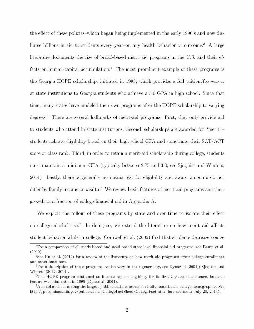
the effect of these policies–which began being implemented in the early 1990’s and now dis-

burse billions in aid to students every year–on any health behavior or outcome.3 A large

literature documents the rise of broad-based merit aid programs in the U.S. and their ef-

fects on human-capital accumulation.4 The most prominent example of these programs is

the Georgia HOPE scholarship, initiated in 1993, which provides a full tuition/fee waiver

at state institutions to Georgia students who achieve a 3.0 GPA in high school. Since that

time, many states have modeled their own programs after the HOPE scholarship to varying

degrees.5 There are several hallmarks of merit-aid programs. First, they only provide aid

to students who attend in-state institutions. Second, scholarships are awarded for “merit”–

students achieve eligibility based on their high-school GPA and sometimes their SAT/ACT

score or class rank. Third, in order to retain a merit-aid scholarship during college, students

must maintain a minimum GPA (typically between 2.75 and 3.0; see Sjoquist and Winters,

2014). Lastly, there is generally no means test for eligibility and award amounts do not

differ by family income or wealth.6 We review basic features of merit-aid programs and their

growth as a fraction of college financial aid in Appendix A.

We exploit the rollout of these programs by state and over time to isolate their effect

on college alcohol use.7 In doing so, we extend the literature on how merit aid affects

student behavior while in college. Cornwell et al. (2005) find that students decrease course

3For a comparison of all merit-based and need-based state-level financial aid programs, see Baum et al.(2012).

4See Hu et al. (2012) for a review of the literature on how merit-aid programs affect college enrollmentand other outcomes.

5For a description of these programs, which vary in their generosity, see Dynarski (2004); Sjoquist andWinters (2012, 2014).

6The HOPE program contained an income cap on eligibility for its first 2 years of existence, but thisfeature was eliminated in 1995 (Dynarski, 2004).

7Alcohol abuse is among the largest public health concerns for individuals in the college demographic. Seehttp://pubs.niaaa.nih.gov/publications/CollegeFactSheet/CollegeFact.htm (last accessed: July 28, 2014).

2

enrollments and increase withdrawals in response to HOPE, perhaps to keep their GPA

above the scholarship renewal threshold. Sjoquist and Winters (2014) estimate that merit-

aid scholarships reduce the number of college students in STEM majors, likely due to their

higher degree of difficulty (Dee and Jackson, 1999). Cornwell and Mustard (2007) find

that the advent of HOPE led to an increase in car sales in wealthier Georgia counties,

presumably because the scholarship is simply a rent payment to families who were planning

to send children to college in the first place. Indeed, income effects associated with merit-

aid programs are expected to be large for many families since the vast majority of those

students who qualify very likely would have gone to college even in the absence of the

program (Cornwell et al., 2006).

Student disposable income might increase as a result of a merit-aid program if parents

and children share the financial gain associated with not having to pay tuition. Other things

equal, this should lead to an increase in drinking if alcohol is a normal good among college

students. However, the preceding paragraph makes it clear that merit-aid programs have the

potential to affect drinking through channels other than a simple income effect: for example,

since these programs increase the incentive to maintain a GPA above the minimum renewal

point in one’s state, merit aid could discourage drinking (particularly for those individuals

who are near or expect to be near the GPA cutoff). Indeed, recent research (for example,

Williams et al., 2003; Carrell et al., 2011; Lindo et al., 2012) suggests that alcohol use has

a negative causal effect on academic performance. If individuals recognize the link between

drinking and grades, they may choose to curb their alcohol use in order to keep their merit

scholarship.

Another pathway by which merit aid might affect college alcohol use is through changes

3

in the allocation of time. Previous research suggests these programs affect choice of major,

which could in turn affect time spent studying. It is conceivable that these programs also af-

fect decisions about how much to work for pay or engage in various extracurricular activities,

any of which could in turn influence drinking behavior. Lastly, the added stress associated

with trying to maintain their scholarship could cause some students to drink more as a way

of self-medicating (see, for example, Economos et al., 2008).

A disadvantage of our study, due to limitations on the variables available in the data, is

that we cannot pinpoint the exact mechanism by which merit aid affects alcohol consumption.

However, we believe this is offset by several advantages. Our data for this project, the College

Alcohol Study (CAS), was designed to capture nationally representative detailed data on the

drinking habits of college students. Furthermore, the 1990’s saw several states adopt large-

scale merit-aid programs at various points. Because CAS data was collected in 1993, 1997,

1999, and 2001, we are able to observe drinking in non-merit and merit states both before

and after the implementation of several of these policies. Thus, we believe our study is ideal

for measuring the overall effect on drinking of merit-aid scholarship programs.

We consistently find that large-scale merit aid programs led to an increase in drinking

among college students living in states that adopt programs. Our preferred specification

indicates that the arrival of a merit-aid program leads to an 18% increase in the number

of days a male student had 5 or more drinks in a row in the past 2 weeks. Effects for

female students overall are generally smaller or even negative (sex differences in our results

is something we discuss in detail in Section 4). We also find that the effects are strongest

for students with lower parental education, older students, and students with high college

grades (recall that a sufficiently high GPA is necessary to maintain a merit scholarship).

4

Our identification strategy rests on the assumption that unobservable trends across merit-

aid states and non-merit states are the same–if this is the case, the differential drinking trends

in merit-aid states are due to the programs themselves. To guard against the possibility that

unseen factors are responsible for the results, we examine the robustness of our results with

respect to the set of control variables used (including state and region-specific trends) as well

as the sample of states used in estimation (for example, only southern states or only states

that eventually adopt a merit-aid program). In addition, we explictly analyze how drinking

trends in merit-aid states compare to other states in an event-study framework. Our main

results are robust to all of these specification changes.

Lastly, we are mindful of the fact that since we only observe individuals’ states of residence

while they are in college, there is a possibility that drinking at institutions in merit-aid states

increases simply because the composition of enrollees changes relative to institutions in non-

merit states (if this were the case, the adoption of a merit-aid program might increase alcohol

use at certain institutions but would not have caused any individual student to change her

drinking habits).8 We can examine this issue indirectly because we have data on college

students’ (retrospective) drinking behavior in high school. We find that students who are

eligible (based on their age) and live in merit-aid states do not report relatively higher levels

of high-school alcohol use (even though they do, of course, report more drinking as college

students). This is evidence that the positive drinking effects we find are not simply due to

institutions in merit-aid states admitting a greater share of heavier-drinking students after

8Our sample consists of students at four-year institutions, which are generally likely to become morecompetitive, if anything, after the adoption of merit aid since some students who would have gone out-of-statefor college now remain in-state (Cornwell et al., 2006 finds this is true in Georgia). Since higher-achievinghigh-school students drink less than their peers on average (e.g. Balsa et al., 2011), this could bias our(positive) estimates toward zero.

5

the program is adopted.

2 Empirical Model

As we argue in Section 1, a merit-aid scholarship program in one’s state of residence has

the potential to change a student’s disposable income, the “full” price of consuming alcohol

(because alcohol use may lower academic performance, which in turn raises the risk of losing

the scholarship), time allocation, and other factors related to drinking. We observe neither

parental nor student income in our data and very little on time allocation. Furthermore, we

do not observe students’ expectations on how alcohol consumption affects their grades. As

a result, we are constrained to examine the “reduced-form” effect of merit-aid programs on

college students’ alcohol use:

ACicst = ζMAist + αs + βt +Xitγ + Zstλ+ εicst, (1)

where ACicst is alcohol consumption by individual i at college c in state s in year t. MAist is

an indicator for the presence of a merit-aid program in state s in year t for those who were

college freshman in the year of implementation or after.9 αs is a state fixed effect, βt is a

year fixed effect, Xit are pre-college individual characteristics, Zst are state characteristics,

and εicst is the regression error.

ζ is identified by comparing the (regression-adjusted) difference in alcohol consumption

between the pre-law and post-law periods in states that adopt programs with the same

difference in non-adopting states (including states that have yet to adopt a program but do

9We do not observe merit scholarship receipt at the individual level in our data.

6

eventually). As described in Section 4, we use a variety of controls and falsification exercises

to account for the possibility that drinking trends in merit-aid states may have been different

than those in non-adopting states even in the absence of a program.

As described in Sjoquist and Winters (2012, 2014), the merit-aid programs adopted by

states over the time period in this study are heterogeneous in terms of generosity. Some

programs, such as the HOPE scholarship in Georgia, offer relatively large amounts of aid

to a majority of high-school graduates. Many other programs are much smaller in scope

(either going to only the very most elite students, providing significantly smaller subsidies,

or both). These latter programs are obviously not expected to have as large of an impact

as the bigger programs. Sjoquist and Winters (2014) classify programs into “strong” and

“weak” categories, and we follow their definition in this paper. We include Table 1 from

their paper in our Figure 1, which provides details on the 9 strong programs and lists the 18

weak programs adopted since the early 1990’s.

Like Sjoquist and Winters (2014), Dynarski (2008), and Hickman (2009), we define our

treatment according to whether an individual is eligible (a college freshman in the first year

the program goes into effect or after) to receive merit aid in a state with a strong merit-

aid program. We include individuals from states with weak programs in the control group

but also perform specifications in which they are excluded from the analysis.10 Of the 9

“strong” merit-aid states, 6 see a change in merit-aid status in the CAS data (Georgia,

Florida, Kentucky, Louisiana, New Mexico, and South Carolina) because Tennessee and

10An alternative is to include separate dummies for both strong and weak merit-aid eligibility. We also triedthis specification and found it made little difference in the treatment effect of strong merit aid. Anotherpossibility is to examine the effect of merit aid on the intensive margin by using award amounts (perundergraduate, for example) on the right-hand side. However, awards per undergraduate are fairly similaracross strong-merit states and often do not vary much within a state over time (though there are exceptions).Thus, we focus on the presence of a large-scale merit-aid program as our variable of interest.

7

West Virginia change status after the last year of CAS (2001) and there are no observations

from Nevada in the data.11

An important question related to the size of the income effect generated by these programs

is whether merit-aid scholarships crowd out other forms of aid or lead to increases in higher

education costs that are not covered by the scholarship (e.g. room and board). Indeed,

Long (2004) finds some evidence of an acceleration in higher education costs due to merit-

aid programs. However, Dynarski (2004) argues that total educational spending in Georgia

rose substantially following the passage of HOPE, while Doyle (2010) finds that merit-aid

programs have not led to a reduction in need-based aid among adopting states. This may

partly be due to the fact that large merit-aid programs have often been funded by newly

established lotteries (Dynarski, 2004). Singell Jr et al. (2006) actually find that total Pell

Grant awards increased in Georgia following the passage of HOPE, suggesting that merit

aid has been useful in leveraging more need-based support for poorer students (rather than

crowding out such aid). Nevertheless, to the extent that institutional or other government

need-based aid is crowded out by merit aid, we would expect the largest income effects of

merit-aid programs to accrue to wealthier students’ families (who are also most likely to be

inframarginal with respect to the decision to attend a four-year institution).

Another relevant question concerning how much student income rises under a strong

merit-aid program is how parents and children split the windfall that accompanies a program.

Certainly parents may reduce their total level of financial support when their child is given

a full tuition/fee waiver, but what likely matters most with respect to alcohol consumption

is what happens to the child’s disposable income. To extract a larger share of the merit-aid

11We take up issues related to statistical inference when the number of treatments is small in Section 4.1.

8

rents for themselves, students with generous parents in merit-aid states can threaten to go

to an out-of-state institution (in which case the parental financial burden rises significantly).

This should cause parents to give their children “a better deal” to stay in their home state

for college.

3 Data

The dataset used throughout our analysis is the College Alcohol Study (CAS). CAS is

a nationally representative cross-sectional survey of four-year, full-time college students in

1993, 1997, 1999, and 2001. In each year, the sample is comprised of roughly 14,000 students

from 120 institutions in 40 states.12 CAS has a long history in economic and public health

research (see Wechsler and Nelson, 2008). CAS is ideal for this study in that it contains

detailed information on college students’ drinking behavior and it coincides with a period of

rapid expansion of merit-aid programs in the United States. We provide additional details

on the survey design in Appendix B.

Our principal measure of alcohol consumption (our dependent variable) is a measure of

heavy or “binge” drinking: the number of days in the past 2 weeks in which a student had 5 or

more alcoholic drinks in one sitting.13 This kind of drinking has been found to be especially

associated with harmful behaviors and outcomes (see, for example, Wechsler et al., 2002).

In robustness checks, we use other measures of consumption: a binary variable indicating

whether the individual engaged in binge drinking in the past 2 weeks, a binary variable

12See http://archive.sph.harvard.edu/cas/About/index.html (last accessed: July 28, 2014).13Possible answers to this question in CAS were 0, 1, 2, 3-5, 6-9, and 10 or above. We re-code these as 0,

1, 2, 4, 7.5, and 10, respectively.

9

indicating whether the student drank alcohol in the past month, and the total number of

drinks a student had in the past month (days drank alcohol in the past month multipled by

average number of drinks per day in which drinking occurred).

CAS allows us to use a rich set of control variables in our analysis. In most of our specifi-

cations, we include controls for individual characteristics that are plausibly “pre-determined”

at college entry: dummies for age, race/ethnicity, sex, year in school, father’s college atten-

dance, mother’s college attendance, and religious affiliation. To deal with the possibility that

strong merit-aid states differ from other states in unobserved ways, we include state and year

fixed effects in all specifications and additional state and region trends in some specifications

(this is described in the next section). We also include time-varying state characteristics

that may affect alcohol use: median income, unemployment rate, and tax rate on liquor.

In limited robustness checks, we control for individual and institutional characteristics

that are likely determined after merit-aid receipt (“post college”): dummies for marital sta-

tus, living off-campus, being a member of a fraternity/sorority, current college GPA (dum-

mies for A, A-, B+, B, B-, C+, C, C-, and D), whether the institution is public, whether

it is rural, whether it is a commuter school, whether it has a religious affiliation, school size

(4 categories), and school competitiveness (8 categories). These variables are potentially

endogenous to the treatment (merit aid adoption) and are thus only used to examine the

robustness of our main results. Descriptive statistics on all variables used in our regression

analysis are shown for all college students as well as males and females separately in Table 1.

Since CAS is not a well-known data source in the economics literature, we compare our

drinking measures to those reported for college students in Monitoring the Future (MTF)

and several student characteristics to those reported for college students in the National

10

Longitudinal Survey of Youth, 1997 cohort (NLSY97). In Table 2, we display the percentage

of college students who drank in the past month and the percentage reporting at least one

episode of binge drinking (5+ drinks) in the past 2 weeks in both CAS and MTF. For each

year, the MTF figures come from Tables 9-3 and 9-4 in Johnston et al. (2004).14 As seen

in the table, both drinking and binge drinking rates are fairly stable over the sample period

(1993-2001) and are very similar across the two datasets.

Table 3 shows how drinking measures and student demographics compare between the

1999 and 2001 waves of CAS and the same years of the NLSY97. We chose these two years

because a significant number of NLSY97 respondents were college-aged in 1999 and 2001

(and they overlap with the last two waves of CAS). Our NLSY97 sample is restricted to

those who were attending four-year colleges in those years. As seen in Table 3, we calculated

means of drinking and demographic variables that were common across the surveys. The

NLSY97 figures are weighted to account for the fact that it oversamples certain subgroups

(e.g. minorities).

Once again, drinking measures (consuming alcohol in the previous month, total number

of drinks in the previous month) are similar across the surveys overall.15 When the results

are broken out by gender, it appears that CAS women drink somewhat less than NLSY97

women. Both studies indicate a large gender difference in total number of drinks, a result

that is consistent with other studies (Wilsnack et al., 2009). Demographics are also similar

across the data sources, with females having slightly higher representation in CAS while

blacks have lower representation. Since there are more Hispanics in CAS, perhaps part

14The number of binge days is not reported in Johnston et al. (2004), so we cannot compare those figureswith ours.

15The NLSY97 asks individuals about binge drinking over the previous month rather than 2 weeks (as inCAS), so those figures are not directly comparable.

11

of these differences are due to variations in how the two studies elicit race and ethnicity.

CAS students are a little more likely to have had parents who attended college (particularly

fathers). Region representation is fairly consistent across CAS and the NLSY97. Overall, we

believe CAS is similar to these other (more familiar) data sources, both in terms of alcohol

use and other variables, such that the results that follow are not particular to the dataset

chosen for this analysis.

4 Results

4.1 Baseline results

The baseline results of the paper–with number of heavy drinking days in the past 2 weeks

as the dependent variable–are shown in Table 4. All models are estimated with CAS data

via OLS. Each column shows the effect of merit aid on drinking (for all students, just males,

and just females) from a model with a different set of controls and/or sample, as indicated

in the table.16 All models include observations from weak-merit states in the control group.

Appendix Table 1 displays merit-aid effects from regressions in which these individuals are

excluded from the regressions, and the results are very similar to those contained in Table 4.

Standard errors based on the usual asymptotic approximation (but clustered at the state

level and robust to heteroskedasticity) are reported in parentheses. Asterisks assigned to

coefficients denote statistical significance at various levels based on these standard errors.

However, Conley and Taber (2011) note that inference can be misleading when the number

16Chow Tests of the null hypothesis that male coefficients are the same as female coefficients are typicallyrejected at better than the 1% level in our models. Thus, we always estimate the entire regression modelseparately for males and females when examining the results by gender.

12

of policy changes in the data is small (such that the usual asymptotic approximation is not

appropriate). This critique may be applicable to our study because of the small number of

states (6) that change their merit-aid policy over our sample frame. As a result, in addition

to calculating standard errors based on the usual asymptotic assumptions, we also follow

Conley and Taber (2011) in generating 90% confidence intervals that are based on keeping

the number of treatment groups fixed as an assumption.17 These are reported in brackets

below the coefficients and traditional standard errors.

The first column of Table 4 shows results from a specification with state and year fixed

effects but no additional covariates (other than the merit-aid indicator). There is a statisti-

cally significant (at the 5% level) positive effect of strong merit aid on heavy drinking overall,

and this effect is slightly larger for men (though the point estimates are not significant at

conventional levels for men or women individually). Column 2 adds a set of pre-determined

(pre-college) characteristics as discussed in the previous section. Pre-college variables are

added to the model to account for the possibility that selection into colleges changed fol-

lowing the passage of merit-aid programs in a way that affected alcohol use (this issue is

discussed further when we examine how these characteristics were affected by merit-aid pro-

grams in Section 4.3). In this specification, an economically meaningful gender difference in

the treatment appears (with only males experiencing a statistically significant effect at the

10% level).

With state and year fixed effects in the model, we have controlled for both time-invariant

17We thank John Winters for providing us with his code for performing the Conley-Taber procedure.Under the standard difference-in-differences assumption (random assignment of treatment conditional ongroup and time effects), the random error terms for treatment and control groups have the same distribution.As explained in Conley and Taber (2011) and Sjoquist and Winters (2014), the procedure uses the controlgroups to estimate the CDF of the treatment effect under a specific null hypothesis. Confidence intervalsare based on the appropriate quantiles of this distribution.

13

state-level differences in binge drinking across merit and non-merit states as well as secular

changes in drinking over time. However, the possibility remains that trends in young people’s

drinking behavior would have been different in strong merit-aid states than in control states

even in the absence of the programs. For example, because strong merit-aid states are

concentrated in the south, it may be the case that merit-aid programs are simply masking

a broader differential in trends between southern states and the rest of the U.S. To guard

against this possibility, we add state-specific linear time trends to the model (Column 3 of

Table 4). This results in a substantial separation of the merit-aid effect for men and women,

with men experiencing a larger positive effect and women actually experiencing a negative

effect (though the Conley-Taber 90% confidence interval overlaps zero in the female case).

The gender difference in coefficients is statistically significant at the 5% level (based on

standard asymptotic inference) in Column 3.

Columns 4-7 of Table 4 display results from additional models that further scrutinize the

notion that merit-aid states are different from control states in unobserved ways. Region-

by-year dummies are added to the right-hand side in Column 4, and the results change very

little relative to Column 3. The same is true of Column 5, in which only southern states

are included in the regression sample (the empirical model is the same as in Column 3).

Column 6 reports results from the same model as Column 3 but only with observations from

the 6 strong-merit states included in the analysis (Conley-Taber intervals are not reported

here because all states in the sample are treatment states). It is still possible to identify

the merit-aid effect in this case because treatment states adopt strong merit-aid programs

in different years. Once again, the result are highly consistent with Column 3. Lastly, in

Column 7, the full sample of states is again used but post-college enrollment individual

14

and school characteristics, which are potentially endogenous to merit-aid receipt, are added

to the Column 4 model. The rationale for including this “saturated” model is again the

possibility that the composition of college students in merit states is changing (relative to

non-merit states) over time in a way that might be partially captured by these additional

characteristics. We find yet again that the results first found in Column 3 are highly robust

to the inclusion of these variables.

The results in Columns 3-7 of Table 4 mitigate the concern that treatment states are

fundamentally different from other states and would have experienced a differential trend in

college alcohol use even in the absence of merit aid. Once state-specific trends are included

in the model, the result that males experience a large, positive increase in binge drinking

following merit-aid adoption (and that the effect for females is negative, if anything) is

highly robust. We do not know precisely why the magnitude of the coefficients change

significantly when state-specific trends are controlled for (going from Column 2 to 3), but

we note that their inclusion does reduce the variation in the merit-aid variable with which to

estimate the treatment effect. Nevertheless, the results in Column 2 (without these trends)

are qualitatively similar to those in Column 3 even though the magnitudes differ.

As a whole, the results in Table 4 suggest that males increase their heavy drinking in

response to a strong merit-aid program but females do not. Conley-Taber 90% confidence

intervals do not overlap zero in 6 out of the 7 specifications for males but contain zero in all

specifications for females. Because once state-specific time trends are added to our regression

model the results change very little, we adopt the model described in Column 3 (using the

full sample and with controls for state and year fixed effects, pre-determined individual and

state characteristics, and state-specific linear time trends) as our preferred specification for

15

the remainder of the paper. This specification implies that a merit-aid program increases

male-binge drinking days by about 18% at the mean.

4.2 Other drinking measures

In Table 5, we examine how strong merit aid affects alcohol consumption using alternative

drinking measures: whether the individual consumed alcohol in the past month (Column 1),

the number of drinks in the past month (Column 2), and whether the individual engaged in

binge drinking in the past 2 weeks (Column 3). The last column (4) of Table 5 is simply

Column 3 of Table 4 (with number of binge occasions in the past 2 weeks as the dependent

variable), reproduced for convenience. All models are estimated using our preferred speci-

fication as described in the previous section. As shown in the table, there is essentially no

effect of the treatment on either drinking or binge drinking at the extensive margin for either

gender (Columns 1 and 3). As in the case of binge drinking, however, there is positive and

significant (at the 5% level) effect of merit aid on the intensive margin of drinking (total

number of drinks in the past month) for males. This shows that men in merit-aid states do

not offset more binge drinking with less casual drinking, since the total number of drinks

increases as well. Since we find total number of drinks to be responsive to merit-aid adop-

tion in our preferred specification, we include results from our full set of specifications (as in

Table 4 for binge-drinking occasions) for this dependent variable in Appendix Table 2. The

pattern of results is very similar to the pattern for heavy-drinking days, with total drinks

increasing by about 16% at the mean following treatment for males.

16

4.3 The composition of students

In this section, we address the possibility that merit-aid programs changed the composition

of the student body in four-year institutions (relative to non-merit states). Indeed, Corn-

well et al. (2006) find that SAT scores among incoming freshmen in Georgia public schools

improved relative to the national average following the passage of HOPE, and Henry and

Rubenstein (2002) find evidence of scholastic improvement in the student body in strong-

merit states. If changes in student composition were correlated with drinking behavior,

our results may be due to a changing student body rather than changes in drinking at the

individual level.

Using our preferred empirical specification, we examine how merit-aid programs affects

individual pre-college characteristics in Table 6.18 These programs seem to have no effect

on gender, age, or mother’s college status. However, the probility of a student indicating

her race as “white” rises and the probability of a student’s father having attended college

falls with merit-aid adoption. These effects are small: the increase in the likelihood of

being white is 5% and the decrease in the likelihood of father’s college attendance is 4% at

their respective means. Nevertheless, they indicate some compositional changes that may

influence our results. Importantly, however, our preferred specification controls for these

pre-college factors and still finds a substantial effect on drinking due to merit aid (for men).

The fact that adding a host of additional right-hand side variables that reflect both pre- and

post-college decisions (Column 7 of Table 4) does not affect our results is further evidence

18In addition to individual characteristics, it would be worthwhile to examine whether merit-aid implemen-tation affects a student’s propensity to attend college in particular geographic location (i.e. in a merit-aidstate) or at a particular type of institution (e.g. public instead of private). Unfortunately, CAS’s design,which surveys the same schools over time and samples the same number of individuals at most schools,prevents this type of analysis. See Appendix B for more details.

17

that differences in composition are not responsible for our estimates.

We can also indirectly examine whether merit-aid states were more likely to attract

students with a higher propensity to engage in (binge) drinking by looking at the high-school

drinking habits of individuals who attend college in merit-aid states versus those who do not

(the last column of Table 6). In CAS, respondents are asked how many times, on average,

they drank alcohol per month while still in high school (this is the only question on high-

school drinking). This data is retrospective, so it is subject to some recall bias. Nevertheless,

it provides us with an opportunity to see whether high-school drinking trends follow the same

pattern as college ones–if that were the case, it would suggest that our estimates may simply

be due to changes in the make-up of the sampled student population in merit-aid versus

non-merit states.19

As seen in the last column of Table 6, the effect of merit aid on high-school drinking

days is close to zero for all youth and males and females separately. In fact, this result is

not specific to our preferred specification but is true of all specifications shown in Table 4

(these results are available upon request). These findings lend credence to the notion that

19This analysis is subject to some caveats. First, because drinking for high-school aged students is illegal,and because the vast majority of them are living with parents or other caretakers, it is possible that thereare many “would-be” drinkers in the data that are more likely to attend college in merit-aid states afterprograms are adopted, which this analysis would fail to pick up (since we can only measure actual ratherthan latent drinking). However, over 60% of the students in our sample report at least some positive amountof monthly drinking in high school, so we believe this problem is not serious.

Second, it is theoretically possible that merit aid programs affect high-school drinking if teenagers areaware of their existence and are planning to use them. A merit-aid program raises expected lifetime incomefor those who expect to receive aid (possibly leading to an increase in alcohol consumption) and increasesthe incentive to maintain good grades in high school for those who expect to be near the GPA cutoff (whichmay encourage such students to curb their drinking). It seems unlikely that high-school students are ableto “borrow” against future college aid in a substantial way, but it may be the case that students drink lessto better their chances at a scholarship. Cowan (2011) finds that increased college attendance expectations(through more affordable two-year college tuition) cause teenagers to engage in less risky behavior (includingheavy drinking). In the case of merit aid, the great majority of students who receive a scholarship wouldhave gone to college even without it (Cornwell et al., 2006), which implies this mechanism is likely to playonly a minor role.

18

our earlier results reflect true causal effects of merit-aid programs on college drinking; since

high-school drinking does not follow the same pattern, it is more doubtful that our results

can be explained by changes in college-student composition.

4.4 Event-study analysis

Though our preferred specification discussed in the previous sections includes controls for

state-specific trends, we have not yet explicitly analyzed whether pre- and post-program

trends were different in treatment and control states. To this end, we perform an event-

study analysis and report the results in Table 7. Since the strong-merit states in our sample

adopted programs in different years, we produce a separate analysis for each year in which

at least one state adopted a strong merit-aid program (Georgia in 1993, Florida and New

Mexico in 1997, Louisiana and South Carolina in 1998, and Kentucky in 1999). For each

of those four treatment groups, we compare the state(s) adopting treatment to all control

states (i.e. we exclude states adopting strong merit aid in other years).

Because our treatment is based on cohort (i.e. year of freshman enrollment), we examine

trends in drinking by cohort relative to each policy change.20 Cohort groupings are made

based on when treatment occurred since, for example, there are only a few cohorts in the

data that preceded treatment in Georgia (but several cohorts that followed treatment), and

Kentucky has the opposite situation. For Georgia, we look at four groups: cohorts 1-3 years

prior to the policy change, 1-3 years after, 4-6 years after, and 7 or more years after. For

both Florida/New Mexico and Louisiana/South Carolia, our four groups are: cohorts 4 or

20Because we only observe an individual’s year in college at the time she is sampled, we calculate yearof freshman enrollment (and thus cohort) as the “current year - 1” for sophomores, “current year - 2” forjuniors, “current year - 3” for seniors, “current year - 4” for 5th year seniors, and “current year - 5” for thosein their 6th year or above.

19

more years prior to the policy change, 1-3 years prior, 1-3 years after, and 4 or more years

after. Finally, when looking at Kentucky, we have four groups that are the “mirror image”

of the ones for Georgia: cohorts 7 or more years prior to the policy change, 4-6 years prior,

1-3 years prior, and 1-3 years after.

Table 7 shows results of regressions that contain state fixed effects, dummies for each

of four cohort groupings (which change depending on the year of treatment, as described

above), and the interaction between the cohort grouping dummies and treatment (which is

“1” for the strong merit-aid state(s) in question and “0” otherwise). Each column in the

table shows results for a different treatment group (depending on year of treatment). The

omitted category in every case is “cohorts 1-3 years prior to the policy change.” Because the

treatment samples are so much smaller in this analysis, we do not perform the regressions

separately by gender.

We first look at pre-treatment trends. There is some evidence that heavy drinking is

increasing in control states early on (recall that the coefficients are relative to the effect for

the “1-3 cohorts prior to the policy change” group) but no evidence that those trends are

different in treatment states (see the interactions between cohort groups that fall prior to

the policy change and “strong merit program”). After treatment, there is no clear heavy

drinking pattern in control states; however, there is a sharp, statistically significant (at

the 5% level) increase in drinking in treatment states (relative to control states) for the “1-3

cohorts following the policy change” group in 3 of 4 cases (with Louisiana and South Carolina

in 1998 being the exception). Interactions between “strong merit program” and subsequent

cohort groups are also generally positive, though smaller and less precisely estimated than

for the first three cohorts following policy changes.

20

Although the case of Louisiana/South Carolina is an exception in this specification, the

broad pattern in the trends presented in Table 7 is supportive of the notion that it was

indeed merit-aid programs (rather than some unobservable factor) that led to an increase in

heavy drinking in strong merit-aid states overall. In the next section, we consider how the

effects of merit-aid programs differ across individual characteristics.

4.5 Result heterogeneity

In Section 4.1, we establish that in most of our specifications (including our preferred one)

males appear to experience a larger (positive) drinking response to the introduction of merit

aid than do females. We are also interested in whether our results vary along other dimen-

sions. We initially examine whether there is heterogeneity in the results by pre-determined

characteristics, including race, age, and parental education (Table 8) and then by post-

college characteristics, including college GPA, fraternity/sorority status, and public/private

institution type (Table 9). In each case, our preferred empirical model is used to generate

results for all students as well as men and women separately. Standard errors clustered at

the state level are reported in parentheses.21

4.5.1 Results by pre-college factors

Table 8 shows that the positive effect of merit aid on heavy-drinking days for males is stronger

among whites, students who are 21 or older (the legal drinking age), and students whose

mothers did not attend college. The last two results are especially pronounced. A natural

explanation for the age difference is that student drinking is more susceptible to additional

21Because inference based on asymptotic methods and the Conley-Taber method do not differ substantiallyin our baseline specification, we choose to focus on standard asymptotic inference in this section of the paper.

21

disposable income when drinking is legal. However, reported binge-drinking days are similar

for underage and legally aged males, so this is likely not the full explanation. Another part of

the story may be that younger students, who are typically underclassmen, have more to lose

by failing to renew their scholarship (since they have more college years in front of them),

which would make the grade performance incentive more important for them.

Strikingly, the positive effect of strong merit aid on heavy drinking is highly concentrated

among males whose mothers did not attend college (the corresponding difference in effects

by father’s college attendance is much weaker). Such students are more likely to be first-

generation college students (clearly) and come from lower-income families (Terenzini et al.,

1996). The results presented in Table 6 indicate that the probability of having a college-

educated mother did not change with the adoption of merit-aid programs. Rather, students

with less-educated mothers appear to be most susceptible to the incentives for more heavy

drinking that merit-aid programs create.

4.5.2 Results by post-college factors

Because post-college factors including GPA, fraternity/sorority status, and institution type

may themselves be influenced by merit-aid receipt, the results in this section must be treated

with some caution. Nevertheless, we choose to examine how results differ according to these

variables to further examine our identification strategy (in the case of GPA) and to gain

further insight into the mechanism(s) by which aid affects college drinking.

We begin by examining how the effects of strong merit-aid eligibility vary by college GPA.

Because merit aid is renewed only for those college students who maintain a minimum GPA

22

(see Figure 1), we expect these effects to vary over the GPA distribution.22 To examine

whether this is the case, we divide all students into 3 GPA classifications: 3.4 (B+) or

above, 2.7-3.0 (B- to B), and 2.4 (C+) or less. The first group is most likely to be on

scholarship (a 3.4 GPA qualifies for renewal in all strong merit states) and might also be

relatively unconcerned with scholarship loss, since (marginal) reductions in grades due to

increased alcohol consumption would likely not move them below the GPA threshold for

renewal (generally between 2.5 and 3.0 depending on the state and year in school).23

The next group is the “marginal” group (2.7-3.0): many of these individuals would be

eligible for merit aid in strong states, but poor performance could cause one’s GPA to dip

below the renewal point, so the grade performance effect may be more important than it

is for the first group. Lastly, many of those in the third category (2.4 or less) will not

be on merit scholarship, either because they never received it initally or have since lost it

(renewal is determined annually in most states). Some states with strong merit programs

allow individuals who have lost the scholarship to regain it by raising their GPA above the

renewal threshold; for this reason, individuals in this category who live in strong merit states

might have an incentive to reduce their alcohol consumption to improve their grades.

The results from regressions run separately by GPA category are contained in Table 9.

Once again, large differences in the coefficients are observed for men and women. Men in

the highest GPA category experience a large, significant (at the 1% level) increase in heavy

22Unfortunately, CAS does not contain data on high-school grades, which determine initial receipt of meritaid.

23Another way of thinking about this analysis is as a difference-in-differences in which the control group isstudents who would have been eligible for merit aid had they lived in a state with a strong merit-aid program.Unfortunately, a regression discontinuity design, in which students just above and just below the renewalGPA cutoff are compared, is not feasible here because we lack sufficient precision in our GPA measure andhave no data on individual receipt of the scholarship.

23

drinking days. This is in line with there being a relatively large boost to income for this group

without much concern for falling below the scholarship renewal point. The point estimate for

men in the middle GPA category is actually a bit higher than the one for the high category,

though it is less precisely estimated. Men in the bottom GPA category experience a negative

but statistically insignificant effect of merit aid on heavy drinking. Thus, the pattern in the

results for men is largely consistent with what we would expect given how incidence of the

scholarship should be concentrated among individuals with higher college GPA’s.

The story for women is clearly different, as no GPA group of female students show

positive, statistically significant merit-aid effects. Furthermore, point estimates are actually

somewhat larger for those with lower grades. Though an in-depth analysis of the gender

difference in drinking response to merit aid is beyond the scope of this paper, we note some

facts that are likely to be relevant. Female and male drinking habits differ markedly, with

males typically drinking more often and more heavily in many countries (Wilsnack et al.,

2009).24 Researchers have found gender differences in drinking responses to interventions

other than changes in financial aid–for example, Kremer and Levy (2008) find that males

are more susceptible than females to being assigned a heavily drinking roommate in college.

Our results may be the result of a difference in income elasticities for alcohol between men

and women or differences in the relative size of the income, grade performance, and/or

other incentives of merit-aid programs across sex. Other researchers have found large gender

differences in how underage youths obtain alcohol, with males being much more likely to get

it from a commercial outlet and females being more likely to get it from someone age 21

24In our data, female alcohol consumption is about half of male alcohol consumption by both intensivemeasures (number of days of 5 or more drinks and total number of drinks in the past month).

24

or older (Wagenaar et al., 1996). This could translate into differences in income elasticity,

though we do not know of estimates that support or fail to support that possibility. This is

a question for future research.

The remainder of Table 9 shows how our results vary by fraternity/sorority membership

and institution type (public or private). We find that the positive heavy drinking effect

of merit aid are concentrated among non-greek males (i.e. those not in a fraternity). In

our sample, both men and women who hold greek membership drink about twice as much,

on average, as do non-greek students. Furthermore, Walker et al. (2014) finds that greek

students come from higher-income families than do non-greek students. Our results are

consistent with the notion (not tested in this paper) that there is more scope for merit aid

to affect the disposable income and drinking behavior of non-greek youths.

Lastly, students at public institutions experience drinking increases after merit aid while

students at private institutions do not. It is notable that though most strong-merit states

provide merit-aid subsidies for private (in-state) college attendance, they are typically smaller

than those for public attendance, often in absolute terms and as a fraction of tuition (Dy-

narski, 2004).

Because we lack the data in CAS, we cannot directly examine how our baseline results

compare for students in different family income brackets. However, the results in this section–

including the findings that heavy drinking responses are stronger for students who do not

belong to fraternities/sororities, have mothers who did not attend college, and are enrolled

in public institutions–may be indicative of merit aid having a larger effect on the behavior

of student with more modest family incomes. This could be happening for several reasons,

among them the possibility that merit aid raises the disposable income of these students,

25

while students from richer families may already have (relatively) high disposable incomes to

begin with and thus do not see much change with the passage of merit-aid laws.

5 Conclusion

We study the effects of state-level merit-based scholarship programs on the drinking behavior

of college students. We find that, on average, a strong merit-aid program leads to an increase

in male alcohol consumption according to two measures: the number of days in the past 2

weeks that an individual had 5 or more drinks on one occasion and the total number of

alcoholic drinks over the past month. These effects are not uniform across the student

population; rather, they are especially concentrated among men, students with high GPA’s,

students with non-college mothers, and older students.

Based on the information on strong merit-aid programs provided in Sjoquist and Winters

(2014) (reproduced in Figure 1 of this paper), the (population-weighted) average subsidy in

strong merit states is roughly $1,000 per student (or roughly $3,000 per recipient). We find

that a strong merit-aid program raises male heavy drinking by about 18%. However, we

cannot derive an income elasticity (or semi-elasticity) of alcohol use among college students

because merit-aid programs have the potential to affect drinking through several alternative

pathways (e.g. by changing time-use incentives) and our data is limited. Nevertheless, we

view this paper as a step toward understanding how financial aid programs affect risky

behavior among college students, a topic that is largely unexplored in the literature. Future

work on merit-aid programs could disentangle how income and grade performance incentives

as well as other factors account for higher drinking in merit-aid states. Furthermore, because

26

other financial aid programs differ in structure and incentives (for example, need-based aid),

more work is needed to comprehend how financial aid can be designed to minimize deleterious

effects on student risky behavior as it strives to meet its primary objectives.

A Appendix: Background information on merit-aid

programs

U.S. federal grant aid for college is heavily based on financial need (for example, Dynarski,

2004 states that 90% of dependent students who receive federal grants grew up in families

with annual incomes of less than $40,000). State-based financial aid was also traditionally

based on need–roughly 90% was at least partly need-based in 1992-93–but with the adop-

tion of large-scale merit-based financial aid programs in several states since that time, that

percentage had fallen to about 70% as of 2010 (Baum et al., 2012).

Merit-aid programs are designed to provide funding to the highest-achieving students in

order to keep the “best and brightest” in their home state for college (Zhang and Ness, 2010).

These programs typically do not consider financial need as a criterion for award receipt.

One of the earliest and best-known examples is the Georgia Helping Outstanding Pupils

Educationally (HOPE) scholarship, which provides a full tuition waiver at in-state public

institutions for students who receive a qualifying 3.0 GPA in high school (smaller awards are

also available at in-state private institutions). The Georgia Student Finance Commission

states that $5.8 Billion have been distributed since 1993 through the HOPE scholarship

program to approximately 1.4 million students.25 Merit-aid programs in other states differ

25See http://www.gsfc.org/gsfcnew/HopeProgramm.cfm (last accessed: February 20, 2015).

27

in terms of qualification criteria and the size of awards, but they are overwhelming tied to

in-state college attendance (though at least one program, the Louisiana TOPS program, is a

partial exception to this). As of 2012, 24 states awarded scholarships through a merit-based

aid program, though programs varied greatly in size (Sjoquist and Winters, 2012).

The bulk of the academic literature on merit-aid programs focuses on their effects on

1) in-state college attendance and residence after schooling is completed, 2) overall college

enrollment, and 3) overall college completion. This literature is reviewed in Hu et al. (2012).

Our reading of the literature is that merit-aid programs do seem to increase in-state retention

of students (even after college, at least modestly–see, for example, Hickman, 2009); however,

the effect of aid on overall enrollment and (especially) completion is mixed. For example,

Dynarski (2008) find positive completion effects (of HOPE), but Sjoquist and Winters (2012)

find no such effects when examining all large-scale merit-aid programs. Typical estimates are

that large merit-aid programs raise college enrollment/completion by less than 10 percentage

points, if at all; thus, the vast majority of affected students are infra-marginal with respect

to college attendance (Cornwell et al., 2006).

B Appendix: Background information on the College

Alcohol Study

A full description of the survey design for the College Alcohol Study is contained in Wechsler

et al. (1994). CAS began with 179 accredited four-year college institutions chosen with

probability proportionate to enrollment size. 140 of these institutions participated. Because

28

smaller schools (enrollment less than 1,000) were less likely to participate, an over-sample

of smaller institutions was added to the study. A sample of 215 full-time, undergraduate

students was drawn from most CAS schools but 108 students were drawn from the very

smallest schools. Roughly 70 percent of sampled students completed the initial (1993) survey.

In subsequent surveys (1997, 1999, and 2001), students were again sampled (using sim-

ilar procedures) from the same institutions that participated in the 1993 survey. The vast

majority of institutions continued to participate, and though a small number were dropped

due to insufficient response rates, binge drinking was found to be very similar with and

without those that were dropped (Wechsler et al., 1998, 2000, 2002). These subsequent CAS

surveys again represented a national cross section of four-year colleges in their respective

years (Wechsler et al., 1998, 2000, 2002).

References

Adams, S., M. L. Blackburn, and C. D. Cotti (2012): “Minimum Wages and Alcohol-Related Traffic Fatalities among Teens,” Review of Economics and Statistics, 94, 828–840.

Balsa, A. I., L. M. Giuliano, and M. T. French (2011): “The Effects of Alcohol Useon Academic Achievement in High School,” Economics of Education Review, 30, 1–15.

Baum, S., D. W. Breneman, M. M. Chingos, R. G. Ehrenberg, P. Fowler,J. Hayek, D. E. Heller, et al. (2012): “Beyond Need and Merit: StrengtheningState Grant Programs,” Washington: Brookings Institution, Brown Center on EducationPolicy.

Carpenter, C. S., D. D. Kloska, P. O’Malley, and L. Johnston (2007): “AlcoholControl Policies and Youth Alcohol Consumption: Evidence from 28 Years of Monitoringthe Future,” The BE Journal of Economic Analysis & Policy, 7.

Carrell, S. E., M. Hoekstra, and J. E. West (2011): “Does Drinking Impair CollegePerformance? Evidence from a Regression Discontinuity Approach,” Journal of PublicEconomics, 95, 54–62.

Conley, T. G. and C. R. Taber (2011): “Inference with Difference in Differences with aSmall Number of Policy Changes,” The Review of Economics and Statistics, 93, 113–125.

29

Cornwell, C. and D. B. Mustard (2007): “Merit-Based College Scholarships and CarSales,” Education Finance and Policy, 2, 133–151.

Cornwell, C., D. B. Mustard, and D. J. Sridhar (2006): “The Enrollment Effectsof Merit-Based Financial Aid: Evidence from Georgias HOPE Program,” Journal of LaborEconomics, 24, 761–786.

Cornwell, C. M., K. H. Lee, and D. B. Mustard (2005): “Student Responses toMerit Scholarship Retention Rules,” Journal of Human Resources, 40, 895–917.

Cowan, B. W. (2011): “Forward-thinking Teens: The Effects of College Costs on Adoles-cent Risky Behavior,” Economics of Education Review, 30, 813–825.

Dee, T. S. and L. A. Jackson (1999): “Who Loses HOPE? Attrition from Georgia’sCollege Scholarship Program,” Southern Economic Journal, 379–390.

Delaney, L., C. Harmon, and P. Wall (2008): “Behavioral Economics and DrinkingBehavior: Preliminary Results from an Irish College Study,” Economic Inquiry, 46, 29–36.

Doyle, W. R. (2010): “Does Merit-based Aid “Crowd Out” Need-based Aid?” Researchin Higher Education, 51, 397–415.

Dynarski, S. (2004): “The New Merit Aid,” in College Choices: The Economics of Whereto Go, When to Go, and How to Pay for It, University of Chicago Press, 63–100.

——— (2008): “Building the Stock of College-educated Labor,” Journal of Human Re-sources, 43, 576–610.

Economos, C. D., M. L. Hildebrandt, and R. R. Hyatt (2008): “College FreshmanStress and Weight Change: Differences by Gender,” American Journal of Health Behavior,32, 16–25.

Eisenberg, D., E. Golberstein, and J. L. Whitlock (2014): “Peer Effects on RiskyBehaviors: New Evidence from College Roommate Assignments,” Journal of Health Eco-nomics, 33, 126–138.

Grossman, M. and S. Markowitz (2001): “Alcohol Regulation and Violence on CollegeCampuses,” in The Economic Analysis of Substance Use and Abuse: The Experience ofDeveloped Countries and Lessons for Developing Countries, Edward Elgar Publishing.

Henry, G. T. and R. Rubenstein (2002): “Paying for Grades: Impact of Merit-basedFinancial Aid on Educational Quality,” Journal of Policy Analysis and Management, 21,93–109.

Hickman, D. C. (2009): “The Effects of Higher Education Policy on the Location Decisionof Individuals: Evidence from Florida’s Bright Futures Scholarship Program,” RegionalScience and Urban Economics, 39, 553–562.

30

Hingson, R. W. (2010): “Focus on: College Drinking and Related Problems–Magnitudeand Prevention of College Drinking and Related Problems,” Alcohol Research and Health,33, 45–54.

Hu, S., M. Trengove, and L. Zhang (2012): “Toward a Greater Understanding of theEffects of State Merit Aid Programs: Examining Existing Evidence and Exploring FutureResearch Direction,” in Higher Education: Handbook of Theory and Research, Springer,291–334.

Johnston, L. D., P. M. O’Malley, J. G. Bachman, and J. E. Schulenberg(2004): “Monitoring the Future: National Survey Results on Drug Use, 1975-2003. VolumeII: College Students & Adults Ages 19-45, 2003.” US Department of Health and HumanServices.

Kremer, M. and D. Levy (2008): “Peer Effects and Alcohol Use among College Stu-dents,” The Journal of Economic Perspectives, 22, 189.

Lindo, J. M., I. D. Swensen, and G. R. Waddell (2012): “Alcohol and StudentPerformance: Estimating the Effect of Legal Access,” Journal of Health Economics, 32,22–32.

Long, B. T. (2004): “How do Financial Aid Policies Affect Colleges? The InstitutionalImpact of the Georgia HOPE Scholarship,” Journal of Human Resources, 39, 1045–1066.

Markowitz, S. and J. Tauras (2009): “Substance Use among Adolescent Students withConsideration of Budget Constraints,” Review of Economics of the Household, 7, 423–446.

Nelson, J. P. (2008): “How Similar are Youth and Adult Alcohol Behaviors? Panel Resultsfor Excise Taxes and Outlet Density,” Atlantic Economic Journal, 36, 89–104.

Ruhm, C. J. and W. E. Black (2002): “Does Drinking Really Decrease in Bad Times?”Journal of Health Economics, 21, 659–678.

Singell Jr, L. D., G. R. Waddell, and B. R. Curs (2006): “HOPE for the Pell?Institutional Effects in the Intersection of Merit-based and Need-based Aid,” SouthernEconomic Journal, 79–99.

Sjoquist, D. L. and J. V. Winters (2012): “State Merit-based Financial Aid Programsand College Attainment,” Journal of Regional Science, forthcoming.

——— (2014): “State Merit-aid Programs and College Major: a Focus on STEM,” Journalof Labor Economics, forthcoming.

Terenzini, P. T., L. Springer, P. M. Yaeger, E. T. Pascarella, and A. Nora(1996): “First-generation College Students: Characteristics, Experiences, and CognitiveDevelopment,” Research in Higher Education, 37, 1–22.

Wagenaar, A. C., T. L. Toomey, D. M. Murray, B. J. Short, M. Wolfson, andR. Jones-Webb (1996): “Sources of Alcohol for Underage Drinkers,” Journal of Studieson Alcohol and Drugs, 57, 325.

31

Walker, J. K., N. D. Martin, and A. Hussey (2014): “Greek Organization Mem-bership and Collegiate Outcomes at an Elite, Private University,” Research in HigherEducation, 1–25.

Wechsler, H., A. Davenport, G. Dowdall, B. Moeykens, and S. Castillo(1994): “Health and Behavioral Consequences of Binge Drinking in College: A NationalSurvey of Students at 140 Campuses,” JAMA, 272, 1672–1677.

Wechsler, H., G. W. Dowdall, G. Maenner, J. Gledhill-Hoyt, and H. Lee(1998): “Changes in Binge Drinking and Related Problems among American College Stu-dents between 1993 and 1997: Results of the Harvard School of Public Health CollegeAlcohol Study,” Journal of American College Health, 47, 57–68.

Wechsler, H., J. E. Lee, M. Kuo, and H. Lee (2000): “College Binge Drinking inthe 1990s: A Continuing Problem: Results of the Harvard School of Public Health 1999College Alcohol Study,” Journal of American College Health, 48, 199–210.

Wechsler, H., J. E. Lee, M. Kuo, M. Seibring, T. F. Nelson, and H. Lee(2002): “Trends in College Binge Drinking during a Period of Increased Prevention Efforts:Findings from 4 Harvard School of Public Health College Alcohol Study Surveys: 1993–2001,” Journal of American College Health, 50, 203–217.

Wechsler, H. and T. F. Nelson (2008): “What We Have Learned from the HarvardSchool of Public Health College Alcohol Study: Focusing Attention on College StudentAlcohol Consumption and the Environmental Conditions that Promote It,” Journal ofStudies on Alcohol and Drugs, 69, 481.

Williams, J., L. M. Powell, and H. Wechsler (2003): “Does Alcohol ConsumptionReduce Human Capital Accumulation? Evidence from the College Alcohol Study,” AppliedEconomics, 35, 1227–1239.

Wilsnack, R. W., S. C. Wilsnack, A. F. Kristjanson, N. D. Vogeltanz-Holm,and G. Gmel (2009): “Gender and Alcohol Consumption: Patterns from the Multina-tional GENACIS Project,” Addiction, 104, 1487–1500.

Zhang, L. and E. C. Ness (2010): “Does State Merit-based Aid Stem Brain Drain?”Educational Evaluation and Policy Analysis, 32, 143–165.

32

Fig

ure

1:Sjo

quis

tan

dW

inte

rs(2

014)

,T

able

1

40

Tab

le 1

: S

tate

s A

do

pti

ng S

tro

ng M

erit

Aid

Pro

gra

ms

Pro

gra

m N

am

e

Fir

st

Co

ho

rt

Init

ial

Req

uir

em

ent

Ren

ew

al

GP

A

Aw

ard

Am

ou

nt

Aw

ard

per

Rec

ipie

nt,

20

10

Rec

ipie

nts

as

a

Per

cent

of

Und

ergra

duat

es,

20

10

Flo

rid

a B

right

Fu

ture

s S

cho

lars

hip

1

99

7

3.0

-3.5

HS

GP

A a

nd

97

0-1

270

SA

T/2

0-2

8 A

CT

2

.75

-3.0

0

75

-10

0%

of

tuit

ion &

fee

s $

2,3

81

31

.9

Geo

rgia

HO

PE

Sch

ola

rsh

ip

19

93

3.0

HS

GP

A

3.0

0

tuit

ion &

fee

s $

3,8

77

43

.0

Ken

tuck

y E

duca

tio

nal

Exce

llence

Sch

ola

rship

1

99

9

2.5

-4.0

HS

GP

A p

lus

AC

T b

onu

s 2

.50

-3.0

0

$5

00

-$30

00

$1

,38

1

44

.7

Lo

uis

iana

TO

PS

Sch

ola

rship

1

99

8

2.5

HS

GP

A a

nd

20

AC

T

2.3

0-2

.50

tuit

ion &

fee

s $

3,0

50

22

.6

Nev

ada

Mil

lenniu

m S

cho

lars

hip

2

00

0

3.0

HS

GP

A

2.6

0-2

.75

$8

0 p

er c

red

it

$1

,27

9

23

.8

New

Mexic

o L

ott

ery S

ucc

ess

Sch

ola

rship

1

99

7

2.5

fir

st s

em

est

er c

oll

ege

GP

A

2.5

0

tuit

ion &

fee

s $

2,3

88

19

.6

So

uth

Car

oli

na

LIF

E S

cho

lars

hip

1

99

8

3.0

HS

GP

A a

nd

11

00

SA

T/2

4

AC

T

3.0

0

$5

000

-$7

500

$4

,67

5

23

.2

Ten

nes

see

HO

PE

Sch

ola

rship

2

00

3

3.0

HS

GP

A o

r 1

00

0 S

AT

/21 A

CT

2

.75

-3.0

0

$2

500

-$4

000

$3

,42

3

33

.5

Wes

t V

irgin

ia P

RO

MIS

E S

ch

ola

rship

2

00

2

3.0

HS

GP

A a

nd

10

00

SA

T/2

1

AC

T

2.7

5-3

.00

tuit

ion &

fee

s $

4,9

43

12

.1

So

urc

es:

Dynar

ski

(20

04

), H

elle

r (2

00

4),

the

Bro

okin

gs

Inst

ituti

on,

and

sta

te a

gen

cy w

ebsi

tes.

No

te:

Eig

hte

en o

ther

sta

tes

ado

pte

d "

wea

k"

mer

it a

id p

rogra

ms.

Thes

e in

clud

e A

lask

a, A

rkan

sas,

Cali

forn

ia,

Idah

o,

Illi

no

is,

Mar

yla

nd

, M

assa

chuse

tts,

Mic

hig

an,

Mis

siss

ipp

i, M

isso

uri

, M

onta

na,

New

Jer

sey,

New

Yo

rk,

No

rth D

ako

ta,

Ok

lah

om

a, S

outh

Dak

ota

, U

tah,

and

Was

hin

gto

n.

Fo

r se

ver

al s

tate

s

the

renew

al G

PA

incr

ease

s aft

er t

he

firs

t re

new

al p

oin

t, h

ence

the

ran

ge

giv

en.

33

Table 1: Selected summary statistics: 1993-2001 CAS

Mean Std. Dev. Mean Std. Dev. Mean Std. Dev.

Drinking measures

Drank 5+ drinks in one sitting in past 2 weeks 0.39 0.49 0.49 0.50 0.33 0.47

Number of days drank 5+ drinks in past 2 weeks 1.16 2.00 1.63 2.34 0.86 1.66

Drank alcohol in past month 0.68 0.47 0.71 0.45 0.66 0.47

Total number of drinks in past month 20.83 38.73 29.79 49.12 14.93 28.50

Number of times drank per month in high school 3.54 6.60 4.22 7.39 3.09 5.99

Pre‐determined individual characteristics

Age 20.94 2.19 21.12 2.20 20.82 2.18

Female 0.60 0.49 ‐‐‐ ‐‐‐ ‐‐‐ ‐‐‐

Race: white 0.79 0.41 0.79 0.40 0.78 0.41

Race: black 0.06 0.24 0.05 0.22 0.07 0.26

Race: asian 0.07 0.26 0.08 0.27 0.07 0.26

Race: other 0.08 0.27 0.08 0.27 0.08 0.26

1st year of college 0.22 0.42 0.21 0.41 0.23 0.42

2nd year of college 0.21 0.41 0.21 0.40 0.21 0.41

3rd year of college 0.24 0.43 0.25 0.43 0.24 0.43

4th year of college 0.23 0.42 0.23 0.42 0.23 0.42

5th year of college or higher 0.09 0.29 0.11 0.31 0.08 0.27

Hispanic ethnicity 0.07 0.25 0.07 0.25 0.07 0.25

Father attended college 0.70 0.46 0.73 0.45 0.69 0.46

Mother attended college 0.66 0.47 0.67 0.47 0.66 0.47

Not religious 0.13 0.34 0.14 0.35 0.12 0.33

Catholic 0.36 0.48 0.36 0.48 0.36 0.48

Jewish 0.03 0.17 0.03 0.18 0.03 0.17

Muslim 0.01 0.10 0.01 0.11 0.01 0.08

Protestant 0.38 0.48 0.37 0.48 0.38 0.49

Other religion 0.09 0.29 0.08 0.28 0.10 0.29

Post‐enrollment individual characteristics

Married 0.10 0.30 0.08 0.27 0.11 0.31

Lives off‐campus 0.56 0.50 0.58 0.49 0.54 0.50

Greek member 0.14 0.35 0.15 0.36 0.14 0.34

GPA 3.20 0.59 3.13 0.61 3.24 0.58

Public institution 0.68 0.47 0.71 0.46 0.67 0.47

Rural location 0.31 0.46 0.32 0.47 0.30 0.46

Commuter school 0.14 0.35 0.14 0.35 0.14 0.35

Religious institution 0.15 0.36 0.13 0.34 0.16 0.37

State characteristics

Eligible for merit aid in "strong" merit state 0.04 0.20 0.04 0.19 0.04 0.20

Region: northeast 0.23 0.42 0.22 0.42 0.24 0.43

Region: south 0.29 0.45 0.28 0.45 0.29 0.45

Region: midwest 0.30 0.46 0.30 0.46 0.30 0.46

Region: west 0.18 0.38 0.19 0.39 0.17 0.37

State median income 43,103 8,075 42,606 7,931 43,429 8,152

State unemployment rate 5.10 1.58 5.15 1.60 5.07 1.56

State liquor tax (%) 2.78 2.03 2.70 2.04 2.83 2.02

All college students Males Females

Notes: N=53,891 (21,388 males and 32,503 females). Variables not shown but used in some regressions include school size 

dummies (4) and school competitiveness dummies (8).

34

Table 2: Comparison of drinking rates in CAS and MTF

Year CAS MTF CAS MTF

1993 0.71 0.70 0.40 0.40

1997 0.67 0.66 0.38 0.41

1999 0.67 0.70 0.40 0.40

2001 0.68 0.67 0.39 0.41

Percent who drank alcohol in 

past month

Percent who drank 5+ drinks 

in past 2 weeks

Notes: CAS (College Alcohol Study) figures come from authors' calculations. MTF 

(Monitoring the Future) figures come from Tables 9‐3 and 9‐4 in Johnston et al. 

(2004).

Table 3: Comparison of drinking and demographic variable means in CAS and NLSY97

CAS NLSY97 CAS NLSY97 CAS NLSY97Drank alcohol in past month 0.67 0.69 0.70 0.68 0.66 0.69Total number of drinks in past month 21.25 23.74 30.71 30.73 15.56 18.69Female 0.62 0.58 ‐‐‐ ‐‐‐ ‐‐‐ ‐‐‐Black 0.07 0.10 0.06 0.08 0.07 0.12Hispanic 0.07 0.05 0.07 0.06 0.07 0.05Mother attended college 0.71 0.68 0.71 0.69 0.71 0.67Father attended college 0.73 0.68 0.76 0.73 0.72 0.64Region: northeast 0.23 0.22 0.22 0.25 0.24 0.20Region: midwest 0.30 0.33 0.31 0.33 0.30 0.32Region: south 0.29 0.30 0.29 0.26 0.29 0.32Region: west 0.17 0.16 0.18 0.15 0.17 0.16Notes: Mean values for each variable are displayed for the 1999 and 2001 CAS (College Alcohol Study) and NLSY97 (National Longitudinal Survey of Youth, 1997). CAS samples students attending 4‐year institutions (N=23,732). The NLSY97 sample is restricted to individuals who report being currently enrolled in a 4‐year institution and have non‐missing observations on all listed variables (N=1,646). The NLSY97 means are weighted to account for oversampling of certain subgroups.

All individuals Men Women

35

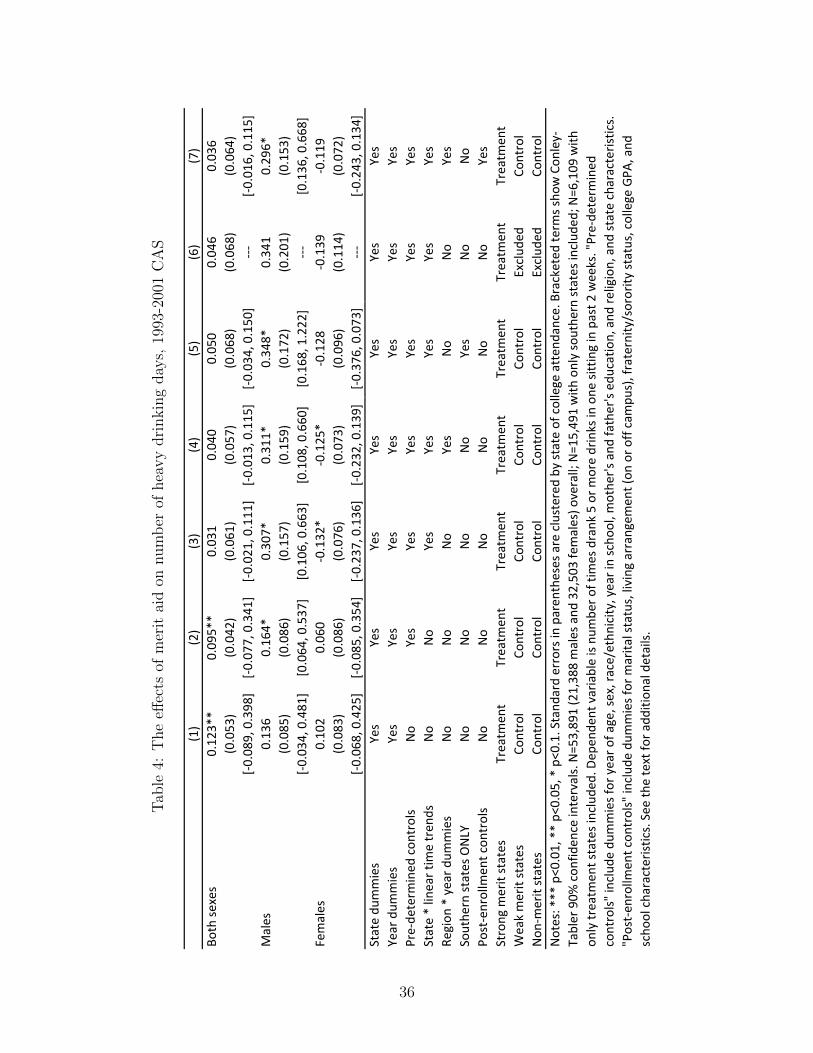
Tab

le4:

The

effec

tsof

mer

itai

don

num

ber

ofhea

vy

dri

nkin

gday

s,19

93-2

001

CA

S

(1)

(2)

(3)

(4)

(5)

(6)

(7)

Both se

xes

0.12

3**

0.09

5**

0.03

10.04

00.05

00.04

60.03

6(0.053

)(0.042

)(0.061

)(0.057

)(0.068

)(0.068

)(0.064

)[‐0

.089

, 0.398

][‐0

.077

, 0.341

][‐0

.021

, 0.111

][‐0

.013

, 0.115

][‐0

.034

, 0.150

]‐‐‐

[‐0.016

, 0.115

]Males

0.13

60.16

4*0.30

7*0.31

1*0.34

8*0.34

10.29

6*(0.085

)(0.086

)(0.157

)(0.159

)(0.172

)(0.201

)(0.153

)[‐0

.034

, 0.481

][0.064

, 0.537

][0.106

, 0.663

][0.108

, 0.660

][0.168

, 1.222

]‐‐‐

[0.136

, 0.668

]Females

0.10

20.06

0‐0.132

*‐0.125

*‐0.128

‐0.139

‐0.119

(0.083

)(0.086

)(0.076

)(0.073

)(0.096

)(0.114

)(0.072

)[‐0

.068

, 0.425

][‐0

.085

, 0.354

][‐0

.237

, 0.136

][‐0

.232

, 0.139

][‐0

.376

, 0.073

]‐‐‐

[‐0.243

, 0.134

]State du

mmies

Yes

Yes

Yes

Yes

Yes

Yes

Yes

Year dum

mies

Yes

Yes

Yes

Yes

Yes

Yes

Yes

Pre‐de

term

ined

 con

trols

No

Yes

Yes

Yes

Yes

Yes

Yes

State * linear tim

e tren

dsNo

No

Yes

Yes

Yes

Yes

Yes

Region

 * year d

ummies

No

No

No

Yes

No

No

Yes

Southe

rn states ONLY

No

No

No

No

Yes

No

No

Post‐enrollm

ent con

trols

No

No

No

No

No

No

Yes

Strong

 merit states

Treatm

ent

Treatm

ent

Treatm

ent

Treatm

ent

Treatm

ent

Treatm

ent

Treatm

ent

Weak merit states

Control

Control

Control

Control

Control

Exclud

edCo

ntrol

Non

‐merit states

Control

Control

Control

Control

Control

Exclud

edCo

ntrol

Notes: ***

 p<0.01, ** p<

0.05

, * p<0.1. Stand

ard errors in

 paren

theses are clustered

 by state of college atten

dance. Bracketed

 term

s sho

w Con

ley‐

Tabler 90%

 con

fiden

ce intervals. N=53,89

1 (21,38

8 males and

  32,50

3 females) o

verall; N=15,49

1 with

 only southe

rn states includ

ed; N

=6,109

 with

 on

ly treatm

ent states include

d. Dep

ende

nt variable is nu

mbe

r of tim

es drank

 5 or m

ore drinks in

 one

 sitting in past 2

 weeks. "Pre‐de

term

ined

 controls"

 includ

e du

mmies for year o

f age, sex, race/ethn

icity

, year in scho

ol, m

othe

r's and

 father's ed

ucation, and

 religion, and

 state characteristics. 

"Post‐en

rollm

ent con

trols" includ

e du

mmies for m

arita

l status, living

 arrangemen

t (on

 or o

ff campu

s), fraternity

/sorority

 status, college GPA

, and

 scho

ol characteristics. See

 the text fo

r add

ition

al details.

36

Table 5: The effects of merit aid on alternative drinking measures, 1993-2001 CAS

Both sexes 0.019 0.868 ‐0.007 0.031(0.011) (1.375) (0.017) (0.061)

Males ‐0.011 4.680** 0.012 0.307*(0.013) (2.125) (0.024) (0.157)

Females 0.037 ‐1.405 ‐0.018 ‐0.132*(0.022) (1.888) (0.028) (0.076)

Dependent variableDrank alcohol in past 

monthTotal number of drinks in 

past monthDrank 5+ drinks in past 2 

weeksNumber of days 5+ drinks 

in past 2 weeks

Notes: *** p<0.01, ** p<0.05, * p<0.1. Standard errors in parentheses are clustered by state of college attendance. Bracketed terms show Conley‐Tabler 90% confidence intervals. N=53,891 (21,388 males and 32,503 females). All models include controls for state and year dummies, pre‐determined controls, and state time trends. "Pre‐determined controls" include dummies for year of age, sex, race/ethnicity, year in school, mother's and father's education, and religion, and state characteristics.

Table 6: The effects of merit aid on pre-college student characteristics, 1993-2001 CAS

Both sexes ‐0.026 0.024 0.041* ‐0.010 ‐0.026** ‐0.087(0.027) (0.091) (0.023) (0.022) (0.011) (0.394)

Males ‐‐‐ ‐0.062 0.022 ‐0.013 ‐0.030* 0.042(0.063) (0.036) (0.018) (0.016) (0.616)

Females ‐‐‐ 0.077 0.046** ‐0.008 ‐0.019 ‐0.143(0.128) (0.021) (0.028) (0.015) (0.326)

Dependent variable

Sex=Female Age (in years) Race=WhiteFather attended 

collegeMother attended 

collegeHigh‐school drinking

Notes: *** p<0.01, ** p<0.05, * p<0.1. Standard errors in parentheses are clustered by state of college attendance. N=53,891 (21,388 males and 32,503 females). All models include controls for state and year dummies, pre‐determined controls, and state time trends. See Table 4 for additional details. "High‐school drinking" is measured as the reported number of times per month the student drank alcohol while in high school.

37

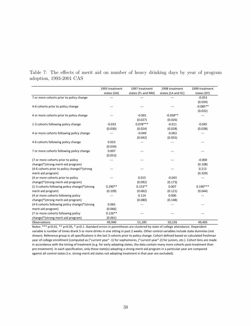
Table 7: The effects of merit aid on number of heavy drinking days by year of programadoption, 1993-2001 CAS

7 or more cohorts prior to policy change ‐‐‐ ‐‐‐ ‐‐‐ ‐0.053

(0.034)

4‐6 cohorts prior to policy change ‐‐‐ ‐‐‐ ‐‐‐ ‐0.085**

(0.032)

4 or more cohorts prior to policy change ‐‐‐ ‐0.001 ‐0.058** ‐‐‐

(0.027) (0.026)

1‐3 cohorts following policy change ‐0.033 0.078*** ‐0.011 ‐0.045

(0.030) (0.024) (0.028) (0.038)

4 or more cohorts following policy change ‐‐‐ ‐0.049 ‐0.063 ‐‐‐

(0.042) (0.055)

4‐6 cohorts following policy change 0.053 ‐‐‐ ‐‐‐ ‐‐‐

(0.034)

7 or more cohorts following policy change 0.007 ‐‐‐ ‐‐‐ ‐‐‐

(0.053)

‐‐‐ ‐‐‐ ‐‐‐ ‐0.000

(0.108)

‐‐‐ ‐‐‐ ‐‐‐ 0.213

(0.329)

‐‐‐ 0.015 ‐0.043 ‐‐‐

(0.092) (0.173)

0.290** 0.153** 0.007 0.190***

(0.109) (0.062) (0.121) (0.044)

‐‐‐ 0.114 0.000 ‐‐‐

(0.080) (0.148)

0.065 ‐‐‐ ‐‐‐ ‐‐‐

(0.066)

0.126** ‐‐‐ ‐‐‐ ‐‐‐

(0.061)

Observations 49,940 51,185 50,226 49,405

Notes: *** p<0.01, ** p<0.05, * p<0.1. Standard errors in parentheses are clustered by state of college attendance. Dependent 

variable is number of times drank 5 or more drinks in one sitting in past 2 weeks. Other control variables include state dummies (not 

shown). Reference group in all specifications is the last 3 cohorts prior to policy change. Cohort defined based on calculated freshman 

year of college enrollment (computed as ("current year" ‐1) for sophomores, ("current year"‐2) for juniors, etc.). Cohort bins are made 

in accordance with the timing of treatment (e.g. for early adopting states, the data contain many more cohorts post‐treatment than 

pre‐treatment). In each specification, only those state(s) adopting a strong merit‐aid program in a particular year are compared 

against all control states (i.e. strong‐merit aid states not adopting treatment in that year are excluded).

1993 treatment 

states (GA)

1997 treatment 

states (FL and NM)

1998 treatment 

states (LA and SC)

1999 treatment 

states (KY)

(7 or more cohorts prior to policy 

change)*(strong merit‐aid program)

(4‐6 cohorts prior to policy change)*(strong 

merit‐aid program)

(4 or more cohorts prior to policy 

change)*(strong merit‐aid program)

(1‐3 cohorts following policy change)*(strong 

merit‐aid program)

(4 or more cohorts following policy 

change)*(strong merit‐aid program)

(4‐6 cohorts following policy change)*(strong 

merit‐aid program)

(7 or more cohorts following policy 

change)*(strong merit‐aid program)

38

Tab

le8:

The

effec

tsof

mer

itai

don

hea

vy

dri

nkin

gby

pre

-col

lege

studen

tch

arac

teri

stic

s,19

93-2

001

CA

S

Both se

xes

0.07

10.02

60.03

30.17

8*0.29

6**

‐0.144

0.17

8‐0.047

(0.078

)(0.078

)(0.134

)(0.096

)(0.114

)(0.121

)(0.110

)(0.120

)N=11,45

1N=42,44

0N=26,29

7N=27,59

4N=18,07

7N=35,81

4N=15,93

8N=37,95

3Males

0.12

30.35

9*0.15

20.74

1***

0.57

8**

0.10

80.40

10.26

4(0.137

)(0.189

)(0.315

)(0.227

)(0.242

)(0.171

)(0.367

)(0.169

)N=4,407

N=16,98

1N=9,599

N=11,78

9N=7,112

N=14,27

6N=5,856

N=15,53

2Females

0.04

3‐0.183

0.00

2‐0.206

**0.13

0‐0.297

**0.07

3‐0.258

**(0.064

)(0.114

)(0.209

)(0.078

)(0.130

)(0.132

)(0.146

)(0.119

)N=7,044

N=25,45

9N=16,69

8N=15,80

5N=10,96

5N=21,53

8N=10,08

2N=22,42

1

By father's ed

ucation

Notes: ***

 p<0.01, ** p<

0.05

, * p<0.1. Stand

ard errors in

 paren

theses are clustered

 by state of college atten

dance. Dep

ende

nt variable is nu

mbe

r of tim

es drank

 5 or m

ore 

drinks in

 one

 sitting in past 2

 weeks. A

ll  mod

els include

 con

trols for state and year dum

mies, pre‐determined

 con

trols, and

 state tim

e tren

ds. See

 Table 4 fo

r add

ition

al details.

Non

‐white

White

Less th

an 21

21 and

 older

Mothe

r did not 

attend

Mothe

r did atten

dFather did not 

attend

Father did atten

d

By ra

ceBy

 age

By m

othe

r's edu

catio

n

39

Tab

le9:

The

effec

tsof

mer

itai

don

hea

vy

dri

nkin

gby

pos

t-en

rollm

ent

studen

tch

arac

teri

stic

s,19

93-2

001

CA

S

GPA

<2.7

2.7<=G

PA<3.4

GPA

>=3.4

Non

‐greek

Greek

Private

Public

Both se

xes

‐0.132

0.31

1***

0.00

90.02

5‐0.280

‐0.155

***

0.07

2(0.275

)(0.108

)(0.076

)(0.052

)(0.229

)(0.044

)(0.063

)N=7,253

N=17,74

5N=28,24

6N=46,24

4N=7,647

N=17,17

0N=36,72

1Males

‐0.446

0.66

5**

0.49

1***

0.30

6***

‐0.351

0.09

70.32

6*(0.388

)(0.298

)(0.131

)(0.108

)(0.628

)(0.078

)(0.171

)N=3,457

N=7,563

N=10,13

3N=18,17

4N=3,214

N=6,290

N=15,09

8Females

0.15

60.09

8‐0.247

*‐0.145

**‐0.170

‐0.239

***

‐0.092

(0.284

)(0.138

)(0.133

)(0.064

)(0.219

)(0.046

)(0.100

)N=3,796

N=10,18

2N=18,11

3N=28,07

0N=4,433

N=10,88

0N=21,62

3Notes: ***

 p<0.01, ** p<

0.05

, * p<0.1. Stand

ard errors in

 paren

theses are clustered

 by state of college atten

dance. Dep

ende

nt variable is nu

mbe

r of tim

es 

drank 5 or m

ore drinks in

 one

 sitting in past 2

 weeks. A

ll mod

els include

 con

trols for state and year dum

mies, pre‐determined

 con

trols, and

 state tim

e tren

ds. See

 Table 4 fo

r add

ition

al details.

By fraternity/sorority

 status

By institu

tion type

By grade

 point average (G

PA)

40

App

endix

Tab

le1:

The

effec

tsof

mer

itai

don

hea

vy

dri

nkin

gday

sex

cludin

gw

eak-m

erit

stat

es,

1993

-200

1C

AS

(1)

(2)

(3)

(4)

(5)

(6)

Both se

xes

0.11

0*0.10

0**

0.03

40.04

00.04

50.01

7(0.058

)(0.047

)(0.063

)(0.062

)(0.068

)(0.071

)[‐0

.182

, 0.487

][‐0

.144

, 0.431

][‐0

.051

, 0.142

][‐0

.047

, 0.138

][‐0

.086

, 0.206

][‐0

.085

, 0.119

]Males

0.12

00.19

2*0.35

7**

0.35

9**

0.35

1*0.31

5*(0.094

)(0.094

)(0.168

)(0.172

)(0.178

)(0.159

)[‐0

.101

, 0.598

][0.050

, 0.764

][0.077

, 0.786

][0.062

, 0.764

][‐0

.191

, 0.794

][0.085

, 0.765

]Females

0.09

40.05

0‐0.172

**‐0.170

**‐0.134

‐0.176

**(0.087

)(0.087

)(0.075

)(0.075

)(0.089

)(0.083

)[‐0

.149

, 0.522

][‐0

.192

, 0.426

][‐0

.315

, 0.176

][‐0

.309

, 0.168

][‐0

.256

, 0.434

][‐0

.324

, 0.119

]State du

mmies

Yes

Yes

Yes

Yes

Yes

Yes

Year dum

mies

Yes

Yes

Yes

Yes

Yes

Yes

Pre‐de

term

ined

 con

trols

No

Yes

Yes

Yes

Yes

Yes

State * linear  tim

e tren

dsNo

No

Yes

Yes

Yes

Yes

Region

 * year d

ummies

No

No

No

Yes

No

Yes

Southe

rn states ONLY

No

No

No

No

Yes

No

Post‐enrollm

ent con

trols

No

No

No

No

No

Yes

Strong

 merit states

Treatm

ent

Treatm

ent

Treatm

ent

Treatm

ent

Treatm

ent

Treatm

ent

Weak merit states

Exclud

edExclud

edExclud

edExclud

edExclud

edExclud

edNon

‐merit states

Control

Control

Control

Control

Control

Control

Notes: ***

 p<0.01, ** p<

0.05

, * p<0.1. Stand

ard errors in

 paren

theses are clustered

 by state of college atten

dance. Bracketed

 term

s sho

w Con

ley‐Tabler 90%

 con

fiden

ce intervals. N=29,65

1 (11,96

5 males and

 17,68

6 females) o

verall;  N=12,88

8 with

 only 

southe

rn states includ

ed. D

epen

dent variable is nu

mbe

r of tim

es drank

 5 or m

ore drinks in

 one

 sitting in past 2

 weeks. "Pre‐

determ

ined

 con

trols" includ

e du

mmies for year o

f age, sex, race/ethn

icity

, year in scho

ol, m

othe

r's and

 father's ed

ucation, and

 religion, and

 state characteristics. "Po

st‐enrollm

ent con

trols" includ

e  du

mmies for m

arita

l status, living

 arrangemen

t (on

 or o

ff campu

s), fraternity

/sorority

 status, college GPA

, and

 scho

ol characteristics. See

 the text fo

r add

ition

al details.

41

App

endix

Tab

le2:

The

effec

tsof

mer

itai

don

tota

lnum

ber

ofdri

nks,

1993

-200

1C

AS

(1)

(2)

(3)

(4)

(5)

(6)

(7)

Both se

xes

2.11

92.23

00.86

80.82

91.20

71.62

80.65

8(1.997

)(1.854

)(1.375

)(1.292

)(1.467

)(1.099

)(1.328

)[‐1

.791

, 8.750

][‐1

.185

, 8.648

][0.032

, 2.196

][‐0

.021

, 2.055

][‐0

.195

, 2.781

]‐‐‐

[‐0.205

, 1.944

]Males

2.29

53.58

64.68

0**

4.10

1*4.57

35.87

1*3.71

8**

(2.315

)(2.496

)(2.125

)(2.156

)(2.674

)(2.810

)(1.710

)[‐0

.250

, 10.13

7][2.320

, 11.62

0][0.175

, 13.31

6][‐0

.495

, 11.93

0][‐0

.437

, 21.28

4]‐‐‐

[0.023

, 11.93

5]Females

1.80

71.54

8‐1.405

‐1.292

‐0.854

‐1.029

‐1.293

(2.095

)(2.131

)(1.888

)(1.810

)(2.166

)(1.856

)(1.768

)[‐1

.217

, 9.063

][‐1

.263

, 8.841

][‐3

.364

, 5.127

][‐3

.546

, 5.160

][‐6

.435

, 3.919

]‐‐‐

[‐0.240

, 5.019

]State du

mmies

Yes

Yes

Yes

Yes

Yes

Yes

Yes

Year dum

mies

Yes

Yes

Yes

Yes

Yes

Yes

Yes

Pre‐de

term

ined

 con

trols

No

Yes

Yes

Yes

Yes

Yes

Yes

State * linear tim

e tren

dsNo

No

Yes

Yes

Yes

Yes

Yes

Region

 * year d

ummies

No

No

No

Yes

No

No

Yes

Southe

rn states ONLY

No

No

No

No

Yes

No

No

Post‐enrollm

ent con

trols

No

No

No

No

No

No

Yes

Strong

 merit states

Treatm

ent

Treatm

ent

Treatm

ent

Treatm

ent

Treatm

ent

Treatm

ent

Treatm

ent

Weak merit states

Control

Control

Control

Control

Control

Exclud

edCo

ntrol

Non

‐merit states

Control

Control

Control

Control

Control

Exclud

edCo

ntrol

Notes: ***

 p<0.01, ** p<

0.05

, * p<0.1. Stand

ard errors in

 paren

theses are clustered

 by state of college atten

dance. Bracketed

 term

s sho

w Con

ley‐

Tabler 90%

 con

fiden

ce intervals. N=53,89

1 (21,38

8 males  and

 32,50

3 females) o

verall; N=15,49

1 with

 only southe

rn states includ

ed; N

=6,109

 with

 on

ly treatm

ent states include

d. Dep

ende

nt variable is total num

ber o

f alcoh

olic drin

ks in

 past m

onth. "Pre‐de

term

ined

 con

trols" includ

e du

mmies 

for y

ear o

f age, sex, race/ethn

icity

, year in scho

ol, m

othe

r's and

 father's ed

ucation, and

 religion, and

 state characteristics. "Po

st‐enrollm

ent 

controls"

 includ

e du

mmies for m

arita

l status, living

 arrangemen

t (on

 or o

ff campu

s), fraternity

/sorority

 status, college GPA

, and

 scho

ol 

characteristics. See

 the text fo

r add

ition

al details.

42