The Effects of Universal Free Lunch Provision onStudent Achievement: Evidence from South Korea

Yoonjung Kim ∗

October 19, 2021

Click for Latest Version

Abstract

This paper examines the impact of the Universal Free Lunch Program (UFLP)on student achievement in South Korea. I leverage the staggered rollout ofthe UFLP across South Korean provinces and employ difference-in-differencesstrategies to estimate the causal effects of the program. Taking advantage ofrich school-level data, I find that providing a free lunch to all students leads toimprovements in academic achievement on average. I also test for heterogeneouseffects and find that the benefits of the UFLP appear universally across differentbaseline participation rates in the means-tested lunch subsidy. After exploringnumerous potential mechanisms including changes in school lunch participation,I find suggestive evidence of the increased participation in and expenditureson the after-school programs that are not free. These results suggest thatparents used the saved lunch fees for educational investment and highlight theimportance of mental accounting.

Keywords: school lunch, test scores, educational policyJEL Codes: H42, H52, I38

∗Kim: Department of Economics, University of California, Irvine (e-mail: yoonjunk@uci.edu). I owe manythanks to Matthew Freedman, Meera Mahadevan, Damon Clark, and Vellore Arthi for their invaluable help incompleting this project. I thank Aria Golestani, Tejaswi Velayudhan, Yingying Dong, Yingying Lee, DavidNeumark, Emily Beam, Marrianne Bitler, Daniel Lee, Hoyt Bleakley, Janet Currie, Ashley Craig, DavidMartin, Alex Eble, Felipe Barrera-Osorio, Robert Wassmer, Wesley Yin, and Chloe East for constructivediscussion. I appreciate the feedback of conference audiences and seminar participants at the Associationfor Mentoring and Inclusion in Economics, WEAI, NEUDC, APPAM, SEA, ACLEC, and the University ofCalifornia, Irvine. I thank the Department of Economics at UC Irvine for research funding. I am gratefulto the Ministry of Education of South Korea for granting access to the administrative data.

1

1 Introduction

Despite the differences in culture, wealth, and academic policy across nations, school meals

are a crucial source of nutrition intake for many students: 300 million children in 85 countries

participate in large-scale school meal programs worldwide (Global Child Nutrition Founda-

tion 2021). Many of these countries also provide school meal subsidies. South Korea’s

Ministry of Education reports that in 2016, the Universal Free Lunch Program (UFLP) cost

2.8 billion USD, or 0.2 percent of GDP (Ministry of Education 2021). Still, proper evaluation

requires weighing the program’s cost against its social welfare maximizing benefits. School

meals are a type of schooling input, as students receive school meals in classrooms or on

school grounds. Increasing schooling inputs positively relates to better academic achieve-

ment, higher earnings (Murnane et al. 2000; Currie and Thomas 2001; Heckman and Vytacil

2001; Dougherty 2003; Heckman et al. 2006; Deming 2009; Chetty et al., 2011) and other

important later life outcomes including health (Lleras-Muney 2005; Eide, Showalter, and

Goldhaber 2010; Weinstein and Skinner 2010; Clark and Royer 2013).

This paper examines the impacts of South Korea’s Universal Free Lunch Program (UFLP)

on students’ academic achievement. By leveraging the staggered implementation and rich

administrative data, I estimate the intent-to-treat effect of the UFLP, and find that the

program reduced underachievement by 13 percent and improved test scores by 0.06 standard

deviations. I explore potential channels and find evidence that parents react to the additional

disposable income (saved lunch fees, approximately $700 per year) by allocating it towards

educational investment. I find increased participation in and spending on academic after-

school programs, which are generally not free. The UFLP’s impacts are robust to sparser or

more saturated specifications and the inclusion of province characteristics.1 Moreover, these

effects are found universally across different baseline participation rates in the means-tested

lunch subsidy for both average standardized scores and the percentage of underachieving

1These checks are discussed in detail in section 6, including the DIDM estimates of de Chaisemartin andD’Haultfoeuille (2020) and the related results.

2

students. These results are consistent with the implication of the UFLP as an in-kind transfer

to relatively higher income families, since lower income families had access to means-tested

lunch subsidies prior to the UFLP.

There are several reasons why the UFLP and the South Korean context are worth inves-

tigating. First, the UFLP reached all students from elementary to high school without any

kinds of means-testing, unlike other meal programs. For example, the Midday meal program

in India is only for public primary school students, and the Community Eligibility Provision

(CEP) in the US targets schools with a relatively high percentage of students eligible for free

or reduced-price lunches. Second, the UFLP is large, making up approximately 5 percent

of total local government educational expenditures. Given the size of the program, under-

standing the impacts of the UFLP helps justify its existence, especially when an increase

in enrollment and school lunch participation is relatively less likely in the South Korean

setting (OECD 2017, 2021a, 2021b).2 Third, South Korea provides a testing ground for the

effects of universal meal provision when means-tested lunch subsidy is already in place. As

most countries provide school meal subsidies for students with relatively low family incomes

(OECD 2017), this study can provide pertinent policy implications for many other countries

that might consider universal school meal provision.

This paper contributes to two distinct strands of literature. The first is studies that

focus on the impact of school meal subsidies and their effect on various outcomes, including

health (Bhattacharya et al. 2006; Schanzenbach 2009; Gundersen, Kreider, and Pepper 2012;

Berry et al. 2020) and academic achievement (Hinrichs 2010; Leos-Urbel et al. 2013; Frisvold

2015; Schwartz and Rothbart 2020; Chakraborty and Jayaraman 2019; Gordanier et al. 2020;

Ruffini 2020). While this literature is heavily based on evidence from the US, this paper

can add to the generalizability of findings in the literature. This paper finds improvements

in standardized scores of 0.05 to 0.11 standard deviations due to the implementation of

the UFLP. The magnitude of improved standardized scores is comparable to the estimated

2School lunch participation had been close to 100 percent before the UFLP. See section 5.1.1 for moredetails.

3

effects found in Chakraborty and Jayaraman (2019) in India, and Schwartz and Rothbart

(2019), Ruffini (2021) and Gordanier et al. (2020) in the US. Moreover, my results suggest

that the program is relatively cost-effective compared to many other educational programs

in the US setting, including a 10 percent increase in spending and class size reduction (Yeh,

2010).

The second strand studies household consumption decisions. The estimates imply that

parents reallocate the additional disposable income towards the students. The estimates

imply that students on average participate in 0.4 more after-school programs throughout the

year, or 5 months’ worth of participation in one program. Back-of-the-envelope estimates

of the cost of this increased academic after-school program participation suggest 12 to 25

percent of the saved lunch fee is spent on students’ education.3 Empirical results examining

the effects of providing benefits earmarked for children provide insights that parents are

likely to spend the benefit on children (Lundberg, Pollak and Wales 1997; Hener 2017; Jones

et al. 2019) by increasing spending on education and non-food items, although (partial)

crowd-out in food spending is observed (Chakraborty and Jayaraman 2020; Handbury and

Moshary 2020).4 This increase in spending on children can be linked to the mental accounting

framework (Thaler 1990, 1998, and 1999). I find suggestive evidence of an increase in the

academic after-school program participation due to the implementation of the UFLP, which

indicates increased spending on education.5

More broadly, this paper also relates to the literature that studies the impacts of pub-

lic assistance programs on children’s outcomes, including academic achievement. Because

changes in school lunch participation in the South Korean context are unlikely, as I show

in panel (a) of figure 1, the UFLP operates as an in-kind transfer. For example, Milligan

and Stabile (2011) and Dahl and Lochner (2012) find that tax benefits improve children’s

3Unlike in the US, these programs are generally not free.4Lundberg, Pollak and Wales (1997) and Kenney (2008) also point out that this phenomenon is prone

to be greater if the child benefits are controlled by the mother. Before the UFLP, school lunch fees weregenerally paid by mothers as shown by anecdotal evidence (Ryu et al. 2011) and research on householdfinancial management (Lee and Yang 2008).

5I discuss the more related studies in appendix section A.

4

academic achievement and various health measures. Akee et al. (2010) also find that an

exogenous increase in household income from transfer payments led to higher education

attainment for the children in affected households.

This paper proceeds as follows. In section 2, I summarize the general information re-

garding the South Korean school system alongside the characteristics of the Universal Lunch

Program. Section 3 describes the data. I discuss the estimation strategies in section 4, and

present the results in section 5. I provide robustness checks and discuss the heterogeneous

effects across baseline participation rate in the means-tested school subsidy in section 6. I

address potential mechanisms in section 7, and conclude in section 8.

2 Background and Institutional Context

The UFLP replaced the already existing means-tested school lunch subsidy, but the timing of

implementation or expansion of the ULFP was staggered due to the provincial governments’

budgetary concerns.67 The rollout information for all provinces is summarized in appendix

tables A.1 to A. 4. Due to the staggered rollout procedures, in many cases the UFLP treated

only some of the students within a school.

From the parents’ perspective, lunch fees make up a large portion of education expenses.

Depending on school levels, expenses include slightly different categories8. Starting with the

UFLP, the government also added other policies to reduce the cost of education, including

subsidies for school uniforms and textbooks. Still, these policies did not coincide with the

timing of the UFLP implementation, and most of them did not occur until the end of the

6Students with family incomes less than 60 percent of the median income (considering family asset value)were eligible for the means-tested school lunch subsidy before the UFLP. The exact threshold for the eligibilitycan be slightly different in each province (Ministry of Education 2021).

7It is impossible to obtain the exact breakdown of the UFLP’s budget, but on average, the provincialeducation budget in South Korea combines 60 percent of the Ministry of Education’s budget (direct centralgovernment expenditures) and 40 percent of the provincial government’s budget (Ministry of Education2021). But approximately 80 percent of the provincial government’s budget is supplemented by the centralgovernment (Hyeon and Shin 2016).

8These categories include entrance fees, tuition, operational support fees, school meal fees, and schooluniform costs, but depending on the school level, some might not be included. For example, elementaryschools almost never require a school uniform.

5

sample period of this study. This ensures that the estimated effects of the UFLP are not

confounded with the effects of other educational subsidies.

Parents’ payments to the schools can be sticky, especially since there is a widely adopted

and convenient payment system which has applied to all fees that the parents pay to the

schools since the late 1990s (Jeong 1997; Eum 1997). Through this system, parents provide

the account number of one of their checking accounts to their children’s schools, and give

authorization to withdraw the deposit if needed (KFTC 2021). Since both school lunch and

after-school program fees are processed through the same account, parents are likely to apply

mental accounting to the fees, as these fees in total would be easily grouped together.

In panel (a) of figure 1, I plot the average value of students’ participation in school lunch

programs and the share of students who benefit from school lunch subsidies. This figure

implies that the average participation rate in the school lunch programs was very close to

one regardless of the UFLP implementation. In panel (b) of figure 1, I plot the average

value of parents’ and governments’ contribution relative to the total yearly budget for school

meals. A reduction in the parents’ shares in contrast to the increase in the government’s

contribution is evident.

A reduction in parents’ contributions leads to increased disposable income for families

with school-aged children by saving school lunch expenses. Still, the extent of this increase

differs by family income and participation in the means-tested school meal subsidy. If families

were already participating in the means-tested lunch subsidy before the UFLP started, they

would not experience an increase in disposable income.9 The families ineligible for the

means-tested lunch subsidy due to relatively higher income would experience an increase in

disposable income due to the UFLP by saving lunch fees, which are approximately $600-$720

per year for each student. General details about the school system in South Korea can be

found in Appendix section B.

9There are no official estimates regarding the take-up of the means-tested lunch subsidy. Yu, Lim andKelly (2019) find suggestive evidence that the stigma can affect the take-up.

6

3 Data

3.1 EduData Service System Data

I use restricted data provided by EduData Service System (EDSS) from 2009 to 2016. This

data sampled 70 percent of all schools in South Korea and contains various information

about each school, such as the number of students, the number of teachers, school facilities,

and school food expenditures. This data also contains information regarding the National

Assessment of Educational Achievement (NAEA) exam for Korean, math, and English.10 11

The sample consists of 20,310 school-by-year observations, and approximately 41 percent

of school-by-year observations was either fully or partially treated during the sample period.

Column (1) of table 1 reports the summary statistics of the academic achievement outcomes

of interest, school characteristics, and variables related to school meal provision.

EDSS data has abundant information regarding school meal provision. In the South

Korean context, most of the students get lunch from schools. Regardless of the treatment

status, almost all students receive lunch from school. The share of students who receive

school meal subsidies is roughly 23 percentage points higher in the treated schools. This

share is roughly 0.5 among the treated schools, which falls short of the maximum value

mostly due to the staggered adoption of the program even within a school. Per student

meal expenditure is slightly greater for the treated schools, but this is likely due to inflation

over the years and high schools generally having higher per student meal expenditures. By

comparing the share of parents’ contribution and the governments’ contribution, the main

source of funding for the school meals is parents among the pre-treatment observations and

the government among the post-treatment observations. This change of source of funding is

discussed in more detail in section 5.1.1.

10These test results are used to gauge the quality of school education, and to make sure that students atthe lower tail of the score distribution follow the curriculum. Comparable exams are the National Assessmentof Educational Progress (NAEP) in the US or the Standard Assessment Task in the UK.

11After 2016, the Ministry of Education stopped the comprehensive tests and sampled only three percentof the schools. The scores after 2016 are not available from the EDSS.

7

To investigate the changes in education expenditure due to the UFLP, I use the EDSS data

to estimate the effects of the UFLP on after-school program participation and expenditures.

EDSS data has information on how many students participated in both academic and non-

academic after-school programs, and I use the average number of programs in which students

participated in each school as an outcome to examine this potential underlying mechanism.

In South Korea, most of the after-school programs are not free and parents have to make

payments for the students to participate. Thus, increased after-school program participation

implies increased expenditure.

Province Characteristics. The bottom panel of table 1 reports the province character-

istics. I report the two financial independence indices that Statistics Korea publishes yearly.12

The provincial government’s financial independence is emphasized by many of the Ministry

of Education’s government officials as a crucial determinant of the UFLP implementation

timing. Provinces with higher financial capacity, which is associated with a higher level of

financial independence indices, were more likely to adopt the UFLP earlier. I also gauged

superintendents’ support for the UFLP using interviews and their election promises. I ob-

tained the province-level unemployment rate series from the Korean Statistical Information

Service (KOSIS).13 Since the eligibility for the means-tested lunch subsidy largely depends

on household income, the regional unemployment rate can affect the baseline participation

in the means-tested subsidy, which can change the UFLP’s impact.

3.2 Private Education Expenditures Survey

In this subsection, I describe the Private Education Expenditures Survey data (PES), which

I utilize to investigate underlying mechanisms. The PES contains student-by-year repeated

cross-section data and has information on approximately 55,000 middle (22,000) and high

school (33,000) students each year. The parents and the teachers of the students answer

12For more information, visit https://www.index.go.kr/potal/main/EachDtlPageDetail.do?idx cd=

2857 and https://www.index.go.kr/potal/main/EachDtlPageDetail.do?idx cd=2458.13See https://kosis.kr/statHtml/statHtml.do?orgId=101&tblId=INH 1DA7104S&conn path=I3 for

more information.

8

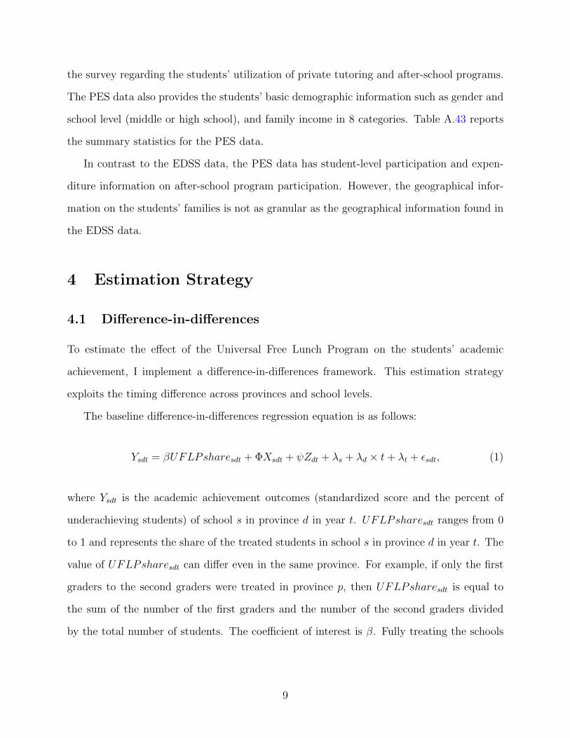
the survey regarding the students’ utilization of private tutoring and after-school programs.

The PES data also provides the students’ basic demographic information such as gender and

school level (middle or high school), and family income in 8 categories. Table A.43 reports

the summary statistics for the PES data.

In contrast to the EDSS data, the PES data has student-level participation and expen-

diture information on after-school program participation. However, the geographical infor-

mation on the students’ families is not as granular as the geographical information found in

the EDSS data.

4 Estimation Strategy

4.1 Difference-in-differences

To estimate the effect of the Universal Free Lunch Program on the students’ academic

achievement, I implement a difference-in-differences framework. This estimation strategy

exploits the timing difference across provinces and school levels.

The baseline difference-in-differences regression equation is as follows:

Ysdt = βUFLPsharesdt + ΦXsdt + ψZdt + λs + λd × t+ λt + εsdt, (1)

where Ysdt is the academic achievement outcomes (standardized score and the percent of

underachieving students) of school s in province d in year t. UFLPsharesdt ranges from 0

to 1 and represents the share of the treated students in school s in province d in year t. The

value of UFLPsharesdt can differ even in the same province. For example, if only the first

graders to the second graders were treated in province p, then UFLPsharesdt is equal to

the sum of the number of the first graders and the number of the second graders divided

by the total number of students. The coefficient of interest is β. Fully treating the schools

9

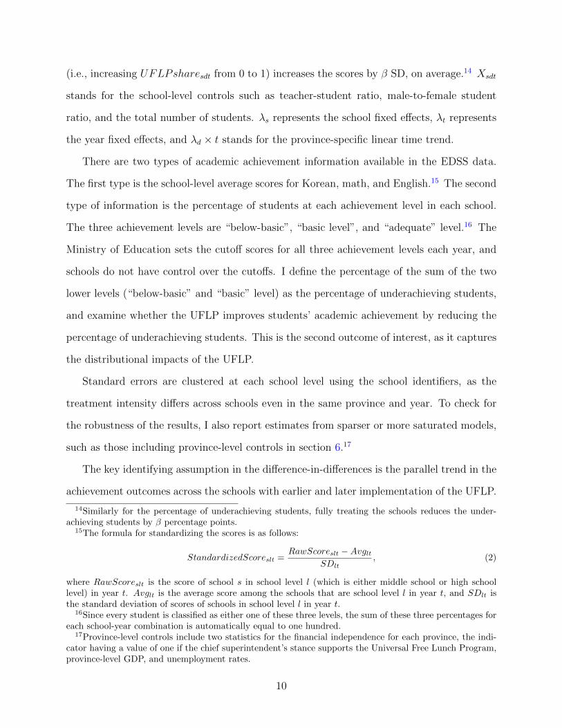
(i.e., increasing UFLPsharesdt from 0 to 1) increases the scores by β SD, on average.14 Xsdt

stands for the school-level controls such as teacher-student ratio, male-to-female student

ratio, and the total number of students. λs represents the school fixed effects, λt represents

the year fixed effects, and λd × t stands for the province-specific linear time trend.

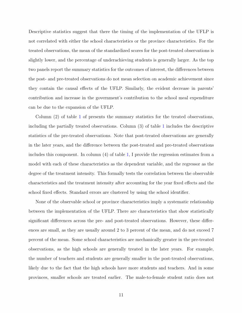
There are two types of academic achievement information available in the EDSS data.

The first type is the school-level average scores for Korean, math, and English.15 The second

type of information is the percentage of students at each achievement level in each school.

The three achievement levels are “below-basic”, “basic level”, and “adequate” level.16 The

Ministry of Education sets the cutoff scores for all three achievement levels each year, and

schools do not have control over the cutoffs. I define the percentage of the sum of the two

lower levels (“below-basic” and “basic” level) as the percentage of underachieving students,

and examine whether the UFLP improves students’ academic achievement by reducing the

percentage of underachieving students. This is the second outcome of interest, as it captures

the distributional impacts of the UFLP.

Standard errors are clustered at each school level using the school identifiers, as the

treatment intensity differs across schools even in the same province and year. To check for

the robustness of the results, I also report estimates from sparser or more saturated models,

such as those including province-level controls in section 6.17

The key identifying assumption in the difference-in-differences is the parallel trend in the

achievement outcomes across the schools with earlier and later implementation of the UFLP.

14Similarly for the percentage of underachieving students, fully treating the schools reduces the under-achieving students by β percentage points.

15The formula for standardizing the scores is as follows:

StandardizedScoreslt =RawScoreslt −Avglt

SDlt, (2)

where RawScoreslt is the score of school s in school level l (which is either middle school or high schoollevel) in year t. Avglt is the average score among the schools that are school level l in year t, and SDlt isthe standard deviation of scores of schools in school level l in year t.

16Since every student is classified as either one of these three levels, the sum of these three percentages foreach school-year combination is automatically equal to one hundred.

17Province-level controls include two statistics for the financial independence for each province, the indi-cator having a value of one if the chief superintendent’s stance supports the Universal Free Lunch Program,province-level GDP, and unemployment rates.

10

Descriptive statistics suggest that there the timing of the implementation of the UFLP is

not correlated with either the school characteristics or the province characteristics. For the

treated observations, the mean of the standardized scores for the post-treated observations is

slightly lower, and the percentage of underachieving students is generally larger. As the top

two panels report the summary statistics for the outcomes of interest, the differences between

the post- and pre-treated observations do not mean selection on academic achievement since

they contain the causal effects of the UFLP. Similarly, the evident decrease in parents’

contribution and increase in the government’s contribution to the school meal expenditure

can be due to the expansion of the UFLP.

Column (2) of table 1 of presents the summary statistics for the treated observations,

including the partially treated observations. Column (3) of table 1 includes the descriptive

statistics of the pre-treated observations. Note that post-treated observations are generally

in the later years, and the difference between the post-treated and pre-treated observations

includes this component. In column (4) of table 1, I provide the regression estimates from a

model with each of these characteristics as the dependent variable, and the regressor as the

degree of the treatment intensity. This formally tests the correlation between the observable

characteristics and the treatment intensity after accounting for the year fixed effects and the

school fixed effects. Standard errors are clustered by using the school identifier.

None of the observable school or province characteristics imply a systematic relationship

between the implementation of the UFLP. There are characteristics that show statistically

significant differences across the pre- and post-treated observations. However, these differ-

ences are small, as they are usually around 2 to 3 percent of the mean, and do not exceed 7

percent of the mean. Some school characteristics are mechanically greater in the pre-treated

observations, as the high schools are generally treated in the later years. For example,

the number of teachers and students are generally smaller in the post-treated observations,

likely due to the fact that the high schools have more students and teachers. And in some

provinces, smaller schools are treated earlier. The male-to-female student ratio does not

11

differ between the pre-treated and post-treated observations, which implies that the UFLP

does not favor or target schools based on students’ gender. The number of students who

transfer in and transfer out also remained stable, which suggests a low chance of selection

into treatment. Still, I include school characteristics in all specifications, and also include

province characteristics for robustness checks.

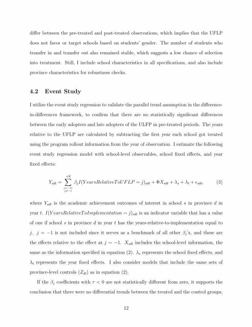
4.2 Event Study

I utilize the event study regression to validate the parallel trend assumption in the difference-

in-differences framework, to confirm that there are no statistically significant differences

between the early adopters and late adopters of the ULFP in pre-treated periods. The years

relative to the UFLP are calculated by subtracting the first year each school got treated

using the program rollout information from the year of observation. I estimate the following

event study regression model with school-level observables, school fixed effects, and year

fixed effects:

Ysdt =+9∑

j=−11j 6=−1

βjI(Y earsRelativeToUFLP = j)sdt + ΦXsdt + λs + λt + εsdt, (3)

where Ysdt is the academic achievement outcomes of interest in school s in province d in

year t. I(Y earsRelativeToImplementation = j)sdt is an indicator variable that has a value

of one if school s in province d in year t has the years-relative-to-implementation equal to

j. j = −1 is not included since it serves as a benchmark of all other βj’s, and these are

the effects relative to the effect at j = −1. Xsdt includes the school-level information, the

same as the information specified in equation (2). λs represents the school fixed effects, and

λt represents the year fixed effects. I also consider models that include the same sets of

province-level controls (Zdt) as in equation (2).

If the βj coefficients with τ < 0 are not statistically different from zero, it supports the

conclusion that there were no differential trends between the treated and the control groups,

12

conditional on the control variables included in equation (3). I also report the statistical test

results for the null hypothesis that the βj’s in the pre-periods are jointly equal to zero.

In appendix section C, I discuss the instrumental variable regression model, which uses

the UFLP rollout information as an instrument for the share of subsidized students.

5 Results

5.1 Results from Difference-in-Differences

5.1.1 Direct Effects on School and Parent Food Spending

I present the difference-in-differences regression results using the model discussed in section

4 in table 2. These results show the changes in student participation and parents spending

derived by the implementation of the UFLP. Standard errors are clustered at each school

level using school identifiers. Column (1) of 2 focuses on the share of students on meal

subsidies. Overall, the results are robust to the model specification choice, and the share

of students on meal subsidies increased by 29 percentage points due to the UFLP, which

is economically meaningful considering that the share cannot exceed one. Comparing the

estimated effect to the mean of the outcome during the pre-treatment periods, the amount

of increase is approximately 200 percent, which is also statistically significant.

Columns (2) and (3) of table 2 report the effect of the UFLP on the share of parents’ and

governments’ contribution relative to the total expense for the school meals in each school, re-

spectively. These two columns show how the main source of the school meal funding changed

in response to the UFLP implementation. The share of parents’ contribution decreased by

20 percentage points while the government’s contribution increased by 19 percentage points.

Compared to the mean of outcomes in pre-treatment periods reported in table 1, parents’

contribution decreased by 25 percent, and government’s contribution increased by 80 percent.

However, column (4) of table 2 suggests that the per-student yearly expenditure on school

13

meals does not show a meaningful increase, as it suggests a $6 increase in yearly school meal

expenditure per student. Available data does not have information on the nutritional content

of the school meals. Considering the high correlation between food quality and price, this

result suggests a lack of change in school lunch quality.

To summarize, the UFLP subsidized school meals for a greater share of students, but did

not change the quality of school meals substantially based on a minimal change in the per-

student meal expenses. Note that the schools already had an infrastructure to provide meals

to the students before the initiation of the UFLP since almost all students received lunch from

their schools before the UFLP. This suggests that the UFLP changed the funding structure

of the school meals. I also report results using sparser or more saturated specifications in

table A.5, and the results are qualitatively the same.18

5.1.2 Standardized Score Outcomes

I use the same difference-in-differences model, and table 3 reports the regression results for

the standardized score outcomes. I present the results using the specification which includes

school fixed effects, year fixed effects, school-level time-varying controls, and the province-

specific linear time trends.

The results presented in panel A of table 3 imply a general improvement across all

three subjects, with statistical significance. The standard errors are clustered at each school

using the school identifiers. The magnitude of improvement spans from 0.05 to 0.11 SD

depending on the subject, which is highly comparable to the effects that were found in other

contexts. For example, Ruffini (2019) finds that the Community Eligibility Provision (CEP)

increased students’ math scores by 0.02 SD in the reduced-form estimation. Chakraborty

and Jayaraman (2019) also find a similar size of improvement in math scores (0.09 SD) and

reading (0.17 SD) due to the Midday Meal program.

A strand of literature that examined the impact of increased income due to public as-

18Column (3) of table A.5 reports the same coefficients as in table 2 for ease of comparison.

14

sistance on children’s academic achievement also documented similar effects. Milligan and

Stabile (2011) find that the Canadian Child Benefit expansion led to an increase in math

scores by 0.07 SD for an increase in 1,000 USD of benefits. Dahl and Lochner (2012) also

find a similar magnitude of increase (0.06 SD increase for 1,000 USD increased benefits) with

the Earned Income Tax Credit (EITC) in the US. If I assume a linear relationship between

the return in test scores and the saved lunch expenses, a 0.05 SD increase in math scores for

700 USD of saved lunch fees translates into a 0.07 SD from 1,000 USD worth of benefits.

Table A.6 shows that the improvement in standardized scores is robust to more saturated

or sparser models for all three subjects. Column (3) of table A.6 reports the same results

as panel A of Table 3 for ease of comparison. The increases in Korean and math scores

are more robust to model choices than increases in the English scores. In addition, cluster-

ing the standard errors at province-by-year-by-school levels19 suggests less strong statistical

significance.

5.1.3 Percentage of Underachieving Students

Using the same difference-in-differences model as in the previous subsection, I study the

effects of the UFLP on the percentage of underachieving students. The results are reported

in panel B of table 3. For Korean, increasing the share of students subsidized by the UFLP

from zero to one (i.e., moving from no universal lunch provision to full provision) reduces

the percentage of underachieving students by 2.9 percentage points. In other words, the

UFLP reduces the underachieving students in Korean by 14.5 percent of the mean, or by 16

percent of the sample standard deviation. For math, the UFLP implementation reduces the

percentage of underachieving students in math by 4 percentage points, or by 11.5 percent of

the mean, or by 17 percent of the sample standard deviation. For English, the UFLP reduces

the percentage of underachieving students by 13.3 percent or by 17 percent of the standard

deviation. The magnitude of the reduction in the percentage of underachieving students is

19This gives 256 clusters in all (=16 provinces in the sample × 2 school levels (middle, and high)× 8 years).

15

comparable to an accountability program in South Korea. Woo et al. (2015) find that the

program decreased the underperforming students by 18 percent. 20

Across all three subjects, the estimated reduction was robust to more saturated or sparser

models such as those including the province-level controls and excluding the province-specific

linear time trends. Table A.7 summarizes the estimation results using other models, and

column (3) reports the same results as panel (b) of Table 3. The magnitude of the reduction

in the percentage of underachieving students across different specifications is similar both in

terms of magnitude and statistical significance, and even with the standard errors clustered

at the province by year by school levels.

5.2 Event Study Results

5.2.1 Direct Effects on School and Parent Food Spending

In this section, I discuss the effect of the UFLP on directly related variables using the event

study. As discussed in section 4, all event study regressions include school fixed effects, year

fixed effects, school-level variables, and province-level variables. The results are reported in

figure 2. The solid red line depicts point estimates, and the dashed black lines depict 95%

confidence intervals, using the standard errors clustered at each school.

Panel (a) shows a gradual but substantial increase in the share of students receiving meal

subsidies in each school due to the UFLP. After the share reaches almost one, which is the

largest possible value, this share starts to decline. Panel (b) reports the event study results

of the share of parents’ contribution relative to the total expenditure, and Panel (c) shows

the event study results of the share of the government contribution. These two results imply

that the government’s fund almost replaced what parents used to pay to the school for meals.

Panel (d) presents the event study results of yearly per-student expenditures, and the unit of

the outcome is USD. This variable can be considered a proxy for lunch quality, and the event

20Woo et al. (2015) studies the effect of an accountability program called “School For Improvement,” whichprovided additional funding to underperforming schools, unlike in the US setting where under-performingschools face the risk of funding reduction.

16

study result suggests that there were no statistically significant changes in lunch quality.21

22

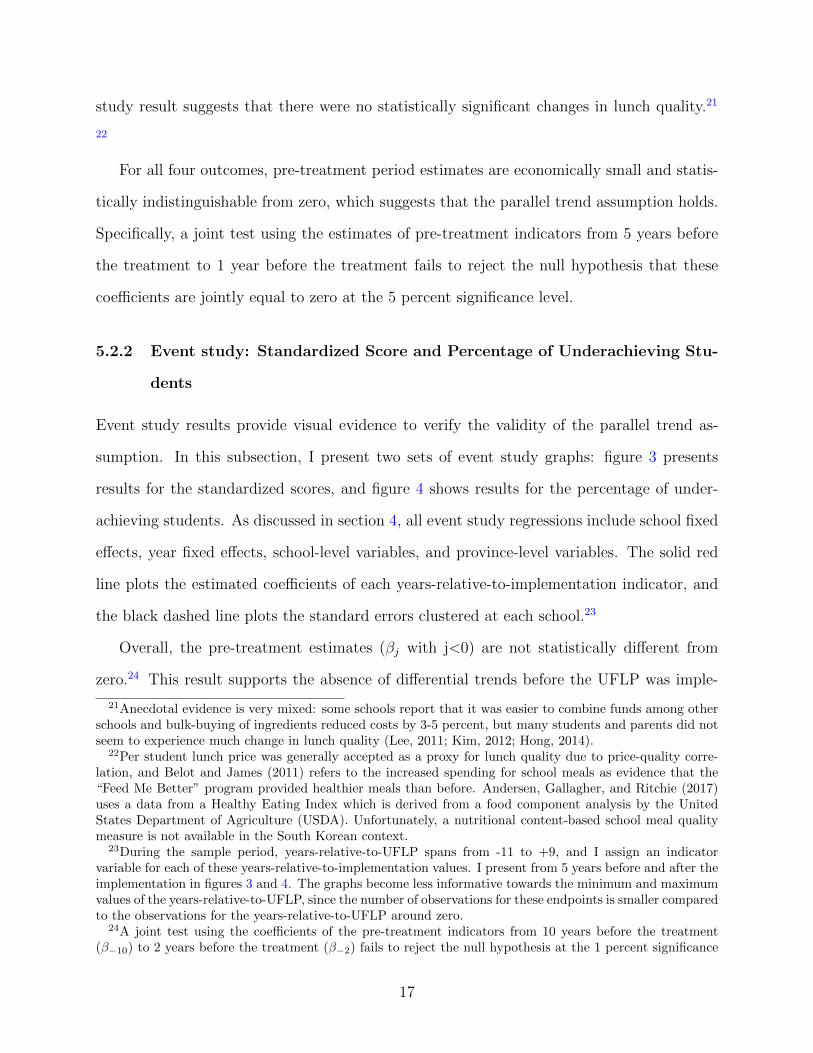
For all four outcomes, pre-treatment period estimates are economically small and statis-

tically indistinguishable from zero, which suggests that the parallel trend assumption holds.

Specifically, a joint test using the estimates of pre-treatment indicators from 5 years before

the treatment to 1 year before the treatment fails to reject the null hypothesis that these

coefficients are jointly equal to zero at the 5 percent significance level.

5.2.2 Event study: Standardized Score and Percentage of Underachieving Stu-

dents

Event study results provide visual evidence to verify the validity of the parallel trend as-

sumption. In this subsection, I present two sets of event study graphs: figure 3 presents

results for the standardized scores, and figure 4 shows results for the percentage of under-

achieving students. As discussed in section 4, all event study regressions include school fixed

effects, year fixed effects, school-level variables, and province-level variables. The solid red

line plots the estimated coefficients of each years-relative-to-implementation indicator, and

the black dashed line plots the standard errors clustered at each school.23

Overall, the pre-treatment estimates (βj with j<0) are not statistically different from

zero.24 This result supports the absence of differential trends before the UFLP was imple-

21Anecdotal evidence is very mixed: some schools report that it was easier to combine funds among otherschools and bulk-buying of ingredients reduced costs by 3-5 percent, but many students and parents did notseem to experience much change in lunch quality (Lee, 2011; Kim, 2012; Hong, 2014).

22Per student lunch price was generally accepted as a proxy for lunch quality due to price-quality corre-lation, and Belot and James (2011) refers to the increased spending for school meals as evidence that the“Feed Me Better” program provided healthier meals than before. Andersen, Gallagher, and Ritchie (2017)uses a data from a Healthy Eating Index which is derived from a food component analysis by the UnitedStates Department of Agriculture (USDA). Unfortunately, a nutritional content-based school meal qualitymeasure is not available in the South Korean context.

23During the sample period, years-relative-to-UFLP spans from -11 to +9, and I assign an indicatorvariable for each of these years-relative-to-implementation values. I present from 5 years before and after theimplementation in figures 3 and 4. The graphs become less informative towards the minimum and maximumvalues of the years-relative-to-UFLP, since the number of observations for these endpoints is smaller comparedto the observations for the years-relative-to-UFLP around zero.

24A joint test using the coefficients of the pre-treatment indicators from 10 years before the treatment(β−10) to 2 years before the treatment (β−2) fails to reject the null hypothesis at the 1 percent significance

17

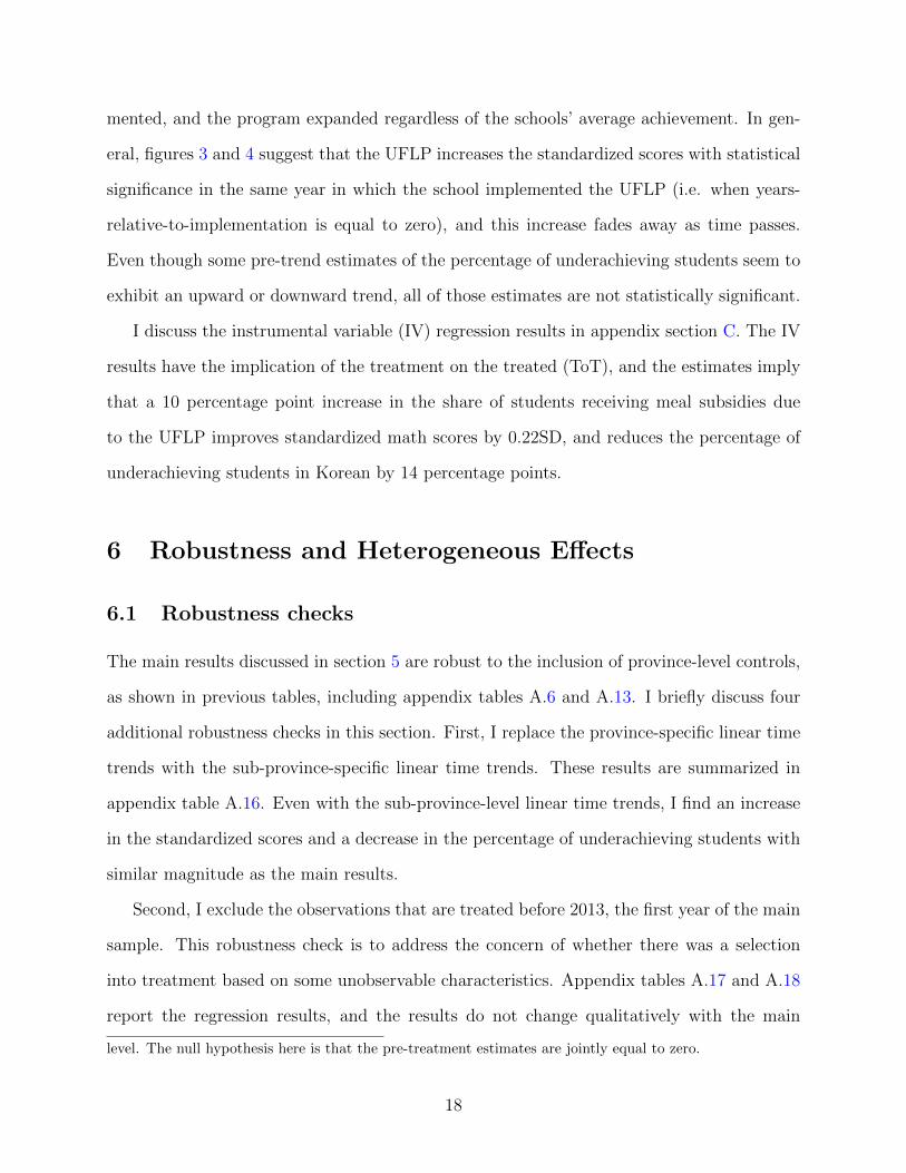
mented, and the program expanded regardless of the schools’ average achievement. In gen-

eral, figures 3 and 4 suggest that the UFLP increases the standardized scores with statistical

significance in the same year in which the school implemented the UFLP (i.e. when years-

relative-to-implementation is equal to zero), and this increase fades away as time passes.

Even though some pre-trend estimates of the percentage of underachieving students seem to

exhibit an upward or downward trend, all of those estimates are not statistically significant.

I discuss the instrumental variable (IV) regression results in appendix section C. The IV

results have the implication of the treatment on the treated (ToT), and the estimates imply

that a 10 percentage point increase in the share of students receiving meal subsidies due

to the UFLP improves standardized math scores by 0.22SD, and reduces the percentage of

underachieving students in Korean by 14 percentage points.

6 Robustness and Heterogeneous Effects

6.1 Robustness checks

The main results discussed in section 5 are robust to the inclusion of province-level controls,

as shown in previous tables, including appendix tables A.6 and A.13. I briefly discuss four

additional robustness checks in this section. First, I replace the province-specific linear time

trends with the sub-province-specific linear time trends. These results are summarized in

appendix table A.16. Even with the sub-province-level linear time trends, I find an increase

in the standardized scores and a decrease in the percentage of underachieving students with

similar magnitude as the main results.

Second, I exclude the observations that are treated before 2013, the first year of the main

sample. This robustness check is to address the concern of whether there was a selection

into treatment based on some unobservable characteristics. Appendix tables A.17 and A.18

report the regression results, and the results do not change qualitatively with the main

level. The null hypothesis here is that the pre-treatment estimates are jointly equal to zero.

18

results.25

Third, I use the total number of students in each school and each year as weights. Ap-

pendix tables A.24 and A.25 present the weighted regression results. In general, the estimates

are comparable to the main results reported in section 5.

Fourth, to examine the possiblity that the results are driven by one province only, I

run 16 regressions by excluding the observations in one province from each. As appendix

figure A.3 shows, the improvements in academic achievement outcomes are not driven by

one province.

Finally, I incorporate recently developed difference-in-differences regression to consider

the potential bias to the average treatment effects on the treated. This will be discussed in

the following subsection.

6.1.1 Results by School Levels

I run the same difference-in-difference regression as in the previous subsections with the

subsample of middle schools and high schools separately in order to investigate the source of

the treatment effects. The middle school subsample spans from 2013 to 2016, and the high

school subsample spans from 2009 to 2016. Among the 9,828 school-by-year observations of

the middle school subsample, 7,568 observations are at least partially treated (77 percent of

the subsample), and 7,147 observations are fully treated. Among the 10,482 school-by-year

observations of the high school subsample, only 850 observations are at least partially treated

(8 percent of the subsample), and 832 observations are fully treated.

For the standardized score outcomes, table A.8 reports the coefficient of interest for

the middle school subsample, and table A.9 presents the coefficient of interest for the high

school subsample. In general, the impacts of the UFLP on the percentage of underachieving

25The mean of standardized scores increased by 0.05, and the sample standard deviations decreased by0.05 by excluding the early-treated observations. It is mechanical to see either a slight increase or decrease inthe sample mean or sample standard deviation since approximately a third of the observations are dropped.Furthermore, standardizing the scores after the exclusion of the early treated schools provided qualitativelythe same results. The results are reported in appendix table A.19.

19

students span from 0.06 SD to 0.12 SD for the high school subsample. The benefits of the

UFLP among the middle school subsample prevails with statistical significance only for the

Korean scores. For math and English scores, the effects were close to zero and statistically

insignificant. In some specifications, small negative coefficients were found.

The reductions in the percentage of underachieving students are mostly found among

the high school subsample. Appendix tables A.10 and A.11 report the regression results

for middle school and high school subsamples, respectively. Even though the point esti-

mates generally suggest that middle schools experienced a reduction in the percentage of

underachieving students, only some of the estimates for Korean and English have statistical

significance. But high schools show a greater reduction across all specifications and academic

subjects.

These differences can be due to data availability: the middle school data is only available

from 2013 to 2016. Considering that more than half of the middle schools were already

treated, and the event study results in section 5.2.2 showing that the beneficial impacts

of the UFLP are concentrated mainly in the early periods after the implementation, not

finding extensive improvements in the standardized scores among middle school students is

not surprising. On the contrary, high schools started to get treated across the provinces

relatively later in the sample period, thus exhibiting the initial positive impact of the UFLP.

Effect on Dropout Rates. For the high school subsample, I utilize dropout information

in the EDSS data and empirically test whether the UFLP caused a reduction in dropout

per 100 students. Since middle school education has been compulsory in the whole country

since 2002, I focus on the high school subsample. Panel A of Table A.12 summarizes the

estimated impact of the UFLP on the number of dropouts per 100 students. No estimates are

statistically significant at any of the conventional significance levels, but the point estimates

imply a 7 percent decrease in dropout rates. Using the standard errors to create bounds, the

estimate is consistent with an 18 percent reduction and a 6 percent increase in the number

20

of dropouts per 100 students.26 In sum, there is not enough evidence to conclude that the

UFLP reduces dropout rates among high school students.

6.1.2 Results for an Alternative Measure of the Percentage of Underachieving

Students

In this subsection, I use an alternative outcome that measures the percentage of under-

achieving students in each school. I examine the effects of the UFLP on the percentage

of the students at the lowest achievement level (“below-basic” level) instead of the sum of

the two lower achievement levels (“below-basic” and “basic” level), which I focused on in

section 5. Focusing on the students at the lowest achievement level also helps understand

who benefits from the UFLP the most across the score distribution.

Panel A of table 4 shows that the UFLP decreases the percentage of students at the lowest

achievement level by approximately 1 to 2 percentage points, or by 21 to 34 percent of the

mean. This benefit appears in both the middle school and high school subsamples. Panel B of

table 4 shows that the middle schools benefit from the reduction in the number of students

who are lowest achieving in Korean and math with statistical significance. Even though

the effects are not statistically significant at conventional levels for English, the estimated

coefficients suggest that the UFLP reduced the percentage of students at the “below-basic”

level by 10 percent of the mean. Panel C of table 4 shows that the UFLP reduced the

percentage of the lowest achieving students by 25 percent to 38 percent of the mean for the

high school subsample. These estimates for the high school subsample were all statistically

significant at the 1 percent level, showing a clear benefit on students’ academic achievement

due to the UFLP. Appendix tables A.13, A.14, and A.15 report the results for sparser or

more saturated models, which lead to qualitatively the same conclusion.

26These bounds are derived by converting each of the bounds of the confidence interval to a percentageusing the mean of the outcome.

21

6.1.3 Results with an Alternative Estimator

In this subsection, I incorporate two of the recently developed methods in the difference-in-

differences literature. Recently, a strand of literature including Borusyak and Jaravel (2017),

de Chaisemartin and D’Haultfoeuille (2020), Callaway and Sant’Anna (2020), Goodman-

Bacon (2020), Sun and Abraham (2020), Athey and Imbens (2021), and Wooldridge (2021)

has demonstrated how the coefficient estimated with the two-way fixed effects linear regres-

sion model is a biased estimate of the average treatment effect (ATE). This bias attached

to the parameter of interest (ATE) can be large if the treatment is heterogeneous over time

within units, and when the treatment has a staggered rollout.

I utilize the new estimator (DIDM) proposed by de Chaisemartin and D'Haultfoeuille

(2020), which can be interpreted as a bias-corrected estimator of the classical difference-in-

differences linear regression model (equation 1). Specifically, the coefficient estimated by

the two-way fixed effects linear regression model can be decomposed into a weighted sum

of average treatment effects of all possible comparisons of each treated group against other

groups (never treated, already-treated, and later-treated), and these possible comparisons

are referred to as 2-by-2 average treatment effects. In extreme cases where these weights

are large negative numbers, even if the individual 2-by-2 average treatment effects are all

positive, the weighted sum can be negative. The DIDM estimator of de Chaisemartin and

D'Haultfoeuille (2020) is particularly suitable for the UFLP’s setting since it allows for the

continuous treatment.27 They also provide another estimator (DIDplM) which plays a similar

role as the pre-treatment coefficient in the classical event study (equation 3).

First, I report the DIDM estimate and show that the estimates reported in section 5 are

robust to this bias correction. Second, I plot the weights of the 2-by-2 estimators to show

that only a few of them are small negative numbers in the case of the UFLP. Third, I present

the DIDplM estimator to ensure that the common trend assumption holds. The common trend

27More detailed discussion regarding de Chaisemartin and D'Haultfoeuille (2020) can be found in appendixsection G.

22

assumption allows the DIDM estimator to have an interpretation of the average treatment

effect.

Table A.26 reports the DIDM estimators, which are similar to the coefficients found in

table 3.28 In general, the DIDM estimates are slightly larger than the ones reported in table

3, implying that the sign of bias is negative. Appendix figure A.4 shows that the very few

weights are negative, and the magnitudes of the negative weights for Korean standardized

scores.29 Table A.26 also reports the placebo estimates (DIDpl,1M and DIDpl,2

M ). These

estimates act as a falsification test and determine whether there were differential trends one

year before the treatment (DIDpl,1M ) or two years before the year of treatment (DIDpl,2

M ).

Finding that the placebo estimates are not significantly different from zero supports the

common trend assumption, which allows DIDM estimates to have an interpretation of the

average treatment effect.

6.2 Heterogeneous Effects by Baseline Participation

In this subsection, I use the information regarding the share of students receiving meal subsi-

dies (Sharesdt) before the UFLP implementation and investigate the possible heterogeneous

effects by a school’s baseline participation in the pre-existing means-tested lunch subsidies.

The UFLP directly affects the share of students on meal subsidy, so it is not a suitable proxy

for the baseline participation after a school implements the UFLP.

Among the observations that are treated after the first year of the sample30, I calculate

the mean of the share within the pre-treated periods. If a school is already treated before the

first year of the sample, there is no available information to calculate the pre-treated period

share.31 I define the schools as having higher baseline participation if the schools have

the average share of participation to the means-tested lunch subsidies greater than equal

28I include the same types of controls as in table 3 for comparison.29Using other academic achievement outcomes does not change the general implication.30The first year would be 2013 for middle schools, and 2009 for high schools.31For the schools that have pre-treated period information, the estimated effects of the UFLP on academic

achievements are qualitatively the same with the full sample results.

23

to the 67th percentile of the distribution of mean of the shares as having higher baseline

participation. I define the schools as having lower baseline participation if the average

share is lower than the 33rd percentile, and rest of the schools as having middle baseline

participation. Using these definitions provides a way to investigate the heterogeneity of the

UFLP’s impacts across baseline participation, while there are no official poverty estimates

for small geographic units.32

I run the same difference-in-differences regression for each of these three subsamples of

schools. Figure 5 summarizes the estimates and standard errors by a school’s baseline par-

ticipation. The exact estimates can be found in column (3) of Appendix tables A.27 through

A.29 for the standaridzed score outcomes, and tables A.30 to A.32 for the percentage of

underachieving students. To summarize, I find general improvement in both of the academic

achievement outcomes in all subsamples. I also use triple-differences regression, which fully

interacts the difference-in-differences model with an indicator for each subsample of schools.

Appendix tables A.33 to A.35 show that the magnitude of reduction in the percentage of

underachieving students in each subsample is not statistically significantly different from

zero.33 34 Previous studies also found similar patterns when the universal meal provision re-

placed the means-tested school meal subsidy. Notably, Ruffini (2020) also finds that students’

math performance improves in districts with low baseline free meal eligibility. Schwartz and

Rothbart (2020) also finds that the Universal Free Meals program in New York City middle

schools improved the test scores of both poor and non-poor students.

Depending on the eligibility for and participation in the means-tested subsidy before the

UFLP, potential benefits are different. First, students with household income low enough

to qualify for and who participated in the means-tested lunch subsidy will benefit from

reduced stigma but there will be no change in incomes. Stigma is a well-known factor

32Only the national yearly series of relative poverty rates are available at KOSIS (Korean StatisticalInformation Service).

33The regression results using the same triple-differences model for the standardized score outcomes alsolead to the same conclusion.

34These results are robust to using either the median or the 25th and 75th percentiles to define higher andlower baseline participation (appendix tables A.36 and A.37)

24

that hinders the take-up of means-tested school meal subsidies (Glantz and Long 1994;

Mirtcheva and Powell 2009; Sandman 2016; Yu, Lim, and Kelly 2019). Second, students

who were eligible for but did not participate in the means-tested subsidy would experience

reduced stigma with increased incomes by saving lunch fees. Third, students who were not

eligible for the means-tested subsidy will benefit from increased income by saving lunch fees.

On average, less than 30 percent of students participated in the means-tested school meal

subsidies before the UFLP, which leaves roughly 70 percent of students’ families experiencing

increased disposable incomes. These benefits differ by household level, but the school-level

data (EDSS) does not have information that I can use to calculate how many students are

from each of the three types of households. In addition, the magnitude of the benefit can

also differ by household income, which is also not detectable.

7 Underlying Mechanisms

In this section, I discuss various potential mechanisms that can contribute to the UFLP’s

positive impact on students’ academic achievement. In subsections 7.1 and 7.2, I provide

suggestive evidence that the UFLP increased educational expenditures.

Previous literature suggests that students react to the expanded access to school meals

in two main ways. First, students participate more in school lunches programs, leading to

better nutrition and cognitive ability (Figlio and Winicki 2005; Hinrichs, 2010; Bartfeld and

Ahn 2011; Frisvold, 2015). This mechanism is particularly effective if the school lunches are

better alternatives (Belot and James 2011; Anderson, Gallagher, and Ritchie 2017; Schwartz

and Rothbardt 2020). Second, students attend school more often, as expanded access to

school lunches can create an additional incentive for students to come to school (Leos-Urbel

et al. 2013; Jayaraman Simroth 2015; Ruffini 2020).

I find that these two previously emphasized mechanisms are unlikely to operate in South

Korea. First, I show with the EDSS data in panel (a) of figure 1 that the share of students

25

who receive lunch from their schools has been stable and close to one both before and after

the UFLP implementation. This suggests that it is not likely that the UFLP increased

participation in school lunch programs in South Korea.35 In addition, I find that the per-

student school meal expenditure, which can be a proxy for meal quality, did not change

significantly (table 2 and figure 2).36 Second, South Korea is one of the countries that do not

face a severe truancy problem (OECD 2019), implying that the margin for an improvement

in attendance is small. I support this argument by showing that there is no change in the

proportion of students who have taken the national standardized test (table A.39). Since

there is no attendance information in the EDSS data, this is indirect evidence that the UFLP

did not seem to change attendance.37

Notably, the UFLP might reduce stigma by decreasing family income salience since it

does not require means-testing. The findings of Gennetian et al. (2004) and Clark-Kaufman,

Duncan, and Morris (2003) suggest that the reduced stigma could improve students’ aca-

demic performance. However, EDSS data is not fit for the task of investigating the change

in stigma due to the implementation of the UFLP.

7.1 After-School Program Participation Change using EduData

Service System (EDSS) data

In this subsection, I focus on the effect of the UFLP on after-school program participation

using the information in the EDSS data. As discussed in section 2, the UFLP increased

disposable income for students’ families by saving lunch fees. In addition to the income

effect, mental accounting framework (Thaler 1990, 1998, and 1999) suggests an increase in

35The first quartile of the share of students who received lunches from their school is 0.98.36If schools increased the caloric content or the glucose level to boost the students’ cognitive function on

the test day or the few days around it as found in Figlio and Winicky (2005), this change is unlikely to becaptured in the yearly frequency of the EDSS data.

37Table A.39 also addresses the concern that schools at risk of accountability sanctions will manipulatethe testing pool (Figlio and Winicki 2005). Specifically, studies have documented that schools intentionallymisclassify the low-performing students as disabled or absent on the day of the test (Cullen and Reback2002; Figlio and Getzler, 2002; Jacob, 2002).

26

expenditures in educational investment. Since the parents would have paid the after-school

program fees using the same designated banking account for the lunch fees before the UFLP,

this institutional detail also could contribute to mental accounting.

I use the same difference-in-differences framework in section 4 and find that average after-

school program participation increased by 0.03 programs on average, as shown in table 5. I

focus on the average number of after-school programs in which the students participate in

each school, which is obtained by dividing the total number of programs offered by the total

number of participants. The EDSS data has information on academic and non-academic

programs separately, and the regression results suggest that the academic after-school pro-

gram participation is the source of increased overall participation in after-school programs.38

Typical academic after-school programs include math, English, and writing, which can help

the students with exam scores and course materials. The estimated effect corresponds to a

16 percent increase in average participation in the after-school programs, and a 22 percent

increase in average academic after-school program participation. This result is directly com-

parable to Hener (2017)’s findings that child benefit expansion in Germany increased educa-

tion expenditures by 18 percent, and child-assignable expenditures by 37 percent. Notably,

average participation in non-academic after-school programs does not show a statistically

significant change due to the UFLP.

The back-of-the-envelope calculation suggests that the parents spend approximately 20

percent of the saved lunch expenses on academic after-school program participation. These

programs are generally not free, and the average fee to participate in an after-school program

on average is 20 USD to 30 USD per month, which has been stable over time (National

Assembly Budget Office 2009; Lee and Hwang 2016; OECD 2012). Using the estimated

increase in academic after-school program participation (0.4 more programs) and assuming

this increase remained through the whole year, the back-of-the-envelope calculation gives

a 144 USD increase in after-school program expenses per year (12 months × 0.4 programs

38Increased academic after-school program participation is robust to sparser or more saturated models(table A.40).

27

× 30 dollars = 144 dollars). Comparing this amount to the saved lunch expense for the

parents implies that the parents are spending approximately 20 percent of the saved expense

on academic after-school program participation.

7.2 Household after-school Program Expenditure Change using

the Private Education Expenditure Survey

This subsection uses another data source to supplement the findings in section 7.1, to corrob-

orate the increased after-school program participation. Using Private Education Expendi-

tures Survey (PES) data, I estimate the impacts of the UFLP rollout on after-school program

participation and expenditures.

I use a regression model similar to the difference-in-differences model described in section

4, but there are adjustments due to the different data structure. PES data is student-level

repeated cross-section data and does not have detailed enough geographic information to

define the treatment intensity as the share of students affected by the UFLP in each school.

Instead, I define the treatment intensity using the share of schools in each year for every

province using the EDSS data. Since the geographical information in the PES data has less

detail, the treatment definition of the PES data is bound to have a larger measurement error

than that of the EDSS data. Table A.43 reports the summary statistics for the PES data.

For the PES data, I use the following regression equation:

Yihdt = βUFLPsharePESdt + ΦXPES

iht + µd + µd × t+ µt + eihdt, (4)

where Yihdt is the after-school program participation or expenditure of student i in household

h in province d in year t. DPESdt ranges from 0 to 1 and represents the probability that students

in province d in year t are in a school with universal free lunch provision due to the UFLP.

Unlike the case of the school-level regression using the EDSS data, the value of DPESdt does

not differ in the same province. To accentuate the different definition of the treatment and

28

the additional controls in the regression model for the Private Education Expenditure Survey

compared to the regression in section 4, I use superscript PES notation on the treatment

(DPESdt ) and the controls (XPES

iht ). I consider both the log and the inverse hyperbolic sine

transformation of the after-school programs’ expenditure since there are outliers.39

XPESiht stands for student-level controls such as students’ gender, school-level indicator

(middle or high school) and students’ previous achievement categories (the top 10 percent,

11 to 30 percent, 31 to 60 percent, 61 to 80 percent, the lowest 20 percent in class, reported

by the homeroom teacher of each student). µd represents geographic fixed effects including

province and urban fixed effects, and µt represents the year fixed effects. To closely follow

the preferred specification, I also include the province-specific linear time trends, denoted by

µd × t. The standard errors are clustered at each province by each school level by urban or

rural indicator by year (17×2×2×8=544 clusters).

The results from the PES data suggest a statistically significant and economically mean-

ingful increase in participation, which corroborates the findings from the EDSS data. Column

(1) of table A.44 reports that the participation rate increased by 10 percentage points, which

implies a 14 percent increase with high statistical significance.40 Moreover, the results in

columns (2) and (3) of table A.44 suggest that the average expenditures on the after-school

programs also increased. The coefficients reported in columns (2) and (3) show the treat-

ment effect on the growth rate of the expenditures on after-school programs. The estimated

effects of the implementation of the UFLP suggest an approximately 20 percent increase in

expenditures on after-school programs, which can be translated into a 4.5 USD increase per

month on average. Putting this result into yearly expenditures implies an approximately 53

(=4.5 × 12) USD increase in expenditures on after-school programs.

This increased expense consists of 8 to 10 percent of the increased disposable income

39The inverse hyperbolic sine transformation approximates the log transformation but accommodates zerossince the domain of the inverse hyperbolic sine function contains zero.

40The mean participation rate is 70 percent throughout the sample. Among the observations with treat-ment equal to zero (which means that no school in the province in that year is treated), 73 percent of studentsparticipate in the after-school programs.

29

by saving the lunch fees due to the UFLP, which supports the back-of-the-envelope calcu-

lation using the increased participation in the after-school programs from the EDSS data.

Specifically, the back-of-the-envelope calculation of the increase in the after-school program

expenditures found in the EDSS data is greater than the increase found from utilizing the

PES data. But the after-school program participation and expenditure information in the

PES data combines both academic and non-academic programs, unlike the EDSS. Moreover,

the PES is a survey and the EDSS is administrative data, not to mention the different data

structure. Given these innate differences between the two data sets, it is unlikely that the

estimates will be the same.

Using the family income information in the PES data, figure A.5 plots the coefficients and

the standard errors for different income groups separately (monthly income 3,000 USD or

below, between 3,000 and 6,000, and 6,000 or above). Note that the eligibility threshold for

the means-tested school lunch subsidies is approximately 2,500 USD: thus the majority of the

first income group is eligible.41 According to panel (a) of figure A.5, all three subsamples show

a statistically significant increase in after-school program participation. Panel (b) shows that

the expenditures on the after-school programs also increased statistically significantly for the

families with monthly incomes of 3,000 USD or below. Middle and higher income groups do

not show statistically significant increases in log of expenditures, but the level values show

similar magnitude of increases. Transforming the log increase in panel B of figure A. 5 into the

level amount, the estimates suggest that the expenditures increased by 13 USD (7 percent)

for the lower income group, and approximately by 11 USD (5 percent) for the middle and

higher income groups. To summarize, the results from the PES data also suggest that the

households respond to the UFLP by increasing the after-school program participation, even

though the increase in expenditures on the after-school program participation varies across

41For families with three members, the eligibility threshold is approximately $2,050, and for families withfour members, the eligibility threshold is approximately $2,500. Average family size during the sample periodis approximately 2.7 (Statistics Korea 2021) Still, there can be misreporting of income groups since this issurvey data.

30

different income groups.42 Still, there is a possibility that the UFLP improves students’

academic achievement through a channel that is not discussed in this paper, and parents

increase the education investment as a response to the higher return on the investment.

8 Conclusion

This paper examines the Universal Free Lunch Program’s effect on students’ academic

achievement in South Korea. By utilizing administrative school-level data and the program

rollout information, I implement difference-in-differences and IV frameworks to estimate the

Universal Free Lunch Program’s causal effect. I find strong evidence of a reduction in the

percentage of underachieving students, and an increase in standardized scores, which was

comparable to the effects found in other contexts.

I find that the UFLP’s beneficial impact prevails universally in schools with different in-

come levels. I provide empirical and anecdotal evidence that the UFLP acted as an in-kind

transfer to relatively higher income families. By examining numerous potential underlying

mechanisms, I show that the South Korean context does not harm the generalizability of

the results, but provides a setting where a new mechanism can be highlighted. This paper

provides suggestive evidence of an underlying mechanism that highlights parents’ educa-

tional investment. Even though the higher income families are less income constrained, the

mental accounting of parents can lead to an economically meaningful increase in educational

investment. It is likely that the saved lunch fees are perceived as an increased budget for

educational expenditures but not for other categories of consumption.

There are government budgetary concerns regarding the universal provision of school

meals, as it does not target the neediest population and thus uses the resource inefficiently.

One approach to analyze the efficiency is to derive the cost-effectiveness of the UFLP. I follow

Dhaliwal et al. (2013) to claculate the cost-effectiveness of the UFLP using the estimates

42I find neither economically meaningful nor statistically significant results for the intensive margin (byusing only the observations with nonzero expenditures on after-school programs). I also do not find anydistinct pattern across income groups by investigating the intensive margin of after-school program spending.

31

provided in section 5.43 The effectiveness-cost ratio estimate suggests that per-student annual

expenditures on the UFLP increases standardized test scores by 0.07SD for Korean, 0.05SD

for math, and 0.04 SD for English. These magnitudes are comparable to several programs in

the US setting (Yeh 2010), including Summer school, a 10 percent increase in spending, and

class size reduction (Nye et al. 2001; Finn et al. 2001). This leads to the conclusion that

the UFLP is relatively cost-effective even though it does not explicitly aim to raise student

achievement.44

The empirical evidence the UFLP’s impacts in South Korea sheds light on the program’s

impact in other countries with similar contexts, such as high stigma and high take-up of pre-

existing means-tested school meal subsidies. As many countries have means-tested school

meal subsidies as part of their redistribution measures, the benefit of the UFLP provides ev-

idence that seemingly misaligned in-kind transfers can nudge parents’ consumption towards

children’s educational investment.

43I provide detailed explanation on the implementation of Dhaliwal et al. (2013) in appendix section F.44However, including the measurement error issues regarding the cost, the cost-effectiveness of the UFLP

can have limited generalizability. For example, if other countries were to adopt the program, depending onthe institutional context, the cost to implement this program can be much higher than the cost in SouthKorea. Since the early 1990s, almost 100 percent of students in South Korea have received lunch through theirschools, and thus the essential equipment and staffs to provide lunch to all students were already in place.If this is not the case in other settings, the program’s cost increases and thus reduces the cost-effectivenessof the program.

32

References

Lee, David L., et al. “Valid t-ratio Inference for IV.” arXiv preprint arXiv:2010.05058 (2020).Abraham, Sarah, and Liyang Sun. “Estimating dynamic treatment effects in event studies

with heterogeneous treatment effects.” arXiv preprint arXiv:1804.05785 (2018).Finkelstein, Amy, and Matthew J. Notowidigdo. “Take-up and targeting: Experimental

evidence from SNAP.” The Quarterly Journal of Economics 134.3 (2019): 1505-1556.Bhargava, Saurabh, and Dayanand Manoli. “Psychological frictions and the incomplete take-

up of social benefits: Evidence from an IRS field experiment.” American EconomicReview 105.11 (2015): 3489-3529.

Gordon, Nora E., and Krista J. Ruffini. School nutrition and student discipline: Effects ofschoolwide free meals. No. w24986. National Bureau of Economic Research, 2018.

Frisvold, David E. “Nutrition and cognitive achievement: An evaluation of the School Break-fast Program.” Journal of public economics 124 (2015): 91-104.

Chakraborty, Tanika, and Rajshri Jayaraman. “School feeding and learning achievement:Evidence from India’s midday meal program.” Journal of Development Economics139 (2019): 249-265.

Hinrichs, Peter. “The effects of the National School Lunch Program on education andhealth.” Journal of Policy Analysis and Management 29.3 (2010): 479-505.

Anderson, Michael L., Justin Gallagher, and Elizabeth Ramirez Ritchie. School lunch qualityand academic performance. No. w23218. National Bureau of Economic Research,2017.

Bhattacharya, Jayanta, Janet Currie, and Steven J. Haider. “Breakfast of champions? TheSchool Breakfast Program and the nutrition of children and families.” Journal ofHuman Resources 41.3 (2006): 445-466.

Chakraborty, Tanika, and Rajshri Jayaraman. “School feeding and learning achievement:Evidence from India’s midday meal program.” Journal of Development Economics139 (2019): 249-265.

Gordon, Nora, and Krista Ruffini. “Schoolwide Free Meals and Student Discipline: Effectsof the Community Eligibility Provision.” Education Finance and Policy (2019): 1-50.

Ruffini, Krista. “Universal access to free school meals and student achievement: Evidencefrom the Community Eligibility Provision.” (2020). Journal of Human Resources,Forthcoming.

Arulampalam, Wiji, Robin A. Naylor, and Jeremy Smith. “Am I missing something? Theeffects of absence from class on student performance.” Economics of Education review31.4 (2012): 363-375.

Lamarche, Carlos. “Private school vouchers and student achievement: A fixed effects quan-tile regression evaluation.” Labour Economics 15.4 (2008): 575-590.

Tavares, Priscilla Albuquerque. “The impact of school management practices on educationalperformance: Evidence from public schools in Sao Paulo.” Economics of EducationReview 48 (2015): 1-15.

Machado, Jose AF, and JMC Santos Silva. “Quantiles via moments.” Journal of Economet-rics 213.1 (2019): 145-173.

33

MacKinnon, James G. “How clusterarobust inference is changing applied econometrics.”Canadian Journal of Economics/Revue canadienne d’economique 52.3 (2019): 851-881.

Carrell, Scott E., and Mark L. Hoekstra. “Externalities in the classroom: How childrenexposed to domestic violence affect everyone’s kids.” American Economic Journal:Applied Economics 2.1 (2010): 211-28.

Carrell, Scott E., Mark Hoekstra, and Elira Kuka. “The long-run effects of disruptive peers.”American Economic Review 108.11 (2018): 3377-3415.

Altindag, Duha T., et al. “Free lunch for all? The impact of universal school lunch onstudent misbehavior.” Economics of Education Review 74 (2020): 101945.

Baek, Deokrye, Yongjun Choi, and Hong Lee. “Universal welfare may be costly: Evidencefrom school meal programs and student fitness in South Korea.” Sustainability 11.5(2019): 1290.

Santana, C. C. A., et al. “Physical fitness and academic performance in youth: A systematicreview.” Scandinavian Journal of Medicine & Science in Sports 27.6 (2017): 579-603.

Borusyak, Kirill, and Xavier Jaravel. “Revisiting event study designs.” Available at SSRN2826228 (2017).

Goodman-Bacon, Andrew. “Difference-in-differences with variation in treatment timing.”No. w25018. National Bureau of Economic Research, 2018.

Callaway, Brantly, and Pedro HC Sant’Anna. “Difference-in-differences with multiple timeperiods and an application on the minimum wage and employment.” arXiv preprintarXiv:1803.09015 (2018).

OECD. “PISA 2018 Results (Volume III): What School Life Means for Students’ Lives.”OECD, 2019.

Belot, Michele, and Jonathan James. “Healthy school meals and educational outcomes.”Journal of health economics 30.3 (2011): 489-504.

Schwartz, Amy Ellen, and Michah W. Rothbart. “Let them eat lunch: The impact of univer-sal free meals on student performance.” Journal of Policy Analysis and Management39.2 (2020): 376-410.

Anderson, Michael L., Justin Gallagher, and Elizabeth Ramirez Ritchie. “School meal qual-ity and academic performance.” Journal of Public Economics 168 (2018): 81-93.

Gordanier, John, et al. “Free lunch for all! the effect of the community eligibility provisionon academic outcomes.” Economics of Education Review 77 (2020): 101999.

Bartfeld, Judith S., and Hong-Min Ahn. “The School Breakfast Program strengthens house-hold food security among low-income households with elementary school children.”The Journal of nutrition 141.3 (2011): 470-475.

Evans, Landon W. “The Effect of Free and Reduced Lunch on Reading and Math Achieve-ment.” (2015).

OECD. “OECD Reviews of School Resources.” (2017). (click here for the link)Ashenfelter, Orley, and Cecilia Rouse. “Income, schooling, and ability: Evidence from a

new sample of identical twins.” The Quarterly Journal of Economics 113.1 (1998):253-284.

Angrist, Joshua D., and Alan B. Keueger. “Does compulsory school attendance affect school-ing and earnings?.” The Quarterly Journal of Economics 106.4 (1991): 979-1014.

34

Hitt, Collin, Michael Q. McShane, and Patrick J. Wolf. “Do impacts on test scores evenmatter? Lessons from long-run outcomes in school choice research: Attainment versusachievement impacts and rethinking how to evaluate school choice programs.” AEIPaper & Studies (2018): 3e.

McEwan, Patrick J. “The impact of Chile’s school feeding program on education outcomes.”Economics of Education Review 32 (2013): 122-139.

Lee, Kyungmi. “Trick to get through the inflation for the Universal Free Lunch Program”Hankyoreh, 21 March 2011, http://www.hani.co.kr/arti/PRINT/466372.html. Ac-cessed 28 January 2021.

Hong, Yongduk. “Bulk-buying power of the school meals” Hankyoreh, 27 March 2014,http://www.hani.co.kr/arti/area/area general/630257.html. Accessed 28 Jan-uary 2021.

Kim, Kyungho. “Schools are expanding bulk-buying of the school meal ingredients” FoodService News, 6 September 2012, (click here for the link). Accessed 28 January 2021.

Ryu, Inha, Bonghyun Kim, Jaeduk Lee, and Jeewon Nam. “My mother is happy that shedoesn’t have to worry about the lunch fees anymore” The Kyunghyang Shinmun, 1November 2011, (click here for the link). Accessed 18 July 2021.

Figlio, David N., and Joshua Winicki. “Food for thought: the effects of school accountabilityplans on school nutrition.” Journal of public Economics 89.2-3 (2005): 381-394.

De Chaisemartin, Clement, and Xavier d’Haultfoeuille. “Two-way fixed effects estima-tors with heterogeneous treatment effects.” American Economic Review 110.9 (2020):2964-96.

Shapiro, Eliza. “Coronavirus in N.Y.C.: Why Closing Public Schools Is a ‘Last Resort’ ”New York Times, 7 March 2020, https://www.nytimes.com/2020/03/07/nyregion/nyc-schools-coronavirus.html. Accessed 30 May 2021.

Akee, Randall KQ, et al. “Parents’ incomes and children’s outcomes: a quasi-experimentusing transfer payments from casino profits.” American Economic Journal: AppliedEconomics 2.1 (2010): 86-115.

Milligan, Kevin, and Mark Stabile. “Do child tax benefits affect the well-being of children?Evidence from Canadian child benefit expansions.” American Economic Journal:Economic Policy 3.3 (2011): 175-205.

Dahl, Gordon B., and Lance Lochner. “The impact of family income on child achievement:Evidence from the earned income tax credit.” American Economic Review 102.5(2012): 1927-56.

Lee, Joonho, and Hyesun Hwang. “Private Educational Expenditure According to Purposesof Private Education and after-school Program Participation.” Journal of KoreanHome Management Association 34.2 (2016): 1-14.

National Assembly Budget Office. “after-school Program Evaluation Report.” (2009).https://nabo.go.kr/s/ODIzNzMw. Accessed 19 April 2021.

Organisation for Economic Coaoperation and Development (OECD). “PISA 2012 results:What makes schools successful? Resources, policies and practices (volume IV).”(2013).

Korea Labor Institute (KLI). “After-school Programs and Promoting the Growth of SocialEnterprises.” (2010). https://www.moe.go.kr/boardCnts/fileDown.do?m=030202&s=moe&fileSeq=8e37f381709d19069e3bb9e91c11866e. Accessed 19 April 2021.

35

Hener, Timo. “Effects of labeled child benefits on family savings.” Review of Economics ofthe Household 15.3 (2017): 759-777.

Jones, Lauren E., Kevin Milligan, and Mark Stabile. “Child cash benefits and family ex-penditures: Evidence from the National Child Benefit.” Canadian Journal of Eco-nomics/Revue canadienne d’economique 52.4 (2019): 1433-1463.

Dhaliwal, Iqbal, et al. “Comparative cost-effectiveness analysis to inform policy in developingcountries: a general framework with applications for education.” Education policy indeveloping countries 17 (2013): 285-338.

Zhuang, Juzhong, et al. “Theory and practice in the choice of social discount rate for cost-benefit analysis: a survey.” No. 94. ERD working paper series, 2007.

Yeh, Stuart S. “The cost effectiveness of 22 approaches for raising student achievement.”Journal of Education Finance (2010): 38-75.

U.S. Bureau of Economic Analysis, Gross Domestic Product: Implicit Price Deflator, re-trieved from FRED, Federal Reserve Bank of St. Louis; (click here for the link),April 10, 2021. [A191RI1A225NBEA]

University of Groningen and University of California, Davis, Exchange Rate (market+estimated)for Republic of Korea [XRNCUSKRA618NRUG], retrieved from FRED, Federal Re-serve Bank of St. Louis; (click here for the link), April 10, 2021.

Pollard, Christina M., and Sue Booth. “Food insecurity and hunger in rich countriesait istime for action against inequality.” International journal of environmental researchand public health 16.10 (2019): 1804.

Statistics Korea (2021), Average family size. (click here for the link) (Accessed on 28 Septem-ber 2021)

OECD (2021a), Enrolment rate in secondary and tertiary education (indicator). (click herefor the link) (Accessed on 16 July 2021) doi: 10.1787/1d7e7216-en

OECD (2021b), Secondary graduation rate (indicator). doi: 10.1787/b858e05b-en (click herefor the link) (Accessed on 16 July 2021)

Finkelstein, Amy. “E-Z Tax: Tax Salience and Tax Rates.” Forthcoming in The QuarterlyJournal of Economics 124 No. 3 (August, 2009).

Saez, Emmanuel. “Do Tax Filers Bunch at Kink Points? Evidence, Elasticity Estimation,and Salience Effects.” University of California at Berkeley. Mimeo, 2009.

Congdon, William J., Jeffrey R. Kling, and Sendhil Mullainathan. “Behavioral economicsand tax policy.” National Tax Journal 62.3 (2009): 375-386.

Hoynes, Hilary W., and Diane Whitmore Schanzenbach. “Safety net investments in chil-dren.” No. w24594. National Bureau of Economic Research, 2018.

Lee, Eun-Hwa, and Se-Jeong Yang. “Wife-Husband Role Division on Household Finan-cial Management: Comparing Between Dual Income Household and Single IncomeHousehold.” Journal of Korean Home Management Association 26.6 (2008): 143-158.

Kenney, Catherine T. “Father doesn’t know best? Parents’ control of money and childrenasfood insecurity.” Journal of Marriage and Family 70.3 (2008): 654-669.

Gordanier, John, et al. “Free lunch for all! the effect of the community eligibility provisionon academic outcomes.” Economics of Education Review 77 (2020): 101999.

Berry, James, et al. “Implementation and effects of India’s national school-based iron sup-plementation program.” Journal of Development Economics 144 (2020): 102428.

36

Gordanier, John, et al. “Free lunch for all! the effect of the community eligibility provisionon academic outcomes.” Economics of Education Review 77 (2020): 101999.

Gundersen, Craig, Brent Kreider, and John Pepper. “The impact of the National SchoolLunch Program on child health: A nonparametric bounds analysis.” Journal of Econo-metrics 166.1 (2012): 79-91.

Handbury, J., and S. Moshary. School Food Policy Affects Everyone: Retail Responses tothe National School Lunch Program. Working paper, 2020.

Kim, Hyanglan. Geochang County Council meeting log. (2015). (click here for the link).Accessed 27 July 2021.

Lee, Youngsik. Gyeongsangbuk-do province Council meeting log. (2018). (click here for thelink). Accessed 27 July 2021.

Lee, Taeson. Daegu Metropolitan Council meeting log. (2020). (click here for the link).Accessed 27 July 2021.

Lee, Namsook. Jeonju City Council meeting log. (2020). (click here for the link). Accessed27 July 2021.

Ryu, Myoungyeol. Gimhae City Council meeting log. (2021). (click here for the link).Accessed 27 July 2021.

Korea Financial Telecommunications & Clearings Institute (KFTC). “School Cash Manage-ment Service.” https://www.cmsedi.or.kr/cms/info/outline/school. Accessed 9August 2021.

Uhm, Taemin. “Gyeonggi Provincial Office of Education implements “school banking sys-tem.” Korea JoongAng Daily, 16 October 1997, https://news.joins.com/article/3535373. Accessed 9 August 2021.

Jeong, Yong-baek. “Busan Metropolitan Office of Education implements “school bank-ing system.” Korea JoongAng Daily, 15 February 1997, https://news.joins.com/article/3402900. Accessed 9 August 2021.

Hyeon, Ha-young., and Dong-joon Shin. “Provincial education finance: tax revenue andexpenditure analysis.” (2016). (click here for the link). Accessed 17 August 2021.

Ministry of Education. “Provincial Education Finance Information.” (2021). https:

//eduinfo.go.kr/portal/theme/housekeepingTap2Page.do. Accessed 17 August2021.

Choe, Sang-Hun. “Seoul Mayor Resigns After Losing School Lunch Referendum” The NewYork Times, 25 August 2011, https://www.nytimes.com/2011/08/27/world/asia/27korea.html. Accessed 17 August 2021.

Choe, Sang-Hun. “In First, South Korea Votes on Social Policy” The New York Times, 24August 2011, https://www.nytimes.com/2011/08/25/world/asia/25korea.html. Ac-cessed 17 August 2021.

Woo, Seokjin, Soohyung Lee, and Kyunghee Kim. “Carrot and stick?: Impact of a low-stakes school accountability program on student achievement.” Economics Letters137 (2015): 195-199.

Gennetian, L. A., Duncan, G., Knox, V., Vargas, W., Clark-Kauffman, E., London, A.S. (2004). “How welfare policies affect adolescentsa school outcomes: A synthesisof evidence from experimental studies.” Journal of Research on Adolescence, 14(4),399-423.

37

Clark-Kauffman, Elizabeth, Greg J. Duncan, and Pamela Morris. “How welfare policiesaffect child and adolescent achievement.” American Economic Review 93.2 (2003):299-303.

38

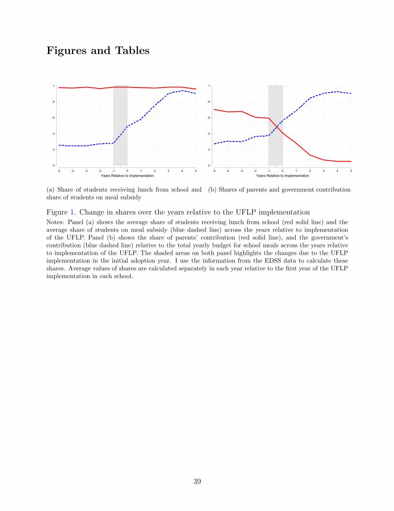
Figures and Tables

0

.2

.4

.6

.8

1

-5 -4 -3 -2 -1 0 1 2 3 4 5

Years Relative to Implementation

(a) Share of students receiving lunch from school andshare of students on meal subsidy

0

.2

.4

.6

.8

1

-5 -4 -3 -2 -1 0 1 2 3 4 5

Years Relative to Implementation

(b) Shares of parents and government contribution

Figure 1. Change in shares over the years relative to the UFLP implementationNotes: Panel (a) shows the average share of students receiving lunch from school (red solid line) and theaverage share of students on meal subsidy (blue dashed line) across the years relative to implementationof the UFLP. Panel (b) shows the share of parents’ contribution (red solid line), and the government’scontribution (blue dashed line) relative to the total yearly budget for school meals across the years relativeto implementation of the UFLP. The shaded areas on both panel highlights the changes due to the UFLPimplementation in the initial adoption year. I use the information from the EDSS data to calculate theseshares. Average values of shares are calculated separately in each year relative to the first year of the UFLPimplementation in each school.

39

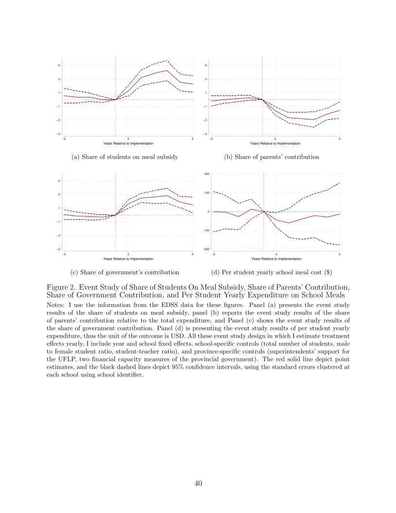
−.5

−.3

−.1

.1

.3

.5

−5 0 5

Years Relative to Implementation

(a) Share of students on meal subsidy

−.5

−.3

−.1

.1

.3

.5

−5 0 5

Years Relative to Implementation

(b) Share of parents’ contribution

−.5

−.3

−.1

.1

.3

.5

−5 0 5

Years Relative to Implementation

(c) Share of government’s contribution

−200

−100

0

100

200

−5 0 5

Years Relative to Implementation

(d) Per student yearly school meal cost ($)

Figure 2. Event Study of Share of Students On Meal Subsidy, Share of Parents’ Contribution,Share of Government Contribution, and Per Student Yearly Expenditure on School MealsNotes: I use the information from the EDSS data for these figures. Panel (a) presents the event studyresults of the share of students on meal subsidy, panel (b) reports the event study results of the shareof parents’ contribution relative to the total expenditure, and Panel (c) shows the event study results ofthe share of government contribution. Panel (d) is presenting the event study results of per student yearlyexpenditure, thus the unit of the outcome is USD. All these event study design in which I estimate treatmenteffects yearly, I include year and school fixed effects, school-specific controls (total number of students, maleto female student ratio, student-teacher ratio), and province-specific controls (superintendents’ support forthe UFLP, two financial capacity measures of the provincial government). The red solid line depict pointestimates, and the black dashed lines depict 95% confidence intervals, using the standard errors clustered ateach school using school identifier.

40

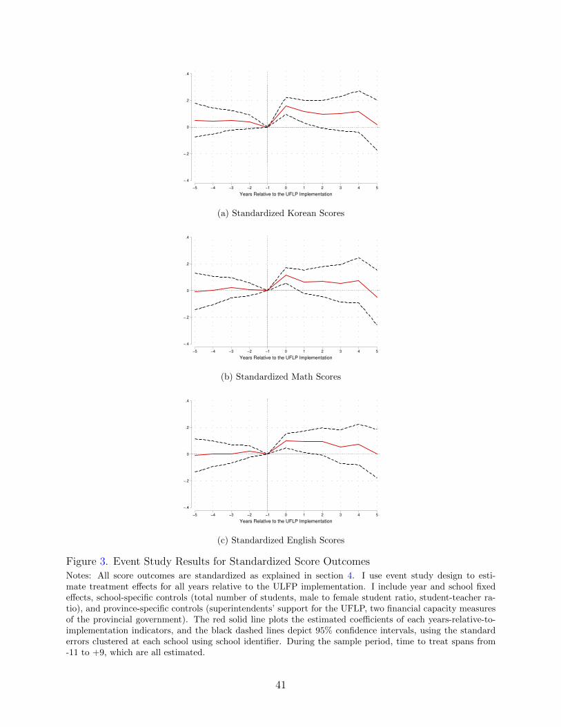
−.4

−.2

0

.2

.4

−5 −4 −3 −2 −1 0 1 2 3 4 5

Years Relative to the UFLP Implementation

(a) Standardized Korean Scores

−.4

−.2

0

.2

.4

−5 −4 −3 −2 −1 0 1 2 3 4 5

Years Relative to the UFLP Implementation

(b) Standardized Math Scores

−.4

−.2

0

.2

.4

−5 −4 −3 −2 −1 0 1 2 3 4 5

Years Relative to the UFLP Implementation

(c) Standardized English Scores

Figure 3. Event Study Results for Standardized Score OutcomesNotes: All score outcomes are standardized as explained in section 4. I use event study design to esti-mate treatment effects for all years relative to the ULFP implementation. I include year and school fixedeffects, school-specific controls (total number of students, male to female student ratio, student-teacher ra-tio), and province-specific controls (superintendents’ support for the UFLP, two financial capacity measuresof the provincial government). The red solid line plots the estimated coefficients of each years-relative-to-implementation indicators, and the black dashed lines depict 95% confidence intervals, using the standarderrors clustered at each school using school identifier. During the sample period, time to treat spans from-11 to +9, which are all estimated.

41

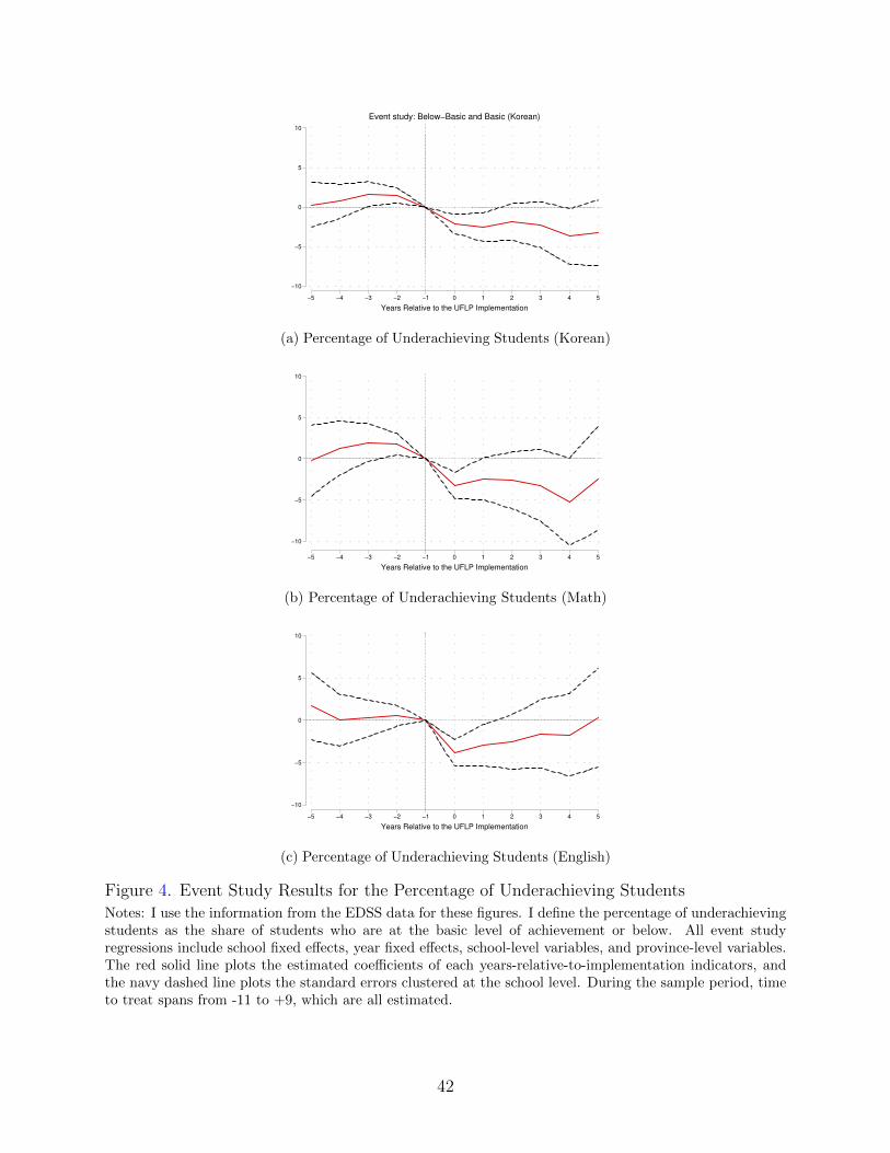
−10

−5

0

5

10

−5 −4 −3 −2 −1 0 1 2 3 4 5

Years Relative to the UFLP Implementation

Event study: Below−Basic and Basic (Korean)

(a) Percentage of Underachieving Students (Korean)

−10

−5

0

5

10

−5 −4 −3 −2 −1 0 1 2 3 4 5

Years Relative to the UFLP Implementation

(b) Percentage of Underachieving Students (Math)

−10

−5

0

5

10

−5 −4 −3 −2 −1 0 1 2 3 4 5

Years Relative to the UFLP Implementation

(c) Percentage of Underachieving Students (English)

Figure 4. Event Study Results for the Percentage of Underachieving StudentsNotes: I use the information from the EDSS data for these figures. I define the percentage of underachievingstudents as the share of students who are at the basic level of achievement or below. All event studyregressions include school fixed effects, year fixed effects, school-level variables, and province-level variables.The red solid line plots the estimated coefficients of each years-relative-to-implementation indicators, andthe navy dashed line plots the standard errors clustered at the school level. During the sample period, timeto treat spans from -11 to +9, which are all estimated.

42

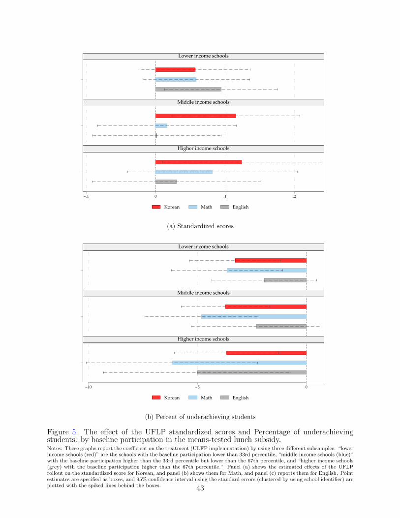
−.1 0 .1 .2

Lower income schools

Middle income schools

Higher income schools

Korean Math English

(a) Standardized scores

−10 −5 0

Lower income schools

Middle income schools

Higher income schools

Korean Math English

(b) Percent of underachieving students

Figure 5. The effect of the UFLP standardized scores and Percentage of underachievingstudents: by baseline participation in the means-tested lunch subsidy.Notes: These graphs report the coefficient on the treatment (ULFP implementation) by using three different subsamples: “lowerincome schools (red)” are the schools with the baseline participation lower than 33rd percentile, “middle income schools (blue)”with the baseline participation higher than the 33rd percentile but lower than the 67th percentile, and “higher income schools(grey) with the baseline participation higher than the 67th percentile.” Panel (a) shows the estimated effects of the UFLProllout on the standardized score for Korean, and panel (b) shows them for Math, and panel (c) reports them for English. Pointestimates are specified as boxes, and 95% confidence interval using the standard errors (clustered by using school identifier) areplotted with the spiked lines behind the boxes. 43

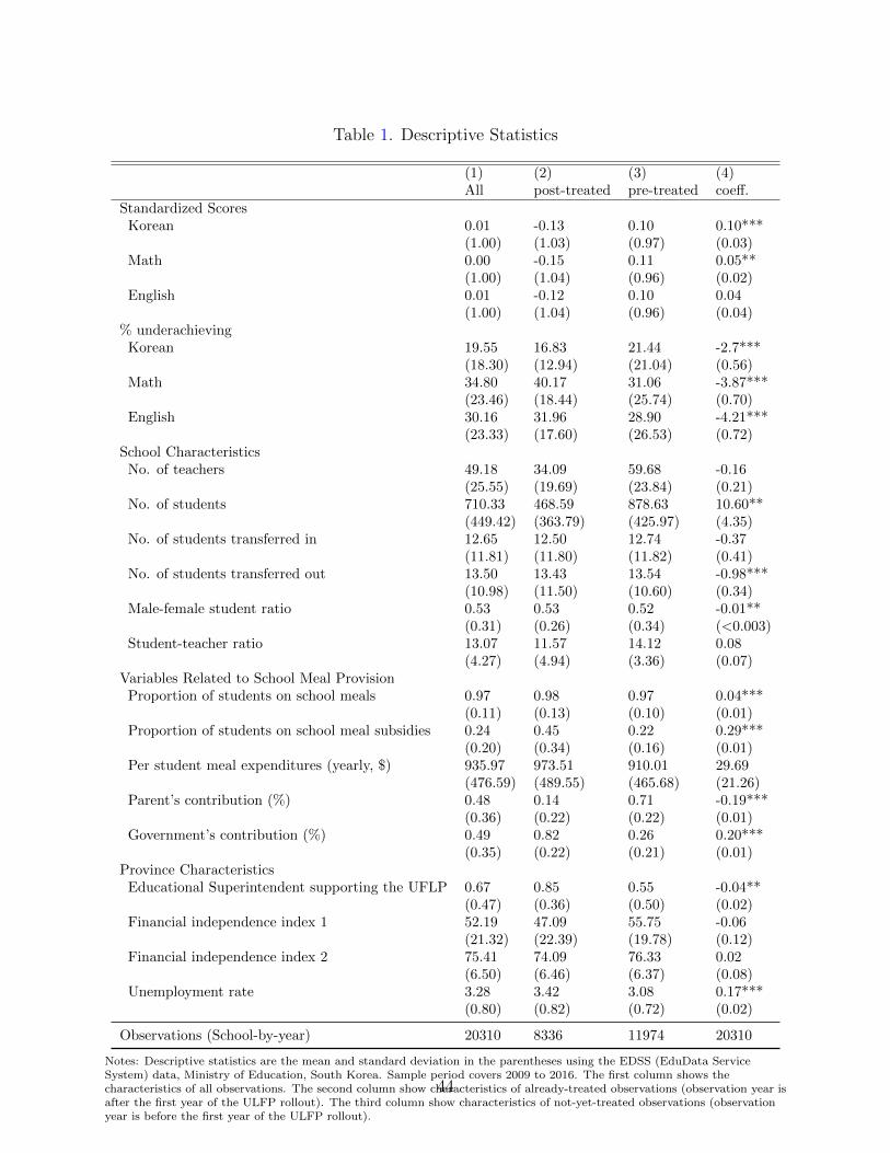
Table 1. Descriptive Statistics

(1) (2) (3) (4)All post-treated pre-treated coeff.

Standardized ScoresKorean 0.01 -0.13 0.10 0.10***

(1.00) (1.03) (0.97) (0.03)Math 0.00 -0.15 0.11 0.05**

(1.00) (1.04) (0.96) (0.02)English 0.01 -0.12 0.10 0.04

(1.00) (1.04) (0.96) (0.04)% underachieving

Korean 19.55 16.83 21.44 -2.7***(18.30) (12.94) (21.04) (0.56)

Math 34.80 40.17 31.06 -3.87***(23.46) (18.44) (25.74) (0.70)

English 30.16 31.96 28.90 -4.21***(23.33) (17.60) (26.53) (0.72)

School CharacteristicsNo. of teachers 49.18 34.09 59.68 -0.16

(25.55) (19.69) (23.84) (0.21)No. of students 710.33 468.59 878.63 10.60**

(449.42) (363.79) (425.97) (4.35)No. of students transferred in 12.65 12.50 12.74 -0.37

(11.81) (11.80) (11.82) (0.41)No. of students transferred out 13.50 13.43 13.54 -0.98***

(10.98) (11.50) (10.60) (0.34)Male-female student ratio 0.53 0.53 0.52 -0.01**

(0.31) (0.26) (0.34) (<0.003)Student-teacher ratio 13.07 11.57 14.12 0.08

(4.27) (4.94) (3.36) (0.07)Variables Related to School Meal Provision

Proportion of students on school meals 0.97 0.98 0.97 0.04***(0.11) (0.13) (0.10) (0.01)

Proportion of students on school meal subsidies 0.24 0.45 0.22 0.29***(0.20) (0.34) (0.16) (0.01)

Per student meal expenditures (yearly, $) 935.97 973.51 910.01 29.69(476.59) (489.55) (465.68) (21.26)

Parent’s contribution (%) 0.48 0.14 0.71 -0.19***(0.36) (0.22) (0.22) (0.01)

Government’s contribution (%) 0.49 0.82 0.26 0.20***(0.35) (0.22) (0.21) (0.01)

Province CharacteristicsEducational Superintendent supporting the UFLP 0.67 0.85 0.55 -0.04**

(0.47) (0.36) (0.50) (0.02)Financial independence index 1 52.19 47.09 55.75 -0.06

(21.32) (22.39) (19.78) (0.12)Financial independence index 2 75.41 74.09 76.33 0.02

(6.50) (6.46) (6.37) (0.08)Unemployment rate 3.28 3.42 3.08 0.17***

(0.80) (0.82) (0.72) (0.02)

Observations (School-by-year) 20310 8336 11974 20310

Notes: Descriptive statistics are the mean and standard deviation in the parentheses using the EDSS (EduData ServiceSystem) data, Ministry of Education, South Korea. Sample period covers 2009 to 2016. The first column shows thecharacteristics of all observations. The second column show characteristics of already-treated observations (observation year isafter the first year of the ULFP rollout). The third column show characteristics of not-yet-treated observations (observationyear is before the first year of the ULFP rollout).

44

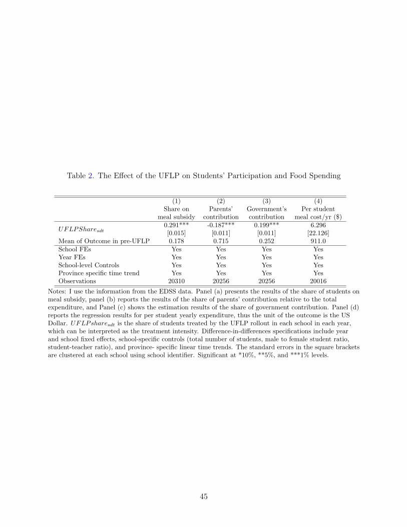
Table 2. The Effect of the UFLP on Students’ Participation and Food Spending

(1)Share on

meal subsidy

(2)Parents’

contribution

(3)Government’scontribution

(4)Per student

meal cost/yr ($)

UFLPSharesdt0.291***[0.015]

-0.187***[0.011]

0.199***[0.011]

6.296[22.126]

Mean of Outcome in pre-UFLP 0.178 0.715 0.252 911.0School FEs Yes Yes Yes YesYear FEs Yes Yes Yes YesSchool-level Controls Yes Yes Yes YesProvince specific time trend Yes Yes Yes YesObservations 20310 20256 20256 20016

Notes: I use the information from the EDSS data. Panel (a) presents the results of the share of students onmeal subsidy, panel (b) reports the results of the share of parents’ contribution relative to the totalexpenditure, and Panel (c) shows the estimation results of the share of government contribution. Panel (d)reports the regression results for per student yearly expenditure, thus the unit of the outcome is the USDollar. UFLPsharesdt is the share of students treated by the UFLP rollout in each school in each year,which can be interpreted as the treatment intensity. Difference-in-differences specifications include yearand school fixed effects, school-specific controls (total number of students, male to female student ratio,student-teacher ratio), and province- specific linear time trends. The standard errors in the square bracketsare clustered at each school using school identifier. Significant at *10%, **5%, and ***1% levels.

45

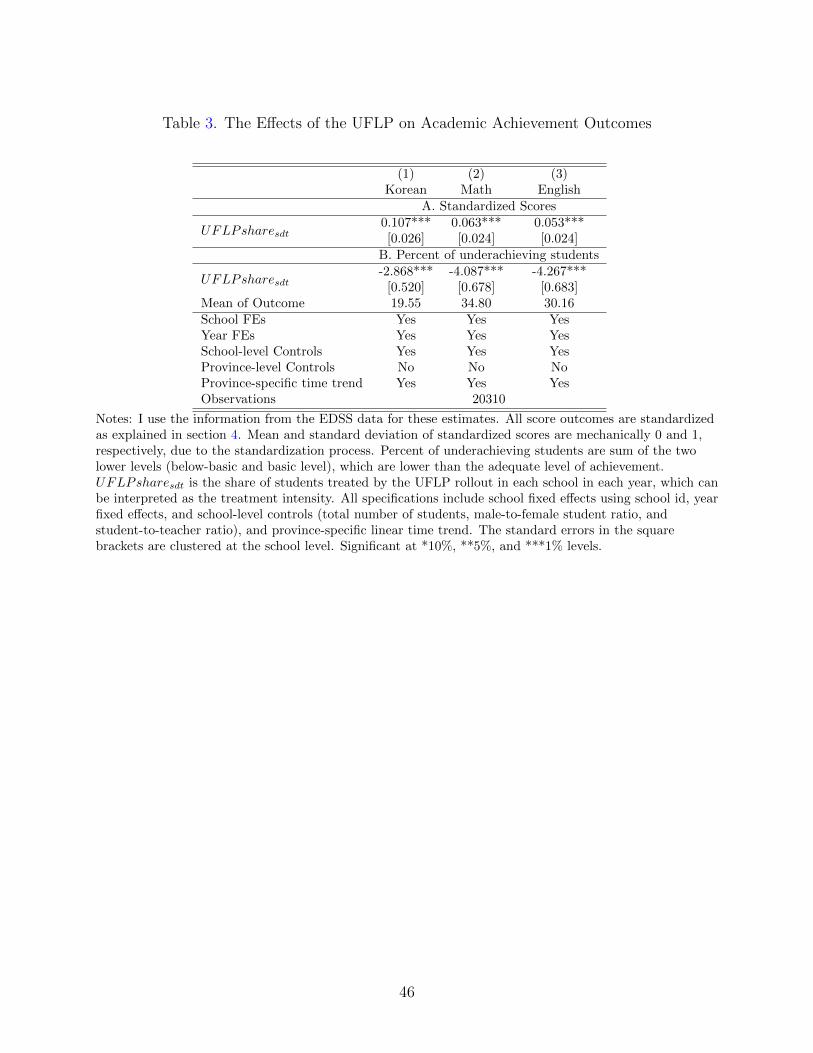
Table 3. The Effects of the UFLP on Academic Achievement Outcomes

(1)Korean

(2)Math

(3)English

A. Standardized Scores

UFLPsharesdt0.107***[0.026]

0.063***[0.024]

0.053***[0.024]

B. Percent of underachieving students

UFLPsharesdt-2.868***

[0.520]-4.087***

[0.678]-4.267***

[0.683]Mean of Outcome 19.55 34.80 30.16School FEs Yes Yes YesYear FEs Yes Yes YesSchool-level Controls Yes Yes YesProvince-level Controls No No NoProvince-specific time trend Yes Yes YesObservations 20310

Notes: I use the information from the EDSS data for these estimates. All score outcomes are standardizedas explained in section 4. Mean and standard deviation of standardized scores are mechanically 0 and 1,respectively, due to the standardization process. Percent of underachieving students are sum of the twolower levels (below-basic and basic level), which are lower than the adequate level of achievement.UFLPsharesdt is the share of students treated by the UFLP rollout in each school in each year, which canbe interpreted as the treatment intensity. All specifications include school fixed effects using school id, yearfixed effects, and school-level controls (total number of students, male-to-female student ratio, andstudent-to-teacher ratio), and province-specific linear time trend. The standard errors in the squarebrackets are clustered at the school level. Significant at *10%, **5%, and ***1% levels.

46

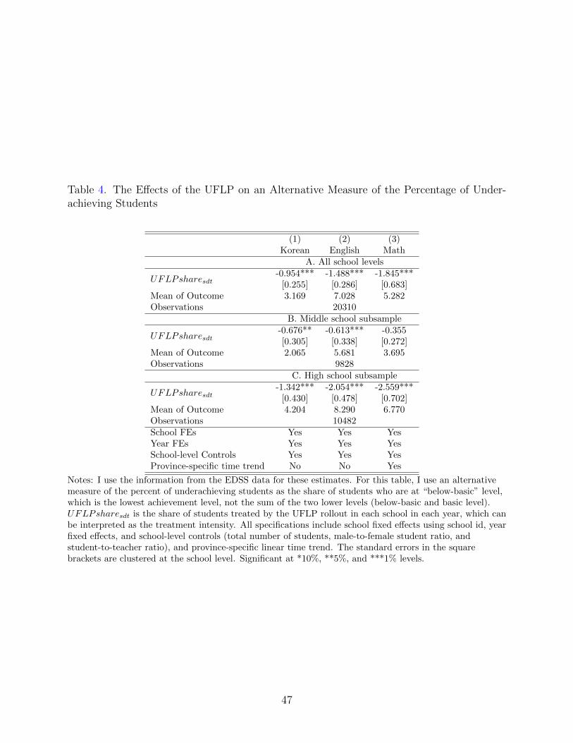
Table 4. The Effects of the UFLP on an Alternative Measure of the Percentage of Under-achieving Students

(1)Korean

(2)English

(3)Math

A. All school levels

UFLPsharesdt-0.954***

[0.255]-1.488***

[0.286]-1.845***

[0.683]Mean of Outcome 3.169 7.028 5.282Observations 20310

B. Middle school subsample

UFLPsharesdt-0.676**[0.305]

-0.613***[0.338]

-0.355[0.272]

Mean of Outcome 2.065 5.681 3.695Observations 9828

C. High school subsample

UFLPsharesdt-1.342***

[0.430]-2.054***

[0.478]-2.559***

[0.702]Mean of Outcome 4.204 8.290 6.770Observations 10482School FEs Yes Yes YesYear FEs Yes Yes YesSchool-level Controls Yes Yes YesProvince-specific time trend No No Yes

Notes: I use the information from the EDSS data for these estimates. For this table, I use an alternativemeasure of the percent of underachieving students as the share of students who are at “below-basic” level,which is the lowest achievement level, not the sum of the two lower levels (below-basic and basic level).UFLPsharesdt is the share of students treated by the UFLP rollout in each school in each year, which canbe interpreted as the treatment intensity. All specifications include school fixed effects using school id, yearfixed effects, and school-level controls (total number of students, male-to-female student ratio, andstudent-to-teacher ratio), and province-specific linear time trend. The standard errors in the squarebrackets are clustered at the school level. Significant at *10%, **5%, and ***1% levels.

47

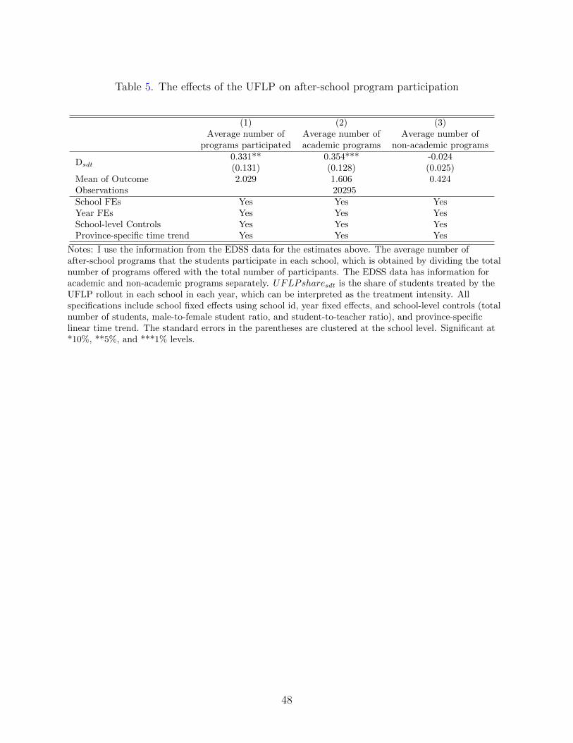
Table 5. The effects of the UFLP on after-school program participation

(1)Average number of

programs participated

(2)Average number ofacademic programs

(3)Average number of

non-academic programs

Dsdt0.331**(0.131)

0.354***(0.128)

-0.024(0.025)

Mean of Outcome 2.029 1.606 0.424Observations 20295School FEs Yes Yes YesYear FEs Yes Yes YesSchool-level Controls Yes Yes YesProvince-specific time trend Yes Yes Yes

Notes: I use the information from the EDSS data for the estimates above. The average number ofafter-school programs that the students participate in each school, which is obtained by dividing the totalnumber of programs offered with the total number of participants. The EDSS data has information foracademic and non-academic programs separately. UFLPsharesdt is the share of students treated by theUFLP rollout in each school in each year, which can be interpreted as the treatment intensity. Allspecifications include school fixed effects using school id, year fixed effects, and school-level controls (totalnumber of students, male-to-female student ratio, and student-to-teacher ratio), and province-specificlinear time trend. The standard errors in the parentheses are clustered at the school level. Significant at*10%, **5%, and ***1% levels.

48

Appendices

A Literature Review

A considerable body of literature investigated the relationship between nutrition and aca-demic achievement, especially in developing countries where malnutrition is a prevalentproblem. Earlier studies that established this nutrition-learning channel are summarizedin Glewwe and Miguel (2007) and in Alderman and Bundy (2012). Some of these studiesuse exogenous shocks such as policy interventions to provide better access to food, civil war,and drought to examine the differences in educational outcomes such as enrollment, highschool graduation rate, and years of schooling.

A strand of studies found that changes in school meal nutrition can be linked to students’academic achievement in developed countries. For example, there were policy changes in theUS and UK that provided healthier school meals to students, and studies have found thathealthier school meals improve academic achievement outcomes (Andersen, Gallagher, andRitchie 2017; Belot and James 2011). Regarding the impact of caloric content, Figlio andWinicki (2005) find that increased caloric content is linked to increased standardized testscores in the US, but McEwan (2013) finds no such link in Chile.

Several studies examined the effects of the expanded access to school meals on educa-tional outcomes, and general findings suggest that expanded access to school meals leads tomore school lunch participation, better nutrition and better academic achievement. Manycountries provide subsidized school meals for students with lower family incomes (OECD2012) to assist students from lower income families. Bartfield and Ahn (2011), Frisvold(2015), and Schwartz and Rothbart (2020), Ruffini (2020) points out that improved nutri-tion is a key factor behind the improvement found in academic achievement. Still, not allof these studies can rule out the effects of increased incentives for students to attend school.Many studies point out increased attendance and enrollment (Hindrich 2010; Leos-Urbelet al. 2013; Imberman and Kugler 2014; Jayaraman and Simroth 2015; Chakraborty andJayaraman 2019).

Since many countries provide means-tested subsidies for school lunches, there are concernsregarding the association between free lunch status and stigma. There exists abundantanecdotal evidence and correlation between stigma and take-up of the means-tested subsidy(Glantz and Long 1994; Pogash 2008; Mirtcheva and Powell 2009; Sandman 2016). Notably,Yu, Lim and Kelly (2019) find suggestive evidence that the stigma associated with the means-tested lunch subsidy in Seoul, South Korea, is more notable in schools with a low percentageof students on lunch subsidy.

This paper provides suggestive evidence that the improved educational outcomes areassociated with the increased spending on educational inputs, specifically by increased par-ticipation in academic after-school programs. In the South Korean context, where moststudents receive lunch from their schools, expanded access to school meals create increaseddisposable income for parents. These results can be linked to the “mental accounting” inbehavioral economics, where they focus on the evidence against the complete fungibility ofmoney. People often allocate funds for specific purposes (such as housing, food, or children’seducation), and the categorized budget often restricts money to move across different pur-poses of expenditure. People can experience disutility by exceeding the categorical budget,

A1

and Thaler (1990, 1998, and 1999)’s work provides pertinent examples. On top of the incomeeffect, mental accounting provides grounds for expecting an even greater impacts on edu-cation expenditure, especially because parents clearly knew that the increased disposableincome (if they were not participating in the means-tested lunch subsidy) was the schoollunch fee saved due to the UFLP. Gouldner (1960) documented that the benefit recipientsare likely to be nudged towards the suggested uses of the benefit. These findings suggestthat the saved lunch fees would be spent more on children’s education.

Large body of empirical literature supports the incomplete fungiblility of money. Lund-berg, Pollak, and Wales (1997) find evidence that benefits labeled for children in the UKhad greater tendency to be spent on children.45 More recently, Jones et al. (2019) andHener (2017)’s results suggest that the benefits earmarked for children leads to increasedhousehold expenses on direct education inputs and day-to-day items that are likely to be forthe children.

There are two other studies which studies the effect of the UFLP. As the UFLP increasesthe share of students on meal subsidy, Altindag et al. (2020) examine the impacts of theincreased share on school misbehavior outcomes, and Baek et al. (2019) investigate how itaffects the physical ability of students. Altindag et al. (2020) find reduction in misbehavior,but Baek et al. (2019) do not find changes in students’ physical aptitude.46 47

B South Korean School System

In this subsection, I briefly describe the school system in South Korea. Students spend sixyears in elementary school, three years in middle school, and three years in high school.This 6-3-3 system is kept regardless of the school type or regions, and skipping a graderarely happens. Elementary school is from grade 1 (age 7) to grade 6 (age 12). Startingfrom the first grade, students have lunch at school. Elementary school education has beencompulsory since 1952, and all students are admitted to schools by lottery system withinthe school districts.

After graduating from elementary school, students go to middle school. Middle schooleducation became compulsory by law in 1984, and in 1999, the middle school enrollment ratewas 99.9 percent. More than 99 percent of the middle schools are general middle schools,which are subject to the admission by lottery within the school district. Less than onepercent of middle schools are for students with specialties in art, music, or physical ability(to be professional athletes). These schools have their own entrance exams to measure the

45Lundberg, Pollak and Wales (1997) and Kenney (2008) also points out that this phenomenon is proneto be greater if the child benefits are controlled by the mother. Before the UFLP, school lunch fees weregenerally paid by mothers as anecdotal evidence (Ryu et al. 2011) and research on household financialmanagement (Lee et al. 2008).

46In order to show that there was no selection of schools based on the scores into the program, Altindaget al. (2020) used the standardized scores as outcomes and conclude that the UFLP has no effects on thestandardized scores. The main difference from this paper’s approach to Altindag et al. (2020)’s approach isthe identifying variation. This paper utilizes the UFLP rollout information, and Altindag et al. (2020) usesthe share of students on school meal subsidy, which is affected by the UFLP rollout. The share of studentson school meal subsidy increased due to the UFLP, and Altindag et al. (2020) defined the schools as treatedby the UFLP if this share is greater than 0.9 in each school. See section 4 for more detail.

47Replication results of these two papers are summarized in appendix section E.

A2

students’ artistic or physical ability but not their academic achievement.The high school enrollment rate is over 99 percent since 2002 (OECD 2021). High schools

can be categorized into three types. Roughly 88 percent of the schools are for the studentswho pursue post-secondary education, including general high schools, foreign language highschools, and science high schools. General high schools consist of approximately 80 percentof all high schools. Foreign language and science high schools select students among theapplicants by their own exams or interviews, but the difficulty and the evaluation procedureof the exam are also subject to a centralized guideline. Arts and physical high schoolsconsist of less than 2 percent of the total high schools, and they also admit a selectedgroup of students who passed their exams. The rest are vocational high schools, includingtechnical high schools, commercial high schools, fishery high schools, and agricultural highschools. The University enrollment rate is less than 40 percent among these vocationalschools, counting for both technical and university degrees.

One feature to note is that South Korea has a very centralized education system regard-less of the school type. Almost all school types share common regulations regarding thecurriculum, textbooks, school facilities, and teacher quality.48 Foreign language high schoolsand science high schools have entrance exams, and average achievement in these schools canbe higher than the general public. Still, these schools were not treated differently in termsof the universal free lunch program rollout.49

Between 2009 and 2016, all the third grade of middle school students and second grade ofhigh school students took the NAEA exam. Every elementary school student in sixth gradetook this test from 2009, but the government stopped this elementary school assessmentprocedure in 2013 and the only available outcome for elementary schools is the percentageof underachieving students. For the comparability of the regression results, I focus on themiddle schools and high schools, which have both the scores and the percentage information.The data availability for each school level is summarized in figure A.2.

Province-level unemployment rate is obtained from Korean Statistical Information Ser-vice (KOSIS), and is generally higher among the post-treated observations.50

48Public school teachers need to pass the national teaching license exam as the first class, but privateschools can hire teachers with a second-class teaching license. Teachers with second class teaching licensesmust satisfy two requirements (at least three years of teaching experience and passing a training program) toobtain the first-class license. All public school teachers are subject to the rotation to another public schoolafter five years.

49Private elementary schools in Seoul and Busan were treated later than the public elementary schools,but these are less than 1 percent of the total elementary schools in each city.

50See https://kosis.kr/statHtml/statHtml.do?orgId=101&tblId=INH 1DA7104S&conn path=I3 formore information.

A3

C Instrumental Variables Regression

In this subsection, I discuss the instrumental variable regression model. The Universal FreeLunch Program is intended to increase the share of the students on lunch subsidy ultimatelyto one hundred percent. However, the share might be increasing or decreasing due to otherfactors such as neighborhood characteristics and regional business cycle. Previous studiessuch as Altindag et al. (2020) and Baek et al. (2019) used the share of the studentson meal subsidy as the treatment variable, and thus subject to the bias originated fromthe variations other than the UFLP.51 EDSS data do not provide the information of eachschool being treated by the Universal Free Lunch Program or not, but it provides the shareof students receiving a subsidized meal. I use the Universal Free Lunch Program rolloutinformation (UFLPSharesdt) to instrument the share of students on a subsidized meal,denoted as Sharesdt. The value of Sharesdt also ranges from 0 to 1 as UFLPSharesdt. Ifthis measurement error is pervasive in Sharesdt, using only the variation of Sharesdt thatwas originated from the program rollout information would measure the causal effect of theprogram.

Two-stage least squares (2SLS) regression captures the variation in Sharesdt that is as-sociated with the variation of the program rollout. This first stage regression of regressingSharesdt on the program rollout information measured by UFLPSharesdt prevents the po-tential endogeneity or omitted variable bias issues. The two-stage least squares regressionequations can be described as follows:

Ysdt = α Sharesdt + ΓXsdt + ΠZdt + µs + µt + ωsdt (5)

Sharesdt = ρUFLPSharesdt + ΘXsdt + ΥZdt + ηs + ηt + νsdt (6)

where Ysdt is the academic achievement outcome of school s in province d in year t. Xsdt

includes school-level controls, and Zdt includes provincial level controls as in the baselinespecification. µs is school fixed effects, µt is year fixed effects. ωsdt is the error term.Sharesdt is the fitted value of Sharesdt derived from equation (4). Equation (4) is the firststage regression equation that captures the relationship between the Universal Free LunchProgram rollout (UFLPSharesdt) and the share of students on meal subsidy (Sharesdt).The fitted value of this first stage regression is the treatment variable of interest, and α hasa different interpretation compared to the interpretation of β in the baseline regression. Byincreasing the share of students who are on meal subsidy by 10 percentage points, it resultsin the 10 × α percentage point increase of the outcome of interest. ηs is school fixed effects,

51There is one more possibility that the schools are reporting other information than the share of the lunchsubsidy. According to several provincial offices of the Ministry of education, if schools that are supposed tobe fully treated (when Dsdt = 1) are not reporting almost one hundred percent of the Sharesdt, they mightbe reporting the share of students on subsidized snacks or dinner. It is common for high schools in SouthKorea to provide dinner since the students are likely to remain in school to study more after the regular classtime. Snacks are relatively more prevalent, and the most common form is fresh white milk. This white milksnack started in 1981 and was mandatory in the 1980s but gradually changed towards providing it to only theones who subscribe to this. Even after the lunch meal became free, subsidy for milk and other snacks is stillbased on the means-tested procedure. In the late 2010s, roughly 50 percent of students were participating inthe milk snack program. In 2017, fruit snack programs were implemented, but not as broadly or frequentlyas milk snack program.

A4

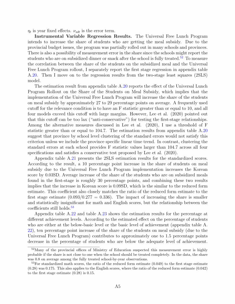
ηt is year fixed effects. νsdt is the error term.Instrumental Variable Regression Results. The Universal Free Lunch Program

intends to increase the share of students who are getting the meal subsidy. Due to theprovincial budget issues, the program was partially rolled out in many schools and provinces.There is also a possibility of measurement error in the share since the schools might report thestudents who are on subsidized dinner or snack after the school is fully treated.52 To measurethe correlation between the share of the students on the subsidized meal and the UniversalFree Lunch Program rollout, I separately report the first stage regression in appendix tableA.20. Then I move on to the regression results from the two-stage least squares (2SLS)model.

The estimation result from appendix table A.20 reports the effect of the Universal LunchProgram Rollout on the Share of the Students on Meal Subsidy, which implies that theimplementation of the Universal Free Lunch Program will increase the share of the studentson meal subsidy by approximately 27 to 29 percentage points on average. A frequently usedcutoff for the relevance condition is to have an F statistic greater than or equal to 10, and allfour models exceed this cutoff with large margins. However, Lee et al. (2020) pointed outthat this cutoff can be too lax (“anti-conservative”) for testing the first-stage relationships.Among the alternative measures discussed in Lee et al. (2020), I use a threshold of Fstatistic greater than or equal to 104.7. The estimation results from appendix table A.20suggest that province by school level clustering of the standard errors would not satisfy thiscriterion unless we include the province specific linear time trend. In contrast, clustering thestandard errors at each school provides F statistic values larger than 104.7 across all fourspecifications and satisfies a conservative test proposed by Lee et al. (2020).

Appendix table A.21 presents the 2SLS estimation results for the standardized scores.According to the result, a 10 percentage point increase in the share of students on mealsubsidy due to the Universal Free Lunch Program implementation increases the Koreanscore by 0.03SD. Average increase of the share of the students who are on subsidized mealsfound in the first-stage is roughly 30 percentage points, and combining these two resultsimplies that the increase in Korean score is 0.09SD, which is the similar to the reduced formestimate. This coefficient also closely matches the ratio of the reduced form estimate to thefirst stage estimate (0.093/0.277 = 0.336). The impact of increasing the share is smallerand statistically insignificant for math and English scores, but the relationship between thecoefficients still holds.53

Appendix table A.22 and table A.23 shows the estimation results for the percentage atdifferent achievement levels. According to the estimated effect on the percentage of studentswho are either at the below-basic level or the basic level of achievement (appendix table A.22), ten percentage point increase of the share of the students on meal subsidy (due to theUniversal Free Lunch Program) contributes to approximately one to 1.5 percentage pointsdecrease in the percentage of students who are below the adequate level of achievement.

52Many of the provincial offices of Ministry of Education suspected this measurement error is highlyprobable if the share is not close to one when the school should be treated completely. In the data, the sharewas 0.8 on average among the fully treated school-by-year observations.

53For standardized math scores, the ratio of the reduced form estimate (0.049) to the first stage estimate(0.28) was 0.175. This also applies to the English scores, where the ratio of the reduced form estimate (0.042)to the first stage estimate (0.28) is 0.15.

A5

These effects span from 40 to 50 percent decrease compared to the mean. The estimatedeffect of UFLP in terms of decreasing the percentage of students who falls behind exhibitslarger impact in decreasing the percentage of students at the below-basic level of achievement,which are presented in appendix table A.23.

A6

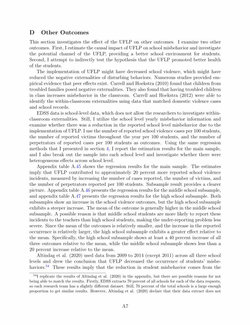
D Other Outcomes

This section investigates the effect of the UFLP on other outcomes. I examine two otheroutcomes. First, I estimate the causal impact of UFLP on school misbehavior and investigatethe potential channel of the UFLP, providing a better school environment for students.Second, I attempt to indirectly test the hypothesis that the UFLP promoted better healthof the students.

The implementation of UFLP might have decreased school violence, which might havereduced the negative externalities of disturbing behaviors. Numerous studies provided em-pirical evidence that peer effects exist. Carrell and Hoekstra (2010) found that children fromtroubled families posed negative externalities. They also found that having troubled childrenin class increases misbehavior in the classroom. Carrell and Hoekstra (2012) were able toidentify the within-classroom externalities using data that matched domestic violence casesand school records.

EDSS data is school-level data, which does not allow the researchers to investigate within-classroom externalities. Still, I utilize the school level yearly misbehavior information andexamine whether there was a reduction in the reported school level misbehavior due to theimplementation of UFLP. I use the number of reported school violence cases per 100 students,the number of reported victims throughout the year per 100 students, and the number ofperpetrators of reported cases per 100 students as outcomes. Using the same regressionmethods that I presented in section 4, I report the estimation results for the main sample,and I also break out the sample into each school level and investigate whether there wereheterogeneous effects across school level.

Appendix table A.45 shows the regression results for the main sample. The estimatesimply that UFLP contributed to approximately 20 percent more reported school violenceincidents, measured by increasing the number of cases reported, the number of victims, andthe number of perpetrators reported per 100 students. Subsample result provides a clearerpicture. Appendix table A.46 presents the regression results for the middle school subsample,and appendix table A.47 presents the regression results for the high school subsample. Bothsubsamples show an increase in the school violence outcomes, but the high school subsampleexhibits a steeper increase. The mean of the outcome is generally higher in the middle schoolsubsample. A possible reason is that middle school students are more likely to report theseincidents to the teachers than high school students, making the under-reporting problem lesssevere. Since the mean of the outcomes is relatively smaller, and the increase in the reportedoccurrence is relatively larger, the high school subsample exhibits a greater effect relative tothe mean. Specifically, the high school subsample shows at least a 40 percent increase of allthree outcomes relative to the mean, while the middle school subsample shows less than a20 percent increase relative to the mean.

Altindag et al. (2020) used data from 2009 to 2014 (except 2011) across all three schoollevels and drew the conclusion that UFLP decreased the occurrence of students’ misbe-haviors.54 These results imply that the reduction in student misbehavior comes from the

54I replicate the results of Altindag et al. (2020) in the appendix, but there are possible reasons for notbeing able to match the results. Firstly, EDSS extracts 70 percent of all schools for each of the data requests,so each research team has a slightly different dataset. Still, 70 percent of the total schools is a large enoughproportion to get similar results. However, Altindag et al. (2020) declare that their data extract does not

A7

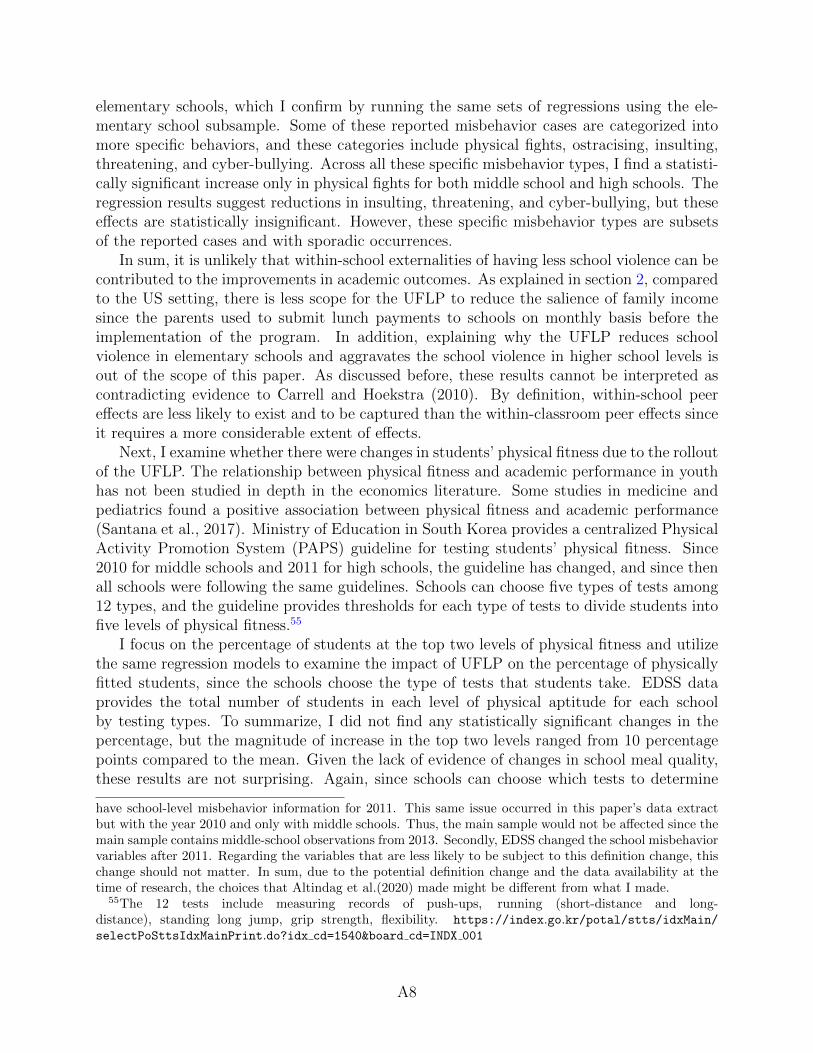
elementary schools, which I confirm by running the same sets of regressions using the ele-mentary school subsample. Some of these reported misbehavior cases are categorized intomore specific behaviors, and these categories include physical fights, ostracising, insulting,threatening, and cyber-bullying. Across all these specific misbehavior types, I find a statisti-cally significant increase only in physical fights for both middle school and high schools. Theregression results suggest reductions in insulting, threatening, and cyber-bullying, but theseeffects are statistically insignificant. However, these specific misbehavior types are subsetsof the reported cases and with sporadic occurrences.

In sum, it is unlikely that within-school externalities of having less school violence can becontributed to the improvements in academic outcomes. As explained in section 2, comparedto the US setting, there is less scope for the UFLP to reduce the salience of family incomesince the parents used to submit lunch payments to schools on monthly basis before theimplementation of the program. In addition, explaining why the UFLP reduces schoolviolence in elementary schools and aggravates the school violence in higher school levels isout of the scope of this paper. As discussed before, these results cannot be interpreted ascontradicting evidence to Carrell and Hoekstra (2010). By definition, within-school peereffects are less likely to exist and to be captured than the within-classroom peer effects sinceit requires a more considerable extent of effects.

Next, I examine whether there were changes in students’ physical fitness due to the rolloutof the UFLP. The relationship between physical fitness and academic performance in youthhas not been studied in depth in the economics literature. Some studies in medicine andpediatrics found a positive association between physical fitness and academic performance(Santana et al., 2017). Ministry of Education in South Korea provides a centralized PhysicalActivity Promotion System (PAPS) guideline for testing students’ physical fitness. Since2010 for middle schools and 2011 for high schools, the guideline has changed, and since thenall schools were following the same guidelines. Schools can choose five types of tests among12 types, and the guideline provides thresholds for each type of tests to divide students intofive levels of physical fitness.55

I focus on the percentage of students at the top two levels of physical fitness and utilizethe same regression models to examine the impact of UFLP on the percentage of physicallyfitted students, since the schools choose the type of tests that students take. EDSS dataprovides the total number of students in each level of physical aptitude for each schoolby testing types. To summarize, I did not find any statistically significant changes in thepercentage, but the magnitude of increase in the top two levels ranged from 10 percentagepoints compared to the mean. Given the lack of evidence of changes in school meal quality,these results are not surprising. Again, since schools can choose which tests to determine

have school-level misbehavior information for 2011. This same issue occurred in this paper’s data extractbut with the year 2010 and only with middle schools. Thus, the main sample would not be affected since themain sample contains middle-school observations from 2013. Secondly, EDSS changed the school misbehaviorvariables after 2011. Regarding the variables that are less likely to be subject to this definition change, thischange should not matter. In sum, due to the potential definition change and the data availability at thetime of research, the choices that Altindag et al.(2020) made might be different from what I made.

55The 12 tests include measuring records of push-ups, running (short-distance and long-distance), standing long jump, grip strength, flexibility. https://index.go.kr/potal/stts/idxMain/selectPoSttsIdxMainPrint.do?idx cd=1540&board cd=INDX 001

A8

these aptitude levels, this measure’s comparability across schools is unclear.

A9

E Replication of Altindag et al. (2020) and Baek et al. (2019)

There are two possible reasons for my results to be different from the results of Altindag etal. (2020) and Baek et al. (2019) who investigated the effects of the UFLP on various school-level outcomes. Specifically, Altindag et al. (2020) reports that they find no statisticallysignificant increase in standardized scores. The first reason is the longer sample period thatI am using (I have two more years than Altindag et al. (2020), and 4 or 5 more yearsthan Baek et al. (2019)). The second reason is due to the different definition of treatment.Still, even though the value of the treatment is different, if the both treatment definition isdetermined by the same underlying variation, then the treatment effects should be similarlyestimated. This purpose of this subsection is to provide evidence to determine which one ofthese two reasons is more likely to be the cause of the different results that I am finding. Iclosely follow the sample restrictions that these two papers make, and see if the regressionresults are similar.

Replication of Altindag et al. (2020). Altindag et al. (2020) examined the effect ofthe UFLP on student misbehavior outcomes, mainly number of the cases reported, numberof offenders, number of victims. They found that the UFLP contributed to large reduction(largely 50 percent of the mean) in student misbehavior. They used the data from 2009to 2014 except for 2011 since the information was all missing for year 2011. I find thatsummary statistics such as school characteristics and number of cases are very close to whatthey are reporting. I follow their regression specification use two treatment definitions,following Altindag et al. (2020), and using the UFLP rollout information. When I use thetreatment definition of Altindag et al. (2020), the regression results are similar to thosereported in Altindag et al. (2020). In contrast, when I use the UFLP rollout information astreatment, the results differ in terms of magnitude, statistical significance, and the signs ofthe coefficients.

Replication of Baek et al. (2019). Baek et al.(2019) investigated the effects ofthe UFLP on students’ physical fitness. Students are classified into 5 levels of physicalfitness, which is measured with physical performance on various types of exercises, includingpush-ups, 100-meter running, etc. Their outcome measure is the share of students who areclassified as level 1 and 2 per 100 students, which represents the share of students withhigh fitness in each school in each year. They found no significant impact on the share ofstudents with high physical aptitude due to the implementation of the universal free lunchprogram. Again, I find that the summary statistics of dependent and control variables arevery similar. I also find similar results with that of Baek et al. (2019) when I use thetreatment definition of theirs. However, using the UFLP implementation information astreatment, the regression estimates contradicts to those reported in Baek et al. (2019) interms of magnitude, statistical significance, and the signs of the coefficients.

This replication exercise cannot perfectly match the regression results of these two otherstudies, as the EDSS creates different extract for each of the projects. Still, using the samesample resulted in contradicting results depending on which treatment definition that Iuse. This suggests that the UFLP implementation information and the treatment definitionof Altindag et al. (2020) and Baek et al. (2019) are determined by different underlyingvariations.

A10

F Cost-Effectiveness of the UFLP

In this section, I discuss the cost-effectiveness of the UFLP using the estimated impact onthe standardized scores following Dhaliwal et al. (2013). Cost-effectiveness can be describedas effects that a program brings relative to the cost incurred. One advantage of the cost-effectiveness analysis is that the program’s estimated impacts are easily comparable acrossdifferent countries and years. Moreover, the unit of the effect is the same as the outcomeof interest. Thus, the cost-effectiveness analysis does not require an assumption to be madeabout the benefits’ monetary value (which can differ across readers and policymakers) in-duced by the effect. Compared to the case of cost-benefit analysis, this is a convenientadvantage. However, due to this program’s nature (since it is not a field experiment), in-formation on many types of costs are not available. I summarize the procedure to calculatethe cost and the effectiveness of the UFLP while providing the limitations and assumptionsthat are made to calculate the cost-effectiveness estimates that I find.

Dhaliwal et al. (2013) provide detailed steps to calculate the cost-effectiveness of aprogram. In terms of the program’s effect, they advise considering only the statisticallysignificant effects at 10 percent level or better. The suggested calculation of the total impactof a program differs slightly by the design of the program. In terms of the Intent-to-Treateffects (ITT), the program’s total impact can be derived by multiplying the estimated Intent-To-Treat effect by the corresponding sample size. For the estimated Intent-to-treat effects,I use the estimates obtained by using the preferred specification (which includes schooland year fixed effects, time-varying school-level characteristics, and province-specific lineartime trend). The estimated impacts using this specification are statistically significant at a10 percent level or better across all three subjects. For the sample size, I use the affectedpopulation by using the treatment intensity (UFLPSharesdt) in each school across the yearsavailable in the sample.56 I use a 10 percent social discount rate of the effects to aggregatethe effects of the UFLP over the years to reflect the social opportunity cost of capital andconvert the effect in the value of the year 2020.57

Due to the data limitation, quantifying the cost of the UFLP requires more assumptions.I use the governmentsa contribution for school lunches as the cost of the UFLP (which isalso utilized to derive the share of governments’ contribution for school lunches). Ideally,the cost calculation would take only the cost additionally incurred by implementing theprogram (“cost at the margin”). But the EDSS data do not have information on how thesefunds are spent. Thus, this cost might include the costs that are not ideally included in costcalculation (such as cost for equipment that would already be present without the UFLP)and might not include the costs that should be included (such as administrative costs). Theuniversal provision would not require means-testing to determine eligibility, which wouldlikely decrease the administrative cost. However, since almost all students are already gettinglunch from their schools before the initiation of the UFLP (with some portion of students

56According to Dhaliwal et al. (2013), the program duration should also be multiplied. Nevertheless, sincethis paper estimates the intent-to-treat effect over the post-treatment period, multiplying the duration seemsmore appropriate for the Treatment on the Treated (ToT).

57According to Zhuang et al. (2007), the applicable social discount rate for several European countries(including Germany, Norway, UK, France) is 4 percent. For the US, it is 7 percent and a 10 percent rate forCanada. Asian Development Bank utilizes a 10 to 12 percent discount rate (Zhuang et al. 2007; Dhaliwalet al., 2013).

A11

on the means-tested lunch subsidy), this cost estimate is likely to be an overestimation. Tomake the cost into the US dollar unit in 2020, I use a 10 percent discount rate, averageannual inflation rate, and average annual exchange rate.58

The effectiveness-cost ratio is obtained by dividing the total impact by the total costestimates.59 The results suggest that per annual cost per student (approximately 600 to720 US dollars), the effect size spans from 0.075 SD to 0.091 SD for Korean, 0.044 SD to0.053 SD for Math, and 0.037 SD to 0.045 SD for English scores. According to Yeh (2010),the effectiveness-cost ratio estimates (converted to US dollar unit in 2020 with 10 percentdiscount rate) of various programs span from 0.000004 to 0.098 SD increase for readingand math scores.60 This leads to the conclusion that the UFLP is relatively cost-effectiveeven though it does not explicitly aim to raise student achievement. However, includingthe measurement error issues regarding the cost, the cost-effectiveness of the UFLP canhave limited generalizability. For example, if other countries were to adopt the program,depending on the institutional context, the cost to implement this program can be muchhigher than in South Korea. Since early 1990, almost 100 percent of students in SouthKorea received lunch through their schools, and thus the essential equipment and staffs toprovide lunch to all students were already in place. If this is not the case in other settings,the program’s cost increases and thus reduces the cost-effectiveness of the program.

58The annual inflation rate series is obtained from the US Bureau of Economic Analysis (2021), and theannual exchange rate is obtained from the University of Groningen and the University of California, Davis(2021). Both series are obtained via Federal Reserve Economic Data (FRED).

59One can also divide the total cost by the total impact to obtain the cost per additional unit of improve-ment of the outcome of interest, but for better comparability with other programs, I use the effect relativeto the cost measure.

60Table 1 of Yeh (2010) summarizes the effectiveness-cost ratios measured in 2006 USD. For these ratiosto be directly comparable with the cost-effectiveness of the UFLP, I used a 10 percent discount rate and anannual inflation rate of the US to convert these values. However, this still is not an accurate conversion into2020 US dollars since I do not have information on the program’s cost stream or effect stream over the years.

A12

G Difference-in-Differences with Different Treatment Timing

To consider the potential bias originated from the heterogeneous treatment effect, I imple-ment the estimator proposed by de Chaisemartin and D’Haultfoeuille (2020). This estimatoris one of the recent innovations in difference-in-differences that allow the researchers to re-flect heterogeneous effect and staggered adoption of treatment in the real setting. I use thesame main sample, a panel data of 70 percent stratified sample of middle schools from 2013to 2016 and high schools from 2009 to 2016, and apply de Chaisemartin and D’Haultfoeuille(2020)’s estimator (DIDM). The estimator of de Chaisemartin and D’Haultfoeuille (2020)allows control variables to be included and extends to nonbinary treatment. I present resultsfor two different cases in terms of the treatment definition. First is binary treatment, wherethe school is considered treated if a year of observation is equal to or greater than the firstyear that school is treated. This definition is comparable to the definition used in the eventstudy analyses. Second is the continuous treatment spanning from zero to one, with sharesof students affected by the UFLP as the value of treatment. This definition is the same asthe one used in the regression analyses.

Two way fixed effects estimated with OLS (βfe) can be decomposed into the weightedsums of the average treatment effects (ATE) in each group and each period (Borusyak andJaravel, 2017; de Chaisemartin and D’Haultfoeuille, 2020; Callaway and Sant’Anna, 2020;Goodman-Bacon, 2020; Sun and Abraham, 2020). To establish the extent of the bias comingfrom the negative weights, I report how many of these group-period combinations receivenegative weights and how much the negative weights are. Moreover, following the proof inde Chaisemartin and D’Haultfoeuille (2020), I test whether the homogenous treatment effectassumption holds or not by using the difference of the two-way fixed effect estimator (βfe)

and the first difference estimator (βfd). Then I move on to the DIDM estimates and discuss

the plausibility of a common trend assumption by using the placebo estimator (DIDplM)

proposed by de Chaisemartin and D’Haultfoeuille (2020).These placebo estimators are used as a criterion to select one among the four specifica-

tions that were utilized throughout the paper’s main analysis. This specification includesschool and year fixed effects, region-specific linear time trend, and school-specific controlvariables.61 This specification passes the common trend assumption test with two placeboestimates, which allows DIDM estimates to have causal interpretation across all three sub-jects. Thus, I focus on the results using this specification and report the estimates relatedto the Chaisemartin and D’Haultfoeuille (2020)’s method in appendix table A.26.

First I present the results with the binary treatment definition. According to the two-way fixed effect estimation result using the controls as specified above, 4019 among the 8172total group-period combinations have strictly negative weights. The sum of these negativeweights is equal to -0.231. Using the first difference, 3963 among the 8095 of all combinationsof ATT have strictly negative weights. This comprises roughly a half of all combinations,and the sum of all negative weights is equal to -0.443. These sums of negative weights areapplied to all three subjects, but the difference comes from the different group-period ATTs.Since the group-period ATTs are different across the subjects, this leads to different DIDM

estimates.

61This specification is reported in the third column of the regression result tables, in general.

A13

Even if the weights associated with group-period combinations for βfe are negative, if

the weights are uncorrelated with the ATEs conditional on the treatment, βfe can still berobust to heterogeneous treatment effects across group and periods. Similar logic also appliesto βfd as well. However, if the common trend assumption is true, these two assumptions

(one for βfe and one for βfd) cannot be satisfied jointly62. Thus, one can test whether βfeand βfd significantly differ and test the plausibility of the common trend assumption. First,t-statistics for each of the bootstrap sample in each cluster (by dividing the difference of thetwo estimates, βfe− βfd, with the standard deviation of the difference) is calculated, and byusing the average value of these statistics is used to determine the statistical significance.63

The numerical test result for Korea score suggests that (t-statistic = -0.680) the βfe (=0.082

with s.e. of 0.025, clustered at school id level) and βfd (=0.090 with s.e. of 0.033, clusteredat school id level) are not statistically significantly different, which does not casts doubt onthe homogenous treatment effect. Largely the same conclusion can be drawn with math andEnglish scores as well. For math scores, βfe (=0.041 with s.e. of 0.022, clustered at school id

level) and βfd (=0.024 with s.e. of 0.027, clustered at school id level) were not statisticallysignificantly different from zero with t-test statistic equal to -0.319. Similarly for Englishscores, βfe (=0.038 with s.e. of 0.022, clustered at school id level) and βfd (=0.019 with s.e.of 0.025, clustered at school id level) were not statistically significantly different from zerowith t-test statistic equal to 1.014. All βfe and βfd estimates are summarized in panel A ofappendix table A.26.64

Next, I move on to calculating the proposed estimator of de Chaisemartin and D’Haultfoeuille(2020), which is denoted by DIDM . In general, the DIDM estimates have a greater magni-tude than the two-way fixed effects estimates (βfe), which suggests that the two-way fixedeffect estimates are affected by modest negative bias. I use model specification with theschool fixed effects, year fixed effects and school level controls and all estimates are reportedin panel A of appendix table A.26. The estimated DIDM for Korean score is equal to 0.010which suggest 0.10 SD increase in Korean test scores with a standard error of 0.041. DIDM

estimates for math and English score implies the improvement of 0.052 SD and 0.045 SD,respectively. In sum, the bias of the two-way fixed effect estimators originated from theheterogeneous treatment effect is not severe to neither flip the sign nor severely underesti-mate the treatment effect of interest. This is also corroborated with the t-test results of thedifferences between FE estimates (βfe) and FD estimates (βfd).

The assumption that DIDM relies on to have a causal interpretation is a common trendassumption. The plausibility of this assumption can be tested by using the placebo estimator,DIDpl

M . This placebo estimator compares the change of the mean outcome from t − 2 tot−1 in two sets of groups: those untreated at t−2 and t−1 but treated at t, referred as theswitchers, and those untreated from t− 2 to t. If the assumptions that make DIDM viableare satisfied, the expected value of DIDpl

M is zero. In other words, finding the estimate ofDIDpl

M significantly different from zero implies that the switchers experienced different trends

62This is proved in de Chaisemartin and D’Haultfoeuille (2020).63This procedure was executed 200 times, which is the same as the number of repetition specified in the

code provided by de Chaisemartin and D’Haultfoeuille (2020).64None of these t-statistics are statistically significant when the just school and year fixed effects are

included in the model.

A14

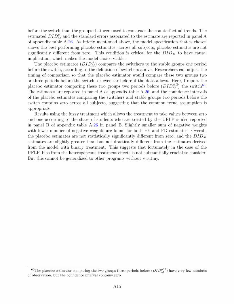
before the switch than the groups that were used to construct the counterfactual trends. Theestimated DIDpl

M and the standard errors associated to the estimate are reported in panel Aof appendix table A.26. As briefly mentioned above, the model specification that is chosenshows the best performing placebo estimates: across all subjects, placebo estimates are notsignificantly different from zero. This condition is critical for the DIDM to have causalimplication, which makes the model choice viable.

The placebo estimator (DIDplM) compares the switchers to the stable groups one period

before the switch, according to the definition of switchers above. Researchers can adjust thetiming of comparison so that the placebo estimator would compare these two groups twoor three periods before the switch, or even far before if the data allows. Here, I report theplacebo estimator comparing these two groups two periods before (DIDpl,2

M ) the switch65.The estimates are reported in panel A of appendix table A.26, and the confidence intervalsof the placebo estimates comparing the switchers and stable groups two periods before theswitch contains zero across all subjects, suggesting that the common trend assumption isappropriate.

Results using the fuzzy treatment which allows the treatment to take values between zeroand one according to the share of students who are treated by the UFLP is also reportedin panel B of appendix table A.26 in panel B. Slightly smaller sum of negative weightswith fewer number of negative weights are found for both FE and FD estimates. Overall,the placebo estimates are not statistically significantly different from zero, and the DIDM

estimates are slightly greater than but not drastically different from the estimates derivedfrom the model with binary treatment. This suggests that fortunately in the case of theUFLP, bias from the heterogeneous treatment effects is not substantially crucial to consider.But this cannot be generalized to other programs without scrutiny.

65The placebo estimator comparing the two groups three periods before (DIDpl,3M ) have very few numbers

of observation, but the confidence interval contains zero.

A15

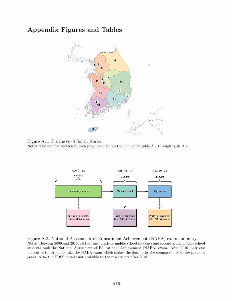
Appendix Figures and Tables

Figure A.1. Provinces of South KoreaNotes: The number written in each province matches the number in table A.1 through table A.4

Figure A.2. National Assessment of Educational Achievement (NAEA) exam summary.Notes: Between 2009 and 2016, all the third grade of middle school students and second grade of high schoolstudents took the National Assessment of Educational Achievement (NAEA) exam. After 2016, only onepercent of the students take the NAEA exam which makes the data lacks the comparability to the previousyears. Also, the EDSS data is not available to the researchers after 2016.

A16

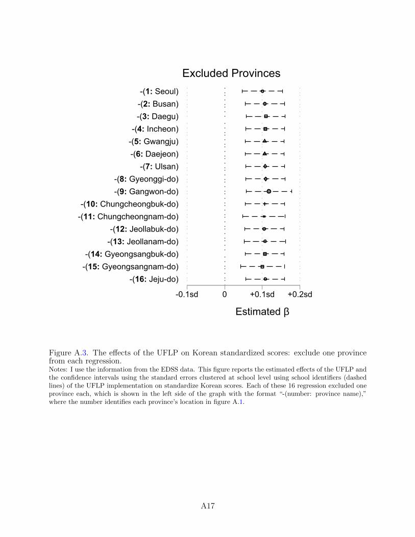
-(1: Seoul)-(2: Busan)-(3: Daegu)

-(4: Incheon)-(5: Gwangju)-(6: Daejeon)

-(7: Ulsan)-(8: Gyeonggi-do)-(9: Gangwon-do)

-(10: Chungcheongbuk-do)-(11: Chungcheongnam-do)

-(12: Jeollabuk-do)-(13: Jeollanam-do)

-(14: Gyeongsangbuk-do)-(15: Gyeongsangnam-do)

-(16: Jeju-do)

-0.1sd 0 +0.1sd +0.2sd

Estimated β

Excluded Provinces

Figure A.3. The effects of the UFLP on Korean standardized scores: exclude one provincefrom each regression.Notes: I use the information from the EDSS data. This figure reports the estimated effects of the UFLP andthe confidence intervals using the standard errors clustered at school level using school identifiers (dashedlines) of the UFLP implementation on standardize Korean scores. Each of these 16 regression excluded oneprovince each, which is shown in the left side of the graph with the format “-(number: province name),”where the number identifies each province’s location in figure A.1.

A17

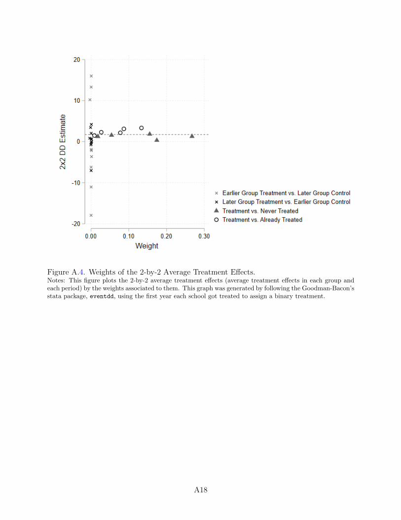
Figure A.4. Weights of the 2-by-2 Average Treatment Effects.Notes: This figure plots the 2-by-2 average treatment effects (average treatment effects in each group andeach period) by the weights associated to them. This graph was generated by following the Goodman-Bacon’sstata package, eventdd, using the first year each school got treated to assign a binary treatment.

A18

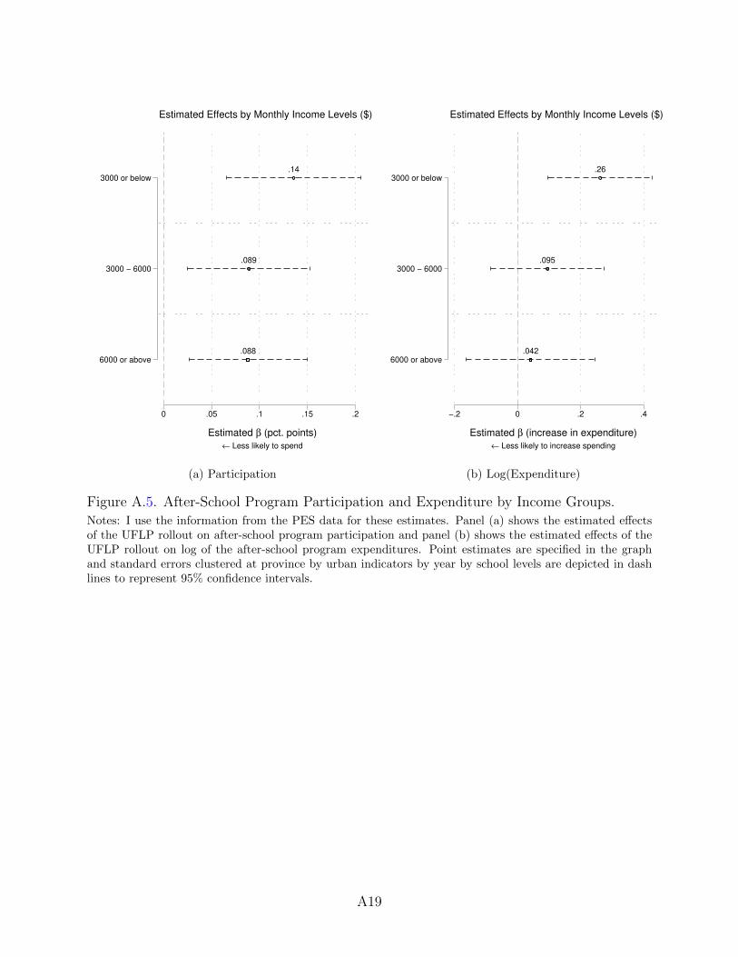
.14

.089

.088

3000 or below

3000 − 6000

6000 or above

0 .05 .1 .15 .2

Estimated β (pct. points)← Less likely to spend

Estimated Effects by Monthly Income Levels ($)

(a) Participation

.26

.095

.042

3000 or below

3000 − 6000

6000 or above

−.2 0 .2 .4

Estimated β (increase in expenditure)← Less likely to increase spending

Estimated Effects by Monthly Income Levels ($)

(b) Log(Expenditure)

Figure A.5. After-School Program Participation and Expenditure by Income Groups.Notes: I use the information from the PES data for these estimates. Panel (a) shows the estimated effectsof the UFLP rollout on after-school program participation and panel (b) shows the estimated effects of theUFLP rollout on log of the after-school program expenditures. Point estimates are specified in the graphand standard errors clustered at province by urban indicators by year by school levels are depicted in dashlines to represent 95% confidence intervals.

A19

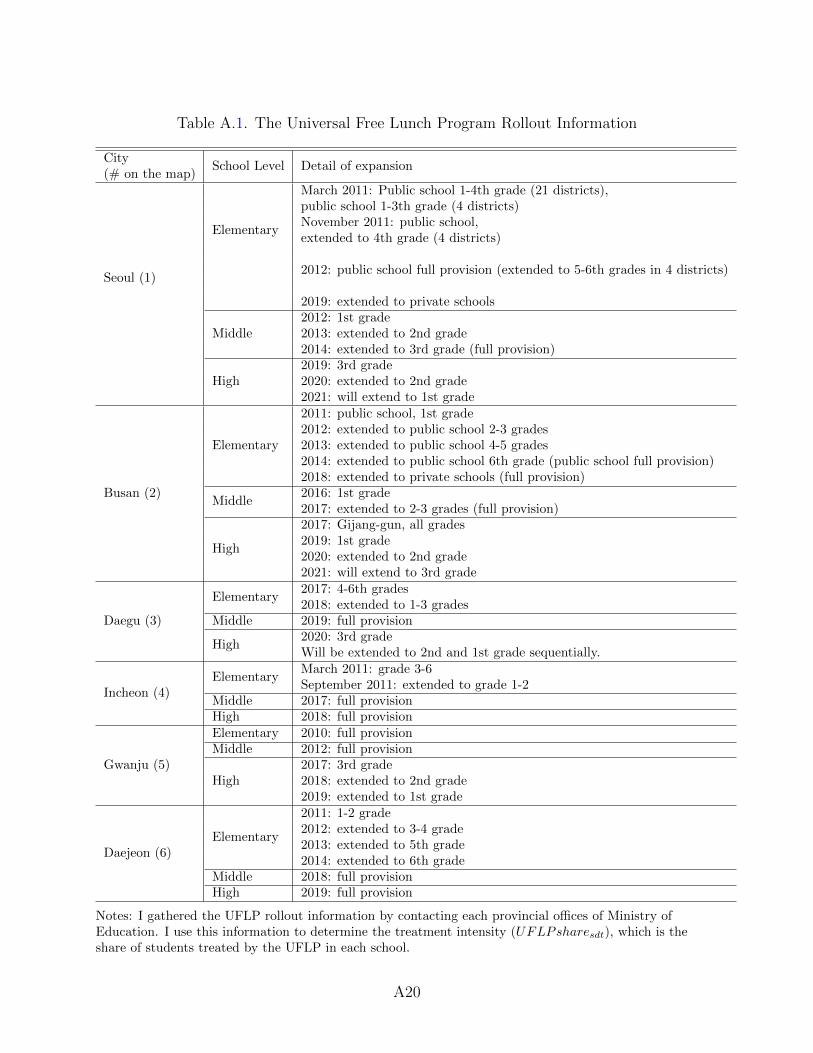
Table A.1. The Universal Free Lunch Program Rollout Information

CitySchool Level Detail of expansion

(# on the map)

Seoul (1)

Elementary

March 2011: Public school 1-4th grade (21 districts),public school 1-3th grade (4 districts)November 2011: public school,extended to 4th grade (4 districts)

2012: public school full provision (extended to 5-6th grades in 4 districts)

2019: extended to private schools

Middle2012: 1st grade2013: extended to 2nd grade2014: extended to 3rd grade (full provision)

High2019: 3rd grade2020: extended to 2nd grade2021: will extend to 1st grade

Busan (2)

Elementary

2011: public school, 1st grade2012: extended to public school 2-3 grades2013: extended to public school 4-5 grades2014: extended to public school 6th grade (public school full provision)2018: extended to private schools (full provision)

Middle2016: 1st grade2017: extended to 2-3 grades (full provision)

High

2017: Gijang-gun, all grades2019: 1st grade2020: extended to 2nd grade2021: will extend to 3rd grade

Daegu (3)

Elementary2017: 4-6th grades2018: extended to 1-3 grades

Middle 2019: full provision

High2020: 3rd gradeWill be extended to 2nd and 1st grade sequentially.

Incheon (4)Elementary

March 2011: grade 3-6September 2011: extended to grade 1-2

Middle 2017: full provisionHigh 2018: full provision

Gwanju (5)

Elementary 2010: full provisionMiddle 2012: full provision

High2017: 3rd grade2018: extended to 2nd grade2019: extended to 1st grade

Daejeon (6)Elementary

2011: 1-2 grade2012: extended to 3-4 grade2013: extended to 5th grade2014: extended to 6th grade

Middle 2018: full provisionHigh 2019: full provision

Notes: I gathered the UFLP rollout information by contacting each provincial offices of Ministry ofEducation. I use this information to determine the treatment intensity (UFLPsharesdt), which is theshare of students treated by the UFLP in each school.

A20

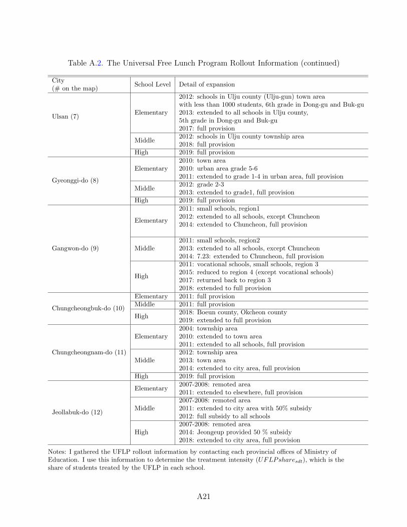
Table A.2. The Universal Free Lunch Program Rollout Information (continued)

CitySchool Level Detail of expansion

(# on the map)

Ulsan (7)

2012: schools in Ulju county (Ulju-gun) town area

Elementarywith less than 1000 students, 6th grade in Dong-gu and Buk-gu2013: extended to all schools in Ulju county,5th grade in Dong-gu and Buk-gu2017: full provision

Middle2012: schools in Ulju county township area2018: full provision

High 2019: full provision

Gyeonggi-do (8)

Elementary2010: town area2010: urban area grade 5-62011: extended to grade 1-4 in urban area, full provision

Middle2012: grade 2-32013: extended to grade1, full provision

High 2019: full provision

Gangwon-do (9)

Elementary

2011: small schools, region12012: extended to all schools, except Chuncheon2014: extended to Chuncheon, full provision

Middle2011: small schools, region22013: extended to all schools, except Chuncheon2014: 7.23: extended to Chuncheon, full provision

High

2011: vocational schools, small schools, region 32015: reduced to region 4 (except vocational schools)2017: returned back to region 32018: extended to full provision

Chungcheongbuk-do (10)

Elementary 2011: full provisionMiddle 2011: full provision

High2018: Boeun county, Okcheon county2019: extended to full provision

Chungcheongnam-do (11)

Elementary2004: township area2010: extended to town area2011: extended to all schools, full provision

Middle2012: township area2013: town area2014: extended to city area, full provision

High 2019: full provision

Jeollabuk-do (12)

Elementary2007-2008: remoted area2011: extended to elsewhere, full provision

Middle2007-2008: remoted area2011: extended to city area with 50% subsidy2012: full subsidy to all schools

High2007-2008: remoted area2014: Jeongeup provided 50 % subsidy2018: extended to city area, full provision

Notes: I gathered the UFLP rollout information by contacting each provincial offices of Ministry ofEducation. I use this information to determine the treatment intensity (UFLPsharesdt), which is theshare of students treated by the UFLP in each school.

A21

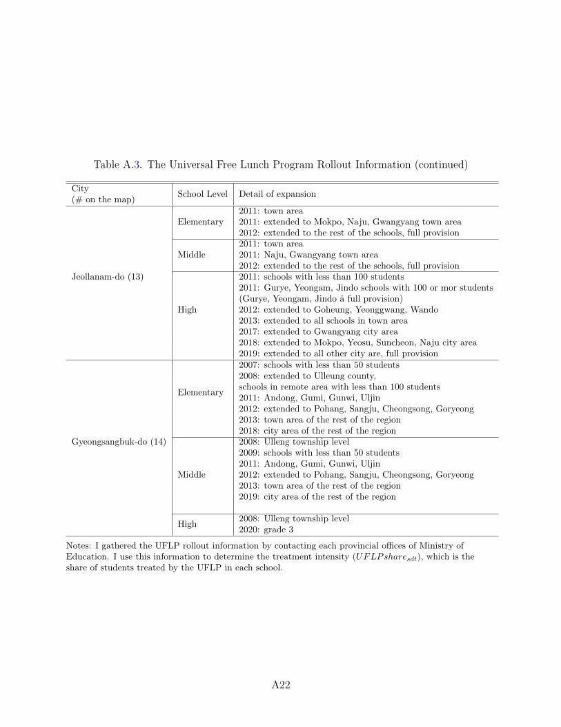
Table A.3. The Universal Free Lunch Program Rollout Information (continued)

CitySchool Level Detail of expansion

(# on the map)

Jeollanam-do (13)

Elementary2011: town area2011: extended to Mokpo, Naju, Gwangyang town area2012: extended to the rest of the schools, full provision

Middle2011: town area2011: Naju, Gwangyang town area2012: extended to the rest of the schools, full provision

High

2011: schools with less than 100 students2011: Gurye, Yeongam, Jindo schools with 100 or mor students(Gurye, Yeongam, Jindo a full provision)2012: extended to Goheung, Yeonggwang, Wando2013: extended to all schools in town area2017: extended to Gwangyang city area2018: extended to Mokpo, Yeosu, Suncheon, Naju city area2019: extended to all other city are, full provision

Gyeongsangbuk-do (14)

Elementary

2007: schools with less than 50 students2008: extended to Ulleung county,schools in remote area with less than 100 students2011: Andong, Gumi, Gunwi, Uljin2012: extended to Pohang, Sangju, Cheongsong, Goryeong2013: town area of the rest of the region2018: city area of the rest of the region

Middle

2008: Ulleng township level2009: schools with less than 50 students2011: Andong, Gumi, Gunwi, Uljin2012: extended to Pohang, Sangju, Cheongsong, Goryeong2013: town area of the rest of the region2019: city area of the rest of the region

High2008: Ulleng township level2020: grade 3

Notes: I gathered the UFLP rollout information by contacting each provincial offices of Ministry ofEducation. I use this information to determine the treatment intensity (UFLPsharesdt), which is theshare of students treated by the UFLP in each school.

A22

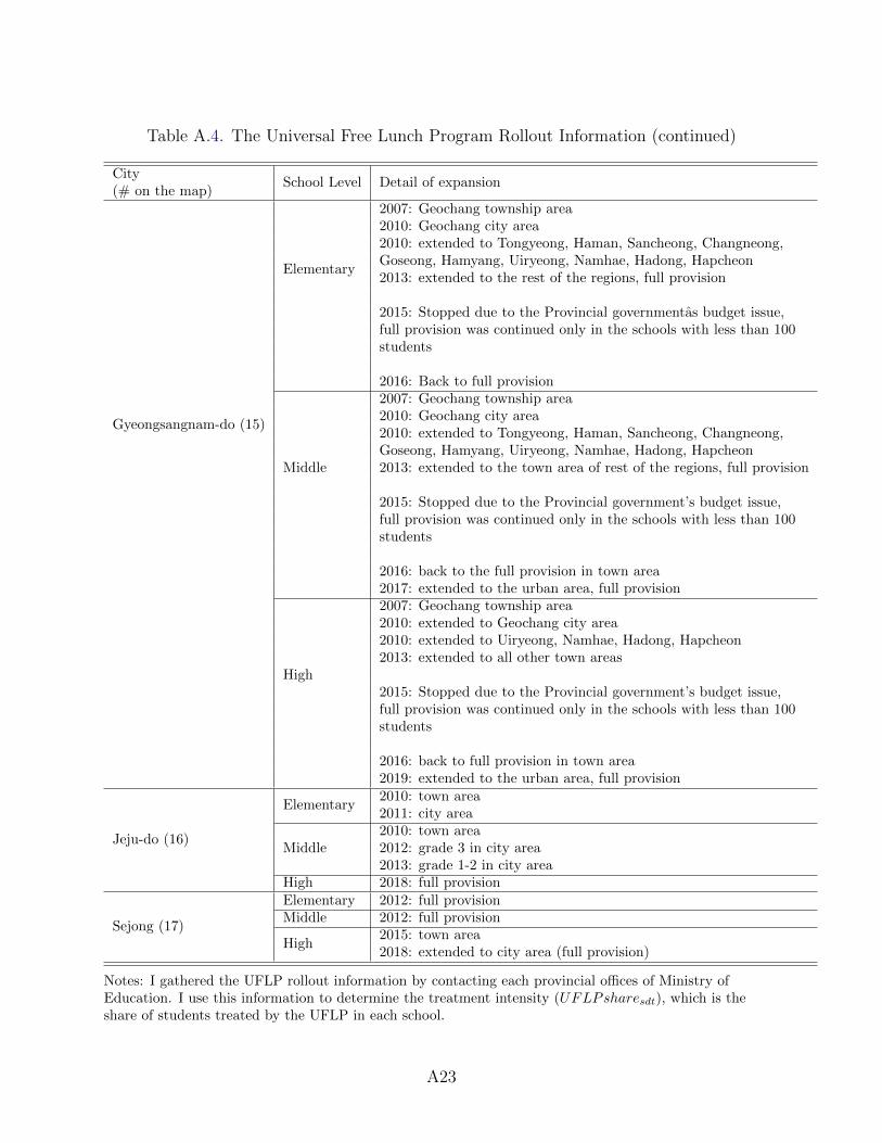
Table A.4. The Universal Free Lunch Program Rollout Information (continued)

CitySchool Level Detail of expansion

(# on the map)

Gyeongsangnam-do (15)

Elementary

2007: Geochang township area2010: Geochang city area2010: extended to Tongyeong, Haman, Sancheong, Changneong,Goseong, Hamyang, Uiryeong, Namhae, Hadong, Hapcheon2013: extended to the rest of the regions, full provision

2015: Stopped due to the Provincial governmentas budget issue,full provision was continued only in the schools with less than 100students

2016: Back to full provision

Middle

2007: Geochang township area2010: Geochang city area2010: extended to Tongyeong, Haman, Sancheong, Changneong,Goseong, Hamyang, Uiryeong, Namhae, Hadong, Hapcheon2013: extended to the town area of rest of the regions, full provision

2015: Stopped due to the Provincial government’s budget issue,full provision was continued only in the schools with less than 100students

2016: back to the full provision in town area2017: extended to the urban area, full provision

High

2007: Geochang township area2010: extended to Geochang city area2010: extended to Uiryeong, Namhae, Hadong, Hapcheon2013: extended to all other town areas

2015: Stopped due to the Provincial government’s budget issue,full provision was continued only in the schools with less than 100students

2016: back to full provision in town area2019: extended to the urban area, full provision

Jeju-do (16)

Elementary2010: town area2011: city area

Middle2010: town area2012: grade 3 in city area2013: grade 1-2 in city area

High 2018: full provision

Sejong (17)

Elementary 2012: full provisionMiddle 2012: full provision

High2015: town area2018: extended to city area (full provision)

Notes: I gathered the UFLP rollout information by contacting each provincial offices of Ministry ofEducation. I use this information to determine the treatment intensity (UFLPsharesdt), which is theshare of students treated by the UFLP in each school.

A23

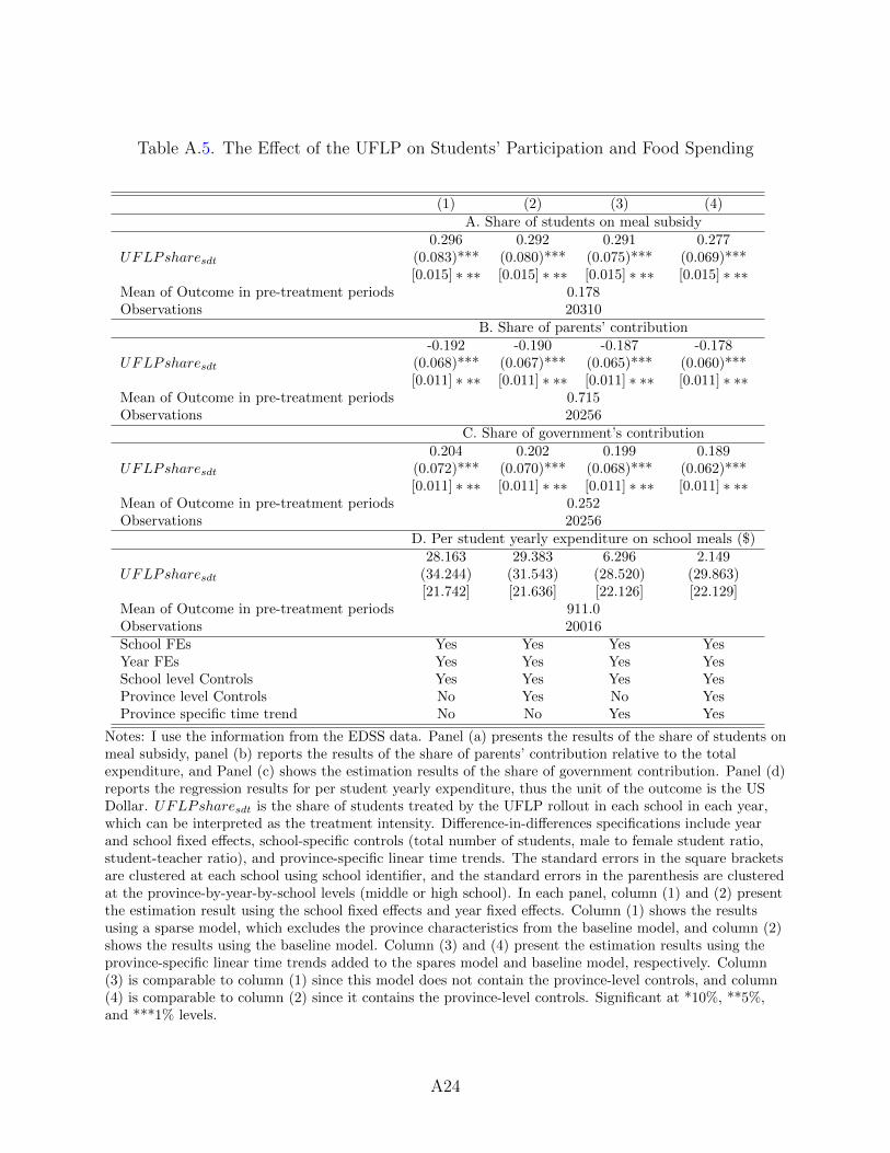
Table A.5. The Effect of the UFLP on Students’ Participation and Food Spending

(1) (2) (3) (4)

A. Share of students on meal subsidy

UFLPsharesdt

0.296(0.083)***[0.015] ∗ ∗∗

0.292(0.080)***[0.015] ∗ ∗∗

0.291(0.075)***[0.015] ∗ ∗∗

0.277(0.069)***[0.015] ∗ ∗∗

Mean of Outcome in pre-treatment periods 0.178Observations 20310

B. Share of parents’ contribution

UFLPsharesdt

-0.192(0.068)***[0.011] ∗ ∗∗

-0.190(0.067)***[0.011] ∗ ∗∗

-0.187(0.065)***[0.011] ∗ ∗∗

-0.178(0.060)***[0.011] ∗ ∗∗

Mean of Outcome in pre-treatment periods 0.715Observations 20256

C. Share of government’s contribution

UFLPsharesdt

0.204(0.072)***[0.011] ∗ ∗∗

0.202(0.070)***[0.011] ∗ ∗∗

0.199(0.068)***[0.011] ∗ ∗∗

0.189(0.062)***[0.011] ∗ ∗∗

Mean of Outcome in pre-treatment periods 0.252Observations 20256

D. Per student yearly expenditure on school meals ($)

UFLPsharesdt

28.163(34.244)[21.742]

29.383(31.543)[21.636]

6.296(28.520)[22.126]

2.149(29.863)[22.129]

Mean of Outcome in pre-treatment periods 911.0Observations 20016School FEs Yes Yes Yes YesYear FEs Yes Yes Yes YesSchool level Controls Yes Yes Yes YesProvince level Controls No Yes No YesProvince specific time trend No No Yes Yes

Notes: I use the information from the EDSS data. Panel (a) presents the results of the share of students onmeal subsidy, panel (b) reports the results of the share of parents’ contribution relative to the totalexpenditure, and Panel (c) shows the estimation results of the share of government contribution. Panel (d)reports the regression results for per student yearly expenditure, thus the unit of the outcome is the USDollar. UFLPsharesdt is the share of students treated by the UFLP rollout in each school in each year,which can be interpreted as the treatment intensity. Difference-in-differences specifications include yearand school fixed effects, school-specific controls (total number of students, male to female student ratio,student-teacher ratio), and province-specific linear time trends. The standard errors in the square bracketsare clustered at each school using school identifier, and the standard errors in the parenthesis are clusteredat the province-by-year-by-school levels (middle or high school). In each panel, column (1) and (2) presentthe estimation result using the school fixed effects and year fixed effects. Column (1) shows the resultsusing a sparse model, which excludes the province characteristics from the baseline model, and column (2)shows the results using the baseline model. Column (3) and (4) present the estimation results using theprovince-specific linear time trends added to the spares model and baseline model, respectively. Column(3) is comparable to column (1) since this model does not contain the province-level controls, and column(4) is comparable to column (2) since it contains the province-level controls. Significant at *10%, **5%,and ***1% levels.

A24

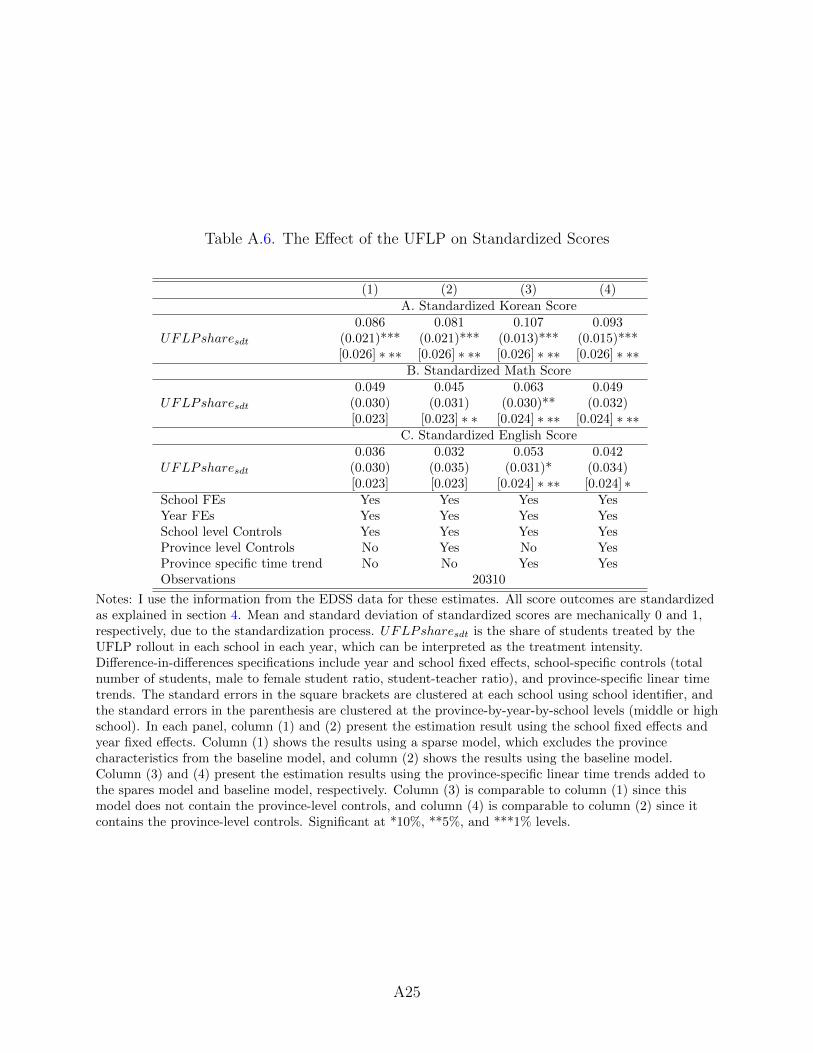
Table A.6. The Effect of the UFLP on Standardized Scores

(1) (2) (3) (4)

A. Standardized Korean Score

UFLPsharesdt

0.086(0.021)***[0.026] ∗ ∗∗

0.081(0.021)***[0.026] ∗ ∗∗

0.107(0.013)***[0.026] ∗ ∗∗

0.093(0.015)***[0.026] ∗ ∗∗

B. Standardized Math Score

UFLPsharesdt

0.049(0.030)[0.023]

0.045(0.031)

[0.023] ∗ ∗

0.063(0.030)**

[0.024] ∗ ∗∗

0.049(0.032)

[0.024] ∗ ∗∗C. Standardized English Score

UFLPsharesdt

0.036(0.030)[0.023]

0.032(0.035)[0.023]

0.053(0.031)*

[0.024] ∗ ∗∗

0.042(0.034)[0.024] ∗

School FEs Yes Yes Yes YesYear FEs Yes Yes Yes YesSchool level Controls Yes Yes Yes YesProvince level Controls No Yes No YesProvince specific time trend No No Yes YesObservations 20310

Notes: I use the information from the EDSS data for these estimates. All score outcomes are standardizedas explained in section 4. Mean and standard deviation of standardized scores are mechanically 0 and 1,respectively, due to the standardization process. UFLPsharesdt is the share of students treated by theUFLP rollout in each school in each year, which can be interpreted as the treatment intensity.Difference-in-differences specifications include year and school fixed effects, school-specific controls (totalnumber of students, male to female student ratio, student-teacher ratio), and province-specific linear timetrends. The standard errors in the square brackets are clustered at each school using school identifier, andthe standard errors in the parenthesis are clustered at the province-by-year-by-school levels (middle or highschool). In each panel, column (1) and (2) present the estimation result using the school fixed effects andyear fixed effects. Column (1) shows the results using a sparse model, which excludes the provincecharacteristics from the baseline model, and column (2) shows the results using the baseline model.Column (3) and (4) present the estimation results using the province-specific linear time trends added tothe spares model and baseline model, respectively. Column (3) is comparable to column (1) since thismodel does not contain the province-level controls, and column (4) is comparable to column (2) since itcontains the province-level controls. Significant at *10%, **5%, and ***1% levels.

A25

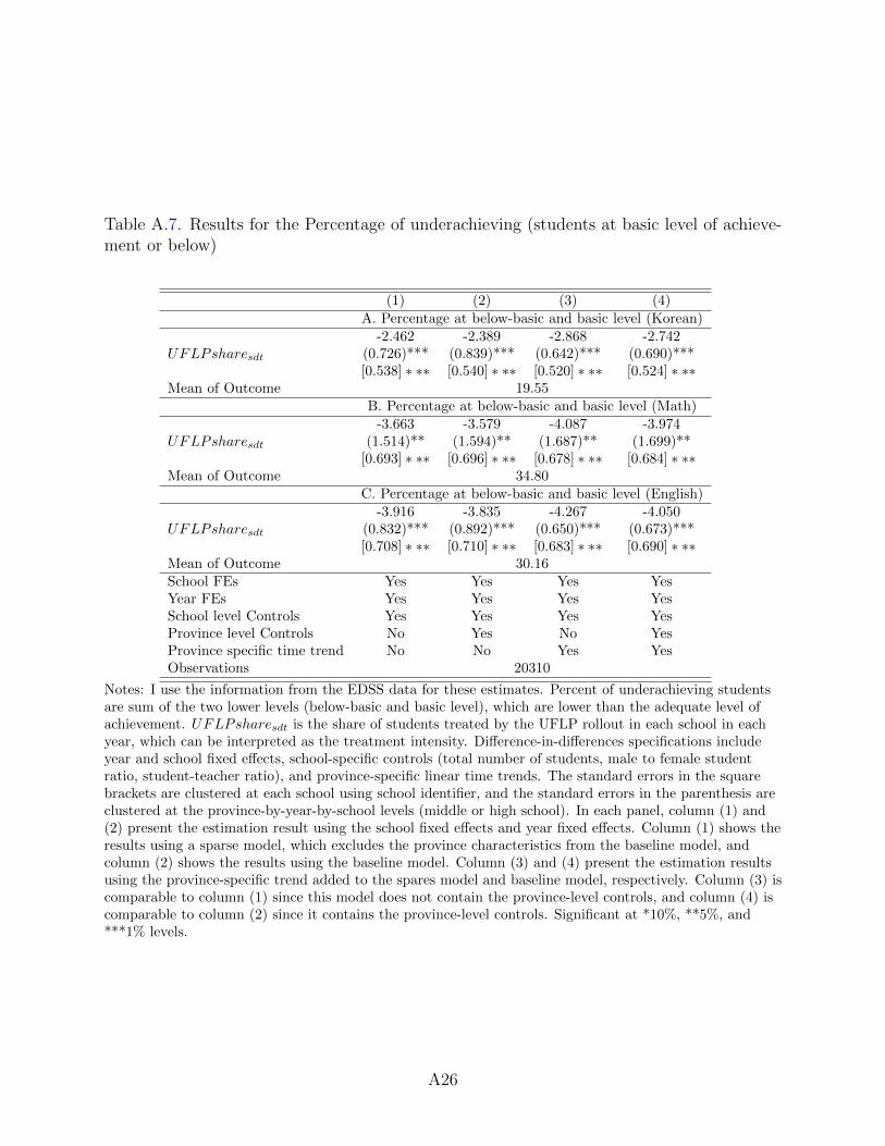
Table A.7. Results for the Percentage of underachieving (students at basic level of achieve-ment or below)

(1) (2) (3) (4)

A. Percentage at below-basic and basic level (Korean)

UFLPsharesdt

-2.462(0.726)***[0.538] ∗ ∗∗

-2.389(0.839)***[0.540] ∗ ∗∗

-2.868(0.642)***[0.520] ∗ ∗∗

-2.742(0.690)***[0.524] ∗ ∗∗

Mean of Outcome 19.55B. Percentage at below-basic and basic level (Math)

UFLPsharesdt

-3.663(1.514)**

[0.693] ∗ ∗∗

-3.579(1.594)**

[0.696] ∗ ∗∗

-4.087(1.687)**

[0.678] ∗ ∗∗

-3.974(1.699)**

[0.684] ∗ ∗∗Mean of Outcome 34.80

C. Percentage at below-basic and basic level (English)

UFLPsharesdt

-3.916(0.832)***[0.708] ∗ ∗∗

-3.835(0.892)***[0.710] ∗ ∗∗

-4.267(0.650)***[0.683] ∗ ∗∗

-4.050(0.673)***[0.690] ∗ ∗∗

Mean of Outcome 30.16School FEs Yes Yes Yes YesYear FEs Yes Yes Yes YesSchool level Controls Yes Yes Yes YesProvince level Controls No Yes No YesProvince specific time trend No No Yes YesObservations 20310

Notes: I use the information from the EDSS data for these estimates. Percent of underachieving studentsare sum of the two lower levels (below-basic and basic level), which are lower than the adequate level ofachievement. UFLPsharesdt is the share of students treated by the UFLP rollout in each school in eachyear, which can be interpreted as the treatment intensity. Difference-in-differences specifications includeyear and school fixed effects, school-specific controls (total number of students, male to female studentratio, student-teacher ratio), and province-specific linear time trends. The standard errors in the squarebrackets are clustered at each school using school identifier, and the standard errors in the parenthesis areclustered at the province-by-year-by-school levels (middle or high school). In each panel, column (1) and(2) present the estimation result using the school fixed effects and year fixed effects. Column (1) shows theresults using a sparse model, which excludes the province characteristics from the baseline model, andcolumn (2) shows the results using the baseline model. Column (3) and (4) present the estimation resultsusing the province-specific trend added to the spares model and baseline model, respectively. Column (3) iscomparable to column (1) since this model does not contain the province-level controls, and column (4) iscomparable to column (2) since it contains the province-level controls. Significant at *10%, **5%, and***1% levels.

A26

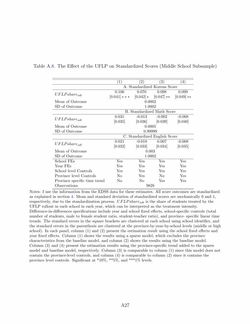
Table A.8. The Effect of the UFLP on Standardized Scores (Middle School Subsample)

(1) (2) (3) (4)

A. Standardized Korean Score

UFLPsharesdt0.106

[0.041] ∗ ∗ ∗0.070

[0.042] ∗0.098

[0.047] ∗∗0.099

[0.049] ∗∗Mean of Outcome 0.0002SD of Outcome 1.0002

B. Standardized Math Score

UFLPsharesdt0.031[0.035]

-0.013[0.036]

-0.002[0.039]

-0.008[0.040]

Mean of Outcome 0.0005SD of Outcome 0.99999

C. Standardized English Score

UFLPsharesdt0.021[0.032]

-0.018[0.033]

0.007[0.034]

-0.008[0.035]

Mean of Outcome 0.003SD of Outcome 1.0002School FEs Yes Yes Yes YesYear FEs Yes Yes Yes YesSchool level Controls Yes Yes Yes YesProvince level Controls No Yes No YesProvince specific time trend No No Yes YesObservations 9828

Notes: I use the information from the EDSS data for these estimates. All score outcomes are standardizedas explained in section 4. Mean and standard deviation of standardized scores are mechanically 0 and 1,respectively, due to the standardization process. UFLPsharesdt is the share of students treated by theUFLP rollout in each school in each year, which can be interpreted as the treatment intensity.Difference-in-differences specifications include year and school fixed effects, school-specific controls (totalnumber of students, male to female student ratio, student-teacher ratio), and province- specific linear timetrends. The standard errors in the square brackets are clustered at each school using school identifier, andthe standard errors in the parenthesis are clustered at the province-by-year-by-school levels (middle or highschool). In each panel, column (1) and (2) present the estimation result using the school fixed effects andyear fixed effects. Column (1) shows the results using a sparse model, which excludes the provincecharacteristics from the baseline model, and column (2) shows the results using the baseline model.Column (3) and (4) present the estimation results using the province-specific trend added to the sparesmodel and baseline model, respectively. Column (3) is comparable to column (1) since this model does notcontain the province-level controls, and column (4) is comparable to column (2) since it contains theprovince level controls. Significant at *10%, **5%, and ***1% levels.

A27

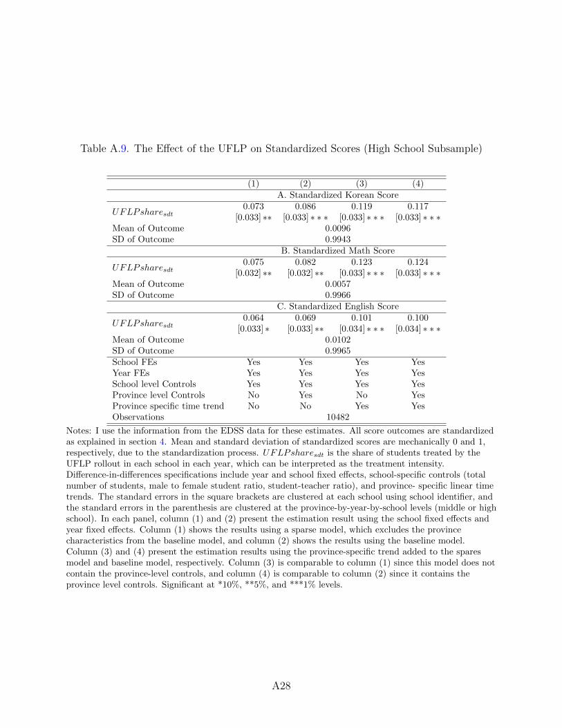
Table A.9. The Effect of the UFLP on Standardized Scores (High School Subsample)

(1) (2) (3) (4)

A. Standardized Korean Score

UFLPsharesdt0.073

[0.033] ∗∗0.086

[0.033] ∗ ∗ ∗0.119

[0.033] ∗ ∗ ∗0.117

[0.033] ∗ ∗ ∗Mean of Outcome 0.0096SD of Outcome 0.9943

B. Standardized Math Score

UFLPsharesdt0.075

[0.032] ∗∗0.082

[0.032] ∗∗0.123

[0.033] ∗ ∗ ∗0.124

[0.033] ∗ ∗ ∗Mean of Outcome 0.0057SD of Outcome 0.9966

C. Standardized English Score

UFLPsharesdt0.064

[0.033] ∗0.069

[0.033] ∗∗0.101

[0.034] ∗ ∗ ∗0.100

[0.034] ∗ ∗ ∗Mean of Outcome 0.0102SD of Outcome 0.9965School FEs Yes Yes Yes YesYear FEs Yes Yes Yes YesSchool level Controls Yes Yes Yes YesProvince level Controls No Yes No YesProvince specific time trend No No Yes YesObservations 10482

Notes: I use the information from the EDSS data for these estimates. All score outcomes are standardizedas explained in section 4. Mean and standard deviation of standardized scores are mechanically 0 and 1,respectively, due to the standardization process. UFLPsharesdt is the share of students treated by theUFLP rollout in each school in each year, which can be interpreted as the treatment intensity.Difference-in-differences specifications include year and school fixed effects, school-specific controls (totalnumber of students, male to female student ratio, student-teacher ratio), and province- specific linear timetrends. The standard errors in the square brackets are clustered at each school using school identifier, andthe standard errors in the parenthesis are clustered at the province-by-year-by-school levels (middle or highschool). In each panel, column (1) and (2) present the estimation result using the school fixed effects andyear fixed effects. Column (1) shows the results using a sparse model, which excludes the provincecharacteristics from the baseline model, and column (2) shows the results using the baseline model.Column (3) and (4) present the estimation results using the province-specific trend added to the sparesmodel and baseline model, respectively. Column (3) is comparable to column (1) since this model does notcontain the province-level controls, and column (4) is comparable to column (2) since it contains theprovince level controls. Significant at *10%, **5%, and ***1% levels.

A28

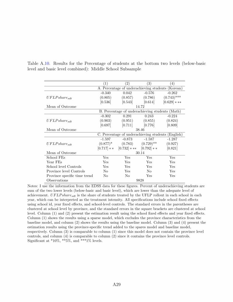
Table A.10. Results for the Percentage of students at the bottom two levels (below-basiclevel and basic level combined): Middle School Subsample

(1) (2) (3) (4)

A. Percentage of underachieving students (Korean)

UFLPsharesdt

-0.340(0.805)[0.536]

0.042(0.857)[0.543]

-0.576(0.786)[0.614]

-0.262(0.743)***[0.629] ∗ ∗∗

Mean of Outcome 14.72B. Percentage of underachieving students (Math)

UFLPsharesdt

-0.302(0.903)[0.697]

0.291(0.951)[0.711]

0.243(0.855)[0.776]

-0.224(0.824)[0.809]

Mean of Outcome 38.46C. Percentage of underachieving students (English)

UFLPsharesdt

-1.597(0.877)*

[0.717] ∗ ∗

-0.873(0.783)

[0.732] ∗ ∗∗

-1.587(0.729)**[0.792] ∗ ∗

-1.287(0.927)[0.821]

Mean of Outcome 30.14School FEs Yes Yes Yes YesYear FEs Yes Yes Yes YesSchool level Controls Yes Yes Yes YesProvince level Controls No Yes No YesProvince specific time trend No No Yes YesObservations 9828

Notes: I use the information from the EDSS data for these figures. Percent of underachieving students aresum of the two lower levels (below-basic and basic level), which are lower than the adequate level ofachievement. UFLPsharesdt is the share of students treated by the UFLP rollout in each school in eachyear, which can be interpreted as the treatment intensity. All specifications include school fixed effectsusing school id, year fixed effects, and school-level controls. The standard errors in the parentheses areclustered at school level by province, and the standard errors in the square brackets are clustered at schoollevel. Column (1) and (2) present the estimation result using the school fixed effects and year fixed effects.Column (1) shows the results using a sparse model, which excludes the province characteristics from thebaseline model, and column (2) shows the results using the baseline model. Column (3) and (4) present theestimation results using the province-specific trend added to the spares model and baseline model,respectively. Column (3) is comparable to column (1) since this model does not contain the province levelcontrols, and column (4) is comparable to column (2) since it contains the province level controls.Significant at *10%, **5%, and ***1% levels.

A29

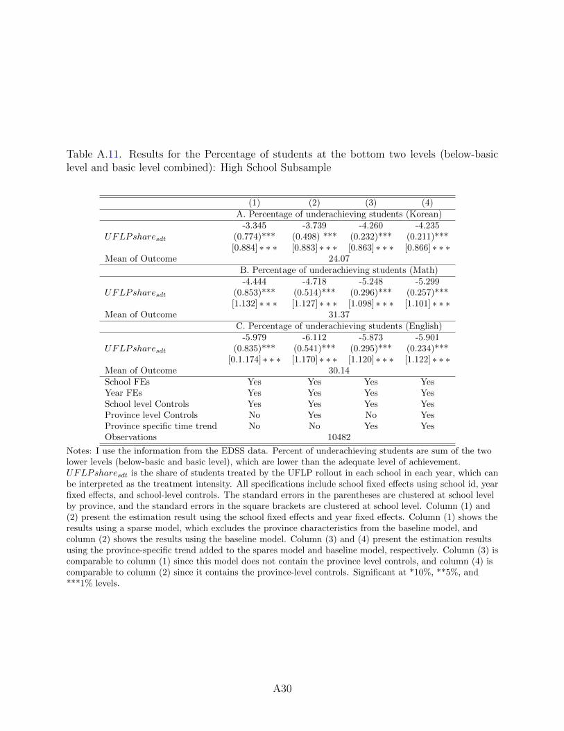
Table A.11. Results for the Percentage of students at the bottom two levels (below-basiclevel and basic level combined): High School Subsample

(1) (2) (3) (4)

A. Percentage of underachieving students (Korean)

UFLPsharesdt

-3.345(0.774)***[0.884] ∗ ∗ ∗

-3.739(0.498) ***[0.883] ∗ ∗ ∗

-4.260(0.232)***[0.863] ∗ ∗ ∗

-4.235(0.211)***[0.866] ∗ ∗ ∗

Mean of Outcome 24.07B. Percentage of underachieving students (Math)

UFLPsharesdt

-4.444(0.853)***[1.132] ∗ ∗ ∗

-4.718(0.514)***[1.127] ∗ ∗ ∗

-5.248(0.296)***[1.098] ∗ ∗ ∗

-5.299(0.257)***[1.101] ∗ ∗ ∗

Mean of Outcome 31.37C. Percentage of underachieving students (English)

UFLPsharesdt

-5.979(0.835)***

[0.1.174] ∗ ∗ ∗

-6.112(0.541)***[1.170] ∗ ∗ ∗

-5.873(0.295)***[1.120] ∗ ∗ ∗

-5.901(0.234)***[1.122] ∗ ∗ ∗

Mean of Outcome 30.14School FEs Yes Yes Yes YesYear FEs Yes Yes Yes YesSchool level Controls Yes Yes Yes YesProvince level Controls No Yes No YesProvince specific time trend No No Yes YesObservations 10482

Notes: I use the information from the EDSS data. Percent of underachieving students are sum of the twolower levels (below-basic and basic level), which are lower than the adequate level of achievement.UFLPsharesdt is the share of students treated by the UFLP rollout in each school in each year, which canbe interpreted as the treatment intensity. All specifications include school fixed effects using school id, yearfixed effects, and school-level controls. The standard errors in the parentheses are clustered at school levelby province, and the standard errors in the square brackets are clustered at school level. Column (1) and(2) present the estimation result using the school fixed effects and year fixed effects. Column (1) shows theresults using a sparse model, which excludes the province characteristics from the baseline model, andcolumn (2) shows the results using the baseline model. Column (3) and (4) present the estimation resultsusing the province-specific trend added to the spares model and baseline model, respectively. Column (3) iscomparable to column (1) since this model does not contain the province level controls, and column (4) iscomparable to column (2) since it contains the province-level controls. Significant at *10%, **5%, and***1% levels.

A30

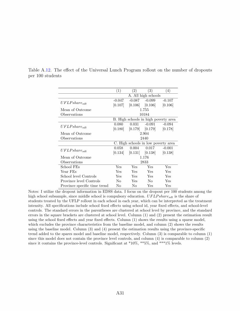
Table A.12. The effect of the Universal Lunch Program rollout on the number of dropoutsper 100 students

(1) (2) (3) (4)

A. All high schools

UFLPsharesdt-0.047[0.107]

-0.087[0.106]

-0.099[0.106]

-0.107[0.106]

Mean of Outcome 1.755Observations 10184

B. High schools in high poverty area

UFLPsharesdt0.080[0.180]

0.031[0.179]

-0.091[0.179]

-0.094[0.178]

Mean of Outcome 2.904Observations 2440

C. High schools in low poverty area

UFLPsharesdt0.058[0.134]

0.004[0.131]

0.017[0.138]

-0.001[0.138]

Mean of Outcome 1.176Observations 2833School FEs Yes Yes Yes YesYear FEs Yes Yes Yes YesSchool level Controls Yes Yes Yes YesProvince level Controls No Yes No YesProvince specific time trend No No Yes Yes

Notes: I utilize the dropout information in EDSS data. I focus on the dropout per 100 students among thehigh school subsample, since middle school is compulsory education. UFLPsharesdt is the share ofstudents treated by the UFLP rollout in each school in each year, which can be interpreted as the treatmentintensity. All specifications include school fixed effects using school id, year fixed effects, and school-levelcontrols. The standard errors in the parentheses are clustered at school level by province, and the standarderrors in the square brackets are clustered at school level. Column (1) and (2) present the estimation resultusing the school fixed effects and year fixed effects. Column (1) shows the results using a sparse model,which excludes the province characteristics from the baseline model, and column (2) shows the resultsusing the baseline model. Column (3) and (4) present the estimation results using the province-specifictrend added to the spares model and baseline model, respectively. Column (3) is comparable to column (1)since this model does not contain the province level controls, and column (4) is comparable to column (2)since it contains the province-level controls. Significant at *10%, **5%, and ***1% levels.

A31

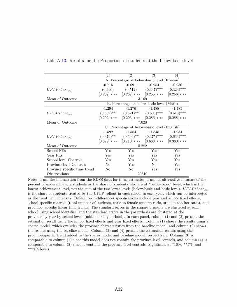
Table A.13. Results for the Proportion of students at the below-basic level

(1) (2) (3) (4)

A. Percentage at below-basic level (Korean)

UFLPsharesdt

-0.715(0.490)

[0.267] ∗ ∗∗

-0.691(0.512)

[0.267] ∗ ∗∗

-0.954(0.337)***[0.255] ∗ ∗∗

-0.936(0.323)***[0.256] ∗ ∗∗

Mean of Outcome 3.169B. Percentage at below-basic level (Math)

UFLPsharesdt

-1.294(0.502)**

[0.292] ∗ ∗∗

-1.276(0.521)**

[0.293] ∗ ∗∗

-1.488(0.505)***[0.286] ∗ ∗∗

-1.485(0.513)***[0.288] ∗ ∗∗

Mean of Outcome 7.028C. Percentage at below-basic level (English)

UFLPsharesdt

-1.592(0.379)**

[0.379] ∗ ∗∗

-1.584(0.609)**

[0.710] ∗ ∗∗

-1.845(0.375)***[0.683] ∗ ∗∗

-1.934(0.633)***[0.380] ∗ ∗∗

Mean of Outcome 5.282School FEs Yes Yes Yes YesYear FEs Yes Yes Yes YesSchool level Controls Yes Yes Yes YesProvince level Controls No Yes No YesProvince specific time trend No No Yes YesObservations 20310

Notes: I use the information from the EDSS data for these estimates. I use an alternative measure of thepercent of underachieving students as the share of students who are at “below-basic” level, which is thelowest achievement level, not the sum of the two lower levels (below-basic and basic level). UFLPsharesdtis the share of students treated by the UFLP rollout in each school in each year, which can be interpretedas the treatment intensity. Difference-in-differences specifications include year and school fixed effects,school-specific controls (total number of students, male to female student ratio, student-teacher ratio), andprovince- specific linear time trends. The standard errors in the square brackets are clustered at eachschool using school identifier, and the standard errors in the parenthesis are clustered at theprovince-by-year-by-school levels (middle or high school). In each panel, column (1) and (2) present theestimation result using the school fixed effects and year fixed effects. Column (1) shows the results using asparse model, which excludes the province characteristics from the baseline model, and column (2) showsthe results using the baseline model. Column (3) and (4) present the estimation results using theprovince-specific trend added to the spares model and baseline model, respectively. Column (3) iscomparable to column (1) since this model does not contain the province-level controls, and column (4) iscomparable to column (2) since it contains the province-level controls. Significant at *10%, **5%, and***1% levels.

A32

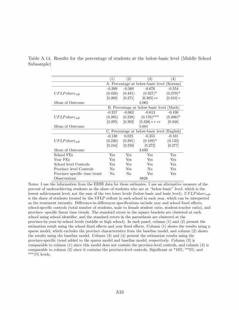
Table A.14. Results for the percentage of students at the below-basic level (Middle SchoolSubsample)

(1) (2) (3) (4)

A. Percentage at below-basic level (Korean)

UFLPsharesdt

-0.399(0.428)[0.268]

-0.360(0.431)[0.271]

-0.676(0.327)*[0.305] ∗∗

-0.554(0.279)*[0.310] ∗

Mean of Outcome 2.065B. Percentage at below-basic level (Math)

UFLPsharesdt

-0.257(0.205)[0.295]

-0.062(0.228)[0.302]

-0.613(0.176)***

[0.338] ∗ ∗ ∗∗

-0.430(0.206)*[0.348]

Mean of Outcome 5.681C. Percentage at below-basic level (English)

UFLPsharesdt

-0.130(0.226)[0.244]

0.025(0.291)[0.250]

-0.355(0.189)*[0.272]

-0.161(0.133)[0.277]

Mean of Outcome 3.695School FEs Yes Yes Yes YesYear FEs Yes Yes Yes YesSchool level Controls Yes Yes Yes YesProvince level Controls No Yes No YesProvince specific time trend No No Yes YesObservations 9828

Notes: I use the information from the EDSS data for these estimates. I use an alternative measure of thepercent of underachieving students as the share of students who are at “below-basic” level, which is thelowest achievement level, not the sum of the two lower levels (below-basic and basic level). UFLPsharesdtis the share of students treated by the UFLP rollout in each school in each year, which can be interpretedas the treatment intensity. Difference-in-differences specifications include year and school fixed effects,school-specific controls (total number of students, male to female student ratio, student-teacher ratio), andprovince- specific linear time trends. The standard errors in the square brackets are clustered at eachschool using school identifier, and the standard errors in the parenthesis are clustered at theprovince-by-year-by-school levels (middle or high school). In each panel, column (1) and (2) present theestimation result using the school fixed effects and year fixed effects. Column (1) shows the results using asparse model, which excludes the province characteristics from the baseline model, and column (2) showsthe results using the baseline model. Column (3) and (4) present the estimation results using theprovince-specific trend added to the spares model and baseline model, respectively. Column (3) iscomparable to column (1) since this model does not contain the province-level controls, and column (4) iscomparable to column (2) since it contains the province-level controls. Significant at *10%, **5%, and***1% levels.

A33

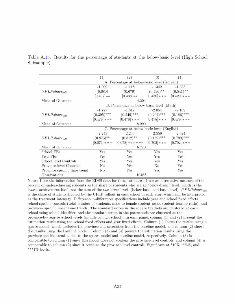
Table A.15. Results for the percentage of students at the below-basic level (High SchoolSubsample)

(1) (2) (3) (4)

A. Percentage at below-basic level (Korean)

UFLPsharesdt

-1.009(0.680)

[0.437] ∗∗

-1.118(0.679)

[0.438] ∗∗

-1.342(0.496)**

[0.430] ∗ ∗ ∗

-1.335(0.541)**

[0.429] ∗ ∗ ∗Mean of Outcome 4.204

B. Percentage at below-basic level (Math)

UFLPsharesdt

-1.727(0.395)***[0.479] ∗ ∗ ∗

-1.817(0.249)***[0.478] ∗ ∗ ∗

-2.054(0.202)***[0.478] ∗ ∗ ∗

-2.109(0.186)***[0.479] ∗ ∗ ∗

Mean of Outcome 8.290C. Percentage at below-basic level (English)

UFLPsharesdt

-2.243(0.873)**

[0.676] ∗ ∗ ∗

-2.243(0.812)**

[0.678] ∗ ∗ ∗ ∗ ∗∗

-2.559(0.189)***[0.702] ∗ ∗ ∗

-2.624(0.799)***[0.702] ∗ ∗ ∗

Mean of Outcome 6.770School FEs Yes Yes Yes YesYear FEs Yes Yes Yes YesSchool level Controls Yes Yes Yes YesProvince level Controls No Yes No YesProvince specific time trend No No Yes YesObservations 10482

Notes: I use the information from the EDSS data for these estimates. I use an alternative measure of thepercent of underachieving students as the share of students who are at “below-basic” level, which is thelowest achievement level, not the sum of the two lower levels (below-basic and basic level). UFLPsharesdtis the share of students treated by the UFLP rollout in each school in each year, which can be interpretedas the treatment intensity. Difference-in-differences specifications include year and school fixed effects,school-specific controls (total number of students, male to female student ratio, student-teacher ratio), andprovince- specific linear time trends. The standard errors in the square brackets are clustered at eachschool using school identifier, and the standard errors in the parenthesis are clustered at theprovince-by-year-by-school levels (middle or high school). In each panel, column (1) and (2) present theestimation result using the school fixed effects and year fixed effects. Column (1) shows the results using asparse model, which excludes the province characteristics from the baseline model, and column (2) showsthe results using the baseline model. Column (3) and (4) present the estimation results using theprovince-specific trend added to the spares model and baseline model, respectively. Column (3) iscomparable to column (1) since this model does not contain the province-level controls, and column (4) iscomparable to column (2) since it contains the province-level controls. Significant at *10%, **5%, and***1% levels.

A34

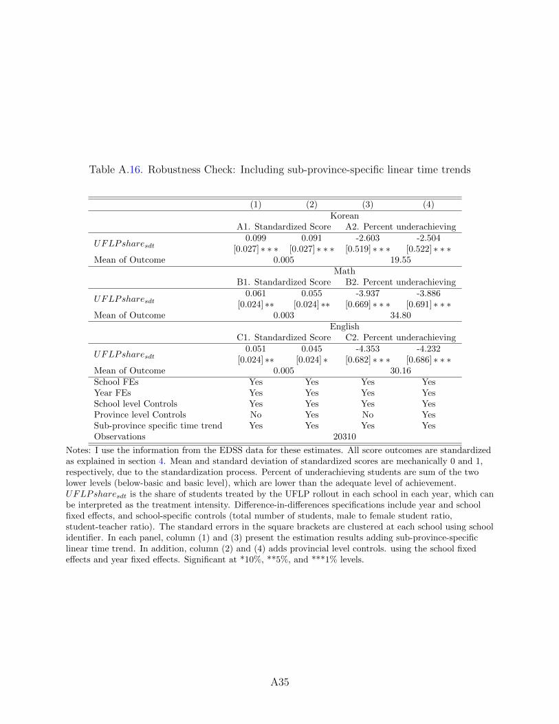
Table A.16. Robustness Check: Including sub-province-specific linear time trends

(1) (2) (3) (4)

KoreanA1. Standardized Score A2. Percent underachieving

UFLPsharesdt0.099

[0.027] ∗ ∗ ∗0.091

[0.027] ∗ ∗ ∗-2.603

[0.519] ∗ ∗ ∗-2.504

[0.522] ∗ ∗ ∗Mean of Outcome 0.005 19.55

MathB1. Standardized Score B2. Percent underachieving

UFLPsharesdt0.061

[0.024] ∗∗0.055

[0.024] ∗∗-3.937

[0.669] ∗ ∗ ∗-3.886

[0.691] ∗ ∗ ∗Mean of Outcome 0.003 34.80

EnglishC1. Standardized Score C2. Percent underachieving

UFLPsharesdt0.051

[0.024] ∗∗0.045

[0.024] ∗-4.353

[0.682] ∗ ∗ ∗-4.232

[0.686] ∗ ∗ ∗Mean of Outcome 0.005 30.16School FEs Yes Yes Yes YesYear FEs Yes Yes Yes YesSchool level Controls Yes Yes Yes YesProvince level Controls No Yes No YesSub-province specific time trend Yes Yes Yes YesObservations 20310

Notes: I use the information from the EDSS data for these estimates. All score outcomes are standardizedas explained in section 4. Mean and standard deviation of standardized scores are mechanically 0 and 1,respectively, due to the standardization process. Percent of underachieving students are sum of the twolower levels (below-basic and basic level), which are lower than the adequate level of achievement.UFLPsharesdt is the share of students treated by the UFLP rollout in each school in each year, which canbe interpreted as the treatment intensity. Difference-in-differences specifications include year and schoolfixed effects, and school-specific controls (total number of students, male to female student ratio,student-teacher ratio). The standard errors in the square brackets are clustered at each school using schoolidentifier. In each panel, column (1) and (3) present the estimation results adding sub-province-specificlinear time trend. In addition, column (2) and (4) adds provincial level controls. using the school fixedeffects and year fixed effects. Significant at *10%, **5%, and ***1% levels.

A35

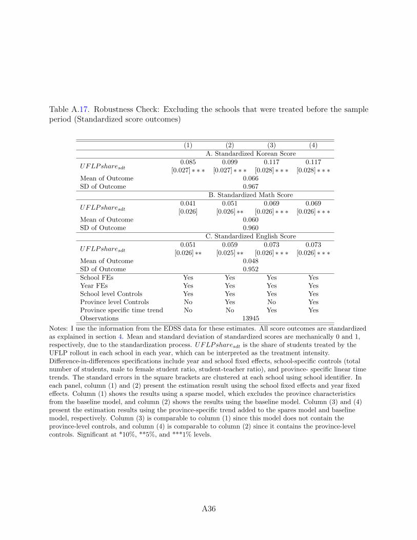
Table A.17. Robustness Check: Excluding the schools that were treated before the sampleperiod (Standardized score outcomes)

(1) (2) (3) (4)

A. Standardized Korean Score

UFLPsharesdt0.085

[0.027] ∗ ∗ ∗0.099

[0.027] ∗ ∗ ∗0.117

[0.028] ∗ ∗ ∗0.117

[0.028] ∗ ∗ ∗Mean of Outcome 0.066SD of Outcome 0.967

B. Standardized Math Score

UFLPsharesdt0.041[0.026]

0.051[0.026] ∗∗

0.069[0.026] ∗ ∗ ∗

0.069[0.026] ∗ ∗ ∗

Mean of Outcome 0.060SD of Outcome 0.960

C. Standardized English Score

UFLPsharesdt0.051

[0.026] ∗∗0.059

[0.025] ∗∗0.073

[0.026] ∗ ∗ ∗0.073

[0.026] ∗ ∗ ∗Mean of Outcome 0.048SD of Outcome 0.952School FEs Yes Yes Yes YesYear FEs Yes Yes Yes YesSchool level Controls Yes Yes Yes YesProvince level Controls No Yes No YesProvince specific time trend No No Yes YesObservations 13945

Notes: I use the information from the EDSS data for these estimates. All score outcomes are standardizedas explained in section 4. Mean and standard deviation of standardized scores are mechanically 0 and 1,respectively, due to the standardization process. UFLPsharesdt is the share of students treated by theUFLP rollout in each school in each year, which can be interpreted as the treatment intensity.Difference-in-differences specifications include year and school fixed effects, school-specific controls (totalnumber of students, male to female student ratio, student-teacher ratio), and province- specific linear timetrends. The standard errors in the square brackets are clustered at each school using school identifier. Ineach panel, column (1) and (2) present the estimation result using the school fixed effects and year fixedeffects. Column (1) shows the results using a sparse model, which excludes the province characteristicsfrom the baseline model, and column (2) shows the results using the baseline model. Column (3) and (4)present the estimation results using the province-specific trend added to the spares model and baselinemodel, respectively. Column (3) is comparable to column (1) since this model does not contain theprovince-level controls, and column (4) is comparable to column (2) since it contains the province-levelcontrols. Significant at *10%, **5%, and ***1% levels.

A36

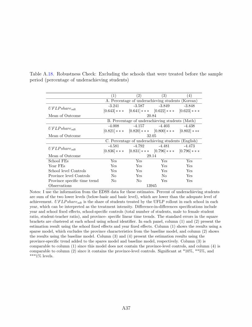
Table A.18. Robustness Check: Excluding the schools that were treated before the sampleperiod (percentage of underachieving students)

(1) (2) (3) (4)

A. Percentage of underachieving students (Korean)

UFLPsharesdt-3.241

[0.643] ∗ ∗ ∗-3.587

[0.641] ∗ ∗ ∗-3.849

[0.622] ∗ ∗ ∗-3.848

[0.623] ∗ ∗ ∗Mean of Outcome 20.84

B. Percentage of underachieving students (Math)

UFLPsharesdt-4.008

[0.821] ∗ ∗ ∗-4.157

[0.820] ∗ ∗ ∗-4.403

[0.800] ∗ ∗ ∗-4.438

[0.802] ∗ ∗∗Mean of Outcome 32.05

C. Percentage of underachieving students (English)

UFLPsharesdt-4.581

[0.836] ∗ ∗ ∗-4.792

[0.831] ∗ ∗ ∗-4.481

[0.796] ∗ ∗ ∗-4.473

[0.796] ∗ ∗ ∗Mean of Outcome 29.14School FEs Yes Yes Yes YesYear FEs Yes Yes Yes YesSchool level Controls Yes Yes Yes YesProvince level Controls No Yes No YesProvince specific time trend No No Yes YesObservations 13945

Notes: I use the information from the EDSS data for these estimates. Percent of underachieving studentsare sum of the two lower levels (below-basic and basic level), which are lower than the adequate level ofachievement. UFLPsharesdt is the share of students treated by the UFLP rollout in each school in eachyear, which can be interpreted as the treatment intensity. Difference-in-differences specifications includeyear and school fixed effects, school-specific controls (total number of students, male to female studentratio, student-teacher ratio), and province- specific linear time trends. The standard errors in the squarebrackets are clustered at each school using school identifier. In each panel, column (1) and (2) present theestimation result using the school fixed effects and year fixed effects. Column (1) shows the results using asparse model, which excludes the province characteristics from the baseline model, and column (2) showsthe results using the baseline model. Column (3) and (4) present the estimation results using theprovince-specific trend added to the spares model and baseline model, respectively. Column (3) iscomparable to column (1) since this model does not contain the province-level controls, and column (4) iscomparable to column (2) since it contains the province-level controls. Significant at *10%, **5%, and***1% levels.

A37

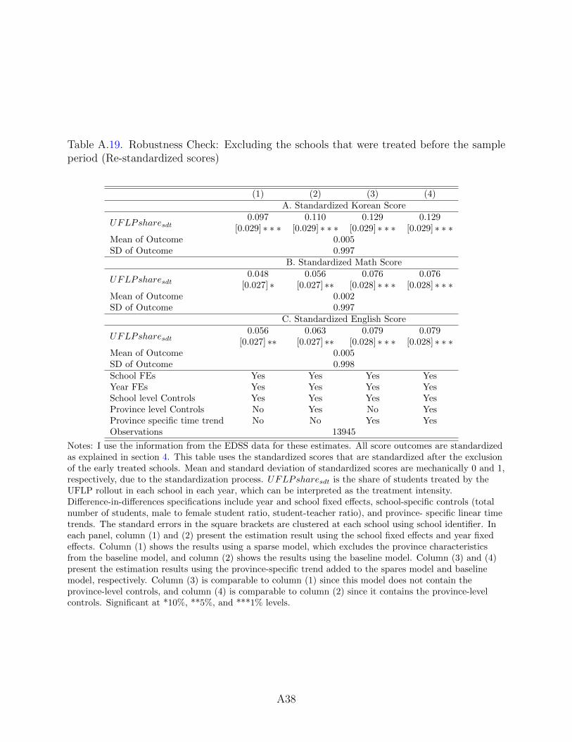
Table A.19. Robustness Check: Excluding the schools that were treated before the sampleperiod (Re-standardized scores)

(1) (2) (3) (4)

A. Standardized Korean Score

UFLPsharesdt0.097

[0.029] ∗ ∗ ∗0.110

[0.029] ∗ ∗ ∗0.129

[0.029] ∗ ∗ ∗0.129

[0.029] ∗ ∗ ∗Mean of Outcome 0.005SD of Outcome 0.997

B. Standardized Math Score

UFLPsharesdt0.048

[0.027] ∗0.056

[0.027] ∗∗0.076

[0.028] ∗ ∗ ∗0.076

[0.028] ∗ ∗ ∗Mean of Outcome 0.002SD of Outcome 0.997

C. Standardized English Score

UFLPsharesdt0.056

[0.027] ∗∗0.063

[0.027] ∗∗0.079

[0.028] ∗ ∗ ∗0.079

[0.028] ∗ ∗ ∗Mean of Outcome 0.005SD of Outcome 0.998School FEs Yes Yes Yes YesYear FEs Yes Yes Yes YesSchool level Controls Yes Yes Yes YesProvince level Controls No Yes No YesProvince specific time trend No No Yes YesObservations 13945

Notes: I use the information from the EDSS data for these estimates. All score outcomes are standardizedas explained in section 4. This table uses the standardized scores that are standardized after the exclusionof the early treated schools. Mean and standard deviation of standardized scores are mechanically 0 and 1,respectively, due to the standardization process. UFLPsharesdt is the share of students treated by theUFLP rollout in each school in each year, which can be interpreted as the treatment intensity.Difference-in-differences specifications include year and school fixed effects, school-specific controls (totalnumber of students, male to female student ratio, student-teacher ratio), and province- specific linear timetrends. The standard errors in the square brackets are clustered at each school using school identifier. Ineach panel, column (1) and (2) present the estimation result using the school fixed effects and year fixedeffects. Column (1) shows the results using a sparse model, which excludes the province characteristicsfrom the baseline model, and column (2) shows the results using the baseline model. Column (3) and (4)present the estimation results using the province-specific trend added to the spares model and baselinemodel, respectively. Column (3) is comparable to column (1) since this model does not contain theprovince-level controls, and column (4) is comparable to column (2) since it contains the province-levelcontrols. Significant at *10%, **5%, and ***1% levels.

A38

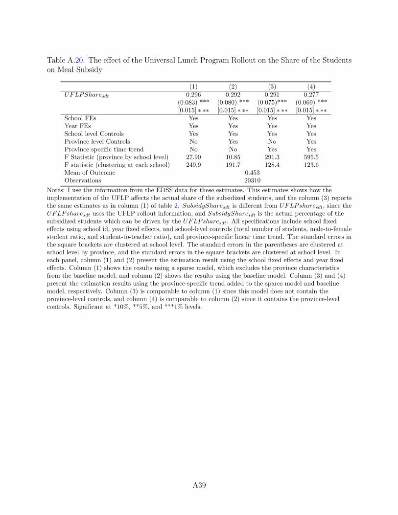
Table A.20. The effect of the Universal Lunch Program Rollout on the Share of the Studentson Meal Subsidy

(1) (2) (3) (4)UFLPSharesdt 0.296 0.292 0.291 0.277

(0.083) *** (0.080) *** (0.075)*** (0.069) ***[0.015] ∗ ∗∗ [0.015] ∗ ∗∗ [0.015] ∗ ∗∗ [0.015] ∗ ∗∗

School FEs Yes Yes Yes YesYear FEs Yes Yes Yes YesSchool level Controls Yes Yes Yes YesProvince level Controls No Yes No YesProvince specific time trend No No Yes YesF Statistic (province by school level) 27.90 10.85 291.3 595.5F statistic (clustering at each school) 249.9 191.7 128.4 123.6Mean of Outcome 0.453Observations 20310

Notes: I use the information from the EDSS data for these estimates. This estimates shows how theimplementation of the UFLP affects the actual share of the subsidized students, and the column (3) reportsthe same estimates as in column (1) of table 2. SubsidySharesdt is different from UFLPsharesdt, since theUFLPsharesdt uses the UFLP rollout information, and SubsidySharesdt is the actual percentage of thesubsidized students which can be driven by the UFLPsharesdt. All specifications include school fixedeffects using school id, year fixed effects, and school-level controls (total number of students, male-to-femalestudent ratio, and student-to-teacher ratio), and province-specific linear time trend. The standard errors inthe square brackets are clustered at school level. The standard errors in the parentheses are clustered atschool level by province, and the standard errors in the square brackets are clustered at school level. Ineach panel, column (1) and (2) present the estimation result using the school fixed effects and year fixedeffects. Column (1) shows the results using a sparse model, which excludes the province characteristicsfrom the baseline model, and column (2) shows the results using the baseline model. Column (3) and (4)present the estimation results using the province-specific trend added to the spares model and baselinemodel, respectively. Column (3) is comparable to column (1) since this model does not contain theprovince-level controls, and column (4) is comparable to column (2) since it contains the province-levelcontrols. Significant at *10%, **5%, and ***1% levels.

A39

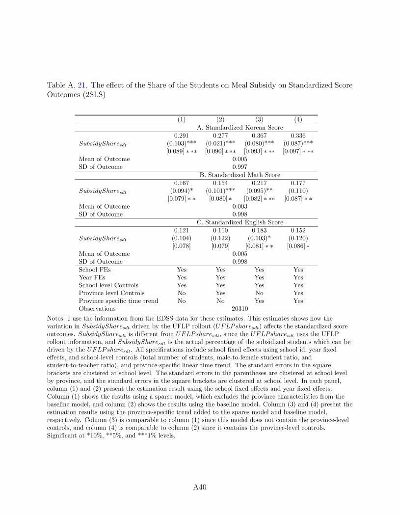
Table A. 21. The effect of the Share of the Students on Meal Subsidy on Standardized ScoreOutcomes (2SLS)

(1) (2) (3) (4)

A. Standardized Korean Score

SubsidySharesdt

0.291(0.103)***[0.089] ∗ ∗∗

0.277(0.021)***[0.090] ∗ ∗∗

0.367(0.080)***[0.093] ∗ ∗∗

0.336(0.087)***[0.097] ∗ ∗∗

Mean of Outcome 0.005SD of Outcome 0.997

B. Standardized Math Score

SubsidySharesdt

0.167(0.094)*

[0.079] ∗ ∗

0.154(0.101)***[0.080] ∗

0.217(0.095)**

[0.082] ∗ ∗∗

0.177(0.110)

[0.087] ∗ ∗Mean of Outcome 0.003SD of Outcome 0.998

C. Standardized English Score

SubsidySharesdt

0.121(0.104)[0.078]

0.110(0.122)[0.079]

0.183(0.103)*

[0.081] ∗ ∗

0.152(0.120)[0.086] ∗

Mean of Outcome 0.005SD of Outcome 0.998School FEs Yes Yes Yes YesYear FEs Yes Yes Yes YesSchool level Controls Yes Yes Yes YesProvince level Controls No Yes No YesProvince specific time trend No No Yes YesObservations 20310

Notes: I use the information from the EDSS data for these estimates. This estimates shows how thevariation in SubsidySharesdt driven by the UFLP rollout (UFLPsharesdt) affects the standardized scoreoutcomes. SubsidySharesdt is different from UFLPsharesdt, since the UFLPsharesdt uses the UFLProllout information, and SubsidySharesdt is the actual percentage of the subsidized students which can bedriven by the UFLPsharesdt. All specifications include school fixed effects using school id, year fixedeffects, and school-level controls (total number of students, male-to-female student ratio, andstudent-to-teacher ratio), and province-specific linear time trend. The standard errors in the squarebrackets are clustered at school level. The standard errors in the parentheses are clustered at school levelby province, and the standard errors in the square brackets are clustered at school level. In each panel,column (1) and (2) present the estimation result using the school fixed effects and year fixed effects.Column (1) shows the results using a sparse model, which excludes the province characteristics from thebaseline model, and column (2) shows the results using the baseline model. Column (3) and (4) present theestimation results using the province-specific trend added to the spares model and baseline model,respectively. Column (3) is comparable to column (1) since this model does not contain the province-levelcontrols, and column (4) is comparable to column (2) since it contains the province-level controls.Significant at *10%, **5%, and ***1% levels.

A40

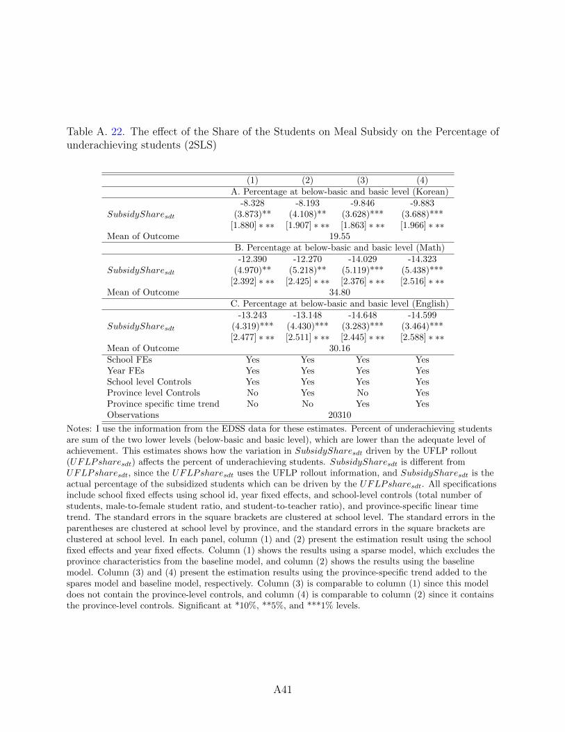
Table A. 22. The effect of the Share of the Students on Meal Subsidy on the Percentage ofunderachieving students (2SLS)

(1) (2) (3) (4)

A. Percentage at below-basic and basic level (Korean)

SubsidySharesdt

-8.328(3.873)**

[1.880] ∗ ∗∗

-8.193(4.108)**

[1.907] ∗ ∗∗

-9.846(3.628)***[1.863] ∗ ∗∗

-9.883(3.688)***[1.966] ∗ ∗∗

Mean of Outcome 19.55B. Percentage at below-basic and basic level (Math)

SubsidySharesdt

-12.390(4.970)**

[2.392] ∗ ∗∗

-12.270(5.218)**

[2.425] ∗ ∗∗

-14.029(5.119)***[2.376] ∗ ∗∗

-14.323(5.438)***[2.516] ∗ ∗∗

Mean of Outcome 34.80C. Percentage at below-basic and basic level (English)

SubsidySharesdt

-13.243(4.319)***[2.477] ∗ ∗∗

-13.148(4.430)***[2.511] ∗ ∗∗

-14.648(3.283)***[2.445] ∗ ∗∗

-14.599(3.464)***[2.588] ∗ ∗∗

Mean of Outcome 30.16School FEs Yes Yes Yes YesYear FEs Yes Yes Yes YesSchool level Controls Yes Yes Yes YesProvince level Controls No Yes No YesProvince specific time trend No No Yes YesObservations 20310

Notes: I use the information from the EDSS data for these estimates. Percent of underachieving studentsare sum of the two lower levels (below-basic and basic level), which are lower than the adequate level ofachievement. This estimates shows how the variation in SubsidySharesdt driven by the UFLP rollout(UFLPsharesdt) affects the percent of underachieving students. SubsidySharesdt is different fromUFLPsharesdt, since the UFLPsharesdt uses the UFLP rollout information, and SubsidySharesdt is theactual percentage of the subsidized students which can be driven by the UFLPsharesdt. All specificationsinclude school fixed effects using school id, year fixed effects, and school-level controls (total number ofstudents, male-to-female student ratio, and student-to-teacher ratio), and province-specific linear timetrend. The standard errors in the square brackets are clustered at school level. The standard errors in theparentheses are clustered at school level by province, and the standard errors in the square brackets areclustered at school level. In each panel, column (1) and (2) present the estimation result using the schoolfixed effects and year fixed effects. Column (1) shows the results using a sparse model, which excludes theprovince characteristics from the baseline model, and column (2) shows the results using the baselinemodel. Column (3) and (4) present the estimation results using the province-specific trend added to thespares model and baseline model, respectively. Column (3) is comparable to column (1) since this modeldoes not contain the province-level controls, and column (4) is comparable to column (2) since it containsthe province-level controls. Significant at *10%, **5%, and ***1% levels.

A41

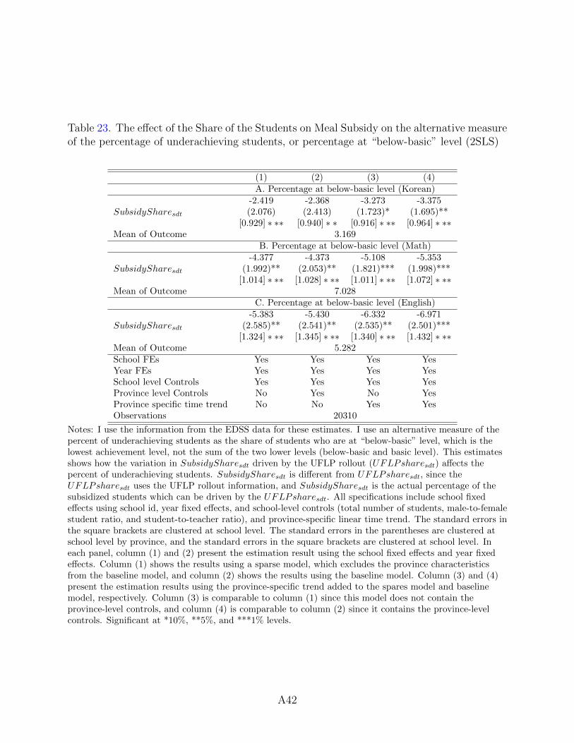
Table 23. The effect of the Share of the Students on Meal Subsidy on the alternative measureof the percentage of underachieving students, or percentage at “below-basic” level (2SLS)

(1) (2) (3) (4)

A. Percentage at below-basic level (Korean)

SubsidySharesdt

-2.419(2.076)

[0.929] ∗ ∗∗

-2.368(2.413)

[0.940] ∗ ∗

-3.273(1.723)*

[0.916] ∗ ∗∗

-3.375(1.695)**

[0.964] ∗ ∗∗Mean of Outcome 3.169

B. Percentage at below-basic level (Math)

SubsidySharesdt

-4.377(1.992)**

[1.014] ∗ ∗∗

-4.373(2.053)**

[1.028] ∗ ∗∗

-5.108(1.821)***[1.011] ∗ ∗∗

-5.353(1.998)***[1.072] ∗ ∗∗

Mean of Outcome 7.028C. Percentage at below-basic level (English)

SubsidySharesdt

-5.383(2.585)**

[1.324] ∗ ∗∗

-5.430(2.541)**

[1.345] ∗ ∗∗

-6.332(2.535)**

[1.340] ∗ ∗∗

-6.971(2.501)***[1.432] ∗ ∗∗

Mean of Outcome 5.282School FEs Yes Yes Yes YesYear FEs Yes Yes Yes YesSchool level Controls Yes Yes Yes YesProvince level Controls No Yes No YesProvince specific time trend No No Yes YesObservations 20310

Notes: I use the information from the EDSS data for these estimates. I use an alternative measure of thepercent of underachieving students as the share of students who are at “below-basic” level, which is thelowest achievement level, not the sum of the two lower levels (below-basic and basic level). This estimatesshows how the variation in SubsidySharesdt driven by the UFLP rollout (UFLPsharesdt) affects thepercent of underachieving students. SubsidySharesdt is different from UFLPsharesdt, since theUFLPsharesdt uses the UFLP rollout information, and SubsidySharesdt is the actual percentage of thesubsidized students which can be driven by the UFLPsharesdt. All specifications include school fixedeffects using school id, year fixed effects, and school-level controls (total number of students, male-to-femalestudent ratio, and student-to-teacher ratio), and province-specific linear time trend. The standard errors inthe square brackets are clustered at school level. The standard errors in the parentheses are clustered atschool level by province, and the standard errors in the square brackets are clustered at school level. Ineach panel, column (1) and (2) present the estimation result using the school fixed effects and year fixedeffects. Column (1) shows the results using a sparse model, which excludes the province characteristicsfrom the baseline model, and column (2) shows the results using the baseline model. Column (3) and (4)present the estimation results using the province-specific trend added to the spares model and baselinemodel, respectively. Column (3) is comparable to column (1) since this model does not contain theprovince-level controls, and column (4) is comparable to column (2) since it contains the province-levelcontrols. Significant at *10%, **5%, and ***1% levels.

A42

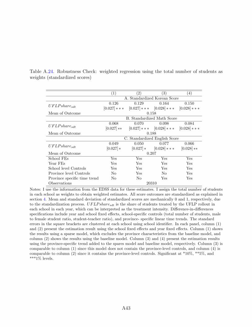
Table A.24. Robustness Check: weighted regression using the total number of students asweights (standardized scores)

(1) (2) (3) (4)

A. Standardized Korean Score

UFLPsharesdt0.126

[0.027] ∗ ∗ ∗0.129

[0.027] ∗ ∗ ∗0.164

[0.028] ∗ ∗ ∗0.150

[0.028] ∗ ∗ ∗Mean of Outcome 0.158

B. Standardized Math Score

UFLPsharesdt0.068

[0.027] ∗∗0.070

[0.027] ∗ ∗ ∗0.098

[0.028] ∗ ∗ ∗0.084

[0.028] ∗ ∗ ∗Mean of Outcome 0.188

C. Standardized English Score

UFLPsharesdt0.049

[0.027] ∗0.050

[0.027] ∗0.077

[0.028] ∗ ∗ ∗0.066

[0.028] ∗∗Mean of Outcome 0.207School FEs Yes Yes Yes YesYear FEs Yes Yes Yes YesSchool level Controls Yes Yes Yes YesProvince level Controls No Yes No YesProvince specific time trend No No Yes YesObservations 20310

Notes: I use the information from the EDSS data for these estimates. I assign the total number of studentsin each school as weights to obtain weighted estimates. All score outcomes are standardized as explained insection 4. Mean and standard deviation of standardized scores are mechanically 0 and 1, respectively, dueto the standardization process. UFLPsharesdt is the share of students treated by the UFLP rollout ineach school in each year, which can be interpreted as the treatment intensity. Difference-in-differencesspecifications include year and school fixed effects, school-specific controls (total number of students, maleto female student ratio, student-teacher ratio), and province- specific linear time trends. The standarderrors in the square brackets are clustered at each school using school identifier. In each panel, column (1)and (2) present the estimation result using the school fixed effects and year fixed effects. Column (1) showsthe results using a sparse model, which excludes the province characteristics from the baseline model, andcolumn (2) shows the results using the baseline model. Column (3) and (4) present the estimation resultsusing the province-specific trend added to the spares model and baseline model, respectively. Column (3) iscomparable to column (1) since this model does not contain the province-level controls, and column (4) iscomparable to column (2) since it contains the province-level controls. Significant at *10%, **5%, and***1% levels.

A43

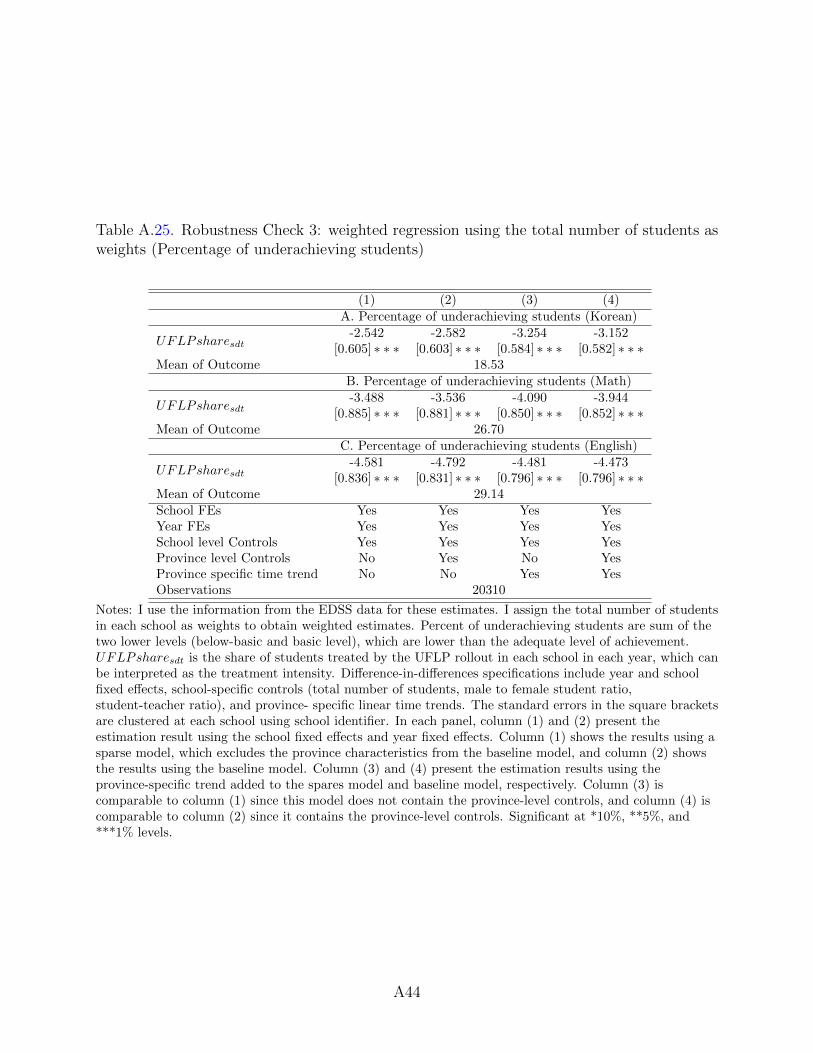
Table A.25. Robustness Check 3: weighted regression using the total number of students asweights (Percentage of underachieving students)

(1) (2) (3) (4)

A. Percentage of underachieving students (Korean)

UFLPsharesdt-2.542

[0.605] ∗ ∗ ∗-2.582

[0.603] ∗ ∗ ∗-3.254

[0.584] ∗ ∗ ∗-3.152

[0.582] ∗ ∗ ∗Mean of Outcome 18.53

B. Percentage of underachieving students (Math)

UFLPsharesdt-3.488

[0.885] ∗ ∗ ∗-3.536

[0.881] ∗ ∗ ∗-4.090

[0.850] ∗ ∗ ∗-3.944

[0.852] ∗ ∗ ∗Mean of Outcome 26.70

C. Percentage of underachieving students (English)

UFLPsharesdt-4.581

[0.836] ∗ ∗ ∗-4.792

[0.831] ∗ ∗ ∗-4.481

[0.796] ∗ ∗ ∗-4.473

[0.796] ∗ ∗ ∗Mean of Outcome 29.14School FEs Yes Yes Yes YesYear FEs Yes Yes Yes YesSchool level Controls Yes Yes Yes YesProvince level Controls No Yes No YesProvince specific time trend No No Yes YesObservations 20310

Notes: I use the information from the EDSS data for these estimates. I assign the total number of studentsin each school as weights to obtain weighted estimates. Percent of underachieving students are sum of thetwo lower levels (below-basic and basic level), which are lower than the adequate level of achievement.UFLPsharesdt is the share of students treated by the UFLP rollout in each school in each year, which canbe interpreted as the treatment intensity. Difference-in-differences specifications include year and schoolfixed effects, school-specific controls (total number of students, male to female student ratio,student-teacher ratio), and province- specific linear time trends. The standard errors in the square bracketsare clustered at each school using school identifier. In each panel, column (1) and (2) present theestimation result using the school fixed effects and year fixed effects. Column (1) shows the results using asparse model, which excludes the province characteristics from the baseline model, and column (2) showsthe results using the baseline model. Column (3) and (4) present the estimation results using theprovince-specific trend added to the spares model and baseline model, respectively. Column (3) iscomparable to column (1) since this model does not contain the province-level controls, and column (4) iscomparable to column (2) since it contains the province-level controls. Significant at *10%, **5%, and***1% levels.

A44

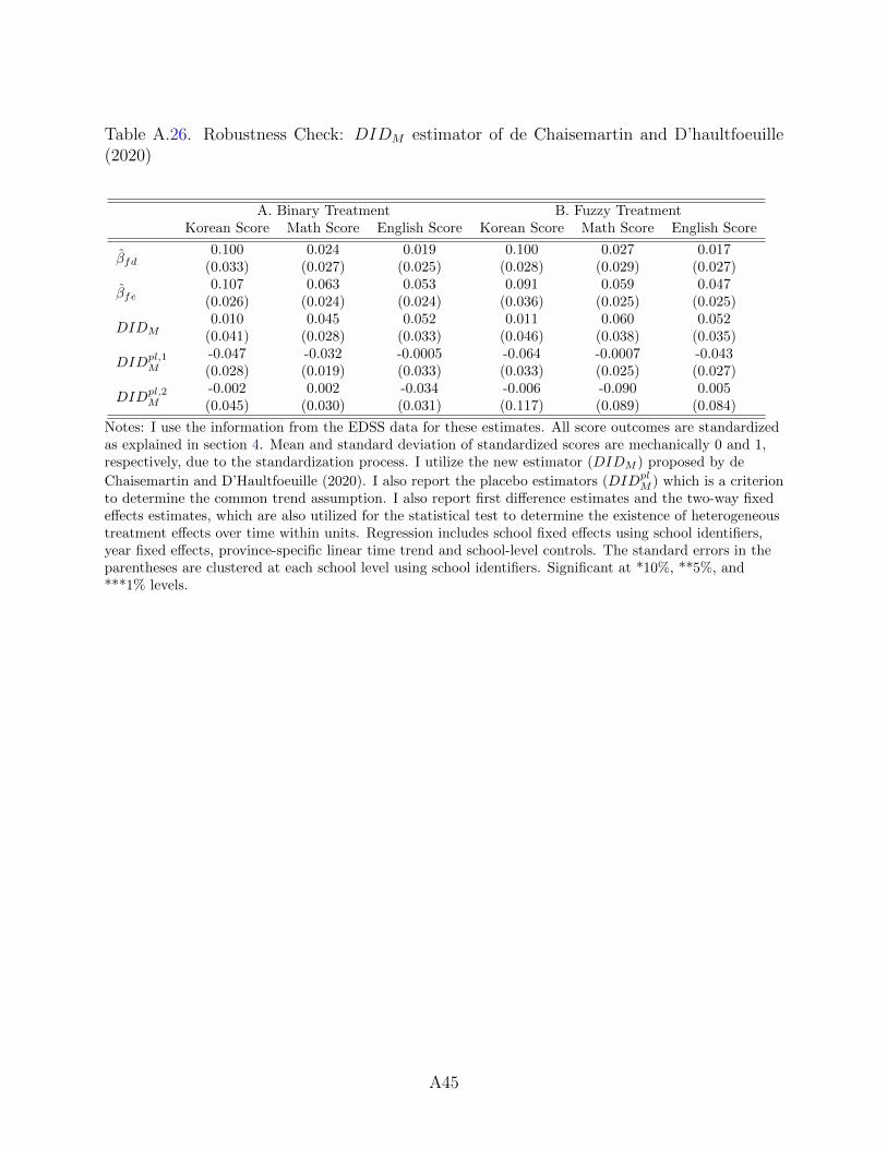
Table A.26. Robustness Check: DIDM estimator of de Chaisemartin and D’haultfoeuille(2020)

A. Binary Treatment B. Fuzzy TreatmentKorean Score Math Score English Score Korean Score Math Score English Score

βfd0.100

(0.033)0.024

(0.027)0.019

(0.025)0.100

(0.028)0.027

(0.029)0.017

(0.027)

βfe0.107

(0.026)0.063

(0.024)0.053

(0.024)0.091

(0.036)0.059

(0.025)0.047

(0.025)

DIDM0.010

(0.041)0.045

(0.028)0.052

(0.033)0.011

(0.046)0.060

(0.038)0.052

(0.035)

DIDpl,1M

-0.047(0.028)

-0.032(0.019)

-0.0005(0.033)

-0.064(0.033)

-0.0007(0.025)

-0.043(0.027)

DIDpl,2M

-0.002(0.045)

0.002(0.030)

-0.034(0.031)

-0.006(0.117)

-0.090(0.089)

0.005(0.084)

Notes: I use the information from the EDSS data for these estimates. All score outcomes are standardizedas explained in section 4. Mean and standard deviation of standardized scores are mechanically 0 and 1,respectively, due to the standardization process. I utilize the new estimator (DIDM ) proposed by de

Chaisemartin and D’Haultfoeuille (2020). I also report the placebo estimators (DIDplM ) which is a criterion

to determine the common trend assumption. I also report first difference estimates and the two-way fixedeffects estimates, which are also utilized for the statistical test to determine the existence of heterogeneoustreatment effects over time within units. Regression includes school fixed effects using school identifiers,year fixed effects, province-specific linear time trend and school-level controls. The standard errors in theparentheses are clustered at each school level using school identifiers. Significant at *10%, **5%, and***1% levels.

A45

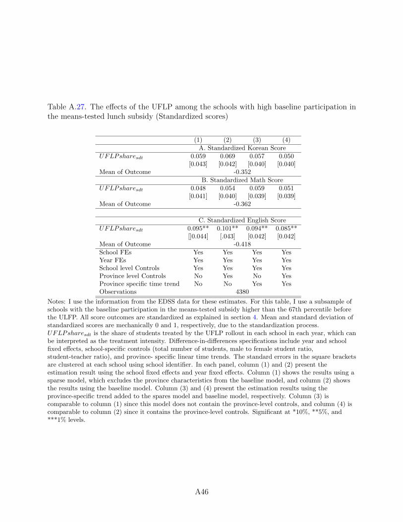
Table A.27. The effects of the UFLP among the schools with high baseline participation inthe means-tested lunch subsidy (Standardized scores)

(1) (2) (3) (4)A. Standardized Korean Score

UFLPsharesdt 0.059 0.069 0.057 0.050[0.043] [0.042] [0.040] [0.040]

Mean of Outcome -0.352B. Standardized Math Score

UFLPsharesdt 0.048 0.054 0.059 0.051[0.041] [0.040] [0.039] [0.039]

Mean of Outcome -0.362

C. Standardized English ScoreUFLPsharesdt 0.095** 0.101** 0.094** 0.085**

[]0.044] [.043] [0.042] [0.042]Mean of Outcome -0.418School FEs Yes Yes Yes YesYear FEs Yes Yes Yes YesSchool level Controls Yes Yes Yes YesProvince level Controls No Yes No YesProvince specific time trend No No Yes YesObservations 4380

Notes: I use the information from the EDSS data for these estimates. For this table, I use a subsample ofschools with the baseline participation in the means-tested subsidy higher than the 67th percentile beforethe ULFP. All score outcomes are standardized as explained in section 4. Mean and standard deviation ofstandardized scores are mechanically 0 and 1, respectively, due to the standardization process.UFLPsharesdt is the share of students treated by the UFLP rollout in each school in each year, which canbe interpreted as the treatment intensity. Difference-in-differences specifications include year and schoolfixed effects, school-specific controls (total number of students, male to female student ratio,student-teacher ratio), and province- specific linear time trends. The standard errors in the square bracketsare clustered at each school using school identifier. In each panel, column (1) and (2) present theestimation result using the school fixed effects and year fixed effects. Column (1) shows the results using asparse model, which excludes the province characteristics from the baseline model, and column (2) showsthe results using the baseline model. Column (3) and (4) present the estimation results using theprovince-specific trend added to the spares model and baseline model, respectively. Column (3) iscomparable to column (1) since this model does not contain the province-level controls, and column (4) iscomparable to column (2) since it contains the province-level controls. Significant at *10%, **5%, and***1% levels.

A46

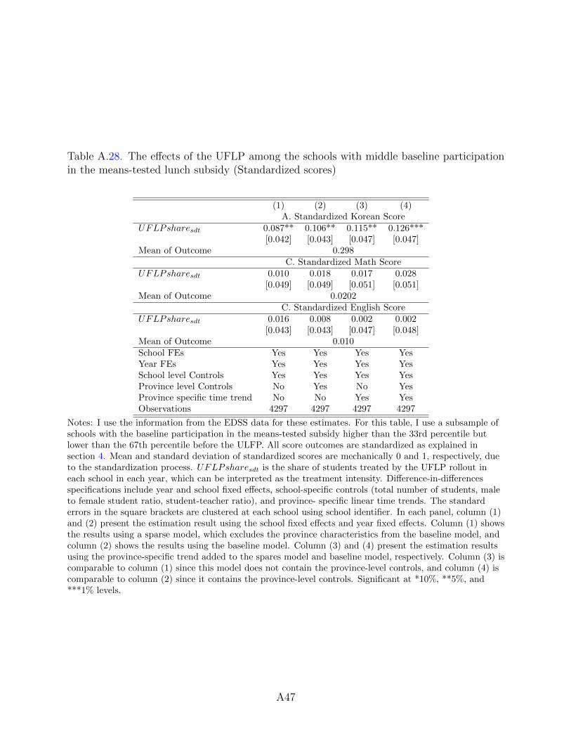
Table A.28. The effects of the UFLP among the schools with middle baseline participationin the means-tested lunch subsidy (Standardized scores)

(1) (2) (3) (4)A. Standardized Korean Score

UFLPsharesdt 0.087** 0.106** 0.115** 0.126***[0.042] [0.043] [0.047] [0.047]

Mean of Outcome 0.298C. Standardized Math Score

UFLPsharesdt 0.010 0.018 0.017 0.028[0.049] [0.049] [0.051] [0.051]

Mean of Outcome 0.0202C. Standardized English Score

UFLPsharesdt 0.016 0.008 0.002 0.002[0.043] [0.043] [0.047] [0.048]

Mean of Outcome 0.010School FEs Yes Yes Yes YesYear FEs Yes Yes Yes YesSchool level Controls Yes Yes Yes YesProvince level Controls No Yes No YesProvince specific time trend No No Yes YesObservations 4297 4297 4297 4297

Notes: I use the information from the EDSS data for these estimates. For this table, I use a subsample ofschools with the baseline participation in the means-tested subsidy higher than the 33rd percentile butlower than the 67th percentile before the ULFP. All score outcomes are standardized as explained insection 4. Mean and standard deviation of standardized scores are mechanically 0 and 1, respectively, dueto the standardization process. UFLPsharesdt is the share of students treated by the UFLP rollout ineach school in each year, which can be interpreted as the treatment intensity. Difference-in-differencesspecifications include year and school fixed effects, school-specific controls (total number of students, maleto female student ratio, student-teacher ratio), and province- specific linear time trends. The standarderrors in the square brackets are clustered at each school using school identifier. In each panel, column (1)and (2) present the estimation result using the school fixed effects and year fixed effects. Column (1) showsthe results using a sparse model, which excludes the province characteristics from the baseline model, andcolumn (2) shows the results using the baseline model. Column (3) and (4) present the estimation resultsusing the province-specific trend added to the spares model and baseline model, respectively. Column (3) iscomparable to column (1) since this model does not contain the province-level controls, and column (4) iscomparable to column (2) since it contains the province-level controls. Significant at *10%, **5%, and***1% levels.

A47

Table A.29. The effects of the UFLP among the schools with low baseline participation inthe means-tested lunch subsidy (Standardized scores)

(1) (2) (3) (4)A. Standardized Korean Score

UFLPsharesdt 0.047 0.097 0.124** 0.139**[0.058] [0.059] [0.058] [0.058]

Mean of Outcome 0.598A. Standardized Math Score

UFLPsharesdt 0.007 0.043 0.082 0.096[0.056] [0.056] [0.062] [0.062]

Mean of Outcome 0.663A. Standardized English Score

UFLPsharesdt -0.040 -0.005 0.030 0.045[0.056] [0.057] [0.062] [0.062]

Mean of Outcome 0.698School FEs Yes Yes Yes YesYear FEs Yes Yes Yes YesSchool level Controls Yes Yes Yes YesProvince level Controls No Yes No YesProvince specific time trend No No Yes YesObservations 4168

Notes: I use the information from the EDSS data for these estimates. For this table, I use a subsample ofschools with the baseline participation in the means-tested subsidy lower than the 33rd percentile beforethe ULFP. All score outcomes are standardized as explained in section 4. Mean and standard deviation ofstandardized scores are mechanically 0 and 1, respectively, due to the standardization process.UFLPsharesdt is the share of students treated by the UFLP rollout in each school in each year, which canbe interpreted as the treatment intensity. Difference-in-differences specifications include year and schoolfixed effects, school-specific controls (total number of students, male to female student ratio,student-teacher ratio), and province- specific linear time trends. The standard errors in the square bracketsare clustered at each school using school identifier. In each panel, column (1) and (2) present theestimation result using the school fixed effects and year fixed effects. Column (1) shows the results using asparse model, which excludes the province characteristics from the baseline model, and column (2) showsthe results using the baseline model. Column (3) and (4) present the estimation results using theprovince-specific trend added to the spares model and baseline model, respectively. Column (3) iscomparable to column (1) since this model does not contain the province-level controls, and column (4) iscomparable to column (2) since it contains the province-level controls. Significant at *10%, **5%, and***1% levels.

A48

Table A.30. The effects of the UFLP among the schools with high baseline participation inthe means-tested lunch subsidy (percentage of underachieving students)

Percentage of Underachieving students(1) (2) (3) (4)

A. Korean

UFLPsharesdt-2.192*[1.136]

-2.415**[1.125]

-3.265***[1.065]

-3.027***[1.078]

Mean of Outcome 30.26B. Math

UFLPsharesdt-2.597***

[1.345]-2.615*[1.338]

-3.634***[1.296]

-3.407***[1.295]

Mean of Outcome 44.75C. English

UFLPsharesdt-1.580[1.325]

-1.727[1.313]

-1.933[1.226]

-1.637[1.235]

Mean of Outcome 42.19School FEs Yes Yes Yes YesYear FEs Yes Yes Yes YesSchool level Controls Yes Yes Yes YesProvince level Controls No Yes No YesProvince specific time trend No No Yes YesObservations 4297

Notes: I use the information from the EDSS data for these estimates. For this table, I use a subsample ofschools with the baseline participation in the means-tested subsidy higher than the 67th percentile beforethe ULFP. Percent of underachieving students are sum of the two lower levels (below-basic and basic level),which are lower than the adequate level of achievement. UFLPsharesdt is the share of students treated bythe UFLP rollout in each school in each year, which can be interpreted as the treatment intensity.Difference-in-differences specifications include year and school fixed effects, school-specific controls (totalnumber of students, male to female student ratio, student-teacher ratio), and province- specific linear timetrends. The standard errors in the square brackets are clustered at each school using school identifier. Ineach panel, column (1) and (2) present the estimation result using the school fixed effects and year fixedeffects. Column (1) shows the results using a sparse model, which excludes the province characteristicsfrom the baseline model, and column (2) shows the results using the baseline model. Column (3) and (4)present the estimation results using the province-specific trend added to the spares model and baselinemodel, respectively. Column (3) is comparable to column (1) since this model does not contain theprovince-level controls, and column (4) is comparable to column (2) since it contains the province-levelcontrols. Significant at *10%, **5%, and ***1% levels.

A49

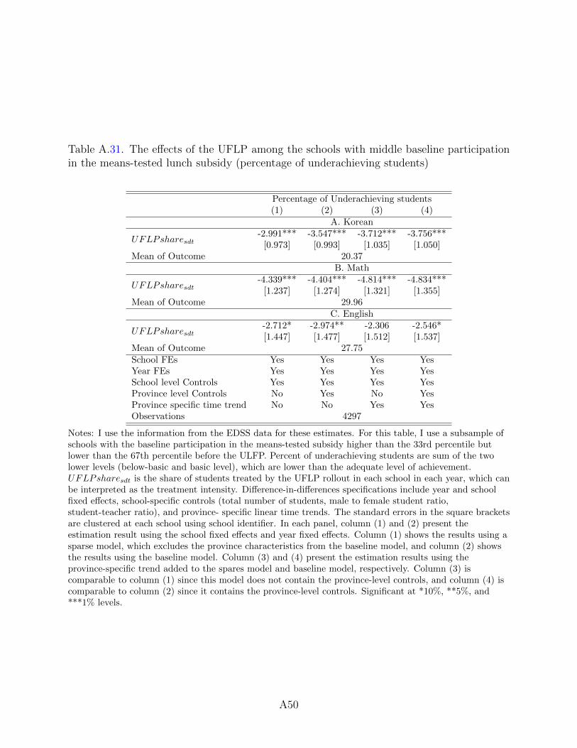
Table A.31. The effects of the UFLP among the schools with middle baseline participationin the means-tested lunch subsidy (percentage of underachieving students)

Percentage of Underachieving students(1) (2) (3) (4)

A. Korean

UFLPsharesdt-2.991***

[0.973]-3.547***

[0.993]-3.712***

[1.035]-3.756***

[1.050]Mean of Outcome 20.37

B. Math

UFLPsharesdt-4.339***

[1.237]-4.404***

[1.274]-4.814***

[1.321]-4.834***

[1.355]Mean of Outcome 29.96

C. English

UFLPsharesdt-2.712*[1.447]

-2.974**[1.477]

-2.306[1.512]

-2.546*[1.537]

Mean of Outcome 27.75School FEs Yes Yes Yes YesYear FEs Yes Yes Yes YesSchool level Controls Yes Yes Yes YesProvince level Controls No Yes No YesProvince specific time trend No No Yes YesObservations 4297

Notes: I use the information from the EDSS data for these estimates. For this table, I use a subsample ofschools with the baseline participation in the means-tested subsidy higher than the 33rd percentile butlower than the 67th percentile before the ULFP. Percent of underachieving students are sum of the twolower levels (below-basic and basic level), which are lower than the adequate level of achievement.UFLPsharesdt is the share of students treated by the UFLP rollout in each school in each year, which canbe interpreted as the treatment intensity. Difference-in-differences specifications include year and schoolfixed effects, school-specific controls (total number of students, male to female student ratio,student-teacher ratio), and province- specific linear time trends. The standard errors in the square bracketsare clustered at each school using school identifier. In each panel, column (1) and (2) present theestimation result using the school fixed effects and year fixed effects. Column (1) shows the results using asparse model, which excludes the province characteristics from the baseline model, and column (2) showsthe results using the baseline model. Column (3) and (4) present the estimation results using theprovince-specific trend added to the spares model and baseline model, respectively. Column (3) iscomparable to column (1) since this model does not contain the province-level controls, and column (4) iscomparable to column (2) since it contains the province-level controls. Significant at *10%, **5%, and***1% levels.

A50

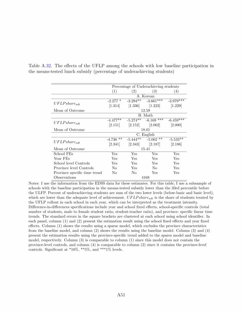
Table A.32. The effects of the UFLP among the schools with low baseline participation inthe means-tested lunch subsidy (percentage of underachieving students)

Percentage of Underachieving students(1) (2) (3) (4)

A. Korean

UFLPsharesdt-2.277 *[1.314]

-3.294**[1.336]

-3.661***[1.223]

-3.979***[1.229]

Mean of Outcome 12.59B. Math

UFLPsharesdt-4.477**[2.151]

-5.274**[2.152]

-6.169 ***[2.002]

-6.459***[2.000]

Mean of Outcome 18.01C. English

UFLPsharesdt-4.736 **

[2.341]-5.444**[2.343]

-5.002 **[2.187]

-5.533**[2.186]

Mean of Outcome 15.41School FEs Yes Yes Yes YesYear FEs Yes Yes Yes YesSchool level Controls Yes Yes Yes YesProvince level Controls No Yes No YesProvince specific time trend No No Yes YesObservations 4168

Notes: I use the information from the EDSS data for these estimates. For this table, I use a subsample ofschools with the baseline participation in the means-tested subsidy lower than the 33rd percentile beforethe ULFP. Percent of underachieving students are sum of the two lower levels (below-basic and basic level),which are lower than the adequate level of achievement. UFLPsharesdt is the share of students treated bythe UFLP rollout in each school in each year, which can be interpreted as the treatment intensity.Difference-in-differences specifications include year and school fixed effects, school-specific controls (totalnumber of students, male to female student ratio, student-teacher ratio), and province- specific linear timetrends. The standard errors in the square brackets are clustered at each school using school identifier. Ineach panel, column (1) and (2) present the estimation result using the school fixed effects and year fixedeffects. Column (1) shows the results using a sparse model, which excludes the province characteristicsfrom the baseline model, and column (2) shows the results using the baseline model. Column (3) and (4)present the estimation results using the province-specific trend added to the spares model and baselinemodel, respectively. Column (3) is comparable to column (1) since this model does not contain theprovince-level controls, and column (4) is comparable to column (2) since it contains the province-levelcontrols. Significant at *10%, **5%, and ***1% levels.

A51

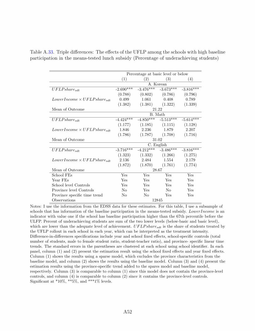
Table A.33. Triple differences: The effects of the UFLP among the schools with high baselineparticipation in the means-tested lunch subsidy (Percentage of underachieving students)

Percentage at basic level or below(1) (2) (3) (4)

A. KoreanUFLPsharesdt -2.690*** -3.476*** -3.673*** -3.816***

(0.788) (0.802) (0.786) (0.796)LowerIncome× UFLPsharesdt 0.499 1.061 0.408 0.789

(1.382) (1.381) (1.322) (1.339)Mean of Outcome 21.22

B. MathUFLPsharesdt -4.424*** -4.850*** -5.513*** -5.614***

(1.177) (1.185) (1.115) (1.128)LowerIncome× UFLPsharesdt 1.846 2.236 1.879 2.207

(1.786) (1.787) (1.708) (1.716)Mean of Outcome 31.02

C. EnglishUFLPsharesdt -3.716*** -4.212*** -3.486*** -3.816***

(1.323) (1.332) (1.266) (1.275)LowerIncome× UFLPsharesdt 2.136 2.484 1.554 2.179

(1.872) (1.870) (1.761) (1.774)Mean of Outcome 28.67School FEs Yes Yes Yes YesYear FEs Yes Yes Yes YesSchool level Controls Yes Yes Yes YesProvince level Controls No Yes No YesProvince specific time trend No No Yes YesObservations 12845

Notes: I use the information from the EDSS data for these estimates. For this table, I use a subsample ofschools that has information of the baseline participation in the means-tested subsidy. LowerIncome is anindicator with value one if the school has baseline participation higher than the 67th percentile before theULFP. Percent of underachieving students are sum of the two lower levels (below-basic and basic level),which are lower than the adequate level of achievement. UFLPsharesdt is the share of students treated bythe UFLP rollout in each school in each year, which can be interpreted as the treatment intensity.Difference-in-differences specifications include year and school fixed effects, school-specific controls (totalnumber of students, male to female student ratio, student-teacher ratio), and province- specific linear timetrends. The standard errors in the parentheses are clustered at each school using school identifier. In eachpanel, column (1) and (2) present the estimation result using the school fixed effects and year fixed effects.Column (1) shows the results using a sparse model, which excludes the province characteristics from thebaseline model, and column (2) shows the results using the baseline model. Column (3) and (4) present theestimation results using the province-specific trend added to the spares model and baseline model,respectively. Column (3) is comparable to column (1) since this model does not contain the province-levelcontrols, and column (4) is comparable to column (2) since it contains the province-level controls.Significant at *10%, **5%, and ***1% levels.

A52

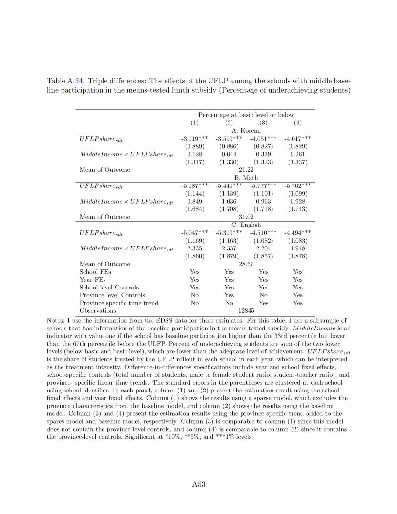
Table A.34. Triple differences: The effects of the UFLP among the schools with middle base-line participation in the means-tested lunch subsidy (Percentage of underachieving students)

Percentage at basic level or below(1) (2) (3) (4)

A. KoreanUFLPsharesdt -3.119*** -3.590*** -4.051*** -4.017***

(0.889) (0.886) (0.827) (0.829)MiddleIncome× UFLPsharesdt 0.128 0.044 0.339 0.261

(1.317) (1.330) (1.323) (1.337)Mean of Outcome 21.22

B. MathUFLPsharesdt -5.187*** -5.440*** -5.777*** -5.762***

(1.144) (1.139) (1.101) (1.099)MiddleIncome× UFLPsharesdt 0.849 1.036 0.963 0.928

(1.684) (1.708) (1.718) (1.743)Mean of Outcome 31.02

C. EnglishUFLPsharesdt -5.047*** -5.310*** -4.510*** -4.494***

(1.169) (1.163) (1.082) (1.083)MiddleIncome× UFLPsharesdt 2.335 2.337 2.204 1.948

(1.860) (1.879) (1.857) (1.878)Mean of Outcome 28.67School FEs Yes Yes Yes YesYear FEs Yes Yes Yes YesSchool level Controls Yes Yes Yes YesProvince level Controls No Yes No YesProvince specific time trend No No Yes YesObservations 12845

Notes: I use the information from the EDSS data for these estimates. For this table, I use a subsample ofschools that has information of the baseline participation in the means-tested subsidy. MiddleIncome is anindicator with value one if the school has baseline participation higher than the 33rd percentile but lowerthan the 67th percentile before the ULFP. Percent of underachieving students are sum of the two lowerlevels (below-basic and basic level), which are lower than the adequate level of achievement. UFLPsharesdtis the share of students treated by the UFLP rollout in each school in each year, which can be interpretedas the treatment intensity. Difference-in-differences specifications include year and school fixed effects,school-specific controls (total number of students, male to female student ratio, student-teacher ratio), andprovince- specific linear time trends. The standard errors in the parentheses are clustered at each schoolusing school identifier. In each panel, column (1) and (2) present the estimation result using the schoolfixed effects and year fixed effects. Column (1) shows the results using a sparse model, which excludes theprovince characteristics from the baseline model, and column (2) shows the results using the baselinemodel. Column (3) and (4) present the estimation results using the province-specific trend added to thespares model and baseline model, respectively. Column (3) is comparable to column (1) since this modeldoes not contain the province-level controls, and column (4) is comparable to column (2) since it containsthe province-level controls. Significant at *10%, **5%, and ***1% levels.

A53

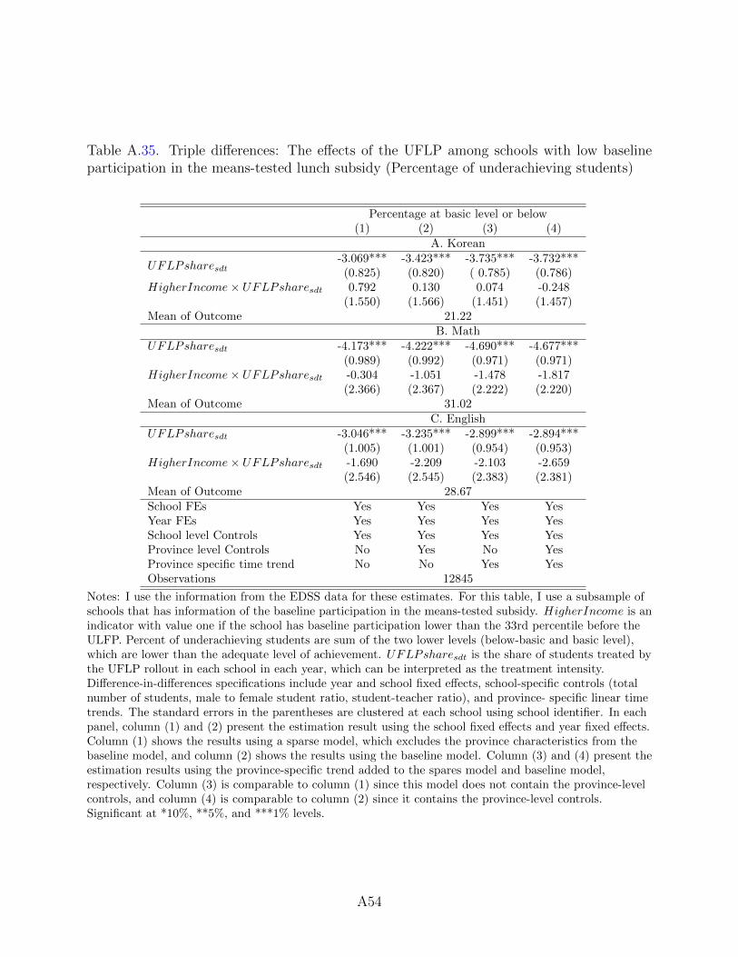
Table A.35. Triple differences: The effects of the UFLP among schools with low baselineparticipation in the means-tested lunch subsidy (Percentage of underachieving students)

Percentage at basic level or below(1) (2) (3) (4)

A. Korean

UFLPsharesdt-3.069***(0.825)

-3.423***(0.820)

-3.735***( 0.785)

-3.732***(0.786)

HigherIncome× UFLPsharesdt 0.792 0.130 0.074 -0.248(1.550) (1.566) (1.451) (1.457)

Mean of Outcome 21.22B. Math

UFLPsharesdt -4.173*** -4.222*** -4.690*** -4.677***(0.989) (0.992) (0.971) (0.971)

HigherIncome× UFLPsharesdt -0.304 -1.051 -1.478 -1.817(2.366) (2.367) (2.222) (2.220)

Mean of Outcome 31.02C. English

UFLPsharesdt -3.046*** -3.235*** -2.899*** -2.894***(1.005) (1.001) (0.954) (0.953)

HigherIncome× UFLPsharesdt -1.690 -2.209 -2.103 -2.659(2.546) (2.545) (2.383) (2.381)

Mean of Outcome 28.67School FEs Yes Yes Yes YesYear FEs Yes Yes Yes YesSchool level Controls Yes Yes Yes YesProvince level Controls No Yes No YesProvince specific time trend No No Yes YesObservations 12845

Notes: I use the information from the EDSS data for these estimates. For this table, I use a subsample ofschools that has information of the baseline participation in the means-tested subsidy. HigherIncome is anindicator with value one if the school has baseline participation lower than the 33rd percentile before theULFP. Percent of underachieving students are sum of the two lower levels (below-basic and basic level),which are lower than the adequate level of achievement. UFLPsharesdt is the share of students treated bythe UFLP rollout in each school in each year, which can be interpreted as the treatment intensity.Difference-in-differences specifications include year and school fixed effects, school-specific controls (totalnumber of students, male to female student ratio, student-teacher ratio), and province- specific linear timetrends. The standard errors in the parentheses are clustered at each school using school identifier. In eachpanel, column (1) and (2) present the estimation result using the school fixed effects and year fixed effects.Column (1) shows the results using a sparse model, which excludes the province characteristics from thebaseline model, and column (2) shows the results using the baseline model. Column (3) and (4) present theestimation results using the province-specific trend added to the spares model and baseline model,respectively. Column (3) is comparable to column (1) since this model does not contain the province-levelcontrols, and column (4) is comparable to column (2) since it contains the province-level controls.Significant at *10%, **5%, and ***1% levels.

A54

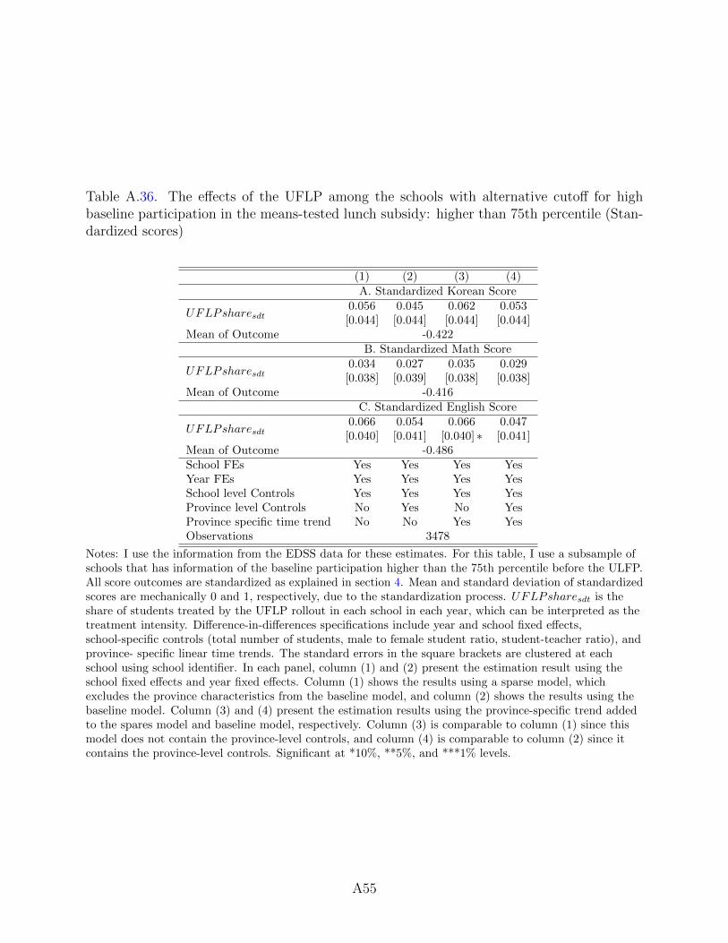
Table A.36. The effects of the UFLP among the schools with alternative cutoff for highbaseline participation in the means-tested lunch subsidy: higher than 75th percentile (Stan-dardized scores)

(1) (2) (3) (4)

A. Standardized Korean Score

UFLPsharesdt0.056[0.044]

0.045[0.044]

0.062[0.044]

0.053[0.044]

Mean of Outcome -0.422B. Standardized Math Score

UFLPsharesdt0.034[0.038]

0.027[0.039]

0.035[0.038]

0.029[0.038]

Mean of Outcome -0.416C. Standardized English Score

UFLPsharesdt0.066[0.040]

0.054[0.041]

0.066[0.040] ∗

0.047[0.041]

Mean of Outcome -0.486School FEs Yes Yes Yes YesYear FEs Yes Yes Yes YesSchool level Controls Yes Yes Yes YesProvince level Controls No Yes No YesProvince specific time trend No No Yes YesObservations 3478

Notes: I use the information from the EDSS data for these estimates. For this table, I use a subsample ofschools that has information of the baseline participation higher than the 75th percentile before the ULFP.All score outcomes are standardized as explained in section 4. Mean and standard deviation of standardizedscores are mechanically 0 and 1, respectively, due to the standardization process. UFLPsharesdt is theshare of students treated by the UFLP rollout in each school in each year, which can be interpreted as thetreatment intensity. Difference-in-differences specifications include year and school fixed effects,school-specific controls (total number of students, male to female student ratio, student-teacher ratio), andprovince- specific linear time trends. The standard errors in the square brackets are clustered at eachschool using school identifier. In each panel, column (1) and (2) present the estimation result using theschool fixed effects and year fixed effects. Column (1) shows the results using a sparse model, whichexcludes the province characteristics from the baseline model, and column (2) shows the results using thebaseline model. Column (3) and (4) present the estimation results using the province-specific trend addedto the spares model and baseline model, respectively. Column (3) is comparable to column (1) since thismodel does not contain the province-level controls, and column (4) is comparable to column (2) since itcontains the province-level controls. Significant at *10%, **5%, and ***1% levels.

A55

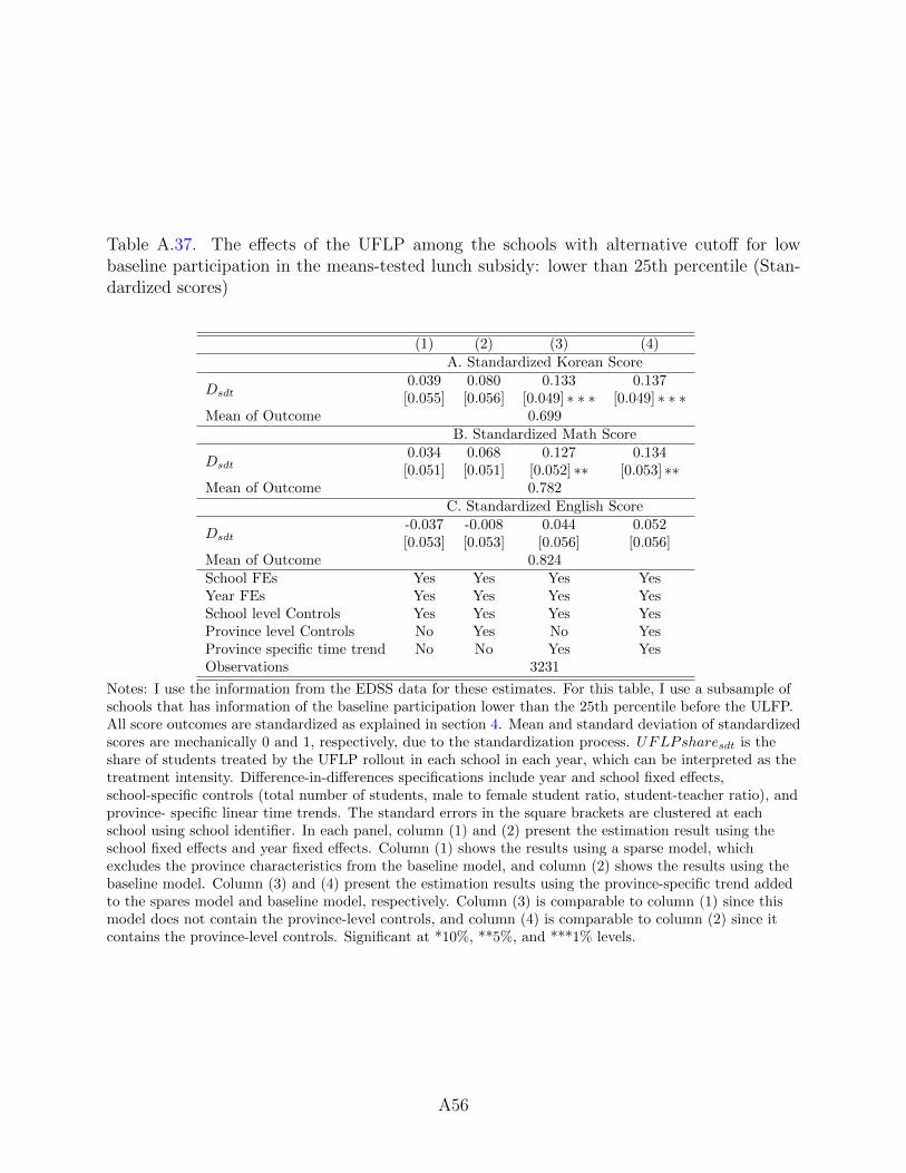
Table A.37. The effects of the UFLP among the schools with alternative cutoff for lowbaseline participation in the means-tested lunch subsidy: lower than 25th percentile (Stan-dardized scores)

(1) (2) (3) (4)

A. Standardized Korean Score

Dsdt0.039[0.055]

0.080[0.056]

0.133[0.049] ∗ ∗ ∗

0.137[0.049] ∗ ∗ ∗

Mean of Outcome 0.699B. Standardized Math Score

Dsdt0.034[0.051]

0.068[0.051]

0.127[0.052] ∗∗

0.134[0.053] ∗∗

Mean of Outcome 0.782C. Standardized English Score

Dsdt-0.037[0.053]

-0.008[0.053]

0.044[0.056]

0.052[0.056]

Mean of Outcome 0.824School FEs Yes Yes Yes YesYear FEs Yes Yes Yes YesSchool level Controls Yes Yes Yes YesProvince level Controls No Yes No YesProvince specific time trend No No Yes YesObservations 3231

Notes: I use the information from the EDSS data for these estimates. For this table, I use a subsample ofschools that has information of the baseline participation lower than the 25th percentile before the ULFP.All score outcomes are standardized as explained in section 4. Mean and standard deviation of standardizedscores are mechanically 0 and 1, respectively, due to the standardization process. UFLPsharesdt is theshare of students treated by the UFLP rollout in each school in each year, which can be interpreted as thetreatment intensity. Difference-in-differences specifications include year and school fixed effects,school-specific controls (total number of students, male to female student ratio, student-teacher ratio), andprovince- specific linear time trends. The standard errors in the square brackets are clustered at eachschool using school identifier. In each panel, column (1) and (2) present the estimation result using theschool fixed effects and year fixed effects. Column (1) shows the results using a sparse model, whichexcludes the province characteristics from the baseline model, and column (2) shows the results using thebaseline model. Column (3) and (4) present the estimation results using the province-specific trend addedto the spares model and baseline model, respectively. Column (3) is comparable to column (1) since thismodel does not contain the province-level controls, and column (4) is comparable to column (2) since itcontains the province-level controls. Significant at *10%, **5%, and ***1% levels.

A56

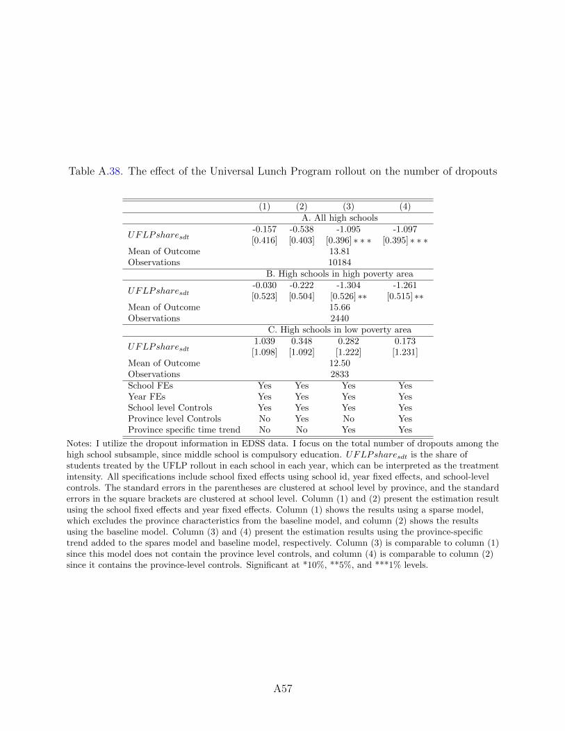
Table A.38. The effect of the Universal Lunch Program rollout on the number of dropouts

(1) (2) (3) (4)

A. All high schools

UFLPsharesdt-0.157[0.416]

-0.538[0.403]

-1.095[0.396] ∗ ∗ ∗

-1.097[0.395] ∗ ∗ ∗

Mean of Outcome 13.81Observations 10184

B. High schools in high poverty area

UFLPsharesdt-0.030[0.523]

-0.222[0.504]

-1.304[0.526] ∗∗

-1.261[0.515] ∗∗

Mean of Outcome 15.66Observations 2440

C. High schools in low poverty area

UFLPsharesdt1.039[1.098]

0.348[1.092]

0.282[1.222]

0.173[1.231]

Mean of Outcome 12.50Observations 2833School FEs Yes Yes Yes YesYear FEs Yes Yes Yes YesSchool level Controls Yes Yes Yes YesProvince level Controls No Yes No YesProvince specific time trend No No Yes Yes

Notes: I utilize the dropout information in EDSS data. I focus on the total number of dropouts among thehigh school subsample, since middle school is compulsory education. UFLPsharesdt is the share ofstudents treated by the UFLP rollout in each school in each year, which can be interpreted as the treatmentintensity. All specifications include school fixed effects using school id, year fixed effects, and school-levelcontrols. The standard errors in the parentheses are clustered at school level by province, and the standarderrors in the square brackets are clustered at school level. Column (1) and (2) present the estimation resultusing the school fixed effects and year fixed effects. Column (1) shows the results using a sparse model,which excludes the province characteristics from the baseline model, and column (2) shows the resultsusing the baseline model. Column (3) and (4) present the estimation results using the province-specifictrend added to the spares model and baseline model, respectively. Column (3) is comparable to column (1)since this model does not contain the province level controls, and column (4) is comparable to column (2)since it contains the province-level controls. Significant at *10%, **5%, and ***1% levels.

A57

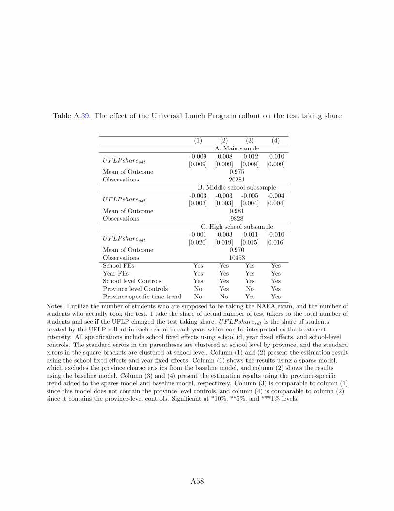
Table A.39. The effect of the Universal Lunch Program rollout on the test taking share

(1) (2) (3) (4)

A. Main sample

UFLPsharesdt-0.009[0.009]

-0.008[0.009]

-0.012[0.008]

-0.010[0.009]

Mean of Outcome 0.975Observations 20281

B. Middle school subsample

UFLPsharesdt-0.003[0.003]

-0.003[0.003]

-0.005[0.004]

-0.004[0.004]

Mean of Outcome 0.981Observations 9828

C. High school subsample

UFLPsharesdt-0.001[0.020]

-0.003[0.019]

-0.011[0.015]

-0.010[0.016]

Mean of Outcome 0.970Observations 10453School FEs Yes Yes Yes YesYear FEs Yes Yes Yes YesSchool level Controls Yes Yes Yes YesProvince level Controls No Yes No YesProvince specific time trend No No Yes Yes

Notes: I utilize the number of students who are supposed to be taking the NAEA exam, and the number ofstudents who actually took the test. I take the share of actual number of test takers to the total number ofstudents and see if the UFLP changed the test taking share. UFLPsharesdt is the share of studentstreated by the UFLP rollout in each school in each year, which can be interpreted as the treatmentintensity. All specifications include school fixed effects using school id, year fixed effects, and school-levelcontrols. The standard errors in the parentheses are clustered at school level by province, and the standarderrors in the square brackets are clustered at school level. Column (1) and (2) present the estimation resultusing the school fixed effects and year fixed effects. Column (1) shows the results using a sparse model,which excludes the province characteristics from the baseline model, and column (2) shows the resultsusing the baseline model. Column (3) and (4) present the estimation results using the province-specifictrend added to the spares model and baseline model, respectively. Column (3) is comparable to column (1)since this model does not contain the province level controls, and column (4) is comparable to column (2)since it contains the province-level controls. Significant at *10%, **5%, and ***1% levels.

A58

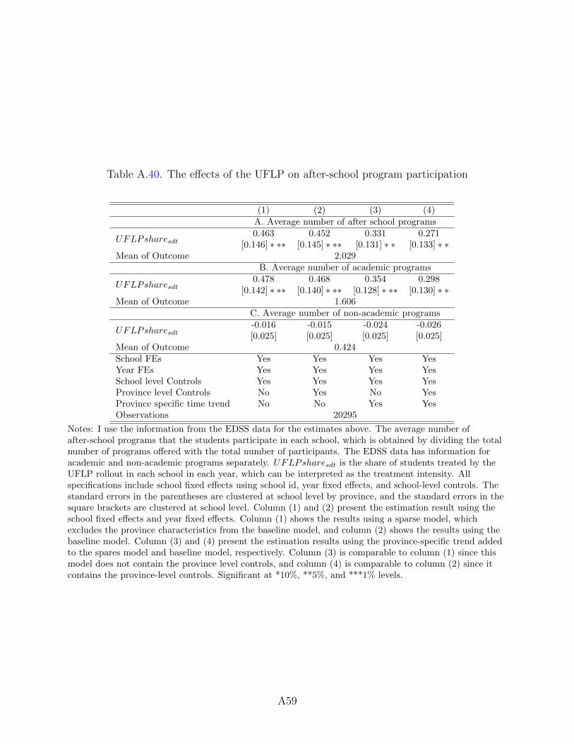
Table A.40. The effects of the UFLP on after-school program participation

(1) (2) (3) (4)

A. Average number of after school programs

UFLPsharesdt0.463

[0.146] ∗ ∗∗0.452

[0.145] ∗ ∗∗0.331

[0.131] ∗ ∗0.271

[0.133] ∗ ∗Mean of Outcome 2.029

B. Average number of academic programs

UFLPsharesdt0.478

[0.142] ∗ ∗∗0.468

[0.140] ∗ ∗∗0.354

[0.128] ∗ ∗∗0.298

[0.130] ∗ ∗Mean of Outcome 1.606

C. Average number of non-academic programs

UFLPsharesdt-0.016[0.025]

-0.015[0.025]

-0.024[0.025]

-0.026[0.025]

Mean of Outcome 0.424School FEs Yes Yes Yes YesYear FEs Yes Yes Yes YesSchool level Controls Yes Yes Yes YesProvince level Controls No Yes No YesProvince specific time trend No No Yes YesObservations 20295

Notes: I use the information from the EDSS data for the estimates above. The average number ofafter-school programs that the students participate in each school, which is obtained by dividing the totalnumber of programs offered with the total number of participants. The EDSS data has information foracademic and non-academic programs separately. UFLPsharesdt is the share of students treated by theUFLP rollout in each school in each year, which can be interpreted as the treatment intensity. Allspecifications include school fixed effects using school id, year fixed effects, and school-level controls. Thestandard errors in the parentheses are clustered at school level by province, and the standard errors in thesquare brackets are clustered at school level. Column (1) and (2) present the estimation result using theschool fixed effects and year fixed effects. Column (1) shows the results using a sparse model, whichexcludes the province characteristics from the baseline model, and column (2) shows the results using thebaseline model. Column (3) and (4) present the estimation results using the province-specific trend addedto the spares model and baseline model, respectively. Column (3) is comparable to column (1) since thismodel does not contain the province level controls, and column (4) is comparable to column (2) since itcontains the province-level controls. Significant at *10%, **5%, and ***1% levels.

A59

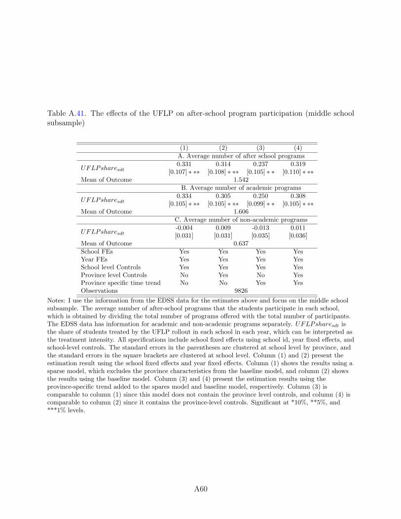
Table A.41. The effects of the UFLP on after-school program participation (middle schoolsubsample)

(1) (2) (3) (4)

A. Average number of after school programs

UFLPsharesdt0.331

[0.107] ∗ ∗∗0.314

[0.108] ∗ ∗∗0.237

[0.105] ∗ ∗0.319

[0.110] ∗ ∗∗Mean of Outcome 1.542

B. Average number of academic programs

UFLPsharesdt0.334

[0.105] ∗ ∗∗0.305

[0.105] ∗ ∗∗0.250

[0.099] ∗ ∗0.308

[0.105] ∗ ∗∗Mean of Outcome 1.606

C. Average number of non-academic programs

UFLPsharesdt-0.004[0.031]

0.009[0.031]

-0.013[0.035]

0.011[0.036]

Mean of Outcome 0.637School FEs Yes Yes Yes YesYear FEs Yes Yes Yes YesSchool level Controls Yes Yes Yes YesProvince level Controls No Yes No YesProvince specific time trend No No Yes YesObservations 9826

Notes: I use the information from the EDSS data for the estimates above and focus on the middle schoolsubsample. The average number of after-school programs that the students participate in each school,which is obtained by dividing the total number of programs offered with the total number of participants.The EDSS data has information for academic and non-academic programs separately. UFLPsharesdt isthe share of students treated by the UFLP rollout in each school in each year, which can be interpreted asthe treatment intensity. All specifications include school fixed effects using school id, year fixed effects, andschool-level controls. The standard errors in the parentheses are clustered at school level by province, andthe standard errors in the square brackets are clustered at school level. Column (1) and (2) present theestimation result using the school fixed effects and year fixed effects. Column (1) shows the results using asparse model, which excludes the province characteristics from the baseline model, and column (2) showsthe results using the baseline model. Column (3) and (4) present the estimation results using theprovince-specific trend added to the spares model and baseline model, respectively. Column (3) iscomparable to column (1) since this model does not contain the province level controls, and column (4) iscomparable to column (2) since it contains the province-level controls. Significant at *10%, **5%, and***1% levels.

A60

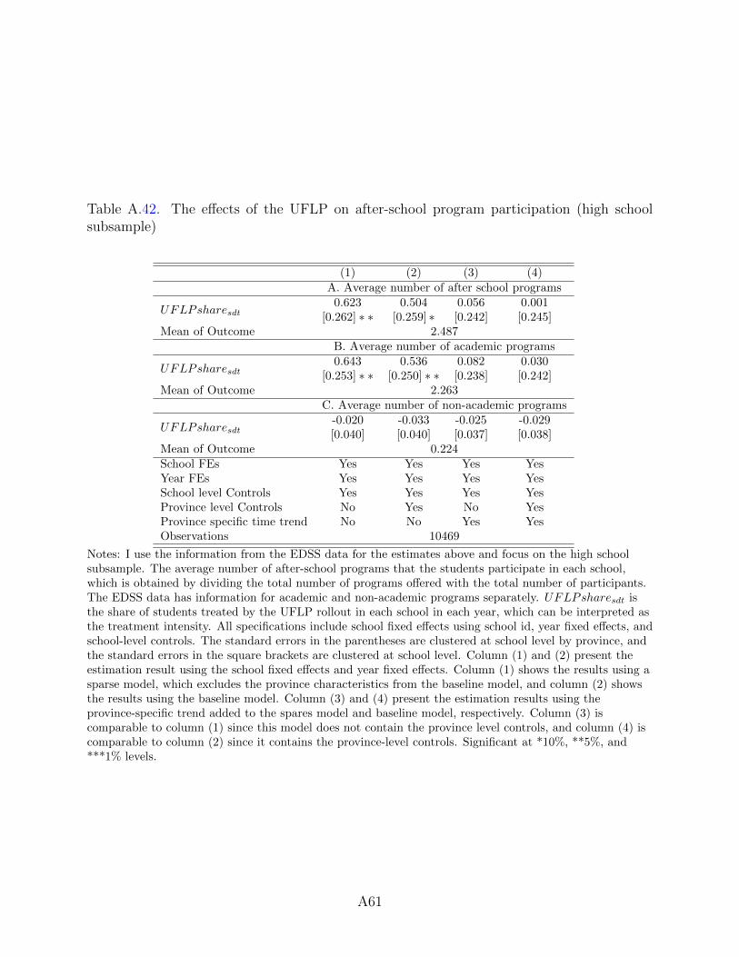
Table A.42. The effects of the UFLP on after-school program participation (high schoolsubsample)

(1) (2) (3) (4)

A. Average number of after school programs

UFLPsharesdt0.623

[0.262] ∗ ∗0.504

[0.259] ∗0.056

[0.242]0.001[0.245]

Mean of Outcome 2.487B. Average number of academic programs

UFLPsharesdt0.643

[0.253] ∗ ∗0.536

[0.250] ∗ ∗0.082

[0.238]0.030[0.242]

Mean of Outcome 2.263C. Average number of non-academic programs

UFLPsharesdt-0.020[0.040]

-0.033[0.040]

-0.025[0.037]

-0.029[0.038]

Mean of Outcome 0.224School FEs Yes Yes Yes YesYear FEs Yes Yes Yes YesSchool level Controls Yes Yes Yes YesProvince level Controls No Yes No YesProvince specific time trend No No Yes YesObservations 10469

Notes: I use the information from the EDSS data for the estimates above and focus on the high schoolsubsample. The average number of after-school programs that the students participate in each school,which is obtained by dividing the total number of programs offered with the total number of participants.The EDSS data has information for academic and non-academic programs separately. UFLPsharesdt isthe share of students treated by the UFLP rollout in each school in each year, which can be interpreted asthe treatment intensity. All specifications include school fixed effects using school id, year fixed effects, andschool-level controls. The standard errors in the parentheses are clustered at school level by province, andthe standard errors in the square brackets are clustered at school level. Column (1) and (2) present theestimation result using the school fixed effects and year fixed effects. Column (1) shows the results using asparse model, which excludes the province characteristics from the baseline model, and column (2) showsthe results using the baseline model. Column (3) and (4) present the estimation results using theprovince-specific trend added to the spares model and baseline model, respectively. Column (3) iscomparable to column (1) since this model does not contain the province level controls, and column (4) iscomparable to column (2) since it contains the province-level controls. Significant at *10%, **5%, and***1% levels.

A61

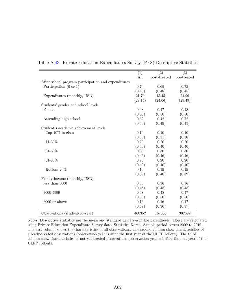
Table A.43. Private Education Expenditures Survey (PES) Descriptive Statistics

(1) (2) (3)All post-treated pre-treated

After school program participation and expendituresParticipation (0 or 1) 0.70 0.65 0.73

(0.46) (0.48) (0.45)Expenditures (monthly, USD) 21.70 15.45 24.96

(28.15) (24.06) (29.49)Students’ gender and school levels

Female 0.48 0.47 0.48(0.50) (0.50) (0.50)

Attending high school 0.62 0.42 0.72(0.49) (0.49) (0.45)

Student’s academic achievement levelsTop 10% in class 0.10 0.10 0.10

(0.30) (0.31) (0.30)11-30% 0.20 0.20 0.20

(0.40) (0.40) (0.40)31-60% 0.30 0.30 0.30

(0.46) (0.46) (0.46)61-80% 0.20 0.20 0.20

(0.40) (0.40) (0.40)Bottom 20% 0.19 0.19 0.19

(0.39) (0.40) (0.39)Family income (monthly, USD)

less than 3000 0.36 0.36 0.36(0.48) (0.48) (0.48)

3000-5999 0.48 0.48 0.47(0.50) (0.50) (0.50)

6000 or above 0.16 0.16 0.17(0.37) (0.36) (0.37)

Observations (student-by-year) 460352 157660 302692

Notes: Descriptive statistics are the mean and standard deviation in the parentheses. These are calculatedusing Private Education Expenditure Survey data, Statistics Korea. Sample period covers 2009 to 2016.The first column shows the characteristics of all observations. The second column show characteristics ofalready-treated observations (observation year is after the first year of the ULFP rollout). The thirdcolumn show characteristics of not-yet-treated observations (observation year is before the first year of theULFP rollout).

A62

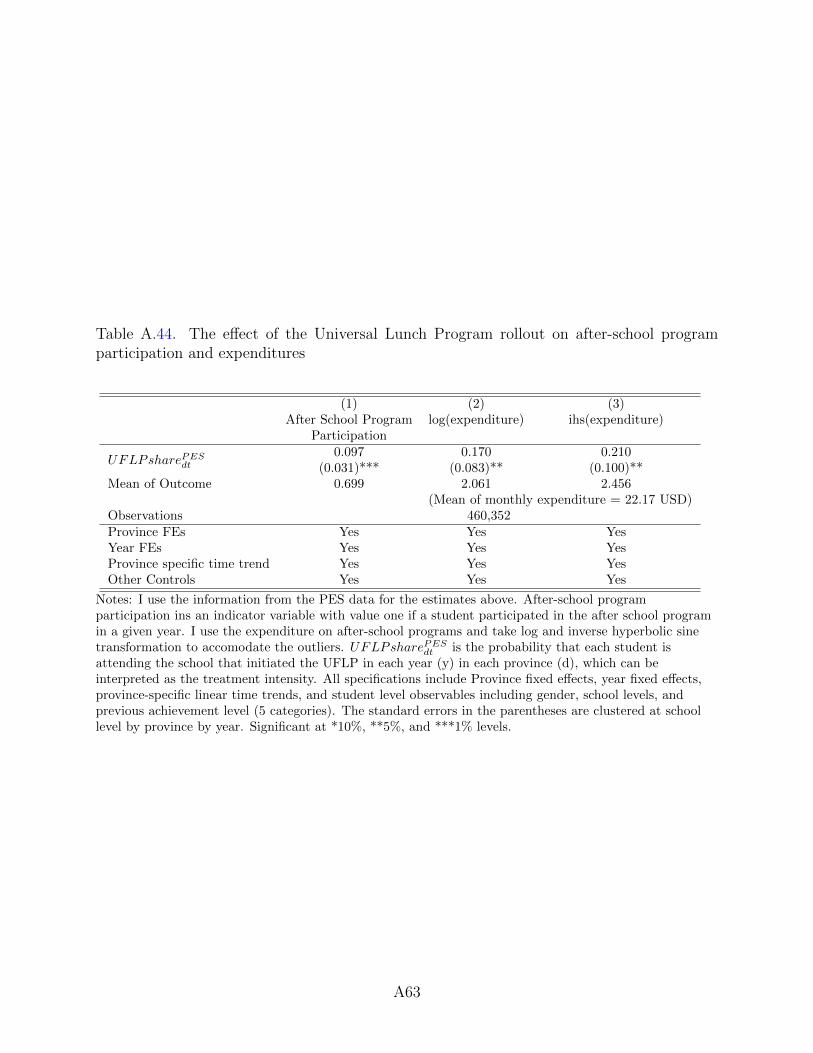
Table A.44. The effect of the Universal Lunch Program rollout on after-school programparticipation and expenditures

(1)After School Program

Participation

(2)log(expenditure)

(3)ihs(expenditure)

UFLPsharePESdt

0.097(0.031)***

0.170(0.083)**

0.210(0.100)**

Mean of Outcome 0.699 2.061 2.456(Mean of monthly expenditure = 22.17 USD)

Observations 460,352Province FEs Yes Yes YesYear FEs Yes Yes YesProvince specific time trend Yes Yes YesOther Controls Yes Yes Yes

Notes: I use the information from the PES data for the estimates above. After-school programparticipation ins an indicator variable with value one if a student participated in the after school programin a given year. I use the expenditure on after-school programs and take log and inverse hyperbolic sinetransformation to accomodate the outliers. UFLPsharePES

dt is the probability that each student isattending the school that initiated the UFLP in each year (y) in each province (d), which can beinterpreted as the treatment intensity. All specifications include Province fixed effects, year fixed effects,province-specific linear time trends, and student level observables including gender, school levels, andprevious achievement level (5 categories). The standard errors in the parentheses are clustered at schoollevel by province by year. Significant at *10%, **5%, and ***1% levels.

A63

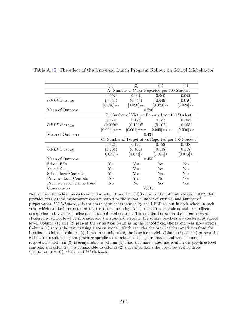
Table A.45. The effect of the Universal Lunch Program Rollout on School Misbehavior

(1) (2) (3) (4)

A. Number of Cases Reported per 100 Student

UFLPsharesdt

0.062(0.045)

[0.026] ∗∗

0.062(0.046)

[0.026] ∗∗

0.060(0.049)

[0.028] ∗∗

0.062(0.050)

[0.028] ∗∗Mean of Outcome 0.296

B. Number of Victims Reported per 100 Student

UFLPsharesdt

0.174(0.099)*

[0.064] ∗ ∗ ∗

0.175(0.100)*

[0.064] ∗ ∗ ∗

0.157(0.102)

[0.065] ∗ ∗ ∗

0.165(0.105)

[0.066] ∗∗Mean of Outcome 0.431

C. Number of Perpetrators Reported per 100 Student

UFLPsharesdt

0.126(0.106)[0.073] ∗

0.129(0.105)[0.073] ∗

0.123(0.118)[0.074] ∗

0.138(0.118)[0.075] ∗

Mean of Outcome 0.455School FEs Yes Yes Yes YesYear FEs Yes Yes Yes YesSchool level Controls Yes Yes Yes YesProvince level Controls No Yes No YesProvince specific time trend No No Yes YesObservations 20310

Notes: I use the school misbehavior information from the EDSS data for the estimates above. EDSS dataprovides yearly total misbehavior cases reported to the school, number of victims, and number ofperpetrators. UFLPsharesdt is the share of students treated by the UFLP rollout in each school in eachyear, which can be interpreted as the treatment intensity. All specifications include school fixed effectsusing school id, year fixed effects, and school-level controls. The standard errors in the parentheses areclustered at school level by province, and the standard errors in the square brackets are clustered at schoollevel. Column (1) and (2) present the estimation result using the school fixed effects and year fixed effects.Column (1) shows the results using a sparse model, which excludes the province characteristics from thebaseline model, and column (2) shows the results using the baseline model. Column (3) and (4) present theestimation results using the province-specific trend added to the spares model and baseline model,respectively. Column (3) is comparable to column (1) since this model does not contain the province levelcontrols, and column (4) is comparable to column (2) since it contains the province-level controls.Significant at *10%, **5%, and ***1% levels.

A64

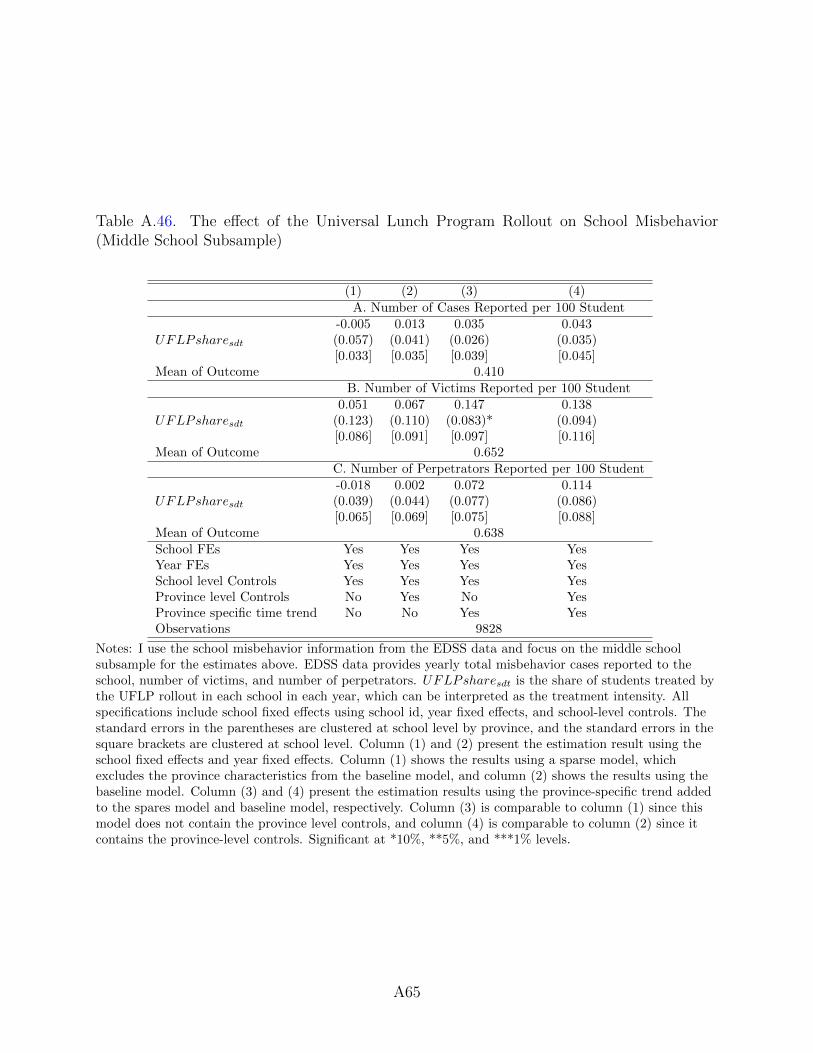
Table A.46. The effect of the Universal Lunch Program Rollout on School Misbehavior(Middle School Subsample)

(1) (2) (3) (4)

A. Number of Cases Reported per 100 Student

UFLPsharesdt

-0.005(0.057)[0.033]

0.013(0.041)[0.035]

0.035(0.026)[0.039]

0.043(0.035)[0.045]

Mean of Outcome 0.410B. Number of Victims Reported per 100 Student

UFLPsharesdt

0.051(0.123)[0.086]

0.067(0.110)[0.091]

0.147(0.083)*[0.097]

0.138(0.094)[0.116]

Mean of Outcome 0.652C. Number of Perpetrators Reported per 100 Student

UFLPsharesdt

-0.018(0.039)[0.065]

0.002(0.044)[0.069]

0.072(0.077)[0.075]

0.114(0.086)[0.088]

Mean of Outcome 0.638School FEs Yes Yes Yes YesYear FEs Yes Yes Yes YesSchool level Controls Yes Yes Yes YesProvince level Controls No Yes No YesProvince specific time trend No No Yes YesObservations 9828

Notes: I use the school misbehavior information from the EDSS data and focus on the middle schoolsubsample for the estimates above. EDSS data provides yearly total misbehavior cases reported to theschool, number of victims, and number of perpetrators. UFLPsharesdt is the share of students treated bythe UFLP rollout in each school in each year, which can be interpreted as the treatment intensity. Allspecifications include school fixed effects using school id, year fixed effects, and school-level controls. Thestandard errors in the parentheses are clustered at school level by province, and the standard errors in thesquare brackets are clustered at school level. Column (1) and (2) present the estimation result using theschool fixed effects and year fixed effects. Column (1) shows the results using a sparse model, whichexcludes the province characteristics from the baseline model, and column (2) shows the results using thebaseline model. Column (3) and (4) present the estimation results using the province-specific trend addedto the spares model and baseline model, respectively. Column (3) is comparable to column (1) since thismodel does not contain the province level controls, and column (4) is comparable to column (2) since itcontains the province-level controls. Significant at *10%, **5%, and ***1% levels.

A65

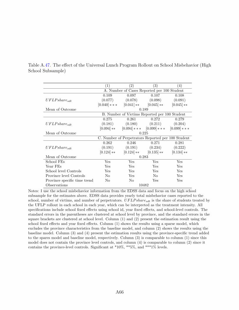
Table A.47. The effect of the Universal Lunch Program Rollout on School Misbehavior (HighSchool Subsample)

(1) (2) (3) (4)

A. Number of Cases Reported per 100 Student

UFLPsharesdt

0.109(0.077)

[0.040] ∗ ∗ ∗

0.097(0.078)

[0.041] ∗∗

0.107(0.098)

[0.045] ∗∗

0.108(0.091)

[0.045] ∗∗Mean of Outcome 0.189

B. Number of Victims Reported per 100 Student

UFLPsharesdt

0.275(0.181)

[0.094] ∗∗

0.261(0.180)

[0.094] ∗ ∗ ∗

0.272(0.211)

[0.099] ∗ ∗ ∗

0.279(0.204)

[0.099] ∗ ∗ ∗Mean of Outcome 0.225

C. Number of Perpetrators Reported per 100 Student

UFLPsharesdt

0.262(0.191)

[0.124] ∗∗

0.246(0.191)

[0.124] ∗∗

0.271(0.234)

[0.135] ∗∗

0.281(0.222)

[0.134] ∗∗Mean of Outcome 0.283School FEs Yes Yes Yes YesYear FEs Yes Yes Yes YesSchool level Controls Yes Yes Yes YesProvince level Controls No Yes No YesProvince specific time trend No No Yes YesObservations 10482

Notes: I use the school misbehavior information from the EDSS data and focus on the high schoolsubsample for the estimates above. EDSS data provides yearly total misbehavior cases reported to theschool, number of victims, and number of perpetrators. UFLPsharesdt is the share of students treated bythe UFLP rollout in each school in each year, which can be interpreted as the treatment intensity. Allspecifications include school fixed effects using school id, year fixed effects, and school-level controls. Thestandard errors in the parentheses are clustered at school level by province, and the standard errors in thesquare brackets are clustered at school level. Column (1) and (2) present the estimation result using theschool fixed effects and year fixed effects. Column (1) shows the results using a sparse model, whichexcludes the province characteristics from the baseline model, and column (2) shows the results using thebaseline model. Column (3) and (4) present the estimation results using the province-specific trend addedto the spares model and baseline model, respectively. Column (3) is comparable to column (1) since thismodel does not contain the province level controls, and column (4) is comparable to column (2) since itcontains the province-level controls. Significant at *10%, **5%, and ***1% levels.

A66