THE ECOLOGY OF LAKES AND RIVERS IN THE SOUTHERN BOREAL SHIELD:

WATER QUALITY, COMMUNITY STRUCTURE, AND CUMULATIVE EFFECTS

by

Fredric Christopher Jones

A thesis submitted in partial fullfillment of the requirements for the degree of

doctor of philosophy (PhD) in Boreal Ecology

Faculty of Graduate Studies, Laurentian University,

Sudbury, Ontario

© Fredric Christopher Jones, 2018

ii

THESIS DEFENCE COMMITTEE/COMITÉ DE SOUTENANCE DE THÈSE

Laurentian Université/Université Laurentienne

Faculty of Graduate Studies/Faculté des études supérieures

Title of Thesis

Titre de la thèse THE ECOLOGY OF LAKES AND RIVERS IN THE SOUTHERN BOREAL

SHIELD: WATER QUALITY, COMMUNITY STRUCTURE, AND

CUMULATIVE EFFECTS

Name of Candidate

Nom du candidat Jones, Fredric Christopher

Degree

Diplôme Doctor of Philosophy

Department/Program Date of Defence

Département/Programme Boreal Ecology Date de la soutenance June 07, 2018

APPROVED/APPROUVÉ

Thesis Examiners/Examinateurs de thèse:

Dr. John Gunn

(Co-Supervisor/Co-directeur de thèse)

Dr. Brie Edwards

(Co-Supervisor/Co-directrice de thèse)

Dr. John Bailey

(Committee member/Membre du comité)

Dr. Richard Johnson

(Committee member/Membre du comité)

Approved for the Faculty of Graduate Studies

Approuvé pour la Faculté des études supérieures

Dr. David Lesbarrères

Monsieur David Lesbarrères

Dr. Garry Scrimgeour Dean, Faculty of Graduate Studies

(External Examiner/Examinateur externe) Doyen, Faculté des études supérieures

Dr. Yves Alaire

(Internal Examiner/Examinateur interne)

ACCESSIBILITY CLAUSE AND PERMISSION TO USE

I, Fredric Christopher Jones, hereby grant to Laurentian University and/or its agents the non-exclusive license to

archive and make accessible my thesis, dissertation, or project report in whole or in part in all forms of media, now

or for the duration of my copyright ownership. I retain all other ownership rights to the copyright of the thesis,

dissertation or project report. I also reserve the right to use in future works (such as articles or books) all or part of

this thesis, dissertation, or project report. I further agree that permission for copying of this thesis in any manner, in

whole or in part, for scholarly purposes may be granted by the professor or professors who supervised my thesis

work or, in their absence, by the Head of the Department in which my thesis work was done. It is understood that

any copying or publication or use of this thesis or parts thereof for financial gain shall not be allowed without my

written permission. It is also understood that this copy is being made available in this form by the authority of the

copyright owner solely for the purpose of private study and research and may not be copied or reproduced except as

permitted by the copyright laws without written authority from the copyright owner.

iii

ABSTRACT

Cumulative effects are the collective ecological effects of multiple human

activities. Cumulative effects assessment (CEA) is concerned with quantifying effects of

natural environmental factors and human activities. CEA has not lived up to its promise

as a precautionary instrument for sustainability, in part because our knowledge of

stressors and their effects is elementary; monitoring systems (needed to characterize

ecological condition and how it changes over time) are insufficient; and numerical

methods for associating stressors and effects, and for forecasting development

outcomes, are lacking.

This thesis reviews the environmental appraisal literature to synthesize CEA’s

theoretical underpinnings, articulate its impediments, and establish that ecological

monitoring and modelling activities are critical to success. Three research chapters

overcome several scientific barriers to effective CEA. Data from spatial and temporal

surveys of lake and stream water chemistry and benthic community structure are used

to evaluate candidate monitoring indicators, identify minimally impacted reference

waterbodies, characterize baseline water quality and biological condition, and quantify

cumulative effects of land use and natural environmental variation (spatial survey: 107

lakes and 112 streams sampled in 2012 or 2013; temporal survey: 19 lakes sampled

between 1993 and 2016).

The research was conducted in Canada’s Muskoka River Watershed, a 5660 km2

area of Precambrian Shield that drains to Lake Huron. This area’s combination of

extensive remaining natural areas and pervasive human influence makes it ideal for

studying cumulative effects. It is also characterized by many lakes and their connecting

stream and river channels, which integrate effects of stressors in their catchments and

constitute logical focal points for CEA. Moreover, the local planning authority (District

iv

Municipality of Muskoka) is striving to implement CEA and establish a cumulative

effects monitoring program centered on water as its foremost resource; therefore,

practical applications of the research have, been identified.

Universal numerical methods, which are transferrable to other study areas, are

used. Random forest models (an extension of the algorithm used to produce

classification or regression trees) are shown to model the singular and collective effects

of land-use and natural factors on water chemistry and benthic community structure,

and to quantify the sensitivities, and identify the important drivers of various chemical

and biological indicators of aquatic ecosystem condition. Partial dependencies from the

random forests (i.e., the mean predicted values of a given indicator that occurred across

the observed range of a selected predictor) are paired with TITAN (Threshold Indicator

Taxa Analysis) to investigate biological and chemical “onset-of-effect” thresholds along

gradients of human development. Declining calcium concentrations and amphipod

abundances are demonstrated in lakes, and generalized linear models forecast an

average 57% decrease in the abundances of these animals to occur by the time lake-

water calcium concentrations reach expected minima.

As its key findings, the thesis highlights sensitive indicators that should be

included in a cumulative effects monitoring program, and are to be preferred when

forecasting outcomes of changed land-use or environmental attributes. Empirical break-

points, where effects of stressor exposures become detectable, are also identified.

These thresholds can be used to distinguish reference and impacted conditions, so that

normal indicator ranges and associated assessment criteria (important CEA precursors)

can be objectively derived. In addition, the potential severity of cumulative effects is

exemplified by marked declines in the abundances of lake dwelling amphipods, which

could propagate through food webs to substantially alter soft-water Boreal ecosystems.

v

ACKNOWLEDGEMENTS

I thank my academic supervisor, John Gunn, co-supervisors, John Bailey and Brie

Edwards, and graduate committee members, Richard Johnson and Simon Linke, for

their guidance. I’m grateful to Ontario’s Ministry of Environment and Climate Change

and the Canadian Water Network for funding this project. Thanks to Keith Somers,

Melissa Robillard, and Rachael Fletcher for seeing the value of this project and allowing

me some flexibility in my work schedule to undertake the research. I acknowledge Keith

Somers, Jim Rusak, Simon Courtenay, and Jan Ciborowski for sharing their ideas, and

providing encouragement. Thanks also to Sarah Sinclair and several other technicians

who assisted with stream and lake sampling, and sample processing activities. I

acknowledge my long-suffering family and friends for tolerating me and this project.

1

TABLE OF CONTENTS

ABSTRACT…………………………………………………………………………… iii

ACKNOWLEDGEMENTS ………………………………………………………….. v

TABLE OF CONTENTS ………………………………………………………….… 1

PART 1: INTRODUCTION …………………………………………………………. 2

PART 2: CUMULATIVE EFFECTS ASSESSMENT ― THEORETICAL

UNDERPINNINGS AND BIG PROBLEMS ……………………………………….

24

PART 3: RANDOM FORESTS AS CUMULATIVE EFFECTS MODELS ― A

CASE STUDY OF LAKES AND RIVERS IN MUSKOKA CANADA ……………

43

PART 4: ONSET-OF-EFFECT THRESHOLDS AND REFERENCE

CONDITIONS ― A CASE STUDY OF THE MUSKOKA RIVER

WATERSHED, CANADA…………………………………………………………....

62

PART 5: DECLINING AMPHIPOD ABUNDANCE IS LINKED TO LOW AND

DECLINING CALCIUM CONCENTRATIONS IN LAKES OF THE SOUTH

PRECAMBRIAN SHIELD …………………………………………………………...

104

PART 6: SUMMARY, CONCLUSIONS AND DISCUSSION ..………………….. 143

2

Part 1: INTRODUCTION

3

Background

As the branch of biology that deals with interactions of organisms with one

another, and with their physical environment, Ecology’s fundamental goal is to explain

and predict the occurrences and abundances of taxa (Townsend 1989, Belovsky et al.

2004, Temperton and Hobbs 2004). Its sub-discipline, Community Ecology, is

concerned with explaining the distributions, abundances, and interactions of taxa

(Liebold et al. 2004) that co-occur as assemblages at different places or times.

Community assembly refers to the processes by which communities arise.

Current paradigms emphasize dispersal, niche limitation (taxa not capable of tolerating

the physical conditions present at a given location being excluded from that location),

biotic interactions (e.g., predation, competition), evolution, and neutral (random)

processes of extirpation and colonization as most important (Belyea and Lancaster

1999, Hubbell 2001, Fussmann et al. 2007)1.

Stressor exposures and natural disturbances are universal determinants of the

taxonomic structure and functions of ecosystems (Hutchinson 1957). The term

ecological effect describes a change to the structure or function of the ecosystem — an

alteration of habitat, biota, or (and) their interactions. Such changes are typically

measured against the normal range of variability associated with a specified spatial or

temporal baseline (Kilgour et al. 1998). Effects can accumulate via repeated insults of a

single stressor, or via the interaction of multiple stressors.

1 These processes are arranged in a visually intuitive way in the Ecological Filters metaphor of community

assembly, in which community assembly is viewed as a series of filters or sieves through which the regional pool of taxa must pass to determine community composition at any place or time (Mueller-Dombois and Ellenberg 1974, Van der Walk 1981, Drake 1990, Poff 1997, and Patrick and Swan 2011).

4

Stressor exposures, the type and intensity of disturbances, and the magnitude of

the resulting ecological responses generally depend on one’s reference point2 (Belyea

and Lancaster 1999, Weiher et al. 2011), and can vary spatially and temporally (Sousa

1980, 1984; Resh et al. 1988; Miller et al. 2011). Such complexity makes it difficult to

understand and predict ecological effects (Lamothe et al. 2018). Indeed, our present

ecological theories, concepts, and paradigms lack predictive power as a rule (Peters

1991, Keddy 1992a and 1992b), which is problematic because, “as ecology matures

and as the world’s environmental problems continue to multiply, the need for general

predictive models also grows” (Shapiro 1993). Quantitative and predictive models of

community assembly would lend themselves to scientific testing, and would have many

deployments against the World’s problems — application in environmental appraisal

being an obvious example.

The worldwide process of environmental impact assessment was borne out of

the 1969 US National Environmental Policy Act (Benson 2003, Pope et al. 2013), as a

way to identify, predict, evaluate and mitigate the effects of development projects

(Glasson et al. 2013). Scrutiny of the process has demonstrated that environmental

impact assessment remains a young and unproven field (Bérubé 2007) in which

cumulative effects, the combined effects of multiple human activities (Scherer 2011),

have not been adequately considered (Damman et al. 1995, Duinker and Greig 2006,

Gunn and Noble 2011).

Cumulative effects assessment (CEA) is both an applied science (Cashmore

2004), and a sub-discipline of environmental impact assessment (Morrison-Saunders et

2 Scale is critically important because our ability to understand local and regional community assembly

depends on the spatial scale at which communities are defined and the scale at which assembly processes operate (Weiher et al. 2011).

5

al. 2014). It was proposed as a way to evaluate the collective environmental effects of

human actions (Dubé 2003, Seitz et al. 2011); however, its theoretical underpinnings

have not been fully articulated, so it remains unclear precisely what CEA is supposed to

achieve (Cashmore 2004, Judd et al. 2015). For this reason, agreement between its

theory and practice has not been assessed (Lawrence 2000, Pope et al. 2013), and

many signals of the deepening unsustainability of human enterprise — the remarkable

transformation of Earth’s surface, anthropogenic increases of atmospheric CO2

concentrations, hijacking of the World’s nitrogen cycle, excessive use and alteration of

fresh water, and extinctions of numerous species (Vitousek et al. 1997, Foley et al.

2005, Steffen et al. 2007) —suggest it has been ineffectual as a precautionary

sustainability strategy.

Because of different legislative and regulatory contexts, there is regional variation

in the way CEA is practiced; however, it usually proceeds via the following six steps: (1)

valued ecosystem components are identified to focus the appraisal on a small number

of important ecosystem features (Canter and Atkinson 2011); (2) the physical and

temporal boundaries of the appraisal are set; (3) activities capable of affecting valued

ecosystem components are identified; (4) baseline condition is characterized using

appropriate indicators; (5) cumulative effects of identified activities are modeled (and the

significance of predicted effects is assessed); and (6) environmental monitoring is

conducted to track realized outcomes and evaluate performance of the appraisal

process (Damman et al. 1995; Ross 1998; Canter and Ross 2010; Connelly 2011; Seitz

et al. 2011)

6

The inherent unpredictability of ecosystems and ecological effects makes

uncertainty an unavoidable part of CEA (Chapman and Maher 2014). Monitoring is

fundamental as a tool for mitigating the risks of uncertainty, because it indicates

ecosystem form and function, allows the condition and variability of valued ecosystem

components to be quantified (Ball et al. 2013), signals when conditions are changing

(Cairns et al. 1993), and provides datasets that can be modeled to associate stressors

with their ecological outcomes (e.g., Therivel and Ross 2007; Schultz 2012).

Biological (effect-based) and chemical (stressor based) indicators have

complementary roles in CEA. Stressor-based indicators describe physico-chemical

conditions and quantify stressor exposures (Roux et al. 1999). Biological indicators

“integrate a cumulative response to environmental stress” (Munkittrick et al. 2000; Dubé

2003) by measuring ecosystem structure or function. Such indicators should be

conceptually simple (so their meanings can be conveyed to diverse audiences),

predictive, sensitive (to human and environmental factors relevant to CEA), precise

enough that they can discriminate stressor-specific effects, and should have reasonable

sampling and data requirements that make them economically feasible (Cairns et al.

1993; Niemi and McDonald 2004; Bonada et al. 2006).

CEA requires the effects of multiple stressors to be quantified, both singly and in

combination (Judd et al. 2015). Descriptive or predictive models are vital tools for

describing stressor effects, guiding the design of monitoring schemes, and predicting

outcomes of alternative scenarios of human activity (Rubin and Kaivo-Oja 1999, Seitz et

al. 2013, Russell-Smith et al. 2015).

7

Water is essential for life. For this reason, the ecosystem is commonly viewed as

the primary user of water (Participants of Muskoka Summit for the Environment 2010),

and access to sufficient clean water is commonly viewed as a human right (Gupta et al.

2010). Surface waterbodies, including lakes and rivers, are tightly coupled with

chemical, physical, and biological processes that play out in their catchments (Hynes

1970, Wetzel 2001). They are exposed to (Nõges et al., 2016), and subsequently

integrate effects of, a multitude of stressors (Lowell et al., 2000, Townsend et al., 2008,

Ormerod et al. 2010, Jackson et al. 2016), which makes them some of the most

threatened ecosystems on Earth (Schindler 2001, Carpenter et al. 2011) and a critical

consideration for CEA. The Boreal region is well suited to research on cumulative

effects (e.g., Sorensen et al. 2008, Houle et al. 2010) and cumulative effects

assessment (e.g., Dubé et al. 2006, Seitz et al. 2011) because it contains many

thousands of lakes, and is important globally as a vast relatively natural ecosystem,

and as a source of timber, energy, minerals, and other natural resources (Luke et al

2007).

I selected a case-study boreal watershed, the Muskoka River Watershed, where I

conducted a spatial survey of littoral benthic macroinvertebrate communities and water

chemistry in 107 lakes and 112 rivers, and where a temporal survey of the same

biological and chemical attributes had been underway since 1993. I selected the

Muskoka River Watershed for several reasons: (1) Its gradients of geology, hydrology,

and land-use provide variation that could be exploited to model community structure,

community thresholds, and cumulative effects of multiple environmental factors. (2) The

watershed has significant development, agriculture, and forestry — human activities

8

known to alter a variety of physical, chemical, and biological properties of waterbodies,

(Utz et al. 2009) — but is also rare in southern Canada for having a large number of

lakes and streams that have no measurable development in their catchments, and are

exposed only to atmospheric pollution, making them suitable for exploring minimally

impacted (sensu Stoddard et al. 2006) reference conditions. (3) The watershed’s lakes

and rivers are changing physically, chemically and biologically — for example, air

temperatures are rising and wind speeds are decreasing, which has led to phenological

changes to lake ice cover and lake thermal stratification (Yao et al. 2013, Palmer et al.

2014); conductivity and the concentrations of calcium, phosphorus, and various metals

are declining, while pH, and the concentrations of dissolved organic carbon, nitrogen,

and chloride are increasing (Jeziorski et al. 2008, Eimers et al. 2009; Palmer et al.

2011); and many lakes have been invaded by the spiny water flea, which has resulted

in reduced pelagic biodiversity (Yan et al. 2011). (4) Multiple ecological stressors are

implicated in many of these changes (e.g., Watmough and Aherne 2008, Yao et al.

2013), which provides a suitable backdrop for cumulative effects research; and (5) one

of Canada’s primary urban and economic centres, the Greater Toronto Area (located

within a 2-hour drive to the south) exerts considerable development pressure on the

Watershed, makes the management of cumulative effects a fundamental concern, and

suggests a variety of practical applications for research designed to monitor and model

cumulative effects (Eimers 2016).

9

Problem Statement

Several challenges related to monitoring and modeling cumulative effects need

to be overcome in order for cumulative effects assessment to be undertaken in boreal

watersheds.

Our knowledge about stressors and effects on most ecosystems, including boreal

lakes and streams, is rudimentary (Venier et al 2014). Integrating the information that

does exist is problematic because cumulative effects assessment lacks straightforward

and effective methods for associating stressors and effects, and for exploring the

outcomes of development scenarios. Models capable of handling stressor interactions

and non-linear responses are needed (Ball et al. 2013).

Great interest in monitoring cumulative effects has been generated in some

locations (e.g., Eimers 2016), but robust monitoring systems generally don’t exist (Ball

et al. 2013, Dubé et al. 2013, Venier et al. 2014). Ecological condition can only be

assessed relative to reference benchmarks and the normal range of natural variation

(Kilgour et al. 1998, Hawkins et al. 2010, Mitchell et al. 2014, Clapcott et al. 2017), but

chemical and biological reference conditions are not well understood for many areas,

including Muskoka. Quantitative criteria based on measured exposures to stress are

generally used to define what qualifies as a reference site; however, objective criteria

for determining the level of stressor exposure that is acceptable are lacking3.

From a theoretical perspective, the long-term stability of ecosystems suggests

some capacity to resist disturbance; however, as human impacts or fluctuations in

3In fact, subjective judgement is the norm at multiple junctures in the process of ecological assessment,

including the definition and selection of reference sites, selection of metrics and numerical methods for evaluating index performance (Feio et al 2016).

10

natural factors become extreme, a threshold may be reached where normal processes

of community assembly are overridden and effects become apparent (Pardo et al. 2012,

Roubeix et al. 2016). Such onset-of-effect thresholds have been hypothesized

(Hilderbrand et al. 2010, Pardo et al. 2012), and could be used to objectively delineate

the least-disturbed reference condition (Ciborowski et al. 2015), but there is little

empirical evidence to support their existence (Pardo et al. 2012).

Chemical or biological condition is often summarized with indicator metrics but,

for many Boreal areas, little information is available to describe how sensitive candidate

indicators are to various natural environmental features and human stressors. So many

questions remain about their accuracy and bias (i.e., how influenced they are by natural

factors, and therefore what variables should be considered when matching reference

sites and test sites; Hawkins et al. 2010), precision (i.e., how similar their scores are

when measured in similar contexts), responsiveness (i.e., how predictably their scores

change in response to stressor exposures), and sensitivity (i.e., how closely high and

low scores correspond with high and low stressor exposures; Mazor et al. 2016).

Perhaps the most critical questions for CEA pertain to how accurately metric values can

be predicted, and how well suited they are for use in “futuring” analyses4 (Therivel and

Ross 2007; Canter and Atkinson 2011).

As an example of multiple environmental stressors and cumulative effects,

declining calcium concentrations have been documented in many lakes in the southern

Boreal Shield (Watmough and Aherne 2008, Jeziorski et al. 2008). Low calcium

concentrations represent a stressor for Calcium-rich taxa, and (particularly when

4 i.e., analyses undertaken to explore the range of outcomes possible from alternative scenarios of human

activity

11

combined with other climate and development-related changes) cumulative effects on

aquatic communities are possible (Jeziorski and Smol 2016). Declines of crayfish

abundances (Edwards et al. 2009, Edwards et al. 2013, Hadley et al. 2015) and altered

species composition of zooplankton communities (Jeziorski et al. 2008, Shapiera et al.

2012) have been demonstrated, but effects on amphipods (an abundant component of

the benthic taxa that has high Ca demands) have not been investigated despite their

potential to have important ecological consequences.

Research Objectives

This thesis begins with a philosophical chapter that synthesizes the theory

behind cumulative effects assessment (Chapter 2 — Cumulative Effects Assessment:

Theoretical Underpinnings and Big Problems). By way of a critical review, it clarifies

societal aspirations for CEA, assesses agreement between its theory and practice, and

articulates its foremost challenges and opportunities. Notable shortcomings associated

with describing, predicting, and monitoring cumulative effects are addressed in three

subsequent research chapters.

Chapter 3 (Random Forests as Cumulative Effects Models: A Case Study of

Lakes and Rivers in Muskoka Canada) models cumulative effects and evaluates several

candidate monitoring indicators using lake and river water chemistry and benthic-

invertebrate community data from the case-study watershed in order to answer the

following four questions: (1) which measures of lake and river water chemistry and

benthic community structure can be modeled and predicted most accurately, and

therefore show the most promise as cumulative effects indicators? (2) What are the

12

combined and singular effects of human activities (e.g., urbanization, agriculture),

hydrologic, physiographic, and morphometric factors on these indicators? (3) Can any

chemical or biological attributes of lakes or rivers be predicted accurately enough, and

are these models sensitive enough to land-use changes, to be used in scenario models

that explore potential ecological consequences of increased development?

In this chapter, I propose that the suitability of any given candidate CEA indicator

can be assessed according to how precisely and accurately it can be predicted from

natural environmental features and how sensitively it responds to measures of human

activities, and I demonstrate how random forests5 (Breiman 2001) can be used to make

these assessments and predict outcomes of alternative scenarios of human activity.

An approach for objectively distinguishing reference and impacted conditions is

presented in Chapter 4 (Onset-of-effect Thresholds and Reference Conditions: A Case

Study of the Muskoka River Watershed, Canada). In this paper, 107 lakes and 112

streams are classified as reference or impacted. According to the concept of minimal

disturbance (Stoddard et al. 2006), sites having no exposures to land-use stress are

designated as reference, and lakes or streams having measurable road density,

urbanization, or agriculture in their catchments are considered impacted. Two

complementary statistical methods (partial dependence plots from random forest

models and TITAN [threshold indicator taxa analysis]) are then used to investigate the

existence of chemical and biological onset-of-effect thresholds along stressor gradients.

Where present, these thresholds — i.e., break-points where stressors begin to override

5 Random forests are ensembles of classification or regression trees. They make no assumptions about

the distributions of predictor or response variables. They can be used to assess datasets having a large ratio of predictors to observations. They can incorporate complex predictor interactions, without these interactions having to be pre-specified; and they can account for multicollinearity of predictors, and non-linear relationships between predictors and the response variable (Jones and Linder 2015).

13

natural processes such that effects become detectable — are used to make empirical

adjustments to the criteria used to distinguish reference and impacted waterbodies.

Normal reference ranges and typical impacted ranges of benthic community structure

and water chemistry are then tabulated as critical percentiles and tolerance regions, the

degree of interspersion of reference and impacted sites is assessed, and cumulative

effects of land-use stress are described as spatial patterns of biological and chemical

variation.

Chapter 5 (Declining Amphipod Abundance is Linked to Low and Declining

Calcium Concentrations in Lakes of the south Precambrian Shield) investigates the

biological effects of Ca decline (an emerging stressor in several parts of the Boreal

where historical acid deposition, logging, and development has altered Ca weathering

rates; Watmough and Aherne 2008) on amphipod abundances using data from the

spatial survey of lakes described in Chapters 3 and 4, and also from a series of 19 long-

term study lakes that were sampled between 1993 and 2016. From a spatial

perspective, the study investigates whether amphipods (a crustacean with high calcium

demands, relative to many other aquatic taxa; Cairns and Yan 2009) are more likely to

be found in high-Ca lakes than in low-Ca lakes; whether there is a low-level Ca

threshold, below which amphipods are unable to persist in lakes; and how important Ca

is as a predictor of amphipod abundance, relative to the importance of other chemical,

morphometric, or physical-habitat factors? From a temporal perspective, the study

quantifies declines in amphipod abundance that have occurred over the last 23 years;

assesses how important a role Ca has had in these declines, and forecasts how

14

abundant amphipods will be in the future if calcium levels continue to fall, as predicted

by several authors (e.g., Watmough and Aherne 2008).

15

References Ball, M., Somers, G., Wilson, J. E., Tanna, R., Chung, C., Duro, D. C., & Seitz, N.

(2013). Scale, assessment components, and reference conditions: issues for

cumulative effects assessment in Canadian watersheds. Integrated environmental

assessment and management, 9(3), 370-379.

Belovski, G.E., D.B. Botkin, T.A. Crowl, K.W. Cummins, J.F. Franklin, M.L. Hunter, A.

Joern, D.B. Lindenmayer, J.A. MacMahon, C.R. Margules, and J.M. Scott. 2004.

Ten suggestions to strengthen the science of ecology. BioScience 54(4): 345-351.

Belyea, L.R., and J. Lancaster. 1999. Assembly rules within a contingent ecology. Oikos

86: 402-416.

Benson, J. F. (2003). What is the alternative? Impact assessment tools and sustainable

planning. Impact Assessment and Project Appraisal, 21(4), 261-280.

Bérubé, M. (2007). Cumulative effects assessments at Hydro-Québec: what have we

learned?. Impact assessment and project appraisal, 25(2), 101-109.

Bonada, N., Prat, N., Resh, V. H., & Statzner, B. (2006). Developments in aquatic insect

biomonitoring: a comparative analysis of recent approaches. Annu. Rev. Entomol.,

51, 495-523.

Breiman, L. (2001). Random forests. Machine learning, 45(1), 5-32.

Cairns, J., McCormick, P. V., & Niederlehner, B. R. (1993). A proposed framework for

developing indicators of ecosystem health. Hydrobiologia, 263(1), 1-44.

Cairns, A., & Yan, N. (2009). A review of the influence of low ambient calcium

concentrations on freshwater daphniids, gammarids, and crayfish. Environmental

Reviews, 17: 67-79.

Canter, L. W., & Atkinson, S. F. (2011). Multiple uses of indicators and indices in

cumulative effects assessment and management. Environmental Impact

Assessment Review, 31(5), 491-501.

Canter, L., & Ross, B. (2010). State of practice of cumulative effects assessment and

management: the good, the bad and the ugly. Impact Assessment and Project

Appraisal, 28(4), 261-268.

Carpenter, S. R., Stanley, E. H., & Vander Zanden, M. J. (2011). State of the world's

freshwater ecosystems: physical, chemical, and biological changes. Annual review

of Environment and Resources, 36, 75-99.

16

Cashmore, M. (2004). The role of science in environmental impact assessment: process

and procedure versus purpose in the development of theory. Environmental

Impact Assessment Review, 24(4), 403-426.

Chapman, P. M., & Maher, B. (2014). The need for truly integrated environmental

assessments. Integrated environmental assessment and management, 10(2), 151-

151.

Ciborowski, J., Kovalenko, K., Host, G., Howe, R. W., Reavie, E., Brown, T. N., ... &

Johnson, L. B. (2015). Developing Great Lakes Bioindicators of Environmental

Condition and Recovery from Degradation with Reference to Watershed-based

Risk of Stress.

Clapcott, J. E., Goodwin, E. O., Snelder, T. H., Collier, K. J., Neale, M. W., & Greenfield,

S. (2017). Finding reference: a comparison of modelling approaches for predicting

macroinvertebrate community index benchmarks. New Zealand Journal of Marine

and Freshwater Research, 51(1), 44-59.

Connelly, R. B. (2011). Canadian and international EIA frameworks as they apply to

cumulative effects. Environmental Impact Assessment Review, 31(5), 453-456.

Cutler, D. R., Edwards, T. C., Beard, K. H., Cutler, A., Hess, K. T., Gibson, J., & Lawler,

J. J. (2007). Random forests for classification in ecology. Ecology, 88(11), 2783-

2792.

Damman, D. C., Cressman, D. R., & Sadar, M. H. (1995). Cumulative effects

assessment: the development of practical frameworks. Impact Assessment, 13(4),

433-454.

Drake, J.A. 1990. The mechanics of community assembly and succession. Journal of

Theoretical Biology 147: 213-233.

Dubé, M. G. (2003). Cumulative effect assessment in Canada: a regional framework for

aquatic ecosystems. Environmental impact assessment review, 23(6), 723-745.

Dubé, M., Johnson, B., Dunn, G., Culp, J., Cash, K., Munkittrick, K., ... & Resler, O.

(2006). Development of a new approach to cumulative effects assessment: a

northern river ecosystem example. Environmental monitoring and assessment,

113(1-3), 87-115.

Dubé, M. G., Duinker, P., Greig, L., Carver, M., Servos, M., McMaster, M., ... &

Munkittrick, K. R. (2013). A framework for assessing cumulative effects in

watersheds: an introduction to Canadian case studies. Integrated environmental

assessment and management, 9(3), 363-369.

17

Duinker, P. N., & Greig, L. A. (2006). The impotence of cumulative effects assessment

in Canada: ailments and ideas for redeployment. Environmental management,

37(2), 153-161.

Edwards, B. A., Jackson, D. A., & Somers, K. M. (2009). Multispecies crayfish declines

in lakes: implications for species distributions and richness. Journal of the North

American Benthological Society, 28(3), 719-732.

Edwards, B. A., Jackson, D. A., & Somers, K. M. (2013). Linking temporal changes in

crayfish communities to environmental changes in boreal Shield lakes in south-

central Ontario. Canadian journal of fisheries and aquatic sciences, 71(1), 21-30.

Eimers, M. C., Watmough, S. A., Paterson, A. M., Dillon, P. J., & Yao, H. (2009). Long-

term declines in phosphorus export from forested catchments in south-central

Ontario. Canadian Journal of Fisheries and Aquatic Sciences, 66(10), 1682-1692.

Eimers, C.E. (2016). Cumulative effects assessment and monitoring in the Muskoka

Watershed. Canadian Water Network, Waterloo. Available from: http://www.cwn-

rce.ca/assets/End-User-Reports/Monitoring-Frameworks/Muskoka/CWN-EN-

Muskoka-2016-Web.pdf (Accessed 18 March 2018).

Feio, M. J., Calapez, A. R., Elias, C. L., Cortes, R. M. V., Graça, M. A. S., Pinto, P., &

Almeida, S. F. P. (2016). The paradox of expert judgment in rivers ecological

monitoring. Journal of environmental management, 184, 609-616.

Foley, J. A., DeFries, R., Asner, G. P., Barford, C., Bonan, G., Carpenter, S. R., ... &

Helkowski, J. H. (2005). Global consequences of land use. science, 309(5734),

570-574.

Fussmann, G. F., Loreau, M., & Abrams, P. A. (2007). Eco‐evolutionary dynamics of

communities and ecosystems. Functional Ecology, 21(3), 465-477.

Jeziorski, A., Yan, N. D., Paterson, A. M., DeSellas, A. M., Turner, M. A., Jeffries, D. S.,

... & McIver, K. (2008). The widespread threat of calcium decline in fresh waters.

science, 322(5906), 1374-1377.

Glasson, J., Therivel, R., & Chadwick, A. (2013). Introduction to environmental impact

assessment. Routledge.

Gunn, J., & Noble, B. F. (2011). Conceptual and methodological challenges to

integrating SEA and cumulative effects assessment. Environmental Impact

Assessment Review, 31(2), 154-160.

18

Gupta, J., Ahlers, R., & Ahmed, L. (2010). The human right to water: moving towards

consensus in a fragmented world. Review of European, Comparative &

International Environmental Law, 19(3), 294-305.

Hadley, K. R., Paterson, A. M., Reid, R. A., Rusak, J. A., Somers, K. M., Ingram, R., &

Smol, J. P. (2015). Altered pH and reduced calcium levels drive near extirpation of

native crayfish, Cambarus bartonii, in Algonquin Park, Ontario, Canada.

Freshwater Science, 34(3), 918-932.

Hawkins, C. P., Olson, J. R., & Hill, R. A. (2010). The reference condition: predicting

benchmarks for ecological and water-quality assessments. Journal of the North

American Benthological Society, 29(1), 312-343.

Hilderbrand, R. H., Utz, R. M., Stranko, S. A., & Raesly, R. L. (2010). Applying

thresholds to forecast potential biodiversity loss from human development. Journal

of the North American Benthological Society, 29(3), 1009-1016.

Houle, M., Fortin, D., Dussault, C., Courtois, R., & Ouellet, J. P. (2010). Cumulative

effects of forestry on habitat use by gray wolf (Canis lupus) in the boreal forest.

Landscape ecology, 25(3), 419-433.

Hubbell, S.P. [2001] The Unified Neutral Theory of Biodiversity and Biogeography,

Monographs in Population Biol., Princeton Univ. Press, Princeton.

Hutchinson, G.E. 1957. Concluding remarks. Cold Spring Harbour Symposium on

Quantitative Biology 22: 415–427.

Hynes, H. B. N., & Hynes, H. B. N. (1970). The ecology of running waters (Vol. 555).

Liverpool: Liverpool University Press.

Jackson, M. C., Loewen, C. J., Vinebrooke, R. D., & Chimimba, C. T. (2016). Net effects

of multiple stressors in freshwater ecosystems: a meta‐analysis. Global Change

Biology, 22(1), 180-189.

Jeziorski, A., Yan, N. D., Paterson, A. M., DeSellas, A. M., Turner, M. A., Jeffries, D. S.,

... & McIver, K. (2008). The widespread threat of calcium decline in fresh waters.

science, 322(5906), 1374-1377.

Jeziorski, A., & Smol, J. P. (2016). The ecological impacts of lakewater calcium decline

on softwater boreal ecosystems. Environmental Reviews, 25(2), 245-253.

Jones, Z., & Linder, F. (2015). Exploratory data analysis using random forests. Available

from: http://zmjones.com/static/papers/rfss_manuscript.pdf (accessed 18 March

2018)

19

Judd, A. D., Backhaus, T., & Goodsir, F. (2015). An effective set of principles for

practical implementation of marine cumulative effects assessment. Environmental

Science & Policy, 54, 254-262.

Keddy, P. 1992a. Thoughts on a review of a Critique for Ecology. Bulletin of the

Ecological Society of America 73(4): 234-236.

Keddy, P.A. 1992b. A pragmatic approach to functional ecology. Functional Ecology

6(6): 621-626.

Kilgour, B. W., Somers, K. M., & Matthews, D. E. (1998). Using the normal range as a

criterion for ecological significance in environmental monitoring and assessment.

Ecoscience, 5(4), 542-550.

Lamothe, K. A., Jackson, D. A., & Somers, K. M. (2018). Long-term directional

trajectories among lake crustacean zooplankton communities and water chemistry.

Canadian Journal of Fisheries and Aquatic Sciences, (ja).

Lawrence, D. P. (2000). Planning theories and environmental impact assessment.

Environmental Impact Assessment Review, 20(6), 607-625.

Leibold, M. A., Holyoak, M., Mouquet, N., Amarasekare, P., Chase, J. M., Hoopes, M.

F., ... & Loreau, M. (2004). The metacommunity concept: a framework for multi‐

scale community ecology. Ecology letters, 7(7), 601-613.

Lowell, R. B., Culp, J. M., & Dubé, M. G. (2000). A weight‐of‐evidence approach for

northern river risk assessment: Integrating the effects of multiple stressors.

Environmental Toxicology and Chemistry, 19(4), 1182-1190.

Luke, S. H., Luckai, N. J., Burke, J. M., & Prepas, E. E. (2007). Riparian areas in the

Canadian boreal forest and linkages with water quality in streams. Environmental

Reviews, 15(NA), 79-97.

Mazor, R. D., Rehn, A. C., Ode, P. R., Engeln, M., Schiff, K. C., Stein, E. D., ... &

Hawkins, C. P. (2016). Bioassessment in complex environments: designing an

index for consistent meaning in different settings. Freshwater Science, 35(1), 249-

271.

Miller, A.D., Roxburghm S.H., and Shea, K. 2011. How frequency and intensity shape

diversity disturbance relationships. PNAS. 108(14): 5643–5648.

Mitchell, B. R., Tierney, G. L., Schweiger, E. W., Miller, K. M., Faber-Langendoen, D., &

Grace, J. B. (2014). Getting the message across: Using ecological integrity to

20

communicate with resource managers. In Application of Threshold Concepts in

Natural Resource Decision Making (pp. 199-230). Springer, New York, NY.

Morrison-Saunders, A., Pope, J., Gunn, J. A., Bond, A., & Retief, F. (2014).

Strengthening impact assessment: a call for integration and focus. Impact

Assessment and Project Appraisal, 32(1), 2-8.

Mueller-Dombois, D. and H. Ellenberg. 1974. Aims and methods of vegetation ecology.

John Wiley and Sons, New York.

Munkittrick, K.R., McMaster, M.E., Van Der Kraak, G.J., Portt, C., Gibbons, W.N.,

Farwell, A., and Gray, M. 2000. Development of methods for effects-driven

cumulative effects assessment using fish populations: Moose River project. In

Society of Environmental Toxicology and Chemistry. SETAC Press, Pensacola,

Florida. 256 pp.

Niemi, G. J., & McDonald, M. E. (2004). Application of ecological indicators. Annu. Rev.

Ecol. Evol. Syst., 35, 89-111.

Nõges, P., Argillier, C., Borja, Á., Garmendia, J. M., Hanganu, J., Kodeš, V., ... & Birk,

S. (2016). Quantified biotic and abiotic responses to multiple stress in freshwater,

marine and ground waters. Science of the Total Environment, 540, 43-52.

Ormerod, S. J., Dobson, M., Hildrew, A. G., & Townsend, C. (2010). Multiple stressors

in freshwater ecosystems. Freshwater Biology, 55(s1), 1-4.

Palmer, M. E., Yan, N. D., Paterson, A. M., & Girard, R. E. (2011). Water quality

changes in south-central Ontario lakes and the role of local factors in regulating

lake response to regional stressors. Canadian journal of fisheries and aquatic

sciences, 68(6), 1038-1050.

Palmer, M. E., Yan, N. D., & Somers, K. M. (2014). Climate change drives coherent

trends in physics and oxygen content in North American lakes. Climatic change,

124(1-2), 285-299.

Pardo, I., Gómez-Rodríguez, C., Wasson, J. G., Owen, R., van de Bund, W., Kelly, M.,

... & Mengin, N. (2012). The European reference condition concept: a scientific

and technical approach to identify minimally-impacted river ecosystems. Science

of the Total Environment, 420, 33-42.

Participants of the Muskoka Summit on the Environment. 2010. Proposed charter of

Canadian water rights and responsibilities. Available from:

https://muskokasummit.org/2010-freshwater-summit/communique/ (accessed 3

April 2018)

21

Patrick, C. J., and C.M. Swan. 2011. Reconstructing the assembly of a stream-insect

metacommunity. Journal of the North American Benthological Society 30(1): 259-

272.

Peters, R. H. 1991. A critique for ecology. Cambridge University Press.

Poff, N. L. 1997. Landscape filters and species traits: towards mechanistic

understanding and prediction in stream ecology. Journal of the North American

Benthological Society 16(2): 391-409.

Pope, J., Bond, A., Morrison-Saunders, A., & Retief, F. (2013). Advancing the theory

and practice of impact assessment: Setting the research agenda. Environmental

Impact Assessment Review, 41, 1-9.

Resh, V.H., Brown, A.V., Covich, A.P., Gurtz, M.E., Li, H.W., Minshall, G.W., Reice,

S.R., Sheldon, A.L., Wallace, J.B., and Wissmar, R.C. 1988. The role of

disturbance in stream ecology. J. N. Am. Benthol. Soc. 7(4): 433–455. doi:

10.2307/1467300.

Ross, W. A. (1998). Cumulative effects assessment: learning from Canadian case

studies. Impact Assessment and Project Appraisal, 16(4), 267-276.

Roubeix, V., Danis, P. A., Feret, T., & Baudoin, J. M. (2016). Identification of ecological

thresholds from variations in phytoplankton communities among lakes: contribution

to the definition of environmental standards. Environmental monitoring and

assessment, 188(4), 246.

Roux, D. J., Kempster, P. L., Kleynhans, C. J., Van Vliet, H. R., & Du Preez, H. H.

(1999). Integrating stressor and response monitoring into a resource-based water-

quality assessment framework. Environmental management, 23(1), 15-30.

Rubin, A., & Kaivo‐Oja, J. (1999). Towards a futures‐oriented sociology. International

Review of Sociology, 9(3), 349-371.

Russell-Smith, J., Lindenmayer, D., Kubiszewski, I., Green, P., Costanza, R., &

Campbell, A. (2015). Moving beyond evidence‐free environmental policy. Frontiers

in Ecology and the Environment, 13(8), 441-448.

Shapiera, M., Jeziorski, A., Paterson, A. M., & Smol, J. P. (2012). Cladoceran response

to calcium decline and the subsequent inadvertent liming of a softwater Canadian

Lake. Water, Air, & Soil Pollution, 223(5), 2437-2446.

Shapiro, A.M. 1993. Thoughts on “Thoughts on a Review of a Critique for Ecology”.

Bulletin of the Ecological Society of America 74(2): 177-179.

22

Scherer, R. (2011). Cumulative effects: a primer for watershed managers. Streamline

Watershed Management Bulletin, 14(2), 14-20.

Schindler, D. W. (2001). The cumulative effects of climate warming and other human

stresses on Canadian freshwaters in the new millennium. Canadian Journal of

Fisheries and Aquatic Sciences, 58(1), 18-29.

Schultz, C. A. (2012). The US Forest Service's analysis of cumulative effects to wildlife:

a study of legal standards, current practice, and ongoing challenges on a National

Forest. Environmental Impact Assessment Review, 32(1), 74-81.

Seitz, N. E., Westbrook, C. J., & Noble, B. F. (2011). Bringing science into river systems

cumulative effects assessment practice. Environmental Impact Assessment

Review, 31(3), 172-179.

Seitz, N. E., Westbrook, C. J., Dubé, M. G., & Squires, A. J. (2013). Assessing large

spatial scale landscape change effects on water quality and quantity response in

the lower Athabasca River basin. Integrated environmental assessment and

management, 9(3), 392-404.

Sorensen, T., McLoughlin, P. D., Hervieux, D., Dzus, E., Nolan, J., Wynes, B., & Boutin,

S. (2008). Determining sustainable levels of cumulative effects for boreal caribou.

Journal of Wildlife Management, 72(4), 900-905.

Sousa, W.P. 1980. The responses of a community to disturbance: the importance of

successional age and species’ life histories. Oecologia. 45(1): 72–81. doi:

10.1007/BF00346709.

Sousa, W.P. 1984. The role of disturbance in natural communities. Annu. Rev. Ecol.

Syst. 15: 353–391. doi: 10.1146/annurev.es.15.110184.002033.

Steffen, W., Crutzen, P. J., & McNeill, J. R. (2007). The Anthropocene: are humans now

overwhelming the great forces of nature. AMBIO: A Journal of the Human

Environment, 36(8), 614-621.

Stoddard, J. L., Larsen, D. P., Hawkins, C. P., Johnson, R. K., & Norris, R. H. (2006).

Setting expectations for the ecological condition of streams: the concept of

reference condition. Ecological Applications, 16(4), 1267-1276.

Temperton, V.M., and R.J. Hobbs. 2004. The search for ecological assembly rules and

its relevance to restoration ecology. Pages 34-54 in V.M. Temperton, R.J. Hobbs,

T. Nuttle, and S. Halle. Assembly rules and restoration ecology: bridging the gap

between theory and practice. Island Press, Washington.

23

Therivel, R., & Ross, B. (2007). Cumulative effects assessment: Does scale matter?.

Environmental impact assessment review, 27(5), 365-385.

Townsend, C. R., Uhlmann, S. S., & Matthaei, C. D. (2008). Individual and combined

responses of stream ecosystems to multiple stressors. Journal of Applied Ecology,

45(6), 1810-1819.

Townsend, C. R. 1989. The patch dynamics concept of stream community ecology.

Journal of the North American Benthological Society 8(1): 36-50.

Utz, R. M., Hilderbrand, R. H., & Boward, D. M. (2009). Identifying regional differences

in threshold responses of aquatic invertebrates to land cover gradients. Ecological

indicators, 9(3), 556-567.

Van der Valk, A.G. 1981. Succession in wetlands: a Gleasonian approach. Ecology 62:

688-696.

Venier, L. A., Thompson, I. D., Fleming, R., Malcolm, J., Aubin, I., Trofymow, J. A., ... &

Holmes, S. B. (2014). Effects of natural resource development on the terrestrial

biodiversity of Canadian boreal forests. Environmental Reviews, 22(4), 457-490.

Vitousek, P. M., Mooney, H. A., Lubchenco, J., & Melillo, J. M. (1997). Human

domination of Earth's ecosystems. Science, 277(5325), 494-499.

Watmough, S. A., & Aherne, J. (2008). Estimating calcium weathering rates and future

lake calcium concentrations in the Muskoka–Haliburton region of Ontario.

Canadian Journal of Fisheries and Aquatic Sciences, 65(5), 821-833.

Weiher, E., D. Freund, T. Bunton, A.Stefanski, T. Lee, and S. Bentivenga. 2011.

Advances, challenges and a developing synthesis of ecological community

assembly theory. Philosophical Transactions of the Royal Society B 366: 2403-

2413.

Wetzel, R. G. (2001). Limnology: lake and river ecosystems. gulf professional

publishing.

Yao, H., Rusak, J. A., Paterson, A. M., Somers, K. M., Mackay, M., Girard, R., ... &

McConnell, C. (2013). The interplay of local and regional factors in generating

temporal changes in the ice phenology of Dickie Lake, south-central Ontario,

Canada. Inland Waters, 3(1), 1-14.

Yan, N. D., Leung, B., Lewis, M. A., & Peacor, S. D. (2011). The spread, establishment

and impacts of the spiny water flea, Bythotrephes longimanus, in temperate North

America: a synopsis of the special issue.

24

PART 2: CUMULATIVE EFFECTS ASSESSMENT ― THEORETICAL

UNDERPINNINGS AND BIG PROBLEMS

REVIEW

Cumulative effects assessment: theoretical underpinnings andbig problemsF. Chris Jones

Abstract: Cumulative effects assessment (CEA) is a sub-discipline of environmental impact assessment that is concerned withappraising the collective effects of human activities and natural processes on the environment. Aspirations for CEA have beenexpressed by many authors since 1969, when the foundation of environmental appraisal was laid by the US National Environ-mental Policy Act. This paper’s purposes are (i) to review aspirations for CEA, relative to current practice; and (ii) to fully explainand critique the logic that connects CEA’s operational steps and underlying philosophies. A literature review supports thefollowing statements: Some conceptualizations emphasize the delivery of information to support decision making as the keypurpose of CEA; others deem collaboration, debate, and learning as most important. Consensus on CEA’s operational steps hasbeen reached, but each step requires practitioners to make analytical decisions (e.g., about the scope of issues to include or thetime horizon to consider) and objective rules for how to approach those decisions are lacking. Numerical methods for assessingcumulative effects are largely available, meaning that CEA’s biggest problems are not scientific. CEA cannot succeed withoutsubstantive public engagement, monitoring, and adaptive management. CEA is best undertaken regionally, rather than project-by-project. CEA and planning are complementary, and should be merged. In its most enlightened form, CEA is a useful tool for ensuringthat human undertakings ultimately conform to Earth’s finite biosphere, but current practice falls short of the ideal, and CEA’s logicalderivation is not entirely sound. As regards CEA’s big problems, sustainability has not been defined clearly enough to make criteria forjudging the significance of cumulative effects indisputable; legal, regulatory, and institutional frameworks are poorly aligned for CEA;and objective criteria for judging the adequacy of CEA’s scope, scale, and thresholds do not exist, which makes the question of how toprovide general guidance to practitioners intractable. Recommendations call for sustainability goals to be clearly expressed asmeasurable targets. Furthermore, precaution in human enterprise should be exercised by avoiding, minimizing, restoring, andoffsetting negative cumulative effects. CEA can assist by quantifying and optimizing trade-offs.

Key words: environmental impact assessment, planning, environmental management, sustainability, conceptual model, precau-tionary principle.

Résumé : L’évaluation des effets cumulatifs (EEC) est une sous-discipline de l’évaluation de l’impact sur l’environnement quiporte sur l’évaluation des effets collectifs des activités humaines et des processus naturels sur l’environnement. De nombreuxauteurs ont exprimé leurs aspirations quant a l’EEC depuis 1969, le moment où les fondements de l’évaluation environnemen-tale ont été jetés par le « National Environmental Policy Act » aux États-Unis. Les buts de cette étude sont (i) d’examiner lesaspirations quant a l’EEC, relativement aux pratiques courantes, et (ii) d’expliquer en détail et d’analyser la logique qui lie lesétapes opérationnelles et les philosophies sous-jacentes de l’EEC. Un examen de la littérature appuie les énoncés suivants :certaines conceptualisations soulignent la diffusion de l’information qui soutient la prise de décision comme étant le butprincipal de l’EEC; d’autres jugent que la collaboration, le débat et l’apprentissage sont les plus importants. On a atteint unconsensus sur les étapes opérationnelles de l’EEC, mais chaque étape requiert que des spécialistes prennent des décisionsanalytiques (ex., a propos de la portée des enjeux a inclure ou l’horizon temporel a prendre en compte) et il manque des règlesobjectives a savoir comment aborder ces décisions. Il y a des méthodes numériques généralement disponibles pour évaluer leseffets cumulatifs, ce qui signifie que les plus importants problèmes de l’EEC ne sont pas scientifiques. L’EEC ne peut pas être uneréussite sans un important engagement de la population, la surveillance et une gestion adaptative. Il est préférable que l’EEC sefasse régionalement, plutôt que projet par projet. L’EEC et la planification sont complémentaires et devraient être fusionnés.L’EEC, sous sa forme la plus éclairée, constitue un outil utile afin d’assurer que les entreprises humaines sont en conformité avecles limites de la biosphère terrestre, cependant la pratique actuelle ne répond pas a l’idéal, et la dérivation logique de l’EEC n’estpas tout a fait solide. En ce qui concerne les gros problèmes de l’EEC, on n’a pas assez clairement défini la durabilité pour que lescritères d’évaluation de l’importance des effets cumulatifs soient évidents; les cadres juridique, réglementaire et institutionnelsont mal alignés pour l’EEC; et des objectifs d’évaluation du caractère adéquat de la portée, de l’ampleur et du seuil de l’EECn’existent pas, ce qui rend la question de comment fournir des directives générales aux spécialistes difficile. Les recommanda-tions préconisent que les objectifs de durabilité soient clairement exprimés en tant que cibles mesurables. De plus, on devraituser de la précaution en matière d’entreprise humaine en évitant, en minimisant, en restaurant et en compensant les effetscumulatifs négatifs. L’EEC peut aider en quantifiant et en optimisant les critères de choix. [Traduit par la Rédaction]

Mots-clés : évaluation de l’impact sur l’environnement, planification, gestion de l’environnement, durabilité, modèle théorique,principe de precaution.

Received 18 October 2015. Accepted 22 January 2016.

F.C. Jones. Laurentian University, Living With Lakes Centre, 935 Ramsey Lake Rd, Sudbury, ON P3E 2C6, Canada; Ontario Ministry of Environment andClimate Change, Dorset Environmental Science Centre, 1026 Bellwood Acres Road, Dorset, ON P0A 1E0, Canada.Email for correspondence: f.chris.jones@ontario.ca.

187

Environ. Rev. 24: 187–204 (2016) dx.doi.org/10.1139/er-2015-0073 Published at www.nrcresearchpress.com/er on 8 February 2016.

Env

iron

. Rev

. Dow

nloa

ded

from

ww

w.n

rcre

sear

chpr

ess.

com

by

ON

TA

RIO

MIN

IST

RY

OF

CH

ILD

RE

N &

YO

UT

H S

ER

VIC

ES

on 0

6/17

/16

For

pers

onal

use

onl

y.

IntroductionEnvironmental Impact Assessment (EIA) is a process by which

the outcomes of a project are identified, predicted, evaluated, and(where necessary) mitigated before major decisions and commit-ments are made (Cashmore 2004; Glasson et al. 2013): a way toexplore “options for more-sustainable (i.e., less environmentallydamaging) futures” (Duinker and Greig 2007). The EIA conceptwas introduced legislatively in the USA via the 1969 National En-vironmental Policy Act (Senate and House of Representatives ofthe USA 1969). By 1996, EIA had spread to more than 100 countries(Benson 2003), and by 2012, some form of EIA had been mandatedin 191 of the world’s 193 nations (Morgan 2012; Pope et al. 2013).

Senécal et al. (1999) listed four objectives of EIA: to ensure thatthe environment is considered in the decision-making processsurrounding new developments; to minimize or offset adverseeffects; to protect ecological processes and functions; and to pro-mote sustainability and optimal resource use. Gibson (2012) ex-tended these objectives, by recommending that EIA should applyto all potentially significant undertakings; give equal attention to“biophysical, social and economic considerations”; begin at theoutset of the decision process; have clear requirements and apredictable process; focus “attention on the most significant un-dertakings”; expedite “public engagement and learning”; renderthe decision-making process more consistent, impartial, transpar-ent, and accountable; mesh easily with extant regulatory, plan-ning, or policy instruments; and provide an authoritative basis forenforcement, monitoring, and adaptation.

Over time, EIA practice has been continually scrutinized, andhas diversified into many distinct and specialized sub-disciplines(Pope et al. 2013; Morrison-Saunders et al. 2014). This diversifica-tion has coincided with our growing acknowledgement of (anddesire to better manage) the widespread influences that humanactivities have on the environment (Morgan 2012). This EIA scru-tiny soon illustrated that planning, legal, policy, and regulatoryprocesses were not considering the combined environmental ef-fects of multiple human activities (Damman et al. 1995), and thatthe EIA process was failing to explicitly consider that “all effectsare cumulative” (Duinker and Greig 2006; Gunn and Noble 2011).In particular, the common practice of assessing short-term ef-fects, project by project, was deemed ineffective because it pro-vided little scope for managing the effects of more than oneproject that may be occurring in an area (Brundtland 1987; Spalinget al. 2000; Connelly 2011). As a response to such criticism, cumu-lative effects assessment (CEA) was proposed as a way to evaluatethe collective effects of actions on the environment (Seitz et al.2011). CEA promises to improve EIA by considering how a given“receptor is affected by the totality of plans, projects and activi-ties, rather than on the effects of a particular plan or project”(Therivel and Ross 2007). CEA is considered to be a sub-disciplineof EIA, because it derives from EIA’s principles, methods, andtools, and is broadly applicable across the diversity of EIA practice(Baxter et al. 2001; Canter and Ross 2010; Bond and Pope 2012;Morrison-Saunders et al. 2014).

Case studies of CEA practice, critiques (e.g., Duinker and Greig2006), and “lessons learned” (Canter and Ross 2010) are abundantin the published literature1. Although some retrogression (i.e.,return to a former, less effective state) of CEA practice has oc-curred (e.g., Gibson 2012), published articles have stimulated anddocumented a limited refinement of CEA over time (Canter andRoss 2010).

The evolution of EIA thinking has been driven by practice (i.e.,the need to satisfy legislative and regulatory requirements), notby theory (Cashmore 2004; Retief 2010), which remains inconsis-tent and incomplete (Cashmore 2004; Judd et al. 2015). Despite its45 year history, the discipline is still viewed as young and un-proven (Bérubé 2007): a diverse and confusing assortment ofmethods (Cormier and Suter 2008; Seitz et al. 2011; Pope et al.2013), uncoupled from theory (Lawrence 2000; Cashmore 2004).Illuminating the conceptual or theoretical basis for EIA and CEA,merging theory and practice (e.g., Pope et al. 2013), and establish-ing how performance is to be assessed (e.g., Retief 2010; Morgan2012) are essential if we are to answer Senécal’s (and co-authors’1999) call for EIA practice that is “purposive, rigorous, practical,relevant, cost-effective, efficient, focused, adaptive, participative,interdisciplinary, credible, integrated, transparent, and system-atic”. There is some urgency to these tasks, given the presentlydifficult economic times, in which governments seek to stimulateeconomic activity by encouraging development and cutting greentape (e.g., Bond and Pope 2012; Gibson 2012; Middle et al. 2013;Morrison-Saunders et al. 2014); and “the severity of many cumu-lative effects – global warming, plummeting world fish stocks,decline in biodiversity – means that we have to get (CEA) right,and fast.” (Therivel and Ross (2007).

This paper explores aspirations for CEA that have been ex-pressed by many authors at different times throughout CEA’shistory. Its purposes are to synthesize a formal understanding ofwhat CEA is supposed to achieve, to explain how its components areconceptually linked together (i.e., as a “theory” or conceptualmodel2), to expose inconsistencies (both in CEA’s underlyinglogic, and as incongruences between current practice and aspira-tion), and to recommend some pathways for improvement.

Logical connections among CEA’s componentsThe following is intended as a comprehensive description of

CEA, and an illustration of logical connections among its compo-nents. The description proceeds as a deductive argument (e.g.,Michalos 1970), based on a series of premises (denoted P1–P95) andconclusions (denoted C1–C14). Conclusions build on one another,and each one is positioned in the sequence to immediately followits full set of supporting premises. The format will appear unorth-odox to scientific readers, but it highlights incomplete or incon-sistent logic, and invites debate over problems and solutions.

P1: Earth’s biosphere and ecosystems provide the essentials forlife, and enable our survival as a species (MEA 2005)3.

P2: Earth’s biosphere is finite, as are its ecosystems.P3: As a foundation for human life and well-being, there is no

substitute for Earth’s biosphere.P4: Human undertakings influence Earth’s biosphere (and its

ecosystems) in a variety of ways, and changes to the biospherehave occurred as a result of human activities (Vitousek et al. 1997;Wackernagel and Rees 1998; MEA 2005; Foley et al. 2005; Steffenet al. 2007; Rockström et al. 2009; Ellis 2011; Hegmann and Yarranton2011).

P5: EIA and CEA began in the United States, as legislative re-quirements under the 1969 National Environmental Policy Act(Pope et al. 2013). Since 1969, CEA’s concepts and methodologieshave been developed, refined, and entrenched worldwide as laws,policies, and regulations (Benson 2003; Pope et al. 2013); however,CEA’s evolution has not been linear, and setbacks have been doc-umented (e.g., Gibson 2012).

1For example, a relatively restrictive keyword search of Thomson-Reuters’ Web of Science, using the search term “(cumulative NEAR/1 effects) ANDassessment” to query the “environmental science/ecology” and “sociology” research domains, returned 788 citations on 23 September 2015.2As per Lawrence (2000), the terms theory and model are used to describe loosely affiliated conceptual themes.3Social, cultural, and economic attributes of the societies we live in do enhance our standard of living, but this can only happen after the basics for life (e.g.,water, air, food) are provided by the biosphere.

188 Environ. Rev. Vol. 24, 2016

Published by NRC Research Press

Env

iron

. Rev

. Dow

nloa

ded

from

ww

w.n

rcre

sear

chpr

ess.

com

by

ON

TA

RIO

MIN

IST

RY

OF

CH

ILD

RE

N &

YO

UT

H S

ER

VIC

ES

on 0

6/17

/16

For

pers

onal

use

onl

y.

C1: Human enterprise (e.g., land-use, economic growth) mustconform to the limitations of Earth’s biosphere (Boulding 1966;Daly 1977; Wackernagel and Rees 1998; Schnaiberg and Gould2000; Moldan et al. 2012) and CEA is an important tool for makingthis happen (e.g., Morgan 2012; Morrison-Saunders et al. 2014).

P6: Ecosystems have three domains: physical habitat, biota, andinteractions between habitat and biota (Tansley 1935). Ecosystemsare characterized by non-equilibrium and irreversible phenom-ena, and are open, complex, adaptive, hierarchical systems thatare highly integrated by matter and energy flows (Jørgensen et al.2007; Häyhä and Franzese 2014).

P7: An effect is a change to the structure or function of theecosystem (i.e., a change to the habit, biota, and (or) their interac-tions).4 Effects may be measured against the normal range ofvariability (Kilgour et al. 1998; Scherer 2011) associated with aspecified spatial and temporal baseline (Glasson et al. 2013;Pavlickova and Vyskupova 2015); however, deviation from a sta-tistically defined normal range does not necessarily signify eco-logical significance.

P8: Effects can arise because of natural processes or because of“stressors”5 related to human activities.

P9: Land-uses or environmental issues (e.g., urban develop-ment, agriculture) often implicate multiple stressors (Chapmanand Maher 2014); that is, they cause environmental change by avariety of mechanisms.

P10: Effects accumulate (i.e., become cumulative) as repeated in-sults of a single stressor — that is, when exposures to the stressor“take place so frequently in time or so densely in space that theeffects of individual insults cannot be assimilated” (Damman et al.1995; Pavlickova and Vyskupova 2015). They also accumulate viathe interaction of multiple stressors (Smit and Spaling 1995), thenature of the interaction potentially varying over time or space.

P11: Cumulative effects can be enigmatic. They include individ-ually minor but collectively significant changes that take placeover a period of time (US-Ceq 1978; Cocklin et al. 1992; Theriveland Ross 2007); they include changes that may take place re-motely from the location where the stressor is created; theyinclude changes that may be undetectable by any specific moni-toring method; they include secondary effects facilitated by, butnot directly caused by, a given undertaking; and they includechanges caused by interactions between multiple stressors and(or) multiple undertakings (Raiter et al. 2014). They may be direct,indirect, antagonistic, synergistic, linear, or nonlinear, and theymay manifest following a complex chain of events (CEARC 1988;Scherer 2011).

P12: Legislative, policy, and regulatory interpretations of cumu-lative effects vary, but they are approximately defined as ecosys-tem changes that result from the incremental, accumulating, and

interacting impacts of an action when added to other past, pres-ent, and reasonably foreseeable future actions (e.g., US-Ceq 1978;Spaling et al. 2000; Dubé 2003).

C2: Cumulative effects6 are aggregated, collective, accruing,and (or) combined ecosystem changes that result from a combina-tion of human activities and natural processes (Scherer 2011); how-ever, they are commonly defined in a more restrictive sense inpolicies, laws, and regulations — for example, as effects of anundertaking and its interaction with other activities that occur atthe same time and in the same area (e.g., EU 1985; Damman et al.1995).

P13: CEA is the assessment of ecosystem changes that accumu-late from multiple stressors, both natural and manmade (Dubéet al. 2013).

P14: CEA is a process by which the potential environmentaleffects of one or more alternate visions for a particular place,sector, or other entity are systematically assessed (Gunn and Noble2009; Seitz et al. 2013).

P15: CEA seeks to understand changes in environmental condi-tion from past to present, and to predict potential outcomes asso-ciated with proposed developments (Dubé et al. 2013) and otherforeseeable developments that may be subsequently induced. Asis the case with EIA, CEA’s emphasis is on exploring the future(Rubin and Kaivo-Oja 1999; Duinker and Greig 2007).

C3: CEA is a sub-discipline of EIA; it is “the process of predictingthe consequences of development, relative to an assessment ofexisting environmental quality” (Dubé 2003), or “the process ofsystematically analyzing cumulative environmental change” (Smitand Spaling 1995; Dubé 2003). As per Judd et al. (2015), it is asystematic way to evaluate the significance of effects from multi-ple activities and to inform resource managers about these ef-fects. Local differences in methods exist, and are necessitated bylocation-specific laws, policies, regulations, and planning systems(e.g., Gunn and Noble 2009)7.

P16: How CEA is understood to work, how much policy signifi-cance is attributed to it, and how its efficacy is to be measured isdetermined largely by its theoretical frame of reference (e.g.,Bartlett and Kurian 1999).

P17: As a sub-discipline of EIA, CEA shares EIA’s “basic princi-ples”, which Senécal et al. (1999) suggest require a process that is“purposive, rigorous, practical, relevant, cost-effective, efficient,focused, adaptive, participative, interdisciplinary8, credible, inte-grated, transparent, and systematic”.

P18: CEA is, at least partially, a token bureaucratic requirementfor development consent, which serves as a symbolic gesture topacify environmentalists or reinforce conservation values (e.g.,Bartlett and Kurian 1999; Karkkainen 2002).

4One can argue that the definition of effect should be broadened, for example, to include changes to social or economic factors, because of the many waysin which human and biophysical factors interact, and because social, economic, and environmental factors are equally considered in sustainabilityassessments; however, one can also argue that, despite their political salience in the decision-making process, social and economic factors ultimatelydepend on the environment. The contemporary metaphor for sustainability is a series of nested bowls (e.g., Wikimedia Commons 2015), with theenvironment bowl containing society, and society containing the economy; it is no longer a three-legged stool (e.g., Dawe and Ryan 2003) or triple bottomline (e.g., Elkington 1997). Regardless, laws and historical practice show that CEA is chiefly concerned with ecological effects, and, as Sheate (2010) wrote,we should not lose sight of the environmental origins and purpose behind EIA (hence CEA) as an instrument for environmental advocacy.5A stressor is “any physical, chemical, or biological entity that can induce and adverse response” (US EPA 2000).6A hypothetical cumulative effects scenario: roads are built on unstable terrain during a time of above-average rainfall. Landslides and avulsions in a localstream become more frequent, thus erosion is exacerbated and the stream channel is destabilized. Gravel beds used by fish during spawning are cloggedwith sediment, and, after several years, populations of several fish species are outside of historical limits (adapted from Scherer 2011).7One may argue, on one hand, that inconsistent methods allow for “flexibility and context-specific approaches” (Pope et al. 2013), which are presumablystrengths of EIA and CEA practice; on the other hand, pluralism may be viewed as a weakness (Morrison-Saunders et al. 2014) that has resulted from poortheoretical grounding and lack of a unified conceptual model (Bartlett and Kurian 1999; Wärnbäck and Hilding-Rydevik 2009; Retief 2010; Morgan 2012).8One defence of the call for interdisciplinarity was provided by Rubin and Kaivo-Oja (1999), who cited “fundamental problems related to the idea of dividingcontemporary human behaviour into social behaviour (sociology), economic behaviour (economics), personal behaviour (psychology), and political behaviour(policy sciences)”. These authors considered holistic analytical approaches more fruitful for “complex political, economic, social, technological and ecological systems”.

Jones 189

Published by NRC Research Press

Env

iron

. Rev

. Dow

nloa

ded

from

ww

w.n

rcre

sear

chpr

ess.

com

by

ON

TA

RIO

MIN

IST

RY

OF

CH

ILD

RE

N &

YO

UT

H S

ER

VIC

ES

on 0

6/17

/16

For

pers

onal

use

onl

y.

P19: CEA’s purposes and objectives require participants’ valuesand ethics to be considered explicitly (e.g., Cashmore 2004).

P20: Being a sub-discipline of EIA, CEA can be viewed, at leastpartially, as an applied science, because it both generates knowl-edge and employs the scientific method. For example, hypothesistests are used to evaluate the significance of effects. Knowledgeresulting from such tests enhances our understanding of stressor–effect relationships, and ultimately reduces uncertainty in futureappraisals (e.g., Cashmore 2004).

P21: Appraisal itself derives from the belief that the decisionmaking process can be made more rational if options are carefullyanalyzed. CEA is chiefly a method of “generating, organizing, andcommunicating information” (e.g., Bartlett and Kurian 1999;Dubé 2003; Morgan 2012), which is then delivered to decisionmakers (Senécal et al. 1999; Hegmann and Yarranton 2011). Suchinformation is intended to improve public decisions (Karkkainen2002; Sheate 2010) about proposed actions (Rubin and Kaivo-Oja1999) by solidifying where the public interest lies, and by permit-ting one to estimate the probability that a given action will alignwith this interest (Wright 1986; Etzioni 1988; Hegmann andYarranton 2011). “Decision makers are assumed to be acting in anobjective and value-free manner, and their decisions are assumedto arise logically from a systematic and largely technical assess-ment of the evidence” (Benson 2003). Having access to informa-tion about the choices being considered, allows decision makersto overcome their personal biases, and more objectively considerissues germane to the decision (Adelle and Weiland 2012). Knowl-edge is expected to translate directly into decision outcomes, anda separation of powers is deemed to exist between neutral, author-itative experts and the decision makers they advise (Owens et al.2004; Pielke 2007). CEA is a logical, consistent, and systematicprocess that uses reason, science, and technical knowledge as abasis for, and justification of, decision making in a society that hasan articulated singular (“unitary”) interest or goal (e.g., Lawrence2000). As such, it is strongly rooted in positivism9 and rationaldecision theory10 (e.g., Benson 2003).

P22: As a basis for CEA, the technical–rational model of ap-praisal (which emphasizes the delivery of information to facilitateevidence-based decision making) is inadequate theoretically (be-cause it fails to account for observed relationships between assess-ments and decisions11; Pope et al. 2013; Russell-Smith et al. 2015),politically (because, in practice, decisions are influenced by ethi-cal and political judgments; Bond 2003), and practically (becauseexposing its logical fallacies jeopardizes the legitimacy of bothCEA appraisals and the courses of action brought about by partic-ular decisions; Owens et al. 2004).

P23: Rationality is limited in human decision making (Doyle1999; Nooteboom 2000; Cashmore 2004; Partidário and Arts 2005;De Martino et al. 2006); the decision process is open to behav-ioural, political, and institutional influence (Bartlett and Kurian1999); and the complexity and information demands of CEA prob-lems habitually exceed our capacity for strict rationality12 (Doyle1999; Sheate 2010). Elements of the decision-making process thattend to reduce rationality include participants’ ideological or po-litical biases, poor governance of the process itself, corruption13,and misinformation. Furthermore, human decisions are influ-enced by context (i.e., the manner in which options are presented;Gunn and Noble 2009) because of how decision-making tasks are

allocated to different loci in the brain — logical and rationalthought being concentrated in the prefrontal cortex, and intuitiveor emotional thought being concentrated in the amygdala (DeMartino et al. 2006).

P24: “Post-positivist philosophies” (Adelle and Weiland 2012)stress the relativity of knowledge and the political context inwhich decisions are made. Improvements to the decision-makingprocess are made not primarily by better informing it, but bymaximizing opportunities for debate and learning, by anticipat-ing biases, and by managing the way power and influence aredistributed among decision makers (Adelle and Weiland 2012).

P25: Although it is often viewed as a largely technocratic pro-cess, CEA still provides a forum for dialogue and learning (Owenset al. 2004; Owens and Cowell 2011), which can extend as spin-offswell beyond individual decisions to “influence the values and be-haviours of organisations and society at large” (Pope et al. 2013).

P26: Deliberative rationality views the decision-making processas an opportunity to debate difficult choices, demonstrate thatopposing views have been taken seriously, and learn from theoutcomes. A distinction can be made between the instrumentaltype of learning that characterizes the technical rational decision-making model and the deliberative conceptual learning thatmore generally enlightens decision makers by introducing newideas and perspectives (Adelle and Weiland 2012).

P27: CEA is, at least partially, a process that facilitates delibera-tion as a way of advancing environmental (also social and eco-nomic) justice. It represents a mechanism by which diversecompeting interests and values are ratified by negotiation in acomplex political and antagonistic arena that is often highly con-strained by legislation, policy, and entrenched practices (e.g.,Lawrence 2000).

P28: CEA is, at least partially, rooted in socio-ecological idealism(e.g., Lawrence 2000). By requiring bureaucratic organizations toemploy environmentally minded staff (who generate or reviewCEA appraisals), CEA constitutes a way to import environmentalvirtue into, and ultimately make the culture, institutional values,and routine operations of these organizations more environmen-tally centred (e.g., Bartlett and Kurian 1999; Lawrence 2000).

P29: CEA is, at least partially, a strategy for advancing ecologicaleconomics (e.g., Costanza 1992) because it integrates environmen-tal goals into economics, and provides incentives for innovationsthat maximize environmental and economic returns (Bartlett andKurian 1999); however, in practice, this strategy is often thwartedbecause mitigation is emphasized to the point that alternativesare not properly explored.

P30: CEA is, at least partially, a way of enriching democracybecause it establishes a transparent process by which consensus issought via citizen involvement (e.g., Bartlett and Kurian 1999;Karkkainen 2002; O’Faircheallaigh 2010), communication, andcollective visioning (Lawrence 2000).

C4: CEA has multiple objectives (e.g., Culhane 1990; Schultz2012), which are loosely arranged around the themes of formaliz-ing environmental values, establishing an ecologically viablesocio-economy, and improving knowledge and governance (Popeet al. 2013). As a form of environmental appraisal, CEA is not justa tool for informing and influencing decision makers; it alsochanges the views and attitudes of its participants, and its influ-

9Positivism establishes logical verification, or mathematical proof, as a criterion for rational thought (Macionis and Gerber 2011).10Rational decision making is defined as “choosing among alternatives in a way that … accords with the preferences and beliefs of an individual decisionmaker or those of a group making a joint decision” (Doyle 1999). Common criteria for rationality demand the decision-making process to employ logicallysound and deductively complete reasoning (Doyle 1999).11For example, experts cannot be neutral because of the adversarial way that the CEA plays out among proponents and opponents.12For these reasons, many authors substitute the term bounded rationality (e.g., Leknes 2001; Sheate 2010).13Dominant interests tend to be insulated from the eventualities of bad decisions. In general, the greater the power, the lesser the rationality (Owens et al. 2004).

190 Environ. Rev. Vol. 24, 2016

Published by NRC Research Press

Env

iron

. Rev

. Dow

nloa

ded

from

ww

w.n

rcre

sear

chpr

ess.

com

by

ON

TA

RIO

MIN

IST

RY

OF

CH

ILD

RE

N &

YO

UT

H S

ER

VIC

ES

on 0

6/17

/16

For

pers

onal

use

onl

y.

ence can propagate outward through participants’ social net-works to influence entire institutions (Bond and Pope 2012).

P31: Ecosystems have a complex array of attributes that, takentogether, are intractable: they are too complex to be fully consid-ered within the scope of CEA (Damman et al. 1995).

P32: CEA evaluates effects on specific “valued ecosystem com-ponents” (VECs) or significant ecological features14 (e.g., Beanlandsand Duinker 1983; Fisheries and Oceans Canada 2004, 2011, 2014),which are considered to be15 important ecosystem attributes(Bérubé 2007; Gunn and Noble 2009; Canter and Ross 2010; Canterand Atkinson 2011; Dubé et al. 2013). VECs can be “physical things(e.g., a fish population), ecological processes (e.g., C sequestra-tion), and even abstract concepts, such as ecological integrity orwater quality (Damman et al. 1995; Dubé et al. 2013).

P33: VECs focus appraisal on a small number of important,valuable, or significant ecosystem features, to provide a relevantand practically scoped reference point (Canter and Atkinson 2011).

P34: Consensus on which VECs to include in CEA may beachieved collaboratively according to social, cultural, economic,scientific, or aesthetic concerns that arise from a professionalscoping exercise, or from more inclusive procedures, such as pub-lic hearings, questionnaires, interviews, workshops, or media re-ports (Beanlands and Duinker 1983; Canter and Ross 2010).

P35: Indicators (or indices; e.g., Janetos and Kenney 2015) can beused as measurable surrogates for VEC condition or status (Gunnand Noble 2009), and they can be used to provide a numericalframework for CEA analyses (Canter and Atkinson 2011).

P36: VEC selection trades-off parsimony, which makes CEA trac-table, with comprehensiveness, which makes it realistic (Duinkerand Greig 2007).

C5: VECs (or their index-based surrogates) must be used to pro-vide a tractable scope for CEA, and to ensure that attention is paidto “the most important environmental features and processes”(Damman et al. 1995; Canter and Ross 2010).

General guidance about indicators applies to CEA: indicatorsshould be conceptually simple enough that their meaning can beconveyed to diverse audiences; they should be predictive; theyshould be sensitive and sufficiently accurate and precise to dis-criminate stressor-specific effects; and their sampling and datarequirements should not be overly onerous and costly (e.g., Cairnset al. 1993; Niemi and McDonald 2004; Bonada et al. 2006). Fur-thermore …

P37: The value of a cumulative-effects indicator may be judgedon the soundness of its surrogacy for one or more VECs (i.e., thedegree to which it reflects the VEC’s condition).

P38: Given equal VEC surrogacy, the relative merits of candidatecumulative effects indicators may be assessed by how well theyrepresent form and function of each ecosystem domain (i.e., hab-itat, biota, and interactions), by their sensitivity to changing con-ditions in each of those domains, and by their ability to diagnosecauses of change.

P39: Stressor-based indicators evaluate an ecosystem’s exposureto stress, but leave unanswered questions about the ecologicalrelevance of that stress (Roux et al. 1999).

P40: Effect-based biological indicators measure ecosystemstructure or function directly, because biota “integrate a cumula-tive response to environmental stress” (Munkittrick et al. 2000;

Dubé 2003); but they leave unanswered questions about whichstressor, or stressors, are being responded to (Roux et al. 1999;Gunn and Noble 2009).

P41: Stressor-based indicators measure habitat condition, andtherefore integrate over only a single ecosystem domain; biologi-cal indicators integrate across all three ecosystem domains (hab-itat, biota, and their interrelationships), and they integrate acrossmultiple stressors and their interactions.

C6: In principle, biological (effect-based) indicators are superiorto stressor-based indicators for CEA. In practice, if ecological ef-fects are detected, the stressors causing the effects must typicallybe identified (US EPA 2000; Dubé 2003); therefore both indicatortypes may be required to diagnose causes of, and model, ecosys-tem changes (Smit and Spaling 1995; Jones et al. 2002; Dubé 2003;Dubé et al. 2006).

P42: As a minimum, CEA must determine who specified VECsmatter to, why they matter, how much they matter, how VECs willbe effected by a specified set of activities, whether effects will beimportant given the past and present condition of the VEC, andwhat, if anything, could make up for any loss or damage to theVEC (Therivel and Ross 2007).

P43: In its most enlightened form, CEA constitutes a series ofmethods that assess the condition of the environment, describecausal pathways that link stressors and cumulative effects, pre-dict risks and benefits associated with alternative managementfutures, and evaluate whether intended outcomes of the CEA de-cision were realized (Cormier and Suter 2008). This concept of CEAis rarely approached in practice.

P44: CEA’s operational practice includes the following sevensteps (adapted from Damman et al. 1995; Ross 1998; Canter andRoss 2010; Connelly 2011; Seitz et al. 2011)16:

1. Select VECs.2. Define the physical and temporal boundaries of the appraisal.3. Identify activities (past, present, future) that may affect VECs.4. Characterize baseline (this step includes the selection of indi-

cators, description of environmental condition, and determi-nation of stakeholders that should be involved in the process).

5. Analyze and predict cumulative effects on VECs.6. Determine significance of effects (given planned mitigation).7. Monitor outcomes and CEA performance.

P45: Decisions are made at each step in the CEA process, notjust at the end (Benson 2003). CEA itself is a decision-makingprocess.

P46: Although various decisions must be made as a CEA isundertaken, no objective, legitimate, and standardized criteriaexist by which the soundness of these decisions can be evaluated.Illustrative examples include the lack of criteria for setting CEA’sgeographic and temporal scope (e.g., Schultz 2012), for establish-ing the breadth of issues to consider (e.g., which VECs, and whichstressor–effect pathways to include (e.g., Duinker and Greig 2007)),for defining what constitutes an acceptable baseline againstwhich present condition and future cumulative effects are gauged(e.g., McCold and Saulsbury 1996; Schultz 2012), for judging thesignificance of effects (Karkkainen 2002; Bérubé 2007; Scherer2011), for determining who is responsible for carrying-out andpaying for the appraisal, and for determining what function theappraisal is to have in the decision-making process.

14Given CEA’s purpose as a sustainability instrument, one may argue that the term valued ecosystem component should be broadened as a measure of societalprogress. In this scenario, indices could represent social, cultural, and economic dimensions of the “environment”, thus allowing CEA to evaluate trade-offsamong societal, not just ecological domains (Damman et al. 1995); however, some authors (e.g., Adelle and Weiland 2012) caution that more integrative CEAmay backfire as environmental and social concerns are overwhelmed by more politically salient economic interests. For this reason, and to agree with thedefinition of effect, VEC is used here in its most restrictive sense.15Typically this consideration is societally broad, universal, or reflects consensus among CEA participants (Canter and Ross 2010).16Flexibility to adapt to cultural, political, institutional, and legal contexts is imperative (Bond and Pope 2012), and results in regional variation in these steps.

Jones 191

Published by NRC Research Press

Env

iron

. Rev

. Dow

nloa

ded

from

ww

w.n

rcre

sear

chpr

ess.

com

by

ON

TA

RIO

MIN

IST

RY

OF

CH

ILD

RE

N &

YO

UT

H S

ER

VIC

ES

on 0

6/17

/16

For

pers

onal

use

onl

y.

C7: Consensus on CEAs operational steps has been reached;however, objective criteria for guiding decisions that must bemade at each step are lacking, and a degree of pluralism is per-mitted so each CEA is tailored to its context (e.g., Bond et al. 2012).CEA practice habitually falls short of the aspirational ideal.

P47: CEA is complex methodologically, scientifically, and in-stitutionally (Canter and Ross 2010). It deals with the future (“acomplex mixture of consequences” (Rubin and Kaivo-Oja 1999))that unfolds because of present and past decisions, but also be-cause of innumerable other determinants that cannot be whollyaccounted for (e.g., natural environmental processes, demograph-ics, economics, scientific and technological advancements, theevolving zeitgeist, and random events; Gunn and Noble 2011).

P48: Complex systems (e.g., ecosystems) are inherently unpre-dictable, which means that uncertainty is unavoidable in CEA(Hegmann and Yarranton 2011; Chapman and Maher 2014). As perKarkkainen (2002), “our hopes of accurately predicting all theimpacts associated with a development action are virtually nil”(Karkkainen 2002). The larger the area a CEA considers, and thelonger its time horizon, the less certain conclusions about cumu-lative effects will be (Hegmann and Yarranton 2011).

P49: Given CEAs limited predictive abilities, activities underinvestigation are best viewed as experiments17 by which alterna-tives are explored (Duinker and Greig 2007; Canter et al. 2010;Schultz 2012).

P50: Monitoring indicates ecosystem form and function, al-lows the condition and variability of VECs to be quantified (Ballet al. 2013), signals when status is changing (e.g., Cairns et al. 1993;Jones et al. 2002), is used to test and refine predictive models(Davenport et al. 2008), and allows the performance of CEA andthe decision-making process to be reviewed (e.g., Therivel and Ross2007; Davenport et al. 2008; Schultz 2012), thereby making the CEAprocess more transparent and accountable (Karkkainen 2002).

P51: Monitoring facilitates adaptive management (Walters1986) and “systemic learning” (Karkkainen 2002). It allows theCEA decision (about whether and how to proceed with one ormore undertakings) to be retooled as a series of decision andadjustment points that are arranged along a timeline into thefuture (Karkkainen 2002).

P52: Monitoring can reduce the costs of environmental ap-praisals because it allows proponents to trade-off some of theexhaustive front-loaded information costs for potentially lesserincremental costs that are spread over the life of the project(Karkkainen 2002).

C8: Monitoring and adaptive management are essential to CEA(Karkkainen 2002; Davenport et al. 2008; Seitz et al. 2011; Schultz2012; Ball et al. 2013).

P53: It is more likely that decisions will be rational if thedecision-making process is formal and transparent, and if there isan opportunity for external review and input, as afforded by pub-lic participation18. These attributes modify how decision makersapproach their job, by tempering the influence of their own per-sonal biases and values, and promoting thoroughness and disci-plined rationality (Karkkainen 2002; Gibson 2012).

P54: Public involvement alleviates some of CEA’s operationalchallenges by providing access to local knowledge, broadeningthe consideration of social values and environmental issues, andreducing the likelihood of litigation (Baxter et al. 2001; O’Faircheallaigh2010). It also helps to build consensus around sustainability goals byfostering cooperation and confronting “NIMBYism”19 (Benson 2003).

P55: Public involvement adjusts the power relationshipsamong participants in the decision-making process, making itmore democratic, transparent, and accountable, and more re-sponsive to societal values (Benson 2003; O’Faircheallaigh 2010;Sheate 2010). This, in turn, legitimizes the decision-making pro-cess, enhances public acceptance of its rulings, and stabilizes theparticipating institutions (Karkkainen 2002).20

P56: Public involvement lends CEA capacity to create moredemocratic and deliberative forms of decision making (Bartlettand Kurian 1999), which ultimately advances human rights andsocial justice (Benson 2003).

P57: Public involvement increases opportunities for reciprocallearning among CEA participants (Bond and Pope 2012); it pro-vides a mechanism by which the community comes to understandCEA’s goal and limits, and the questions it can answer (Gallagheret al. 2015); and it contributes organizational and institutionalcapacity by which CEA can be improved iteratively (Sheate 2010).

P58: The earlier in the CEA process that public engagementoccurs, and the more extensive that engagement is, the moresubstantive its outcomes are (e.g., Canter and Ross 2010; Shirket al. 2012; Gallagher et al. 2015).

C9: Public involvement in CEA is essential (e.g., O’Faircheallaigh2010; Gallagher et al. 2015), regardless of how one considers CEA’svalue to partition among information-delivery (technical–ratio-nal) and deliberative (post-positivist) outcomes (Morgan 2012).

P59: Performance evaluation concerns effectiveness or effi-cacy; it provides a measure of how well an action or method meetsits own objectives (Sheate 2010).

P60: Enabling legislation and operational guidance evolve, atleast partly, based on assessments of efficacy (e.g., Bond and Pope2012).

P61: Government priorities of stimulating economic growthand creating employment cause CEA to be subjected to intensescrutiny. Particularly during times of economic (thus political)upheaval, governments are prone to water-down environmentalappraisal, and this is facilitated where performance has not beenassessed or results have been seen as unfavourable (e.g., Gibson 2012;Morgan 2012; Middle et al. 2013; Morrison-Saunders et al. 2014).

P62: It is notoriously difficult to design a defensible study bywhich CEA’s effectiveness can be judged, and our ability to gen-eralize beyond a given CEA’s political, cultural, legal, and institu-tional context is limited (Morgan 2012). It is tricky to specify whatinfluence CEA ought to have on a given decision-making process(Cashmore 2004), and separating out the consequences of CEAfrom the many other factors that influence decision making isproblematic (Sheate 2010). Furthermore, it is impossible to judgewhat would have happened in the absence of a given CEA ap-praisal, because controls are generally not available and decisionsare not replicated. It is also impossible to determine whether anygiven decision (e.g., the granting of development consent) is cor-rect because no objective criterion for correctness exists (Cashmore2004), and because the totality of effects will not be realized untilsome future time.

P63: Performance evaluation is constrained by the lack of clar-ity with which CEA’s nature and purpose is understood (e.g.,Morgan 2012). CEA’s pluralistic theoretical underpinnings meanthat its performance may be assessed relative to ecological, social,political, economic, and learning outcomes (Lawrence 2000; Bondand Pope 2012). As Adelle and Weiland (2012) illustrated, a re-searcher with a positivist bent (presumably interested in the

17Preferably low risk and reversible experiments.18Public participation is defined sensu O’Faircheallaigh (2010) as any interaction between government and corporate CEA parties and the public.19That is, the “not-in-my-backyard” mindset.20According to Birkeland (1999) public participation can be dangerous when emphasized to the extreme, because it can “mask the need for deeperinstitutional reforms”.

192 Environ. Rev. Vol. 24, 2016

Published by NRC Research Press

Env

iron

. Rev

. Dow

nloa

ded

from

ww

w.n

rcre

sear

chpr

ess.

com

by

ON

TA

RIO

MIN

IST

RY

OF

CH

ILD

RE

N &

YO

UT

H S

ER

VIC

ES

on 0

6/17

/16

For

pers

onal

use

onl

y.

soundness of assessment methods and the quality of predictions)may cite misuse of, or inadequate, monitoring or modeling toolsas a CEA weakness. A researcher from the post-positivist tradition(perhaps interested in learning and how evidence is used in thedecision-making process) may cast aside analytical methods asirrelevant, but single out inadequate deliberation on availableoptions as a crucial inadequacy. Similarly, a researcher assessingCEA’s operational steps may view any gap between goals andresults as a critical weakness; whereas a researcher interested inthe politics of appraisal may consider such gaps simply as evi-dence that CEA’s underlying motivation is mainly symbolic.

P64: Pluralistic frameworks for evaluating performance havebeen proposed by several authors (e.g., Bond et al. 2012; Middleet al. 2013); however, translating these narrative frameworks intoevaluative criteria is usually problematic because of conceptualdifficulties associated with ill-defined terms, and because indica-tors are either not apparent, not routinely monitored, or difficultto quantify. For example, Bond et al. (2012) suggested evaluatingthe appraisal process based on its “procedural effectiveness” (i.e.,by considering the degree to which implementation agrees withprofessional and institutional standards of practice)21, “substan-tive” and “normative” effectiveness (i.e., by measuring to whatextent the outcome of the appraisal aligns with the reasons fordoing the appraisal)22, “transactive effectiveness” (i.e., by assess-ing the degree to which time and money investments in the ap-praisal are justified by its outcomes)23, engagement (i.e., bydetermining to what extent stakeholders are accommodated into,and satisfied by, the appraisal process)24, and learning (i.e., byquantifying the degree to which the appraisal facilitates “instru-mental and conceptual” learning25). Middle et al. (2013) suggestedevaluating CEA performance based on the comprehensiveness ofthe CEA requirement (i.e., the proportion of proposed activitiessubject to CEA appraisal)26, scope (i.e., how adequately VECs rep-resent important ecological attributes)27, “objectivity, openness,and transparency” (of both the CEA process and the decision-making process it is a part of)28, quantity and quality of publicparticipation, timeliness (i.e., how early in the decision-makingprocess CEA occurs, earlier being better because decision makershave flexibility to more fully consider alternatives the earlier inthe process the appraisal is situated (Gunn and Noble 2009)), thedegree to which CEA outcomes guide the evolution of environ-mental policy, capacity for adaptation (i.e., how flexible the CEAprocess is, and how much learning and innovation results fromit)29, efficiency (i.e., money and time costs)30, rationality (i.e., howpredictable the decision outcome is, given the nature of informa-tion that surfaces during the CEA appraisal)31, and follow-up (i.e.,the degree to which the CEA outcome is legally binding, and howclosely resultant cumulative effects match those predicted).

P65: CEA’s ultimate goal is sustainability or environmental protec-tion; holistic, quantitative, and objective surrogates for these em-battled terms are the Holy Grail of CEA performance evaluation.

P66: Evaluative techniques from disciplines, such as results-based management and risk assessment, can be adapted for CEA.For example, logic models (borrowed from results-based manage-ment) allow one to create a simplified description of a program,initiative, or intervention that illustrates the logical relationshipsthat connect invested resources with activities and outcomes(Taylor-Powell et al. 2003); bow-tie analysis, a risk-assessment tech-nique (IEC/ISO 2009), can be adapted for CEA by elucidating whatmeasures are in place to prevent cumulative effects associated with agiven activity or policy, and by evaluating how effective those mea-sures are, and how fully they are implemented (e.g., ICES 2014).

C10: Multifaceted evaluation of CEA’s efficacy and efficiency isrequired if CEA is to be endorsed and enlightened in the future,but methods for evaluating CEA are embryonic.

P67: Alternative patterns of human activity can be examinedin CEA, given a process that allows cumulative effects associatedwith these patterns to be assigned different probabilities (Rubinand Kaivo-Oja 1999).

P68: CEA requires the effects of multiple stressors to be under-stood, both singly and in combination (Ball et al. 2013; Judd et al. 2015).

P69: Processes within ecosystems can magnify minor localizedeffects, requiring a variety of interactions to be considered, forexample, stressor interactions with time, with space, and withother stressors.

P70: Quantitative CEA requires large complex datasets (de-scribing multiple actions, VECs and their surrogate indicators,and predictors that quantify stressor exposure), and these data-sets must be analyzed from various spatial and temporal perspec-tives (Atkinson and Canter 2011).

P71: A variety of stressor-based and effect-based indicatorshave been described, such as habitat attributes (e.g., May et al.1997 (watershed land cover), Jennings et al. 1999 (lake shorelinesubstrates), Shifley et al. 2008 (forest attributes)), chemical attri-butes (e.g., Smith and Owens 2014), metabolomic markers (e.g.,Viant 2009; Van Aggelen et al. 2010), and indices of the taxonomicor functional structure of communities (e.g., Norris and Georges1993; Dolédec et al. 2006; Borja et al. 2011). These indicators areavailable for adoption by CEA practitioners wishing to associatestressors with effects on VECs (Canter and Atkinson 2011)32.

P72: Remote sensing and computerized systems for geospatialanalysis provide CEA practitioners the ability to create, store,manipulate, analyze, and visually display large amounts of geo-graphically referenced data (Atkinson and Canter 2011); thesetechnologies can be used to quantify stressors, and to relate stres-sors and effects, in a “spatially explicit manner” (Davenport et al.2008; Atkinson and Canter 2011; Ball et al. 2013; Seitz et al. 2013).

P73: Scientific methods for investigating stressor effects arewell developed, and they range from experimentation to a varietyof mechanistic and statistical modeling approaches.

P74: Modeling is used in CEA to associate indicators of ecosys-tem form or function with natural factors or stressors (Seitz et al.

21But how is agreement defined?22But authors have not reached consensus about the importance of CEA’s various motivations.23But how can this justification be critiqued objectively?24But what is the optimal amount of engagement?25That is, instrumental and conceptual learning are not discrete, and both are difficult to quantify.26But how can the optimal degree of comprehensiveness be established objectively?27Importance is subjective.28But what degree of openness and transparency is necessary? Can there be too much?29But attributing changes to any particular CEA will be problematic.30But how much should CEA cost?31But how will predictability be assessed? Is predictability really a measure of efficacy?32Indicators of natural capital and ecosystem services (which may be called for, given alternative concepts of VECs) are also available (e.g., Häyhä and Franzese 2014).

Jones 193

Published by NRC Research Press

Env

iron

. Rev

. Dow

nloa

ded

from

ww

w.n

rcre

sear

chpr

ess.

com

by

ON

TA

RIO

MIN

IST

RY

OF

CH

ILD

RE

N &

YO

UT

H S

ER

VIC

ES

on 0

6/17

/16

For

pers

onal

use

onl

y.

2013; Ball et al. 2013), to explore futures associated with differentscenarios of human activities (e.g., Duinker and Greig 2007;Russell-Smith et al. 2015), and to guide the design of monitoringschemes (Davenport et al. 2008). Modeling can be as simple ashypothesis-of-effect diagrams or interactive matrices (e.g., Smitand Spaling 1995), which illustrate suspected causal pathwaysthat link stressors and effects, or they can be as complicated as“meta-model” frameworks (e.g., Smit and Spaling 1995), whichcombine simulation models to investigate stressor–effect rela-tionships at a variety of spatial and temporal scales, or across avariety of ecological and societal dimensions. Statistical modelsfor quantifying cumulative effects include regression (which as-sociates a single response with one or more predictors; e.g., Steeland Torrie 1980; Sorensen et al. 2008), redundancy analysis (whichassociates multiple response measures with multiple predictors;e.g., Legendre and Legendre 2012), and variance componentsanalysis (which partitions the variation in one or more responsevariables that is associated with selected predictors and their in-teractions; e.g., Peres-Neto et al. 2006). Interactive (e.g., additive ormultiplicative) terms can be included in such models to accountfor combined stressor effects.

P75: Modeling involves trade-offs between scale and precision,and between conceptual complexity and computational complex-ity (Shifley et al. 2008).

P76: Retrospective analyses that link VEC trends with pastactivities provide a foundation for prospective futuring (i.e., use ofmethods that predict future conditions; Therivel and Ross 2007;Canter and Atkinson 2011).

P77: Futuring attempts to describe a plausible range of out-comes, given the uncertainty of future actions (Duinker and Greig2007; Therivel and Ross 2007; Canter and Ross 2010). Its point is to“explore risks and sensitivities”, which can “profitably be donewithout pinpointing the exact development future that will un-fold into reality” (Duinker and Greig 2007). Futuring methodsinclude scanning, trend analysis, extrapolation, and projection(which characterize historic trajectories and project these trendsinto the future, based on the assumption that causal mechanismswill persist)33, scenario building (which is the process of creatingalternative depictions of the future that may play out as a conse-quence of different decisions being made), polling or brainstorm-ing (which includes the popular Delphi method (e.g., Lang 1998, inwhich questionnaires are used to structure expert discussions andarrive at consensus about future ranges of key variables), simula-tion modeling (which creates mathematical extrapolations basedon mechanistic relationships between stressors and effects), gam-ing, historical analysis, and visioning (Cornish 2004; Duinker andGreig 2007).

P78: Methods of human and ecological risk assessment, whichexamine risks associated with “aggregate exposures to multipleagents or stressors” (e.g., US EPA Risk Assessment ForumCumulative Risk Technical Panel 2003; Gallagher et al. 2015) canbe adapted for CEA.

P79: Weight-of-evidence methods (e.g., Burton et al. 2002;Chapman and Maher 2014) for integrating multiple (possibly con-flicting) lines of evidence that associate multiple stressors andtheir cumulative effects are available, and they range from quali-tative use of causal criteria and logic models to integrated quan-titative statistical analyses (Linkov et al. 2009).

P80: CEA should be “rigorous” (i.e., it should use defensiblescientific methods that are appropriate to the questions posed;Senécal et al. 1999); however, practical limitations to scientificmethods become apparent in CEA (Seitz et al. 2011). For example,appropriately replicated factorial experiments designed to testmultiple-stressor effects (and their interactions) on biological end-points require very large experimental apparatuses and associ-ated infrastructure, and become difficult to implement becauseof personnel, equipment, and space constraints (Fisher 1960;Thorngate 1976; Steel and Torrie 1980). Similarly, complex statis-tical models, including interactive terms (which describe sharedvariance among predictors) and cumulative terms (which repre-sent additive or multiplicative combinations of predictors) re-quire large datasets that may resist compilation.

P81: Our knowledge about stressors and their effects on mostecosystems remains insufficient as a starting point for CEA (Seitzet al. 2011; Venier et al. 2014).

P82: A rough description of cumulative effects is generally allthat is needed to identify appropriate management options(Therivel and Ross 2007).

C11: Basic knowledge about stressors and effects is rudimen-tary. Nonetheless, “the ecological literature is rife with … reportsoutlining various predictive models for forecasting effects of par-ticular developments on specific … VECs” (Duinker and Greig2007). Numerical methods for quantifying, assessing, modeling,and predicting cumulative effects are available. On one hand, ourcapacity for prediction is often small, and there are practical lim-its to the number of factors that can be tested experimentally ormodelled; on the other hand, crude approximation of cumulativeeffects is sufficient in most CEA contexts (Therivel and Ross 2007).

P83: The subject of CEA may be an existing, proposed, or hy-pothetical project or undertaking (i.e., project-based CEA; e.g.,Gunn and Noble 2009; Seitz et al. 2011) or may be an idea, policy,regulation, law, or similar strategic instrument (i.e., strategic CEA;Harriman and Noble 2008; Noble 2010; Connelly 2011; Hegmann andYarranton 2011).

P84: CEA may be undertaken with a restricted spatial andtemporal frame of reference, as is common with project-basedCEA, or it can be undertaken at a scale that is not bounded by theparameters of a specific undertaking (e.g., at the regional34 orwatershed scale (Spaling et al. 2000; Ball et al. 2013; Dubé et al.2013; Smith and Owens 2014)35, and with a longer-term perspec-tive, as is common with strategic CEA (Gunn and Noble 2009))36.

P85: Current practice in project-based CEA reflects a mindsetof ecological abundance, with environmental assessment at thescale of individual projects, and from the perspective of regula-

33To address complexity and uncertainty, it is wise to combine backcasting (which specifies desirable future scenarios, and explores various means ofattaining them) with forecasting (which specifies undesirable future scenarios, and explores various means of avoiding them).34Regional scale is a rather ill-defined term that describes an area that is much larger than the footprint of a specific project, typically an area that isecologically or jurisdictionally relevant (e.g., a watershed, ecoregion, or municipality).35Given CEA’s eco-centricity, several authors (e.g., Gunn and Noble 2009) assert that regional units should be defined ecologically (e.g., as watersheds), notpolitically or administratively (e.g., as municipalities).36Some authors classify sub-disciplines of EIA (e.g., strategic environmental assessment, regional strategic environmental assessment, CEA) according tohow “vertically integrated” or “tiered” they are (e.g., Pope et al. 2013). A project-based appraisal of development effects for the purpose of regulatoryapproval would be considered lower-tier, with restricted geographic scope, and little vertical integration; whereas, an appraisal of the cumulative effectsof a regional development policy would be considered upper tier, because of its broad geographic scope and its integration with decision-making processesin planning and policy realms. The term strategic has also been used to describe the degree to which alternative options are considered in CEA, and howearly in the decision process this consideration occurs (more comprehensive considerations of options, occurring earlier in the process, being consideredmore strategic; for example, Gunn and Noble 2009).

194 Environ. Rev. Vol. 24, 2016

Published by NRC Research Press

Env

iron

. Rev

. Dow

nloa

ded

from

ww

w.n

rcre

sear

chpr

ess.

com

by

ON

TA

RIO

MIN

IST

RY

OF

CH

ILD

RE

N &

YO

UT

H S

ER

VIC

ES

on 0

6/17

/16

For

pers

onal

use

onl

y.

tory compliance; its scientific integrity is generally limited to theextent necessary for project approval (Seitz et al. 2011); and itpromises mitigation of effects, though performance is assessedpredominantly with measures of efficiency, not efficacy (Gunnand Noble 2009; Noble 2010; Table 1). As a result, project-basedCEA is unable to cure incremental effects like biodiversity loss(Connelly 2011) and other products of the present dogma in whichcontinualdevelopment ispursued inafinitebiosphere (SchnaibergandGould 2000). Furthermore, “…CEA operates in three silos. Projectproponents operate in the silo of stressor-based approaches toidentify and mitigate project stressors, with governments as gate-keepers. The scientific/academic community operate in the silo ofeffects-based science to understand ecosystem functioning andenvironmental effects in response to landscape disturbances.Land-use planners and managers are focused on broader environ-mental planning and social matters, while incremental impacts atthe project level continue to accumulate” (Noble 2010).

P86: “Cumulative effects assessment ultimately is an attemptto describe environmental change driven by forces far larger thanany one project” (Hegmann and Yarranton 2011), and to comparethe sustainability of development alternatives, relative to thepresent-day status quo. There are many advantages of a regionalapproach to CEA: efficiencies associated with collective informa-tion gathering and sharing (including vital information aboutbaseline conditions and historical trends); the ability to set re-gional thresholds for acceptable environmental condition; theopportunity to evaluate the collective effects of multiple projectsor strategic instruments in a streamlined regulatory process; and

empowerment of, and greater cooperation between, participatingorganizations who advance diverse visions of a locality’s develop-ment (Spaling et al. 2000; Gunn and Noble 2009; Connelly 2011).

P87: Challenges associated with scaling-up CEA from the proj-ect scale to the regional scale partly arise from increased complex-ity of stressor–effect relationships, and partly from greaterinstitutional complexity (Sheelanere et al. 2013). The most basicproblem concerns “how to aggregate cumulative effects beyondthe scale of the individual project” (Gunn and Noble 2011). Indeed,the transition to regional CEA thinking requires us to change ourcurrent perception of environmental issues as being specific tothe location of a given undertaking. It also requires the dynamicsof our social–ecological systems to be understood well enoughthat limits, targets, and indicators of change can be specified(Gunn and Noble 2011). One may also argue that a purely biophys-ical definition of effect may not be sensible for regional CEA, forwhich interactions among socioeconomic and ecological attri-butes are central considerations.

P88: The project-based approach to CEA is “narrow, reactive,and divorced from broader planning and decision-making con-texts”; it fails to adequately predict and control continuous devel-opment and its effect on the environment” (Gunn and Noble 2011;Seitz et al. 2011).

P89: CEA has not advanced adequately to encompass regionaland strategic perspectives. Beyond the individual project, CEA hasfocused on describing baseline environmental conditions, ratherthan on reporting trends, analyzing scenarios, and evaluating al-ternative futures, so it has provided limited advice to planners

Table 1. Hallmarks of enlightened CEA, relative to conventional impact assessment (adapted from Gunn and Noble 2009, and Noble 2010).

Conventional impact assessment Enlightened CEA

Questionsa What are the likely additive or incremental effects ofstressors associated with the alternative project(s)?Are these effects likely to be significant? Caneffects be mitigated by altering project designs?

What are the potential cumulative effects associatedwith alternate future scenarios, relative tosustainability goals?

Planning perspectivea,b,c Abundance; project planning and prioritization Limits (finite biosphere); societal futures, especiallyconcerning regional development and sustainability

Management perspectivea Mitigating development impacts Ensuring preferred societal outcomes; sustainabilityTriggera,b Effects of a project, or a collection of projects, on the

environment immediately surrounding theprojects

Contemplated changes or undertakings (especiallywhere outcomes have potential to be at odds withsustainability)

Proponenta,b,d Developer, collective of developers, or sectoradvocate

Lead organization (often a regional planningauthority) or cross-sector collaboration withsufficient mandate, finances, and capacity

Scope of stressorsa,b Project stressors All stressorsTemporal Boundsa,b,e Life cycles of past, present, and future projects Long-term societal futuresSpatial boundsa,b,f Project(s) vicinity Ecologically based, often watersheds, ecoregions,

planning authority jurisdictions, or areas thatencompass a series of related projects (existingand (or) planned)

Criteria for evaluating effectsa,b Ecological significance Ecological significance; significance relative tosustainability goals

Alternatives considereda,b,e Whether to proceed; whether modifications arerequired before proceeding

Alternative future scenarios

Rationale for monitoringa,b,g,h Project-based regulatory compliance; efficiency-basedperformance indicators common

Behooved by complexity and uncertainty (permitsadaptation); promotes reciprocal learningbetween CEA and planning, particularly withrespect to thresholds for judging the acceptabilityof effects and carrying capacity; performanceassessed largely on the basis of effectiveness

aGunn and Noble (2009).bNoble (2010).cWackernagel and Rees (1998).dSheelanere et al. (2013).eDuinker and Greig (2007).fSpaling et al. (2000).gWalters (1986).hOwens et al. (2004).

Jones 195

Published by NRC Research Press

Env

iron

. Rev

. Dow

nloa

ded

from

ww

w.n

rcre

sear

chpr

ess.

com

by

ON

TA

RIO

MIN

IST

RY

OF

CH

ILD

RE

N &

YO

UT

H S

ER

VIC

ES

on 0

6/17

/16

For

pers

onal

use

onl

y.

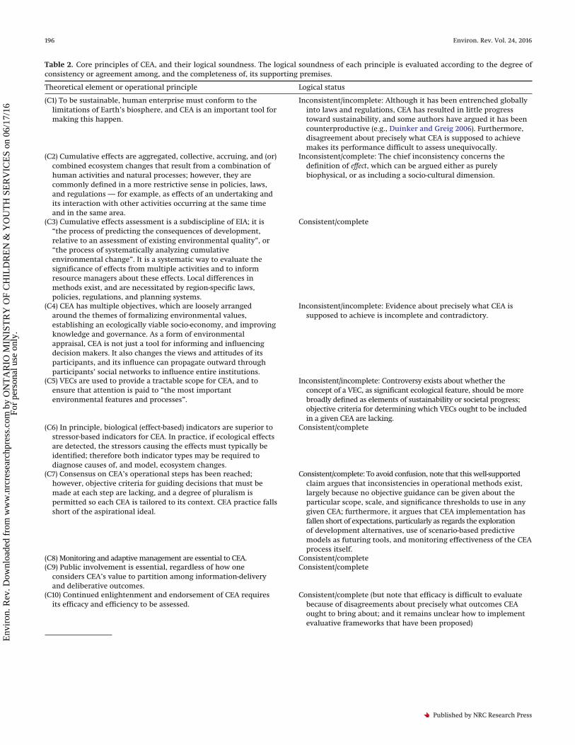
Table 2. Core principles of CEA, and their logical soundness. The logical soundness of each principle is evaluated according to the degree ofconsistency or agreement among, and the completeness of, its supporting premises.

Theoretical element or operational principle Logical status

(C1) To be sustainable, human enterprise must conform to thelimitations of Earth’s biosphere, and CEA is an important tool formaking this happen.

Inconsistent/incomplete: Although it has been entrenched globallyinto laws and regulations, CEA has resulted in little progresstoward sustainability, and some authors have argued it has beencounterproductive (e.g., Duinker and Greig 2006). Furthermore,disagreement about precisely what CEA is supposed to achievemakes its performance difficult to assess unequivocally.

(C2) Cumulative effects are aggregated, collective, accruing, and (or)combined ecosystem changes that result from a combination ofhuman activities and natural processes; however, they arecommonly defined in a more restrictive sense in policies, laws,and regulations — for example, as effects of an undertaking andits interaction with other activities occurring at the same timeand in the same area.

Inconsistent/complete: The chief inconsistency concerns thedefinition of effect, which can be argued either as purelybiophysical, or as including a socio-cultural dimension.

(C3) Cumulative effects assessment is a subdiscipline of EIA; it is“the process of predicting the consequences of development,relative to an assessment of existing environmental quality”, or“the process of systematically analyzing cumulativeenvironmental change”. It is a systematic way to evaluate thesignificance of effects from multiple activities and to informresource managers about these effects. Local differences inmethods exist, and are necessitated by region-specific laws,policies, regulations, and planning systems.

Consistent/complete

(C4) CEA has multiple objectives, which are loosely arrangedaround the themes of formalizing environmental values,establishing an ecologically viable socio-economy, and improvingknowledge and governance. As a form of environmentalappraisal, CEA is not just a tool for informing and influencingdecision makers. It also changes the views and attitudes of itsparticipants, and its influence can propagate outward throughparticipants’ social networks to influence entire institutions.

Inconsistent/incomplete: Evidence about precisely what CEA issupposed to achieve is incomplete and contradictory.

(C5) VECs are used to provide a tractable scope for CEA, and toensure that attention is paid to “the most importantenvironmental features and processes”.

Inconsistent/incomplete: Controversy exists about whether theconcept of a VEC, as significant ecological feature, should be morebroadly defined as elements of sustainability or societal progress;objective criteria for determining which VECs ought to be includedin a given CEA are lacking.

(C6) In principle, biological (effect-based) indicators are superior tostressor-based indicators for CEA. In practice, if ecological effectsare detected, the stressors causing the effects must typically beidentified; therefore both indicator types may be required todiagnose causes of, and model, ecosystem changes.

Consistent/complete

(C7) Consensus on CEA’s operational steps has been reached;however, objective criteria for guiding decisions that must bemade at each step are lacking, and a degree of pluralism ispermitted so each CEA is tailored to its context. CEA practice fallsshort of the aspirational ideal.

Consistent/complete: To avoid confusion, note that this well-supportedclaim argues that inconsistencies in operational methods exist,largely because no objective guidance can be given about theparticular scope, scale, and significance thresholds to use in anygiven CEA; furthermore, it argues that CEA implementation hasfallen short of expectations, particularly as regards the explorationof development alternatives, use of scenario-based predictivemodels as futuring tools, and monitoring effectiveness of the CEAprocess itself.

(C8) Monitoring and adaptive management are essential to CEA. Consistent/complete(C9) Public involvement is essential, regardless of how one

considers CEA’s value to partition among information-deliveryand deliberative outcomes.

Consistent/complete

(C10) Continued enlightenment and endorsement of CEA requiresits efficacy and efficiency to be assessed.

Consistent/complete (but note that efficacy is difficult to evaluatebecause of disagreements about precisely what outcomes CEAought to bring about; and it remains unclear how to implementevaluative frameworks that have been proposed)

196 Environ. Rev. Vol. 24, 2016

Published by NRC Research Press

Env

iron

. Rev

. Dow

nloa

ded

from

ww

w.n

rcre

sear

chpr

ess.

com

by

ON

TA

RIO

MIN

IST

RY

OF

CH

ILD

RE

N &

YO

UT

H S

ER

VIC

ES

on 0

6/17

/16

For

pers

onal

use

onl

y.

and decision makers (Harriman and Noble 2008; Gunn and Noble2009).

P90: Reciprocal learning can occur between project-based andmore strategic and regional forms of CEA (Connelly 2011; Seitzet al. 2011). “A regional approach can set the context needed forscoping, assessing and managing cumulative effects attributableto individual projects, whereas project-specific CEAs should buildon the regional understanding and suggest in some detail how tomanage the cumulative effects…(of a)…specific project” (Baxteret al. 2001).

C12: CEA is best undertaken in a strategic and regional context(Baxter et al. 2001); however, the current practice falls short ofideology (Gunn and Noble 2011).

P91: Planning is concerned with articulating societal prioritiesand managing change via the allocation of resources (Hegmannand Yarranton 2011); it establishes the context within with sus-tainability is to be implemented” (Gunn and Noble 2011).

P92: Responsibilities for EIA and CEA are more commonly thejurisdiction of “agencies having a development mandate, ratherthan an environmental mandate” (Pope et al. 2013). Regional plan-ning authorities are the “logical CEA proponents” (Gunn and Noble2009) because of the “unprecedented need for the integration ofsustainability principles in the development of regional policies,plans, and programs” (Gunn and Noble 2009).

P93: Instructive feedback loops exist between CEA and plan-ning. Sustainability goals provide a benchmark against which thesignificance of cumulative effects may be judged (Hegmann andYarranton 2011); whereas, CEA organizes, analyzes, and presentsinformation in a way that allows the sustainability of variousalternatives to be assessed (Hegmann and Yarranton 2011). Indeed,reciprocal feedback loops extend even more broadly across soci-etal domains and academic disciplines, because more, and better,CEA means that the outcomes of human activities can be betterpredicted. The more formal, quantitative, and strategic the plan-ning and regulatory process, the better CEA can be tuned, and themore meaningfully its performance can be evaluated (Duinkerand Greig 2007; Chapman and Maher 2014).

P94: Interdisciplinary communication and reciprocal learningpermit efficiency gains to accrue as CEA is iterated. For example,scenario development becomes more efficient and cost effectiveif premises, assumptions, and scenario types (e.g., “businessas usual”, “pessimistic”, “disastrous”, “optimistic”, or “mira-cle”; Cornish 2004; Duinker and Greig 2007) are shared.

C13: CEA and planning are inseparably linked, and communi-cation between these disciplines allows for reciprocal learning.

P95: The 96 premises and 13 conclusions listed here character-ize what CEA is, how and why it is done, and how and why it oughtto be done; however, these statements are incomplete and occa-sionally contradictory.

C14: As is true of EIA (Cashmore 2004), CEA’s theoretical basisis inadequately unified and detailed as “… a series of somewhatnebulous models operating along a broad spectrum of philosoph-ical beliefs and values”; Table 2).

CEA’s big problemsCEA should be innate. Our lives proceed via a great number of

decisions, the consequences of which are — or, at our own peril,are not — considered proactively. When the oven timer rings,signaling that the casserole is cooked, a plausible future scenarioincludes burnt hands and a trip to the emergency room. Burningthe hands leads to pain and misery, infection, loss of function, andultimately threatens survival (especially if done more than once).Prudent mitigation by the cook is achieved by donning oven mittsbefore dinner is removed from the oven. Difficulty with CEAarises when we scale up from the individual level to the collective,societal, and institutional levels. This scaling-up is most easilydone given an ethos of ethical objectivism, in which the collectivegood is paramount, principles of conservation or preservation arehighly valued, and individuals are held accountable to these mor-als. By contrast, many authors have argued that we are in an age ofindividualism, consumerism, cultural, and ethical relativism, andpersonal non-accountability (e.g., Rubin and Kaivo-Oja 1999; Truss2005; Hamilton 2010). These social viewpoints ultimately influ-ence CEA decisions because they influence how development-related trade-offs37 are perceived (Coates and Leahy 2006; Nunneriet al. 2008). Fully harnessing the potential of EIA and CEA assustainability instruments requires innovations that overcome,redirect, or reprogram these social norms.

Cumulative effects laws, regulations, and policies on their ownare universally incomplete and underachieve (Duinker and Greig2006). Furthermore, it is important to appreciate that in mostdemocracies the supreme constitutional principle is individualliberty. When implementing a regulation or law, the onus is onensuring protection of individual rights and freedoms (not theenvironment). For this reason, legislators often take an indirectapproach to environmental issues by prohibiting certain impacts,

37Trade-offs arise commonly in CEA where a favourable response in one indicator can only be achieved via the adverse response of another.

Table 2 (concluded).

Theoretical element or operational principle Logical status

(C11) Basic knowledge about ecological stressors and effects isrudimentary. Nonetheless, numerical methods for quantifying,assessing, modeling, and predicting cumulative effects are welldescribed. On one hand, our capacity for prediction is oftensmall, and there are practical limits to the number of factors thatcan be tested experimentally or modelled; on the other hand,crude approximation of cumulative effects is sufficient in mostCEA contexts.

Consistent/complete: The most significant problems with CEA arenot scientific.

(C12) CEA is best undertaken in a strategic and regional context, butthere are few examples of this in current practice.

Consistent/complete

(C13) CEA and planning are inseparably linked, and communicationbetween these disciplines allows for reciprocal learning.

Consistent/incomplete: The full case for integrating CEA andplanning has not yet been compiled. To avoid confusion, notethat the logical case for merging CEA and planning is consistent;however, examples of this marriage from current practice arerudimentary, in part because of institutional and jurisdictionalmismatches and inertia.

Jones 197

Published by NRC Research Press

Env

iron

. Rev

. Dow

nloa

ded

from

ww

w.n

rcre

sear

chpr

ess.

com

by

ON

TA

RIO

MIN

IST

RY

OF

CH

ILD

RE

N &

YO

UT

H S

ER

VIC

ES

on 0

6/17

/16

For

pers

onal

use

onl

y.

rather than limiting human activities (R. Cormier. pers. comm.2015). All the while, the blame-game circumvents meaningful con-frontation of cumulative effects: plan-makers argue that effectsare caused by individual actions, and individuals argue that theiractions are constrained by government policies (Therivel and Ross2007).

In addition, legal, regulatory, and institutional frameworks arelargely insufficient to enable CEA’s diverse outcomes to be real-ized (Ball et al. 2013), uncertainties about jurisdictional roles andresponsibilities are pervasive (especially when CEA is undertakenat a regional cross-jurisdictional scale; Damman et al. 1995), andconnections to science and planning are rudimentary. For exam-ple, the Chinese case study written by Wang et al. (2003) describeda series of systemic institutional problems, including project-based institutional attention being focused on air, water, and soilpollution, with social and ecological cumulative effects beinglargely ignored; complex and confusing lines of responsibility andaccountability that vary by jurisdiction, resulting in regional vari-ation in the quality of appraisals; waning institutional capacity,caused by insufficient funding as departmental responsibilitiesand workloads have expanded; perverse inter-agency incentivesthat arose from environmental regulators being funded by pollu-tion levies; and weak enforcement.

CEA does cultivate some obviously good practices. For example,it upholds informed, transparent, and accountable decision mak-ing, and it results in irreconcilable disputes being referred to thejudicial system (Hegmann and Yarranton 2011); however, appraisal,and its role in the decision-making process, is inadequately con-ceptualized (Owens et al. 2004), and its ostensive purposes aredifficult to translate into definable outcomes, so it is not clear howto use CEA to make demonstrably better decisions (Cashmore2004). CEA’s integration with the decision-making process stressesinformation delivery to decision makers, as a way of promotingrationality. But this is an unstable philosophical basis for CEA becauseit neither accounts accurately for the scientific assessment – decisionnexus (i.e., CEA rarely informs decisions in a straightforward lin-ear fashion, and decision makers fail to use vast quantities ofinformation produced for their use; Russell-Smith et al. 2015), norfor the decision-making systems that exist in modern democra-cies (in which there is no singular societal vision; Owens et al.2004). As a result, CEA is both naive and potentially dangerous —it allows “ethical and political choices (to) masquerade as techni-cal judgments” (Owens et al. 2004), and the resulting tokenismtends to reinforce a society’s norms and distribution of power(which are often at odds with CEA’s promise of sustainability).

In recent years, CEA has been seen in a new light, its focus “lesson an individual decision and more on long-term outcomesthrough processes of transformation” (Pope et al. 2013); thenagain, CEA (and EIA) have failed to realize their pledged delibera-tive outcomes. One of the main reasons for this deficiency is su-perficial public engagement, whereby members of the public areinvited only to review materials and provide comment (usuallytoo late in the CEA process to have much impact). For example,Sinclair et al. (2012) published (in the EIA literature) a particularlyscathing account of citizens’ experience in the Emera Brunswicknatural gas pipeline hearings in New Brunswick, Canada, whichshowed that “most elements of meaningful participation werenot satisfied”: information sessions intended to brief public par-ticipants were overly complicated, confusing, and formal, andfailed to prepare participants for the intimidating adversarial andquasi-judicial review process; funds provided to public partici-pants were meager, arrived too late in the process, and carried toomany conditions to level the playing field among parties to theappraisal; the review panel failed to adjust the scope of the assess-ment, despite repeated appeals from the public; time horizons for

phases of the appraisal, and hearing schedules, did not accommo-date the schedules of public participants (most of whom had full-time jobs and no staff to assist with preparation for hearings);open discussion about how issues raised during the process couldbe solved was discouraged by a review process that was based oncross-examination; and professionals in the process undervaluedlocal public knowledge (all of which left participants feeling “bit-ter, disrespected, marginalized, and wasted”. As several authorshave reported (Adelle and Weiland 2012; Pope et al. 2013) moreempowering and transformative models of engagement havebeen slow to catch on.

Aside from CEA’s theoretical basis, “resource-based targets orlimits are keys to stimulating careful thought about, and robustmanagement of, cumulative effects” (Therivel and Ross 2007)because they allow significance and acceptability to be specifiedquantitatively. Yet societies pay only lip service to the goal ofsustainability, and sustainability is not defined in a suitably opera-tional sense to provide a sound basis for CEA (Spaling et al. 2000;Connelly 2011; Hegmann and Yarranton 2011; Dubé et al 2013). Asa result, solutions to cumulative problems are often deemed un-palatable, their ownership is dismissed as someone else’s remit(Therivel and Ross 2007), and economic interests easily outweighenvironmental interests (e.g., Adelle and Weiland 2012). A varietyof methods exist for setting indicator targets relative to referencelevels or other baselines, nonlinear stressor–response relation-ships, and social norms38 (e.g., Samhouri et al. 2011); but there arealso a variety of challenges, as Samhouri et al. (2011) describedwith reference to marine-ecosystem targets for Puget Sound. Forexample, it is difficult to calibrate present ecosystem form orfunction to a historic or spatial reference condition in which hu-man impacts were absent. Furthermore ecosystems vary dynami-cally over time and space, meaning that historical and spatialbaselines are arbitrary.

Barriers to interdisciplinary research are another problem. AsRubin and Kaivo-Oja (1999) wrote, “the boundaries between natu-ral sciences, social sciences, and the humanities…have blurred”,and this blurring needs to take place given that complex sustain-ability problems have to be solved by changing the interactionsbetween social and ecological systems (Klein 2004; Binder et al.2013); however, methods of interdisciplinary research and collab-oration are rudimentary (e.g., Sheate 2010; Morrison-Saunderset al. 2014), and disincentives abound — for example, obstructiveprejudgments that social and natural scientists make about oneanother, the lack of opportunities for financing interdisciplinarywork, differing discipline-specific publishing expectations, powerdifferentials that exist in diverse research collaborations, and theneed for time-consuming procedures to manage team dynamicsand clearly articulate research goals and methods (Campbell 2005;Morse et al. 2007).

Many how-to documents have been written for CEA practitio-ners (e.g., Hegmann et al. 1999; Cooper 2004; Munier 2004;Glasson et al. 2013), but guidance on how to operationalize CEAremains incomplete and difficult to generalize, and a variety ofmethodological challenges remain. This is true because decisionshave to be made at each step of the CEA process, but objective anduniversal criteria for guiding those decisions do not exist. Societalvalues and sustainability goals vary from place to place, whichmeans that the scope of issues to include in CEA assessments isimpossible to standardize, as are decisions about which VECs andindicators to use (e.g., Baxter et al. 2001; Therivel and Ross 2007,Ball et al. 2013). The outcome of this subjectivity is that VECs areoften included only if significantly impacted by the undertak-ing(s) being appraised, so environmental components that areincrementally affected in a minor way are excluded, and deaths bya thousand cuts can continue unabated (Bérubé 2007). Further-

38Social norms define what is generally excepted within a given cultural setting, and can be quantified statistically from survey data (Samhouri et al. 2011).

198 Environ. Rev. Vol. 24, 2016

Published by NRC Research Press

Env

iron

. Rev

. Dow

nloa

ded

from

ww

w.n

rcre

sear

chpr

ess.

com

by

ON

TA

RIO

MIN

IST

RY

OF

CH

ILD

RE

N &

YO

UT

H S

ER

VIC

ES

on 0

6/17

/16

For

pers

onal

use

onl

y.

more, the appropriate spatial and temporal scale for a given CEAdepends on the subject of the CEA appraisal, and on selected VECsand indicators, among other factors; however, chosen surrogateindicators may not be predictable enough to be used in CEA sce-nario models, and ecological indicators that can be modeled withsuitable precision may not be relevant to local VECs. Objectivethresholds for the significance of effects are elusive given ambi-guity of the term threshold, and the fuzziness of sustainabilitygoals (McCold and Saulsbury 1996; Bérubé 2007; Ball et al. 2013).Methods of evaluating performance are difficult to standardizebecause CEA’s pluralistic information-delivery and social out-comes are treated as more or less legitimate by different authors.

According to Schultz (2012), “determining the appropriate geo-graphic and temporal scales of analysis is one of the most perplex-ing aspects of CEA”. This is partially because stressors and effectscommonly occur at different spatial and temporal scales (Seitzet al. 2011), but also because the larger the area covered by a CEA,the less important local issues (e.g., a new factory or shoppingmall) will be, the more important landscape-scale phenomena(e.g., pervasive impacts associated with the manufacturing orcommercial sector) will be, the less likely it will be that a partic-ular effect will be singled out as significant, the less likely it will bethat CEA boundaries will align with administrative ones, and theless clear it will be where the responsibility for follow-up actionlies. Similarly, the longer the timeframe considered, the less cer-tain CEA analyses will be (Therivel and Ross 2007; Seitz et al. 2011).

Mathematical procedures for associating stressors and effectsare relatively well described, but the required monitoring data aregenerally lacking (Damman et al. 1995; Scherer 2011; Schultz 2012;Ball et al. 2013; Venier et al. 2014), and are “expensive and timeconsuming to gather” (Connelly 2011). Obviously, more complexmodels call for more complex input datasets and underlying mon-itoring programs, so a vicious cycle is apparent (Gallagher et al.2015). The information that is available is “highly uncertain andvariable in quality” (Karkkainen 2002), and is, for the most part,not efficiently shared among CEA participants (Damman et al.1995).

Hutchinson’s (1959) concept of the niche provides a strong the-oretical basis for thresholds, because it posits that organisms cantolerate only a finite range of conditions relative to any environ-mental dimension; however, in practice, multiple definitions ofthe term threshold exist. For example, the term can be used todescribe a fundamental shift in community structure or dynamics,or a nonlinear response of a population to one or more distur-bances. Furthermore, there are many levels of biological organi-zation at which thresholds may be evident; there are a limitlessnumber of potential response variables for which thresholdscould be derived; and different statistical approaches will result indifferent thresholds. Exploring only a small number of these iscostly and requires an immense amount of data, but only a smallsubset of identified thresholds will be relevant to VEC conserva-tion (Johnson 2013). Statistical significance may be easy to demon-strate, for example, as the value of a given indicator being outsideof a statistically defined “normal” (e.g., Kilgour et al. 1998), butecological significance is another matter. Furthermore, the soci-etal significance and relevance of a cumulative effect is open todebate, given how vague the concept of sustainability is (Scherer2011; Moldan et al. 2012).

In addition to the subjectivity of decisions made in the CEAprocess, complexity and uncertainty are fundamental difficulties,commonly invoked to describe, for example, the diversity of bio-logical and physical land-use effects, stressor interactions, spatialand temporal lags between stressors and effects, nonlinear rela-

tionships, and positive and negative feedback loops (Spaling andSmit 1993; Therivel and Ross 2007; Seitz et al. 2011; Ball et al. 2013).In Hegmann and Yarranton’s (2011) pessimistic assessment, “evenif practitioners employ the most advanced and complex analysisand the best that analytical thought may offer (CEA) still deliversjust words and numbers buried within limitations, assumptionsand uncertainties” (Hegmann and Yarranton 2011).

It is clear that CEA’s big problems are not discrete. Rather, theyoverlap and feed off each other. They are also replicated through-out the other subdisciplines of EIA, where they have caused con-fusion and exaggerated methodological incompatibilities (Canteret al. 2010; Morrison-Saunders et al. 2014).

Recommendations

CEA should be considered one part of a precautionarysustainability strategy, not as a standalone solution fordealing with development-related environmental effects

Earth can neither support our current resource demands norassimilate the ecological stresses associated with further de-mands (Wackernagel and Rees 1998). Ecological trends suggestdeepening unsustainability (Vitousek et al. 1997; Foley et al. 2005;Steffen et al. 2007). We are caught in a vicious cycle of ecologicalexploitation that leads to ecosystem damage, the exhaustion ofresources, and a spiral of continuing degradation, as livelihoodsare undermined (Schnaiberg and Gould 2000; Gibson 2012). Envi-ronmental conservation and development may both be seen associetal imperatives, but ecological considerations ultimatelymust be the trump card. Proposed human endeavors should moveforward only if they are expected to pay long-term ecological div-idends. A mitigative approach, which slows down incrementallosses, is inadequate because it falls short of the principle of nonet loss (e.g., Benson 2003), and the needed reversals of presentecological trajectories (Bond et al. 2012). As a starting point, thesustainability goals of the United Nations General Assembly(UNGE 2015), which are largely directed at the world’s govern-ments, may help to change societal values so they become morealigned with CEA. Furthermore, the influence of the UN targetscould be maximized by also mobilizing extra-governmental advo-cates for change, which Hajer et al. (2015) suggested could be doneby invoking complementary notions, such as “planetary boundar-ies” (which stress the urgency of environmental concerns and theneed to take responsibility for ecosystem goods and services), “thesafe and just operating space” (which highlights interconnected-ness of social and environmental concerns), and “the energeticsociety” (which stimulates “green competition” and technologicalinnovation). All of these concepts should be operationalized withrelevant indicators and monitoring (e.g., Hák et al. 2016), some ofwhich will be of use in CEA.

Recognize that people and political systems are notprogrammed to think in terms of long-term strategy (e.g.,Diamond 2005), and do not allow CEA (or EIA) to usurpprecaution39

Considerable societal inertia exists that is counter to the prin-ciples of sustainability, and EIA’s forty-year track record is notstellar. There is, however, hope for CEA, which can be viewed as away to enforce strategic thinking.

As regards development, logically sound precaution should beoperationalized in the decision making process as: avoid, minimize,restore, offset. CEA traditionally encompasses the first two of thesestrategies. Compensatory restoration and offsets (e.g., Theriveland Ross 2007; Connelly 2011) are much-needed complements,which are consistent with the idea of no net loss, and can “make

39Precaution is used here in the legal sense, as a principle that “ensures that a substance or activity posing a threat to the environment is prevented fromadversely affecting the environment, even if there is no conclusive scientific proof linking that particular substance or activity to environmental damage”(Cameron and Abouchar 1991).

Jones 199

Published by NRC Research Press

Env

iron

. Rev

. Dow

nloa

ded

from

ww

w.n

rcre

sear

chpr

ess.

com

by

ON

TA

RIO

MIN

IST

RY

OF

CH

ILD

RE

N &

YO

UT

H S

ER

VIC

ES

on 0

6/17

/16

For

pers

onal

use

onl

y.

room” for future developments (Canter and Ross 2010) where fur-ther consumptive expansion is justifiable because of current de-ficiency. CEA should therefore be used to transition fromconsumptive to non- or less-consumptive means of enhancinghuman expression and wellbeing.

In general, any measures to protect more areas and concentratedevelopment in areas that are already disturbed warrant atten-tion (e.g., Venier et al. 2014). New roads and development in pre-viously remote areas should be avoided, because opening upaccess causes chain reactions of effects (Cochrane and Laurance2008; Fraser 2014). Similarly, Bond and co-authors’ (2012) rulesabout how to handle trade-offs warrant implementation: an ac-ceptable trade-off is defined as delivering net long-term sustain-ability gains; no trade-off involving significant adverse effects isacceptable, and no displacement of adverse impacts into the fu-ture is tolerable “unless all other alternatives are worse”; when atrade-off is proposed, its justification is the responsibility of theproponent, and this justification must be reviewed in an openparticipatory process, relative to established decision criteria. Ul-timately, planning and regulatory instruments should includelimits40 (e.g., Johnson 2013) on population and developed land(Hegmann and Yarranton 2011) as a way to stimulate innovationand prevent the death by a thousand cuts.

Societies should better integrate CEA and planning (i.e.,CEA should be viewed as both a tool for plan creation andevaluation), and should set clear targets for social–cultural,economic, and ecological indicators

Better consolidating CEA and planning would create a “verti-cally integrated framework” (Pope et al. 2013) in which environ-mental and sustainability issues could be considered withappropriate detail at appropriate levels of decision making. Itcould also benefit both processes by helping to clarify sustainabil-ity goals and uncovering (and putting to practical use) meaningfulthresholds for important indicators of ecological and social well-being (Hegmann and Yarranton 2011). Articulating sustainabilitygoals, and implementing them as regulatory limits (e.g., Johnson2013), would lend administrative efficiency to CEA. This wouldalleviate the tendency for organizations to demand onerous ap-praisals as a way to compensate for inadequate policies and con-flicting views of sustainability (Hegmann and Yarranton 2011). Itwould also greatly simplify evaluations of CEA performance. Fur-thermore, beneficial spin-offs outside of CEA would accrue, be-cause targets remove ambiguity from well-intended but vaguepolicy statements, which facilitates strategic planning and providesantecedents for complementary laws and regulations (Samhouriet al. 2011).

Consider environmental appraisal and planning to be toolsfor managing change, not development

Encouraging development where it makes sense to do so, andconstraining it where unacceptable trade-offs are likely to resultshould be pursued to the extent possible (Hegmann and Yarranton2011). The goal should be “qualitative rather than quantitativegrowth”41 (Häyhä and Franzese 2014).

If the chief purpose of CEA is to enforce evidence-basedrationality, then formalize quantitative rules in thedecision-making process

Evidence-based decision making demands trade-offs to be de-fined and revealed through a structured process (Johnson 2013),and targets are a critical part of this process. Even a vague, quali-tative target can stimulate policy debate and research concerningdesirable and undesirable end-points. Beyond this, evidence-based decision making can be formalized and quantified by mea-suring indicator distances to the target (Moldan et al. 2012).Control charts (i.e., time-series plots showing trends in VEC con-dition, relative to acceptable limits) should be hanging on board-room walls. Referring to such charts would help to enforcerationality by drawing decision makers’ attention to their ownbiases (e.g., Rubin and Kaivo-Oja 1999), while promoting “futures-oriented thinking” (Masini 1993), and focussing debate on trade-offs. By this method, human activities would be assessed on adistance-to-target basis (e.g., Moldan et al. 2012) and approved iftheir predicted effects did not exceed a pre-defined regulatorylimit, which Johnson (2013) suggested could be set relative tomodels of ecological response, socioeconomic trade-offs, andtechnological best practices. Johnson’s (2013) uncertainty-basedguidance illustrated how such control charts could be interpretedin relation to “critical limits” (a point at which a VEC is nearingunacceptable change), “target limits” (which operationalize anacceptable amount of VEC change, relative to ecological and so-cioeconomic realities), and “cautionary limits” (which identifyecological or socioeconomic changes that require adaptive moni-toring).

Maximize opportunities for deliberation in CEA, because itsdeliberative outcomes — which include and require debate,collaboration, creativity, learning, exposure to differentworld views, and consideration of the distribution of poweramong decision makers — have the greatest potential torevolutionize our approach to sustainability

Given damning critiques of the concept of rational information-based decision making, various authors have emphasized theneed for “new thinking about planning and decision making pro-cesses in their wider social, cultural, political and economic con-texts” (Morgan 2012). One of the major problems with the modelof information-based decision making in CEA is that it subvertsmeaningful civic debate by disguising development options asbeing merely technical, rather than political. Unfortunately, nobetter model has come to light (Owens et al. 2004; Bond and Pope2012): more political views of the decision-making process, forexample, are called out as being naive because their proponentsexpect a difficult, time-consuming, expensive, and potentiallyinconclusive process of deliberation to result in clear recommen-dations and actions (Owens et al. 2004). Regardless, information-based appraisals, and appraisals that stress the deliberativeprocess, are not mutually exclusive, and providence calls for CEAto derive its knowledge-based products from a process that is asinclusive as possible, and seeks to maximize creativity and oppor-tunities for collaboration and open dialogue among its partici-pants (e.g., Bartlett and Kurian 1999; Adelle and Weiland 2012;Folkeson et al. 2013; Ball et al. 2013). Novel forms of “ad hoc delib-

40Johnson (2013) defined regulatory limit as “the magnitude or extent of human disturbance that is permitted, after which unacceptable ecological changeor …. risk is expected”.41This turn of phrase from Häyhä and Franzese (2014) was made while contrasting flows of different types of capital in what they referred to as “strong” and“weak” systems of sustainability. Re-stating their comment, strong sustainability considers natural capital (local ecosystems, biomes, sub-soil resources) tobe irreplaceable, whereas weak sustainability assumes that technological substitutes can be found for lost natural capital. Strongly sustainable (“qualita-tive”) development, then converts natural capital to manufactured capital (e.g., roads, buildings) so as to maximize positive spin-offs to human capital (e.g.,knowledge), and social capital (institutional capacity); and this conversion of natural capital is constrained by its natural rate of regeneration. TheEcological Footprint concept of sustainability (i.e., Wackernagel and Rees 1998) takes a similar view, thus a city is sustainably developed so long as itsfootprint does not exceed the area of biosphere required to produce its raw materials.

200 Environ. Rev. Vol. 24, 2016

Published by NRC Research Press

Env

iron

. Rev

. Dow

nloa

ded

from

ww

w.n

rcre

sear

chpr

ess.

com

by

ON

TA

RIO

MIN

IST

RY

OF

CH

ILD

RE

N &

YO

UT

H S

ER

VIC

ES

on 0

6/17

/16

For

pers

onal

use

onl

y.

eration” have been advocated as one promising approach to com-plement regulated consultation and boost deliberative outcomes(i.e., Folkeson et al. 2013).

Continue to reason through CEA’s operational challenges,and update guidance documents where possible (Connelly2011), as a way of ushering in a more enlightened CEA

Many operational challenges and shortcomings of CEA guid-ance documents arise because objective decision criteria (e.g., inrelation to scope, scale, and thresholds) are nonexistent. The re-gional variability of CEA requirements is a further complication,because it precludes generalization. Regardless, there are stillplenty of opportunities for innovation. Researching methods bywhich trade-offs can be optimized quantitatively may be a prom-ising approach. For example, ways of optimizing spatial and tem-poral scale relative to the uncertainty and significance of effectswould be helpful, as would procedures that align CEA’s spatialboundaries with VECs (Baxter et al. 2001), and with the presum-able geographic extent of stressors and effects (Seitz et al. 2011;Ball et al. 2013).

Improve monitoring systemsLack of data is a universal complaint among CEA practitioners.

Regional monitoring programs that are interwoven with researchagendas, planning and regulatory processes, and are supportedwith long-term funding, robust data-management, and data-sharing systems should be implemented widely (Ball et al. 2013;Dubé et al. 2013). Such programs stand to benefit many elementsof CEA, by characterizing baseline conditions, detecting and de-scribing trends, permitting stressors and effects to be associated(Seitz et al. 2013), and enabling adaptive management (Karkkainen2002).

Consolidate good practices among EIA disciplinesReturning to the basics with a refocusing on better scoping and

the sustainability ideal would inspire practitioners intellectually,and would uncover different ways of looking at the same prob-lem, which would benefit EIA and all of its subdisciplines (Canteret al. 2010; Sheate 2010; Morrison-Saunders et al. 2014).

Continue to work on critical science questionsIn particular, continue to investigate and theorize how environ-

mental appraisal and decision-making interrelate (Cashmore2004; Bond and Pope 2012), and continue to elucidate links be-tween stressors and effects, which will enhance our capacity forprediction.

Foster interdisciplinarity among CEA researchers and theirinstitutions

Interdisciplinary study of CEA’s role in socio-ecological systemsis equally important as discipline-specific research (Leknes 2001;Cashmore 2004). EIA researchers should establish interdisciplin-ary teams, governed by accountability and communication strat-egies that maximize reciprocal learning and define expectedoutcomes and timelines. Academic institutions should providetraining and mentorship opportunities in interdisciplinary re-search (Morse et al. 2007).

AcknowledgementsThe logical argument (conceptual model) presented in this pa-

per was refined via discussions among members of the MuskokaRiver Watershed CEA Research Consortium, and by feedback re-ceived from audience members at several conferences and meet-ings where earlier versions were presented. I thank the followingcolleagues for sharing their perspectives: Judi Brouse, RolandCormier, Simon Courtenay, Christy Doyle, Cathy Eimers, LorneGreig, Gary Lovett, Scott MacRitchie, Andrew Paterson, Jim Rusak,Peter Sale, Keith Somers, Lisa Trevisan, and Norman Yan. I amgrateful to Robert Gibson and two anonymous reviewers for their

constructive suggestions, which greatly enhanced the manu-script. This work was funded, in part, by a grant from the Cana-dian Water Network.

ReferencesAdelle, C., and Weiland, S. 2012. Policy assessment: the state of the art. Impact

Assess. Project Appraisal. 30(1): 25–33. doi:10.1080/14615517.2012.663256.Atkinson, S.F., and Canter, L.W. 2011. Assessing the cumulative effects of proj-

ects using geographic information systems. Environ. Impact Assess. Rev.31(5): 457–464. doi:10.1016/j.eiar.2011.01.008.

Ball, M., Somers, G., Wilson, J.E., Tanna, R., Chung, C., Duro, D.C., and Seitz, N.2013. Scale, assessment components, and reference conditions: issues forcumulative effects assessment in Canadian watersheds. Integr. Environ. As-sess. Manage. 9(3): 370–379. doi:10.1002/ieam.1332.

Bartlett, R.V., and Kurian, P.A. 1999. The theory of environmental impact assess-ment: implicit models of policy making. Policy Politics, 27(4): 415–433. doi:10.1332/030557399782218371.

Baxter, W., Ross, W.A., and Spaling, H. 2001. Improving the practice of cumula-tive effects assessment in Canada. Impact Assess. Project Appraisal, 19(4):253–262. doi:10.3152/147154601781766916.

Beanlands, G.E., and Duinker, P.N. 1983. An ecological framework for environ-mental impact assessment in Canada. Federal Environmental AssessmentReview Office, Hull, Quebec.

Benson, J.F. 2003. What is the alternative? Impact assessment tools and sustain-able planning. Impact Assess. Project Appraisal, 21(4): 261–280. doi:10.3152/147154603781766185.

Bérubé, M. 2007. Cumulative effects assessments at Hydro-Québec: what havewe learned? Impact Assess. Project Appraisal, 25(2): 101–109. doi:10.3152/146155107X197913.

Binder, C.R., Hinkel, J., Bots, P.W., and Pahl-Wostl, C. 2013. Comparison of frame-works for analyzing social-ecological systems. Ecol. Soc. 18(4): 26. doi:10.5751/ES-05551-180426.

Birkeland, J. 1999. Community participation in urban project assessment(an ecofeminist analysis). In Technology and Public Participation. Edited byB. Martin. University of Wollongong. pp. 113–142.

Bonada, N., Prat, N., Resh, V.H., and Statzner, B. 2006. Developments in aquaticinsect biomonitoring: a comparative analysis of recent approaches. Annu.Rev. Entomol. 51: 495–523. doi:10.1146/annurev.ento.51.110104.151124. PMID:16332221.

Bond, A.J. 2003. Let’s not be rational about this: response to Benson. ImpactAssess. Project Appraisal, 21(4): 266–268.

Bond, A., and Pope, J. 2012. The state of the art of impact assessment in 2012.Impact Assess. Project Appraisal, 30(1): 1–4. doi:10.1080/14615517.2012.669140.

Bond, A., Morrison-Saunders, A., and Pope, J. 2012. Sustainability assessment:the state of the art. Impact Assess. Project Appraisal, 30(1): 53–62. doi:10.1080/14615517.2012.661974.

Borja, A., Barbone, E., Basset, A., Borgersen, G., Brkljacic, M., Elliott, M.,Garmendia, J.M., Marques, J.C., Mazik, K., Muxika, I., et al. 2011. Response ofsingle benthic metrics and multi-metric methods to anthropogenic pressuregradients, in five distinct European coastal and transitional ecosystems.Mar. Pollut. Bull. 62(3): 499–513. doi:10.1016/j.marpolbul.2010.12.009. PMID:21215975.

Boulding, K.E. 1966. The economics of the coming spaceship earth. In Environ-mental Quality in a Growing Economy. Edited by H. Jarret. John HopkinsUniversity Press, Baltimore. pp. 3–14.

Brundtland, G.H. 1987. Our common future. World Commission on Environ-ment and Development: Brussels. Available from http://www.bne-portal.de/fileadmin/unesco/de/Downloads/Hintergrundmaterial_international/Brundtlandbericht.File.pdf?linklisted=2812 [accessed 17 October 2015].

Burton, G.A., Jr., Chapman, P.M., and Smith, E.P. 2002. Weight-of-evidence ap-proaches for assessing ecosystem impairment. Hum. Ecol. Risk Assess.: Int. J.8: 1657–1673. doi:10.1080/20028091057547.

Cairns, J., Jr., McCormick, P.V., and Niederlehner, B.R. 1993. A proposed frame-work for developing indicators of ecosystem health. Hydrobiologia, 263(1):1–44. doi:10.1007/BF00006084.

Cameron, J., and Abouchar, J. 1991. Precautionary principle: a fundamental prin-ciple of law and policy for the protection of the global environment. BostonColl. Int. Comp. Law Rev. 14(1): 1–27.

Campbell, L.M. 2005. Overcoming obstacles to interdisciplinary research. Con-serv. Biol. 19(2): 574–577. doi:10.1111/j.1523-1739.2005.00058.x.

Canter, L.W., and Atkinson, S.F. 2011. Multiple uses of indicators and indices incumulative effects assessment and management. Environ. Impact Assess.Rev.31(5): 491–501. doi:10.1016/j.eiar.2011.01.012.

Canter, L., and Ross, B. 2010. State of practice of cumulative effects assessmentand management: the good, the bad and the ugly. Impact Assess. ProjectAppraisal, 28(4): 261–268. doi:10.3152/146155110X12838715793200.

Canter, L., Atkinson, S.F., and Sadler, B. 2010. Introduction to a special issue oncumulative effects assessment and management. Impact Assess. Project Ap-praisal, 28(4): 259–260. doi:10.3152/146155110X12881021614499.

Cashmore, M. 2004. The role of science in environmental impact assessment:process and procedure versus purpose in the development of theory. Envi-ron. Impact Assess. Rev. 24(4): 403–426. doi:10.1016/j.eiar.2003.12.002.

Jones 201

Published by NRC Research Press

Env

iron

. Rev

. Dow

nloa

ded

from

ww

w.n

rcre

sear

chpr

ess.

com

by

ON

TA

RIO

MIN

IST

RY

OF

CH

ILD

RE

N &

YO

UT

H S

ER

VIC

ES

on 0

6/17

/16

For

pers

onal

use

onl

y.

CEARC (Canadian Environmental Assessment Research Council). 1988. The as-sessment of cumulative effects: a research prospectus. Canadian Environ-mental Assessment Research Council, Hull, Quebec.

Chapman, P.M., and Maher, B. 2014. The need for truly integrated environmen-tal assessments. Integr. Environ. Assess. Manage. 10(2): 151. doi:10.1002/ieam.1532.

Coates, J., and Leahy, T. 2006. Ideology and politics: Essential factors in the pathtoward sustainability. Electron. Green J. 1(23).

Cochrane, M.A., and Laurance, W.F. 2008. Synergisms among fire, land use, andclimate change in the Amazon. AMBIO: J. Hum. Environ. 37(7): 522–527.doi:10.1579/0044-7447-37.7.522. PMID:19205173.

Cocklin, C., Parker, S., and Hay, J. 1992. Notes on cumulative environmentalchange I: concepts and issues. J. Environ. Manage. 35(1): 31–49. doi:10.1016/S0301-4797(05)80126-4.

Connelly, R.B. 2011. Canadian and international EIA frameworks as they apply tocumulative effects. Environ. Impact Assess. Rev. 31(5): 453–456. doi:10.1016/j.eiar.2011.01.007.

Cooper, L.M. 2004. Guidelines for Cumulative Effects Assessment in SEA ofPlans. EPMG Occasional Paper 04/LMC/CEA, Imperial College London. Avail-able from http://www.imperial.ac.uk/pls/portallive/docs/1/21559696.PDF [ac-cessed 18 October 2015].

Cormier, S.M., and Suter, G.W., II. 2008. A framework for fully integrating envi-ronmental assessment. Environ. Manage. 42(4): 543–556. doi:10.1007/s00267-008-9138-y. PMID:18506517.

Cornish, E. 2004. Futuring: The exploration of the future. World Future Society,Bethesda, MarylandD.

Costanza, R. 1992. Ecological economics: the science and management of sus-tainability. Columbia University Press.

Culhane, P.J. 1990. NEPA’s impacts on federal agencies, anticipated and unan-ticipated. Environ. Law, 20(681): 690–93.

Daly, H. 1977. Steady-State Economics. W.H. Freeman and Co., San Francisco.Damman, D.C., Cressman, D.R., and Sadar, M.H. 1995. Cumulative effects assess-

ment: the development of practical frameworks. Impact Assess. 13(4): 433–454. doi:10.1080/07349165.1995.9726112.

Davenport, T.E., Meals, D.W., and Dressing, S.A. 2008. Monitoring, modeling anddecision making: making it work. NMQMC Sixth National Monitoring Con-ference. Available from http://acwi.gov/monitoring/conference/2008/papers/I2-D.pdf [accessed 16 October 2015].

Dawe, N.K., and Ryan, K.L. 2003. The faulty three-legged-stool model of sustain-able development. Conserv. Biol. 17(5): 1458–1460. doi:10.1046/j.1523-1739.2003.02471.x.

De Martino, B., Kumaran, D., Seymour, B., and Dolan, R.J. 2006. Frames, biases,and rational decision-making in the human brain. Science, 313(5787): 684–687. doi:10.1126/science.1128356. PMID:16888142.

Diamond, J.M. 2005. Collapse: How societies choose to fail or succeed. Viking,New York.

Dolédec, S., Phillips, N., Scarsbrook, M., Riley, R.H., and Townsend, C.R. 2006.Comparison of structural and functional approaches to determining landuseeffects on grassland stream invertebrate communities. J. N. Am. Benth. Soc.25(1): 44–60. doi:10.1899/0887-3593(2006)25[44:COSAFA]2.0.CO;2.

Doyle, J. 1999. Rational decision making. In MIT encyclopedia of the cognitivesciences. Edited by R.A. Wilson and F.C. Keil. MIT Press, Cambridge, Massachu-setts. pp. 701–703.

Dubé, M.G. 2003. Cumulative effect assessment in Canada: a regional frameworkfor aquatic ecosystems. Environ. Impact Assess. Rev. 23(6): 723–745. doi:10.1016/S0195-9255(03)00113-6.

Dubé, M., Johnson, B., Dunn, G., Culp, J., Cash, K., Munkittrick, K., Wong, I.,Hedley, K., Booty, W., Lam, D., et al. 2006. Development of a new approach tocumulative effects assessment: a northern river ecosystem example. Envi-ron. Monit. Assess. 113(1–3): 87–115. doi:10.1007/s10661-005-9098-0. PMID:16532283.

Dubé, M., Duinker, P., Grieg, L., Carver, M., Servos, M., McMaster, M., Noble, B.,Schreier, H., Jackson, L., and Munkittrick, K.R. 2013. A framework for assess-ing cumulative effects in watersheds: an introduction to Canadian case stud-ies. Integr. Environ. Assess. Manage. 9(3): 363–369. doi:10.1002/ieam.1418.

Duinker, P.N., and Greig, L.A. 2006. The impotence of cumulative effects assess-ment in Canada: ailments and ideas for redeployment. Environ. Manage.37(2): 153–161. doi:10.1007/s00267-004-0240-5. PMID:16362488.

Duinker, P.N., and Greig, L.A. 2007. Scenario analysis in environmental impactassessment: Improving explorations of the future. Environ. Impact Assess.Rev. 27(3): 206–219. doi:10.1016/j.eiar.2006.11.001.

Elkington, J. 1997. Cannibals with forks. The triple bottom line of 21st century.Capstone, Oxford, UK.

Ellis, E.C. 2011. Anthropogenic transformation of the terrestrial biosphere. Phi-los. Trans. R. Soc. A, 369(1938): 1010–1035. doi:10.1098/rsta.2010.0331.

Etzioni, A. 1988. Normative-affective factors: toward a new decision-makingmodel. J. Econ. Psy. 9: 125–150. doi:10.1016/0167-4870(88)90048-7.

EU (European Union). 1985. European Union Environmental Impact AssessmentDirective (85/337/EEC), Annex III, CELEX No. 31985L033727, June 1985. Avail-able from http://eur-lex.europa.eu/legal-content/EN/TXT/?uri=CELEX:31985L0337 [accessed 16 October 2015].

Fisher, S.R.A. 1960. The design of experiments (Vol. 12, No. 6). Oliver and Boyd,Edinburgh.

Fisheries and Oceans Canada. 2004. Identification of Ecologically and Biologi-cally Significant Areas. National Capital Region. Ecosystem Status Report2004/006. Available from http://www.dfo-mpo.gc.ca/csas/Csas/status/2004/ESR2004_006_E.pdf [accessed 16 October 2015].

Fisheries and Oceans Canada. 2011. Identification of Ecologically and Biologi-cally Significant Areas —Lessons Learned. Department of Fisheries andOceans Canada, Science Advisory Section, Scientific Advisory Report 2011/049. Available from http://www.dfo-mpo.gc.ca/csas-sccs/Publications/SAR-AS/2011/2011_049-eng.pdf [accessed 16 October 2015].

Fisheries and Oceans Canada. 2014. Assessment of Freshwater Ecologically andBiologically Significant Areas (EBSA) and Ecologically Significant Species(ESS) criteria. Department of Fisheries and Oceans Canada, Science AdvisorySection, Scientific Advisory Report 2014/025. Available from http://publications.gc.ca/collections/collection_2014/mpo-dfo/Fs70-6-2014-025-eng.pdf [accessed 16 October 2015].

Foley, J.A., DeFries, R., Asner, G.P., Barford, C., Bonan, G., Carpenter, S.R.,Chapin, S., Coe, M.T., Daily, G.C., Gibbs, H.K., et al. 2005. Global consequencesof land use. Science, 309(5734): 570–574. doi:10.1126/science.1111772. PMID:16040698.

Folkeson, L., Antonson, H., and Helldin, J.O. 2013. Planners’ views on cumulativeeffects. A focus-group study concerning transport infrastructure planning inSweden. Land Use Policy, 30(1): 243–253. doi:10.1016/j.landusepol.2012.03.025.

Fraser, B. 2014. Deforestation: Carving up the Amazon. Nature, 509(7501): 418–419. doi:10.1038/509418a. PMID:24848046.

Gallagher, S.S., Rice, G.E., Scarano, L.J., Teuschler, L.K., Bollweg, G., andMartin, L. 2015. Cumulative risk assessment lessons learned: A review ofcase studies and issue papers. Chemosphere, 120: 697–705. doi:10.1016/j.chemosphere.2014.10.030. PMID:25462315.

Gibson, R.B. 2012. In full retreat: the Canadian government’s new environmen-tal assessment law undoes decades of progress. Impact Assess. Project Ap-praisal, 30(3): 179–188. doi:10.1080/14615517.2012.720417.

Glasson, J., Therivel, R., and Chadwick, A. 2013. Introduction to environmentalimpact assessment, fourth edition. Routledge, London, UK.

Gunn, J.H., and Noble, B.F. 2009. A conceptual basis and methodological frame-work for regional strategic environmental assessment (R-SEA). Impact Assess.Project Appraisal. 27(4): 258–270. doi:10.3152/146155109X479440.

Gunn, J., and Noble, B.F. 2011. Conceptual and methodological challenges tointegrating SEA and cumulative effects assessment. Environ. Impact Assess.Rev. 31(2): 154–160. doi:10.1016/j.eiar.2009.12.003.

Hajer, M., Nilsson, M., Raworth, K., Bakker, P., Berkhout, F., de Boer, Y.,Rockström, J., Ludwig, K., and Kok, M. 2015. Beyond Cockpit-ism: Four In-sights to Enhance the Transformative Potential of the Sustainable Develop-ment Goals. Sustainability, 7(2): 1651–1660. doi:10.3390/su7021651.

Hák, T., Janoušková, S., and Moldan, B. 2016. Sustainable Development Goals: Aneed for relevant indicators. Ecol. Indic. 60: 565–573. doi:10.1016/j.ecolind.2015.08.003.

Hamilton, C. 2010. Consumerism, self-creation and prospects for a new ecolog-ical consciousness. J. Cleaner Prod. 18(6): 571–575. doi:10.1016/j.jclepro.2009.09.013.

Harriman, J.A., and Noble, B.F. 2008. Characterizing project and strategic ap-proaches to regional cumulative effects assessment in Canada. J. Environ.Assess. Policy Manage. 10(1): 25–50. doi:10.1142/S1464333208002944.

Häyhä, T., and Franzese, P.P. 2014. Ecosystem services assessment: A reviewunder an ecological-economic and systems perspective. Ecol. Modell. 289:124–132. doi:10.1016/j.ecolmodel.2014.07.002.

Hegmann, G., and Yarranton, G.A. 2011. Alchemy to reason: Effective use ofCumulative Effects Assessment in resource management. Environ. ImpactAssess. Rev. 31(5): 484–490. doi:10.1016/j.eiar.2011.01.011.

Hegmann, G., Cocklin, C., Creasey, R., Dupuis, S., Kennedy, A., Kingsley, L., Ross,W., Spaling, H., and Stalker, D. 1999. Cumulative effects assessment practi-tioners guide. AXYS Environmental Consulting Ltd. and the CEA WorkingGroup for the Canadian Environmental Assessment Agency, Hull, Quebec.Available from http://www.ceaa-acee.gc.ca/default.asp?lang=En%20%20%20%20%20%20%20%20%20%20&n=43952694-1&printfullpage=true [accessed18 October 2015].

Hutchinson, G.E. 1959. Homage to Santa Rosalia or why are there so many kindsof animals? Am. Nat. 93: 145–159. doi:10.1086/282070.

ICES (International Council for the Exploration of the Sea). 2014. Report of theJoint Rijkswaterstaat/DFO/ICES Workshop: Risk Assessment for Spatial Man-agement (WKRASM), 24–28 February 2014, Amsterdam, the Netherlands.ICES CM 2014/SSGHIE:01. 35 pp. Available from http://ices.dk/sites/pub/Publication%20Reports/Expert%20Group%20Report/SSGHIE/2014/WKRASM2014.pdf [accessed 16 October 2015].

IEC/ISO (International Electrotechnical Commission/ International Organiza-tion for Standardization). 2009. Risk Assessment Techniques. InternationalOrganization for Standardization. IEC/ISO 31010:2009. 192 pp. Available fromhttps://www.iso.org/obp/ui/#iso:std:iec:31010:ed-1:v1:en [accessed 16 October2015].

Janetos, A.C., and Kenney, M.A. 2015. Developing better indicators to track cli-mate impacts. Front. Ecol. Environ. 13(8): 403–403. doi:10.1890/1540-9295-13.8.403.

Jennings, M.J., Bozek, M.A., Hatzenbeler, G.R., Emmons, E.E., and Staggs, M.D.1999. Cumulative effects of incremental shoreline habitat modification on

202 Environ. Rev. Vol. 24, 2016

Published by NRC Research Press

Env

iron

. Rev

. Dow

nloa

ded

from

ww

w.n

rcre

sear

chpr

ess.

com

by

ON

TA

RIO

MIN

IST

RY

OF

CH

ILD

RE

N &

YO

UT

H S

ER

VIC

ES

on 0

6/17

/16

For

pers

onal

use

onl

y.

fish assemblages in north temperate lakes. N. Am. J. Fish. Manag. 19(1): 18–27.doi:10.1577/1548-8675(1999)019<0018:CEOISH>2.0.CO;2.

Johnson, C.J. 2013. Identifying ecological thresholds for regulating human activ-ity: Effective conservation or wishful thinking? Biol. Conserv. 168: 57–65.doi:10.1016/j.biocon.2013.09.012.

Jones, C., Palmer, R.M., Motkaluk, S., and Walters, M. 2002. Watershed healthmonitoring: emerging technologies. CRC Press, Boca Raton.

Jørgensen, S.E., Fath, B.D., Bastianoni, S., Marques, J.C., Muller, F., Nielsen, S.N.,Patten, B.C., Tiezzi, E., and Ulanowicz, R.E. 2007. A New Ecology: SystemsPerspective. Elsevier, Oxford, UK.

Judd, A.D., Backhaus, T., and Goodsir, F. 2015. An effective set of principles forpractical implementation of marine cumulative effects assessment. Environ.Sci. Policy, 54: 254–262. doi:10.1016/j.envsci.2015.07.008.

Karkkainen, B.C. 2002. Toward a smarter NEPA: monitoring and managing gov-ernment’s environmental performance. Columbia Law Review. 102(4): 903–972. doi:10.2307/1123648.

Kilgour, B.W., Somers, K.M., and Matthews, D.E. 1998. Using the normal range asa criterion for ecological significance in environmental monitoring and as-sessment. Ecoscience, 5(4): 542–550.

Klein, J.T. 2004. Interdisciplinarity and complexity: an evolving relationship.E:CO 6(1–2): 2–10.

Lang, T. 1998. An overview of four futures methodologies (Delphi, EnvironmentalScanning, Issues Management and Emerging Issue Analysis). Available from http://citeseerx.ist.psu.edu/viewdoc/download;jsessionid=09D901EC08CC6AFE904317432C3F4291?doi=10.1.1.455.1045&rep=rep1&type=pdf [accessed 17 October2015].

Lawrence, D.P. 2000. Planning theories and environmental impact assessment.Environ. Impact Assess. Rev. 20(6): 607–625. doi:10.1016/S0195-9255(00)00036-6.

Legendre, P., and Legendre, L.F. 2012. Numerical ecology (Vol. 24). Elsevier, Am-sterdam, The Netherlands.

Leknes, E. 2001. The roles of EIA in the decision-making process. Environ. ImpactAssess. Rev. 21(4): 309–334. doi:10.1016/S0195-9255(00)00081-0.

Linkov, I., Loney, D., Cormier, S., Satterstrom, F.K., and Bridges, T. 2009. Weight-of-evidence evaluation in environmental assessment: review of qualitativeand quantitative approaches. Sci. Total Environ. 407(19): 5199–5205. doi:10.1016/j.scitotenv.2009.05.004. PMID:19619890.

Macionis, J., and Gerber, L. 2011. Sociology. Pearson, Chicago, U.S.A.Masini, E. 1993. Why futures studies? Grey Seal Books, London, UK.May, C.W., Horner, R.R., Karr, J.R., Mar, B.W., and Welch, E.B. 1997. The cumu-

lative effects of urbanization on small streams in the Puget Sound LowlandEcoregion. University of Washington, Seattle.

McCold, L.N., and Saulsbury, J.W. 1996. Including past and present impacts incumulative impact assessments. Environ. Manage. 20(5): 767–776. doi:10.1007/BF01204147. PMID:8703113.

MEA (Millennium Ecosystem Assessment). 2005. Ecosystems and human well-being. Island Press, Washington, D.C., U.S.A.

Michalos, A.C. 1970. Improving your reasoning. Prentice-Hall, New Jersey.Middle, G., Clarke, B., Franks, D., Brown, L., Kellett, J., Lockie, S., Morrison-Saunders, A.,

Pope, J., Glasson, J., Harris, E., and Harris-Roxas, B. 2013. Reducing green tape orrolling back IA in Australia: what are four jurisdictions up to? In Paper presentedat: Impact Assessment the Next Generation. 33rd Annual Meeting of the Inter-national Association for Impact Assessment; 13–16 May 2013. Calgary, Canada:IAIA. Available from http://researchonline.jcu.edu.au/30954/1/Reducing_green_tape.pdf [accessed 17 October 2015].

Moldan, B., Janoušková, S., and Hák, T. 2012. How to understand and measureenvironmental sustainability: Indicators and targets. Ecol. Indic. 17: 4–13.doi:10.1016/j.ecolind.2011.04.033.

Morgan, RK. 2012. Environmental impact assessment: the state of the art. ImpactAssess. Project Appraisal, 30: 5–14. doi:10.1080/14615517.2012.661557.

Morrison-Saunders, A., Pope, J., Gunn, J.A., Bond, A., and Retief, F. 2014.Strengthening impact assessment: a call for integration and focus. ImpactAssess. Proj. Appraisal, 32(1): 2–8. doi:10.1080/14615517.2013.872841.

Morse, W., Nielsen-Pincus, M., Force, J., and Wulfhorst, J.D. 2007. Bridges andbarriers to developing and conducting Interdisciplinary graduate-studentteam research. Ecol. Soc. 12(2): 1–14.

Munier, N. 2004. Multicriteria environmental assessment: a practical guide.Springer Science and Business Media.

Munkittrick, K.R., McMaster, M.E., Van Der Kraak, G.J., Portt, C., Gibbons, W.N.,Farwell, A., and Gray, M. 2000. Development of methods for effects-drivencumulative effects assessment using fish populations: Moose River project. InSociety of Environmental Toxicology and Chemistry. SETAC Press, Pensacola,Florida. 256 pp.

Niemi, G.J., and McDonald, M.E. 2004. Application of ecological indicators.Annu. Rev. Ecol. Evol. Syst. 35: 89–111. doi:10.1146/annurev.ecolsys.35.112202.130132.

Noble, B. 2010. Cumulative environmental effects and the tyranny of smalldecisions: Towards meaningful cumulative effects assessment and manage-ment. In Natural Resources and Environmental Studies Institute OccasionalPaper 8. Available from http://www.unbc.ca/assets/nres/nresi_op_08_noble_2010.pdf [accessed 17 October 2015].

Nooteboom, B. 2000. Learning and innovation in organizations and economies.OUP Oxford, UK.

Norris, R.H., and Georges, A. 1993. Analysis and interpretation of benthic mac-roinvertebrate surveys. In Freshwater biomonitoring and benthic macroin-

vertebrates. Edited by D.M. Rosenberg and V.H. Resh. Chapman and Hall, NewYork. pp. 234–286.

Nunneri, C., Lenhart, H.J., Burkhard, B., and Windhorst, W. 2008. Ecological riskas a tool for evaluating the effects of offshore wind farm construction in theNorth Sea. Reg. Environ. Change, 8(1): 31–43. doi:10.1007/s10113-008-0045-9.

O’Faircheallaigh, C. 2010. Public participation and environmental impact assess-ment: Purposes, implications, and lessons for public policy making. Environ.Impact Assess. Rev. 30(1): 19–27. doi:10.1016/j.eiar.2009.05.001.

Owens, S., and Cowell, R. 2011. Land and limits: interpreting sustainability in theplanning process. Routledge, London, UK.

Owens, S., Rayner, T., and Bina, O. 2004. New agendas for appraisal: reflectionson theory, practice, and research. Environ. Plann. A, 36(11): 1943–1960. doi:10.1068/a36281.

Partidário, M.R., and Arts, J. 2005. Exploring the concept of strategic environ-mental assessment follow-up. Impact Assess. Project Appraisal 23(3): 246–257. doi:10.3152/147154605781765481.

Pavlickova, K., and Vyskupova, M. 2015. A method proposal for cumulativeenvironmental impact assessment based on the landscape vulnerability eval-uation. Environ. Impact Assess. Rev. 50: 74–84. doi:10.1016/j.eiar.2014.08.011.

Peres-Neto, P.R., Legendre, P., Dray, S., and Borcard, D. 2006. Variation partition-ing of species data matrices: estimation and comparison of fractions. Ecology,87(10): 2614–2625. doi:10.1890/0012-9658(2006)87[2614:VPOSDM]2.0.CO;2. PMID:17089669.

Pielke, R.A. 2007. The honest broker: making sense of science in policy andpolitics. Cambridge University Press, Cambridge, UK.

Pope, J., Bond, A., Morrison-Saunders, A., and Retief, F. 2013. Advancing thetheory and practice of impact assessment: Setting the research agenda. En-viron. Impact Assess. Rev. 41: 1–9. doi:10.1016/j.eiar.2013.01.008.

Raiter, K.G., Possingham, H.P., Prober, S.M., and Hobbs, R.J. 2014. Under theradar: mitigating enigmatic ecological impacts. Trends Ecol. Evol. 29(11):635–644. doi:10.1016/j.tree.2014.09.003. PMID:25269749.

Retief, F. 2010. The evolution of environmental assessment debates: Criticalperspectives from South Africa. J. Environ. Assess. Policy Manage. 12: 375–397. doi:10.1142/S146433321000370X.

Rockström, J., Steffen, W., Noone, K., Persson, Å., Chapin, F.S., III, Lambin, E.F.,Lenton, T.M., Scheffer, M., Folke, C., Schellnhuber, H.J., et al. 2009. A safeoperating space for humanity. Nature, 461: 472–475. doi:10.1038/461472a.PMID:19779433.

Ross, W.A. 1998. Cumulative effects assessment: learning from Canadian casestudies. Impact Assess. Project Appraisal, 16(4): 267–276. doi:10.1080/14615517.1998.10600137.

Roux, D.J., Kempster, P.L., Kleynhans, C.J., Van Vliet, H.R., and Du Preez, H.H.1999. Integrating stressor and response monitoring into a resource-basedwater-quality assessment framework. Environ. Manage. 23(1): 15–30. doi:10.1007/s002679900165. PMID:9817769.

Rubin, A., and Kaivo-Oja, J. 1999. Towards a futures-oriented sociology. Interna-tional Review of Sociology, 9(3), 349–371. doi:10.1080/03906701.1999.9971322.

Russell-Smith, J., Lindenmayer, D., Kubiszewski, I., Green, P., Costanza, R., andCampbell, A. 2015. Moving beyond evidence-free environmental policy.Frontiers in Ecology and the Environment. 13(8): 441–448. doi:10.1890/150019.

Samhouri, J.F., Levin, P.S., James, C.A., Kershner, J., and Williams, G. 2011. Usingexisting scientific capacity to set targets for ecosystem-based management: aPuget Sound case study. Marine Policy, 35(4): 508–518. doi:10.1016/j.marpol.2010.12.002.

Scherer, R.A. 2011. Cumulative effects: a primer for watershed managers.Streamline Watershed Management Bulletin, 14(2), 14–20. Available fromhttp://nrin.forrex.org/sites/default/files/publications/articles/Streamline_Vol14_No2_art3.pdf [accessed 17 October 2015].

Schnaiberg, A., and Gould, K.A. 2000. Environment and society: The enduringconflict. Blackburn Press.

Schultz, C.A. 2012. The US Forest Service’s analysis of cumulative effects towildlife: A study of legal standards, current practice, and ongoing challengeson a National Forest. Environ. Impact Assess. Rev. 32(1): 74–81. doi:10.1016/j.eiar.2011.03.003.

Seitz, N.E., Westbrook, C.J., and Noble, B.F. 2011. Bringing science into riversystems cumulative effects assessment practice. Environ. Impact Assess. Rev.31(3): 172–179. doi:10.1016/j.eiar.2010.08.001.

Seitz, N.E., Westbrook, C.J., Dubé, M.G., and Squires, A.J. 2013. Assessing largespatial scale landscape change effects on water quality and quantity responsein the lower Athabasca River basin. Integr. Environ. Assess. Manage. 9(3):392–404. doi:10.1002/ieam.1336.

Senate and House of Representatives of the United States of America. 1969. TheNational Environmental Policy Act of 1969. Available at http://www.epw.senate.gov/nepa69.pdf [accessed 3 September 2015].

Senécal, P., Goldsmith, B., Conover, S., Sadler, B., and Brown, K. 1999. Principlesof environmental impact assessment, best practice. International associationfor impact assessment, U.S.A. Available from http://www.iaia.org/publicdocuments/special-publications/Principles%20of%20IA_web.pdf [ac-cessed 17 October 2015].

Sheate, W.S. 2010. Tools, Techniques and Approaches for Sustainability: Col-lected Writings in Environmental Assessment Policy and Management.World Scientific Publishers.

Sheelanere, P., Noble, B.F., and Patrick, R.J. 2013. Institutional requirements for

Jones 203

Published by NRC Research Press

Env

iron

. Rev

. Dow

nloa

ded

from

ww

w.n

rcre

sear

chpr

ess.

com

by

ON

TA

RIO

MIN

IST

RY

OF

CH

ILD

RE

N &

YO

UT

H S

ER

VIC

ES

on 0

6/17

/16

For

pers

onal

use

onl

y.

watershed cumulative effects assessment and management: Lessons from aCanadian trans-boundary watershed. Land Use Policy, 30(1): 67–75. doi:10.1016/j.landusepol.2012.03.001.

Shifley, S.R., Thompson, F.R., Dijak, W.D., and Fan, Z. 2008. Forecastinglandscape-scale, cumulative effects of forest management on vegetation andwildlife habitat: a case study of issues, limitations, and opportunities. For.Ecol. Manage. 254(3): 474–483. doi:10.1016/j.foreco.2007.08.030.

Shirk, J.L., Ballard, H.L., Wilderman, C.C., Phillips, T., Wiggins, A., Jordan, R.,McCallie, E., Minarchek, M., Lewenstein, B.V., Krasny, M.E., and Bonney, R.2012. Public participation in scientific research: a framework for deliberatedesign. Ecol. Soc. 17(2): 29. doi:10.5751/ES-04705-170229.

Sinclair, A.J., Schneider, G., and Mitchell, L. 2012. Environmental impact assess-ment process substitution: experiences of public participants. Impact Assess.Project Appraisal, 30(2): 85–93. doi:10.1080/14615517.2012.667238.

Smit, B., and Spaling, H. 1995. Methods for cumulative effects assessment. Envi-ronmental impact assessment review, 15(1): 81–106. doi:10.1016/0195-9255(94)00027-X.

Smith, T.B., and Owens, P.N. 2014. Individual and cumulative effects of agricul-ture, forestry and metal mining activities on the metal and phosphoruscontent of fluvial fine-grained sediment; Quesnel River Basin, British Colum-bia, Canada. Sci. Total Environ. 496: 435–442. doi:10.1016/j.scitotenv.2014.07.014. PMID:25105754.

Sorensen, T., McLoughlin, P.D., Hervieux, D., Dzus, E., Nolan, J., Wynes, B., andBoutin, S. 2008. Determining sustainable levels of cumulative effects forboreal caribou. J. Wildl. Manage. 72(4): 900–905. doi:10.2193/2007-079.

Spaling, H., and Smit, B. 1993. Cumulative environmental change: conceptualframeworks, evaluation approaches, and institutional perspectives. Environ.Manage. 17(5): 587–600. doi:10.1007/BF02393721.

Spaling, H., Zwier, J., Ross, W., and Creasey, R. 2000. Managing regional cumu-lative effects of oil sands development in Alberta, Canada. J. Environ. Assess.Policy Manage. 2(4): 501–528. doi:10.1142/S1464333200000461.

Steel, R.G.D., and Torrie, J.H. 1980. Principles and Procedures of Statistics: ABiometrical Approach. McGraw-Hill, New York.

Steffen, W., Crutzen, P.J., and McNeill, J.R. 2007. The Anthropocene: are humansnow overwhelming the great forces of nature? Ambio: J. Hum. Environ. 36(8):614–621. doi:10.1579/0044-7447(2007)36[614:TAAHNO]2.0.CO;2. PMID:18240674.

Tansley, A.G. 1935. The use and abuse of vegetational concepts and terms. Ecology,16(3): 284–307. doi:10.2307/1930070.

Taylor-Powell, E., Jones, L., and Henert, E. 2003. Enhancing Program Perfor-mance with Logic Models. Available from http://www.uwex.edu/ces/lmcourse/ [accessed 10 August 2015].

Therivel, R., and Ross, B. 2007. Cumulative effects assessment: Does scale mat-ter? Environ. Impact Assess. Rev. 27(5): 365–385. doi:10.1016/j.eiar.2007.02.001.

Thorngate, W. 1976. Possible limits on a science of social behavior. In Socialpsychology in transition. Edited by J.H. Strickland and F.E. Aboud. Springer,U.S.A. pp. 121–139.

Truss, L. 2005. Talk to the Hand: The Utter Bloody Rudeness of the World Today,Or, Six Good Reasons to Stay Home and Bolt the Door. Gotham Books, NewYork.

UNGE (United Nations General Assembly). 2015. Transforming our world: the2030 Agenda for Sustainable Development. UN Document A/70/L, 1. Availablefrom https://sustainabledevelopment.un.org/content/documents/21252030%20Agenda%20for%20Sustainable%20Development%20web.pdf [ac-cessed 7 December 2015].

US EPA Risk Assessment Forum Cumulative Risk Technical Panel. 2003. Frame-work for Cumulative Risk Assessment. Washington DC. Available from http://www2.epa.gov/sites/production/files/2014-11/documents/frmwrk_cum_risk_assmnt.pdf [accessed 17 October 2015].

US EPA (US Environmental Protection Agency). 2000. Stressor identificationguidance document. EPA/822/B-00/025, Washington DC. Available fromhttp://water.epa.gov/scitech/swguidance/standards/criteria/aqlife/biocriteria/upload/stressorid.pdf [accessed 17 October 2015].

US-CEQ. 1978. Regulations implementing the National Environmental PolicyAct: 40, CFR 1508.7, 1508.8, 1508.25. Available from http://energy.gov/sites/prod/files/NEPA-40CFR1500_1508.pdf [accessed 17 October 2015].

Van Aggelen, G., Ankley, G.T., Baldwin, W.S., Bearden, D.W., Benson, W.H.,Chipman, J.K., Collette, T.W., Craft, J.A., Denslow, N.D., et al. 2010. Integrat-ing omic technologies into aquatic ecological risk assessment and environ-mental monitoring: hurdles, achievements, and future outlook. Environ.Health Perspect. 18(1): 1–5. doi:10.1289/ehp.0900985.

Venier, L.A., Thompson, I., Fleming, R., Malcolm, J., Aubin, I., Trofymow, J.A.,Langor, D., Sturrock, R., Patry, C., Outerbridge, R.O., et al. 2014. Effects ofnatural resource development on the terrestrial biodiversity of Canadianboreal forests. Environ. Rev. 22(4): 457–490. doi:10.1139/er-2013-0075.

Viant, M.R. 2009. Applications of metabolomics to the environmental sciences.Metabolomics, 5(1): 1–2. doi:10.1007/s11306-009-0157-3.

Vitousek, P.M., Mooney, H.A., Lubchenco, J., and Melillo, J.M. 1997. Human dom-ination of Earth’s ecosystems. Science, 277(5325): 494–499. doi:10.1126/science.277.5325.494.

Wackernagel, M., and Rees, W. 1998. Our ecological footprint: reducing humanimpact on the earth. No. 9. New Society Publishers, British Columbia, Canada.

Walters, C.J. 1986. Adaptive management of renewable resources. The Black-burn Press, Caldwell, New Jersey.

Wang, Y., Morgan, R.K., and Cashmore, M. 2003. Environmental impact assess-ment of projects in the People’s Republic of China: new law, old problems.Environ. Impact Assess. Rev. 23(5): 543–579. doi:10.1016/S0195-9255(03)00071-4.

Wärnbäck, A., and Hilding-Rydevik, T. 2009. Cumulative effects in Swedish EIApractice – difficulties and obstacles. Environ. Impact Assess. Rev. 29(2): 107–115. doi:10.1016/j.eiar.2008.05.001.

Wikimedia Commons. 2015. Nested Sustainability-v2. Available from https://commons.wikimedia.org/wiki/File:Nested_sustainability-v2.svg#filehistory[accessed 13 August 2015].

Wright, G.V. 1986. Rationality: Means and Ends. Epistemologia, 9: 57–72.

204 Environ. Rev. Vol. 24, 2016

Published by NRC Research Press

Env

iron

. Rev

. Dow

nloa

ded

from

ww

w.n

rcre

sear

chpr

ess.

com

by

ON

TA

RIO

MIN

IST

RY

OF

CH

ILD

RE

N &

YO

UT

H S

ER

VIC

ES

on 0

6/17

/16

For

pers

onal

use

onl

y.

43

PART 3: RANDOM FORESTS AS CUMULATIVE EFFECTS MODELS ― A CASE

STUDY OF LAKES AND RIVERS IN MUSKOKA CANADA

lable at ScienceDirect

Journal of Environmental Management 201 (2017) 407e424

Contents lists avai

Journal of Environmental Management

journal homepage: www.elsevier .com/locate/ jenvman

Research article

Random forests as cumulative effects models: A case study of lakesand rivers in Muskoka, Canada

F. Chris Jones a, *, Rachel Plewes b, Lorna Murison c, Mark J. MacDougall d, Sarah Sinclair e,Christie Davies f, John L. Bailey g, Murray Richardson h, John Gunn i

a Ontario Ministry of Environment and Climate Change, Dorset Environmental Science Centre, 1026 Bellwood Acres Road, Dorset, P0A1E0, Canadab Carleton University, Department of Geography and Environmental Studies, 1125 Colonel By Drive, Ottawa, K1S 5B6, Canadac Credit Valley Conservation, 1255 Old Derry Road, Mississauga, L5N 6R4, Canadad River Labs, River Institute, 2 St Lawrence Drive, Cornwall, K6H 4Z1, Canadae Conservation Ontario, Dorset Environmental Science Centre, 1026 Bellwood Acres Road, Dorset, P0A1E0, Canadaf Ontario Ministry of Environment and Climate Change, Dorset Environmental Science Centre, 1026 Bellwood Acres Road, Dorset, Canadag Ontario Ministry of Environment & Climate Change, Cooperative Freshwater Ecology Unit, Laurentian University, 935 Ramsey Lake Road, Sudbury, P3E2C6, Canadah Carleton University, Department of Geography and Environmental Studies, B349 Loeb Building, Ottawa, ON, K1S 5B6, Canadai Cooperative Freshwater Ecology Unit, Living With Lakes Centre, Laurentian University, 935 Ramsey Lake Road, Sudbury, P3E 2C6, Canada

a r t i c l e i n f o

Article history:Received 20 March 2017Received in revised form3 June 2017Accepted 5 June 2017Available online 10 July 2017

Keywords:Cumulative effectsEcological modelsIndicatorsLakesRivers

* Corresponding author.E-mail addresses: f.chris.jones@ontario.ca (F.C. Jone

(R. Plewes), lmurison@creditvalleyca.ca (L. Murison(M.J. MacDougall), obbnassistant@gmail.com (S. Sincca (C. Davies), john.bailey@gov.yk.ca (J.L. Bailey), m(M. Richardson), jgunn@laurentian.ca (J. Gunn).

http://dx.doi.org/10.1016/j.jenvman.2017.06.0110301-4797/Crown Copyright © 2017 Published by Els

a b s t r a c t

Cumulative effects assessment (CEA) d a type of environmental appraisal d lacks effective methods formodeling cumulative effects, evaluating indicators of ecosystem condition, and exploring the likelyoutcomes of development scenarios. Random forests are an extension of classification and regressiontrees, which model response variables by recursive partitioning. Random forests were used to model aseries of candidate ecological indicators that described lakes and rivers from a case study watershed (TheMuskoka River Watershed, Canada). Suitability of the candidate indicators for use in cumulative effectsassessment and watershed monitoring was assessed according to how well they could be predicted fromnatural habitat features and how sensitive they were to human land-use. The best models explained 75%of the variation in a multivariate descriptor of lake benthic-macroinvertebrate community structure, and76% of the variation in the conductivity of river water. Similar results were obtained by cross-validation.Several candidate indicators detected a simulated doubling of urban land-use in their catchments, and afew were able to detect a simulated doubling of agricultural land-use. The paper demonstrates thatrandom forests can be used to describe the combined and singular effects of multiple stressors andnatural environmental factors, and furthermore, that random forests can be used to evaluate the per-formance of monitoring indicators. The numerical methods presented are applicable to any ecosystemand indicator type, and therefore represent a step forward for CEA.

Crown Copyright © 2017 Published by Elsevier Ltd. All rights reserved.

1. Introduction

Cumulative effects are “aggregated, collective, accruing, and (or)combined ecosystem changes that result from a combination ofhuman activities and natural processes” (Jones, 2016). Cumulative

s), rplewes@ecoscapeltd.com), m3macdou@uwaterloo.calair), christie.davies@ontario.urray.richardson@carleton.ca

evier Ltd. All rights reserved.

effects assessment (CEA; abbreviations and acronyms used in thisarticle is provided in the Appendix) is a sub-discipline of environ-mental impact assessment (Jones, 2016). Its chief purpose is toinform resource managers about the likely effects of multiple ac-tivities (Judd et al., 2015), which are predicted “relative to anassessment of existing environmental quality” (Dube, 2003).

Ecosystems are inherently complex and unpredictable. Uncer-tainty is, therefore, inexorable in CEA (Hegmann and Yarranton,2011; Chapman and Maher, 2014), and monitoring is fundamentalbecause it allows the condition of valued ecosystem components tobe assessed (Ball et al., 2013), signals when condition is changing(e.g., Cairns et al., 1993; Jones et al., 2002), provides inputs for

F.C. Jones et al. / Journal of Environmental Management 201 (2017) 407e424408

predictive models, and facilitates adaptive management (Walters,1986; Karkkainen, 2002).

In principle, stressor-based indicators, such as water-chemistryanalytes, evaluate an ecosystem's exposure to stress, but leaveunanswered questions about the ecological relevance of that stress(Roux et al., 1999). Effect-based (i.e., biological) indicators measureorganisms' cumulative responses to environmental stress (Dube,2003); they provide a direct measure of ecological condition, butleave unanswered questions about which particular stressor, orstressors, are being responded to (Roux et al., 1999; Gunn andNoble, 2009). Stressor- and effect-based indicators are, therefore,complementary, and CEA relies on both of them (Jones, 2016).

Random forests (Breiman, 2001) are an extension of the binarypartitioning algorithm that is used to produce classification andregression trees (CART; e.g., Breiman et al., 1984). The randomforest algorithm creates a large ensemble or “forest” of trees, eachtree being built from a random subset of the observations, and eachbinary partition considering only a random subset of the predictors.By averaging predictions across all the trees, the random forestimproves predictive accuracy relative to classification and regres-sion trees (CART), and the randomizations incorporated into each ofthe trees overcomes CART's over-fitting problem and constitutes aform of built-in cross-validation, which improves the model'sgenerality (Breiman, 2001; Liaw and Wiener, 2002; Jones andLinder, 2015).

Random forests have several characteristics that make thempractical tools for expounding individual and combined effects, andfor predicting outcomes associated with scenarios of human ac-tivity: they make no assumptions about the distributions of pre-dictor or response variables; unlikemultiple regression, they do notrequire one to maintain a certain ratio of predictors to observations(in fact, the input dataset can contain many more predictors thanobservations); they can incorporate complex predictor interactions,without these interactions having to be pre-specified; and they canhandle multicollinearity of predictors, and non-linear relationshipsbetween predictors and the response variable (e.g., Cutler et al.,2007; Jones and Linder, 2015).

In order to demonstrate some of their applications in CEA andecological monitoring, we used random forests to model cumula-tive effects and evaluate several monitoring indicators using datafrom case-study lakes and rivers in the Muskoka River Watershed(Ontario, Canada; Fig. 1). Because they integrate processes that playout in their catchments, lakes and rivers are often exposed to(N~oges et al., 2016), and are highly sensitive to, a multitude ofstressors (Ormerod et al., 2010; Jackson et al., 2016). These stressorsact on the environment through different mechanisms (Lowellet al., 2000) and interact with one another, which makes theircumulative effects difficult to predict (Townsend et al., 2008).

The Muskoka River flows 201 km from its headwaters inAlgonquin Provincial Park to Georgian Bay, and its 5660 km2

watershed (Fig. 1) includes more than 600 lakes, which constitutethe heart of Ontario's cottage country. Local gradients of geography,hydrology, and land-use (Table 1) provide sources of variation thatmodels can exploit, and the Watershed is situated in close prox-imity to the Greater Toronto Area, which is one of Canada's primaryurban and economic hubs and therefore exerts a degree of devel-opment pressure on the region.

Monitoring data collected for the past 30þ years, combined withresearch conducted at the Dorset Environmental Science Centre(e.g., Yan et al., 2008) demonstrates that the Watershed's lakes andrivers are changing physically, chemically and biologically, and thatmultiple stressors are implicated in these changes (Jeziorski et al.,2008; Eimers et al., 2009; Palmer et al., 2011; Yan et al., 2011;Kerr and Eimers, 2012; Yao et al., 2013; Palmer et al., 2014). Cu-mulative effects assessment has not been implemented in a

substantive way, but several of its important building blocks are inplace in the Watershed: a commitment to long-term ecologicalmonitoring, as demonstrated by a public series of occasional lec-tures and “watershed report cards” (e.g., Muskoka WatershedCouncil, 2014) sponsored by the Muskoka Watershed Council;and open lines of communication between scientists and theregional planning authority, as demonstrated by the “MuskokaRiver Watershed Cumulative Effects Research Node” (a researchpartnership between scientists and the District Municipality ofMuskoka; Persaud and Eimers, 2016).

We answer the following questions in this article:

1. Which measures of lake and river water chemistry and benthiccommunity structure can be modeled and predicted mostaccurately by random forests (i.e., which measures wouldperform best as indicators of cumulative effects)? Are lake andriver models equally accurate?

2. How much information is contributed to these models bydifferent classes of predictors (e.g., predictors describing hy-drologic or physiographic attributes, land-use, land cover,waterbody morphometry, or physical habitat conditions at thesampled locations), and by variables measured at differentspatial scales (i.e., at the scale of the cumulative catchment, localcatchment, or riparian zone, and immediate vicinity of thesampled locations)?What are the combined and singular effectsof these various predictors?

3. To what degree are random forest models predictive (i.e., howwell do they predict chemical or biological qualities of water-bodies that were not included in their training datasets)?

4. Can chemical or biological indicators be predicted accuratelyenough, and are they sensitive enough to land-use changes, tobe used in scenario models that explore potential ecologicalconsequences of increased development?

2. Methods

2.1. Site selection

The 647 lakes and 1879 candidate stream sampling locations(CSL's) in the Muskoka River Watershed were mapped, and anattribute table was created to describe each location's ecologicalcontext using variables that described land-cover/land-use(Ontario Ministry of Natural Resources, 2015), physiography(Ontario Ministry of Northern Development and Mines, 2012), hy-drology or waterbody morphometry (Ontario Ministry of NaturalResources, 2011a; 2011b). This attribute table was used to imple-ment a stratified random site selection procedure, by which 82lakes (36 near-pristine, 46 impacted) and 112 streams (36 near-pristine, 76 impacted) were selected to be sampled (Fig. 2) in away that ensured relatively even spatial coverage, proportionalrepresentation of waterbodies of different sizes, and inclusion ofwaterbodies that reflected the spectrum of environmental charac-teristics and exposures to human activity that existed in theWatershed.

2.2. Sampling procedures

Sampling activities were carried out during summers (July-eAugust) of 2012 and 2013. Benthic invertebrates were sampledusing methods proposed by Jones et al. (2007). Grab samples ofwater were collected at each stream location, and submitted to thelaboratory at the Dorset Environmental Science Centre, where as-says were performed (as per Ontario Ministry of Environment,1983) for the following 8 chemical analytes or physical

Fig. 1. Muskoka River Watershed, regional context.

F.C. Jones et al. / Journal of Environmental Management 201 (2017) 407e424 409

properties: alkalinity (ALKT), calcium (Ca), chloride (Cl), conduc-tivity (COND), dissolved organic carbon (DOC), total Kjeldahl ni-trogen (TKN), pH, and total phosphorus (TP).

Lake sampling activities included secchi-depth, temperature,and depth measurements, which were made at the approximatecentre of each lake's basin. From this central location, a random 3 ofthe 4 cardinal compass bearings (i.e., north, south, east, west) weresighted toward shore, and landmarks were recorded to demarcatetheir intersections with the shoreline. Benthic invertebrates werecollected at each of these intersections (or immediately adjacent tothem, in the case of the intersection itself being not wadeable orotherwise unsampleable; MacDougall et al., 2017). A compositewater sample was pooled for each lake as 1-L collections of waterfrom each sampling area (sample handling, lab, lab methods, andanalytes same as for streams).

Approximate 100-counts of invertebrates from each samplewere sorted, enumerated, and identified (with taxonomic precisionthat was approximately family-level) from random aliquots,extracted from a 100-cell Marchant-style (e.g., Marchant, 1989)sub-sampling box.

2.3. Datasets

The Hydrologic, geographic, morphometric, and land-use/land-cover attributes included in our database of sampled locations weremeasured at four different spatial scales. They characterized

sampled lakes' and rivers' cumulative catchment areas (variablesmeasured at this scale are denoted by the prefix “c_”), localcatchment areas (variables denoted by “l_”), and 300-m riparianzones (“r_”), as well as the habitat conditions observed at the im-mediate locations where water samples and benthic invertebrateswere collected (Plewes, 2015).

Hydrologic predictors (some of which were proposed by Martinet al., 2011) included the soil wetness index (swi), drainage density(dd), mean slope of the drainage network (slp), Strahler order(strahl; Strahler, 1957) local drainage area (l_da), cumulativedrainage area (c_da), proportions of the l_, d_, or r_ areas made upof bogs (bog) or other waterbodies (wtr), drainage ratio (DR; lakesonly: the ratio of the cumulative drainage area to lake area), waterresidence time (wrt; lakes only: the mean length of time waterstays in a lake), cumulative water residence time (cwrt; lakes only:the average length of time water in a given lake will stay in lakes,including time spent in upstream lakes; Müller et al., 2013), andlake network number (LNN; the number of lakes in the lake ofinterest's lake chain [headwater lakes have LNN ¼ 1]). Geographicpredictors included the latitude (lat), longitude (lon), and elevation(elev) of the sampled locations, overburden thickness (over), andthe proportions of c_da that were in each of the Watershed's threephysiographic regions, as classified by Chapman and Putnam(1984): the Highway 11 Strip (X11Strp), Algonquin Highlands(AH), and Georgian Bay Fringe (GBF). Morphometric predictorswere quantified for lakes only (Plewes, 2015), and included lake

Table

1Su

mmaryof

geog

raphic,h

ydrologic,land-cov

er,chem

ical,a

ndbiolog

ical

attributesof

studylake

san

dstream

s(see

Appen

dix

forex

planationsof

abbrev

iation

san

dmea

suremen

tunits).

elev

c_da

c_ov

erc_sw

ic_dd

c_slp

strahl

c_fn

ALK

TCa

Cl

COND

DOC

TKN

pH

TPInsect

Rich10

0EP

THBI

Lake

s(n

¼10

7)min

189.0

4.4E

þ05

0.0

5.4

0.00

010.01

166

.42.5

0.8

0.07

9.6

2.0

160.0

5.2

1.7

17.3

7.1

0.5

4.5

mea

n32

9.3

2.5E

þ08

1.1

7.6

0.00

140.06

3.9

95.7

8.3

2.6

4.60

45.8

5.1

296.1

6.7

7.0

62.9

14.4

9.4

6.7

max

528.0

4.6E

þ09

10.6

11.1

0.00

330.15

810

0.0

23.7

9.0

52.79

232.0

16.1

971.0

7.5

30.2

99.1

22.5

35.7

7.6

sd85

.17.8E

þ08

1.3

1.3

0.00

060.03

2.1

6.2

4.2

1.4

7.34

41.6

2.3

108.6

0.4

5.2

19.0

3.0

7.3

0.6

Rivers(n

¼11

2)min

184.0

4.1E

þ05

0.0

7.5

0.00

100.02

232

.10.1

0.8

0.04

13.6

1.6

145.0

4.2

4.3

13.5

5.6

0.0

4.1

mea

n30

0.2

7.3E

þ07

1.6

14.3

0.00

220.07

3.8

91.1

20.5

6.9

20.68

120.3

10.8

557.7

6.7

30.5

79.7

13.1

12.2

6.7

max

479.0

1.2E

þ09

10.7

17.5

0.00

570.34

610

0.0

124.0

44.4

355.62

1320

.071

.215

70.0

8.1

302.0

99.2

22.7

57.9

7.9

sd61

.71.8E

þ08

2.4

1.3

0.00

080.04

1.1

13.8

25.0

9.2

57.04

215.3

8.9

303.0

0.6

34.4

21.0

3.2

13.4

0.8

F.C. Jones et al. / Journal of Environmental Management 201 (2017) 407e424410

area (area), perimeter (pmtr), maximum depth (zmax), mean depth(zmean), and volume (vol). Land-use predictors included arealpercentages urbanized (urban), under agricultural land-use (agri),or maintained as golf course (glf). Un-paved (urd) and paved (rd)road densities were also calculated, as were the number ofmunicipal waste disposal sites (wast) and dams (dam) in c_da, andthe cumulative distance to all dams in the c_da (damdist). Land-cover predictors included areal percentages as exposed bedrock(rock), deciduous (dec) or coniferous (con) forest, and the total offorest and other natural land-covers (fn). Predictors describingaquatic habitats at the locations where benthic invertebrates werecollected included the maximum water depth along each sample-collection transect (sdepth), dominant (DS) and second dominant(2DS) inorganic pavement-layer substrate particle types, medianaxis dimensions of randomly selected pavement-layer particles(PCmed; as per Stanfield, 2007), ordinal abundances of emergentmacrophytes (Me), rooted floating macrophytes (Mrf) and sub-mergent macrophytes (Ms), ordinal coverages of woody material(wood) and detritus (det), and ordinal abundances of filamentous(Afi) and attached (Aa) algae (refer to the Appendix for units ofmeasure).

Response variables (i.e., candidate indicators, Y's) included the 8chemical analytes, 106 benthic invertebrate taxa (listed inElectronic Supplement #1), and 18 indices of benthic communitystructure (Electronic Supplement #2). The benthic indices sum-marized the relative abundances of the different taxa, their toler-ances to pollution, their habit or functional feeding designations, orthe diversity of taxa represented, and included: percent of sampleabundance accounted for by Amphipoda (Amph), percent accoun-ted for by Chironomidae (Chir), percent of the sample accounted forby the combined abundances of Corixidae, Isopoda, Gastropoda,and Hirudinea taxa (CIGH), percent accounted for by Ephemer-optera, Plecoptera, and Trichoptera taxa (EPT), Ephemeroptera,Odonata, and Trichoptera taxa (EOT), Insects (Insect), aquaticearthworms (i.e., non-hirudinean Clitellata; NHC), animals with aburrowing habit (Bw), filtering collectors (FC), gathering collectors(GC), predators (P), scrapers (SC), or shredders (SH); Hilsenhoff'sfamily biotic index (HBI; Hilsenhoff, 1988); taxonomic richness (thenumber of different taxa represented, standardized to a 100-countsample using rarefaction; Rich100); Axis-1 and Axis-2 scores from aprincipal coordinates analysis ordination of samples, based onBray-Curtis distances among their taxa counts (PCoA1 and PCoA2);and Axis-1 and Axis-2 scores from a correspondence analysisordination of samples, based on their log10-transformed taxaabundances (CA1 and CA2). Each index was calculated individuallyfor each sample, and the meanwas used to characterize the lake orstream site.

Predictors and response variables for the lakes and rivers wereassembled into six datasets (Electronic Supplement #2): (1) 107LB(107 Lakes Biology: 83 X's, 57 Y's); (2) 107LC (107 Lakes Chemistry:64 X's, 8 Y's); (3) 112RB (112 Rivers Biology: 74 X's, 56 Y's); (4)112RC (112 Rivers Chemistry: 55 X's, 8 Y's); (5) 219LRB (219 Lakes orRivers Biology: 75 X's, 72 Y's); (6) 219LRC (219 Lakes or RiversChemistry: 56 X's, 8 Y's).

2.4. Cumulative effects models (random forests)

Cumulative effects of the multiple predictors were modeledindependently for each dataset and Y-variable using random forests(e.g. Breiman, 2001; Liaw and Wiener, 2002). The 209 cumulativeeffects models, along with their associated diagnostic plots anddescriptive statistics were created using a script written in the Rprogramming language (R Core Team, 2016; Electronic Supplement#3). The accuracy of each model (i.e., the proportion of the variancein Y explained by X) was assessed using the “pseudo-R2” (Liaw and

Fig. 2. Locations sampled to generate random forest input datasets.

F.C. Jones et al. / Journal of Environmental Management 201 (2017) 407e424 411

F.C. Jones et al. / Journal of Environmental Management 201 (2017) 407e424412

Wiener, 2002; Smith et al., 2014) and the R2 from a least squaresregression of the random forest's predicted values against observedvalues. Each predictor's singular effect was demonstrated by howmuch it influenced the random forest's predictive accuracy (i.e., byits “variable importance”), and by the shape of its “partial depen-dence plot”.

We used conditional variable importance plots (e.g., Hollisteret al., 2016) to quantify the relative importance of the predictorsincluded in each model. In these graphics, the conditional impor-tance of each predictor was plotted against that predictor's rank,and the shape of the resulting curve provided context for inter-preting the relative importances of all included predictors: asteeply declining curve indicated that the few most importantvariables overwhelmingly contributed predictive accuracy to therandom forest, relative to what is contributed by the less importantvariables; whereas, a more gradual curve indicated that a diverseset of predictors contributed relatively evenly to the random for-est's predictive accuracy.

2.5. Cross-validation

To evaluate the generality of the models, we recombined our219LRB dataset into training datasets of 182 waterbodies(182BTrain: 75 X's, 13 biological Y's and 182CTrain: 56 X's, 8chemical Y's) and test datasets of 37 waterbodies (37BTest: 75 X's,13 biological Y's, and 37CTest: 56 X's, 8 chemical Y's; Fig. 2). Thesecross-validation datasets included all water-chemistry Y's, but onlythe 13 biological indices (Asell, Amph, CA1, CA2, Chir, CIGH, EPT,HBI, Insect, NHC, PCoA1, PCoA2, and Rich100) that previous modelsshowed could be predicted with reasonable accuracy (as perElectronic Supplement #4). We then modeled all Y's in the trainingdatasets, and used these random forests to predict values for thetest datasets. Goodness of fit between predicted and observedvalues was assessed with R2 statistics. Furthermore, each model'smean prediction error was calculated as the 95% confidence inter-val about the mean of its residuals (MAEtest; i.e., the mean absoluteerror of predicted values, relative to observed values).

2.6. Indicator sensitivity to simulated development

To determine whether any of the candidate biological indicators(Y's) would be sensitive enough for use in watershed- or region-scale CEA scenario analyses, we modified predictors in the37BTest dataset to simulate a watershed-wide doubling of urbani-zation (2XUrb) or a doubling of agricultural land-use in the X11Strpphysiographic region (2XAgri). Predicted values for the 13 Y's weregenerated for each of these scenarios (using random forests trainedon 182BTrain dataset), and detectability of the resulting effect sizeswas evaluated relative to model error (i.e., relative to MAEtest).

The scenario-specific watershed- or region-scale effect wasquantified as the 95% confidence interval about its mean effect size,which we refer to as MAD2XUrb or MAD2XAgri d the mean absolutedeviation of scenario predictions relative to predictions from37BTest. The scenario was judged as detectable overall if its meaneffect size was larger than model error (i.e., if MAD2XAgri orMAD2XUrb was significantly larger than MAEtest). Detectability wasalso evaluated on a site-by-site basis, by counting the number ofsites having an effect size larger than its site-specific random-forestresidual.

Unless otherwise indicated, datasets (including 2XUrb and2XAgri) were compiled in Microsoft Excel. Statistical analyses wereperformed using scripts (Electronic Supplement #3) written andexecuted in R Studio version 0.99.903, which was running R version3.3.1. Maps were created, and geospatial analyses were performed,using ArcGIS Desktop 10.2 and 10.4.1 or System for Automated

Geoscientific Analyses (SAGA) version 2.0.8 (Plewes, 2015). Addi-tional methodological details are provided in ElectronicSupplement #5.

3. Results

3.1. Environmental variation among sampled waterbodies

The lakes and streams included in our study varied hydrologi-cally (e.g., cumulative drainage areas between 4.1 105 and4.6 109 m2, with soil wetness indices ranging from 5.4 to 17.5),geographically (e.g., elevations between 184 and 528 m asl, meancatchment overburden thicknesses ranging from 0 to 10.7 m), andaccording to land cover (e.g., forest and other natural land coverclasses accounting for between 32 and 100% of catchment areas).This variation was reflected in waterbodies' chemical, attributes(ALKT ranged from 0.1 to 124 mg/L as CaC03; Ca concentrationsfrom <1 to 44 mg/L; Cl from 0.04 to 355 mg/L; COND 9.6 to1320 mS cm1; DOC 1.6e71.2 mg/L; TKN 145e1570 mg.L1; pH 4.2 to8.1; and TP ranged from 1.7 to 302 mg.L-1), and also in their bio-logical attributes (between 6 and 23 unique taxa were collected);14e99% of invertebrate abundance was contributed by insects; EPTtaxa accounted for between 0 and 58% of abundance, and HBIranged from 4.1 to 7.9 (Table 1).

3.2. Accuracies of cumulative effects models

Pseudo-R2 values for the 209 random forest models createdfrom the 107LB, 107LC, 112RB, 112RC, 219LRB, and 219LRC datasetsranged from 0.00 to 0.75 (Table 2, Figs. 3e5, Electronic Supplement#4). Pseudo R2 and R2 values were in close agreement (pearson'scorrelation between the two statistics was 0.997, considering the 71models included in Electronic Supplement #4 that had pseudo-R2

values 0.20.) In general, chemical models had greater predictiveaccuracy than was achieved by biological models (Fig. 5). The bestperforming biological models created from the lake datasets hadgreater predictive accuracies than those created from the riverdatasets; however, the reverse was true for chemical models, i.e.,the most accurate river models were better than the best lakemodels (Fig. 5).

The most accurately modeled biological Y's in the 107LB, 112RB,and 219LRB datasets were CA2 (107LB pseudo-R2 ¼ 0.75), Asell(112RB pseudo-R2 ¼ 0.35), and PCoA1 (219LRB pseudo-R2 ¼ 0.55;Table 2, Fig. 3, Electronic Supplement #4). The most accuratelymodeled chemical Y's were ALKT (107LC pseudo-R2 ¼ 0.62) andCOND (112RC pseudo-R2 ¼ 0.76; 219LRC pseudo-R2 ¼ 0.73; Table 2,Fig. 4, Electronic Supplement #4).

3.3. Influential predictors

Themost important predictors in the CA2model (107LB dataset)were pmtr, pH, and strahl (14% to 13% MSE); in the Asell model(112RB dataset) were c_fn, c_over, and r_urban (6% to 5% MSE);in the PCoA1 model (219LRB dataset) were r_dd, c_swi, and strahl(14% to11% MSE); in the ALKT model (107LC dataset) were c_fn,c_agri, and c_rd (19% to 8% MSE); in the COND model (112RCdataset) were c_rd, fn, c_agri (9.5% to9% MSE); and in the CONDmodel (219LRC dataset) were c_fn, c_agri, and c_rd (12% to 9%MSE). Further details are provided in Figs. 6e8. Variable impor-tance curves for CA2 (107LB) and ALKT (107LC) declined sharplybeyond the first few predictors (i.e., the few most important pre-dictors contributed overwhelmingly to the model's accuracy, rela-tive to what was contributed by less influential predictors);whereas the curves for Asell (112RB) and COND (112RC) declinedmuch more gradually (i.e., a more diverse set of predictors

Table 2Performance of best random forest models trained on each of eight datasets (Y ¼ the number of response variables [i.e., the number of random forest models built]; X ¼ thenumber of predictors included in the random forest models; n1 ¼ the number of observations included in the training dataset; n2 ¼ the number of observations included in thetest dataset [i.e., for calculation of R2]; mtry ¼ the number of candidate splitting variables considered at each node; Y1 e Y10 represent the best modeled response variables),which are listed in descending order according to their pseudo-R2 values (which are given in parentheses).

107LB 107LC 112RB 112RC 219LRB 219LRC 182BTrain/37BTest 182CTrain/37CTest

waterbody type L L R R L, R L, R L, R L, RY 57 8 56 8 72 8 13 8X 83 64 74 55 75 56 75 56mtry 27 21 24 18 25 18 25 18n1 107 107 112 112 219 219 182 182pseudo-R2 range 0.00e0.75 0.30e0.62 0.00e0.35 0.00e0.76 0.00e0.55 0.16e0.73 0.15e0.51 0.04e0.59n2 107 107 112 112 219 219 37 37R2 range 0.00e0.77 0.33e0.63 0.00e0.35 0.07e0.78 0.00e0.57 0.22e0.76 0.13e0.67 0.46e0.92Y1 CA2 (0.75) ALKT (0.62) Asell (0.35) COND (0.76) PCoA1 (0.55) COND (0.73) PCoA1 (0.51) COND (0.59)Y2 PCoA1 (0.67) Ca (0.53) CIGH (0.35) ALKT (0.69) CA2 (0.52) ALKT (0.71) CA2 (0.47) ALKT (0.56)Y3 Chir (0.64) DOC (0.51) CA1 (0.34) Cl (0.68) Insect (0.48) Cl (0.65) CA1 (0.42) Ca (0.54)Y4 Chiro (0.61) TP (0.43) Insect (0.32) Ca (0.60) CA1 (0.48) Ca (0.62) Insect (0.41) TKN (0.45)Y5 Insect (0.56) pH (0.42) Rich 100 (0.26) pH (0.44) Amph (0.41) TKN (0.50) Amph (0.38) pH (0.43)Y6 PCoA2 (0.37) COND (0.36) CA2 (0.23) TKN (0.38) Hyale (0.40) pH (0.47) Chir (0.35) Cl (0.33)Y7 CIGH (0.36) TKN (0.33) Hyale (0.22) DOC (0.19) Chir (0.40) DOC (0.28) PCoA2 (0.29) DOC (0.22)Y8 Rich100 (0.35) Cl (0.30) Arach (0.20) TP (0.00) PCoA2 (0.38) TP (0.16) Rich 100 (0.28) TP (0.04)Y9 Platy (0.34) e EPT (0.18) e Asell (0.37) e NHC (0.26) e

Y10 Asell (0.31) e PCoA1 (0.17) e Chiro (0.35) e CIGH (0.20) e

F.C. Jones et al. / Journal of Environmental Management 201 (2017) 407e424 413

contributed to the models' accuracies).Considering the three most important variables in each model,

chemical and morphometric classes of predictors were mostinfluential in models of lake biology; geographic predictors weremost influential in models of lake chemistry; hydrologic andland-use/land cover variables were most influential in models ofriver biology; and land-use/land-cover variables were mostinfluential in models of river chemistry. Similarly, predictorsmeasured at the site scale were most influential in lake biologymodels, whereas predictors measured at the scale of the cumu-lative drainage basin had the most influence in models ofchemistry or river biology (Fig. 9). Variable importances for eachmodel having a pseudo-R2 > 0.2 are provided in ElectronicSupplement #4.

3.4. Singular effects

Singular effects of the most important predictor in each of thesix datasets' most accurate models (Fig. 10) demonstrate that lakebenthic communities shift up on axis 2 of the CA in response toincreasing pmtr; that the alkalinity of lake water decreases along agradient from low to high natural land cover; that the proportionof Asellidae in river samples decreases in response to increasingnatural land cover in the cumulative drainage basin; that theconductivity of river water increases with the density of pavedroads in the cumulative drainage basin; that lake and river benthiccommunities shift to the left on PCoA1 in response to increasingdrainage density in the riparian zone; and that the conductivity oflake and river water decreases in highly naturalized watersheds,relative to watersheds with less forest and other natural landcover classes. Some of the singular effects were approximatelylinear (e.g., the effect of c_fn on Asell [112RB], of c_rd on COND[112RC], and r_dd on PCoA1 [219LRB]). Others were non-linear(e.g., the response of CA2 to pmtr [107LB]). Additional singulareffects are plotted in Electronic Supplement #4 and summarizedin Table 4. On the whole, singular effects were relatively small,ranging from 7.1% to 13.7% of rangeY (Table 3). Effect sizes werepositively correlated with models' pseudo-R2 statistics, andnegatively correlated with variable importance (ElectronicSupplement #4).

3.5. Model generality (cross-validation)

The 182BTrain/37BTest and 182CTrain/37CTest models per-formed similarly as their complementary 219LRB and 219LRCmodels: these two groups of random forest models had similarranges of pseudo-R2 values; similar ranges of R2 statistics (the R2

statistics for the training/test datasets were oftenmuch higher thanexpected, given the training datasets' pseudo-R2 statistics); andtheir Y's were similarly ranked according to predictive accuracy(Table 2).

3.6. Indicator sensitivity (2XUrb and 2XAgri scenarios)

For each of the Y's modeled in the urbanization and agriculturalintensification scenarios, 95% confidence intervals for MAD2XUrband MAD2XAgri overlapped with MAEtest. Nonetheless, effects of the2XUrb scenario were detected at one or more sites by all of themodeled Y's, and effects of the 2XAgri scenario were detected atone or more sites by 5 of the 13 modeled Y's (Table 5). The indicatormost sensitive to the simulated urbanization was Asell, whichdetected lake effects at 10 of 22 sites and river effects at 3 of 15 sites.The least sensitive indicators were CA1 and Rich100, whichdetected only lake effects, at a single location each (Table 5). Theindicator most sensitive to simulated agricultural development wasCIGH, for which lake effects were detected at 2 of 8 locations andriver effects were detected at 1 of 12 locations. Eight of the thirteenmodeled indicators (CA2, NHC, Amph, Chir, Insect, HBI, CA1, andRich100) did not detect simulated agricultural intensification at anysites (Table 5). The large R2 values that described correlations be-tween c_urban and the water-chemistry predictors suggested thatchemical effects of the 2XUrb scenario would be detectable.

4. Conclusions and discussion

4.1. Random forests are cumulative effects models

Random forests are appropriately referred to as cumulative ef-fects models because they describe (e.g., Shmueli, 2010) empiricalrelationships between interacting environmental factors and in-dicators of aquatic ecosystem condition d and they do so in a waythat makes no assumptions about the distributions of the

Fig. 3. Accuracies of biological cumulative effects models (abbreviations explained in Appendix and Electronic Supplement #1). Pseudo-R2 values < 0 are interpreted as equivalentto zero.

F.C. Jones et al. / Journal of Environmental Management 201 (2017) 407e424414

predictors, is robust to over-fitting and inclusion of a large numberof predictors, and accounts for predictor interactions, without theseinteractions having to be pre-specified (as in multiple regression).

4.2. Which chemical and biological indicators were modeled mostaccurately?

The most accurate biological model for lakes was CA2, for riverswas Asell, and for lakes and rivers was PCoA1. The most accuratechemical model for lakes was ALKT, and for rivers (and both typesof waterbodies combined) was COND. In general, water-chemistryeffects were predicted more accurately than biological effects. Asa rule, biological effects were predicted more accurately for lakesthan for rivers. The reverse was true for chemical effects. Althoughthere were a large number of biological lake and river attributesthat could not be modeled accurately, pseudo-R2 statistics for ourbest models were quite high, and exceeded many of the accuraciesreported in N~oges et al. (2016) literature review, which reportedranges of R2 statistics from 0.3 to 0.7 (median ¼ 0.47) for lake

models and 0.3e0.59 (median of 0.42) for river models.

4.3. How much information was contributed to cumulative effectsmodels by different classes of predictors, and by variables measuredat different spatial scales?

Our case study demonstrated that chemical and biological at-tributes of lakes and rivers were typically influenced by a variety ofpredictors. Variable importance curves typically had relativelysteep slopes in the vicinity of the most important predictors, andflatter slopes associated with lower ranked predictors. In otherwords, the several most important predictors generally contributedmuch more predictive power to their random forests than wasprovided by lower ranked predictors. Individual predictors typi-cally had small singular effect sizes, as demonstrated by their par-tial dependencies.

Chemical, morphometric, hydrologic and land-use/land coverpredictors were more important in biological models thangeographic variables or measures of physical habitat at the sampled

Fig. 4. Accuracies of chemical cumulative effects models (abbreviations explained in Appendix and Electronic Supplement #1). Pseudo-R2 values < 0 are interpreted as equivalent tozero.

F.C. Jones et al. / Journal of Environmental Management 201 (2017) 407e424 415

locations were. Measures of land-use and land cover were ofgreatest importance to the water-chemistry models. Regarding thespatial scale of the predictors, variables describing attributes of thecumulative catchment or physical characteristics of the sampledlocations tended to be most important in biological models;whereas variables measured at the cumulative catchment scalewere, for the most part, overwhelmingly important predictors inthe water chemistry models.

Fig. 5. Distributions of pseudo-R2 values arising from all models generated from eachof six datasets (n ¼ 57, 56, and 72 for the 107LB, 112RB, and 219LRB datasets,respectively; and n ¼ 8 for the 107LC, 112RC, and 219LRC datasets). Pseudo-R2

values < 0 are interpreted as equivalent to zero (boxes enclose the central 50% of thedistributions of pseudo-R2 values; medians are represented as horizontal lines, and

4.4. How can random forest outputs be used to evaluate indicators?

CEA requires cumulative effects to be understood collectivelyand individually. An indicator becomes a candidate for inclusion inamonitoring program or cumulative effects modeling exercise onceit is accepted as a measure of the condition of a valued ecosystemcomponent. The usefulness of any candidate indicator is deter-mined to a large degree by howwell its value can be predicted, andby how sensitive it is to the human activity that is the subject ofenvironmental appraisal. The random forest's pseudo-R2 provides adirect measure of predictive accuracy. Variable importances and

whiskers extend up to the maximum, and down to the minimum, values).

Fig. 6. Importances of predictors in the best random forest models (i.e., models with the highest pseudo-R2) from the 107LB and 107LC datasets (model MSE's are given in pa-rentheses). Each predictor's plotted point represents the percent change in MSE that resulted from its conditional permutation.

F.C. Jones et al. / Journal of Environmental Management 201 (2017) 407e424416

Fig. 7. Importances of predictors in the best random forest models (i.e., models with the highest pseudo-R2) from the 112RB and 112RC datasets (model MSE's are given in pa-rentheses). Each predictor's plotted point represents the percent change in MSE that resulted from its conditional permutation.

F.C. Jones et al. / Journal of Environmental Management 201 (2017) 407e424 417

Fig. 8. Importances of predictors in the best random forest models (i.e., models with the highest pseudo-R2) from the 219LRB and 219LRC datasets (model MSE's are given inparentheses). Each predictor's plotted point represents the percent change in MSE that resulted from its conditional permutation.

F.C. Jones et al. / Journal of Environmental Management 201 (2017) 407e424418

Fig. 9. Number of occurrences in which predictor classes (upper pane) or spatial scalesof measurement (lower pane) were represented among models' three most importantpredictors. Plots summarize data only from random forest models having pseudo-R2 > 0.2 (i.e., the 26 biological models and 15 chemical models included in ElectronicSupplement #4).

F.C. Jones et al. / Journal of Environmental Management 201 (2017) 407e424 419

partial dependencies describe sensitivity to stressors of interest,and identify natural sources of variation that also influence theindicator's value.

Our model for riverine Asellidae is a useful case in point. Pre-dictive accuracy for this candidate indicator was moderate, giventhe random forest's pseudo-R2 of 0.35, which indicated that the setof predictors included in the model accounted for 35% of the vari-ation in the relative abundances of this taxon. Variable importancesdemonstrated this indicator to be sensitive to several land-use/landcover predictors that may be of interest to CEA (including coverageof forest or natural land cover in the cumulative catchment, ur-banization in the riparian zone, and agriculture, road density andurbanization in the cumulative catchment); however, effect sizesobserved across the Muskoka River Watershed's gradients of theseland-use properties were relatively small (the land-use signal wassmall, relative to noise from natural variation), suggesting that itmay be difficult to detect modest land-use changes with this in-dicator. Sources of natural variation, quantified by variable impor-tances, included overburden thickness and soil wetness in the localcatchment, and several interrelated chemical attributes of the riverwater (including calcium and chloride concentrations, conductivity,alkalinity, and pH). Controlling for these sources of natural varia-tion when assessing or monitoring cumulative effects wouldmaximize the indicator's signal and minimize noise due to naturalvariation (further discussion about indicator performance that isspecific to the case study watershed is provided in ElectronicSupplement #6).

4.5. Singular effects

Random forests illustrated a variety of singular biological andchemical effects in lakes and rivers. Many of these corroborate re-sults of previous studies; others are potentially fruitful avenues forcausal assessments. Our study demonstrated, for example, that theChironomidae becomemore numerically dominant in lake samplesas lake pH decreases, which reinforces results from earlier studiesdemonstrating the Chironomidae to be relatively insensitive todecreasing pH (Wiederholm and Eriksson, 1977) and to increase inabundance in acidified lakes (e.g., Schindler et al., 1985). Similarly,the abundances of aquatic earthworms (NHC) increased withincreasing urban land-cover in the riparian zone (b_urban) d aneffect of storm water and associated increased sedimentation? d

and with increasing stream size (strahl)dwhich is expected underthe river continuum concept (Vannote et al., 1980), given that largerrivers tend to have finer sediments and fine particulate organicmatter that provides suitable habitat for these taxa (Verdonschot,2001). Furthermore, we found conductivity, alkalinity, and chlo-ride and calcium concentrations in lake and river water to increasewith the intensity of human land-use in cumulative catchments,which is expected given the typical increase in solutes that ac-companies many types of developments (Winter and Duthie, 1998;Paul and Meyer, 2001; Foley et al., 2005). Likewise, predictions oftotal phosphorus concentrations in lakes were best informed bydrainage basin slopes (b_slope, l_slp) and agricultural intensity inthe riparian zone (b_agri), which reinforces wetlands and farms asimportant nutrient sources (e.g., Sims et al., 1998; Reddy et al.,1999). Finally, given the well-known relationship between taxo-nomic richness and area (e.g., Palmer and White, 1994; Allen et al.,1999; Newman and Clements, 2008), and the correlation weobserved between perimeter and shoreline development, we wereunsurprised to find that lake perimeter strongly influenced thetaxonomic richness of littoral lake benthic-invertebrates (perim-eter was a more important predictor of richness than lake areawas).

Given that random forests predict responses as step functions ofthe input predictors, it can be challenging to interpret the shape ofpartial dependencies as linear or non-linear. Notwithstanding thisdifficulty, many of the singular effects we observed appearedapproximately linear (e.g., the singular effect of pH on Chir in lakes),but several appeared non-linear (e.g., the singular effect of c_dec onTKN in rivers; the effect of COND and pmtr on the percentage ofChironomidae in lake samples; and the relationships betweenzmean and zmax on lake DOC; Electronic Supplement #4).

Besides uncovering relationships between land-use and bio-logical and chemical effects, our results contribute to landscapelimnology's (e.g., Soranno et al., 2009) growing understanding ofthe natural environmental factors that control chemical and bio-logical variation across time and space, and shed some light on howsimilar the drivers of chemistry and biology are for lakes and rivers,which are often studied in isolation (Lottig et al., 2011). Forexample, our identification of r_, l_ and c_slope, c_ and l_bog as keypredictors in lake and river DOC models broadly agrees withvarious authors (e.g., Gergel et al., 1999; Mulholland, 2003) whoreported that DOC concentrations in freshwaters largely derivefromwetlands. Likewise, the importance of zmean, zmax and cwrtin our lake DOC model bolsters evidence (e.g., Hanson et al., 2007)of high rates of organic matter processing in lakes. WhereasSoranno et al. (2009) reported that differences in land cover orland-use had little effect on the alkalinity of Michigan lakes (whichthey reasoned are most responsive to geologic features), we foundland-use to be the most important predictor of the alkalinity ofMuskoka's soft-water lakes, presumably because human derivedsources of base compounds represent a significant alkaline subsidy

Fig. 10. Partial dependence plots describing singular effects of the most important predictors in the best random forest models (i.e., models with the highest pseudo-R2 values)created from each of six datasets. Headers for each of the six panes in the figure describe the dataset and modeled Y, and include the model's pseudo-R2 in parentheses. Hash marksalong the horizontal axis mark deciles in the predictor's distribution.

F.C. Jones et al. / Journal of Environmental Management 201 (2017) 407e424420

Table 3Effect sizes (ES) associated with the most important predictors (X) in the most ac-curate models (Y) yielded by each of six datasets.

Dataset Y X ES as % of RangeY

107LB CA2 pmtr 10.9%107LC ALKT c_fn 7.1%112RB CIGH l_swi 7.2%112RC COND c_rd 13.0%219LRB PCoA1 r_dd 7.2%219LRC COND c_fn 13.7%

F.C. Jones et al. / Journal of Environmental Management 201 (2017) 407e424 421

in our case-study watershed. Furthermore, Lottig et al. (2011) re-ported that median Ca concentrations in a series of streams innorthern Wisconsin were approximately ten times higher than inlakes; whereas in the Muskoka River Watershed we found only atwo-fold difference, possibly reflecting that region's shalloweroverburden, shorter flow paths, and lesser groundwater contactwith calcareous bedrock.

The singular effects described in our study illustrate that algo-rithmic analytical methods (like random forests) can have a stim-ulatory effect on discovery-based and applied science, since thecorrelations and predictor interactions they uncover can be syn-thesized into provisional theories that are ripe for testing (Evans

Table 4Singular effects of predictors having high variable importances in the most aplots (Y ¼ “decreases”, [ ¼ “increases”, * denotes non-linear effects). As anfrom the top reads as d on average, the percent of a benthic invertebrate sr_agri increases, and as elevation decreases; and increases in rivers as c_ovSupplement #4 for details about the shape of the Y responses across the obAppendix.

Y Singular Effect: Lakes (107LB, 107LC

CA1[ as ALKTY, CONDY, CaYPCoA1[ as pmtr[*, strahl[, pH[Chir[ as pmtrY*, CONDY*, pHYAsell[ as r_decY, r_agri[, elevY*Insect[ as pHY*, ALKTY, wastYCIGH[ as COND[, pH[, ALKTYRich100[ as COND[, pmtr[ *, ALKT[NHC[ as r_urban[*, pmtr[*, damdist[COND[ as c_fnY, c_rd[, c_urban[TKN[ as zmeanY, zmaxY, l_wtrYCl[ as c_fnY, c_agri[, c_rd[ALKT[ as c_fnY, c_agri[, c_rd[Ca[ as c_fnY, c_urban[, c_agri[DOC[ as zmeanY*, zmaxY*, wrtYpH[ as c_fnY, elevY*, r_rd[*TP[ as zmeanY*, zmaxY*, r_agri[

Table 5Detectability of a simulated doubling of urban land-use in the Highway 11 Strip region, o2XUrb and 2XAgri columns are counts of sites (lakes, rivers) for which MAD2XUrb or MAerror).

Model pseudo-R2 R2 MAEtest MAD2xUrb

Asell 0.17 0.69 6.60 (3.20, 10.00) 1.84 (1.07, 2.61)CIGH 0.17 0.58 8.23 (4.83, 11.62) 2.05 (1.54, 2.56)PCOA2 0.30 0.58 0.0059 (0.0040, 0.0077) 0.0019 (0.0012, 0.0CA2 0.47 0.70 0.146 (0.110, 0.182) 0.041 (0.029, 0.052NHC 0.26 0.31 5.41 (3.78, 7.04) 1.25 (0.88, 1.62)PCoA1 0.49 0.53 0.00313 (0.00227, 0.00399) 0.00095 (0.00055,Amph 0.37 0.45 6.30 (3.98, 8.63) 1.53 (1.03, 2.04)Chir 0.35 0.42 12.79 (9.72, 15.85) 3.25 (2.04, 4.47)Insect 0.44 0.46 13.77 (9.98, 17.56) 2.96 (1.93, 3.99)EPT 0.20 0.13 5.24 (4.08, 6.41) 0.39 (0.25, 0.53)HBI 0.20 0.33 0.39 (0.31, 0.47) 0.03 (0.02, 0.03)CA1 0.40 0.70 0.139 (0.094, 0.185) 0.015 (0.011, 0.019Rich100 0.27 0.45 2.05 (1.59, 2.51) 0.28 (0.2, 0.35)

et al., 2011).

4.6. Model generality

Several authors (e.g., Breiman, 2001; Liaw and Wiener, 2002;Jones and Linder, 2015) have claimed that the random forest'sbagging procedure (i.e., the process by which many trees areassembled from a dataset by bootstrapping) minimizes overfittingand results in the random forest having reasonable generality. Inour study, the (n¼ 37) test datasets used in the cross-validation hadsimilar pseudo-R2 statistics as were generated from the (n ¼ 182)training datasets, and correlations between observed and predictedbiological and chemical values were stronger than would be ex-pected from the random forests' pseudo-R2 values. These resultssuggest that trained relationships between predictors and responsevariables hold for other lakes and rivers in the region that were notincluded in the training set, and cause us to uphold the generality ofthe random forest.

4.7. Detectability of simulated development

According to the results of our simulation, all tested biologicalindicators (Amph, Asell, CA1, CA2, Chir, CIGH, EPT, HBI, Insect, NHC,PCoA1, PCoA2, and Rich100) are capable of detecting a doubling of

ccurate random forest models, as characterized by partial dependenceexample of how to interpret the notation in the table, the fourth rowample composed of Asellidae increases in lakes as r_dec decreases, aser increases, r_urban increases, and c_fn decreases. Refer to Electronicserved ranges of the listed predictors. Abbreviations are defined in the

) Singular Effect: Rivers (112RB, 112RC)

PCmed[, DS[*, c_dec[*

as c_over[, r_urban[, c_fnYas c_dec[, MeY, r_con[as l_swi[, r_urban[, c_decYas c_da[, ALKTY, l_agri [

as c_rd[, c_fnY, c_agri [as c_decY*, c_wtrY, r_bog[as c_rdt, c_urban[, c_fnYas c_f n Y *, c_agri [, c_con Y

as c_agri[*, c_fnY, l_agri[

as c_fnY, c_agri[*, l_rd[

r doubling of agricultural land-use in the Muskoka River Watershed. Numbers in theD2XAgri was greater than MAEtest (i.e., simulated effect size was greater than model

2XUrb (n ¼ 37) MAD2XAgri 2XAgri (n ¼ 20)

(10, 3) 1.29 (0.40, 2.19) (2, 0)(8,2) 1.29 (0.37, 2.21) (2, 1)

026) (8, 1) 0.0008 (0.0005, 0.0011) (1, 1)) (4, 2) 0.004 (0.003, 0.006) (0, 0)

(5, 1) 0.15 (0.07, 0.23) (0, 0)0.00135) (5, 0) 0.00006 (0.00004, 0.00009) (1, 0)

(3, 2) 0.22 (0.10, 0.34) (0, 0)(5, 0) 0.38 (0.22, 0.54) (0, 0)(4, 0) 0.47 (0.25, 0.70) (0, 0)(3, 1) 0.22 (0.11, 0.33) (1, 1)(1, 1) 0.01 (0.01, 0.02) (0, 0)

) (1, 0) 0.005 (0.003, 0.007) (0, 0)(1, 0) 0.1 (0.07, 0.14) (0, 0)

F.C. Jones et al. / Journal of Environmental Management 201 (2017) 407e424422

urbanization in the catchment. Five of thirteen (Asell, CIGH, EPT,PCoA1, and PCoA2) are capable of detecting a doubling of agricul-tural intensity in the Highway 11 Strip physiographic region. Allindicators except HBI are better able to detect urbanization oragricultural effects in lakes than in streams. The simulation sug-gests that modest changes to urban land-use in the Muskoka RiverWatershed would have more significant ecological consequencesthan would result from similar changes to agricultural land-use.The fact that chemical, and the more promising biological in-dicators, are sensitive enough to detect moderate land-use changesshould give some confidence to practitioners that they can be usedin watershed monitoring and CEA scenario analyses.

4.8. Future work

Although rarely addressed in research on machine learningtechniques (i.e., Evans et al., 2011), opportunities exist to buildmore parsimonious models, which have less onerous data re-quirements (a benefit to cash-strapped resource managementagencies), are more easily interpreted, and can even have greaterpredictive accuracies than result from models with larger numbersof predictors (e.g., Evans et al., 2011). We encourage future workthat incorporates the most important predictors into simplifiedempirical models. Ultimately, attempts should be made to developmechanistic models that causally link predictors and responsevariables.

4.9. Summary (key messages for environmental managers)

Cumulative Effects Assessment has potential as a tool for man-aging sustainability (Jones, 2016), but this potential can only berealized if scientists, environmental managers, and planners worktogether using effective techniques. We encourage these pro-fessionals to consider our three key findings:

1. Random forest models describe the combined and singular ef-fects of multiple stressors and natural factors, and can be used toevaluate the suitability of candidate indicators for use inmonitoring schemes and scenario analyses.

2. A variety of chemical and biological measures of ecosystemcondition can be modeled accurately enough, and are sensitiveenough to land-use, to be used in watershed-scale cumulativeeffects assessment.

3. The analytical methods presented in this paper are equallyapplicable to other ecosystems and indicator types

Acknowledgements

We thank Jim Rusak and Keith Somers for helping to framequestions and define the analytical scope of the research. Thanks toChris McConnell for his guidance on R coding. We are grateful toSimon Courtenay, Cathy Eimers, Judi Brouse, and Christy Doyle foremphasizing the importance of the research, and for helping toarticulate its practical uses. We acknowledge Bogdan Caradima,Maddie Couse, Sadie Cousins, Melissa Gerrard, Karli Grant, EvanGravely, Johnathan Jorna, Lillian Knopf, Deanna Murray, KatieParoschy, Christopher Raftis, Kathryn Russell, Zachary Smith, andCarlie Stransky, and Colin Yates, who assisted with sample collec-tion. We also acknowledge Fernando Pacheco and one anonymousreviewer who provided constructive feedback, which allowed us toimprove the quality of the manuscript. This research was funded, inpart, by the Canadian Water Network and Ontario Ministry ofEnvironment and Climate Change.

Appendix A. Supplementary data

Supplementary data related to this article can be found at http://dx.doi.org/10.1016/j.jenvman.2017.06.011.

Appendix. Abbreviations and acronyms

Prefixes

c_ denotes that a given predictor has been calculated for thecumulative catchment area (i.e., the entire catchment that drains tothe point of interest)

l_ denotes that a given predictor has been calculated for the localcatchment area (i.e., the part of the cumulative catchment thatextends upstream from the point of interest to the nearest up-stream lake)

r_denotes that a given predictor has been calculated for the ri-parian buffer associated with the point of interest (i.e., that part ofthe cumulative catchment area that includes only areas within300m of the lake or stream of interest and its contributing drainagenetwork).

Abbreviations and acronyms

2XAgri: dataset simulating doubling of agricultural land-use forsites in the 37LRBTest dataset lying within the Highway 11 Stripphysiographic region (n ¼ 20)

2XUrb: dataset simulating doubling of urban land-use for lakesand rivers in the 37LRBTest dataset

37LRBTest: 37 Lakes or Rivers Biology Test Dataset37LRCTest: 37 Lakes or Rivers Chemistry Test Dataset107LB: 107 Lakes Biology Dataset107LC: 107 Lakes Chemistry Dataset112RB: 112 Rivers Biology Dataset112RC: 112 Rivers Chemistry Dataset182LRBTrain: 182 Lakes or Rivers Biology Training Dataset182LRCTrain: 182 Lakes or Rivers Chemistry Training Dataset219LRB: 219 Lakes or Rivers Biology Dataset219LRC: 219 Lakes or Rivers Chemistry Dataset2DS: second dominant inorganic pavement-layer particle type

(ordinal)Aa: abundance of attached algae (ordinal)Afi: abundance of filamentous algae (ordinal)agri: percent of area as agricultural land-usearea: lake area (m2)AH: percent of cumulative catchment area in Chapman and

Putnam's (1984) Algonquin Highlands physiographic regionALKT: Alkalinity, total fixed endpoint (mg/L as CaCO3)Amph: percent of sample abundance accounted for by

AmphipodaAsell: percent of sample abundance accounted for by Asellidaebog: percent of area as bogBw: Percent of sample abundance accounted for by animals that

burrow in substratesCa: Calcium, unfiltered total (mg/L)CA1: Axis-1 score from correspondence analysis of samples,

based on their taxa abundancesCA2: Axis-2 score from correspondence analysis of samples,

based on their taxa abundancesCART: Classification and Regression TreesCEA: cumulative effects assessmentChir: percent of sample abundance accounted for by

ChironomidaeCIGH: percent of sample abundance accounted for by Corixidae,

Isopoda, Gastropoda, and Hirudinea combined

F.C. Jones et al. / Journal of Environmental Management 201 (2017) 407e424 423

Cl: Chloride (mg/L)con: percent of area as coniferous forestCOND: conductivity (mS/cm)CSL: Candidate Sampling Locationcwrt: cumulative water residence time (days)da: drainage or catchment area (m2)dam: number of damsdamdist: cumulative distance to all dams in the cumulative

catchmentdd: drainage density (m1; stream length [m]/cuca [m2])dec: percent of area as deciduous forestdet: coverage of detritus (ordinal)DOC: dissolved organic carbon (mg/L)DR: lake drainage ratio (dimensionless)DS: dominant inorganic pavement-layer particle type (ordinal)elev: elevation (m above sea level)EOT: percent of sample made up of Ephemeroptera, Odonata

and Trichoptera taxa combinedEPT: percent of sample made up of Ephemeroptera, Plecoptera

and Trichoptera taxa combinedES: effect size; the minimum and maximum predicted values of

Y that occur across the observed range of X (estimated by condi-tional permutation of X)

FC: percent of sample made up of filtering collectorsfn: percent of cumulative catchment under forest or other nat-

ural land coverGBF: percent of cumulative catchment area in Chapman and

Putnam's (1984) Georgian Bay Fringe physiographic regionGC: percent of sample made up of gathering collectorsglf: percent of area maintained as golf courseHBI: Hilsenhoff's family-level biotic index (dimensionless;

Hilsenhoff, 1988)Insect: percent of sample made up of insect taxalat: latitude (decimal degrees)lon: longitude (decimal degrees)LNN: lake network number (dimensionless)MAEtest: mean absolute error (i.e., mean absolute error of pre-

dicted and observed values) of random forest predictions for thetest dataset (37BTest or 37CTest)

MAD2XAgri: mean absolute difference of predicted values of37BTest, relative to predicted values for 2XAgri scenario (a measureof scenario effect size)

MAD2XUrb: mean absolute difference of predicted values of37BTest, relative to predicted values for 2XUrb scenario (a measureof scenario effect size)

Me: abundance of emergent macrophytes (ordinal)min: minimum valuemax: maximum valueMrf: abundance of rooted floating macrophytes (ordinal)Ms: abundance of submerged macrophytes (ordinal)MSE: mean square errorNHC: percent of sample made up aquatic earthworms (non-

hirudinean Clitellata)over: overburden thickness (depth of inorganic materials

deposited over bedrock; m)P: percent of sample made up of predatorsPCmed: median axis dimension of randomly selected substrate

particles (mm)PCoA1: Axis-1 score from principal coordinates analysis of

samples, based on Bray-Curtis distances among their taxa countsPCoA2: Axis-2 score from principal coordinates analysis of

samples, based on Bray-Curtis distances among their taxa countspmtr: lake perimeter (m)R2: coefficient of determination (dimensionless)rangeY: predictor range; the range of a given predictor

Rich100: taxonomic richness (the number of unique taxacollected), standardized to 100-count sample using rarefaction

rd: paved road density (m/m2)rock: percent of area as exposed rockSC: percent of sample made up of scraperssd: standard deviationsdepth: maximum water depth sampledSH: percent of sample made up of shreddersswi: soil wetness index, a function of channel slope and

drainage area (dimensionless; Plewes, 2015)slp: slope of flow path (dimensionless; over-land flow distance

[m]/vertical distance [m] separating starting and ending nodes;Plewes, 2015)

strahl: Strahler Order (dimensionless; Strahler, 1957; Plewes,2015)

TKN: total Kjeldahl Nitrogen (mg/L)TP: total phosphorus (mg/L)urban: percent of area urbanizedurd: unpaved road density (m/m2)Var: variancevol: lake volume (m3)wast: number of waste disposal siteswood: coveage of woody material (ordinal)wrt: water residence time (days)wtr: percent of area as waterX: a predictor variableX11Strp: percent of cumulative catchment area in Chapman and

Putnam's (1984) Highway 11 Strip physiographic regionY: a response variablezmax: maximum lake depth (m)zmean: mean lake depth (m)

References

Allen, A.P., Whittier, T.R., Kaufmann, P.R., Larsen, D.P., O'Connor, R.J., Hughes, R.M.,…, Paulsen, S.G., 1999. Concordance of taxonomic richness patterns acrossmultiple assemblages in lakes of the northeastern United States. Can. J. Fish.Aquat. Sci. 56 (5), 739e747.

Ball, M., Somers, G., Wilson, J.E., Tanna, R., Chung, C., Duro, D.C., Seitz, N., 2013. Scale,assessment components, and reference conditions: issues for cumulative effectsassessment in Canadian watersheds. Integr. Environ. Assess. Manag. 9 (3),370e379.

Breiman, L., 2001. Random forests. Mach. Learn. 45 (1), 5e32.Breiman, L., Friedman, J., Stone, C.J., Olshen, R.A., 1984. Classification and Regression

Trees. CRC press.Cairns Jr., J., McCormick, P.V., Niederlehner, B.R., 1993. A proposed framework for

developing indicators of ecosystem health. Hydrobiologia 263 (1), 1e44.Chapman, P.M., Maher, B., 2014. The need for truly integrated environmental as-

sessments. Integr. Environ. Assess. Manag. 10 (2), 151e151.Chapman, L.J., Putnam, D.F., 1984. The Physiography of Southern Ontario, third ed.

Ontario Geological Survey, Toronto.Cutler, D.R., Edwards, T.C., Beard, K.H., Cutler, A., Hess, K.T., Gibson, J., Lawler, J.J.,

2007. Random forests for classification in ecology. Ecology 88 (11), 2783e2792.Dube, M.G., 2003. Cumulative effect assessment in Canada: a regional framework

for aquatic ecosystems. Environ. Impact Assess. Rev. 23 (6), 723e745.Eimers, M.C., Watmough, S.A., Paterson, A.M., Dillon, P.J., Yao, H., 2009. Long-term

declines in phosphorus export from forested catchments in south-centralOntario. Can. J. Fish. Aquat. Sci. 66 (10), 1682e1692.

Evans, J.S., Murphy, M.A., Holden, Z.A., Cushman, S.A., 2011. Modeling Species Dis-tribution and Change Using Random Forest. In Predictive Species and HabitatModeling in Landscape Ecology. Springer, New York, pp. 139e159.

Foley, J.A., DeFries, R., Asner, G.P., Barford, C., Bonan, G., Carpenter, S.R., …,Helkowski, J.H., 2005. Global consequences of land use. Science 309 (5734),570e574.

Gergel, S.E., Turner, M.G., Kratz, T.K., 1999. Dissolved organic carbon as an indicatorof the scale of watershed influence on lakes and rivers. Ecol. Appl. 9 (4),1377e1390.

Gunn, J.H., Noble, B.F., 2009. A conceptual basis and methodological framework forregional strategic environmental assessment (R-SEA). Impact Assess. Proj.Apprais. 27 (4), 258e270.

Hanson, P.C., Carpenter, S.R., Cardille, J.A., Coe, M.T., Winslow, L.A., 2007. Small lakesdominate a random sample of regional lake characteristics. Freshw. Biol. 52 (5),814e822.

Hegmann, G., Yarranton, G.T., 2011. Alchemy to reason: effective use of cumulative

F.C. Jones et al. / Journal of Environmental Management 201 (2017) 407e424424

effects assessment in resource management. Environ. Impact Assess. Rev. 31 (5),484e490.

Hilsenhoff, W.L., 1988. Rapid field assessment of organic pollution with a family-level biotic index. J. North Am. Benthol. Soc. 7 (1), 65e68.

Hollister, J.W., Milstead, W.B., Kreakie, B.J., 2016. Modeling lake trophic state: arandom forest approach. Ecosphere 7 (3), 1e14.

Jackson, M.C., Loewen, C.J., Vinebrooke, R.D., Chimimba, C.T., 2016. Net effects ofmultiple stressors in freshwater ecosystems: a meta-analysis. Glob. Change Biol.22 (1), 180e189.

Jeziorski, A., Yan, N.D., Paterson, A.M., DeSellas, A.M., Turner, M.A., Jeffries, D.S.,Keller, B., Weeber, R.C., McNicol, D.K., Palmer, M.E., McIver, K., Arseneau, K.,Ginn, B.K., Cumming, B.F., Smol, J.P., 2008. The widespread threat of calciumdecline in fresh waters. Science 322 (5906), 1374e1377.

Jones, F.C., 2016. Cumulative effects assessment: theoretical underpinnings and bigproblems. Environ. Rev. 24 (2), 187e204.

Jones, C., Palmer, R.M., Motkaluk, S., Walters, M., 2002. Watershed Health Moni-toring: Emerging Technologies. CRC Press.

Jones, C., Somers, K.M., Craig, B., Reynoldson, T.B., 2007. Ontario Benthos Bio-monitoring Network Protocol Manual. Ontario Ministry of Environment, Dorset,Ont.

Jones, Z., Linder, F., 2015. Exploratory Data Analysis Using Random Forests. Availablefrom: http://zmjones.com/static/papers/rfss_manuscript.pdf (Accessed 29December 2016).

Judd, A.D., Backhaus, T., Goodsir, F., 2015. An effective set of principles for practicalimplementation of marine cumulative effects assessment. Environ. Sci. Policy54, 254e262.

Karkkainen, B.C., 2002. Toward a smarter NEPA: monitoring and managing gov-ernment's environmental performance. Columbia Law Rev. 102 (4), 903e972.

Kerr, J.G., Eimers, M.C., 2012. Decreasing soil water Ca2þ reduces DOC adsorption inmineral soils: implications for long-term DOC trends in an upland forestedcatchment in southern Ontario, Canada. Sci. Total Environ. 427, 298e307.

Liaw, A., Wiener, M., 2002. Classification and regression by random forest. R News 2(3), 18e22.

Lottig, N.R., Stanley, E.H., Hanson, P.C., Kratz, T.K., 2011. Comparison of regionalstream and lake chemistry: differences, similarities, and potential drivers.Limnol. Oceanogr. 56 (5), 1551e1562.

Lowell, R.B., Culp, J.M., Dube, M.G., 2000. A weight-of-evidence approach fornorthern river risk assessment: integrating the effects of multiple stressors.Environ. Toxicol. Chem. 19 (4), 1182e1190.

MacDougall, M.J., Paterson, A.M., Winter, J.G., Jones, F.C., Knopf, L.A., Hall, R.I., 2017.Response of periphytic diatom communities to multiple stressors influencinglakes in the Muskoka River Watershed, Ontario, Canada. Freshw. Sci. 36 (1),77e89.

Marchant, R., 1989. A subsampler for samples of benthic invertebrates. Bull. Aust.Soc. Limnol. 12, 49e52.

Martin, S.L., Soranno, P.A., Bremigan, M.T., Cheruvelil, K.S., 2011. Comparinghydrogeomorphic approaches to lake classification. Environ. Manag. 48 (5),957e974.

Mulholland, P.J., 2003. Large-scale patterns in dissolved organic carbon concen-tration, flux, and sources. In: Aquatic Ecosystems: Interactivity of DissolvedOrganic Matter, pp. 139e159.

Müller, R.A., Futter, M.N., Sobek, S., Nisell, J., Bishop, K., Weyhenmeyer, G.A., 2013.Water renewal along the aquatic continuum offsets cumulative retention bylakes: implications for the character of organic carbon in boreal lakes. Aquat.Sci. 75 (4), 535e545.

Muskoka Watershed Council, 2014. 2014 Muskoka Watershed Report Card. Avail-able from: http://www.muskokawatershed.org/wp-content/uploads/2014RC.pdf (Accessed 20 December 2016).

Newman, M.C., Clements, W., 2008. Biotic and Abiotic Factors that Regulate Com-munities. Ecotoxicology. A Comprehensive Treatment. Taylor and Francis/CRCPress, Boca Raton, pp. 379e407.

N~oges, P., Argillier, C., Borja, A., Garmendia, J.M., Hanganu, J., Kodes, V.,Pletterbauer, F., Sagouis, A., Birk, S., 2016. Quantified biotic and abiotic re-sponses to multiple stress in freshwater, marine and ground waters. Sci. TotalEnviron. 540, 43e52.

Ontario Ministry of Environment, 1983. Handbook of Analytical Methods forEnvironmental Samples. Ontario Ministry of the Environment, Rexdale, Ontario.Available from: https://archive.org/details/handbookofanalyt00ontauoft(Accessed 23 December 2016).

Ontario Ministry of Natural Resources, 2011a. Ontario Hydro Network eWaterbody.Available from: https://www.ontario.ca/data/ontario-hydro-network-waterbody (Accessed 19 March 2017).

Ontario Ministry of Natural Resources, 2011b. Wetlands: a Spatial Representationand Attribute Information for Ontario Wetlands. Available from: https://www.ontario.ca/data/wetlands (Accessed 19 March 2017).

Ontario Ministry of Natural Resources, 2015. The Ontario Land Cover Data Base,second ed. (2000). Available from: https://www.ontario.ca/data/provincial-land-cover (Accessed 19 March 2017).

Ontario Ministry of Northern Development and Mines, 2012. Surficial Geology ofSouthern Ontario. Available from: https://www.ontario.ca/data/surficial-geology-southern-ontario (Accessed 19 March 2017).

Ormerod, S.J., Dobson, M., Hildrew, A.G., Townsend, C.R., 2010. Multiple stressors infreshwater ecosystems. Freshw. Biol. 55 (s1), 1e4.

Palmer, M.W., White, P.S., 1994. Scale dependence and the species-area relationship.Am. Nat. 144 (5), 717e740.

Palmer, M.E., Yan, N.D., Paterson, A.M., Girard, R.E., 2011. Water quality changes insouth-central Ontario lakes and the role of local factors in regulating lakeresponse to regional stressors. Can. J. Fish. Aquat. Sci. 68 (6), 1038e1050.

Palmer, M.E., Yan, N.D., Somers, K.M., 2014. Climate change drives coherent trendsin physics and oxygen content in North American lakes. Clim. Change 124(1e2), 285e299.

Paul, M.J., Meyer, J.L., 2001. Streams in the urban landscape. Annu. Rev. Ecol. Syst. 32(1), 333e365.

Persaud, A., Eimers, C., 2016. Cumulative Effects Assessment and Monitoring in theMuskoka River Watershed. Canadian Water Network, Waterloo. Available from:http://www.cwn-rce.ca/assets/End-User-Reports/Monitoring-frameworks/Muskoka/CWN-EN-Muskoka-2016-Web.pdf (Accessed 20 December 2016).

Plewes, R.A., 2015. Development and Application of a Landscape-based Lake Ty-pology for the Muskoka River Watershed. Carleton University, Ottawa, Ontario,Canada. M.Sc. dissertation.

R Core Team, 2016. R: a Language and Environment for Statistical Computing. RFoundation for Statistical Computing, Vienna, Austria. www.R-project.org/.

Reddy, K.R., Kadlec, R.H., Flaig, E., Gale, P.M., 1999. Phosphorus retention in streamsand wetlands: a review. Crit. Rev. Environ. Sci. Technol. 29 (1), 83e146.

Roux, D.J., Kempster, P.L., Kleynhans, C.J., Van Vliet, H.R., Du Preez, H.H., 1999.Integrating stressor and response monitoring into a resource-based water-quality assessment framework. Environ. Manag. 23 (1), 15e30.

Schindler, D.W., Mills, K.H., Malley, D.F., Findlay, D.L., Shearer, J.A., Davies, I.J., …,Cruikshank, D.R., 1985. Long-term ecosystem stress: the effects of years ofexperimental acidification on a small lake. Science 228, 1395e1402.

Shmueli, G., 2010. To explain or to predict? Stat. Sci. 25 (3), 289e310.Sims, J.T., Simard, R.R., Joern, B.C., 1998. Phosphorus loss in agricultural drainage:

historical perspective and current research. J. Environ. Qual. 27 (2), 277e293.Smith, S.J., Ellis, N., Pitcher, C.R., 2014. Conditional Variable Importance in R Package

ExtendedForest (Version 1.6.1). Available from: http://gradientforest.r-forge.r-project.org/Conditional-importance.pdf (Accessed 3 January 2017).

Soranno, P.A., Webster, K.E., Cheruvelil, K.S., Bremigan, M.T., 2009. The lakelandscape-context framework: linking aquatic connections, terrestrial featuresand human effects at multiple spatial scales. Int. Ver. für Theor. Angew. Limnol.30, 695e700.

Stanfield, L., 2007. Ontario stream Assessment Protocol (OSAP). Ontario Ministry ofNatural Resources, Peterborough.

Strahler, A.N., 1957. Quantitative analysis of watershed geomorphology. Eos Trans.Am. Geophys. Union 38 (6), 913e920.

Townsend, C.R., Uhlmann, S.S., Matthaei, C.D., 2008. Individual and combined re-sponses of stream ecosystems to multiple stressors. J. Appl. Ecol. 45 (6),1810e1819.

Vannote, R.L., Minshall, G.W., Cummins, K.W., Sedell, J.R., Cushing, C.E., 1980. Theriver continuum concept. Can. J. Fish. Aquat. Sci. 37 (1), 130e137.

Verdonschot, P.K., 2001. Hydrology and substrates: determinants of oligochaetedistribution in lowland streams (The Netherlands). In: Aquatic OligochaeteBiology VIII. Springer, Netherlands, pp. 249e262.

Walters, C.J., 1986. Adaptive Management of Renewable Resources. The BlackburnPress, Caldwell, New Jersey.

Wiederholm, T., Eriksson, L., 1977. Benthos of an acid lake. Oikos 261e267.Winter, J.G., Duthie, H.C., 1998. Effects of urbanization on water quality, periphyton

and invertebrate communities in a southern Ontario stream. Can. Water Resour.J. 23 (3), 245e257.

Yao, H., Rusak, J., Paterson, A., Somers, K., Mackay, M., Girard, R., Ingram, R.,McConnell, C., 2013. The interplay of local and regional factors in generatingtemporal changes in the ice phenology of Dickie Lake, south-central Ontario,Canada. Inland Waters 3 (1), 1e14.

Yan, N.D., Paterson, A.M., Somers, K.M., Scheider, W.A., 2008. An introduction to theDorset special issue: transforming understanding of factors that regulateaquatic ecosystems on the southern Canadian Shield. Can. J. Fish. Aquat. Sci. 65(5), 781e785.

Yan, N.D., Leung, B., Lewis, M.A., Peacor, S.D., 2011. The spread, establishment andimpacts of the spiny water flea, Bythotrephes longimanus, in temperate NorthAmerica: a synopsis of the special issue. Biol. Invasions 13 (11), 2423e2432.

62

PART 4: ONSET-OF-EFFECT THRESHOLDS AND REFERENCE CONDITIONS ― A

CASE STUDY OF THE MUSKOKA RIVER WATERSHED, CANADA

1

1 2 3 4

ONSET-OF-EFFECT THRESHOLDS AND REFERENCE CONDITIONS: 5

A CASE STUDY OF THE MUSKOKA RIVER WATERSHED, CANADA 6

7

8

F. Chris Jones1, Rachel Plewes

2, Lorna Murison

3, Mark J. MacDougall

4, Sarah Sinclair

5, 9

Christie Davies6, John L. Bailey

7, Brie Edwards

7, and John M. Gunn

8 10

11

12

13

Acknowledgements 14

We thank Jim Rusak, Keith Somers, and Jan Ciborowski for helping to frame our questions and the scope 15

of this research. Thanks also to Matt Baker for his generous guidance regarding TITAN. We are grateful to Judi 16

Brouse and Christy Doyle for their encouragement, and for illustrating practical uses of the research. We 17

acknowledge Bogdan Caradima, Maddie Couse, Sadie Cousins, Melissa Gerrard, Karli Grant, Evan Gravely, 18

Johnathan Jorna, Lillian Knopf, Deanna Murray, Katie Paroschy, Christopher Raftis, Kathryn Russell, Zachary 19

Smith, Carlie Stransky, and Colin Yates who assisted with sample collection, and Ashley York who assisted with 20

cartography. This research was funded, in part, by the Canadian Water Network and Ontario Ministry of 21

Environment and Climate Change. 22

1 Laurentian University, Living With Lakes Centre, 935 Ramsey Lake Road, Sudbury, Canada, P3E 2C6, and

Ontario Ministry of Environment and Climate Change, Dorset Environmental Science Centre, 1026 Bellwood Acres

Road, Dorset, Canada, P0A 1E0, f.chris.jones@ontario.ca, 705 766-1724 (corresponding author) 2 Carleton University, Department of Geography and Environmental Studies, 1125 Colonel By Drive, Ottawa,

Canada, K1S 5B6 3 Credit Valley Conservation, 1255 Old Derry Road, Mississauga, Canada, L5N 6R4

4 River Labs, River Institute, 2 St. Lawrence Drive, Cornwall, Canada, K6H 4Z1

5 Conservation Ontario/Dorset Environmental Science Centre, 1026 Bellwood Acres Road, Dorset, Canada, P0A

1E0 6 Dorset Environmental Science Centre, 1026 Bellwood Acres Road, Dorset, Canada, P0A 1E0

7 Ontario Ministry of Environment and Climate Change, Cooperative Freshwater Ecology Unit, Laurentian

University, 935 Ramsey Lake Road, Sudbury, Canada, P3E 2C6 8 Cooperative Freshwater Ecology Unit, Living With Lakes Centre, Laurentian University, 935 Ramsey Lake Road,

Sudbury, Canada, P3E 2C6

Manuscript Click here to download Manuscript Thresholds and ReferenceConditions_Jones et al 2018.pdf

Click here to view linked References

2

Abstract 23 24 An extensive survey of lake and stream water chemistry and benthic macroinvertebrate communities was undertaken 25

throughout the 5660 km2 Muskoka River Watershed (Canada) to identify onset-of-effect thresholds in gradients of 26

exposure to roads, urbanization, and agriculture. Two complementary statistical methods (partial dependence plots 27

from random forests and TITAN [threshold indicator taxa analysis]) were used. No biological thresholds were 28

observed in either lakes or streams; however, lake-chemistry thresholds for pH, alkalinity, conductivity, Ca, Cl, 29

DOC, total Kjeldahl N, and total P were detected, as were stream-chemistry thresholds for alkalinity, conductivity 30

and Ca and Cl concentrations. These thresholds — i.e., break-points where stressors begin to override natural 31

biogeochemical processes — were used to make empirical adjustments to the criteria used to distinguish reference 32

and impacted waterbodies. Impacted waterbodies had more variable taxonomic structure and water chemistry, and 33

had higher alkalinities and conductivities, Ca, Cl, and phosphorus concentrations, and pH than reference 34

waterbodies. Amphipoda, Asellidae, Corixidae, Gastropoda, and Hirudinea were more abundant, while 35

Chironomidae were less abundant in impacted streams than in reference streams; and insects were less abundant in 36

impacted lakes than in reference lakes. This study presents an objective and transferrable approach for 37

distinguishing reference and impacted locations, proposes quantitative decision criteria for threshold identification in 38

TITAN, and illustrates how a non-parametric method can be used to calculate central 95%/95% tolerance intervals 39

for limnological parameters. 40

41

Keywords: onset-of-effect thresholds, reference criteria, biocriteria, water quality, biological condition 42

43

44

45

3

Introduction 46

Many approaches to ecosystem management, monitoring, and assessment make use of biological or 47

chemical thresholds to evaluate the impact of environmental stressors (Groffman et al. 2006). For example, 48

thresholds are used as interpretive criteria for various indicators of ecosystem condition (Roubeix et al. 2016, 49

Samhouri et al. 2017), to establish regulatory standards (e.g., Brenden et. al 2008), restoration targets (White and 50

Walker 1997, Roubeix et al. 2016) and reference conditions (Wang et al. 2006, Baker and King 2010, Clapcott et al. 51

2017). Stoddard et al. (2006) distinguished two different kinds of reference conditions: the minimally disturbed 52

reference condition, which they defined as “the biological condition that exists in the absence of significant human 53

disturbance” (i.e., the near pristine condition) and the least disturbed reference condition, which they defined as the 54

biological condition associated with least exposure to stress and “best” available habitat (the least disturbed 55

condition being more commonly used as an assessment benchmark). 56

Quantitative criteria based on measured exposures to stress are generally used to define what qualifies as a 57

least-disturbed reference site; however few studies have specifically evaluated the level of stressor exposure that is 58

acceptable, i.e. the level of stressor exposure at which biological effects become apparent (Pardo et al. 2012). Such 59

onset-of-effect thresholds have been hypothesized (Hilderbrand et al. 2010, Pardo et al. 2012), and can be used to 60

objectively delineate the least-disturbed reference condition (Ciborowski et al. 2015), but there is little empirical 61

evidence to support their existence (Pardo et al. 2012). 62

Because the reference condition describes a distribution, not a single value (Stoddard et al. 2006), reference 63

sites are used as replicates (Reynoldson et al. 1997) that collectively describe the “normal” range of variation (e.g., 64

Kilgour et al. 1998, Kilgour et al. 2017). Numerical standards for assessment indicators, against which ecological 65

condition is interpreted (i.e., biocriteria; Seegert 2000), can be derived from this normal range (Kilgour et al. 2017). 66

The Muskoka River Watershed is a 5660 km2 catchment that drains to Lake Huron, one of North America’s 67

Laurentian Great Lakes (Figure 1). A long-term program, in which benthic macroinvertebrates are used as indicators 68

to monitor the biological condition of this region’s lakes and streams, has been underway for more than 20 years 69

(e.g., David et al. 1998, Bowman et al. 2006), and the Muskoka Watershed Council publishes semi-annual report 70

cards on watershed “health” (Muskoka Watershed Council 2017); however, biological and chemical reference 71

conditions for the watershed’s lakes and streams have not been characterized. The Watershed has a human 72

population of approximately 62,000 (DMM 2016 [2015 estimate]), but much of the development is concentrated in 73

4

three towns (Huntsville, Bracebridge, and Gravenhurst), leaving much of its area with no measurable exposures to 74

land-use stress. The Watershed’s is unusual in southern Canada, because minimally impacted reference sites can still 75

be found, and this fact makes it an appropriate region in which to investigate onset-of-effect thresholds. 76

We characterized benthic community structure and water chemistry in a variety of lakes and streams that had no 77

measurable stressor exposures, and in a series of impacted lakes and streams. The resulting dataset was used to 78

answer the following questions: 79

1) Are there clear biological or chemical onset-of-effect thresholds that can be used to distinguish reference 80

from impacted conditions? 81

2) Based on a survey of reference sites, what are the normal ranges of chemical and biological conditions for 82

lakes and streams in the Muskoka River Watershed? 83

3) Are cumulative effects of land-use evident in the Watershed’s lakes and streams? 84

85 86 87 88 89

90

5

Methods 91

Survey Design and Sampling Methods 92

We consulted government datasets (e.g., OMNR 2011a, 2012) to create a list of lakes and candidate stream 93

sampling locations in the Muskoka River Watershed. “Lake” was defined as any waterbody having an outlet stream 94

and an area of at least 8 ha. The individual basins of large multi-basin lakes (e.g., the 12,300-ha Lake Muskoka) 95

were considered separate lakes. To ensure that our sampling design included a practical mix of accessible and 96

remote locations, candidate stream sampling locations (CSL’s) were identified on 2nd

-to 6th

-order watercourses, as 97

stream-road intersections (accessible) and as tributary confluences (potentially remote). 98

Using methods detailed by Plewes (2015), we calculated a series of predictors to describe the 99

morphometric and hydrologic (OMNR 2011a and 2011b), physiographic (OMNDM 2012), and land-use/land-cover 100

attributes (OMNR 2015) of the resulting 647 lakes and 1879 CSL’s, their cumulative catchment areas, and local 101

catchment areas. By cumulative catchment area, we mean the gross drainage area contributing to a specific CSL or 102

lake outlet (variables measured at this scale are denoted by the prefix “c_”). Local catchment areas were defined as 103

those parts of cumulative catchments that were adjacent to the lake or CSL in question but extended only up to, and 104

not beyond, any upstream lakes (variables measured at the local catchment scale are denoted by the prefix “l_”). 105

Morphometric predictors were quantified for lakes only, and included lake area ( “area”; measured in m2), perimeter 106

(pmtr; measured in m), maximum depth (zmax; measured in m), mean depth (zmean; measured in m), and volume 107

(vol; measured in m3). Hydrologic predictors (some of which were proposed by Martin et al. 2011) included the 108

mean slope of the drainage network (c_slp, l_slp), Strahler order (strahl; Strahler 1957), drainage area (c_da, l_da; 109

measured in m2), drainage ratio (DR [lakes only]: the ratio of the c_da to lake area), water residence time (wrt; lakes 110

only: the mean length of time water stays in a lake; measured in days), cumulative water residence time (cwrt; lakes 111

only: the average length of time water in a given lake will stay in lakes, including time spent in upstream lakes; 112

measured in days; Müller et al. 2013), and lake network number (LNN; the number of lakes in the lake of interest’s 113

lake chain [headwater lakes have LNN = 1]). Physiographic predictors included the latitude (lat), longitude (lon), 114

and elevation (elev; measured in m above sea level) of the sampled locations, and mean overburden thickness in the 115

c_da (c_over; measured in m). Land-use predictors included areal percentages of catchments urbanized (c_urban, 116

l_urban), under agricultural land-use (c_agri, l_agri), or maintained as golf course (c_glf, l_glf). Un-paved (c_urd, 117

l_urd) and paved (c_rd, l_rd) road densities (measured as m/m2) were calculated, as were the number of municipal 118

6

waste disposal sites (wast) and dams (dam) in c_da. The percentage of forest and other natural land-covers in the 119

c_da was also determined (c_fn). 120

For the purposes of selecting waterbodies to be sampled, we operationally defined reference lakes and 121

streams as waterbodies having no measureable road density, development, agriculture, golf courses or waste 122

disposal facilities in their catchments (OME 2012 or OMNR 2006a), and no dams (OMNR 2006b). Waterbodies not 123

satisfying these criteria were considered impacted. 124

All threshold-identification methods are sensitive to the distributions of sampled locations across the 125

stressor gradient(s) of interest, and long gradients of stressor exposure, or concentrations of sites at high levels of 126

impact could “obscure sharp, nonlinear patterns at low levels of the gradient” (King and Baker 2014). Given our 127

interest in onset-of-effect thresholds, it was critical in our design to adequately represent minimally impacted 128

conditions and sites with low levels of stressor exposure. We used a stratified random procedure to proportionally 129

select 84 lakes and 112 streams by size: 26 minimally impacted, and 58 impacted lakes; 19 minimally impacted and 130

93 impacted streams (Figure 1). The lake-size stratum was area-based (bins were <10 ha, 10-100 ha, and >100 ha), 131

and the stream-size stratum was Strahler-based (bins were 2nd

– 3rd

, 4th–5

th, and 6

th order). In addition to the 132

randomly selected ones, the Watershed’s five largest lakes (23 lake basins) ― each having extensively developed 133

shorelines and a special cultural and economic importance to the region ― were also included in the study: 134

Kawagama Lake (3 basins), Lake Joseph (6 basins), Lake Rosseau (5 basins), Lake of Bays (6 basins), and Lake 135

Muskoka (5 basins). Including these large impacted lakes brought the total number of sampled lakes to 107 (Figure 136

1). 137

<<INSERT FIGURE 1 HERE>> 138

Benthic invertebrates were sampled from streams and lakes using the kick-and-sweep method of Jones et 139

al. (2007). Three separate collections were made at each CSL and in each lake. Stream samples were collected along 140

bank-to-bank transects, that were oriented perpendicular to the direction of flow. Lake sampling locations were 141

determined by boating to the approximate centre of each lake’s basin. From this central location, a random 3 of the 4 142

cardinal compass bearings (i.e., north, south, east, west) were sighted toward shore to determine the shoreline 143

locations where invertebrate samples were collected. If the area where the compass bearing intersected the shoreline 144

was not wadeable or was otherwise inaccessible, an alternative location, immediately adjacent to this intersection 145

7

point, was selected (MacDougall et al. 2017). The dominant substrate particle type (DS) at each sampled location 146

was recorded, as per Jones et al. (2007). 147

In streams, a single water sample was collected at each CSL. In lakes, one litre of water was collected at each 148

sampling location, and these were combined into a 3-L composite, from which water was decanted into bottles for 149

submission to the lab. Water samples were kept on ice or refrigerated until they were submitted to the laboratory 150

(i.e., the Dorset Environmental Science Centre), which was done within 2 days of their collection. Assays were 151

performed (as per OME 1983) for alkalinity (ALKT; mg/l as CaCO3), calcium (Ca; unfiltered total, in mg/L), 152

chloride (Cl; mg/l), conductivity (COND; µS/cm), dissolved organic carbon (DOC; mg/l), total Kjeldahl nitrogen 153

(TKN; µg/l), pH, and total phosphorus (TP; µg/l). 154

Collected invertebrates were preserved (in alcohol) in the field, and then in the lab were randomly sub-155

sampled to obtain a minimum of 100 collected specimens9, which were considered to characterize relative 156

abundances of the different taxa that comprised the community at each sampled location. Randomizations were 157

performed with the aid of a 100-cell Marchant-style (e.g., Marchant 1989) sub-sampling box. Invertebrates were 158

searched from among collected sediments, identified and enumerated with the aid of a stereomicroscope (the 159

magnification used depended on particle sizes of the collected sediments). The specified taxonomic precision was a 160

“mixed-level taxonomic aggregation” (Jones 2008) in which insects, crustaceans, molluscs, and leeches were 161

diagnosed as families, with the exception of the Chironomidae, which were assigned to their sub-families, and the 162

Coelenterata, Platyhelminthes, Nemata, Hydrachnidia, and oligochaetous clitellata, which were assigned only to 163

these coarse taxonomic ranks. All identifications were made by taxonomists certified under the Society for 164

Freshwater Science’s Taxonomic Certification Program. 165

Threshold Detection 166

Gradients of exposure to land-use stress were represented by the ranges of c_- and l_agri, c_- and l_urban, 167

c_- and l_rd. We were principally interested in the existence of onset-of-effect thresholds in the least impacted tails 168

of these variables, which could be interpreted as empirical breakpoints between reference and impacted conditions. 169

Given that there is no single ideal threshold-detection method (King and Baker 2014), we conducted two 170

complementary types of analyses: (1) we ran a series of random forest (Breiman 2001) models, and inspected the 171

associated partial dependence plots for non-linearities in the modeled relative abundances of benthic taxa and the 172

9 Aliquots containing the 100th animal were entirely searched, meaning that abundances for each sample were

generally higher than 100

8

modeled values of chemical indicators that occurred across the ranges of the six stressor variables; (2) we used 173

Threshold Indicator Taxa Analysis (TITAN; Baker and King 2010) to detect thresholds in the relative abundances 174

and occurrence frequencies of the benthic taxa that comprised the lake and stream communities. 175

Similar to multiple regression, random forests are multivariate with respect to X but univariate with respect 176

to Y (i.e., they predict the value of a single response variable according to the values of multiple predictors [Breiman 177

2001]). Partial dependence plots illustrate the mean predicted value of Y across the observed range of a single X, 178

given the averaged effects of the other predictors included in the model (Cutler et al. 2007). In contrast to random 179

forest, TITAN is multivariate with respect to Y, but univariate with respect to X (Baker and King 2010). We used it 180

to identify the break-point in the range of X for which the strongest threshold change in occurrence frequencies or 181

relative abundances was observed among the sampled communities’ multiple taxa. TITAN identifies this break-182

point as the point on X that creates the two-group partition of the observations (samples) that has the maximum sum 183

of taxon-specific z-transformed IndVal (Dufrene and Legendre 1997) scores10

. In this process, taxa having 184

abundances that increase as X increases (i.e., Z+ taxa) and taxa having abundances that decrease as X increases (Z- 185

taxa) are considered separately. Predictor values that result in optimal IndVal scores are referred to as taxa-specific 186

change-points, and the predictor value at which there is maximal synchrony among taxa-specific change-points is 187

referred to as the community change-point. The algorithm includes a bootstrapping procedure that allows each 188

taxon’s “reliability”11

and “purity”12

to be calculated, and quantifies uncertainty around the predictor value where 189

taxa-specific thresholds and the whole-community threshold occur (Baker and King 2010). 190

TITAN identifies a community threshold by considering each taxon’s pattern of abundances and 191

occurrence frequencies (Baker and King 2010, Roubeix et al. 2016); however, it can explore only a single stressor 192

gradient. This can be problematic given that our ability to infer thresholds from single-stressor models can be 193

confounded by interactions among stressors or between stressors and natural environmental variables (Wagenhoff et 194

al. 2017). On the other hand, random forests allow multiple stressors and synergisms to be accounted for (Pardo et 195

10

The z-score transformation is calculated using the mean and standard deviation of samples permuted with respect

to X. It increases information contributed by taxa having low occurrence frequencies but high sensitivity to X;

therefore, emphasizes the relative magnitude and synchrony of taxa-specific threshold effects (Baker and King

2010). 11

Reliability is measured as the proportion of bootstrapped taxa-specific change-points that are significant at a user-

defined critical p-value (Baker and King 2010). 12

Purity is measured as the proportion of bootstrapped replicates in which the Z+ or Z- response direction agrees

with the observed response; therefore, a pure taxon consistently exhibits the same Z+ or Z- response, regardless of

its abundance or the bootstrap’s frequency distribution (Baker and King 2010).

9

al. 2012); but they require taxa to be either modeled individually (making the concept of a community-level 196

threshold difficult to operationalize) or aggregated into an index of community structure (which requires generalities 197

or assumptions to be made about taxa-specific responses, and reduces the dataset’s ecological information content; 198

King and Baker 2014) 199

Random forest models were created independently for chemical and biological indicators, and for lakes and 200

streams, one random forest model for each combination of waterbody type and indicator. This resulted in a total of 201

46 lake models and 45 stream models. We refer to the input datasets as follows (Online Resource 1): LXRFB (lake 202

predictors, random forest, biological: 34 X, n = 107); LYRFB (lake responses, random forest, biological: 38 Y, n = 203

107); LXRFC (lake predictors, random forest, chemical: 26 X, n = 107); LYRFC (lake responses, random forest 204

chemical: 8 Y, n = 107); SXRFB (stream predictors, random forest, biological: 25 X, n = 112); SYRFB (stream 205

responses, random forest, biological: 37 Y, n = 112); SXRFC (stream predictors, random forest, chemical: 17 X, n = 206

112); SYRFC (stream responses, random forest chemical: 8 Y, n = 112). Y variables (taxa abundances or chemical 207

analytes) were only assessed for threshold effects if their respective random forests had pseudo-R2 values ≥ 0.3. 208

Random forests and partial dependence plots were created using randomforest() and partialPlot() functions 209

from the extendedForest package (Smith et al. 2014) for the R language and environment for statistical computing 210

(R Core Team 2016). Default values for “mtry” and “ntree” arguments of the randomForest() function were called, 211

such that the number of candidate splitting variables considered at each node was equal to 1/3 the number of 212

predictors, and the forest contained 500 trees (Online Resource 2). 213

TITAN analyses were conducted independently for lakes and streams, one TITAN analysis for each 214

predictor of interest (one each for c_agri, c_rd, c_urban, l_agri, l_rd, l_urban). All lake analyses considered relative 215

abundances of the same 38 taxa, and all stream analyses considered relative abundances of the same 37 taxa. We 216

refer to the input datasets as follows (Online Resource 1): LXT (lake predictors, TITAN: 6 X, n = 107); LYT (lake 217

responses, TITAN: 38 Y, n = 107); SXT (stream predictors, TITAN: 6 X, n = 112); SYT (stream responses, 218

TITAN: 37 Y, n = 112). 219

We conducted the TITAN analyses using the titan() function in the TITAN2 package (Baker et al. 2015) 220

for R (R Core Team 2016). The function’s arguments were set to enforce a minimum group size of 5 during the 221

partitioning routine (i.e., minSplt=5), 250 permutation replicates (numPerm=250) and 500 replicates of bootstrap 222

10

resampling (nBoot=500), with taxon-specific change-points determined as z-score maxima (imax=FALSE), IndVal 223

scores based on mean relative abundances (ivTot=FALSE), and the taxon purity threshold set at 95% (pur.cut=0.95). 224

As suggested by Brenden et al (2008) and Dodds et al. (2010) graphical methods are useful for evaluating how 225

appropriate it is to designate a response as a threshold effect. Two of TITAN’s standard diagnostic plots are 226

particularly useful in this regard: plots of the sum of taxon-specific Z+ and Z- scores (i.e., SumZ values) occurring at 227

each candidate change-point along the gradient of X provided evidence about the strength and position of a 228

community change-point; and plots of the positions of Z+ and Z- taxon-specific change points along X provided 229

evidence about how synchronous taxa-specific change points were with the community change point. Plots of SumZ 230

values were created using the plotSumz() function in the TITAN2 package (Baker et al. 2015) for R (R Core Team 231

2016), with arguments set to include only pure and reliable taxa (filter=TRUE), and with cumulative frequencies of 232

sumZ maxima from bootstrap replicates shown (cumfrq=T). Plots of taxon-specific change-points were created 233

using the plotTaxa() function in the TITAN2 package (Baker et al. 2015) for R (R Core Team 2016), with quantiles 234

of bootstrapped change-points13

plotted (interval=T), and with change-points plotted as observed values (prob95=F). 235

Our decisions about whether a chemical or biological threshold existed, and where that threshold was 236

positioned in the range of the predictor, was based on the following line of evidence from the random forest: 237

1. The empirical “dose-response”, which described (by visual inspection) the nature of any non-linearities in 238

the Y response that occurred across the X gradient, the position of these non-linearities in the range of X, 239

and their congruence among taxa or chemical analytes. 240

For the biological Ys, the following eight additional lines of evidence from TITAN were also considered (as 241

suggested by Baker and King 2010): 242

1. “MaxSum Z” (the maximum value of the SumZ+/SumZ- trace along X, divided by the number of pure 243

and reliable taxa): a measure of the degree of change in community structure that occurs at the 244

community change-point, measured as the mean contribution to SumZ made by each pure and reliable 245

taxon. 246

2. “SumZ Peak” (strength of the peaks of the SumZ+/ SumZ- traces along X): evaluated visually by 247

considering the slope of the ascending and descending curves on either side of maxSumZ, and the number 248

of pure and reliable taxa associated with any secondary peaks. 249

13

Given reasonable sample sizes, these quantiles approximate 95% confidence intervals, and are referred to from

this point forward as 95% CIs.

11

3. “CFDW” (cumulative frequency distribution width): the width of the steeply ascending region of the 250

SumZ+/SumZ- cumulative frequency distribution, scaled as a proportion of the range of X. 251

4. “#ST” (number of synchronous taxa): the number of taxa having 95% CIs describing their taxon-specific 252

change-points that include the X-value of the community change point. 253

5. “TSCPCIW” (taxon-specific change-point confidence interval width): The median width of the 95% 254

taxon-specific change-point CIs, scaled as a proportion of the range of X (measures the degree of 255

uncertainty about taxon-specific change-points). 256

6. “CCPCIW” (community change point confidence interval width): The median width of the 95% 257

community change-point CI, scaled as a proportion of the range of X (a measure of uncertainty 258

concerning the position of the community change-point in the X range). 259

7. “PRT” (the proportion of taxa that were pure and reliable). 260

“Thresholds can be more or less broad in a gradient, depending on the variability in response among taxa and 261

uncertainty associated with detection methods” (Roubeix et al 2016). We derived a mix of qualitative and 262

quantitative criteria by which the strength of the above lines of evidence could be judged. These decision rules 263

enabled us to make conclusions about the existence of thresholds in a standardized way. Visual (qualitative) 264

assessments of the shape of the indicators’ partial dependencies on the stressor variables were used to evaluate 265

evidence from the random forest models. TITAN was deemed to indicate a community threshold only if the 266

following four (quantitative) conditions were met: (1) its MaxSum Z was greater than 5 (see also Baker and King 267

[2010] who interpreted the existence of thresholds with MaxSumZ between 4.5 and 13, and Wallace and Biastoch 268

[2016] who considered a MaxSumZ of 10.8 to signal a threshold) ; (2) Its CFDW was less than 11%; (3) At least 4 269

taxa responded purely and reliably to the stressor of interest (PRT ≥ 4); and (4) #ST was greater than 3, and these 270

synchronous taxa included at least 25% of the pure and reliable taxa. 271

Normal ranges (biocriteria) 272

Kilgour et al. (2017) defined the normal range as “a part of a reference distribution” (commonly the central 273

95%; Kilgour et al. 1998, Barrett et al. 2015) “deemed to represent an expected condition”. These authors argued 274

that normal ranges are appropriate as generic biocriteria because they are conceptually intuitive, statistically defined 275

(meaning that they constitute a rigorous foundation for bioassessments), and applicable to any response variable and 276

many study designs. 277

12

Considering the random forest and TITAN evidence about the existence of thresholds, we assigned all 278

sampling locations to one of 4 groups (LRef [reference lakes], LImp [impacted lakes], SRef [reference streams], and 279

SImp [impacted streams]; Online Resource 1), from which normal reference ranges and typical impacted ranges 280

were summarized: The LRef and LImp datasets included the same 84 variables: our 8 chemical analytes (ALKT, Ca, 281

Cl, COND, DOC, TKN, pH, and TP), 20 indices of benthic community structure14

(% [of sample abundance 282

accounted for by] Amphipoda [Amph]; % Asellidae [Asell]; % Chironomidae [Chir]; % Corixidae, Isopoda, 283

Gastropoda, and Hirudinea taxa combined[CIGH]; % Ephemeroptera, Odonata, and Trichoptera taxa combined 284

[EOT]; % Ephemeroptera, Plecoptera, and Trichoptera taxa combined [EPT]; % Insects [Insect]; % aquatic 285

earthworms [i.e., oligochaetous Clitellata; Oligo]; % animals with a burrowing habit [Bw]; % filtering collectors 286

[FC]; % gathering collectors [GC]; % predators [P]; % scrapers [SC]; % shredders [SH]; Hilsenhoff’s family biotic 287

index [HBI]; taxonomic richness [the number of different taxa represented, standardized to a 100-count sample 288

using rarefaction; Rich100]; Axis-1 and Axis-2 scores from a principal coordinates analysis ordination of samples, 289

based on Bray-Curtis distances among their taxa counts [PCoA1 and PCoA2]; and Axis-1 and Axis-2 scores from a 290

correspondence analysis ordination of samples, based on their log10-transformed taxa abundances [CA1 and CA2]); 291

relative abundances of the 38 lake taxa, our 6 stressor variables (c_- and l_urban, c_- and l_agri, and c_- and l_rd), 292

and 12 variables describing geographic position or habitat (area, pmtr, zmax, DR, cwrt, LNN, lat, lon, elev, c_over, 293

and c_slp). The SRef and SImp datasets included the same biological, chemical, and stressor variables as were 294

included in the lake datasets, plus the relative abundances of 37 stream taxa, and 8 variables describing geographic 295

position or habitat (c_da, lat, lon, elev, c_over, DS, Strahl, and c_slp). 296

Normal ranges of our 8 chemical analytes, 20 biological indicators, and relative taxa abundances were 297

summarized for each site-group using key percentiles in their distributions (i.e., 5th

, 10th

, 25th

, 50th

, 75th

, 90th

, and 298

95th

). They were also specified as two-sided central 95%/95% tolerance regions (i.e., the lower and upper limits of 299

the variable’s sample distribution that is estimated to contain at least 95% of that variable’s population distribution 300

with 95% confidence). We report tolerance limits because our non-normally distributed response variables mean that 301

the standard definition of the normal range (i.e., mean ± 2 standard deviations) would not enclose 95% of the data 302

(e.g., Barrett et al. 2015). Sample sizes in the reference-site groups were compared against required minima, 303

14 Values of biological indices reported for each stream or lake were means from its three sampled locations.

13

estimated using the distfree.est() function (with α = 0.05) in R (R Core Team 2016). This assessment indicated that 304

group sizes were too small to allow tolerance limits to be precisely estimated by conventional methods. For this 305

reason, we calculated them non-parametrically with interpolation/extrapolation, using the nptol.int() function in R 306

(R Core Team 2016), an implementation of the methods proposed by Young and Mathew (2014). 307

In order to describe the geographic coverage of the four groups of waterbodies in the case-study watershed, 308

to quantify their interspersion, and to gain insights about how cumulative effects have manifested themselves among 309

the impacted lakes and rivers, we created density plots for all variables in the LRef, LImp, SRef, and SImp datasets. 310

We also created an ordination biplot from the PCoA1 and PCoA2 scores associated with the 219 waterbodies, 311

delineated the outer bounds of each site-group in the plot as convex hulls, and summarized biological variation 312

about the site-group centroids as median absolute deviations among site scores on the horizontal and vertical axes. 313

Similarly, we performed two principal coordinates analyses (PCAs) and summarized within-group variation in each 314

ordination as median absolute deviations: the first PCA ordinated sites according to their chemical attributes 315

(ALKT, Ca, Cl, COND, DOC, TKN, pH, and TP); the second, according to their geographic position (lat, lon, elev) 316

and catchment characteristics (c_da, c_over, c_slp). When conducting the PCA analyses, input variables were 317

standardized to z-scores (using the global mean and standard deviation) and eigenanalyses were performed on 318

covariance matrices. 319

Unless otherwise indicated, datasets were compiled in Microsoft Excel. Statistical analyses were performed 320

using scripts (Online Resource 2) written and executed in R Studio version 0.99.903, which was running R version 321

3.3.1 (R Core Team 2016). Maps were created, and geospatial analyses were performed, using ArcGIS Desktop 10.2 322

and 10.4.1 or System for Automated Geoscientific Analyses (SAGA) version 2.0.8 (Plewes 2015). 323

14

Results 324

Evidence of Thresholds between Minimally Impacted and Disturbed Communities 325

Random forest models of lake biology explained between 0% and 62% of the variation in the relative 326

abundances of benthic invertebrate taxa (Online Resource 3). Predictive accuracies of two models met our pseudo-327

R2 ≥ 0.3 threshold, thus partial dependencies of Chironomidae (pseudo-R

2 = 0.62) and Platyhelminthes (pseudo-R

2 = 328

0.35) abundances were assessed for evidence of threshold effects. In general, random forests modeled chemical 329

responses more accurately — pseudo-R2 values ranged between 0.33 (TKN) and 0.64 (ALKT) — so all eight 330

chemistry variables were evaluated for threshold effects. Models of stream biology explained between 0% and 34% 331

of the variance in taxa abundances, and only two taxa had pseudo-R2 values that met our inclusion criterion: 332

Asellidae (pseudo-R2 = 0.34) and Hyalellidae (pseudo-R

2 = 0.32). Corresponding models explained between 0% and 333

72% of the variation in stream chemistry variables, and 5 models had pseudo-R2 values that qualified them for 334

inclusion in threshold evaluation: COND (pseudo-R2 = 0.72), ALKT (pseudo-R

2 = 0.64), Cl (pseudo-R

2 = 0.63), Ca 335

(pseudo-R2 = 0.58), and pH (pseudo-R

2 = 0.43). 336

Random forest and TITAN analyses did not suggest clear onset-of-effect thresholds for littoral lake benthic 337

communities associated with any of the six predictors of stressor exposure (c_agri, c_rd, c_urban, l_agri, l_rd, or 338

l_urban; Tables 1 and 2, Online Resource 3). In the case of streams (Tables 3 and 4, Online Resource 3), the two 339

analytical approaches provided consistent evidence suggesting the lack of an onset-of-effect threshold in relation to 340

c_rd and l-urban; however partial dependencies suggested the presence of thresholds for c_agri (4-5%), l_agri (4-341

6%), and l_rd X 1000 (0.0002-0.0008 m/m2) that were not corroborated by the TITAN analysis, and the TITAN 342

analysis suggested a threshold for c_urban (0.1%) that was not corroborated by the random forest. We did not 343

consider this evidence strong enough to unequivocally demonstrate biological onset-of-effects thresholds — save for 344

the threshold effect of c_urban on stream benthic communities (which occurred so close to the zero-exposure level 345

as to be practically indistinguishable from it, given measurement error). Biological reference criteria were, therefore, 346

not relaxed relative to our default of zero stressor exposure (Online Resource 2). 347

Although TITAN did not conclusively demonstrate biological thresholds, it did provide insights regarding 348

which taxa respond positively, and which respond negatively to urbanization, road density, and agriculture (Table 349

5). In the six TITAN analyses undertaken for lakes, Z+ taxa accounted for between 67% and 88% of the counts of 350

pure and reliable taxa (representative Z+ taxa included Gamma, Asellidae, Oligochaeta, and Baetidae, and Z- taxa 351

15

included Chironomidae, Coenagrionidae, and Corduliidae). Similarly, most (i.e., 43% to 90%) of the pure and 352

reliable stream taxa (including Asellidae, Coenagrionidae, Corixidae, Elmidae, Hyalellidae, and Oligochaeta) also 353

responded positively to the anthropogenic factors considered in our analysis (Table 5). 354

<< INSERT TABLES 1 – 5 HERE >> 355

Partial dependencies from the random forests suggested numerous lake-chemistry onset-of-effect 356

thresholds (Table 6, Online Resource 3): threshold responses for ALKT were suggested for c_rd (0.0002 m/m2), 357

c_urban (0.2 %), and l_rd (0.0002 m/m2); for Ca, were suggested for c_rd (0.00035 m/m

2) and l_rd (0.0003 m/m

2); 358

for Cl, were suggested for c_rd (0.0004 m/m2), c_urban (0.4%), l_rd (0.0002 m/m

2), and l_urban (2%); for COND, 359

were suggested for c_rd (0.0003 m/m2), c_urban (0.4%), and l_urban (2.5%); for DOC, were suggested for c_urban 360

(0.4%); for TKN, were suggested for c_urban (0.4%), l_agri (5.5%), and l_urban (2.5%); for pH, were suggested for 361

c_rd (0.0002 m/m2); and for TP were suggested for c_agri (3%), c_urban (0.4%), l_agri (3%), and l_urban (3%). 362

Stream-chemistry thresholds were also suggested (Table 7): for ALKT, these included c_urban (1%), l_rd (0.0005 363

m/m2), and l_urban (2.5%); for Ca, these included c_urban (2%), l_rd (0.0005 m/m

2), and l_urban (4%); for Cl, 364

these included c_agri (1%), c_rd (0.0005 m/m2), and l_rd (0.0005 m/m

2); and for COND, these included c_rd 365

(0.0009 m/m2) and l_rd (0.0005 m/m

2). These thresholds were reflected as criteria for defining reference and 366

impacted groups (Online Resource 2). 367

<< INSERT TABLES 6 & 7 HERE >> 368

Normal Reference Ranges and Typical Impacted Ranges of Chemical and Biological Lake and Stream Attributes 369

The geographic ranges (Figure 1) and ranges of natural environmental features associated with reference 370

and impacted streams substantially overlapped in many cases (Figure 2; Online Resources 4 and 5), suggesting 371

reasonable interspersion. The two groups of streams were, for example, similarly distributed in the Muskoka River 372

Watershed (i.e., had a similar range of geographic coordinates and elevations); however, reference streams had 373

shallower soils on average, and smaller catchment areas. Lesser interspersion was apparent for the two groups of 374

lakes (Figures 1 and 2, Online Resources 4 and 5), reference lakes being, on average, smaller and shallower, with 375

fewer up-gradient lakes in their drainage networks, and shallower soils in their catchments. 376

<<INSERT FIGURE 2 HERE>> 377

Although reference and impacted streams and lakes had similar DOC and TKN, the four groups’ biological 378

and chemical centroids differed (Figures 3, 4, and 5), and the impacted groups had more variable taxonomic 379

16

structure and water chemistry than was observed among the reference groups (Table 8). Specifically, impacted lakes 380

and streams had higher ALKT, Ca, Cl, COND, pH, and TP than was typical of reference lakes and streams (Tables 9 381

and 10, Figure 5, Online Resources 4 and 5). Impacted streams had more abundant Asellidae, Amphipoda, and 382

CIGH taxa, and fewer Chironomidae than was typical of reference streams; and insects were less abundant in 383

impacted lakes than in reference lakes (Tables 9 and 10, Figure 3, Online Resources 4 and 5). 384

<<INSERT TABLES 8 – 10 AND FIGURES 3, 4, AND 5 HERE>> 385

386

17

Conclusions and discussion 387

Do biological or chemical onset-of-effect thresholds distinguish reference and impacted sites? 388

Threshold detection methods are sensitive to the distribution of sites across the sampled gradient (King and 389

Baker 2014), and different detection methods can provide conflicting results (King and Baker 2014). As suggested 390

by Roubeix et al. (2016), we concentrated our sampling efforts in the lesser impacted tails of the Watershed’s 391

gradients of agricultural land use, urbanization and road density to provide optimal resolution for detecting onset-of-392

effect thresholds, and we used two complementary methods of threshold detection (TITAN and random forest 393

partial dependencies). Because no objective criterion for defining a threshold exists, King and Baker (2014) 394

suggested that researchers support their statistical results by examining the sensitivities, evolutionary relationships, 395

and life-history characteristics of the taxa implicated in community change points. We assert that additional 396

statistical rules of thumb would also be helpful. As a first approximation for TITAN, we suggest that reasonable 397

evidence of a community threshold is provided when the following 4 criteria are satisfied: (1) MaxSum Z — a 398

measure of the degree of change in community structure that occurs at the community change-point, expressed as 399

the mean contribution to SumZ made by each pure and reliable taxon — is greater than 5 (see also Baker and King 400

[2010] and Wallace and Biastoch [2016] for examples in which thresholds were inferred given MaxSumZ values 401

between 4.5 and 13); (2) CFDW — the width of the steeply ascending region of the SumZ+/SumZ- cumulative 402

frequency distribution — is less than 11% of the range of the stressor variable; (3) at least 4 taxa respond purely and 403

reliably to the stressor of interest (PRT ≥ 4); and (4) #ST — the number of synchronous taxa having 95% CIs 404

describing their taxon-specific change-points that include the X-value of the community change point — is both 405

greater than 3, and represents at least 25% of the taxa shown to be pure and reliable. 406

Accordingly, we conclude that no onset-of effect thresholds for lacustrine and riverine benthic invertebrate 407

communities were present in the Muskoka River Watershed — a finding that contrasts with Utz et al. (2009) who 408

reported loss of sensitive taxa from streams in the Piedmont at 2.5% or more impervious cover, and with Pardo et al. 409

(2012) who detected onset-of-effect thresholds for Maryland streams below 2% urbanization. Although no 410

biological thresholds were demonstrated, TITAN did summarize taxa-specific responses to urbanization, road 411

density, and agriculture. A majority of taxa responded positively to these “stressors”. Given their largely stimulatory 412

effects (as nutrient sources), using the term stressor to describe land-use factors in the Muskoka River Watershed 413

can be misleading. 414

18

Numerous chemical thresholds were, however, apparent. For lakes, we detected thresholds for all 8 415

chemical indicators (ALKT, Ca, Cl, COND, DOC, TKN, pH, and TP) and for all six stressor variables (c_agri, c_rd, 416

c_urban, l_agri, l_rd, l_urban). For streams, we detected thresholds for 4 chemical indicators (ALKT, Ca, Cl, and 417

COND) and five of six stressor variables (c_agri, c_rd, c_urban, l_rd, l_urban). Thresholds were most commonly 418

encountered in relation to urbanization (6 of 8 chemical analytes for lakes, and 2 of 8 for streams) and road density 419

(5 chemical analytes for lakes and 4 for streams), but were also encountered in relation to agriculture (2 chemical 420

analytes for lakes and 1 for streams). These thresholds typically occurred at very low levels of stressor exposure, as 421

low as 1% agriculture (Cl, streams), 0.0002 m/m2 road density (e.g., ALKT, Cl, lakes) and 0.2% urban (ALKT, 422

lakes), which is consistent with previously published results (e.g. Booth and Jackson 1997, Brabec et al. 2002). For 423

lakes, thresholds were slightly more commonly detected for stressor variables measured at the cumulative-catchment 424

scale than at the local-catchment scale; but for streams, thresholds were detected with approximately equal 425

frequency in relation to stressor variables measured at the two different scales. 426

Based on minimally impacted reference sites, what are the normal ranges of chemical and biological conditions for 427

lakes and streams in the Muskoka River Watershed? 428

The concept of the reference condition is ambiguous, and has been difficult to “translate from theory to 429

practice” (Pardo et al 2012), given that the allowable level of anthropogenic impact is not clearly articulated 430

(Stoddard et al. 2006, Pardo et al. 2012). Onset-of-effect thresholds represent empirical break-points where effects 431

from stressor exposures become detectable (Utz et al. 2009). Objectivity of the reference condition approach can be 432

improved by using such thresholds as criteria for defining reference and impacted sites. 433

Summarizing variation within reference and impacted groups allowed us to tabulate normal reference 434

ranges of biological and chemical condition, as well as typical ranges of impacted conditions (Tables 9 and 10, 435

Online Resource 4). We specified the boundaries of these ranges as critical percentiles and 95/95 tolerance ranges, 436

non-parametric statistics that are easily calculated and simple to interpret as biocriteria (Smith et al. 2005). Local 437

water managers may consult these tables when trying to understand how typical or atypical the chemical or 438

biological attributes of different waterbodies are, or when seeking context in which to interpret the meaning of any 439

changes in water quality or community structure that may be observed over time. 440

We included a variety of biological and chemical indicators in our normal-range tables because multiple 441

indicators are required to represent the complexity of lake and stream ecosystems (Dale and Beyeler 2001), because 442

19

different indicators respond differently to different stressors (Jones et al. 2017), and because multiple indicators are 443

relevant to the Muskoka Region’s water management goals and policies. The normal ranges reported in this paper 444

should be considered a first approximation. Efforts should be made to sample additional reference lakes and streams, 445

because having access to additional reference data would allow tolerance regions to be estimated more precisely. A 446

larger pool of reference sites would also facilitate sophisticated model-based approaches for matching test-sites with 447

the most appropriate set of reference sites (e.g., Norris and Hawkins 2000). 448

Relaxing our chemical reference criteria from our default definition of zero-stress, to the onset-of-effect 449

threshold levels resulted in only very minor changes to the populations of qualifying reference sites, and therefore 450

very minor changes to tabulated reference and impacted ranges. This minimal effect may be partially explained by 451

the precipitous decline in the number of qualifying reference sites that occurs as one adds more stressor-variable-452

specific criteria into the definition of reference site (Jones 2009), and by correlations among stressor variables. For 453

example, in a situation where a threshold effect is detected for c_urban but not c_rd, the effect of relaxing the 454

c_urban criterion on the population of qualifying reference sites will be moderated because increases in c_urban are 455

generally accompanied by increased c_rd. 456

Are cumulative effects of land-use evident in the Watershed’s lakes and streams? 457

The chemical and biological conditions of reference and impacted waterbodies were not discrete; however, 458

impacted lakes and streams have higher alkalinities and conductivities, and higher calcium and chloride 459

concentrations on average than are found in reference lakes and streams. Biologically, the Chironomidae and other 460

insects account for a smaller proportion of the abundance of benthic animals in impacted lakes and streams than they 461

do in reference lakes and streams; and the relatively tolerant Asellidae and CIGH taxa are more abundant in 462

impacted streams than in reference streams. Whole-community differences were evident from ordinations, in which 463

site-group centroids occupied different positions on the horizontal and vertical axes; and, in general, chemical and 464

biological attributes of impacted waterbodies were more variable than they were in reference waterbodies. 465

Some overlap between reference and impacted site groups was expected because community structure and 466

water quality is determined by a mix of natural and anthropogenic factors, and stressor exposures in the Muskoka 467

River Watershed were modest, relative to more developed areas of southern Canada. Differences in site-group 468

means and within-group variation can be attributed to a combination of cumulative effects of human activities and 469

natural factors. It is difficult to distinguish these sources of variation because land-uses are not dispersed evenly or 470

20

randomly across watersheds, and imperfect interspersion of reference and impacted sites result in these factors being 471

unequally distributed among reference and impacted groups. 472

Defining what constitutes a reference lake or stream, and characterizing normal ranges of chemical and 473

biological condition based on these reference sites, should benefit local long-term monitoring and reporting 474

programs. More generally, the methods we demonstrate for detecting community-level thresholds and summarizing 475

normal ranges are also easily transferrable to other community types, other indicators, and other study regions. 476

Threshold assessments can also have considerable academic and practical value. From the perspective of 477

environmental monitoring and management, identifying onset-of-effect thresholds can be important for early 478

detection and mitigation, and for setting planning and conservation targets and limits (Utz et al. 2009, Mitchell et al. 479

2014, Jones 2016). Heuristically, hypotheses about the mechanisms behind stressor effects can be generated by 480

combining patterns of congruence among taxa-specific thresholds with knowledge describing the autecology and 481

traits of component taxa (Wagenhoff et al. 2017). 482

483

484

485

21

References 486

Baker, M. E., & King, R. S. (2010). A new method for detecting and interpreting biodiversity and ecological 487

community thresholds. Methods in Ecology and Evolution, 1(1), 25-37. 488

Baker, M.E., R.S. King, and D. Kahle. 2015. Package TITAN2, version 2.1. Available from: https://cran.r-489

project.org/web/packages/TITAN2/index.html [accessed 23 March 2017]. 490

Barrett, T. J., Hille, K. A., Sharpe, R. L., Harris, K. M., Machtans, H. M., & Chapman, P. M. (2015). Quantifying 491

natural variability as a method to detect environmental change: Definitions of the normal range for a single 492

observation and the mean of m observations. Environmental Toxicology and Chemistry, 34(5), 1185-1195. 493

Booth, D. B., & Jackson, C. R. (1997). Urbanization of aquatic systems: degradation thresholds, stormwater 494

detection, and the limits of mitigation. JAWRA Journal of the American Water Resources Association, 33(5), 495

1077-1090. 496

Bowman, M. F., Somers, K. M., Reid, R. A., & Scott, L. D. (2006). Temporal response of stream benthic 497

macroinvertebrate communities to the synergistic effects of anthropogenic acidification and natural drought 498

events. Freshwater Biology, 51(4), 768-782. 499

Brabec, E., Schulte, S., & Richards, P. L. (2002). Impervious surfaces and water quality: a review of current 500

literature and its implications for watershed planning. Journal of planning literature, 16(4), 499-514. 501

Breiman, L. (2001). Random forests. Machine learning, 45(1), 5-32. 502

Brenden, T. O., Wang, L., & Su, Z. (2008). Quantitative identification of disturbance thresholds in support of 503

aquatic resource management. Environmental Management, 42(5), 821-832. 504

Clapcott, J. E., Goodwin, E. O., Snelder, T. H., Collier, K. J., Neale, M. W., & Greenfield, S. (2017). Finding 505

reference: a comparison of modelling approaches for predicting macroinvertebrate community index 506

benchmarks. New Zealand Journal of Marine and Freshwater Research, 51(1), 44-59. 507

Ciborowski, J., Kovalenko, K., Host, G., Howe, R. W., Reavie, E., Brown, T. N., ... & Johnson, L. B. (2015). 508

Developing Great Lakes Bioindicators of Environmental Condition and Recovery from Degradation with 509

Reference to Watershed-based Risk of Stress. 510

Cutler, D. R., Edwards, T. C., Beard, K. H., Cutler, A., Hess, K. T., Gibson, J., & Lawler, J. J. (2007). Random 511

forests for classification in ecology. Ecology, 88(11), 2783-2792. 512

22

Dale, V. H., & Beyeler, S. C. (2001). Challenges in the development and use of ecological indicators. Ecological 513

indicators, 1(1), 3-10. 514

David, S.M., K.M. Somers, R.A. Reid, R.J. Hall, and R.E. Girard. 1998. Sampling protocols for the rapid 515

bioassessmetn of streams and lakes using benthic macroinvertebrates, 2nd Edition. Ontario Ministry of the 516

Environment, Dorset. Available from: http://agrienvarchive.ca/download/sampling_protoc_bioassess98.pdf 517

[accessed 18 March 2017]. 518

DMM (District Municipality of Muskoka). 2016. Population – District of Muskoka. Available from: 519

http://www.muskoka.on.ca/en/work-and-invest/Population.aspx [accessed 18 March 2017]. 520

Dodds, W. K., Clements, W. H., Gido, K., Hilderbrand, R. H., & King, R. S. (2010). Thresholds, breakpoints, and 521

nonlinearity in freshwaters as related to management. Journal of the North American Benthological Society, 522

29(3), 988-997. 523

Dufrene, M., & Legendre, P. (1997). Species assemblages and indicator species: the need for a flexible 524

asymmetrical approach. Ecological monographs, 67(3), 345-366. 525

Groffman, P. M., Baron, J. S., Blett, T., Gold, A. J., Goodman, I., Gunderson, L. H., ... & Poff, N. L. (2006). 526

Ecological thresholds: the key to successful environmental management or an important concept with no 527

practical application?. Ecosystems, 9(1), 1-13. 528

Hilderbrand, R. H., Utz, R. M., Stranko, S. A., & Raesly, R. L. (2010). Applying thresholds to forecast potential 529

biodiversity loss from human development. Journal of the North American Benthological Society, 29(3), 530

1009-1016. 531

Jones, F. C. (2008). Taxonomic sufficiency: the influence of taxonomic resolution on freshwater bioassessments 532

using benthic macroinvertebrates. Environmental Reviews, 16, 45-69. 533

Jones, F. (2009). Biocriteria for small southern-Ontario agricultural streams: The least-disturbed reference condition. 534

In Masters Abstracts International (Vol. 48, No. 02). 535

Jones, F.C., R. Plewes, L. Murison, M.J. MacDougall, S. Sinclair, C. Davies, J. Bailey, M. Richardson, and J. gunn. 536

2017. Random forests as cumulative effects models: A case study of lakes and rivers in Muskoka, Canada. 537

Journal of Environmental Management 201(1): 407–424. 538

Jones, C., K. M. Somers, B. Craig, and T. B. Reynoldson. 2007. Ontario Benthos Biomonitoring Network protocol 539

manual. Ontario Ministry of Environment, Dorset, Ont. 540

23

Kilgour, B. W., Somers, K. M., & Matthews, D. E. (1998). Using the normal range as a criterion for ecological 541

significance in environmental monitoring and assessment. Ecoscience, 5(4), 542-550. 542

Kilgour, B. W., Somers, K. M., Barrett, T. J., Munkittrick, K. R., & Francis, A. P. (2017). Testing against “normal” 543

with environmental data. Integrated environmental assessment and management, 13(1), 188-197. 544

King, R. S., & Baker, M. E. (2014). Use, misuse, and limitations of Threshold Indicator Taxa Analysis (TITAN) for 545

natural resource management. In Application of Threshold Concepts in Natural Resource Decision Making 546

(pp. 231-254). Springer, New York, NY. 547

MacDougall, M. J., Paterson, A. M., Winter, J. G., Jones, F. C., Knopf, L. A., & Hall, R. I. (2017). Response of 548

periphytic diatom communities to multiple stressors influencing lakes in the Muskoka River Watershed, 549

Ontario, Canada. Freshwater Science, 36(1), 000-000 (in press). 550

Marchant, R. 1989. A subsampler for samples of benthic invertebrates. Bulletin of the Australian Society for 551

Limnology 12: 49-52. 552

Martin, S. L., P. A. Soranno, M.T. Bremigan, and K. S. Cheruvelil. 2011. Comparing hydrogeomorphic approaches 553

to lake classification. Environmental management 48(5): 957-974. 554

Müller, R. A., Futter, M. N., Sobek, S., Nisell, J., Bishop, K., & Weyhenmeyer, G. A. (2013). Water renewal along 555

the aquatic continuum offsets cumulative retention by lakes: implications for the character of organic carbon 556

in boreal lakes. Aquatic sciences, 75(4), 535-545. 557

Muskoka Watershed Council. 2017. Muskoka Watershed Council: Muskoka Watershed Report Card. Available 558

from: http://www.muskokawatershed.org/programs/report-card/ [accessed 18 March 2017]. 559

Norris, R. H., & Hawkins, C. P. (2000). Monitoring river health. Hydrobiologia, 435(1), 5-17. 560

OME (Ontario Ministry of Environment). 1983. Handbook of analytical methods for environmental samples. 561

Ontario Ministry of the Environment, Rexdale, Ontario. Available from 562

https://archive.org/details/handbookofanalyt00ontauoft [accessed 23 December 2016]. 563

OME (Ontaro Ministry of Environment). 2012. Municipal Industrial Strategy for Abatement dataset. Ontario 564

Ministry of Environment, Toronto. 565

OMNDM (Ontario Ministry of Northern Development and Mines). 2012. Surficial geology of southern Ontario. 566

Available from: https://www.ontario.ca/data/surficial-geology-southern-ontario [accessed 19 March 2017]. 567

24

OMNR (Ontario Ministry of Natural Resources). 2011a. Ontario Hydro Network – Waterbody. Available from: 568

https://www.ontario.ca/data/ontario-hydro-network-waterbody [accessed 19 March 2017]. 569

OMNR (Ontario Ministry of Natural Resources). 2011b. Wetlands: a spatial representation and attribute information 570

for Ontario wetlands. Available from: https://www.ontario.ca/data/wetlands [accessed 19 March 2017]. 571

OMNR (Ontario Ministry of Natural Resources). 2006a. Waste management site: Contains Waste Disposal Site 572

types collected by the Ministry of Natural Resources. Available from https://www.ontario.ca/data/waste-573

management-site [accessed 19 March 2017]. 574

OMNR (Ontario Ministry of Natural Resources). 2006b. Water control structures and water power facilities. Pages 575

5-1 to 5-42 in Ontario Ministry of Natural Resources. 2006. Muskoka River Water Management Plan. 576

Available from: http://www.muskokawaterweb.ca/water-101/water-quantity/mrwmp [accessed 19 March 577

2017]. 578

OMNR (Ontario Ministry of Natural Resources). 2012. Ontario Integrated Hydrology Data: Enhanced Watercourse. 579

Available from: https://www.ontario.ca/data/ontario-integrated-hydrology-data [accessed 19 March 2017]. 580

OMNR (Ontario Ministry of Natural Resources). 2015. The Ontario Land Cover Data Base, Second Edition (2000). 581

Available from: https://www.ontario.ca/data/provincial-land-cover [accessed 19 March 2017]. 582

Pardo, I., Gómez-Rodríguez, C., Wasson, J. G., Owen, R., van de Bund, W., Kelly, M., ... & Mengin, N. (2012). The 583

European reference condition concept: a scientific and technical approach to identify minimally-impacted 584

river ecosystems. Science of the Total Environment, 420, 33-42. 585

Plewes, R. A. 2015. Development and application of a landscape-based lake typology for the Muskoka River 586

Watershed, Ontario, Canada (M.Sc. dissertation, Carleton University, Ottawa). 587

R Core Team (2016). R: A language and environment for statistical computing. R Foundation for Statistical 588

Computing, Vienna, Austria. URL: https://www.R-project.org/. 589

Reynoldson, T. B., Norris, R. H., Resh, V. H., Day, K. E., & Rosenberg, D. M. (1997). The reference condition: a 590

comparison of multimetric and multivariate approaches to assess water-quality impairment using benthic 591

macroinvertebrates. Journal of the North American Benthological Society, 16(4), 833-852. 592

Roubeix, V., Danis, P. A., Feret, T., & Baudoin, J. M. (2016). Identification of ecological thresholds from variations 593

in phytoplankton communities among lakes: contribution to the definition of environmental standards. 594

Environmental monitoring and assessment 4, 188-246 595

25

Samhouri, J. F., Andrews, K. S., Fay, G., Harvey, C. J., Hazen, E. L., Hennessey, S. M., ... & Stier, A. C. (2017). 596

Defining ecosystem thresholds for human activities and environmental pressures in the California Current. 597

Ecosphere, 8(6). 598

Seegert, G. (2000). The development, use, and misuse of biocriteria with an emphasis on the index of biotic 599

integrity. Environmental Science & Policy, 3, 51-58. 600

Smith, J. G., Beauchamp, J. J., & Stewart, A. J. (2005). Alternative approach for establishing acceptable thresholds 601

on macroinvertebrate community metrics. Journal of the North American Benthological Society, 24(2), 428-602

440. 603

Smith, S. J., N. Ellis, and C. R. Pitcher. 2014. Conditional variable importance in R package extendedForest (version 604

1.6.1). Available from: http://gradientforest.r-forge.r-project.org/Conditional-importance.pdf [accessed 3 605

January 2017]. 606

Stoddard, J. L., Larsen, D. P., Hawkins, C. P., Johnson, R. K., & Norris, R. H. (2006). Setting expectations for the 607

ecological condition of streams: the concept of reference condition. Ecological Applications, 16(4), 1267-608

1276. 609

Strahler, A. N. 1957. Quantitative analysis of watershed geomorphology. Eos, Transactions American Geophysical 610

Union 38(6): 913-920. 611

Utz, R. M., Hilderbrand, R. H., & Boward, D. M. (2009). Identifying regional differences in threshold responses of 612

aquatic invertebrates to land cover gradients. Ecological indicators, 9(3), 556-567. 613

Wagenhoff, A., Clapcott, J. E., Lau, K. E., Lewis, G. D., & Young, R. G. (2017). Identifying congruence in stream 614

assemblage thresholds in response to nutrient and sediment gradients for limit setting. Ecological 615

Applications, 27(2), 469-484. 616

Wallace, A. M., & Biastoch, R. G. (2016). Detecting changes in the benthic invertebrate community in response to 617

increasing chloride in streams in Toronto, Canada. Freshwater Science, 35(1), 353-363. 618

Wang, L., Seelbach, P. W., & Hughes, R. M. (2006). Introduction to landscape influences on stream habitats and 619

biological assemblages. In American Fisheries Society Symposium (Vol. 48, p. 1). American Fisheries 620

Society. 621

White, P. S., & Walker, J. L. (1997). Approximating nature's variation: selecting and using reference information in 622

restoration ecology. Restoration Ecology, 5(4), 338-349. 623

26

Young, D. S., & Mathew, T. (2014). Improved nonparametric tolerance intervals based on interpolated and 624

extrapolated order statistics. Journal of Nonparametric Statistics, 26(3), 415-432. 625

626

27

Tables 627

Table 1: Random forest-based evidence regarding the occurrence and position of community-level biological 628 thresholds along gradients of lacustrine stress (Chiro = Chironominae, Platy = Platyhelminthes, I = 629 inconclusive, IR = inconsistent response types, NT = non-threshold response [may be linear/complex, 630 quadratic, or may have no response], T = threshold response [approximate position on X given in 631 parentheses], US = under sampled; supporting details in Online Resource 3). 632

633

634

Table 2: TITAN-based evidence about the existence of thresholds of stressor exposure in the taxonomic structure of 635 lacustrine benthic macroinvertebrate communities. Upper pane concerns decreasing (Z-) and lower pane 636 increasing (Z+) taxa. In each pane, the 7 upper rows describe community responses to land-use stressors; 637 middle 3 rows describe responses to morphometric and hydrological attributes; and lower 3 rows describe 638 community responses to chemical and physical properties of lake water. Abbreviations are explained in the 639 appendix. The 5

th and 95

th percentiles from bootstrapped replicates are provided in parentheses to 640

characterize uncertainty about the position of the community change-point in the range of the predictor 641 (abbreviations as per Appendix). 642

643

644

645

X Platy Chiro Conclusion Remark

c_agri T (2.0) NT I IR

c_rd X 1000 T (0.5) NT I IR

c_urban NT NT NT

l_agri T (20) NT I IR, US

l_rd X 1000 T (1.5) NT I IR

l_urban NT NT NT

X MaxSum Z SumZ Peak CFDW PRT # ST TCPCIW CCPCIW Threshold CCP

c_agri 4.5 strong 9% 5 5 20% 8% no

c_rd X 1000 6.0 weak 32% 2 2 70% 27% no

c_urban 5.2 weak 9% 3 3 33% 8% no

l_agri 3.8 weak 15% 7 6 19% 13% no

l_rd X 1000 5.0 weak 14% 4 4 24% 8% no

l_urban 8.5 weak 17% 7 7 11% 14% no

c_agri 5.0 strong 11% 15 15 21% 8% no

c_rd X 1000 4.2 strong 24% 15 12 56% 15% no

c_urban 4.5 strong 14% 15 10 20% 7% no

l_agri 5.2 weak 14% 14 12 21% 12% no

l_rd X 1000 4.4 weak 19% 17 13 14% 13% no

l_urban 4.5 strong 15% 16 9 16% 6% no

Z- t

axa

Z+ t

axa

28

Table 3: Random forest-based evidence regarding the occurrence and position of community-level biological 646 thresholds along gradients of riverine stress (Asell = Asellidae, Hyale = Hyalellidae, I = inconclusive, IR = 647 inconsistent response types, NT = non-threshold response [may be linear/complex, quadratic, or may have no 648 response], T = threshold response [approximate position on X given in parentheses]; supporting details in 649 Online Resource 3). 650

651

652

Table 4: TITAN-based evidence about the existence of thresholds of stressor exposure in the taxonomic structure of 653 stream benthic macroinvertebrate communities. Upper pane concerns decreasing (Z-) and lower pane 654 increasing (Z+) taxa. In each pane, the 7 upper rows describe community responses to land-use stressors; the 655 middle 2 rows describe responses to drainage area and substrate type; and lower 3 rows describe community 656 responses to chemical and physical properties of stream water. Abbreviations are explained in the appendix. 657 The 5th and 95th percentiles from bootstrapped replicates are provided in parentheses to characterize 658 uncertainty about the position of the community change-point in the range of the predictor (abbreviations as 659 per Appendix). 660

661

662

663

X Asell Hyale Conclusion Remark

c_agri T (5) T (4) T (4 – 5)

c_rd X 1000 T (0.4) NT I IR

c_urban NT NT NT

l_agri T (4) T (6) T (4–6)

l_rd X 1000 T (0.8) T (0.2) T (0.2–0.8)

l_urban NT NT NT

X MaxSum Z SumZ Peak CFDW PRT # ST TCPCIW CCPCIW Threshold CCP

c_agri 4.1 weak 30% 1 1 35% 13% no

c_rd X 1000 2.8 weak 37% 4 4 21% 50% no

c_urban 4.2 strong 3% 4 4 15% 62% no

l_agri 3.9 weak 51% 1 1 22% 47% no

l_rd X 1000 3.4 weak 14% 3 3 18% 41% no

l_urban 2.5 strong 30% 4 2 19% 33% no

c_agri 3.7 weak 18% 9 7 38% 14% no

c_rd X 1000 4.4 weak 9% 5 4 13% 6% no

c_urban 5.2 strong 3% 7 7 12% 1% yes 0.1 (0.09, 1.02)

l_agri 4.0 weak 21% 9 6 43% 16% no

l_rd X 1000 4.0 weak 14% 6 6 17% 5% no

l_urban 4.4 strong 30% 3 2 29% 18% no

Z- t

axa

Z+ t

axa

29

Table 5: Counts of positively responding Z+ and negatively responding Z- pure and reliable taxa from 12 TITAN 664 analyses (abbreviations as per Appendix). 665

666

667

Table 6: Random forest-based evidence regarding the occurrence and position of chemical thresholds along 668 gradients of lacustrine stress (NT = non-threshold response [may be linear/complex, quadratic, or may have 669 no response], T = threshold response [approximate position on X given in parentheses]; supporting details in 670 Online Resource 3). 671

672

673

Table 7: Random forest-based evidence regarding the occurrence and position of chemical thresholds along 674 gradients of riverine stress (NT = non-threshold response [may be linear/complex, quadratic, or may have no 675 response], T = threshold response [approximate position on X given in parentheses]; supporting details in 676 Online Resource 3). 677

678

679

680

l_urban l_agri l_rd c_urban c_agri c_rd Example Taxa

Lakes Z- 7 7 4 3 5 2 Chiro, Coena, Cordu1

Z+ 16 14 17 15 15 15 Gamma, Asell, Oligo, Baetidae

Streams Z- 4 1 3 4 1 4 Chiro, Ortho, Gomph

Z+ 3 9 6 7 9 5 Corix, Elmid, Oligo, Asell, Coena, Hyale

X ALKT Ca Cl COND DOC TKN pH TP

c_agri NT NT NT NT NT NT NT T (3)

c_rd X 1000 T (0.2) T (0.35) T (0.4) T (0.3) NT NT T (0.2) NT

c_urban T (0.2) NT T (0.4) T (0.4) T (0.4) T (0.4) NT T (0.4)

l_agri NT NT NT NT NT T (5.5) NT T (3)

l_rd X 1000 T (0.2) T (0.3) T (0.2) NT NT NT NT NT

l_urban NT NT T (2) T (2.5) NT T (2.5) NT T (3)

X ALKT Ca Cl COND pH

c_agri NT NT T (1) NT NT

c_rd X 1000 NT NT T (0.5) T (0.9) NT

c_urban T (1) T (2) NT NT NT

l_agri NT NT NT NT NT

l_rd X 1000 T (0.5) T (0.5) T (0.5) T (0.5) NT

l_urban T (2.5) T (4) NT NT NT

30

Table 8: Variation in benthic community structure, water chemistry and geographic/catchment attributes within 681 groups of lake and stream reference and impacted sites, expressed as horizontal (axis-1) and vertical (axis-2) median 682 absolute deviations (MAD) about site-group centroids (abbreviations as per Appendix). 683

684

685

Table 9: Normal ranges of selected chemical and biological attributes of minimally disturbed (reference) and 686 impacted lakes (indicators set in bold typeface were recommended by Jones et al. 2017, based on accuracy with 687 which indicator values could be modeled and sensitivity to stressors of interest in the case-study watershed). The full 688 table, showing all predictors and response variables is provided in Online Resource 4 (abbreviations as per 689 Appendix). 690

691

692

Biology PCoA Chemistry PCA Geographic/Catchment PCA

MADPCoA1 MADPCoA2 MADPCA1 MADPCA2 MADPCA1 MADPCA2

LRef 0.015 0.011 0.191 0.398 0.946 0.822

LImp 0.016 0.015 0.307 0.364 1.675 1.613

SRef 0.008 0.009 0.544 1.323 2.058 1.131

SImp 0.015 0.018 1.177 1.382 1.291 1.015

Reference Lakes Impacted Lakes

attribute n 5th 10th 25th mean (SE) median 75th 90th 95th 95 TI n 5th 10th 25th mean (SE) median 75th 90th 95th 95 TI

l_urban 26 0.0 0.0 0.0 0.0 (0.00) 0.0 0.0 0.0 0.0 (0.0, 100.0) 81 0.0 0.0 1.0 5.1 (1.84) 2.6 5.7 10.3 18.2 (0.0, 100.0)

l_agri 26 0.0 0.0 0.0 0.0 (0.00) 0.0 0.0 0.0 0.0 (0.0, 100.0) 81 0.0 0.0 0.0 4.8 (1.41) 1.9 6.5 14.7 20.8 (0.0, 100.0)

l_rdX1000 26 0.000 0.000 0.000 0.000 (0.0000) 0.000 0.000 0.000 0.000 (0.000, 0.000) 81 0.176 0.282 0.676 1.402 (0.2398) 1.271 1.775 2.605 3.069 (0.000, 10.163)

c_urban 26 0.0 0.0 0.0 0.0 (0.00) 0.0 0.0 0.0 0.0 (0.0, 100.0) 81 0.0 0.0 0.5 2.3 (0.52) 1.5 3.3 5.4 7.0 (0.0, 100.0)

c_agri 26 0.0 0.0 0.0 0.0 (0.00) 0.0 0.0 0.0 0.0 (0.0, 100.0) 81 0.0 0.0 0.0 3.5 (1.04) 1.7 4.0 12.5 17.2 (0.0, 100.0)

c_rdX1000 26 0.000 0.000 0.000 0.000 (0.0000) 0.000 0.000 0.000 0.000 (0.000, 0.000) 81 0.085 0.189 0.439 0.907 (0.1246) 0.705 1.386 1.826 2.037 (0.004, 2.535)

c_fn 26 99.9 100.0 100.0 99.9 (0.09) 100.0 100.0 100.0 100.0 (92.4, 100.0) 81 81.6 87.4 93.5 94.4 (1.29) 96.1 98.6 99.7 100.0 (66.1, 100.0)

ALKT 26 2.75 2.80 3.10 4.97 (0.459) 4.58 5.68 7.05 8.39 (2.41, 25.24) 81 4.35 5.10 6.50 9.37 (0.812) 8.75 10.80 15.20 17.70 (2.38, 24.46)

Ca 26 0.93 0.96 1.12 1.42 (0.131) 1.27 1.46 1.92 2.20 (0.44, 9.17) 81 1.26 1.72 2.04 2.92 (0.270) 2.60 3.52 3.86 5.66 (0.75, 9.51)

Cl 26 0.08 0.10 0.16 0.21 (0.020) 0.19 0.26 0.35 0.38 (0.00, 0.76) 81 0.27 0.51 1.22 6.00 (1.558) 3.91 7.39 9.88 16.90 (0.11, 56.91)

COND 26 13.1 14.2 16.5 18.8 (1.00) 17.9 19.4 24.6 28.9 (8.7, 48.0) 81 16.8 22.2 25.6 54.5 (8.70) 40.0 63.4 108.0 163.0 (9.6, 239.4)

DOC 26 2.8 3.1 3.6 4.7 (0.35) 4.6 5.5 6.6 7.1 (1.1, 20.8) 81 2.8 3.0 3.7 5.2 (0.47) 4.4 6.1 7.8 9.3 (1.9, 16.8)

TKN 26 190.00 208.00 234.25 284.00 (14.523) 270.50 322.00 375.00 424.75 (178.16, 575.64) 81 185.00 206.00 228.00 299.99 (23.087) 275.00 336.00 418.00 508.00 (157.22, 1062.84)

pH 26 5.67 5.78 6.04 6.27 (0.081) 6.30 6.56 6.82 6.85 (4.24, 7.17) 81 6.10 6.45 6.70 6.83 (0.073) 6.92 7.01 7.23 7.28 (5.43, 7.48)

TP 26 3.03 3.10 4.00 5.95 (0.556) 5.15 7.10 11.15 11.73 (1.29, 14.19) 81 2.40 3.20 3.80 7.31 (1.115) 5.30 8.20 16.10 18.70 (1.63, 31.40)

Asell 26 0.0 0.0 0.0 0.1 (0.14) 0.0 0.0 0.0 0.0 (0.0, 12.3) 81 0.0 0.0 0.0 3.1 (1.10) 0.0 3.1 14.4 16.8 (0.0, 24.4)

Amph 26 0.1 0.3 1.0 11.3 (2.49) 6.6 16.6 29.8 34.2 (0.0, 100.0) 81 0.6 2.1 8.6 14.8 (1.92) 14.0 20.5 26.4 33.1 (0.2, 100.0)

Chir 26 37.9 43.1 50.9 62.0 (3.15) 62.5 72.3 84.5 86.5 (22.8, 100.0) 81 12.1 16.8 23.0 38.0 (3.73) 32.5 54.2 63.9 71.0 (4.4, 100.0)

CIGH 26 0.0 0.0 0.2 2.5 (0.71) 1.0 3.7 7.3 8.1 (0.0, 100.0) 81 0.9 1.2 2.6 8.3 (1.47) 5.8 10.9 20.6 25.0 (0.0, 100.0)

EOT 26 0.0 0.1 0.9 2.1 (0.33) 1.5 3.3 4.3 4.8 (0.0, 100.0) 81 0.0 0.3 0.6 1.4 (0.26) 1.0 1.8 2.6 3.6 (0.0, 100.0)

Insect 26 56.4 62.5 69.8 78.6 (2.76) 80.6 91.6 94.5 96.2 (24.0, 100.0) 81 30.1 36.0 45.7 57.9 (3.45) 57.4 72.0 79.4 89.1 (15.8, 100.0)

Rich100 26 8.3 8.7 9.8 12.1 (0.53) 12.3 13.9 14.9 15.5 (4.2, 26.5) 81 11.1 11.8 12.8 15.2 (0.54) 15.1 17.2 18.7 19.1 (9.2, 22.8)

PCoA1 26 -0.008 -0.008 -0.006 -0.003 (0.0008) -0.004 0.002 0.002 0.004 (-0.011, 0.005) 81 -0.004 -0.002 0.001 0.005 (0.0010) 0.006 0.009 0.010 0.011 (-0.008, 0.014)

PCoA2 26 -0.012 -0.012 -0.009 -0.005 (0.0009) -0.005 -0.002 0.001 0.001 (-0.018, 0.011) 81 -0.012 -0.011 -0.009 -0.003 (0.0016) -0.005 0.000 0.010 0.012 (-0.015, 0.023)

CA1 26 -0.332 -0.287 -0.216 -0.177 (0.0192) -0.191 -0.099 -0.053 -0.037 (-0.663, 0.039) 81 -0.459 -0.391 -0.329 -0.260 (0.0224) -0.252 -0.182 -0.131 -0.084 (-0.667, -0.043)

CA2 26 -0.519 -0.469 -0.313 -0.183 (0.0437) -0.178 -0.034 0.058 0.121 (-1.202, 0.599) 81 -0.303 -0.198 -0.073 0.181 (0.0697) 0.068 0.447 0.652 0.767 (-0.568, 1.027)

EPT 26 1.2 2.0 3.9 7.0 (0.94) 6.3 9.2 13.2 15.6 (0.0, 100.0) 81 1.9 2.4 4.4 10.2 (1.53) 7.5 14.2 22.2 23.3 (0.5, 100.0)

HBI 26 6.1 6.4 6.7 7.0 (0.08) 7.1 7.3 7.5 7.5 (5.8, 7.9) 81 5.4 5.7 6.2 6.6 (0.12) 6.7 7.0 7.2 7.4 (4.4, 7.6)

Bw 26 45.8 48.1 57.2 67.2 (2.81) 64.8 75.7 87.6 89.6 (25.1, 100.0) 81 32.0 33.9 43.3 55.1 (3.17) 55.5 68.2 76.5 79.1 (17.7, 100.0)

FC 26 0.0 0.0 0.3 1.3 (0.25) 0.7 1.9 2.9 3.4 (0.0, 100.0) 81 0.3 0.5 1.2 3.0 (0.50) 2.4 3.9 7.0 8.6 (0.0, 100.0)

GC 26 56.2 58.1 69.6 73.4 (1.78) 74.2 80.1 84.3 85.0 (50.0, 100.0) 81 49.7 53.7 62.3 68.0 (1.91) 68.9 74.4 79.8 82.7 (40.0, 100.0)

P 26 7.0 9.1 11.2 13.7 (0.86) 12.7 16.3 19.5 21.8 (6.4, 100.0) 81 5.2 5.9 8.8 12.8 (1.17) 11.6 15.5 19.9 23.4 (1.5, 100.0)

SC 26 0.0 0.0 0.1 6.6 (1.63) 4.0 9.7 17.6 19.8 (0.0, 100.0) 81 1.2 2.4 4.7 8.3 (1.01) 7.3 11.5 14.4 18.7 (0.0, 100.0)

SH 26 0.0 0.0 0.0 0.3 (0.07) 0.3 0.4 0.7 1.1 (0.0, 1.3) 81 0.0 0.0 0.0 2.6 (1.14) 0.5 1.6 9.4 13.0 (0.0, 38.8)

31

Table 10: Normal ranges of selected chemical and biological attributes of minimally disturbed (reference) and 693 impacted streams (indicators set in bold typeface were recommended by Jones et al. 2017, based on accuracy with 694 which indicator values could be modeled and sensitivity to stressors of interest in the case-study watershed). The full 695 table, showing all predictors and response variables is provided in Online Resource 4 (abbreviations as per 696 Appendix). 697

698

699

700

Reference Streams Impacted Streams

attribute n 5th 10th 25th mean (SE) mean (SE) median 75th 90th 95th 95 TI n 5th 10th 25th mean (SE) median 75th 90th 95th 95 TI

l_urban 19 0.0 0.0 0.0 0.0 0.0 (0.00) 0.0 0.0 0.0 0.0 (0.0, 100.0) 93 0.0 0.0 0.0 6.7 (3.06) 0.8 5.2 18.4 32.9 (0.0, 100.0)

l_agri 19 0.0 0.0 0.0 0.0 0.0 (0.00) 0.0 0.0 0.0 0.0 (0.0, 100.0) 93 0.0 0.0 0.0 7.6 (3.17) 1.2 4.9 19.3 54.3 (0.0, 100.0)

l_rdX1000 19 0.000 0.000 0.000 0.000 0.000 (0.0000) 0.000 0.000 0.000 0.000 (0.000, 0.000) 93 0.073 0.167 0.354 1.270 (0.3998) 0.767 1.260 2.542 3.121 (0.023, 14.268)

c_urban 19 0.0 0.0 0.0 0.0 0.0 (0.00) 0.0 0.0 0.0 0.0 (0.0, 100.0) 93 0.0 0.0 0.0 5.8 (2.73) 1.0 4.6 10.5 40.0 (0.0, 100.0)

c_agri 19 0.0 0.0 0.0 0.0 0.0 (0.00) 0.0 0.0 0.0 0.0 (0.0, 100.0) 93 0.0 0.0 0.1 4.1 (1.36) 1.1 4.8 12.3 15.8 (0.0, 100.0)

c_rdX1000 19 0.000 0.000 0.000 0.000 0.000 (0.0000) 0.000 0.000 0.000 0.000 (0.000, 0.000) 93 0.070 0.155 0.290 0.996 (0.2933) 0.662 0.970 1.564 3.740 (0.017, 8.189)

c_fn 19 99.5 100.0 100.0 99.8 99.8 (0.21) 100.0 100.0 100.0 100.0 (76.6, 100.0) 93 54.8 76.4 85.5 89.3 (2.84) 95.2 99.2 99.9 100.0 (32.1, 100.0)

ALKT 19 2.53 3.35 4.73 7.47 7.47 (0.977) 6.25 7.95 12.00 19.43 (1.56, 30.57) 93 5.71 6.47 8.55 23.13 (5.211) 14.60 23.20 52.28 94.88 (0.05, 124.00)

Ca 19 1.16 1.23 1.55 2.28 2.28 (0.209) 2.08 2.53 4.30 4.32 (0.00, 5.09) 93 1.96 2.22 2.74 7.90 (1.933) 4.70 7.14 13.46 36.82 (1.44, 44.40)

Cl 21 0.06 0.08 0.12 0.35 0.35 (0.162) 0.15 0.19 0.41 0.51 (0.00, 15.45) 91 0.21 0.36 0.87 25.38 (12.238) 5.20 18.40 43.30 96.87 (0.15, 356.11)

COND 21 15.0 16.4 17.8 23.3 23.3 (1.82) 20.2 22.8 41.4 44.8 (8.9, 44.8) 91 22.4 25.6 34.2 142.6 (45.77) 69.0 135.0 266.0 480.5 (17.5, 1321.6)

DOC 19 4.1 5.3 7.1 11.8 11.8 (1.32) 11.8 14.0 23.4 24.9 (0.0, 31.7) 93 3.2 4.0 5.0 10.6 (1.82) 7.6 14.0 19.8 24.1 (1.6, 71.2)

TKN 19 237.30 280.80 424.50 670.47 670.47 (63.800) 652.00 896.50 1,094.00 1,237.00 (0.00, 1, 575.97) 93 203.00 238.40 300.00 534.69 (57.809) 449.00 720.00 858.40 1,140.00 (145.00, 1569.94)

pH 19 5.19 5.50 5.94 6.14 6.14 (0.098) 6.23 6.49 6.64 6.66 (3.74, 6.95) 93 6.11 6.34 6.63 6.84 (0.099) 6.83 7.13 7.35 7.52 (4.24, 8.05)

TP 19 7.53 9.06 17.70 30.41 30.41 (3.148) 34.50 38.35 42.72 48.04 (0.00, 166.20) 93 6.42 7.36 11.70 30.55 (7.270) 24.20 36.80 53.64 65.88 (4.30, 301.97)

Asell 19 0.0 0.0 0.0 2.6 2.6 (1.88) 0.0 0.0 1.6 9.5 (0.0, 183.2) 93 0.0 0.0 0.0 8.5 (3.41) 0.0 9.3 30.1 45.2 (0.0, 79.7)

Amph 19 0.0 0.0 0.0 0.2 0.2 (0.07) 0.0 0.3 0.6 0.7 (0.0, 100.0) 93 0.0 0.0 0.0 2.0 (0.86) 0.2 1.7 7.2 11.1 (0.0, 100.0)

Chir 19 49.9 52.7 60.9 71.0 71.0 (2.61) 73.7 80.2 86.7 90.0 (26.5, 100.0) 93 14.7 20.6 37.8 52.8 (4.14) 57.8 68.7 79.0 81.7 (7.0, 100.0)

CIGH 19 0.0 0.0 0.0 3.0 3.0 (1.87) 0.3 1.0 3.8 10.4 (0.0, 100.0) 93 0.0 0.0 0.0 10.5 (3.47) 2.0 11.4 34.2 50.6 (0.0, 100.0)

EOT 19 0.0 0.0 0.3 1.4 1.4 (0.41) 0.8 1.3 3.6 5.6 (0.0, 100.0) 93 0.0 0.0 0.3 2.0 (0.59) 1.1 2.3 4.3 7.1 (0.0, 100.0)

Insect 19 80.6 88.0 92.3 92.0 92.0 (2.16) 94.8 97.0 98.5 98.7 (0.0, 100.0) 93 27.6 48.0 67.0 77.2 (4.26) 85.1 94.1 97.1 98.3 (13.5, 100.0)

Rich100 19 8.1 8.4 9.1 11.7 11.7 (0.57) 11.5 14.0 14.9 15.3 (6.6, 27.3) 93 8.1 9.0 11.2 13.4 (0.62) 13.4 15.5 17.2 18.1 (5.6, 22.7)

PCoA1 19 -0.010 -0.010 -0.009 -0.007 -0.007 (0.0006) -0.007 -0.006 -0.002 0.000 (-0.010, 0.004) 93 -0.009 -0.008 -0.006 -0.002 (0.0010) -0.003 0.001 0.006 0.007 (-0.010, 0.010)

PCoA2 19 -0.005 -0.004 -0.002 0.002 0.002 (0.0012) 0.001 0.003 0.007 0.009 (-0.020, 0.072) 93 -0.008 -0.005 -0.002 0.005 (0.0022) 0.002 0.008 0.020 0.028 (-0.014, 0.044)

CA1 19 -0.347 -0.209 -0.088 0.216 0.216 (0.0925) 0.063 0.384 0.821 1.239 (-0.706, 1.570) 93 -0.412 -0.302 -0.173 0.242 (0.1139) 0.069 0.524 0.991 1.445 (-0.572, 2.018)

CA2 19 -1.045 -0.785 -0.614 -0.511 -0.511 (0.0530) -0.487 -0.362 -0.263 -0.195 (-1.565, 1.026) 93 -0.515 -0.426 -0.342 -0.131 (0.0717) -0.167 0.054 0.210 0.505 (-1.706, 1.109)

EPT 19 0.0 0.4 3.1 9.2 9.2 (1.59) 6.4 15.5 18.4 19.9 (0.0, 100.0) 93 0.1 0.6 3.1 12.8 (2.78) 7.9 16.3 38.8 45.3 (0.0, 100.0)

HBI 19 6.3 6.3 6.5 7.0 7.0 (0.09) 6.9 7.3 7.6 7.7 (6.3, 7.9) 93 5.1 5.5 6.3 6.7 (0.16) 6.9 7.3 7.5 7.7 (4.1, 7.9)

Bw 19 55.0 55.9 64.0 75.8 75.8 (2.53) 78.2 85.5 90.3 91.4 (49.1, 100.0) 93 25.9 34.7 50.5 63.9 (3.87) 70.7 80.0 85.2 87.5 (13.0, 100.0)

FC 19 0.0 0.0 0.8 3.9 3.9 (1.42) 1.3 3.4 7.8 12.7 (0.0, 100.0) 93 0.3 0.5 1.4 8.2 (2.10) 3.6 11.1 22.0 31.4 (0.3, 100.0)

GC 19 53.4 57.0 62.4 69.7 69.7 (2.72) 71.5 80.7 82.2 83.5 (0.0, 100.0) 93 41.6 51.5 61.5 68.2 (2.65) 69.7 77.4 83.5 88.9 (26.8, 100.0)

P 19 8.4 9.2 14.1 20.2 20.2 (2.66) 15.7 26.3 29.3 33.8 (0.0, 100.0) 93 4.2 6.3 8.9 14.6 (1.55) 13.5 18.6 22.9 27.1 (1.5, 100.0)

SC 19 0.0 0.0 0.0 0.8 0.8 (0.25) 0.5 0.9 2.0 4.2 (0.0, 100.0) 93 0.0 0.0 0.5 3.4 (0.85) 2.1 3.9 8.3 11.7 (0.0, 100.0)

SH 19 0.0 0.0 0.4 1.6 1.6 (0.38) 0.9 1.8 4.3 4.9 (0.0, 16.8) 93 0.0 0.0 0.3 2.2 (0.77) 0.9 2.0 5.3 9.1 (0.0, 26.0)

32

Figures 701

702

Figure 1: Muskoka River Watershed, showing sampled lakes and rivers. 703

704

705

706

Figure 2: Principal components analysis ordination of reference and impacted lakes and streams, based on 707 covariance among variables describing geographic position (lat, lon, elev) and catchment characteristics (c_da, 708 c_over, c_slp). Vectors illustrate input-variable correlations with the principal axes. 709

33

710

711

Figure 3: Principal coordinates analysis ordination of reference and impacted lakes and streams, based on Bray-712 Curtis distances among their taxa counts. Convex hulls (represented as solid or dashed lines) delineate each 713 group’s outer bounds in the plot. 714

715

34

716

Figure 4: Principal components analysis ordination of reference and impacted lakes and streams, based on 717 covariance among their chemical attributes (ALKT, Ca, Cl, COND, DOC, TKN, pH, and TP). Vectors illustrate 718 input-variable correlations with the principal axes. 719

720

721

Figure 5: Probability density functions showing normal reference and typical impacted ranges (reference = solid 722 lines, impacted = dashed lines) for an example chemical attribute (lakes, left pane) and biological attribute 723 (rivers, right pane). 724

35

Electronic Supplementary Material 725

Online Resource 1: Datasets 726

Online Resource 2: R Scripts 727

Online Resource 3: Random forest and TITAN diagnostic plots 728

Online Resource 4: Ranges of stressor exposures, natural environmental features, taxa abundances, and biological 729 index values for reference and impacted lakes and streams 730

Online Resource 5: Density plots showing variable distributions for reference and impacted waterbodies 731

Online Resource 6: Author contributions 732

104

PART 5: DECLINING AMPHIPOD ABUNDANCE IS LINKED TO LOW AND

DECLINING CALCIUM CONCENTRATIONS IN LAKES OF THE SOUTH

PRECAMBRIAN SHIELD

Draft

1

Declining Amphipod Abundance is Linked to Low and 1

Declining Calcium Concentrations in Lakes of the South 2

Precambrian Shield 3

4

5

F. Chris Jones1, Patrick Schaefer2, James A. Rusak3, Brie A. Edwards4, John M. Gunn5 6

7

8

1Laurentian University, Vale Living with Lakes Centre, 935 Ramsey Lake Road, 9

Sudbury, Ontario, Canada, P3E 2C6, and Ontario Ministry of Environment and Climate 10

Change, 1026 Bellwood Acres Rd, Dorset Ontario, Canada, P0A 1E0, 11

f.chris.jones@ontario.ca 12

2Credit Valley Conservation Authority, 1255 Old Derry Rd, Mississauga, Ontario, 13

Canada, L5N 6R4, patrick.schaefer@mail.utoronto.ca 14

3Ontario Ministry of Environment and Climate Change, 1026 Bellwood Acres Rd, Dorset 15

Ontario, Canada, P0A 1E0, jim.rusak@ontario.ca 16

4Ontario Ministry of the Environment and Climate Change, Vale Living with Lakes 17

Centre, 935 Ramsey Lake Road, Laurentian University, Sudbury, Ontario, Canada, P3E 18

2C6, brie.edwards@ontario.ca 19

5Laurentian University, Vale Living with Lakes Centre, 935 Ramsey Lake Road, 20

Sudbury, Ontario, Canada, P3E 2C6, jgunn@laurentian.ca 21

Page 1 of 38

https://mc06.manuscriptcentral.com/cjfas-pubs

Canadian Journal of Fisheries and Aquatic Sciences

Draft

2

Abstract: 22

Calcium decline is an emerging stressor in boreal Shield lakes, with previously unknown 23

implications for amphipod populations. Surveys of lakes in the Muskoka region (Ontario, 24

Canada) have demonstrated both declining calcium concentrations and reduced 25

abundances of amphipod taxa (Gammaridae and Hyalellidae) in low-calcium lakes. 26

Temporally, amphipod abundances and calcium concentrations strongly declined 27

between 1993 and 2016, and calcium was the most important chemical predictor of 28

amphipod abundance. Spatially, general linear models showed calcium to be a 29

moderately important predictor of amphipod presence/absence and abundance, 30

however, associations between amphipods and calcium were complex. Amphipods 31

were present in some lakes with calcium concentrations below 1 mg/l (the putative 32

lower lethal threshold for Gammarus), and no threshold response was evident. This 33

study corroborates evidence of widespread lake-water calcium declines reported by 34

many authors, suggests that calcium levels have reached critically low levels in some 35

lakes, and forecasts an average 57% decrease in amphipod abundances by the time 36

calcium concentrations reach their predicted minima, which is expected to occur in most 37

lakes between years 2023 and 2100. 38

39

Page 2 of 38

https://mc06.manuscriptcentral.com/cjfas-pubs

Canadian Journal of Fisheries and Aquatic Sciences

Draft

3

Introduction 40

Amphipods are important in freshwater ecosystems as abundant members of 41

several functional feeding groups (e.g., detritivores, predators; MacNeil et al 1999), as 42

prey for fish and other animals (MacNeil et al. 1997), and as intermediate hosts for 43

parasites (Kennedy 2006). These crustaceans have a heavily calcified integument and 44

a regular moult cycle (Cairns and Yan 2009), which results in a high demand for calcium 45

(Ca). 46

Ca is obtained directly from ambient water (Wheatley 1999, Cairns and Yan 47

2009) via active transport, which maintains internal Ca concentrations at levels that are 48

elevated (Sutcliffe 1984) relative to the animal’s dilute surroundings (Robertson 1960, 49

Evans 2008). The rate of Ca uptake increases logarithmically with ambient 50

concentration, up to a saturation point, above which the rate of influx is constrained 51

physiologically (Greenaway 1974, Wright 1979). When Ca concentrations decline, 52

metabolic rates must increase to satisfy the energy demands of Ca homeostasis. Very 53

low Ca concentrations result in metabolic stress, reduced abundances and body sizes, 54

slow growth and delayed maturity, reduced tolerance of environmental stressors, and 55

mortality (Meyran 1997, Rukke 2002, Jeziorski et al. 2008, Cairns and Yan 2009, 56

Edwards et al. 2016). 57

Declining Ca has been reported for many freshwater lakes, particularly those with 58

a history of high acid deposition and intensive logging (Keller et al. 2001, Jeziorski et al. 59

2008, Jeziorski and Smol 2017, Lamothe et al. 2018). For example, Jeziorski et al. 60

(2008) reported an average 13% decline in Ca concentrations in 36 lakes sampled 61

between 1985 and 2005 in the Muskoka Region of the south Precambrian Shield. In a 62

Page 3 of 38

https://mc06.manuscriptcentral.com/cjfas-pubs

Canadian Journal of Fisheries and Aquatic Sciences

Draft

4

2012-2013 survey of lakes from this same region, Jones (2017) observed a maximum 63

Ca concentration of 9 mg/l, which is well below the saturation point for Gammarus (~20 64

mg/l; Cairns and Yan 2009). Furthermore, 93% of the lakes were below 5 mg/l, and 5% 65

were below 1 mg/l (the estimated lower lethal limit for Gammarus; Cairns and Yan 66

2009). These results raise concerns that amphipods may be living under chronic 67

metabolic stress in virtually all the area’s lakes, and may be under threat of extirpation 68

from a small proportion of them. 69

There is well-documented evidence that declining Ca is affecting crustaceans 70

such as daphniids (Jeziorski et al. 2008, Shapiera et al. 2012) and mounting evidence 71

for crayfish (Edwards et al. 2009, Edwards et al. 2013, Hadley et al. 2015); but, prior to 72

our study, little evidence links low and declining lake-water Ca concentrations with 73

declining abundances of amphipods (Zehmer et al. 2002, Cairns and Yan 2009). 74

Bowman et al. (2014), did find the abundance of Hyalella azteca to be more strongly 75

correlated with Ca than with pH in a series of acidified lakes in Nova Scotia, Canada, 76

and Zehmer et al. (2002) showed that low Ca concentrations at the time of ecdysis 77

limited the ability of Gammarus pseudolimnaeus to colonize and persist in dilute 78

headwater streams draining Virginia’s coastal plain. 79

We use a spatial survey of 107 lakes in the Muskoka region of the south 80

Precambrian Shield, Canada (Figure 1), to address the following questions: Are 81

amphipods more likely to be found in high-Ca lakes than in low-Ca lakes? Is a low-level 82

Ca threshold suggested, below which amphipods are unable to persist in lakes? What is 83

the relative importance of Ca as a predictor of amphipod abundance, relative to the 84

importance of other chemical, morphometric, or physical-habitat factors? We use a 85

Page 4 of 38

https://mc06.manuscriptcentral.com/cjfas-pubs

Canadian Journal of Fisheries and Aquatic Sciences

Draft

5

long-term monitoring study of 19 lakes in the same region to evaluate whether 86

amphipod abundances have declined over the last 23 years, and if so, to quantify the 87

role of calcium in these declines, and to forecast how abundant amphipods will be in the 88

future should Ca trends continue. 89

90

Page 5 of 38

https://mc06.manuscriptcentral.com/cjfas-pubs

Canadian Journal of Fisheries and Aquatic Sciences

Draft

6

Methods 91

Spatial Survey 92

Amphipods were collected as part of a benthic macroinvertebrate survey of the 93

5660 km2 Muskoka River Watershed. This region of shallow glacial till and Precambrian 94

Shield bedrock contains 647 lakes greater than 8 ha in area (Ontario Ministry of Natural 95

Resources 2011), many of which are dilute and nutrient-poor, with low acid-96

neutralization capacity (Dillon et al. 1987). 97

In July and August of 2012 and 2013, we sampled water and benthic 98

invertebrates in 107 study lakes (Figure 1), selected using the partially randomized 99

design detailed by Jones et al. (2017). Invertebrates and their associated sediments 100

were collected (then immediately preserved in alcohol) at three randomly selected 101

shoreline areas in each lake using the kick-and-sweep method of Jones et al. (2007). A 102

surface sample of lake water was also collected at each sampled location. These three 103

water samples were combined into a single composite and analyzed for Ca, total 104

phosphorus (TP), dissolved organic carbon (DOC), and pH (Ontario Ministry of 105

Environment 1983). Estimates of the median sizes of pavement-layer substrate particles 106

(PCmed) present on transects where benthic invertebrates were collected were 107

quantified as median-axis lengths of 10 randomly selected particles, as per Stanfield 108

(2007). The relative abundances of submerged aquatic macrophytes (Ms), emergent 109

aquatic macrophytes (Me), and rooted floating aquatic macrophytes (Mrf) were 110

characterized visually using an ordinal classification (absent, present, or abundant). 111

Lake areas were estimated using digital maps (Ontario Ministry of Natural Resources 112

2011). 113

Page 6 of 38

https://mc06.manuscriptcentral.com/cjfas-pubs

Canadian Journal of Fisheries and Aquatic Sciences

Draft

7

Approximate 100-counts of invertebrates (including hydras, flatworms, 114

nematodes, aquatic earthworms and leeches, crustaceans, mollusks, mites, and 115

insects) were obtained from each sample. These animals were sorted, identified (family-116

level taxonomy), and counted (with the aid of a stereo microscope) from random 117

aliquots, which were extracted from a 100-cell Marchant-style (e.g., Marchant, 1989) 118

sub-sampling box. For each sample, the aliquot containing the 100th animal was entirely 119

processed, meaning that total counts were often higher than the nominal 100. For the 120

sake of brevity, we refer in this article to abundances of amphipods; however, these 121

abundances are more properly described as relative abundances, because counts of 122

these animals were quantified from fixed-count subsamples, relative to the counts of 123

other major groups comprising multi-taxa benthic assemblages. Additional details of 124

sampling methods were described by Jones et al. (2017). 125

Temporal Survey 126

Consistent methods (i.e., David et al. 1998) were used to sample littoral benthic 127

macroinvertebrate communities annually at five shoreline locations in each of 19 Lakes 128

(Figure 1; site selection details are provided by Reid et al. 1995): Blue Chalk (BC), 129

Bigwind (BW), Chub (CB), Clear (CL), Crosson (CN), Cradle (CRDL), Dickie (DE), 130

Delano (DO), Harp (HP), Hamer (HR), Heney (HY), Plastic (PC), Pincher (PNCR), Red 131

Chalk East (RCE), Red Chalk Main (RCM), Ridout (RDT), Westward (WD), and Young 132

(YG). Sampling occurred annually during October or November from 1993 to 2016, 133

although not all lakes were sampled each year (Figure 4 and Figure 5). Lake areas and 134

abundances of aquatic plants in the benthic-invertebrate collection areas were 135

Page 7 of 38

https://mc06.manuscriptcentral.com/cjfas-pubs

Canadian Journal of Fisheries and Aquatic Sciences

Draft

8

estimated as in the Spatial Survey. Dominant substrate particle types were classified on 136

an ordinal scale, with 7 size-based classes, ranging from clay to bedrock. 137

Sweep-net samples of invertebrates were transported live and were kept cool for 138

a maximum of 48 hrs until they could be washed in a 500-micron sieve. Teaspoon-sized 139

aliquots of the sieved sediments were then transferred to a white enamel pan, from 140

which they were searched through without visual aid until ~100-count subsamples of 141

invertebrates were obtained. 142

In most cases, water samples for the 19 temporal survey lakes were collected 143

during spring turn-over (i.e., April or early May) as mid-lake depth composites; however, 144

three remote lakes (Cradle, Delano, and Pincher) could not always be accessed at this 145

time of year. Where necessary, we augmented the missing springtime Ca data with data 146

from surface grabs collected in July or October. 147

Additional details of chemical sampling methods are described by Ingram et al. 148

(2017). 149

Statistical Analyses 150

To investigate whether amphipod families were more likely to be found in high-151

Ca lakes than in low-Ca lakes, we transformed amphipod abundances in the 107-lake 152

spatial dataset (Electronic Supplement #1) to presences/absences, and modeled them 153

using binomial generalized linear models (GLMs). These models allowed us to test 154

whether Ca was a significant determinant of the presence of Gammaridae, 155

Crangonyctidae, and Hyallelidae. The GLMs also allowed us to estimate the minimum 156

Ca concentration at which amphipod absence was predicted to occur. 157

Page 8 of 38

https://mc06.manuscriptcentral.com/cjfas-pubs

Canadian Journal of Fisheries and Aquatic Sciences

Draft

9

We also used binomial GLMs to investigate the importance of Ca as a predictor 158

of amphipod abundances, relative to several other predictors we hypothesized could 159

influence amphipod abundance: Cl (a surrogate for the density of paved roads and 160

urbanization in the catchment), DOC (influences water clarity and lake thermal 161

properties, such as depth to thermocline), TP (a measure of lake productivity), pH (a Ca 162

correlate and indicator of chemical recovery from acid rain), lake area (a general 163

hydrologic and morphometric predictor, and surrogate for lake depth and watershed 164

position), PCmed (often a critical habitat attribute for benthic organisms), and Me, Mrf, 165

and Ms (various measures of abundance of aquatic macrophytes, which are a food 166

source for benthic detritivores and provide cover from predators). Lake area was log-167

transformed to normalize its extremely right-skewed distribution, and all predictors were 168

range standardized (0 –1) so parameter estimates (i.e. regression coefficients) could be 169

directly compared. 170

Thomson Lake was excluded from all the GLMs described above, because its 171

high and outlying Ca levels (>9 mg/l) biased parameter estimates and weakened model 172

fit. Confidence intervals about estimates of model parameters were calculated using the 173

Profile Likelihood method (Stryhn and Christensen 2003), as implemented in the 174

confint.glm() function from the MASS package (version 7.3-47) for R (R Core Team 175

2016). An R2 statistic was calculated for each model as per Zhang (2016), using the 176

rsq() function in the rsq package (version 1.0.1). The significance of parameter 177

estimates was assessed by comparing z-ratios of the parameter estimates against a 178

normal reference distribution (confidence limits were also calculated, as a measure of 179

Page 9 of 38

https://mc06.manuscriptcentral.com/cjfas-pubs

Canadian Journal of Fisheries and Aquatic Sciences

Draft

10

precision). GLM models were fitted, and significance tests were conducted, in R 3.4.2 180

(R Core Team 2016). 181

We used binomial generalized linear mixed effects models (GLMMs; e.g., Bolker 182

et al. 2008) to investigate changes in amphipod abundances that occurred in the 19 183

lakes sampled between 1993 and 2016 (Electronic Supplement #1), and to estimate the 184

effects of Ca and other water quality variables as predictors of these changes. We used 185

linear mixed effects models (LMMs) to investigate changes in Ca concentrations over 186

time. All predictors were range standardized, and models were fitted using lme4 187

(version 1.1-15; Bates et al. 2014). 188

Mixed-effects models allowed us to quantify potentially important sources of 189

random variation that were expected in our hierarchical sampling design. These sources 190

of variation included repeated sampling of lakes over time, multiple sampled locations 191

within each lake, and habitat differences between sampled locations. The structure of 192

the random effects was identical in all GLMM models: lakes and sampled locations 193

(which were nested within lakes) were used as grouping factors; and within each level 194

of these grouping factors, time (represented as monitoring years 1 – 23), percent of 195

quadrat floor as organic material (qf.organic), and percent of quadrat floor as fine 196

inorganic particles (i.e., silt, sand or clay; qf.small) were treated as random slope 197

parameters. To alleviate overdispersion, we included an observation-level random effect 198

(i.e., a supplementary random variation term; Harrison 2015) in each GLMM. The 199

random effect in our LMM of Ca concentrations was time, which was grouped only by 200

lake (i.e., not by lake and within-lake sampled location), given that chemistry-samples 201

were whole-lake composites. 202

Page 10 of 38

https://mc06.manuscriptcentral.com/cjfas-pubs

Canadian Journal of Fisheries and Aquatic Sciences

Draft

11

Two analogues to the coefficient of determination (R2) were calculated: one as a 203

marginal R2 (R2m, which quantified variance explained only by fixed effects); and one as 204

a conditional R2 (R2c, which quantified variance explained collectively by fixed and 205

random effects; Nakagawa and Schielzeth 2013). Calculating both statistics allowed us 206

to estimate variance components associated with random and fixed effects, so the 207

importance of within- and between-lake variation (random effects) could be assessed 208

relative to the importance of Ca concentration or time (fixed effects). 209

To investigate whether amphipod abundances and Ca concentrations changed 210

over time in the temporal series of lakes, GLMM and LMM models, respectively, were fit 211

with time as both a fixed and random variable, and with the same random effects as 212

described above. Fitting time as both a fixed and random effect allowed us to 213

simultaneously investigate whether regional (all-lake) patterns in amphipod abundance 214

and Ca were evident (i.e., time as a fixed effect) and which specific lakes demonstrated 215

the greatest changes (i.e., time as random effect). Because the significance of individual 216

random effect levels cannot be tested, we alternatively investigated lake-specific 217

changes by scrutinizing the 95% confidence intervals of their slope parameters. To do 218

so, a lake-specific mean slope was calculated as the fixed effect slope parameter, to 219

which that lakes’ conditional mean random-effect slope was added. The standard error 220

for each lake was calculated as the standard error of the fixed effect slope parameter, 221

plus the standard error of the conditional mean of the lake-specific random effect slope. 222

The 95% confidence interval for each lake was calculated as that lake’s mean slope 223

plus and minus 1.96 times its standard error. Amphipod populations were considered to 224

have changed in any lake having slope-parameter confidence intervals that did not 225

Page 11 of 38

https://mc06.manuscriptcentral.com/cjfas-pubs

Canadian Journal of Fisheries and Aquatic Sciences

Draft

12

include 0. Amphipods were present in so few of the samples from Pearceley Lake (the 226

lowest Ca lake in the temporal dataset) that it had to be excluded from the GLMMs 227

(including it biased parameter estimates and weakened model fit). 228

We used the Ca LMM and a simplified amphipod GLMM to predict future Ca 229

levels and corresponding amphipod abundances under a scenario in which observed 230

lake-specific 1993-2016 Ca trends (i.e., Ca slopes reported in Table 4) were projected 231

into the future. One of two alternative stopping rules was used when projecting each 232

lake’s future Ca concentrations: the final Ca concentration was deemed to have been 233

reached either when the projected Ca concentration declined to a level that was 40% 234

below the mean value observed between 1993 and 2016, or when the length of the time 235

series reached 84 years (i.e., extended out to 2100). Notwithstanding uncertainties 236

around future development, acid deposition, and forest harvesting, these stopping rules 237

were intended to make the projection as realistic as possible considering local 238

weathering rates and the 10 % – 40 % declines in lake-water Ca concentrations 239

expected in Muskoka-area lakes (Watmough and Aherne 2008). Projected Ca 240

concentrations from the LMM were used as inputs for the GLMM so that corresponding 241

amphipod abundances could be predicted. The GLMM included Ca as both a fixed and 242

random effect (as a random effect, Ca was grouped by sampled location, and these 243

sampled locations were nested within lakes) nested within lakes also as random 244

effects). Pearceley lake was omitted from this analysis because no amphipods had 245

been collected from that lake since 2004. 246

R scripts used for all statistical analyses are reproduced in Electronic 247

Supplement #2. 248

Page 12 of 38

https://mc06.manuscriptcentral.com/cjfas-pubs

Canadian Journal of Fisheries and Aquatic Sciences

Draft

13

Results 249

Based on the 107-lakes dataset, the amphipod families Gammaridae and 250

Hyalellidae were significantly more likely to be found in high-Ca lakes than low-Ca lakes 251

(Table 1, Figures 2 and 3); however, the Hyalellidae were absent from only 7 lakes 252

(Figure 3), so it is unlikely that the model accurately described low-Ca stress in this 253

family. All three families were found in at least some lakes with Ca levels below 1 mg/l 254

(Figures 2 and 3). 255

The GLMs of amphipod presence/absence yielded no evidence that any of the three 256

amphipod families exhibited a low-level Ca threshold. Despite Ca being a significant 257

predictor in models of Gammaridae and Hyalellidae, low R2 statistics, which ranged 258

from 0.009 (Crang) to 0.039 (Hyale), suggested that Ca was, on its own, too weak a 259

predictor of amphipod presence to have a threshold effect (Table 1). Furthermore, the 260

shapes of the curves describing these families’ predicted occurrences in lakes at 261

different positions along the Ca gradient were not consistent with a threshold response 262

(Figure 3). A threshold response would be suggested, for example, by a sigmoidal curve 263

with a steeply rising limb, straddled at upper and lower limits by relatively flat tails; 264

however the curve for Crangonyctidae was approximately linear, for Hyalellidae was 265

broadly asymptotic, and for Gammaridae was sigmoidal with a gradually ascending 266

middle portion. 267

Notwithstanding lack of evidence for a low-level Ca threshold, GLMs of amphipod 268

abundances demonstrated Ca to be a reasonably important predictor (Table 2). For 269

example, out of the ten predictors included in the Gammaridae GLM, the absolute value 270

of the parameter estimate for Ca ranked 7th (and was statistically significant). The other 271

Page 13 of 38

https://mc06.manuscriptcentral.com/cjfas-pubs

Canadian Journal of Fisheries and Aquatic Sciences

Draft

14

more important (and also significant) predictors suggested that abundances of 272

Gammaridae decreased with increasing coverage of rooted floating macrophytes, and 273

increased with increasing lake area, PCmed, pH, and Cl. The only predictors included in 274

the Gammaridae model that were not significant were Me and TP. Ca was the second 275

ranked predictor in the Crangonyctidae model, after TP (TP was the most important 276

factor for Crangonyctidae but the least important for Gammaridae). In addition, 277

Crangonyctidae abundances were negatively related to TP and Mrf, and positively 278

related to DOC and area. Hyalellidae was the only amphiphod family for which 279

abundances were negatively related to Ca concentrations (marginally significant, p = 280

0.05). Estimates for DOC, PCmed, and Mrf were also significant and negative, whereas 281

Cl, pH, area, and Me were significantly and positively related to Hyalellidae abundance. 282

Our analysis of the 18-lake temporal dataset illustrated that Ca concentrations and 283

amphipod abundances have both decreased during the 1993 to 2016 time period 284

(Figures 4 and 5, and Table 3). The LMM showed that, on average, Ca has declined by 285

0.023 mg/l each year in the studied lakes (all lakes had negative Ca slopes, and 286

confidence intervals for 14 of the 18 lakes did not include zero). GLMMs demonstrated 287

that the odds of encountering an amphipod decrease each year by 3.4% year over year 288

(confidence intervals for the amphipod slope parameter were less than zero for 8 of the 289

18 lakes; Table 4). 290

Besides demonstrating declining Ca and amphipod abundances, two peculiarities in 291

the GLMM results were instructive. First, in the fully parameterized GLMM, Ca and Year 292

were the only significant predictors, and estimates of fixed effects did not change 293

significantly after additional chemical predictors (Cl, DOC, TP, and pH) were added to 294

Page 14 of 38

https://mc06.manuscriptcentral.com/cjfas-pubs

Canadian Journal of Fisheries and Aquatic Sciences

Draft

15

the model. Nonetheless, Akaike’s Information Criteria was lowest for the fully 295

parametrized model, which means that the additional chemical variables did contribute 296

some information that was useful to the prediction of amphipod abundances. Second, in 297

Harp lake, Ca declined over time (Figure 4), amphipod abundances increased over time 298

(Figure 5), but the relationship between amphipod abundance and Ca was positive 299

(Figure 6). These patterns illustrate that the year factor in the GLMM was not just a 300

surrogate for time, but included variation introduced by different sampling crews, and 301

probably represented multiple factors that influence interannual variation in amphipod 302

abundances. 303

The models provided additional insights into the way that explained variation in Ca 304

and amphipod abundances partitioned between fixed and random effects (Table 3), 305

fixed effects characterizing the generalized regional pattern across all lakes included in 306

the study, and random effects characterizing local within- and between-lake variation. In 307

the Ca model, 8% of the explained variation was attributed to the year fixed effect (e.g., 308

changing climate, human development and forestry, changing acid deposition or other 309

factors driving lake Ca declines regionally; Watmough and Aherne 2008), and 77% of 310

the variation was attributed to localized random effects (i.e., lake-specific processes). In 311

the amphipod model, 2% of the variation was attributed to regional fixed effects (Year 312

and Ca), and 11% was attributed to within- and between-lake effects. 313

Ca concentrations ranged from 1.22 to 2.68 mg/l, and amphipod abundances 314

ranged from 11% to 44% during the 1993 – 2016 baseline period of the temporal 315

monitoring study (Table 5). Although confidence intervals around future estimates of Ca 316

and amphipod abundances were wide, 40% Ca declines from 1993-2016 baselines 317

Page 15 of 38

https://mc06.manuscriptcentral.com/cjfas-pubs

Canadian Journal of Fisheries and Aquatic Sciences

Draft

16

were predicted to occur in 13 of the 18 lakes by 2100 (or earlier). These reduced Ca 318

concentrations were predicted to correspond with a mean 57% decrease in amphipod 319

abundances (lake-specific means were forecasted to be between 3% and 25% by the 320

end of the simulation period). 321

322

323

324

Page 16 of 38

https://mc06.manuscriptcentral.com/cjfas-pubs

Canadian Journal of Fisheries and Aquatic Sciences

Draft

17

Discussion 325

We conclude that lake-water Ca levels declined between 1993 and 2016 in 14 of 326

18 lakes in the Muskoka region of the south Precambrian Shield, and a simultaneous 327

reduction in amphipod abundances occurred in 8 of 18 lakes. Ca explained 13% of the 328

variation in amphipod abundances, making it the most important chemical, 329

morphometric or physical-habitat predictor of the changing abundances of this taxon. 330

Nevertheless, the (fixed-effect) “year” parameter in our model was a more important 331

predictor of amphipod abundance, which indicated that inter-annual processes (and 332

potentially inter-crew variation and other unmeasured factors that co-varied with time) 333

were also important drivers of amphipod abundance in the region’s lakes.. 334

Models of amphipod presence/absence generated from a 107-lake spatial survey 335

conducted in the Muskoka region demonstrate that amphipods in the families 336

Gammaridae and Hyalellidae are more commonly present in Precambrian Shield lakes 337

with high Ca concentrations than in lakes with low Ca concentrations. But, in contrast to 338

these results, models of amphipod abundance using the same 107-lake dataset 339

demonstrated Ca to rank between 3rd (Crangonyctidae) and 8th (Gammaridae) most 340

important in a list of ten chemical, morphometric, or physical-habitat predictors, 341

suggesting it is only a moderately important driver of amphipod abundance. We also 342

demonstrate that all three common amphipod families, Crangonyctidae, Gammaridae, 343

and Hyalellidae, can be found in some lakes with Ca concentrations below 1 mg/l — the 344

lower lethal limit inferred for Gammarus, based on laboratory bioassays (Cairns and 345

Yan 2009) — and none exhibited a threshold response to this critical nutrient. 346

Page 17 of 38

https://mc06.manuscriptcentral.com/cjfas-pubs

Canadian Journal of Fisheries and Aquatic Sciences

Draft

18

Our analyses were undertaken using data from a spatial survey and a long-term 347

monitoring study of mixed-taxa littoral lake benthic communities. Neither of these 348

studies was specifically designed to investigate the relationship between amphipods 349

and Ca; however, several lines of evidence indicate a complex association: random 350

between- and within-lake effects were very important in our models, and many other 351

variables were significant predictors (e.g. lake area, pH, Cl, TP, DOC, and the coverage 352

of different types of macrophytes). These results suggest that environmental 353

heterogeneity among lakes is an important factor mediating amphipod responses to 354

changing Ca levels. Unexpected contradictions were also instructive. For example, the 355

presence of Hyalellidae in our spatial-survey lakes was positively related to Ca 356

concentration but its abundance was negatively related; Ca was not a significant 357

predictor of the presence/absence of Crangonyctidae, but was among the most 358

important predictors of its abundance; and amphipod abundances increased in Harp 359

Lake between 1993 and 2016, despite declining Ca concentrations1. 360

Our amphipod sampling methods were similar in the spatial and temporal 361

surveys, but the season in which this sampling was undertaken differed between 362

surveys (spatial sampling done in summer, temporal in fall). Incongruence of results 363

from our spatial and temporal analyses (e.g., Ca being the most important chemical, 364

morphometric or physical-habitat predictor of amphipod abundances in temporal 365

models, but ranking only 3rd to 8th in the spatial models) could indicate that low-Ca 366

stress varies seasonally. Although lake-water Ca concentrations are fairly consistent 367

1 Our ability to investigate the association between Ca and amphipod abundance in Harp Lake may be

partially confounded by invasion of this lake by Bythotrephes longimanus in the mid 1990s (i.e., Yan and Pawson 1997).

Page 18 of 38

https://mc06.manuscriptcentral.com/cjfas-pubs

Canadian Journal of Fisheries and Aquatic Sciences

Draft

19

throughout the year, it is feasible that amphipod populations may not respond to low-Ca 368

until it coincides with sensitive life history stages (e.g., post-moult; Rukke 2002), or 369

when colder lake temperatures reduce metabolic rates, and limit organisms’ abilities to 370

maintain Ca homeostasis (Greenaway 1974, Wright 1979). Additional work to 371

investigate the potential seasonality of Ca stress is appropriate. 372

Moreover, the mechanics and mitigating factors of Ca-limitation in amphipods 373

could be illuminated by more focussed surveys or experiments aimed at evaluating a 374

series of additional working hypotheses: (1) Inputs from streams or groundwater (e.g., 375

Lottig et al. 2011) could establish Ca-rich littoral refuges that allow amphipods to persist 376

in lakes with low pelagic Ca levels. Given that amphipods are also present in riverine 377

habitats (Peckarsky 1990) and are common in stream drift (Elliott and Corlett 1972), it is 378

also possible that colonization pressure from lake-inflow streams could substantially 379

mitigate population effects of Ca decline in some lakes. (2) Many environmental 380

changes are occurring in the region (Palmer et al. 2011), and stressor interactions are 381

possible (Holmstrup et al. 2010, Altshuler et al. 2011, Fischer et al. 2013, Rollin et al. 382

2017). Amphipod responses to low Ca could be strongly mediated by temperature, food 383

availability, food quality, or other environmental variables. (3) Lakes’ historical contexts 384

could also be important. Short-term increases in lake-water Ca occurred due to logging, 385

development, acid rain (Watmough and Aherne 2008), and local use of Ca-rich dust 386

suppressants on some roadways (Shapiera et al. 2012), and these increases have been 387

followed by gradual declines. This begs the question of whether eco-evolutionary 388

dynamics (e.g., Lallensack 2018) could be important, such that populations that have 389

experienced relatively large fluctuations are more tolerant of Ca decline than 390

Page 19 of 38

https://mc06.manuscriptcentral.com/cjfas-pubs

Canadian Journal of Fisheries and Aquatic Sciences

Draft

20

populations that have experienced modest changes. (4) A question remains about 391

whether low-Ca toxicity can be proven experimentally in any of the region’s lakes. For 392

example, Pearceley Lake — the lowest-Ca lake in our temporal dataset, where 393

amphipods have not been collected in annual monitoring efforts since 2004 — would be 394

a good candidate for Ca-addition or mesocosm experiments. (5) Differences in body 395

sizes suggest that Crangonyx, Gammarus, and Hyalella could have different Ca 396

requirements, and useful insights could be gained from the relative abundances of 397

species in these genera. 398

Notwithstanding factors that mitigate low-Ca stress, should lake-water Ca levels 399

continue to decline as expected (i.e., Watmough and Aherne 2008), we forecast that the 400

relative abundances of amphipods in Precambrian Shield lakes will decline, on average, 401

by 57% (range 7% [CRDL] to 81% [PC]), with many of these declines occurring before 402

the end of the 2030s. A marked reduction in the abundances of amphipod crustaceans, 403

which were once a numerically dominant component of the littoral fauna (mean 404

abundance in the 1993-2016 period was 28%) signals a major restructuring of benthic 405

communities; therefore, this study not only corroborates evidence of widespread lake-406

water Ca declines reported by Jeziorski et al. (2008), but also reinforces warnings by 407

these (and other) authors regarding declining Ca levels being a threat to freshwater 408

biota. As animals with high Ca demands (crustacean zooplankton, amphipods, crayfish) 409

decline in abundance, the structural and functional effects of these changes could 410

propagate through foodwebs to substantially affect softwater boreal ecosystems 411

(Jeziorski et al. 2017). 412

413

414

Page 20 of 38

https://mc06.manuscriptcentral.com/cjfas-pubs

Canadian Journal of Fisheries and Aquatic Sciences

Draft

21

References 415

Altshuler, I., Demiri, B., Xu, S., Constantin, A., Yan, N. D., & Cristescu, M. E. (2011). An 416

integrated multi-disciplinary approach for studying multiple stressors in freshwater 417

ecosystems: Daphnia as a model organism. 418

Bates, D., Maechler, M., Bolker, B. and Walker, S., 2014. lme4: Linear mixed-effects 419

models using Eigen and S4. R package version, 1(7), pp.1-23 420

Bolker, B. M., Brooks, M. E., Clark, C. J., Geange, S. W., Poulsen, J. R., Stevens, M. H. 421

H., & White, J. S. S. (2009). Generalized linear mixed models: a practical guide for 422

ecology and evolution. Trends in ecology & evolution, 24(3), 127-135. 423

Bowman, M. F., Nussbaumer, C., & Burgess, N. M. (2014). Community composition of 424

lake zooplankton, benthic macroinvertebrates and forage fish across a pH gradient 425

in Kejimkujik National Park, Nova Scotia, Canada. Water, Air, & Soil Pollution, 426

225(12), 2211. 427

Cairns, A., & Yan, N. (2009). A review of the influence of low ambient calcium 428

concentrations on freshwater daphniids, gammarids, and crayfish. Environmental 429

Reviews, 17: 67-79. 430

David, S.M., Somers, K.M., Reid, R.A., Hall, R.J., and Girard, R.E. 1998. Sampling 431

protocols for the rapid bioassessment of streams and lakes using benthic 432

macroinvertebrates. Ontario Ministry of Environment and Energy, Dorset, Ontario, 433

Data Report. ISBN 0-7778-7378-8. Available from : 434

http://agrienvarchive.ca/download/sampling_protoc_bioassess98.pdf (accessed 14 435

January 2018) 436

Page 21 of 38

https://mc06.manuscriptcentral.com/cjfas-pubs

Canadian Journal of Fisheries and Aquatic Sciences

Draft

22

Dillon, P. J., Reid, R. A., & De Grosbois, E. (1987). The rate of acidification of aquatic 437

ecosystems in Ontario, Canada. Nature, 329(6134), 45-48. 438

Edwards, B. A., Jackson, D. A., & Somers, K. M. (2009). Multispecies crayfish declines 439

in lakes: implications for species distributions and richness. Journal of the North 440

American Benthological Society, 28(3), 719-732. 441

Edwards, B. A., Jackson, D. A., & Somers, K. M. (2013). Linking temporal changes in 442

crayfish communities to environmental changes in boreal Shield lakes in south-443

central Ontario. Canadian journal of fisheries and aquatic sciences, 71(1), 21-30. 444

Edwards, B. A., Jackson, D. A., & Somers, K. M. (2016). Effects of declining calcium 445

availability on the survival, growth and calcium content of a freshwater crayfish, 446

Orconectes virilis. Freshwater biology, 61(6), 914-922. 447

Elliott, J. M., & Corlett, J. (1972). The ecology of Morecambe Bay. IV. Invertebrate drift 448

into and from the river Leven. Journal of applied ecology, 195-205. 449

Evans, D. H. (Ed.). (2008). Osmotic and ionic regulation: cells and animals. CRC Press. 450

Fischer, B. B., Pomati, F., & Eggen, R. I. (2013). The toxicity of chemical pollutants in 451

dynamic natural systems: the challenge of integrating environmental factors and 452

biological complexity. Science of the Total Environment, 449, 253-259. 453

Greenaway, P. (1974). Calcium balance at the postmoult stage of the freshwater 454

crayfish Austropotamobius pallipes (Lereboullet). Journal of Experimental Biology, 455

61(1), 35-45. 456

Hadley, K. R., Paterson, A. M., Reid, R. A., Rusak, J. A., Somers, K. M., Ingram, R., & 457

Smol, J. P. (2015). Altered pH and reduced calcium levels drive near extirpation of 458

Page 22 of 38

https://mc06.manuscriptcentral.com/cjfas-pubs

Canadian Journal of Fisheries and Aquatic Sciences

Draft

23

native crayfish, Cambarus bartonii, in Algonquin Park, Ontario, Canada. 459

Freshwater Science, 34(3), 918-932. 460

Harrison, X.A., 2015. A comparison of observation-level random effect and Beta-461

Binomial models for modelling overdispersion in Binomial data in ecology & 462

evolution. PeerJ, 3, p.e1114. 463

Holmstrup, M., Bindesbøl, A. M., Oostingh, G. J., Duschl, A., Scheil, V., Köhler, H. R., ... 464

& Gerhardt, A. (2010). Interactions between effects of environmental chemicals 465

and natural stressors: a review. Science of the Total Environment, 408(18), 3746-466

3762. 467

Ingram, R.G., Girard, R.E., Clark, B.J., Paterson, A.M., Reid, R.A., and Findeis, J.G. 468

2017. Dorset Environmental Science Centre : lake sampling methods. Queen's 469

Printer for Ontario. Available from: http://desc.ca/publications (accessed 18 470

January 2018). 471

Jeziorski, A., Yan, N. D., Paterson, A. M., DeSellas, A. M., Turner, M. A., Jeffries, D. S., 472

... & McIver, K. (2008). The widespread threat of calcium decline in fresh waters. 473

science, 322(5906), 1374-1377. 474

Jeziorski, A., & Smol, J. P. (2017). The ecological impacts of lakewater calcium decline 475

on softwater boreal ecosystems. Environmental Reviews, 25(2), 245-253. 476

Jones, C., Somers, K. M., Craig, B., & Reynoldson, T. B. (2007). Ontario Benthos 477

Biomonitoring Network: Protocol Manual. Queen’s Printer for Ontario. ISBN 978-1-478

4249-2121-8. Available from: Available from: http://desc.ca/publications (accessed 479

13 February 2018). 480

Page 23 of 38

https://mc06.manuscriptcentral.com/cjfas-pubs

Canadian Journal of Fisheries and Aquatic Sciences

Draft

24

Jones, F. C., Plewes, R., Murison, L., MacDougall, M. J., Sinclair, S., Davies, C., ... & 481

Gunn, J. (2017). Random forests as cumulative effects models: A case study of 482

lakes and rivers in Muskoka, Canada. Journal of environmental management, 201, 483

407-424. 484

Keller, W., Dixit, S. S., & Heneberry, J. (2001). Calcium declines in northeastern Ontario 485

lakes. Canadian Journal of Fisheries and Aquatic Sciences, 58(10), 2011-2020. 486

Kennedy, C. R. (2006). Ecology of the Acanthocephala. Cambridge University Press. 487

Lallensack, R. (2018). Evology. Nature 554, 19 – 21. 488

Lamothe, K. A., Jackson, D. A., & Somers, K. M. (2018). Long-term directional 489

trajectories among lake crustacean zooplankton communities and water chemistry. 490

Canadian Journal of Fisheries and Aquatic Sciences (in press). 491

Lottig, N. R., Stanley, E. H., Hanson, P. C., & Kratz, T. K. (2011). Comparison of 492

regional stream and lake chemistry: differences, similarities, and potential drivers. 493

Limnology and Oceanography, 56(5), 1551-1562. 494

MacNeil, C., Dick, J. T., & Elwood, R. W. (1997). The trophic ecology of freshwater 495

Gammarus spp.(Crustacea: Amphipoda): problems and perspectives concerning 496

the functional feeding group concept. Biological Reviews, 72(3), 349-364. 497

Macneil, C., Dick, J. T., & Elwood, R. W. (1999). The dynamics of predation on 498

Gammarus spp.(Crustacea: Amphipoda). Biological Reviews, 74(4), 375-395. 499

Marchant, R. (1989). A subsampler for samples of benthic invertebrates. Bulletin of the 500

Australian Society for Limnology, 12, 49-52. 501

Meyran, J. C. (1997). Impact of water calcium on the phenotypic diversity of alpine 502

populations of Gammarus fossarum. Ecology, 78(5), 1579-1587. 503

Page 24 of 38

https://mc06.manuscriptcentral.com/cjfas-pubs

Canadian Journal of Fisheries and Aquatic Sciences

Draft

25

Nakagawa, S. and Schielzeth, H., 2013. A general and simple method for obtaining R2 504

from generalized linear mixed‐effects models. Methods in Ecology and Evolution, 505

4(2), pp.133-142. 506

Ontario Ministry of Environment, 1983. Handbook of Analytical Methods for 507

Environmental Samples. Ontario Ministry of the Environment, Rexdale, Ontario. 508

Available from: https://archive.org/details/handbookofanalyt00ontauoft (Accessed 509

14 January 2018). 510

Ontario Ministry of Natural Resources, 2011. Ontario Hydro Network — Waterbody. 511

Available from: https://www.ontario.ca/data/ontario-hydro-network-waterbody 512

(Accessed 15 January 2018). 513

Palmer, M. E., Yan, N. D., Paterson, A. M., & Girard, R. E. (2011). Water quality 514

changes in south-central Ontario lakes and the role of local factors in regulating 515

lake response to regional stressors. Canadian journal of fisheries and aquatic 516

sciences, 68(6), 1038-1050. 517

Peckarsky, B. L. (1990). Freshwater macroinvertebrates of northeastern North America. 518

R Core Team. (2016). R: A language and environment for statistical computing. R 519

Foundation for Statistical Computing, Vienna, Austria. 2016. 520

Reid, R. A., Somers, K., & David, S. M. (1995). Spatial and temporal variation in littoral-521

zone benthic invertebrates from three south-central Ontario lakes. Canadian 522

Journal of Fisheries and Aquatic Sciences, 52(7), 1406-1420. 523

Robertson, J. D. (1960). Osmotic and ionic regulation. The physiology of Crustacea, 1, 524

317-339. 525

Page 25 of 38

https://mc06.manuscriptcentral.com/cjfas-pubs

Canadian Journal of Fisheries and Aquatic Sciences

Draft

26

Rollin, M., Coulaud, R., Danger, M., Sohm, B., Flayac, J., Bec, A., ... & Felten, V. 526

(2017). Additive effect of calcium depletion and low resource quality on Gammarus 527

fossarum (Crustacea, Amphipoda) life history traits. Environmental Science and 528

Pollution Research, 1-17. 529

Rukke, N. A. (2002). Effects of low calcium concentrations on two common freshwater 530

crustaceans, Gammarus lacustris and Astacus astacus. Functional Ecology, 16(3), 531

357-366. 532

Shapiera, M., Jeziorski, A., Paterson, A. M., & Smol, J. P. (2012). Cladoceran response 533

to calcium decline and the subsequent inadvertent liming of a softwater Canadian 534

Lake. Water, Air, & Soil Pollution, 223(5), 2437-2446. 535

Stanfield, L., 2007. Ontario stream Assessment Protocol (OSAP). Ontario Ministry of 536

Natural Resources, Peterborough. 537

Stryhn, H. and Christensen, J., 2003. Confidence intervals by the profile likelihood 538

method, with applications in veterinary epidemiology. In Proceedings of the 10th 539

International Symposium on Veterinary Epidemiology and Economics, Vina del 540

Mar (p. 208). 541

Sutcliffe, D. W. (1984). Quantitative aspects of oxygen uptake by Gammarus 542

(Crustacea, Amphipoda): a critical review. Freshwater Biology, 14(5), 443-489. 543

Watmough, S. A., & Aherne, J. (2008). Estimating calcium weathering rates and future 544

lake calcium concentrations in the Muskoka–Haliburton region of Ontario. 545

Canadian Journal of Fisheries and Aquatic Sciences, 65(5), 821-833. 546

Page 26 of 38

https://mc06.manuscriptcentral.com/cjfas-pubs

Canadian Journal of Fisheries and Aquatic Sciences

Draft

27

Wheatly, M. G. (1999). Calcium homeostasis in Crustacea: the evolving role of 547

branchial, renal, digestive and hypodermal epithelia. Journal of Experimental 548

Zoology Part A: Ecological Genetics and Physiology, 283(7), 620-640. 549

Wright, D. A. (1979). Calcium regulation in intermoult Gammarus pulex. Journal of 550

Experimental Biology, 83(1), 131-144. 551

Yan, N., & Pawson, T. (1997). Changes in the crustacean zooplankton community of 552

Harp Lake, Canada, following invasion by Bythotrephes cederstroemi. Freshwater 553

Biology, 37(2), 409-425. 554

Zehmer, J. K., Mahon, S. A., & Capelli, G. M. (2002). Calcium as a limiting factor in the 555

distribution of the amphipod Gammarus pseudolimnaeus. The American Midland 556

Naturalist, 148(2), 350-362. 557

Zhang, D., 2017. A coefficient of determination for generalized linear models. The 558

American Statistician, 71(4), pp.310-316. 559

560

561

Page 27 of 38

https://mc06.manuscriptcentral.com/cjfas-pubs

Canadian Journal of Fisheries and Aquatic Sciences

Draft

28

Figures 562

563

564

Figure 1: Study lakes, regional context. 565

566

Page 28 of 38

https://mc06.manuscriptcentral.com/cjfas-pubs

Canadian Journal of Fisheries and Aquatic Sciences

Draft

29

567

Figure 2: Ca levels in lakes from which amphipod families were collected (amphipods 568 present) or were not collected (amphipods absent). In this box-and-whisker plot, boxes 569 enclose the central 50% of each group’s distribution, medians are demarcated as thick 570 horizontal lines, and whiskers extend up and down to the highest and lowest values that 571 are not more than 1.5 times the interquartile range above or below the box (more 572 extreme values are shown as filled dots). Numbers represent the counts of observations 573 in each series. 574

575

576

Page 29 of 38

https://mc06.manuscriptcentral.com/cjfas-pubs

Canadian Journal of Fisheries and Aquatic Sciences

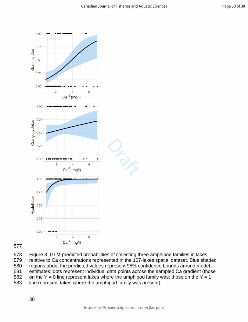
Draft

30

577

Figure 3: GLM-predicted probabilities of collecting three amphipod families in lakes 578 relative to Ca concentrations represented in the 107-lakes spatial dataset. Blue shaded 579 regions about the predicted values represent 95% confidence bounds around model 580 estimates; dots represent individual data points across the sampled Ca gradient (those 581 on the Y = 0 line represent lakes where the amphipod family was; those on the Y = 1 582 line represent lakes where the amphipod family was present). 583

Page 30 of 38

https://mc06.manuscriptcentral.com/cjfas-pubs

Canadian Journal of Fisheries and Aquatic Sciences

Draft

31

584

Figure 4: Relationship between lake-water Ca concentration and year, 19-lake temporal 585 dataset. 586

587

588

Figure 5: Relationship between amphipod abundance and year, 19-lake temporal 589 dataset. 590

Page 31 of 38

https://mc06.manuscriptcentral.com/cjfas-pubs

Canadian Journal of Fisheries and Aquatic Sciences

Draft

32

591

Figure 6: Relationship between amphipod abundance and lake-water Ca concentration, 592 19-lake temporal dataset 593

Page 32 of 38

https://mc06.manuscriptcentral.com/cjfas-pubs

Canadian Journal of Fisheries and Aquatic Sciences

Draft

33

Tables 594

Table 1: Summary of GLM statistics (presence/absence of amphipod families,107-lake 595 spatial dataset; “.pa” = denotes presence/absence data; Gamma = Gammaridae, Crang 596 = Crangonyctidae, Hyale = Hyalellidae; AIC = Akaike information criterion, SE = 597 standard error; upper and lower confidence limits for parameter estimates are provided 598 in parentheses). 599

600

601

Response Predictor Estimate SE p AIC R2

Gamma.pa Intercept -1.894 (-2.782, -1.113) 0.422 <0.01 123.62 0.112

Calcium 3.747 (1.555, 6.258) 1.187 <0.01

Crang.pa Intercept -0.043 (-0.71, 0.615) 0.336 0.9 148.597 0.009

Calcium 0.992 (-0.948, 3.073) 1.013 0.33

Hyale.pa Intercept 1.092 (-0.154, 2.457) 0.655 0.1 48.524 0.039

Calcium 8.505 (1.821, 18.135) 4.082 0.04

Page 33 of 38

https://mc06.manuscriptcentral.com/cjfas-pubs

Canadian Journal of Fisheries and Aquatic Sciences

Draft

34

Table 2: Summary of GLM statistics (abundances of amphipod families,107-lake spatial 602 dataset; Gamma = Gammaridae, Crang = Crangonyctidae, Hyale = Hyalellidae ; AIC = 603 Akaike information criterion, SE = standard error; upper and lower confidence limits for 604 parameter estimates are provided in parentheses). 605

606

607

Response Predictor Estimate SE p AIC R2

Gamma (Intercept) -8.003 (-8.913, -7.144) 0.451 <0.01 1252.2 0.24

Ca 1.11 (0.156, 2.073) 0.488 0.02

Cl 2.252 (1.037, 3.391) 0.599 <0.01

DOC 2.145 (0.594, 3.684) 0.788 <0.01

TP 0.726 (-0.225, 1.649) 0.478 0.13

pH 1.309 (0.587, 2.062) 0.376 <0.01

area 3.123 (2.444, 3.83) 0.353 <0.01

PCmed 1.51 (0.288, 2.685) 0.611 0.01

Me -0.082 (-0.613, 0.452) 0.272 0.76

Mrf -9.867 (-11.908, -8.045) 0.984 <0.01

Ms 1.96 (1.264, 2.673) 0.359 <0.01

Crang (Intercept) -5.906 (-6.851, -5.02) 0.467 <0.01 576.1 0.27

Ca 1.649 (0.424, 2.934) 0.638 <0.01

Cl 0.342 (-1.266, 1.692) 0.751 0.65

DOC 2 (0.048, 3.889) 0.981 0.04

TP -2.21 (-3.803, -0.71) 0.789 <0.01

pH 0.726 (-0.251, 1.783) 0.518 0.16

area 1.03 (0.267, 1.805) 0.392 <0.01

PCmed 0.741 (-0.515, 1.907) 0.617 0.23

Me -0.191 (-0.886, 0.496) 0.352 0.59

Mrf -1.642 (-2.633, -0.719) 0.487 <0.01

Ms -0.969 (-1.756, -0.188) 0.400 0.02

Hyale (Intercept) -2.444 (-2.673, -2.218) 0.116 <0.01 2179.2 0.29

Ca -0.342 (-0.678, -0.008) 0.171 0.05

Cl 0.661 (0.378, 0.938) 0.143 <0.01

DOC -1.26 (-1.758, -0.768) 0.253 <0.01

TP 0.218 (-0.14, 0.572) 0.182 0.23

pH 0.681 (0.366, 1) 0.162 <0.01

area 0.235 (0.013, 0.455) 0.113 0.04

PCmed -1.997 (-2.385, -1.621) 0.195 <0.01

Me 0.737 (0.558, 0.917) 0.092 <0.01

Mrf -0.87 (-1.085, -0.657) 0.109 <0.01

Ms 0.124 (-0.068, 0.317) 0.098 0.21

Page 34 of 38

https://mc06.manuscriptcentral.com/cjfas-pubs

Canadian Journal of Fisheries and Aquatic Sciences

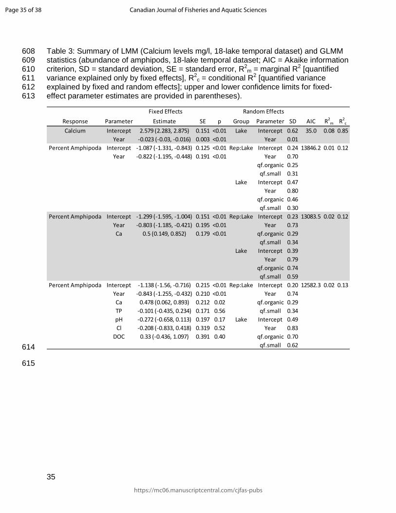
Draft

35

Table 3: Summary of LMM (Calcium levels mg/l, 18-lake temporal dataset) and GLMM 608 statistics (abundance of amphipods, 18-lake temporal dataset; AIC = Akaike information 609 criterion, SD = standard deviation, SE = standard error, R2

m = marginal R2 [quantified 610 variance explained only by fixed effects], R2

c = conditional R2 [quantified variance 611 explained by fixed and random effects]; upper and lower confidence limits for fixed-612 effect parameter estimates are provided in parentheses). 613

614

615

Fixed Effects Random Effects

Response Parameter Estimate SE p Group Parameter SD AIC R2m R2

c

Calcium Intercept 2.579 (2.283, 2.875) 0.151 <0.01 Lake Intercept 0.62 35.0 0.08 0.85

Year -0.023 (-0.03, -0.016) 0.003 <0.01 Year 0.01

Percent Amphipoda Intercept -1.087 (-1.331, -0.843) 0.125 <0.01 Rep:Lake Intercept 0.24 13846.2 0.01 0.12

Year -0.822 (-1.195, -0.448) 0.191 <0.01 Year 0.70

qf.organic 0.25

qf.small 0.31

Lake Intercept 0.47

Year 0.80

qf.organic 0.46

qf.small 0.30

Percent Amphipoda Intercept -1.299 (-1.595, -1.004) 0.151 <0.01 Rep:Lake Intercept 0.23 13083.5 0.02 0.12

Year -0.803 (-1.185, -0.421) 0.195 <0.01 Year 0.73

Ca 0.5 (0.149, 0.852) 0.179 <0.01 qf.organic 0.29

qf.small 0.34

Lake Intercept 0.39

Year 0.79

qf.organic 0.74

qf.small 0.59

Percent Amphipoda Intercept -1.138 (-1.56, -0.716) 0.215 <0.01 Rep:Lake Intercept 0.20 12582.3 0.02 0.13

Year -0.843 (-1.255, -0.432) 0.210 <0.01 Year 0.74

Ca 0.478 (0.062, 0.893) 0.212 0.02 qf.organic 0.29

TP -0.101 (-0.435, 0.234) 0.171 0.56 qf.small 0.34

pH -0.272 (-0.658, 0.113) 0.197 0.17 Lake Intercept 0.49

Cl -0.208 (-0.833, 0.418) 0.319 0.52 Year 0.83

DOC 0.33 (-0.436, 1.097) 0.391 0.40 qf.organic 0.70

qf.small 0.62

Page 35 of 38

https://mc06.manuscriptcentral.com/cjfas-pubs

Canadian Journal of Fisheries and Aquatic Sciences

Draft

36

Table 4: Trends in amphipod abundances and lake-water Ca concentrations, 18-lake 616 temporal dataset (upper and lower 95% confidence limits for slopes are provided in 617 parentheses; where confidence limits for slopes do not include zero, the sign of the 618 trend is indicated) 619

620

621

Lake Amphipod Slope Trend Ca Slope Trend

BC -0.239 (-2.011, 1.533) -0.013 (-0.027, 0.002)

BW -1.015 (-1.864, -0.165) - -0.028 (-0.043, -0.013) -

CB -0.550 (-1.373, 0.274) -0.022 (-0.037, -0.007) -

CL -0.652 (-1.464, 0.159) - -0.029 (-0.044, -0.014) -

CN -1.218 (-2.107, -0.330) -0.030 (-0.044, -0.015) -

CRDL -0.643 (-1.988, 0.703) -0.009 (-0.024, 0.006)

DE -1.030 (-1.963, -0.098) - -0.001 (-0.016, 0.013)

DO -0.453 (-1.400, 0.494) -0.003 (-0.018, 0.012)

HP 1.264 (0.443, 2.085) + -0.016 (-0.031, -0.002) -

HR -1.330 (-2.179, -0.482) - -0.046 (-0.062, -0.030) -

HY -1.512 (-2.588, -0.435) - -0.021 (-0.036, -0.006) -

PC -2.425 (-4.295, -0.555) - -0.028 (-0.042, -0.013) -

PNCR -1.233 (-2.091, -0.374) - -0.016 (-0.031, -0.001) -

RCE -0.956 (-1.851, -0.060) - -0.023 (-0.037, -0.008) -

RCM -0.344 (-1.216, 0.528) -0.030 (-0.043, -0.013) -

RDT -0.644 (-1.628, 0.341) -0.031 (-0.048, -0.014) -

WD -0.526 (-1.880, 0.828) -0.024 (-0.040, -0.008) -

YG -0.822 (-2.096, 0.451) -0.038 (-0.053, -0.022) -

Page 36 of 38

https://mc06.manuscriptcentral.com/cjfas-pubs

Canadian Journal of Fisheries and Aquatic Sciences

Draft

37

Table 5: Future Ca concentrations and amphipod abundances projected from 18-lake 622 temporal dataset ([Ca] = lake-water Ca concentration; upper and lower 95% confidence 623 limits in parentheses) 624 625

626

627

Lake

1993 - 2016

mean observed

[Ca] (mg/l)

[Ca] corresponding

with 40% reduction

from 1993-2016

mean (mg/l)

Year 40% [Ca]

reduction reached

1993 - 2016

mean observed

amphipod

abundance (%)

Predicted amphipod

abundance at

minimum simulated

[Ca] (%)

BC 2.30 1.38 2098 (2038, >2100) 43 23 (4, 70)

BW 1.93 1.16 2039 (2019, 2080) 32 14 (2, 53)

CB 1.73 1.04 2045 (2018, >2100) 16 9 (1, 42)

CL 1.78 1.07 2030 (2017, 2055) 34 18 (3, 62)

CN 1.63 0.98 2028 (2017, 2051) 23 11(2, 46)

CRDL 1.35 0.81 >2100 (2043, >2100) 16 15 (2, 59)

DE 2.68 1.61 >2100 (>2100, >2100) 32 19 (3, 64)

DO 1.90 1.14 >2100 (>2100, >2100) 31 24 (4, 70)

HP 2.63 1.58 >2100 (2046, >2100) 20 14 (2, 53)

HR 2.47 1.48 2023 (2017, 2031) 17 11 (2, 43)

HY 1.61 0.97 2035 (2017, 2077) 17 10 (1, 47)

PC 1.40 0.84 2025 (2017, 2048) 15 3 (0, 19)

PNCR 1.22 0.73 >2100 (2023, >2100) 11 9 (1, 44)

RCE 2.14 1.28 2047 (2022, >2100) 33 21 (3, 67)

RCM 2.04 1.23 2036 (2017, 2065) 34 25 (4, 72)

RDT 1.90 1.14 2029 (2017, 2050) 43 19 (3, 65)

WD 1.68 1.01 2036 (2017, 2077) 35 22 (3, 69)

YG 2.28 1.37 2026 (2017, 2037) 44 18 (3, 61)

Page 37 of 38

https://mc06.manuscriptcentral.com/cjfas-pubs

Canadian Journal of Fisheries and Aquatic Sciences

Draft

38

Electronic Supplements 628

ES#1: Datasets 629

ES#2: R Scripts 630

Acknowledgements 631

Thanks to Ron Reid and Keith Somers, who initiated the Temporal Study, and 632

oversaw it between approximately 1993 and 2008. We acknowledge contributions made 633

by Ron Ingram, Sarah Sinclair, Mark MacDougall (who collected and processed many 634

samples, and assisted with data compilation), and Johnny Su (database administrator). 635

Thanks also to the many staff of the Dorset Environmental Science Centre and students 636

of the University of Waterloo who assisted with sampling activities. 637

This research was funded by the Ontario Ministry of Environment and Climate 638

Change and a grant from the Canadian Water Network that supported development of a 639

cumulative effects monitoring framework for the Muskoka River Watershed. 640

641

642

643

644

Page 38 of 38

https://mc06.manuscriptcentral.com/cjfas-pubs

Canadian Journal of Fisheries and Aquatic Sciences

143

PART 6: SUMMARY, CONCLUSIONS AND DISCUSSION

144

Summary

A tense opposition is apparent in Earth’s boreal ecosystems. On one hand, the

boreal region has expansive natural areas and valuable resources (such as timber,

fossil fuels, minerals, fisheries, and waterfront real estate; Luke et al 2007). On the

other hand, human influence is pervasive, and threats of additional development and

resource exploitation are unrelenting (Dubé et al. 2006, Sorensen et al. 2008, Houle et

al. 2010, Seitz et al. 2011).

Cumulative effects assessment (CEA) has been viewed as a way to promote

precaution in the land use planning and development process and to facilitate

sustainability (Benson 2003, Gunn and Noble 2009, Gunn and Noble 2011); however,

its execution is frequently stalled due to a lack of clarity about what cumulative effects

assessment is and how it is best implemented (Duinker and Grieg 2006, Gunn and

Noble 2011), and because the necessary monitoring systems and cumulative effects

models are rudimentary (Duinker and Greig 2007, Ball et al. 2013).

Water is essential for life, and access to sufficient clean water is commonly

viewed as a human right (Gupta et al. 2010). Nonetheless, lakes and rivers are exposed

to (Nõges et al., 2016), and integrate effects of, many stressors (Lowell et al., 2000,

Townsend et al., 2008, Ormerod et al. 2010, Jackson et al. 2016). Indeed, several

authors have considered aquatic ecosystems to be among the most threatened

ecosystems on Earth (e.g., Schindler 2001, Carpenter et al. 2011). Given the universal

and incomparable importance of water, the quality of lake and river water, and the

biological condition of lake and river ecosystems are critical considerations for CEA.

145

The Muskoka River Watershed is a microcosm of the boreal region, and serves

as a useful case-study. In this watershed, the regional planning authority (the District

Municipality of Muskoka) and other regulatory agencies (for example Ontario’s

Ministries of Environment and Climate Change, and Natural Resources and Forestry),

have been collaborating with several academic institutions to design a cumulative

effects monitoring system and initiate a process for CEA (CWN 2015, Eimers 2016). My

intent is to provide these agencies with requisite knowledge.

The thesis begins by synthesizing a conceptual model for CEA. Subsequent

chapters describe and model lake and stream water quality, benthic community

structure, and the cumulative effects of natural environmental factors and human land-

use (urbanization and agriculture in particular). Specifically, I establish that monitoring

and modeling are essential to CEA, and clarify where these techniques fit into the CEA

process. I evaluate a series of candidate monitoring indicators by determining which

ones can be best modeled, what human and natural factors they respond to, and

whether they are sensitive enough to predict outcomes of alternative scenarios of

human activity. From this assessment, a short list of chemical and biological indicators

that should be incorporated in a regional cumulative effects monitoring program is

suggested.

Furthermore, I objectively differentiate reference and impacted conditions, either

using a criterion of no exposure to land-use stress or an empirical break-point where

stressor exposures begin to cause measurable chemical or biological effects. Such

criteria allow a series of assessment benchmarks to be reported as normal reference

ranges for biological or chemical indicators of lake or stream condition.

146

I quantify cumulative effects by modeling spatial and temporal patterns of

chemical and biological conditions across multiple gradients of natural environmental

features and human activity, which identifies a variety of ecological issues that are

relevant to CEA. As an example to illustrate the potential complexity of CEA in the

boreal region, I also explore the association between lake-water calcium concentration,

the abundance of amphipods (a freshwater crustacean with a high demand for calcium),

and local factors that mediate the calcium-amphipod relationship.

Although the focus of this thesis is on lakes and streams of the southern Boreal

Shield, its concepts and numerical methods are universal: they are equally applicable to

regions outside the Muskoka River Watershed, even though human interests and

environmental priorities may be quite different in these different localities.

147

Conclusions and Discussion

My review of the environmental-appraisal literature established 6 key themes that

encapsulate CEA and its role as a precautionary instrument for sustainability: (1)

Human wellbeing ultimately depends on the degree to which the human enterprise

conforms to the limitations of Earth’s biosphere (Wackernagel and Rees 1998,

Schnaiberg and Gould 2000). (2) Cumulative effects are combined ecosystem changes

that result from a combination of human activities and natural processes (Scherer

2011). (3) CEA is a sub-discipline of environmental impact assessment, and a

complement to municipal planning (Morgan 2012, Morrison-Saunders et al. 2014). Its

objectives are to formalize environmental values, establish a sustainable socio-

economy, improve knowledge and governance (Culhane 1990, Schultz 2012, Pope et

al. 2013), and predict the consequences of development, relative to an assessment of

present ecological condition (Dubé et al. 2003). CEA is particularly well suited to

forecasting trade-offs associated with alternative scenarios of human activity. Given

these objectives, it is best undertaken in a strategic and regional context (e.g., at the

watershed scale; Seitz et al. 2011), rather than at the conventional scale of individual

development projects (Gunn and Noble 2011). (4) As objects of its assessment, CEA

requires valued ecosystem components to be specified. These components set a

tractable scope, and focus attention on the most important environmental features and

processes (Damman et al. 1995, Canter and Ross 2010); however, objective criteria for

guiding other decisions that need to be made in the CEA process (e.g., about the spatial

or temporal bounds of the assessment, or the scope of issues to be considered) do not

exist. (5) Monitoring and adaptive management are essential strategies within CEA for

148

mitigating risks of uncertainty (Karkkainen 2002). And (6) our lack of basic knowledge

about stressors and their effects is a barrier to the development of models that assess

and predict cumulative effects (Duinker and Greig 2007).

Chapter 2 (Random Forests as Cumulative Effects Models: A Case Study of

Lakes and Rivers in Muskoka, Canada) provided two key insights: (1) Random forest

models (Breiman 2001) describe the combined and singular effects of multiple stressors

and natural factors, and can be used to evaluate the suitability of candidate indicators

for use in monitoring schemes and scenario analyses. (2) A variety of chemical and

biological measures of ecosystem condition can be modeled accurately enough, and

are sensitive enough to land-use, to be included in a cumulative effects monitoring

system and considered in futuring exercises.

In the case-study watershed, the most accurately modeled biological indicator for

lakes was an axis score from a principal coordinates analysis ordination of the relative

abundances of the benthic taxa. The best modelled biological indicator for rivers was

the relative abundance of Asellidae (a family of Isopod crustaceans, considered tolerant

of a variety of chemical pollutants; Hilsenhoff 1988, Mandaville 2002, Oguma and Klerks

2017). The most accurately modeled chemical indicator for lakes was alkalinity, and for

rivers was conductivity. In general, chemical effects were modeled more accurately than

biological effects. As a rule, biological effects were modeled more accurately for lakes

than for rivers, but chemical effects were modeled more accurately for streams than for

lakes.

149

CEA practitioners should derive some confidence in indicators, and some

optimism for the potential of futuring analyses, given that several chemical and

biological indicators were sensitive enough to detect simulated land-use changes. All 13

biological indicators that I tested (including several measures of taxonomic composition,

richness, taxa tolerances and whole-community ordination-based metrics) were capable

of detecting a doubling of urbanization in the catchment. Five of thirteen (including

measures of taxonomic composition and axis-scores from an ordination of taxa counts)

were capable of detecting a doubling of agricultural intensity in the Highway 11 Strip

physiographic region. These differences in the detectability of stressor exposures agree

with several published studies that demonstrated urbanization effects as more severe

than agricultural effects (e.g., Allan 2004, Poff et al. 2006). All indicators except

Hilsenhoff’s Family Biotic Index were better able to detect urbanization or agricultural

effects in lakes than in streams.

Chemical and biological indicators were typically influenced by a complicated

array of predictors, representing environmental factors operating at several different

spatial scales, from the immediate vicinity of the sampled location, to the riparian zone,

to the local catchment, to the cumulative catchment. Chemical, morphometric,

hydrologic and land-use/land cover predictors were more important in biological models

than geographic variables or measures of physical habitat at the sampled locations.

Measures of land-use and land cover were of greatest importance to the water-

chemistry models. Furthermore, variables describing attributes of the cumulative

catchment or physical characteristics of the sampled locations tended to be most

important in biological models; whereas those measured at the cumulative catchment

150

scale were the most important drivers of chemical indicators. These findings should be

considered when selecting monitoring indicators, and when choosing which effects to

attempt to forecast. They also serve as a reminder that one’s vantage point is

consequential: our ability to understand the relative importance of local and regional

effects on water chemistry and community structure depends both on how we define

local and regional communities, and at what scale the regulatory mechanisms operate

(Weiher et al. 2011).

My models of metric values demonstrated that random forests provide useful

insights about the performance of candidate indicators. From the perspective of metric

selection, the pseudo-R2 statistic is informative because it provides a direct measure of

predictive accuracy or explained variance. Variable importances and partial

dependencies reveal what a given metric actually indicates — i.e., they provide

information about which stressors and natural environmental factors the indicator

responds to. Such evidence is needed so that reference-site-selection and

bioassessment methods can be fine-tuned to judge ecological condition in a way that is

minimally confounded by natural variability (Mazor et al. 2016). Aside from their use in

indicator evaluations, random forest models could also be used as a basis for mapping

present or expected waterbody condition, or to hindcast reference conditions (Clapcott

et al. 2017).

Unexplained variation in my random forest models may be associated with

unmeasured environmental features, sampling error, temporal variance (mazor et al.

2016), metacommunity dynamics (Leibold et al. 2004, Heino 2012), or neutral

processes in community assembly that are inherently unpredictable (Hubbell 2001). The

151

relative contribution of these factors should continue to be an active area of

bioassessment research (Mazor et al. 2016).

A wide variety of cumulative effects were observed in the Muskoka River

Watershed, and cross-validation demonstrated the underlying models to have

reasonable generality1. These effects constitute environmental issues, and suggest

hypothetical mechanisms that are worthy of consideration in CEA. For example,

Chironomidae become more numerically dominant in lake samples as lake pH

decreases, which reinforces results from earlier studies demonstrating the

Chironomidae to be tolerant of acidification (Wiederholm and Eriksson 1977, Schindler

et al. 1985). In rivers, aquatic earthworms (the oligochaetous Clitellata) become more

abundant as the proportion of the riparian zone under urban land-cover increases

(potentially an effect of storm water and associated sedimentation), and as stream size

increases (which is consistent with predictions from the River Continuum Concept;

Vannote et al. 1980). Conductivity, alkalinity, chloride, and calcium concentrations in

lakes and rivers increase with the intensity of human land-use in their catchments,

which isn’t surprising given the typical increase in solutes that accompanies many types

of developments (Winter and Duthie 1998, Paul and Meyer 2001, Foley et al. 2005).

Likewise, models of lake total phosphorus concentrations were best informed by

drainage basin slopes, and agricultural intensity in the riparian zone, which reinforces

wetlands and farms as areas of elevated nutrient fluxes (e.g., Sims et al. 1998; Reddy

et al.1999).

1 probably owing to the random forest’s “bagging” procedure, in which numerous trees are assembled by

bootstrapping (Breimer 2001)

152

Although many of the singular effects I identified were linear (e.g. the effect of pH

on the relative abundance of lake Chironomidae), several were non-linear (e.g., effect of

catchment forest cover on total nitrogen in rivers; conductivity and lake perimeter effects

on the relative abundance of lake Chironomidae; effects of lake depth on dissolved

organic carbon). Therefore, the ability to handle non-linear responses should be

considered a compulsory feature of cumulative effects models.

The concept of the reference condition is ambiguous, and has been difficult to

“translate from theory to practice” (Pardo et al 2012), given that the allowable level of

anthropogenic impact is not clearly articulated (Stoddard et al. 2006, Pardo et al. 2012).

Onset-of-effect thresholds represent empirical break-points where effects from stressor

exposures become detectable (Utz et al. 2009). As long as reasonable criteria for

identifying thresholds can be derived2, the reference condition approach can be made

more objective by using such thresholds to differentiate reference and impacted sites. In

Chapter 3 (Onset-of-effect Thresholds and Reference Conditions: A Case Study of the

Muskoka River Watershed, Canada), I reported no biological onset-of-effect thresholds;

however, lake alkalinities and electrical conductivities, calcium, chloride, dissolved

organic carbon, total Kjeldahl nitrogen, and total phosphorus concentrations, and pH

exhibited threshold responses to road density, urbanization, or agriculture, as did

stream alkalinities, conductivities and calcium and chloride concentrations. For lakes,

thresholds were slightly more commonly detected for stressor variables measured at the

cumulative-catchment scale than at the local-catchment scale; but for streams,

thresholds were detected with approximately equal frequency for stressor variables

2 Chapter 3 proposes complementary use of random forest and TITAN assessments; however no

objective criteria for threshold identification exist.

153

measured at the two different scales. Several authors (e.g., Booth and Jackson 1997,

Brabec et al. 2002) have reported threshold responses at very low levels of stressor

exposure, and my study provides further evidence of this phenomenon. I demonstrated

onset-of-effect thresholds as low as 1% agriculture (chloride in streams), 0.0002 m/m2

road density (e.g., alkalinity and chloride in lakes) and 0.2% urbanization (alkalinity in

lakes).

When sampled locations were grouped as reference or impacted based either on

these thresholds or the default zero-stress criterion, insights about cumulative effects

from the random forests were reinforced. Impacted waterbodies had more variable

taxonomic structure and water chemistry, and had higher alkalinities and conductivities,

calcium, chloride, and phosphorus concentrations, and pH than was typical of reference

waterbodies. Furthermore, Amphipoda, Asellidae, Corixidae, Gastropoda, and

Hirudinea were more abundant, and Chironomidae were less abundant in impacted

streams than in reference streams, and insects were less abundant in impacted lakes

than in reference lakes.

Differences in means and within-group variation between the groups of reference

and impacted lakes and streams can be attributed to a combination of cumulative

effects of human activities and natural factors. It is difficult to distinguish these sources

of variation because land-uses are not dispersed evenly or randomly across

watersheds, and because the intensity and types of developments are typically

correlated with environmental features, which results in these features being unequally

154

distributed among reference and impacted groups3. Nonetheless, the degree of

interspersion between reference and impacted waterbodies (i.e., how similar their

geographic positions and natural environmental attributes are) is a critical consideration

for the design of cumulative effects monitoring programs. I found the geographic

locations and ranges of natural environmental features associated with reference and

impacted streams do substantially overlap in many cases. The two groups of streams,

for example, had similar ranges of geographic coordinates and elevations; however,

reference streams had shallower soils on average, and smaller catchment areas.

Lesser interspersion was apparent for the two groups of lakes, reference lakes being,

on average, smaller and shallower, with fewer up-gradient lakes in their drainage

networks, and shallower soils in their catchments. Imperfect interspersion of reference

and impacted sites is a common problem in the reference-condition approach (Stoddard

et al. 2006, Pardo et al. 2012), and continues to be an issue in the Muskoka River

Watershed.

I tabulated normal ranges associated with a variety of chemical and biological

indicators and environmental attributes, because these ranges are useful as

assessment benchmarks (Kilgour et al. 2017). Multiple indicators were included

because numerous indicators are required to represent the complexity of lake and

stream ecosystems (Dale and Beyeler 2001), because different indicators respond

differently to different stressors (Kilgour et al. 2004), because multiple indicators may be

relevant to the Muskoka Region’s water management goals and policies, and because

3 For example, large lakes are preferred for cottage development, relative to small lakes, and areas with

gradual land-surface slopes and deep overburden are preferred for agriculture, relative to areas with steep slopes and shallow soils

155

the degree of interspersion among reference and impacted sites is different for different

indicators. My reported normal ranges should be considered a first approximation.

Additional reference lakes and streams should be sampled, because supplementary

reference data would allow tolerance regions to be estimated more precisely. A larger

pool of reference sites would also facilitate sophisticated model-based approaches for

matching test-sites with the most appropriate set of reference sites (e.g., Norris and

Hawkins 2000).

Threshold assessments have several other practical applications besides their

use in deriving assessment benchmarks. For example, the identification of onset-of-

effect thresholds can be important for early detection and mitigation, and for setting

planning and conservation targets and limits (Utz et al. 2009, Mitchell et al. 2014).

Furthermore, hypotheses about the mechanisms behind stressor effects can be

generated by combining patterns of congruence among taxa-specific thresholds with

knowledge describing the autecology and traits of component taxa (Wagenhoff et al.

2017). Further progress on cumulative effects monitoring could be achieved by

undertaking such analyses.

Chapter 4 (Declining Amphipod Abundance is Linked to Low and Declining

Calcium Concentrations in Lakes of the South Precambrian Shield) corroborates

evidence of widespread lake-water calcium declines (e.g., Jeziorski et al. 2008),

suggests that calcium levels have reached critically low levels in some lakes (i.e.,

relative to calcium requirements reported by Cairns and Yan 2009), and forecasts an

average 57% decrease in amphipod abundances by the time calcium concentrations

156

reach their predicted minima (e.g., Watmough and Aherne 2008), which is expected to

occur in most lakes between years 2023 and 2100.

I demonstrated that lake-water calcium levels declined between 1993 and 2016

in 14 of 18 lakes, and a simultaneous reduction in amphipod abundances occurred in 8

of 18 lakes. Calcium explained 13% of the variation in amphipod abundances in this

time series, making it the most important chemical, morphometric or physical-habitat

predictor of declining amphipod abundances. Furthermore, models of amphipod

presence/absence generated from a 107-lake spatial survey demonstrated that

amphipods in the families Gammaridae and Hyalellidae are more commonly present in

lakes with high calcium concentrations than in lakes with low calcium concentrations.

Nonetheless, all three common amphipod families, Crangonyctidae, Gammaridae, and

Hyalellidae, can be found in some lakes with Ca concentrations below 1 mg/l — the

lower lethal limit inferred for Gammarus, based on laboratory bioassays (Cairns and

Yan 2009) — and none exhibited a threshold response to this critical nutrient.

The mechanics and mitigating factors of calcium limitation in amphipods could be

illuminated by more focussed surveys or experiments aimed at evaluating a series of

additional working hypotheses. First, inputs from streams or groundwater (e.g., Lottig et

al. 2011) could establish calcium-rich littoral refuges that allow amphipods to persist in

lakes with low pelagic calcium levels. Given that amphipods are also present in riverine

habitats (Peckarsky 1990) and are common in stream drift (Elliott and Corlett 1972), it is

also possible that colonization pressure from lake-inflow streams (so-called “mass

effects”, Heino 2012) could substantially mitigate population effects of Ca decline in

some lakes. Second, many environmental changes are occurring in the southern Boreal

157

Shield (Palmer et al. 2011, Yan et al. 2011, Yao et al. 2013, Palmer et al. 2014), and

stressor interactions are possible (Holmstrup et al. 2010, Altshuler et al. 2011, Fischer

et al. 2013, Rollin et al. 2017). Amphipod responses to low Ca could be strongly

mediated by temperature, food availability, food quality, or other environmental

variables. Third, lakes’ historical contexts could also be important. Short-term increases

in lake-water calcium occurred due to logging, development, acid rain (Watmough and

Aherne 2008), and local use of calcium-rich dust suppressants on some roadways

(Shapiera et al. 2012), and these increases have been followed by gradual declines;

therefore, it is possible that eco-evolutionary dynamics (e.g., Lallensack 2018) could be

important, such that populations that have experienced relatively large fluctuations are

more tolerant of Ca decline than populations that have experienced modest changes.

Fourth, a question remains about whether low-Ca toxicity can be proven experimentally

in any of the region’s lakes. For example, Pearceley Lake — the lowest-Ca lake in my

temporal dataset, where amphipods have not been collected in annual monitoring

efforts since 2004 — would be a good candidate for Ca-addition or mesocosm

experiments. Fifth, body-size differences suggest that Crangonyx, Gammarus, and

Hyalella could have different calcium requirements, and useful insights could be gained

from the relative abundances of species in these genera, which calls for more detailed

taxonomic diagnoses in routine monitoring programs.

Notwithstanding factors that mitigate low-calcium stress, should lake-water

calcium levels continue to decline as expected (i.e., Watmough and Aherne 2008), we

forecast that the relative abundances of amphipods in Precambrian Shield lakes will

decline, on average, by 57%, with many of these declines occurring before the end of

158

the 2030s. Historically amphipods have been a numerically dominant taxon in the

benthic community (during the 1993-2016 period they accounted for 28% of the counts

of littoral fauna, on average). A marked reduction in the abundances of these animals

signals a major restructuring of benthic communities, and reinforces warnings about

declining Ca levels being a threat to freshwater biota (e.g. Jeziorski et al. 2008;

Jeziorski and Smol 2016). As animals with high Ca demands (such as crustaceans and

mollusks) decline in abundance, the structural and functional effects of these changes

could propagate through food webs to substantially affect softwater boreal ecosystems

(Jeziorski and Smol 2016). Water managers should be mindful of this threat, particularly

given the range of other changes presently being observed in the watershed. Strategies

for mitigating calcium loss, or supplementing calcium in catchments (e.g., the wood-ash

proposal by Azan and Yan 2017) warrant consideration.

159

References Allan, J. D. (2004). Landscapes and riverscapes: the influence of land use on stream

ecosystems. Annu. Rev. Ecol. Evol. Syst., 35, 257-284.

Altshuler, I., Demiri, B., Xu, S., Constantin, A., Yan, N. D., & Cristescu, M. E. (2011). An

integrated multi-disciplinary approach for studying multiple stressors in freshwater

ecosystems: Daphnia as a model organism.

Azan, S. 2017. Could a residential wood ash recycling programme help solve the

calcium decline problem: insights from a Muskoka wood burner’s questionnaire.

Available from: http://friendsofthemuskokawatershed.org/wp-

content/uploads/2017/11/FMW_Report_2017-10-HATSEO-1.pdf [accessed 14

April 2018].

Ball, M., Somers, G., Wilson, J. E., Tanna, R., Chung, C., Duro, D. C., & Seitz, N.

(2013). Scale, assessment components, and reference conditions: issues for

cumulative effects assessment in Canadian watersheds. Integrated environmental

assessment and management, 9(3), 370-379.

Benson, J. F. (2003). What is the alternative? Impact assessment tools and sustainable

planning. Impact Assessment and Project Appraisal, 21(4), 261-280.

Booth, D. B., & Jackson, C. R. (1997). Urbanization of aquatic systems: degradation

thresholds, stormwater detection, and the limits of mitigation. JAWRA Journal of

the American Water Resources Association, 33(5), 1077-1090.

Brabec, E., Schulte, S., & Richards, P. L. (2002). Impervious surfaces and water quality:

a review of current literature and its implications for watershed planning. Journal of

planning literature, 16(4), 499-514.

Breiman, L. (2001). Random forests. Machine learning, 45(1), 5-32.

Cairns, A., & Yan, N. (2009). A review of the influence of low ambient calcium

concentrations on freshwater daphniids, gammarids, and crayfish. Environmental

Reviews, 17: 67-79.

Canter, L., & Ross, B. (2010). State of practice of cumulative effects assessment and

management: the good, the bad and the ugly. Impact Assessment and Project

Appraisal, 28(4), 261-268.

Carpenter, S. R., Stanley, E. H., & Vander Zanden, M. J. (2011). State of the world's

freshwater ecosystems: physical, chemical, and biological changes. Annual review

of Environment and Resources, 36, 75-99.

160

Clapcott, J. E., Goodwin, E. O., Snelder, T. H., Collier, K. J., Neale, M. W., & Greenfield,

S. (2017). Finding reference: a comparison of modelling approaches for predicting

macroinvertebrate community index benchmarks. New Zealand Journal of Marine

and Freshwater Research, 51(1), 44-59.

CWN (Canadian Water Network). 2015. Managing Cumulative Effects in the Muskoka

River Watershed: Monitoring, Research and Predictive Modeling. Available from:

http://www.cwn-rce.ca/project-library/project/managing-cumulative-effects-in-the-

muskoka-river-watershed-monitoring-research-and-predictive-modeling [accessed

16 April 2018].

Culhane, P. J. (1990). NEPA's impacts on federal agencies, anticipated and

unanticipated. Envtl. L., 20, 681.

Dale, V. H., & Beyeler, S. C. (2001). Challenges in the development and use of

ecological indicators. Ecological indicators, 1(1), 3-10.

Damman, D. C., Cressman, D. R., & Sadar, M. H. (1995). Cumulative effects

assessment: the development of practical frameworks. Impact Assessment, 13(4),

433-454.

Dubé, M. G. (2003). Cumulative effect assessment in Canada: a regional framework for

aquatic ecosystems. Environmental impact assessment review, 23(6), 723-745.

Dubé, M., Johnson, B., Dunn, G., Culp, J., Cash, K., Munkittrick, K., ... & Resler, O.

(2006). Development of a new approach to cumulative effects assessment: a

northern river ecosystem example. Environmental monitoring and assessment,

113(1-3), 87-115.

Duinker, P. N., & Greig, L. A. (2006). The impotence of cumulative effects assessment

in Canada: ailments and ideas for redeployment. Environmental management,

37(2), 153-161.

Duinker, P. N., & Greig, L. A. (2007). Scenario analysis in environmental impact

assessment: Improving explorations of the future. Environmental impact

assessment review, 27(3), 206-219.

Eimers, C.E. (2016). Cumulative effects assessment and monitoring in the Muskoka

Watershed. Canadian Water Network, Waterloo. Available from: http://www.cwn-

rce.ca/assets/End-User-Reports/Monitoring-Frameworks/Muskoka/CWN-EN-

Muskoka-2016-Web.pdf (Accessed 18 March 2018).

Elliott, J. M., & Corlett, J. (1972). The ecology of Morecambe Bay. IV. Invertebrate drift

into and from the river Leven. Journal of applied ecology, 195-205.

161

Fischer, B. B., Pomati, F., & Eggen, R. I. (2013). The toxicity of chemical pollutants in

dynamic natural systems: the challenge of integrating environmental factors and

biological complexity. Science of the Total Environment, 449, 253-259.

Foley, J. A., DeFries, R., Asner, G. P., Barford, C., Bonan, G., Carpenter, S. R., ... &

Helkowski, J. H. (2005). Global consequences of land use. science, 309(5734),

570-574.

Gunn, J. H., & Noble, B. F. (2009). Integrating cumulative effects in regional strategic

environmental assessment frameworks: lessons from practice. Journal of

environmental assessment policy and management, 11(03), 267-290.

Gunn, J., & Noble, B. F. (2011). Conceptual and methodological challenges to

integrating SEA and cumulative effects assessment. Environmental Impact

Assessment Review, 31(2), 154-160.

Gupta, J., Ahlers, R., & Ahmed, L. (2010). The human right to water: moving towards

consensus in a fragmented world. Review of European, Comparative &

International Environmental Law, 19(3), 294-305.

Heino, J. (2012). The importance of metacommunity ecology for environmental

assessment research in the freshwater realm. Biological Reviews, 88(1), 166-178.

Hilsenhoff, W. L. (1988). Rapid field assessment of organic pollution with a family-level

biotic index. Journal of the North American Benthological Society, 7(1), 65-68.

Holmstrup, M., Bindesbøl, A. M., Oostingh, G. J., Duschl, A., Scheil, V., Köhler, H. R., ...

& Gerhardt, A. (2010). Interactions between effects of environmental chemicals

and natural stressors: a review. Science of the Total Environment, 408(18), 3746-

3762.

Houle, M., Fortin, D., Dussault, C., Courtois, R., & Ouellet, J. P. (2010). Cumulative

effects of forestry on habitat use by gray wolf (Canis lupus) in the boreal forest.

Landscape ecology, 25(3), 419-433.

Hubbell, S.P. [2001] The Unified Neutral Theory of Biodiversity and Biogeography,

Monographs in Population Biol., Princeton Univ. Press, Princeton.

Jackson, M. C., Loewen, C. J., Vinebrooke, R. D., & Chimimba, C. T. (2016). Net effects

of multiple stressors in freshwater ecosystems: a meta‐analysis. Global Change

Biology, 22(1), 180-189.

Jeziorski, A., Yan, N. D., Paterson, A. M., DeSellas, A. M., Turner, M. A., Jeffries, D. S.,

... & McIver, K. (2008). The widespread threat of calcium decline in fresh waters.

science, 322(5906), 1374-1377.

162

Jeziorski, A., & Smol, J. P. (2016). The ecological impacts of lakewater calcium decline

on softwater boreal ecosystems. Environmental Reviews, 25(2), 245-253.

Karkkainen, B. C. (2002). Toward a smarter NEPA: monitoring and managing

government's environmental performance. Colum. L. Rev., 102, 903.

Kilgour, B. W., Somers, K. M., & Barton, D. R. (2004). A comparison of the sensitivity of

stream benthic community indices to effects associated with mines, pulp and

paper mills, and urbanization. Environmental Toxicology and Chemistry, 23(1),

212-221.

Kilgour, B. W., Somers, K. M., Barrett, T. J., Munkittrick, K. R., & Francis, A. P. (2017).

Testing against “normal” with environmental data. Integrated environmental

assessment and management, 13(1), 188-197.

Lallensack, R. (2018). How warp-speed evolution is transforming ecology. Nature, 554,

19-21.

Leibold, M. A., Holyoak, M., Mouquet, N., Amarasekare, P., Chase, J. M., Hoopes, M.

F., ... & Loreau, M. (2004). The metacommunity concept: a framework for multi‐

scale community ecology. Ecology letters, 7(7), 601-613.

Lottig, N. R., Stanley, E. H., Hanson, P. C., & Kratz, T. K. (2011). Comparison of

regional stream and lake chemistry: differences, similarities, and potential drivers.

Limnology and Oceanography, 56(5), 1551-1562.

Lowell, R. B., Culp, J. M., & Dubé, M. G. (2000). A weight‐of‐evidence approach for

northern river risk assessment: Integrating the effects of multiple stressors.

Environmental Toxicology and Chemistry, 19(4), 1182-1190.

Luke, S. H., Luckai, N. J., Burke, J. M., & Prepas, E. E. (2007). Riparian areas in the

Canadian boreal forest and linkages with water quality in streams. Environmental

Reviews, 15(NA), 79-97.

Mandaville, S. M. (2002). Benthic macroinvertebrates in freshwaters: taxa tolerance

values, metrics, and protocols (pp. 21-38). Nova Scotia: Soil & Water Conservation

Society of Metro Halifax.

Mazor, R. D., Rehn, A. C., Ode, P. R., Engeln, M., Schiff, K. C., Stein, E. D., ... &

Hawkins, C. P. (2016). Bioassessment in complex environments: designing an

index for consistent meaning in different settings. Freshwater Science, 35(1), 249-

271.

163

Mitchell, B. R., Tierney, G. L., Schweiger, E. W., Miller, K. M., Faber-Langendoen, D., &

Grace, J. B. (2014). Getting the message across: Using ecological integrity to

communicate with resource managers. In Application of Threshold Concepts in

Natural Resource Decision Making (pp. 199-230). Springer, New York, NY.

Morgan, R. K. (2012). Environmental impact assessment: the state of the art. Impact

Assessment and Project Appraisal, 30(1), 5-14.

Morrison-Saunders, A., Pope, J., Gunn, J. A., Bond, A., & Retief, F. (2014).

Strengthening impact assessment: a call for integration and focus. Impact

Assessment and Project Appraisal, 32(1), 2-8.

Newman, M. C., & Clements, W. (2008). Biotic and abiotic factors that regulate

communities. Ecotoxicology. A Comprehensive Treatment, Taylor and

Francis/CRC Press, Boca Raton, 379-407.

Nõges, P., Argillier, C., Borja, Á., Garmendia, J. M., Hanganu, J., Kodeš, V., ... & Birk,

S. (2016). Quantified biotic and abiotic responses to multiple stress in freshwater,

marine and ground waters. Science of the Total Environment, 540, 43-52.

Norris, R. H., & Hawkins, C. P. (2000). Monitoring river health. Hydrobiologia, 435(1), 5-

17.

Oguma, A. Y., & Klerks, P. L. (2017). Pollution-induced community tolerance in benthic

macroinvertebrates of a mildly lead-contaminated lake. Environmental Science

and Pollution Research, 24(23), 19076-19085.

Ormerod, S. J., Dobson, M., Hildrew, A. G., & Townsend, C. (2010). Multiple stressors

in freshwater ecosystems. Freshwater Biology, 55(s1), 1-4.

Palmer, M. E., Yan, N. D., Paterson, A. M., & Girard, R. E. (2011). Water quality

changes in south-central Ontario lakes and the role of local factors in regulating

lake response to regional stressors. Canadian journal of fisheries and aquatic

sciences, 68(6), 1038-1050.

Palmer, M. E., Yan, N. D., & Somers, K. M. (2014). Climate change drives coherent

trends in physics and oxygen content in North American lakes. Climatic change,

124(1-2), 285-299.

Pardo, I., Gómez-Rodríguez, C., Wasson, J. G., Owen, R., van de Bund, W., Kelly, M.,

... & Mengin, N. (2012). The European reference condition concept: a scientific

and technical approach to identify minimally-impacted river ecosystems. Science

of the Total Environment, 420, 33-42.

164

Paul, M. J., & Meyer, J. L. (2001). Streams in the urban landscape. Annual review of

Ecology and Systematics, 32(1), 333-365.

Peckarsky, B. L. (1990). Freshwater macroinvertebrates of northeastern North America.

Poff, N. L., Olden, J. D., Vieira, N. K., Finn, D. S., Simmons, M. P., & Kondratieff, B. C.

(2006). Functional trait niches of North American lotic insects: traits-based

ecological applications in light of phylogenetic relationships. Journal of the North

American Benthological Society, 25(4), 730-755.

Pope, J., Bond, A., Morrison-Saunders, A., & Retief, F. (2013). Advancing the theory

and practice of impact assessment: Setting the research agenda. Environmental

Impact Assessment Review, 41, 1-9.

Reddy, K. R., Kadlec, R. H., Flaig, E., & Gale, P. M. (1999). Phosphorus retention in

streams and wetlands: a review. Critical reviews in environmental science and

technology, 29(1), 83-146.

Rollin, M., Coulaud, R., Danger, M., Sohm, B., 526 Flayac, J., Bec, A., ... & Felten, V.

(2017). Additive effect of calcium depletion and low resource quality on Gammarus

fossarum (Crustacea, Amphipoda) life history traits. Environmental Science and

Pollution Research, 1-17.

Scherer, R. (2011). Cumulative effects: a primer for watershed managers. Streamline

Watershed Management Bulletin, 14(2), 14-20.

Schnaiberg, A., & Gould, K. A. (2000). Environment and society: The enduring conflict.

Blackburn Press.

Schultz, C. A. (2012). The US Forest Service's analysis of cumulative effects to wildlife:

a study of legal standards, current practice, and ongoing challenges on a National

Forest. Environmental Impact Assessment Review, 32(1), 74-81.

Schindler, D. W. (2001). The cumulative effects of climate warming and other human

stresses on Canadian freshwaters in the new millennium. Canadian Journal of

Fisheries and Aquatic Sciences, 58(1), 18-29.

Schindler, D. W., Mills, K. H., Malley, D. F., Findlay, D. L., Shearer, J. A., Davies, I. J.,

... & Cruikshank, D. R. (1985). Long-term ecosystem stress: the effects of years of

experimental acidification on a small lake. Science, 228(4706), 1395-1401.

Seitz, N. E., Westbrook, C. J., & Noble, B. F. (2011). Bringing science into river systems

cumulative effects assessment practice. Environmental Impact Assessment

Review, 31(3), 172-179.

165

Shapiera, M., Jeziorski, A., Paterson, A. M., & Smol, J. P. (2012). Cladoceran response

to calcium decline and the subsequent inadvertent liming of a softwater Canadian

Lake. Water, Air, & Soil Pollution, 223(5), 2437-2446.

Sims, J. T., Simard, R. R., & Joern, B. C. (1998). Phosphorus loss in agricultural

drainage: Historical perspective and current research. Journal of environmental

quality, 27(2), 277-293.

Sorensen, T., McLoughlin, P. D., Hervieux, D., Dzus, E., Nolan, J., Wynes, B., & Boutin,

S. (2008). Determining sustainable levels of cumulative effects for boreal caribou.

Journal of Wildlife Management, 72(4), 900-905.

Stoddard, J. L., Larsen, D. P., Hawkins, C. P., Johnson, R. K., & Norris, R. H. (2006).

Setting expectations for the ecological condition of streams: the concept of

reference condition. Ecological Applications, 16(4), 1267-1276.

Townsend, C. R., Uhlmann, S. S., & Matthaei, C. D. (2008). Individual and combined

responses of stream ecosystems to multiple stressors. Journal of Applied Ecology,

45(6), 1810-1819.

Utz, R. M., Hilderbrand, R. H., & Boward, D. M. (2009). Identifying regional differences

in threshold responses of aquatic invertebrates to land cover gradients. Ecological

indicators, 9(3), 556-567.

Vannote, R. L., Minshall, G. W., Cummins, K. W., Sedell, J. R., & Cushing, C. E. (1980).

The river continuum concept. Canadian journal of fisheries and aquatic sciences,

37(1), 130-137.

Wackernagel, M., & Rees, W. (1998). Our ecological footprint: reducing human impact

on the earth (Vol. 9). New Society Publishers.

Wagenhoff, A., Clapcott, J. E., Lau, K. E., Lewis, G. D., & Young, R. G. (2017).

Identifying congruence in stream assemblage thresholds in response to nutrient

and sediment gradients for limit setting. Ecological Applications, 27(2), 469-484.

Watmough, S. A., & Aherne, J. (2008). Estimating calcium weathering rates and future

lake calcium concentrations in the Muskoka–Haliburton region of Ontario.

Canadian Journal of Fisheries and Aquatic Sciences, 65(5), 821-833.

Weiher, E., D. Freund, T. Bunton, A.Stefanski, T. Lee, and S. Bentivenga. 2011.

Advances, challenges and a developing synthesis of ecological community

assembly theory. Philosophical Transactions of the Royal Society B 366: 2403-

2413.

Wiederholm, T., & Eriksson, L. (1977). Benthos of an acid lake. Oikos, 261-267.

166

Winter, J. G., & Duthie, H. C. (1998). Effects of urbanization on water quality, periphyton

and invertebrate communities in a southern Ontario stream. Canadian Water

Resources Journal, 23(3), 245-257.

Yao, H., Rusak, J. A., Paterson, A. M., Somers, K. M., Mackay, M., Girard, R., ... &

McConnell, C. (2013). The interplay of local and regional factors in generating

temporal changes in the ice phenology of Dickie Lake, south-central Ontario,

Canada. Inland Waters, 3(1), 1-14.

Yan, N. D., Leung, B., Lewis, M. A., & Peacor, S. D. (2011). The spread, establishment

and impacts of the spiny water flea, Bythotrephes longimanus, in temperate North

America: a synopsis of the special issue.