The econometrics of inequality and povertyChapter 4: Lorenz curves, the Gini coefficient and

parametric distributions

Michel Lubrano

October 2017

Contents

1 Introduction 2

2 General notions 32.1 Distributions . . . . . . . . . . . . . . . . . . . . . . . . . . . . . . . . . . .. 32.2 Densities . . . . . . . . . . . . . . . . . . . . . . . . . . . . . . . . . . . . . . 42.3 Quantiles . . . . . . . . . . . . . . . . . . . . . . . . . . . . . . . . . . . . . . 52.4 Some useful math results . . . . . . . . . . . . . . . . . . . . . . . . . . .. . . 62.5 Means and truncated means . . . . . . . . . . . . . . . . . . . . . . . . . .. . . 7

3 Lorenz curves 83.1 A partial moment function . . . . . . . . . . . . . . . . . . . . . . . . . .. . . 83.2 Properties . . . . . . . . . . . . . . . . . . . . . . . . . . . . . . . . . . . . . .83.3 A mathematical characterization∗ . . . . . . . . . . . . . . . . . . . . . . . . . . 9

4 The Gini coefficient revisited 114.1 Gini coefficient as a surface . . . . . . . . . . . . . . . . . . . . . . . .. . . . . 114.2 Gini as a covariance . . . . . . . . . . . . . . . . . . . . . . . . . . . . . . .. . 114.3 Gini as mean of absolute differences∗ . . . . . . . . . . . . . . . . . . . . . . . 124.4 S-Gini∗ . . . . . . . . . . . . . . . . . . . . . . . . . . . . . . . . . . . . . . . 13

5 Estimation of the Gini coefficient 145.1 Numerical evaluation . . . . . . . . . . . . . . . . . . . . . . . . . . . . .. . . 145.2 Inference for the Gini coefficient . . . . . . . . . . . . . . . . . . .. . . . . . . 15

6 Lorenz curve and other inequality measures∗ 166.1 Schutz or Pietra index . . . . . . . . . . . . . . . . . . . . . . . . . . . . .. . . 166.2 Other inequality measures . . . . . . . . . . . . . . . . . . . . . . . . .. . . . 16

1

7 Main parametric distributions and their properties 177.1 The Pareto distribution . . . . . . . . . . . . . . . . . . . . . . . . . . .. . . . 187.2 LogNormal distribution . . . . . . . . . . . . . . . . . . . . . . . . . . .. . . . 217.3 Singh-Maddala distribution∗ . . . . . . . . . . . . . . . . . . . . . . . . . . . . 257.4 Weibull distribution∗ . . . . . . . . . . . . . . . . . . . . . . . . . . . . . . . . 287.5 Gamma distribution∗ . . . . . . . . . . . . . . . . . . . . . . . . . . . . . . . . 307.6 Variations around the Pareto distribution∗ . . . . . . . . . . . . . . . . . . . . . 317.7 Which density should we select?∗ . . . . . . . . . . . . . . . . . . . . . . . . . 32

8 Pigou-Dalton transfers and Lorenz ordering 338.1 Lorenz ordering . . . . . . . . . . . . . . . . . . . . . . . . . . . . . . . . . .. 338.2 A numerical example . . . . . . . . . . . . . . . . . . . . . . . . . . . . . . .. 338.3 Generalized Lorenz Curve . . . . . . . . . . . . . . . . . . . . . . . . . .. . . 358.4 Lorenz Ordering for usual distributions∗ . . . . . . . . . . . . . . . . . . . . . . 35

9 Parametric Lorenz curves∗ 36

10 Exercises 3910.1 Empirics . . . . . . . . . . . . . . . . . . . . . . . . . . . . . . . . . . . . . . .3910.2 Gini coefficient . . . . . . . . . . . . . . . . . . . . . . . . . . . . . . . . .. . 3910.3 LogNormal . . . . . . . . . . . . . . . . . . . . . . . . . . . . . . . . . . . . . 3910.4 Uniform . . . . . . . . . . . . . . . . . . . . . . . . . . . . . . . . . . . . . . . 3910.5 Singh-Maddala∗ . . . . . . . . . . . . . . . . . . . . . . . . . . . . . . . . . . . 4010.6 Logistic∗ . . . . . . . . . . . . . . . . . . . . . . . . . . . . . . . . . . . . . . . 4010.7 Weibull∗ . . . . . . . . . . . . . . . . . . . . . . . . . . . . . . . . . . . . . . . 40

1 Introduction

Some authors like Sen (1976) prefer to use a discrete representation of income, which is basedon the assumption that the population is finite. Atkinson (1970) and his followers prefer tosuppose that income is a continuous variable. It implies that the population is implicitly infinite,but the sample can be finite. Discrete variables and finite population are at first easy notions tounderstand while continuous variables and infinite population are more difficult to accept. But asfar as computations and derivations are concerned, continuous variables lead to integral calculuswhich is an easy topic once we know some elementary theorems.Considering a continuousrandom variable opens the way for considering special parametric densities such as the Paretoor the lognormal which have played an important role in studying income distribution. Discretemathematics are quite complicated.

In this chapter, we have marked with an asterisk the sectionsthat can be skipped at a firstreading, because they inolved a more specialized material.

2

2 General notions

We are interesting in the income distribution. Income is supposed to be a continuous randomvariableX with cumulative distributionF (.).

2.1 Distributions

Definition 1 The distribution functionF (x) gives the proportion of individuals of the populationhaving a standard of living below or equal tox.

F is a non-decreasing function of its argumentx. We suppose thatF (0) = 0 while F (∞) = 1.F (x) gives the percentage of individual with an income belowx. We usually callp that propor-tion.

A natural estimator is obtained forF (.) by considering:

F (x) =1

n

n∑

1=1

1I(xi ≤ x).

where1I(.) is the indicator function. This estimator is easy to implement. The resulting graph ofthe density might seem discontinuous for very small sample sizes, but get rapidly smoother assoon asn > 30. So there is in general no need for non-parametric smoothing.

Let us now order the observations by increasing order from the smallest to the largest andcall x[j] the observation which has rankj. We can write the natural estimator ofF as

F (x[j]) = j/n.

It is common to callx[j] an order statistics. They will play an important role for estimation. Itwill be used for qunatiles, for Lorenz curves and so on.

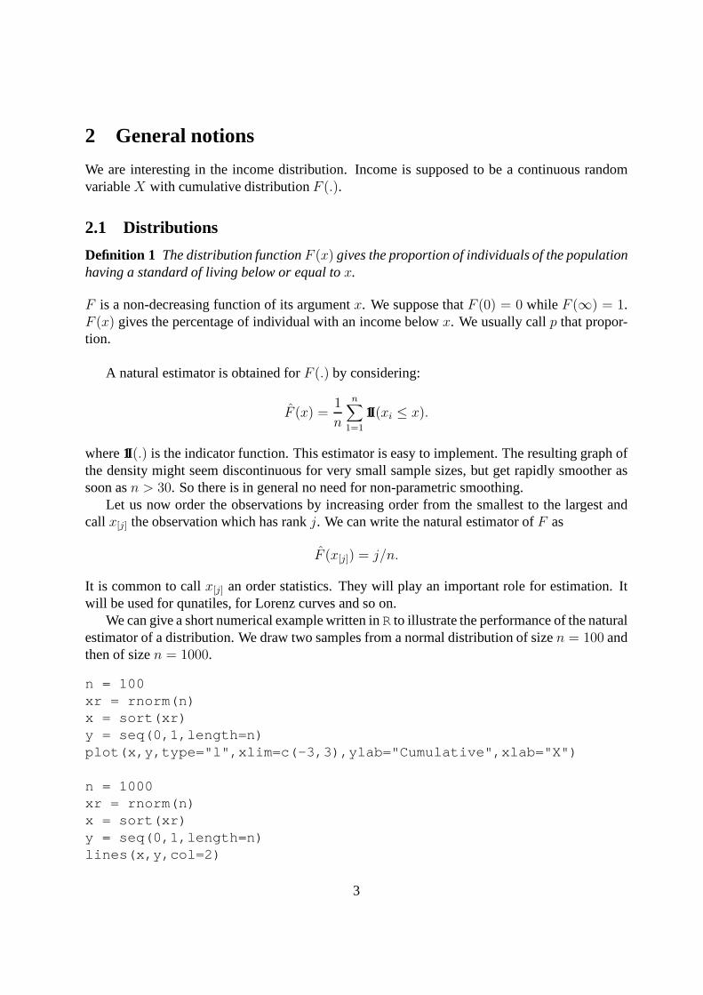
We can give a short numerical example written inRto illustrate the performance of the naturalestimator of a distribution. We draw two samples from a normal distribution of sizen = 100 andthen of sizen = 1000.

n = 100xr = rnorm(n)x = sort(xr)y = seq(0,1,length=n)plot(x,y,type="l",xlim=c(-3,3),ylab="Cumulative",xl ab="X")

n = 1000xr = rnorm(n)x = sort(xr)y = seq(0,1,length=n)lines(x,y,col=2)

3

lines(x,pnorm(x),col=3)text(-2.8,0.8,"n=1000",col=2,pos=4)text(-2.8,0.75,"n=100",col=1,pos=4)text(-2.8,0.70,"True",col=3,pos=4)

The abscises of the cumulative are obtained by ordering the draws, while the ordinates are simplyan ordered index between 0 and 1. The curve in black corresponds to the sample of size 100. It

−3 −2 −1 0 1 2 3

0.0

0.2

0.4

0.6

0.8

1.0

X

Cu

mu

lative

n=1000n=100True

Figure 1: Natural estimator of the cumulative distributionfor a Gaussian random variable

is rather rough. But the curve in red, corresponding to a sample of 1000 is perfectly smooth. Itis roughly the same as the true cumulative in green.

2.2 Densities

We shall suppose thatF is continuously differentiable so that there exist a density defined by

f(x) = F ′(x).

So, for a givenx, the value ofp such thatX < x can be defined alternatively as

p =∫ x

0f(t) dt = F (x).

4

Densities are much more complicated to estimate. There exist no natural estimator as for distri-butions, simply becauseF (.) is not differentiable. Some kind of non-parametric smoothing isneeded. Non-parametric density estimation will be detailed in a next Chapter.

If f(x) is the density, then the probability that the random variableX belongs to the interval[xk−1, xk] is given by

p(xk−1 < x < xk) ' f(xk)∆xk,

where∆xk = xk − xk−1. If the interval[a, b] is sliced inm smaller slices, then:

p(a < x < b) 'm∑

k=2

f(xk)∆xk.

If we take the limit form → ∞, we have

p(a < x < b) ' limm→∞

m∑

k=2

f(xk)∆xk =∫ b

af(x)dx.

Of course this limit exists only ifF (.) is sufficiently smooth, i.e. it has no jumps or kinks.

2.3 Quantiles

Once a distribution is given, it is always possible to compute its quantiles (this is not the casefor moments that exists only under specific conditions). Deciles are a convenient way of slicinga distribution in intervals of equal probability, each interval being of probability 1/10. Moregenerally, a quantile is a functionx = q(p) that gives the value ofx such thatF (x) = p.Quantiles are implicitly defined by the relation:

x = q(p) = F−1(p).

q(p) is thus the living standard level below which we find a proportion p of the population. Themedian of a population is the value ofx such that half of the population is belowx and half of thepopulation is abovex = q(0.50). Using quantiles is also a way to normalize the characteristicsof a population between 0 and 1. This facilitates comparisons between two populations, ignoringthus scale problems.

Quantiles are rather easy to estimate once we know the order statistics. Suppose that we havean ordered sample of sizen. The estimator of a quantile comes directly from the naturalestimatorof the distribution. Thep quantile is simply the observation that has rank[p × n]. Quantiles aredirectly estimated inRusing the instruction

quantile(x,p),

wherex is a vector containing the sample andp the level of the quantile.Piketty (2000) in his book on the history of high incomes in France makes an extensive use

of quantiles to study the French income distribution and particularly its right tail concerninghigh incomes. High incomes concern the last decile, which meansq0.90. That decile however

5

cover a variety of situations where wages, mixed incomes andcapital incomes have a varyingimportance. The intervalq0.90 − q0.95 concerns what he calls the middle class, formed mainlyby salaried executives, which thus in fact corresponds moreto the higher middle class. Theintervalq0.95 − q0.99 is the upper middle class, formed mainly by holder of intermediate incomeslike layers, doctors. The really rich persons correspond tothe last centileq0.99 and over. Itcorresponds to holders of capital income.

Defining social classes using quantiles is a very hazardous project. The poverty line can bedefined as 50% of the median. However, this does not correspond to a precise quantile. In theirpaper about inequality in China, Piketty et al. (2017) prefer to speak about the 50% bottom whichthey implicitly consider as being the poor class, the top 10%which correspond to the rich classwhile the remaining 40% represents the middle incomes.

2.4 Some useful math results

Three main rules are important to understand the next comingcalculations:

1. Integration by parts. It comes from the rule giving the derivative of a product of twofunctions ofx, u(x) andv(x):

(uv)′ = u′v + uv′.

Let us take the integral of this expression.

uv =∫

u′v du+∫

uv′ dv.

We deduce the integration by part formula by simply rearranging the terms:∫

u′v du = uv −∫

uv′ dv.

2. Compound derivatives.∂f(u(x))

∂x= f ′(u(x))u′(x).

3. Change of variable and densities. Let x ∼ f(x) and a transformationy = h(x) withinversex = h−1(y)g(y). Then the density ofy is given by:

φ(y) = |J(x → y)|f(h−1(y)),

whereJ is the absolute value of the Jacobian of the transformation

J(x → y) = |∂xi/∂yi|.

4. Change of variable and integrals. Consider the integral∫ b

af(x) dx

and the change of variablex = h(u)with reciprocalu = h−1(x). Then the original integralcan be expressed as

∫ b

af(x) dx =

∫ h−1(b)

h−1(a)f [h(u)] h′(u) du.

6

2.5 Means and truncated means

We are now going to investigate the properties of partial means. As a by-product, we shall obtainuseful formulae to define the Lorenz curve in the next subsection. We thus start from an incomedistribution with continuous densityf(x). The average standard of living in the total populationis given by the total mean:

µ =∫ ∞

0xdF (x) =

∫ ∞

0xf(x)dx.

We now consider a thresholdz and the population which is below that threshold, sometimesthepopulation over that threshold. We can compute the average standard of living of the first group,the one which is belowz. This is especially interesting for computing certain poverty indices.This is equivalent to the expectation of a truncated distribution, defined as:

µ1 =

∫ z

0xf(x)dx

F (z).

For z → ∞, we recover the mean income of the population asF (∞) = 1. Using integration byparts withu = x andv′ = f(x), we can rewrite the integral in the numerator as:

∫ z

0xf(x)dx = [xF (x)]z0 −

∫ z

0F (x)dx

= zF (z)−∫ z

0F (x)dx.

Noting thatz =∫ z

0dx, it comes that:

µ1 =

∫ z

0xf(x)dx

F (z)=∫ z

0

[

1− F (x)

F (z)

]

dx.

Incidently, if we now letz tend to infinity, we arrive at an alternative expression for the the mean:

µ =∫ ∞

0[1− F (x)]dx.

Note also that another expression of the mean can be obtainedas follows, using the quantiles.Let us start from:

µ =∫ ∞

0xf(x)dx.

By the change of variablex = F−1(p) andp = F (x), we havedp = f(x)dx and thus:

µ =∫ ∞

0xf(x)dx =

∫ 1

0F−1(p)dp =

∫ 1

0q(p)dp.

This expression will be used for explaining the Lorenz curve.

7

3 Lorenz curves

The Lorenz curve is a graphical representation of the cumulative income distribution. It showsfor the bottomp1% of households, what percentagep2% of the total income they have. Thepercentage of households is plotted on thex−axis, the percentage of income on they−axis. Itwas developed by Max O. Lorenz in 1905 for representing inequality in the wealth distribution.As a matter of fact, ifp1 = p2, the Lorenz curve is a straight line which says for instance that50% of the households have 50% of the total income. Thus the straight line represents perfectequality. And any departure from this 45◦ line represents inequality.

3.1 A partial moment function

The standard definition of the Lorenz curve is in term of two equations. First, one has to deter-mine a particular quantile, which means solving forz the equation:

p = F (z) =∫ z

0f(t)dt,

and then write:

L(p) =1

µ

∫ z

0t f(t) dt.

So the Lorenz curve is an unscaled partial moment function. Unscaled, because it is not dividedby F (z).

A notation popularized by Gastwirth (1971) used the fact that z = F−1(p) to write the Lorenzcurve in a direct way, using a change of variable:

L(p) =1

µ

∫ p

0q(t) dt =

1

µ

∫ p

0F−1(t) dt.

Alternatively, using the relationµ =∫ 10 q(t) dt, we can have another writing:

L(p) =

∫ p

0q(t) dt

∫ 1

0q(t) dt

.

The numerator sums the incomes of the bottomp proportion of the population. The denominatorsums the incomes of all the population.L(p) thus indicates the cumulative percentage of totalincome held by a cumulative proportionp of the population, when individuals are ordered inincreasing income values.

3.2 Properties

The Lorenz curve has several interesting mathematical properties.

1. It is entirely contained into a square, becausep is defined over [0,1] andL(p) is at valuealso in [0,1]. Both thex−axis and they−axis are percentages.

8

2. The Lorenz curve is not defined isµ is either 0 or∞.

3. If the underlying variable is positive and has a density, the Lorenz curve is a continuousfunction. It is always below the 45◦ line or equal to it.

4. L(p) is an increasing convex function ofp. Its first derivative:

dL(p)

dp=

q(p)

µ=

x

µwith x = F−1(p)

is always positive as incomes are positive. And so is its second order derivative (convexity).The Lorenz curve is convex inp, since asp increases, the new incomes that are beingadded up are greater than those that have already been counted. (Mathematically, a curveis convex when its second derivative is positive).

5. The Lorenz curve is invariant with positive scaling.X andcX have the same Lorenz curve.

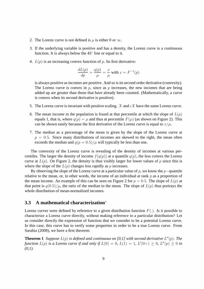
6. The mean income in the population is found at that percentile at which the slope ofL(p)equals 1, that is, whereq(p) = µ and thus at percentileF (µ) (as shown on Figure 2). Thiscan be shown easily because the first derivative of the Lorenzcurve is equal tox/µ.

7. The median as a percentage of the mean is given by the slope of the Lorenz curve atp = 0.5. Since many distributions of incomes are skewed to the right, the mean oftenexceeds the median andq(p = 0.5)/µ will typically be less than one.

The convexity of the Lorenz curve is revealing of the densityof incomes at various per-centiles. The larger the density of incomef(q(p)) at a quantileq(p), the less convex the Lorenzcurve atL(p). On Figure 2, the density is thus visibly larger for lower values ofp since this iswhere the slope of theL(p) changes less rapidly asp increases.

By observing the slope of the Lorenz curve at a particular value ofp, we know thep−quantilerelative to the mean, or, in other words, the income of an individual at rankp as a proportion ofthe mean income. An example of this can be seen on Figure 2 forp = 0.5. The slope ofL(p) atthat point isq(0.5)/µ, the ratio of the median to the mean. The slope ofL(p) thus portrays thewhole distribution of mean-normalized incomes.

3.3 A mathematical characterization∗

Lorenz curves were defined by reference to a given distribution functionF (.). Is it possible tocharacterize a Lorenz curve directly, without making reference to a particular distribution? Letus consider directly the expression of function that we consider to be a potential Lorenz curve.In this case, this curve has to verify some properties in order to be a true Lorenz curve. FromSarabia (2008), we have a first theorem:

Theorem 1 SupposeL(p) is defined and continuous on [0,1] with second derivativeL′′(p). ThefunctionL(p) is a Lorenz curve if and only ifL(0) = 0, L(1) = 1, L′(0+) ≥ 0, L′′(p) ≥ 0 in(0,1).

9

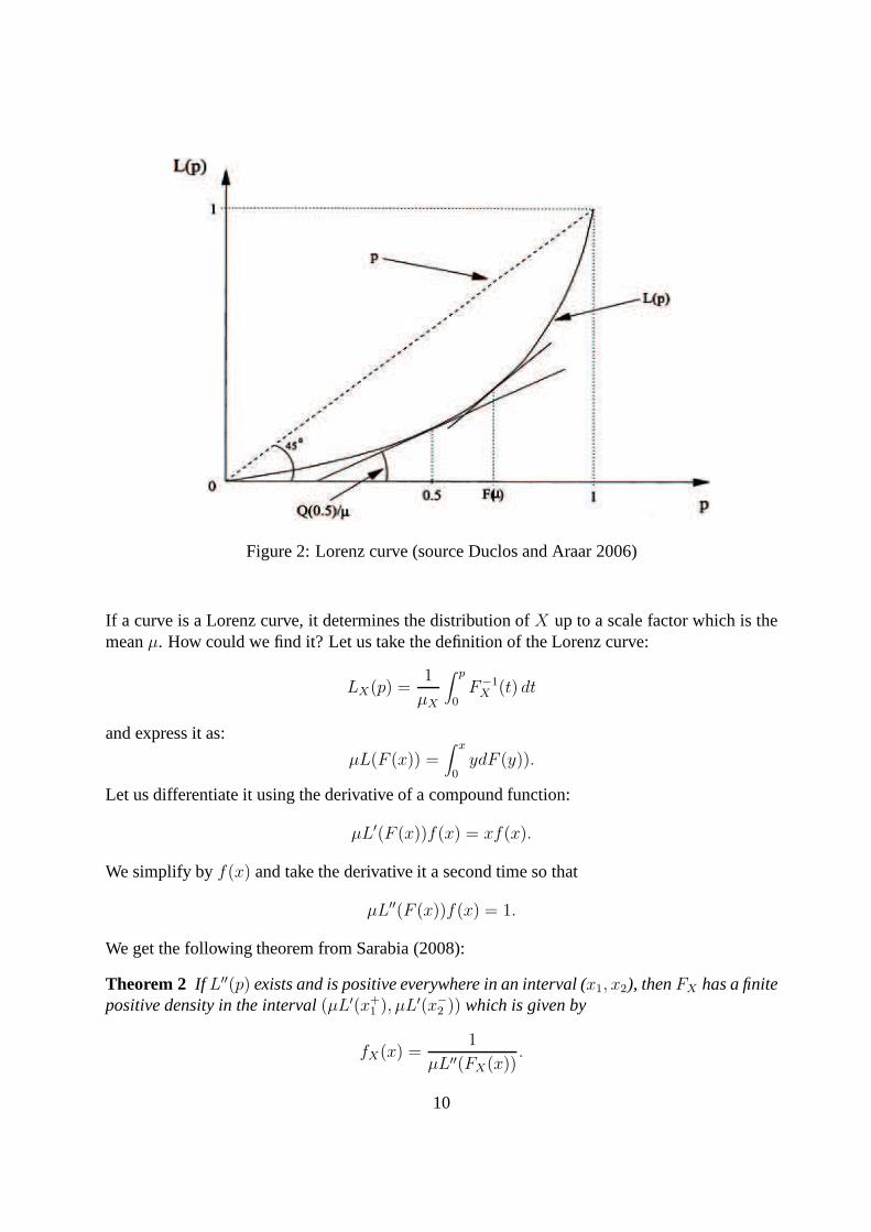
Figure 2: Lorenz curve (source Duclos and Araar 2006)

If a curve is a Lorenz curve, it determines the distribution of X up to a scale factor which is themeanµ. How could we find it? Let us take the definition of the Lorenz curve:

LX(p) =1

µX

∫ p

0F−1X (t) dt

and express it as:

µL(F (x)) =∫ x

0ydF (y)).

Let us differentiate it using the derivative of a compound function:

µL′(F (x))f(x) = xf(x).

We simplify byf(x) and take the derivative it a second time so that

µL′′(F (x))f(x) = 1.

We get the following theorem from Sarabia (2008):

Theorem 2 If L′′(p) exists and is positive everywhere in an interval (x1, x2), thenFX has a finitepositive density in the interval(µL′(x+

1 ), µL′(x−

2 )) which is given by

fX(x) =1

µL′′(FX(x)).

10

4 The Gini coefficient revisited

The Gini coefficient can be written in many different forms. In this section, we shall see how topass from the standard definition of the Gini as a surface to its various expressions (covariance,mean of absolute difference). We shall use the surveys of Yitzhaki (1998) and of Xu (2003),using however a simplification. We shall suppose that the mean of F exists. As a consequence:

limt→0

tF (t) = limt→∞

t(1− F (t)) = 0,

which means that both limits exists, which simplifies greatly the computation of some integralswhen considering an infinite bound.

4.1 Gini coefficient as a surface

If everybody had the same income, the cumulative percentageof total income held by any bottomproportionp of the population would also bep. The Lorenz curve would then beL(p) = p:population shares and shares of total income would be identical. A useful informational contentof a Lorenz curve is thus its distance,p − L(p), from the line of perfect equality in income.Compared to perfect equality, inequality removes a proportion p − L(p) of total income fromthe bottom100 · p% of the population. The larger that “deficit”, the larger the inequality ofincome. There is thus an interest in computing the average distance between these two curves orthe surface between the diagonalp and the Lorenz curveL(p). We know that the Lorenz curve iscontained in the unit square having a normalized surface of 1. The surface of the lower triangle is1/2. If we want to obtain a coefficient at values between 0 and 1, we must take twice the integralof p− L(p), i.e.:

G = 2∫ 1

0(p− L(p)) dp = 1− 2

∫ 1

0L(p)dp,

which is nothing but the usual Gini coefficient. Xu (2003) gives a good account of the algebra ofthe Gini index. We have given above an interpretation of the Gini index as a surface. The initialdefinition we gave was in term of a mean of absolute differences in the previous chapter. Thereare other formula too. All of these formula are equivalent. We have to prove this. A large surveyof the literature can also be found in the articleGini coefficientof Wikipedia.

4.2 Gini as a covariance

Let us us start from the above definition of the Gini coefficient and use integration by parts withu′ = 1 andv = L(p). Then

G = 1− 2∫ 1

0L(p)dp

= 1− 2 [pL(p)]10 + 2∫ 1

0pL′(p) dp

= −1 + 2∫ 1

0pL′(p) dp.

11

We are then going to apply a change of variablep = F (y) and use the fact proved above thatL′(p) = y/µ. We have

G =2

µ

∫ ∞

0yF (y)f(y)dy− 1 =

2

µ

[∫ ∞

0yF (y)f(y)dy− µ

2

]

.

This formula opens the way to an interpretation of the Gini coefficient in term of covariance as

Cov(y, F (y)) = E(yF (y))− E(y)E(F (y)).

Using this definition, we have immediately that

G =2

µCov(y, F (y)),

which means thatthe Gini coefficient is proportional to the covariance between a variable and itsrank. The covariance interpretation of the Gini coefficient openthe way to numerical evaluationusing a regression.

Meanwhile, noting that Cov(y, F (y)) =∫

y(F (y)− 1/2)dF (y), using integration by parts,we get

Cov(y, F (y)) =1

2

∫

F (x)[1− F (x)]dx,

so that we arrive at the integral form

G =1

µ

∫

F (x)[1− F (x)]dx.

We can remark thatF (x)(1−F (x)) is largest atF (x) = 0.5, which explains why the Gini indexis often said to be most sensitive to changes in incomes occurring around the median income.

The above integral form can also be written as

G = 1− 1

µ

∫

[1− F (x)]2dx.

We shall prove this equivalence by considering the last interpretation of the Gini which is thescaled mean of absolute differences.

4.3 Gini as mean of absolute differences∗

The initial definition of the Gini coefficient is the mean of the absolute differences divided bytwice the mean. Ify andx are two random variables of the same distributionF , this definitionimplies

IG =1

2µ

∫ ∞

0

∫ ∞

0|x− y|dF (x)dF (y).

As F (x) and1− F (x) are simply the proportions of individuals with incomes below and abovex, integrating the product of these proportions across all possible values ofx gives again the Gini

12

coefficient, in its form1µ

∫

F (x)[1− F (x)]dx. If we decide to proceed step by step, we first notethat|x− y| = (x+ y)− 2min(x, y), so that the expectation of this absolute difference is

∆ = E|x− y| = 2µ− 2E(min(x, y)).

To compute the last expectation, we need the distribution ofthe Min of two random variableshaving the same distribution. We know or we can show that it isequal to1− (1−F (y))2, whileits derivative is−d(1− F (y). So that

∆ = 2µ+ 2∫ ∞

0y d(1− F (y))2.

The last integral can be transformed using integration by parts withu = y andv = (1− F (y))2:∫ ∞

0y d(1− F (y))2 =

[

y(1− F (y))2]∞

0−∫

[1− F (y)]2dy.

So that we get the integral form of the Gini

IG =∆

2µ= 1− 1

µ

∫

[1− F (x)]2dx,

because the first right hand term is zero.

4.4 S-Gini∗

We underlined that the Gini coefficient was very sensitive tochanges in the middle of the incomedistribution. A generalization of the Gini coefficient, obtained by adding a aversion for inequalityparameter as in the Atkinson index, was proposed in the literature by Donaldson and Weymark(1980) and other papers following this contribution. Starting from

G = −2Cov(y

µ, 1− F (y)),

the S-Gini is found by introducingα so as to modify the shape of the income distribution

G = −αCov(y

µ, (1− F (y))α−1).

Forα = 2, of course, we recover the usual Gini index. With a value ofα greater than 2, a greaterweight is attached to low incomes.

We can run a small experiment, generatingn = 1000 observations of a lognormal distributionand then computing the Gini according to the above formula, with various values ofα. We thencompare the result to the Gini computed using the usual formula corresponding toα = 2.

n = 10000x = sort(rlnorm(n))y = seq(0,1,length=n)for (alpha in c(1.2,2,3,4)){

g = -alpha * cov(x/mean(x),(1-y)ˆ(alpha-1))cat("Gini = ",g," alpha = ",alpha,"\n")}

Gini(x)

13

Table 1: Computing theα-Giniusing the empirical cumulative distribution

α α-Gini Usual Gini1.2 0.2077537 -2.0 0.5288477 0.52779053.0 0.6692843 -4.0 0.7362263 -

For α = 1, the modified Gini is equal to zero. Forα = 2, this method based on the empiricalcovariance is only approximate. In small samples, the difference can be substantial. Forn = 100,the covariance method givesG = 0.5413686, while the correct methods givesG = 0.5305954.

5 Estimation of the Gini coefficient

5.1 Numerical evaluation

The definition of the Gini coefficient in term of the mean of absolute differences yield severalways of estimating it, without any assumption on the shape ofF . The direct approach using adouble summation is not feasible. We have first to order the observations to compute the orderstatisticsx[i]. Several methods were proposed in the literature:

• Deaton (1997) in his book orders the observations and proposes to use

G =n+ 1

n− 1− 2

n(n− 1)µ

∑

(n+ 1− i)x[i].

Note that this formula points out that there aren(n− 1) distinct pairs.

• Sen (1973) uses a slight simplification of this with

G =n+ 1

n− 2

n2µ

∑

(n + 1− i)x[i].

• The interpretation of the Gini coefficient in term of covariance between the variable andits rank implies that a simple routine can be used

G =2

nµCov(y[i], i).

For the covariance approach, we note that the mean of the ranks is given by

i =1

n

∑

i =n+ 1

2.

14

So the covariance is estimated by

Cov(i, y[i]) =1

n

∑

(i− i)y[i] =1

n

∑

i y[i] −n + 1

2µ,

and the Gini coefficient is obtained as:

G =2

n2µ

∑

i y[i] −n + 1

n,

which is the formula of Sen (1973).

5.2 Inference for the Gini coefficient

The main question is to find a standard deviation for the Gini coefficient. This is not an easy taskbecause the observations are ordered and thus are not independent. We can find essentially twomethods in the recent literature.

Giles (2004) found that the Gini can be estimated as

IG =2θ

n− n + 1

n, (1)

whereθ is the OLS estimate ofθ in the weighted regression

i√x[i] = θ

√x[i] + ui

√

x[i]. (2)

wherex[i] is an order statistics andi its rank. An appropriate standard error for the Gini coefficientis then

SE(IG) =2√

Var(θ)

n. (3)

This estimation is biased because the usual regression assumptions are not verified in the aboveregression. For instance the residuals are dependent.

Davidson (2009) gives an alternative expression for the variance of the Gini which is notbased on a regression, but simply on the properties of the empirical estimate ofF (x). If we noteIG the numerical evaluation of the sample Gini, we have:

ˆV ar(IG) =1

(nµ)2∑

(Zi − Z)2, (4)

whereZ = (1/n)∑n

i=1 Zi is an estimate ofE(Zi) and

Zi = −(IG + 1)x[i] +2i− 1

nx[i] −

2

n

i∑

j=1

x[j].

This is however an asymptotic result which is general gives lower values than those obtained withthe regression method of Giles. Small sample results can be obtained if we adjust a parametricdensity fory and use a Bayesian approach.

15

6 Lorenz curve and other inequality measures∗

Simple summary measures of inequality can readily be obtained from the graph of a Lorenzcurve. The share in total income of the bottomp proportion of the population is given byL(p);the greater that share, the more equal is the distribution ofincome. Analogously, the share intotal income of the richestp proportion of the population is given by1 − L(p); the greater thatshare, the more unequal is the distribution of income.

6.1 Schutz or Pietra index

An interesting but less well-known index of inequality is given by the Pietra index. What is theproportion of total income that would be needed to be reallocated across the population in orderto achieve perfect equality. This proportion is given by themaximum value ofp − L(p), whichis attained where the slope ofL(p) of the Lorenz curve is 1 (i.e., atL(p = F (µ))). It is thereforeequal to

F (µ)− L(F (µ)).

This index is called theSchutzcoefficient in Duclos and Araar (2006), but is also known underthe name of the Pietra index. In a stricter mathematical framework and following Sarabia (2008),the Pietra index is defined as the maximal deviation between the Lorenz curve and the egalitarianline

PX = max0≤p≤1

{p− LX(p)}.

If we assume thatF is strictly increasing on its support, the functionp − LX(p) will be dif-ferentiable everywhere on(0, 1) and its maximum will be reached when its first derivative inp

1− F−1(x)/µ

is zero, that is, whenx = F (µ). The value ofp− LX(p) at this point is given by

PX = F (µ)− 1

µ

∫ F (µ)

0[µ− F−1(t)]dt =

1

2µ

∫ ∞

0|t− µ|dF (t).

Consequently

PX =E|X − µ|

2µ,

which is an alternative formula for the Pietra index.

6.2 Other inequality measures

It is possible also to give a formulation of the Atkinson index and of the Entropy index as trans-formations of the Lorenz curve. We first give the expression of these two indices whenX is acontinuous random variable.

16

The Atkinson inequality indices are defined as

IA(ε) = 1−[∫ ∞

0(x/µ)1−ε dF (x)

]1/(1−ε)

, ε > 0,

whereε is the parameter that controls inequality aversion. The limiting caseε → 1 is

IA(1) = 1− 1

µexp

{∫ ∞

0log(x)dF (x)

}

.

The family of generalized entropy indices is

IG(c) =1

c(c− 1)

∫ ∞

0[(x/µ)c − 1]dF (x), c 6= 0, 1

The two particular cases obtained forc = 0 andc = 1 are

IG(0) =∫ ∞

0log(µ/x) dF (x),

andIG(1) =

∫ ∞

0(x/µ) log(x/µ) dF (x).

These two indices can be written in terms of the Lorenz Curve.We have for the Atkinsonindex

IA(ε) = 1−{∫ 1

0[L′

X(p)]1−ε dp

}1/(1−ε

, ε > 0.

For the generalized entropy index:

IG(c) =1

c(c− 1)

∫ 1

0{[L′

X(p)]c − 1}dp, c 6= 0, 1.

These formulas allow these indices to be obtained directly from the Lorenz curve without thenecessity of knowing the underlying cumulative distribution function.

7 Main parametric distributions and their properties

Several densities have been proposed in the literature to model the income distribution. Of courseall these densities are defined for a positive support. The most simple distributions, and conse-quently the widely used ones are the Pareto and the log-normal. These distributions have twoparameters. The gamma and the Weibull are also two parameterdistributions. In order to fitbetter the tails, three parameters distributions were proposed. We shall examine the mainly theSingh-Maddala distribution. We must note that all these densities are uni-modal. Four parameterdensities were proposed in the literature, without solvingthe question of multi-modality. At thisstage, mixture of simple distributions offer more flexibility without having an overwhelming costin term of parsimony.

17

7.1 The Pareto distribution

Pareto (1897) observed that in many populations the income distribution was one in which thenumber of individuals whose income exceeded a given levelx could be approximated byCxα forsome choice ofC andα. More specifically, he observed that such an approximation seemed to beappropriate for large incomes, i.e. forx above a certain threshold. If one, for various values ofx,plots the logarithm of the income level against the number ofindividuals whose income exceedsthat level, Pareto’s intuition suggests that an approximately linear plot will be encountered.

The important role of the Pareto laws in the study of income and other size distributions issomewhat comparable to the central role played by the normaldistribution in many experimentalsciences. In both settings, plausible stochastic arguments can be advanced in favour of the mod-els, but probably the deciding factor is that the models are analytically tractable and do seem toadequately fit observed data in many cases.

A random variableX follows a Pareto distribution if its survival function is

F (x) = P (X > x) =(

x

xm

)−α

, x > xm.

The use of the survival function comes from the intuitive characterization of the Pareto. Thecumulative function is simply1− F which implies

F (x) = P (X < x) = 1−(

x

xm

)−α

.

The density is obtained by differentiation

f(x) = αxαmx

−α−1, x > xm.

Moments are given in Table 7. We can already see that this density has a special shape. It is

Table 2: Moments of the Pareto distributionparameters value domainscale xm xm > 0shape α α > 0support x ∈ [xm; +∞)

median xmα√2

mode xm

mean xmα

α− 1 α > 1

variance x2m

α(α− 1)2(α− 2)

α > 2

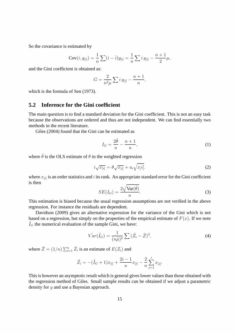
always decreasing. So it is valuable only to model high or medium incomes. Its moments arerestricted to exist only for certain values ofα. This is the price to pay for its long tails. In Figure3, we give the graph of the density forxm = 1 and various plausible values ofα. The Gini index(see Table 4 for its expression) is very sensitive to the value ofα. Table 3 shows that the most

18

1.0 1.5 2.0 2.5 3.0

0.0

0.5

1.0

1.5

2.0

2.5

3.0

x

y

alpha=1

alpha=2

alpha=3

Figure 3: Pareto density

Table 3: Gini and Pietra indices for the Paretoα 1.2 1.5 2.0 2.5 3.0 3.5Gini 0.71 0.50 0.33 0.25 0.20 0.17Pietra 0.58 0.39 0.25 0.19 0.15 0.12

plausible values of the Gini correspond to the very small rangeα ∈ [2, 2.5].The tails of the Pareto distribution have an interesting property which is nice for an empirical

test. On a log-log graph, the tail of the Pareto distributionis a straight line as

log(Pr(X ≥ x)) = α log(xm)− α log(x).

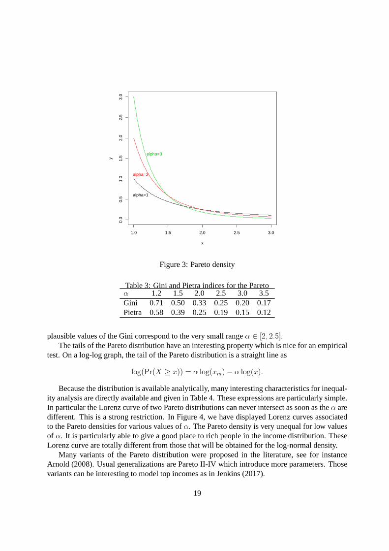
Because the distribution is available analytically, many interesting characteristics for inequal-ity analysis are directly available and given in Table 4. These expressions are particularly simple.In particular the Lorenz curve of two Pareto distributions can never intersect as soon as theα aredifferent. This is a strong restriction. In Figure 4, we havedisplayed Lorenz curves associatedto the Pareto densities for various values ofα. The Pareto density is very unequal for low valuesof α. It is particularly able to give a good place to rich people inthe income distribution. TheseLorenz curve are totally different from those that will be obtained for the log-normal density.

Many variants of the Pareto distribution were proposed in the literature, see for instanceArnold (2008). Usual generalizations are Pareto II-IV which introduce more parameters. Thosevariants can be interesting to model top incomes as in Jenkins (2017).

19

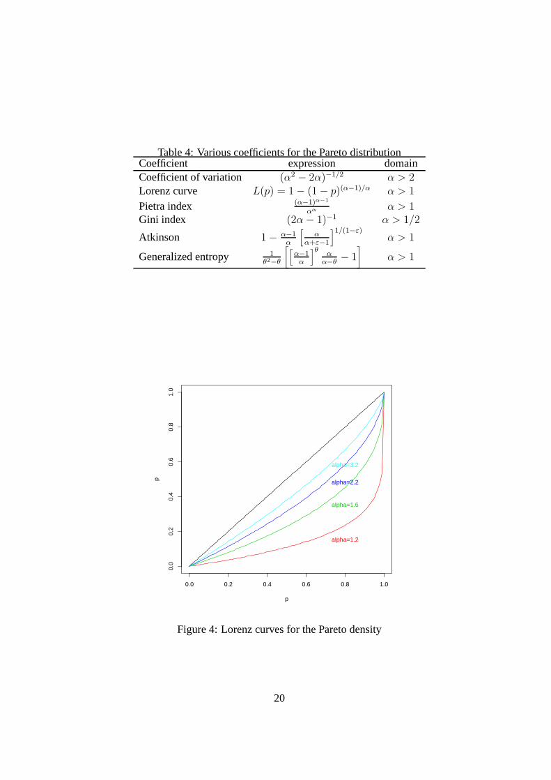
Table 4: Various coefficients for the Pareto distributionCoefficient expression domainCoefficient of variation (α2 − 2α)−1/2 α > 2Lorenz curve L(p) = 1− (1− p)(α−1)/α α > 1

Pietra index (α−1)α−1

αα α > 1Gini index (2α− 1)−1 α > 1/2

Atkinson 1− α−1α

[

αα+ε−1

]1/(1−ε)α > 1

Generalized entropy 1θ2−θ

[

[

α−1α

]θα

α−θ− 1

]

α > 1

0.0 0.2 0.4 0.6 0.8 1.0

0.0

0.2

0.4

0.6

0.8

1.0

p

p

alpha=1.2

alpha=1.6

alpha=2.2

alpha=3.2

Figure 4: Lorenz curves for the Pareto density

20

Pareto and more generally power function distributions canappear in a variety of context thatare nicely summarized in Mitzenmacher (2004). For instanceChampernowne (1953) considersa minimum incomexm and then breaks income and small intervals with bounds defined asxmγ

j

with γ > 1. Over each time step, An individual can move from classi to classj with a probabilitypij that depends only on the value ofj − i. Champernowne (1953) shows that the equilibriumdistribution is a Pareto. In fact, a Pareto is obtained in a multiplicative process with a minimumbound.

Lp = function(p,alpha) {1-(1-p)ˆ((alpha-1)/alpha)}p = seq(0,1,0.01)plot(p,p,type="l")lines(p,Lp(p,1.2),col=2)lines(p,Lp(p,1.6),col=3)lines(p,Lp(p,2.2),col=4)lines(p,Lp(p,3.2),col=5)text(0.8,0.15,"alpha=1.2",col=2)text(0.8,0.35,"alpha=1.6",col=3)text(0.8,0.48,"alpha=2.2",col=4)text(0.8,0.58,"alpha=3.2",col=5)

7.2 LogNormal distribution

The log-normal density is convenient for modelling small tomedium range incomes. A randomvariableX has a log normal distribution if its logarithmlogX has a normal distribution. IfY isa random variable with a normal distribution, thenX = exp(Y ) has a log-normal distribution;likewise, ifX is log-normally distributed, thenY = logX is normally distributed.

Let us suppose thaty is N(µ, σ2) and let us consider the change of variablex = exp y. TheJacobian of the transformation fromy to x is given by:

J(y → x) =∂y

∂x=

∂ log x

∂x=

1

x.

So, the probability density function of a log-normal distribution is:

fX(x;µ, σ) =1

xσ√2π

exp−(ln x− µ)2

2σ2, x > 0.

The cumulative distribution function has no analytical form and requires an integral evaluation:

FX(x;µ, σ) =1

2erfc

[

− ln x− µ

σ√2

]

= Φ

(

ln x− µ

σ

)

,

where erfc is the complementary error function, andΦ is the standard normal cdf. However,these integrals are easy to evaluate on a computer and built-in functions are standard.

21

The moment are easily obtained as functions ofµ andσ. If X is a log-normally distributedvariable, its expected value, variance, and standard deviation are

E[X ] = eµ+1

2σ2

,

Var[X ] = (eσ2 − 1)e2µ+σ2

,

s.d[X ] =√

Var[X ] = eµ+1

2σ2√eσ2 − 1.

Equivalently, the parametersµ andσ can be obtained if the values of the mean and the varianceare known:

µ = ln(E[X ])− 12ln(

1 + Var[X]

E[X]2

)

,

σ2 = ln

(

1 +Var[X ]E[X ]2

)

.

The mode is:Mode[X ] = eµ−σ2

.

The median is:Med[X ] = eµ.

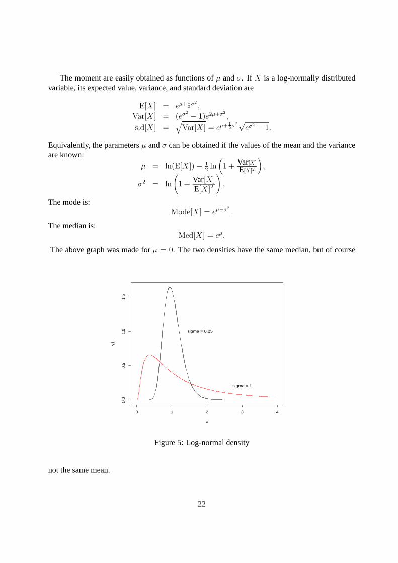
The above graph was made forµ = 0. The two densities have the same median, but of course

0 1 2 3 4

0.0

0.5

1.0

1.5

x

y1

sigma = 0.25

sigma = 1

Figure 5: Log-normal density

not the same mean.

22

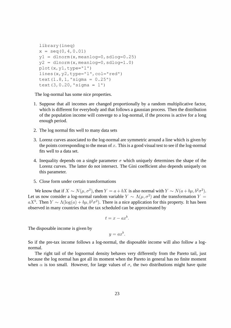
library(ineq)x = seq(0,4,0.01)y1 = dlnorm(x,meanlog=0,sdlog=0.25)y2 = dlnorm(x,meanlog=0,sdlog=1.0)plot(x,y1,type="l")lines(x,y2,type="l",col="red")text(1.8,1,"sigma = 0.25")text(3,0.20,"sigma = 1")

The log-normal has some nice properties.

1. Suppose that all incomes are changed proportionally by a random multiplicative factor,which is different for everybody and that follows a gaussianprocess. Then the distributionof the population income will converge to a log-normal, if the process is active for a longenough period.

2. The log normal fits well to many data sets

3. Lorenz curves associated to the log-normal are symmetricaround a line which is given bythe points corresponding to the mean ofx. This is a good visual test to see if the log-normalfits well to a data set.

4. Inequality depends on a single parameterσ which uniquely determines the shape of theLorenz curves. The latter do not intersect. The Gini coefficient also depends uniquely onthis parameter.

5. Close form under certain transformations

We know that ifX ∼ N(µ, σ2), thenY = a+ bX is also normal withY ∼ N(a+ bµ, b2σ2).Let us now consider a log-normal random variableY ∼ Λ(µ, σ2) and the transformationY =aXb. ThenY ∼ Λ(log(a) + bµ, b2σ2). There is a nice application for this property. It has beenobserved in many countries that the tax scheduled can be approximated by

t = x− axb.

The disposable income is given byy = axb.

So if the pre-tax income follows a log-normal, the disposable income will also follow a log-normal.

The right tail of the lognormal density behaves very differently from the Pareto tail, justbecause the log normal has got all its moment when the Pareto in general has no finite momentwhenα is too small. However, for large values ofσ, the two distributions might have quite

23

similar tails. This can be seen on a log-log graph. Let us takethe log of the density

log f(x) = − log x− log√2πσ − (log x− µ)2

2σ2

= − log2 x2σ2 + ( µ

σ2 − 1) log x− log√2πσ − µ2

2σ2

' (µσ2 − 1) log x− log

√2πσ − µ2

2σ2 for largeσ

The left tail of the log density behaves like a straight line for a large range ofx whenσ is largeenough.

0.0 0.2 0.4 0.6 0.8 1.0

0.0

0.2

0.4

0.6

0.8

1.0

p

Lc.lo

gnor

m(p

, par

amet

er =

0.2

5)

45° line

0.25

0.50

1.00

1.50

Figure 6: Log-normal Lorenz curves

library(ineq)p = seq(0,1,0.01)plot(p,Lc.lognorm(p, parameter=0.25),type="l",col="b rown")lines(p,Lc.lognorm(p, parameter=0.5),col="red")lines(p,Lc.lognorm(p, parameter=1.0),col="blue")lines(p,Lc.lognorm(p, parameter=1.5),col="green")lines(p,p)text(0.42,0.5,"45 ◦ line")text(0.8,0.68,"0.25")

24

text(0.8,0.58,"0.50")text(0.8,0.40,"1.00")text(0.8,0.20,"1.50")

We can give some more details on this distribution, concerning Gini coefficient and the Lorenzcurve. Let us callΦ(x) the standard normal distribution withΦ(x) = Prob(X < x). FromCowell (1995), we have Table 5. The Pietra index was found in Moothathua (1989).

Table 5: Various coefficients for the Log-Normal distribution

Coefficient of variation√

exp(σ2)− 1

Lorenz curve Φ(Φ−1(p)− σ)Pietra index 2Φ(σ2/2)− 1

Gini index 2Φ(σ/√2)− 1

Atkinson 1− exp(−1/2εσ2)

Generalized entropy exp((θ2 − θ)σ2/2)− 1θ2 − θ

The lognormal has an interesting poverty for poverty analysis. The mean is given byexp(µ+σ2/2) while the mode isexp(µ). A usual practice for defining a poverty line is the take eitherz1 = 0.5× the mean orz2 = 0.6× the mode. Using the properties of the lognormal, we can showthat these choices are not equivalent and can give rather different results. The two poverty linesare the same whenσ2 = 2 × log(0.6/0.5) = 0.37, which corresponds to a Gini index of 0.33.So, if we adopt a lognormal distribution for the French income, thenz1 < z2 because the Giniindex is lower than 0.30 while for China, we shall have just the contrary because the Gini indexis greater than 0.50.

Lognormal distributions are usually generated by multiplicative models. The first explanationof this type was proposed by Gibrat (1930). We start with an initial value for incomeX0. In thenext period, this income can grow or diminish according to a multiplicative and positive randomvariableFt

Xt = FtXt−1.

Taking the logs and using a recurrence, we have

logXt = log(X0) +∑

k

log(Fk).

By the central limit theorem, we get a log normal distribution. Note that the mechanism de-signed by Champernowne (1953) was very similar. We got a Pareto distribution only because aminimum value was imposed.

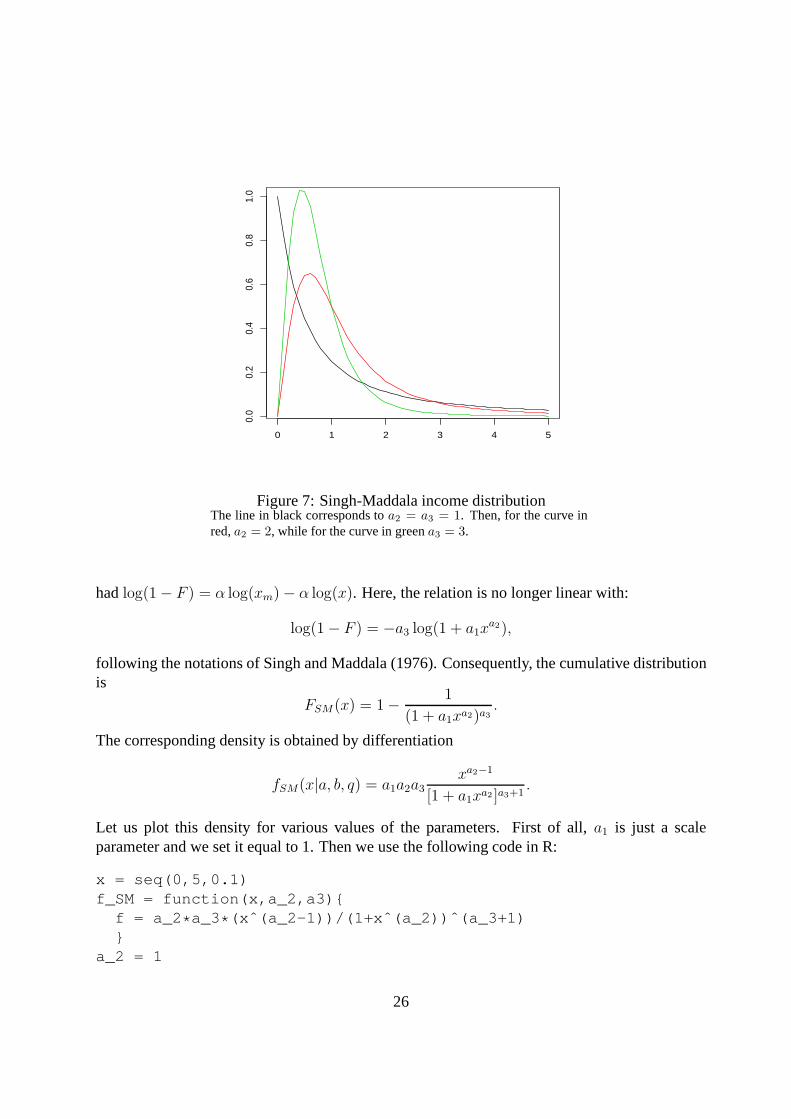
7.3 Singh-Maddala distribution∗

Singh and Maddala (1976) propose a justification of the old Burr XII distribution by consideringthe log survival function as a richer function ofx than what the Pareto does. With the Pareto we

25

0 1 2 3 4 5

0.0

0.2

0.4

0.6

0.8

1.0

Figure 7: Singh-Maddala income distributionThe line in black corresponds toa2 = a3 = 1. Then, for the curve inred,a2 = 2, while for the curve in greena3 = 3.

hadlog(1− F ) = α log(xm)− α log(x). Here, the relation is no longer linear with:

log(1− F ) = −a3 log(1 + a1xa2),

following the notations of Singh and Maddala (1976). Consequently, the cumulative distributionis

FSM(x) = 1− 1

(1 + a1xa2)a3.

The corresponding density is obtained by differentiation

fSM(x|a, b, q) = a1a2a3xa2−1

[1 + a1xa2 ]a3+1.

Let us plot this density for various values of the parameters. First of all, a1 is just a scaleparameter and we set it equal to 1. Then we use the following code in R:

x = seq(0,5,0.1)f_SM = function(x,a_2,a3){

f = a_2 * a_3* (xˆ(a_2-1))/(1+xˆ(a_2))ˆ(a_3+1)}

a_2 = 1

26

a_3 = 1plot(x,f_SM(x,a_2,a3),type="l",ylab="",xlab="")a_2=2lines(x,f_SM(x,a_2,a3),col=2)a_3 = 2lines(x,f_SM(x,a_2,a3),col=3)

The parameter of the Pareto distribution could easily be estimated using a linear regressionof log(1 − F ) over log(x) whereF is the natural estimator of the cumulative distribution. Herea non linear regression can be applied which minimized:

∑

[log(1− F (x)) + a3 log(1 + a1xa2)]2.

The uncentered moments of orderh and the Gini coefficient are expressed in term of theGamma function and can be found in McDonald and Ranson (1979)and McDonald (1984):

E(Xh) = bhΓ(1 + h/a2)Γ(a3 − h/a2)

Γ(a3)

with b = (1/a1)1/a2 as well as the Gini index:

G = 1− Γ(a3)Γ(2a3 − 1/a2)

Γ(a3 − 1/a2)Γ(2a3).

All the moment do not exist in this distribution. For a momentof orderh, we must have

a3 >h

a2.

If a3 > 1/a2, we can derive the Lorenz curve as

LC(p) = 1µ

∫ p

0b[(1− y)−1/a3 − 1]1/a2dy

= a3µ

∫ z

0t1/a2(1− t)a3−1/a2−1dt

= Iz(1 + 1/a2, a3 − 1/a2)

wherez = 1− (1− a3)1/a3 andIz(a, b) denotes the incomplete beta function ratio defined by:

IBz(a, b) =

∫ z

0ta−1(1− t)b−1dt

∫ 1

0ta−1(1− t)b−1dt

.

The Singh-Maddala distribution admit two limiting distributions, depending on the value ofa3. For a3 = 1, we have the Fisk (1961) distribution. Fora3 → ∞, we have the Weibulldistribution, to be detailed later on. So, depending on the value ofa3, the associated Lorenzcurves are supposed to cover a wide range of shapes. In the left panel, we kepta2 = 2 and leta3vary between 0.7 and 2. In the right panel, we kepta3 = 0.7 and leta2 vary between 2 and 3.5.The two black curves are identical. In one case the modification is more in the right part and inthe other case more in the left part. However, we note that theflexibility is not very strong.

The corresponding code using R is:

27

a2 = 2

0.0 0.2 0.4 0.6 0.8 1.0

0.0

0.2

0.4

0.6

0.8

1.0

p

LC

sin

gh

(p,

a,

0.7

)

a3=0.7

a3=0.9

a3=2

a3 = 0.7

0.0 0.2 0.4 0.6 0.8 1.0

0.0

0.2

0.4

0.6

0.8

1.0

p

LC

sin

gh

(p,

a,

0.7

)

a2=2.0

a2=2.5

a2=3.5

Figure 8: Singh-Maddala Lorenz curves when varyinga2 or a3

LCsingh <- function(p,a,q){pbeta((1 - (1 - p)ˆ(1/q)), (1 + 1/a), (q-1/a))}p = seq(0,1,0.01)a = 2plot(p,LCsingh(p, a,0.7),type="l")lines(p,LCsingh(p, a,0.9),type="l",col="red")lines(p,LCsingh(p, a,2),type="l",col="blue")lines(p,p)text(0.8,0.24,"a3=0.7")text(0.8,0.34,"a3=0.9",col="red")text(0.8,0.48,"a3=2",col="blue")

7.4 Weibull distribution ∗

The Weibull distribution is a nice two parameter distribution where all moments exists. It isobtained as a special case of the three parameter Singh Maddala distribution, fora3 → ∞. Thisrelation explains that the cumulative distribution has an analytical form:

F (x) = 1− exp(−(kx)α).

By differentiation, we get the density

f(x) = k α (k x)α−1 exp−(k x)α.

28

0 1 2 3 4

0.0

0.2

0.4

0.6

0.8

1.0

1.2

x

alpha=0.5

alpha=1.2

alpha=2.0

Figure 9: Weibull income distribution

We have a plot of this density in Figure 9. Forα < 1, the density has the shape of the Paretodensity, which means that it has no finite maximum. Forα = 1, it cuts they axis. Asα grows,there is less and less inequality and the function concentrates around its mean. Plausible valuesfor α corresponding to usual income distributions are[1.5− 2.5].

Theh− th moments around zero are given by

µh =Γ(1 + h/α)

kh

whereΓ(a) is the gamma function defined by

Γ(a) =∫ ∞

0ua exp(−u) du

The coefficient of variation (the ratio between the standarddeviation and the mean) is equal to:

CV =

√

Γ((α + 2)/α)− Γ(α+ 1)/α)2

Γ((α + 1)/α)

As we have the direct expression of the distribution, the Gini coefficient and the Lorenz curvesare directly available. We find the expression of the Lorenz curve and the Gini index for instancein Krause (2014):

LC = 1− Γ(− log(1− p), 1 + 1/α)

Γ(1 + 1/α),

29

whereΓ(x, α) is the incomplete Gamma function.We regroup in Table 6 some of these results. We did not manage to fully complete this Table,

presumably because the Weibull distribution is not very often used for modelling the incomedistribution.

Table 6: Several indices for the Weibull distribution

Coefficient of variation

√

Γ((α+ 2)/α)− Γ(α + 1)/α)2

Γ((α+ 1)/α)

Lorenz curve 1− Γ(− log(1− p), 1 + 1/α)Γ(1 + 1/α)

Pietra indexGini index 1− 2−1/α

AtkinsonGeneralized entropy

Note that there are various ways of writing the density of theWeibull, concerning the scaleparameterk. Either(kx)α or (x/k)α. For inference, it might even be convenient to considerkxα.So be careful. InR, the density is available asdweibull(x, shape, scale = 1) usingthe parameterizations(x/k)α.

The Weibull distribution shares with the Pareto, the Sing-Maddala distribution a commonfeature which is to have an analytical cumulative distribution. If we rearrange its expression andtake logs, we get:

log(− log(1− F )) = α log(kx).

So that it is easy to check if a sample has a Weibull distribution. And by the way gives a methodto estimate the parameterα.

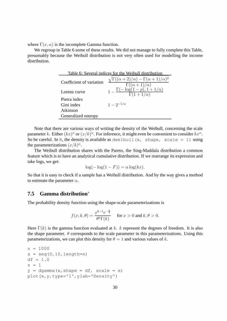
7.5 Gamma distribution∗

The probability density function using the shape-scale parameterizations is

f(x; k, θ) =xk−1e−

x

θ

θkΓ(k)for x > 0 andk, θ > 0.

HereΓ(k) is the gamma function evaluated atk. k represent the degrees of freedom. It is alsothe shape parameter.θ corresponds to the scale parameter in this parameterizations. Using thisparameterizations, we can plot this density forθ = 1 and various values ofk.

n = 1000x = seq(0,10,length=n)df = 1.0s = 1y = dgamma(x,shape = df, scale = s)plot(x,y,type="l",ylab="Density")

30

0 2 4 6 8 10

0.0

0.2

0.4

0.6

0.8

1.0

x

Den

sity

DF = 1

DF = 2

DF = 3

DF = 4

DF = 5

Figure 10: Gamma density

text(8,1.0-df/15,paste("DF = ",toString(df)),col=df)for (df in c(2,3,4,5)){

y = dgamma(x,shape = df, scale = s)lines(x,y,col = df)text(8,1.0-df/15,paste("DF = ",toString(df)),col=df)}

The cumulative distribution function is the regularized gamma function:

F (x; k, θ) =∫ x

0f(u; k, θ) du =

γ(

k, xθ

)

Γ(k)

whereγ(k, x/θ) is the lower incomplete gamma function.The skewness is equal to2/

√k, it depends only on the shape parameterk and approaches

a normal distribution whenk is large (approximately whenk > 10). The mean iskθ and thevariancekθ2.

Rather easy to estimate. Bayesian inference. InR, dgamma, pgamma, qgamma, rgammausing the same parametrization.

7.6 Variations around the Pareto distribution∗

We have presented the Pareto I distribution. Pareto distribution have a right tail which is a powerfunction. Several variants were proposed in the literature, a good account of which is given in

31

2 4 6 8 10

0.0

0.2

0.4

0.6

0.8

1.0

x

P1

Pareto IPareto IIPareto IIIPareto IV

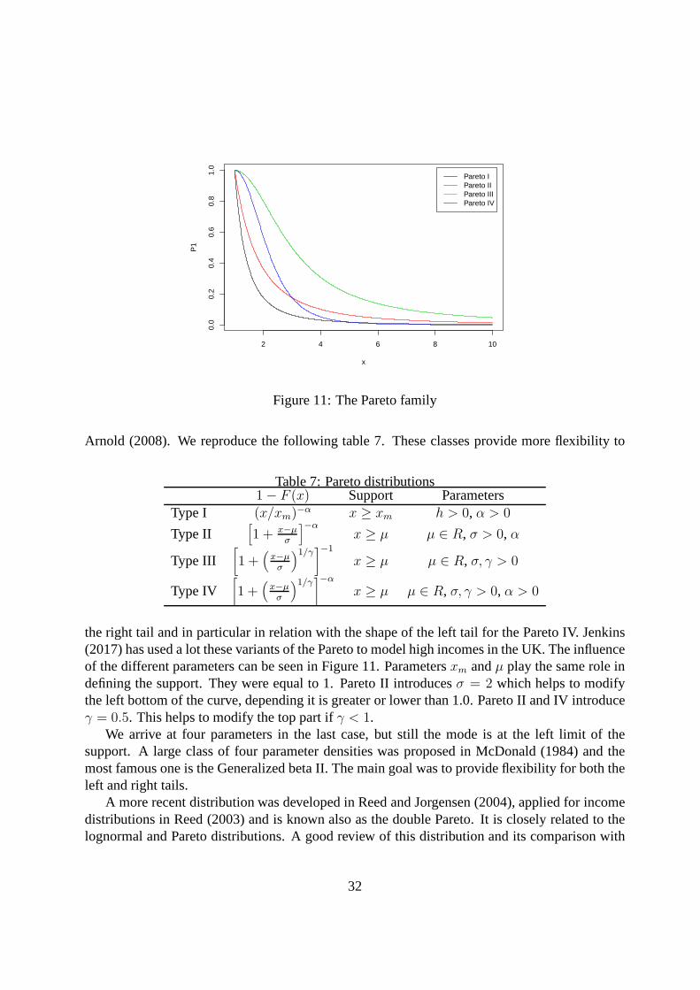
Figure 11: The Pareto family

Arnold (2008). We reproduce the following table 7. These classes provide more flexibility to

Table 7: Pareto distributions1− F (x) Support Parameters

Type I (x/xm)−α x ≥ xm h > 0, α > 0

Type II[

1 + x−µσ

]−αx ≥ µ µ ∈ R, σ > 0, α

Type III[

1 +(

x−µσ

)1/γ]−1

x ≥ µ µ ∈ R, σ, γ > 0

Type IV[

1 +(

x−µσ

)1/γ]−α

x ≥ µ µ ∈ R, σ, γ > 0, α > 0

the right tail and in particular in relation with the shape ofthe left tail for the Pareto IV. Jenkins(2017) has used a lot these variants of the Pareto to model high incomes in the UK. The influenceof the different parameters can be seen in Figure 11. Parametersxm andµ play the same role indefining the support. They were equal to 1. Pareto II introducesσ = 2 which helps to modifythe left bottom of the curve, depending it is greater or lowerthan 1.0. Pareto II and IV introduceγ = 0.5. This helps to modify the top part ifγ < 1.

We arrive at four parameters in the last case, but still the mode is at the left limit of thesupport. A large class of four parameter densities was proposed in McDonald (1984) and themost famous one is the Generalized beta II. The main goal was to provide flexibility for both theleft and right tails.

A more recent distribution was developed in Reed and Jorgensen (2004), applied for incomedistributions in Reed (2003) and is known also as the double Pareto. It is closely related to thelognormal and Pareto distributions. A good review of this distribution and its comparison with

32

the Pareto and the lognormal distributions is given in Mitzenmacher (2004). Both the General-ized Beta II and the Double Pareto have four parameters, but are uni-modal.

7.7 Which density should we select?∗

In his book, Cowell (1995) is not very optimistic about the more complicated four parameterdensities. Their parameters are hard to interpret and they are difficult to estimate. He is more infavour of the Pareto density, which is fact has a single important parameter (xm defines only thesupport of the density), the two parameter lognormal and eventually the gamma density. He doesnot like the more complicated densities like the Singh-Maddala and even more the generalizedBeta II. In Lubrano and Protopopescu (2004), we make use of the two parameter Weibull densityto estimate generalized Lorenz curves and rank bibliometric distributions. The three parametersSingh-Maddala distribution is quite simple to estimate as the authors propose a method based ona regression. The three parameter generalized gamma density has a very awkward parameteri-zation so that it has the reputation of being not estimable bymaximum likelihood on individualdata.

The Pareto density and its variants are nice for modelling high incomes, see in particularJenkins (2017). The gamma density is nice for modelling mid range incomes as well as thelog-normal density. Cowell (1995) thus prefers two parameter densities for modelling particu-lar portions of the income distribution. We can conclude that using mixture of two parameterdensities might be the best alternative for modelling the complete income distribution.

8 Pigou-Dalton transfers and Lorenz ordering

Pigou-Dalton transfers are mean-preserving equalizing transfers of income. They involve amarginal transfer of 1 from a richer person belonging to percentile pr to a poorer person be-longing to percentilepp < pr) that keeps total income constant. These equalizing transfers havethe consequence of moving the Lorenz curve unambiguously closer to the line of perfect equal-ity. This is because such transfers do not affect the value ofL(p) for all p up topp and for allpgreater thanpr, but they increaseL(p) for all p betweenpp andpr.

8.1 Lorenz ordering

Let us consider two income distributionsA andB, where distributionB is obtained by applyingPigou-Dalton transfers toA. Hence, the Lorenz curveLB(p) of distributionB will be everywhereabove the Lorenz curveLA(p) of distributionA. Inequality indices which obey the principle oftransfers will unambiguously indicate more inequality inA than inB. We will also say that if

LB(p)− LA(p) ≥ 0 ∀p

thenB Lorenz dominatesA.

33

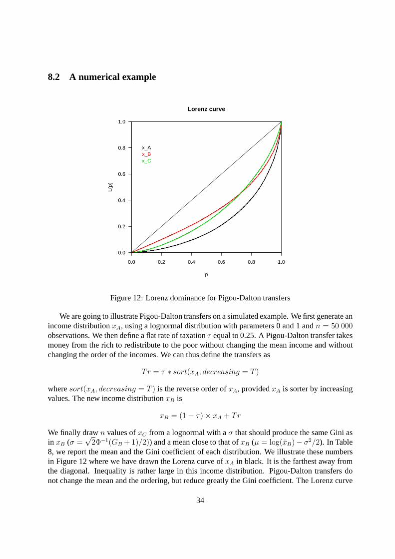
8.2 A numerical example

0.0 0.2 0.4 0.6 0.8 1.0

0.0

0.2

0.4

0.6

0.8

1.0

Lorenz curve

p

L(p)

x_Ax_Bx_C

Figure 12: Lorenz dominance for Pigou-Dalton transfers

We are going to illustrate Pigou-Dalton transfers on a simulated example. We first generate anincome distributionxA, using a lognormal distribution with parameters 0 and 1 andn = 50 000observations. We then define a flat rate of taxationτ equal to 0.25. A Pigou-Dalton transfer takesmoney from the rich to redistribute to the poor without changing the mean income and withoutchanging the order of the incomes. We can thus define the transfers as

Tr = τ ∗ sort(xA, decreasing = T )

wheresort(xA, decreasing = T ) is the reverse order ofxA, providedxA is sorter by increasingvalues. The new income distributionxB is

xB = (1− τ)× xA + Tr

We finally drawn values ofxC from a lognormal with aσ that should produce the same Gini asin xB (σ =

√2Φ−1(GB + 1)/2)) and a mean close to that ofxB (µ = log(xB)− σ2/2). In Table

8, we report the mean and the Gini coefficient of each distribution. We illustrate these numbersin Figure 12 where we have drawn the Lorenz curve ofxA in black. It is the farthest away fromthe diagonal. Inequality is rather large in this income distribution. Pigou-Dalton transfers donot change the mean and the ordering, but reduce greatly the Gini coefficient. The Lorenz curve

34

Table 8: The effects ofPigou-Dalton transfers

Distribution Mean GiniBefore redistributionxA 1.647 0.521After redistributionxB 1.647 0.331Log normalxC 1.648 0.331

corresponding toxB is in red. It does not intersectLA even if the distribution ofxB cannot be alognormal.

The last samplexC should have a Gini coefficient close to that ofxB. However, its Lorenzcurve crosses that ofxB because it is obtained in a totally different way, implying differenttransfers which are not Pigou-Dalton.

TheRcode is as follows:

n = 50000x_A = sort(rlnorm(n,0,1))tau = 0.25Tr = tau * sort(x_A,decreasing = T)x_B = (1-tau) * x_A + Tr

s = sqrt(2) * qnorm((gini(x_B)+1)/2)mu = log(mean(x_A))-0.5 * sˆ2x_C = rlnorm(n,mu,s)

cat(mean(x_A),gini(x_A),"\n")cat(mean(x_B),gini(x_B),"\n")cat(mean(x_C),gini(x_C),"\n")

plot(Lc(x_A))lines(Lc(x_B),col=2)lines(Lc(x_C),col=3)

8.3 Generalized Lorenz Curve

The generalized Lorenz curve (GLC) introduced by Shorrocks(1983) is the most importantvariation of the Lorenz curve (LC). The LC is scale invariantand is thus only an indicator ofrelative inequality. However, it does not provide a complete basis for making social welfarecomparisons. The Shorrocks proposal is the generalized Lorenz curve defined as:

GLC(p) = µLC(p) =∫ p

0F−1(y)dy

35

Note thatGLC(0) = 0 andGLC(1) = µ. A distribution with a dominating GLC providesgreater welfare according to all concave increasing socialwelfare functions defined on individualincomes (Kakwani 1984, and the surveys of Davies et al. 1998 and Sarabia 2008). On the otherhand, the GLC is no longer scale-free and in consequence it determines any distribution withfinite mean.

The usual Lorenz curve when one focusses his attention on inequality only. The GeneralizedLorenz curves mixes concerns for inequality and for the mean, so it is related to welfare compar-isons. The order induced by GLC is in fact the second-order stochastic dominance that we shalleventually study in a next chapter. This order is a new partial ordering, and sometimes it allowsa bigger percentage of curves to be ordered than in the Lorenzordering case.

8.4 Lorenz Ordering for usual distributions∗

Lorenz curves can be used to define an ordering in the space of the of distributions. If twodistribution functions have associated Lorenz curves which do not intersect, they can be orderedwithout ambiguity in terms of welfare functions which are symmetric, increasing and quasi-concave (see Atkinson 1970. We express this formally with the definition:

Definition 2 LetA andB be two income distributions. DistributionB is preferred to distributionA in the Lorenz sense iff:

B �L A ⇔ LB(p) ≥ LA(p), ∀p ∈ [0, 1].

If B �L A, thenB exhibits less inequality thanA in the Lorenz sense. Note that the Lorenzorder is a partial order and is invariant with respect to scale transformation.

It is fairly possible now to characterize Lorenz dominance by restrictions over the parameterspace if the two random variables have the same class of distributions. For some parametricfamilies the restrictions will be very simple, and by the waywill imply rather simple parametricstatistical tests. We have derived Lorenz curves for the most important parametric densities,leaving aside those which were too complex and which are surveyed in Sarabia (2008).

We present first results for the Pareto and the log-normal.

• Pareto: LetXi ∼ P (αi, xmi). Then

FX1�L FX2

⇔ α1 ≥ α2

• Log-Normal: LetXi ∼ LN(µi, σ2i ). Then

FX1�L FX2

⇔ σ1 ≤ σ2

The proof of these results is straightforward because in thetwo cases, the Lorenz curves neverintersect as they depend on a single parameter.

The case of the Singh-Maddala distribution is more difficultto establish. Its Lorenz curvedepends on two parameters and may thus intersect. Let us notethe normalized distribution asF = 1− 1/(1 + xa)q. Then from Sarabia (2008) we get:

36

Theorem 3 LetXi ∼ SM(ai, qi), i = 1, 2 be two Singh-Maddala distributions. Then

X1 �L X2 ⇔ a1q1 ≤ a2q2, anda1 ≤ a2.

The proof of this result is more delicate to establish and thestatistical test of these restrictions isslightly more difficult to implement.

9 Parametric Lorenz curves∗

We first recall in a table the expression of the Lorenz curve for some standard income distribution.We gave a theorem characterizing a Lorenz curve. This means that any function following these

Table 9: Lorenz and Gini indices for classical income distributionsDistribution Lorenz curve Gini indexPareto I L(p) = 1− (1− p)1−1/α 1

2α−1

Lognormal L(p) = Φ(Φ−1(p)− σ) 2Φ(σ/√2)− 1

Weibull L(p) = 1− Γ(− log(1− p), 1 + 1/α)Γ(1 + 1/α)

1− 2−1/α

Singh-Maddla L(p) = Iz(q + 1/a, q − 1/a) 1− Γ(q)Γ(2q−1/a)Γ(q−1/a)Γ(2q)

properties is a Lorenz curve. So we can try to investigate this class of functions. We followSarabia (2008), but not all the details. The first parametricform which was given in the literatureis

L(p) = pα exp(−β(1− p)),

with α ≥ 1 andβ > 0.A family of Lorenz curves which is interesting and easy to understand is build around the

Pareto family. We can generalize the Lorenz curve of the Pareto by adding one more parameter,so as to get:

L(p) = [1− (1− p)1−1/α]β.

If β = 1, we have the asymmetric Lorenz curve of the Pareto. Ifβ = 1/(1− 1/α), we obtain asymmetric Lorenz curve, thus having a similar property to that of the Lognormal. The underlyingdensity to this Lorenz curve combines properties of the Pareto and of the Lognormal. Moregeneral expressions are given in Sarabia (2008).

Let us explore these functional forms using R.

LCgen <- function(p,alpha,beta){smlc <- (1-(1-p)ˆ(1-1/alpha))ˆbetasmlc}

p = seq(0,1,0.01)plot(p,LCgen(p, 1.5,1),type="l")text(0.93,0.45,"1.5, 1.0")lines(p,LCgen(p,3,1.5),type="l",col="red")

37

text(0.7,0.50,"3.0, 1.5")lines(p,LCgen(p,4,2),type="l",col="blue")text(0.5,0.10,"4.0, 2.0")lines(p,p)text(0.42,0.5,"45 ◦ line")

0.0 0.2 0.4 0.6 0.8 1.0

0.0

0.2

0.4

0.6

0.8

1.0

p

LCge

n(p,

1.5

, 1)

1.5, 1.03.0, 1.5

4.0, 2.0

45° line

Figure 13: The flexibility of a two parameter Lorenz curve

It is remarkable that play playing with two parameters, we can obtain very different shapes andin particular many points of intersection in a much simpler way than with the Singh-Maddaladistribution. The Gini coefficient has a simple expression and is equal to

G = 1− 2

1− 1/αB(1/(1− 1/α), β + 1)

38

where B(.,.) is the incomplete Beta function.It would be nice to compute the Atkinson and GE indices using the formula given above

using the Lorenz curve. Derive the corresponding densities.

39

10 Exercises

10.1 Empirics

Using the previous FES data set, the softwareR and the packageineq , compare the empiricalLorenz curve to those obtained for the Pareto and Log-normal. Say which distribution would fitthe best. Redo the same exercise limiting the data to high incomes.

10.2 Gini coefficient

We have seen that the Gini coefficient could be seen as the covariance between a variable and itsrank, namely:

G =2

µCov(y, F (y)).

As Cov(y, F (y)) =∫

y(F (y)− 1/2)dF (y), use integration by parts to show that

Cov(y, F (y)) =1

2

∫

F (x)[1− F (x)]dx,

and give the corresponding form of the Gini. Give the value ofF for which the Gini is maximum.What can you deduce of this result as a property of the Gini index?

10.3 LogNormal

Compute the value of the Generalized Entropy index forθ = 0 andθ = 1. Comment your result.Does it hold in the general case of a general distribution. Dothe same calculation for the Paretodensity.

10.4 Uniform

The uniform density between 0 andxm is sometimes used in theoretical economic paper todescribe the income distribution. It writes:

f(x) =1

xm1I(x ≤ xm)

This density has strange properties that we shall now explore.

1. Compute the mean and the variance

2. Calculate the expression of the cumulative distribution

3. Using the inverse of this cumulative distribution compute the expression of the Lorenzcurve

L(p) =1

µ

∫ p

0F−1(t)dt

40

4. CompareL(p) with that of the Pareto distribution

5. Compute the Gini index corresponding to the uniform distribution using

G = 1− 2∫ 1

0L(p)dp

6. Verify that you obtain the same result using

G = 1− 1

µ

∫ xm

0[1− F (t)]2dt

10.5 Singh-Maddala∗

Find an example where two Lorenz curves associated to the Singh-Maddala distribution intersect.Use the graphs produced byR for this. Mind that the parametrization adopted inR for thefunction Lc.singh is awkward. Use the function provided in the text.

10.6 Logistic∗

The logistic density is very close to the normal density, butit has nicer properties, such as inparticular an analytical cumulative distribution. We have

f(x) =e−(x−µ)/s

s(1 + e−(x−µ)/s)2

F (x) =1

1 + e−(x−µ)/s

with meanµ and varianceπ2s2/3. Find the log logistic distribution using the adequate transfor-mation. Find the Gini coefficient. This is the Fisk distribution.

10.7 Weibull∗

Show that whena3 → ∞ in the Singh-Maddala distribution, we get the Weibull.

References

Arnold, B. C. (2008). Pareto and generalized Pareto distributions. In Chotikapanich, D., editor,Modeling Income Distribuions and Lorenz Curves, volume 5 ofEconomic Studies in Equality,Social Exclusion and Well-Being, chapter 7, pages 119–145. Springer, New-York.

Atkinson, A. (1970). The measurement of inequality.Journal of Economic Theory, 2:244–263.

Champernowne, D. (1953). A model of income distribution.Economic Journal, 63:318–351.

41

Cowell, F. (1995).Measuring Inequality. LSE Handbooks on Economics Series. Prentice Hall,London.

Davidson, R. (2009). Reliable inference for the gini index.Journal of Econometrics, 150:30–40.

Davies, J. B., Green, D. A., and Paarsch, H. J. (1998). Economic statistics and social welfarecomparisons: A review. In Ullah, A. and Giles, D. E. A., editors,Handbook of Applied Eco-nomic Statistics, volume 155 ofStatistics: Textbooks and Monographs, pages 1–38. Dekker,New York, Basel and Hong-Kong.

Deaton, A. (1997).The Analysis of Household Surveys. The John Hopkins University Press,Baltimore and London.

Donaldson, D. and Weymark, J. (1980). A single-parameter generalization of the gini indices ofinequality.Journal of Economic Theory, 22(1):67–86.

Duclos, J.-Y. and Araar, A. (2006).Poverty and Equity: Measurement, Policy and Estimationwith DAD. Springer, Newy-York.

Fisk, P. (1961). The graduation of income distributions.Econometrica, 29:171–185.

Gastwirth, J. L. (1971). A general definition of the lorenz curve. Econometrica, 39(6):1037–1039.

Gibrat, R. (1930). Une loi des reparations economiques: l’effet proportionnel. Bulletin deStatistique General, France, 19:469.

Giles, D. E. A. (2004). Calculating a standard error for the gini coefficient: Some further results.Oxford Bulletin of Economics and Statistics, 66(3):425–433.

Jenkins, S. P. (2017). Pareto models, top incomes and recenttrends in uk income inequality.Economica, 84(334):261–289.

Kakwani, N. (1984). Welfare ranking of income distributions. In Basmann, R. and Rhodes, G.,editors,Advances in Econometrics, volume 3, pages 191–213. JAI Press.

Krause, M. (2014). Parametric Lorenz curves and the modality of the income density function.Review of Income and Wealth, 60(4):905–929.

Lubrano, M. and Protopopescu, C. (2004). Density inferencefor ranking european researchsystems in the field of economics.Journal of Econometrics, 123(2):345–369.

McDonald, J. (1984). Some generalised functions for the size distribution of income.Economet-rica, 52(3):647–663.

McDonald, J. B. and Ranson, M. R. (1979). Functional forms, estimation techniques and thedistribution of income.Econometrica, 47(6):1513–1525.

42

Mitzenmacher, M. (2004). A brief history of generative models for power law and lognormaldistributions.Internet Mathematics, 1(2):226–251.

Moothathua, T. S. K. (1989). On unbiased estimation of Gini index and Yntema-Pietra indexof lognormal distribution and their variances.Communications in Statistics - Theory andMethods, 18: 2,(2):661–672.

Piketty, T. (2000).Les hauts revenus en France au 20ieme siecle: Inegalites et redistributions,1901-1998. Grasset, Paris.

Piketty, T., Yang, L., and Zucman, G. (2017). Capital accumulation, private property and risinginequality in China, 1978-2015. Technical Report Working Paper 23368, NBER.

Reed, W. J. (2003). The Pareto law of incomes: an explanationand an extension.Physica, A319:469–486.

Reed, W. J. and Jorgensen, M. (2004). The double pareto-lognormal distribution: A new para-metric model for size distributions.Communications in Statistics - Theory and Methods,33(8):1733–1753.

Sarabia, J. M. (2008). Parametric lorenz curves: Models andapplications. In Chotikapanich, D.,editor,Modeling Income Distribuions and Lorenz Curves, volume 5 ofEconomic Studies inEquality, Social Exclusion and Well-Being, chapter 9, pages 167–190. Springer, New-York.

Sen, A. (1976). Poverty: an ordinal approach to measurement. Econometrica, 44(2):219–231.

Sen, A. K. (1973).On Economic Inequality. Clarendon Press, Oxford.

Shorrocks, A. F. (1983). Ranking income distributions.Economica, 50(197):3–17.

Singh, S. and Maddala, G. (1976). A function for the size distribution of incomes.Econometrica,44:963–970.

Xu, K. (2003). How has the literature on gini’s index evolvedin the past 80 years? Economicsworking paper, Dalhousie University. Available at SSRN: http://ssrn.com/abstract=423200 ordoi:10.2139/ssrn.423200.

Yitzhaki, S. (1998). More than a dozen alternative ways of spelling Gini. Research in EconomicInequality, 8:13–30.

43