Embed Size (px)
Citation preview

RETRENCHMENT AND RENEWAL:
THE ECONOMIC AND DEMOGRAPHIC OUTLOOK
FOR SOUTHEAST MICHIGAN THROUGH 2040
Prepared by
Donald R. Grimes George A. Fulton
Institute for Research on Labor, Employment, and the Economy
Prepared for
Southeast Michigan Council of Governments
March 2012
Preparation of this document may be financed in part through grants from and in cooperation with the Michigan Department of Transportation with the assistance of the U.S. Department of Transportation’s Federal Highway Administration and Federal Transit Administration; the Michigan Department of Natural Resources with the assistance of the U.S. Environmental Protection Agency; the Michigan State Police Office of Highway Safety Planning; and local membership contributions. This document was prepared in March 2012 for the Southeast Michigan Council of Governments.


Retrenchment and Renewal: The Economic and Demographic Outlook for Southeast Michigan
Through 2040
By DONALD R. GRIMES, senior research specialist, and GEORGE A. FULTON, research professor, Institute for Research on Labor, Employment, and the Economy , University of Michigan
Abstract
The Southeast Michigan economy is now emerging from its most catastrophic period in our lifetime—during the first decade of the 2000s, the region lost virtually all of the jobs it had garnered during the robust 1990s. There is evidence that the regional economy has now made a good start in returning to positive job growth, and our view is that its competitive position has turned around and job growth will be sustained. According to our economic and demographic outlook for Southeast Michigan through 2040, growth will be much more subdued than what we saw prior to the extended downturn, and considerably less rosy than what we anticipated several years ago. We now expect that by 2040 employment in the region will still remain slightly below its peak level achieved in 2000. One consequence of the poor performance of the local economy from 2000 to 2009 is a permanent loss of population. Accelerating growth in the over-65 population and low in-migration rates for young adults will limit the region’s ability to expand, and these demographics will hang over the longer-term renewal of the economy. It’s hard to fathom in our current high unemployment environment, but the looming problem down the road will be labor shortages, particularly of workers with skills that mesh with the emerging knowledge- and information-based economy.

Acknowledgments
Many people kindly offered their time and expertise to us in putting this study together.
We are very grateful to the members of SEMCOG’s Forecast Technical Advisory
Committee for their ideas and critiques of the methodology and preliminary results. We
extend a special thanks to Xuan Liu of SEMCOG for his helpful leadership in
coordinating the project and interacting with the authors. We would like to give
particular recognition to Jacqueline Murray at IRLEE, University of Michigan, for
enhancing the quality of the presentation with her production and editorial skills. The
authors are solely responsible, though, for the interpretations and any errors of omission
or commission in this study.
ii

Table of Contents
List of Data Displays ......................................................................................................... iv
Introduction..........................................................................................................................1
Method .................................................................................................................................8
Schematic Outline of the Demographic and Economic Structure .......................................9
Inputs to the Forecast .........................................................................................................13
Inputs Related to the Demographics .............................................................................14 Inputs Related to the Economy .....................................................................................17
Forecast for Southeast Michigan through 2040.................................................................21
Demographics ...............................................................................................................22 Employment ..................................................................................................................26 Income...........................................................................................................................29
Alternative Forecast Scenarios ..........................................................................................31
Alternative Scenario 1: Regional Auto Industry Takes Another Big Hit .....................32 Alternative Scenario 2: Growing Like Pittsburgh........................................................35
Looming Labor Shortages..................................................................................................38
Conclusion .........................................................................................................................40
References..........................................................................................................................43
About the Authors..............................................................................................................44
iii

List of Data Displays
Table
1. Analysis of Private-Sector Employment Change, 2001 to 2010, Seven-County SEMCOG Region .........................................................................................................4
Figures
1. Distribution of U.S. Population by Age Categories, 1990, 2010, 2040 .....................15
2. Distribution of Population by Age Categories, U.S. vs. SEMCOG Region, 2010.....16
3. Distribution of U.S. Real GDP (Chained 2005$), 1990 –2040...................................17
4. Detroit Three Light Vehicle Sales, 1991–2011 ..........................................................20
5. Detroit Three Market Share of U.S. Light Vehicle Sales, 1991–2011 .......................20
6. Population of SEMCOG Region, 1990 –2040..............................................................22
7. Components of Population Change, SEMCOG Region, 1990 –2040 ........................23
8. Population Distribution by Age Categories, SEMCOG Region, 2010 and 2040.......25
9. Population Distribution by Age Categories, U.S. vs. SEMCOG Region, 2040 .........26
10. Total Employment in SEMCOG Region, 1990 –2040 ...............................................27
11. Change in Employment by Industry, SEMCOG Region, 2010 – 40...........................28
12. Average Annual Growth in Inflation-Adjusted Personal Income Per Capita, SEMCOG Region, 1990 –2040...................................................................................30
13. Alternative Forecast of Employment in Motor Vehicle and Parts Manufacturing, SEMCOG Region, 2001– 40.......................................................................................33
14. Alternative Forecasts of Total Employment (Auto scenario), SEMCOG Region, 2001– 40......................................................................................................................35
15. Alternative Forecasts of Total Employment (“Like Pittsburgh” scenario), SEMCOG Region, 2001– 40.......................................................................................36
16. Alternative Forecasts of Total Employment (Autos and “Like Pittsburgh”), SEMCOG Region, 2001– 40.......................................................................................37
iv

Introduction
First, the bad news. Over the past decade the Southeast Michigan region,1 and the
state of Michigan as a whole for that matter, have suffered through the worst economic
crisis in our lifetime. From 2000 to 2009, the Southeast Michigan region lost an
astounding 351,000 jobs,2 unfathomable at the beginning of the decade. Indeed, the
region gained almost 357,000 jobs in the robust growth era between 1990 and 2000, and
subsequently lost virtually all of them, in number, over the following nine years. Just shy
of 198,000 of the job losses—over half of them—occurred in a single year, during the
devastating crash of 2009. Some of those losses are likely permanent.
The hardship wrought over the past decade shows its face in many ways: An
unemployment rate that is far too high and only creeping down slowly. Too many
families are under water on their mortgages. Too many businesses remain reluctant to
hire. The greatest risk is a widespread relinquishing of hope for improvement—the loss
of optimism.
We view the past decade as a period of retrenchment consistent with the
dictionary definition of the word: a reduction, a cutting down, a paring away. This was
certainly the case with the activity still most integral to the economic fortunes of the
region, the domestic automotive industry. The Detroit Three (General Motors, Ford, and
Chrysler) were engaged in restructuring activities since the mid-2000s, and accelerated
1Throughout this report we use the same definition of Southeast Michigan as does the Southeast Michigan Council of Governments: Livingston, Macomb, Monroe, Oakland, St. Clair, Washtenaw, and Wayne counties. 2Throughout this report, the employment data are based on the measure published by the U.S. Bureau of Economic Analysis [6], and as such, include the self-employed, farm workers, and military personnel. The exception is the employment data reported in table 1, which are published by the U.S. Bureau of Labor Statistics [7].

2
those efforts later in the decade, spurred by looming bankruptcy proceedings which then
materialized for Chrysler and General Motors.
Now for the better news. There is light at the end of the tunnel, and in some
ways, we are emerging from the tunnel. The path taken by the auto industry shows that
retrenchment is not necessarily synonymous with collapse or the abandonment of hope.
From the bankruptcy proceedings, the auto companies have seen renewed growth, much
to the benefit of the region as a whole; all three of them are now making a profit, albeit
with a smaller work force. Retrenchment can also be the precursor to an era of renewal,
if we have the wherewithal and the motivation to get there. We remain optimistic that we
can and will do better.
This point of view is reflected in our forecast for the region. But this assessment
also has support from the data that have come in since the crash of 2009, particularly
from the most recent numbers. The national press has seized on these numbers in recent
months to trumpet Michigan’s comeback, seeing the state “starting to roll again,” “getting
back some lost swagger,” and observing that “These days, people think about Detroit
differently.” CNN, Bloomberg, and other national outlets have described Detroit as the
next Silicon Valley. And a few months ago, Bloomberg constructed a new index that
showed Michigan’s economy recovering at the second-fastest pace in the United States
(oil-rich North Dakota is first). We have a long way to go to be sure, but we’ve made a
good start and it is heartening that we are no longer viewed as the nation’s economic
caboose. Obviously, the region has assets that create opportunities within, and
recognition outside, its borders.

3
Exuberance should be tempered, however. We are extricating ourselves from a
very deep hole, and recovering from a recession induced by a financial crisis is a slow
climb. Although we see growth for the region in the years ahead, our growth forecast is
more muted now than we anticipated several years ago. The details are in the numbers,
which make up much of the rest of this report.
To better understand the recent path of the regional economy, the first set of
numbers we consider, in table 1, is the private-sector employment trends annually for the
region from 2001 to 2010. These data also isolate the manufacturing sector and its
automotive industry component.3 In addition to summarizing the employment path
annually in the first row of each entry, the table contains a breakout of those paths into
two subcomponents. The breakouts are unique to this study, and allow us to gain greater
insight into the employment outcomes reflected in the total changes for each year. The
first of the breakouts identifies the effect of national economic change on the respective
local employment outcome, and the second isolates the effect of local economic events
and policy, that is, the locally influenced change. An analogy to the national control
change would be the quality of the horse the region draws for a race, and for the locally
influenced change, the region’s skills as a jockey. Another analogy would be,
respectively, the cards the region draws in a game, and how it plays them.
Specifically, the national change component is a control scenario that shows what
would have happened if employment in the local industries had changed year to year at
exactly the same rate as the corresponding national industry, defined at the six-digit
3These data are from the U.S. Bureau of Labor Statistics, Quarterly Census of Employment and Wages [7], in addition to unpublished data estimated by the authors. The data reported here are a summation of both the published and estimated data at the six-digit NAICS code level, and may differ slightly from the published totals.
Table 1
Analysis of Private-Sector Employment Change, 2001 to 2010, Seven-County SEMCOG Region
2001 Employment 2001-02 2002-03 2003-04 2004-05 2005-06 2006-07 2007-08 2008-09 2001–09 2009-10
Total private Total change 1,978,872 –51,948 –37,370 –15,284 1,189 –40,609 –35,093 –63,168 –164,957 –407,240 9,293 National control change –32,943 –10,178 21,457 29,686 28,660 13,471 –26,324 –109,664 –85,834 –9,129 Locally influenced change –19,005 –27,192 –36,741 –28,497 –69,269 –48,564 –36,844 –55,293 –321,406 18,422
Manufacturing (private) Total change 391,294 –29,317 –24,164 –16,495 –12,908 –17,725 –14,513 –26,124 –53,673 –194,919 3,908 National control change –24,126 –15,189 –4,461 –2,979 –4,658 –9,977 –16,107 –43,066 –120,563 –2,674 Locally influenced change –5,191 –8,975 –12,034 –9,929 –13,067 –4,536 –10,017 –10,607 –74,356 6,582
Motor vehicle mfg. (3361 to 3363) Total change 192,033 –13,839 –16,060 –10,042 –10,886 –12,132 –7,044 –19,585 –25,260 –114,848 150 National control change –7,383 –6,407 –2,427 –4,111 –5,592 –7,881 –12,943 –23,549 –70,293 111 Locally influenced change –6,456 –9,653 –7,615 –6,775 –6,540 837 –6,641 –1,710 –44,555 39

5
NAICS code level. Thus, as shown in table 1, total private-sector employment in the
SEMCOG region would have declined by 32,943 jobs between 2001 and 2002 if local
employment in all of the private-sector industries had changed at the same rate as they
did nationally—the cards the region was dealt.
Total private-sector employment in the region actually declined by 51,948 jobs
between 2001 and 2002. The difference between this change and the national control
change is the locally influenced change, in this case a decline of 19,005 jobs. A negative
value (decline) indicates that the region underperformed, while a positive number
(increase) indicates that the region did better than what would be expected from what was
happening to the industry in question at the national level. In other words, the locally
influenced change indicates the relative competitive position of the region: how well the
region plays the cards, or rides the horse.
The bad news we highlighted earlier for the 2001–09 period is reinforced by the
data in the table. The SEMCOG region significantly underperformed the rest of the
country between 2001 and 2009, even controlling for industry structure. If it had tracked
the employment performance of the nation, the region would have lost 85,834 private-
sector jobs, but instead it lost a much larger 407,240 jobs during that eight-year period.
Much of this change reflects the declining market share then of the Detroit Three
automakers, which are highly concentrated in the SEMCOG region, and thus there is a
significant multiplier effect spurred by their shrinking activity.
The good news we referred to earlier for the post-2009 period also draws some
support from the data in this table. That is, the region’s competitive position turned
around in 2010. According to what was happening in the national economy in 2010, the

6
region should have lost 9,129 private-sector jobs, but instead it gained 9,293 jobs. That
suggests that the region’s competitive position turned positive to the tune of 18,422 jobs.
The news for 2011 should be better still when these data are posted. Results for the first
half of the year appear to be strong, and alternate data sources indicate that 2011 turned
out to be a very solid year of growth for the state.
The turnaround in the region’s competitive position occurred in a wide variety of
sectors, including manufacturing and its auto industry component. In 2010, most of the
improvement in the region’s competitive position, at least as measured by jobs, occurred
outside of motor vehicle manufacturing plants, a hopeful sign going forward.
So, where does the Southeast Michigan regional economy go from here? In part,
that will be determined by where the U.S. economy is headed, in part by where the auto
industry is headed, and in part by the investments the local community makes,
particularly in its human capital, to diversify its economy into areas that show promise
for future growth and prosperity, and for which the region has supporting assets. The
other fundamental driver in determining the longer-term prospects for the region is the
demographic trends. These trends are a constraining factor on labor force size and
growth, as well as an influence on the extent and distribution of consumer purchases.
Triggering the dynamics of the labor force is the changing age structure and the migration
patterns of the populace. The impact of the aging of the “baby-boomer” generation is
already beginning to be felt, as the first of the post-World War II babies reached the
Social Security Administration’s full retirement age in mid-2011. So, not only does the
economy influence some of the labor force trends, such as attracting workers from
outside the region when employment opportunities are the magnet, but the demographic

7
movements also shape the composition and forward momentum of the economy. A
comprehensive long-term outlook considers the economic and demographic trends in
tandem, as we do in this study, with our economic and demographic outlook for the
SEMCOG region running through 2040.
Even if we accurately capture the workings of the economy, it is also the case that
all forecasts are conditional, that is, they are conditional on the assumptions that guide the
results. In this study, we focus on the forecast results that we judge to represent the most
likely outcome, which we identify as the baseline forecast. Because we recognize that
different outcomes are possible, we also provide two alternative scenarios, one with a
more pessimistic outcome than our baseline forecast, and one with a more optimistic
outcome. The more pessimistic scenario incorporates a more negative trajectory for the
auto industry and the auto manufacturing work force. For the more positive scenario, we
model what the local economy would look like if it performed as well as Pittsburgh has
done. The Pittsburgh region is often held up as the standard to reach for by regions hard
hit by structural change and that are striving for a revitalized economy.4
In the next two sections, we discuss our use of an economic model to generate the
forecasts for the region, and we provide a schematic outline of the basic demographic and
economic relationships. Following that, we discuss the inputs underlying the forecast.
We then present in detail our baseline economic and demographic forecast for Southeast
Michigan, followed by a summary overview of our two alternative forecasts and how
4The Pittsburgh region is defined in this report to be the Pittsburgh-New Castle Combined Statistical Area (CSA), made up of the seven-county Pittsburgh Metropolitan Statistical Area (Allegheny, Armstrong, Beaver, Butler, Fayette, Washington, and Westmoreland counties), and the New Castle micropolitan area (Lawrence County).

8
they compare with the baseline results. We close with a brief concluding section on our
findings.
Method
The forecasts were developed using an economic/demographic model constructed
by Regional Economic Models, Inc. (REMI) of Amherst, Massachusetts [2], and adapted
by the research team at the University of Michigan. The REMI model has been fully
documented and peer-reviewed in the professional literature [3, 4] and is probably the
most widely applied regional economic forecasting and policy analysis tool in the nation.
We have been using various versions of the REMI model since 1983 to assess projects
for several state government agencies in Michigan. For this study, we were guided by the
University of Michigan’s near-term economic forecast for the state, which is used by the
administration of the State of Michigan, the House Fiscal Agency, and the Senate Fiscal
Agency [1].
The REMI model used in this study was an 84-region model that includes 82
counties, the city of Detroit, and the balance of Wayne County. We developed forecasts
for each of the seven counties in the SEMCOG region, which were summed to the
regional forecast totals, with the model accounting for trade flows among the counties in
the process. An economic model was chosen to produce the forecasts for a number of
reasons:
A model imposes a logical consistency and objectivity across counties.
Its success patterns can be replicated, and forecast errors can be systematically
analyzed and corrections introduced.
The forecasts can be very comprehensive in coverage.

9
The forecasts can be generated frequently.
The model can capture the interactions between demographic and economic
forces.
Sophisticated models can capture trade flows among regions, and thus a county’s
responsiveness to activities outside of the county.
A model does not assume that trends continue indefinitely; unlike extrapolation
techniques, a model allows the economy to adjust over time.
Among economic models, the REMI model was selected because of several of its
features and credentials:
It is a state-of-the-art model that has been extensively peer-reviewed in the
professional literature.
It has been field-tested for over thirty years.
The model is sufficiently comprehensive to incorporate both an economic and a
demographic module that interact.
The model accounts for trade flows among counties.
It is a very detailed model that captures the dynamic interactions among economic
sectors.
It is used by other government agencies in Michigan.
Schematic Outline of the Demographic and Economic Structure
One advantage of using an economic model to forecast is that it imposes a logical
and structural consistency. A model ensures the integrity of certain fundamental
relationships that hold true in tracing through the complex interactions of an ever-
evolving demography and economy. To give a simple example, the model will not allow

10
an illogical outcome such as a number for total employment that doesn’t match the sum
for all the constituent industries. We provide the following schematics to illustrate some
of these basic demographic and economic relationships, to serve as a guide as we wind
through the details of our forecast inputs and outlook. Pictures also help by highlighting
events that can feasibly be changed to achieve a different outcome.
We feature a few basic relationships related to population movements, portrayed
in the three schematics that follow. In each of them, we use the universal symbol for
change (Δ).
The natural change in the population is the number of births minus the number of
deaths in a given period. Both domestic migration and international migration refer to
the number of in-migrants minus the number of out-migrants. Domestic migration is
defined as movements to or from locations in the United States outside of Southeast
Michigan, and international migration is associated with movements to or from foreign
countries. This relationship is inviolate, what economists and mathematicians refer to as
Natural Δ in population
Net domestic migration +
Net international migration +
Δ in total population =
Schematic 1

11
an identity relationship. That is, these are the only sources of population change, and the
arithmetic holds exactly.
The next relationship involves the change in the working-age population.
Logically, a change in this cohort comprises a combined change in total population and in
the proportion of the total population that is of working age. (Underlying the change in
the working-age population are changes in the age, race, and gender distribution of that
population.) This relationship is set forth in schematic 2.
Changes in the working-age population are important because they are a major
potential source of long-run strength (or weakness) in labor force growth. Another
source of labor force change is variations in the labor force participation rate, that is, a
proportion of current residents who are either working or actively seeking work. Labor
force participation can vary considerably across age, race, and gender cohorts in the
population. For example, the participation rates of persons aged 16 to 24, or 65 and
older, tend to be much lower than the cohort aged 25 to 64—which is why the size of the
Schematic 2
Δ in total population
Δ in working-age share of population &
Δ in working-age population

12
25–64 group is critical to labor force availability. The same is true for race and gender,
manifested in different ways. The relationships underlying change in the labor force are
represented pictorially as follows:
The labor force is the link between population and the labor market. The labor
force consists of the employed and the unemployed, where the unemployed are defined as
only those actively seeking employment. Expressed in terms of employment change, the
identity relationship is:
Schematic 3
Δ in working-age population
Δ in participation rate &
Δ in labor force
Schematic 4
Δ in labor force
Δ in unemployed –
Δ in employed =

13
These schematics can be used to trace through the interactions and implications of
our forecast results. For instance, the question has been raised of where the supply of
workers will come from to meet an increase in demand. Additional workers could come
from the unemployed, an increase in the labor force participation rate, or an increase in
the working-age population. If over the longer term unemployment and participation
settle in at fairly stable rates, work force gains would largely need to come from increases
in population, which in turn would derive from young residents becoming of working age
or from net in-migration. Are these promising sources of labor? We will address that
question later. For now, we simply observe that the flows underlying the schematics
establish what sets the limits on work force supply in the region, regardless of the
demand for workers. That demand would be determined by the state of the economy,
which in turn will affect demographics such as population migration rates and labor force
participation rates.
Inputs to the Forecast
Clearly, the structure of the model, with its embedded mapping of the dynamic
movements of the economy and underlying response rates, is a key determinant of the
forecast results presented in this study. The results are also influenced by two additional
elements.
The first is the series of assumptions that serve as inputs to the model. As we
have mentioned, all forecast outcomes are conditional on these initial inputs. In the case
of regional forecasts, many or most of the inputs take the form of assumptions involving
the future path of the national economy and population. In the REMI model, some of the
features of the U.S. forecast are fixed in the program; consequently, in some instances we
14
have made direct adjustments to the local area forecasts. In this study, we also provide
our two alternative scenarios, generated by adjusting selected input assumptions.
The other key element influencing the forecast outcomes is recent and current
conditions in the regional economy. This establishes the jumping-off point for the
forecast. Obviously, where the economy is headed over the next few years is influenced
by how it is performing currently.
In the rest of this section, we touch on several of the overarching assumptions on
the national demography and economy. We also review recent outcomes for the region’s
economy and the historical relationship between its performance and that of the national
economy.
Inputs Related to the Demographics
First, we consider the demographic profile, starting with the age structure of the
population. As shown in schematic 3 in the previous section, one of the factors
influencing the growth of the labor force in the long term is changes in the working-age
population. (In addition to setting some limits on the growth of the labor force, the
changing age structure is also an important influence on the distribution of consumer
purchases across goods and services, which we will discuss later.)
The current age structure of the U.S. population, as well as the past and projected
future age distribution, are shown in figure 1. Between 1990 and 2010, there was a very
sharp increase nationally in the older working-age population, those aged 45 to 64. This
age group’s share of the population increased from 18.6 percent to 26.4 percent, while the
younger population groups saw a significant decline in their population share. During

15
that same period, the share of the population aged 65 and older remained stable, rising
from 12.5 percent to 13 percent. This is about to change.
Figure 1 Distribution of U.S. Population by Age Categories, 1990, 2010, 2040
The share of the population aged 65 and older is set to increase from 13 percent in
2010 to 19.6 percent in 2040. To put this in perspective, people 65 and older currently
account for 17.3 percent of the population in Florida, the state known for its
concentration of retirees. In Michigan, we already have a county with the closest
approximation today to what the age structure of the United States will look like in
2040—Alpena County, where the share of the population 65 and older is 19.5 percent.
The share of the other age cohorts will decline, with the greatest decline occurring in the
45 to 64 age group.
How does the age distribution of the U.S. population compare at this time with
that of the seven-county SEMCOG region? The SEMCOG region’s population is more
0%
5%
10%
15%
20%
25%
30%
35%
40%
0 to 24 25 to 44 45 to 64 65 plus
1990 2010 204036.5
34.032.0 32.4
26.6 25.6
18.6
26.4
22.8
12.5 13.0
19.6
0%
5%
10%
15%
20%
25%
30%
35%
40%
0%
5%
10%
15%
20%
25%
30%
35%
40%
0 to 24 25 to 44 45 to 64 65 plus0 to 24 25 to 44 45 to 64 65 plus
1990 2010 204019901990 20102010 2040204036.5
34.032.0 32.4
26.6 25.6
18.6
26.4
22.8
12.5 13.0
19.6

16
heavily distributed toward baby boomers than is the United States as a whole, as can be
seen in figure 2. People aged 45 to 64 account for 28 percent of the SEMCOG region’s
population, compared with 26.4 percent nationally. The share of the population 65 and
older is 13 percent in both the SEMCOG region and the United States. In comparison,
the younger age cohorts, that is, those under 45, constitute a smaller share in the region
than in the United States. Those aged 25 to 44 account for only 25.7 percent of the
region’s population compared with 26.6 percent nationally; and those under 25 make up
33.3 percent of the region’s population compared with 34 percent nationally. As will be
shown, this means that the over-65-year-old population share will grow much more
dramatically in the SEMCOG region than in the nation.
Figure 2 Distribution of Population by Age Categories, U.S. vs. SEMCOG Region, 2010
0%
5%
10%
15%
20%
25%
30%
35%
40%
0 to 24 25 to 44 45 to 64 65 plus
34.0 33.3
26.625.7 26.4
28.0
13.0 13.0
U.S. SEMCOG
0%
5%
10%
15%
20%
25%
30%
35%
40%
0%
5%
10%
15%
20%
25%
30%
35%
40%
0 to 24 25 to 44 45 to 64 65 plus0 to 24 25 to 44 45 to 64 65 plus
34.0 33.3
26.625.7 26.4
28.0
13.0 13.0
U.S. SEMCOGU.S.U.S. SEMCOGSEMCOG

17
Inputs Related to the Economy
The most comprehensive measure of output for the U.S. economy is inflation-
adjusted (real) Gross Domestic Product (GDP), that is, the value of all goods, services,
and structures produced in the economy. Real GDP can be broken out into
subcomponents, which are expected to grow at different rates over the forecast period.
The changing shares of these subcomponents over time have direct implications for the
SEMCOG region forecast. We will focus on three of these subcomponents, which are
shown in figure 3.
Figure 3 Distribution of U.S. Real GDP (Chained 2005$), 1990–2040
The share of national output for consumer services increases steadily over the
forecast horizon, reflecting a movement toward a more service-oriented, information-
based economy. The dramatic aging of the U.S. population, especially the increase in the
–10%
–5%
0%
5%
10%
15%
’90 ’95 ’00 ’05 ’10 ’15 ’20 ’25 ’30 ’35 ’40
Medical care Motor vehicles Net exportsPersonal consumption expenditures
–10%
–5%
0%
5%
10%
15%
–10%
–5%
0%
5%
10%
15%
’90 ’95 ’00 ’05 ’10 ’15 ’20 ’25 ’30 ’35 ’40’90 ’95 ’00 ’05 ’10 ’15 ’20 ’25 ’30 ’35 ’40
Medical care Motor vehicles Net exportsPersonal consumption expenditures
Medical careMedical care Motor vehiclesMotor vehicles Net exportsNet exportsNet exportsPersonal consumption expenditures

18
population aged 75 years and older, accelerates this trend, particularly with an increasing
diversion of spending toward health care services: The proportion of real GDP accounted
for by consumer expenditures on medical care services increased by one-half of one
percentage point from 1990 to 2009, from 11.5 percent to 12 percent. We are forecasting
that the share will increase by an additional percentage point between 2009 and 2040,
reaching 13 percent of real GDP then. The expanding demand for services is less subject
to global competition in much (but not all) of the service-producing economy compared
with the goods-producing economy. The increase in demand for services supports
growth in service employment, dampened somewhat by an increase in productivity, but
less so than what occurs in the goods-producing economy.
America’s trade deficit (the excess of imports over exports) deteriorated sharply
between 1997 and 2005, as the reduction in real GDP from net exports went from 1.4
percent to 5.7 percent. American consumers went on a spending spree that drove the
saving rate to nearly zero. As these excesses began to correct, helped along by the Great
Recession,5 the saving rate was sent back up and the trade deficit retreated, reducing real
GDP by a smaller 2.3 percent by 2009. As the economy recovers from the recession, the
trade deficit is forecast to increase once again, but reducing real GDP by only 3.7 percent
by 2018. The trade deficit then begins to improve slowly, reducing real GDP by 1.3
percent by 2040. This improvement in the trade account would be favorable for
Southeast Michigan and its exporting activities.
5The Great Recession was a severe global economic downturn sparked by the late-2000s financial crisis. In the United States, the recession began officially in December 2007, with the trough month for business activity pegged as June 2009. Peak to trough, output fell 5.1 percent, and the subsequent pace of recovery was atypically slow as well.
19
The auto industry benefited greatly from the consumer spending boom.
Consumer spending on motor vehicles and parts grew from 2.8 percent of real GDP in the
first half of the 1990s to 3.4 percent in 2003. Its share then slipped to 3 percent of real
GDP in 2007, and collapsed to 2.4 percent in 2009. Consumer spending on motor
vehicles and parts recovers to around 2.8 percent of real GDP by 2012, where we expect
it to remain through 2031—a level comparable to the first half of the 1990s. During the
2030s, we are forecasting consumer spending on autos as a share of real GDP to decline
slowly, reaching 2.7 percent in 2040. Given Southeast Michigan’s heavy dependence on
the manufacture of motor vehicles, any shift away from spending on the region’s
dominant product would have adverse consequences for the local economy.
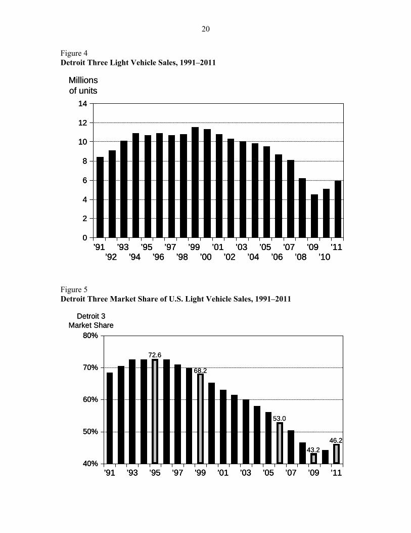
As shown in figure 4, U.S. sales of light vehicles6 by the Detroit Three peaked in
1999 at 11.5 million units, and then declined systematically thereafter until 2009, when
sales hit bottom at 4.5 million units. Total employment in the SEMCOG region, highly
correlated with Detroit Three sales, followed suit with a collapse of its own. Through
2005, the plummet in Detroit Three sales was almost solely due to a rapid decline in
market share, which shrank from 68.2 percent in 1999 to 53 percent in 2006, as shown in
figure 5. By the second half of the decade of the 2000s, total sales were in decline as
well, and that augmented the negative effects of a still-declining market share, which hit
bottom in 2009 at 43.2 percent.
6Light vehicles include cars, minivans, sport utility vehicles, crossovers, and pickup trucks.
20
Figure 4 Detroit Three Light Vehicle Sales, 1991–2011
Figure 5 Detroit Three Market Share of U.S. Light Vehicle Sales, 1991–2011
Millionsof units
0
2
4
6
8
10
12
14
’91 ’93 ’95 ’97 ’99 ’01 ’03 ’05 ’07 ’09 ’11’92 ’94 ’96 ’98 ’00 ’02 ’04 ’06 ’08 ’10
Millionsof units
0
2
4
6
8
10
12
14
0
2
4
6
8
10
12
14
’91 ’93 ’95 ’97 ’99 ’01 ’03 ’05 ’07 ’09 ’11’91 ’93 ’95 ’97 ’99 ’01 ’03 ’05 ’07 ’09 ’11’92 ’94 ’96 ’98 ’00 ’02 ’04 ’06 ’08 ’10’92 ’94 ’96 ’98 ’00 ’02 ’04 ’06 ’08 ’10
’91 ’93 ’95 ’97 ’99 ’01 ’03 ’05 ’07 ’09 ’11
Detroit 3Market Share
40%
50%
60%
70%
80%
53.0
43.2
46.2
72.6
68.2
’91 ’93 ’95 ’97 ’99 ’01 ’03 ’05 ’07 ’09 ’11’91 ’93 ’95 ’97 ’99 ’01 ’03 ’05 ’07 ’09 ’11
Detroit 3Market Share
40%
50%
60%
70%
80%
40%
50%
60%
70%
80%
53.0
43.2
46.2
72.6
68.2

21
Possibly the best single statistic to answer the “why” question on the retrenchment
of the Southeast Michigan economy is found in the market share numbers—those and
data on the concentration of the auto industry in the region, which remains off the charts.
The uptick in market share in 2010 and 2011, now at 46.2 percent, together with some
rebound in total sales, has opened the door for a moderately improving local economy.
Detroit Three sales came in at 5.9 million for 2011, and we see sales increasing slowly
for the next several years. Given that the average age of a vehicle on the road today is a
record 10.8 years old, replacement purchases will not likely be delayed much longer.
The revival in Detroit Three sales, albeit subdued so far, bodes well for the near-
term outlook for the region. In the longer term, we don’t view autos as a growth industry,
but past evidence shows that the local economy can expand so long as there is stability in
the sector, at least in an output sense. The prospects for employment in the auto industry,
and in manufacturing in general, are less favorable in our view, as we expect fairly robust
long-term productivity growth over time.
We now turn to a detailed analysis of our baseline economic and demographic
forecast for the SEMCOG region.
Forecast for Southeast Michigan through 2040
Current conditions locally as well as anticipated future trends nationally portend
growth, but only at a moderate pace, for Southeast Michigan’s population and labor
market over the next thirty years. This impression is confirmed by the results of our
demographic and economic forecast through 2040 for the seven-county SEMCOG
region. We should recognize from the outset that long-term forecasts are intended to
identify economic trends, not to predict movements in the business cycle. These

22
forecasts are also unable to capture major one-time events for which there is no prior
knowledge, such as a terrorist attack or an oil embargo. With these caveats in mind, we
now review the headline items for our regional forecast.
Demographics
We follow the pattern established by our schematics, and consider first our
forecast of the region’s population trajectory, which is central to the speed limits imposed
on local employment in the long run. The path of total population in the SEMCOG
region from 1990 to 2040 is shown in figure 6, with data from 1990 to 2010 provided by
the U.S. Bureau of the Census [5] and the extension through 2040 generated by our
forecast. Population in the region increased steadily from 4.59 million in 1990 to 4.89
million in 2004, and then began to decline, dropping to 4.71 million in 2010. The
population is forecast to continue to decline at a very modest rate over the next few years,
Figure 6 Population of SEMCOG Region, 1990–2040
4.5
4.6
4.7
4.8
4.9
5.0Millions
’90 ’95 ’00 ’05 ’10 ’15 ’20 ’25 ’30 ’35 ’404.5
4.6
4.7
4.8
4.9
5.0
4.5
4.6
4.7
4.8
4.9
5.0Millions
’90 ’95 ’00 ’05 ’10 ’15 ’20 ’25 ’30 ’35 ’40’90 ’95 ’00 ’05 ’10 ’15 ’20 ’25 ’30 ’35 ’40

23
reaching a low of 4.68 million in 2022. Population then expands slowly, reaching 4.76
million in 2040. According to our forecast, the relatively poor performance of the local
economy between 2001 and 2009 has resulted in a permanent loss of population.
These population movements are a product of natural change (births minus
deaths) and net migration patterns (international plus domestic migration), as illustrated
in schematic 1. The trajectory for total regional population through 2040 shown in
figure 6 is dissected by decade into its two component parts in figure 7. Even during the
prosperous 1990s, the SEMCOG region suffered a net loss of migrants (47,168), but the
excess of births over deaths (293,620) allowed the region to grow by almost a quarter of a
million people (–47,168 + 293,620 = 246,452).7 Between 2000 and 2010, however, the
Figure 7 Components of Population Change, SEMCOG Region, 1990–2040
7To reiterate, the natural increase in population reflected the difference in the number of births and deaths between July 1, 1990, and July 1, 2000. Net migration included both domestic and international groups.
–400
–300
–200
–100
0
100
200
300
400Thousands
1990–2000 2000–2010 2010–2020 2020–2030 2030–2040
=+ =+=+ =+ =+
Net migration Natural change in population
Total change in population
–400
–300
–200
–100
0
100
200
300
400
–400
–300
–200
–100
0
100
200
300
400Thousands
1990–2000 2000–2010 2010–2020 2020–2030 2030–2040
=+ =+=+ =+ =+
Net migration Natural change in populationNet migrationNet migration Natural change in populationNatural change in population
Total change in populationTotal change in population
24
region lost about 129,000 people, reflecting net out-migration of 340,229. If the rate of
natural population growth had not slowed to 211,188 but instead had remained the same
as during the 1990s, the population loss would have been only about 47,000.
The business cycle recovery after 2010 reduces the migration loss to 145,066
between 2010 and 2020, and cuts the aggregate population loss over the decade to about
23,000. Between 2020 and 2030, the region’s net migration mitigates to a loss of only
34,744. That is better than the migration statistics during the 1990s, but because births
exceed deaths by only 61,729, the region’s population barely expands.
In the decade after 2030, the region’s deaths exceed its births, but by a mere
7,421. Thus, the sole source of population growth after 2030 is net migration, especially
international migration. If the net migration to the region does not turn positive after
2030, as we are forecasting, the region’s population will shrink once again.
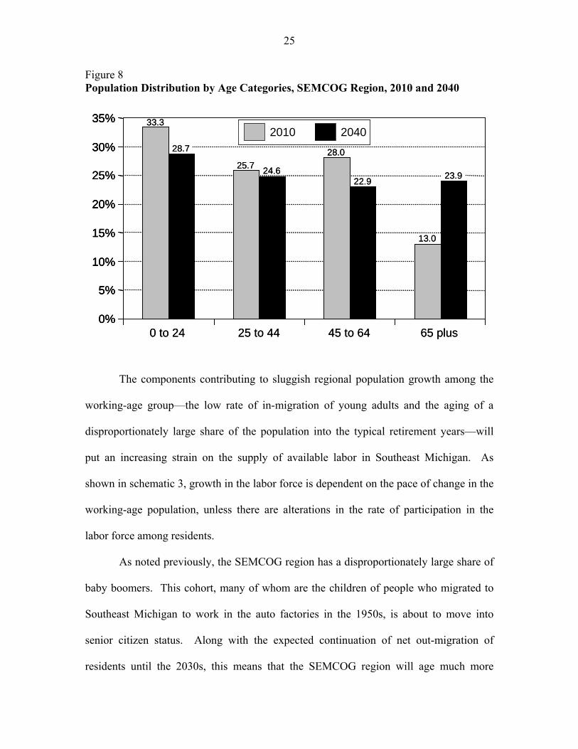
The aging of the baby boomer generation and the low rate of in-migration of
young adults, either foreign or domestic, results in a dramatic aging of the region’s
population. As shown in figure 8, the share of the population aged 65 or older is forecast
to increase from 13 percent in 2010, roughly one person in eight, to 23.9 percent in 2040,
almost one person in four. Correspondingly, the share of the population in cohorts under
65 shrinks. Children and college-age adults, those aged 24 and under, decline from 33.3
percent of the population today to 28.7 percent in 2040. The cohort now occupied by the
baby boomer generation, those aged 45 to 64, sees a fall in share from 28 percent to 22.9
percent over the period 2010–40. For a statistic where even a one- or two-point change is
notable, this represents a dramatic transformation in the age distribution of the region’s
population.
25
Figure 8 Population Distribution by Age Categories, SEMCOG Region, 2010 and 2040
The components contributing to sluggish regional population growth among the
working-age group—the low rate of in-migration of young adults and the aging of a
disproportionately large share of the population into the typical retirement years—will
put an increasing strain on the supply of available labor in Southeast Michigan. As
shown in schematic 3, growth in the labor force is dependent on the pace of change in the
working-age population, unless there are alterations in the rate of participation in the
labor force among residents.
As noted previously, the SEMCOG region has a disproportionately large share of
baby boomers. This cohort, many of whom are the children of people who migrated to
Southeast Michigan to work in the auto factories in the 1950s, is about to move into
senior citizen status. Along with the expected continuation of net out-migration of
residents until the 2030s, this means that the SEMCOG region will age much more
0%
5%
10%
15%
20%
25%
30%
35%
0 to 24 25 to 44 45 to 64 65 plus
2010 204033.3
28.7
25.724.6
28.0
22.9
13.0
23.9
0%
5%
10%
15%
20%
25%
30%
35%
0%
5%
10%
15%
20%
25%
30%
35%
0 to 24 25 to 44 45 to 64 65 plus
2010 20402010 204033.3
28.7
25.724.6
28.0
22.9
13.0
23.9

26
dramatically than the nation as a whole. Currently the region and the country have the
same share of the population aged 65 and older (13 percent), but over the next few years
they will diverge. By 2040, 23.9 percent of the SEMCOG region’s population will be 65
or older, compared with 19.6 percent nationwide (figure 9).
Figure 9 Population Distribution by Age Categories, U.S. vs. SEMCOG Region, 2040
Virtually every part of the country will age dramatically over the next thirty years,
but more so in Southeast Michigan. By 2040, the age gap between the SEMCOG region
and the rest of the country, as measured by the share of the population 65 and older, will
be about the same as it is today between Florida and the rest of the country.
Employment
The change in employment is equal to the change in the labor force, after
accounting for changes in the number of unemployed (schematic 4). Our forecast of total
0%
5%
10%
15%
20%
25%
30%
35%
0 to 24 25 to 44 45 to 64 65 plus
U.S. SEMCOG32.0
28.7
25.6 24.622.8 22.9
19.6
23.9
0%
5%
10%
15%
20%
25%
30%
35%
0%
5%
10%
15%
20%
25%
30%
35%
0 to 24 25 to 44 45 to 64 65 plus
U.S. SEMCOGU.S. SEMCOG32.0
28.7
25.6 24.622.8 22.9
19.6
23.9
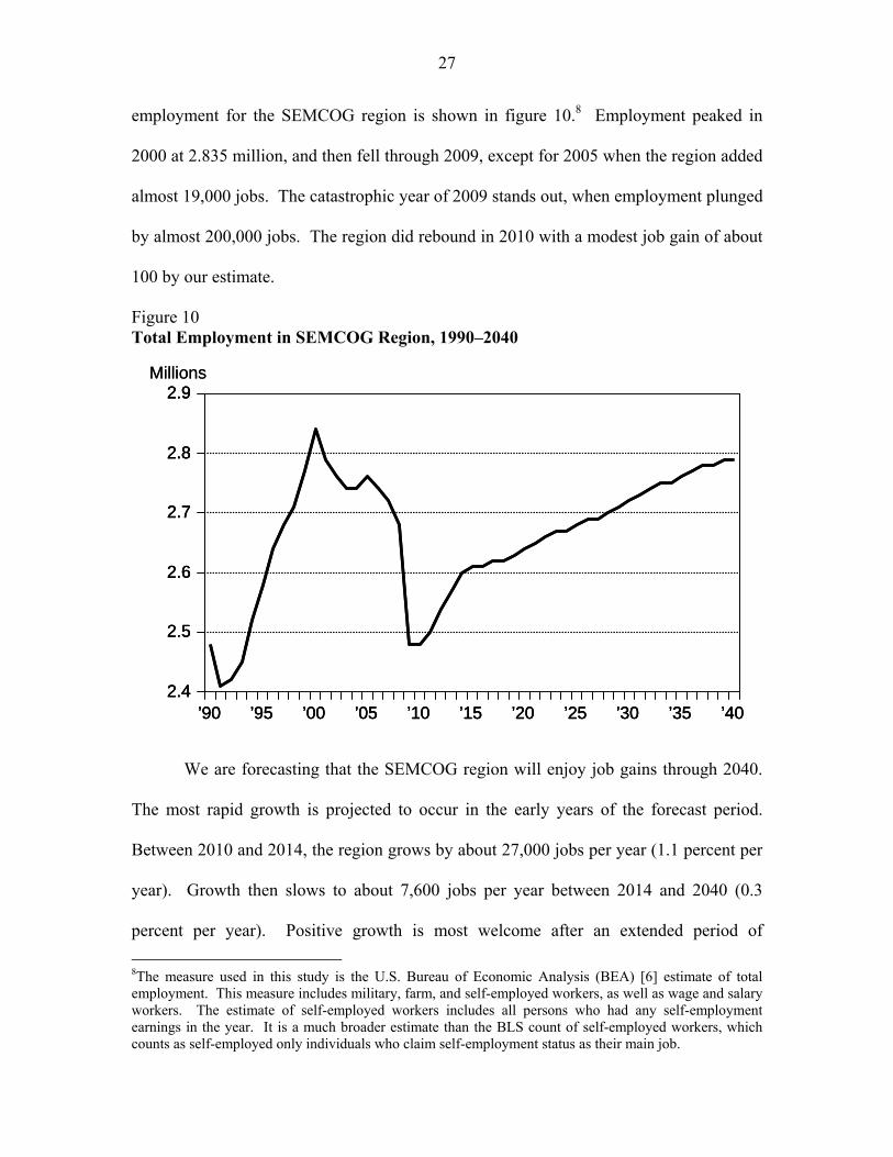
27
employment for the SEMCOG region is shown in figure 10.8 Employment peaked in
2000 at 2.835 million, and then fell through 2009, except for 2005 when the region added
almost 19,000 jobs. The catastrophic year of 2009 stands out, when employment plunged
by almost 200,000 jobs. The region did rebound in 2010 with a modest job gain of about
100 by our estimate.
Figure 10 Total Employment in SEMCOG Region, 1990–2040
We are forecasting that the SEMCOG region will enjoy job gains through 2040.
The most rapid growth is projected to occur in the early years of the forecast period.
Between 2010 and 2014, the region grows by about 27,000 jobs per year (1.1 percent per
year). Growth then slows to about 7,600 jobs per year between 2014 and 2040 (0.3
percent per year). Positive growth is most welcome after an extended period of
8The measure used in this study is the U.S. Bureau of Economic Analysis (BEA) [6] estimate of total employment. This measure includes military, farm, and self-employed workers, as well as wage and salary workers. The estimate of self-employed workers includes all persons who had any self-employment earnings in the year. It is a much broader estimate than the BLS count of self-employed workers, which counts as self-employed only individuals who claim self-employment status as their main job.
2.4
2.5
2.6
2.7
2.8
2.9Millions
’90 ’95 ’00 ’05 ’10 ’15 ’20 ’25 ’30 ’35 ’402.4
2.5
2.6
2.7
2.8
2.9
2.4
2.5
2.6
2.7
2.8
2.9Millions
’90 ’95 ’00 ’05 ’10 ’15 ’20 ’25 ’30 ’35 ’40’90 ’95 ’00 ’05 ’10 ’15 ’20 ’25 ’30 ’35 ’40

28
downturn, but the growth is not robust, so that by 2040, employment in the region still
remains slightly below the levels achieved in 2000.
The future path of employment in the region is, of course, the net result of the
outlooks for the industries that make up the local economy. Over the entire period 2010
to 2040, total employment is forecast to grow by an average of 0.39 percent per year in
the SEMCOG region, as shown in figure 11, with a wide variation in the performance of
the constituent industries. The strongest growth is in the private education and health
services industry category, dominated by the health care segment and expected to expand
at a rate of 1.14 percent per year. This industry has been the most robust over the past
difficult decade, and since we are on the threshold of a surge in the number of people
reaching retirement age, the longer-term prospects are very favorable as well. The
professional and business services category also sees comparatively rapid employment
growth of 0.85 percent per year.
Figure 11 Change in Employment by Industry, SEMCOG Region, 2010–40
Manuf.TTUGovt. FinanceProf.& Bus.
Ed. &Health
Leisure& Hosp.
Other
% ChangePer Year
– 0.8
– 0.6
– 0.4
– 0.2
0
0.2
0.4
0.6
0.8
1
1.2
1.4
Total jobs(0.39%)
1.14
0.85
0.31 0.280.19
0.10
– 0.15
– 0.54
Manuf.TTUGovt. FinanceProf.& Bus.
Ed. &Health
Leisure& Hosp.
Other
% ChangePer Year
– 0.8
– 0.6
– 0.4
– 0.2
0
0.2
0.4
0.6
0.8
1
1.2
1.4
– 0.8
– 0.6
– 0.4
– 0.2
0
0.2
0.4
0.6
0.8
1
1.2
1.4
Total jobs(0.39%)
Total jobs(0.39%)
1.14
0.85
0.31 0.280.19
0.10
– 0.15
– 0.54

29
At the other end of the spectrum is manufacturing, which declines on average by
0.54 percent per year.9 This does not mean that the output of local manufacturing firms
will decline; indeed, we are forecasting an increase in manufacturing output of 2.1
percent per year. But because productivity growth in manufacturing is relatively high—
we are forecasting that real output per employee will increase by 2.6 percent per year—
employment declines along with that pace of output growth.10
Employment is also forecast to decline in the trade, transportation, and utilities
sector over the next thirty years. The sector’s entire job loss is anticipated to occur in
trade and utilities, while the transportation industry adds jobs.
Modest job growth is projected for leisure and hospitality services, financial
activities, and government. Slightly faster growth is anticipated for the grab bag “other
industries” category, which includes farming and natural resources, construction,
information, and miscellaneous other services (largely personal and repair services).
Income
Income is another important dimension of the region’s economic profile.
Inflation-adjusted (real) personal income per capita is generally regarded by economists
as the best single measure of economic well-being for a region. The standard of living
for a region can rise even with sluggish employment growth if the incomes of residents
are rising sufficiently. The average annual growth in real personal income per capita for
9The manufacturing industry only includes jobs at production facilities. White-collar workers in pre-production, including research, development, design, and other engineering functions, are classified as professional services in our data from the federal government. Likewise, those at corporate headquarters are designated as headquarters employees. This is the case even if the employer is a manufacturing firm such as General Motors or Ford. 10For comparison, the local manufacturing sector saw productivity growth of 3.6 percent per year during the past two decades.

30
the SEMCOG region is shown in figure 12, with the period 1990 to 2040 broken out into
five-year increments.
Figure 12 Average Annual Growth in Inflation-Adjusted Personal Income Per Capita, SEMCOG Region, 1990–2040
In the first five years of the 1990s, real income per capita increased by an average
of 1.1 percent per year. The next five years, 1995 to 2000, were even stronger, with per
capita income growing by 2.6 percent per year. Those fat years were then followed by
the lean years of the 2000–10 period, when real income per capita actually declined. The
recovery from the Great Recession revives growth in per capita income, to a range of 2.3
to 2.5 percent per year in the 2010–20 period. The series then settles in to a more
sustainable pace of 1.5 percent per year in the 2020–40 period. It should be noted in
passing that it is difficult to forecast income growth with a high degree of accuracy; this
is the softest part of our overall forecast.
–1.0%
–0.5%
0%
0.5%
1.0%
1.5%
2.0%
2.5%
3.0%
’90-’95’95-’00
’00-’05’05-’10
’10-’15’15-’20
’20-’25’25-’30
’30-’35’35-’40
1.1
2.6
– 0.1
2.5
– 0.4
2.3
1.51.4
1.6 1.6
–1.0%
–0.5%
0%
0.5%
1.0%
1.5%
2.0%
2.5%
3.0%
–1.0%
–0.5%
0%
0.5%
1.0%
1.5%
2.0%
2.5%
3.0%
’90-’95’95-’00
’00-’05’05-’10
’10-’15’15-’20
’20-’25’25-’30
’30-’35’35-’40
’90-’95’95-’00
’00-’05’05-’10
’10-’15’15-’20
’20-’25’25-’30
’30-’35’35-’40
1.1
2.6
– 0.1
2.5
– 0.4
2.3
1.51.4
1.6 1.6

31
The baseline forecast we have reviewed in this section is our best estimate of
where Southeast Michigan goes from here if current trends continue. The prospects for
the regional economy would be less favorable if the auto situation turns uglier, and
prospects would be more favorable if we are able to emulate the Pittsburgh experience.
To understand more fully the implications of these possibilities, we have generated two
alternative scenarios to our baseline forecast, and we turn to that analysis now.
Alternative Forecast Scenarios
In choosing alternative scenarios to the baseline forecast, we settled on one
potential hot spot and one potential cold spot in our forecast that could alter the outlook
for the region in a meaningful way. As such, these alternative scenarios do not represent
outcomes that we judge to be most likely—the baseline forecast does that—but they do
explore possibilities we judge to be feasible if some of our assumptions are off the mark.
Another qualifier: the two scenarios should not be interpreted as confidence intervals, or
likelihood brackets, around our baseline forecast. They are simply as advertised:
alternative scenarios based on a modified set of assumptions.
The cold spot we explore is: What happens in Southeast Michigan if the auto
industry statewide suffers another period of rapid loss in employment similar, on a
percentage basis, to the one that occurred between 2000 and 2010? And the hot spot is:
What happens in Southeast Michigan if the region performs as well post-2012 as
Pittsburgh has done over recent history? In our opinion, both of these are instructive
scenarios to consider when assessing the prospects for the Southeast Michigan economy,
and we’ll examine each in turn.

32
Alternative Scenario 1: Regional Auto Industry Takes Another Big Hit
We estimate that in the year 2000 the SEMCOG region accounted for 15.9
percent of motor vehicle manufacturing employment in the United States.11 Over the
next five years, the industry lost jobs throughout the nation, but the largest loss occurred
in the SEMCOG region. By 2009, the region is estimated to have had 65,285 jobs in
motor vehicle manufacturing, or about 10.2 percent of all such jobs in the nation. The
economic recovery and the resulting increase in vehicle sales, along with the small
improvement in Detroit Three market share (see figures 4 and 5), leads to an increase in
industry employment in the region to 73,939 by 2012, or 11.3 percent of all motor vehicle
manufacturing jobs in the United States. Recent information suggests that the recovery in
motor vehicle jobs might be coming in somewhat stronger than this, but not enough so to
alter the scenario fundamentally.
After 2012, employment in motor vehicle manufacturing in the SEMCOG region
declines slowly in our baseline scenario, gravitating to 44,263 jobs in 2040. This would
amount to 10.0 percent of all motor vehicle manufacturing jobs in the United States.
In the first, and more pessimistic, alternative scenario, we explore what the
outcome would be in the SEMCOG region if the local auto industry went through another
round of rapid decline in employment along the lines of what occurred between 2000 and
2010. We set this repeat event to take place in the decade between 2020 and 2030.
Specifically, we calibrated the forecast so that the percentage decline in auto industry
employment in Michigan as a whole during the 2020 to 2030 period would be
approximately the same as the percentage decline that occurred in the state, by our
11The motor vehicle manufacturing industry is defined throughout this report to include NAICS industries 3361, 3362, and 3363.

33
estimate, during the 2000 to 2010 period, that is, a 58 percent decline in auto
manufacturing jobs statewide.
This translated into a somewhat larger hit in the SEMCOG region in the 2020 to
2030 period, a drop of 61 percent in auto industry jobs. An implication of this
perturbation is that the SEMCOG region’s share of U.S. motor vehicle manufacturing
employment declines during the decade of the 2020s from 11.2 percent to 4.8 percent,
rather than from 11.2 percent to 10.6 percent as in our baseline forecast. The results are
shown in figure 13, with the alternative forecast for vehicle manufacturing employment
in the SEMCOG region shown by the dotted line, and the baseline forecast path (solid
line) included for comparison.
Figure 13 Alternative Forecast of Employment in Motor Vehicle and Parts Manufacturing, SEMCOG Region, 2001–40
0
20,000
40,000
60,000
80,000
100,000
120,000
140,000
160,000
180,000
200,000
Baseline Additional loss of automanufacturing jobs
’05 ’10 ’15 ’20 ’25 ’30 ’35’01 ’400
20,000
40,000
60,000
80,000
100,000
120,000
140,000
160,000
180,000
200,000
0
20,000
40,000
60,000
80,000
100,000
120,000
140,000
160,000
180,000
200,000
Baseline Additional loss of automanufacturing jobs
BaselineBaseline Additional loss of automanufacturing jobsAdditional loss of automanufacturing jobs
’05 ’10 ’15 ’20 ’25 ’30 ’35’01 ’40’05 ’10 ’15 ’20 ’25 ’30 ’35’01 ’40

34
The main observation from this experiment is that with the much smaller base of
auto manufacturing jobs by 2020 than existed in 2000, the decline in auto jobs during the
2020s in the alternative scenario is much smaller in number compared with the job loss
we saw in the first decade of the 2000s. In the baseline run, the local motor vehicle
manufacturing industry is forecast to employ 52,904 workers by 2030, while under the
alternative scenario, employment would be 23,998, a shortfall of 28,906. This number
compares favorably with what we saw in the 2000–10 period, when the industry lost
almost five times as many jobs, with employment falling by 139,507 by our estimate. By
2040, the industry employment gap between the baseline run and the alternative scenario
shrinks to 23,367 workers, compared with the shortfall of 28,906 for 2030.
That even a repeat of the 2000–10 episode for the Detroit Three would have much
more modest negative employment effects on the region is illustrated for total local
employment in figure 14. Again, the employment path for the alternative scenario is
represented by the dotted line, and the baseline forecast path by the solid line. In this
case, the alternative path for total employment reflects the same perturbation of motor
vehicle manufacturing employment illustrated in the previous figure, but this time the
results include as well the spinoff job losses associated with the decline in auto jobs.
In the baseline forecast, employment in the region would reach 2.719 million by
2030. In the alternative scenario, total employment is estimated to be 2.583 million that
year, a net loss of 135,751 jobs (including the loss of 28,906 jobs in vehicle
manufacturing and 106,845 nonvehicle manufacturing spinoff jobs). By 2040, the loss in
the alternative scenario would shrink to 113,305 jobs, or 4 percent. The total number of
jobs in 2040 in the alternative scenario exceeds by 33,709 the level for 2020, that is, prior

35
to our imposition of job loss between 2020 and 2030 in the auto manufacturing industry.
In contrast, a similar loss, on a percentage basis, of auto manufacturing jobs during the
2000–10 period resulted in a major job hit, spurring a total loss of 350,905 jobs that are
not completely recovered by 2040 in our baseline forecast.
Figure 14 Alternative Forecasts of Total Employment (Auto scenario), SEMCOG Region, 2001–40
Alternative Scenario 2: Growing Like Pittsburgh
For the second, and more optimistic, alternative scenario, we model what the
SEMCOG region would look like if it performed after 2012 as well as Pittsburgh has
done over recent history. As mentioned previously, Pittsburgh is often held up as the
standard to reach for by regions hard hit by structural change and that are striving for a
revitalized economy. Between 1986 and 2009, employment in the Pittsburgh Combined
Statistical Area (CSA) grew at 60 percent of the U.S. growth rate (0.84 percent per year
Millions
’05 ’10 ’15 ’20 ’25 ’30 ’35’01 ’402.4
2.5
2.7
2.8
2.9
2.6
Baseline
Total job loss with autoindustry retrenchment
Millions
’05 ’10 ’15 ’20 ’25 ’30 ’35’01 ’40’05 ’10 ’15 ’20 ’25 ’30 ’35’01 ’402.4
2.5
2.7
2.8
2.9
2.6
2.4
2.5
2.7
2.8
2.9
2.6
Baseline
Total job loss with autoindustry retrenchment
BaselineBaseline
Total job loss with autoindustry retrenchmentTotal job loss with autoindustry retrenchment

36
compared with 1.40 percent).12 So, in this alternative scenario, we adjust the forecast to
ensure that employment in the Detroit CSA (a somewhat larger area than the SEMCOG
region) grows at 60 percent of the U.S. growth rate between 2012 and 2040.13
As shown in figure 15, where we continue the convention of displaying the
alternative scenario with a dotted line and the baseline forecast with a solid line, the result
of our perturbation is somewhat more rapid employment growth in the SEMCOG region.
If employment in the region were to match Pittsburgh’s recorded performance, its level
by 2040 would be 2.941 million instead of the 2.789 million generated in our baseline
forecast—a gain of about 152,000 jobs, or 5 percent.
Figure 15 Alternative Forecasts of Total Employment (“Like Pittsburgh” scenario), SEMCOG Region, 2001–40
12See footnote 4 for the definition of the Pittsburgh region used in this report. 13In addition to the seven-county SEMCOG region, the Detroit CSA includes Genesee and Lapeer counties.
2.4
2.5
2.6
2.7
2.8
2.9
3.0
Millions
’05 ’10 ’15 ’20 ’25 ’30 ’35’01 ’40
Baseline
Extra gain in “Like Pittsburgh” jobs
2.4
2.5
2.6
2.7
2.8
2.9
3.0
Millions
2.4
2.5
2.6
2.7
2.8
2.9
3.0
Millions
’05 ’10 ’15 ’20 ’25 ’30 ’35’01 ’40’05 ’10 ’15 ’20 ’25 ’30 ’35’01 ’40
Baseline
Extra gain in “Like Pittsburgh” jobs
BaselineBaseline
Extra gain in “Like Pittsburgh” jobsExtra gain in “Like Pittsburgh” jobs

37
Under this alternative scenario, the region’s employment in 2040 would exceed its
2000 peak level by about 106,000 jobs. Thus, the region would certainly benefit from
following in Pittsburgh’s footsteps, but the benefits would take a very long time to
accrue.
For illustrative purposes, we have consolidated the effects on total employment of
the two alternative scenarios, together with the baseline forecast (solid line), in a single
display, figure 16. Obviously, any comparisons between the auto (dashed line) and
Pittsburgh (dotted line) scenarios are shaped by the scale and timing we settled on to
design the two experiments. With that qualifier in mind, the outcomes for the two
alternatives trace out a relatively small range of difference in impact considering the large
variance in the events—total employment by 2040 of 2.675 million in the more
pessimistic scenario and 2.941 million in the more optimistic alternative.
Figure 16 Alternative Forecasts of Total Employment (Autos and “Like Pittsburgh”), SEMCOG Region, 2001–40
2.4
2.5
2.6
2.7
2.8
2.9
3.0
Millions
’05 ’10 ’15 ’20 ’25 ’30 ’35’01 ’40
Baseline
Extra gain in “Like Pittsburgh” jobs
Total job loss with autoindustry retrenchment
2.4
2.5
2.6
2.7
2.8
2.9
3.0
Millions
2.4
2.5
2.6
2.7
2.8
2.9
3.0
Millions
’05 ’10 ’15 ’20 ’25 ’30 ’35’01 ’40’05 ’10 ’15 ’20 ’25 ’30 ’35’01 ’40
Baseline
Extra gain in “Like Pittsburgh” jobs
Total job loss with autoindustry retrenchment
BaselineBaseline
Extra gain in “Like Pittsburgh” jobsExtra gain in “Like Pittsburgh” jobs
Total job loss with autoindustry retrenchmentTotal job loss with autoindustry retrenchment

38
The caution issued at the beginning of this section bears repeating here: this range
is not intended to represent a confidence interval around our baseline forecast. Instead,
the dashed and dotted lines simply represent two different scenarios that we consider
feasible, but less likely than our baseline forecast.
Looming Labor Shortages
We raised the issue earlier of where the supply of workers will come from in the
decades to come. The schematics in the third section of the report identify an exhaustive
list of the potential sources of labor:
1. Increases in the working-age population as young residents come of age
2. Increases in net in-migration of the working-age cohort
3. Increases in the labor force participation rate of current residents14
4. Drawing from the unemployed
Our forecast and its underlying architecture suggest that the number of additional
workers from any of these sources will be severely limited. The fundamental problem, of
course, is the rapid aging of the population over the next thirty years. According to our
forecast (figure 8), the share of SEMCOG’s population aged 65 or older will increase
from 13 percent in 2010 to 23.9 percent in 2040—a much more dramatic aging profile
than in the nation as a whole. Sluggish population growth among SEMCOG’s working-
age group stems from a dramatic slowing (and after 2030, a decline) in natural population
growth with the aging of the population, and the low rate of in-migration of young adults
that we anticipate (the first two sources of labor listed above, and shown in figure 7).
14Examples of people not participating would be those who do not work outside of the home, retirees, full-time students, or those on welfare.

39
One factor that could compensate somewhat for weak growth in the working-age
population would be increases in the labor force participation rate, identified above as the
third source of labor. In our forecast, we are estimating a fairly large increase in
participation rates across each age category, ranging from a two-percentage-point
increase to an eleven-percentage-point increase from 2010 to 2040. For example, in the
30 to 34 age category, we see an increase in the rate from 79.0 percent in 2010 to 83.7
percent in 2040; in the 65 to 69 age category, we project an increase from 26.8 percent to
37.9 percent over the period.
Even though every individual age component shows an increase, however, the
labor force participation rate overall falls from 60.5 percent in 2010 to 57.8 percent in
2040. How so? Because the total participation rate is a weighted average of the rates
across age groups, and over time the older cohorts with the lowest rates gain significantly
in their proportion of the population. Indeed, if we are off the mark here, it is more likely
that we have been too generous on the increases in participation rates among the age
cohorts, suggesting that labor supply could be even more squeezed from this source.
The last source of labor supply listed above is drawing from the unemployed, but
in our forecast we have assumed a low and stable unemployment rate approaching an
equilibrium position over the period, leaving little room to add workers from this source.
So, among the four sources of labor supply listed above, where is the potential to
squeeze out significantly greater numbers of workers? Realistically, there is only one:
the trends most subject to influence would be the migration rates. Employment
opportunities are the strongest magnet for these people, but educational opportunities,
quality of life, and family ties also matter. Otherwise, the labor supply constraints

40
outlined here ultimately impose a serious speed limit on economic growth. The prospects
for labor shortages in the future, particularly of workers with skills that mesh with the
emerging knowledge- and information-based economy, is an issue that should be on our
radar screen today.
Conclusion
So, where does this leave us? We appear to be emerging from the tunnel that was
the most catastrophic period for the Southeast Michigan economy in our lifetime. The
tunnel was frightening—during the first decade of the 2000s, the region lost virtually all
of the jobs gained in the robust growth decade of the 1990s—and seeing daylight ahead is
refreshing, but in fact are we actually leaving the tunnel? And if so, are we going to
traverse the same landscape as before?
On the first question, the near-term outlook, there does appear to be growing
evidence that the economy of Southeast Michigan, and for that matter Michigan in
general, is returning to positive growth. This observation is supported by the recent flow
of data releases, in news reports, and by our forecast of the local economy contained in
this report. Growth is more subdued, however, than what is commonly expected coming
out of a recession. The local economy is far from being back to normal, and many
residents will not be vested in the recovery for some time to come. But the region has
made a good start, its competitive position turned around after 2009, and we see job
growth being sustained. So, our answer to the first question is, yes, we are leaving the
tunnel.
On the second question, the longer-term outlook, the answer is no, we won’t be
traveling the same route as before after exiting the tunnel. We see long-term growth to
41
be sure, but only at a moderate pace for Southeast Michigan’s population and labor
market over the next thirty years, much more subdued than what transpired in the 1990s
prior to the extended downturn. And growth is more muted going forward than we
anticipated several years ago—now our view is that by 2040 the region’s employment
will still remain slightly below its peak level achieved in 2000. One consequence of the
poor performance of the local economy between 2000 and 2009 is a permanent loss of
population and a deep hole for the economy to dig out of. On the demand side, we don’t
see especially strong growth nationally and we don’t view the region’s dominant sector,
the domestic automotive industry, as a long-term growth sector, particularly in terms of
employment given the solid productivity gains we anticipate.
The bigger issue is on the supply side. Population is central to the speed limits
imposed on local employment in the long run. If, over the longer term, unemployment
and labor force participation settle in at fairly stable rates, work force gains would largely
need to come from increases in the working-age population, which in turn would derive
from young residents becoming of working age or from net in-migration. But because
the SEMCOG region has a disproportionately large share of baby boomers, it will age
much more dramatically than the nation as a whole. By 2040, the age gap between the
region and the rest of the country, as measured by the share of the population 65 and
older, will be about the same as it is today between Florida and the rest of the country.
That leaves net in-migration, which has typically been low for young adults and who to
date have not altered the region’s profile in a meaningful way. It’s hard to fathom in our
current high unemployment environment, but the looming problem down the road will be

42
labor shortages, particularly of workers with skills that mesh with the evolving
knowledge- and information-based economy.
The hope, of course, is that the retrenchment the region has suffered through can
also be the precursor to an era of renewal. Our policy prescription remains the same as
the last time we engaged in this exercise: investment in a more highly skilled and
educated work force, and retention of greater numbers of our high-income retirees. Our
forecast and the underlying data suggest that there are challenges that need to be
addressed, but the Southeast Michigan region has the assets, the wherewithal, and the
motivation to get there. Again, we remain optimistic that we can and will do better.

43
References
1. Crary, Joan P., and Fulton, George A. “The Michigan Economic Outlook.” Ann Arbor: Research Seminar in Quantitative Economics, University of Michigan. Updated quarterly.
2. Regional Economic Models, Inc. http://www.remi.com/
3. Treyz, George I. Regional Economic Modeling: A Systematic Approach to Economic Forecasting and Policy Analysis. Boston: Kluwer Academic Publishers, 1993.
4. Treyz, George I.; Rickman, Dan S.; and Shao, Gang. “The REMI Economic-Demographic Forecasting and Simulation Model.” International Regional Science Review 14, no. 3 (1992):221–53.
5. U.S. Bureau of the Census. http://www.census.gov/
6. U.S. Bureau of Economic Analysis. http://www.bea.gov/
7. U.S. Bureau of Labor Statistics, Quarterly Census of Employment and Wages. http://www.bls.gov/

44
About the Authors
Donald R. Grimes holds a master’s degree in Economics from the University of Michigan. He is a senior research specialist at the University of Michigan’s Institute for Research on Labor, Employment, and the Economy. His primary research interests are in labor economics and economic forecasting.
For the past two decades, he has worked on forecasting labor market activity in the metropolitan areas of Michigan. He has worked for many years with the Michigan departments of Commerce and Treasury and the Michigan Economic Development Corporation on policy analysis and evaluating economic strategies. He has also participated in economic studies designed to assist firms in their location and expansion decisions. He is co-director of a project to generate long-term economic and demographic projections for all of the counties of Michigan. He has been involved in other research projects sponsored by the U.S. Department of Commerce, the U.S. Department of Labor, the Federal Reserve Bank of Chicago, and the Robert Wood Johnson Foundation.
Among his publications, he has co-authored a paper on the changing concentration of computer service industry employment, “Change in the Concentration of Employment in Computer Services: Spatial Estimation at the U.S. Metro County Level” (Growth and Change, March 2007). He also co-authored a chapter on the location of technology firms in Michigan at the Millennium.
George A. Fulton received his Ph.D. in economics from the University of Michigan. He is currently the director of the Research Seminar in Quantitative Economics in the Department of Economics at the University of Michigan. He also holds an appointment as research professor at the University’s Institute for Research on Labor, Employment, and the Economy, where he is director of the Center for Labor Market Research.
Dr. Fulton has been forecasting economic and fiscal activity in the state of Michigan for over three decades. In addition, he is co-director of a project to generate long-term economic and demographic projections for all the counties of Michigan. He is a principal advisor to the University administration and to the state government on the economic situation in Michigan. He has written a book on the Michigan regional economies, co-authored with former University of Michigan President Harold T. Shapiro. His research crosses disciplines, having been published in diverse professional journals and sponsored research reports.