The economic contribution of Melbourne’s foodbowl A report for the Foodprint Melbourne project, University of Melbourne

July 2016

Contents Key points ........................................................................................................................ i

Executive Summary ......................................................................................................... ii

1 Introduction .......................................................................................................... 1

2 Profile of Melbourne’s foodbowl ........................................................................... 2

2.1 Melbourne’s foodbowl........................................................................................... 2

2.2 Agricultural production in the foodbowl ................................................................. 3

2.3 Food manufacturing activities ................................................................................ 6

2.4 Food consumption in Melbourne ........................................................................... 7

3 Economic contribution of Melbourne’s foodbowl ................................................ 12

3.1 Methodology ....................................................................................................... 12

3.2 Results ................................................................................................................. 13

4 Economic impacts under alternative future scenarios.......................................... 15

4.1 Methodology ....................................................................................................... 15

4.2 Melbourne growing to accommodate 7 million people ......................................... 16

4.3 Increasing preference for ‘local’ food ................................................................... 22

5 Ancillary benefits................................................................................................. 24

5.1 Insurance and option value .................................................................................. 24

5.2 Visual amenity ..................................................................................................... 25

5.3 Other ancillary benefits ........................................................................................ 26

5.4 Future ancillary benefits ...................................................................................... 27

5.5 Note on ancillary benefits .................................................................................... 28

6 Conclusion .......................................................................................................... 29

Appendix A Input-Output analysis ................................................................................. 31

Appendix B CGE modelling ............................................................................................ 33

Appendix C Local Sourcing assumptions ........................................................................ 37

References ..................................................................................................................... 38

Limitation of our work .................................................................................................... 41

Charts Chart 2.1 Victorian agricultural land, by region ................................................................ 4

Chart 2.2 Value of Agricultural Production in Melbourne’s foodbowl, by LGA .................. 4

Chart 2.3 Gross value of agricultural production in Melbourne’s foodbowl...................... 5

Chart 2.4 Persons employed in agriculture in the foodbowl, food production only .......... 6

Chart 2.5 Employment in selected food processing industries, by region ......................... 6

Chart 2.6 Average daily dietary intake, by food category ................................................. 8

Chart 2.7 Population of Greater Melbourne, 2011 to 2051 .............................................. 9

Chart 2.8 Melbourne’s food demand now and in future (thousand tonnes) ................... 10

Tables Table 2.1 : Definition of foodbowl areas .......................................................................... 2

Table 3.1 Economic contribution of agriculture and food manufacturing in Melbourne’s foodbowl ...................................................................................................................... 13

Table 3.2 Sectoral economic contribution in Melbourne’s foodbowl ............................. 14

Table 4.1 Assumptions under alternative growth scenarios ........................................... 16

Table 4.2 Share of population growth to 2031 in new residential areas ......................... 17

Table 4.3 Agricultural land and production in 7 growth local government areas ............ 18

Table 4.4 Sectoral impacts of ‘constrained urban sprawl’ .............................................. 18

Table 4.5 Sectoral impacts of ‘moderate urban sprawl’ ................................................. 20

Table C.1 Local sourcing assumptions ............................................................................ 37

Figures Figure 2.1 Map of Melbourne’s foodbowl........................................................................ 3

Figure 4.1 The components of DAE-RGEM and their relationships ................................. 15

Figure A.1 Input-output diagram ................................................................................... 31

i

Key points The value of Melbourne’s foodbowl to the regional economy is significant

Melbourne’s foodbowl accounts for more than 1.7 million hectares of agricultural land, consisting of a mix of enterprises, most notably vegetables, poultry, dairy and livestock production.

It contributes $2.45 billion per annum to the regional economy of Melbourne.

The value under future scenarios

Melbourne’s urban development affects the value of the foodbowl in two ways - less agricultural land leads to lower supply of food, at the same time a growing Melbourne leads to higher food demand. Both mechanisms will drive food prices higher.

The threat to the value of the foodbowl from urban development is significant. Under a future of Melbourne at 7 million people, some loss of agricultural land to urban development is expected and the value of annual agricultural output is modelled to fall by between $32 million and $111 million, with higher fresh food prices.

A continuation of a recent trend towards preferring more local sources of food increases the value of food production from the foodbowl. Under a scenario where consumers in Melbourne’s foodbowl increase their consumption of local food by a modest amount of 10%, the value of annual agricultural output from the foodbowl is modelled to be $290 million higher per annum.

The ancillary benefits of Melbourne’s foodbowl beyond these quantitative metrics include the insurance value against drought and climate change, the green wedge values associated with land used for farming rather than urban development, and the option value of land use that is retained when land is used for farming.

ii

Executive Summary Melbourne is Australia’s second largest city, with a population of around 4.6 million people.1 The area surrounding Melbourne’s urban fringe, or peri-urban area, is also one of the most productive agricultural regions in Victoria. It produces a variety of foods, especially a significant amount of fresh vegetables.

As Melbourne has grown, so too has its demand for food. However, growth in Melbourne’s population and industrial base has largely been accommodated by reducing the amount of land available for food production. This food paradox of urbanisation – that urbanisation simultaneously drives local demand for food higher and local production lower – is symbolic of the challenge of food production in an increasingly urbanised world. The traditional model of Melbourne’s urban development has clearly prioritised residential uses over food production in the peri-urban fringe.

Yet, the loss of farmland in Melbourne’s foodbowl to urban development is not inevitable, at least to the extent it has been lost in the past. Cities have choices over how to grow, and where. Making the right choices depends on having good information on the value of land use for different purposes, such as housing, food production or public open space.

Deloitte Access Economics has been engaged by the Victorian Eco-Innovation Lab at the University of Melbourne to undertake an economic analysis of the value of one of those land uses – the use of land to grow food.

The purpose of this project is to provide an assessment of the value of agriculture and related value-adding activities in Melbourne’s foodbowl, both now and in the future under different urban development and consumer food preference scenarios

The current economic contribution of agriculture and food processing in Melbourne’s foodbowl

Deloitte Access Economics estimates that the existing economic contribution of agriculture and related food manufacturing in Melbourne’s foodbowl is $2.45 billion per annum to gross regional product (GRP), and 21,001 full-time equivalent (FTE) jobs. This represents 0.84% of the entire Melbourne regional economy, and 1.06% of its work force. It is important to note that these are on-going annual contributions, not one-off impacts.

This total contribution is a function of three types of contribution that food grown in the region contributes to the regional economy, as follows:

1 Source: Victoria in Future (2015), Greater Melbourne Capital City Statistical Area as at 30 June 2016

iii

Direct contribution in the agriculture sector (on-farm activity and employment): the agriculture sector directly contributes approximately $956 million per annum in value-added terms to the regional economy and employs 7,687 people on a full time equivalent (FTE) basis.

Upstream indirect contribution, reflecting expenditure on inputs into foodbowl agriculture, generates $742 million per annum in value-added terms, and creates 5,719 FTEs in those upstream sectors.

Downstream food manufacturing in the region, attributable to agricultural produce grown within the foodbowl, contributes a further $756 million per annum to the regional economy and employs 7,595 FTEs directly.

Of the agricultural sectors, fruit and vegetables are the largest contributor to the regional economy in terms of direct value-added ($413 million) and direct employment (2,997 FTE jobs).

The potential impact of urban sprawl on Melbourne’s foodbowl

As Melbourne grows and land use changes from agricultural production to urban development, a reduction in agricultural land leads to a reduction in agricultural output and an increase in farmgate prices of agricultural products (because of the higher demand and reduced supply), with flow-on effects to the rest of the economy. Deloitte modelled two separate urban sprawl scenarios reflecting land use transition from agricultural production to urban development to accommodate a population of 7 million people:

1. A constrained urban sprawl scenario, where the food producing area in the foodbowl is reduced by 10,897 ha, or 0.62% of total food producing land in the foodbowl. The reduction in agricultural land is to accommodate the population growth, assuming an aspirational infill rate of 79%.

2. A moderate urban sprawl scenario, where the food producing area is reduced by 33,730 ha, or 1.92% of total food producing land in the foodbowl. The reduction in agricultural land is to accommodate the population growth, assuming an aspirational infill rate of 61%.

These two scenarios were modelled and compared with a ‘base case’, which reflects the current land use and agricultural production profile of Melbourne’s foodbowl. In order to isolate the effects of the changes in land use, population (which drives food demand) in these two scenarios and in the baseline is held constant at 7 million people.

In the constrained urban sprawl scenario of 0.62% less food producing area, annual agricultural output falls by $32 million (over $10 million of value-add) while employment falls by 70 FTEs (full time equivalents). Under the moderate urban sprawl scenario of 1.92% less food producing area, agricultural production falls by $111 million (around $37 million of value-add) while agricultural employment falls by 217 FTEs. As a result of declining

iv

agricultural output in both scenarios, there are flow-on effects to the rest of the economy in the foodbowl area, particularly in the food manufacturing sector. The flow-on effects are larger in the moderate urban sprawl scenario than in the constrained urban sprawl scenario.

The potential impact of a stronger preference for locally-sourced food in Melbourne

The change in preference of consumers in Melbourne’s foodbowl modelled by Deloitte was an increase in demand for locally grown food within the foodbowl. While there is a clear lack of data in this area, research suggests that Melbourne’s consumers have only some preference for food grown locally over food grown elsewhere. This ‘buy local’ preference is stronger for some agricultural commodities (e.g. perishable horticulture) than others.

Should this preference for locally grown food increase by 10% for most fresh commodities, annual agricultural output would increase by $290 million (around $131 million of value-add) and agricultural employment would increase by 1,183 FTEs, reflecting a supply response to this higher level of demand. The farmgate price received by agricultural producers in the foodbowl would increase by 5.3%, reflecting the higher value that consumers place on locally produced food over food produced elsewhere.

Ancillary benefits of retaining peri-urban land for agriculture

The economic figures only capture some of the value of retaining peri-urban land for agriculture. Ancillary benefits to keeping such land undeveloped include:

the insurance value against drought and climate change (and its associated impact on food prices) that can come through rainfall independent sources of irrigated agricultural production, made possible where treated recycled waste water from Melbourne is used for food production in the foodbowl;

the green wedge values associated with land used for farming rather than urban development, such as visual amenity, water quality and options for biodiversity (reflecting that there are more options for biodiversity on farmland than there are in built up areas);

the option value of land use that is retained when land is used for farming, but is lost when land is developed (once built upon, land is rarely returned as farmland or open space).

Agricultural production, especially vegetable production, in Melbourne’s foodbowl contributes significantly to the regional economy. The findings of this report will together outline a value proposition for using Melbourne’s foodbowl for food production. On its own, this will not provide or imply particular recommendations regarding alternative land use around Melbourne, but will provide some of the necessary inputs to the land use debate.

Deloitte Access Economics

1

1 Introduction The Victorian Eco-Innovation Lab at the University of Melbourne has engaged Deloitte Access Economics to undertake an economic analysis that will support Part 3 of the Foodprint Melbourne project. Foodprint Melbourne is a collaborative project between the Victorian Eco-Innovation Lab (University of Melbourne), Deakin University and Sustain: The Australian Food Network. It is a research project that investigates Melbourne’s foodbowl, the food growing area on Melbourne’s peri-urban fringe.

There are three parts to the Foodprint Melbourne project. Part 1 investigated the capacity of Melbourne’s foodbowl to feed Greater Melbourne now and in future. In Part 2, the environmental foodprint of feeding Greater Melbourne was investigated. In particular, the amount of land and water that it takes to feed the city, as well as associated waste and GHG emissions was quantified. Potential vulnerabilities in Melbourne’s food supply and approaches to address them were also identified.

As a component in Part 3 of Foodprint Melbourne, the purpose of this study is to deliver an analysis of the economic benefits of Melbourne’s foodbowl now and in the future. The focus of the study is to identify:

the current economic contribution of Melbourne’s foodbowl;2

the economic impacts of planning decisions to preserve agricultural land while accommodating population growth to 7 million people; and

the economic impact of an increase in demand for locally-grown food from consumers living in Melbourne’s foodbowl.

The current economic contribution of Melbourne’s foodbowl was estimated using Deloitte Access Economics’ Input-Output (IO) model while the Deloitte Access Economics’ Computable General Equilibrium model (DAE-RGEM) was used to estimate the economic impacts of future scenarios.

The rest of the report is organised as follows:

Chapter 2 presents the profiling of Melbourne’s foodbowl – geographical boundary, the value of production and employment in agriculture and food manufacturing, and the demand for food production from the foodbowl

Chapter 3 outlines the IO modelling methodology and details the current economic contribution

Chapter 4 describes the CGE modelling methodology and discusses the economic impacts under two alternative scenarios

Chapter 5 presents a discussion on ancillary benefits that are not captured in the modelling

Chapter 6 provides some concluding comments.

2 The spatial boundary of Melbourne’s foodbowl is defined in chapter 2.

2

2 Profile of Melbourne’s foodbowl This chapter provides a summary and profile of Melbourne’s foodbowl in terms of primary agricultural production, secondary processing and food demand of its growing population.

Publicly available data from the Australian Bureau of Statistics (ABS) was used to profile Melbourne’s foodbowl throughout this chapter. In particular, statistics reflect data collected in the Australian ABS Census of Population and Housing and the Agricultural Census, both of which last occurred in 2011. Because of this, 2011 is the latest year for which data is available.

2.1 Melbourne’s foodbowl

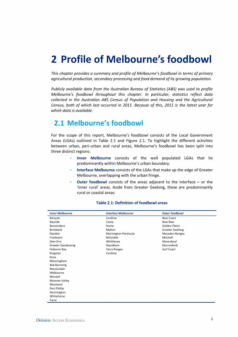
For the scope of this report, Melbourne’s foodbowl consists of the Local Government Areas (LGAs) outlined in Table 2.1 and Figure 2.1. To highlight the different activities between urban, peri-urban and rural areas, Melbourne’s foodbowl has been split into three distinct regions:

• Inner Melbourne consists of the well populated LGAs that lie predominantly within Melbourne’s urban boundary.

• Interface Melbourne consists of the LGAs that make up the edge of Greater Melbourne, overlapping with the urban fringe.

• Outer foodbowl consists of the areas adjacent to the interface – or the ‘inner rural’ areas. Aside from Greater Geelong, these are predominantly rural or coastal areas.

Table 2.1: Definition of foodbowl areas

Inner Melbourne Interface Melbourne Outer foodbowl

Banyule Cardinia Bass Coast Bayside Casey Baw Baw Boroondara Hume Golden Plains Brimbank Melton Greater Geelong Darebin Mornington Peninsula Macedon Ranges Frankston Nillumbik Mitchell Glen Eira Whittlesea Moorabool Greater Dandenong Wyndham Murrindindi Hobsons Bay Yarra Ranges Surf Coast Kingston Cardinia Knox Manningham Maribyrnong Maroondah Melbourne Monash Moonee Valley Moreland Port Phillip Stonnington Whitehorse Yarra

3

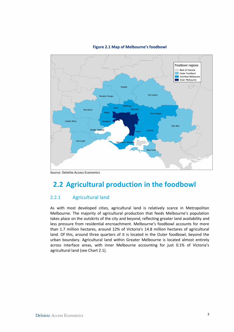
Figure 2.1 Map of Melbourne’s foodbowl

Source: Deloitte Access Economics

2.2 Agricultural production in the foodbowl

2.2.1 Agricultural land

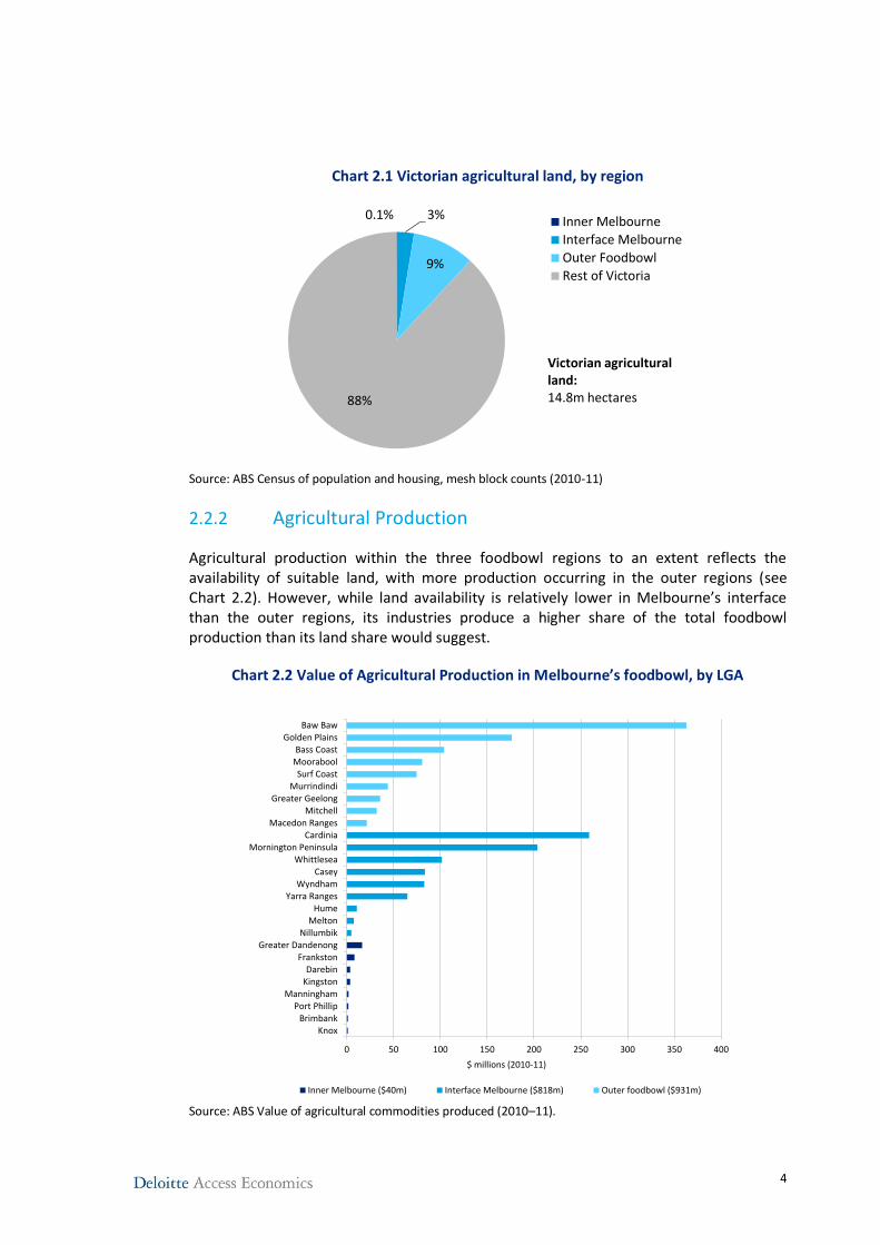
As with most developed cities, agricultural land is relatively scarce in Metropolitan Melbourne. The majority of agricultural production that feeds Melbourne’s population takes place on the outskirts of the city and beyond, reflecting greater land availability and less pressure from residential encroachment. Melbourne’s foodbowl accounts for more than 1.7 million hectares, around 12% of Victoria’s 14.8 million hectares of agricultural land. Of this, around three quarters of it is located in the Outer foodbowl, beyond the urban boundary. Agricultural land within Greater Melbourne is located almost entirely across interface areas, with inner Melbourne accounting for just 0.1% of Victoria’s agricultural land (see Chart 2.1).

4

Chart 2.1 Victorian agricultural land, by region

Source: ABS Census of population and housing, mesh block counts (2010-11)

2.2.2 Agricultural Production

Agricultural production within the three foodbowl regions to an extent reflects the availability of suitable land, with more production occurring in the outer regions (see Chart 2.2). However, while land availability is relatively lower in Melbourne’s interface than the outer regions, its industries produce a higher share of the total foodbowl production than its land share would suggest.

Chart 2.2 Value of Agricultural Production in Melbourne’s foodbowl, by LGA

Source: ABS Value of agricultural commodities produced (2010–11).

0.1% 3%

9%

88%

Inner Melbourne

Interface Melbourne

Outer Foodbowl

Rest of Victoria

Victorian agricultural land:14.8m hectares

0 50 100 150 200 250 300 350 400

KnoxBrimbank

Port PhillipManningham

KingstonDarebin

FrankstonGreater Dandenong

NillumbikMelton

HumeYarra Ranges

WyndhamCasey

WhittleseaMornington Peninsula

CardiniaMacedon Ranges

MitchellGreater Geelong

MurrindindiSurf Coast

MooraboolBass Coast

Golden PlainsBaw Baw

$ millions (2010-11)

Inner Melbourne ($40m) Interface Melbourne ($818m) Outer foodbowl ($931m)

5

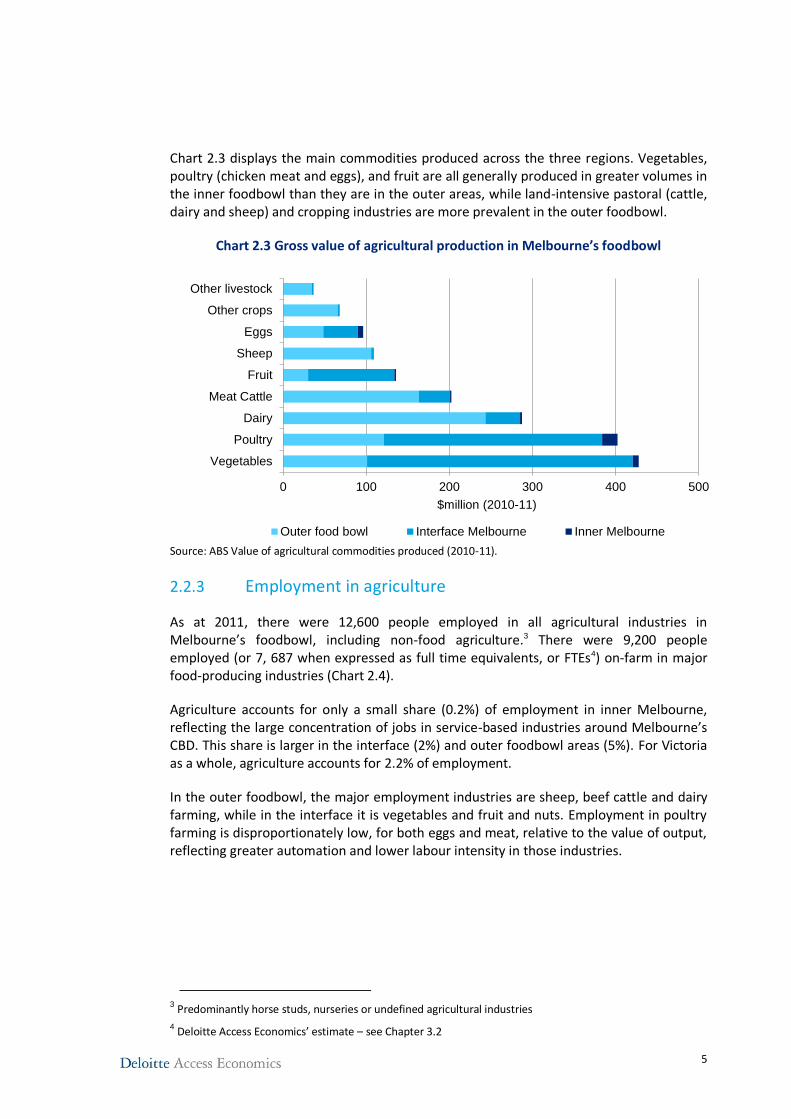
Chart 2.3 displays the main commodities produced across the three regions. Vegetables, poultry (chicken meat and eggs), and fruit are all generally produced in greater volumes in the inner foodbowl than they are in the outer areas, while land-intensive pastoral (cattle, dairy and sheep) and cropping industries are more prevalent in the outer foodbowl.

Chart 2.3 Gross value of agricultural production in Melbourne’s foodbowl

Source: ABS Value of agricultural commodities produced (2010-11).

2.2.3 Employment in agriculture

As at 2011, there were 12,600 people employed in all agricultural industries in Melbourne’s foodbowl, including non-food agriculture.3 There were 9,200 people employed (or 7, 687 when expressed as full time equivalents, or FTEs4) on-farm in major food-producing industries (Chart 2.4).

Agriculture accounts for only a small share (0.2%) of employment in inner Melbourne, reflecting the large concentration of jobs in service-based industries around Melbourne’s CBD. This share is larger in the interface (2%) and outer foodbowl areas (5%). For Victoria as a whole, agriculture accounts for 2.2% of employment.

In the outer foodbowl, the major employment industries are sheep, beef cattle and dairy farming, while in the interface it is vegetables and fruit and nuts. Employment in poultry farming is disproportionately low, for both eggs and meat, relative to the value of output, reflecting greater automation and lower labour intensity in those industries.

3 Predominantly horse studs, nurseries or undefined agricultural industries

4 Deloitte Access Economics’ estimate – see Chapter 3.2

0 100 200 300 400 500

Vegetables

Poultry

Dairy

Meat Cattle

Fruit

Sheep

Eggs

Other crops

Other livestock

$million (2010-11)

Outer food bowl Interface Melbourne Inner Melbourne

6

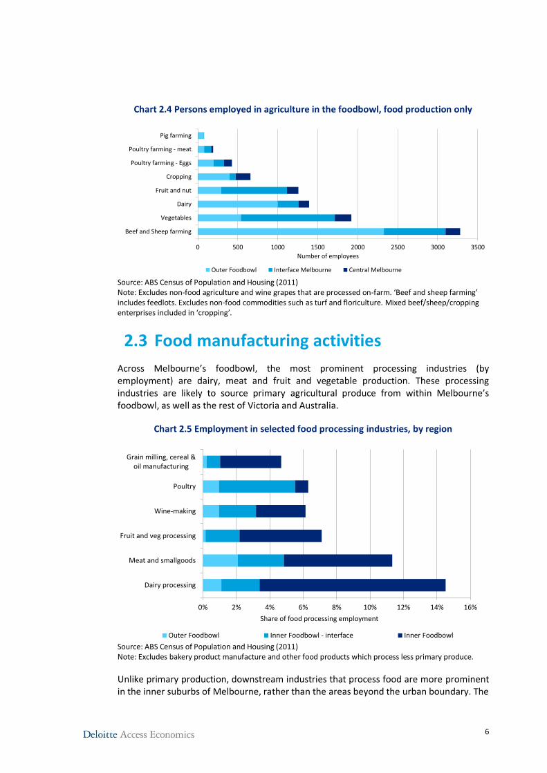
Chart 2.4 Persons employed in agriculture in the foodbowl, food production only

Source: ABS Census of Population and Housing (2011) Note: Excludes non-food agriculture and wine grapes that are processed on-farm. ‘Beef and sheep farming’ includes feedlots. Excludes non-food commodities such as turf and floriculture. Mixed beef/sheep/cropping enterprises included in ‘cropping’.

2.3 Food manufacturing activities

Across Melbourne’s foodbowl, the most prominent processing industries (by employment) are dairy, meat and fruit and vegetable production. These processing industries are likely to source primary agricultural produce from within Melbourne’s foodbowl, as well as the rest of Victoria and Australia.

Chart 2.5 Employment in selected food processing industries, by region

Source: ABS Census of Population and Housing (2011) Note: Excludes bakery product manufacture and other food products which process less primary produce.

Unlike primary production, downstream industries that process food are more prominent in the inner suburbs of Melbourne, rather than the areas beyond the urban boundary. The

0 500 1000 1500 2000 2500 3000 3500

Beef and Sheep farming

Vegetables

Dairy

Fruit and nut

Cropping

Poultry farming - Eggs

Poultry farming - meat

Pig farming

Number of employees

Outer Foodbowl Interface Melbourne Central Melbourne

0% 2% 4% 6% 8% 10% 12% 14% 16%

Dairy processing

Meat and smallgoods

Fruit and veg processing

Wine-making

Poultry

Grain milling, cereal &oil manufacturing

Share of food processing employment

Outer Foodbowl Inner Foodbowl - interface Inner Foodbowl

7

main exception to that is poultry, which tends to be processed close to where chickens are hatched and raised.5

The figures in the chart above include office-based employment in food processing industries. A number of food processing firms, such as dairy companies, have head-offices in Melbourne, which partially explains the relatively high proportion of employment in inner-areas. However, food processing plants are also located across inner Melbourne’s industrial areas.

The economic contribution of the foodbowl’s food processing sector, in terms of value added and employment, is discussed in Chapter 3.

2.4 Food consumption in Melbourne

There is no comprehensive data source on food consumption in Melbourne. Approaches to measuring food demand are therefore generated through multiplying population by an estimate of per-capita consumption for Australia.

Per-capita food consumption can either be estimated by using a national accounting approach (production less exports plus imports) or by using ABS nutritional data on the average intake across major food groups. In this report, the second approach has been used, following the same two-step approach adopted by the University of Melbourne’s Victorian Eco Innovation Lab in the Foodprint Melbourne project. The broad approach is to estimate the ‘average’ Australian diet by major food category using ABS nutritional data, which is survey-based, and applying that average intake to the population of Melbourne.

2.4.1 The ‘average’ Australian diet

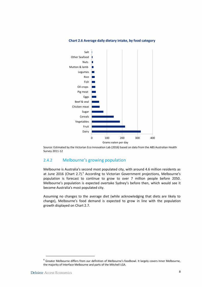
The average Australian diet, split into major food groups, is displayed in Chart 2.6 below. On average, Australians eat approximately 1.2 kilograms of food per day, consisting mostly of dairy, fruit, vegetables, grains and meat.

5 Australian Chicken Meat Federation: http://www.chicken.org.au/page.php?id=3

8

Chart 2.6 Average daily dietary intake, by food category

Source: Estimated by the Victorian Eco Innovation Lab (2016) based on data from the ABS Australian Health Survey 2011-12

2.4.2 Melbourne’s growing population

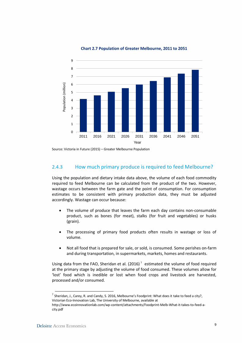
Melbourne is Australia’s second most populated city, with around 4.6 million residents as at June 2016 (Chart 2.7).6 According to Victorian Government projections, Melbourne’s population is forecast to continue to grow to over 7 million people before 2050. Melbourne’s population is expected overtake Sydney’s before then, which would see it become Australia’s most populated city.

Assuming no changes to the average diet (while acknowledging that diets are likely to change), Melbourne’s food demand is expected to grow in line with the population growth displayed on Chart 2.7.

6 Greater Melbourne differs from our definition of Melbourne’s foodbowl. It largely covers Inner Melbourne,

the majority of Interface Melbourne and parts of the Mitchell LGA.

0 100 200 300 400

Dairy

Fruit

Vegetables

Cereals

Sugar

Chicken meat

Beef & veal

Eggs

Pig meat

Oil crops

Fish

Rice

Legumes

Mutton & lamb

Nuts

Other Seafood

Salt

Grams eaten per day

9

Chart 2.7 Population of Greater Melbourne, 2011 to 2051

Source: Victoria in Future (2015) – Greater Melbourne Population

2.4.3 How much primary produce is required to feed Melbourne?

Using the population and dietary intake data above, the volume of each food commodity required to feed Melbourne can be calculated from the product of the two. However, wastage occurs between the farm gate and the point of consumption. For consumption estimates to be consistent with primary production data, they must be adjusted accordingly. Wastage can occur because:

The volume of produce that leaves the farm each day contains non-consumable product, such as bones (for meat), stalks (for fruit and vegetables) or husks (grain).

The processing of primary food products often results in wastage or loss of volume.

Not all food that is prepared for sale, or sold, is consumed. Some perishes on-farm and during transportation, in supermarkets, markets, homes and restaurants.

Using data from the FAO, Sheridan et al. (2016) 7 estimated the volume of food required at the primary stage by adjusting the volume of food consumed. These volumes allow for ‘lost’ food which is inedible or lost when food crops and livestock are harvested, processed and/or consumed.

7 Sheridan, J., Carey, R. and Candy, S. 2016, Melbourne’s Foodprint: What does it take to feed a city?, Victorian Eco-Innovation Lab, The University of Melbourne, available at http://www.ecoinnovationlab.com/wp-content/attachments/Foodprint-Melb-What-it-takes-to-feed-a-city.pdf

0

1

2

3

4

5

6

7

8

9

2011 2016 2021 2026 2031 2036 2041 2046 2051

Pop

ula

tio

n (m

illio

n)

Year

10

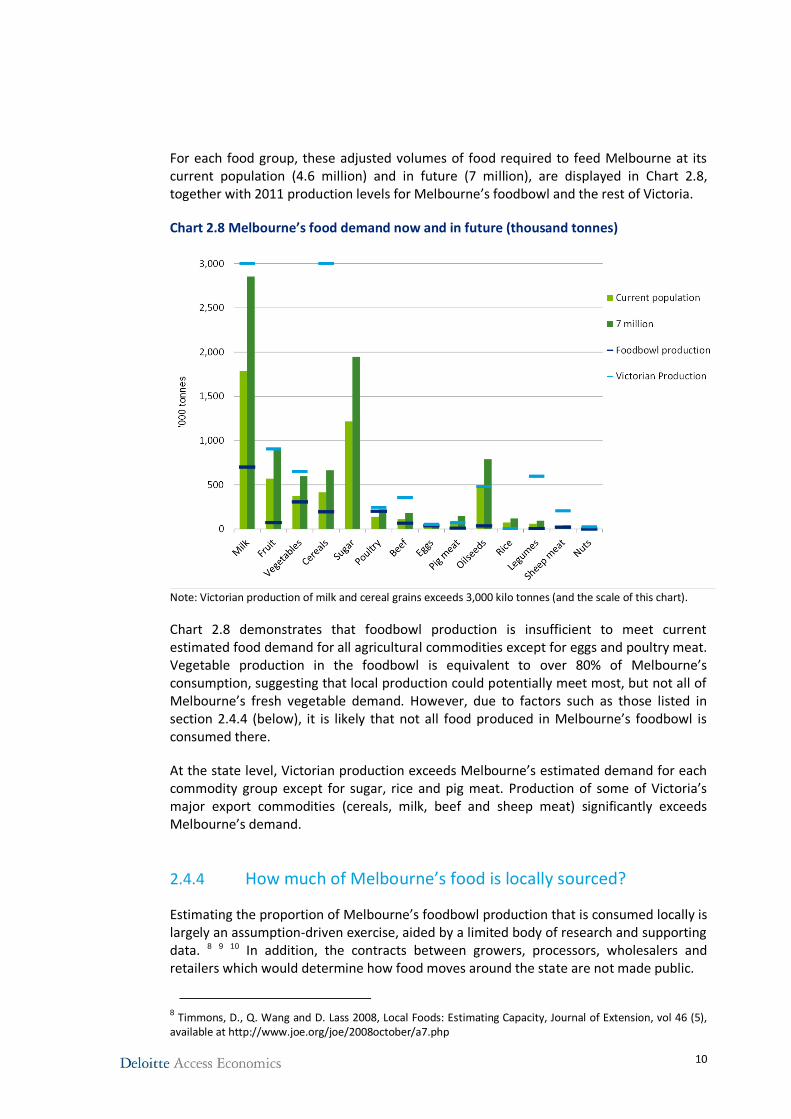
For each food group, these adjusted volumes of food required to feed Melbourne at its current population (4.6 million) and in future (7 million), are displayed in Chart 2.8, together with 2011 production levels for Melbourne’s foodbowl and the rest of Victoria.

Chart 2.8 Melbourne’s food demand now and in future (thousand tonnes)

Note: Victorian production of milk and cereal grains exceeds 3,000 kilo tonnes (and the scale of this chart).

Chart 2.8 demonstrates that foodbowl production is insufficient to meet current estimated food demand for all agricultural commodities except for eggs and poultry meat. Vegetable production in the foodbowl is equivalent to over 80% of Melbourne’s consumption, suggesting that local production could potentially meet most, but not all of Melbourne’s fresh vegetable demand. However, due to factors such as those listed in section 2.4.4 (below), it is likely that not all food produced in Melbourne’s foodbowl is consumed there.

At the state level, Victorian production exceeds Melbourne’s estimated demand for each commodity group except for sugar, rice and pig meat. Production of some of Victoria’s major export commodities (cereals, milk, beef and sheep meat) significantly exceeds Melbourne’s demand.

2.4.4 How much of Melbourne’s food is locally sourced?

Estimating the proportion of Melbourne’s foodbowl production that is consumed locally is largely an assumption-driven exercise, aided by a limited body of research and supporting data. 8 9 10 In addition, the contracts between growers, processors, wholesalers and retailers which would determine how food moves around the state are not made public.

8 Timmons, D., Q. Wang and D. Lass 2008, Local Foods: Estimating Capacity, Journal of Extension, vol 46 (5),

available at http://www.joe.org/joe/2008october/a7.php

11

While comparing likely local consumption with local agricultural production can demonstrate the likelihood that certain foods are sourced locally, there are other factors to consider, including:

• Perishability and freshness: Food that perishes easily is more likely to be locally sourced than that which can be stored for longer periods. For example, poultry meat has a relatively short shelf life (unless frozen), while rice and other grains can be stored for years without perishing.

• Seasonality: Where there is year-round demand, perishable fruit and vegetables that are in season for short windows must be sourced from elsewhere at various times throughout the year. Berries and capsicums are two examples – Victorian producers will send produce north when in season, while northern producers will meet Melbourne’s demand for part of the year. The share of locally sourced food consumed therefore varies throughout the year, which is not captured in annual production/consumption data.

• Definition of local: How businesses and consumers define ‘local’ can be subjective. For some, locally grown food can mean it was grown in the same country or the same state, while for others, the size of the radius which implies something is ‘local’ can be much smaller. Food produced in the foodbowl can enter bulk supply chains which span the state, other parts of the country, and can still be branded as ‘local’.

• Traceability: Even when local branding carries value, products that are highly commoditised are not easily traceable once pooled with produce from across the state and country. Cereal grains are one such example. This is in contrast with some horticulture, meat and eggs, where the origin can be easily communicated to consumers.

Applying these factors across a range of commodities, and informed by some consultation with industry, Deloitte Access Economics has developed a set of assumptions on how much of the foodbowl’s agricultural production is consumed locally. For the purpose of this analysis, local food is defined as food produced in Melbourne’s foodbowl that is consumed within the foodbowl region (which includes Greater Melbourne and outer foodbowl LGAs). These assumptions are outlined in Appendix C. While informed by data, these assumptions are only estimates to be used in the modelling that is discussed in Chapters 3 and 4.

9 Conner, D., F. Becot, D. Hoffer, E. Kahler, S. Sawyer and L. Berlin 2012, Measuring current consumption of locally grown foods in Vermont: Methods for baselines and targets, Journal of Agriculture, Food Systems and Community Development, available at http://mainefoodstrategy.com/wp-content/uploads/2013/05/jafscd_measuring_local_food_consumption_vermont_may-2013.pdf

10 Masi, B., L. Shaller and MH. Shuman 2010, The 25% shift: the benefits of food localization for Northeast Ohio

& how to realise them.

12

3 Economic contribution of Melbourne’s foodbowl

Deloitte Access Economics has estimated the economic contribution of Melbourne’s foodbowl. The estimation provides a snapshot of the economic footprint of agriculture and related value-adding activities in Melbourne’s foodbowl throughout the regional economy. This chapter describes the methodology and assumptions (section 3.1) and presents the results of the analysis (section 3.2).

3.1 Methodology

There are two parts to the economic contribution of Melbourne’s foodbowl; its direct contribution and its indirect contribution.

The direct contribution of an industry is measured as the value added by the activities of businesses within that industry, which is the sum of returns to labour and capital. Value added is a commonly adopted metric used to measure the economic contribution of industries and sub-sectors. This study measured the direct contribution of the agriculture and food manufacturing sectors in Melbourne’s foodbowl.

The indirect contribution of an industry is measured using Input-Output (IO) modelling. The linkages and interdependencies between various sectors of an economy are observed and used to analyse which outputs represent final demand and which flow to other sectors as inputs. The linkages between sectors are published by the ABS in the national accounts data.

Regional Input-Output model

Deloitte Access Economics has used the Global Trade Analysis Project (GTAP) input-output tables, which are based on the ABS national input-output tables, with the additional breakdown of agriculture into sub-sectors, including vegetable, poultry, and dairy production. Deloitte Access Economics then developed a regional-level IO model for Melbourne’s foodbowl with the following additional data:

• ABS 2011 census working population profile data (place of work) – used to infer regional production and consumption. In this case, agricultural production and consumption were inferred using sourcing assumptions outlined in appendix C.

• National import data - used to determine what is flowing into the region

• Trade flows between regions using local sourcing assumptions, which reflect that regional demand is met by local supply, distant supply and imports (see Section 2.4.4).

More details are provided in Appendix A.

13

3.2 Results

3.2.1 Economic contribution of agriculture and related value-adding activities in Melbourne’s foodbowl

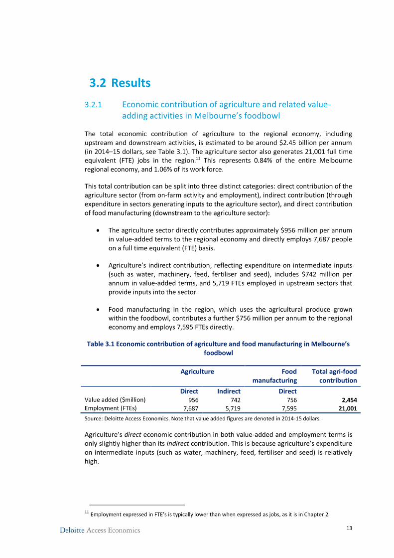
The total economic contribution of agriculture to the regional economy, including upstream and downstream activities, is estimated to be around $2.45 billion per annum (in 2014–15 dollars, see Table 3.1). The agriculture sector also generates 21,001 full time equivalent (FTE) jobs in the region.11 This represents 0.84% of the entire Melbourne regional economy, and 1.06% of its work force.

This total contribution can be split into three distinct categories: direct contribution of the agriculture sector (from on-farm activity and employment), indirect contribution (through expenditure in sectors generating inputs to the agriculture sector), and direct contribution of food manufacturing (downstream to the agriculture sector):

The agriculture sector directly contributes approximately $956 million per annum in value-added terms to the regional economy and directly employs 7,687 people on a full time equivalent (FTE) basis.

Agriculture’s indirect contribution, reflecting expenditure on intermediate inputs (such as water, machinery, feed, fertiliser and seed), includes $742 million per annum in value-added terms, and 5,719 FTEs employed in upstream sectors that provide inputs into the sector.

Food manufacturing in the region, which uses the agricultural produce grown within the foodbowl, contributes a further $756 million per annum to the regional economy and employs 7,595 FTEs directly.

Table 3.1 Economic contribution of agriculture and food manufacturing in Melbourne’s foodbowl

Agriculture

Food manufacturing

Total agri-food contribution

Direct Indirect Direct Value added ($million) 956 742 756 2,454 Employment (FTEs) 7,687 5,719 7,595 21,001

Source: Deloitte Access Economics. Note that value added figures are denoted in 2014-15 dollars.

Agriculture’s direct economic contribution in both value-added and employment terms is only slightly higher than its indirect contribution. This is because agriculture’s expenditure on intermediate inputs (such as water, machinery, feed, fertiliser and seed) is relatively high.

11

Employment expressed in FTE’s is typically lower than when expressed as jobs, as it is in Chapter 2.

14

3.2.2 Sectoral economic contribution

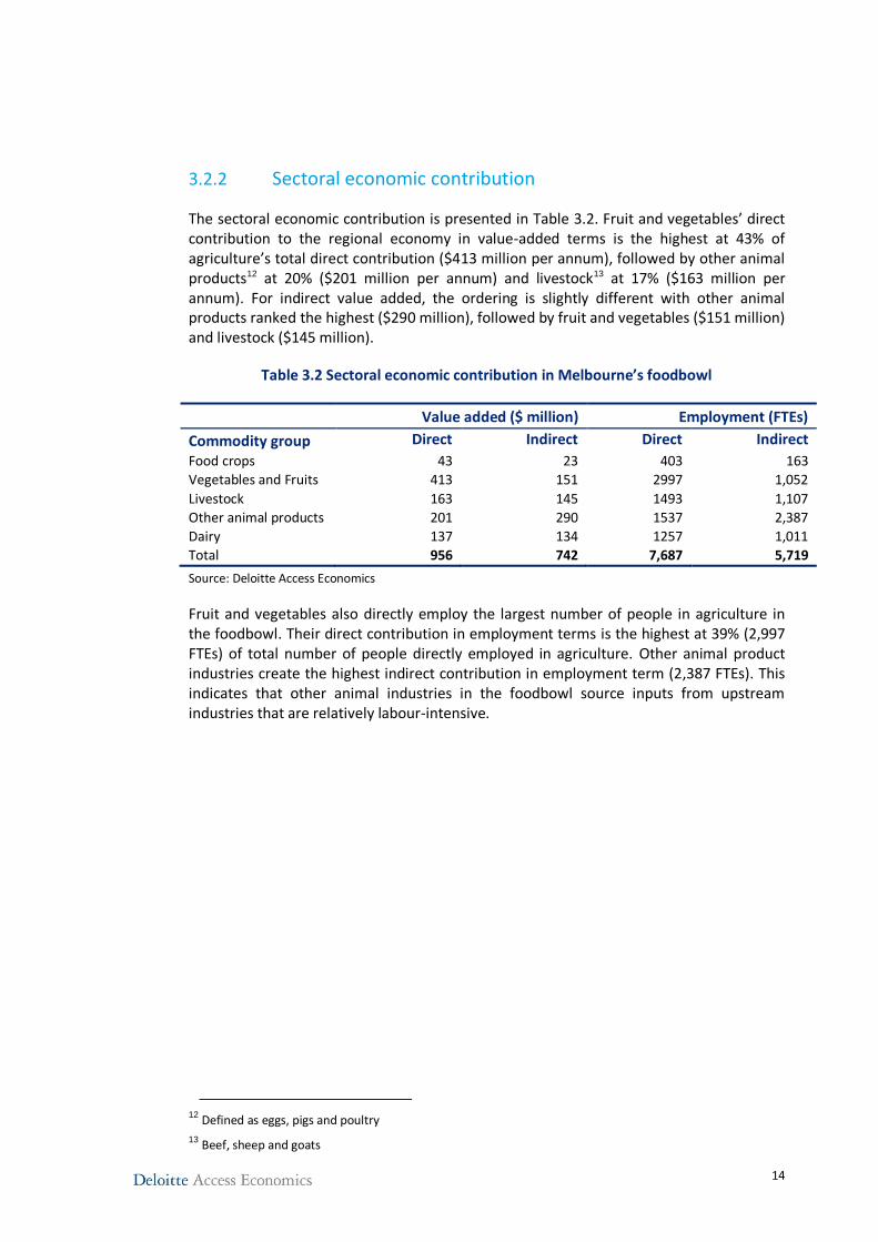
The sectoral economic contribution is presented in Table 3.2. Fruit and vegetables’ direct contribution to the regional economy in value-added terms is the highest at 43% of agriculture’s total direct contribution ($413 million per annum), followed by other animal products12 at 20% ($201 million per annum) and livestock13 at 17% ($163 million per annum). For indirect value added, the ordering is slightly different with other animal products ranked the highest ($290 million), followed by fruit and vegetables ($151 million) and livestock ($145 million).

Table 3.2 Sectoral economic contribution in Melbourne’s foodbowl

Value added ($ million) Employment (FTEs)

Commodity group Direct Indirect Direct Indirect

Food crops 43 23 403 163

Vegetables and Fruits 413 151 2997 1,052

Livestock 163 145 1493 1,107

Other animal products 201 290 1537 2,387

Dairy 137 134 1257 1,011

Total 956 742 7,687 5,719

Source: Deloitte Access Economics

Fruit and vegetables also directly employ the largest number of people in agriculture in the foodbowl. Their direct contribution in employment terms is the highest at 39% (2,997 FTEs) of total number of people directly employed in agriculture. Other animal product industries create the highest indirect contribution in employment term (2,387 FTEs). This indicates that other animal industries in the foodbowl source inputs from upstream industries that are relatively labour-intensive.

12 Defined as eggs, pigs and poultry

13 Beef, sheep and goats

15

4 Economic impacts under alternative future scenarios

In this chapter, the economic impacts of changes in land use from agricultural production to urban development to accommodate Melbourne’s 7 million people and changes in preference of consumers in Melbourne’s foodbowl for more locally grown food are estimated. This chapter describes the methodology and assumptions (section 4.1) and presents the results of the economic impact analysis under these changes (sections 4.2 and 4.3).

4.1 Methodology

This project utilises the Deloitte Access Economics – Regional General Equilibrium Model (DAE-RGEM). DAE-RGEM is a large scale, dynamic, multi-region, multi-commodity CGE model of the world economy that encompasses all economic activity in an economy – including production, consumption, employment, taxes and trade – and the linkages between them. For this project, the model has been customised to explicitly include Melbourne’s foodbowl regional economy and its unique economic characteristics.

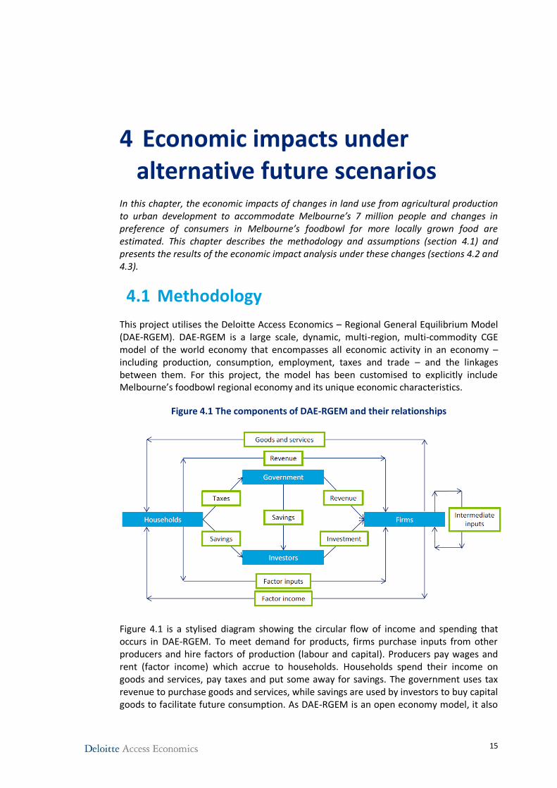
Figure 4.1 The components of DAE-RGEM and their relationships

Figure 4.1 is a stylised diagram showing the circular flow of income and spending that occurs in DAE-RGEM. To meet demand for products, firms purchase inputs from other producers and hire factors of production (labour and capital). Producers pay wages and rent (factor income) which accrue to households. Households spend their income on goods and services, pay taxes and put some away for savings. The government uses tax revenue to purchase goods and services, while savings are used by investors to buy capital goods to facilitate future consumption. As DAE-RGEM is an open economy model, it also

16

includes trade flows with other regions, states, and foreign countries. More details are provided in Appendix B.

Because Melbourne’s foodbowl is not explicitly represented in the database underlying DAE-RGEM, we customised the spatial regions of the model. Melbourne’s foodbowl consists of the Local Government Areas (LGAs) outlined in Table 2.1 and Figure 2.1.

In the following sections, the description of the scenarios and their results are discussed.

4.2 Melbourne growing to accommodate 7 million people

The study compares a baseline scenario of existing Melbourne land use to two alternative scenarios that reflect two alternative ‘sprawl’ scenarios where land currently used for agriculture is developed to accommodate a population of 7 million people, which is expected to occur between 2041 and 2046.14

The baseline scenario reflects the existing current land use profile of Melbourne’s foodbowl area. In order to isolate the effects of land use changes in each of the scenarios, population (which drives food demand) is held constant at 7 million people in the base case and the two scenarios.

The alternative scenarios, ‘constrained urban sprawl’ and ‘moderate urban sprawl’, reflect alternative ways in which Melbourne could grow to accommodate future population growth. The ‘constrained urban sprawl’ scenario represents a situation where less land is required for residential development than the ‘moderate urban sprawl’ scenario. The different rates of agricultural land retention reflect different assumptions about both the future density of existing residential areas (infill) and new housing developments. The assumptions driving each alternative scenario are summarised in Table 4.1.

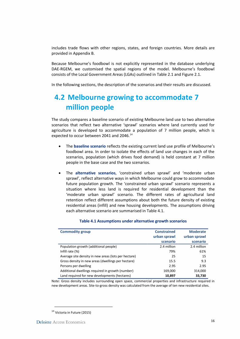
Table 4.1 Assumptions under alternative growth scenarios

Commodity group Constrained urban sprawl

scenario

Moderate urban sprawl

scenario Population growth (additional people) 2.4 million 2.4 million

Infill rate (%) 79% 61%

Average site density in new areas (lots per hectare) 25 15

Gross density in new areas (dwellings per hectare) 15.5 9.3

Persons per dwelling 2.95 2.95

Additional dwellings required in growth (number) 169,000 314,000

Land required for new developments (hectares) 10,897 33,730

Note: Gross density includes surrounding open space, commercial properties and infrastructure required in new development areas. Site-to-gross density was calculated from the average of ten new residential sites.

14

Victoria in Future (2015)

17

The assumptions presented in Table 4.1 have been informed by previous studies on Melbourne’s development. Buxton et al. (2015)15 estimated that an infill rate of around 79% could be achieved in Melbourne out to 2050. In other words, 79% of population growth could be accommodated by residential development within existing urban areas, with the remaining 21% developed in growth areas. It is worth noting that the infill rate of 79% is an aspirational goal. Plan Melbourne (2014) has a projected infill rate of 61%. These two alternative infill rates have been used in the ‘constrained urban sprawl’ and ‘moderate urban sprawl’ scenarios, respectively.

Assuming that dwellings in new developments will contain, on average, 2.95 people16, there will be 169,000 additional dwellings required in growth areas under the ‘constrained urban sprawl’ scenario and 314,000 additional dwellings required in growth areas under the ‘moderate urban sprawl’ scenario.

The average densities in the two scenarios are based on current guidelines for medium (25 per hectare) and low (15 per hectare) lot densities in new residential developments.17 Assuming (on average) high density developments, there will be approximately 11,000 hectares converted from agricultural land to residential land in the ‘constrained urban sprawl’ scenario. Assuming medium density development occurs, the equivalent area is around 34,000 hectares in ‘moderate urban sprawl’ scenario.

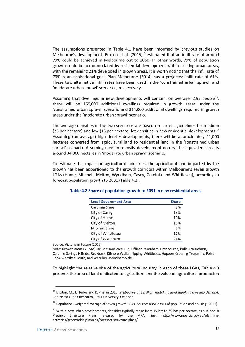
To estimate the impact on agricultural industries, the agricultural land impacted by the growth has been apportioned to the growth corridors within Melbourne’s seven growth LGAs (Hume, Mitchell, Melton, Wyndham, Casey, Cardinia and Whittlesea), according to forecast population growth to 2031 (Table 4.2).

Table 4.2 Share of population growth to 2031 in new residential areas

Local Government Area Share

Cardinia Shire 9%

City of Casey 18%

City of Hume 10%

City of Melton 16%

Mitchell Shire 6%

City of Whittlesea 17%

City of Wyndham 24%

Source: Victoria in Future (2015) Note: Growth areas (VIFSAs) include: Koo Wee Rup, Officer-Pakenham, Cranbourne, Bulla-Craigieburn, Caroline Springs-Hillside, Rockbank, Kilmore-Wallan, Epping-Whittlesea, Hoppers Crossing-Truganina, Point Cook-Werribee South, and Werribee-Wyndham Vale.

To highlight the relative size of the agriculture industry in each of these LGAs, Table 4.3 presents the area of land dedicated to agriculture and the value of agricultural production

15

Buxton, M., J. Hurley and K. Phelan 2015, Melbourne at 8 million: matching land supply to dwelling demand, Centre for Urban Research, RMIT University, October.

16 Population–weighted average of seven growth LGAs. Source: ABS Census of population and housing (2011)

17 Within new urban developments, densities typically range from 15 lots to 25 lots per hectare, as outlined in Precinct Structure Plans released by the MPA. See: http://www.mpa.vic.gov.au/planning-activities/greenfields-planning/precinct-structure-plans/

18

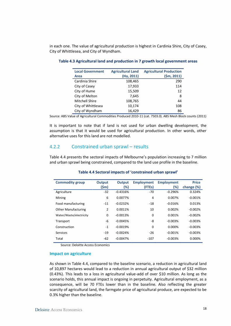
in each one. The value of agricultural production is highest in Cardinia Shire, City of Casey, City of Whittlesea, and City of Wyndham.

Table 4.3 Agricultural land and production in 7 growth local government areas

Local Government Area

Agricultural Land (Ha, 2011)

Agricultural Production ($m, 2011)

Cardinia Shire 108,465 290

City of Casey 17,933 114

City of Hume 15,509 12

City of Melton 7,645 8

Mitchell Shire 108,765 44

City of Whittlesea 10,174 108

City of Wyndham 16,429 86

Source: ABS Value of Agricultural Commodities Produced 2010-11 (cat. 7503.0). ABS Mesh Block counts (2011)

It is important to note that if land is not used for urban dwelling development, the assumption is that it would be used for agricultural production. In other words, other alternative uses for this land are not modelled.

4.2.2 Constrained urban sprawl – results

Table 4.4 presents the sectoral impacts of Melbourne’s population increasing to 7 million and urban sprawl being constrained, compared to the land use profile in the baseline.

Table 4.4 Sectoral impacts of ‘constrained urban sprawl’

Commodity group Output ($m)

Output (%)

Employment (FTEs)

Employment (%)

Price change (%)

Agriculture -32 -0.4316% -70 -0.296% 0.324%

Mining 6 0.0077% 4 0.007% -0.001%

Food manufacturing -11 -0.0232% -18 -0.016% 0.013%

Other Manufacturing 2 0.0011% 10 0.002% -0.002%

Water/Waste/electricity 0 -0.0013% 0 0.001% -0.002%

Transport -6 -0.0045% -8 -0.003% -0.003%

Construction -1 -0.0019% 0 0.000% -0.003%

Services -19 -0.0024% -26 -0.001% -0.003%

Total -62 -0.0047% -107 -0.003% 0.000%

Source: Deloitte Access Economics

Impact on agriculture

As shown in Table 4.4, compared to the baseline scenario, a reduction in agricultural land of 10,897 hectares would lead to a reduction in annual agricultural output of $32 million (0.43%). This leads to a loss in agricultural value-add of over $10 million. As long as the scenario holds, this annual impact is ongoing in perpetuity. Agricultural employment, as a consequence, will be 70 FTEs lower than in the baseline. Also reflecting the greater scarcity of agricultural land, the farmgate price of agricultural produce, are expected to be 0.3% higher than the baseline.

19

Impact on food manufacturing and the regional economy

Food manufacturing is a downstream sector of agricultural production. As a result of declining agricultural output, food manufacturing’s annual output will decrease by $11 million (0.023%) under the constrained urban sprawl scenario, relative to the baseline scenario. As previously discussed, as long as the scenario holds, this impact on food manufacturing’s output is ongoing in perpetuity.

Reflecting a lower level of output in food manufacturing, employment in this sector in Melbourne’s foodbowl will decrease by 18 FTEs compared to the baseline scenario. Compared to the 7,595 FTEs directly employed in food manufacturing in Melbourne’s foodbowl, this amount appears modest, however the impact could be concentrated to particular areas depending on the agricultural land affected.

Similarly, the price of processed foods is expected to increase under the scenario, reflecting a reduction in Melbourne’s food supply. It is estimated that prices of these products will be 0.013% higher than the baseline (Table 4.4).

As a result of declining agricultural output, there are other flow-on effects to the rest of the economy (see Table 4.4). In particular, the economy’s annual output falls by $62 million (0.0047%), leading to a reduction in the GRP of Melbourne’s foodbowl of $35 million and a decrease in regional employment of 107 FTEs, relative to the baseline scenario.

Overall, the annual impacts on the regional economy appear to be modest. However, the cumulative impacts of this scenario could be significant. As long as the same impacts on gross regional product18 (GRP) occur every year from, for example, 2050 to 2070, the net present value of the cumulative impact would be $376 million (in 2014–15 dollars). It is noted this estimate represents a best case scenario, because as population continues to grow, urban development will also continue.

4.2.3 Moderate urban sprawl – results

Table 4.5 presents the sectoral and price impacts of Melbourne’s population increasing to 7 million and urban sprawl occurring at a faster rate under the second of the two alternative scenarios.

Impact on agriculture

The impact of the ’moderate urban sprawl’ scenario would lead to a reduction of annual agricultural production of $111 million (1.49%), relative to the baseline scenario. This leads to a loss in agricultural value-add of around $35 million. Agricultural employment will be 240 FTEs lower. The reason that the economic impacts on agriculture would be higher in this scenario than in the ‘constrained urban sprawl’ scenario is that less constrained urban sprawl would lead to more agricultural land loss, hence, a bigger loss to agricultural output.

18

Gross regional product refers to the annual output of a regional economy, just as gross domestic product (GDP) refers to the annual output of a national economy

20

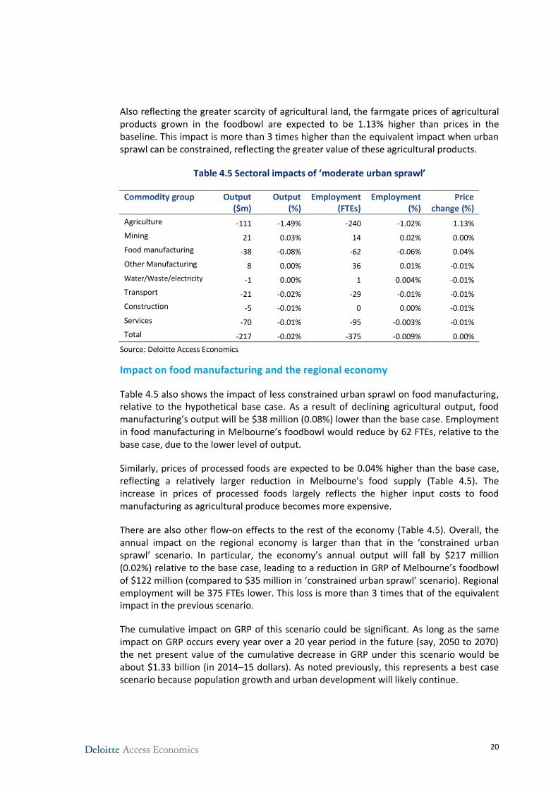
Also reflecting the greater scarcity of agricultural land, the farmgate prices of agricultural products grown in the foodbowl are expected to be 1.13% higher than prices in the baseline. This impact is more than 3 times higher than the equivalent impact when urban sprawl can be constrained, reflecting the greater value of these agricultural products.

Table 4.5 Sectoral impacts of ‘moderate urban sprawl’

Commodity group Output ($m)

Output (%)

Employment (FTEs)

Employment (%)

Price change (%)

Agriculture -111 -1.49% -240 -1.02% 1.13%

Mining 21 0.03% 14 0.02% 0.00%

Food manufacturing -38 -0.08% -62 -0.06% 0.04%

Other Manufacturing 8 0.00% 36 0.01% -0.01%

Water/Waste/electricity -1 0.00% 1 0.004% -0.01%

Transport -21 -0.02% -29 -0.01% -0.01%

Construction -5 -0.01% 0 0.00% -0.01%

Services -70 -0.01% -95 -0.003% -0.01%

Total -217 -0.02% -375 -0.009% 0.00%

Source: Deloitte Access Economics

Impact on food manufacturing and the regional economy

Table 4.5 also shows the impact of less constrained urban sprawl on food manufacturing, relative to the hypothetical base case. As a result of declining agricultural output, food manufacturing’s output will be $38 million (0.08%) lower than the base case. Employment in food manufacturing in Melbourne’s foodbowl would reduce by 62 FTEs, relative to the base case, due to the lower level of output.

Similarly, prices of processed foods are expected to be 0.04% higher than the base case, reflecting a relatively larger reduction in Melbourne’s food supply (Table 4.5). The increase in prices of processed foods largely reflects the higher input costs to food manufacturing as agricultural produce becomes more expensive.

There are also other flow-on effects to the rest of the economy (Table 4.5). Overall, the annual impact on the regional economy is larger than that in the ‘constrained urban sprawl’ scenario. In particular, the economy’s annual output will fall by $217 million (0.02%) relative to the base case, leading to a reduction in GRP of Melbourne’s foodbowl of $122 million (compared to $35 million in ‘constrained urban sprawl’ scenario). Regional employment will be 375 FTEs lower. This loss is more than 3 times that of the equivalent impact in the previous scenario.

The cumulative impact on GRP of this scenario could be significant. As long as the same impact on GRP occurs every year over a 20 year period in the future (say, 2050 to 2070) the net present value of the cumulative decrease in GRP under this scenario would be about $1.33 billion (in 2014–15 dollars). As noted previously, this represents a best case scenario because population growth and urban development will likely continue.

21

4.2.4 Discussion

The result from the two urban sprawl scenarios highlights how accommodating Melbourne’s growing population will result in a loss of agricultural land at varying degrees, reducing output and employment in both the agricultural and food manufacturing industries. Comparing the results of the two scenarios shows how the negative economic impacts on GRP and employment, could be minimised by constraining urban sprawl, primarily through retaining agricultural land. If population is growing according to current trends, expanding urban sprawl would lead to significant negative impacts on these measures in the future.

At the sectoral level, the negative impacts on agriculture and food manufacturing are the result of the loss in agricultural land, hence, agricultural output. Lower food supply resulting from less available agricultural land would likely lead to higher farmgate prices for primary produce, and higher prices for processed foods. These price increases would be expected to be passed through the supply chain, resulting in higher retail food prices for consumers, although the prices impact will be small since the farmgate or wholesale price (at factory door) represents only a small share of the price paid by consumers.

These results show that negative impacts on agriculture seem to be minimised by constraining urban sprawl. Relative to the base case, annual agricultural output falls by $32 million (over $10 million in value-add) while employment falls by 70 FTEs (full time equivalents) under the ‘constrained urban sprawl’ scenario. Under the ‘moderate urban sprawl’ scenario, agricultural production falls by $111 million (around $35 million in value-add) while agricultural employment falls by 217 FTEs.

As a result of declining agricultural output, there are other negative flow-on effects for the rest of the economy in the foodbowl area, particularly in the food manufacturing sector. These flow-on effects are larger in the ‘moderate urban sprawl’ scenario. Relative to the baseline, the economy’s annual output will be $62 million lower under the ‘constrained urban sprawl’ scenario and $217 million lower under the ‘moderate urban sprawl’ scenario.

In the context of other pressures, such as climate change, declining supplies of other natural resources (particularly water) and pressures on the fresh food supply from other peri-urban areas around Australian capital cities, this loss of agricultural land and reduction in output presents a risk to Melbourne’s food security. Some of Melbourne’s fastest growing residential areas are encroaching on agricultural areas with access to water supplies that are largely rainfall independent, particularly recycled water from Melbourne’s two large water treatment plants. The impact on Melbourne’s food supply would be particularly acute during drought years, and over time as Melbourne’s population grows larger. These issues are discussed in greater detail in Chapter 5.

22

4.3 Increasing preference for ‘local’ food

The analysis also examines the economic impact of an increased preference for local food. It compares the baseline scenario which reflects current preferences for locally-sourced food19 with an alternative scenario, where preferences for local food increase by 10% for most food products20.

In the baseline, a set of assumptions surrounding local sourcing were developed (see Appendix C). For highly perishable food products such as fruits and vegetables, chicken meat, eggs and pig meat, the share of foodbowl production consumed by residents living within Melbourne’s foodbowl is medium to high. For other products, where there is less of a preference for local sourcing, the amount that is consumed locally is relatively low.

In the alternative scenario, the quantity of produce that is grown and consumed within the Melbourne foodbowl is assumed to increase by 10% for most commodities. This scenario excludes cereals, oil seeds and legumes – commoditised crops which are usually highly processed and therefore less traceable at the point of consumption. It is assumed in the alternative scenario that there would be capacity to increase agricultural output in the foodbowl to meet the increase in demand for local food by increasing the intensity of production on existing agricultural land. This also assumes access to the inputs and infrastructure required to increase the intensity of production, particularly access to sufficient water.

4.3.1 Results

This section presents the economic impacts of the shift in preference of residents of Melbourne’s foodbowl for more ‘locally-grown’ food, relative to the baseline described above. The preference shift would be expected to generate a supply response, increasing annual agricultural output by $290 million (7.41%) compared to the base case. This leads to an increase in agricultural value-add of around $131 million.

Agricultural employment would be 1,183 FTEs higher than the baseline if local food consumption was increased by 10% for most agricultural products. This increase is significant when compared to the 7,687 FTEs directly employed in the sector.

Under this alternative scenario, the farmgate prices of agricultural production within Melbourne’s foodbowl will increase by 5.29%, reflecting the higher local demand for food products grown there. This price increase, however, only relates to produce grown within Melbourne’s foodbowl. The preference shift will have negligible impact on the price of agricultural commodities grown across other parts of the country and internationally. The price impact to Melbourne’s consumers, therefore, is expected to be significantly less than this, since for most food commodities, a significant share of food consumed in Melbourne is grown outside of the foodbowl.

19 For residents living in the food bowl, includes those in Outer Foodbowl areas, such as Geelong and Warragul.

20 Excludes cereal grains and oilseeds

23

Additionally, the price paid to agricultural producers represents a fraction of the price paid by consumers, with the balance made up by other points along the value chain, such as processing, wholesale mark-up, retail mark-up and transport. For some processed livestock products, this share can be as little as 10% of the retail price paid by consumers21. Therefore, the increase to the price paid by consumers will be dampened, assuming that other costs remain relatively constant.

4.3.2 Discussion

An increase in preference for locally grown produce from Melbourne residents would likely result in greater value being placed on food grown within the foodbowl area. As the price increases, producers within Melbourne’s foodbowl would respond by increasing agricultural output, which would also result in an increase in the number of jobs in the agriculture sector.

The flow-on effects of this scenario to the rest of the economy are mixed, with a positive outcome for some sectors and negative for some others. As a downstream sector of agriculture, when agricultural output increases, food manufacturing would be expected to increase as well. However, locally-grown agricultural products are an input into Melbourne’s food manufacturing sector. The higher prices for this particular input will lead to a slight decrease in output from the sector. However, as local agricultural produce is only one of many inputs, including produce from other parts of Victoria and Australia, the impact of higher agricultural prices on food manufacturing is expected to be relatively small. Resources are expected to be reallocated from other sectors in the economy to service the increase in agricultural output, which partly explains the mixed outcomes in the rest of the economy.

These results highlight how such a shift would increase the prices offered to agricultural producers in the foodbowl area, and encourage land owners to maximise agricultural output. If such a shift were to be ongoing, it would lead to greater resilience of Melbourne’s local food supply, among other ancillary benefits which will be discussed in Chapter 5.

21

ACCC (2008), Report of the ACCC inquiry into the competitiveness of retail prices for standard groceries, Australian Competition and Consumer Commission, Canberra, July.

24

5 Ancillary benefits This chapter provides information on potential ancillary benefits of food production (and related value-adding activities) in Melbourne’s foodbowl. These are benefits not captured in the economic contribution and economic impact analysis of the above chapters.

5.1 Insurance and option value

Keeping land in agricultural production in Melbourne’s foodbowl may provide insurance against a number of risks.

Firstly, it would provide the insurance value against drought and climate change that can come through rainfall independent sources of food production when treated recycled waste water from Melbourne is used for food production in the foodbowl. Parts of the foodbowl that are in close proximity to highly secure water sources – the Eastern and Western Treatment Plants–have access to recycled water to produce vegetables during drought.22 23 There are also schemes using recycled water for agriculture near some of the smaller water treatment plants around Melbourne, such as the Boneo Treatment Plant in the South-East.

According to Sheridan et al. (2016), 10% of the available recycled water would be enough to grow half of the vegetables that Melbourne eats, 15% would double the amount of water needed to produce all of lamb eaten by Melbourne and 20% would be enough to produce 70% of the nuts eaten by Melbourne.24 As climate change will impact food production through water scarcity, the proximity to these secure water resources enables Melbourne’s foodbowl to contribute to the resilience of the food supply.

Secondly, removing land in the foodbowl from food production would, all else being equal, result in reduced geographical diversification of the food production system, and reduced resilience of the food supply. This would make the system as a whole – including the price and availability of food – more exposed to the seasonal conditions experienced in the remaining food production areas that Melbourne relies on. In addition, not retaining some local sources of food production would lead to greater dependence on distant sources of food and more exposure to potential shocks from extreme weather events (such as droughts, floods and bushfires).

Thirdly, retaining land in agricultural production in Melbourne’s foodbowl may provide insurance against biosecurity risks. Australia’s food standards system is one of the best in the world. As a result, we have relatively few food safety incidents. If land within Melbourne’s foodbowl is transitioned from agricultural use, which in turns lead

22 Carey, R., Larsen, K. and Sheridan, J. (2015), The role of cities in climate resilient food systems: A Foodprint Melbourne briefing, Victorian Eco-Innovation Lab, The University of Melbourne.

23 Sheridan, J., Carey, R. and Candy, S. (2016), Melbourne’s Foodprint: What does it take to feed a city? Victorian Eco-Innovation Lab, The University of Melbourne.

24 Ibid.

25

Melbournians to source food from other jurisdictions, subject to different food standards, the likelihood of food safety incidents could increase. To an extent, the quality and safety of food from different sources can be captured in market prices, but it is precisely those risks that cannot be observed and priced that Australian food safety regimes aim to mitigate.

Land which is retained in agriculture gives society the option value for future land use. Based on the observed development patterns, it is highly unlikely that once land has been developed, particularly for residential uses, it will rarely be returned to farmland or open space. While it could be argued that there is nothing necessarily preventing returning land from, for example, urban residential uses to agricultural use, there are a range of zoning and buffer zone regulations that would in practice make it very costly to create new agricultural land in the midst of an urban area.

5.2 Visual amenity

A range of potential benefits from preserving land for agricultural use have long been recognised in the economics literature. A useful taxonomy introduced in 1977 identified four distinct categories of benefits:

sufficient food and fibre to meet population needs;

local economic benefits from a viable agricultural industry;

more efficient and orderly suburban development; and

open space and other environmental amenities.25

The first of these is likely to occur–market forces will lead to an allocation of resources that provides for sufficient quantities of food and fibre products. However, it is worth noting that relying on market forces alone might not be sufficient when there are market failures resulting from issues such as climate change and extreme weather events. In the presence of market failures, the role of planning for food production in the future will become necessary. The second has been quantitatively estimated in the above chapters in the form of economic contribution and impact analysis. The third relates to whether zoning decisions that give precedence to agriculture will have desirable efficiency or equity properties, and is in a sense beyond the scope of the current analysis.

The final category – open space and environmental amenities – falls directly within the purview of this chapter.

The value of open space has been explicitly recognised in Victorian planning since at least 1971:

Land use, resources, terrain, vegetation and habitat vary extensively throughout the non-urban areas. It is intended that the basic attributes and resources contained within the areas shall be preserved to a maximum

25

Gardner, B. (1977), The economics of agricultural land preservation, American Journal of Agricultural Economics, Vol. 59 No. 5 pp1027-1036.

26

degree, and that environment management policies shall be specifically oriented towards this objective.26

Today, the broader benefits of land used for agriculture or other low-density activities is recognised in the fact that there are 12 designated Green Wedge areas in Victoria, spread across 17 municipalities surrounding Melbourne.27 There is a significant overlap between these Green Wedges and Melbourne’s foodbowl.

The benefits that these open spaces can provide are recognised in Green Wedge Management Plans. For example, it is one of the explicit objectives of the Whittlesea Green Wedge Management Plan 2011-2021: “to conserve and enhance the rural and natural landscape character of the Whittlesea Green Wedge”. A common message regarding this objective was distilled from consultation that fed into the Management Plan:

Our rural landscape is a highly valued feature of the green wedge and should be protected from urban development and infrastructure.28

While it is not possible to quantify the value of these benefits to residents of Melbourne’s foodbowl or how they would vary under a counterfactual scenario, being able to do so would count positively towards retaining land in Green Wedges in current uses, including agricultural use.

5.3 Other ancillary benefits

The most obvious area in which the local supply of food may economise on environmental impacts is through the carbon footprint associated with transporting goods from farms to processing facilities, and on to distribution facilities. The following discussion will show that it is not possible to draw clear conclusions about the value of local food consumption for energy use and emissions reduction.

The GHG emissions associated with transport of raw and processed food products could be classified as Scope 3 emissions – emissions that are not directly associated with the production process (Scope 1 emissions), or the generation of electricity (Scope 2 emissions), but are generated as part of the supply chain.

If Melbourne’s residents sourced food products from other parts of Australia, this would likely entail greater carbon emissions. Without any further information, it is reasonable to assume that different food producers across Australia have similar Scope 1 and Scope 2 emissions per unit of food produced. That is, their production technologies and their sources of electricity are relatively similar. They would, however, differ in the distances that food would need to be transported to be consumed in Melbourne (Scope 3 emissions), with food produced elsewhere needing to be transported further. Indeed, GHG emissions associated with the transport of fruit and vegetables transported to

26 Melbourne and Metropolitan Board of Works (1971), Planning Policies for Metropolitan Melbourne.

27 Department of Transport, Planning and Local Infrastructure Victoria (2016), Green Wedges. URL http://www.dtpli.vic.gov.au/planning/plans-and-policies/green-wedges, accessed 30 May 2016.

28 City of Whittlesea (2011), Whittlesea Green Wedge Management Plan 2011-21.

27

Victoria from other Australian jurisdictions could be around four times those from produce sourced from within Victoria.29

If products were instead sourced internationally rather than being produced locally, Scope 1 and 2 emissions would likely become relatively more important. Research undertaken for the Victorian Eco-Innovation Lab found that transport emissions associated with internationally sourced fruit and vegetables would actually be similar to those for produce sourced from other Australian jurisdictions (though this analysis did not account for in-country movement of fruit and vegetables produced in other countries).30

While Australian agriculture is among the most emissions-intensive in the world31, it is not possible to know at this stage whether producing food in Melbourne’s foodbowl or where it might otherwise be produced internationally would entail more or less Scope 1 and 2 emissions in total.32

Given the range of factors that need to be considered in an analysis of this type, it is not surprising that there is no clear and necessary conclusion that can be drawn about the benefits of energy use and emissions reduction by local food production.33

A complete analysis of the relative environmental impacts of having food consumed in Melbourne produced in its foodbowl or elsewhere would require clear articulation of a reasonable counterfactual scenario. This would define where Melbournians would otherwise source food from, and calculation of Scope 1, 2 and 3 emissions associated with each supply chain.

5.4 Future ancillary benefits

Ancillary benefits of Melbourne’s foodbowl are likely to increase as the population grows. This is straightforward. The benefits discussed above are predicated on the idea that people value green and open spaces – additional people increases the total potential value that these spaces can provide.

It also possible that future Greater Melbourne’s residents would value agricultural land for the environmental and amenity benefits to a greater extent than residents today. Population growth that is geographically constrained (as future population is likely to be,

29 Marquez, L., Higgins, A. and Estrada-Flores, S. (2010), Understanding Victoria’s Fruit and Vegetable Freight Movements. Report for the Victorian Eco-Innovation Lab.

30 Marquez, L., Higgins, A. and Estrada-Flores, S. (2010), Understanding Victoria’s Fruit and Vegetable Freight Movements. Report for the Victorian Eco-Innovation Lab.

31 Garnaut, R. (2011), The Garnaut Review 2011: Australia in the Global Response to Climate Change, available at http://www.garnautreview.org.au/update-2011/garnaut-review-2011/summary-20June.pdf.

32 Note while it is likely not feasible for a number of highly perishable products to be imported, if they were, they would need to be transported via air freight, which would almost certainly entail a net increase in emissions associated with transport.

33 Martinez, S., Hand, M., Da Pra, M., Pollack, S., Ralston, K., Smith, T., Vogel, S., Clark, S., Lohr, L., Low, S. and Newman, C. (2010), Local Food Systems: Concepts, Impacts, and Issues. United States Department of Agriculture Economic Research Service, Economic Research Report Number 97.

28

to some extent) could result in even greater contrasts between the amenity values of urban and rural areas, which may increase the value put on farmland.34

A nascent area of activity that could increase the economic contribution of Melbourne’s foodbowl as an area dominated by farms and open spaces is agri-tourism. The value of farm tourism accommodation was estimated to be around $115 million in 2006 (less than half of one per cent of the value of agricultural commodities produced in that year).35 A 2010 study found that there are already a number of farm businesses active in the tourism space in East Gippsland, with horticulture-related farms dominating.36 While some farms were able to generate a large share of their income from tourism-related activities, a need to acquire new skills of being a tourism operator and potentially significant capital outlays are barriers to involvement in the sector.

5.5 Note on ancillary benefits

This chapter has discussed a number of the potential benefits of land being used for agriculture. The discussion does not, however, constitute an evaluation of alternative land use scenarios.

A complete comparative analysis of alternative land use scenarios would require quantification of, at least, the potential benefits discussed above, as well as potential costs. Agriculture can impose negative externalities on nearby residents (for example, runoffs, odour, noise and dust have been identified as negative externalities of the broiler industry).37

A complete comparative analysis would also need to compare the non-market benefits and costs against the financial benefits and costs of alternative land use options. The relative willingness to pay for residential land and farmland would have an important role in such analysis.

34

Kline, J. and Wilchens, D. (1996), Public preferences regarding the goals of farmland preservation programs, Land Economics, Vol. 72, pp538-549; Nickerson, C.J. and Hellerstein, D. (2003), Protecting rural amenities through farmland preservation programs, Agricultural and Resource Economics Review, Vol. 32, pp129-144.

35 Ollenburg, C. (2006), Farm Tourism in Australia: A Family Business and Rural Studies Perspective, PhD thesis, School of Environmental and Applied Sciences, Faculty of Environmental Sciences, Griffith University.

36 Ecker, S., Clarke, R., Cartwright, S., Kancans, R., Please, P. and Binks, B. (2010), Drivers of regional agritourism and food tourism in Australia. Australian Bureau of Agricultural and Resource Economics – Bureau of Rural Sciences report.

37 Henderson, S. and Epps, R. (2000), Urban Fringe Land Use Conflict: Two Case Studies, A report for the Rural Industries Research and Development Corporation, Human and Environmental Studies, University of New England, Armidale.

29

6 Conclusion Economic contribution of agriculture to Melbourne’s foodbowl

The economic contribution of Melbourne’s foodbowl has been modelled by Deloitte Access Economics.

Agriculture directly contributes approximately $956 million per annum in value-added terms to the regional economy and employs 7,687 people on a FTE basis.

The sector also generates upstream and downstream activity in other sectors:

Agriculture’s expenditure on inputs generated $742 million per annum in value-added terms, and creates 5,719 FTEs in those upstream sectors that provide inputs into the sector.

Food manufacturing in the region, attributable to agriculture grown in the foodbowl area, contributes a further $756 million per annum to the regional economy and employs an annual total of 7,595 FTEs directly.

Summing these three categories, the total economic contribution of agriculture, including upstream and downstream activities, to the Melbourne’s foodbowl economy is $2.45 billion and 21,001 FTE jobs. These figures represent 0.84% of the foodbowl’s total economic activity, and 1.06% of its work force.

Economic impacts of urban sprawl

Deloitte Access Economics also modelled the economic impacts of changes in land use and changes in consumer preference that would impact on agriculture, food manufacturing and the regional economy as a whole.

The first of these changes was the impact that urban sprawl will have on Melbourne’s foodbowl and regional economy. The study examined two alternative ‘urban sprawl’ scenarios where land currently used for agriculture is developed to accommodate a population of 7 million people. One of the alternative scenarios modelled was a ‘constrained urban sprawl’ scenario, where the food producing area in the foodbowl is reduced by 10,897 ha, or 0.62%. The other was a moderate sprawl scenario, where the food producing area is reduced by 33,730 ha, or 1.92%. These alternative scenarios were modelled and compared with the current agricultural land use profile of Melbourne’s foodbowl.

The modelling results showed that urban sprawl would lead to significant loss to the regional economy. The economy’s annual output will be $62 million lower under the ‘constrained urban sprawl’ scenario and $217 million lower under the ‘moderate urban sprawl’ scenario. The loss to regional employment will be three times higher in the

30

‘moderate urban sprawl’ scenario than in the ‘constrained urban sprawl’ scenario (375 FTEs compared to 107 FTEs)

For agriculture, annual agricultural output would fall under both of these alternative scenarios, but the extent of the decrease was significantly larger in the scenario where urban sprawl was not constrained. The modelling results demonstrate that constraining urban sprawl could limit the loss to agricultural output and employment in the sector and the flow-on effects to the rest of the economy. Furthermore, constraining urban sprawl would limit the impact that a fall in supply would have on farmgate prices.

Reducing agricultural land to accommodate for population growth poses a risk to the foodbowl in terms of potential loss to agricultural output and rising food prices, adding to other pressures on food prices from climate change, declining supplies of other natural resources (particularly water) and pressures on fresh food supply from other peri-urban foodbowls around Australian capital cities.

Economic impacts of preferring ‘local’ food

The second of these changes was a scenario in which a shift in consumers’ preferences in Melbourne’s foodbowl results in an increase in the consumption local food. The results demonstrated that such a preference shift would stimulate agricultural production in the foodbowl area, which would lead to potentially higher agricultural output and employment. Overall, this would have mixed outcomes in the rest of economy as resources are reallocated from other sectors towards agriculture and related industries.

Ancillary benefits of food production in Melbourne’s foodbowl

There are also ancillary benefits of retaining land in Melbourne’s foodbowl, particularly on the peri-urban fringe, for agricultural production. These benefits, which are not captured in the modelling, include:

the insurance value against drought and climate change;

the option value of land use that is retained in farming but lost once land is developed;

enhanced visual amenity; and

other ancillary benefits.

It is worth noting, however, that our discussion in this study does not constitute an evaluation of alternative land use scenarios.

Agricultural production, especially vegetable production, in Melbourne’s foodbowl contributes significantly to the regional economy. The findings of this report will together outline a value proposition for using Melbourne’s foodbowl for food production. On its own, this will not provide or imply particular recommendations regarding alternative land use around Melbourne, but will provide some of the necessary inputs to the land use debate.

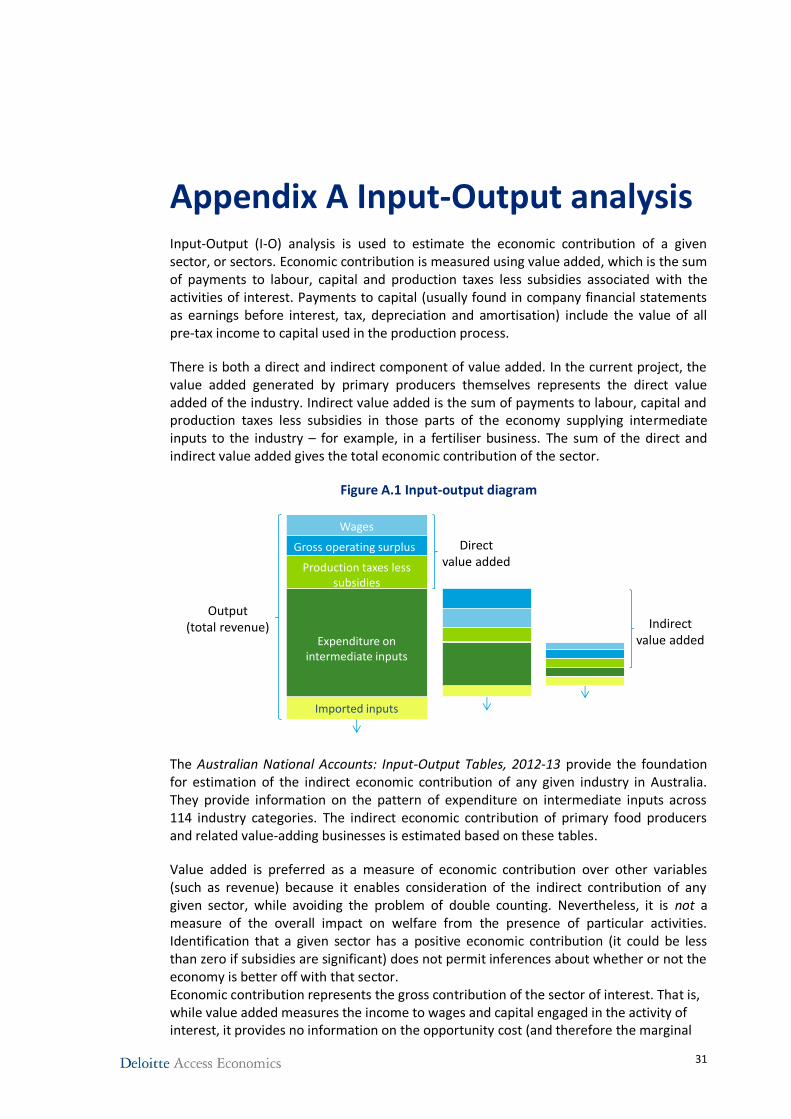
31

Appendix A Input-Output analysis Input-Output (I-O) analysis is used to estimate the economic contribution of a given sector, or sectors. Economic contribution is measured using value added, which is the sum of payments to labour, capital and production taxes less subsidies associated with the activities of interest. Payments to capital (usually found in company financial statements as earnings before interest, tax, depreciation and amortisation) include the value of all pre-tax income to capital used in the production process.

There is both a direct and indirect component of value added. In the current project, the value added generated by primary producers themselves represents the direct value added of the industry. Indirect value added is the sum of payments to labour, capital and production taxes less subsidies in those parts of the economy supplying intermediate inputs to the industry – for example, in a fertiliser business. The sum of the direct and indirect value added gives the total economic contribution of the sector.

Figure A.1 Input-output diagram

The Australian National Accounts: Input-Output Tables, 2012-13 provide the foundation for estimation of the indirect economic contribution of any given industry in Australia. They provide information on the pattern of expenditure on intermediate inputs across 114 industry categories. The indirect economic contribution of primary food producers and related value-adding businesses is estimated based on these tables.

Value added is preferred as a measure of economic contribution over other variables (such as revenue) because it enables consideration of the indirect contribution of any given sector, while avoiding the problem of double counting. Nevertheless, it is not a measure of the overall impact on welfare from the presence of particular activities. Identification that a given sector has a positive economic contribution (it could be less than zero if subsidies are significant) does not permit inferences about whether or not the economy is better off with that sector. Economic contribution represents the gross contribution of the sector of interest. That is, while value added measures the income to wages and capital engaged in the activity of interest, it provides no information on the opportunity cost (and therefore the marginal

Wages

Direct value added

Gross operating surplus

Production taxes less subsidies

Expenditure on intermediate inputs

Indirect value added

Output(total revenue)

Imported inputs

32

welfare benefits) of having those labour and capital resources utilised in the sector of interest. This means that economic contribution analysis does not permit inferences about counterfactual scenarios – for example, what might happen to living standards in the absence of the sector of interest.

33

Appendix B CGE modelling The Deloitte Access Economics – Regional General Equilibrium Model (DAE-RGEM) is a large scale, dynamic, multi-region, multi-commodity computable general equilibrium model of the world economy with bottom-up modelling of Australian regions. The model allows policy analysis in a single, robust, integrated economic framework. This model projects changes in macroeconomic aggregates such as GDP, employment, export volumes, investment and private consumption. At the sectoral level, detailed results such as output, exports, imports and employment are also produced.

Detailed description of DAE-RGEM

The model is based upon a set of key underlying relationships between the various components of the model, each which represent a different group of agents in the economy. These relationships are solved simultaneously, and so there is no logical start or end point for describing how the model actually works. However, they can be viewed as a system of interconnected markets with appropriate specifications of demand, supply and the market clearing conditions that determine the equilibrium prices and quantity produced, consumed and traded.

DAE-RGEM is based on a substantial body of accepted microeconomic theory. Key assumptions underpinning the model are:

• The model contains a ‘regional consumer’ that receives all income from factor payments (labour, capital, land and natural resources), taxes and net foreign income from borrowing (lending).

• Income is allocated across household consumption, government consumption and savings so as to maximise a Cobb-Douglas (C-D) utility function.

• Household consumption for composite goods is determined by minimising expenditure via a CDE (Constant Differences of Elasticities) expenditure function. For most regions, households can source consumption goods only from domestic and imported sources. In the Australian regions, households can also source goods from interstate. In all cases, the choice of commodities by source is determined by a CRESH (Constant Ratios of Elasticities Substitution, Homothetic) utility function.

• Government consumption for composite goods, and goods from different sources (domestic, imported and interstate), is determined by maximising utility via a C-D utility function.

• All savings generated in each region are used to purchase bonds whose price movements reflect movements in the price of creating capital.

• Producers supply goods by combining aggregate intermediate inputs and primary factors in fixed proportions (the Leontief assumption). Composite intermediate inputs are also combined in fixed proportions, whereas individual primary factors are combined using a CES production function.

34

• Producers are cost minimisers, and in doing so, choose between domestic, imported and interstate intermediate inputs via a CRESH production function.

• The supply of labour is positively influenced by movements in the real wage rate governed by an elasticity of supply.

• Investment takes place in a global market and allows for different regions to have different rates of return that reflect different risk profiles and policy impediments to investment. A global investor ranks countries as investment destinations based on two factors: global investment and rates of return in a given region compared with global rates of return. Once the aggregate investment has been determined for Australia, aggregate investment in each Australian sub-region is determined by an Australian investor based on: Australian investment and rates of return in a given sub-region compared with the national rate of return.

• Once aggregate investment is determined in each region, the regional investor constructs capital goods by combining composite investment goods in fixed proportions, and minimises costs by choosing between domestic, imported and interstate sources for these goods via a CRESH production function.

• Prices are determined via market-clearing conditions that require sectoral output (supply) to equal the amount sold (demand) to final users (households and government), intermediate users (firms and investors), foreigners (international exports), and other Australian regions (interstate exports).

• For internationally-traded goods (imports and exports), the Armington assumption is applied whereby the same goods produced in different countries are treated as imperfect substitutes. But, in relative terms, imported goods from different regions are treated as closer substitutes than domestically-produced goods and imported composites. Goods traded interstate within the Australian regions are assumed to be closer substitutes again.

• The model accounts for greenhouse gas emissions from fossil fuel combustion. Taxes can be applied to emissions, which are converted to good-specific sales taxes that impact on demand. Emission quotas can be set by region and these can be traded, at a value equal to the carbon tax avoided, where a region’s emissions fall below or exceed their quota.

Below is a description of each component of the model and key linkages between components

Households

Each region in the model has a so-called representative household that receives and spends all income. The representative household allocates income across three different expenditure areas: private household consumption; government consumption; and savings.

The representative household interacts with producers in two ways. First, in allocating expenditure across household and government consumption, this sustains demand for

35

production. Second, the representative household owns and receives all income from factor payments (labour, capital, land and natural resources) as well as net taxes. Factors of production are used by producers as inputs into production along with intermediate inputs. The level of production, as well as supply of factors, determines the amount of income generated in each region.

The representative household’s relationship with investors is through the supply of investable funds – savings. The relationship between the representative household and the international sector is twofold. First, importers compete with domestic producers in consumption markets. Second, other regions in the model can lend (borrow) money from each other.

• The representative household allocates income across three different expenditure areas – private household consumption; government consumption; and savings – to maximise a Cobb-Douglas utility function.

• Private household consumption on composite goods is determined by minimising a CDE (Constant Differences of Elasticities) expenditure function. Private household consumption on composite goods from different sources is determined by a CRESH (Constant Ratios of Elasticities Substitution, Homothetic) utility function.

• Government consumption on composite goods, and composite goods from different sources, is determined by maximising a Cobb-Douglas utility function.

• All savings generated in each region is used to purchase bonds whose price movements reflect movements in the price of generating capital.

Producers

Apart from selling goods and services to households and government, producers sell products to each other (intermediate usage) and to investors. Intermediate usage is where one producer supplies inputs to another’s production. For example, coal producers supply inputs to the electricity sector.

Capital is an input into production. Investors react to the conditions facing producers in a region to determine the amount of investment. Generally, increases in production are accompanied by increased investment. In addition, the production of machinery, construction of buildings and the like that forms the basis of a region’s capital stock, is undertaken by producers. In other words, investment demand adds to household and government expenditure from the representative household, to determine the demand for goods and services in a region.

Producers interact with international markets in two main ways. First, they compete with producers in overseas regions for export markets, as well as in their own region. Second, they use inputs from overseas in their production.

• Sectoral output equals the amount demanded by consumers (households and government) and intermediate users (firms and investors) as well as exports.

• Intermediate inputs are assumed to be combined in fixed proportions at the composite level. As mentioned above, the exception to this is the electricity sector that is able to substitute different technologies (brown

36

coal, black coal, oil, gas, hydropower and other renewables) using the ‘technology bundle’ approach developed by ABARE (1996).

• To minimise costs, producers substitute between domestic and imported intermediate inputs is governed by the Armington assumption as well as between primary factors of production (through a CES aggregator). Substitution between skilled and unskilled labour is also allowed (again via a CES function).

• The supply of labour is positively influenced by movements in the wage rate governed by an elasticity of supply is (assumed to be 0.2). This implies that changes influencing the demand for labour, positively or negatively, will impact both the level of employment and the wage rate. This is a typical labour market specification for a dynamic model such as DAE-RGEM. There are other labour market ‘settings’ that can be used. First, the labour market could take on long-run characteristics with aggregate employment being fixed and any changes to labour demand changes being absorbed through movements in the wage rate. Second, the labour market could take on short-run characteristics with fixed wages and flexible employment levels.

Investors

Investment takes place in a global market and allows for different regions to have different rates of return that reflect different risk profiles and policy impediments to investment. The global investor ranks countries as investment destination based on two factors: current economic growth and rates of return in a given region compared with global rates of return.

• Once aggregate investment is determined in each region, the regional investor constructs capital goods by combining composite investment goods in fixed proportions, and minimises costs by choosing between domestic, imported and interstate sources for these goods via a CRESH production function.

International Each of the components outlined above operate, simultaneously, in each region of the model. That is, for any simulation the model forecasts changes to trade and investment flows within, and between, regions subject to optimising behaviour by producers, consumers and investors. Of course, this implies some global conditions that must be met, such as global exports and global imports, are the same and that global debt repayment equals global debt receipts each year.

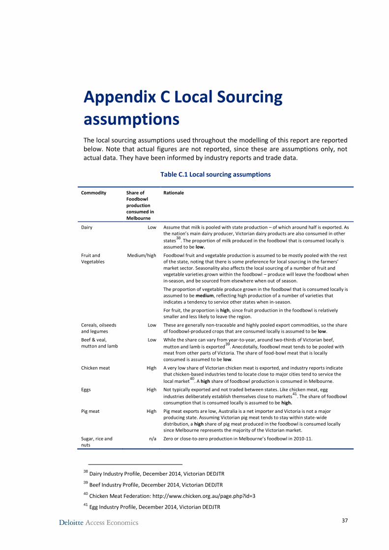
37

Appendix C Local Sourcing assumptions The local sourcing assumptions used throughout the modelling of this report are reported below. Note that actual figures are not reported, since these are assumptions only, not actual data. They have been informed by industry reports and trade data.

Table C.1 Local sourcing assumptions

Commodity Share of Foodbowl production consumed in Melbourne

Rationale

Dairy Low Assume that milk is pooled with state production – of which around half is exported. As the nation’s main dairy producer, Victorian dairy products are also consumed in other

states38

. The proportion of milk produced in the foodbowl that is consumed locally is assumed to be low.

Fruit and Vegetables

Medium/high Foodbowl fruit and vegetable production is assumed to be mostly pooled with the rest of the state, noting that there is some preference for local sourcing in the farmers’ market sector. Seasonality also affects the local sourcing of a number of fruit and vegetable varieties grown within the foodbowl – produce will leave the foodbowl when in-season, and be sourced from elsewhere when out of season.

The proportion of vegetable produce grown in the foodbowl that is consumed locally is assumed to be medium, reflecting high production of a number of varieties that indicates a tendency to service other states when in-season.

For fruit, the proportion is high, since fruit production in the foodbowl is relatively smaller and less likely to leave the region.

Cereals, oilseeds and legumes

Low These are generally non-traceable and highly pooled export commodities, so the share of foodbowl-produced crops that are consumed locally is assumed to be low.

Beef & veal, mutton and lamb

Low While the share can vary from year-to-year, around two-thirds of Victorian beef,

mutton and lamb is exported39

. Anecdotally, foodbowl meat tends to be pooled with meat from other parts of Victoria. The share of food-bowl meat that is locally consumed is assumed to be low.

Chicken meat High A very low share of Victorian chicken meat is exported, and industry reports indicate that chicken-based industries tend to locate close to major cities tend to service the

local market40

. A high share of foodbowl production is consumed in Melbourne.

Eggs High Not typically exported and not traded between states. Like chicken meat, egg

industries deliberately establish themselves close to markets41

. The share of foodbowl consumption that is consumed locally is assumed to be high.

Pig meat High Pig meat exports are low, Australia is a net importer and Victoria is not a major producing state. Assuming Victorian pig meat tends to stay within state-wide distribution, a high share of pig meat produced in the foodbowl is consumed locally since Melbourne represents the majority of the Victorian market.

Sugar, rice and nuts

n/a Zero or close-to-zero production in Melbourne’s foodbowl in 2010-11.

38 Dairy Industry Profile, December 2014, Victorian DEDJTR

39 Beef Industry Profile, December 2014, Victorian DEDJTR

40 Chicken Meat Federation: http://www.chicken.org.au/page.php?id=3

41 Egg Industry Profile, December 2014, Victorian DEDJTR

38

References

Australian Bureau of Statistics (ABS) (2012), Value of agricultural commodities produced, 2010–11, available at http://www.abs.gov.au/ausstats/abs@.nsf/mf/7503.0.

ABS (2012), Census of population and housing, 2011, available at http://www.abs.gov.au/census.

Australian Competition and Consumer Commission (2008), Report of the ACCC inquiry into the competitiveness of retail prices for standard groceries, Australian Competition and Consumer Commission, Canberra.

Australian Chicken Meat Federation (2016), Locations of farms and processing plants, available at http://www.chicken.org.au/page.php?id=3.

Buxton, M., Hurley, J. and Phelan, K. (2015), Melbourne at 8 million: matching land supply to dwelling demand, Centre for Urban Research, RMIT University, October.

Carey, R., Larsen, K. and Sheridan, J. (2015), The role of cities in climate resilient food systems: A Foodprint Melbourne briefing, Victorian Eco-Innovation Lab, The University of Melbourne.

City of Whittlesea (2011), Whittlesea Green Wedge Management Plan 2011-21, available at https://www.whittlesea.vic.gov.au/building-planning-and-transport/planningdev/planning-for-the-future/green-wedge-management-plan.

Conner, D., Becot, F., Hoffer, D., Kahler, E., Sawyer, S. and Berlin, L. (2012), Measuring current consumption of locally grown foods in Vermont: Methods for baselines and targets, Journal of Agriculture, Food Systems and Community Development, available at http://mainefoodstrategy.com/wp-content/uploads/2013/05/jafscd_measuring_local_food_consumption_vermont_may-2013.pdf.

Department of Transport, Planning and Local Infrastructure Victoria (2016), Green Wedges, available at http://www.dtpli.vic.gov.au/planning/plans-and-policies/green-wedges.

Department of Economic Development, Jobs, Transport and Resources (DEDJTR) (2016), Dairy Industry Profile, December (2014), Agriculture Victoria, available at http://agriculture.vic.gov.au/agriculture/food-and-fibre-industries/industry-profiles.

DEDJTR (2016), Beef Industry Profile, December (2014), Agriculture Victoria, available at http://agriculture.vic.gov.au/agriculture/food-and-fibre-industries/industry-profiles.

DEDJTR (2016), Egg Industry Profile, December (2014), Agriculture Victoria, available at http://agriculture.vic.gov.au/agriculture/food-and-fibre-industries/industry-profiles.

Department of Environment, Land, Water & Planning (2015), Victoria in Future 2015, available at http://www.dtpli.vic.gov.au/data-and-research/population/victoria-in-future-2016.

39

Ecker, S., Clarke, R., Cartwright, S., Kancans, R., Please, P. and Binks, B. (2010), Drivers of regional agritourism and food tourism in Australia, Australian Bureau of Agricultural and Resource Economics – Bureau of Rural Sciences report, Canberra.

Gardner, B. (1977), The economics of agricultural land preservation, American Journal of Agricultural Economics, Vol. 59 No. 5 pp1027-1036.

Garnaut, R. (2011), The Garnaut Review 2011: Australia in the Global Response to Climate Change, available at http://www.garnautreview.org.au/update-2011/garnaut-review-2011/summary-20June.pdf.

Henderson, S. and Epps, R. (2000), Urban Fringe Land Use Conflict: Two Case Studies, A report for the Rural Industries Research and Development Corporation, Human and Environmental Studies, University of New England, Armidale.

Kline, J. and Wilchens, D. (1996), Public preferences regarding the goals of farmland preservation programs, Land Economics, Vol. 72, pp538-549; Nickerson, C.J. and Hellerstein, D. (2003), Protecting rural amenities through farmland preservation programs, Agricultural and Resource Economics Review, Vol. 32, pp129-144.

Marquez, L., Higgins, A. and Estrada-Flores, S. (2010), Understanding Victoria’s Fruit and Vegetable Freight Movements, Report for the Victorian Eco-Innovation Lab, The University of Melbourne, available at http://www.ecoinnovationlab.com/wp-content/attachments/398_Understanding-Vic-FV-Freight-Movements.pdf.

Martinez, S., Hand, M., Da Pra, M., Pollack, S., Ralston, K., Smith, T., Vogel, S., Clark, S., Lohr, L., Low, S. and Newman, C. (2010), Local Food Systems: Concepts, Impacts, and Issues, United States Department of Agriculture Economic Research Service, Economic Research Report Number 97.

Masi, B., Shaller, L. and Shuman, M. H. (2010), The 25% shift: the benefits of food localization for Northeast Ohio & how to realise them, available at http://www.neofoodweb.org/sites/default/files/resources/the25shift-foodlocalizationintheNEOregion.pdf.

Melbourne and Metropolitan Board of Works (1971), Planning Policies for Metropolitan Melbourne.

Metropolitan Planning Authority (2016), Precinct Structure Plans (PSPs), Victoria State Government available at http://www.mpa.vic.gov.au/planning-activities/greenfields-planning/precinct-structure-plans/.

Ollenburg, C. (2006), Farm Tourism in Australia: A Family Business and Rural Studies Perspective, PhD thesis, School of Environmental and Applied Sciences, Faculty of Environmental Sciences, Griffith University.

Sheridan, J., Carey, R. and Candy, S. (2016), Melbourne’s Foodprint: What does it take to feed a city?, Victorian Eco-Innovation Lab, The University of Melbourne, available at http://www.ecoinnovationlab.com/wp-content/attachments/Foodprint-Melb-What-it-takes-to-feed-a-city.pdf.

40

Timmons, D., Wang, Q. and Lass, D. (2008), Local Foods: Estimating Capacity, Journal of Extension, vol 46 (5), available at http://www.joe.org/joe/2008october/a7.php.

41

Limitation of our work

General use restriction

This report is prepared solely for the use of the University of Melbourne. This report is not intended to and should not be used or relied upon by anyone else and we accept no duty of care to any other person or entity. The report has been prepared for the purpose of assisting the University of Melbourne in providing an economic contribution of Melbourne’s foodbowl. You should not refer to or use our name or the advice for any other purpose.

Contact us

Deloitte Access Economics ACN: 149 633 116 8 Brindabella Circuit Brindabella Business Park Canberra Airport ACT 2609 Tel: +61 2 6263 7000 Fax: +61 2 6263 7004 www.deloitteaccesseconomics.com.au

Deloitte Access Economics is Australia’s pre-eminent economics advisory practice and a member of Deloitte's global economics group. The Directors and staff of Access Economics joined Deloitte in early 2011.

About Deloitte

Deloitte refers to one or more of Deloitte Touche Tohmatsu Limited, a UK private company limited by guarantee, and its network of member firms, each of which is a legally separate and independent entity. Please see www.deloitte.com/au/about for a detailed description of the legal structure of Deloitte Touche Tohmatsu Limited and its member firms.

Deloitte provides audit, tax, consulting, and financial advisory services to public and private clients spanning multiple industries. With a globally connected network of member firms in more than 150 countries, Deloitte brings world-class capabilities and deep local expertise to help clients succeed wherever they operate. Deloitte's approximately 200,000 professionals are committed to becoming the standard of excellence.

About Deloitte Australia

In Australia, the member firm is the Australian partnership of Deloitte Touche Tohmatsu. As one of Australia’s leading professional services firms. Deloitte Touche Tohmatsu and its affiliates provide audit, tax, consulting, and financial advisory services through approximately 6,000 people across the country. Focused on the creation of value and growth, and known as an employer of choice for innovative human resources programs, we are dedicated to helping our clients and our people excel. For more information, please visit our web site at www.deloitte.com.au.

Liability limited by a scheme approved under Professional Standards Legislation.

Member of Deloitte Touche Tohmatsu Limited

© 2016 Deloitte Access Economics Pty Ltd