Embed Size (px)
Citation preview

The Economic Effects of a Borrower Bailout:Evidence from an Emerging Market∗
Xavier Gine† Martin Kanz‡
November 18, 2013
***Preliminary. Please do not cite or circulate without permission.***
Abstract
Economic stimulus programs that operate through the credit market may give rise to partic-ularly severe moral hazard problems because they change the contracting environment anddistort borrower incentives. We test this proposition using a natural experiment arising froma nationwide bailout program for highly-indebted households in India. Our empirical strategyexploits local variation in cross-sectional exposure to the program, as measured by the shareof qualifying loans at the time of the program announcement. We find that the programgenerated no measurable productivity gains, but led to significant moral hazard in loan re-payment. Post-program loan performance declines faster in districts with greater exposure tothe program, an effect that is not driven by greater risk-taking of banks. In addition, loandefaults become significantly more sensitive to the electoral cycle in the post-program period.This suggests that expectations of future credit market interventions generated by the bailoutare an important channel through which moral hazard in loan repayment is intensified.
JEL: G21, G28, O16, O23Keywords: bailout, rural credit, economic stimulus, moral hazard
∗We thank the Reserve Bank of India and several State Level Bankers’ Committees for sharing data used in this paper.
Maulik Chauhan and Avichal Mahajan provided outstanding research asistance. Financial assistance from the World Bank
Research Support Budget is gratefully acknowledged. The opinions expressed do not necessarily represent the views of the
World Bank, its Executive Directors, or the countries they represent.
† The World Bank, Development Research Group, 1818 H Street NW, Washington, DC 20433. Email: [email protected]
‡ The World Bank, Development Research Group, Email: [email protected]
1 Introduction
Economic stimulus programs have been used in a wide variety of economic contexts the world
over in an effort to spur economic activity. The fundamental question of whether governments
can improve economic outcomes through such programs, however, remains controversial and
has received heightened attention in the wake of the 2008 global economic crisis. While
economists in the “Keynesian” tradition advocate government interventions to increase ag-
gregate demand and reduce the negative externalities of a prolonged economic downturn
for society (Campbell et al. [2011], Mian et al. [2010]), critics argue that fiscal stimulus
programs create the potential for political capture and moral hazard and can have adverse
distributional consequences (Agarwal et al. [2013]).
A more nuanced version of this debate considers the comparative merits of different types
of economic stimulus programs. In its simplest form, a stimulus program provides direct
subsidies or income support to firms and individuals. In many cases, however, stimulus
programs operate through the credit market, for example in the form of mandated debt
restructuring programs or the public takeover of private liabilities.
The economic argument in favor of stimulus programs operating through the credit mar-
ket rests on the premise that such policies will prevent excessive deadweight losses from
foreclosure in settings where contracts are incomplete and market participants are unable
to insure against macroeconomic shocks (Bolton and Rosenthal [2002]). Opponents of this
view argue that political interventions in the credit market are a particularly harmful way of
implementing stimulus programs because they change the contracting environment and are
likely to give rise to moral hazard problems by distorting borrower expectations. Although
this is ultimately an empirical question, very little evidence exists on the effect of such poli-
cies on credit supply and ex-post borrower behavior despite the fact that credit-market led
stimulus programs are ubiquitous.
1

We shed light on these issues by analyzing one of the largest household debt relief pro-
grams in history, enacted by the government of India in 2008 against the backdrop of the
global economic crisis. The program, known as the Agricultural Debt Waiver and Debt
Relief Scheme (ADWDRS) consisted of unconditional debt relief for more than 60 million
rural households and amounted to a volume of more than US$ 16 billion or 1.7% of GDP.
India’s ADWDRS program is an especially attractive testing ground to explore the impact
of a stimulus program on credit market outcomes for several reasons. First, the program is
quite representative of a wide range of stimulus programs executed through policy interven-
tions in the credit market. In the United States, several states intervened into debt contracts
by passing debt moratoria intended to prevent excessive foreclosures and to protect rural
constituencies from the fallout of the Great Depression (Rucker and Alston [1987]). More
recent interventions in debt contracts in the United States include programs for mortgage
renegotiation in response to the foreclosure crisis of 2008 (Agarwal et al. [2013], Guiso et al.
[2013]). In developing countries, governments have routinely implemented debt relief and
debt restructuring programs, often targeted at the economically important and politically
influential rural sector. Some recent examples include a US$ 2.9 billion bailout for farmers
in Thailand and the restructuring of more than US$10 billion of household debt in Brazil.
Second, unlike many other political interventions in the credit market, it was a one-off initia-
tive that left the formal institutional and regulatory environment unchanged, thus allowing
us to isolate the effect of the capital injection. But perhaps more importantly, unlike any
of the previous debt relief initiatives in India, eligibility for the bailout program depended
on the amount of land pledged at the time of loan origination, typically many years prior to
the program. This rule, applied retrospectively, implies that the share of credit that could
qualify for the program is a function of the land distribution in a given district. The land
distribution in turn interacts with the time series of productivity shocks faced by a given
district to determine the share of qualifying credit that was actually in default at the time
2

the program was introduced.
Our empirical strategy exploits this exogenous geographical variation in program expo-
sure at the district level to identify the causal impacts of the bailout on ex-post credit supply
and borrower behavior. Using public and proprietary data on bank lending and loan perfor-
mance, we construct a new dataset tracing credit allocation and loan delinquencies for 491
districts of India over the period 2001-2012. We match these data with information on the
amount of debt relief as a share of total credit allocated in each district, which forms our
primary measure of program exposure. The data reveal substantial variation in exposure
to the debt relief program with the share of total credit waived under the program ranging
from an average of less than 3% in some districts of the state of Goa to more than 50% of
total credit in many districts of the states of Bihar, Jharkand, Orissa and Uttar Pradesh.
Our baseline estimates indicate that the bailout had a significant and economically large
effect on post program credit allocation. These effects are larger in areas with greater
exposure to the bailout, and robust to alternative specifications and construction of the
variable measuring treatment intensity. A one standard deviation in the share of bailout
leads to an increase in the growth rate of agricultural credit of 12.5% but no discernible
increase in the number of accounts, indicating that additional credit was disbursed to existing
customers in good standing. This suggests that banks acted conservatively by not expanding
the customer base. Following the loan waiver program, however, defaults increased, either
because borrower discipline declined (moral hazard) or because borrowers’ debt burden had
increased as the loan size was larger. To disentangle both explanations, we focus on defaults
and disbursements around elections and find that while defaults increase before elections
after the loan waiver, there is no such increase in disbursements. We thus conclude that
moral hazard is the more likely explanation for the rise in defaults. Consistent with this
explanation, we find no evidence of improvements in agricultural productivity following the
loan waiver.
3

These results contribute to several strands of the literature. To the best of our knowledge,
we provide the first empirical evidence on the aggregate credit market and moral hazard
implications of large-scale debt relief programs. In this sense our findings contribute to a
nascent literature on the market response and broader economic impact of stimulus programs.
Agarwal et al. [2013] study subsidized mortgage renegotiations under the Home Affordability
Modification Program in the wake of the foreclosure crisis in the United States, and Mian and
Sufi [2012] study the impact of a stimulus program offering subsidies for new car purchases
on auto sales and broader economic outcomes. Our analysis differs from this literature as it
focuses on a stimulus initiative enacted through credit market, considering its direct effect on
subsequent lending on the intensive and extensive margins, and post-program moral hazard
in loan repayment.
Because the bailout affected not only borrowers but was also tied to a recapitalization
of banks refinanced by the Reserve Bank of India as part of ADWDRS, our results are also
related to the literature on the real effects of bank recapitalizations (Diamond and Rajan
[2000], Paravisini [2008], Philippon and Schnabl [2013] and Gianetti and Simonov [2013]).
There is much reason to believe that prior to the announcement of ADWDRS, Indian banks
faced significant incentives for evergreening de-facto non-performing loans. Reflecting a long
history of directed lending (Burgess and Pande [2005], Cole [2009a]), all banks in India are
required to lend 40% of their capital to “priority sectors”, which include agriculture and small
scale industry. Although this mandate forced the allocation of a significant share of credit to
high-risk borrowers, local branches and branch managers faced sanctions for realizing losses
and consequently had a significant incentive to keep lending to defaulters. The introduction
of ADWDRS removed this incentive distortion. Consistent with the evergreening hypothesis
(Peek and Rosengren [2005]), we find evidence of a shift in post-program lending away from
districts with a high-share of total credit waived under the bailout. Indeed, one dollar of
bailout led to an increase in net lending in subsequent years of only 9 cents in a high-bailout
4

district and almost 70 cents in a low-bailout district. This suggests that the bailout did not
encourage greater risk-taking by banks and thus helps us isolate the effect of ADWDRS on
bank risk-taking from its impact on borrower behavior. Despite the geographical reallocation
of new lending towards districts with observably lower ex-ante risk, we find a significant
negative effect of the program on loan performance, concentrated among borrowers that had
previously been in good standing and who did not benefit from the bailout.
Finally, the finding that loan performance (but not loan size) is responsive to the electoral
cycle and that this effect is magnified by the introduction of the ADWDRS bailout program
contributes to the literature on the political economy of credit in emerging markets (Cole
(2009), Dinc (2005)) and underscores the concern with stimulus programs that they may lead
to an anticipation of future interventions, especially in credit markets that have a history of
political intervention.
The rest of the paper proceeds as follows. In Section 2, we provide an overview over the
eligibility rules and timing of India’s bailout program for rural households. Section 3 pro-
vides details about the data used and provides summary statistics. In Section 4 we discuss
our empirical strategy and in ction 5 we present the results. Section 6 concludes.
2 India’s Bailout Program for Rural Households
We study the impact of debt relief on credit supply and borrower moral hazard using a
natural experiment generated by India’s “Agricultural Debt Waiver and Debt Relief Program
for Small and Marginal Farmers” or ADWDRS, one of the largest borrower bailout programs
in history enacted by India’s federal government and executed by the Reserve Bank of India
beginnning in March 2008.
The goal of the program was to refinance all private, public sector, cooperative and re-
gional rural banks through the cancellation of their non-performing rural assets accumulated
5

due to the long history of directed lending to the rural sector. In turn, this reduction of
household debt would serve as stimulus against the debt overhang and lack of access to
credit among highly indebted rural households. Given that the bailout was announced a
year ahead of national elections, the program also acted as a significant transfer from urban
to rural voters.
The rules for program eligibility were kept deliberately simple to allow for the swift pro-
cessing of claims, and to minimize corruption at local bank branches tasked with identifying
eligible borrowers. In contrast to earlier debt relief initiatives, eligibility for the program at
the level of an individual loan depended on the amount of land pledged as collateral at the
time a loan was originated, typically several years before the program. Small borrowers who
had pledged less than two hectares of land were eligible for full debt relief, while borrowers
with overdue loans that had pledged more than two hectares of land qualified for 25% condi-
tional debt relief if they were able to repay the remaining balance. Loans qualified for debt
relief if they were originated between December 31, 1997 and December 31, 2007, more than
90 days overdue as of December 31, 2007 and remained in default until February 28, 2008.
These rules were announced retrospectively in the Indian finance minister’s budget speech
on March 18, 2008 so that there was no scope for manipulation around program dates. In
addition, it was the first time that eligibility was based on landholdings and thus the rules
were unanticipated.
Implementation of the program began in June 2008. Every bank branch in the country
was asked to identify all loans and borrowers on its books that met the bailout eligibility
criteria. As a transparency measure, branches were required to publicly post these beneficiary
lists, including the identity of the borrower as well as the details of the qualifying loan.
Borrower lists underwent independent audits at the branch and bank level and an appeals
process was put in place to allow borrowers a way to rectify errors in published beneficiary
lists. Unconditional debt relief, which accounted for approximately 81% of claims, was
6

processed immediately so that virtually all claims had been settled by the end of June 2008.
In contrast, the deadline for settling claims under the partial debt relief scheme for loans
with collateral of more than two hectares of land was extended several times because of slow
take-up –first to December 2009, and subsequently to December 2010. To ensure that we
accurately capture the total amount of debt relief granted in a district, we use data as of
December 2011, when the program was closed and all claims had been settled.
3 Data
Our dataset includes 489 districts for which we have information on debt relief amounts,
as well as detailed credit outcomes and agricultural productivity data for the years 2001 to
2012. We aggregate all data to the level of an administrative district. In the base year 2001,
India had 593 districts with an average population of 1,731,897 inhabitants. In that year
the districts in our sample account for 94% of the Indian population and 89% of total bank
credit.1
How did exposure to the bailout affect ex-post credit supply and borrower behavior? The
key challenge we need to overcome to address this question is to form a credible control group
that was not affected by the program. But because all districts were affected we define a
continuous treatment variable measuring program exposure rather than classifying districts
into treatment and control groups. We then form counterfactuals using the cross-sectional
variation in program exposure.
To measure a district’s exposure to the bailout, we collected data on the amount of debt
relief granted under the program from each state’s State Level Bankers’ Committee, the
administrative body responsible for maintaining regionally disaggregated data on publicly
supported credit market interventions. Using these data we construct a variable measuring
1We have bank credit data for a total of 501 districts but in the analysis we drop 10 districts thatcorrespond to the largest urban areas and 2 districts in Jammu and Kashmir that have virtually no bankpenetration.
7

the share of outstanding credit waived under the program in each of the 491 districts in
our sample. Specifically, let creditdt denote the total amount of outstanding rural credit in
district d at the time of the program deadline t on February 28, 2008, with superscript S
denoting the share of debt owed by households below the two hectare eligibility cutoff and
superscript L denoting debt owed by households above the cutoff. Letting η denote the
share of rural credit that was current at the program deadline and therefore unaffected by
the program, district d’s exposure to the program is equivalent to:
Bailout sharedt =(1− η)
[creditSdt + .25κdcreditLdt
]creditSdt + creditLdt
(1)
where κd denotes the fraction of loans settled under the partial debt relief option for
households above the two hectare cutoff. Because settlement was optional for households
above the two hectare cutoff, our baseline estimates assume κd = 1, which is equivalent
to estimating the intent-to-treat (ITT) effect for households with more than two hectares
of land pledged as collateral.2 To ensure that our measure of program exposure includes
all debt waiver allocations under the program,the variable is calculated with administrative
data reported in December 2011, after the program had officially closed and all allocations
had been made.
Table I reports summary statistics for the share of credit written off under the program
and highlights significant geographical variation in program exposure. The mean (median)
district in our sample saw 32.6% (28.4%) of outstanding credit waived under the program.
Bailout shares at the state level are reported in Appendix B and range from 2.2% in Goa to
2 Because debt relief was automatic for households below the cutoff, the intent-to-treat (ITT) and
treatment-on-treated (TOT) estimates are identical for households with pledged landholdings below two
hectares.
8

more than 60% in Orissa.
Data on credit are taken from the Reserve Bank of India’s Basic Statistical Returns of
Commercial Banks. Each year, all bank branches in India are required to report details of
all loans on their books to the regulator. This annual ‘census’ of outstanding credit includes,
for each district, details on the sectoral allocation of credit, interest rates, loan amounts
and number of outstanding loans as of March 31st, the end of the Indian fiscal year. We
use this geographically disaggregated dataset for the years 2001 to 2012 to construct time
series of outstanding credit (amount and number of loans) for each district and for various
types of credit. Figure 1 plots the growth in agricultural credit year by year. While credit
outstanding continues to grow at the same rate before and after the program, the growth in
the number of new accounts declines, suggesting that banks become more conservative when
issuing new loans. And since disbursement is growing, average loan sizes must have increased
for the relatively fewer individuals that have managed to borrow after the program.
Estimating the impact of the program on ex-post borrower behavior requires detailed
information on loan performance. Because data on loan performance is not disclosed by the
regulator at a regionally disaggregated level, we use a new proprietary dataset of lending and
loan performance of India’s five largest commercial banks. The dataset contains information
on the number of loans and the volume of total/non-performing loans, disaggregated by
bank and district for the years 2006 to 2012 and covers data from 27,678 bank branches,
which account for approximately 62% of total agricultural credit. Figure 2 plots the year
by year share of non-performing loans. Interestingly, there is a surge in NPLs from 2007 to
2008, possibly because Indian banks responded to the program by converting into default
loans that were previously ever-greened. Indeed, the mandate to lend 40% of capital to
“priority sectors”, including agriculture, and the sanctions that local branch managers face
for realizing losses creates an incentive to evergreen the loans of defaulters. Once the program
is announced, these loans can be shown as non-performing in the books so that they will be
9

covered by the waiver program. Mechanically, after the program the share of NPLs decline
sharply as defaults are waived, but over time NPLs raise again.
Data on agricultural productivity come from the Indian Ministry of Agriculture’s database
on crop yields. We use 2001 commodity prices from Indiastat to construct the value of agri-
cultural production per hectare in a given district and year. Appendix C provides additional
details on the construction of the productivity series.
The analysis controls for exogenous changes in credit conditions using local variation in
monsoon rainfall. Rainfall data were obtained from the Indian Meteorological Department
and measure monthly precipitation based on rainfall gauges located in each district. The
rainfall variable we use in our analysis is total monsoon rainfall between July and Septem-
ber for the previous year as a fraction of the district’s long-run rainfall average over the
same period. The analysis also controls for the district’s distance to the next scheduled
state election by including a full set of electoral cycle dummies. Electoral data come from
the Election Commission of India’s database on state elections.3 Finally, we use data on
district characteristics from the Census of India and the Indian Agriculture Census. These
data include the total population, urban and rural population shares, productivity and land
distribution of each district. We provide additional details on the construction of variables
in Appendix A. Summary statistics are reported in Table II.
4 Empirical Strategy
To assess the impact of the bailout on credit supply and ex-post borrower behavior we
exploit variation in debt relief at the district level, due to the fact that the same program
rules were applied uniformly across the country. Figure 3 plots the geographical dispersion
of the share of total outstanding rural credit that was waived under the program (Panel (a)
) and the growth in NPLs after the program (Panel (b)) by quartiles. In our analysis, we
3Available at http://eci.nic.in/eci main1/key highlights.aspx
10

treat the variation in Panel (a) as quasi-exogenous because it is determined jointly by the
district’s land-distribution, which affects the share of landholdings below the program cutoff
that could have been eligible for full debt relief, and the time series of exogenous weather
shocks in the district, which determines the share of loans actually in default at the time of
the program deadline.
Table A.I correlates program exposure with district level measures of land distribution
and rainfall. Column 1 reports a negative and significant correlation between share of in-
dividuals with landholdings below the two hectare eligibility threshold and the share of
agricultural credit waived. Column 2 includes a non-linear term and finds a weaker relation-
ship. However, a district’s land distribution is only one factor determining program intensity,
the second being the time series of exogenous income shocks which, in rural India are mostly
due to variation in the onset and intensity of the southwest monsoon. This explains why
program exposure varies not only across state lines, but also within areas with a relatively
similar land distribution, such as parts of Rajasthan and Southern Karnataka. Column 3
correlates the numer of drought years prior to the program from 2001 to 2007 with the share
of agricultural credit waived. As expected, the correlation is positive. More interestingly,
columns 4 and 5 include a linear term to proxy for land distribution (column 4) or a linear
and a quadratic term (column 5), the number of drought years and its interaction. The
coefficient of the interaction is positive and significant suggesting that both the district’s
historically determined land distribution as well as the time series of exogenous weather
shocks affect the district’s program exposure.
We use this source of quasi-exogenous variation in exposure to the ADWDRS program in
Panel (a) of Figure 3 to estimate difference-in-differences regressions that compare outcomes
across districts with different levels of program exposure before and after the bailout. Thus
we have 11 years times 489 districts minus 461 district-year observations for which we lack
a time-varing district level control, for a total of 4,918 observations. The fixed effects model
11

that we estimate is as follows:
Ydt/Yd,t−1 = α + γExposure+ δd + ϑt + X′dtζ + εdt (2)
where Ydt/Yd,t−1 is the year-on-year change in one of our outcomes of interest, such as the
number of outstanding loans, total credit or growth in NPLs, δd is a district fixed effect, ϑt
is a year dummy or district time trend and Xdt is a matrix of ime-varying district-specific
controls. Exposure is an interaction between the share of rural credit written off under
the program and a post-program dummy, which is equal to one for all years after 2008 and
zero otherwise. Hence, the coefficient γ is our differences-in-differences estimate of program
impact. To facilitate the interpretation of the estimate of γ, the variable “bailout share” is
normalized to have mean zero and standard deviation one. We estimate the model in (2) by
weighted least squares (WLS) because smaller districts may have poorer credit administrative
data and might depend on a smaller number of crops becoming more vulnerable to exogenous
shocks as a result. We construct the weights using the log of total outstanding credit in the
base year 2001 as a proxy for the size of the district economy.4. Standard errors are clustered
at the district level, the same unit of analysis at which exposure to the program is observed.
The validity of our identification strategy depends on the assumption that average changes
in outcomes in the pre- and post-program periods are unrelated to the bailout share in a
given district. This assumption would be violated if, for example, loan or credit growth
were on a different time trend in districts with greater exposure to the program. While this
assumption is fundamentally untestable, we report three different specifications to demon-
strate that the identification assumption is unlikely to be violated. At the same time, these
different specifications can be thought of as robustness checks that address other possible
4 See Strahan and Jayaratne [1996] for a similar approach
12

challenges to our identification strategy.
First, the inclusion of district fixed effects control for time-invariant differences in credit
growth and other outcomes of interests that differ due to unobserved factors at the district
level. Some examples might include differences in local public expenditure, the distribution
of land or differential exposure to price or productivity shocks. The inclusion of district fixed
effects also accounts for the possibility of mean reversion in credit and productivity growth.
Second, we account for the presence of regional credit cycles. To do this, we first include
a set of electoral cycle dummies in all of our specifications. The electoral cycle dummies
indicate the number of years until the next scheduled state election and account for the fact
that both credit and loan performance have been shown to be strongly correlated with the
electoral cycle.
In our second specification, we additionally account for the presence of regional cycles
in credit and loan performance that are unrelated to the timing of elections. This approach
reduces the likelihood that our estimate γ is biased by a correlation between program expo-
sure and the regional business cycle. We use the Reserve Bank of India’s four administrative
zones and divide India into four regions accordingly. This specification includes interactions
between year effects and regional dummies to allow for variation in regional cycles and uses
44 degrees of freedom.
Finally, we estimate a version of our core empirical model that allows each district to be on
a separate linear time trend at a cost of 489 degrees of freedom. This third specification serves
as an additional robustness check and reduces the likelihood that the estimated difference-
in-differences treatment effect γ is biased by a correlation between program exposure and
pre-existing time trends in our key outcomes of interest.
13
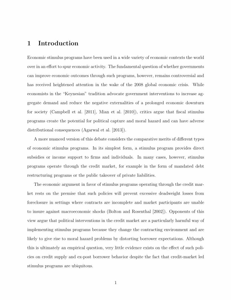
5 Results
Tables III and IV report the main results. The dependent variables in Table III relate to the
supply of credit. In columns 1-3 we regress the year on year percentage change in the number
of loans while in columns 4-6 we regress the year on year percentage change in outstanding
credit on our measure of program exposure according to specification (1), including either
year fixed effects (columns 1 and 4), time trends of district level covariates (columns 2 and
5) or individual district time trends (columns 3 and 6). Since the inclusion of district time
trends is more conservative, we take this specification as our preferred one. In addition,
all regressions control for the deviation of lagged monsoon rainfall from its normal average
since agriculture production in India is mostly rainfed and the quality of the monsoon is
likely to affect the default rate and subsequent credit growth. The regressions also control
for the number of years since the next state election because the credit market behaves
differently during election years (Cole [2009b]). All regressions include district fixed effects
and are weighted by the district’s total credit outstanding in 2001. Each cell in Tables III
and IV reports the coefficient of interest γ which corresponds to the differences-in-differences
estimate of program impact.
Panel A of Table III reports the program impact on total agricultural credit. In columns
1-3 we find that program exposure leads to no increase in the growth in the number of loans
but in columns 4-6 program exposure does lead to an increase in the growth rate of agricul-
tural credit. In particular, an increase of one standard deviation in program exposure leads
to an increase in the growth rate of agricultural credit of 3.7% according to the preferred
specification of column 6. These results suggest that new credit was given to existing cus-
tomers, most likely those that did not participate in the loan waiver and that were therefore
in good standing. In addition, it appears that banks are now lending more conservatively
after the loan waiver, which may suggest that the bailout was large enough to solve the
14

banks’ debt overhang problem (Gianetti and Simonov [2013]).
Panel B of Table III runs two types of placebo tests exploiting the timing of the program.
Instead of defining the post-program dummy as equal to one for all periods after 2008, we
restrict the sample to before 2008 and define the post-program dummy as equal to one either
after 2003 or after 2006. In neither case one cannot replicate the pattern of credit growth
found in Panel A, lending credibility to the hypothesis that the increase in the growth rate
of credit after the program is due to the program itself and not to peculiarities in the data.
Table IV explores the impact of debt relief on post-program loan performance. We rely
on unique proprietary data of non performing agricultural loans collected from each states’
State Level Banking Committee (SLBC) that are not available for non-agricultural loans.
The dependent variable is a dummy that takes value one if there is an increase in non
performing assets in a given disrict and year. Columns 1-3 use data for 489 districts while
columns 4-6 restrict the sample to 237 districts where competition among banks defined by
the number of branches in the district per capita is above the median. Using either sample
we find an increase in the probability of positive growth rate of non-performing loans. Panel
B reports the result of a placebo test where the post-program dummy is defined to take the
value one after 2007, restricting again the sample to 2008. Using this placebo post-program
dummy we find no impact on the probability of growth in defaults, suggesting again that
the program did cause the increase in defaults. However, this increase in defaults could be
due to the higher debt burden given that the loan sizes increased after the program or to
moral hazard as borrowers inferred from the waiver that future interventions might be in
store, and therefore that the consequences of default were not as severe.
Table VI helps disentangle these two mechanisms by interacting the post-program dummy
with a variable that takes on the number of years until the next state election. Panel A
reports that defaults rise closer to election years especially after the program, while in Panel
B there is no difference before or after the program in the increase in the number of loans due
15

to proximity to elections. We therefore conclude that the increase in defaults documented
in Table IV is most likely due to moral hazard, since the expectation of future bailout is
heightened in the run-up to elections.
An important aim of economic stimulus programs is to stabilize output, and to prevent
distortions in investment and consumption decisions during exceptionally harsh economic
circumstances. In the case of debt relief for rural households, it is often argued that extreme
levels of indebtedness create “debt overhang” and severe disincentives for investment, so
that economic stimulus programs enacted as debt relief hold the promise of improving the
productivity of recipient households. The ADWDRS program offers a compelling test of
this proposition. To explore the effect of debt relief on agricultural productivity, we take
advantage of detailed district level panel on commodity prices and crop yields from the Indian
Department of Agriculture. The dataset, which we describe in more detail in Appendix C,
contains seasonal information on agricultural revenue and area cultivated so that we can
construct time series of agricultural productivity over the time period 2001-2011 for 387
districts in our sample. Table VII uses this variable as the outcome of interest to investigate
the impact of the stimulus program on agricultural productivity. The results show that
there is no discernible effect of ADWDRS on agricultural productivity. Using our preferred
specification, the estimated effect is a precise zero, suggesting that the stimulus did not
create investment incentives of a magnitude sufficient to affect agricultural productivity.
Table V explores the effects of the debt relief program on the growth in agricultural
credit, non-performing loans and productivity over time. As it turns out, disbursement in
agricultural credit grows faster immediately after the program, in 2009 and 2010 but not
2011 (column 1) while defaults raise in all three years of available data after the program,
suggesting longer-lasting deleterious effects. Productivity seems to improve in 2010 and
2011 but the point estimates, although precisely estimated, are not large. An increase of
one standard deviation in program exposure in 2010 leads to an increase in productivity
16
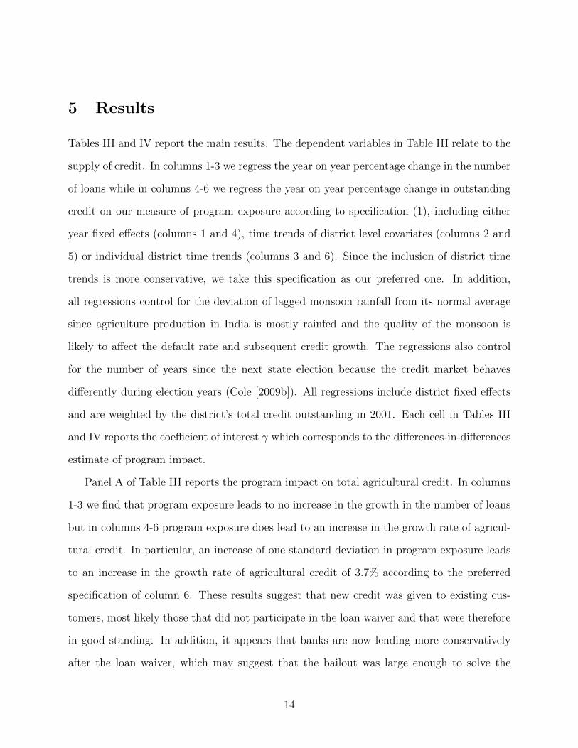
of 0.8%. Figure 4 complements TableV by plotting the coefficient estimates and the 90%
confidence intervals of amount dibursed (Figure 4a) and number of loans (Figure 4b). WHile
the point estimates on disbursement are positive and significant in 2009 and 2010, none of the
coefficients on the number of accounts are significantly different from zero. This corroborates
the fact that banks have improved lending practices by restricting the number of loans and
raising average loans among pre-existing borrowers in good standing.
Finally Tables VIII and IX explore the heterogeneity of impacts of the program. Table
VIII focuses on heterogeneity in district income. Our criterion for splitting the sample
into high and low-income districts is whether districts receive support from the Backward
Region Grant Fund Program (BRGF), a federal grant program targeted to the 250 poorest
districts in the country. Using our preferred specification in columns 3, 6 and 9 we find that
the effects of the program are concentrated in higher income districts, perhaps where the
growth opportunities were larger. Table IX focuses instead on the initial level of financial
development, proxied by the number of bank branches per capita in a district in the base
year 2001. Consistent with the findings of Table VIII, the program had greater impact in
districts with higher initial level of financial development.
6 Conclusion
Around the world, governments have routinely intervened in credit markets in an effort
to stimulate economic activity. Although it is often hypothesized that such interventions
have severe repercussions for credit discipline and borrower expectations, surprisingly little
robust evidence exists to evaluate these claims. In this paper, we use a natural experiment
surrounding one of the largest borrower bailouts in history to estimate the effect of a large
economic stimulus program on productivity and loan repayment.
17
We find that the program generated no measurable productivity gains, but led to sig-
nificant moral hazard in loan repayment. The annual post-program increase in the share of
non-performing loans grows up to 5 annual percentage points faster in districts in the highest
quintile of the debt relief distribution. Importantly, our findings also suggest a mechanism
for the amplification of moral hazard in loan repayment arising from economic stimulus en-
acted through the credit market. We show that the relationship between defaults and the
electoral cycle documented by earlier studies is magnified by the bailout program. This sug-
gests that the adverse effects of the bailout become more persistent as the stimulus generates
expectations of future politically motivated interventions in the credit market.
Taken together, these results provide some of the first evidence on the moral hazard gen-
erated by large government stimulus programs operating through the credit market. While
such programs have received much attention in the aftermath of the recent global financial
crisis, it is worth noting that programs of this kind, often more frequent and larger in scale,
have been carried out in many developing countries. Understanding the moral hazard conse-
quences of these large-scale economic stimulus programs is essential to weighing their costs
and benefits, particularly in an environment where weak institutions make such programs
susceptible to political capture and manipulation. The results in this paper are a first step
in this broader research agenda.
References
Agarwal, Sumit, G. Amromin, I. Ben David, S. Chomsisengphet, T. Piskorski,and A. Seru, “Policy Intervention in Debt Renegotiation: Evidence from the HomeAffordability Modification Program,” Working Paper, 2013.
Bolton, Patrick and H. Rosenthal, “Political Intervention in Debt Contracts,” Journalof Political Economy, 2002, 110 (5), 1103–1134.
Burgess, Robin and Rohini Pande, “Do Rural Banks Matter? Evidence from the IndianSocial Banking Experiment,” The American Economic Review, 2005, 95 (3), 780–795.
18

Campbell, John, S. Giglio, and P. Pathak, “Forced Sales and House Prices,” AmericanEconomic Review, 2011, 101 (5), 2108–2131.
Cole, Shawn A., “Financial Development, Bank Ownership, and Growth. Or, Does Quan-tity Imply Quality?,” The Review of Economics and Statistics, 2009, 91 (1), 33–51.
, “Fixing Market Failures or Fixing Elections? Elections, Banks and Agricultural Lendingin India,” American Economic Journals: Applied Economics, 2009, 1 (1), 219–250.
Diamond, Douglas W. and R. Rajan, “A Theory of Bank Capital,” Journal of Finance,2000, 55 (6), 2431–2465.
Gianetti, Mariassunta and Andrei Simonov, “On the Real Effects of Bank Bailouts:Micro Evidence from Japan,” American Economic Journal: Macroeconomics, 2013, 5 (1),135–167.
Guiso, Luigi, Paola Sapienza, and Luigi Zingales, “The Determinants of Attitudestoward Strategic Default on Mortgages,” Journal of Finance, 2013, 68 (4), 1473 – 1515.
Mian, Atif, Amir Sufi, and Francesco Trebbi, “Foreclosures, House Prices and theReal Economy,” American Economic Review, 2010, 100 (5), 1967–1998.
and , “The Effects of Fiscal Stimulus: Evidence from the 2009 Cash for ClunkersProgram,” Quarterly Journal of Economics, 2012, 127 (3), 1107–1142.
Paravisini, Daniel, “Local Bank Financial Constraints and Access to External Finance,”Journal of Finance, 2008, 63 (5).
Peek, Joseph and Eric S. Rosengren, “Unnatural Selection: Perverse Incentives andthe Misallocation of Credit in Japan,” American Economic Review, September 2005, 95(4), 1144–1166.
Philippon, Thomas and P. Schnabl, “Efficient Recapitalization,” Journal of Finance,2013, 68 (1), pp. 1–42.
Rucker, Randal and L. Alston, “Farm Failures and Government Intervention: A CaseStudy of the 1930s,” The American Economic Review, 1987, 77, 724–730.
Strahan, Philip E. and Jith Jayaratne, “The Finance-Growth Nexus: Evidence fromBank Branch Deregulation,” The Quarterly Journal of Economics, 1996, 111 (3).
19

Tables and Figures
Table I: Program Exposure
The table reports summary statistics for the variable ‘Bailout share’, our main measure of programexposure at the district level. The variable measures the total amount of credit eligible for the bailoutas a share of total outstanding agricultural credit at the district level, winsorized at the top percentile.Data on the total amount of debt relief granted is taken from the official figures of the respective StateLevel Bankers’ Committees, reported after the closing of the program in December 2011. Informationon the amount of credit eligible for the program was available for 491 districts, located in 22 ofIndia’s 28 states and 3 of 7 Union Territorries.The denominator of our measure of program exposure,total outstanding rural credit, is taken from the Reserve Bank of India’s Basic Statistical Returnsof Commercial Banks in India, and measures outstanding credit as of March 31, 2008. To facilitatethe interpretation of our estimates, we normalize the variable ‘Bailout share’ to have mean zero andstandard deviation one in all subsequent tables.
Bailout share
[N=491]
Mean .326
Median .284
StDev .224
Min .002
Max .991
20
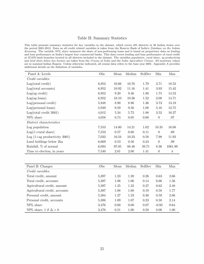
Table II: Summary Statistics
This table presents summary statistics for key variables in the dataset, which covers 491 districts in 28 Indian states overthe period 2001-2012. Data on all credit related variables is taken from the Reserve Bank of India’s Database on the IndianEconomy. The variable NPL share measures the share of non-performing loans and is based on proprietary data on lendingand loan performance at India’s largest four commercial banks. This data covers lending and loan performance of rural creditat 27,678 bank branches located in all districts included in the dataset. The variables population, rural share, ag productivityand land share below two hectare are taken from the Census of India and the India Agriculture Census. All monetary valuesare in nominal Indian Rupees. Unless otherwise indicated, all census data refers to the base year 2001. Appendix A providesadditional details on the definition of variables.
Panel A: Levels Obs Mean Median StdDev Min Max
Credit variables
Log(total credit) 6,952 10.66 10.76 1.79 3.71 18.52
Log(total accounts) 6,952 10.92 11.16 1.41 3.93 15.42
Log(ag credit) 6,952 9.20 9.46 1.80 1.75 14.52
Log(ag loans) 6,952 10.10 10.36 1.52 2.08 14.71
Log(personal credit) 5,948 8.90 8.90 1.36 3.73 13.19
Log(personal loans) 5,949 9.59 9.56 1.08 5.16 12.75
Log(total credit 2001) 4,012 5.34 5.72 1.88 3.52 16.27
NPL share 4,058 0.74 0.05 0.08 0 .97
District characteristics
Log population 7,553 14.00 14.21 1.02 10.35 16.08
Log(1+rural share) 7,553 0.57 0.60 0.11 0 .69
Log (1+ag productivity 2001) 7,033 10.24 10.23 0.58 7.98 11.92
Land holdings below 2ha 6,669 0.53 0.56 0.24 0 .99
Rainfall, % of normal 6,094 97.05 88.46 50.71 8.36 1061.99
Time to election, in years 7,540 2.01 2.00 1.41 0 4
Panel B: Changes Obs Mean Median StdDev Min Max
Credit variables
Total credit, amount 5,397 1.23 1.20 0.26 0.63 2.66
Total credit, accounts 5,397 1.06 1.06 0.14 0.66 1.56
Agricultural credit, amount 5,397 1.25 1.22 0.27 0.62 2.48
Agricultural credit, accounts 5,397 1.08 1.08 0.19 0.58 1.77
Personal credit, amount 5,384 1.27 1.23 0.30 0.59 2.66
Personal credit, accounts 5,386 1.09 1.07 0.23 0.58 2.14
NPL share 3,476 0.00 0.00 0.07 -0.93 0.64
NPL share, 1 if ∆ > 0 3,476 0.51 1.00 0.50 0.00 1.00
21
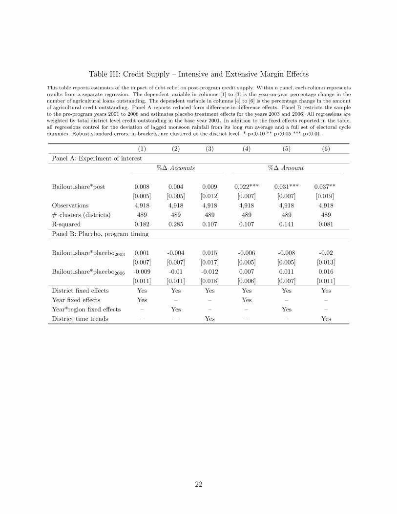
Table III: Credit Supply – Intensive and Extensive Margin Effects
This table reports estimates of the impact of debt relief on post-program credit supply. Within a panel, each column represents
results from a separate regression. The dependent variable in columns [1] to [3] is the year-on-year percentage change in the
number of agricultural loans outstanding. The dependent variable in columns [4] to [6] is the percentage change in the amount
of agricultural credit outstanding. Panel A reports reduced form difference-in-difference effects. Panel B restricts the sample
to the pre-program years 2001 to 2008 and estimates placebo treatment effects for the years 2003 and 2006. All regressions are
weighted by total district level credit outstanding in the base year 2001. In addition to the fixed effects reported in the table,
all regressions control for the deviation of lagged monsoon rainfall from its long run average and a full set of electoral cycle
dummies. Robust standard errors, in brackets, are clustered at the district level. * p<0.10 ** p<0.05 *** p<0.01.
(1) (2) (3) (4) (5) (6)
Panel A: Experiment of interest
%∆ Accounts %∆ Amount
Bailout share*post 0.008 0.004 0.009 0.022*** 0.031*** 0.037**
[0.005] [0.005] [0.012] [0.007] [0.007] [0.019]
Observations 4,918 4,918 4,918 4,918 4,918 4,918
# clusters (districts) 489 489 489 489 489 489
R-squared 0.182 0.285 0.107 0.107 0.141 0.081
Panel B: Placebo, program timing
Bailout share*placebo2003 0.001 -0.004 0.015 -0.006 -0.008 -0.02
[0.007] [0.007] [0.017] [0.005] [0.005] [0.013]
Bailout share*placebo2006 -0.009 -0.01 -0.012 0.007 0.011 0.016
[0.011] [0.011] [0.018] [0.006] [0.007] [0.011]
District fixed effects Yes Yes Yes Yes Yes Yes
Year fixed effects Yes – – Yes – –
Year*region fixed effects – Yes – – Yes –
District time trends – – Yes – – Yes
22

Table IV: Moral Hazard: Impact on Loan Performance
This table explores the impact of debt relief on post-program loan performance. The dependent variable in all regression is a
dummy equal to one for all years in which there an increase in the share of non-performing loans was recorded in a given district.
Columns [1] to [3] report difference-in-difference estimates for all districts in the sample. Columns [4] to [6] report coefficient
estimates for districts with greater than average bank competition, defined as districts in which the number of bank branches per
capita in the base year 2001 is greater than the sample mean. Data on loan performance are taken from a proprietary dataset
on loans and loan performance at India’s four largest public sector banks. The dataset covers loan performance at approximately
27,678 bank branches in 491 districts across 24 Indian states over the years 2006-2012. All regressions control for the deviation of
lagged monsoon rainfall from its long run average and years until the next state election. Robust standard errors, in brackets, are
clustered by district. * p<0.10 ** p<0.05 *** p<0.01.
(1) (2) (3) (4) (5) (6)
Panel A: Experiment of interest 1 if ∆ NPA share > 0
All districts High bank competition sample
Bailout share*post 0.074*** 0.088*** 0.080* 0.092*** 0.075** 0.240***
[0.021] [0.022] [0.048] [0.033] [0.033] [0.072]
Observations 2,676 2,676 2,676 1,402 1,402 1,402
# clusters (districts) 489 489 489 237 237 237
R-squared 0.243 0.276 0.297 0.214 0.253 0.305
Panel B: Placebo
Bailout share*placebo2007 -0.024 -0.027 -0.024 0.024 0.034 0.024
[0.036] [0.038] [0.036] [0.055] [0.060] [0.055]
District fixed effects Yes Yes Yes Yes Yes Yes
Year fixed effects Yes – – Yes – –
Year*region fixed effects – Yes – – Yes –
District time trends – – Yes – – Yes
23

Table V: Credit Supply and Loan Performance: Effects over Time
This table explores the impact of debt relief over time. The dependent variable in columns [1] and [2] are the change in
agricultural credit and the change in the number of agricultural loans outstanding. The dependent variable in colun [3] is
the share of non-performing l loans, as previously defined. The dependent variable in column [4] is agricultural productivity,
measured as the log revenue per hectare of all agricultural output in a district-year. All regressions control for the deviation
of lagged monsoon rainfall from its long run average and a full set of electoral cycle dummies. Robust standard errors, in
brackets, are clustered by district. * p<0.10 ** p<0.05 *** p<0.01.
(1) (2) (3) (4)
Dependent variable %∆ Ag credit %∆ NPL Productivity
Amount Loans 1 if >0
γt+1 0.061*** -0.007 0.087*** 0.001
[0.02] [0.01] [0.03] [0.00]
γt+2 0.031** -0.003 0.062** 0.008*
[0.01] [0.01] [0.03] [0.00]
γt+3 0.002 0.021** 0.104*** 0.005*
[0.01] [0.01] [0.03] [0.00]
Observations 4,918 4,926 2,682 4,241
#clusters (districts) 489 489 237 439
R-squared 0.142 0.287 0.28 0.181
Year fixed effects Yes Yes Yes Yes
Year*region fixed effects Yes Yes Yes Yes
District time trends – – – –
24

Table VI: Moral Hazard: Expectation of Future Bailouts
This table explores the interaction between post-program loan performance and the electoral cycle. The dependent variable in
all regressions is a dummy variable equal to one for district-year observations in which an increase in the share of non-performing
loans was recorded. Difference-in-difference estimates are obtained from a regression of this loan performance variable on the
interaction between the number of years to the next state election and a dummy variable equal to one for all post-program
observations and a set of time-varying controls. Columns [1] to [3] report estimates for the entire sample, columns [4] to [6]
report estimates for a ’high bank competition’ subsample, which includes only districts with a number of bank branches per
capita greater than the sample mean in the base year 2001. Data on loan performance are taken from a proprietary dataset on
loans and loan performance at India’s four largest banks. The dataset covers loan performance at approximately 27,678 bank
branches in 491 districts for the years 2006-2012. In addition to the fixed effects listed in the table, regressions control for the
deviation of lagged monsoon rainfall from its long run average and the number of years until the next state election. Robust
standard errors, in brackets, are clustered by district. * p<0.10 ** p<0.05 *** p<0.01.
(1) (2) (3) (4) (5) (6)
Panel A: Loan performance 1 if ∆ NPA share > 0
All districts High bank competition sample
Years to election*post -0.011 -0.035** -0.154*** -0.023 -0.051** -0.120***
[0.014] [0.017] [0.012] [0.021] [0.026] [0.017]
Observations 2,913 2,913 2,913 1,506 1,506 1,506
# clusters (districts) 508 508 508 237 237 237
R-squared 0.234 0.273 0.344 0.208 0.257 0.324
Panel B: Loan size Log loan size (district mean)
Years to election*post -0.002 -0.002 -0.006 0.001 0.006 -0.006
[0.006] [0.008] [0.005] [0.008] [0.011] [0.007]
Observations 2,406 2,406 2,406 1,244 1,244 1,244
# clusters (districts) 503 503 503 236 236 236
R-squared 0.444 0.471 0.736 0.485 0.526 0.752
District fixed effects Yes Yes Yes Yes Yes Yes
Year fixed effects Yes – – Yes – –
Year*region fixed effects – Yes – – Yes –
District time trends – – Yes – – Yes
25

Table VII: Impact on Productivity
This table explores the impact of debt relief on agricultural productivity. The dependent variable is the log per hectare revenue
from the sale of agricultural commodities at the district level. Columns [1] to [3] present unweighted difference-in-difference
estimates. Estimates in columns [4] to [6] are weighted by each district’s rural population share in the base year 2001. Data on
per hectare crop yields are taken from the Indian Department of Agriculture’s database on crop tields and revenue is calculated
using average commodity prices for the year 2001. Additional details on the calculation of the productivity series are reported
in Appendix C. Robust standard errors, in brackets, are clustered by district. * p<0.10 ** p<0.05 *** p<0.01.
(1) (2) (3) (4) (5) (6)
Log revenue per hectare
Bailout share*post 0.004 0.004 0.001 0.003 0.004* 0.001
[0.002] [0.003] [0.003] [0.002] [0.002] [0.002]
Observations 4,241 4,241 4,241 4,182 4,182 4,182
#clusters (districts) 488 488 488 488 488 488
R-squared 0.098 0.18 0.411 0.105 0.187 0.396
District fixed effects Yes Yes Yes Yes Yes Yes
Year fixed effects Yes – – Yes – –
Year*region fixed effects – Yes – – Yes –
District time trends – – Yes – – Yes
Weighted No No No Yes Yes Yes
26

Tab
leV
III:
Het
erog
eneo
us
Eff
ects
:D
istr
ict
Inco
me
in20
01
Th
eta
ble
rep
ort
sh
eter
ogen
eou
seff
ects
by
dis
tric
tle
vel
inco
me.
Dis
tric
tsare
class
ified
as
‘low
-in
com
e’if
the
rece
ived
fin
an
cial
sup
port
from
the
Back
ward
Reg
ion
sG
rant
Fu
nd
Pro
gra
m(B
RG
F),
ace
ntr
al
gover
nm
ent
pro
gra
mth
at
pro
vid
essu
pp
ort
for
dev
elop
men
tpro
ject
sin
the
poore
st250
dis
tric
tsof
Ind
ia.
Panel
Ap
rese
nts
esti
mate
sfo
rlo
w-i
nco
me
dis
tric
tsth
at
rece
ive
BR
GF
fun
din
g,
pan
elB
pre
sents
esti
mate
sfo
rh
igh
-in
com
ed
istr
icts
.W
ith
ina
pan
el,
each
colu
mn
rep
rese
nts
resu
lts
from
ase
para
tere
gre
ssio
n.
Th
edep
end
ent
vari
ab
lein
colu
mn
s[1
]to
[3]is
the
yea
r-on
-yea
rch
an
ge
into
talcr
edit
,an
dth
ed
epen
den
tvari
ab
lein
colu
mn
s[4
]to
[6]is
the
chan
ge
inou
tsta
nd
ing
loan
s.E
stim
ate
sin
colu
mn
s[1
]to
[6]
are
base
don
spec
ifica
tion
sid
enti
cal
toth
ose
inT
ab
leV
.T
he
dep
end
ent
vari
ab
lein
colu
mn
s[7
]to
[9]
isth
eyea
r-on
-yea
rch
an
ge
inn
on
-per
form
ing
loan
san
des
tim
ate
sare
base
don
spec
ifica
tion
sid
enti
cal
toth
ose
inT
ab
leV
I.A
llre
gre
ssio
ns
are
wei
ghte
dby
the
dis
tric
t’s
tota
lcr
edit
ou
tsta
nd
ing
in2001
an
dco
ntr
ol
for
the
dev
iati
on
of
lagged
mon
soon
rain
fall
from
its
lon
gru
naver
age,
an
dyea
rsu
nti
lth
en
ext
state
elec
tion
.R
ob
ust
stan
dard
erro
rs,
inb
rack
ets,
are
clu
ster
edat
the
dis
tric
tle
vel
.*
p<
0.1
0**
p<
0.0
5***
p<
0.0
1.
(1)
(2)
(3)
(4)
(5)
(6)
(7)
(8)
(9)
%∆
Loans
%∆
Amount
%∆
NPL
Panel
A:Low-IncomeDistricts
Bai
lou
tsh
are*
pos
t0.
016*
*0.
017*
*0.0
42**
0.0
47***
0.0
52***
-0.0
24
0.1
33***
0.1
44***
-0.0
39
[0.0
08]
[0.0
08]
[0.0
17]
[0.0
11]
[0.0
11]
[0.0
29]
[0.0
37]
[0.0
36]
[0.0
78]
Ob
serv
atio
ns
2,16
22,
162
2,1
62
2,1
62
2,1
62
2,1
62
1,1
40
1,1
40
1,1
40
R-s
qu
ared
0.23
10.
333
0.1
12
0.2
02
0.2
50.0
83
0.3
24
0.3
63
0.3
32
Panel
B:High-IncomeDistricts
Bai
lou
tsh
are*
pos
t0.
006
-0.0
020.0
37**
0.0
20**
0.0
22**
0.0
70***
0.0
51*
0.0
45
0.1
39**
[0.0
06]
[0.0
07]
[0.0
17]
[0.0
08]
[0.0
10]
[0.0
26]
[0.0
27]
[0.0
30]
[0.0
64]
Ob
serv
atio
ns
2,75
62,
756
2,7
56
2,7
56
2,7
56
2,7
56
1,5
36
1,5
36
1,5
36
R-s
qu
ared
0.16
10.
279
0.1
15
0.0
81
0.1
11
0.0
87
0.2
13
0.2
40.2
82
Dis
tric
tfi
xed
effec
tsY
esY
esY
esY
esY
esY
esY
esY
esY
esY
ear
fixed
effec
tsY
es–
–Y
es–
–Y
es–
–
Yea
r*re
gion
effec
ts–
Yes
––
Yes
––
Yes
–
Dis
tric
tti
me
tren
ds
––
Yes
––
Yes
––
Yes
27
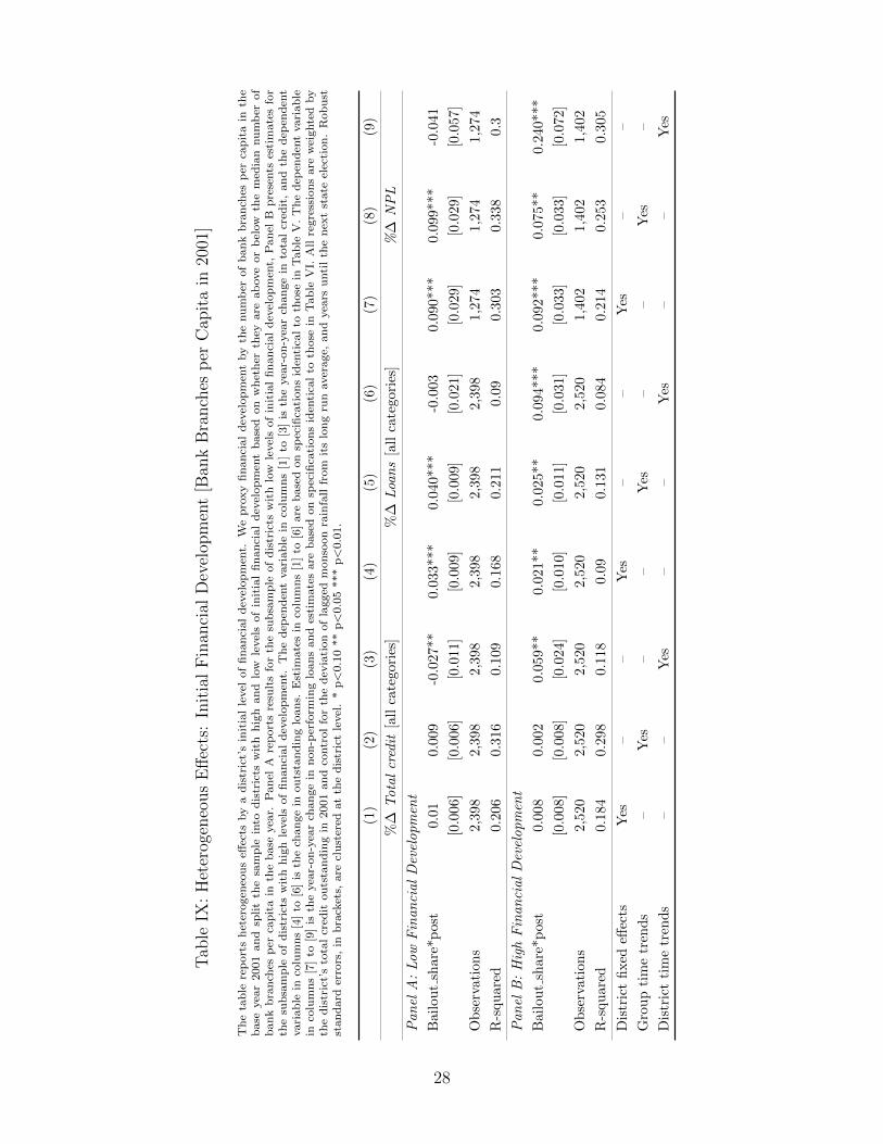
Tab
leIX
:H
eter
ogen
eous
Eff
ects
:In
itia
lF
inan
cial
Dev
elop
men
t[B
ank
Bra
nch
esp
erC
apit
ain
2001
]
Th
eta
ble
rep
ort
sh
eter
ogen
eou
seff
ects
by
ad
istr
ict’
sin
itia
lle
vel
of
fin
an
cial
dev
elop
men
t.W
ep
roxy
fin
an
cial
dev
elop
men
tby
the
nu
mb
erof
ban
kb
ran
ches
per
cap
ita
inth
eb
ase
yea
r2001
an
dsp
lit
the
sam
ple
into
dis
tric
tsw
ith
hig
han
dlo
wle
vel
sof
init
ial
fin
anci
al
dev
elop
men
tb
ase
don
wh
eth
erth
eyare
ab
ove
or
bel
ow
the
med
ian
nu
mb
erof
ban
kb
ran
ches
per
cap
ita
inth
eb
ase
yea
r.P
an
elA
rep
ort
sre
sult
sfo
rth
esu
bsa
mp
leof
dis
tric
tsw
ith
low
level
sof
init
ial
fin
an
cial
dev
elop
men
t,P
an
elB
pre
sents
esti
mate
sfo
rth
esu
bsa
mp
leof
dis
tric
tsw
ith
hig
hle
vel
sof
fin
an
cial
dev
elop
men
t.T
he
dep
end
ent
vari
ab
lein
colu
mn
s[1
]to
[3]
isth
eyea
r-on
-yea
rch
an
ge
into
tal
cred
it,
an
dth
ed
epen
den
tvari
ab
lein
colu
mn
s[4
]to
[6]
isth
ech
an
ge
inou
tsta
nd
ing
loan
s.E
stim
ate
sin
colu
mn
s[1
]to
[6]
are
base
don
spec
ifica
tion
sid
enti
cal
toth
ose
inT
ab
leV
.T
he
dep
end
ent
vari
ab
lein
colu
mn
s[7
]to
[9]
isth
eyea
r-on
-yea
rch
an
ge
inn
on
-per
form
ing
loan
san
des
tim
ate
sare
base
don
spec
ifica
tion
sid
enti
cal
toth
ose
inT
ab
leV
I.A
llre
gre
ssio
ns
are
wei
ghte
dby
the
dis
tric
t’s
tota
lcr
edit
ou
tsta
nd
ing
in2001
an
dco
ntr
ol
for
the
dev
iati
on
of
lagged
mon
soon
rain
fall
from
its
lon
gru
naver
age,
an
dyea
rsu
nti
lth
en
ext
state
elec
tion
.R
ob
ust
stan
dard
erro
rs,
inb
rack
ets,
are
clu
ster
edat
the
dis
tric
tle
vel
.*
p<
0.1
0**
p<
0.0
5***
p<
0.0
1.
(1)
(2)
(3)
(4)
(5)
(6)
(7)
(8)
(9)
%∆
Totalcredit
[all
cate
gori
es]
%∆
Loans
[all
cate
gori
es]
%∆
NPL
Panel
A:Low
FinancialDevelopmen
t
Bai
lou
tsh
are*
pos
t0.
010.
009
-0.0
27**
0.0
33***
0.0
40***
-0.0
03
0.0
90***
0.0
99***
-0.0
41
[0.0
06]
[0.0
06]
[0.0
11]
[0.0
09]
[0.0
09]
[0.0
21]
[0.0
29]
[0.0
29]
[0.0
57]
Ob
serv
atio
ns
2,39
82,
398
2,3
98
2,3
98
2,3
98
2,3
98
1,2
74
1,2
74
1,2
74
R-s
qu
ared
0.20
60.
316
0.1
09
0.1
68
0.2
11
0.0
90.3
03
0.3
38
0.3
Panel
B:HighFinancialDevelopmen
t
Bai
lou
tsh
are*
pos
t0.
008
0.002
0.0
59**
0.0
21**
0.0
25**
0.0
94***
0.0
92***
0.0
75**
0.2
40***
[0.0
08]
[0.0
08]
[0.0
24]
[0.0
10]
[0.0
11]
[0.0
31]
[0.0
33]
[0.0
33]
[0.0
72]
Ob
serv
atio
ns
2,52
02,
520
2,5
20
2,5
20
2,5
20
2,5
20
1,4
02
1,4
02
1,4
02
R-s
qu
ared
0.18
40.
298
0.1
18
0.0
90.1
31
0.0
84
0.2
14
0.2
53
0.3
05
Dis
tric
tfi
xed
effec
tsY
es–
–Y
es–
–Y
es–
–
Gro
up
tim
etr
end
s–
Yes
––
Yes
––
Yes
–
Dis
tric
tti
me
tren
ds
––
Yes
––
Yes
––
Yes
28
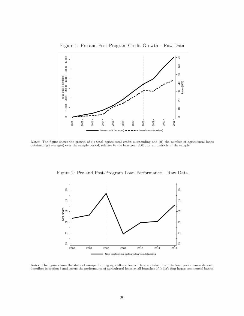
Figure 1: Pre and Post-Program Credit Growth – Raw Data
010
2030
4050
6070
Loan
s [’0
00]
010
0020
0030
0040
0050
0060
00To
tal c
redi
t [R
s m
illio
n]
2001
2002
2003
2004
2005
2006
2007
2008
2009
2010
2011
New credit (amount) New loans (number)
Notes: The figure shows the growth of (i) total agricultural credit outstanding and (ii) the number of agricultural loansoutstanding (averages) over the sample period, relative to the base year 2001, for all districts in the sample.
Figure 2: Pre and Post-Program Loan Performance – Raw Data.0
5.0
7.0
9.1
1.1
3.1
5
.05
.07
.09
.11
.13
.15
NPL
sha
re
2006 2007 2008 2009 2010 2011 2012
Non−performing ag loans/loans outstanding
Notes: The figure shows the share of non-performing agricultural loans. Data are taken from the loan performance dataset,describes in section 3 and covers the performance of agricultural loans at all branches of India’s four larges commercial banks.
29

Fig
ure
3:P
rogr
amE
xp
osure
and
Ex-P
ost
Loa
nP
erfo
rman
ce
(a)
Deb
tre
lief
[as
shar
eof
outs
tan
din
gcr
edit
]
q4 q3 q2 q1 No
data
(b)
∆N
PL
share
2009-2
012
q4 q3 q2 q1 No
data
No
tes:
Th
efi
gu
rep
lots
the
share
of
rura
lcr
edit
wri
tten
off
un
der
the
deb
tre
lief
pro
gra
min
Pan
el(a
)again
stin
crea
ses
inn
on
-per
form
ing
loan
sover
the
post
-pro
gra
m
per
iod
2009-2
011
inP
an
el(b
).T
he
share
of
cred
itw
ritt
enoff
un
der
the
pro
gra
mis
iden
tica
lto
the
trea
tmen
tvari
ab
led
escr
ibed
inT
ab
le1.
Incr
ease
sin
non
-per
form
ing
loan
sis
the
ari
thm
etic
mea
nof
the
an
nu
al
per
centa
ge
chan
ge
inth
esh
are
of
non-p
erfo
rmin
glo
an
s∆yt
=(y
t−
yt−
1)/yt−
1fo
rth
eyea
rs2009-2
011.
Loan
per
form
an
ce
isca
lcu
late
dfr
om
ap
rop
riet
ary
pan
eld
ata
on
rura
lcr
edit
an
dlo
an
per
form
an
eof
ind
ia’s
fou
rla
rges
tco
mm
erci
al
ban
ks
cover
ing
27,6
78
bra
nch
esin
all
dis
tric
tsin
the
data
set.
To
make
the
two
pan
els
com
para
ble
,P
an
el(b
)ex
clu
des
42
dis
tric
tsfo
rw
hic
hd
ata
on
deb
tre
lief
am
ou
nts
wer
en
ot
avail
ab
le.
30
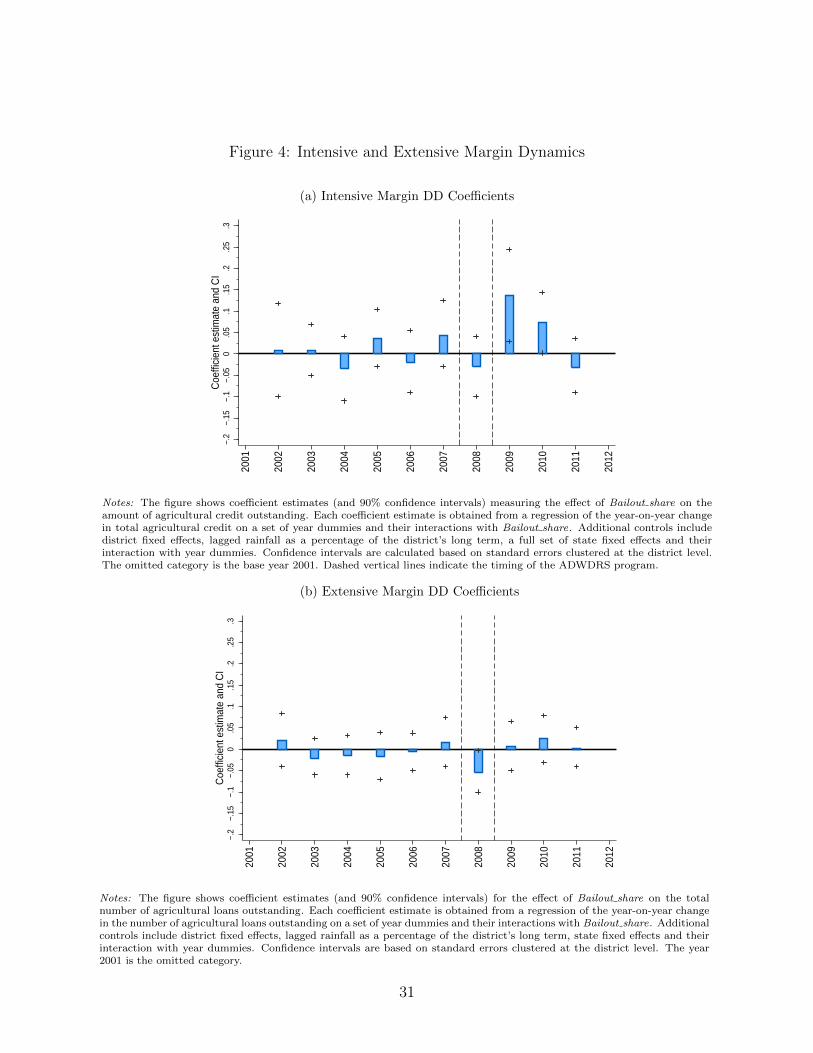
Figure 4: Intensive and Extensive Margin Dynamics
(a) Intensive Margin DD Coefficients
−.2
−.15
−.1
−.05
0.0
5.1
.15
.2.2
5.3
Coe
ffici
ent e
stim
ate
and
CI
2001
2002
2003
2004
2005
2006
2007
2008
2009
2010
2011
2012
Notes: The figure shows coefficient estimates (and 90% confidence intervals) measuring the effect of Bailout share on theamount of agricultural credit outstanding. Each coefficient estimate is obtained from a regression of the year-on-year changein total agricultural credit on a set of year dummies and their interactions with Bailout share. Additional controls includedistrict fixed effects, lagged rainfall as a percentage of the district’s long term, a full set of state fixed effects and theirinteraction with year dummies. Confidence intervals are calculated based on standard errors clustered at the district level.The omitted category is the base year 2001. Dashed vertical lines indicate the timing of the ADWDRS program.
(b) Extensive Margin DD Coefficients
−.2
−.15
−.1
−.05
0.0
5.1
.15
.2.2
5.3
Coe
ffici
ent e
stim
ate
and
CI
2001
2002
2003
2004
2005
2006
2007
2008
2009
2010
2011
2012
Notes: The figure shows coefficient estimates (and 90% confidence intervals) for the effect of Bailout share on the totalnumber of agricultural loans outstanding. Each coefficient estimate is obtained from a regression of the year-on-year changein the number of agricultural loans outstanding on a set of year dummies and their interactions with Bailout share. Additionalcontrols include district fixed effects, lagged rainfall as a percentage of the district’s long term, state fixed effects and theirinteraction with year dummies. Confidence intervals are based on standard errors clustered at the district level. The year2001 is the omitted category.
31

Appendix
Table A.I: Predicting Program Exposure
This table reports estimates from cross-sectional regressions of program exposure on measures of the land distribution and thetime series of weather shocks at the distric level. The dependent variable in all columns is the amount of debt relief as a shareof total outstanding agricultural credit at the time of the program. All regressions control for state fixed effects. Standard errorsare given in brackets and calculated using the Huber-White correction for heteroskedasticity. * p<0.10 ** p<0.05 *** p<0.01.
(1) (2) (3) (4) (5)
Bailout share
Share landholdings ≤ 2 ha -0.235*** -0.366 -0.366*** -0.571**
[0.086] [0.235] [0.099] [0.249]
Share landholdings > 2 ha 0.138 0.213
[0.227] [0.228]
Drought years2001−2007 0.029*** -0.044** -0.045**
[0.008] [0.020] [0.020]
Drought years*Landholdings ≤ 2 ha 0.131*** 0.133***
[0.032] [0.032]
Observations 4,607 4,607 5,056 4,607 4,607
Districts 491 491 491 491 491
R-squared 0.499 0.499 0.487 0.502 0.502
32

A Data Appendix
Table A.II: Description of Variables
Variable Description SourceTotal credit The natural logarithm (plus 1) of outstanding credit in units of Rs 100,000
for each district of India. Includes all loans given by private, public,cooperative and regional rural banks. Adjusted to account for loans belowRs 200,000 using district level loan size distributions reported in IndiaAgricultural Census Input Survey 2001.
Reserve Bank of India,Basic StatisticalReturns of ScheduledCommercial Banks inIndia, (2001 -2012)
Total credit,agriculture
The natural logarithm (plus 1) of total agricultural credit in units of Rs100,000 for each district of India. This includes direct agricultural financeand financing for activities related to agriculture and covers all loans givenby private, public, cooperative and regional rural banks. Adjusted toaccount for loans below Rs 200,000 using district level loan size distributionsreported in India Agricultural Census Input Survey 2001.
Reserve Bank of India,Basic StatisticalReturns of ScheduledCommercial Banks inIndia, (2001-2012)
Total personal credit The natural logarithm (plus 1) of total personal credit. This includes allcredit given by private, public, cooperative and regional rural banks. Itexcludes loans given for the purchase of durables and is adjusted for loansbelow Rs 200,000 using district level loan size distributions reported in IndiaAgriculture Census, Input Survey 2001.
Reserve Bank of India,Basic StatisticalReturns of ScheduledCommercial Banks inIndia, (2001-2012)
Non-performing loans This information is not publicly available. We have calculated it fromproprietary data obtained from four of India’s largest five banks. The dataconsists of annual information on the amount of outstanding rural creditand the amount of rural NPAs (both denominated in units of Rs 100,000).The dataset covers the period 2006-2012 and contains district levelaggregates of approximately 27,678 branches in all states and UnionTerritories of India (Reserve Bank of India, A Profile of Banks, 2012).
Proprietary bank data.
Rainfall Log deviation of monsoon rainfall (in mm) from its 50 year district-levelaverage. Monsoon rainfall is defined as total rainfall between June andSeptember. Long-run normals are taken from India MeteorologicalDepartment Long Run Averages of Climatological Normals, CD-ROM.
India MeteorologicalDepartment [IMD]
Electoral cycle Five dummy variables indicating the temporal distance to the nextscheduled state assembly election. State assembly elections are scheduledevery five years and are staggered over time.
Election Commissionof India, available athttp://eci.nic.in.
Total population, 2001Rural population, 2001
Total adult population and rural population of each district between theages of 15-65 years in 2001.
Census of India,District Tables (2001)
Total agriculturalproductivity
Per hectar value of output of 32 standard crops in units of Rs 1,000 at thedistrict level.
India AgricultureCensus, DistrictTables (2001)
Land distribution Share of landholdings in the district less than two hectares (approximately 5acres) in size.
India AgricultureCensus, DistrictTables (2001)
Drought AffectedDistrict
Dummy variable equal to one if a district was classified as ’drought affected’at the time that the debt relief program came into effect. The program hada higher minimum disbursement for qualifying households in these districts.
Reserve Bank of India
Low income district Dummy variable equal to one if a district receives subsidies from theBackward Regions Grant Fund (BRGF) program.
India Ministry ofStatistics and ProgramImplementation[MOSPI]
33

B Program Exposure by State
This section reports the share of total credit waived at the state level ordered by programexposure. Bailout share denotes the share of total agricultural credit outstanding waivedunder the program and includes both unconditional debt relief for households below the2 hectare program threshold and conditional debt relief for households above the programcutoff. The reported state level figures are the average figure for all districts in each stateincluded in our dataset.
Rank State Bailout share Rank State Bailout share
1. Orissa 60.2% 12. Sikkim 23.0%
2. Maharashtra 50.0% 13. Himachal Pradesh 22.7%
3. Jharkhand 41.3% 14. Chhattisgarh 22.0%
4. Tripura 39.4% 15. Rajasthan 21.4%
5. Andhra Pradesh 38.5% 16. Karnataka 16.8%
6. Bihar 37.7% 17. West Bengal 16.4%
7. Uttar Pradesh 31.8% 18. Jammu & Kashmir 13.8%
8. Uttaranchal 31.7% 19. Tamil Nadu 12.2%
9. Haryana 31.1% 20. Gujarat 11.1%
10. Madhya Pradesh 25.9% 21. Punjab 9.2%
11. Kerala 23.0% 22. Goa 2.2%
C District-Level Productivity
This section describes the construction of the productivity time series for each district,used in Table VII. To construct this variable, we use data on crop yields from the IndianDepartment of Agriculture (available at http://apy.dacnet.nic.in/). The dataset is anunbalanced panel which reports the (i) area cultivated and (ii) total harvest in tons for eachthe 25 most common crops in India for all districts of India over the time period 2000/01- 2010/11. We first aggregate these data to the district as defined in the 2001 census, ourunit of analysis throughout the paper. The for each year and crop we aggregate total areaplanted and crop output for both crop seasons (Kharif and Rabi). To measure productivityin monetary terms, we obtained commodity prices for the base year 2001 from Indiastat(District-wise Farm Harvest Prices of Principal Crops in India available at http://www.
indiastat.com/agriculture/) for all crops in the dataset as of January 2001. Letting acdydenote the area planted with crop c ∈ {1...C} in district d and year y, letting rcdy denotethe total production of crop c in district d and year y, and letting pc′01 denote the price ofcommodity c in the base year 2001, we calculate productivity per hectare in district d and
year y as Productivitydy =∑C
c=1{rcdy ·p
c‘01}∑C
c=1acdy
.
34