The Economic Impact of Social Ties:

Evidence from German Reunification∗

Konrad B. Burchardi† Tarek A. Hassan‡

November, 2010

Job Market Paper

Abstract

We use the fall of the Berlin Wall in 1989 to identify a causal effect of social ties betweenWest and East Germans on economic growth, household income, and firm investment: WestGerman regions which (for idiosyncratic reasons) had closer social ties to East Germanyprior to 1989 experienced faster growth in income per capita after reunification. A onestandard deviation rise in the share of households with social ties to East Germany isassociated with a 4.6% rise in income per capita over five years. Much of this effect onregional economic growth seems to be driven by a rise in entrepreneurial activity. Moreover,firms which are based in West German regions with closer social ties to the East in 1989 aremore likely to operate a subsidiary in East Germany even today. At the household level,West German households with relatives in East Germany in 1989 experienced a persistentrise in their income after the fall of the Berlin Wall. We interpret our findings as evidenceof a persistent effect of social ties in 1989 on regional economic development and provideevidence on possible mechanisms.

JEL Classification: O11, P16, N40.

Keywords: economic development, German reunification, networks, social ties.

∗We are grateful to Philippe Aghion, Oriana Bandiera, Tim Besley, Davide Cantoni, Wendy Carlin, JasonGarred, Maitreesh Ghatak, Claudia Goldin, Jennifer Hunt, Erik Hurst, Nathan Nunn, Rohini Pande, TorstenPersson, Michael Peters, Steve Redding, Daniel Sturm, and seminar participants at Harvard, the University ofChicago, UCLA, the London School of Economics, the EDP Meeting London, and London Business School foruseful comments. All mistakes remain our own.†London School of Economics and Political Science, STICERD, Houghton Street, London WC2A 2AE, United

Kingdom. E-mail: k.b.burchardi@lse.ac.uk.‡University of Chicago, Booth School of Business, 5807 South Woodlawn Avenue, Chicago IL 60630 USA;

E-mail: Tarek.Hassan@ChicagoBooth.edu.

1

1 Introduction

There are important theoretical reasons to believe that social ties between individuals impact eco-

nomic development. Social ties might facilitate communication and thereby reduce informational

frictions and asymmetries (Granovetter (1973), Varian (1990), Stiglitz (1990)). Furthermore, the

threat of severing social ties may serve as a form of ‘social’ collateral and thereby sustain a large

range of credit, insurance and trade contracts that would not otherwise be feasible (Besley and

Coate (1995)). Although both of these channels may fundamentally affect the ability of indi-

viduals to engage in economic transactions, there exists virtually no evidence to date on the

relevance of social ties for aggregate economic outcomes, such as economic growth and the scale

and success of entrepreneurial activity. In this paper we estimate the relevance of social ties

between individuals for regional economic development and trace the economic impact of social

ties to firm investment and household income.

The main obstacle to estimation of the causal effect of social ties on economic outcomes is

that social ties are endogenous to economic activity. At the microeconomic level, individuals may

form social ties in anticipation of future economic benefits, or as a result of economic interaction.

At the aggregate level, the regional distribution of social ties is a result of decisions of individuals

about where to live, and these decisions are endogenous to economic incentives. Identifying a

causal link between social ties and economic outcomes thus requires (i) the identification of ‘real

friends’, i.e. social ties that formed without regard to future economic benefits, and (ii) some

exogenous variation in the regional distribution of these exogenously formed social ties. In this

paper we use the fall of the Berlin Wall as a natural experiment, which enables us to overcome

both of these difficulties by exploiting two peculiar features of Germany’s post-war history. First,

the partition of Germany was generally believed to be permanent, so that individuals maintaining

social ties across the inner-German border must have done so for purely non-economic reasons.

Second, the pattern of wartime destruction in West Germany made it temporarily much more

difficult to settle in some parts of West Germany than in others, precisely during the period

during which millions of refugees and expellees from the East arrived in the West.

We find that West German regions which (for exogenous reasons) received a larger inflow

of expellees from East Germany before the construction of the Berlin Wall have significantly

stronger social ties to East Germany in 1989 and exhibit substantially higher growth in income

per capita after the fall of the Berlin Wall. This economic expansion is associated with a rise of

the returns to entrepreneurial activity and with an increase in the share of the population who

are entrepreneurs. Moreover, firms which are headquartered in West German regions which have

stronger social ties to East Germany in 1989 are more likely to operate a subsidiary or a branch

in eastern Germany today. In addition, West German households who have a relative in East

Germany in 1989 experience a persistent rise in personal income after the fall of the Berlin Wall.

1

The household level effects explain only around one sixth of the aggregate level effects, suggesting

strong spill-over effects. We interpret these findings as evidence of a causal link between social

ties and regional economic development in West Germany.

The first key advantage of the natural experiment surrounding German reunification is the

fact that the fall of the Berlin Wall was largely unexpected. After the physical separation of

the two German states in 1961, private economic exchange between the two Germanys was

impossible.1 Social ties that West Germans maintained with East Germans during this period

were then kept up for purely non-economic reasons, as individuals on both sides of the border

did not expect an economic re-integration. On November 9th 1989, these social ties suddenly

took on economic value: after the fall of the Berlin Wall, trade between the two Germanys

became feasible, following more than three decades of isolation. The result was a boom in

economic exchange between West and East.2 In this situation, East Germans had valuable local

information about demand conditions and about the quality of the assets that were offered to

investors. However, they were largely unable to borrow (indeed, until the mid-1990s many did

not know whether they owned their own homes) and lacked experience of the rules and norms

of behavior in a capitalist economy. West Germans, on the other hand, had these capacities

but lacked the requisite local knowledge. To the extent to which social ties facilitate economic

exchange, social ties between East and West Germans thus suddenly took on economic value on

the day of the fall of the Berlin Wall.

In our analysis we work with aggregate data on the share of individuals with social ties to East

Germany.3 This dataset shows that there was substantial variation in the share of individuals

with social ties to the East across West German regions. The second key advantage of the natural

experiment surrounding German reunification is that much of this variation has its roots in the

idiosyncrasies of Germany’s post-war history. Indeed, we show that West German regions which

received a large inflow of refugees and expellees from East Germany between 1945 and 1961

tend to have significantly stronger social ties to the East in 1989.4 However, the assignment of

refugees and expellees from the East to West German regions might not be random, as individuals

1In fact it had been highly restricted as far back as the late 1940s.2Moreover, almost the entire East German capital stock was sold to private investors between 1990 and 1994.

This boom was fueled by large transfers from West to East. These included both direct and indirect governmenttransfers. For example, the East German Mark was converted to the Deutsche Mark at several times its marketvalue. See (Sinn and Sinn, 1992, p. 51) and Lange and Pugh (1998), respectively.

3This measure of social ties thus captures bilateral ties. We are therefore not able to test network-theoreticalmodels of social ties.

4‘Refugees’ are individuals who in 1939 had their primary residence in the territory that became the Sovietsector post-World War II and who then fled to West Germany between 1945 and 1961.‘Expellees’ are individuals who in 1939 had their primary residence in areas of the German Reich which becamepart of Poland, Russia or another country from which ethnic Germans were expelled post-World War II. We focuson the group of expellees who held a residence in the Soviet sector after the war, but migrated to West Germanybetween 1945 and 1961 (as did the vast majority of expellees who were originally allocated to the Soviet sector).

2

may have moved to those regions in which they saw the best prospects for themselves and their

families. In particular, an overwhelming concern for those arriving from the East after 1945

was the acute housing crisis in West Germany, which persisted until the early 1960s. This crisis

resulted from the fact that during World War II, 32% of the West German housing stock was

destroyed. The expellees and refugees arriving from the East were thus channeled predominantly

into areas in which there was relatively more intact housing, i.e. to the areas that were least

destroyed during the war.

Variation in wartime destruction which temporarily made it more difficult to settle in some

parts of West Germany than in others thus provides the exogenous source of variation in the

regional distribution of social ties which we need in order to identify a causal effect of social ties

on regional economic outcomes. In particular, we use the degree of wartime destruction in 1945

as an instrument for the share of expellees settling in a given West German region. The main

identifying assumption for our region-level results is thus that the degree of wartime destruction

in 1945 (or any omitted factors driving it) affected growth in income per capita after 1989 only

through the settlement of refugees and expellees post World War II; and that these groups indeed

affect growth post-1989 exclusively due to their social ties to East Germany.

We devote a great deal of care to corroborating this identifying assumption in various ways.

For example, we show that wartime destruction is uncorrelated with pre-war population growth,

that it affects post-war population growth only until the 1960s, and that it has no effect on the

growth of income per capita in West German regions in the years before 1989. Moreover, all of

our specifications are robust to controlling for the growth in income per capita in the years prior

to 1989. Finally, we show that our results are particular to expellees arriving from East Germany

rather than to other expellees who arrived directly to West Germany, i.e. without settling in

East Germany for some time.

Based on this identifying assumption, we show a strong causal relationship between the

intensity of social ties to East Germany and post-1989 growth in income per capita among West

German regions: a one standard deviation rise in the share of expellees from East Germany

settling in a given West German region in 1961 is associated with a 4.6% rise in income per

capita over the six years between 1989 and 1995. This is a sizable effect, amounting to around

0.7 percentage points higher growth per year.5 While the regional growth effect diminishes after

1995, there is no evidence of a subsequent reversal, so that the pattern of social ties to the

East which existed in 1989 may have permanently altered the distribution of income across West

German regions.

In an effort to shed light on the mechanism linking social ties to regional economic growth

5This result is robust to several different variations in the estimation strategy and cannot be explained bylikely alternatives, such as migration from East to West in 1989 or by a decline in West German heavy industryin the 1990s.

3

we estimate separate effects for the incomes of entrepreneurs and non-entrepreneurs. While

both entrepreneurs and non-entrepreneurs who live in regions with strong social ties to the East

experience a significant rise in their incomes, the incomes of entrepreneurs increase at more than

twice the rate of those of non-entrepreneurs. Consistent with this observation, the share of the

population engaged in entrepreneurial activity rises in regions with strong social ties.

To trace this effect of social ties on entrepreneurial activity to the behavior of firms, we use

data on the cross-section of West German firms in 2007. We show that West German firms which

are headquartered in a region which had strong social ties to the East in 1989 are more likely

to operate a subsidiary or a branch in East Germany in 2007. In particular, a one standard

deviation rise in the share of expellees from East Germany settling in a region before 1961 is

associated with a 3.4% increase in the likelihood that a given firm within that region operates a

subsidiary or branch in East Germany in 2007. Interestingly, this effect seems to be concentrated

in the services sector, which is consistent with the view that social ties are particularly important

in industries which rely heavily on local information. While social ties to East Germany predict

a higher probability of investing in East Germany, they do not predict a higher probability of

investing anywhere else in the world, except for a small rise in the probability of investing in

Poland. This latter finding is notable as many of those arriving in West Germany from East

Germany before 1961 were originally expelled from present-day Poland in 1945, then lived in

East Germany for up to 16 years and arrived in the West before the construction of the Berlin

Wall in 1961.

We then estimate the effect of social ties at the household level. We show that West German

households who report having relatives in East Germany in 1989 experience a persistent rise

in their income after the fall of the Berlin Wall: the income of households with at least one

relative in the East rises on average by 4.9% over the six years following the fall of the Berlin

Wall. This rise in income again occurs immediately after 1989 and is robust to controlling for

possible omitted variables, such as the age, level of education, or capital income of the household

head. Especially households headed by individuals below the age of 40 (lowest quartile of the

age distribution) and above the age of 52 (top two quartiles) seem to profit from their social

ties to East Germany. We also show that households profit from their ties to East German

relatives regardless of their level of capital income in 1989, which is consistent with the view

that households used their ties to the East primarily as conduits for information, rather than to

facilitate borrowing.

We interpret our results as evidence that social ties to East Germany indeed took on significant

economic value after the fall of the Berlin Wall: West Germans who had ties to the East were

better able to take advantage of the new economic opportunities in the East, possibly because

they were better informed about investment opportunities than their peers. The rise in regional

4

income seems to be driven primarily by an increase in entrepreneurial activity and by an increase

in the number of entrepreneurs. Moreover, firms which had access to a workforce with strong

social ties seem to have had a comparative advantage in investing in the East. Comparing the

quantitative implications of our household-level and our region-level results suggests that there

were significant spill-overs, through which households living in regions with strong ties to the

East experience rising incomes, even if they themselves do not have direct personal ties to the

East.

While we believe that this paper convincingly demonstrates the relevance of social ties for

regional economic development, there are two important caveats to the interpretation of our

results. First, it is unclear how our results generalize beyond the context of a large economic

transition, such as the economic re-integration of Germany. Social ties may be particularly useful

in an environment in which markets are established rapidly and informational asymmetries are

large. Second, we cannot be sure whether social ties led to an increase of economic activity at

the country level or whether they merely resulted in a re-distribution of rents from regions with

weaker social ties to regions with stronger social ties. However, the fact that we find positive

spill-overs rather than crowding out at the regional level suggests that Germany as a whole

was better off for its access to individuals with social ties.6 Finally, some of the patterns that

we document may be explained if there remain unobserved cultural differences in 1989 between

‘native’ West Germans and the population of expellees and refugees who settled in West Germany

post-World War II. We do not emphasize this interpretation, as Germans of all parts were fairly

homogenous before the separation, sharing a common language and culture. The integration

of the new arrivals into West German society is commonly regarded as one of the preeminent

achievements of post-war Germany, such that people would typically not know (or care) whether

their neighbors were descendants of expellees or refugees after the war.

To our knowledge, this paper is the first to identify the effect of social ties on aggregate eco-

nomic outcomes and the first to trace this effect from the households and firms to regional

economic development. Our results relate to a large literature which links social networks

and social ties to a broad set of microeconomic outcomes, ranging from employment (Mun-

shi (2003), Laschever (2007), and Beaman (2008)) and informal insurance (e.g. Weerdt and

Dercon (2006)) to performance in the financial industry (Cohen, Frazzini, and Malloy (2008),

Hochberg, Ljungqvist, and Lu (2007), and Kuhnen (2009)) and agricultural yields (Conley and

Udry (2009)). Since social ties have been documented to influence such a wide range of microe-

conomic outcomes, an obvious question to ask is whether they also influence aggregate economic

variables. While there are number of models that predict such aggregate effects (e.g. Rauch

6In the main part of the paper we only estimate the effects for West German districts - mainly due to a lackof East German data before 1989. If some of the surplus generated by social ties accrued to East Germans, ourestimates likely underestimate the total growth effect of social ties.

5

(1996), Rauch and Casella (1998), Kranton and Minehart (2001), and Ambrus, Mobius, and

Szeidl (2010)), we believe our paper to be the first to provide causally interpretable evidence on

this matter.

Most closely related to our empirical work is the paper by Fuchs-Schundeln and Schundeln

(2005) who use the reunification of Germany to identify the role of risk aversion in occupational

choice. A number of other authors have used the partition of Germany as natural experiment.

Redding and Sturm (2008) estimate the effect of market access on city growth, Alesina and

Fuchs-Schundeln (2007) estimate the effect of the East German regime on voter preferences, and

Bursztyn and Cantoni (2009) estimate the effect of exposure to West German media on consumer

preferences.

In using the effect of wartime destruction on the settlement of expellees in West Germany, we

also relate to a number of papers which quantify the effect of wartime destruction on long-run

economic development. At the aggregate level, Brakman, Garretsen, and Schramm (2004) find

that the pattern of wartime destruction had no long-run impact on city growth in West Germany.

Davis and Weinstein (2002) and Miguel and Roland (2006) show similar results for Japan and

Vietnam, respectively. At the individual level, Akbulut-Yuksel (2009) documents a detrimental

effect of wartime destruction on the education and health of school-age children who grew up in

the most affected areas.

The remainder of the paper is organized as follows: Section 2 reviews the historical back-

ground of wartime destruction, the partition of Germany, and the settlement of expellees and

refugees in West Germany. Section 3 discusses the data and its construction. Section 4 estab-

lishes the basic relationship between wartime destruction and social ties to the East, and uses

this relationship to identify a causal effect of social ties on growth in income per capita post-1989.

Section 5 provides evidence which suggests that entrepreneurial income and activity being the

main driver of aggregate income growth. In particular, section 5.2 documents the influence of

social ties on the ownership structure of German firms today. Section 6 looks at the relation-

ship between social ties and income growth at the household level. Section 7 discusses possible

mechanisms by which social ties might affect economic activity. Section 8 discusses our results,

while the appendix contains additional robustness checks and details on the construction of our

dataset.

2 Historical Background

2.1 Destruction of Housing Stock during World War II

German cities and towns were heavily destroyed after World War II. This was mainly the result

of Allied air raids, which began in 1940 and intensified until the final days of the war in 1945.

6

These left around 500,000 dead and resulted in the destruction of a third of the West German

housing stock, making it the most devastating episode of air warfare in history.7

In the early days of the war the Royal Air Force attempted to slow down the advance of the

German army into the Soviet Union by destroying transport infrastructure. This strategy was

an abject failure and was quickly abandoned, as the available technology at the time did not

permit targeted raids. At best, the pilots flying the nighttime raids were able to make out that

they were above a city (and they were often even unsure which city lay below). This led to the

adoption of the doctrines of ‘moral bombing’ (1941) and of ‘fire and carpet bombing’, which were

aimed at destroying the Germans’ morale and ability to resist by destroying cities and towns

(Kurowski (1977)). By the end of the war, 50% of the 900,000 metric tons of bombs deployed

had hit settlements, while 17% had hit industry or infrastructure.

The cities destroyed most during the early years of the war were those that were close to the

British shore and easy to spot from the air, e.g. Hamburg and Cologne. After 1944, utilizing

recent technological advances, the allies were able to implement fire storms, which were easiest

to create in cities with highly flammable, historical centers, such as Darmstadt, Dresden, or

Wuerzburg. Fire storms could typically not be implemented in cities which had already been hit

by a large number of explosive bombs, as the rubble from earlier raids would have prevented the

fire from spreading. This is why the cities that were attacked relatively late in the war (often

strategically the least important) were among the most heavily destroyed.8

Appendix Figure 1 shows the varying intensity of destruction in West German regions. Note

that none of our empirical results rely on this pattern being random or driven by certain factors.

Instead, our identification strategy relies on the assumption that the pattern of wartime destruc-

tion or any omitted factors driving it have no direct effect on growth in West German regions

45 years later, post 1989.

2.2 The Partition and Reunification of Germany

In 1944, as World War II entered its final phase, the UK, the US and the Soviet Union agreed

on a protocol for the partition of pre-war Germany: The areas to the east of the rivers Oder

and Neisse were to be annexed by Poland and by the Soviet Union, and the remaining territory

was to be divided into three sectors of roughly equal population. The UK would occupy the

Northwest, the US the South, and the Soviet Union the East. The capital, Berlin, would be

jointly occupied. At the end of the war, the three armies took control of their sectors, and the

7The information presented in this section is from U.S. Govt. Print Office (1945), Kurowski (1977), andFriedrich (2002).

8During a fire storm, a large section of a city catches fire, creating winds of up to 75 meters per second,depriving those exposed of oxygen and often sucking them into the fire.

7

US and Britain carved a small French sector out of their territory.9 In 1949, with the onset of the

Cold War, the three Western sectors formed the Federal Republic of Germany (West Germany),

and the Soviet sector became the German Democratic Republic (East Germany). Economic

exchange between the two parts of Germany became increasingly difficult as the East German

government immediately introduced central planning. Only three years later, in 1952, the border

was completely sealed, cutting any remaining legal or illegal trade links between East and West.10

Until the construction of the Berlin Wall in August 1961 there remained the possibility of

personal transit from East to West Berlin, which was the last remaining outlet for refugees fleeing

from East to West Germany. After 1961, migration between East and West virtually ceased. In

the following years the partition of Germany was formally recognized in various international

treaties, and was, until the summer of 1989, generally believed to be permanent.11

In September of 1989 it became apparent that a critical mass of East Germans had become

alienated from the socialist state, its declining economic performance, and the restrictions it

placed on personal freedom. Increasingly large public demonstrations led to the opening of the

Berlin Wall on November 9th, 1989. The first free elections in East Germany were held in March

of 1990, followed by the rapid political, monetary, and economic union between East and West

Germany by the end of the same year.

2.3 Refugees and Expellees in Western Germany, 1945-1961

In 1945 the Polish and Soviet authorities expelled all German nationals from the annexed ter-

ritory, so that areas which used to be German before 1939 could be inhabited by Polish (and

Russian) nationals after 1945. While many Germans in these regions had fled the advancing

Soviet Army, those that remained were marched or transported out of the annexed territories

towards the four sectors. We refer to this group of people as ‘expellees’. Germans that either

originally lived in or moved to the countries occupied by the German army during war were also

expelled in many cases, particularly from Czechoslovakia, Hungary, Romania, and Yugoslavia.

Expellees were registered and then assigned one of the four sectors in which to settle, according

to quotas fixed in the Potsdam accord.12 The authorities in turn allocated the expellees to the

9This entailed a significant withdrawal of the British and US forces, who had captured much more territorythan expected (Sharp (1975)).

10The only remaining trade between the two countries was the ‘Interzonenhandel’ which was arranged betweenthe two governments. In this system the East German government would trade goods and services by the bartersystem. In 1960 its total volume came to the equivalent of $178 m. See Holbik and Myers (1964) for a detaileddescription of the Interzonenhandel.

11The most important of these treaties was the ‘Grundlagenvertrag’ of December 1972 between East and WestGermany in which both countries recognized ‘two German states in one German nation.’ Following this treatyEast and West Germany were accepted as full members of the United Nations.

12The official plan adopted by the allies in November 1945 was to expel 6.65 million Germans. 2.75 million,were to be allocated to the Soviet sector and 2.25 million, 1.5 million, and 0.15 million to the American, British,

8

(later to become federal) states within their jurisdictions and assigned them quarters wherever

they could find intact housing stock.

The first wave of 5.96 million expellees arrived in the three Western sectors by 1946. We

refer to this group as ‘direct expellees’. As it became increasingly apparent that the division of

Germany would become permanent, most of the 3.04 million that had originally been allocated

to the Soviet sector left for the West. These ‘expellees via the Soviet sector’ are critical to

our empirical analysis as they had the opportunity to form social ties to East Germans before

migrating on to West Germany. By 1960, the total number of expellees in West Germany had

risen to 9.697 million, of which roughly one third were expellees via the Soviet sector.13

In parallel, an increasing number of native residents of the Soviet sector who were dissatisfied

with the political and economic prospects of the fledging East Germany fled to the West. This

flow of ‘refugees’ peaked in the years before the construction of the Berlin Wall, with on average

around 300,000 individuals illegally crossing the Border in each year between 1957 and 1961

(Hunt (2006)). By 1961 the total number of East German refugees settling in West Germany

was 3.5 million.

While the authorities in the western sectors, and later the West German authorities, had an

explicit policy supporting expellees, supplying them with housing and various subsidies, there

was very little support for refugees. In fact, as late as 1950 the authorities actively tried to

discourage refugees from entering West Germany on the grounds that they would exasperate an

already catastrophic situation in the housing market and for fear of the political consequences

of a de-populating East Germany. In practice, however, the authorities never attempted to

deport refugees back to the East, and so refugees often made their own way in West Germany,

without registering with the authorities.14 The severe housing crises that resulted from the

inflow of millions of migrants into the heavily destroyed Western sectors remained the principal

determinant in the allocation of expellees and refugees to West German cities and towns until

the late 1950s.15

and French sectors, respectively (Bethlehem (1982), p.29).13We are unable to determine exactly how many expellees remained in East Germany, as the communist

government declared after 1950 that the expellees had been fully integrated into East German society and bannedthe concept from subsequent government statistics (Franzen (2001)).

14See Bethlehem (1982, chapter 3).15In the early years the availability of housing was the only determinant of where the expellees were sent

(Bethlehem, 1982, p. 29, pp.49). After 1949 economic considerations started playing a more important role in theallocation process and the West German government also initiated a number of programs encouraging migrationto areas in which there was a relatively higher demand for labor. However, these programs remained relativelylimited, with less than one in ten expellees participating in them.

9

3 The Data

We use data at the household, firm, district (Landkreis), and regional (Raumordnungseinheit)

level. Districts are the equivalent of US counties. Regions are the union of several districts,

and each district belongs to one such unit. Regions do not have a political function but exist

exclusively for statistical purposes; in this sense they are analogous to metropolitan statistical

areas in the US, but also encompass rural areas. All of our aggregate data is available at the

district level, except for income per capita before 1995, which is available only at the regional

level. Our primary units of analysis are thus the 74 West German regions. When we use

aggregate controls in our firm and household level analysis we always use data at the lowest level

of aggregation available.

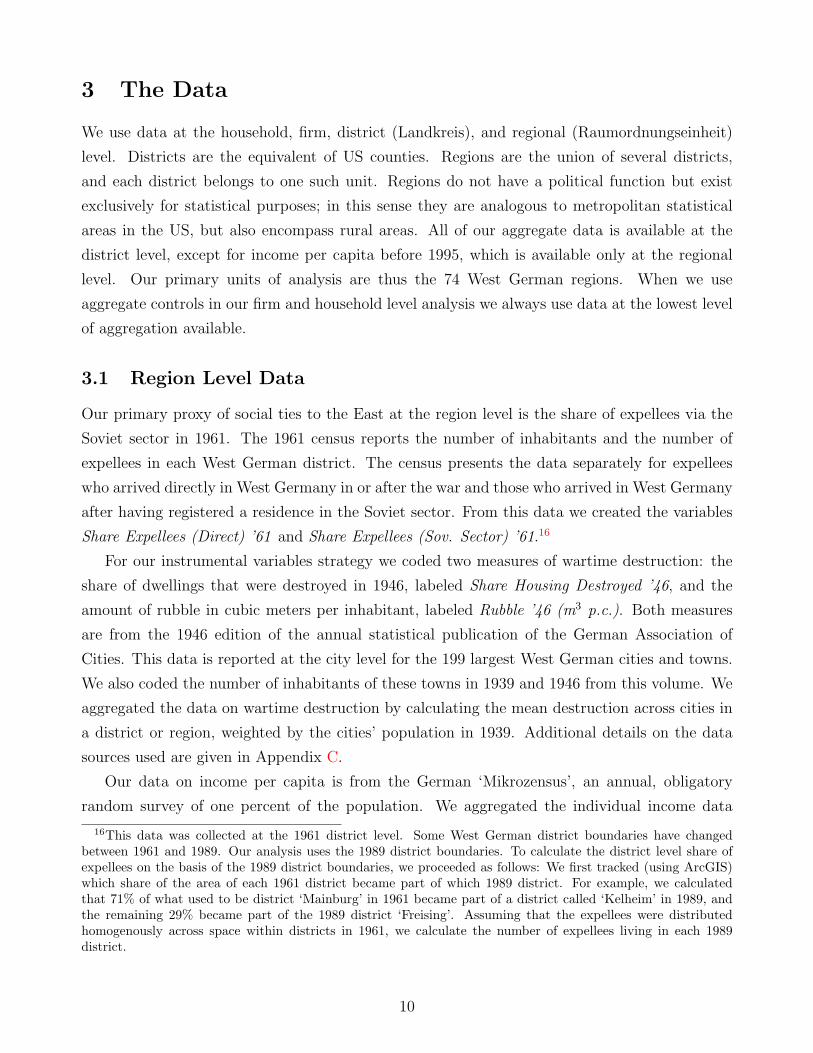
3.1 Region Level Data

Our primary proxy of social ties to the East at the region level is the share of expellees via the

Soviet sector in 1961. The 1961 census reports the number of inhabitants and the number of

expellees in each West German district. The census presents the data separately for expellees

who arrived directly in West Germany in or after the war and those who arrived in West Germany

after having registered a residence in the Soviet sector. From this data we created the variables

Share Expellees (Direct) ’61 and Share Expellees (Sov. Sector) ’61.16

For our instrumental variables strategy we coded two measures of wartime destruction: the

share of dwellings that were destroyed in 1946, labeled Share Housing Destroyed ’46, and the

amount of rubble in cubic meters per inhabitant, labeled Rubble ’46 (m3 p.c.). Both measures

are from the 1946 edition of the annual statistical publication of the German Association of

Cities. This data is reported at the city level for the 199 largest West German cities and towns.

We also coded the number of inhabitants of these towns in 1939 and 1946 from this volume. We

aggregated the data on wartime destruction by calculating the mean destruction across cities in

a district or region, weighted by the cities’ population in 1939. Additional details on the data

sources used are given in Appendix C.

Our data on income per capita is from the German ‘Mikrozensus’, an annual, obligatory

random survey of one percent of the population. We aggregated the individual income data

16This data was collected at the 1961 district level. Some West German district boundaries have changedbetween 1961 and 1989. Our analysis uses the 1989 district boundaries. To calculate the district level share ofexpellees on the basis of the 1989 district boundaries, we proceeded as follows: We first tracked (using ArcGIS)which share of the area of each 1961 district became part of which 1989 district. For example, we calculatedthat 71% of what used to be district ‘Mainburg’ in 1961 became part of a district called ‘Kelheim’ in 1989, andthe remaining 29% became part of the 1989 district ‘Freising’. Assuming that the expellees were distributedhomogenously across space within districts in 1961, we calculate the number of expellees living in each 1989district.

10

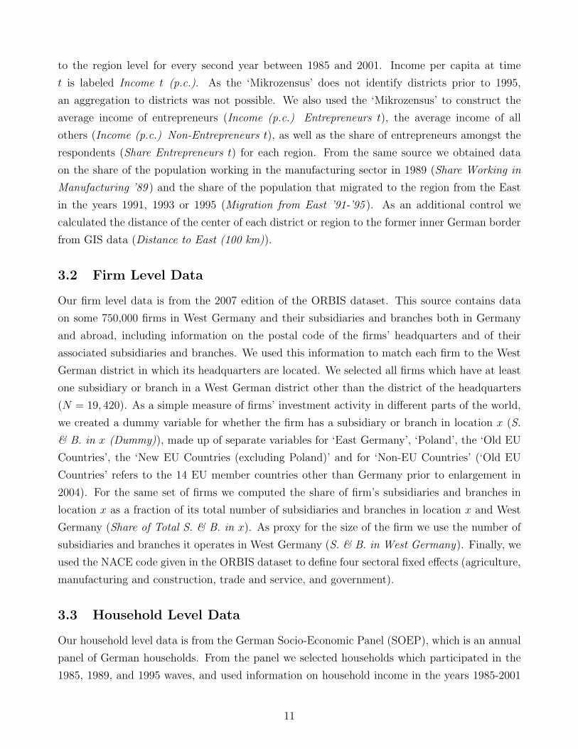
to the region level for every second year between 1985 and 2001. Income per capita at time

t is labeled Income t (p.c.). As the ‘Mikrozensus’ does not identify districts prior to 1995,

an aggregation to districts was not possible. We also used the ‘Mikrozensus’ to construct the

average income of entrepreneurs (Income (p.c.) Entrepreneurs t), the average income of all

others (Income (p.c.) Non-Entrepreneurs t), as well as the share of entrepreneurs amongst the

respondents (Share Entrepreneurs t) for each region. From the same source we obtained data

on the share of the population working in the manufacturing sector in 1989 (Share Working in

Manufacturing ’89 ) and the share of the population that migrated to the region from the East

in the years 1991, 1993 or 1995 (Migration from East ’91-’95 ). As an additional control we

calculated the distance of the center of each district or region to the former inner German border

from GIS data (Distance to East (100 km)).

3.2 Firm Level Data

Our firm level data is from the 2007 edition of the ORBIS dataset. This source contains data

on some 750,000 firms in West Germany and their subsidiaries and branches both in Germany

and abroad, including information on the postal code of the firms’ headquarters and of their

associated subsidiaries and branches. We used this information to match each firm to the West

German district in which its headquarters are located. We selected all firms which have at least

one subsidiary or branch in a West German district other than the district of the headquarters

(N = 19, 420). As a simple measure of firms’ investment activity in different parts of the world,

we created a dummy variable for whether the firm has a subsidiary or branch in location x (S.

& B. in x (Dummy)), made up of separate variables for ‘East Germany’, ‘Poland’, the ‘Old EU

Countries’, the ‘New EU Countries (excluding Poland)’ and for ‘Non-EU Countries’ (‘Old EU

Countries’ refers to the 14 EU member countries other than Germany prior to enlargement in

2004). For the same set of firms we computed the share of firm’s subsidiaries and branches in

location x as a fraction of its total number of subsidiaries and branches in location x and West

Germany (Share of Total S. & B. in x). As proxy for the size of the firm we use the number of

subsidiaries and branches it operates in West Germany (S. & B. in West Germany). Finally, we

used the NACE code given in the ORBIS dataset to define four sectoral fixed effects (agriculture,

manufacturing and construction, trade and service, and government).

3.3 Household Level Data

Our household level data is from the German Socio-Economic Panel (SOEP), which is an annual

panel of German households. From the panel we selected households which participated in the

1985, 1989, and 1995 waves, and used information on household income in the years 1985-2001

11

(Income (SOEP)), the amount of capital income in 1989, and the age and years of education

(including professional education) of the household head. We also created dummies for the

primary occupation and gender of the household head.17

Importantly, the SOEP questionnaire asked in 1991 whether the respondent had any relatives

in the other part of Germany. From this information we constructed our measure of social ties

at the household level (Ties to Relatives ’91 ), which is a dummy variable equal to 1 if at least

one individual in the household had a relative in the other part of Germany. We also aggregated

this variable to the region level by calculating the share of households with ties to East Germany

in each West German region (Share Ties to Relatives ’91 ), which we use as a secondary measure

of social ties. Lastly, we created a dummy variable indicating households whose household head

was an entrepreneur in 1989 (Entrepreneur ’89 ).

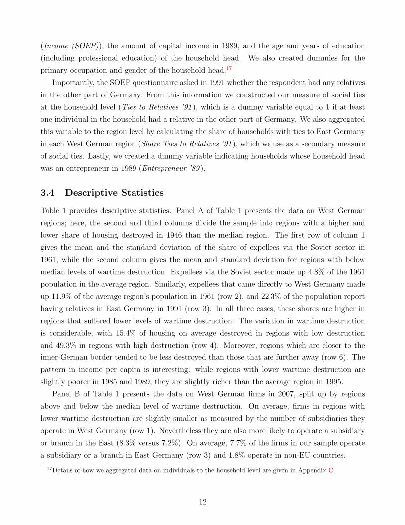
3.4 Descriptive Statistics

Table 1 provides descriptive statistics. Panel A of Table 1 presents the data on West German

regions; here, the second and third columns divide the sample into regions with a higher and

lower share of housing destroyed in 1946 than the median region. The first row of column 1

gives the mean and the standard deviation of the share of expellees via the Soviet sector in

1961, while the second column gives the mean and standard deviation for regions with below

median levels of wartime destruction. Expellees via the Soviet sector made up 4.8% of the 1961

population in the average region. Similarly, expellees that came directly to West Germany made

up 11.9% of the average region’s population in 1961 (row 2), and 22.3% of the population report

having relatives in East Germany in 1991 (row 3). In all three cases, these shares are higher in

regions that suffered lower levels of wartime destruction. The variation in wartime destruction

is considerable, with 15.4% of housing on average destroyed in regions with low destruction

and 49.3% in regions with high destruction (row 4). Moreover, regions which are closer to the

inner-German border tended to be less destroyed than those that are further away (row 6). The

pattern in income per capita is interesting: while regions with lower wartime destruction are

slightly poorer in 1985 and 1989, they are slightly richer than the average region in 1995.

Panel B of Table 1 presents the data on West German firms in 2007, split up by regions

above and below the median level of wartime destruction. On average, firms in regions with

lower wartime destruction are slightly smaller as measured by the number of subsidiaries they

operate in West Germany (row 1). Nevertheless they are also more likely to operate a subsidiary

or branch in the East (8.3% versus 7.2%). On average, 7.7% of the firms in our sample operate

a subsidiary or a branch in East Germany (row 3) and 1.8% operate in non-EU countries.

17Details of how we aggregated data on individuals to the household level are given in Appendix C.

12

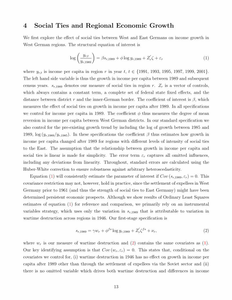
4 Social Ties and Regional Economic Growth

We first explore the effect of social ties between West and East Germans on income growth in

West German regions. The structural equation of interest is

log

(yr,t

yr,1989

)= βsr,1989 + φ log yr,1989 + Z

′

rζ + εr (1)

where yr,t is income per capita in region r in year t, t ∈ {1991, 1993, 1995, 1997, 1999, 2001}.The left hand side variable is thus the growth in income per capita between 1989 and subsequent

census years. sr,1989 denotes our measure of social ties in region r. Zr is a vector of controls,

which always contains a constant term, a complete set of federal state fixed effects, and the

distance between district r and the inner-German border. The coefficient of interest is β, which

measures the effect of social ties on growth in income per capita after 1989. In all specifications

we control for income per capita in 1989. The coefficient φ thus measures the degree of mean

reversion in income per capita between West German districts. In our standard specification we

also control for the pre-existing growth trend by including the log of growth between 1985 and

1989, log (yr,1989/yr,1985). In these specifications the coefficient β thus estimates how growth in

income per capita changed after 1989 for regions with different levels of intensity of social ties

to the East. The assumption that the relationship between growth in income per capita and

social ties is linear is made for simplicity. The error term εr captures all omitted influences,

including any deviations from linearity. Throughout, standard errors are calculated using the

Huber-White correction to ensure robustness against arbitrary heteroscedasticity.

Equation (1) will consistently estimate the parameter of interest if Cov (sr,1989, εr) = 0. This

covariance restriction may not, however, hold in practice, since the settlement of expellees in West

Germany prior to 1961 (and thus the strength of social ties to East Germany) might have been

determined persistent economic prospects. Although we show results of Ordinary Least Squares

estimates of equation (1) for reference and comparison, we primarily rely on an instrumental

variables strategy, which uses only the variation in sr,1989 that is attributable to variation in

wartime destruction across regions in 1946. Our first-stage specification is

sr,1989 = γwr + φfs log yr,1989 + Z′

rζfs + νr, (2)

where wr is our measure of wartime destruction and (2) contains the same covariates as (1).

Our key identifying assumption is that Cov (wr, εr) = 0. This states that, conditional on the

covariates we control for, (i) wartime destruction in 1946 has no effect on growth in income per

capita after 1989 other than through the settlement of expellees via the Soviet sector and (ii)

there is no omitted variable which drives both wartime destruction and differences in income

13

growth post-1989.

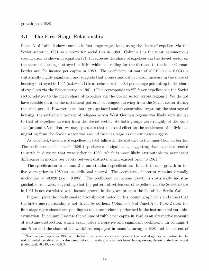
4.1 The First-Stage Relationship

Panel A of Table 2 shows our basic first-stage regressions, using the share of expellees via the

Soviet sector in 1961 as a proxy for social ties in 1989. Column 1 is the most parsimonious

specification as shown in equation (2). It regresses the share of expellees via the Soviet sector on

the share of housing destroyed in 1946, while controlling for the distance to the inner-German

border and for income per capita in 1989. The coefficient estimate of -0.019 (s.e.= 0.004) is

statistically highly significant and suggests that a one standard deviation increase in the share of

housing destroyed in 1945 (s.d.= 0.21) is associated with a 0.4 percentage point drop in the share

of expellees via the Soviet sector in 1961. (This corresponds to 8% fewer expellees via the Soviet

sector relative to the mean share of expellees via the Soviet sector across regions.) We do not

have reliable data on the settlement patterns of refugees arriving from the Soviet sector during

the same period. However, since both groups faced similar constraints regarding the shortage of

housing, the settlement pattern of refugees across West German regions was likely very similar

to that of expellees arriving from the Soviet sector. As both groups were roughly of the same

size (around 3.5 million) we may speculate that the total effect on the settlement of individuals

migrating from the Soviet sector was around twice as large as our estimates suggest.

As expected, the share of expellees in 1961 falls with the distance to the inner-German border.

The coefficient on income in 1989 is positive and significant, suggesting that expellees tended

to settle in districts that were richer in 1989, which is most likely attributable to permanent

differences in income per capita between districts, which existed prior to 1961.18

The specification in column 2 is our standard specification. It adds income growth in the

five years prior to 1989 as an additional control. The coefficient of interest remains virtually

unchanged at -0.020 (s.e.= 0.005). The coefficient on income growth is statistically indistin-

guishable from zero, suggesting that the pattern of settlement of expellees via the Soviet sector

in 1961 is not correlated with income growth in the years prior to the fall of the Berlin Wall.

Figure 1 plots the conditional relationship estimated in this column graphically and shows that

the first-stage relationship is not driven by outliers. Columns 3-5 of Panel A of Table 2 show the

first-stage regressions corresponding to robustness checks performed in the instrumental variables

estimation. In column 3 we use the volume of rubble per capita in 1946 as an alternative measure

of wartime destruction, which again yields a negative and significant coefficient. In columns 4

and 5 we add the share of the workforce employed in manufacturing in 1989 and the extent of

18Income per capita in 1989 is included in all specifications to present the first stage corresponding to theinstrumental variables results discussed below. If we drop all controls from the regression, the estimated coefficientis identical, -0.019, s.e.=0.007.

14

migration after reunification as additional controls. The coefficient of interest remains unchanged

and statistically significant at the 1% level in each case.

Panel B of Table 2 repeats the same specifications as in Panel A, using the share of households

with ties to relatives in East Germany in 1991 from our household level dataset as an alternative

proxy for social ties in 1989. In the interest of preserving space we show only the coefficient of

interest. All estimates are negative and all except the one in column 3 are statistically significant

at the 5% level. The coefficient in column 1 is -0.099 (s.e.= 0.042). It implies that a one standard

deviation rise in the share of housing destroyed in 1945 is associated with a 2.08 percentage point

drop (or alternatively a 9.3% drop relative to the average) in the share of respondents that have

a relative in East Germany in 1991. Similar results (not shown) hold for the share of respondents

that report to be in contact with friends in East Germany. In the remainder of the paper we

use the share of expellees via the Soviet sector in 1961 as our main proxy for social ties since,

coming from a comprehensive survey of the population, we expect it to be measured with less

error than the results from our household level dataset. Needless to say, the correlation between

the two proxies is very high (64%), as shown in Figure 2.

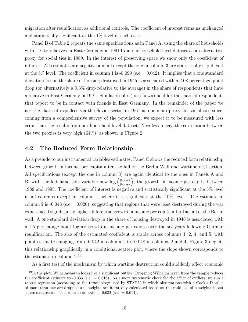
4.2 The Reduced Form Relationship

As a prelude to our instrumental variables estimates, Panel C shows the reduced form relationship

between growth in income per capita after the fall of the Berlin Wall and wartime destruction.

All specifications (except the one in column 3) are again identical to the ones in Panels A and

B, with the left hand side variable now log(

yr,1995

yr,1989

), the growth in income per capita between

1989 and 1995. The coefficient of interest is negative and statistically significant at the 5% level

in all columns except in column 1, where it is significant at the 10% level. The estimate in

column 2 is -0.048 (s.e.= 0.020), suggesting that regions that were least destroyed during the war

experienced significantly higher differential growth in income per capita after the fall of the Berlin

wall. A one standard deviation drop in the share of housing destroyed in 1946 is associated with

a 1.5 percentage point higher growth in income per capita over the six years following German

reunification. The size of the estimated coefficient is stable across columns 1, 2, 4, and 5, with

point estimates ranging from -0.042 in column 1 to -0.048 in columns 2 and 4. Figure 3 depicts

this relationship graphically in a conditional scatter plot, where the slope shown corresponds to

the estimate in column 2.19

As a first test of the mechanism by which wartime destruction could suddenly affect economic

19In the plot, Wilhelmshaven looks like a significant outlier. Dropping Wilhelmshaven from the sample reducesthe coefficient estimate to -0.033 (s.e. = 0.016). As a more systematic check for the effect of outliers, we run arobust regression (according to the terminology used by STATA) in which observations with a Cook’s D valueof more than one are dropped and weights are iteratively calculated based on the residuals of a weighted leastsquares regression. The robust estimate is -0.032 (s.e. = 0.014).

15

growth 50 years later, the specification in column 3 includes both the share of housing destroyed

in 1946 and rubble per capita in 1946. The results are encouraging for our identification strategy:

while the coefficient on the share of housing destroyed remains negative and significant at -0.060

(s.e.= 0.027), the coefficient on rubble per capita is positive and insignificant. This pattern

suggests that it is primarily the lack of housing in 1946 and not wartime destruction per se that

affects economic growth post 1989.

4.3 Instrumental Variables Results

In our instrumental variables estimation we explicitly test the main hypothesis of this paper:

that the intensity of social ties between East and West Germans in 1989 is causally related to

a rise in income per capita after the fall of the Berlin Wall. In Table 3, we estimate (1) using

only the variation in the social ties in 1989 that is due to variation in wartime destruction, by

instrumenting for the share of expellees via the Soviet sector in 1961. In column 1 we instrument

with the share of housing destroyed in 1946. The coefficient estimate for the share of expellees is

2.169 (s.e.= 0.947), suggesting that a one standard deviation increase in the share of expellees in

1961 (s.d.= 0.019) is associated with a 4.3% rise in income per capita over the six years following

1989 (or roughly a 0.7 percentage point higher rate of growth per annum).20 The coefficient

on income in the base year, 1989, is negative and significant, which suggests mean reversion in

income per capita across West German districts. Somewhat surprisingly, the coefficient on the

distance to the inner-German border is positive, which suggests that the districts closest to the

inner-German border did not immediately profit from the opening of the border (which is in line

with a similar observation in Redding and Sturm (2008), that the population of West German

cities close to the inner-German border grew relatively little between 1989 and 2002).

Column 3 gives our standard specification in which we control both for the level of income

in 1989 and for income growth in the five years preceding 1989. The coefficient of interest rises

slightly to 2.442 (s.e.= 0.880) and is now significant at the 1% level.21 The fact that we control for

both for the pre-existing income level and for pre-1989 income growth means that this estimate

is specific to the period after the fall of the Berlin wall: It can neither be explained by mean

reversion in income growth nor by a pre-existing trend. After the fall of the Berlin wall, there

is a sudden improvement in the growth trajectory of the districts that were least destroyed 50

years earlier, over and above any pre-existing growth trend.22

20The F-statistic against the null that the excluded instrument is irrelevant in the first-stage regression is 22.56(this is the squared t-statistic from Table 2).

21We do not cluster the standard errors at the federal state level as there are only 10 federal states. However,the results presented throughout this section are generally robust to doing so. For our standard specification theclustered standard error is 1.288, which implies that the coefficient of interest remains statistically significant atthe 10% level.

22 Since our model contains a lagged dependent variable there may be a mechanical bias in the coefficient of

16

The results of column 3 are almost unchanged when we simultaneously instrument the share of

expellees with both the share of housing destroyed and with rubble per capita (shown in column

4). Column 2 shows the OLS estimate of our standard specification for comparison. It is only

about one half of a standard error lower at 1.963 (s.e.= 0.574), suggesting that the endogenous

assignment of expellees to West German districts induces only a relatively mild downward bias

in the OLS estimate. A Hausman test fails to reject the null hypothesis that Cov (sr,1989, εr) = 0.

4.4 Validity of the Exclusion Restriction

While the endogenous assignment of expellees to West-German districts does not seem to have a

large impact on our results, our identifying assumption, that the degree of wartime destruction

in 1945 affected growth in income per capita after 1989 only through its effect on the intensity

of social ties in 1989, cannot be tested directly. Nevertheless, we can perform a number of

falsification exercises to assess its plausibility. There are two types of potential challenges and

corresponding tests.

Pre-Trend Tests

The ‘simple’ challenge to our identifying assumption is that wartime destruction (or an omitted

variable driving it) may have had a lasting effect on income growth in West German regions

which persisted for more than half a century (until 1995). We believe that we can convincingly

discard this ‘simple’ challenge.

First, our standard specification controls for the growth rate of income pre-1989 and thus

identifies changes in the region-specific growth trajectory that occur after 1989.

Second, the conventional wisdom in the literature is that wartime destruction had no lasting

impact on West German growth past 1960 (Brakman, Garretsen, and Schramm (2004)). Figure 4

replicates part of this result. It shows coefficient estimates of regressions relating the population

growth in West German cities to wartime destruction in 1946 for various years since 1929.

Not surprisingly, wartime destruction had a strong and significant negative effect on population

growth during the war (between 1939 and 1945). During the period of reconstruction between

1946 and 1960 the cities most heavily destroyed grew fastest. However, from 1960 onwards

there is no statistically significant effect of wartime destruction on population growth and the

coefficient estimates are virtually zero. To the extent that population growth is correlated with

income growth, this result suggests that the effects of war destruction on income growth were

short lasting.

interest. In principle we can instrument for the lagged dependent variable as suggested by Anderson and Hsiao(1982). However, we do not have sufficient pre-1989 data to do this for the specification in column 3. However,we can use income in 1985 as instrument for income in 1989 in the specification of column 1. The coefficientestimate increases slightly to 2.289 (s.e.=0.984) and remains significant at the 5% level.

17

Third, for the short period pre-1989 for which we do have income data we can easily test

for a trend in growth before 1989 that may be correlated with wartime destruction. In Table

4 we use the full panel structure of our data set by regressing log income per capita for each

district and year post-1985 on the interaction of year fixed effects with the share of expellees in

1961, income per capita in the base year (1985), a full set of state-year fixed effects, and the

distance to the inner-German border. The share of housing destroyed in 1946, interacted with

year fixed effects, are the excluded instruments. Here we use a two-step GMM estimator which

accounts for first-order autocorrelation in the error structure. As in our simpler specifications

from Table 3, the coefficients on the interacted variables estimate the effect of social ties on

income growth between 1985 and each of the following census years. In column 1 we see that

there is a negative and insignificant effect of the share of expellees on growth between 1985 and

1987 (-0.329, s.e.= 1.023). The effect changes sign in 1989 (0.506, s.e.=1.022), grows further in

1991 (1.532, s.e.=1.022) and finally becomes statistically significant in 1993 (2.059, s.e.=1.022)

and 1995 (2.813, s.e.=1.023). Columns 2 and 3 show alternative specifications which use 1987

and 1989 as base years, with very similar results. There is thus no evidence of a pre-trend in

growth that would be correlated with wartime destruction, and the timing of the effect is highly

supportive of the view that variation in the degree of wartime destruction only became relevant

after the fall of the Berlin Wall.

Controlling for Alternative Channels

The more ‘sophisticated’ concern about our results is that the pattern of wartime destruction

(or some omitted variable driving it) affected income growth through some other channel which

only switched on post-1989.

One such possibility is that the allies may have bombed areas that were highly industrialized

and the manufacturing sector may have experienced a relative decline in those areas after 1989.

To address this potential concern, the specification in Table 3 column 5 controls for the share of

the population that works in manufacturing in 1989. Indeed, the estimated coefficient on this

variable is negative and significant, picking up a relative decline of highly industrialized districts,

but the coefficient of interest is virtually unaffected by this additional covariate. The variation

in income growth post-1989 due to the relative decline of manufacturing is thus unrelated to

the variation in income growth post-1989 due to the settlement of expellees in West Germany.

In addition, Figure 4 shows that wartime destruction was uncorrelated with pre-war population

growth. To the extent that we can interpret take pre-war population growth as an indicator

for economic growth more generally, this would suggest that allied bombings during World War

II were not specifically targeted at destroying cities which were on a higher or lower growth

trajectory.

Another potential concern is that after 1989 highly skilled workers from East Germany may

18

have migrated to the same districts in which their relatives settled before 1961, and that this

migration may have increased the average wage paid in these districts. In column 6 we control

for the flow of migration from East to West, and again there is little effect on the coefficient of

interest.23

Placebo Test

While neither of these two likely channels seem to be driving our results, there might be other

omitted variables which are correlated with the pattern of wartime destruction and post-1989

deviations from the existing growth trajectory. Furthermore, we may be misinterpreting our

results in that expellees may affect income growth after 1989 through some channel other than

social ties, which switches on post-1989. In particular, expellees might have been somehow

different from other Germans, and these different traits (a higher propensity to become an

entrepreneur, different preferences, etc.), put them in an advantageous position to earn higher

incomes post 1989 for reasons unrelated to social ties to the East. We are able to provide evidence

on this, and in fact the entire class of ‘sophisticated’ challenges, by comparing the expellees via

the Soviet sector with expellees who arrived directly from the annexed parts of pre-war Germany.

The direct expellees migrated from the same areas in Eastern Europe, they look very similar to

expellees via the Soviet sector on observable characteristics, and their settlement pattern was

affected by wartime destruction in a similar way. The only relevant difference between the

two groups is that expellees who arrived directly from the annexed areas did not spend any

significant time living (and forming social ties) in East Germany. If we misinterpret our results

and the effects we document are driven by some omitted variable which determined both wartime

destruction and post 1989 income growth, or if there was something special about expellees per

se that gave them access to business opportunities post-1989, we would expect to find the same

effects for both the expellees via the Soviet sector and the direct expellees.24

Table 5 shows summary statistics on both groups of expellees from the 1971 census, the last

census in which the two groups are separately identified. The table gives the average income,

the average number of years of schooling, and the occupational structure of the ‘native’ West

German population (column 1) and of both groups of expellees (columns 2 and 3). While both

groups of expellees have slightly lower income in 1971 than the native West German population,

the average income of direct expellees and expellees who arrived via the Soviet sector is similar

(DM 777.8 and DM 764.4 per month, respectively). Similarly, both groups of expellees have

23When we use the flow of migration from East Germany as the dependent variable, the coefficient on expelleesis not significant, which is comforting for our interpretation of the results. A related result in the literature isthat high-skilled workers from the East were actually less likely to migrate to the West than low-skilled workersup until 1996 (Fuchs-Schundeln and Schundeln (2009)).

24Recall from our discussion in section 2 that expellees were allocated to the four sectors according to quotasand that, as far as we can tell from the statistics published in East Germany, the vast majority of expellees whowere allocated to the Soviet sector migrated to the West before 1961.

19

relatively fewer entrepreneurs among them and a lower representation in agriculture than the

native West German population, but the occupational structure of direct expellees and expellees

via the Soviet sector is extremely similar.

To compare the effect of direct expellees and expellees via the Soviet sector we require a

second instrument, which gives us differential leverage in identifying the exogenous components

in the settlement patterns of both groups. In columns 1 and 2 of Table 6 we re-run our standard

first-stage regression from Table 2 column 2, but include both the share of housing destroyed and

the volume of rubble per capita in 1946. (We again do not report covariates in the interest of

space.) Column 1 gives the results for expellees arriving via the Soviet sector and column 2 gives

the results for expellees arriving directly in West Germany. In the case of the former, the share

of housing destroyed is significant with a negative sign and rubble is insignificant. In the case of

the latter, the size of the effect of the share of housing destroyed is roughly preserved, though it

is less precisely estimated. However, importantly for us, the coefficient on the amount of rubble

is negative and significant. Our two measures of wartime destruction thus give us differential

leverage in identifying the exogenous components in the settlement patterns of both groups. We

believe that this feature of the data is related to the timing of the arrival of the two groups of

expellees. The direct expellees arrived immediately after the war and the expellees via the Soviet

sector arrived between 1945 and 1961. We suspect that rubble per capita measures a dimension

of wartime damage which was important in the immediate aftermath of the war but then cleared

away relatively quickly (many German cities famously have ‘rubble mountains’ which were piled

up in the first two to three years after the war), while the share of housing destroyed had a longer

lasting effect on the settlement of expellees.

Using both instruments, we are thus able to separately estimate the effect of expellees who

arrived via the Soviet sector and the effect of direct expellees on differential income growth after

1989. Column 3 presents the result. While the coefficient on the share of expellees who arrived

via the Soviet sector is positive, similar in magnitude to the estimates obtained earlier (3.422,

s.e.= 1.809), and statistically significant, the coefficient on the share of direct expellees is close to

zero and statistically insignificant. Since both groups are extremely similar, except for the fact

that expellees who spent a number of years in the Soviet sector had an opportunity to form social

ties with East Germans, we view this result as strong support in favor of our interpretation.

4.5 Remaining Caveats

A remaining caveat to our results is that they are also consistent with two proximate interpre-

tations which we do not emphasize due to our reading of German history. First, the results

might document the value of ‘local knowledge’ about East Germany. In principle, the effects we

document could be driven by individuals who lived in East Germany during their youth, do not

20

have personal contact with anyone there, but remember enough details about the local economy

to earn rents after reunification. We do not emphasize this interpretation as the conventional

view is that economic conditions in East Germany have changed dramatically between 1961 and

1989, so that local knowledge acquired before the division of Germany would be useless after 40

years of socialist rule. Moreover, our individual-level results show that even households headed

by individuals who were too young to remember living in East Germany experience a rise in their

personal income after 1989 if they have a relative in the East, providing some partial evidence

against this alternative interpretation.

Second, some of the rise in household and regional income may be driven by restitutions and

payments of compensation to those whose property had been expropriated in East Germany.

Under the reunification treaty, former owners of firms and real estate could apply for restitution

providing that they had not received compensation from the East German government and the

assets they were claiming still existed at the time of filing a claim. This meant that practically

all individual claims made related to buildings and land. While there were a large number of

claims filed (around 2 million), we do not believe that restitution or compensation payments

could be responsible for the patterns we document in the data.

The administrative backlog created by the task of tracing ownership rights over a period of

50 years was so enormous that it was not sufficiently cleared in time to confound the effects we

document (in fact, the authorities and courts are still processing claims to the present day). The

first compensation payments were not set to begin until 1996, whereas the effects we document

begin immediately after 1989 (Southern (1993)). The only real concern is thus the existence of

cases in which the filing of a claim resulted in the restitution of a property prior to 1995, and

the restitution of this property resulted in a rise in income. The early restitutions were mainly

of firms, as the establishment of safe property rights for productive assets was a political priority

(although even these were the subject of protracted legal battles, so that in 1992, 90% of claims

concerning firms were still on hold due to litigation; see Sinn and Sinn (1992)).

We address this concern by calculating an upper bound for the value of all restitutions that

could possibly have been made in the period in question and comparing it to the magnitude

of the effects that we attribute to social ties. According to the government agency handling

restitutions, half of all approved claims had been settled by restitution, and the total sum of

compensation payments made between 1990 and 2009 was EUR 1.4 bn.25 These compensation

payments were made at about 50% of market value, and so a reasonable estimate of the value

of all restitutions is therefore EUR 1.4bn0.5

=EUR 2.8bn. Assuming that all restitutions had been

completed before 1995 (which they were not) and assuming that the new owners immediately sold

25Personal correspondance with Dr. Handler, press liaison of the Bundesamt fuer zentrale Dienste und offeneVermogensfragen.

21

the returned assets on (which they were often legally prevented from doing), aggregate income

in West Germany could thus have risen at most by EUR 2.8bn. This number is an order of

magnitude smaller than the total effect implied by our regional level results (around EUR 74.0

bn in 1989 equivalents of Euros).

5 Understanding the Effect on Regional Economic Growth

5.1 Entrepreneurial Activity

In an effort to shed light on the channel linking social ties to regional economic growth, we

disaggregate regional income per capita into the average income of households whose primary

income derives from entrepreneurial activity (entrepreneurs) and the average income of all other

individuals (non-entrepreneurs) for each year.26 In columns 1 and 2 of Table 7 we re-run our

standard specification from column 3 in Table 3 with the growth rate in the average income of

each of these groups as the dependent variable. Both specifications include the same covariates

as our standard specification, but add the (log of the) average income of entrepreneurs and non-

entrepreneurs in 1989, respectively, as an additional control. The coefficient estimate is 4.008

(s.e.= 2.096) for entrepreneurs (column 1) and 1.755 (s.e.= 0.735) for non-entrepreneurs (column

2); suggesting that a one standard deviation rise in the share of expellees via the Soviet sector is

associated with a 7.6% rise in the average income of entrepreneurs, but only a 3.3% rise in the

average income of non-entrepreneurs. Entrepreneurs who lived in a region with strong social ties

to the East thus experienced a much steeper rise in their average income than non-entrepreneurs

living in the same region.27

This strong effect on the income of entrepreneurs is mirrored by an increase in the number

of entrepreneurs. In column 3 we re-run our standard specification but use the share of the

population that are entrepreneurs in 1995 as the dependent variable, where we again add the

share of the population that are entrepreneurs in 1989 as an additional control. The coefficient

of interest is 0.322 (s.e.=0.163), suggesting that a one standard-deviation rise in the share of

expellees in 1961 (0.019) induces a 0.61 percentage point rise in the share of the population

which are entrepreneurs. This is a sizable effect, corresponding to a 14.2% rise relative to the

26In the German Mikrozensus these are households whose household heads declare that their primary occupationis ‘entrepreneur’ (Selbststaendiger mit oder ohne Beschaeftigte).

27The residuals of the specifications in column 1 and 2 of Table 7 are likely to be correlated. If we estimate thetwo equations as well as the first stage jointly with a 3SLS estimator, the results are considerably reinforced. Inparticular, the coefficient of interest in column 1 rises to 4.920 (s.e.= 1.657) and is significant at the 1% level. Incolumn 2 the coefficient of interest is estimated to be 1.451 (s.e.= 0.665) and significant at the 5% level. In thesespecifications we control for the (log of the) average income of entrepreneurs and non-entrepreneurs in 1989 inboth structural equations of interest and the first stage. The null of equality of these coefficients is rejected atthe 5% level.

22

mean share of entrepreneurs in 1989 (0.043).

5.2 Firm Investment

The strong rise in entrepreneurial income in regions with strong social ties to the East suggests

that firms which were based in these regions must have generated higher profits in the years

following the fall of the Berlin Wall. One possible reason for such a rise in profitability is that

being based in a region with strong social ties to the East may have generated a comparative

advantage in investing in the East. Firms who had access to a workforce or to an owner with

strong social ties to the East may have been in a better position to estimate the value of East

German firms that came up for sale or may have been better able to gauge demand for Western

products and services. We explore this possibility by examining the subsidiaries and branches

that West German firms operated in eastern Germany in 2007, which is the earliest year for

which we were able to obtain detailed data at the firm level.

From the universe of West German firms in 2007 we select the 19,402 firms whose headquarters

are located in West Germany and who operate at least one subsidiary or branch in West Germany.

For these firms we calculate a dummy variable which is one if the firm operates a subsidiary or

branch in East Germany and zero otherwise. Since West German firms could not own assets in

East Germany prior to the fall of the Berlin Wall, any subsidiaries or branches that they operate

in 2007 must have been acquired after 1989. Our dummy variable is thus informative both about

the investment behavior of West German firms in East Germany since 1989 and about a possible

long-lasting effect of social ties in 1989 on the economic structure of West Germany.

The structural equation of interest is

bkdr,2007 = βfsdr,1989 + φf log yd,1989 + Z′

kdrζf + εf

kdr (3)

where bkdr,2007 stands for the dummy indicating whether firm k in West German district d and

region r operates a subsidiary or a branch in East Germany in 2007. sdr,1989 is again our measure

of social ties between the residents of district d in region r and East Germany in 1989; yr,1989

stands for income per capita in region r in 1989; and Zkdr is a vector of firm and district level

controls which contains a complete set of federal state fixed effects, a fixed effect for the sector

in which the firm has its primary operations, the log of the number of subsidiaries and branches

that firm k operates in West Germany, and the distance between district d and the inner-German

border. Note that income per capita in 1989 is available only at the regional level and not at the

district level.

The coefficient of interest is βf which measures the effect of the intensity of social ties to

the East in a given West German district in 1989 on the probability that a firm headquartered

23

within that district operates a subsidiary or branch in East Germany in 2007. As in section 4,

we account for the possibility that our measure of social ties (the settlement of expellees via the

Soviet sector in West Germany) is jointly determined with income growth, and instrument for

sdr,1989 with the share of housing destroyed in 1946. The first stage of our instrumental variables

strategy is thus the analog to (2). We cluster all standard errors at the district level to account

for likely spatial correlation.

Panel A of Table 8 shows reduced form estimates, relating the share of housing destroyed in

1946 directly to the probability that a given firm operates a subsidiary or branch in East Germany

in 2007. In column 1, we regress our dummy variable on the share of housing destroyed in the

district and the log of the number of subsidiaries and branches that the firm operates in West

Germany in 2007, which we use as a simple control for the size of the firm.28 The coefficient of

interest is -0.030 (s.e.=0.011) and statistically significant at the 1% level. The estimate implies

that a one standard deviation rise in the extent of wartime destruction within a given West

German district is associated with a 0.7% drop in the probability that a firm based in that

district operates a subsidiary or branch in East Germany in 2007.29 Unsurprisingly, larger firms

are more likely to operate subsidiaries and branches in East Germany, which is reflected in

a positive coefficient on our size control. Columns 3-6 add all of the now familiar district and

region level covariates from section 4, and column 3 gives the analog of our standard specification.

Throughout, the coefficient of interest remains in a tight range between -0.029 and -0.031 and

statistically significant at 1%.

Panel B shows our instrumental variables estimates of equation (3), which use the variation in

wartime destruction to quantify the causal effect of social ties in 1989 on the investment behavior

of West German firms. All specifications contain the same covariates as those in Panel A. The

estimates in all columns are positive and all are statistically significant at the 5% level. The

estimate from our standard specification in column 3 is 1.556 (s.e.= 0.693), which implies that a

one standard deviation rise in the share of expellees in a West German district is associated with

a 3.4% increase in the probability that a firm based in that district will operate a subsidiary or a

branch in East Germany in 2007.30 This link between the pattern of social ties in 1989 and the

investment behavior of West German firms offers a potential explanation for why residents of

districts with strong social ties to the East, and entrepreneurs in particular, may have experienced

a rise in their incomes. The increased firm level activity also suggests potential spill-over effects

of social ties, i.e. residents of districts with strong social ties to the East might experience a rise

in income even if they themselves did not have social ties to the East. We return to this issue in

28The raw correlation between our dummy variable and the share of housing destroyed is -0.019 (s.e.=0.012)and statistically significant at the 10% level.

29The standard deviation of the share of housing destroyed at the district level is 0.24.30The district level standard deviation of the share of expellees via the Soviet sector is 0.022.

24

the following section where we calculate the size of such potential spill-over effects.

The remaining panels of Table 8 show the results of a number of falsification exercises. These

are based on the idead that if the pattern in holdings of subsidiaries and branches prevailing in

2007 is truly attributable to the intensity of social ties to East Germany in 1989, and not to

some other factor, our measure of social ties to East Germany should not predict investment in

other areas of the world.31 Panels C-F repeat the same specifications as in Panel B, but with

a dummy variable indicating whether a firm has subsidiaries or branches in Poland, in the ‘old’

EU countries (the 14 member countries other than Germany prior to the enlargement in 2004),

in the ‘new’ EU countries (the 9 countries, other than Poland, which joined the EU in 2004), or

in non-EU countries as the dependent variable. As expected, all estimated coefficients in Panels

D, E and F are statistically insignificant. Firms which are based in districts with a high share

of expellees are thus not more likely to operate subsidiaries or branches in areas other than East

Germany. Interestingly, however, the only exception from this rule is that the estimates for

Poland are positive and statistically significant at the 5% level in all columns. The estimated

effect for Poland is about 1/5th the size of the effect estimated for East Germany. Since the

largest group of expellees who settled in West Germany after 1945 actually came from areas that

are today part of Poland, these results suggest a possible additional effect of social ties to Poland

on the investment behavior of West German firms.32 33

6 Social Ties and Household Income

Lastly, we explore how individual households may have profited from having ties to East Germany

and how these ties may have affected regional economic growth. We use the German Socio-

Economic Panel (SOEP) dataset and select households which were in the panel in 1985, located

in West Germany in 1989 and remained in the panel at least until 1995. The 1991 wave of the

panel contains several questions about contacts with friends and family in East Germany. Since

the survey was conducted in the second year after the fall of the Berlin Wall and individuals had

some time to renew ties with individuals in the other part of Germany, we choose not to rely

on information about the intensity of contact to friends and relatives, although it is available.34

31If firms from districts with a high fraction of expellees were merely good at capitalizing on new businessopportunities, regardless of social ties, we might, for example, expect to see an effect on their holdings in otherEastern European countries following consecutive rounds of EU enlargement.

32However, the size of the coefficient for Poland is similar to that of some of the other, insignificant coefficients.33Table A.2 in the appendix reports the outcomes of additional robustness checks, in which we repeat the same

specifications as in panels A and B of Table 12, but now use the share of each firm’s subsidiaries and branchesoperated in East Germany as the dependent variable. The results are again similar, indicating that firms whichare headquartered in West German districts that have strong social ties to East Germany in 1989 also operate alarger share of their subsidiaries and branches in East Germany today.

34Our results are very similar if we use this information on friendships or condition on respondents indicating‘close’ ties to their relatives or friends.

25

Instead, we base our work on the response to the simple factual question: ”Do you have relatives

in East Germany?”, and generate a dummy variable that is one if at least one member of the

household responded with ‘yes’ and zero otherwise. A possible source of measurement error

is that some West Germans may have migrated to East Germany directly after the fall of the

Berlin Wall and before the conclusion of the 1991 wave of the survey. However, our data indicate

that the flow of migrants from West to East in 1990 was not large enough to plausibly induce

a quantitatively large bias. It is thus safe to assume that households which were based in West

Germany in 1989 and report a relative in East Germany in 1991, also had a relative in East

Germany in 1989.

Table 10 gives summary statistics for the entire panel of 1911 households, and for the sub-

sets of households which report and do not report any ties to relatives in East Germany. The

households with ties to East Germany had slightly lower income in 1989 (DM 3219 versus DM

3491 per month in 1989) and the household heads of households with ties to East Germany tend

to have had slightly less education (on average 12.12 years versus 12.42 years). However, the

two subsets of households look very similar on other observable dimensions: they had about the

same amount of capital income on average, and the proportion of households whose head was

reported as entrepreneur was similar across the two subsets, as was the proportion reported as

unemployed.

Our basic household level regression estimates the growth in household income that results

from having social ties to East Germany in 1989:

log

(yi,t

yi,1989

)= βhhTi + φhh log yi,1989 + Z

′

iζhh + εi, (4)

where yi,t is the income of household i in year t, Ti is a dummy variable indicating ties to East

Germany and Zi is a vector of controls which contains a full set of district fixed effects, household

income growth between 1985 and 1989, and the gender, age and age squared of the household

head. The coefficient of interest is βhh which estimates the effect of ties to relatives in East

Germany on the growth in household income after 1989.

Before estimating (4), Table 11 establishes the consistency of our household level and region

level datasets. Column 1 reproduces the standard specification from Table 3 column 3, in which

we related region-level income growth to the share of expellees in the district in 1961, regional

average income in 1989, regional average income growth prior to 1989, and the distance of the

region to the inner-German border. In column 2, we regress household level income growth on the

same region level covariates, as well as on household level income in the base year and household

level income growth between 1985 and 1989. The coefficient estimate on share expellees is

insignificant, but remarkably similar to the one we obtained in the district level dataset, 2.777

26

(s.e.= 3.609). The fact that the estimate is statistically insignificant is not surprising as we are

now using a sample of 1911 households, rather than district averages of 1% of the population.

However, it is comforting that both datasets seem to have similar quantitative implications in

this regard.

In column 3 we drop the region level share of expellees variable and replace it with a household

level dummy variable indicating ties to East Germany. The estimate is positive and highly

statistically significant, 0.069 (s.e.= 0.025). However, our dummy variable indicating ties to

East Germany is mechanically correlated with the average level of social ties in a given district.

The coefficient estimate in column 3 may therefore confound the direct (household) effect of

having ties to the East with possible spill-over effects from other households in the same region

having social ties.

We therefore introduce a full set of region fixed effects in column 5, which absorb the region

wide effect of a higher incidence of social ties. Additionally we control for gender, age and

age squared of the household head (which are standard controls in the labor literature) and

estimate the full model in (4). The coefficient of interest drops to 0.049 (s.e.= 0.023) and

remains statistically significant at the 5% level. The point estimate indicates that households

with ties to East Germany in 1989 experienced on average a 5 percentage points higher income

growth in the 6 years following the fall of the Berlin Wall relative to comparable households

without such ties.

For specification (4) to consistently estimate the coefficient of interest we require cov (Ti, εi) =

0. As social ties existing prior to 1989 must have been maintained for reasons unrelated to any

expected economic benefit, this condition does not fail due to reverse causality. However, it

may still fail if individuals with social ties have some omitted characteristics which affect income

differently after 1989 as compared to before 1989 and are correlated with social ties. In particular,

individuals with social ties might somehow be more entrepreneurial or better educated, and

therefore better able to seize the economic opportunities that present themselves after the fall

of the Berlin Wall.35 The summary statistics in Table 10 suggest the opposite: the heads of

households with social ties to the East were actually slightly less educated and were somewhat

less likely to be an entrepreneur in 1989. We control for these observable characteristics in our

robustness checks discussed below.

In Table 12 we add a number of additional covariates (again this table only reports the

35A second reason why the estimation might be inconsistent is that we include a lagged dependent variable,which might be correlated with an auto-correlated error. We cannot perform Arellano-Bond style estimationas we do not have enough pre-1989 data. However, when running a specification in which we control for thehousehold income in 1989, but not for the pre-existing growth trend, we can instrument for household income in1989 with household income 1985. When running a specification equivalent to column 5 in Table 11, but withoutcontrolling for growth between 1985 and 1989, the coefficient of interest is estimated to be 0.049 (s.e.=0.023).When instrumenting for household income in 1989 with household income in 1985 the coefficient of interest isestimated to be 0.038 (s.e.=0.022) and significant at the 10% level.

27

coefficient of interest and the coefficients on the variables that are added relative to the standard

specification). Column 1 reproduces the standard specification for comparison. Column 2 adds

years of education and years of education squared of the household head in 1989, both of which

remain statistically insignificant. Column 3 adds the log of capital income in 1989 as a proxy

for the household’s ability to finance investments. The variable is positive and significant, but

induces little change in the coefficient of interest which remains at 0.047 (s.e.= 0.023). Column

4 introduces a dummy variable for whether the household head is an entrepreneur. Surprisingly,

this variable remains insignificant, and again induces almost no change in the coefficient of

interest. Finally, in column 5 we add a dummy for household heads who are not in employment

in 1989 and column 6 adds all of these additional covariates simultaneously. Throughout, the

changes in the coefficient of interest are minor and it remains statistically significant at the 10%

level.

In Figure 5 we explore the timing of the effect by again using the full panel structure of the

data in a specification analogous to Table 4 column 1.36 We regress the income of each household

in a given year on its income in 1985, a full set of year and district fixed effects, the interaction

of year effects with the dummy variable indicating ties to East Germany in 1991, and controls

from our standard specification (gender, age and age squared). The figure plots the interaction

of year fixed effects with the dummy for ties to relatives in 1991, and identifies a 5% confidence

interval.37 These interactions measure the differential income growth of households with social

ties to the East between 1985 and the indicated year. The pattern is striking: the estimates are

statistically indistinguishable from zero until 1989, when the estimates jump up and are mostly

statistically significant at the 5% level until 1995. All coefficients after 1989 are statistically

significant at the 10% level until the end of the sample in 2001.

Lastly, we can check that our results are robust to potentially confounding restitutions of

assets from the East. The claimants who were likely to have received their assets by 1995, the

year on which we focus in our analysis, are those whose claim related to a firm. If we re-run our

standard specification in Column 5 of Table 11, dropping all households that state not to own

productive assets in 1989, but state to own productive assets in 1995, the coefficient drops only

very slightly to 0.047 (s.e.= 0.023).38 The household level results are thus robust to excluding

the subgroup of observations that could plausibly have benefited from restitutions prior to 1995.

This adds to the evidence presented in section 4.4 that restitutions are unlikely to drive our

results.

36Although we use a standard fixed effects estimator as all of our covariates are exogenous37The sample size is decreases monotonically from 1911 in 1995 to 1419 in 2001.38A total of 57 households in our sample acquired productive assets between 1989 and 1995, 17 of which had

relatives in East Germany.

28

6.1 Cohort Heterogeneity

Our sample contains only 596 households with ties to the East. Nevertheless, we are able to give

some further evidence on why the income of individual households increased after 1989. In Table

13, we estimate our standard specification, but interact the dummy for ties to East Germany with

a fixed effect for the age quartile of the household head (and naturally also add fixed effects for

each age quartile on the right hand side). The coefficient estimate for the youngest age quartile

(those aged below 40 in 1989) is positive and significant at the 10% level, 0.092 (s.e.= 0.051).

This is particularly interesting as it indicates that the effect we estimate is about knowing people

and not about knowing places: the household heads in this group were younger than 11 years

old at the time when the Berlin Wall was built and thus could not have had much personal

experience of living in East Germany. However, they could easily have kept in contact with their

relatives in East Germany.

6.2 East German Households

We have presented evidence on the returns to social ties accruing in West Germany. Naturally,

we are interested in the corresponding effects in East Germany. Due to a lack of data on the

settlement of expellees and on outcome variables prior to 1990, we cannot replicate our region

level results for East Germany. However, we can replicate part of our standard specification in

column 5 of Table 11 for households in East Germany. In particular, Table 14 shows results for a

regression relating log income of East German households in the years after German reunification

to a dummy variable indicating relatives in West Germany in 1991 and all household level

covariates of column 5 in Table 11 other than income in 1989 and pre-1989 income growth. As

we have no data on income before 1990 for East German households, this specification can only

speak to differences in levels of income, rather than to differences in income growth. Nevertheless,

we find that the estimate on the coefficient of interest is positive in all years between 1990 and

1995 and marginally significant in two of the six years (1992 and 1994). For example, the estimate

for 1995 is 0.057 (s.e.=0.040) suggesting that East German households with ties to the West tend

to have higher income than those without ties to the West.

6.3 Spill-over Effects

The household level effect we estimated in this section is economically large. However, it is not

large enough to account for the size of the entire region level effect of social ties estimated in

section 4. Since the district level standard deviation of the share of households with social ties

to the East is 0.10 (see Table 1), a one standard deviation rise is thus associated with at most a

0.7 percentage point rise in income per capita at the region level (Table 11, column 3). To the

29

extent that the variation in the level of social ties in 1991 is driven by variation in the share of

expellees (recall that the correlation between our two measures of social ties is very high), a one

standard deviation rise in the share of households with relatives in East Germany corresponds

to the same variation as a one standard deviation rise in the share of expellees in a district.

However, a one standard deviation increase in the share of expellees in 1961 was associated with

a 4.3 percentage point rise in district level income. The two estimates suggest a spill-over effect

by which households without ties profit from living in a district with strong ties to the East.

This spill-over is consistent with the view that firms which were based in regions with strong

social ties had an advantage in investing in East Germany, which resulted in increased wage

levels in those West German districts. The presence of spillovers might also imply that social

ties have an economic value even at the second or third degree of separation, where a household

(and entrepreneurs in particular) might profit from having a social tie to another household who

has a social tie to East Germany.39

7 Understanding the Microeconomic Effects

While we were able to provide a range of evidence suggesting that social ties facilitated regional

economic growth by generating a rise in entrepreneurial activity, a deeper question is why social

ties matter at the individual level. Two potential channels linking social ties to economic perfor-

mance at the microeconomic level are that (i) social ties may reduce informational asymmetries

(Granovetter (1973), Varian (1990), Stiglitz (1990)) and (ii) social ties may sustain a large range

of credit contracts that would otherwise not be feasible (Besley and Coate (1995)). In our con-

text, possible examples of these stories might be (i) a West German who hears from his East

German cousin about the lack of second hand cars in East Germany and reacts by starting a

local car dealership in the East or (ii) a wealthy West German who lends his own money or acts

as a guarantor for a East German relative who otherwise would not have access to funds.

One way to gauge the relevance of the first mechanism is to test whether social ties are

particularly beneficial for firms in sectors in which informational frictions are important. In Table

9 we return to the standard specification of our firm level analysis (Table 8, Panel B, column

3) and replace the share of expellees variable with its interaction with each of the four sectoral

fixed effects included in the specification (instrumenting these variables with the interactions of

the sectoral fixed effects and the share of housing destroyed in 1946). The estimated effects in

the Primary, Government, and Manufacturing sectors are statistically insignificant, while the

effect estimated for the Trade and Services sector is positive and statistically significant at the

5% level (0.962, s.e.= 0.449). We may interpret this as evidence that social ties were particularly

39A novel by Schulze (2005) presents an example of such interaction at the second degree of separation.

30

important for firm investment in the Trade and Services sector, which is arguably the sector of

the economy which is most susceptible to informational asymmetries and reliant on knowledge

of local demand.40

We may evaluate the relevance of the second channel by testing whether the West German

households who had the highest ability to fund or act as guarantors for projects in the East were

also the ones to benefit most from their social ties to the East. Column 1 of Table 15 replicates

the standard specification of our household level results from Table 11, column 5 (again reporting

only the coefficient of interest). In columns 2-4 we add a dummy which is one if the household’s

capital income in 1989 is above the pth percentile (75th, 95th and 99th, respectively) as well as the

interaction of this variable with our dummy for social ties. If the principal function of social ties

was to enhance households’ ability to enter into credit contracts we would expect the coefficient

on the interaction term to be positive. In column 2 the point estimate on our social ties dummy

drops marginally to 0.46 (s.e.=0.026) and remains significant at the 10% level. The dummy

indicating top-quartile capital income in 1989 is estimated to have a positive, but insignificant

significant effect on post reunification growth in household income (0.046, s.e.= 0.028). However,

the interaction of social ties and the above-median wealth dummy is insignificant. Columns 3

and 4 show similar results, using the 95th and 99th percentile. This evidence suggests that West

German households benefited from their ties to East Germans regardless of their wealth in 1989

and, consequently, that social ties may have acted mainly as conduits for information rather than

a form of ‘social’ collateral which would serve to sustain credit contracts.

8 Discussion

In this paper we used evidence from German reunification to establish a causal link between

social ties and regional economic development. West German regions which, for idiosyncratic

reasons, have strong social ties to East Germany at the time of the fall of the Berlin Wall exhibit

substantially higher growth in income per capita in the early 1990s. This effect on regional

economic growth appears to be driven both by a rise in the profits accruing to entrepreneurs and

by an increase in the share of the population engaging in entrepreneurial activity. Consistent

with these findings, we show that firms headquartered in a West German district which has

strong ties to East Germany in 1989 are more likely to operate a subsidiary or a branch in East

Germany today, suggesting that the pattern of social ties which existed in 1989 may thus have

had a lasting effect on the pattern of economic activity in West Germany. We also show that

West German households who have a relative in East Germany in 1989 experience a persistent

40It would be interesting to disaggregate this estimate for a finer partition of the trade and services sector.Unfortunately this is not possible with the data available.

31

rise in their personal income after the fall of the Berlin Wall. While this rise is economically

large, it accounts for only about one sixth of the rise in income per capita at the region level,

suggesting positive spill-over effects, through which households living in regions with strong ties

to the East experience rising incomes even if they themselves do not have direct personal ties to

the East.

Our findings appear robust to a wide range of plausible variations in the estimation strategy

and placebo treatments. However, while we interpret these results as implying that social ties

affect regional economic development, this interpretation is subject to two important caveats.

First, we cannot rule out the possibility that social ties merely served to re-distribute rents

between regions with stronger and weaker social ties to the East, rather than increasing economic

output at the country level. However, since our results suggest that there were positive spill-

overs from households with social ties to those households without such ties at the regional level,

it is unclear why we should expect crowding out at higher levels of aggregation. Second, it is

unclear how our findings generalize beyond the historical context of a large economic transition,

such as the economic re-integration of Germany. While our results may be informative about

the economic effects of social ties maintained by migrants and diasporas in other parts of the

world, social ties might be particularly useful in an environment in which markets are established

rapidly and informational asymmetries are large.

32

References

Akbulut-Yuksel, M. (2009): “Children of War: The Long-Run Effects of Large-Scale Physical

Destruction and Warfare on Children,” mimeo University of Houston.

Alesina, A., and N. Fuchs-Schundeln (2007): “Good-Bye Lenin (or Not?): The Effect of

Communism on People’s Preferences,” American Economic Review, 97(4), 1507 – 1528.

Ambrus, A., M. Mobius, and A. Szeidl (2010): “Consumption Risk-sharing in Social Net-

works,” (NBER Working Paper Series 15719).

Anderson, T. W., and C. Hsiao (1982): “Formulation and estimation of dynamic models

using panel data,” Journal of Econometrics, pp. 47–82.

Beaman, L. A. (2008): “Social networks and the dynamics of labor market outcomes: Evidence

from refugees,” mimeo Northwestern University.

Besley, T., and S. Coate (1995): “Group lending, repayment incentives and social collateral,”

Journal of Development Economics, pp. 1–18.

Bethlehem, S. (1982): DDR-Flucht, Gastarbeiter-Zuwanderung. Klett-Cotta, Stuttgart.

Brakman, S., H. Garretsen, and M. Schramm (2004): “The Strategic Bombing of German

Cities During WWII and its Impact on City Growth,” Journal of Economic Geography, 4, 201–

18.

Bursztyn, L., and D. Cantoni (2009): “Clueless? The impact of television on consumption

behavior,” mimeo Harvard University.

Cohen, L., A. Frazzini, and C. Malloy (2008): “The small world of investing: Board

connections and mutual fund returns,” Journal of Political Economy, 116, 951–979.

Conley, T. G., and C. R. Udry (2009): “Learning about a new technology: Pineapple in

Ghana,” forthcoming American Economic Review.

Davis, D. R., and D. E. Weinstein (2002): “Bones, Bombs, and Break Points: The Geogra-

phy of Economic Activity,” The American Economic Review, 92(5), 1269–1289.

Franzen, K. E. (2001): Die Vertriebenen. Propylaen, Berlin.

Friedrich, J. (2002): Der Brand. Propylaen, Berlin.

33

Fuchs-Schundeln, N., and M. Schundeln (2005): “Precautionary Savings and Self-

Selection: Evidence from the German Reunification Experiment,” Quarterly Journal of Eco-

nomics, 120(3), 1085–1120.

(2009): “Who stays, who goes, who returns?,” Economics of Transition, (4), 703–738.

Granovetter, M. (1973): “The strength of weak ties,” American Journal of Sociology, 78,

1360–1380.

Hochberg, Y., A. Ljungqvist, and Y. Lu (2007): “Whom you know matters: Venture

capital networks and investment performance,” The Journal of Finance, 62, 251–301.

Holbik, K., and H. Myers (1964): Postwar Trade in Divided Germany. Johns Hopkins Press,

Baltimore.

Hunt, J. (2006): “Staunchig emigration from East Germany: Age and the determinants of

migration,” Journal of the European Economic Associaton, 4, 1014–1037.

Kranton, R. E., and D. F. Minehart (2001): “A Theory of Buyer-Seller Networks,” The

American Economic Review, 91(3), 485–508.

Kuhnen, C. M. (2009): “Business networks, corporate governance and contracting in the

mutual fund industry,” forthcoming The Journal of Finance.

Kurowski, F. (1977): Der Luftkrieg ueber Deutschland. Econ Verlag, Duesseldorf.

Lange, T., and G. Pugh (1998): The Economics of German Reunification. Edward Elgar,

Cheltenham UK and Northampton MA.

Laschever, R. A. (2007): “The doughboys network: Social interactions and the employment

of World War I veterans,” mimeo University of Illinois at Urbana-Champpaign.

Miguel, E., and G. Roland (2006): “The Long Run Impact of Bombing Vietnam,” (NBER

Working Paper Series 11954).

Munshi, K. (2003): “Networks in the Modern Economy: Mexican Migrants in the U. S. Labor

Market,” The Quarterly Journal of Economics, 118(2), 549–599.

Rauch, J. E. (1996): “Networks versus Markets in International Trade,” (NBER Working

Paper Series 5617).

Rauch, J. E., and A. Casella (1998): “Overcoming Informational Barriers to International

Resource Allocation: Prices and Group Ties,” (NBER Working Paper Series 6628).

34

Redding, S. J., and D. M. Sturm (2008): “The Cost of Remoteness: Evidence from German

Division and Reunifiaction,” American Economic Review, 98(5), 1766–97.

Schulze, I. (2005): Neue Leben. Berlin Verlag, Berlin.

Sharp, T. (1975): The Wartime Alliance and the Zonal Division of Germany. Clarendon,

Oxford.

Sinn, G., and H.-W. Sinn (1992): Jumpstart. MIT Press, Cambridge MA.

Southern, D. B. (1993): “Restitution or Compensation: The Land Question in East Ger-

many,” The International and Comparative Law Quarterly, 42(3), 690–697.

Stiglitz, J. E. (1990): “Peer Monitoring and Credit Markets,” The World Bank Economic

Review, 4(3), 351–366.

U.S. Govt. Print Office (1945): The United States Strategic Bombing Survey: the Effects

of Strategic Bombing on the German War Economy. Washington DC.

Varian, H. R. (1990): “Monitoring agents with other agents,” Journal of Institutional and

Theoretical Economics (Zeitschrift fur die gesamte Staatswissenschaft), p. 153174.

Weerdt, J. D., and S. Dercon (2006): “Risk-sharing networks and insurance against illness,”

Journal of Development Economics, 81(2), 337–356.

35

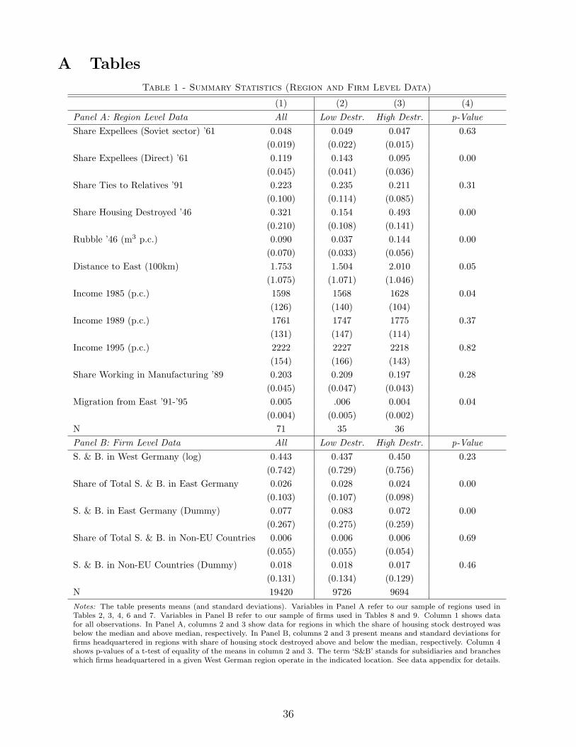
A Tables

Table 1 - Summary Statistics (Region and Firm Level Data)

(1) (2) (3) (4)Panel A: Region Level Data All Low Destr. High Destr. p-ValueShare Expellees (Soviet sector) ’61 0.048 0.049 0.047 0.63

(0.019) (0.022) (0.015)Share Expellees (Direct) ’61 0.119 0.143 0.095 0.00

(0.045) (0.041) (0.036)Share Ties to Relatives ’91 0.223 0.235 0.211 0.31

(0.100) (0.114) (0.085)Share Housing Destroyed ’46 0.321 0.154 0.493 0.00

(0.210) (0.108) (0.141)Rubble ’46 (m3 p.c.) 0.090 0.037 0.144 0.00

(0.070) (0.033) (0.056)Distance to East (100km) 1.753 1.504 2.010 0.05

(1.075) (1.071) (1.046)Income 1985 (p.c.) 1598 1568 1628 0.04

(126) (140) (104)Income 1989 (p.c.) 1761 1747 1775 0.37

(131) (147) (114)Income 1995 (p.c.) 2222 2227 2218 0.82

(154) (166) (143)Share Working in Manufacturing ’89 0.203 0.209 0.197 0.28

(0.045) (0.047) (0.043)Migration from East ’91-’95 0.005 .006 0.004 0.04

(0.004) (0.005) (0.002)N 71 35 36Panel B: Firm Level Data All Low Destr. High Destr. p-ValueS. & B. in West Germany (log) 0.443 0.437 0.450 0.23

(0.742) (0.729) (0.756)Share of Total S. & B. in East Germany 0.026 0.028 0.024 0.00

(0.103) (0.107) (0.098)S. & B. in East Germany (Dummy) 0.077 0.083 0.072 0.00

(0.267) (0.275) (0.259)Share of Total S. & B. in Non-EU Countries 0.006 0.006 0.006 0.69

(0.055) (0.055) (0.054)S. & B. in Non-EU Countries (Dummy) 0.018 0.018 0.017 0.46

(0.131) (0.134) (0.129)N 19420 9726 9694Notes: The table presents means (and standard deviations). Variables in Panel A refer to our sample of regions used inTables 2, 3, 4, 6 and 7. Variables in Panel B refer to our sample of firms used in Tables 8 and 9. Column 1 shows datafor all observations. In Panel A, columns 2 and 3 show data for regions in which the share of housing stock destroyed wasbelow the median and above median, respectively. In Panel B, columns 2 and 3 present means and standard deviations forfirms headquartered in regions with share of housing stock destroyed above and below the median, respectively. Column 4shows p-values of a t-test of equality of the means in column 2 and 3. The term ‘S&B’ stands for subsidiaries and brancheswhich firms headquartered in a given West German region operate in the indicated location. See data appendix for details.

36

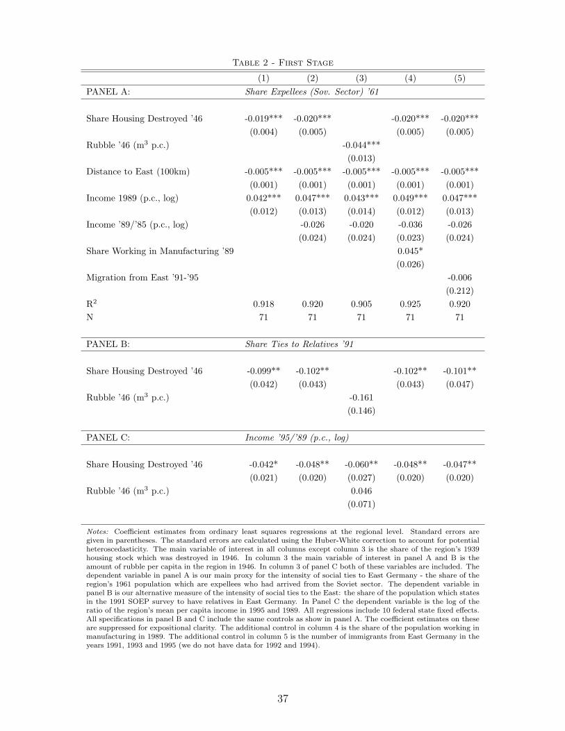
Table 2 - First Stage

(1) (2) (3) (4) (5)PANEL A: Share Expellees (Sov. Sector) ’61

Share Housing Destroyed ’46 -0.019*** -0.020*** -0.020*** -0.020***(0.004) (0.005) (0.005) (0.005)

Rubble ’46 (m3 p.c.) -0.044***(0.013)

Distance to East (100km) -0.005*** -0.005*** -0.005*** -0.005*** -0.005***(0.001) (0.001) (0.001) (0.001) (0.001)

Income 1989 (p.c., log) 0.042*** 0.047*** 0.043*** 0.049*** 0.047***(0.012) (0.013) (0.014) (0.012) (0.013)

Income ’89/’85 (p.c., log) -0.026 -0.020 -0.036 -0.026(0.024) (0.024) (0.023) (0.024)

Share Working in Manufacturing ’89 0.045*(0.026)

Migration from East ’91-’95 -0.006(0.212)

R2 0.918 0.920 0.905 0.925 0.920N 71 71 71 71 71

PANEL B: Share Ties to Relatives ’91

Share Housing Destroyed ’46 -0.099** -0.102** -0.102** -0.101**(0.042) (0.043) (0.043) (0.047)

Rubble ’46 (m3 p.c.) -0.161(0.146)

PANEL C: Income ’95/’89 (p.c., log)

Share Housing Destroyed ’46 -0.042* -0.048** -0.060** -0.048** -0.047**(0.021) (0.020) (0.027) (0.020) (0.020)

Rubble ’46 (m3 p.c.) 0.046(0.071)

Notes: Coefficient estimates from ordinary least squares regressions at the regional level. Standard errors aregiven in parentheses. The standard errors are calculated using the Huber-White correction to account for potentialheteroscedasticity. The main variable of interest in all columns except column 3 is the share of the region’s 1939housing stock which was destroyed in 1946. In column 3 the main variable of interest in panel A and B is theamount of rubble per capita in the region in 1946. In column 3 of panel C both of these variables are included. Thedependent variable in panel A is our main proxy for the intensity of social ties to East Germany - the share of theregion’s 1961 population which are expellees who had arrived from the Soviet sector. The dependent variable inpanel B is our alternative measure of the intensity of social ties to the East: the share of the population which statesin the 1991 SOEP survey to have relatives in East Germany. In Panel C the dependent variable is the log of theratio of the region’s mean per capita income in 1995 and 1989. All regressions include 10 federal state fixed effects.All specifications in panel B and C include the same controls as show in panel A. The coefficient estimates on theseare suppressed for expositional clarity. The additional control in column 4 is the share of the population working inmanufacturing in 1989. The additional control in column 5 is the number of immigrants from East Germany in theyears 1991, 1993 and 1995 (we do not have data for 1992 and 1994).

37

Table 3 - IV Estimation

(IV) (OLS) (IV)(1) (2) (3) (4) (5) (6)

Income ’95/’89 (p.c., log)

Share Expellees (Sov. S.) ’61 2.169** 1.963*** 2.442*** 2.453*** 2.428*** 2.366***(0.947) (0.574) (0.880) (0.877) (0.882) (0.878)

Distance to East (100km) 0.011** 0.008** 0.011** 0.011** 0.008** 0.011**(0.004) (0.003) (0.004) (0.004) (0.004) (0.004)

Income 1989 (p.c., log) -0.267*** -0.189*** -0.209*** -0.209*** -0.221*** -0.206***(0.068) (0.060) (0.060) (0.060) (0.059) (0.062)

Income ’89/’85 (p.c., log) -0.362*** -0.355*** -0.355*** -0.307*** -0.353***(0.083) (0.086) (0.086) (0.080) (0.087)

Share Working in Manufacturing ’89 -0.223**(0.097)

Migration from East ’91-’95 0.349(1.130)

R2 0.505 0.598 0.590 0.589 0.626 0.593N 71 71 71 71 71 71Instruments Housing - Housing Housing Housing Housing

& Rubble

Notes: The table reports coefficient estimates from instrumental variable regressions at the regional level in columns 1 and 3through 6. Column 2 reports results from an ordinary least squares regression. Standard errors are given in parentheses. Thestandard errors are calculated using the Huber-White correction to account for potential heteroscedasticity. The dependent variableis in all regressions the log of the ratio of mean per capita income in 1995 and 1989. The main variable of interest in all columnsis the share of the region’s 1961 population which are expellees who had arrived from the Soviet sector. In column 1, 3, 5 and 6we have instrumented for this with the share of the region’s 1939 housing stock which was destroyed in 1946. In column 4 we usethe amount of rubble per capita in 1946 as additional instrument. First stage results are shown in Table 2. All regressions controlfor a region’s distance to the former East German border and the log of mean per capita income in 1989. All regressions include10 federal state fixed effects. Columns 2-6 include the log of the ratio of mean per capita income in 1989 and 1985 as control.The regression shown in column 4 controls for the share working in manufacturing in 1989 and the regression shown in column 5controls for the number of regional immigrants from East Germany in the years 1991, 1993 and 1995 (we do not have data for 1992and 1994).

38

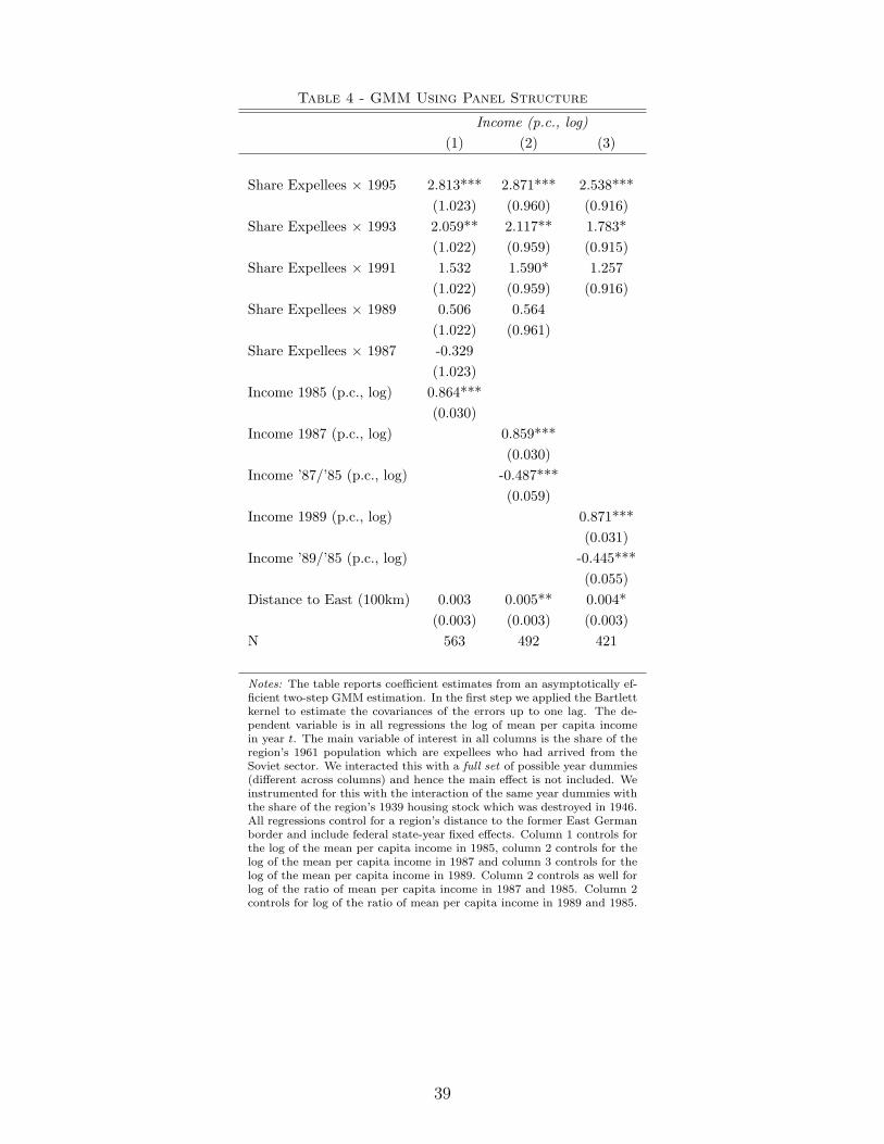
Table 4 - GMM Using Panel Structure

Income (p.c., log)(1) (2) (3)

Share Expellees × 1995 2.813*** 2.871*** 2.538***(1.023) (0.960) (0.916)

Share Expellees × 1993 2.059** 2.117** 1.783*(1.022) (0.959) (0.915)

Share Expellees × 1991 1.532 1.590* 1.257(1.022) (0.959) (0.916)

Share Expellees × 1989 0.506 0.564(1.022) (0.961)

Share Expellees × 1987 -0.329(1.023)

Income 1985 (p.c., log) 0.864***(0.030)

Income 1987 (p.c., log) 0.859***(0.030)

Income ’87/’85 (p.c., log) -0.487***(0.059)

Income 1989 (p.c., log) 0.871***(0.031)

Income ’89/’85 (p.c., log) -0.445***(0.055)

Distance to East (100km) 0.003 0.005** 0.004*(0.003) (0.003) (0.003)

N 563 492 421

Notes: The table reports coefficient estimates from an asymptotically ef-ficient two-step GMM estimation. In the first step we applied the Bartlettkernel to estimate the covariances of the errors up to one lag. The de-pendent variable is in all regressions the log of mean per capita incomein year t. The main variable of interest in all columns is the share of theregion’s 1961 population which are expellees who had arrived from theSoviet sector. We interacted this with a full set of possible year dummies(different across columns) and hence the main effect is not included. Weinstrumented for this with the interaction of the same year dummies withthe share of the region’s 1939 housing stock which was destroyed in 1946.All regressions control for a region’s distance to the former East Germanborder and include federal state-year fixed effects. Column 1 controls forthe log of the mean per capita income in 1985, column 2 controls for thelog of the mean per capita income in 1987 and column 3 controls for thelog of the mean per capita income in 1989. Column 2 controls as well forlog of the ratio of mean per capita income in 1987 and 1985. Column 2controls for log of the ratio of mean per capita income in 1989 and 1985.

39

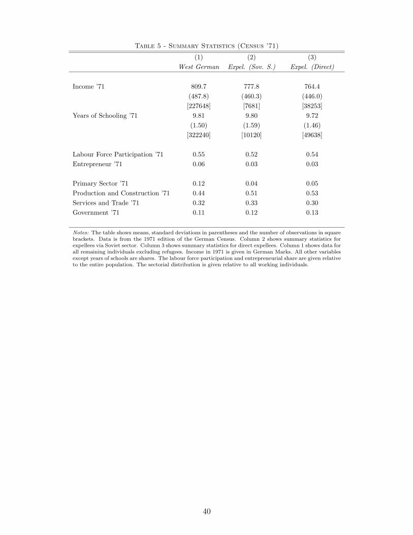
Table 5 - Summary Statistics (Census ’71)

(1) (2) (3)West German Expel. (Sov. S.) Expel. (Direct)

Income ’71 809.7 777.8 764.4(487.8) (460.3) (446.0)[227648] [7681] [38253]

Years of Schooling ’71 9.81 9.80 9.72(1.50) (1.59) (1.46)

[322240] [10120] [49638]

Labour Force Participation ’71 0.55 0.52 0.54Entrepreneur ’71 0.06 0.03 0.03

Primary Sector ’71 0.12 0.04 0.05Production and Construction ’71 0.44 0.51 0.53Services and Trade ’71 0.32 0.33 0.30Government ’71 0.11 0.12 0.13

Notes: The table shows means, standard deviations in parentheses and the number of observations in squarebrackets. Data is from the 1971 edition of the German Census. Column 2 shows summary statistics forexpellees via Soviet sector. Column 3 shows summary statistics for direct expellees. Column 1 shows data forall remaining individuals excluding refugees. Income in 1971 is given in German Marks. All other variablesexcept years of schools are shares. The labour force participation and entrepreneurial share are given relativeto the entire population. The sectorial distribution is given relative to all working individuals.

40

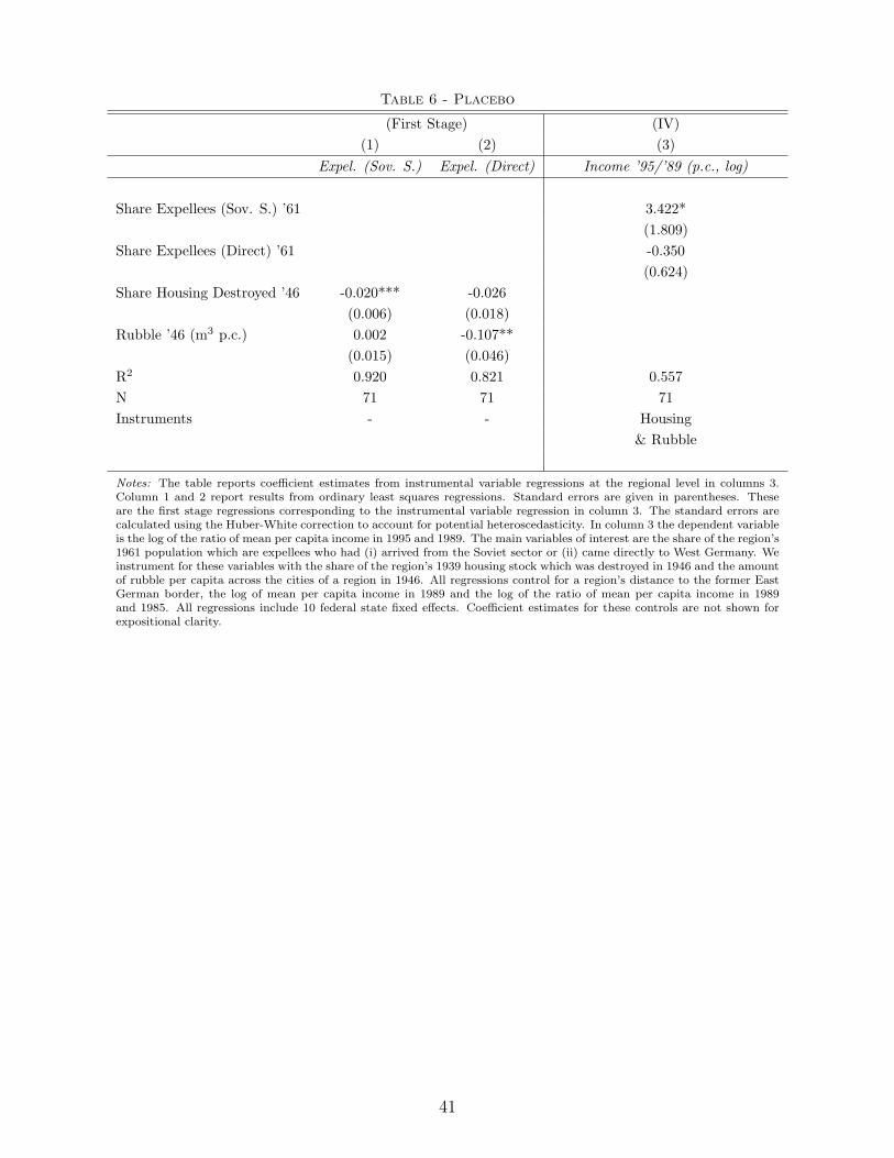
Table 6 - Placebo

(First Stage) (IV)(1) (2) (3)

Expel. (Sov. S.) Expel. (Direct) Income ’95/’89 (p.c., log)

Share Expellees (Sov. S.) ’61 3.422*(1.809)

Share Expellees (Direct) ’61 -0.350(0.624)

Share Housing Destroyed ’46 -0.020*** -0.026(0.006) (0.018)

Rubble ’46 (m3 p.c.) 0.002 -0.107**(0.015) (0.046)

R2 0.920 0.821 0.557N 71 71 71Instruments - - Housing

& Rubble

Notes: The table reports coefficient estimates from instrumental variable regressions at the regional level in columns 3.Column 1 and 2 report results from ordinary least squares regressions. Standard errors are given in parentheses. Theseare the first stage regressions corresponding to the instrumental variable regression in column 3. The standard errors arecalculated using the Huber-White correction to account for potential heteroscedasticity. In column 3 the dependent variableis the log of the ratio of mean per capita income in 1995 and 1989. The main variables of interest are the share of the region’s1961 population which are expellees who had (i) arrived from the Soviet sector or (ii) came directly to West Germany. Weinstrument for these variables with the share of the region’s 1939 housing stock which was destroyed in 1946 and the amountof rubble per capita across the cities of a region in 1946. All regressions control for a region’s distance to the former EastGerman border, the log of mean per capita income in 1989 and the log of the ratio of mean per capita income in 1989and 1985. All regressions include 10 federal state fixed effects. Coefficient estimates for these controls are not shown forexpositional clarity.

41

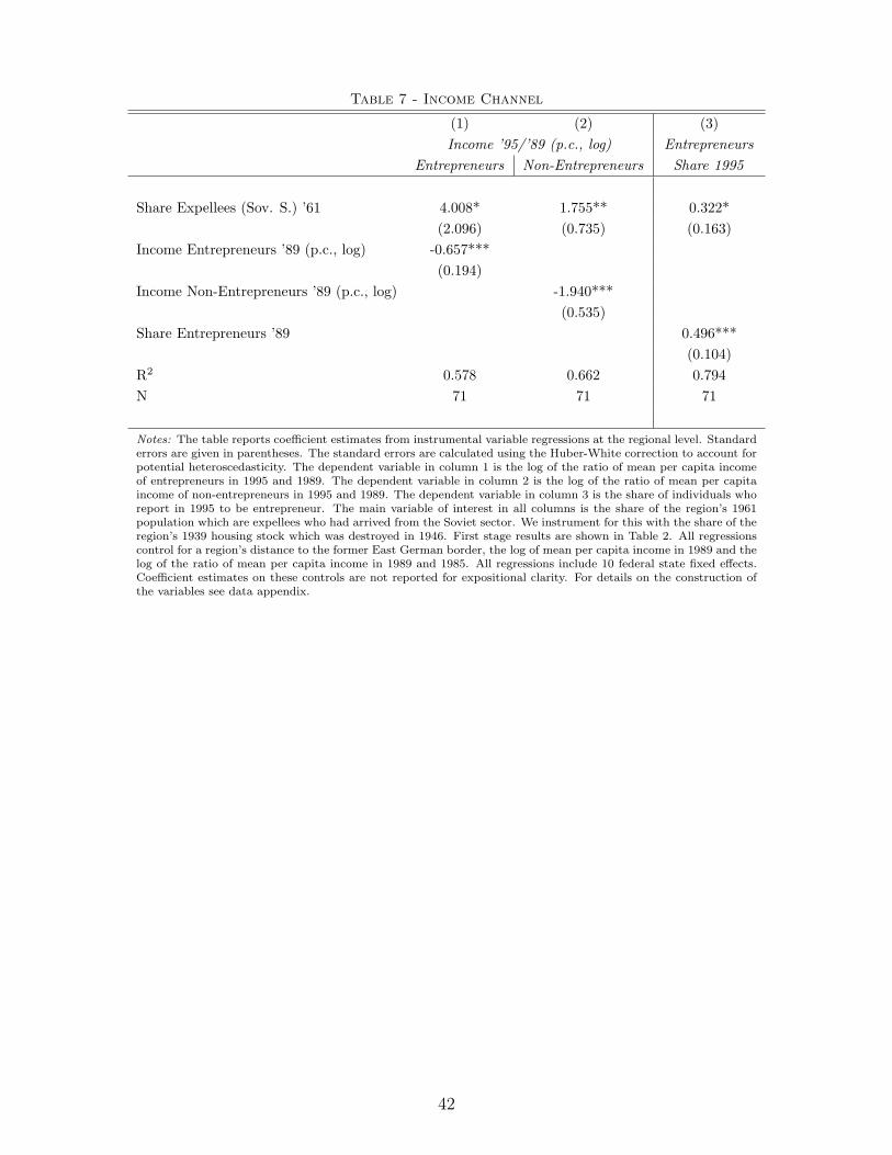
Table 7 - Income Channel

(1) (2) (3)Income ’95/’89 (p.c., log) Entrepreneurs

Entrepreneurs Non-Entrepreneurs Share 1995

Share Expellees (Sov. S.) ’61 4.008* 1.755** 0.322*(2.096) (0.735) (0.163)

Income Entrepreneurs ’89 (p.c., log) -0.657***(0.194)

Income Non-Entrepreneurs ’89 (p.c., log) -1.940***(0.535)

Share Entrepreneurs ’89 0.496***(0.104)

R2 0.578 0.662 0.794N 71 71 71

Notes: The table reports coefficient estimates from instrumental variable regressions at the regional level. Standarderrors are given in parentheses. The standard errors are calculated using the Huber-White correction to account forpotential heteroscedasticity. The dependent variable in column 1 is the log of the ratio of mean per capita incomeof entrepreneurs in 1995 and 1989. The dependent variable in column 2 is the log of the ratio of mean per capitaincome of non-entrepreneurs in 1995 and 1989. The dependent variable in column 3 is the share of individuals whoreport in 1995 to be entrepreneur. The main variable of interest in all columns is the share of the region’s 1961population which are expellees who had arrived from the Soviet sector. We instrument for this with the share of theregion’s 1939 housing stock which was destroyed in 1946. First stage results are shown in Table 2. All regressionscontrol for a region’s distance to the former East German border, the log of mean per capita income in 1989 and thelog of the ratio of mean per capita income in 1989 and 1985. All regressions include 10 federal state fixed effects.Coefficient estimates on these controls are not reported for expositional clarity. For details on the construction ofthe variables see data appendix.

42

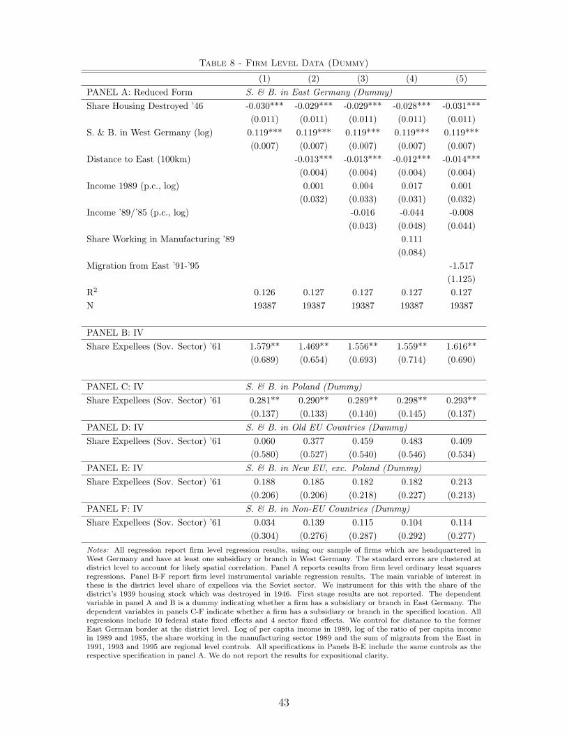
Table 8 - Firm Level Data (Dummy)

(1) (2) (3) (4) (5)PANEL A: Reduced Form S. & B. in East Germany (Dummy)Share Housing Destroyed ’46 -0.030*** -0.029*** -0.029*** -0.028*** -0.031***

(0.011) (0.011) (0.011) (0.011) (0.011)S. & B. in West Germany (log) 0.119*** 0.119*** 0.119*** 0.119*** 0.119***

(0.007) (0.007) (0.007) (0.007) (0.007)Distance to East (100km) -0.013*** -0.013*** -0.012*** -0.014***

(0.004) (0.004) (0.004) (0.004)Income 1989 (p.c., log) 0.001 0.004 0.017 0.001

(0.032) (0.033) (0.031) (0.032)Income ’89/’85 (p.c., log) -0.016 -0.044 -0.008

(0.043) (0.048) (0.044)Share Working in Manufacturing ’89 0.111

(0.084)Migration from East ’91-’95 -1.517

(1.125)R2 0.126 0.127 0.127 0.127 0.127N 19387 19387 19387 19387 19387

PANEL B: IVShare Expellees (Sov. Sector) ’61 1.579** 1.469** 1.556** 1.559** 1.616**

(0.689) (0.654) (0.693) (0.714) (0.690)

PANEL C: IV S. & B. in Poland (Dummy)Share Expellees (Sov. Sector) ’61 0.281** 0.290** 0.289** 0.298** 0.293**

(0.137) (0.133) (0.140) (0.145) (0.137)PANEL D: IV S. & B. in Old EU Countries (Dummy)Share Expellees (Sov. Sector) ’61 0.060 0.377 0.459 0.483 0.409

(0.580) (0.527) (0.540) (0.546) (0.534)PANEL E: IV S. & B. in New EU, exc. Poland (Dummy)Share Expellees (Sov. Sector) ’61 0.188 0.185 0.182 0.182 0.213

(0.206) (0.206) (0.218) (0.227) (0.213)PANEL F: IV S. & B. in Non-EU Countries (Dummy)Share Expellees (Sov. Sector) ’61 0.034 0.139 0.115 0.104 0.114

(0.304) (0.276) (0.287) (0.292) (0.277)Notes: All regression report firm level regression results, using our sample of firms which are headquartered inWest Germany and have at least one subsidiary or branch in West Germany. The standard errors are clustered atdistrict level to account for likely spatial correlation. Panel A reports results from firm level ordinary least squaresregressions. Panel B-F report firm level instrumental variable regression results. The main variable of interest inthese is the district level share of expellees via the Soviet sector. We instrument for this with the share of thedistrict’s 1939 housing stock which was destroyed in 1946. First stage results are not reported. The dependentvariable in panel A and B is a dummy indicating whether a firm has a subsidiary or branch in East Germany. Thedependent variables in panels C-F indicate whether a firm has a subsidiary or branch in the specified location. Allregressions include 10 federal state fixed effects and 4 sector fixed effects. We control for distance to the formerEast German border at the district level. Log of per capita income in 1989, log of the ratio of per capita incomein 1989 and 1985, the share working in the manufacturing sector 1989 and the sum of migrants from the East in1991, 1993 and 1995 are regional level controls. All specifications in Panels B-E include the same controls as therespective specification in panel A. We do not report the results for expositional clarity.

43

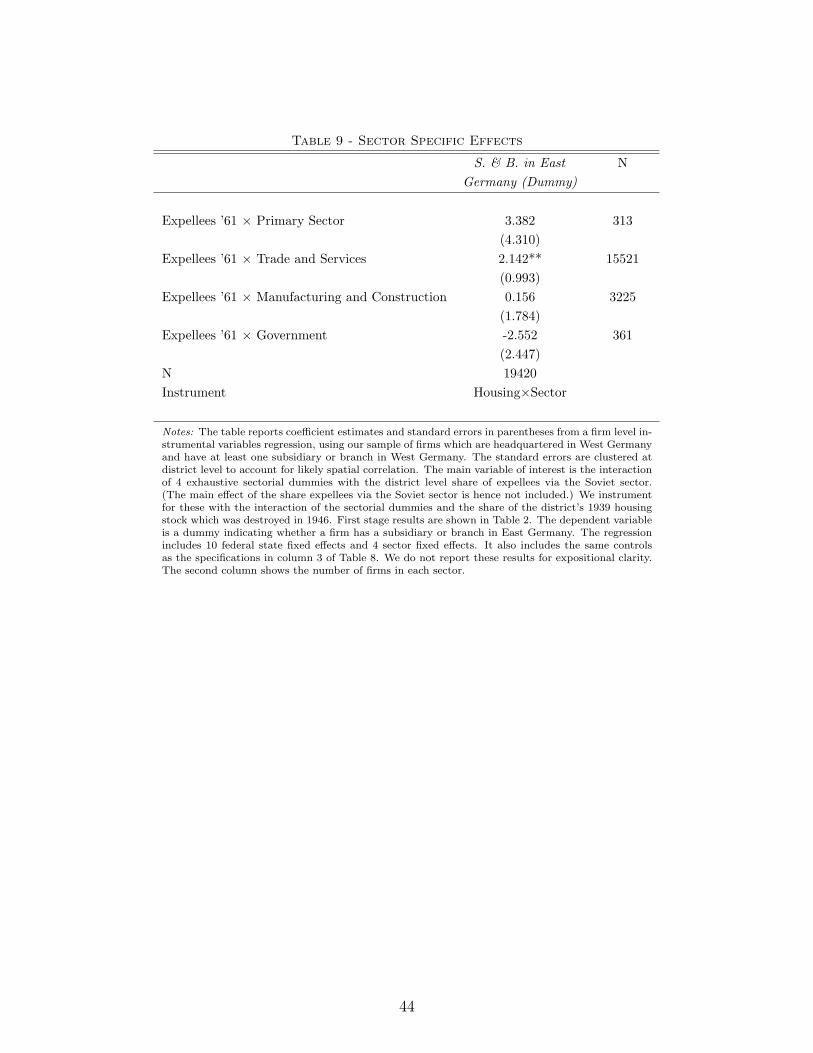
Table 9 - Sector Specific Effects

S. & B. in East NGermany (Dummy)

Expellees ’61 × Primary Sector 3.382 313(4.310)

Expellees ’61 × Trade and Services 2.142** 15521(0.993)

Expellees ’61 × Manufacturing and Construction 0.156 3225(1.784)

Expellees ’61 × Government -2.552 361(2.447)

N 19420Instrument Housing×Sector

Notes: The table reports coefficient estimates and standard errors in parentheses from a firm level in-strumental variables regression, using our sample of firms which are headquartered in West Germanyand have at least one subsidiary or branch in West Germany. The standard errors are clustered atdistrict level to account for likely spatial correlation. The main variable of interest is the interactionof 4 exhaustive sectorial dummies with the district level share of expellees via the Soviet sector.(The main effect of the share expellees via the Soviet sector is hence not included.) We instrumentfor these with the interaction of the sectorial dummies and the share of the district’s 1939 housingstock which was destroyed in 1946. First stage results are shown in Table 2. The dependent variableis a dummy indicating whether a firm has a subsidiary or branch in East Germany. The regressionincludes 10 federal state fixed effects and 4 sector fixed effects. It also includes the same controlsas the specifications in column 3 of Table 8. We do not report these results for expositional clarity.The second column shows the number of firms in each sector.

44

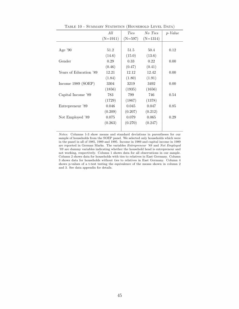
Table 10 - Summary Statistics (Household Level Data)

All Ties No Ties p-Value(N=1911) (N=597) (N=1314)

Age ’90 51.2 51.5 50.4 0.12(14.6) (15.0) (13.6)

Gender 0.29 0.33 0.22 0.00(0.46) (0.47) (0.41)

Years of Education ’89 12.21 12.12 12.42 0.00(1.84) (1.80) (1.91)

Income 1989 (SOEP) 3304 3219 3492 0.00(1856) (1935) (1656)

Capital Income ’89 783 799 746 0.54(1729) (1867) (1378)

Entrepreneur ’89 0.046 0.045 0.047 0.85(0.209) (0.207) (0.212)

Not Employed ’89 0.075 0.079 0.065 0.29(0.263) (0.270) (0.247)

Notes: Columns 1-3 show means and standard deviations in parentheses for oursample of households from the SOEP panel. We selected only households which werein the panel in all of 1985, 1989 and 1995. Income in 1989 and capital income in 1989are reported in German Marks. The variables Entrepreneur ’89 and Not Employed’89 are dummy variables indicating whether the household head is entrepreneur andnot working, respectively. Column 1 shows data for all observations in our sample.Column 2 shows data for households with ties to relatives in East Germany. Column3 shows data for households without ties to relatives in East Germany. Column 4shows p-values of a t-test testing the equivalence of the means shown in column 2and 3. See data appendix for details.

45

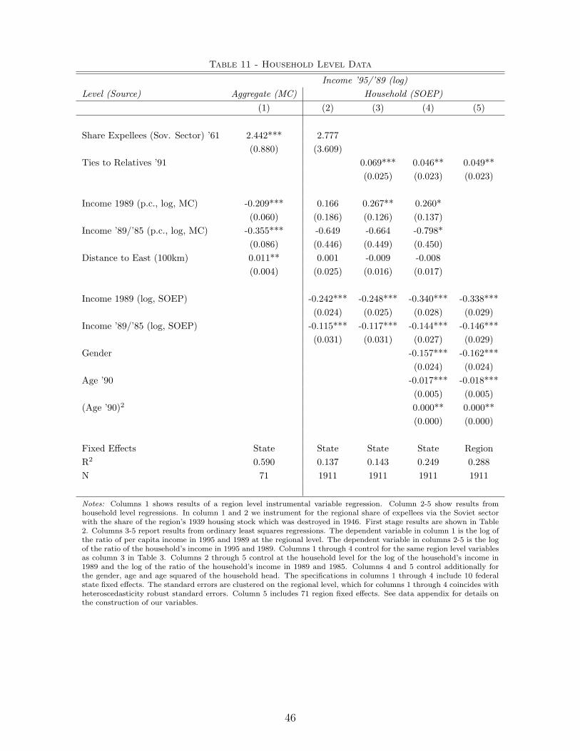
Table 11 - Household Level Data

Income ’95/’89 (log)Level (Source) Aggregate (MC) Household (SOEP)

(1) (2) (3) (4) (5)

Share Expellees (Sov. Sector) ’61 2.442*** 2.777(0.880) (3.609)

Ties to Relatives ’91 0.069*** 0.046** 0.049**(0.025) (0.023) (0.023)

Income 1989 (p.c., log, MC) -0.209*** 0.166 0.267** 0.260*(0.060) (0.186) (0.126) (0.137)

Income ’89/’85 (p.c., log, MC) -0.355*** -0.649 -0.664 -0.798*(0.086) (0.446) (0.449) (0.450)

Distance to East (100km) 0.011** 0.001 -0.009 -0.008(0.004) (0.025) (0.016) (0.017)

Income 1989 (log, SOEP) -0.242*** -0.248*** -0.340*** -0.338***(0.024) (0.025) (0.028) (0.029)

Income ’89/’85 (log, SOEP) -0.115*** -0.117*** -0.144*** -0.146***(0.031) (0.031) (0.027) (0.029)

Gender -0.157*** -0.162***(0.024) (0.024)

Age ’90 -0.017*** -0.018***(0.005) (0.005)

(Age ’90)2 0.000** 0.000**(0.000) (0.000)

Fixed Effects State State State State RegionR2 0.590 0.137 0.143 0.249 0.288N 71 1911 1911 1911 1911

Notes: Columns 1 shows results of a region level instrumental variable regression. Column 2-5 show results fromhousehold level regressions. In column 1 and 2 we instrument for the regional share of expellees via the Soviet sectorwith the share of the region’s 1939 housing stock which was destroyed in 1946. First stage results are shown in Table2. Columns 3-5 report results from ordinary least squares regressions. The dependent variable in column 1 is the log ofthe ratio of per capita income in 1995 and 1989 at the regional level. The dependent variable in columns 2-5 is the logof the ratio of the household’s income in 1995 and 1989. Columns 1 through 4 control for the same region level variablesas column 3 in Table 3. Columns 2 through 5 control at the household level for the log of the household’s income in1989 and the log of the ratio of the household’s income in 1989 and 1985. Columns 4 and 5 control additionally forthe gender, age and age squared of the household head. The specifications in columns 1 through 4 include 10 federalstate fixed effects. The standard errors are clustered on the regional level, which for columns 1 through 4 coincides withheteroscedasticity robust standard errors. Column 5 includes 71 region fixed effects. See data appendix for details onthe construction of our variables.

46

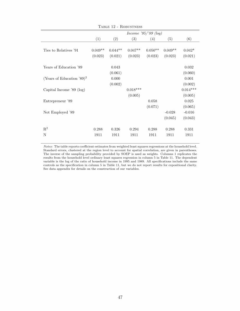
Table 12 - Robustness

Income ’95/’89 (log)(1) (2) (3) (4) (5) (6)

Ties to Relatives ’91 0.049** 0.044** 0.047** 0.050** 0.049** 0.042*(0.023) (0.021) (0.023) (0.023) (0.023) (0.021)

Years of Education ’89 0.043 0.032(0.061) (0.060)

(Years of Education ’89)2 0.000 0.001(0.002) (0.002)

Capital Income ’89 (log) 0.018*** 0.014***(0.005) (0.005)

Entrepreneur ’89 0.058 0.025(0.071) (0.065)

Not Employed ’89 -0.028 -0.016(0.045) (0.043)

R2 0.288 0.326 0.294 0.288 0.288 0.331N 1911 1911 1911 1911 1911 1911

Notes: The table reports coefficient estimates from weighted least squares regressions at the household level.Standard errors, clustered at the region level to account for spatial correlation, are given in parentheses.The inverse of the sampling probability provided by SOEP is used as weights. Columns 1 replicates theresults from the household level ordinary least squares regression in column 5 in Table 11. The dependentvariable is the log of the ratio of household income in 1995 and 1989. All specifications include the samecontrols as the specification in column 5 in Table 11, but we do not report results for expositional clarity.See data appendix for details on the construction of our variables.

47

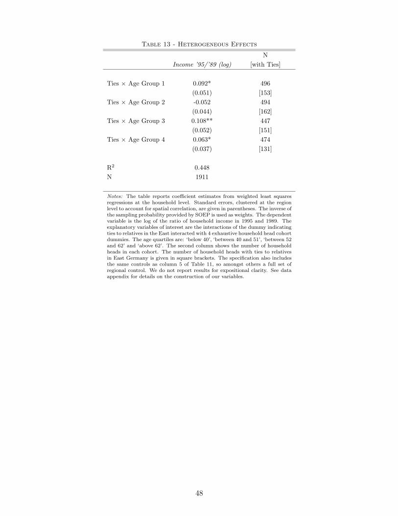
Table 13 - Heterogeneous Effects

NIncome ’95/’89 (log) [with Ties]

Ties × Age Group 1 0.092* 496(0.051) [153]

Ties × Age Group 2 -0.052 494(0.044) [162]

Ties × Age Group 3 0.108** 447(0.052) [151]

Ties × Age Group 4 0.063* 474(0.037) [131]

R2 0.448N 1911

Notes: The table reports coefficient estimates from weighted least squaresregressions at the household level. Standard errors, clustered at the regionlevel to account for spatial correlation, are given in parentheses. The inverse ofthe sampling probability provided by SOEP is used as weights. The dependentvariable is the log of the ratio of household income in 1995 and 1989. Theexplanatory variables of interest are the interactions of the dummy indicatingties to relatives in the East interacted with 4 exhaustive household head cohortdummies. The age quartiles are: ‘below 40’, ‘between 40 and 51’, ‘between 52and 62’ and ‘above 62’. The second column shows the number of householdheads in each cohort. The number of household heads with ties to relativesin East Germany is given in square brackets. The specification also includesthe same controls as column 5 of Table 11, so amongst others a full set ofregional control. We do not report results for expositional clarity. See dataappendix for details on the construction of our variables.

48

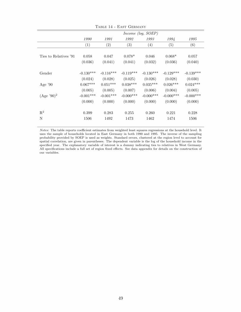
Table 14 - East Germany

Income (log, SOEP)1990 1991 1992 1993 1994 1995(1) (2) (3) (4) (5) (6)

Ties to Relatives ’91 0.058 0.047 0.078* 0.046 0.068* 0.057(0.036) (0.041) (0.041) (0.032) (0.036) (0.040)

Gender -0.130*** -0.116*** -0.119*** -0.130*** -0.129*** -0.139***(0.024) (0.028) (0.025) (0.026) (0.028) (0.030)

Age ’90 0.067*** 0.051*** 0.038*** 0.035*** 0.026*** 0.024***(0.005) (0.005) (0.007) (0.006) (0.004) (0.005)

(Age ’90)2 -0.001*** -0.001*** -0.000*** -0.000*** -0.000*** -0.000***(0.000) (0.000) (0.000) (0.000) (0.000) (0.000)

R2 0.399 0.283 0.255 0.260 0.221 0.228N 1506 1492 1473 1462 1474 1506

Notes: The table reports coefficient estimates from weighted least squares regressions at the household level. Ituses the sample of households located in East Germany in both 1990 and 1995. The inverse of the samplingprobability provided by SOEP is used as weights. Standard errors, clustered at the region level to account forspatial correlation, are given in parentheses. The dependent variable is the log of the household income in thespecified year. The explanatory variable of interest is a dummy indicating ties to relatives in West Germany.All specifications include a full set of region fixed effects. See data appendix for details on the construction ofour variables.

49

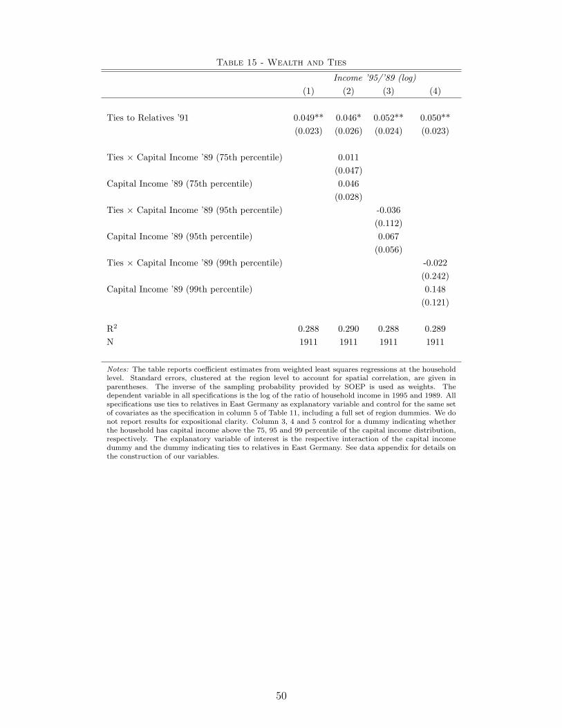
Table 15 - Wealth and Ties

Income ’95/’89 (log)(1) (2) (3) (4)

Ties to Relatives ’91 0.049** 0.046* 0.052** 0.050**(0.023) (0.026) (0.024) (0.023)

Ties × Capital Income ’89 (75th percentile) 0.011(0.047)

Capital Income ’89 (75th percentile) 0.046(0.028)

Ties × Capital Income ’89 (95th percentile) -0.036(0.112)

Capital Income ’89 (95th percentile) 0.067(0.056)

Ties × Capital Income ’89 (99th percentile) -0.022(0.242)

Capital Income ’89 (99th percentile) 0.148(0.121)

R2 0.288 0.290 0.288 0.289N 1911 1911 1911 1911

Notes: The table reports coefficient estimates from weighted least squares regressions at the householdlevel. Standard errors, clustered at the region level to account for spatial correlation, are given inparentheses. The inverse of the sampling probability provided by SOEP is used as weights. Thedependent variable in all specifications is the log of the ratio of household income in 1995 and 1989. Allspecifications use ties to relatives in East Germany as explanatory variable and control for the same setof covariates as the specification in column 5 of Table 11, including a full set of region dummies. We donot report results for expositional clarity. Column 3, 4 and 5 control for a dummy indicating whetherthe household has capital income above the 75, 95 and 99 percentile of the capital income distribution,respectively. The explanatory variable of interest is the respective interaction of the capital incomedummy and the dummy indicating ties to relatives in East Germany. See data appendix for details onthe construction of our variables.

50

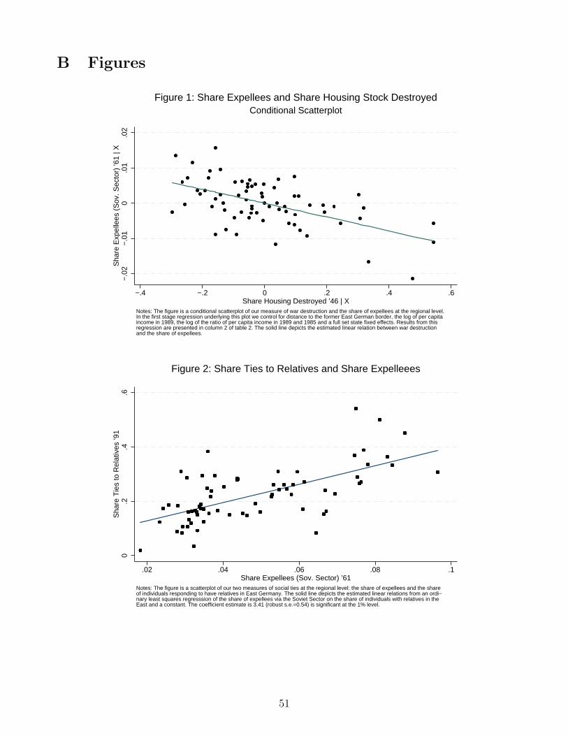
B Figures

−.0

2−

.01

0.0

1.0

2S

hare

Exp

elle

es (

Sov

. Sec

tor)

’61

| X

−.4 −.2 0 .2 .4 .6Share Housing Destroyed ’46 | X

Notes: The figure is a conditional scatterplot of our measure of war destruction and the share of expellees at the regional level.In the first stage regression underlying this plot we control for distance to the former East German border, the log of per capitaincome in 1989, the log of the ratio of per capita income in 1989 and 1985 and a full set state fixed effects. Results from thisregression are presented in column 2 of table 2. The solid line depicts the estimated linear relation between war destruction and the share of expellees.

Conditional Scatterplot

Figure 1: Share Expellees and Share Housing Stock Destroyed

0.2

.4.6

Sha

re T

ies

to R

elat

ives

’91

.02 .04 .06 .08 .1Share Expellees (Sov. Sector) ’61

Notes: The figure is a scatterplot of our two measures of social ties at the regional level: the share of expellees and the shareof individuals responding to have relatives in East Germany. The solid line depicts the estimated linear relations from an ordi−nary least squares regresssion of the share of expellees via the Soviet Sector on the share of individuals with relatives in the East and a constant. The coefficient estimate is 3.41 (robust s.e.=0.54) is significant at the 1% level.

Figure 2: Share Ties to Relatives and Share Expelleees

51

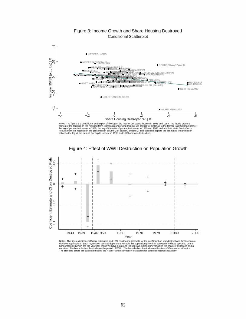
BONNSCHWARZWALD−BAAR−HEUBERGOSTWÜRTTEMBERG

GÖTTINGEN

NIEDERSACHSEN HB

BIELEFELD

OLDENBURG

NIEDERS. NORD

RHEIN−MAIN−TAUNUSBREMERHAVEN (NIEDERS.)

ALLGÄU

OBERPFALZ−NORDOSTHESSEN

HAGENOBERFRANKEN−WESTSÜDOSTOBERBAYERN

LÜNEBURG

WESTMITTELFRANKEN

MÖNCHENGLADBACH

MÜNSTER

OBERFRANKEN−WEST

BREMERHAVEN

MITTLERER OBERRHEINOSTHOLSTEIN

REGENSBURG

DONAU−ILLER (BAY.)

OBERFRANKEN−NORDBOCHUMSÜDLICHER OBERRHEINDÜSSELDORF

WUPPERTAL

MITTELHESSEN

TRIER

LANDSHUTESSEN

MITTLERER NECKAR

SCHLESWIG−H. HHDONAU−WALD

DORTMUND−SAUERLANDMITTELRHEIN−WESTERWALD

RHEINPFALZ

NECKAR−ALB

HAMBURGRHEINHESSEN−NAHE

AUGSBURG

UNTERER NECKAR

KREFELDWESTPFALZ

BRAUNSCHWEIG

MÜNCHEN

NORDHESSEN

AACHENDUISBURGHANNOVER

BREMEN

KÖLN

UNTERMAIN

MITTELHOLSTEIN

MAIN−RHÖN

DONAU−ILLER (BA−WÜ)

MITTELFRANKENBAYERISCHER UNTERMAINSTARKENBURG

FRANKENOSNABRÜCKSIEGEN

NORDSCHWARZWALD

WILHELMSHAVEN

OSTFRIESLAND

WÜRZBURGPADERBORN

−.1

−.0

50

.05

.1In

com

e ’9

5/’8

9 (p

.c.,

log)

| X

−.4 −.2 0 .2 .4 .6Share Housing Destroyed ’46 | X

Notes: The figure is a conditional scatterplot of the log of the ratio of per capita income in 1995 and 1989. The labels present names of the regions. In the reduced form regression underlying this plot we control for distance to the former East German border, the log of per capita income in 1989, the log of the ratio of per capita income in 1989 and 1985 and a full set state fixed effects. Results from this regression are presented in column 2 of panel C of table 2. The solid line depicts the estimated linear relation between the log of the ratio of per capita income in 1995 and 1989 and war destruction.

Conditional Scatterplot

Figure 3: Income Growth and Share Housing Destroyed

−.0

1−

.005

0.0

05C

oeffi

cien

t Est

imat

e an

d C

I on

Des

troy

ed F

lats

1933 1939 19461950 1960 1970 1979 1989 2000Year

Notes: The figure depicts coefficient estimates and 10% confidence intervals for the coefficient on war destructions for 9 separatecity level regressions. Each regression uses as dependent variable the population growth in between the dates specified on the horizontal axis (which are the years for which we have data) and includes as explanatory variables the share of expellees and aconstant. The black dashed line indicate the period of WWII. The blue dashed line indicates the time of German reunification. The standard errors are calculated using the Huber−White correction to account for potential heteroscedasticity.

Figure 4: Effect of WWII Destruction on Population Growth

52

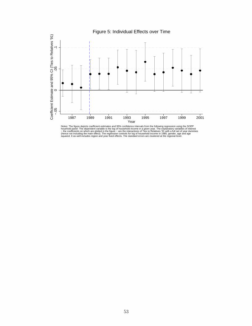
−.0

50

.05

.1C

oeffi

cien

t Est

imat

e an

d 95

% C

I (T

ies

to R

elat

ives

’91)

1987 1989 1991 1993 1995 1997 1999 2001Year

Notes: The figure depicts coefficient estimates and 95% confidence intervals from the following regression using the SOEPhouehold panel: The dependent variable is the log of household income in a given year. The explanatory variables of interest− the coefficients on which are plotted in the figure − are the interactions of Ties to Relatives ’91 with a full set of year dummies(hence not including the main effect). The regression controls for log of household income in 1985, gender, age and agesquared. It as well includes region and year fixed effects. The standard errors are clustered at the regional level.

Figure 5: Individual Effects over Time

53

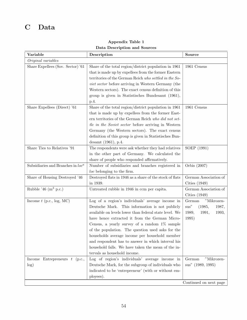
C Data

Appendix Table 1Data Description and Sources

Variable Description SourceOriginal variablesShare Expellees (Sov. Sector) ’61 Share of the total region/district population in 1961

that is made up by expellees from the former Easternterritories of the German Reich who settled in the So-viet sector before arriving in Western Germany (theWestern sectors). The exact census definition of thisgroup is given in Statistisches Bundesamt (1961),p.4.

1961 Census

Share Expellees (Direct) ’61 Share of the total region/district population in 1961that is made up by expellees from the former East-ern territories of the German Reich who did not set-tle in the Soviet sector before arriving in WesternGermany (the Western sectors). The exact censusdefinition of this group is given in Statistisches Bun-desamt (1961), p.4.

1961 Census

Share Ties to Relatives ’91 The respondents were ask whether they had relativesin the other part of Germany. We calculated theshare of people who responded affirmatively.

SOEP (1991)

Subsidiaries and Branches in loca Number of subsidiaries and branches registered inloc belonging to the firm.

Orbis (2007)

Share of Housing Destroyed ’46 Destroyed flats in 1946 as a share of the stock of flatsin 1939.

German Association ofCities (1949)

Rubble ’46 (m3 p.c.) Untreated rubble in 1946 in ccm per capita. German Association ofCities (1949)

Income t (p.c., log, MC) Log of a region’s individuals’ average income inDeutsche Mark. This information is not publiclyavailable on levels lower than federal state level. Wehave hence extracted it from the German Micro-Census, a yearly survey of a random 1% sampleof the population. The question used asks for thehouseholds average income per household memberand respondent has to answer in which interval hishousehold falls. We have taken the mean of the in-tervals as household income.

German ”Mikrozen-sus” (1985, 1987,1989, 1991, 1993,1995)

Income Entrepreneurs t (p.c.,log)

Log of region’s individuals’ average income inDeutsche Mark, for the subgroup of individuals whoindicated to be ‘entrepreneur’ (with or without em-ployees).

German ”Mikrozen-sus” (1989, 1995)

Continued on next page

54

Appendix Table 1 – continued from previous pageVariable Description SourceIncome Non-Entrepreneurs t

(p.c., log)Log of region’s individuals’ average income inDeutsche Mark, for the subgroup of individuals whoindicated to have an occupation other than being‘entrepreneur’ (with or without employees).

German ”Mikrozen-sus” (1989, 1995)

Share Entrepreneur t Regional share of individuals who indicate as occu-pation to be entrepreneur (with or without employ-ees).

German ”Mikrozen-sus” (1989)

Share Working in Manufacturing’89

Regional share of individuals who indicate to beworking in manufacturing.

German ”Mikrozen-sus” (1989)

Distance to East (100km) Closest distance from a region’s centre to the formerGDR’s border in 100 km.

- own calculations -

Migration from East ’91-’95 Surveyed individuals who migrated to the region inthe years 1991, 1993 and 1995 from East Germanyas a share the total surveyed population.

German ”Mikrozen-sus” (1991, 1993,1995)

Region The geocode of the ‘spacial ordering unit’, an ag-glomeration of on average 4.4 districts. This is thelowest level at which income data is made availablein the German Micro Census.

Ties to Relatives ’91 (Dummy) Dummy indicating whether household head or an-other person in the same household had relatives inthe other part of Germany in 1991.

German SOEP (1991)

Income t (log, SOEP) Log of income in German Mark of household headin year t .

German SOEP

Gender Gender of highest ranked individual in the householdfor whom income data exists. Usually this will bethe household head.

German SOEP (1990)

Age ’90 Age of household head in 1990. German SOEP (1990)Years of Education ’89 Years of education (including professional) of highest

ranked individual in the household for whom incomedata exists. Usually this will be the household head.

German SOEP (1990)

Capital Income ’89 Log of household capital income in 1989. German SOEP (1990)Occupation ’89 We aggregated the occupations given in the German

SOEP to the 8 categories ‘Not Employed’, ‘Pen-sioner’, ‘In Education/Military Service’, ‘Worker’,‘Farmer’, ‘White Collar’, ‘Entrepreneur’ and ‘CivilServant’.

German SOEP (1990)

Generated variablesIncome t1/t0 (p.c., log) Income t1 (p.c., log) - Income t0) (p.c., log).Share of Total Subsidiaries andBranches in loca

Number of subsidiaries and branches in loc overthe sum of this and the number of subsidiaries andbranches in West Germany.

Subsidiaries and Branches in loca

(Dummy)Dummy variable that indicates whether the firm op-erates at least one subsidiary or branch in loc.

Continued on next page

55

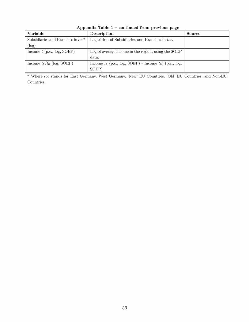
Appendix Table 1 – continued from previous pageVariable Description SourceSubsidiaries and Branches in loca

(log)Logarithm of Subsidiaries and Branches in loc.

Income t (p.c., log, SOEP) Log of average income in the region, using the SOEPdata.

Income t1/t0 (log, SOEP) Income t1 (p.c., log, SOEP) - Income t0) (p.c., log,SOEP)

a Where loc stands for East Germany, West Germany, ‘New’ EU Countries, ‘Old’ EU Countries, and Non-EUCountries.

56

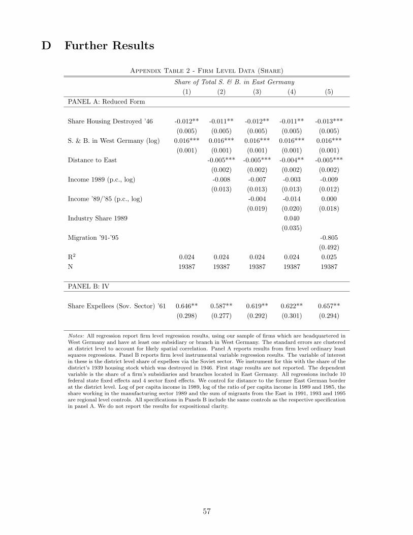
D Further Results

Appendix Table 2 - Firm Level Data (Share)

Share of Total S. & B. in East Germany(1) (2) (3) (4) (5)

PANEL A: Reduced Form

Share Housing Destroyed ’46 -0.012** -0.011** -0.012** -0.011** -0.013***(0.005) (0.005) (0.005) (0.005) (0.005)

S. & B. in West Germany (log) 0.016*** 0.016*** 0.016*** 0.016*** 0.016***(0.001) (0.001) (0.001) (0.001) (0.001)

Distance to East -0.005*** -0.005*** -0.004** -0.005***(0.002) (0.002) (0.002) (0.002)

Income 1989 (p.c., log) -0.008 -0.007 -0.003 -0.009(0.013) (0.013) (0.013) (0.012)

Income ’89/’85 (p.c., log) -0.004 -0.014 0.000(0.019) (0.020) (0.018)

Industry Share 1989 0.040(0.035)

Migration ’91-’95 -0.805(0.492)

R2 0.024 0.024 0.024 0.024 0.025N 19387 19387 19387 19387 19387

PANEL B: IV

Share Expellees (Sov. Sector) ’61 0.646** 0.587** 0.619** 0.622** 0.657**(0.298) (0.277) (0.292) (0.301) (0.294)

Notes: All regression report firm level regression results, using our sample of firms which are headquartered inWest Germany and have at least one subsidiary or branch in West Germany. The standard errors are clusteredat district level to account for likely spatial correlation. Panel A reports results from firm level ordinary leastsquares regressions. Panel B reports firm level instrumental variable regression results. The variable of interestin these is the district level share of expellees via the Soviet sector. We instrument for this with the share of thedistrict’s 1939 housing stock which was destroyed in 1946. First stage results are not reported. The dependentvariable is the share of a firm’s subsidiaries and branches located in East Germany. All regressions include 10federal state fixed effects and 4 sector fixed effects. We control for distance to the former East German borderat the district level. Log of per capita income in 1989, log of the ratio of per capita income in 1989 and 1985, theshare working in the manufacturing sector 1989 and the sum of migrants from the East in 1991, 1993 and 1995are regional level controls. All specifications in Panels B include the same controls as the respective specificationin panel A. We do not report the results for expositional clarity.

57

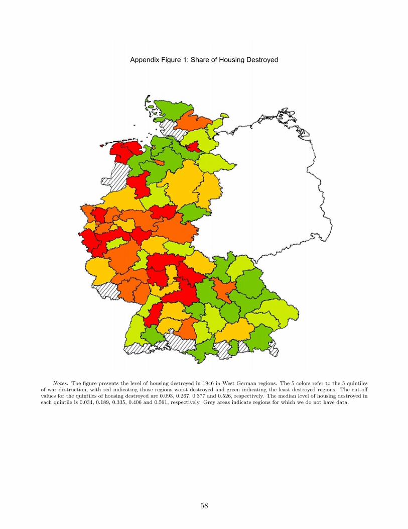
Appendix Figure 1: Share of Housing Destroyed

Notes: The figure presents the level of housing destroyed in 1946 in West German regions. The 5 colors refer to the 5 quintilesof war destruction, with red indicating those regions worst destroyed and green indicating the least destroyed regions. The cut-offvalues for the quintiles of housing destroyed are 0.093, 0.267, 0.377 and 0.526, respectively. The median level of housing destroyed ineach quintile is 0.034, 0.189, 0.335, 0.406 and 0.591, respectively. Grey areas indicate regions for which we do not have data.

58