THE ECONOMIC JOURNAL - CEMFIarellano/EJpapBAB.pdf* We wish to thank Daron Acemoglu, Alfonso Alba, Olivier Blanchard, Raquel Carrasco, Daniel Cohen, Jaume Garcı´a, Guido Imbens, Juan

THE ECONOMIC JOURNALA P R I L 2 0 0 2

The Economic Journal, 112 (April), 223–265. � Royal Economic Society 2002. Published by BlackwellPublishers, 108 Cowley Road, Oxford OX4 1JF, UK and 350 Main Street, Malden, MA 02148, USA.

UNEMPLOYMENT DURATION, BENEFIT DURATIONAND THE BUSINESS CYCLE*

Olympia Bover, Manuel Arellano and Samuel Bentolila

In this paper we study the effects of unemployment benefit duration and the business cycle onunemployment duration. We construct durations for individuals entering unemployment froma longitudinal sample of Spanish men in 1987–94. Estimated discrete hazard models indicatethat receipt of unemployment benefits significantly reduces the hazard of leaving unemploy-ment. At durations of three months, when the largest effects occur, the hazard for workerswithout benefits is twice as large as that for workers with benefits. Favourable business condi-tions increase the hazard of leaving unemployment. At sample-period magnitudes, this effect issignificantly smaller than that of benefit receipt.

Do unemployment benefits lead to longer unemployment spells? We would expectthis to be the case, since individuals will be more selective concerning job offersthe larger their out-of-work income. Moreover, under certain conditions, standardjob search theory predicts that increases in either the amount or the length ofunemployment benefit lengthens the duration of unemployment. Nevertheless,the effects of benefits on unemployment duration compound labour supply anddemand forces, so that their magnitude is an empirical issue; indeed one whichhas been debated for long in the economics literature.

In this paper we investigate the effect of receiving unemployment benefits onthe unemployment duration of male workers in Spain over the period 1987–94,using a longitudinal Labour Force Survey (LFS). We do so by comparing the exitrates of workers with and without benefits given unemployment duration, holdingdemographic and other variables constant. This is a meaningful exercise becauseour data have the fundamental virtue of providing exogenous variation acrossworkers in the receipt of benefits. This is an important difference between our dataand other data previously used in the empirical literature measuring effects ofbenefit entitlement. Often unemployed workers without benefits are a self-selectedminority with special characteristics (e.g. seasonal workers) and the effects ofbenefits are captured through marginal variation in the length of benefit entitle-ment.

* We wish to thank Daron Acemoglu, Alfonso Alba, Olivier Blanchard, Raquel Carrasco, DanielCohen, Jaume Garcıa, Guido Imbens, Juan Jimeno, Costas Meghir, Pedro Mira, Alfonso Novales, StevePischke, Enrique Sentana, Luis Toharia, Jose Vinals and three anonymous referees for usefulcomments. Cristina Barcelo, Raquel Carrasco and Francisco de Castro provided very helpful researchassistance. Any remaining errors are our own.

[ 223 ]

On the contrary, in our data, almost one-half of workers enter unemploymentwithout benefits. Moreover, the benefit–non-benefit division is close to a randomassignment resulting from the Spanish labour market reform of 1984. This reformcreated a country-wide natural experiment by producing a new type of unem-ployed worker without any benefits at all, that co-existed with otherwise similarworkers enjoying generous benefit entitlements.

Before 1984, the use of fixed-term contracts was restricted by law to certainactivities (like seasonal jobs or other temporary activities) and the only contractsavailable to firms for regular jobs were open-ended contracts with high firing costs.After the reform of 1984, firms were allowed to hire workers on fixed-term (e.g.three-month) contracts, with low or no firing costs, for any kind of activity. Themain restriction was that these contracts could only be renewed for a certainnumber of times, after which the temporary worker was either hired permanentlyon the old type of contract or dismissed.

At the time of the reform, the unemployment rate was over 20%. From then on,most new hirings were under low-cost fixed-term contracts, and temporary workerswere typically dismissed at the end of the maximum contract length, to avoidtransfer to the high-cost permanent contracts. Thus, the typical pre-sample jobhistory of a prime-age male entering unemployment without benefits in oursample would be a sequence of short-term temporary contracts starting at somepoint after the 1984 reform, itself preceded by a permanent job that had ended,often due to a collective dismissal. The number of collective dismissals reached apeak in 1985, before the beginning of our sample, and a new peak in 1993, towardsthe end of our sample. So, both before and during our sample period, there wereintervals of intense destruction of permanent jobs, that for the individuals con-cerned were followed by the start of a sequence of temporary jobs.

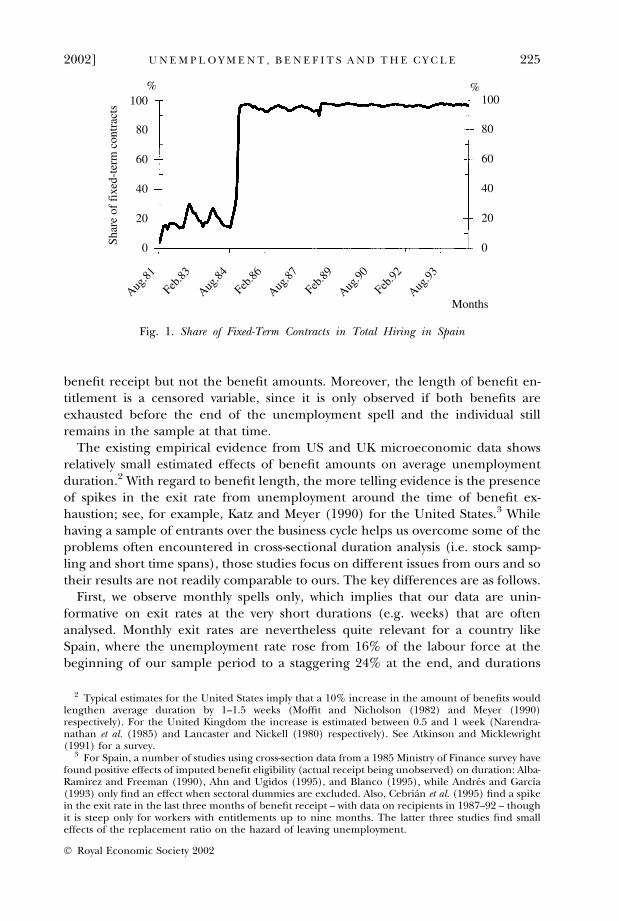
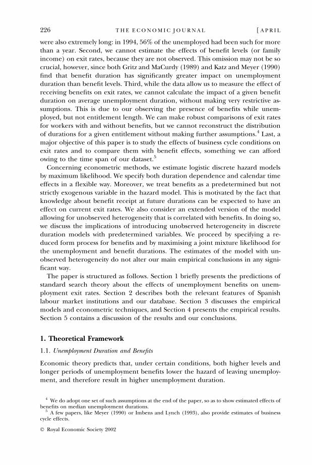
The jobs available to the unemployed in our sample were essentially fixed-termonly, regardless of whether they were receiving benefits, or whether their previousjob was temporary or permanent. Fig. 1 shows the gap between the pre- and post-reform shares of hirings under fixed-term contracts. Most prime-age workers inour sample must have held and lost a permanent job in their labour history. As aresult, employers would not view workers with more unstable job histories as beingless reliable than those with more stable histories. In a way, in this paper we arecomparing the (benefit covered) spell following the loss of a permanent job withsubsequent (non-covered) spells in between temporary jobs.1

Other relevant features of our data are as follows. First, the data set is large,which allows us to concentrate on unemployment entrants, whose information weexpect to be more reliable than retrospective information. Second, we observeindividuals’ labour market status for up to six consecutive quarters, so that a largeproportion of unemployment spells are not censored. Third, our sample periodspans a full business cycle of the Spanish economy, enabling us to take into ac-count changes in aggregate conditions. As a drawback, we observe unemployment

1 However, if the absence of benefits were associated with particular characteristics that made workersless employable, we would expect this to cause a downward bias in the measured effect of benefits onexit rates. For this reason, we also consider a version of the estimated model which allows forunobserved heterogeneity that is correlated with benefits.

224 [ A P R I LT H E E C O N O M I C J O U R N A L

� Royal Economic Society 2002

benefit receipt but not the benefit amounts. Moreover, the length of benefit en-titlement is a censored variable, since it is only observed if both benefits areexhausted before the end of the unemployment spell and the individual stillremains in the sample at that time.

The existing empirical evidence from US and UK microeconomic data showsrelatively small estimated effects of benefit amounts on average unemploymentduration.2 With regard to benefit length, the more telling evidence is the presenceof spikes in the exit rate from unemployment around the time of benefit ex-haustion; see, for example, Katz and Meyer (1990) for the United States.3 Whilehaving a sample of entrants over the business cycle helps us overcome some of theproblems often encountered in cross-sectional duration analysis (i.e. stock samp-ling and short time spans), those studies focus on different issues from ours and sotheir results are not readily comparable to ours. The key differences are as follows.

First, we observe monthly spells only, which implies that our data are unin-formative on exit rates at the very short durations (e.g. weeks) that are oftenanalysed. Monthly exit rates are nevertheless quite relevant for a country likeSpain, where the unemployment rate rose from 16% of the labour force at thebeginning of our sample period to a staggering 24% at the end, and durations

Shar

e of

fix

ed-t

erm

con

trac

ts100

80

60

40

20

0

100

80

60

40

20

0

Aug.93

Feb.92

Feb.89

Aug.90

Aug.87

Feb.86

Aug.84

Feb.83

Aug.81

Months

% %

Fig. 1. Share of Fixed-Term Contracts in Total Hiring in Spain

2 Typical estimates for the United States imply that a 10% increase in the amount of benefits wouldlengthen average duration by 1–1.5 weeks (Moffit and Nicholson (1982) and Meyer (1990)respectively). For the United Kingdom the increase is estimated between 0.5 and 1 week (Narendra-nathan et al. (1985) and Lancaster and Nickell (1980) respectively). See Atkinson and Micklewright(1991) for a survey.

3 For Spain, a number of studies using cross-section data from a 1985 Ministry of Finance survey havefound positive effects of imputed benefit eligibility (actual receipt being unobserved) on duration: Alba-Ramirez and Freeman (1990), Ahn and Ugidos (1995), and Blanco (1995), while Andres and Garcıa(1993) only find an effect when sectoral dummies are excluded. Also, Cebrian et al. (1995) find a spikein the exit rate in the last three months of benefit receipt – with data on recipients in 1987–92 – thoughit is steep only for workers with entitlements up to nine months. The latter three studies find smalleffects of the replacement ratio on the hazard of leaving unemployment.

2002] 225U N E M P L O Y M E N T , B E N E F I T S A N D T H E C Y C L E


were also extremely long: in 1994, 56% of the unemployed had been such for morethan a year. Second, we cannot estimate the effects of benefit levels (or familyincome) on exit rates, because they are not observed. This omission may not be socrucial, however, since both Gritz and MaCurdy (1989) and Katz and Meyer (1990)find that benefit duration has significantly greater impact on unemploymentduration than benefit levels. Third, while the data allow us to measure the effect ofreceiving benefits on exit rates, we cannot calculate the impact of a given benefitduration on average unemployment duration, without making very restrictive as-sumptions. This is due to our observing the presence of benefits while unem-ployed, but not entitlement length. We can make robust comparisons of exit ratesfor workers with and without benefits, but we cannot reconstruct the distributionof durations for a given entitlement without making further assumptions.4 Last, amajor objective of this paper is to study the effects of business cycle conditions onexit rates and to compare them with benefit effects, something we can affordowing to the time span of our dataset.5

Concerning econometric methods, we estimate logistic discrete hazard modelsby maximum likelihood. We specify both duration dependence and calendar timeeffects in a flexible way. Moreover, we treat benefits as a predetermined but notstrictly exogenous variable in the hazard model. This is motivated by the fact thatknowledge about benefit receipt at future durations can be expected to have aneffect on current exit rates. We also consider an extended version of the modelallowing for unobserved heterogeneity that is correlated with benefits. In doing so,we discuss the implications of introducing unobserved heterogeneity in discreteduration models with predetermined variables. We proceed by specifying a re-duced form process for benefits and by maximising a joint mixture likelihood forthe unemployment and benefit durations. The estimates of the model with un-observed heterogeneity do not alter our main empirical conclusions in any signi-ficant way.

The paper is structured as follows. Section 1 briefly presents the predictions ofstandard search theory about the effects of unemployment benefits on unem-ployment exit rates. Section 2 describes both the relevant features of Spanishlabour market institutions and our database. Section 3 discusses the empiricalmodels and econometric techniques, and Section 4 presents the empirical results.Section 5 contains a discussion of the results and our conclusions.

1. Theoretical Framework

1.1. Unemployment Duration and Benefits

Economic theory predicts that, under certain conditions, both higher levels andlonger periods of unemployment benefits lower the hazard of leaving unemploy-ment, and therefore result in higher unemployment duration.

4 We do adopt one set of such assumptions at the end of the paper, so as to show estimated effects ofbenefits on median unemployment durations.

5 A few papers, like Meyer (1990) or Imbens and Lynch (1993), also provide estimates of businesscycle effects.



The standard framework for analysing this issue is well known, as contained forexample in Mortensen (1977). The representative worker is assumed to maximisethe present value of his lifetime utility, which depends on income and leisure.Income when employed is equal to the wage, and to benefits when unemployed.Benefits are received as long as the worker has been laid off from a job and has notreached the maximum benefit duration (which depends on past employmenthistory). There is a stationary distribution of wage offers (jobs) and workers’ searchactivity is represented as random draws from that distribution. The probability ofleaving unemployment is the product of the probability of receiving an offer timesthe probability of accepting it. It is affected, among other things, by the worker’sdecision variables: search intensity and the reservation wage. On the one hand, theprobability of receiving an offer is proportional to the intensity of search. On theother hand, the worker’s optimal decision rule is to accept any wage offer above acertain reservation wage level.

Three key results concerning benefits emerge in this set-up. First, as exhaustionof benefits draws nearer, search intensity rises and the reservation wage falls, so thatthe hazard increases. Second, when benefits are exhausted, the hazard rate jumpsto a higher level (as long as income and leisure are strict complements in utility),remaining constant thereafter. Third, an increase in the amount or the maximumduration of unemployment benefits raises the opportunity cost of search, therebyleading to a reduction in the hazard. This disincentive effect of benefits may becountered by an entitlement effect: an increase in benefits increases the expectedutility from future, as opposed to current, unemployment spells with benefits.Thus, for a currently unemployed worker without benefits, an increase in thebenefit level or duration raises the exit rate from unemployment (i.e. employmentbecomes more valuable because it gives right to now-enhanced future benefits).Since future events are discounted for both uncertainty and time preferencereasons, we expect this to be a second-order effect for workers with benefits.

Later work has relaxed some of the assumptions in the standard model des-cribed above, leading to qualifications of the predictions regarding benefits(Atkinson and Micklewrigh, 1991). For example, receipt of unemployment bene-fits may permit an increase in the resources devoted to search by liquidity con-strained individuals, thereby leading to increased hazards. Therefore theprediction of a disincentive effect of benefits may be partially or totally offset forcertain individuals or periods by entitlement or other effects, and assessing thisbecomes an empirical question.

1.2. Duration, the Business Cycle, and Hysteresis

Search theory does not provide an unambiguous prediction on the sign of therelationship between the business cycle and unemployment duration. Highergrowth raises the probability of receiving a job offer, but it also tends to increasereservation wages.6 Empirical work has not resolved the issue either. For example,

6 However, Burdett (1981) shows that a sufficient condition for higher job availability reducingexpected unemployment duration is a ‘log-concave’ probability density function of wage offers.



with US data, Meyer (1990) finds that a higher state unemployment rate raises thehazard rates of unemployment benefit claimants, while Imbens and Lynch (1993)find that a higher local unemployment rate lowers the hazard rates of youngunemployed workers. The latter paper is one of the few that uses a long periodsample. Thus, firmer conclusions may be reached as more work is done on longersamples, like the one exploited in this paper.

Business cycle effects on individual unemployment duration are typically cap-tured in empirical work by variables like GDP growth or the unemployment rate(in levels and/or rates of change). Recent research has pointed out a new channelthrough which the change in unemployment would affect unemployment dura-tion, the so-called hysteresis effects. An increasing unemployment rate may reducea worker’s chances of re-employment more the longer his duration is if, as sug-gested by Layard et al. (1991, p. 365), it raises the share of recently unemployedworkers in the total pool of the unemployed and these workers are more attractiveto employers than the longer-term unemployed. This ranking behaviour of firms,proposed by Blanchard and Diamond (1994), could arise, for example, if humancapital loss increases with unemployment duration. We explore these issuesempirically for our sample of Spanish men.

2. Institutional Features and Data Description

2.1. Institutional Features

2.1.1. The Unemployment Benefit System in Spain. As in most European countries,unemployment benefits in Spain are of two types (details and a calendar of re-forms appear in Appendix 1, Tables A1–3). The unemployment insurance system(UI, Sistema contributivo) pays benefits to workers who have previously contributedwhen employed. They must have been dismissed from a job held at least for oneyear. The replacement ratio is currently equal to 70% of the previous wage duringthe first six months of unemployment and 60% thereafter, subject to a floor of75% of the minimum wage and to ceilings related to the number of dependants.Benefit duration is equal to one-third of the accumulated job tenure over someyears prior to unemployment, with a maximum duration of two years. The system’sgenerosity was reduced in 1992 and again in 1993.

The unemployment assistance system (UA, Sistema asistencial) grants supple-mentary income to workers who have exhausted UI benefits or who do not qualifyfor receiving them, with dependants, and whose average family income is below75% of the minimum wage. It pays precisely that amount, for up to two years. From1989 onwards, more generous conditions were granted to workers aged 45 or older,and benefits were extended until retirement age for workers aged 52 or older whoqualify for retirement except for their age. The system was made more generous in1992, but less generous in 1993. Last, there are special UA benefits for temporaryagricultural workers in the Southern regions of Andalucıa and Extremadura.Workers receive 75% of the minimum wage for 90–300 days within the year –depending on their age and number of dependants – provided they have beenemployed for at least 40 days (20 days if they were in the system already in 1983).



Going beyond the institutional setting, the actual coverage of unemploymentbenefits has increased in our sample period, from 35% of the unemployed in 1987to 55% in 1993, with a trend decline in the share of UI in the total, from 54% to50% over the same period (Toharia, 1997). For the population we analyse in thispaper, men between 20 and 64 years old, the coverage is larger and the proportionof workers on UI is slightly lower (for instance around 67% and 48%, respectively,for the 20–59 year-old group).

We have no direct information on the level of income enjoyed by the unem-ployed. We can nevertheless provide some related, aggregate information from theLabour Force Survey. In 1987:II, the first period in the sample we use below, 21%of households had at least one member unemployed and, in 7% of them, allmembers were unemployed. As to heads of household, they represented 22% ofthe unemployed, 4.5% of the unemployed were heads of households in which noother member was employed, and 5.7% of the unemployed were heads ofhouseholds in which no other member was receiving labour income (i.e. was eitheremployed, receiving benefits or receiving a pension).

2.1.2. Fixed-term Labour Contracts. An important institutional change affected un-employment duration in Spain within our sample period. The Spanish labourmarket reform of 1984 allowed fixed-term contracts to be used for any kind ofactivity, temporary or otherwise. They could be signed for six months (one year,since April 1992) up to three years. They entailed lower severance pay than per-manent contracts: nil, for some contract types, and 12 days of wages per year ofservice for other types, as opposed to 20 days if a permanent employee’s dismissalis either not challenged or else ruled fair in court, and to 45 days if ruled unfair.This labour reform caused swift increases in the share of fixed-term contracts inhiring, as shown in Fig. 1, and in the temporary employment rate (as a share ofemployees), which rose from 15% in 1987 to 34% in 1994. The latter rate is slightlylower among men (32% in 1994), higher among youth (58% for those aged20–29), and higher in agriculture and construction (around 58%) than inmanufacturing and services (around 28%). A direct consequence of this changehas been an increase in labour turnover rates. We estimate the impact oftemporary employment on unemployment outflow rates in Section 4.

2.2. The Data

The data we use come from the rotating panel of the Spanish Labour Force Survey(Encuesta de Poblacion Activa: Estadıstica de Flujos, EPA). The EPA is conducted everyquarter on all members of around 60,000 households. One sixth of the sample isrenewed quarterly; hence we can observe the labour market situation of an indi-vidual for up to six quarters. Some retrospective questions such as, for example, howlong the individual has been in the current job or looking for a job, are also asked.

The EPA started in its current form in 1987:II and we use the waves up to1994:III. These 30 quarters span a complete cycle of the Spanish economy. Thisdata set therefore has two important features. First, we can observe entrants into



unemployment, whose information we expect to be more reliable than retro-spective information. Second, we observe them over an extended period of time.This allows us to study the influence of personal characteristics, in particular ofbenefit duration, taking into account changes in aggregate conditions, so that wecan assess the relative importance of these factors.

The unemployed are asked each quarter whether they are receiving any un-employment benefits (without distinguishing between UI and UA). From theiranswers, we construct a duration of benefits variable, which is a censored entitle-ment to benefits variable since it only coincides with entitlement for workers withunemployment duration longer than benefit duration. We cannot construct ac-curate estimates of benefit entitlement duration from our data set. Contributorybenefit entitlement depends on accumulated job tenure over the 6 years prior tobecoming unemployed (4 years, before 1992), but the EPA provides informationonly about tenure in the latest job, which would be a poor guide to benefit en-titlement. Morever, entitlement to UA benefits depends on a mix of tenure, ageand family characteristics, so that estimates of benefit entitlement duration wouldbe very noisy. There is no information on benefit amounts, and these cannot beimputed either, because no wage information is available in the EPA.

In contrast to the cross-sectional EPA, the rotating panel – as currently released– only includes individuals over 16 years of age and does not provide informationon region of residence or family situation, except for marital and head-of-house-hold status. Given this fact, we focus on men, since for understanding marriedwomen’s behaviour it is particularly important to know the labour market situationof their husband and the number and age of their children. We also exclude fromour sample men aged 16 to 19 years old, given the instability of their attachment tothe labour market, and men aged 65 or older, due to the importance of transitionsto retirement at those ages. This leaves us with men aged 20 to 64.7

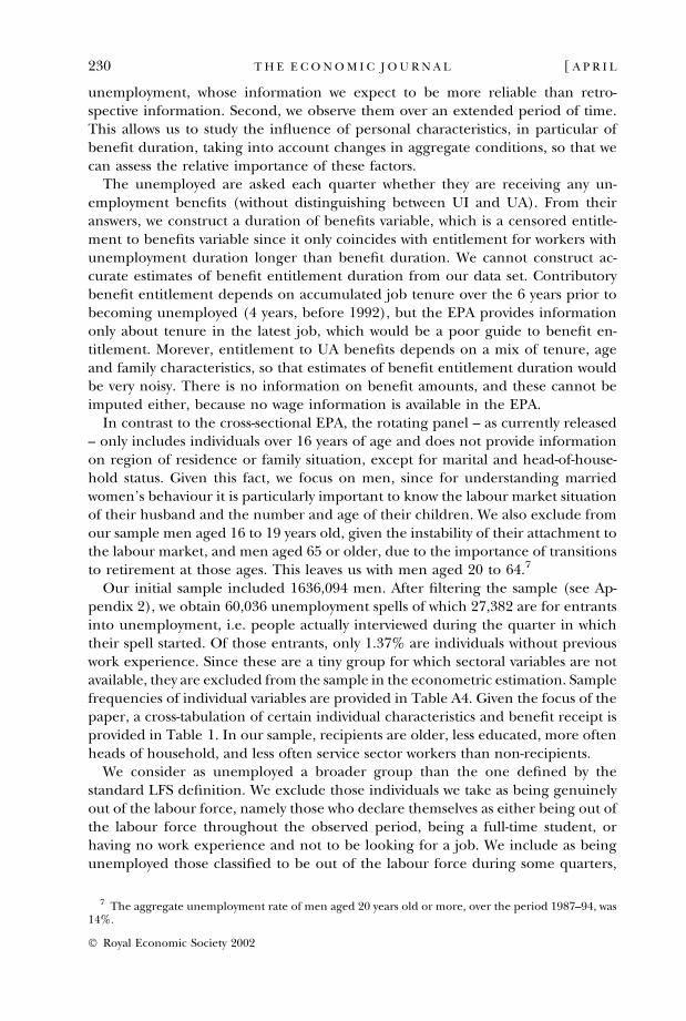
Our initial sample included 1636,094 men. After filtering the sample (see Ap-pendix 2), we obtain 60,036 unemployment spells of which 27,382 are for entrantsinto unemployment, i.e. people actually interviewed during the quarter in whichtheir spell started. Of those entrants, only 1.37% are individuals without previouswork experience. Since these are a tiny group for which sectoral variables are notavailable, they are excluded from the sample in the econometric estimation. Samplefrequencies of individual variables are provided in Table A4. Given the focus of thepaper, a cross-tabulation of certain individual characteristics and benefit receipt isprovided in Table 1. In our sample, recipients are older, less educated, more oftenheads of household, and less often service sector workers than non-recipients.

We consider as unemployed a broader group than the one defined by thestandard LFS definition. We exclude those individuals we take as being genuinelyout of the labour force, namely those who declare themselves as either being out ofthe labour force throughout the observed period, being a full-time student, orhaving no work experience and not to be looking for a job. We include as beingunemployed those classified to be out of the labour force during some quarters,

7 The aggregate unemployment rate of men aged 20 years old or more, over the period 1987–94, was14%.



which is not unreasonable having excluded women. Thus the transitions we look atare always from unemployment (or non-employment) to employment, rather thanto non-participation.

2.3. A First Look at Empirical Hazards, the Business Cycle, and Benefits

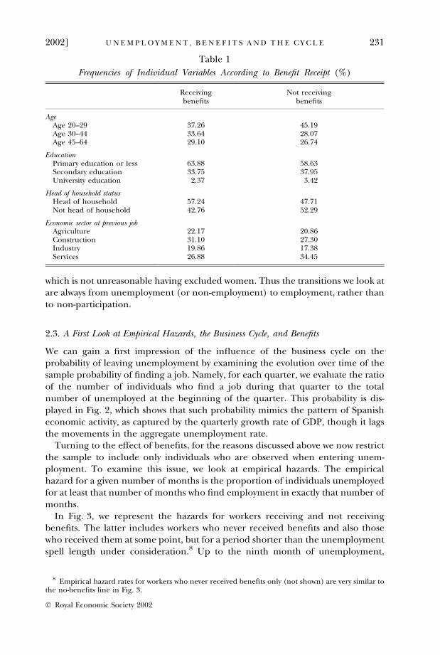
We can gain a first impression of the influence of the business cycle on theprobability of leaving unemployment by examining the evolution over time of thesample probability of finding a job. Namely, for each quarter, we evaluate the ratioof the number of individuals who find a job during that quarter to the totalnumber of unemployed at the beginning of the quarter. This probability is dis-played in Fig. 2, which shows that such probability mimics the pattern of Spanisheconomic activity, as captured by the quarterly growth rate of GDP, though it lagsthe movements in the aggregate unemployment rate.

Turning to the effect of benefits, for the reasons discussed above we now restrictthe sample to include only individuals who are observed when entering unem-ployment. To examine this issue, we look at empirical hazards. The empiricalhazard for a given number of months is the proportion of individuals unemployedfor at least that number of months who find employment in exactly that number ofmonths.

In Fig. 3, we represent the hazards for workers receiving and not receivingbenefits. The latter includes workers who never received benefits and also thosewho received them at some point, but for a period shorter than the unemploymentspell length under consideration.8 Up to the ninth month of unemployment,

Table 1

Frequencies of Individual Variables According to Benefit Receipt (%)

Receiving Not receivingbenefits benefits

AgeAge 20–29 37.26 45.19Age 30–44 33.64 28.07Age 45–64 29.10 26.74

EducationPrimary education or less 63.88 58.63Secondary education 33.75 37.95University education 2.37 3.42

Head of household statusHead of household 57.24 47.71Not head of household 42.76 52.29

Economic sector at previous jobAgriculture 22.17 20.86Construction 31.10 27.30Industry 19.86 17.38Services 26.88 34.45

8 Empirical hazard rates for workers who never received benefits only (not shown) are very similar tothe no-benefits line in Fig. 3.



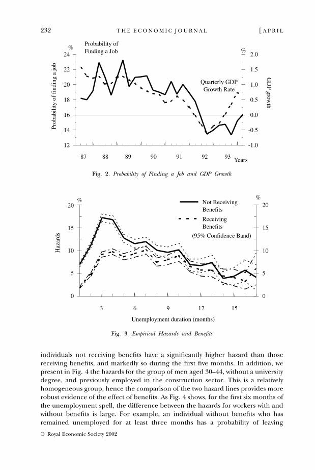
individuals not receiving benefits have a significantly higher hazard than thosereceiving benefits, and markedly so during the first five months. In addition, wepresent in Fig. 4 the hazards for the group of men aged 30–44, without a universitydegree, and previously employed in the construction sector. This is a relativelyhomogeneous group, hence the comparison of the two hazard lines provides morerobust evidence of the effect of benefits. As Fig. 4 shows, for the first six months ofthe unemployment spell, the difference between the hazards for workers with andwithout benefits is large. For example, an individual without benefits who hasremained unemployed for at least three months has a probability of leaving

Prob

abili

ty o

f fi

ndin

g a

job

24

22

20

18

16

14

12

87 88 89 90 91 92 93 Years

-1.0

-0.5

0.0

0.5

1.0

1.5

2.0

Probability ofFinding a Job

Quarterly GDPGrowth Rate

GD

P growth

%%

Fig. 2. Probability of Finding a Job and GDP Growth

Unemployment duration (months)

Haz

ards

3

0

5

10

15

20% %

6 9 12 15

0

5

10

15

20Not ReceivingBenefits

ReceivingBenefits

(95% Confidence Band)

Fig. 3. Empirical Hazards and Benefits



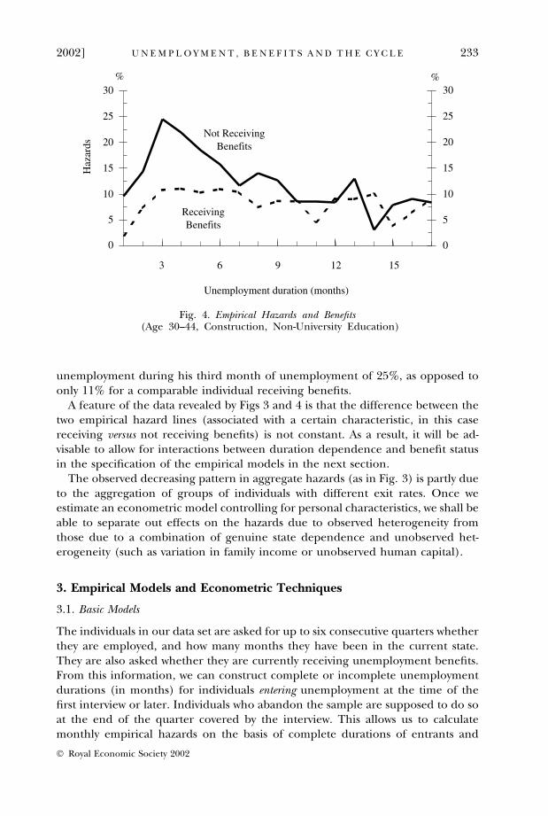
unemployment during his third month of unemployment of 25%, as opposed toonly 11% for a comparable individual receiving benefits.

A feature of the data revealed by Figs 3 and 4 is that the difference between thetwo empirical hazard lines (associated with a certain characteristic, in this casereceiving versus not receiving benefits) is not constant. As a result, it will be ad-visable to allow for interactions between duration dependence and benefit statusin the specification of the empirical models in the next section.

The observed decreasing pattern in aggregate hazards (as in Fig. 3) is partly dueto the aggregation of groups of individuals with different exit rates. Once weestimate an econometric model controlling for personal characteristics, we shall beable to separate out effects on the hazards due to observed heterogeneity fromthose due to a combination of genuine state dependence and unobserved het-erogeneity (such as variation in family income or unobserved human capital).

3. Empirical Models and Econometric Techniques

3.1. Basic Models

The individuals in our data set are asked for up to six consecutive quarters whetherthey are employed, and how many months they have been in the current state.They are also asked whether they are currently receiving unemployment benefits.From this information, we can construct complete or incomplete unemploymentdurations (in months) for individuals entering unemployment at the time of thefirst interview or later. Individuals who abandon the sample are supposed to do soat the end of the quarter covered by the interview. This allows us to calculatemonthly empirical hazards on the basis of complete durations of entrants and

Haz

ards

Not ReceivingBenefits

ReceivingBenefits


3

0

5

10

15

20

25

30

6 9 12 15

0

5

10

15

20

25

30%%

Fig. 4. Empirical Hazards and Benefits(Age 30–44, Construction, Non-University Education)



surviving non-censored samples for up to 17 months. We can also construct theduration of benefit entitlement for individuals whose unemployment durationexceeds their benefit duration. Otherwise, we only observe the event that benefitentitlement is at least as long as unemployment duration. In our analysis, we treatunemployment duration (T ) and benefit entitlement duration (B) as discreterandom variables that are subject to censoring. Unemployment duration is rightcensored when the individual is still unemployed at the time of leaving the sample.Benefit entitlement duration has a different type of censoring since its observa-bility depends on it being shorter than unemployment duration.

Let C be the number of periods the individual is in the sample after enteringunemployment. In our database, C is at least 2 quarters but not larger than 6quarters. We observe T if T < C; otherwise we only observe the event that T ‡ C.Moreover, we observe B if B < T < C. We assume that T and B are independent ofC, which is not an unreasonable assumption, given the rotating nature of ourpanel.

This observational plan motivates us to use, as the basis for our empirical analysisof the relationship between T and B, the hazard functions

/0ðtÞ ¼ PðT ¼ t j T � t;B < tÞ/1ðtÞ ¼ PðT ¼ t j T � t;B � tÞ

The function /0(t) gives the probability of being unemployed for exactly t monthsrelative to the group of individuals who have been unemployed for at least tmonths and do not receive benefits at t. On the other hand, /1(t) gives a similarprobability for individuals who are unemployed for t periods or more, but are stillreceiving benefits at t.

The comparison between /0(t) and /1(t) provides a basis for studying ameaningful effect of B on T because both probabilities are conditional on beingunemployed for t periods. In effect, regression or correlation analysis between Tand B would be difficult to interpret. The reason is that the limitation in time ofbenefit entitlement creates an association between being on benefits and observ-ing shorter unemployment durations which is unrelated to the effect of substantiveinterest.

To clarify the nature of our analysis, let us discuss how we would proceed if wecould observe benefit entitlement for all workers. If entitlement were not a cen-sored variable at B ‡ T, the following conditional hazard functions would beidentified for any entitlement s:

hðt; sÞ ¼ PðT ¼ t j T � t;B ¼ sÞ

In our dataset, h(t, s) is identified for s < t but not for s ‡ t. For example, withB ¼ 3, h(1, 3), h(2, 3), and h(3, 3) are not identified. So we cannot observe how thehazard rate for workers with benefits changes as the time of benefit exhaustionapproaches.

To examine the relationship between the benefit effects that we can identify andthe hazard rates conditional on benefit entitlement, notice that /0(t) and /1(t) arelinear combinations of h(t, s), such that we can write



/0ðtÞ � /1ðtÞ ¼Xt�1

s¼0

hðt; sÞwts �XS

s¼t

hðt; sÞw0ts

where S is the maximum value of B, and wts and w0ts are proper weights given by

wts ¼PðB ¼ s j T � tÞPðB < t j T � tÞ

and

w0ts ¼

PðB ¼ s j T � tÞPðB � t j T � tÞ

Suppose that h(t, s) ¼ /0(t) for s < t, but h(t, s) increases monotonically as tapproaches s for a given s ‡ t (i.e. the hazards for workers with and withoutbenefits begin to approach each other before benefit exhaustion, as the formerchange their behaviour in anticipation of the arrival of the exhaustion date). Insuch a case,

/0ðtÞ � /1ðtÞ ¼ RSs¼t ½/0ðtÞ � hðt; sÞw0

ts

can be regarded as a weighted average of the differences in hazards between thosewithout benefits and those with benefit entitlements greater than t. Thus, ourempirical difference will underestimate the difference in hazards for those whosebenefit exhaustion is sufficiently ahead of t, and overestimate it for the rest.Moreover, as t increases, the observed differences will be closer to the actualdifferences for the relevant levels of benefit entitlement.

A simple but restrictive specification under which knowledge of /0(t) and /1(t)suffices to determine h(t, s) is to assume that, at any t, there are only two possiblehazard rates depending on whether individuals receive benefits, for examplebecause there are only two search intensities. In other words:

hðt; sÞ ¼ /1ðtÞ for s � t/0ðtÞ for s < t

�

This two-regime hazard model is a restricted version of the standard model de-scribed in Section 1. The latter predicts that, for two individuals with benefits at agiven t, the one with shorter benefits has a greater hazard than the one with longerbenefits, whereas the former model assumes that the two are equal. This assump-tion is not testable, though, because we do not observe B for individuals with B ‡ T.

Given the two-regime model, it is possible to reconstruct the conditional dis-tributions of unemployment durations for a given level of benefit entitlement. Ineffect, we have

PðT > t j B ¼ sÞ ¼Yt

k¼1

½1 � hðk; sÞ t ¼ 1; 2; . . .

from which we can, for example, calculate the median unemployment duration fora given value of B, or changes in median duration from a change in benefitentitlement:

DðsÞ ¼ medðT j B ¼ s þ 1Þ � medðT j B ¼ sÞ



However, the distributions {T | B ¼ s} are not identified nonparametrically in ourdata, and they can only be identified owing to a functional form assumption likethe two-regime model. Therefore, we shall emphasise in our empirical analysis themodelling of /0(t) and /1(t), for which we have direct counterparts in the data. Atthe end of the paper, we shall, nevertheless, also present estimates of changes inmedian duration arising from changes in benefit entitlements.

A minor point is that, in our empirical analysis, we redefine /0(t) as

/0ðtÞ ¼ PðT ¼ t j T � t;B < t � 2Þ

to take into account that, while T is observed at monthly intervals, B is only ob-served at quarterly intervals (see Appendix 2). Obviously, this redefinition has noconsequences for the relation of /0(t) and /1(t) to the two-regime model.

In addition to benefits, our analysis is also conditional on age, education, headof household status, sector and year variables. Alternatively, year and sectoraldummies are replaced by aggregate and sectoral economic variables. The para-metric models that we consider are logistic hazards of the form

/ t; bðtÞ; xðtÞ½ � P T ¼ t j T � t; bðtÞ; xðtÞ½ ð1Þ¼ F ½h0ðtÞ þ h1ðtÞbðtÞ þ h2ðtÞxðtÞ þ h3ðtÞbðtÞxðtÞ;

where the new symbols are as follows. x(t) is the vector of conditioning individual,sectoral and aggregate variables, some of which are time-invariant like education,while others, like the aggregate economic variables, are time-varying. The variableb(t) is the binary indicator of whether the individual still has benefits in t:

bðtÞ ¼ 1ðB � tÞ:

F denotes the logistic cumulative distribution function: F(u) ¼ eu/(1 + eu). In ad-dition, h0(t) is an unrestricted parameter specific of each t that captures flexibleadditive duration dependence, and h1(t), h2(t) and h3(t) are polynomials in log twhose purpose is to capture interaction effects between duration and conditioningvariables.9

In our model, b(t) is a predetermined variable while the remaining time-varyingvariables in x(t) are strictly exogenous. This means that the probability in (1)should be understood as being conditional on the entire path of x(t) and thevalues of b(t) up to t, but not on b(t + 1), b(t + 2), etc. Namely, we assume

P T ¼ t j T � t; bð1Þ; . . . ; bðtÞ; xð1Þ; . . . ; xð1Þ½ ¼ P T ¼ t j T � t; bðtÞ; xðtÞ½ :

We treat b(t) as predetermined as opposed to strictly exogenous because, asexplained above, we would expect P[T ¼ t | T ‡ t, b(t), x(t)] to differ from theprobability conditional on benefit entitlement, which is equivalent to

P T ¼ t j T � t; bð1Þ; . . . ; bð1Þ; xð1Þ; . . . ; xð1Þ½ :

Note that b(t) would only be exogenous if the two-regime model were to hold.

9 Note that /[t, b(t), x(t)] is just a common notation for /0[t, x(t)] and /1[t, x(t)]: /[t, b(t),x(t)] ” [1 ) b(t)]/0[t, x(t)] + b(t)/1[t, x(t)], where we specify /0[t, x(t)] ¼ F [h0(t) + h2(t)x(t)], and/1[t, x(t)] ¼ F [h0(t) + h1(t) + h2(t)x(t) + h3(t)x(t)].



Whether b(t) is predetermined matters very little in the context of homogeneousmodels, but it will have the effect of rendering b(t) an endogenous variable whenwe consider models with unobserved heterogeneity.

A hazard function in which all the conditioning variables x(t) are strictly exo-genous corresponds to a conditional distribution of durations given the fullstochastic process for x(t). By contrast, in the predetermined case, we are effectivelyconsidering a sequence of hazard functions corresponding to different conditionaldistributions of durations. However, in the absence of unobserved heterogeneity,conditional inference is still possible, and we can rely on the same likelihoodestimation criterion under both assumptions. The interpretation of the criterion,however, differs in each case: while with strictly exogenous variables the criterionbelow is the actual conditional likelihood of the data, with predetermined variablesit can only be regarded as a partial likelihood; see Lancaster (1990, pp. 23–31) fora discussion of these issues.

A discrete duration model can be regarded as a sequence of binary choiceequations (with cross-equation restrictions) defined on the surviving population ateach duration. This provides a useful perspective, for both statistical and compu-tational reasons, that has been noted by a number of authors (Kiefer, 1987;Narendranathan and Stewart, 1993; Sueyoshi, 1995; Jenkins, 1995). It is also astraightforward way of motivating the estimation criterion for a duration modelwith predetermined variables.

To see this, let T 0i denote the observed censored duration variable, so that

T 0i ¼ Ti if Ti < Ci

Ci otherwise

�

and let ci denote the indicator of lack of censoring: ci ¼ 1(Ti < Ci). Moreover, let Yti

be a (0, 1) variable indicating whether the observed duration equals t: Yti ¼ 1ðT 0

i ¼ tÞ. Then the conditional log-likelihood of the sample for Yti given T 0i � t is

of the form

Lt ¼XN

i¼1

1ðT 0i � tÞ ciYti log /iðtÞ þ ð1 � ciYtiÞ log 1 � /iðtÞ½ f g

where N is the number of unemployment spells in the sample and

/iðtÞ ¼ / t; biðtÞ; xiðtÞ½

Combining the Lt for all observed durations, we obtain our estimating criterion:

LðhÞ ¼Xs

t¼1

Lt ð2Þ

¼XN

i¼1

ð1 � ciÞXT 0

i

t¼1

log½1 � /iðtÞ þ ci

XT 0i �1

t¼1

log 1 � /iðtÞ½ þ log /iðT 0i Þ

8<:

9=;

0@

1A

where h is the vector of parameters to be estimated and s is the largest observedduration.



We estimate h by maximising the partial likelihood L(h). Notice that L(h) is ofthe same form as a standard log-likelihood for censored discrete duration datawith strictly exogenous variables, although with a different interpretation whenconditioning on predetermined variables. In the absence of cross restrictionslinking the parameters h with those in the benefit indicator process, the partiallikelihood estimates of h will be asymptotically efficient.

3.2. Models with Unobserved Heterogeneity

The economic interpretation of the coefficients in model (1) is likely to behampered by unobserved heterogeneity. Aside from the problem of censoring inthe benefit entitlement variable discussed above, in our sample there are unob-served differences in family income and in the amount of benefits received.Moreover, individuals with and without benefits may differ in ways that we do notobserve. For example, there may be correlation between benefits and unobservedhuman capital variables.

Such unobserved heterogeneity is likely to bias downwards the effect of benefitson the exit rates, and to introduce spurious negative duration dependence. In theabsence of better data, it is unlikely that much more progress can be made onthese issues. However, it is still possible to generalise the standard specification bymaking the analysis conditional on an unobserved variable u with a known dis-tribution independent of the exogenous variables. Following the work of Heckmanand Singer (1984), the recent econometric literature has emphasised the casewhere u is a discrete random variable with finite support, thus giving rise to amixture model. This approach is attractive because it is flexible, and also because,by letting the support of u grow with sample size, it is possible to establish as-ymptotic properties for the estimators with respect to a model with an unspecifieddistribution for u.

Here we also follow this approach. In our case, the situation is fundamentallyaltered when unobserved heterogeneity is introduced, however, because we areconditioning on a predetermined variable. Unlike in the model with only strictlyexogenous variables, we cannot just consider a mixture version of (2), since (2) isin our case a partial likelihood. In fact, by introducing unobserved heterogeneity,b(t) becomes fully endogenous and we can no longer condition on it. We thereforeproceed by specifying a reduced form process for b(t) given u. In this way, we canallow for unobserved heterogeneity that is correlated with benefits but uncor-related with the exogenous variables. This procedure is analogous to that used byHam and LaLonde (1996), who specified a separate hazard and heterogeneityterm for initial conditions in their evaluation of the effect of training on em-ployment and unemployment spells; see also Meghir and Whitehouse (1997).A formalisation of these issues is presented in the following subsections.

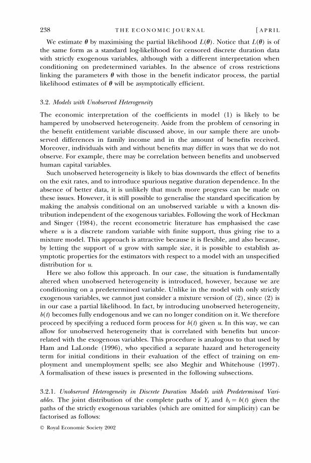
3.2.1. Unobserved Heterogeneity in Discrete Duration Models with Predetermined Vari-ables. The joint distribution of the complete paths of Yt and bt ¼ b(t) given thepaths of the strictly exogenous variables (which are omitted for simplicity) can befactorised as follows:



f ðY1; . . . ;Ys; b1; . . . ; bsÞ ¼ f1f2

where

f1 ¼ f1sðYs j Y s�1; bsÞ . . . f11ðY1 j b1Þf2 ¼ f2sðbs j Y s�1; bs�1Þ . . . f22ðb2 j Y1; b1Þf21ðb1Þ

and we use the notation Y t ¼ (Y1, …, Yt) and bt ¼ (b1, …, bt).Under strict exogeneity, that is, given Granger non-causality,

f2 ¼ f ðb1; . . . ; bsÞ

and f1 becomes the conditional likelihood of Y s given bs. Otherwise, it is just apartial likelihood. But, in either case, we can conduct inferences on the parame-ters in f1 disregarding f2, provided those parameters are identified in f1 alone.

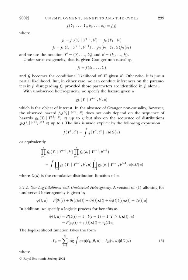
With unobserved heterogeneity, we specify the hazard given u

g1tðYt j Y t�1; bt ;uÞ

which is the object of interest. In the absence of Granger non-causality, however,the observed hazard f1t(Yt | Y t-1, bt) does not only depend on the sequence ofhazards g1s(Ys | Y s-1, bs, u) up to t, but also on the sequence of distributionsg2s(bs | Y s-1, bs-1,u) up to t. The link is made explicit by the following expression

f ðY s; bsÞ ¼Z

g ðY s; bs j uÞdGðuÞ

or equivalentlyYs

t¼1

f1tðYt j Y t�1; btÞYs

t¼1

f2tðbt j Y t�1; bt�1Þ

¼Z Ys

t¼1

g1tðYt j Y t�1; bt ;uÞYs

t¼1

g2tðbt j Y t�1; bt�1;uÞdGðuÞ

where G(u) is the cumulative distribution function of u.

3.2.2. Our Log-Likelihood with Unobserved Heterogeneity. A version of (1) allowing forunobserved heterogeneity is given by

/ðt;uÞ ¼ F ½h0ðtÞ þ h1ðtÞbðtÞ þ h2ðtÞxðtÞ þ h3ðtÞbðtÞxðtÞ þ h4ðtÞu

In addition, we specify a logistic process for benefits as

wðt;uÞ ¼ PðbðtÞ ¼ 1 j bðt � 1Þ ¼ 1;T � t; xðtÞ;uÞ¼ F c0ðtÞ þ c1ðtÞxðtÞ þ c2ðtÞu½

The log-likelihood function takes the form

Lh ¼XN

i¼1

log

Zexp½‘1iðh;uÞ þ ‘2iðc;uÞdGðuÞ ð3Þ

where



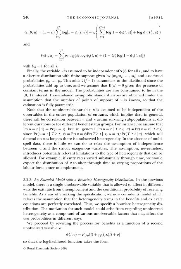
‘1iðh;uÞ ¼ ð1 � ciÞXT 0

i

t¼1

log 1 � /iðt;uÞ½ þ ci

XT 0i �1

t¼1

log 1 � /iðt;uÞ½ þ log /iðT 0i ;uÞ

8<:

9=;

and

‘2iðc;uÞ ¼XT 0

i

t¼1

biðt�1Þ bit log wiðt;uÞ þ ð1 � bitÞ log 1 � wiðt;uÞ½ f g

with bi0 ¼ 1 for all i.Finally, the variable u is assumed to be independent of x(t) for all t , and to have

a discrete distribution with finite support given by {m1,m2, …, mj } and associatedprobabilities p1, …, pj . This adds 2(j ) 1) parameters to the likelihood since theprobabilities add up to one, and we assume that E(u) ¼ 0 given the presence ofconstant terms in the model. The probabilities are also constrained to lie in the(0, 1) interval. Hessian-based asymptotic standard errors are obtained under theassumption that the number of points of support of u is known, so that theestimation is fully parametric.

Note that the unobservable variable u is assumed to be independent of theobservables in the entire population of entrants, which implies that, in general,there will be correlation between u and x within surviving subpopulations at dif-ferent durations or for different benefit status groups. For instance, we assume thatPr(u ¼ r | x) ¼ Pr(u ¼ r) but in general Pr(u ¼ r | T ‡ t, x) „ Pr(u ¼ r | T ‡ t)since Pr(u ¼ r | T ‡ t, x) ¼ Pr(u ¼ r)Pr(T ‡ t | x, u ¼ r)/Pr(T ‡ t | x), which willdepend on x as long as there is unobserved heterogeneity. In the absence of multi-spell data, there is little we can do to relax the assumption of independencebetween u and the strictly exogenous variables. The assumption, nevertheless,introduces potentially relevant limitations to the type of heterogeneity that can beallowed. For example, if entry rates varied substantially through time, we wouldexpect the distribution of u to alter through time as varying proportions of thelabour force enter unemployment.

3.2.3. An Extended Model with a Bivariate Heterogeneity Distribution. In the previousmodel, there is a single unobservable variable that is allowed to affect in differentways the exit rate from unemployment and the conditional probability of receivingbenefits. As a way of checking the specification, we now consider a model whichrelaxes the assumption that the heterogeneity terms in the benefits and exit rateequations are perfectly correlated. Thus, we specify a bivariate heterogeneity dis-tribution. The motivation for such model could arise from regarding unobservedheterogeneity as a compound of various unobservable factors that may affect thetwo probabilities in different ways.

We proceed by rewriting the process for benefits as a function of a secondunobserved variable v:

wðt; vÞ ¼ F c0ðtÞ þ c1ðtÞxðtÞ þ v½

so that the log-likelihood function takes the form



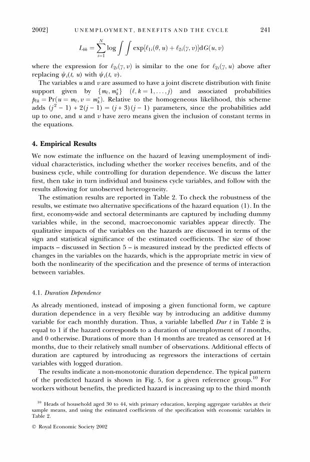
Lbh ¼XN

i¼1

log

Z Zexp½‘1iðh;uÞ þ ‘2iðc; vÞdGðu; vÞ

where the expression for ‘2iðc; vÞ is similar to the one for ‘2iðc;uÞ above afterreplacing wi(t, u) with wi(t, v).

The variables u and v are assumed to have a joint discrete distribution with finitesupport given by fm‘;m�

kg ð‘; k ¼ 1; . . . ; jÞ and associated probabilitiesp‘k ¼ Prðu ¼ m‘; v ¼ m�

k Þ. Relative to the homogeneous likelihood, this schemeadds (j 2 ) 1) + 2(j ) 1) ¼ (j + 3)(j ) 1) parameters, since the probabilities addup to one, and u and v have zero means given the inclusion of constant terms inthe equations.

4. Empirical Results

We now estimate the influence on the hazard of leaving unemployment of indi-vidual characteristics, including whether the worker receives benefits, and of thebusiness cycle, while controlling for duration dependence. We discuss the latterfirst, then take in turn individual and business cycle variables, and follow with theresults allowing for unobserved heterogeneity.

The estimation results are reported in Table 2. To check the robustness of theresults, we estimate two alternative specifications of the hazard equation (1). In thefirst, economy-wide and sectoral determinants are captured by including dummyvariables while, in the second, macroeconomic variables appear directly. Thequalitative impacts of the variables on the hazards are discussed in terms of thesign and statistical significance of the estimated coefficients. The size of thoseimpacts – discussed in Section 5 – is measured instead by the predicted effects ofchanges in the variables on the hazards, which is the appropriate metric in view ofboth the nonlinearity of the specification and the presence of terms of interactionbetween variables.

4.1. Duration Dependence

As already mentioned, instead of imposing a given functional form, we captureduration dependence in a very flexible way by introducing an additive dummyvariable for each monthly duration. Thus, a variable labelled Dur t in Table 2 isequal to 1 if the hazard corresponds to a duration of unemployment of t months,and 0 otherwise. Durations of more than 14 months are treated as censored at 14months, due to their relatively small number of observations. Additional effects ofduration are captured by introducing as regressors the interactions of certainvariables with logged duration.

The results indicate a non-monotonic duration dependence. The typical patternof the predicted hazard is shown in Fig. 5, for a given reference group.10 Forworkers without benefits, the predicted hazard is increasing up to the third month

10 Heads of household aged 30 to 44, with primary education, keeping aggregate variables at theirsample means, and using the estimated coefficients of the specification with economic variables inTable 2.



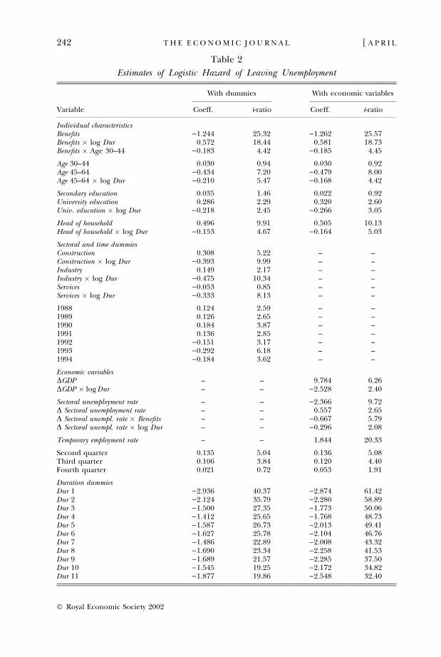
Table 2

Estimates of Logistic Hazard of Leaving Unemployment

With dummies With economic variables

Variable Coeff. t-ratio Coeff. t-ratio

Individual characteristicsBenefits )1.244 25.32 )1.262 25.57Benefits � log Dur 0.572 18.44 0.581 18.73Benefits � Age 30–44 )0.183 4.42 )0.185 4.45

Age 30–44 0.030 0.94 0.030 0.92Age 45–64 )0.434 7.20 )0.479 8.00Age 45–64 � log Dur )0.210 5.47 )0.168 4.42

Secondary education 0.035 1.46 0.022 0.92University education 0.286 2.29 0.320 2.60Univ. education � log Dur )0.218 2.45 )0.266 3.05

Head of household 0.496 9.91 0.505 10.13Head of household � log Dur )0.153 4.67 )0.164 5.03

Sectoral and time dummiesConstruction 0.308 5.22 – –Construction � log Dur )0.393 9.99 – –Industry 0.149 2.17 – –Industry � log Dur )0.475 10.34 – –Services )0.053 0.85 – –Services � log Dur )0.333 8.13 – –

1988 0.124 2.59 – –1989 0.126 2.65 – –1990 0.184 3.87 – –1991 0.136 2.85 – –1992 )0.151 3.17 – –1993 )0.292 6.18 – –1994 )0.184 3.62 – –

Economic variablesDGDP – – 9.784 6.26DGDP � log Dur – – )2.528 2.40

Sectoral unemployment rate – – )2.366 9.72D Sectoral unemployment rate – – 0.557 2.65D Sectoral unempl. rate � Benefits – – )0.667 5.79D Sectoral unempl. rate � log Dur – – )0.296 2.08

Temporary employment rate – – 1.844 20.33

Second quarter 0.135 5.04 0.136 5.08Third quarter 0.106 3.84 0.120 4.40Fourth quarter 0.021 0.72 0.053 1.91

Duration dummiesDur 1 )2.936 40.37 )2.874 61.42Dur 2 )2.124 35.79 )2.280 58.89Dur 3 )1.500 27.35 )1.773 50.06Dur 4 )1.412 25.65 )1.768 48.73Dur 5 )1.587 26.73 )2.013 49.41Dur 6 )1.627 25.78 )2.104 46.76Dur 7 )1.486 22.89 )2.008 43.32Dur 8 )1.690 23.34 )2.258 41.53Dur 9 )1.689 21.57 )2.285 37.50Dur 10 )1.545 19.25 )2.172 34.82Dur 11 )1.877 19.86 )2.548 32.40



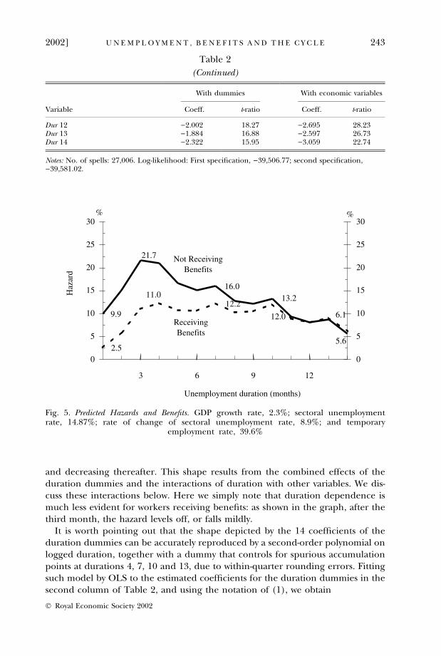
and decreasing thereafter. This shape results from the combined effects of theduration dummies and the interactions of duration with other variables. We dis-cuss these interactions below. Here we simply note that duration dependence ismuch less evident for workers receiving benefits: as shown in the graph, after thethird month, the hazard levels off, or falls mildly.

It is worth pointing out that the shape depicted by the 14 coefficients of theduration dummies can be accurately reproduced by a second-order polynomial onlogged duration, together with a dummy that controls for spurious accumulationpoints at durations 4, 7, 10 and 13, due to within-quarter rounding errors. Fittingsuch model by OLS to the estimated coefficients for the duration dummies in thesecond column of Table 2, and using the notation of (1), we obtain

Table 2

(Continued)

With dummies With economic variables


Dur 12 )2.002 18.27 )2.695 28.23Dur 13 )1.884 16.88 )2.597 26.73Dur 14 )2.322 15.95 )3.059 22.74

Notes: No. of spells: 27,006. Log-likelihood: First specification, )39,506.77; second specification,)39,581.02.

Not ReceivingBenefits

ReceivingBenefits


3

2.5

9.9

11.0

21.7

16.013.2

12.2

12.0 6.1

5.6

0

5

10

15

20

25

30

0

5

10

15

20

25

30% %

6 9 12

Haz

ard

Fig. 5. Predicted Hazards and Benefits. GDP growth rate, 2.3%; sectoral unemploymentrate, 14.87%; rate of change of sectoral unemployment rate, 8.9%; and temporary

employment rate, 39.6%



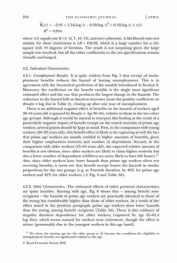
bhh0ðtÞ ¼ �2:91 þ 1:54ðlog tÞ � 0:59ðlog tÞ2 þ 0:10ðlog tÞ � r ðtÞR2 ¼ 0:954

where r(t) equals one if t ˛ {4, 7, 10, 13}, and zero otherwise. A likelihood ratio teststatistic for these restrictions is LR ¼ 102.62, which is a large number for a chi-square with 10 degrees of freedom. The result is not surprising given the largesample size involved, but all the other coefficients in the two specifications remainvirtually unchanged.

4.2. Individual Characteristics

4.2.1. Unemployment Benefits. It is quite evident from Fig. 5 that receipt of unem-ployment benefits reduces the hazard of leaving unemployment. This is inagreement with the theoretical prediction of the models introduced in Section 2.Moreover, the coefficient on the benefit variable is the single most significantestimated effect and the one that produces the largest change in the hazards. Thereduction in the hazard falls as duration increases (note the positive coefficient onBenefits · log Dur in Table 2), closing up after one year of unemployment.

There is an additional negative effect of benefits on the hazards of workers aged30–44 years old (captured by Benefits · Age 30–44), relative to those in the two otherage groups. Although it would be natural to interpret this finding as the result of aparticularly negative impact of benefit receipt on the search intensity of prime ageworkers, several points should be kept in mind. First, in the comparison with youngworkers (20–29 years old), this benefit effect is likely to be capturing as well the factthat prime age workers are usually entitled to higher amounts of benefits, giventheir higher employment seniority and number of dependants. Second, in thecomparison with older workers (45–64 years old), the expected relative amount ofbenefits is not obvious, since older workers are likely to claim higher seniority butalso a lower number of dependants (children are more likely to have left home).11

Also, since older workers have lower hazards than prime age workers when notreceiving benefits, it turns out that benefit receipt lowers the hazards in similarproportions for the two groups (e.g. at 3-month duration, by 49% for prime ageworkers and 42% for older workers, c.f. Fig. 6 and Table A6).

4.2.2. Other Characteristics. The estimated effects of other personal characteristicsare quite intuitive. Starting with age, Fig. 6 shows that – among benefit non-recipients – the hazards of prime age workers are practically identical to those ofthe young but considerably higher than those of older workers. As a result of theeffect noted in the previous paragraph, prime age workers show lower hazardsthan the young, among benefit recipients (Table A6). There is also evidence ofnegative duration dependence for older workers (captured by Age 45–64 ·log Dur), which seems natural for workers near retirement, though the effect isminor (presumably due to the youngest workers in this age band).

11 We chose the starting age for the older group at 45 because the conditions for eligibility tounemployment benefits are significantly relaxed at this age.



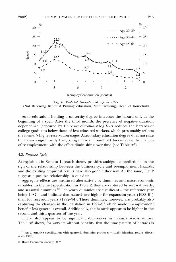
As to education, holding a university degree increases the hazard only at thebeginning of a spell. After the third month, the presence of negative durationdependence (captured by University education · log Dur) reduces the hazards ofcollege graduates below those of less educated workers, which presumably reflectsthe former’s higher reservation wages. A secondary education degree does not raisethe hazards significantly. Last, being a head of household does increase the chancesof re-employment, with the effect diminishing over time (see Table A6).

4.3. Business Cycle

As explained in Section 1, search theory provides ambiguous predictions on thesign of the relationship between the business cycle and re-employment hazards,and the existing empirical results have also gone either way. All the same, Fig. 2suggests a positive relationship in our data.

Aggregate effects are measured alternatively by dummies and macroeconomicvariables. In the first specification in Table 2, they are captured by sectoral, yearly,and seasonal dummies.12 The yearly dummies are significant – the reference yearbeing 1987 – and indicate that hazards are higher for expansion years (1988–91)than for recession years (1992–94). These dummies, however, are probably alsocapturing the changes in the legislation in 1992–93 which made unemploymentbenefits less generous overall. Additionally, the hazards appear to be higher in thesecond and third quarters of the year.

There also appear to be significant differences in hazards across sectors.Table A6 shows, for workers without benefits, that the time pattern of hazards is

22.3

21.8

11.9

11.612.5

7.96.7

14.2

14.6

11.4

11.1

4.84.6

4.4

1.7

3

0

5

10

15

20

25

30

0

5

10

15

20

25

30Age 20–29

Age 30–44

Age 45–64

%%

6 9 12

Haz

ard


Fig. 6. Predicted Hazards and Age in 1989(Not Receiving Benefits) Primary education, Manufacturing, Head of household

12 An alternative specification with quarterly dummies produces virtually identical results (Boveret al., 1996).



similar across sectors – slightly flatter in agriculture, but the levels are quite dif-ferent. The ordering of sectors in terms of the hazard of finding a job, from highestto lowest, is: agriculture, construction, services and manufacturing. This order doesnot match the ranking of the sectoral unemployment rates in Spain well, which overthe sample period was: services (10.4%), manufacturing (11.5%), agriculture(13.4%) and construction (20.4%). In particular, the two sectors with the lowestunemployment rates show the lowest hazards of leaving unemployment, and viceversa. The puzzle is resolved once we realise that we are only analysing unemploy-ment outflows and ignoring inflows. The outflow ordering we have obtained is, onthe other hand, correlated with the sectoral ranking in terms of the proportion oftemporary employment, as described in Section 2. Thus we shall include temporaryemployment rates by sector as explanatory variables below.

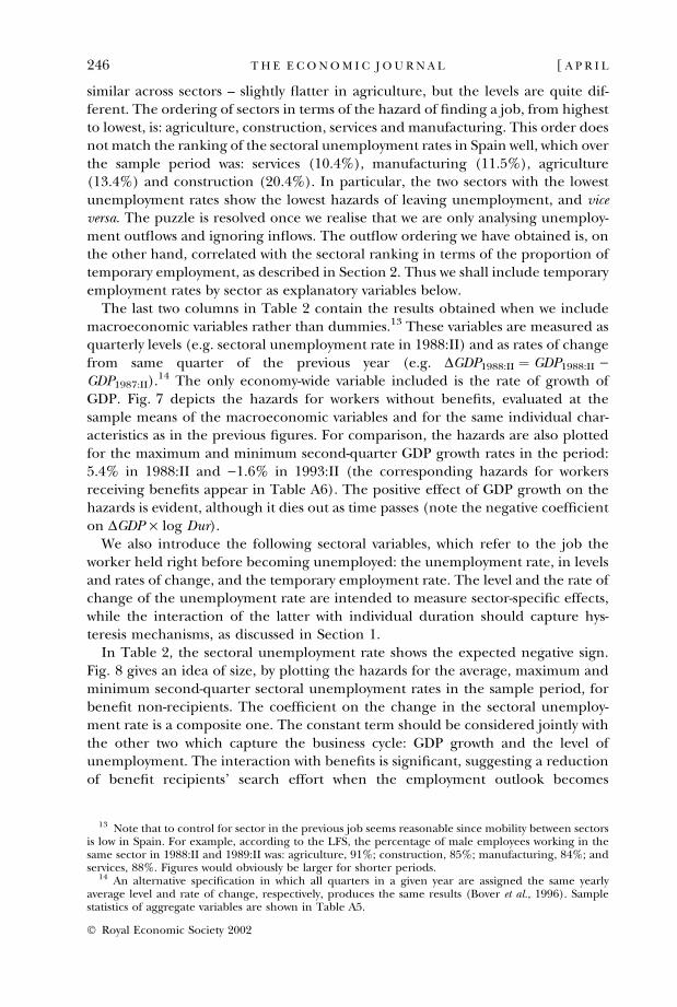
The last two columns in Table 2 contain the results obtained when we includemacroeconomic variables rather than dummies.13 These variables are measured asquarterly levels (e.g. sectoral unemployment rate in 1988:II) and as rates of changefrom same quarter of the previous year (e.g. DGDP1988:II ¼ GDP1988:II )GDP1987:II).14 The only economy-wide variable included is the rate of growth ofGDP. Fig. 7 depicts the hazards for workers without benefits, evaluated at thesample means of the macroeconomic variables and for the same individual char-acteristics as in the previous figures. For comparison, the hazards are also plottedfor the maximum and minimum second-quarter GDP growth rates in the period:5.4% in 1988:II and )1.6% in 1993:II (the corresponding hazards for workersreceiving benefits appear in Table A6). The positive effect of GDP growth on thehazards is evident, although it dies out as time passes (note the negative coefficienton DGDP · log Dur).

We also introduce the following sectoral variables, which refer to the job theworker held right before becoming unemployed: the unemployment rate, in levelsand rates of change, and the temporary employment rate. The level and the rate ofchange of the unemployment rate are intended to measure sector-specific effects,while the interaction of the latter with individual duration should capture hys-teresis mechanisms, as discussed in Section 1.

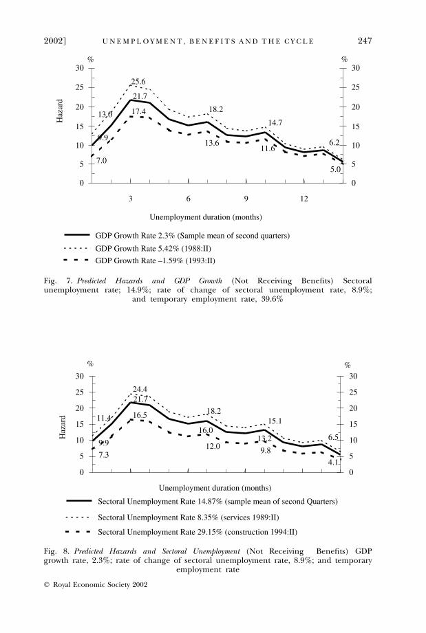
In Table 2, the sectoral unemployment rate shows the expected negative sign.Fig. 8 gives an idea of size, by plotting the hazards for the average, maximum andminimum second-quarter sectoral unemployment rates in the sample period, forbenefit non-recipients. The coefficient on the change in the sectoral unemploy-ment rate is a composite one. The constant term should be considered jointly withthe other two which capture the business cycle: GDP growth and the level ofunemployment. The interaction with benefits is significant, suggesting a reductionof benefit recipients’ search effort when the employment outlook becomes

13 Note that to control for sector in the previous job seems reasonable since mobility between sectorsis low in Spain. For example, according to the LFS, the percentage of male employees working in thesame sector in 1988:II and 1989:II was: agriculture, 91%; construction, 85%; manufacturing, 84%; andservices, 88%. Figures would obviously be larger for shorter periods.

14 An alternative specification in which all quarters in a given year are assigned the same yearlyaverage level and rate of change, respectively, produces the same results (Bover et al., 1996). Samplestatistics of aggregate variables are shown in Table A5.



%30

25

20

15

10

5

0

30

25

20

15

10

5

0


24.421.7

16.511.4

9.9

7.312.0

16.0

18.215.1

13.2

9.8

6.5

4.1

%

Haz

ard

Sectoral Unemployment Rate 14.87% (sample mean of second Quarters)

Sectoral Unemployment Rate 8.35% (services 1989:II)

Sectoral Unemployment Rate 29.15% (construction 1994:II)

Fig. 8. Predicted Hazards and Sectoral Unemployment (Not Receiving Benefits) GDPgrowth rate, 2.3%; rate of change of sectoral unemployment rate, 8.9%; and temporary

employment rate

Haz

ard

% %

25.6

21.7

13.0

9.9

7.0

17.4 18.2

13.611.6

14.7

6.2

5.0

12963

0

5

10

15

20

25

30

0

5

10

GDP Growth Rate 2.3% (Sample mean of second quarters)

GDP Growth Rate 5.42% (1988:II)

GDP Growth Rate –1.59% (1993:II)

15

20

25

30


Fig. 7. Predicted Hazards and GDP Growth (Not Receiving Benefits) Sectoralunemployment rate; 14.9%; rate of change of sectoral unemployment rate, 8.9%;

and temporary employment rate, 39.6%



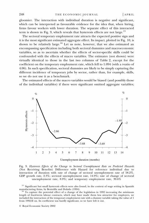
gloomier. The interaction with individual duration is negative and significant,which can be interpreted as favourable evidence for the idea that, when hiring,firms favour workers with lower duration. The separate effect of this interactedterm is shown in Fig. 9, which reveals that hysteresis effects are not large.15

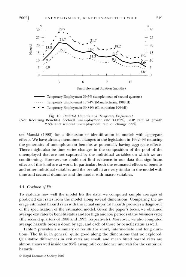
The sectoral temporary employment rate attracts the expected positive sign andit is the most significant estimated aggregate effect. Its impact, plotted in Fig. 10, isshown to be relatively large.16 Let us note, however, that we also estimated anencompassing specification including both sectoral dummies and macroeconomicvariables, so as to ascertain whether the effects of sector-specific skills could beconfounded with the effects of macro variables. The estimates (not shown) werevirtually identical to those in the last two columns of Table 2, except for thecoefficient on the temporary employment rate, which fell to 1.094 (with a t-ratio of4.06). In such specification, sectoral dummies are likely to be simply capturing thedifferent incidence of temporary jobs by sector, rather than, for example, skills,so we do not use it as a benchmark.

The estimated effects of the macro variables would be biased (and possibly thoseof the individual variables) if there were significant omitted aggregate variables;

Hys

tere

sis

effe

cts


1 2 3 4 5 6 7

–2.66

–3.68 –3.69

–1.95

8 9 10 11 12 13 14

–4

–3

–2

–1

0

–4

–3

–2

–1

0

%%

Fig. 9. Hysteresis Effects of the Change in Sectoral Unemployment Rate on Predicted Hazards(Not Receiving Benefits) Difference with Hazard for reference individual due tointeraction of duration with rate of change of sectoral unemployment rate of 58.2%.GDP growth rate, 2.3%; sectoral unemployment rate, 14.9%; rate of change of sectoral

unemployment rate, 8.9%; and temporary employment rate, 39.6%

15 Significant but small hysteresis effects were also found, in the context of wage setting in Spanishmanufacturing firms, by Bentolila and Dolado (1994).

16 To capture the potential effect of a change of the legislation in 1992 increasing the minimumlength of fixed-term labour contracts, which may have made them less attractive for employers, weincluded the interaction of the temporary employment rate with a dummy variable taking the value of 1from 1992:II on. Its coefficient was hardly significant, so we have left it out.



see Manski (1993) for a discussion of identification in models with aggregateeffects. We have already mentioned changes in the legislation in 1992–93 reducingthe generosity of unemployment benefits as potentially having aggregate effects.There might also be time series changes in the composition of the pool of theunemployed that are not captured by the individual variables on which we areconditioning. However, we could not find evidence in our data that significanteffects of this kind are at work. In particular, both the estimated effects of benefitsand other individual variables and the overall fit are very similar in the model withtime and sectoral dummies and the model with macro variables.

4.4. Goodness of Fit

To evaluate how well the model fits the data, we computed sample averages ofpredicted exit rates from the model along several dimensions. Comparing the av-erage estimated hazard rates with the actual empirical hazards provides a diagnosticof the specification of the estimated model. Given the paper’s focus, we obtainedaverage exit rates by benefit status and for high and low periods of the business cycle(the second quarters of 1988 and 1993, respectively). Moreover, we also computedaverage hazards broken down by age, and each of those by benefit status as well.

Table 3 provides a summary of results for short, intermediate and long dura-tions. The fit is, in general, quite good along the dimensions that we explored.Qualitative differences in exit rates are small, and mean fitted hazard rates arealmost always well inside the 95% asymptotic confidence intervals for the empiricalhazards.

Haz

ard


3

6.9

9.9

13.8

28.7

21.7

15.7

21.7

16.0

11.3

18.2

13.2

9.38.0

5.6

3.8

30

25

% %

20

15

10

5

0

30

25

20

15

10

5

0

Temporary Employment 39.6% (sample mean of second quarters)

Temporary Employment 17.94% (Manufacturing 1988:II)

Temporary Employment 59.84% (Construction 1994:II)

6 9 12

Fig. 10. Predicted Hazards and Temporary Employment(Not Receiving Benefits) Sectoral unemployment rate 14.87%, GDP rate of growth

2.3% and sectoral unemployment rate of change 8.9%



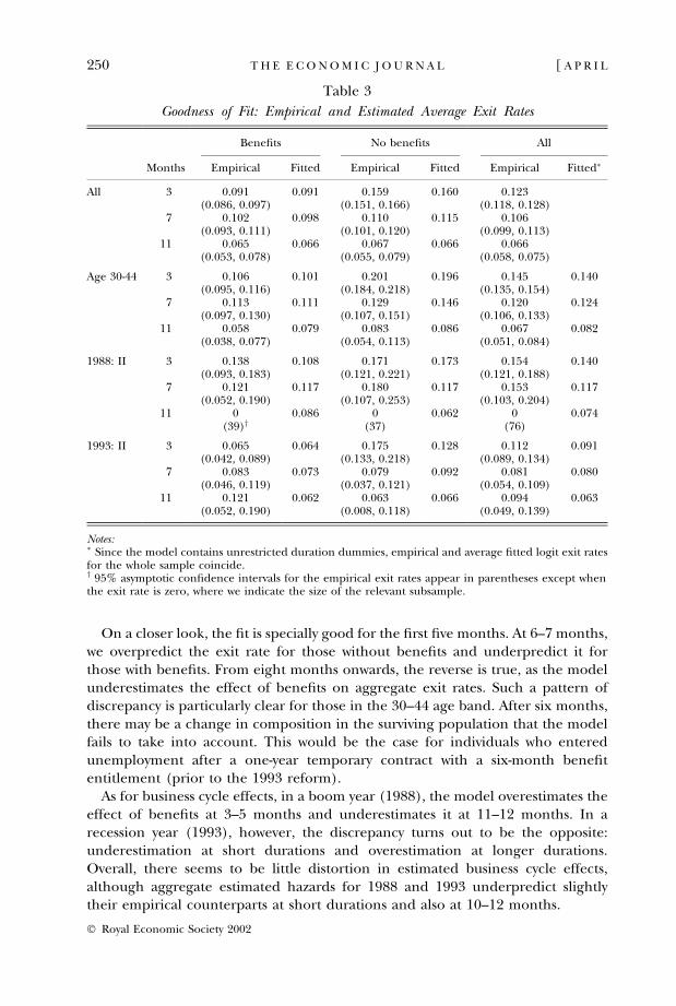
On a closer look, the fit is specially good for the first five months. At 6–7 months,we overpredict the exit rate for those without benefits and underpredict it forthose with benefits. From eight months onwards, the reverse is true, as the modelunderestimates the effect of benefits on aggregate exit rates. Such a pattern ofdiscrepancy is particularly clear for those in the 30–44 age band. After six months,there may be a change in composition in the surviving population that the modelfails to take into account. This would be the case for individuals who enteredunemployment after a one-year temporary contract with a six-month benefitentitlement (prior to the 1993 reform).

As for business cycle effects, in a boom year (1988), the model overestimates theeffect of benefits at 3–5 months and underestimates it at 11–12 months. In arecession year (1993), however, the discrepancy turns out to be the opposite:underestimation at short durations and overestimation at longer durations.Overall, there seems to be little distortion in estimated business cycle effects,although aggregate estimated hazards for 1988 and 1993 underpredict slightlytheir empirical counterparts at short durations and also at 10–12 months.

Table 3

Goodness of Fit: Empirical and Estimated Average Exit Rates

Benefits No benefits All

Months Empirical Fitted Empirical Fitted Empirical Fitted�

All 3 0.091 0.091 0.159 0.160 0.123(0.086, 0.097) (0.151, 0.166) (0.118, 0.128)

7 0.102 0.098 0.110 0.115 0.106(0.093, 0.111) (0.101, 0.120) (0.099, 0.113)

11 0.065 0.066 0.067 0.066 0.066(0.053, 0.078) (0.055, 0.079) (0.058, 0.075)

Age 30-44 3 0.106 0.101 0.201 0.196 0.145 0.140(0.095, 0.116) (0.184, 0.218) (0.135, 0.154)

7 0.113 0.111 0.129 0.146 0.120 0.124(0.097, 0.130) (0.107, 0.151) (0.106, 0.133)

11 0.058 0.079 0.083 0.086 0.067 0.082(0.038, 0.077) (0.054, 0.113) (0.051, 0.084)

1988: II 3 0.138 0.108 0.171 0.173 0.154 0.140(0.093, 0.183) (0.121, 0.221) (0.121, 0.188)

7 0.121 0.117 0.180 0.117 0.153 0.117(0.052, 0.190) (0.107, 0.253) (0.103, 0.204)

11 0 0.086 0 0.062 0 0.074(39)y (37) (76)

1993: II 3 0.065 0.064 0.175 0.128 0.112 0.091(0.042, 0.089) (0.133, 0.218) (0.089, 0.134)

7 0.083 0.073 0.079 0.092 0.081 0.080(0.046, 0.119) (0.037, 0.121) (0.054, 0.109)

11 0.121 0.062 0.063 0.066 0.094 0.063(0.052, 0.190) (0.008, 0.118) (0.049, 0.139)

Notes:� Since the model contains unrestricted duration dummies, empirical and average fitted logit exit ratesfor the whole sample coincide.y 95% asymptotic confidence intervals for the empirical exit rates appear in parentheses except whenthe exit rate is zero, where we indicate the size of the relevant subsample.



4.5. Unobserved Heterogeneity

We now turn to the estimation of the model for the hazard of leaving unemploymentwith unobserved heterogeneity presented in Section 3.2, which entails endogenisingbenefit receipt. Estimates of the joint mixture log-likelihood for unemploymentduration and benefit receipt, as specified in (3), are contained in Table 4. We do notallow any interaction of the effect of the unobserved variable u with duration. Thus,in terms of the notation of Section 3.2.2, the coefficients associated with u in theunemployment and benefits hazards are, respectively, h4(t) ¼ 1 and c2(t) ¼ c2.Moreover, we specify a distribution for u with two mass points, m1 and m2, withprobabilities p1 and p2. However, since E(u) ¼ 0, we are effectively introducing threeadditional free parameters in the model: m1, p1, and c2, which, together with the 35parameters in the unemployment hazard and the 32 parameters in the benefitsprocess, gives a total of 70 parameters in the mixture log-likelihood.

We need not devote much effort to interpreting the estimates on benefit receipt,since this is just an auxiliary reduced-form equation. Notice that we are concerned,for the first month of unemployment, with the probability that the worker isentitled to benefits on becoming unemployed while, in subsequent periods, wehave the probability that the worker is entitled to benefits given that he has re-mained unemployed until the current month and was entitled to benefits in theprevious month. The first probability depends on eligibility rules and the re-maining ones on benefit duration rules. Both types of rules, however, depend onthe type of benefits received. Eligibility to unemployment insurance depends onlyon tenure in the previous job while, for unemployment assistance, it depends onthe number of dependants, family income and age. Some regressors are cor-related with both rules in the same way. For example, the worker’s age or being ahead of household should be positively correlated with eligibility to both UI andUA. But, for other variables, the signs may differ. For example, the correlationbetween higher education and eligibility should be positive for UI (through longeremployment tenure) but negative for UA (through higher family income).

The last two columns in Table 4 show the results for a very general specificationincluding interactions of the regressors with unemployment duration (retainingonly the significant coefficients).17 We include as a regressor a step dummy startingin April 1992, to capture the legal change raising the stringency of UI eligibility.18

The results are quite intuitive and we do indeed find, in two instances, differencesbetween the results for the first month and thereafter. According to our estimates,the conditional probability of receiving benefits:

(a) increases with age (after the first month for workers aged 45–64), universityeducation (after the second month), and head of household status,

(b) falls with the sectoral proportion of temporary employment,

17 The results from estimating the reduced form process for the benefit receipt indicator separatelyare very close to the ones shown in Table 4 (Bover et al., 1996).

18 A dummy starting in April 1989 interacted with Age 45–64, meant to capture an extension of UAeligibility for that group of workers, was not significant. This was expected, since the change mostlyaffected workers after having received UA benefits for at least 18 months, a duration which is absent inour data. Legislative changes in 1993 affected benefit amounts but not eligibility rules.



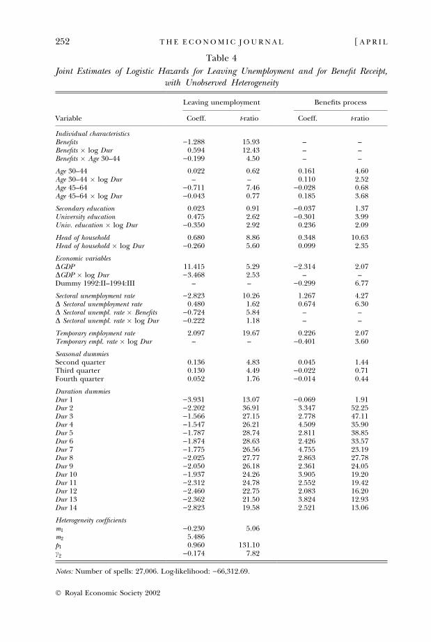
Table 4

Joint Estimates of Logistic Hazards for Leaving Unemployment and for Benefit Receipt,with Unobserved Heterogeneity

Leaving unemployment Benefits process


Individual characteristicsBenefits )1.288 15.93 – –Benefits � log Dur 0.594 12.43 – –Benefits � Age 30–44 )0.199 4.50 – –

Age 30–44 0.022 0.62 0.161 4.60Age 30–44 � log Dur – – 0.110 2.52Age 45–64 )0.711 7.46 )0.028 0.68Age 45–64 � log Dur )0.043 0.77 0.185 3.68

Secondary education 0.023 0.91 )0.037 1.37University education 0.475 2.62 )0.301 3.99Univ. education � log Dur )0.350 2.92 0.236 2.09

Head of household 0.680 8.86 0.348 10.63Head of household � log Dur )0.260 5.60 0.099 2.35

Economic variablesDGDP 11.415 5.29 )2.314 2.07DGDP � log Dur )3.468 2.53 – –Dummy 1992:II–1994:III – – )0.299 6.77

Sectoral unemployment rate )2.823 10.26 1.267 4.27D Sectoral unemployment rate 0.480 1.62 0.674 6.30D Sectoral unempl. rate � Benefits )0.724 5.84 – –D Sectoral unempl. rate � log Dur )0.222 1.18 – –

Temporary employment rate 2.097 19.67 0.226 2.07Temporary empl. rate � log Dur – – )0.401 3.60

Seasonal dummiesSecond quarter 0.136 4.83 0.045 1.44Third quarter 0.130 4.49 )0.022 0.71Fourth quarter 0.052 1.76 )0.014 0.44

Duration dummiesDur 1 )3.931 13.07 )0.069 1.91Dur 2 )2.202 36.91 3.347 52.25Dur 3 )1.566 27.15 2.778 47.11Dur 4 )1.547 26.21 4.509 35.90Dur 5 )1.787 28.74 2.811 38.85Dur 6 )1.874 28.63 2.426 33.57Dur 7 )1.775 26.56 4.755 23.19Dur 8 )2.025 27.77 2.863 27.78Dur 9 )2.050 26.18 2.361 24.05Dur 10 )1.937 24.26 3.905 19.20Dur 11 )2.312 24.78 2.552 19.42Dur 12 )2.460 22.75 2.083 16.20Dur 13 )2.362 21.50 3.824 12.93Dur 14 )2.823 19.58 2.521 13.06

Heterogeneity coefficientsm1 )0.230 5.06m2 5.486p1 0.960 131.10c2 )0.174 7.82

Notes: Number of spells: 27,006. Log-likelihood: )66,312.69.



(c) is countercyclical, and(d) fell in April 1992 for all workers.

The observed counter-cyclicality probably arises from the fact that the recessionperiod in our sample was characterised by a shake-out of older, long-tenureworkers which firms intended to replace by younger workers on fixed-term con-tracts in the subsequent expansion.

Regarding the hazard of leaving unemployment, the results with and withoutunobserved heterogeneity are quite consistent. All coefficients in Table 4 have thesame sign as the corresponding ones in Table 2 and they are of a similar magni-tude. The only exception is the interaction of Age 45–64 with duration, whosecoefficient becomes insignificant and very close to zero. Thus, in both Table 2 andTable 4, benefit receipt reduces the hazard significantly, while GDP growth andtemporary employment raise it.

The last panel in Table 4 shows that, of the two unobserved types of workers wehave allowed for, one is much more frequent (its probability being 0.96) while theother, less frequent type has a much higher constant hazard. More specifically, theestimate for m1 is )0.23 and the implied estimate for m2 is 5.49.

4.6. Checking the Specification with the Two-Error Model

As explained in Section 3, we checked the unobserved heterogeneity specificationby considering a model with different errors in the unemployment exit rate andbenefit processes. We specified a distribution for u and v with two mass points ineach case, m1, m2 and m�

1 ;m�2, respectively, and parameterised the likelihood

function using the marginal distribution of u and the conditional distribution of vgiven u. Therefore, there were five mixing parameters given by m1, m�

1 (since m2

and m�2 are determined by the zero mean conditions) and the probabilities:

p1 ¼ Prðu ¼ m1Þp1 ¼ Prðv ¼ m�

1 j u ¼ m1Þp2 ¼ Prðv ¼ m�

1 j u ¼ m2ÞDue to computing limitations, we report estimates for the two-error model based

on a 10% random subsample of 2700 spells. Results are in Table A7, which alsoshows estimates of the one-error model on the same subsample for comparison.The latter are similar to those based on the full sample but, as expected, standarderrors are larger, by a factor of about 3.

The main finding is that the estimated effects from the two-error model are verysimilar to those shown for the one-error model. Thus, we can conclude that theprevious estimates were not hampered by a too restrictive specification of unob-served heterogeneity, at least relative to the direction that we have relaxed here.

As before, one of the values of u occurs with a much higher frequency than theother but, given u, the conditional probabilities for v are not very different. In-deed, a standard normal Wald test statistic of the null hypothesis p1 ¼ p2, takes thevalue 0.64, so that the hypothesis of independence between u and v cannot berejected at conventional significance levels. This result is not surprising, given thesimilarity between the estimates from the models that treat benefits as eitherpredetermined or endogenous variables.



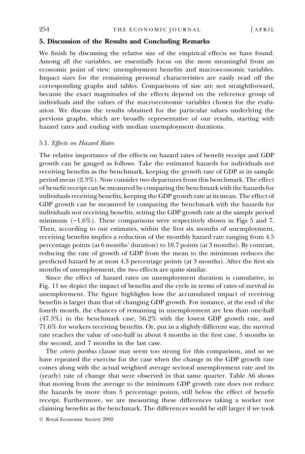
5. Discussion of the Results and Concluding Remarks

We finish by discussing the relative size of the empirical effects we have found.Among all the variables, we essentially focus on the most meaningful from aneconomic point of view: unemployment benefits and macroeconomic variables.Impact sizes for the remaining personal characteristics are easily read off thecorresponding graphs and tables. Comparisons of size are not straightforward,because the exact magnitudes of the effects depend on the reference group ofindividuals and the values of the macroeconomic variables chosen for the evalu-ation. We discuss the results obtained for the particular values underlying theprevious graphs, which are broadly representative of our results, starting withhazard rates and ending with median unemployment durations.

5.1. Effects on Hazard Rates

The relative importance of the effects on hazard rates of benefit receipt and GDPgrowth can be gauged as follows. Take the estimated hazards for individuals notreceiving benefits as the benchmark, keeping the growth rate of GDP at its sampleperiod mean (2.3%). Now consider two departures from this benchmark. The effectof benefit receipt can be measured by comparing the benchmark with the hazards forindividuals receiving benefits, keeping the GDP growth rate at its mean. The effect ofGDP growth can be measured by comparing the benchmark with the hazards forindividuals not receiving benefits, setting the GDP growth rate at the sample periodminimum ()1.6%). These comparisons were respectively shown in Figs 5 and 7.Then, according to our estimates, within the first six months of unemployment,receiving benefits implies a reduction of the monthly hazard rate ranging from 4.5percentage points (at 6 months’ duration) to 10.7 points (at 3 months). By contrast,reducing the rate of growth of GDP from the mean to the minimum reduces thepredicted hazard by at most 4.3 percentage points (at 3 months). After the first sixmonths of unemployment, the two effects are quite similar.

Since the effect of hazard rates on unemployment duration is cumulative, inFig. 11 we depict the impact of benefits and the cycle in terms of rates of survival inunemployment. The figure highlights how the accumulated impact of receivingbenefits is larger than that of changing GDP growth. For instance, at the end of thefourth month, the chances of remaining in unemployment are less than one-half(47.3%) in the benchmark case, 56.2% with the lowest GDP growth rate, and71.6% for workers receiving benefits. Or, put in a slightly different way, the survivalrate reaches the value of one-half in about 4 months in the first case, 5 months inthe second, and 7 months in the last case.

The ceteris paribus clause may seem too strong for this comparison, and so wehave repeated the exercise for the case when the change in the GDP growth ratecomes along with the actual weighted average sectoral unemployment rate and its(yearly) rate of change that were observed in that same quarter. Table A6 showsthat moving from the average to the minimum GDP growth rate does not reducethe hazards by more than 5 percentage points, still below the effect of benefitreceipt. Furthermore, we are measuring these differences taking a worker notclaiming benefits as the benchmark. The differences would be still larger if we took



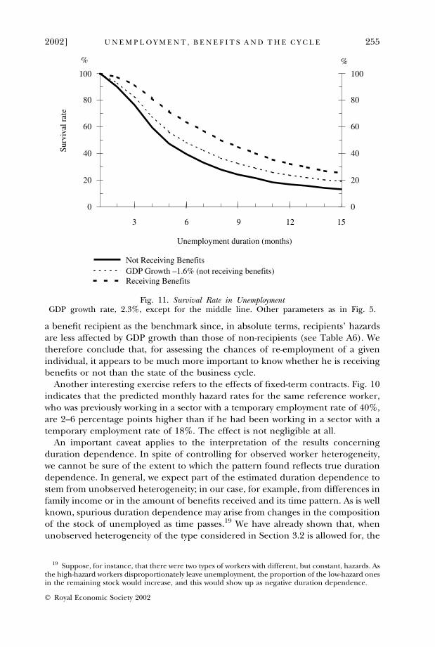
a benefit recipient as the benchmark since, in absolute terms, recipients’ hazardsare less affected by GDP growth than those of non-recipients (see Table A6). Wetherefore conclude that, for assessing the chances of re-employment of a givenindividual, it appears to be much more important to know whether he is receivingbenefits or not than the state of the business cycle.

Another interesting exercise refers to the effects of fixed-term contracts. Fig. 10indicates that the predicted monthly hazard rates for the same reference worker,who was previously working in a sector with a temporary employment rate of 40%,are 2–6 percentage points higher than if he had been working in a sector with atemporary employment rate of 18%. The effect is not negligible at all.

An important caveat applies to the interpretation of the results concerningduration dependence. In spite of controlling for observed worker heterogeneity,we cannot be sure of the extent to which the pattern found reflects true durationdependence. In general, we expect part of the estimated duration dependence tostem from unobserved heterogeneity; in our case, for example, from differences infamily income or in the amount of benefits received and its time pattern. As is wellknown, spurious duration dependence may arise from changes in the compositionof the stock of unemployed as time passes.19 We have already shown that, whenunobserved heterogeneity of the type considered in Section 3.2 is allowed for, the

%

100

80

60

40

20

0

%

100

80

60

40

20

0

Surv

ival

rat

e


Not Receiving BenefitsGDP Growth –1.6% (not receiving benefits)Receiving Benefits

3 6 9 12 15

Fig. 11. Survival Rate in UnemploymentGDP growth rate, 2.3%, except for the middle line. Other parameters as in Fig. 5.

19 Suppose, for instance, that there were two types of workers with different, but constant, hazards. Asthe high-hazard workers disproportionately leave unemployment, the proportion of the low-hazard onesin the remaining stock would increase, and this would show up as negative duration dependence.



estimated effects of the key variables of interest do not vary much. Nevertheless,the basic identification problem remains. As a result, more attention should bepaid to the exit rates in the first few months, since they are based on a morerepresentative sample. For the same reason, we prefer not to put much emphasison the disparity between the shapes of duration dependence found in the data andthose predicted by the standard search model.

5.2. Effects on Median Unemployment Duration

What policy implications can be drawn from our results? Surely, the policy goalshould be to reduce the unemployment rate, rather than increasing jobfindingrates per se. However, Spanish unemployment is, as in many other Europeancountries, chiefly an outflow problem. This has manifested itself in a large share oflong-term unemployment. These facts make a prima facie case for policy measuresaimed at increasing re-employment probabilities.

A way to show the implications from our results is to assess the differential impactover the business cycle of policies aimed at reducing unemployment durationthrough reductions in benefit entitlements. We have already shown that, at three orfour months into the spell, the exit rates of workers without benefits are twice as largeas those of workers with benefits, and the difference is statistically very significant.

Now, under the restrictive assumptions of the two-regime model introduced inSection 3.1, we can integrate these hazard rates to obtain approximate mediandurations of unemployment spells. The results are summarised in Table 5. Ourdata are, in fact, best suited to providing information on the effects of experi-menting with the most extreme policy of all: eliminating benefits altogether. Thetable indicates that such an extreme measure would have sizable effects on medianunemployment duration.20 It also shows that, for long durations, there are largereffects of benefits in an expansion than in a recession. So, for example, reducingthe benefit entitlement from 12 to 8 months has no effect in a recession but itimplies a 4-month reduction in median unemployment in an expansion.

Policy decisions, however, should be based on welfare assessments, and it is notobvious that reducing benefit duration would necessarily increase welfare. Un-employment benefits create both gains and losses. The former come in the form ofsmoother consumption of households with unemployed members (in the pres-ence of risk aversion and incomplete private insurance against the unemploymentrisk) and of more efficient worker-firm matches.21 The losses, apart from longerunemployment duration and the potential resulting loss of human capital, mayarise from lower precautionary saving, leading to lower capital stock and output. Asa result, the net welfare impact of a change in benefit duration would be difficultto assess, and no established evidence is yet available (Valdivia, 1995; Hopenhaynand Nicolini, 1997). What our results show is that the desirable effects of benefits

20 Note that lowering benefit duration may not only raise hazard rates from unemployment but mayalso lower hazard rates into unemployment (not analysed here), although the international empiricalevidence suggests that this effect is relatively small (Atkinson and Micklewright, 1991).

21 Gruber (1997) provides empirical evidence on the consumption smoothing role of unemploymentbenefits in the USA.



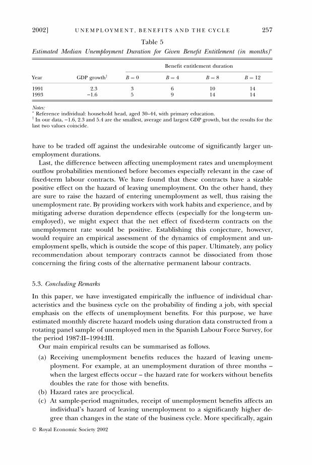
have to be traded off against the undesirable outcome of significantly larger un-employment durations.

Last, the difference between affecting unemployment rates and unemploymentoutflow probabilities mentioned before becomes especially relevant in the case offixed-term labour contracts. We have found that these contracts have a sizablepositive effect on the hazard of leaving unemployment. On the other hand, theyare sure to raise the hazard of entering unemployment as well, thus raising theunemployment rate. By providing workers with work habits and experience, and bymitigating adverse duration dependence effects (especially for the long-term un-employed), we might expect that the net effect of fixed-term contracts on theunemployment rate would be positive. Establishing this conjecture, however,would require an empirical assessment of the dynamics of employment and un-employment spells, which is outside the scope of this paper. Ultimately, any policyrecommendation about temporary contracts cannot be dissociated from thoseconcerning the firing costs of the alternative permanent labour contracts.

5.3. Concluding Remarks

In this paper, we have investigated empirically the influence of individual char-acteristics and the business cycle on the probability of finding a job, with specialemphasis on the effects of unemployment benefits. For this purpose, we haveestimated monthly discrete hazard models using duration data constructed from arotating panel sample of unemployed men in the Spanish Labour Force Survey, forthe period 1987:II–1994:III.

Our main empirical results can be summarised as follows.

(a) Receiving unemployment benefits reduces the hazard of leaving unem-ployment. For example, at an unemployment duration of three months –when the largest effects occur – the hazard rate for workers without benefitsdoubles the rate for those with benefits.

(b) Hazard rates are procyclical.(c) At sample-period magnitudes, receipt of unemployment benefits affects an

individual’s hazard of leaving unemployment to a significantly higher de-gree than changes in the state of the business cycle. More specifically, again

Table 5

Estimated Median Unemployment Duration for Given Benefit Entitlement (in months)�

Benefit entitlement duration

Year GDP growthy B ¼ 0 B ¼ 4 B ¼ 8 B ¼ 12

1991 2.3 3 6 10 141993 )1.6 5 9 14 14

Notes:� Reference individual: household head, aged 30–44, with primary education.y In our data, )1.6, 2.3 and 5.4 are the smallest, average and largest GDP growth, but the results for thelast two values coincide.



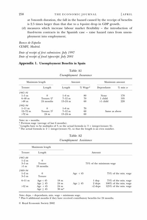
at 3-month duration, the fall in the hazard caused by the receipt of benefitsis 2.5 times larger than that due to a 4-point drop in GDP growth.

(d) measures which increase labour market flexibility – the introduction offixed-term contracts in the Spanish case – raise hazard rates from unem-ployment into employment.

Banco de Espan~aCEMFI, Madrid.

Date of receipt of first submission: July 1997Date of receipt of final typescript: July 2001

Appendix 1. Unemployment Benefits in Spain

Table A1

Unemployment Insurance

Maximum length Amount Maximum amount

Tenure Length Length % Wage* Dependants % min w

1987–911–5 m 0 1–6 m 80 None 1706–48 m Tenure/2y 7–12 m 70 1 child 195>48 m 24 months 13–24 m 60 >1 child 220

1992–941–11 m 0 1–6 m 7012–72 m Tenure/3z 7–12 m 60 Same as above>72 m 24 m 13–24 m 60

Notes: m = months.* Previous wage (average of last 6 months).y Lengths have to be multiples of 3, so the actual formula is: 3 � integer(tenure/6).z The actual formula is: 2 � integer(tenure/6), so that the length is an even number.

Table A2

Unemployment Assistance

Maximum length

Tenure Length Amount

1987–881–2 m 03–5 m Tenure 75% of the minimum wage>5 m 18 months

1989–941–2 m 0 Age < 45 75% of the min. wage3–5 m Tenure

6–11 m Age < 45 18 m 1 dep 75% of the min. wageAge � 45 24 m Age � 45 2 deps 100% of the min. wage

>12 m Age < 45 24 m >2 deps 125% of the min. wageAge � 45 30 m*

Notes: deps. = dependants, min. wage = minimum wage.* Plus 6 additional months if they have received contributory benefits for 24 months.



Appendix 2. Database description

A2.1. Individual Data

Source. Rotating panel from the Spanish Labour Force Surveys (Encuesta de PoblacionActiva: Estadıstica de Flujos) from 1987:II to 1994:III, provided by the National StatisticalOffice (Instituto Nacional de Estadıstica, INE).Sample. From a sample of men of 20–64 years of age, we exclude those

• in the military or the substitute civil service• always employed during the observed period• never in the labour force during the observed period• observed only once• with a missing interview between two valid interviews• who have never worked and are not looking for work• who are full-time students (from the moment they become so)• employed who do not answer the question about how long they have been in their

current job• unemployed (and those not in the labour force) who answer neither the question ‘How

long has it been since your last job?’ nor the question ‘How long have you been lookingfor a job?’

• unemployed who do not answer the question about their relation with the publicemployment office (INEM)

• unemployed for over eight years.

60,036 unemployment spells satisfy these restrictions. Restricting the sample to thoseunemployed observed when entering unemployment leaves 27,382 spells of unemployment.Finally, at the estimation stage, we drop 376 spells (1.37%) for which the information oneconomic sector at the previous job is lacking.

Unemployment duration. Both the unemployment and the benefit duration variables aremeasured in months, the smallest unit allowed by the data. The length of unemployment

Table A3

Calendar of Unemployment Benefit Reforms in Spain, 1987–94

� March 1989: More generous assistance system established for the unemployed aged 45 or older interms of the duration and the amount of benefits. Unemployed workers aged at least 52 years old whohave fulfilled all requirements for obtain a retirement pension except for the minimum age, may drawbenefits until retirement age.

�November 1990: Reform to make the special unemployment benefit system for underemployed workers inagriculture in two regions (Andalucıa and Extremadura) more similar to the general assistancesystem.

� April 1992: Reduction in the generosity of contributory benefits in terms of the the duration and theamount of benefits. The option of receiving the full amount of unemployment benefit entitlement inone instalment so as to set up a business is severely limited.

� February 1993: Unemployment benefits become taxable income (as from January 1994). The minimumamount for contributory benefits is lowered from 100% ot 75% of the minimum wage. Assistancebenefits:

(a) The amount of assistance benefits becomes proportional to hours worked, in the case of part-time workers.

(b) Explicit definition of dependants: spouse, children below 26 years old, and disabled children, aslong as their income is below 75% of the minimum wage.

(c) Income per family member cannot be above 75% of the minimum wage (before it was 100%).

The unemployed worker drawing benefits must, within a 5-day period, show proof of having visited firmsoffering him/her a job through the employment office.



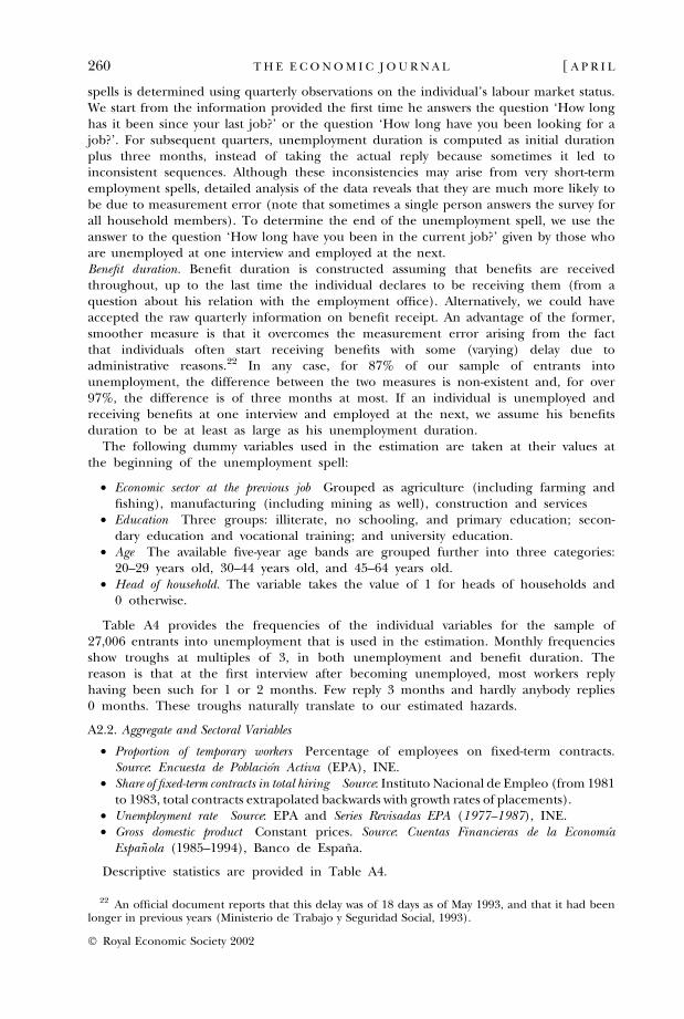
spells is determined using quarterly observations on the individual’s labour market status.We start from the information provided the first time he answers the question ‘How longhas it been since your last job?’ or the question ‘How long have you been looking for ajob?’. For subsequent quarters, unemployment duration is computed as initial durationplus three months, instead of taking the actual reply because sometimes it led toinconsistent sequences. Although these inconsistencies may arise from very short-termemployment spells, detailed analysis of the data reveals that they are much more likely tobe due to measurement error (note that sometimes a single person answers the survey forall household members). To determine the end of the unemployment spell, we use theanswer to the question ‘How long have you been in the current job?’ given by those whoare unemployed at one interview and employed at the next.Benefit duration. Benefit duration is constructed assuming that benefits are receivedthroughout, up to the last time the individual declares to be receiving them (from aquestion about his relation with the employment office). Alternatively, we could haveaccepted the raw quarterly information on benefit receipt. An advantage of the former,smoother measure is that it overcomes the measurement error arising from the factthat individuals often start receiving benefits with some (varying) delay due toadministrative reasons.22 In any case, for 87% of our sample of entrants intounemployment, the difference between the two measures is non-existent and, for over97%, the difference is of three months at most. If an individual is unemployed andreceiving benefits at one interview and employed at the next, we assume his benefitsduration to be at least as large as his unemployment duration.

The following dummy variables used in the estimation are taken at their values atthe beginning of the unemployment spell:

• Economic sector at the previous job Grouped as agriculture (including farming andfishing), manufacturing (including mining as well), construction and services

• Education Three groups: illiterate, no schooling, and primary education; secon-dary education and vocational training; and university education.

• Age The available five-year age bands are grouped further into three categories:20–29 years old, 30–44 years old, and 45–64 years old.

• Head of household. The variable takes the value of 1 for heads of households and0 otherwise.

Table A4 provides the frequencies of the individual variables for the sample of27,006 entrants into unemployment that is used in the estimation. Monthly frequenciesshow troughs at multiples of 3, in both unemployment and benefit duration. Thereason is that at the first interview after becoming unemployed, most workers replyhaving been such for 1 or 2 months. Few reply 3 months and hardly anybody replies0 months. These troughs naturally translate to our estimated hazards.

A2.2. Aggregate and Sectoral Variables

• Proportion of temporary workers Percentage of employees on fixed-term contracts.Source: Encuesta de Poblacion Activa (EPA), INE.

• Share of fixed-term contracts in total hiring Source: Instituto Nacional de Empleo (from 1981to 1983, total contracts extrapolated backwards with growth rates of placements).

• Unemployment rate Source: EPA and Series Revisadas EPA (1977–1987), INE.• Gross domestic product Constant prices. Source: Cuentas Financieras de la Economıa

Espan~ola (1985–1994), Banco de Espana.

Descriptive statistics are provided in Table A4.

22 An official document reports that this delay was of 18 days as of May 1993, and that it had beenlonger in previous years (Ministerio de Trabajo y Seguridad Social, 1993).



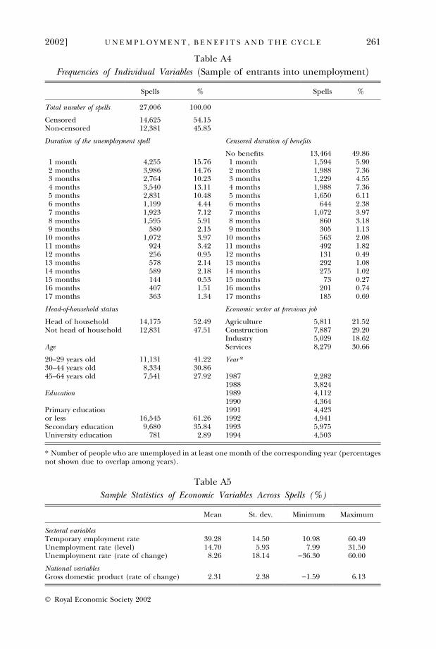
Table A4

Frequencies of Individual Variables ðSample of entrants into unemploymentÞ

Spells % Spells %

Total number of spells 27,006 100.00

Censored 14,625 54.15Non-censored 12,381 45.85

Duration of the unemployment spell Censored duration of benefits

No benefits 13,464 49.861 month 4,255 15.76 1 month 1,594 5.902 months 3,986 14.76 2 months 1,988 7.363 months 2,764 10.23 3 months 1,229 4.554 months 3,540 13.11 4 months 1,988 7.365 months 2,831 10.48 5 months 1,650 6.116 months 1,199 4.44 6 months 644 2.387 months 1,923 7.12 7 months 1,072 3.978 months 1,595 5.91 8 months 860 3.189 months 580 2.15 9 months 305 1.13

10 months 1,072 3.97 10 months 563 2.0811 months 924 3.42 11 months 492 1.8212 months 256 0.95 12 months 131 0.4913 months 578 2.14 13 months 292 1.0814 months 589 2.18 14 months 275 1.0215 months 144 0.53 15 months 73 0.2716 months 407 1.51 16 months 201 0.7417 months 363 1.34 17 months 185 0.69

Head-of-household status Economic sector at previous job

Head of household 14,175 52.49 Agriculture 5,811 21.52Not head of household 12,831 47.51 Construction 7,887 29.20

Industry 5,029 18.62Age Services 8,279 30.66

20–29 years old 11,131 41.22 Year *30–44 years old 8,334 30.8645–64 years old 7,541 27.92 1987 2,282

1988 3,824Education 1989 4,112

1990 4,364Primary education 1991 4,423or less 16,545 61.26 1992 4,941Secondary education 9,680 35.84 1993 5,975University education 781 2.89 1994 4,503

* Number of people who are unemployed in at least one month of the corresponding year (percentagesnot shown due to overlap among years).

Table A5

Sample Statistics of Economic Variables Across Spells (%)

Mean St. dev. Minimum Maximum

Sectoral variablesTemporary employment rate 39.28 14.50 10.98 60.49Unemployment rate (level) 14.70 5.93 7.99 31.50Unemployment rate (rate of change) 8.26 18.14 )36.30 60.00

National variablesGross domestic product (rate of change) 2.31 2.38 )1.59 6.13



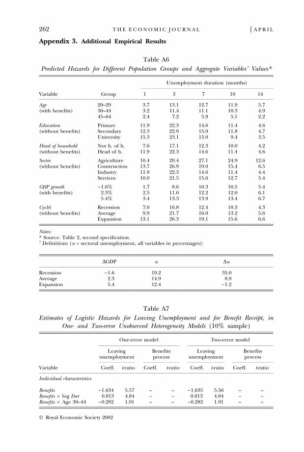
Appendix 3. Additional Empirical Results

Table A6

Predicted Hazards for Different Population Groups and Aggregate Variables’ Values*


Variable Group 1 3 7 10 14

Age 20–29 3.7 13.1 12.7 11.9 5.7(with benefits) 30–44 3.2 11.4 11.1 10.3 4.9

45–64 2.4 7.2 5.9 5.1 2.2

Education Primary 11.9 22.3 14.6 11.4 4.6(without benefits) Secondary 12.3 22.9 15.0 11.8 4.7

University 15.3 23.1 13.0 9.4 3.5

Head of household Not h. of h. 7.6 17.1 12.3 10.0 4.2(without benefits) Head of h. 11.9 22.3 14.6 11.4 4.6

Sector Agriculture 10.4 29.4 27.1 24.9 12.6(without benefits) Construction 13.7 26.9 19.0 15.4 6.5

Industry 11.9 22.3 14.6 11.4 4.4Services 10.0 21.5 15.6 12.7 5.4

GDP growth )1.6% 1.7 8.6 10.3 10.5 5.4(with benefits) 2.3% 2.5 11.0 12.2 12.0 6.1

5.4% 3.4 13.3 13.9 13.4 6.7

Cycley Recession 7.0 16.8 12.4 10.3 4.3(without benefits) Average 9.9 21.7 16.0 13.2 5.6

Expansion 13.1 26.3 19.1 15.6 6.6

Notes:* Source: Table 2, second specification.y Definitions (u = sectoral unemployment, all variables in percentages):

DGDP u Du

Recession )1.6 19.2 35.0Average 2.3 14.9 8.9Expansion 5.4 12.4 )1.2

Table A7

Estimates of Logistic Hazards for Leaving Unemployment and for Benefit Receipt, inOne- and Two-error Unobserved Heterogeneity Models (10% sample)

One-error model Two-error model

Leavingunemployment

Benefitsprocess

Leavingunemployment

Benefitsprocess

Variable Coeff. t-ratio Coeff. t-ratio Coeff. t-ratio Coeff. t-ratio

Individual characteristics

Benefits )1.634 5.57 – – )1.635 5.56 – –Benefits � log Dur 0.813 4.84 – – 0.813 4.84 – –Benefits � Age 30–44 )0.282 1.91 – – )0.282 1.91 – –



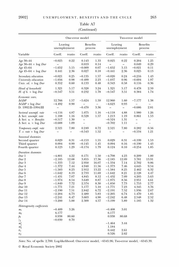
Table A7

(Continued)

One-error model Two-error model

Leavingunemployment

Benefitsprocess

Leavingunemployment

Benefitsprocess

Variable Coeff. t-ratio Coeff. t-ratio Coeff. t-ratio Coeff. t-ratio

Age 30–44 )0.025 0.22 0.143 1.33 0.025 0.22 0.204 1.25Age 30–44 � log Dur – 0.019 0.14 – – 0.049 0.29Age 45–64 )1.652 5.15 )0.009 0.07 )1.652 5.15 )0.021 0.11Age 45–64 � log Dur 0.441 2.36 0.027 0.18 )0.441 2.36 0.025 0.13

Secondary education )0.021 0.25 )0.135 1.57 )0.020 0.24 )0.216 1.43University education )1.056 0.98 )0.499 2.23 )1.037 0.96 )0.694 1.97Univ. ed. � log Dur 0.352 0.60 0.133 0.48 0.343 0.58 0.116 0.36

Head of household 1.321 5.17 0.328 3.24 1.321 5.17 0.478 2.59H. of h. � log Dur )0.547 3.51 0.232 1.78 )0.547 3.51 0.384 1.74

Economic vars.DGDP 12.766 1.57 )5.624 1.59 12.960 1.60 )7.177 1.38DGDP � log Dur )4.492 0.90 – – )4.623 0.93 – –D. 1992:II–1994:III – )0.470 3.36 – – )0.686 2.81

Sectoral unempl. rate )4.116 4.87 1.075 1.16 )4.118 4.88 1.980 1.26D Sect. unempl. rate 1.188 1.16 0.528 1.57 1.213 1.19 0.861 1.53D Sect. u. � Benefits )0.517 1.30 – )0.524 1.31 – –D Sect. u. � log Dur )0.688 1.09 – )0.702 1.11 – –

Temporary empl. rate 2.521 7.80 0.249 0.72 2.521 7.80 0.282 0.56T. e. rate � log Dur – – )0.543 1.52 – – )0.534 1.21

Seasonal dummiesSecond quarter 0.029 0.31 )0.153 1.55 0.029 0.31 )0.199 1.53Third quarter 0.094 0.99 )0.145 1.45 0.094 0.16 )0.190 1.43Fourth quarter 0.123 1.29 )0.174 1.79 0.124 0.10 )0.254 1.85

Duration dummiesDur 1 )4.801 4.22 0.171 1.50 )4.798 4.23 0.209 1.00Dur 2 )2.185 12.08 3.855 17.36 )2.185 12.09 3.781 13.91Dur 3 )1.333 7.12 2.950 16.07 )1.334 7.14 2.702 9.86Dur 4 )1.372 7.44 4.940 11.56 )1.373 7.46 4.645 9.54Dur 5 )1.583 8.23 2.912 13.22 )1.584 8.25 2.462 6.32Dur 6 )1.642 8.19 2.733 11.69 )1.642 8.21 2.128 4.47Dur 7 )1.431 7.07 4.845 8.12 )1.432 7.09 4.205 5.63Dur 8 )1.974 8.54 3.649 8.87 )1.975 8.56 2.951 4.61Dur 9 )1.849 7.72 2.574 8.30 )1.850 7.73 1.753 2.77Dur 10 )1.771 7.21 5.177 5.10 )1.771 7.23 4.345 3.76Dur 11 )2.190 7.51 2.842 6.72 )2.191 7.52 1.936 2.67Dur 12 )2.204 6.73 2.489 5.83 )2.205 6.74 1.470 1.85Dur 13 )2.241 6.47 3.603 4.90 )2.242 6.48 2.548 2.52Dur 14 )3.200 5.88 2.309 4.57 )3.199 5.89 1.185 1.32

Heterogeneity coefficientsm1 )0.409 3.26 )0.408 3.01m2 6.177 6.177p1 0.938 80.60 0.938 80.68c2 )0.030 0.70m�

1 )1.464 3.44m�

2 1.184p1 0.442 2.61p2 0.526 2.62

Notes: No. of spells: 2,700. Log-likelihood: One-error model, )6545.96; Two-error model, )6545.39.



References

Ahn, N. and Ugidos, A. (1995). ‘Duration of unemployment in Spain: relative effects ofunemployment benefit and family characteristics’, Oxford Bulletin of Economics and Statistics,vol. 57, pp. 249–64.

Alba-Ramirez, A. and Freeman, R. (1990). ‘Jobfinding and wages when longrun unemployment isreally long: the case of Spain’, NBER Working Paper 3409. Cambridge, MA: NBER.

Andres, J. and Garcıa, J. (1993). ‘Los determinantes de la probabilidad de abandonar eldesempleo: evidencia empırica para el caso espanol’, mimeo, Universidad de Valencia.

Atkinson, A. and Micklewright, J. (1991). ‘Unemployment compensation and labor markettransitions: a critical review’, Journal of Economic Literature, vol. 29, pp. 1679–727.

Bentolila, S. and Dolado, J. (1994). ‘Labour flexibility and wages: lessons from Spain’, EconomicPolicy, vol. 18, pp. 53–99.

Blanchard, O. and Diamond, P. (1990). ‘The cyclical behavior of the gross flows of U.S. workers’,Brookings Papers on Economic Activity, vol. 2, pp. 85–155.

Blanchard, O. and Diamond, P. (1994). ‘Ranking, unemployment duration, and wages’, Review ofEconomic Studies, vol. 61, pp. 417–34.

Blanco, J. (1995). ‘La duracion del desempleo en Espana’, in ( J. Dolado and J. Jimeno, eds),Estudios sobre el Funcionamiento del Mercado de Trabajo Espanol. Madrid: Fundacion de Estudiosde Economıa Aplicada.

Bover, O., Arellano, M. and Bentolila, S. (1996). ‘Unemployment duration, benefit duration, andthe business cycle’, Estudios Economicos no. 57. Madrid: Banco de Espana.

Burdett, K. (1981). ‘A useful restriction on the offer distribution in job search models’, in(G. Eliasson, B. Holmlund and F. Stafford, eds), Studies in Labor Market Behavior: Sweden andthe United States. Stockholm: IUI Conference Report.

Cebrian, I., Garcıa, C., Muro, J., Toharia, L. and Villagomez, E. (1995). ‘Prestaciones pordesempleo, duracion y recurrencia del paro’, in (J. Dolado and J. Jimeno, eds), Estudios sobreel Funcionamiento del Mercado de Trabajo Espanol. Madrid: Fundacion de Estudios de EconomiaAplicada.

Gritz, R. and MaCurdy, T. (1989). ‘The influence of unemployment insurance on theunemployment experiences of young workers’, mimeo, Stanford University.

Gruber, J. (1997). ‘The consumption smoothing benefits of unemployment insurance’, AmericanEconomic Review, vol. 87, pp. 192–205.

Ham, J. and LaLonde, R. (1996). ‘The effect of sample selection and initial conditions in durationmodels: evidence from experimental data on training’, Econometrica, vol. 64, pp. 175–205.

Heckman, J. and Singer, B. (1984). ‘A method for minimizing the distributional assumptions ineconometric models for duration data’, Econometrica, vol. 52, pp. 271–320.

Hopenhayn, H. and Nicolini, J. P. (1997). ‘Optimal unemployment insurance’, Journal of PoliticalEconomy, vol. 105, pp. 412–38.

Imbens, G. and Lynch, L. (1993). ‘Re-employment probabilities over the business cycle’, NBERWorking Paper 4585. Cambridge, MA: NBER.

Jenkins, S. (1995). ‘Easy estimation methods for discrete-time duration models’, Oxford Bulletin ofEconomics and Statistics, vol. 57, pp. 120–38.

Katz, L. and Meyer, B. (1990). ‘The impact of potential duration of unemployment benefits onthe duration of unemployment’, Journal of Public Economics, vol. 41, pp. 45–72.

Kiefer, N. (1987). ‘Analysis of grouped duration data’, Cornell CAE Working Paper 87–12.Lancaster, T. (1990). The Econometric Analysis of Transition Data, Cambridge: Cambridge University

Press.Lancaster, T. and Nickell, S. (1980). ‘The analysis of re-employment probabilities for the

unemployed’, Journal of the Royal Statistic Society, vol. 143, pp. 141–52.Layard, R., Nickell, S. and Jackman, R. (1991). Unemployment, Macroeconomic Performance and the

Labor Market, Oxford: Oxford University Press.Manski, C. (1993). ‘Identification of endogenous social effects: the reflection problem’, Review of

Economic Studies, vol. 60, pp. 531–42.Meghir, C. and Whitehouse, E. (1997). ‘Labour market transitions and retirement of men in the

UK’, Journal of Econometrics, vol. 79, pp. 327–54.Meyer, B. (1990). ‘Unemployment insurance and unemployment spells’, Econometrica, vol. 58,

pp. 757–82.Ministerio de Trabajo y Seguridad Social (1993). ‘Prestaciones por desempleo’, mimeo.Moffit, R. and Nicholson, W. (1982). ‘The effect of unemployment insurance on unemployment:

the case of federal supplemental benefits’, Review of Economics and Statistics, vol. 64, pp. 1–11.Mortensen, D. (1977). ‘Unemployment insurance and job search decisions’, Industrial and Labor

Relations Review, vol. 30, pp. 505–17.



Narendranathan, W. and Stewart, M. (1993). ‘How does the benefit effect vary as unemploymentspells lengthen?’, Journal of Applied Econometrics, vol. 8, pp. 361–81.

Narendranathan, W., Nickell, S. and Stern, J. (1985). ‘Unemployment benefits revisited’, ECONOMIC

JOURNAL, vol. 95, pp. 307–29.Sueyoshi, G. (1995). ‘A class of binary response models for grouped duration data’, Journal of

Applied Econometrics, vol. 10, pp. 411–31.Toharia, L. (1997). ‘El sistema espanol de proteccion por desempleo’, Papeles de Economıa Espan~ola,

no. 72, pp. 192–213.Valdivia, H. (1995). ‘Evaluating the welfare benefits of unemployment insurance’, mimeo,

Northwestern University.



Documents

THE ECONOMIC JOURNAL - CEMFIarellano/EJpapBAB.pdf* We wish to thank Daron Acemoglu, Alfonso Alba, Olivier Blanchard, Raquel Carrasco, Daniel Cohen, Jaume Garcı´a, Guido Imbens, Juan