The economic lot scheduling problem with deteriorating

ORIGINAL ARTICLE

The economic lot scheduling problem with deteriorating itemsand shortage: an imperialist competitive algorithm

V. Kayvanfar & M. Zandieh

Received: 19 October 2010 /Accepted: 28 November 2011# Springer-Verlag London Limited 2012

Abstract This paper addresses an economic lot schedulingproblem (ELSP) for manufacturing environments regardingslack costs and deteriorating items using the extended basicperiod approach under Power-of-Two (PoT) policy. Thepurpose of this research is to determine an optimal batchsize for a product and minimizing total related costs to sucha problem. The cost function consists of three components,namely, setup cost, holding cost includes deteriorating fac-tor, and slack cost. The ELSP is concerned with the sched-uling decision of n items and lot sizing. Avoiding scheduleinterference is the main problem in ELSP. The used PoTpolicy ensures that the replenishment cycle of each item tobe integer and this task reduces potential schedule interfer-ences. Since the ELSP is shown as an NP-hard problem, animperialist competitive algorithm is employed to providegood solutions within reasonable computational times.Computational results show that the proposed approachcan efficiently solve such complicated problems.

Keywords Economic lot scheduling problem . Deteriorationfactor . Shortage cost . Imperialist competitive algorithm

1 Introduction

Scheduling the production of several products on a singlefacility with the objective of reducing the sum of holdingcosts and setup costs has been studied in the literature asformal analysis since 1950s as economic lot schedulingproblem (ELSP). The ELSP merges lot sizing and produc-tion scheduling decisions and is one of the most represen-tative topics. The optimal solution to this problem is knownto be quite difficult. The conventional ELSP is concernedwith the scheduling of cyclical production of two or morethan two products on a single facility in which lots aredifferent in size and consequently are different in productiontimes and cycles, over an infinite planning horizon, assum-ing deterministic demand for each product. On the otherhand, the conventional ELSP is defined as the problem offinding the production sequence, production times, and idletimes of several products in a single facility in a cyclicschedule so that the demands are made without stock-outsor backorders and average inventory holding and setup costsare minimized [31].

In this research, we present a model including dete-rioration factor and slack cost. In real world and inmany industries, deterioration occurs for a lot of itemssuch as food industries. Soman et al. [37] showed thatin these industries, products do have limited shelf lifethat restricts the amount of inventory that can be carriedwithout spoilage. Actually, products must have limitedstoring life because of decreasing the quality of prod-ucts or deterioration.

The ELSP occurs when one machine is used to meetdeterministic and fixed demand of several products over aninfinite horizon. Also, the issue of batching arises because thesystem usually requires a setup cost and a setup time when a

V. KayvanfarDepartment of Industrial Engineering,Mazandaran University of Science and Technology,Babol, Iran

M. Zandieh (*)Department of Industrial Management, Management andAccounting Faculty, Shahid Beheshti University, G.C.,Tehran, Irane-mail: [email protected]

V. KayvanfarResearch Institute of Food Science and Technology,P.O. Box 91735-139, Mashhad, Iran

Int J Adv Manuf TechnolDOI 10.1007/s00170-011-3820-6

machine switches from one product to the next. In addition tothe discrete parts manufacturing, multi-products or multi-purpose processors are common features in many chemicalplants such as those producing pharmaceuticals, biochemical,polymers, cosmetics, food, and beverages, etc. Therefore, anymethodology for solving the ELSP has huge potential ofapplicability for industry [21]. Of another potential, lot sizingapplications can be applied to high technology industries.Storerooms, which employ automated storage and retrievalsystems, supply numerous electronic components, in a spec-ified mix, to circuit-board assembly lines [27]. The rawmaterial is a further usage of ELSP which leads to inventoryholding costs. In most cases, the raw materials represent amajor part of the cost of the finished product and forsakingthese can lead to ineffective policies; for instance, injectionmolding of plastic parts, such as panels and fixtures in auto-mobiles, refrigerators, or consumer electronics. Another ex-ample in such area arises where the raw material is producedinternally at a finite rate in the packaging of liquid medicalproducts. The pharmaceutical industry employs commonmachines to bottle and package different products, and thebottled products are the finished items [17].

To the best of the authors' knowledge, there is no otherstudy that directly survey the conventional ELSP model thatincludes both the deterioration factor and slack cost; how-ever, Yao and Huang [43] presented an ELSP model includ-ing deteriorating factor. A production plan in the ELSPschedules the items within “basic periods,” where a basicperiod (BP) is an interval of time that consists of setup andproduction of a subset (or all) of the products [41]. Thesolution of the ELSP is usually given in terms of a set ofmultipliers {ki}; i01, 2,…, n and the BP in which eachproduct is produced. The BPs in the ELSP can be catego-rized as either the “BP” or the “extended basic period”(EBP) approach. The BP approach assumes that the produc-tion runs of all products must be made in each BP and thisBP must be long enough to accommodate the production ofall the products. The researchers have demonstrated that theELSP under the EBP approach, denoted as the ELSP (EBP),always yields better solutions [14]. In the literature, chang-ing the policy of resolving from the BP approach to the EBPapproach is for eliminating the wasted capacity of the pro-duction facility due to the restrictive feasibility condition.Using of this approach causes that the BPs are not equallyloaded. Consequently, minimizing the maximal load on anyBP is another objective as well as the feasibility and theobjective of minimizing the total operating cost, because itleads to smaller BPs and consequently lower cost.

Since Hsu [22] has shown that even in the absence ofsetup costs this problem is NP-hard, if for instance, oneemploys some branch-and-bound (B&B) algorithm or otherdeterministic and optimum algorithms, for solving suchscheduling problem, the search could be computationally

expensive since there may be many intermediate sets ofbasic periods and their corresponding multipliers K(B) thatneed to be tested for feasibility, or for which one must obtaina feasible production schedule. Now there is a problem, andthat is misinforming the search by using some greedy algo-rithms which is caused by quality of the obtained solutionsin solving such scheduling problem which consequentlysearch process mislead by misjudging the feasibility of anintermediate set of K(B) at a particular BP. So, a “reliableheuristic” that compromises between optimality and com-putational efficiency is needed.

The power-of-two (PoT) policy necessitates that ki02q;

q≥0 integer, for all ki in the set of multipliers K(B). On theother hand, the multipliers are restricted to be PoT. Thispolicy recently became popular for lot scheduling problemsbecause it reduces potential interferences. There are a lot ofreasons in support of the acceptance of the PoT policy.Under PoT policy, researchers were able to derive someeasy and effective heuristics to solve both incapacitatedand capacitated lot sizing problems. It is interesting thatthe worst case bounds for PoT policy are actually reason-ably tight [41]. Also, implementing the replenishment strat-egies under PoT policy for decision makers is easier thanother policies.

In this paper, an imperialist competitive algorithm(ICA) is proposed to Slack-Deter-ELSP (EBP-PoT).The paper has following structure. Section 2 gives lit-erature review of conventional ELSP with and withoutdifferent policies. Section 3 includes problem descrip-tion. Section 4 introduces the proposed ICA. Section 5explains genetic algorithm (GA) implementation for ourproblem. Section 6 describes how to generate a feasiblesolution to our problem. Section 7 presents experimentaldesign. Section 8 includes experimental results achievedby proposed ICA which have been compared thoseachieved by past GA. Finally, Section 9 consists ofconclusions and future work.

2 Literature review

In this section, we will review the literature of ELSP withand without different kinds of policies.

As pointed out in previous section, ELSP is concernedwith the scheduling of the cyclical production of n≥2 itemson a single facility in batches that are different in size andconsequently different in production time and cycle. InELSP, the major problem is how to avoid schedule inter-ference and ensure that there is enough time available tosetup and produce the lots selected to meet demands untilthe next production run. Soman et al. [38] proposed amodel which allow products to be produced more thanonce in a cycle and also do not allow reducing production

Int J Adv Manuf Technol

rate. Also, Brander and Segerstedt [8] modified the tradi-tional cost function to include not only setup and inventoryholding cost but also a time variable cost for operating theproduction facility.

In cyclic approaches, main alternatives are the commoncycle (CC) introduced by Eilon [13], extended by Maxwell[28], the BP approach, developed by Bomberger [7] and theextended basic period, introduced by Elmaghraby [14]. Inthe former, each product is produced once in a CC and in thesame cycle time, which is continuously repeated.

The BP approach, which was developed by Bomberger[7], assumes that production runs of all products shall bemade in each basic period. In this approach there is a singleBP, B, and each item is a replenishment cycle, Ti, is aninteger multiple of B, namely, Ti0ki×B. In this manner, theproblem objective will be finding a set of coefficients,{k1,k2, k3,…, kN}, instead of finding a set of replenishmentcycles {T1, T2, T3,…, TN}. This approach ensures sequencefeasibility by means of requiring a basic cycle long enoughto accommodate production of all items once. In the litera-ture, Cooke et al. [11] proposed a relatively simple MIPformulation for the ELS problem that creates a completeschedule, assuming a basic period value and productionfrequencies that have been predetermined.

The EBP expands upon the BP by allowing different cycletimes for different products. Namely, by utilizing two consec-utive fundamental cycles, but making them an integer multi-ple, ki (for ith product), of some BP, long enough toaccommodate a production run of all products. It has beenfound that the EBP approach is superior to the BP in respect ofcosts minimization, very significantly so in some cases. How-ever, it tends to have much longer rotation cycle times. Thereis an extensive literature on this subject by referring toElmaghraby [14] and Lopez and Kingsman [26].

In PoT policy, as pointed out earlier, it is assumed thatki02

q; q≥0 integer, for all ki in the set of multipliers K(B). Aspecial case of the ELSP which assumes that the capacity ofthe production facility is defined by the annual availablesetup time is presented by Roundy [36]. Another specialcase of ELSP is studied by Jackson et al. [24] on the jointreplenishment problem, where the capacity of the produc-tion facility is unlimited. Also, Federgruen and Zheng [16]use “unrestricted and stationary PoT policies” for multistageproduction and inventory systems.

In the lot sizing problems, if the deterioration of the itemsis ignored the demand may not be met. So it may causeadditional costs due to shortage. A new inventory model inwhich products deteriorate at a constant rate and in whichdemand, production rates are allowed to vary with time hasbeen introduced by Balkhi and Benkherouf [5]. In thismodel, an optimal production policy that minimizes the totalrelevant cost is established. Totally, most of the inventorymodels that considered the deteriorating factor are one-item

models; for example, Misra [29], Elsayed and Teresi [15],Heng et al. [20], and Abad [1,2].

There are some classifications for deterioration. Ghareand Schrader [18] classified the inventory deteriorating intothree categories: (1) direct spoilage, e.g., vegetable; (2)physical depletion, e.g., gasoline; and (3) deterioration interms of loss of efficacy in inventory, e.g., medicine. Dete-rioration is classified by the life of the items of inventory byNahmias [32] as follows: (1) fixed lifetime: independent ofthe deteriorating factors; (2) random lifetime: the probabilitydistribution of the item could be an exponential distribution,etc. Also, Raafat [35] categorizes deterioration by the time-value of inventory: (1) utility constant: namely, its utilitydoes not change significantly as time passes, e.g., liquidmedicine; (2) utility increasing: its utility increases as timepasses, like some alcoholic drink. (3) Utility decreasing: itsutility decreases as time passes, e.g., fresh foods, etc. Total-ly, time-dependent deteriorating items are predicated toitems that keep deteriorating in some probability distribu-tion, e.g., electronic components, medicine, etc.

In lot sizing problems, if each item were the only itembeing produced, the answer is called the independent solu-tion (IS). The set T0{T1, T2, T3,…, TN} is made up of theoptimal Ti for each item, specified by Ti

*. If this solution isfeasible, then the IS is the optimal solution. For problemswith capacity utilization bigger than 0.25, unfortunately, thisoutcome is rare [19]. Usually, the IS is used as a lowerbound for the conventional ELSP, although tighter lowerbounds, which ensure enough capacity is available for set-ups, have been presented by Dobson [12].

Complicated problems are difficult to solve optimally. Inmany situations, a “good” solution acquired by a heuristicalgorithm in reasonably short computational time is oftendesirable. Currently the most widely used heuristic techni-ques in combinatorial optimization are simulated annealing(SA), tabu search (TS), genetic algorithms (GAs), and antcolony optimization (ACOs) algorithms. Such evolutionaryalgorithms were suggested in the recent decades for solvingoptimization problems in different fields.

ICA is a new socio-politically motivated global searchstrategy that has recently been introduced for dealing withdifferent optimization problem [4]. Nevertheless, its effec-tiveness, limitations, and applicability in various domainsare currently being extensively investigated.

3 Problem description

In this section, we derive a mathematical model for theELSP with deteriorating items and slack cost under PoTpolicy considering capacity constraint.

In the ELSP (with BP or EBP approach), the algorithminitially searches for an initial basic period B and its


corresponding set of multipliers K(B), and tries to obtainanother basic period B′ and its multipliers K(B′) whichimprove the objective function value. Until obtaining noother basic period and its corresponding multipliers whichimprove the objective function value, the search continues.In intermediate steps of search, for sets of B and K(B), onemust either test its feasibility or obtain a feasible productionschedule.

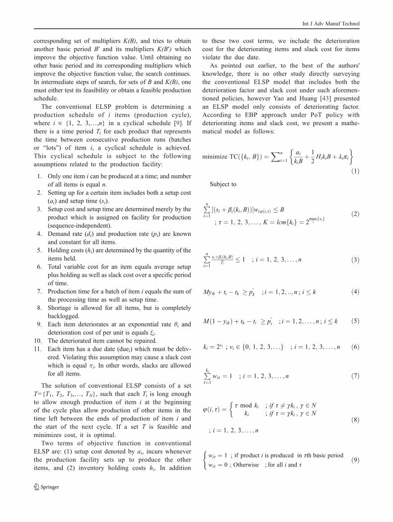
The conventional ELSP problem is determining aproduction schedule of i items (production cycle),where i ∈ {1, 2, 3,…,n} in a cyclical schedule [9]. Ifthere is a time period Ti for each product that representsthe time between consecutive production runs (batchesor “lots”) of item i, a cyclical schedule is achieved.This cyclical schedule is subject to the followingassumptions related to the production facility:

1. Only one item i can be produced at a time; and numberof all items is equal n.

2. Setting up for a certain item includes both a setup cost(ai) and setup time (si).

3. Setup cost and setup time are determined merely by theproduct which is assigned on facility for production(sequence-independent).

4. Demand rate (di) and production rate (pi) are knownand constant for all items.

5. Holding costs (hi) are determined by the quantity of theitems held.

6. Total variable cost for an item equals average setupplus holding as well as slack cost over a specific periodof time.

7. Production time for a batch of item i equals the sum ofthe processing time as well as setup time.

8. Shortage is allowed for all items, but is completelybacklogged.

9. Each item deteriorates at an exponential rate θi anddeterioration cost of per unit is equals ξi.

10. The deteriorated item cannot be repaired.11. Each item has a due date (duei) which must be deliv-

ered. Violating this assumption may cause a slack costwhich is equal πi. In other words, slacks are allowedfor all items.

The solution of conventional ELSP consists of a setT0{T1, T2, T3,…, TN}, such that each Ti is long enoughto allow enough production of item i at the beginningof the cycle plus allow production of other items in thetime left between the ends of production of item i andthe start of the next cycle. If a set T is feasible andminimizes cost, it is optimal.

Two terms of objective function in conventionalELSP are: (1) setup cost denoted by ai, incurs wheneverthe production facility sets up to produce the otheritems, and (2) inventory holding costs hi. In addition

to these two cost terms, we include the deteriorationcost for the deteriorating items and slack cost for itemsviolate the due date.

As pointed out earlier, to the best of the authors'knowledge, there is no other study directly surveyingthe conventional ELSP model that includes both thedeterioration factor and slack cost under such aforemen-tioned policies, however Yao and Huang [43] presentedan ELSP model only consists of deteriorating factor.According to EBP approach under PoT policy withdeteriorating items and slack cost, we present a mathe-matical model as follows:

minimize TC ki; Bf gð Þ ¼Xn

i¼1

aikiB

þ 1

2HikiBþ lipi

� �

ð1ÞSubject to

Pni¼1

si þ biðki;BÞð Þ½ �wi8ði;tÞ � B

; t ¼ 1; 2; 3; . . . ; K ¼ lcmfkig ¼ 2max

ifvig

ð2Þ

Pni¼1

siþbiðki;BÞTi

� 1 ; i ¼ 1; 2; 3; . . . ; n ð3Þ

Myik þ ti � tk � p0k ; i ¼ 1; 2; ::; n ; i � k ð4Þ

Mð1� yikÞ þ tk � ti � p0i ; i ¼ 1; 2; . . . ; n ; i � k ð5Þ

ki ¼ 2vi ; vi 2 0; 1; 2; 3; . . .f g ; i ¼ 1; 2; 3; . . . ; n ð6Þ

Pkit¼1

wit ¼ 1 ; i ¼ 1; 2; 3; . . . ; n ð7Þ

8 ði; tÞ ¼ t mod ki ; if t 6¼ gki ; g 2 Nki ; if t ¼ gki ; g 2 N

�

; i ¼ 1; 2; 3; . . . ; n

ð8Þ

wit ¼ 1 ; if product i is produced in tth basic period

wit ¼ 0 ; Otherwise ; for all i and t

(ð9Þ


li ¼ 1 ; if item i has tardinessli ¼ 0 ; other wise

�; i ¼ 1; 2; 3; . . . ; n

ð10Þ

Hi ¼ di θixi þ hið Þ ; i ¼ 1; 2; 3; . . . ; n ð11Þ

bi ki;Bð Þ ¼ dipi

1þ kiBθi2

� �kiB ; i ¼ 1; 2; 3; . . . ; n ð12Þ

Ci ¼ ti þ p0i ¼ ti þ si þ bi ki;Bð Þð Þ ; i ¼ 1; 2; 3; . . . ; n

ð13Þ

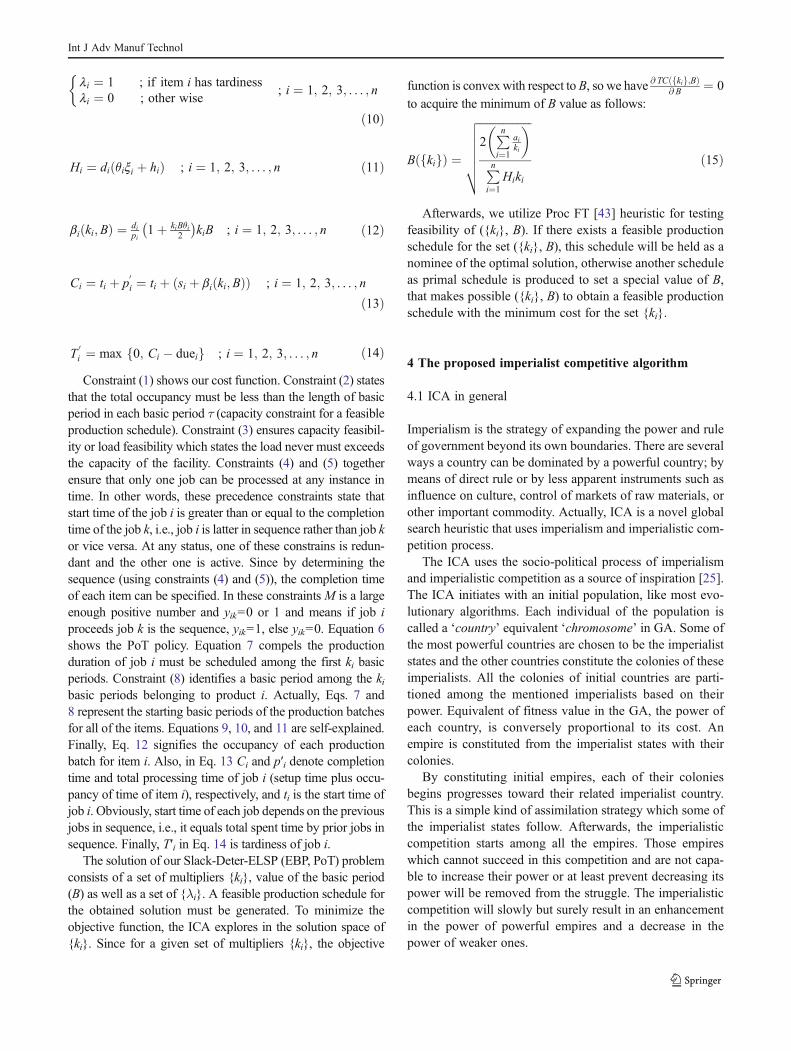
T0i ¼ max 0; Ci � dueif g ; i ¼ 1; 2; 3; . . . ; n ð14ÞConstraint (1) shows our cost function. Constraint (2) states

that the total occupancy must be less than the length of basicperiod in each basic period τ (capacity constraint for a feasibleproduction schedule). Constraint (3) ensures capacity feasibil-ity or load feasibility which states the load never must exceedsthe capacity of the facility. Constraints (4) and (5) togetherensure that only one job can be processed at any instance intime. In other words, these precedence constraints state thatstart time of the job i is greater than or equal to the completiontime of the job k, i.e., job i is latter in sequence rather than job kor vice versa. At any status, one of these constrains is redun-dant and the other one is active. Since by determining thesequence (using constraints (4) and (5)), the completion timeof each item can be specified. In these constraints M is a largeenough positive number and yik00 or 1 and means if job iproceeds job k is the sequence, yik01, else yik00. Equation 6shows the PoT policy. Equation 7 compels the productionduration of job i must be scheduled among the first ki basicperiods. Constraint (8) identifies a basic period among the kibasic periods belonging to product i. Actually, Eqs. 7 and8 represent the starting basic periods of the production batchesfor all of the items. Equations 9, 10, and 11 are self-explained.Finally, Eq. 12 signifies the occupancy of each productionbatch for item i. Also, in Eq. 13 Ci and p′i denote completiontime and total processing time of job i (setup time plus occu-pancy of time of item i), respectively, and ti is the start time ofjob i. Obviously, start time of each job depends on the previousjobs in sequence, i.e., it equals total spent time by prior jobs insequence. Finally, T′i in Eq. 14 is tardiness of job i.

The solution of our Slack-Deter-ELSP (EBP, PoT) problemconsists of a set of multipliers {ki}, value of the basic period(B) as well as a set of {λi}. A feasible production schedule forthe obtained solution must be generated. To minimize theobjective function, the ICA explores in the solution space of{ki}. Since for a given set of multipliers {ki}, the objective

function is convexwith respect to B, so we have @ TCðfkig;BÞ@ B ¼ 0

to acquire the minimum of B value as follows:

BðfkigÞ ¼

ffiffiffiffiffiffiffiffiffiffiffiffiffiffiffiffiffiffiffi2

Pni¼1

aiki

� �

Pni¼1

Hiki

vuuuuut ð15Þ

Afterwards, we utilize Proc FT [43] heuristic for testingfeasibility of ({ki}, B). If there exists a feasible productionschedule for the set ({ki}, B), this schedule will be held as anominee of the optimal solution, otherwise another scheduleas primal schedule is produced to set a special value of B,that makes possible ({ki}, B) to obtain a feasible productionschedule with the minimum cost for the set {ki}.

4 The proposed imperialist competitive algorithm

4.1 ICA in general

Imperialism is the strategy of expanding the power and ruleof government beyond its own boundaries. There are severalways a country can be dominated by a powerful country; bymeans of direct rule or by less apparent instruments such asinfluence on culture, control of markets of raw materials, orother important commodity. Actually, ICA is a novel globalsearch heuristic that uses imperialism and imperialistic com-petition process.

The ICA uses the socio-political process of imperialismand imperialistic competition as a source of inspiration [25].The ICA initiates with an initial population, like most evo-lutionary algorithms. Each individual of the population iscalled a ‘country’ equivalent ‘chromosome’ in GA. Some ofthe most powerful countries are chosen to be the imperialiststates and the other countries constitute the colonies of theseimperialists. All the colonies of initial countries are parti-tioned among the mentioned imperialists based on theirpower. Equivalent of fitness value in the GA, the power ofeach country, is conversely proportional to its cost. Anempire is constituted from the imperialist states with theircolonies.

By constituting initial empires, each of their coloniesbegins progresses toward their related imperialist country.This is a simple kind of assimilation strategy which some ofthe imperialist states follow. Afterwards, the imperialisticcompetition starts among all the empires. Those empireswhich cannot succeed in this competition and are not capa-ble to increase their power or at least prevent decreasing itspower will be removed from the struggle. The imperialisticcompetition will slowly but surely result in an enhancementin the power of powerful empires and a decrease in thepower of weaker ones.


The total power of an empire depends on both the powerof the imperialist country and the power of its colonies. Thisfact is modeled by defining the total power of an empire asthe power of imperialist country plus a percentage of meanpower of its colonies [25].

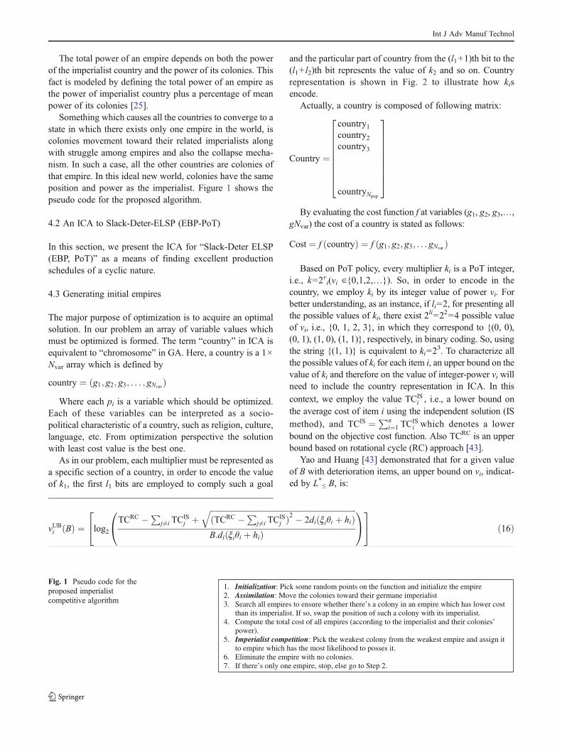
Something which causes all the countries to converge to astate in which there exists only one empire in the world, iscolonies movement toward their related imperialists alongwith struggle among empires and also the collapse mecha-nism. In such a case, all the other countries are colonies ofthat empire. In this ideal new world, colonies have the sameposition and power as the imperialist. Figure 1 shows thepseudo code for the proposed algorithm.

4.2 An ICA to Slack-Deter-ELSP (EBP-PoT)

In this section, we present the ICA for “Slack-Deter ELSP(EBP, PoT)” as a means of finding excellent productionschedules of a cyclic nature.

4.3 Generating initial empires

The major purpose of optimization is to acquire an optimalsolution. In our problem an array of variable values whichmust be optimized is formed. The term “country” in ICA isequivalent to “chromosome” in GA. Here, a country is a 1×Nvar array which is defined by

country ¼ g1; g2; g3; . . . ; gNvarð ÞWhere each pi is a variable which should be optimized.

Each of these variables can be interpreted as a socio-political characteristic of a country, such as religion, culture,language, etc. From optimization perspective the solutionwith least cost value is the best one.

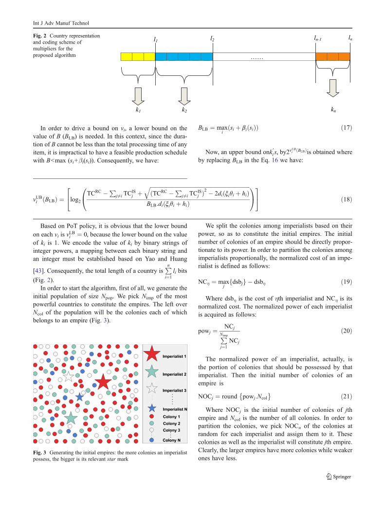
As in our problem, each multiplier must be represented asa specific section of a country, in order to encode the valueof k1, the first l1 bits are employed to comply such a goal

and the particular part of country from the (l1+1)th bit to the(l1+ l2)th bit represents the value of k2 and so on. Countryrepresentation is shown in Fig. 2 to illustrate how kisencode.

Actually, a country is composed of following matrix:

Country ¼

country1country2country3

countryNpop

2666666664

3777777775

By evaluating the cost function f at variables (g1, g2, g3,…,gNvar) the cost of a country is stated as follows:

Cost ¼ f countryð Þ ¼ f g1; g2; g3; . . . gNvarð Þ

Based on PoT policy, every multiplier ki is a PoT integer,i.e., k02vi(vi ∈{0,1,2,…}). So, in order to encode in thecountry, we employ ki by its integer value of power vi. Forbetter understanding, as an instance, if li02, for presenting allthe possible values of ki, there exist 2

li02204 possible valueof vi, i.e., {0, 1, 2, 3}, in which they correspond to {(0, 0),(0, 1), (1, 0), (1, 1)}, respectively, in binary coding. So, usingthe string {(1, 1)} is equivalent to ki02

3. To characterize allthe possible values of ki for each item i, an upper bound on thevalue of ki and therefore on the value of integer-power vi willneed to include the country representation in ICA. In this

context, we employ the value TCISi , i.e., a lower bound on

the average cost of item i using the independent solution (IS

method), and TCIS ¼ Pni¼1 TC

ISi which denotes a lower

bound on the objective cost function. Also TCRC is an upperbound based on rotational cycle (RC) approach [43].

Yao and Huang [43] demonstrated that for a given valueof B with deterioration items, an upper bound on vi, indicat-ed by L*≤ B, is:

vUBi ðBÞ ¼ log2TCRC �P

j6¼i TCISj þ

ffiffiffiffiffiffiffiffiffiffiffiffiffiffiffiffiffiffiffiffiffiffiffiffiffiffiffiffiffiffiffiffiffiffiffiffiffiffiffiffiffiffiffiffiffiffiffiffiffiffiffiffiffiffiffiffiffiffiffiffiffiffiffiffiffiffiffiffiffiffiffiffiffiffiðTCRC �P

j6¼i TCISj Þ

2 � 2di xiθi þ hið ÞqB:di xiθi þ hið Þ

0@

1A

24

35 ð16Þ

1. Initialization: Pick some random points on the function and initialize the empire 2. Assimilation: Move the colonies toward their germane imperialist 3. Search all empires to ensure whether there’s a colony in an empire which has lower cost

than its imperialist. If so, swap the position of such a colony with its imperialist. 4. Compute the total cost of all empires (according to the imperialist and their colonies’

power). 5. Imperialist competition: Pick the weakest colony from the weakest empire and assign it

to empire which has the most likelihood to posses it. 6. Eliminate the empire with no colonies. 7. If there’s only one empire, stop, else go to Step 2.

Fig. 1 Pseudo code for theproposed imperialistcompetitive algorithm


In order to drive a bound on vi, a lower bound on thevalue of B (BLB) is needed. In this context, since the dura-tion of B cannot be less than the total processing time of anyitem, it is impractical to have a feasible production schedulewith B<max (si+βi(si)). Consequently, we have:

BLB ¼ maxiðsi þ biðsiÞÞ ð17Þ

Now, an upper bound onk0i s, by2

vUBi ðBLBÞis obtained whereby replacing BLB in the Eq. 16 we have:

vUBi BLBð Þ ¼ log2TCRC �P

j 6¼i TCISj þ

ffiffiffiffiffiffiffiffiffiffiffiffiffiffiffiffiffiffiffiffiffiffiffiffiffiffiffiffiffiffiffiffiffiffiffiffiffiffiffiffiffiffiffiffiffiffiffiffiffiffiffiffiffiffiffiffiffiffiffiffiffiffiffiffiffiffiffiffiffiffiffiffiffiffiðTCRC �P

j6¼i TCISj Þ

2 � 2di xiθi þ hið ÞqBLB:di xiθi þ hið Þ

0@

1A

24

35 ð18Þ

Based on PoT policy, it is obvious that the lower boundon each vi is vLBi ¼ 0, because the lower bound on the valueof ki is 1. We encode the value of ki by binary strings ofinteger powers, a mapping between each binary string andan integer must be established based on Yao and Huang

[43]. Consequently, the total length of a country isPni¼1

li bits

(Fig. 2).In order to start the algorithm, first of all, we generate the

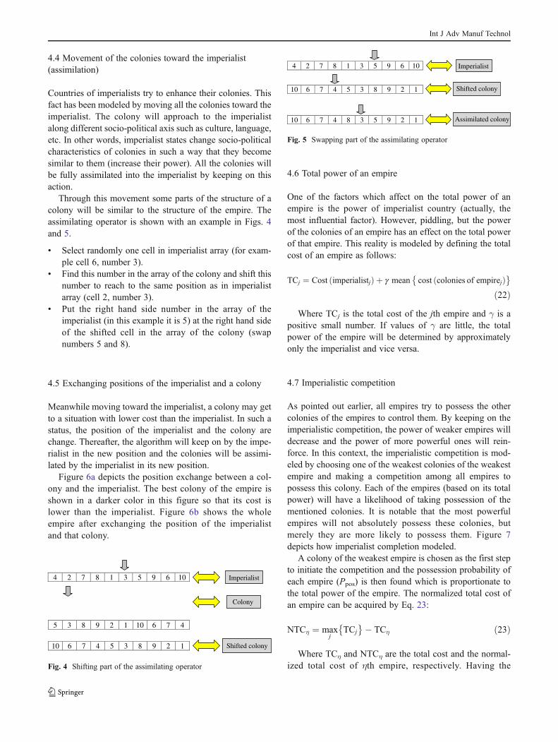
initial population of size Npop. We pick Nimp of the mostpowerful countries to constitute the empires. The left overNcol of the population will be the colonies each of whichbelongs to an empire (Fig. 3).

We split the colonies among imperialists based on theirpower, so as to constitute the initial empires. The initialnumber of colonies of an empire should be directly propor-tionate to its power. In order to partition the colonies amongimperialists proportionally, the normalized cost of an impe-rialist is defined as follows:

NCη ¼ maxjfdsbjg � dsbη ð19Þ

Where dsbη is the cost of ηth imperialist and NCη is itsnormalized cost. The normalized power of each imperialistis acquired as follows:

powj ¼ NCj

PNimp

j¼1NCj

ð20Þ

The normalized power of an imperialist, actually, isthe portion of colonies that should be possessed by thatimperialist. Then the initial number of colonies of anempire is

NOCj ¼ round powj:Ncol

ð21ÞWhere NOCj is the initial number of colonies of jth

empire and Ncol is the number of all colonies. In order topartition the colonies, we pick NOCn of the colonies atrandom for each imperialist and assign them to it. Thesecolonies as well as the imperialist will constitute jth empire.Clearly, the larger empires have more colonies while weakerones have less.

……

k2 k1

l1 l2

kn

ln-1 lnFig. 2 Country representationand coding scheme ofmultipliers for theproposed algorithm

Fig. 3 Generating the initial empires: the more colonies an imperialistpossess, the bigger is its relevant star mark


4.4 Movement of the colonies toward the imperialist(assimilation)

Countries of imperialists try to enhance their colonies. Thisfact has been modeled by moving all the colonies toward theimperialist. The colony will approach to the imperialistalong different socio-political axis such as culture, language,etc. In other words, imperialist states change socio-politicalcharacteristics of colonies in such a way that they becomesimilar to them (increase their power). All the colonies willbe fully assimilated into the imperialist by keeping on thisaction.

Through this movement some parts of the structure of acolony will be similar to the structure of the empire. Theassimilating operator is shown with an example in Figs. 4and 5.

& Select randomly one cell in imperialist array (for exam-ple cell 6, number 3).

& Find this number in the array of the colony and shift thisnumber to reach to the same position as in imperialistarray (cell 2, number 3).

& Put the right hand side number in the array of theimperialist (in this example it is 5) at the right hand sideof the shifted cell in the array of the colony (swapnumbers 5 and 8).

4.5 Exchanging positions of the imperialist and a colony

Meanwhile moving toward the imperialist, a colony may getto a situation with lower cost than the imperialist. In such astatus, the position of the imperialist and the colony arechange. Thereafter, the algorithm will keep on by the impe-rialist in the new position and the colonies will be assimi-lated by the imperialist in its new position.

Figure 6a depicts the position exchange between a col-ony and the imperialist. The best colony of the empire isshown in a darker color in this figure so that its cost islower than the imperialist. Figure 6b shows the wholeempire after exchanging the position of the imperialistand that colony.

4.6 Total power of an empire

One of the factors which affect on the total power of anempire is the power of imperialist country (actually, themost influential factor). However, piddling, but the powerof the colonies of an empire has an effect on the total powerof that empire. This reality is modeled by defining the totalcost of an empire as follows:

TCj ¼ Cost ðimperialistjÞ þ g mean cost ðcolonies of empirejÞ

ð22ÞWhere TCj is the total cost of the jth empire and γ is a

positive small number. If values of γ are little, the totalpower of the empire will be determined by approximatelyonly the imperialist and vice versa.

4.7 Imperialistic competition

As pointed out earlier, all empires try to possess the othercolonies of the empires to control them. By keeping on theimperialistic competition, the power of weaker empires willdecrease and the power of more powerful ones will rein-force. In this context, the imperialistic competition is mod-eled by choosing one of the weakest colonies of the weakestempire and making a competition among all empires topossess this colony. Each of the empires (based on its totalpower) will have a likelihood of taking possession of thementioned colonies. It is notable that the most powerfulempires will not absolutely possess these colonies, butmerely they are more likely to possess them. Figure 7depicts how imperialist completion modeled.

A colony of the weakest empire is chosen as the first stepto initiate the competition and the possession probability ofeach empire (Ppos) is then found which is proportionate tothe total power of the empire. The normalized total cost ofan empire can be acquired by Eq. 23:

NTCη ¼ maxj

TCj

� TCη ð23Þ

Where TCη and NTCη are the total cost and the normal-ized total cost of ηth empire, respectively. Having the

4 2 7 8 1 3 5 9 6 10

Colony

Imperialist

5 3 8 9 2 1 10 6 7 4

10 6 7 4 5 3 8 9 2 1 Shifted colony

Fig. 4 Shifting part of the assimilating operator

4 2 7 8 1 3 5 9 6 10

10 6 7 4 5 3 8 9 2 1

10 6 7 4 8 3 5 9 2 1

Imperialist

Shifted colony

Assimilated colony

Fig. 5 Swapping part of the assimilating operator


normalized total cost, the possession probability of ηthempire will be known as follows:

Pposη ¼NTCη

PNimp

j¼1NTCj

ð24Þ

Choosing an empire is analogous to the roulette wheelprocess which is used in selecting parents in GA, but sincein this method calculation of the cumulative distributionfunction is not needed, i.e., the selection is based on onlythe values of probabilities of selection. Consequently, thismethod is much faster than the conventional roulette wheel.Based on aforementioned explanations, the process ofchoosing the empires can substitute the roulette wheel inGA and therefore causes an increase in its computationalspeed.

In order to partition the mentioned colonies amongempires based on the possession probability of them, vectorP is formed as follows:

P ¼ ½ppos1 ; ppos2 ; :::; pposNimp�

Afterward, we create a vector R with the same size as Pwhose elements are uniformly distributed random numbersas follows:

R ¼ r1; r2; :::; rNimp

� �; r1; r2; . . . ; rNimp 2 Uð0; 1Þ

Vector E can be acquired by subtracting R from P:

E ¼ P � R ¼ E1;E2; . . .ENimp

� �

¼ ppos1 � r1; ppos2 � r2; . . . ; pposNimp� rNimp

h i

Fig. 6 a Exchanging thepositions of a colony and theimperialist; b the entire empireafter position exchange

Fig. 7 The more powerfulan empire is, the more likely itwill possess the weakest colonyof the weakest empire(Imperialistic competition)


Referring to vector E, the mentioned colony (colonies)will hand to an empire whose relevant index in E ismaximum.

4.8 Elimination of the powerless empires

Those empires which are powerless will collapse in theimperialistic competition and their colonies will be parti-tioned among other empires. Different criteria can be intro-duced so as to consider a powerless empire in collapsemechanism modeling, such as “time limitation” or “maxi-mum number of iterations”. When an empire loses all of itscolonies, in fact, this empire is collapsed and consequently,will be eliminated. This is the mechanism which we use inour problem.

4.9 Convergence and stop criterion

By keeping on the algorithm and spending the time, all ofthe empires will collapse except the most powerful one andall the colonies will be subjected to this empire. In such anideal new world, all the colonies will have the same posi-tions and same costs and they will be controlled by animperialist with the same position and cost as themselves.In such a world, there is no difference not only amongcolonies, but also between colonies and imperialist.

5 GA for Slack-Deter-ELSP (EBP, PoT)

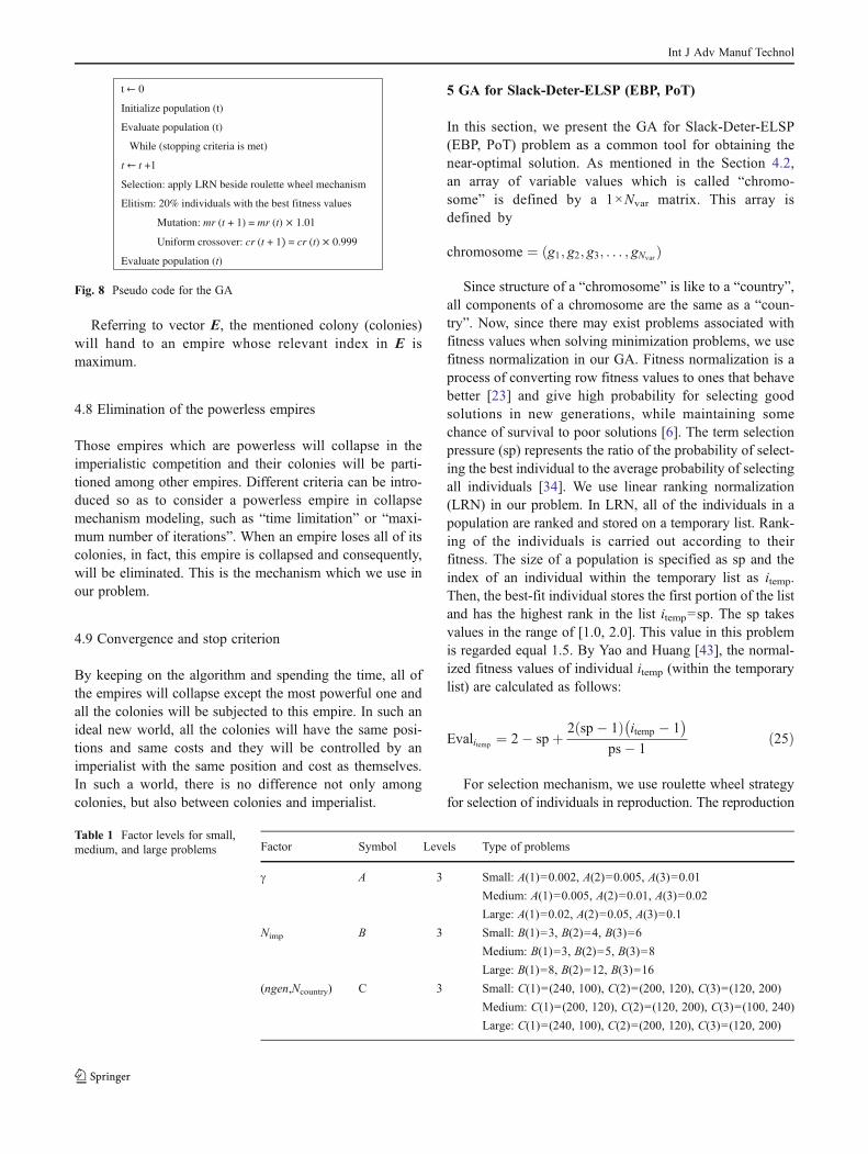
In this section, we present the GA for Slack-Deter-ELSP(EBP, PoT) problem as a common tool for obtaining thenear-optimal solution. As mentioned in the Section 4.2,an array of variable values which is called “chromo-some” is defined by a 1×Nvar matrix. This array isdefined by

chromosome ¼ g1; g2; g3; . . . ; gNvarð Þ

Since structure of a “chromosome” is like to a “country”,all components of a chromosome are the same as a “coun-try”. Now, since there may exist problems associated withfitness values when solving minimization problems, we usefitness normalization in our GA. Fitness normalization is aprocess of converting row fitness values to ones that behavebetter [23] and give high probability for selecting goodsolutions in new generations, while maintaining somechance of survival to poor solutions [6]. The term selectionpressure (sp) represents the ratio of the probability of select-ing the best individual to the average probability of selectingall individuals [34]. We use linear ranking normalization(LRN) in our problem. In LRN, all of the individuals in apopulation are ranked and stored on a temporary list. Rank-ing of the individuals is carried out according to theirfitness. The size of a population is specified as sp and theindex of an individual within the temporary list as itemp.Then, the best-fit individual stores the first portion of the listand has the highest rank in the list itemp0sp. The sp takesvalues in the range of [1.0, 2.0]. This value in this problemis regarded equal 1.5. By Yao and Huang [43], the normal-ized fitness values of individual itemp (within the temporarylist) are calculated as follows:

Evalitemp ¼ 2� spþ 2 sp� 1ð Þ itemp � 1� �

ps� 1ð25Þ

For selection mechanism, we use roulette wheel strategyfor selection of individuals in reproduction. The reproduction

t 0

Initialize population (t)

Evaluate population (t)

While (stopping criteria is met)

t t +1

Selection: apply LRN beside roulette wheel mechanism

Elitism: 20% individuals with the best fitness values

Mutation: mr (t + 1) = mr (t) 1.01

Uniform crossover: cr (t + 1 = cr (t) 0.999

Evaluate population (t)

Fig. 8 Pseudo code for the GA

Table 1 Factor levels for small,medium, and large problems Factor Symbol Levels Type of problems

+ A 3 Small: A(1)00.002, A(2)00.005, A(3)00.01

Medium: A(1)00.005, A(2)00.01, A(3)00.02

Large: A(1)00.02, A(2)00.05, A(3)00.1

Nimp B 3 Small: B(1)03, B(2)04, B(3)06

Medium: B(1)03, B(2)05, B(3)08

Large: B(1)08, B(2)012, B(3)016

(ngen,Ncountry) C 3 Small: C(1)0(240, 100), C(2)0(200, 120), C(3)0(120, 200)

Medium: C(1)0(200, 120), C(2)0(120, 200), C(3)0(100, 240)

Large: C(1)0(240, 100), C(2)0(200, 120), C(3)0(120, 200)


probability of each individual is proportional to its normalizedfitness as expressed in Eq. 26 as follows:

Pitemp ¼EvalitempPps

itemp¼1Evalitemp

ð26Þ

Uniform crossover strategy is applied to this problembecause it is assumed to reduce the bias associated withthe length of the binary representation used and the partic-ular coding for a given parameter set [34]. The mutationoperator randomly selects ones among the genes of allindividuals in the population with a fixed mutation rate(mr). The population size is recommended to be set asPS010n (n05, 10 and 15). The crossover rate (cr) and themutation rate vary linearly during the evolutionary process.We set the cr at a higher level (0.9) in the start of theevolution while the mr is lower (0.05), in order that ourGA can take advantage of the characteristics of the individ-ual. Through the evolutionary process, the crossover rate foreach generation decreases by 0.001 and the mutation rateincreases by 0.01 after 100 generations. The variation of crand mr stop as they reach a specified level, i.e., cr00.2 andmr00.2. Using such policy our GA is capable still to explorenew area in the search space and increase the populationdiversity, since at the end of evolution the individuals

become similar to each other (because of cr decreases whilemr increases). In our paper, one of the “time limitation” or“50 nonimprovement iterations” is determined as stoppingcriteria. Our GA procedure is shown in Fig. 8 as follows:

6 Generation of feasible production schedule

At first, we need to obtain a production schedule of eachitem by assigning the production lots of all the items. Fur-thermore, we have to determine the set of variables {wit}.

In the literature, Yao et al. [42] showed being NP-completeness of the problem of generating a feasible pro-duction schedule for a given set of ({ki}, B) for the conven-tional ELSP (EBP, PoT) model. Showing the complexity ofNP-completeness of the Deter-ELSP (EBP, PoT) model isvery easy. So being NP-completeness of Slack-Deter-ELSP(EBP-PoT) is evident. For obtaining a feasibility testingprocedure, we use Proc FT [43] with some changes. Sup-pose G signify a candidate schedule and L(G) be the max-imal load secured by G. Presume that a set of multipliers{ki} and B is given. The corresponding occupancy times βi(ki, B)} evidently will be determined. Use a random produc-tion schedule to acquire an initial schedule of production G,and calculate L(G). Regard L* as the best load secured up to

Table 2 Taguchi orthogonalarray design No + Nimp (ngen,

Ncountry)

1 1 1 1

2 1 2 2

3 1 3 3

4 2 1 2

5 2 2 3

6 2 3 1

7 3 1 3

8 3 2 1

9 3 3 2

Table 3 Problems data sets

Input variables Distribution

Demand rate (di) õ DU[2,000, 60,000]

Produce rate (pi) õ DU[5,000, 125,000]

Holding cost (hi) õ DU[5, 120]

Setup cost (ai) õ DU[60, 600]

Setup time (si) õ DU[5, 15]

Deterioration cost (ξi) õ DU[10, 110]

Deterioration factor (θi) õ U[0.3, 3]

Due date (duei) õ DU[30, 85]

Slack cost (πi) õ DU[80, 500]

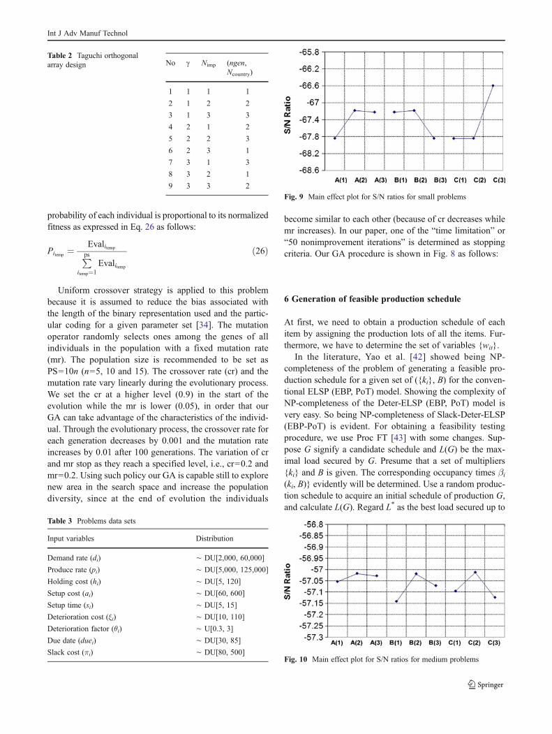
Fig. 9 Main effect plot for S/N ratios for small problems

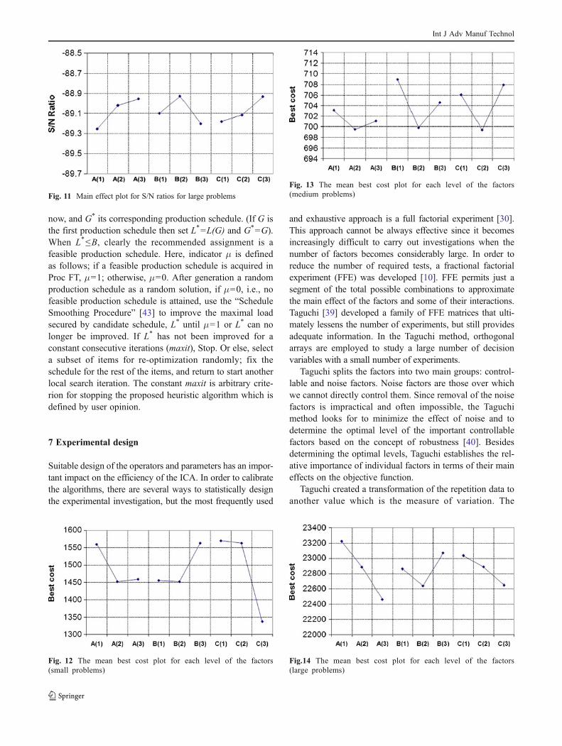
Fig. 10 Main effect plot for S/N ratios for medium problems


now, and G* its corresponding production schedule. (If G isthe first production schedule then set L*0L(G) and G*0G).When L*≤B, clearly the recommended assignment is afeasible production schedule. Here, indicator μ is definedas follows; if a feasible production schedule is acquired inProc FT, μ01; otherwise, μ00. After generation a randomproduction schedule as a random solution, if μ00, i.e., nofeasible production schedule is attained, use the “ScheduleSmoothing Procedure” [43] to improve the maximal loadsecured by candidate schedule, L* until μ01 or L* can nolonger be improved. If L* has not been improved for aconstant consecutive iterations (maxit), Stop. Or else, selecta subset of items for re-optimization randomly; fix theschedule for the rest of the items, and return to start anotherlocal search iteration. The constant maxit is arbitrary crite-rion for stopping the proposed heuristic algorithm which isdefined by user opinion.

7 Experimental design

Suitable design of the operators and parameters has an impor-tant impact on the efficiency of the ICA. In order to calibratethe algorithms, there are several ways to statistically designthe experimental investigation, but the most frequently used

and exhaustive approach is a full factorial experiment [30].This approach cannot be always effective since it becomesincreasingly difficult to carry out investigations when thenumber of factors becomes considerably large. In order toreduce the number of required tests, a fractional factorialexperiment (FFE) was developed [10]. FFE permits just asegment of the total possible combinations to approximatethe main effect of the factors and some of their interactions.Taguchi [39] developed a family of FFE matrices that ulti-mately lessens the number of experiments, but still providesadequate information. In the Taguchi method, orthogonalarrays are employed to study a large number of decisionvariables with a small number of experiments.

Taguchi splits the factors into two main groups: control-lable and noise factors. Noise factors are those over whichwe cannot directly control them. Since removal of the noisefactors is impractical and often impossible, the Taguchimethod looks for to minimize the effect of noise and todetermine the optimal level of the important controllablefactors based on the concept of robustness [40]. Besidesdetermining the optimal levels, Taguchi establishes the rel-ative importance of individual factors in terms of their maineffects on the objective function.

Taguchi created a transformation of the repetition data toanother value which is the measure of variation. The

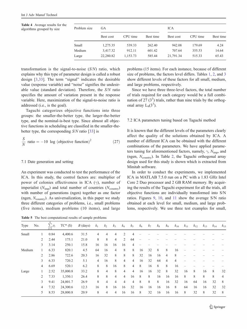
Fig. 11 Main effect plot for S/N ratios for large problems

Fig. 12 The mean best cost plot for each level of the factors(small problems)

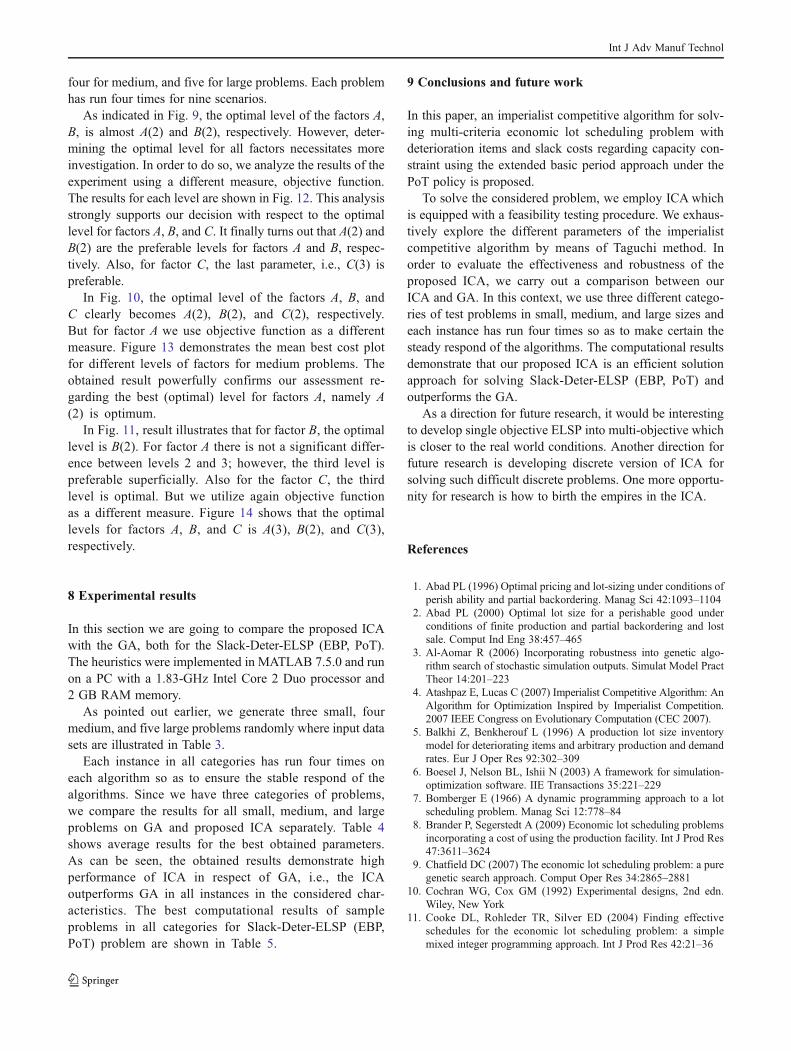
Fig. 13 The mean best cost plot for each level of the factors(medium problems)

Fig.14 The mean best cost plot for each level of the factors(large problems)


transformation is the signal-to-noise (S/N) ratio, whichexplains why this type of parameter design is called a robustdesign [3,33]. The term “signal” indicates the desirablevalue (response variable) and “noise” signifies the undesir-able value (standard deviation). Therefore, the S/N ratiospecifies the amount of variation present in the responsevariable. Here, maximization of the signal-to-noise ratio isaddressed (i.e., is the goal).

Taguchi categorizes objective functions into threegroups: the smaller-the-better type, the larger-the-bettertype, and the nominal-is-best type. Since almost all objec-tive functions in scheduling are classified in the smaller-the-better type, the corresponding S/N ratio [33] is

S

Nratio ¼ �10 log objective functionð Þ2 ð27Þ

7.1 Date generation and setting

An experiment was conducted to test the performance of theICA. In this study, the control factors are: multiplier ofpower of colonies effectiveness in ICA (γ), number ofimperialist (Nimp) and total number of countries (Ncountry)with number of generations (ngen) together as one factor(ngen, Ncountry). As universalization, in this paper we studythree different categories of problems, i.e., small problems(five items), medium problems (10 items), and large

problems (15 items). For each instance, because of differentsize of problems, the factors level differs. Tables 1, 2, and 3show different levels of these factors for all small, medium,and large problems, respectively.

Since we have three three-level factors, the total numberof trials required for each category would be a full combi-nation of 27 (33) trials, rather than nine trials by the orthog-onal array L9(3

3).

7.2 ICA parameters tuning based on Taguchi method

It is known that the different levels of the parameters clearlyaffect the quality of the solutions obtained by ICA. Anumber of different ICA can be obtained with the differentcombinations of the parameters. We have applied parame-ters tuning for aforementioned factors, namely, γ, Nimp, and(ngen, Ncountry). In Table 2, the Taguchi orthogonal arraydesign used for this study is shown which is extracted fromMinitab software.

In order to conduct the experiments, we implementedICA in MATLAB 7.5.0 run on a PC with a 1.83 GHz IntelCore 2 Duo processor and 2 GB RAM memory. By acquir-ing the results of the Taguchi experiment for all the trials, allobjective functions are individually transformed into S/Nratios. Figures 9, 10, and 11 show the average S/N ratioobtained at each level for small, medium, and large prob-lems, respectively. We use three test examples for small,

Table 4 Average results for thealgorithms grouped by size Problem size GA ICA

Best cost CPU time Best time Best cost CPU time Best time

Small 1,275.35 539.33 262.40 942.08 179.69 4.24

Medium 3,417.32 912.11 601.42 707.64 355.53 14.64

Large 22,280.82 1,153.73 585.44 21,791.34 515.33 65.43

Table 5 The best computational results of sample problems

Type No.Pni¼1

ρi TC* ($) B (days) k1 k2 k3 k4 k5 k6 k7 k8 k9 k10 k11 k12 k13 k14 k15

Small 1 0.84 4,400.6 31.5 4 4 4 2 4 – – – – – – – – – –

2 2.44 175.1 21.0 8 8 4 2 64 – – – – – – – – – –

3 3.14 250.1 15.8 16 16 16 16 4 – – – – – – – – – –

Medium 1 6.33 820.1 4.5 64 16 4 8 8 16 32 8 8 16 – – – – –

2 2.86 722.6 20.3 16 32 8 8 8 32 16 16 4 8 – – – – –

3 6.33 720.2 5.1 4 16 8 4 4 16 32 64 4 4 – – – – –

4 6.69 520.1 6.2 8 8 16 8 4 8 16 8 8 16 – – – – –

Large 1 2.52 35,000.8 33.2 8 4 8 4 4 16 16 32 8 32 16 8 16 8 32

2 7.33 1,350.1 26.4 8 8 4 4 16 8 8 16 16 16 8 8 8 8 4

3 9.41 24,001.7 26.9 8 4 4 4 4 8 8 8 16 32 16 64 16 32 8

4 7.32 24,300.6 12.3 16 8 16 16 32 16 16 16 16 8 64 16 16 32 32

5 8.53 28,000.8 20.9 8 4 4 16 16 8 32 16 16 16 8 32 8 32 8


four for medium, and five for large problems. Each problemhas run four times for nine scenarios.

As indicated in Fig. 9, the optimal level of the factors A,B, is almost A(2) and B(2), respectively. However, deter-mining the optimal level for all factors necessitates moreinvestigation. In order to do so, we analyze the results of theexperiment using a different measure, objective function.The results for each level are shown in Fig. 12. This analysisstrongly supports our decision with respect to the optimallevel for factors A, B, and C. It finally turns out that A(2) andB(2) are the preferable levels for factors A and B, respec-tively. Also, for factor C, the last parameter, i.e., C(3) ispreferable.

In Fig. 10, the optimal level of the factors A, B, andC clearly becomes A(2), B(2), and C(2), respectively.But for factor A we use objective function as a differentmeasure. Figure 13 demonstrates the mean best cost plotfor different levels of factors for medium problems. Theobtained result powerfully confirms our assessment re-garding the best (optimal) level for factors A, namely A(2) is optimum.

In Fig. 11, result illustrates that for factor B, the optimallevel is B(2). For factor A there is not a significant differ-ence between levels 2 and 3; however, the third level ispreferable superficially. Also for the factor C, the thirdlevel is optimal. But we utilize again objective functionas a different measure. Figure 14 shows that the optimallevels for factors A, B, and C is A(3), B(2), and C(3),respectively.

8 Experimental results

In this section we are going to compare the proposed ICAwith the GA, both for the Slack-Deter-ELSP (EBP, PoT).The heuristics were implemented in MATLAB 7.5.0 and runon a PC with a 1.83-GHz Intel Core 2 Duo processor and2 GB RAM memory.

As pointed out earlier, we generate three small, fourmedium, and five large problems randomly where input datasets are illustrated in Table 3.

Each instance in all categories has run four times oneach algorithm so as to ensure the stable respond of thealgorithms. Since we have three categories of problems,we compare the results for all small, medium, and largeproblems on GA and proposed ICA separately. Table 4shows average results for the best obtained parameters.As can be seen, the obtained results demonstrate highperformance of ICA in respect of GA, i.e., the ICAoutperforms GA in all instances in the considered char-acteristics. The best computational results of sampleproblems in all categories for Slack-Deter-ELSP (EBP,PoT) problem are shown in Table 5.

9 Conclusions and future work

In this paper, an imperialist competitive algorithm for solv-ing multi-criteria economic lot scheduling problem withdeterioration items and slack costs regarding capacity con-straint using the extended basic period approach under thePoT policy is proposed.

To solve the considered problem, we employ ICA whichis equipped with a feasibility testing procedure. We exhaus-tively explore the different parameters of the imperialistcompetitive algorithm by means of Taguchi method. Inorder to evaluate the effectiveness and robustness of theproposed ICA, we carry out a comparison between ourICA and GA. In this context, we use three different catego-ries of test problems in small, medium, and large sizes andeach instance has run four times so as to make certain thesteady respond of the algorithms. The computational resultsdemonstrate that our proposed ICA is an efficient solutionapproach for solving Slack-Deter-ELSP (EBP, PoT) andoutperforms the GA.

As a direction for future research, it would be interestingto develop single objective ELSP into multi-objective whichis closer to the real world conditions. Another direction forfuture research is developing discrete version of ICA forsolving such difficult discrete problems. One more opportu-nity for research is how to birth the empires in the ICA.

References

1. Abad PL (1996) Optimal pricing and lot-sizing under conditions ofperish ability and partial backordering. Manag Sci 42:1093–1104

2. Abad PL (2000) Optimal lot size for a perishable good underconditions of finite production and partial backordering and lostsale. Comput Ind Eng 38:457–465

3. Al-Aomar R (2006) Incorporating robustness into genetic algo-rithm search of stochastic simulation outputs. Simulat Model PractTheor 14:201–223

4. Atashpaz E, Lucas C (2007) Imperialist Competitive Algorithm: AnAlgorithm for Optimization Inspired by Imperialist Competition.2007 IEEE Congress on Evolutionary Computation (CEC 2007).

5. Balkhi Z, Benkherouf L (1996) A production lot size inventorymodel for deteriorating items and arbitrary production and demandrates. Eur J Oper Res 92:302–309

6. Boesel J, Nelson BL, Ishii N (2003) A framework for simulation-optimization software. IIE Transactions 35:221–229

7. Bomberger E (1966) A dynamic programming approach to a lotscheduling problem. Manag Sci 12:778–84

8. Brander P, Segerstedt A (2009) Economic lot scheduling problemsincorporating a cost of using the production facility. Int J Prod Res47:3611–3624

9. Chatfield DC (2007) The economic lot scheduling problem: a puregenetic search approach. Comput Oper Res 34:2865–2881

10. Cochran WG, Cox GM (1992) Experimental designs, 2nd edn.Wiley, New York

11. Cooke DL, Rohleder TR, Silver ED (2004) Finding effectiveschedules for the economic lot scheduling problem: a simplemixed integer programming approach. Int J Prod Res 42:21–36


12. Dobson G (1987) The ELSP: achieving feasibility using time-varying lot sizes. Oper Res 35(5):764–71

13. Eilon S (1958) Economic batch size determination for multiprod-uct scheduling. Oper Res Q 10:217–277

14. Elmaghraby SE (1978) The economic lot scheduling problem(ELSP): review and extension. Manag Sci 24:587–597

15. Elsayed EA, Teresi C (1983) Analysis of inventory system withdeteriorating items. Int J Prod Res 21:449–460

16. Federgruen A, Zheng YS (1993) Optimal power-of-two replenish-ment strategies in capacitated general production distribution net-works. Manag Sci 39:710–727

17. Gallego G, Joneja D (1994) Economic lot scheduling problem withraw material considerations. Oper Res 42(1):92–101

18. Ghare PM, Schrader GF (1963) A model for an exponentiallydecaying inventory. J Ind Eng 14:238–243

19. Goyal SK (1975) Scheduling a multi-product single machine sys-tem—a new approach. Int J Prod Res 13:487–93

20. Heng KJ, Labban J, Linn RJ (1991) An order-level lot-size inven-tory model for deteriorating items with finite replenishment rate.Comput Ind Eng 20:187–197

21. Heydari M, Torabi SA (2008) The economic lot scheduling prob-lem in flow lines with sequence-dependent setups. World Acade-my of Science Eng Tech 47:2008

22. Hsu WL (1983) On the general feasibility of scheduling lot sizes ofseveral products on one machine. Manag Sci 29:93–105

23. Hunter A (1998) Crossing over genetic algorithms: the Sugalgeneralized GA. Journal of Heuristics 4:179–192

24. Jackson PL, Maxwell WL, Muckstadt JA (1985) The joint replen-ishment problem with a power-of-two restriction. IIE Trans 17:25–32

25. Khabbazi A, Atashpaz E, Lucas C (2009) Imperialist competitivealgorithm for minimum bit error rate beamforming. Int J Bio-Inspired Comput 1:125–133

26. Lopez MA, Kingsman BG (1991) The economic lot schedul-ing problem: theory and practice. Int J Prod Econ 23:147–164

27. Luss H, Rosenwein MB (1990) A lot-sizing model for just-in-timemanufacturing. J Oper Res Soc 41(3):201–209

28. Maxwell WL (1964) The scheduling of economic lot sizes. NavRes Logist Q 11:89–124

29. Misra RB (1975) Optimal production lot size model for a systemwith deteriorating items. Int J Prod Res 13:495–505

30. Montgomery DC (2000) Design and analysis of experiments, 5thedn. Wiley, New York

31. Moon IK, Cha BC, Bae HC (2006) Hybrid genetic algorithm forgroup technology economic lot scheduling problem. Int J Prod Res44:4551–4568

32. Nahmias S (1978) Perishable inventory theory: a review. Oper Res30:680–708

33. Phadke MS (1989) Quality engineering using robust design.Prentice-Hall, Engelwood Cliffs

34. Pohlheim H (2001) Evolutionary algorithms: principles, methods,and algorithms [online]. Available from: http://www.geatbx.com/index.html, [accessed on 6 May 2004].

35. Raafat F (1991) Survey of literature on continuously deterioratinginventory models. J Oper Res Soc 42:27–37

36. Roundy R (1984) Rounding off to powers of two in continuousrelaxations of capacitated lot sizing problems. Manag Sci35:1433–1442

37. Soman CA, Van Donk DP, Gaalman G (2003) Combined make-to-order and make-to-stock in a food production system. To appear inInternational Journal of Production Economics, http://dx.doi.org/10.1016/S0925-5273(02)00376-6.

38. Soman CA, Van Donk DP, Gaalman G (2004) A basic periodapproach to the economic lot scheduling problem with shelf lifeconsiderations. Int J Prod Res 42:1677–1689

39. Taguchi G (1986) Introduction to quality engineering. Asian Pro-ductivity, White Plains

40. Tsai JT, Ho WH, Liu TK, Chou JH (2007) Improved immunealgorithm for global numerical optimisation and job-shop sched-uling problems. Appl Math Comput 194:406–424

41. Yao MJ, Elmaghraby SE (2001) The economic lot schedulingproblem under power-of-two policy. Comput Math Appl (CMWA)41:1379–1393

42. Yao MJ, Elmaghraby SE, Chen IC (2003) On the feasibility testingof the economic lot scheduling problem using the extended basicperiod approach. J Chin Inst Ind Eng 20:435–448

43. Yao MJ, Huang JX (2005) Solving the economic lot schedulingproblem with deteriorating items using genetic algorithms. J FoodEng 70:309–322


http://www.geatbx.com/index.html

http://www.geatbx.com/index.html

http://dx.doi.org/dx.doi.org/10.1016/S0925-5273(02)00376-6

http://dx.doi.org/dx.doi.org/10.1016/S0925-5273(02)00376-6

Documents

The economic lot scheduling problem with deteriorating