The Economic Value of Predicting Bond Risk Premia:

Can Anything Beat the Expectations Hypothesis? ∗

Lucio Sarno† Paul Schneider‡ Christian Wagner§

January 8, 2013

Abstract

This paper studies whether the evident statistical predictability of bond riskpremia translates into economic gains for bond investors. We show that affineterm structure models (ATSMs) estimated by jointly fitting yields and bond excessreturns capture this predictive information otherwise hidden to standard ATSMestimations. The model’s excess return predictions are unbiased, produce regres-sion R2s beyond those reported in the literature, exhibit high forecast accuracy,and allow to generate positive bond portfolio excess returns in- and out-of-sample.Nevertheless, these models cannot beat the expectations hypothesis (EH) out-of-sample: the forecasts do not add economic value compared to using the averagehistorical excess return as an EH-consistent estimate of constant risk premia. Weshow that in general statistical significance does not necessarily translate into eco-nomic significance because EH deviations mainly matter at short horizons andstandard predictability metrics are not compatible with common measures of eco-nomic value. Overall, the EH remains the benchmark for investment decisions andshould be considered an economic prior in models of bond risk premia.

JEL classification: E43, G12.Keywords: term structure of interest rates; expectations hypothesis; affine models; riskpremia.

∗We are indebted to Geert Bekaert, Mike Chernov, Anna Cieslak, Greg Duffee, Bjørn Eraker, Alois Geyer,Amit Goyal, Hanno Lustig, Eberhard Mayerhofer, Antonio Mele, Dan Thornton, and Ilias Tsiakas for usefulcomments. The authors alone are responsible for any errors and for the views expressed in the paper.†Cass Business School and Centre for Economic Policy Research (CEPR), London. Corresponding author.

Faculty of Finance, Cass Business School, City University, London EC1Y 8TZ, UK. lucio.sarno@city.ac.uk.‡Institute of Finance, University of Lugano, Via Buffi 13, CH-6900 Lugano. paul.schneider@usi.ch.§Department of Finance, Copenhagen Business School, DK-2000 Frederiksberg, Denmark. cwa.fi@cbs.dk.

1

1 Introduction

Empirical research documents that the expectations hypothesis (EH) of the term structure of

interest rates is rejected by the data and argues, almost unequivocally, that deviations of the

EH reflect time-varying risk premia.1 Fama (1984), Fama and Bliss (1987), and Campbell and

Shiller (1991) are among the first to provide such evidence, while more recent studies that

document the violation of the EH include Bekaert et al. (1997), Bekaert and Hodrick (2001),

and Sarno et al. (2007). This evidence is strengthened by work showing that bond risk premia

are predictable; see e.g. Cochrane and Piazzesi (2005). In this paper, we evaluate the relevance

of EH deviations by studying whether bond investors benefit from conditioning on information

about time-varying risk premia.

We estimate risk premia using affine term structure models (ATSMs). Based on the pioneer-

ing work of Duffie and Kan (1996) and Dai and Singleton (2000), ATSMs receive a particular

focus in the finance literature on dynamic term structure models because of their richness,

tractability, and ability to produce reasonable risk premium dynamics. Interestingly, research

on the EH and on ATSMs has, to a large extent, evolved along separate paths.2 Only a few

papers attempt to bridge this gap and, for example, the results of Backus et al. (2001) and

Dai and Singleton (2002) support the notion that the failure of the EH is due to the invalid

assumption of constant risk premia. Recent research, however, argues that the evident pre-

dictability of bond risk premia cannot by captured by ATSMs because the necessary predictive

information is not spanned by the cross-section of yields (see e.g. Duffee, 2011; Joslin et al.,

2010). By contrast, in this paper we show that such ATSMs do capture the predictability of

bond excess returns when employing an extended estimation procedure that jointly fits yields

and past risk premia to the data. This finding suggests that ATSMs represent a suitable vehicle

for evaluating the economic consequences of EH deviations for bond investors.

Our paper contributes to the literature by evaluating whether ATSM forecasts are statisti-

cally more accurate and economically more valuable than EH-consistent forecasts or whether

1The EH is the postulate that the long-term interest rate is determined by the current short-term rateand the market expectation of the short-term rate over the maturity of the long-term rate, plus a constantrisk premium. The case where the risk premium is zero is termed the “pure EH.” Under the EH, therefore,pure discount bonds are perfect substitutes and bond excess returns are not predictable. The EH is originallycredited to Fisher (1896, 1930), and further refined and popularized by Keynes (1930), Lutz (1940) and Hicks(1953).

2While empirical EH research often argues that the theory’s failure is due to time-varying risk premia,these papers put little effort into modeling risk premia, focusing instead on formal statistical tests of the EH.Similarly, research on ATSMs is usually motivated by the empirical rejection of the EH, but does not establisha direct link to the EH.

2

presuming that the EH holds is a suitable first-order approximation for bond investment deci-

sions. We conduct an empirical evaluation of the EH that is in many respects more compre-

hensive than evaluations in previous research. First, using ATSMs, we consistently model the

whole term structure and not only a subset of yields or excess returns, as e.g. in Fama and

Bliss (1987), Campbell and Shiller (1991), Bekaert and Hodrick (2001), Cochrane and Piazzesi

(2005). Second, the extended estimation proposed in this paper accounts for predictive infor-

mation in and beyond the term structure, thereby producing a stronger challenge to the EH.

Through this extension, we allow estimates of the state variables and the parameters to not

only reflect information embedded in the term structure but, beyond that, any (unspanned)

information that conveys predictive ability for bond excess returns. Recent research suggests

that such additional information that adds to statistical predictability may originate from for-

ward rates, macroeconomic factors, technical indicators, option markets, the market variance

risk premium, or a ‘hidden factor’ (see, e.g., Cochrane and Piazzesi, 2005; Ludvigson and Ng,

2009; Goh et al., 2012; Almeida et al., 2011; Mueller et al., 2011; Duffee, 2011). Third, while

related research generally either focuses on a particular segment of the term structure (short

end or long end) or analyzes a single prediction horizon only, we analyze the term structure of

bond risk premia for prediction horizons ranging from 1 month to 5 years.3 Fourth, while many

other papers focus on statistical evidence in-sample, e.g. Fama and Bliss (1987), Campbell

and Shiller (1991), Bekaert and Hodrick (2001), Cochrane and Piazzesi (2005), we measure

both the statistical accuracy as well as the economic value added by conditional risk premium

predictions, and we complement the in-sample results with an out-of-sample analysis. Finally,

unlike the aforementioned papers, with the exception of Bekaert and Hodrick (2001), we ex-

pand our analysis beyond the US bond market and show that our findings apply uniformly to

Switzerland, Germany, the UK, and Japan. Our paper is thus related to, but more general

than Thornton and Valente (2012), who specifically investigate the economic value that can

be generated in US bond markets when using one-year out-of-sample forecasts based on the

single factor of Cochrane and Piazzesi (2005).

We use data for five countries to evaluate 25 combinations of prediction horizons and bond

maturities, with bond maturities ranging from one month to ten years. The patterns of sta-

tistical predictability and economic value results are very similar across countries. We find

that the extended estimation strategy increases predictive ability and adds economic value

over standard estimations which, in line with e.g. Duffee (2011), cannot account for the pre-

3The usual horizon in related papers is one year, e.g. Fama and Bliss (1987), Cochrane and Piazzesi (2005).

3

dictability of bond risk premia. Conditional risk premia from the extended estimation are

generally unbiased, thereby explaining deviations from the EH, and entail high explanatory

power for bond risk premia beyond results reported in related work. For instance, the aver-

age R2 of regressing realized on model expected excess returns across maturities and across

countries is about 26% at the one-month prediction horizon and about 79% at the one-year

horizon. These findings suggest that our estimation strategy is flexible enough to capture long-

and short-term predictive information that emerges from different sources. As a result, the

model allows investors to forecast bond risk premia with high accuracy and to earn positive

bond portfolio excess returns in-sample and out-of-sample.

Compared to the standard procedure, the forecast errors from the extended procedure are

substantially smaller and bond investors would be willing to pay an annual premium in the

range of 2% to 4.8% to switch from the standard to the extended estimation. To evaluate

the model against the EH, we use the average historical bond excess return as a consistent

estimate for the EH-postulate of constant risk premia. The extended estimation beats the EH

in terms of statistical forecast accuracy, however, the model’s comparably higher predictive

ability does not lead to superior portfolio performance out-of-sample: while the model forecasts

are more accurate than the EH for 61% of the horizon/maturity combinations across countries,

bond portfolio investors using the model instead of presuming that the EH holds earn higher

portfolio returns in only 26% of combinations but suffer economic losses in more than 50% of

combinations. These results suggest that there is a wedge between the statistical and economic

relevance of EH deviations. Overall, we find that the EH presumption of constant risk premia

still provides a useful benchmark to investors for out-of-sample purposes, and we view the

finding that bond investors generally cannot benefit from using conditional risk premia relative

to using the historical average as the bond market analogue to the result of Goyal and Welch

(2008) for stock markets. All of our results are robust across countries, yield data sources, and

ATSM specifications.

One may argue that our findings could be specific to the use of ATSMs. We therefore

provide a general discussion on why – for any forecast model – conclusions based on metrics

of forecast accuracy may deviate from those reached using economic value measures. On the

one hand, EH deviations may be statistically significant but too small to be meaningfully

exploited by bond investors. On the other hand, common predictive ability measures evaluate

loss functions that are in many respects unrelated to the economic success of bond investments.

As a consequence it cannot be taken for granted that even models with high forecast accuracy

4

allow for economically meaningful bond investment returns. We illustrate the validity of these

general arguments using the results of our model estimations, but these arguments are equally

valid for the mounting number of papers on statistical predictability of bond excess returns.

Finally, to acknowledge the usefulness of the EH as a benchmark, we show how ATSM

estimations can be augmented to use the EH as an economic anchor for model-implied bond

risk premia. We impose the EH as a prior in the estimation procedure to limit (excessive)

variability of risk premia and we find that doing so increases that economic value added by

model forecasts. While these results further support the role of the EH, they also leave room

for future research on the optimal balance between economic restrictions to prevent overfitting

and keeping sufficient flexibility to model the dynamics of bond risk premia.

2 Empirical Model and Estimation

Consider a long-term bond with T years maturity and a short-term bond with τ years maturity.

We denote by pTt the time-t price of a T -year zero coupon bond with a certain payoff of 1 at

maturity. The corresponding (effective) yield is given by

yTt = − log[pTt ]. (1)

Analogously, we use the notation pτt and yτt for the price and the yield of the short-term bond

with τ ≤ T . The prices (or equivalently yields) of the short- and long-term bonds imply the

time-t forward rate effective for T − τ periods beginning at t+ τ

fT−τt,τ = log[pτt /pTt ]. (2)

The return of buying a T -year bond at time t and selling it at time t+ τ (hTt+τ ) is given by

hTt+τ = log[pT−τt+τ /pTt ], (3)

and the corresponding bond excess return (rxTt+τ ) is thus

rxTt+τ ≡ fT−τt,τ − yT−τt+τ . (4)

The EH presumes that the forward rate is equal to the expected yield (under the physical

5

probability measure) plus a constant risk premium. To accommodate potentially time-varying

risk premia, we now turn to the specification of an affine term structure model (ATSM).

Model-implied conditional expectations of bond excess returns are affine in the state variables

and they contain a time-invariant as well as a time-varying component. Subsequently, we

describe our Bayesian approach for the estimation of the model, where we use (i) a standard

estimation procedure to fit model-implied to observed yields and (ii) an extended estimation

that additionally requires model risk premia to match past bond excess returns.

2.1 Affine Term Structure Model and Bond Risk Premia

Based on the findings of Litterman and Scheinkman (1991), it has become well-established

practice to employ term structure models with three factors. Accordingly, we use an ATSM

specification with three latent factors. Our main model is the A0(3) purely Gaussian three

factor model of Joslin et al. (2011) but all our findings are robust to changing the ATSM

specification to account for a larger number of factors and/or stochastic volatility (see Section

5.3).

2.1.1 Affine Term Structure Model

For our empirical analysis, we use a continuous-time affine term structure model for an economy

that is driven by the latent state variables X living on a canonical state space D = Rm+ ×

Rn,m, n ≥ 0, d = m+ n ≥ 1. Under a given probability measure M the evolution of X solves

the stochastic differential equation

dXt = (bM − βMXt)dt+ σ(Xt)dWMt , (5)

where σ(x)σ(x)> = a + αx, a is a d × d matrix, and α is a d × d × d cube. Throughout we

assume boundary non-attainment conditions for Xi,t, 1 ≤ i ≤ m in order to ensure existence

of transition densities (Filipovic et al., 2013) and to use generalized affine market prices of

risk from Cheridito et al. (2007) in addition to the admissibility conditions from Duffie et al.

(2003). This means that 2bMi > αi,ii, 1 ≤ i ≤ m. In what follows we will make use of two

specific probability measures: Q, the pricing measure, and P, the time-series measure.

We impose a lower-triangular form of the mean-reversion matrix βM for M ∈ {P,Q}.

Furthermore, we restrict its diagonal to strictly positive values. This ensures a stationary

system and existence of unconditional moments. The remaining parameterization (in particular

6

the diffusion function) is modeled in its most flexible form according to the Dai and Singleton

(2000) specification.

We model the instantaneous short rate to be affine in X, r(t) ≡ δ0 + δ>XXt, which implies

that bond prices pTt at time t for a maturity T are exponentially affine in the state variables

X

pTt = EQt

[e−

∫ t+Tt r(u) du

]= eφ(T )+ψ(T )>Xt , (6)

where φ and ψ solve the differential equations

ψ = −δX − βQ>ψ +1

2ψ>αψ, ψ(0) = 0, (7)

φ = −δ0 + bQ>ψ +1

2ψ>aψ, φ(0) = 0. (8)

We collect the set of parameters governing the evolution of X by defining θP ≡{bP, βP, a, α

},

θQ ≡{bQ, βQ, a, α, δ0, δX

}, and θQP ≡ θQ ∪ θP. The coefficients ψ and φ are functions of time

and the parameters, but we will suppress this dependence if the context permits for lighter

notation.

2.1.2 Bond Risk Premia: Conditional Expectations of Bond Excess Returns

We combine Eqs. (1) and (6) to express the yield from t to t+ T as

yTt = − log[pTt ] = −(φ(T ) + ψ(T )>Xt) (9)

and us the no-arbitrage condition fT−τt,τ = yTt − yτt to compute the forward rate fT−τt,τ :

fT−τt,τ = φ(τ)− φ(T ) + (ψ(τ)− ψ(T ))>Xt. (10)

Equipped with these relations, we calculate expected yields and expected excess returns (risk

premia). To appreciate the structure of the risk premium induced through the affine state

variables we note that for affine models

EPt [Xt+τ ] = A(τ) +B(τ)Xt, (11)

7

where B(τ) = e−βPτ and A(τ) = bP

∫ τ0B(u)du; see Fisher and Gilles (1996a,b). We may then

write

EPt

[yT−τt+τ

]= −(φ(T − τ) + ψ(T − τ)>(A(τ) +B(τ)Xt)). (12)

Putting together Eqs. (10) and (12), we can express

EPt

[rxTt,τ

]= (ψ(τ)− ψ(T ))>Xt + ψ(T − τ)>(A(τ) +B(τ)Xt).

Collecting coefficients, making explicit the dependence of φ and ψ on the parameters, and

introducing

γτ ,T (θQP) ≡ ψ(τ , θQ)> − ψ(T, θQ)> + ψ(T − τ , θQ)>B(τ , θP) (13)

ητ ,T (θQP) ≡ ψ(T − τ , θQ)>A(τ , θP) (14)

the time-t risk premium turns is affine in η and γ

EPt

[rxTt,τ

]= ητ ,T + γτ ,TXt. (15)

The risk premium in Eq. (15) depends on τ , T , and on t (through X). It comprises a constant

component as well as a time-varying component that is driven by the evolution of Xt. By

adding and subtracting the unconditional expectation of X we can rewrite the conditional

expectation in Eq. (15) as

EPt

[rxTt,τ

]= ητ ,T + γτ ,TEP [X]− γτ ,T

(EP [X]−Xt

). (16)

This relation interprets the time-variation in risk premia as deviations of Xt from its uncon-

ditional expectation. The first two terms only depend on τ and T and are thus time-invariant,

consistent with the EH notion of a constant risk premium. Empirically, the question whether

the EH holds can be assessed by analyzing whether the last term, which should be just noise

under the EH, induces predictability of bond excess returns. Note that when estimating the

model, the sum of the first two terms will correspond to the average excess return observed

in the data and the last term will average to zero. In that sense, the time-invariant part

determines for a given horizon the shape of the (average) term structure of risk premia. Build-

ing on these insights from Eqs. (15) and (16), we estimate the EH-postulated constant risk

8

premia using historical sample averages of bond excess returns. To estimate ATSM-implied

conditional risk premia that aditionally capture the time-varying component, we employ the

estimation methodology described in the next subsection.

2.2 Model Estimation

For our empirical analysis, we follow two estimation strategies. The first is standard likelihood-

based inference where the filtering equation requires model-implied yields to match the ob-

served term structure. In the second, extended estimation, we additionally require that model-

implied bond excess returns match past realized excess returns. We choose Bayesian method-

ology over moment-based, or maximum likelihood procedures to naturally accommodate the

notion of an investor updating her beliefs about the model’s predictability and to include past

failures and successes into the parameter and state variable estimates. Without changing the

structure of the model, this explicitly accounts for the time-series properties of EH deviations

in addition to the cross-sectional properties of yields. With this novel approach we account for

information that is not embedded in the term structure of interest rates but adds to predictive

ability for bond excess returns.

2.2.1 Standard Estimation Procedure

Our data set comprises zero yields with 24 maturities (expressed in years) T1, . . . , T24, covering

1, 2, 3, 4, 6, 7, 9, 12 ,13, 15, 18, 24, 25, 27, 30, 36, 48, 60, 61, 63, 66, 72, 84, 120 months; for

details about the data, see Section 3. We estimate our model using filtering equations

yTitTi

= −φ(Ti, θQ) + ψ(Ti, θ

Q)>Xt

Ti+ εTit , (17)

where εTit , i = 1, . . . , 24 are assumed i.i.d normally distributed with mean zero and V[εTit]

=

e−2(a0+a1Ti+a2T2i ). We use these equations for filtering and smoothing the latent state variables

X and define θε ≡ {a0, a1, a2} and finally θ ≡ θQP ∪ θε.

In a Bayesian setting, for a discretely observed data sample at times t1, . . . , tN the joint log

posterior ` of the latent states with the parameters for a window [tm, tn], t1 ≤ tm < tn ≤ tN is

`nm(θ,X) =n∑

k=m

{log p(Xtk | Xtk−1

, θP) +24∑i=1

log p(εTitk | θε) + log π(θ), (18)

9

with

π(θi) ∝

11{θi admissible} θi ∈ R11{θi admissible}

θiθi ∈ R+

. (19)

The first term on the right hand side of Eq. (18) contains the transition densities, the second

reflects yield pricing errors, and the third the prior distribution of the parameters. Draws θ,X

from the complicated distribution in Eq. (18) are obtained by sampling in turn from X | θ

and θ | X.

2.2.2 Extended Estimation Procedure

Bond investors pay close attention to bond excess returns and evaluate past forecast errors to

account for this information in their predictions and portfolio choices. To reflect this behavior

we propose an extended estimation which matches model risk premia with past realized excess

returns using Eq. (15). We therefore additionally consider the set of all possible (34) forecast

equations given the available yield maturities

fTi,j−τ it,τ i − yTi,j−τ it+τ i = ητ i,Ti,j(θQP) + γτ i,Ti,j(θQP)Xt + ε

τ i,Ti,jt+τ i . (20)

The forecast errors ετ i,Ti,jt+τ i are assumed i.i.d normal with mean zero and variance V

[ετ i,Ti,jt+τ i

]=

e−2(C(a0+a1Ti,j+a2T2i,j)+(b0+b1τ i+b2τ

2i )). We now define θεε ≡ {a0, a1, a2, b0, b1, b2, C} and finally

θ ≡ θQP ∪ θεε, and use Eq. (20) in addition to Eq. (17) for filtering and smoothing the latent

state variables X. The joint, augmented log posterior ˜of the latent states with the parameters

is now4

˜nm(θ,X) =

n∑k=m

{log p(Xtk | Xtk−1

, θP) +24∑i=1

log p(εTitk | θεε)

+∑

1≤i≤5,1≤j≤Ji

log p(ετ i,Ti,jtk

| θεε)11{tk+τ i≤tn}

}+ log π(θ),

(21)

4The augmented likelihood contains both a filtering (second term in the first line) and a forecasting (firstterm second line) component. We keep the filtering component in this likelihood, since it is necessary forout-of-sample forecasting. At time ti the bond investor can learn about the realizations of the latent statevariables only from the time ti term structure of interest rates, but not from past forecast errors. However, sheneeds the current state variables to form her conditional expectations, i.e. to make her forecast.

10

with π(θi) as in Eq. (19). The first term in the second line of Eq. (21) reflects the excess

return forecast errors ε, which affect estimates of θ and X.5,6 We stress here that in the out-

of-sample bond investment decision to be made at time ti, the investor first samples from

the joint distribution of the parameters and latent states through the augmented likelihood

Eq. (21) using only forecast error information available prior to time ti. For each draw of θ

and X from this joint distribution she then makes an out-of-sample forecast, records it, and

with enough draws (we use 100,000) chooses the sample mean of all recorded forecasts as the

forecast to be used in her investment decision.

3 Data and Yield Pricing Errors

We obtain monthly interest rate data for Switzerland, Germany, the UK, Japan, and the US

from Datastream. The data set comprises money market (Libor) rates with maturities of 1

through 11 months, and swap rates with maturities of 1 to 10 years. We bootstrap riskless

zero-coupon yields from these money market and swap rates; Feldhutter and Lando (2008)

show that swap rates are the best parsimonious proxy for riskless rates.7 Given the availability

of data, our sample period starts in April 1987 for Germany, the UK and the US, January

1988 for Switzerland, and September 1989 for Japan. For the United States, we also report

results using the yield data set of Sarno et al. (2007); this data set covers the period from

1952 to 2003 and the authors also show that it is virtually identical to that of Campbell and

Shiller (1991) over the respective period from 1952 to 1987. Our results using these data are

thus directly comparable to the large EH literature on the US bond market.

Table 1 summarizes the A0(3) models’ yield pricing accuracy when using the standard

estimation and the extended estimation procedure that also matches risk premia. The fact

that the latter has to match 34 risk premia in addition to the 24 yields has, not surprisingly, an

5Augmenting the likelihood function with forecast errors, any information in bond excess returns is absorbedby the latent state variables and the parameters regardless of the drivers. For example, if the data weretruly Markovian, these forecasting equations would be irrelevant and would affect neither parameter nor statevariable estimates. Note also that the approach chosen is very different from Cieslak and Povala (2011). Intheir latent variable exercise expected excess returns are treated as observables. In our extended estimationthe information from past realized forecast errors is allowed to affect state variable and parameter estimates.This admits a learning effect, but we do not consider learning to be built into the conditional expectationsdirectly, a computationally intensive approach taken by Barberis (2000).

6Note from Eq. (20) that the procedure of matching risk premia also incorporates information from forwardrates, which Cochrane and Piazzesi (2005) find to be an important source of predictability.

7To obtain non full-year maturities greater than one year, we use the Svensson (1994) model. This modelrepresents an extension to the approach by Nelson and Siegel (1987) and is used by many central banks toestimate yield curves, for instance the Federal Reserve Board, as described in Gurkaynak et al. (2007). Resultsare virtually identical when using other interpolation schemes.

11

impact on yield pricing errors. The standard model has in most cases lower root mean squared

pricing errors (RMSEs) ranging from 6 to 24 basis points across countries and maturities as

compared to 10 to 24 basis points for the extended estimation. Differences in RMSEs of

the extended compared to the standard estimation are largest at the short end of the term

structure (bond maturities less than one year) but become very small as the maturity increases,

with the exception of Switzerland. Notwithstanding this trade-off in yield pricing accuracy,

the extended estimation does a good job in fitting yields across countries; e.g. the pricing

errors are smaller than the comparable numbers reported by Tang and Xia (2007) for their

best model across various countries.8 These statistics suggest that both estimation strategies

match the term structure of yields satisfactorily. Moreover, for the long US data set we do not

find yield pricing errors to be different for the two estimation procedures. The patterns are

very similar for standard deviations of pricing errors.

4 Forecasting Bond Excess Returns and Economic Value

We now evaluate the statistical accuracy and economic value of bond excess return forecasts

generated by ATSMs estimated with the extended procedure, both in- and out-of-sample.

Extended estimation forecasts are unbiased predictors for realized excess returns with high

regression R2s. The forecasts are statistically more accurate compared to using standard

estimation forecasts and compared to using the historical average bond excess return as EH-

consistent forecast of constant risk premia. Investors are willing to pay a sizable premium to

switch from the standard to the extended estimation; however, out-of-sample investors do not

benefit compared to using the EH forecast.

4.1 Bond Risk Premium Regressions

Table 2 presents results for regressing realized excess returns on model risk premia for 25 com-

binations of horizons and maturities, for the standard estimation and the extended estimation,

respectively.9 We assess the significance of the slope coefficients b by calculating standard

errors adjusted for autocorrelation and heteroskedasticity based on Newey and West (1987)

8Tang and Xia (2007) report mean absolute pricing errors for maturities of 6 months to 10 years rangingfrom 17 to 34 basis points for Germany, 26 to 32 for the UK, 18 to 24 for Japan, and 22 to 36 for the US.

9As mentioned above, we included 34 combinations in our estimation, which corresponds to all possiblecombinations that can be formed from the yield maturities we use. The subset of 25 combinations that wereport contains the most commonly examined horizon and maturity combinations. The results for the other 9combinations are qualitatively identical to those reported in the paper, but are not reported to conserve space.

12

and Andrews (1991); we report statistical significance for the null hypothesis that b = 0 and

also for b = 1.

For the standard estimation, the results in Panel A reveal that most slope estimates are

positive and many are close to one. However, most of them are neither different from zero (with

rejection of the null b = 0 indicated by the asterisks) nor from one (where rejection of the null

b = 1 is indicated by the diamonds), with the exception of the long US data set. Furthermore,

there is large cross-country variation in the model’s explanatory power, with R2s being largest

for Japan and the long US data set. Across countries and longer-term bond maturities, the

average one-month and one-year prediction horizon R2s are 3% and 8%, respectively.

The results for the extended estimation in Panel B show that model risk premia are gen-

erally unbiased predictors of realized excess returns. Almost all estimates are different from

zero at a high level of significance and in most cases we cannot reject the null hypothesis that

b = 1. The results also show that model-implied risk premia have high explanatory power for

realized excess returns. In general, the explanatory power increases with horizon, at least up

to a horizon of one year. At the one-month prediction horizon the average R2 across countries

and maturities is around 26%, and at the one-year horizon it is around 79%.

Overall, we find that the extended model estimation dominates the standard estimation

in terms of explanatory power for realized risk premia. These extended estimation results

are consistent with previous research documenting that bond excess returns are predictable at

shorter and longer horizons (see e.g. Cochrane and Piazzesi, 2005; Ludvigson and Ng, 2009;

Mueller et al., 2011) and that this predictability is to a large extent not spanned by the term

structure of bond yields and thus not captured in standard ATSM estimations (see e.g. Duffee,

2011). The finding that model expectations are unbiased is in line with research showing that

accounting for risk premia from ATSMs can explain why coefficients of classical EH regressions

suggest a rejection of the EH (see e.g. Dai and Singleton, 2002).10 In what follows, we take

a closer look at the relative forecast accuracy of the two estimation strategies and compute

measures for the economic value that accrues to investors using the extended instead of the

standard estimation procedure and relative to EH-consistent constant risk premium forecasts.

10Note that this is true for ATSMs independent of the specification and estimation procedure. Our resultsshow that regression coefficients based on standard estimation-implied risk premia are neither different fromzero nor from one, whereas extended estimation-implied risk premia reflect unbiased and significant predictors.

13

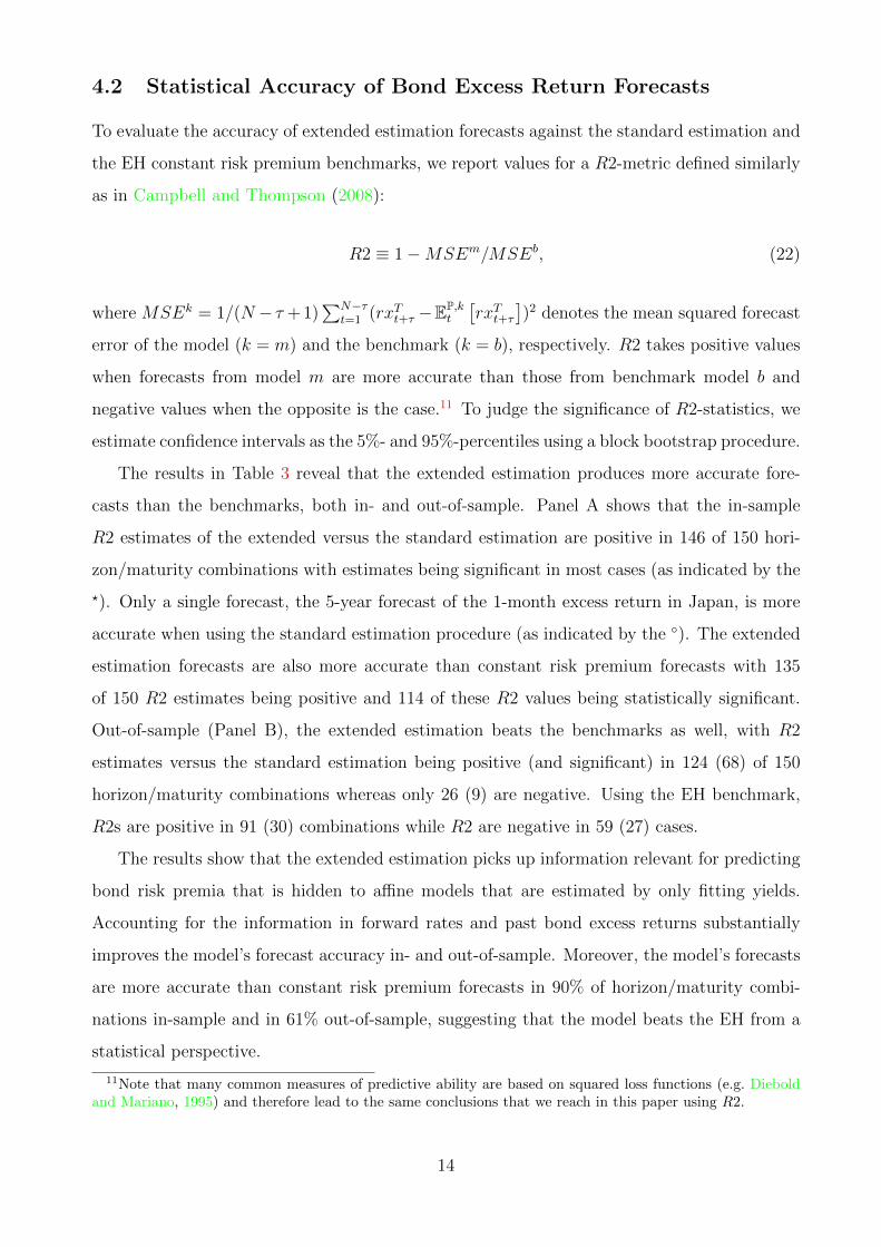
4.2 Statistical Accuracy of Bond Excess Return Forecasts

To evaluate the accuracy of extended estimation forecasts against the standard estimation and

the EH constant risk premium benchmarks, we report values for a R2-metric defined similarly

as in Campbell and Thompson (2008):

R2 ≡ 1−MSEm/MSEb, (22)

where MSEk = 1/(N − τ + 1)∑N−τ

t=1 (rxTt+τ −EP,kt

[rxTt+τ

])2 denotes the mean squared forecast

error of the model (k = m) and the benchmark (k = b), respectively. R2 takes positive values

when forecasts from model m are more accurate than those from benchmark model b and

negative values when the opposite is the case.11 To judge the significance of R2-statistics, we

estimate confidence intervals as the 5%- and 95%-percentiles using a block bootstrap procedure.

The results in Table 3 reveal that the extended estimation produces more accurate fore-

casts than the benchmarks, both in- and out-of-sample. Panel A shows that the in-sample

R2 estimates of the extended versus the standard estimation are positive in 146 of 150 hori-

zon/maturity combinations with estimates being significant in most cases (as indicated by the

?). Only a single forecast, the 5-year forecast of the 1-month excess return in Japan, is more

accurate when using the standard estimation procedure (as indicated by the ◦). The extended

estimation forecasts are also more accurate than constant risk premium forecasts with 135

of 150 R2 estimates being positive and 114 of these R2 values being statistically significant.

Out-of-sample (Panel B), the extended estimation beats the benchmarks as well, with R2

estimates versus the standard estimation being positive (and significant) in 124 (68) of 150

horizon/maturity combinations whereas only 26 (9) are negative. Using the EH benchmark,

R2s are positive in 91 (30) combinations while R2 are negative in 59 (27) cases.

The results show that the extended estimation picks up information relevant for predicting

bond risk premia that is hidden to affine models that are estimated by only fitting yields.

Accounting for the information in forward rates and past bond excess returns substantially

improves the model’s forecast accuracy in- and out-of-sample. Moreover, the model’s forecasts

are more accurate than constant risk premium forecasts in 90% of horizon/maturity combi-

nations in-sample and in 61% out-of-sample, suggesting that the model beats the EH from a

statistical perspective.

11Note that many common measures of predictive ability are based on squared loss functions (e.g. Dieboldand Mariano, 1995) and therefore lead to the same conclusions that we reach in this paper using R2.

14

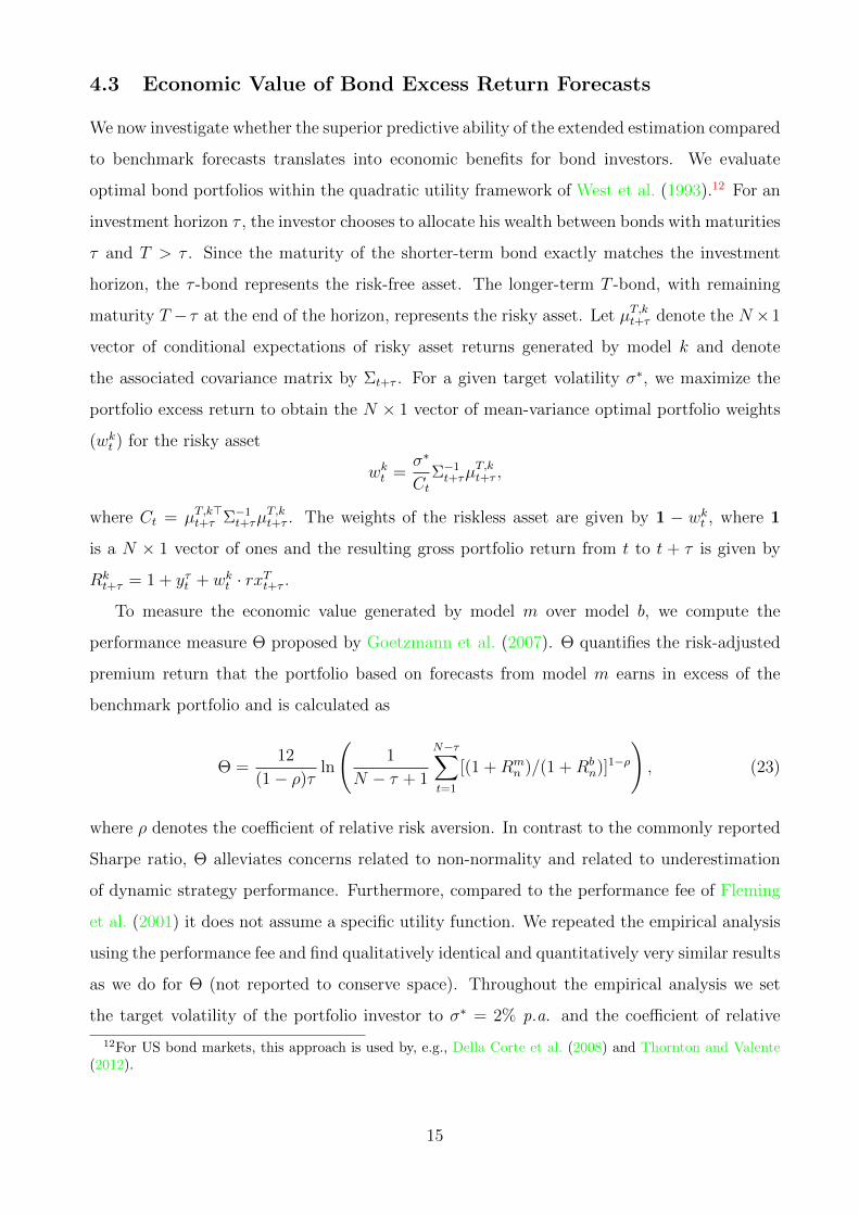
4.3 Economic Value of Bond Excess Return Forecasts

We now investigate whether the superior predictive ability of the extended estimation compared

to benchmark forecasts translates into economic benefits for bond investors. We evaluate

optimal bond portfolios within the quadratic utility framework of West et al. (1993).12 For an

investment horizon τ , the investor chooses to allocate his wealth between bonds with maturities

τ and T > τ . Since the maturity of the shorter-term bond exactly matches the investment

horizon, the τ -bond represents the risk-free asset. The longer-term T -bond, with remaining

maturity T − τ at the end of the horizon, represents the risky asset. Let µT,kt+τ denote the N ×1

vector of conditional expectations of risky asset returns generated by model k and denote

the associated covariance matrix by Σt+τ . For a given target volatility σ∗, we maximize the

portfolio excess return to obtain the N × 1 vector of mean-variance optimal portfolio weights

(wkt ) for the risky asset

wkt =σ∗

CtΣ−1t+τµ

T,kt+τ ,

where Ct = µT,k>t+τ Σ−1t+τµ

T,kt+τ . The weights of the riskless asset are given by 1 − wkt , where 1

is a N × 1 vector of ones and the resulting gross portfolio return from t to t + τ is given by

Rkt+τ = 1 + yτt + wkt · rxTt+τ .

To measure the economic value generated by model m over model b, we compute the

performance measure Θ proposed by Goetzmann et al. (2007). Θ quantifies the risk-adjusted

premium return that the portfolio based on forecasts from model m earns in excess of the

benchmark portfolio and is calculated as

Θ =12

(1− ρ)τln

(1

N − τ + 1

N−τ∑t=1

[(1 +Rmn )/(1 +Rb

n)]1−ρ

), (23)

where ρ denotes the coefficient of relative risk aversion. In contrast to the commonly reported

Sharpe ratio, Θ alleviates concerns related to non-normality and related to underestimation

of dynamic strategy performance. Furthermore, compared to the performance fee of Fleming

et al. (2001) it does not assume a specific utility function. We repeated the empirical analysis

using the performance fee and find qualitatively identical and quantitatively very similar results

as we do for Θ (not reported to conserve space). Throughout the empirical analysis we set

the target volatility of the portfolio investor to σ∗ = 2% p.a. and the coefficient of relative

12For US bond markets, this approach is used by, e.g., Della Corte et al. (2008) and Thornton and Valente(2012).

15

risk aversion to ρ = 3. All our results are robust to choosing different values of σ∗, varying ρ

between 2 and 6, as well as short sale constraints.

We report portfolio excess returns of investors using forecasts from the extended estimation

and performance measures relative to the standard estimation and EH forecasts in Table 4. The

results show that bond excess returns increase with the maturity of the longer-term bond and

decrease with prediction horizon. In-sample (Panel A), portfolio excess returns are positive

for all horizon/maturity combinations. Relative to the standard estimation, Θ values are

positive and suggest a superior performance in 127 out of 150 horizon/maturity combinations,

four Θ values are negative, and the remaining 19 estimates are zero. Premium returns in

excess of portfolios based on EH forecasts are also positive in 114 of the 150 horizon/maturity

combinations, while negative only for 11 of the combinations, suggesting a rejection of the EH

also in terms of economic significance. Θ estimates increase with the maturity of the longer-

term bond but decrease with prediction horizon, suggesting that, in particular, EH deviations

over longer horizons are of limited relevance in economic terms.

In the out-of-sample analysis (Panel B), we find that portfolios allocated based on ex-

tended estimation forecasts deliver positive excess returns in 140 of 150 horizon/maturity

combinations. Θ estimates relative to the standard estimation are positive in 123 of the 150

combinations. With the exception of Switzerland, we find that the economic value added by

the extended over the standard estimation tends to increase with bond maturity and to de-

crease with forecast horizon. For Switzerland, the standard estimation short-term forecasts

deliver higher portfolio returns for 3 out of 5 bond maturities but long-horizon investors earn

a risk-adjusted premium of 2% p.a. to 3% p.a. when they switch to the extended estimation

strategy. For all other countries, bond investors earn highest premium returns for short-horizon

long-term bond portfolios, ranging from approximately 2% p.a. to around 4.8% p.a. Rela-

tive to the EH, however, the Θ estimates are positive in only 39 of 150 cases, negative in 79

cases, and zero in 32 cases. Thus, in contrast to the statistical predictability results above,

these findings do not suggest that using extended estimation instead of constant risk premium

forecasts adds economic value for bond investors.

Overall, these results suggest that the information hidden to affine models estimated with

the standard procedure but captured through the extended procedure results in economic gains

for bond investors. Relative to the EH, however, bond investors only earn premium returns

in-sample whereas the EH cannot be outperformed - in an economic sense - out-of-sample.

16

4.4 Can anything beat the EH?

Our results show that extending ATSM estimations beyond fitting yields to additionally match

past excess returns captures information otherwise unspanned or hidden to standard ATSM

estimations (Duffee, 2011). The extension leads to a substantial improvement in forecast

accuracy for bond excess returns that translates into economic gains for portfolio investors

who would be willing to pay fees in the range of 2% p.a. to 4.8% p.a. to switch from the

standard to the extended estimation.

More generally, model risk premia generate unbiased bond excess return predictions that

entail high explanatory power for EH deviations; the average R2s of 79% for one-year excess

returns is beyond that of forward rate-based forecasts (Cochrane and Piazzesi, 2005). To

evaluate the EH postulate of constant risk premia, we use the historical average bond excess

return as a benchmark predictor. While the model beats EH forecasts in terms of statistical

accuracy in- and out-of-sample, investors do not gain economic value from model forecasts out-

of-sample. The finding that bond investors generally cannot benefit from using conditional risk

premia as compared to using the historical average can be viewed as the bond market analogue

to the result of Goyal and Welch (2008) for stock markets.

5 Discussion of Results, Extensions, and Robustness

Checks

We first show why statistical and economic criteria may lead to apparently conflicting con-

clusions about the validity of the EH. Subsequently, we discuss the potential benefits of aug-

menting ATSM estimations by imposing EH priors. Finally, we summarize various robustness

checks.

5.1 Statistical Accuracy versus Economic Value

While there are many papers on predictability of bond risk premia that are concerned with

statistical forecast accuracy, it is important to note that statistical accuracy per se does not

imply economic value for bond investors. Our results above indeed suggest that the EH is

rejected from a statistical but not from an economic value perspective: 61% of model forecasts

are more accurate than the EH but only 26% of forecasts add economic value. We present

general, model-free arguments as to why there may be a gap between statistical and economic

17

significance and evaluate our model results along these lines. These arguments are also useful

when interpreting the results of other papers that study the predictability of bond risk premia

using various forecasting approaches.

5.1.1 Economic Relevance of EH Deviations

One reason for apparently conflicting results is that departures from the EH might be statis-

tically significant but too small to be exploited by bond investors. In other words, failure to

generate economic value may not imply that a model fails to capture EH deviations accurately

but rather that the EH holds in an economic sense. Since there is no “natural” upper bound

for economic value measures (similar to a regression R2 capped by one or forecast errors floored

by zero), we compare the economic performance of model forecasts to the performance of the

same strategy under perfect foresight. If perfect foresight returns of the strategy are high but

the model evaluated only captures a (small) fraction of these excess returns, EH deviations

are not exploited because the model fails. If the model captures a large fraction of perfect

foresight returns but returns are nevertheless economically small, this suggest that “true” EH

deviations are indeed economically irrelevant.13, 14

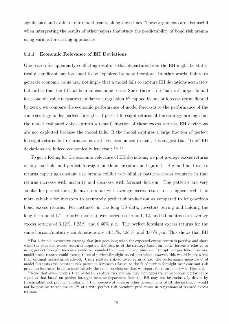
To get a feeling for the economic relevance of EH deviations, we plot average excess returns

of buy-and-hold and perfect foresight portfolio investors in Figure 1. Buy-and-hold excess

returns capturing constant risk premia exhibit very similar patterns across countries in that

returns increase with maturity and decrease with forecast horizon. The patterns are very

similar for perfect foresight investors but with average excess returns on a higher level. It is

more valuable for investors to accurately predict short-horizon as compared to long-horizon

bond excess returns. For instance, in the long US data, investors buying and holding the

long-term bond (T − τ = 60 months) over horizons of τ = 1, 12, and 60 months earn average

excess returns of 3.12%, 1.25%, and 0.40% p.a.. The perfect foresight excess returns for the

same horizon/maturity combinations are 14.41%, 4.83%, and 3.05% p.a. This shows that EH

13For a simple investment strategy that just goes long when the expected excess return is positive and shortwhen the expected excess return is negative, the returns of the strategy based on model forecasts relative tousing perfect foresight forecasts would be bounded by minus one and plus one. For optimal portfolio investors,model-based returns could exceed those of perfect-foresight-based portfolios; however, this would imply a lessthan optimal risk-return-trade-off. Using relative risk-adjusted returns, i.e. the performance measure Θ ofmodel forecasts over constant risk premium forecasts relative to the Θ of perfect foresight over constant riskpremium forecasts, leads to qualitatively the same conclusions that we report for returns below in Figure 2.

14Note that even models that perfectly capture risk premia may not generate an economic performanceequal to that based on perfect foresight because departures from the EH may not be exclusively driven by(predictable) risk premia. Similarly, in the presence of noise or other determinants of EH deviations, it wouldnot be possible to achieve an R2 of 1 with perfect risk premium predictions in regressions of realized excessreturns.

18

deviations are economically less important for increasing τ and, as a consequence, having a less

then perfect forecast model for short horizons may add more economic value than a perfect

forecast model for longer horizons.

In Figure 2, we plot the excess returns of portfolios allocated using forecasts based on

constant risk premia (in green), the standard estimation (in red), and the extended estimation

(in black) relative to perfect foresight portfolio returns. The graphs show that EH deviations

are not as important economically as statistical results might suggest: EH-consistent constant

risk premium forecasts capture a large fraction (increasing with horizon) of perfect foresight

returns. The extended estimation forecasts capture a larger fraction of perfect foresight returns

than standard estimation forecasts. The fraction of perfect foresight returns captured by

extended estimation forecasts generally increases with horizons, similar to the regression R2s

in Table 2 and R2-statistics in Table 3. In contrast, the economic value measures reported in

Table 4 decrease with horizon, consistent with comparably lower statistical accuracy at short

horizons adding higher economic value than more accurate forecasts for longer horizons at

which EH deviations are not relevant in economic terms. In other words, statistical accuracy

cannot lead to economic value when EH deviations are too small to be exploited by investors.15

5.1.2 Information in Economic Value versus Statistical Accuracy Measures

Conflicting conclusions based on metrics of statistical accuracy and economic value may also

result from the construction of the measures used. Common measures of predictive ability

are based on loss functions involving squared or absolute forecast errors and – by definition –

ignore the sign of forecast errors. Getting the sign right, however, is of utmost importance for

investors since the sign of the forecast determines whether to take a long or a short position. To

illustrate this point, consider two competing forecasts of excess returns being -1% and 8% and

suppose the realization is 2%. Standard measures of predictive ability consider the forecast of

-1% more accurate because the absolute error is just half of that of the 8% forecast. In terms

of investment performance, however, the first forecast would have resulted in a loss while the

second would have resulted in a positive performance.

As a measure of directional accuracy, we compute hit ratios measuring the fraction of

correctly signed forecasts. Table 5 reports the hit ratios of the extended estimation relative to

15Consider, for instance, the one-year out-of-sample forecasts in Japan: extended estimation forecasts havehigh accuracy (R2 from 0.11 to 0.70), capture more than 90% of perfect foresight returns, but their the economicvalue is close to zero (-2 to +7 basis points p.a.) because EH deviations are very small and constant risk premiaalready capture around 80% of perfect foresight performance.

19

the hit ratios of constant risk premium forecasts, with asterisks (circles) indicating that model

hit ratios are significantly higher (lower) than those of constant risk premium forecasts. While

the model generally has high directional accuracy in-sample, model hit ratios exceed constant

risk premium hit ratios only in 49 of the 150 horizon/maturity combinations out-of-sample.

This contrasts with the R2 results in Table 3 where 91 of 150 combinations suggested that

the model has higher predictive ability compared to constant risk premium forecasts. Thus,

our finding that the economic value analysis is more in favor of the EH than the statistical

accuracy results can partly be explained by forecasts having small squared/absolute errors but

nonetheless pointing in the wrong direction.16

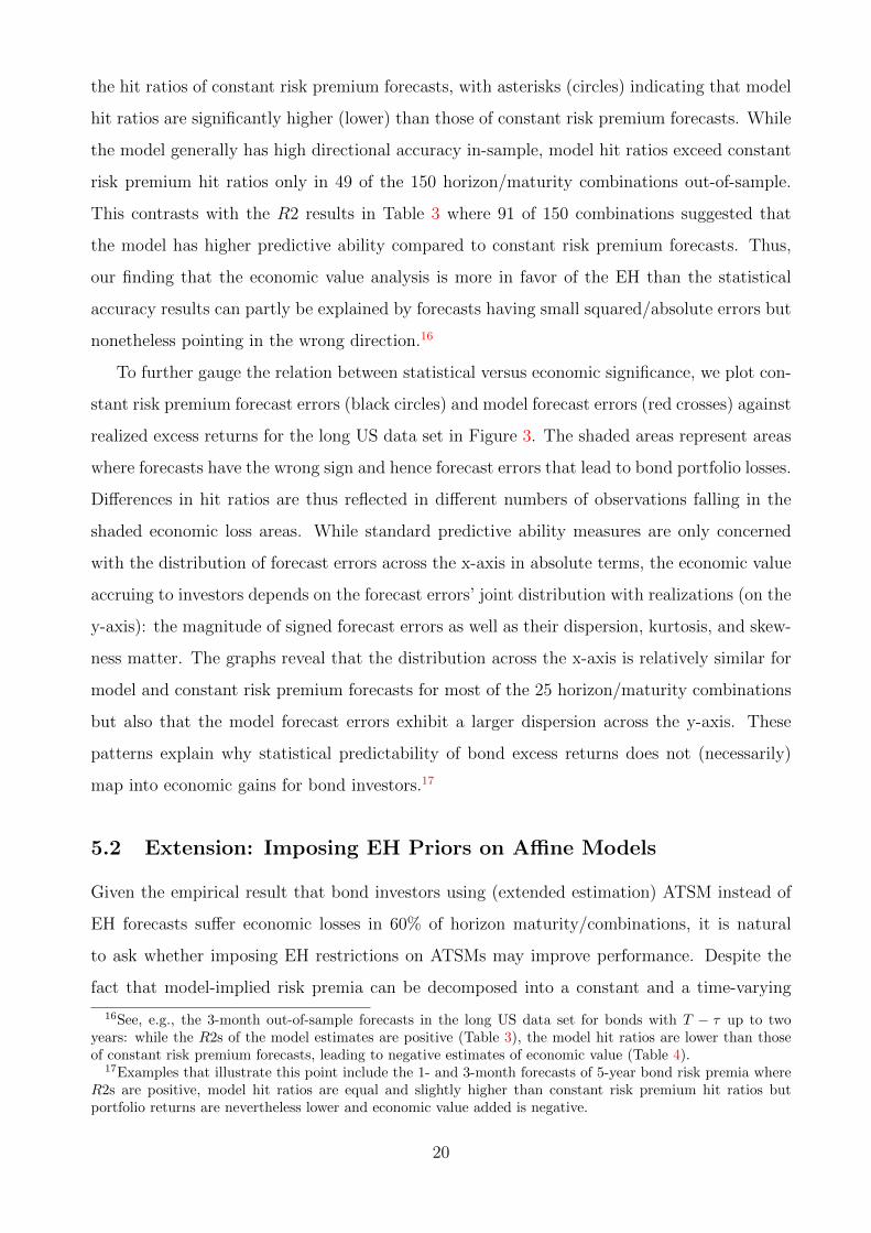
To further gauge the relation between statistical versus economic significance, we plot con-

stant risk premium forecast errors (black circles) and model forecast errors (red crosses) against

realized excess returns for the long US data set in Figure 3. The shaded areas represent areas

where forecasts have the wrong sign and hence forecast errors that lead to bond portfolio losses.

Differences in hit ratios are thus reflected in different numbers of observations falling in the

shaded economic loss areas. While standard predictive ability measures are only concerned

with the distribution of forecast errors across the x-axis in absolute terms, the economic value

accruing to investors depends on the forecast errors’ joint distribution with realizations (on the

y-axis): the magnitude of signed forecast errors as well as their dispersion, kurtosis, and skew-

ness matter. The graphs reveal that the distribution across the x-axis is relatively similar for

model and constant risk premium forecasts for most of the 25 horizon/maturity combinations

but also that the model forecast errors exhibit a larger dispersion across the y-axis. These

patterns explain why statistical predictability of bond excess returns does not (necessarily)

map into economic gains for bond investors.17

5.2 Extension: Imposing EH Priors on Affine Models

Given the empirical result that bond investors using (extended estimation) ATSM instead of

EH forecasts suffer economic losses in 60% of horizon maturity/combinations, it is natural

to ask whether imposing EH restrictions on ATSMs may improve performance. Despite the

fact that model-implied risk premia can be decomposed into a constant and a time-varying

16See, e.g., the 3-month out-of-sample forecasts in the long US data set for bonds with T − τ up to twoyears: while the R2s of the model estimates are positive (Table 3), the model hit ratios are lower than thoseof constant risk premium forecasts, leading to negative estimates of economic value (Table 4).

17Examples that illustrate this point include the 1- and 3-month forecasts of 5-year bond risk premia whereR2s are positive, model hit ratios are equal and slightly higher than constant risk premium hit ratios butportfolio returns are nevertheless lower and economic value added is negative.

20

component, see Eq. (15), it can be shown that it is not possible to impose parametric EH

restrictions on ATSMs in general, but only in special cases that are very restrictive and hinder

realistic modeling.18 In a Bayesian setting, however, the EH can be imposed in a “soft way”,

through a prior distribution rather than a hard parameter restriction. Consider

log π(θQP) ∝ −1

2γτ ,T (θQP)Ξγτ ,T (θQP)>, (24)

with Ξ positive semi-definite. Depending on the specification of Ξ, this prior arbitrarily reduces

or amplifies, for a given sample path of the latent state variables, the time-variability of risk

premia across maturities. More specifically, the prior imposes a penalty on γ, the coefficient

that controls the time-variation of expected excess returns in Eq. (15), with the penalty

increasing in the determinant of Ξ. Intuitively, the prior should prevent overfitting (Duffee,

2010) and alleviate related concerns on parameter uncertainty (Feldhutter et al., 2012): while

the prior does not directly restrict the variance of expected risk premia (which also depends

on the variance of the state variables), it penalizes all parameters constellations that make

expected risk premia excessively time-varying. This approach can be viewed as a soft version

of excluding economically unrealistic model outputs, in the spirit of Duffee (2010).

In a preliminary exercise, we repeat the out-of-sample analysis for the long US data set

using the extended estimation procedure with a “weak” and a “strong” EH prior and present

results in Table 6.19 Imposing the weak EH prior (Panel A) substantially augments predictive

accuracy for horizons of one year or longer and leads to higher hit ratios in 24 of 25 hori-

zon/maturity combinations compared to the estimation without prior; in nine cases these hit

ratios exceed those using constant risk premium forecasts. Furthermore, there is an increase in

bond portfolio excess returns and in economic value across horizons and maturities. While for

the estimation without prior all Θ estimates are negative (reported above in Table 4), we find

positive estimates for ten horizon/maturity combinations with the weak prior. Nevertheless,

the economic value added by conditioning on an affine model instead of constant risk premium

forecasts is on average very small.

For the strong EH prior, we also find that predictive accuracy improves for horizons of one

18First, the pure EH can be imposed when the term structure is flat and mean reversion in the state variablesis infinitely fast. Infinite speed of mean reversion is in strong contrast to the empirical observation that interestrates are very persistent. Second, the EH can be imposed on a subset of yields by numerically finding the rootsof γ and η from Eqs. (13) and (14), but not the entire yield curve. Proofs are omitted from the paper butavailable on request.

19We define the “weak” and “strong” prior with Ξ identity matrix times 10,000 and times 1e12, respectively.

21

year and beyond. The R2-statistics are comparably small in absolute value, suggesting that

model and constant risk premium forecasts errors are of similar magnitude. The hit ratios

are very similar to those using constant risk premia, being equal in eleven cases and slightly

higher or lower in seven cases each. Bond portfolio returns and economic value increase with the

imposition of the strong EH prior, and the Θ estimates averaged across horizons and maturities

are slightly positive (albeit often close to zero). Finding that the predictive accuracy and hit

ratios of strong EH prior and constant risk premium forecasts are very similar and that the

economic value is close to zero illustrates how one can approach the aforementioned “soft”

imposition of the EH on ATSMs in our Bayesian setup.20

Overall, we find that imposing EH priors increases the economic value generated by ATSM

forecasts. We leave the precise specification of the prior that balances EH-imposed penalties

versus variability in risk premia for future research.

5.3 Robustness Checks

We now summarize various robustness checks that support our findings. The results are not

reported to save space but available from the authors on request.

5.3.1 Alternative Yield Data

We use bond prices (from Datastream) directly to estimate zero yields using the approaches

of Nelson and Siegel (1987) and Svensson (1994), as well as the smoothed and unsmoothed

versions of the Fama and Bliss (1987) method. The results are qualitatively identical to those

reported above. We also use term structure data provided by central banks (for countries where

data is available) and reach the same conclusions. Thus, our findings do not depend on the

mechanism used to estimate the zero curve in general and, more specifically, our conclusions

are not affected by credit risk issues that have become relevant in Libor and swap markets

during the recent crisis. The latter argument is also supported by the results reported above

for the US yield data set from 1952 to 2003 since this data does not involve Libor or swap

rates and the sample ends well before the recent crisis.

20Given such a soft imposition of the EH, one might also consider testing the EH in a generalized version ofthe bivariate VAR framework of Bekaert and Hodrick (2001) using ATSMs to jointly model not only a pair ofyields but the full term structure (under no-arbitrage).

22

5.3.2 Alternative ATSM Specifications

We verify that our conclusions are robust to changes in the ATSM specification and repeat

the empirical analysis using a larger model with four factors (A0(4) model) and a stochastic

volatility model (A1(3) model). In general, changing the specification can have an impact

on yield pricing errors and/or forecast accuracy. We find that changing the specification

may improve or deteriorate particular results but the overall picture does not change and our

conclusions remain the same.

5.3.3 Forecasting Bond Excess Returns with Forward Rates

Previous research documents (in-sample) predictability of bond excess returns using lagged

forward rates; see e.g. Fama and Bliss (1987) and Cochrane and Piazzesi (2005, CP). While

we do not impose the CP-factor in the model structure, the extended estimation procedure

that matches model risk premia to the data incorporates forward rates that the CP-factor is

based upon and it additionally accounts for past forecast errors. In line with previous research,

we find that forward rates contain information for in-sample predictions of bond excess returns

but do not generate economic value out-of-sample (Thornton and Valente, 2012). Forecasts

based on the extended ATSM estimation proposed in this paper have larger predictive ability

and add more economic value than the CP-factor forecasts in- and out-of-sample, thus, posing

a stronger challenge to the EH and thereby providing more general findings.

6 Conclusion

In this paper, we offer new insights on the validity of the expectations hypothesis (EH) by

studying the economic benefits that accrue to bond investors who exploit predictable devi-

ations from the EH. We estimate conditional bond risk premia using affine term structure

models (ATSMs) by employing a novel estimation strategy that jointly fits the term struc-

ture of model yields to the observed yield curve and additionally matches model risk premia

with bond excess returns observed in the past. This extended procedure allows investors to

capture predictive information beyond the cross section of yields and to update beliefs about

the model’s predictive ability based on its past performance. We use the model to generate

forecasts of bond excess returns and, based on these forecasts, we determine optimal bond

portfolios. To evaluate the model against the EH, we compare the model’s forecast accuracy

23

and corresponding portfolio performance to EH-consistent forecasts and accordingly allocated

benchmark portfolios, where we use averages of historical bond excess returns to consistently

estimate constant risk premia as postulated by the EH.

We find that, for 25 combinations of horizons and maturities ranging from one month to

ten years, bond risk premia have very similar properties across countries, leading to uniform

conclusions for the US, Switzerland, Germany, the UK, and Japan. We show that the extended

estimation captures predictive information otherwise hidden to standard ATSM estimations,

thereby providing investors with forecasts that are statistically more accurate and economi-

cally more valuable; out-of-sample, investors would be willing to pay an annual premium in

the range of 2% to 4.8% to switch from the standard to the extended estimation procedure.

More generally, regressing realized on model-implied excess returns reveals that extended es-

timation forecasts are unbiased and have high explanatory power with R2s of about 26% at

the one-month prediction horizon and about 79% at the one-year horizon. From a statistical

perspective, the model beats the EH forecasts of constant risk premia as judged by standard

metrics of predictive accuracy in- and out-of-sample. Furthermore, portfolios allocated based

on the extended estimation forecasts earn positive excess returns; however, out-of-sample these

portfolios perform worse than the corresponding EH benchmark portfolios. In other words,

investors cannot beat the historical average, which suggests that our findings can be viewed

as a bond market analogue to Goyal and Welch (2008).

At first sight, our results may appear to offer conflicting conclusions for statistical and eco-

nomic assessments of the EH. We show that this finding is not rooted in the use of ATSMs but

potentially applies to any approach for modeling and predicting bond risk premia. We demon-

strate that there is a wedge between the statistical and economic relevance of EH deviations

for two reasons. First, departures from the EH can be statistically significant but too small

to be exploited by investors, in particular over longer horizons. Second, metrics of statistical

accuracy evaluate loss functions that are in many respects unrelated to the economic success

of bond investments. As such, even models with high regression R2s or measures of predic-

tive ability per se cannot guarantee to provide bond investors with economic gains relative to

presuming that the EH holds.

Overall, our results suggest that the EH presumption of constant risk premia, while being

statistically rejected by the data, still provides a good first approximation to the out-of-sample

behavior of bond excess returns for the purpose of asset allocation in fixed income markets,

especially so over long forecast horizons. This finding is in line with the EH, despite being cen-

24

turies old, having remained a benchmark for a number of practical purposes in many financial

firms and policy institutions, e.g. for extracting information about future inflation, interest

rates, and economic activity. At the same time, ATSMs are well established in the literature

because of their virtues in modeling interest rates. Taken together, these insights suggest to

examine models of bond risk premia that grant flexibility in their specification but account

for the EH as an anchor. As a first step in this direction, we consider ATSMs on which we

impose the EH through priors in the estimation in order to limit (excessive) variability of risk

premia. The results of this preliminary exercise suggest that imposing EH priors improves the

performance of bond portfolios and we leave it to future research to further explore modeling

and estimation approaches that balance flexibility and economically reasonable restrictions.

25

References

Aıt-Sahalia, Y., Hansen, L. P. (Eds.), 2009, Handbook of Financial Econometrics, Else-vier.

Almeida, C., Graveline, J., Joslin, S., 2011, “Do interest rate options contain informationabout excess returns?,” Journal of Econometrics, 164, 35–44.

Andrews, D., 1991, “Heteroskedasticity and Autocorrelation Consistent Covariance MatrixEstimation,” Econometrica, 59, 817–858.

Backus, D. K., Foresi, S., Mozumdar, A., Wu, L., 2001, “Predictable changes in yields andforward rates,” Journal of Financial Economics, 59, 281–311.

Barberis, N., 2000, “Investing for the Long Run when Returns Are Predictable,” Journal ofFinance, 55, 225–264.

Bekaert, G., Hodrick, R. J., 2001, “Expectations Hypotheses Tests,” Journal of Finance, 56,1357–1394.

Bekaert, G., Hodrick, R. J., Marshall, D., 1997, “The Implications of First-Order Risk Aversionfor Asset Market Risk Premiums,” Journal of Monetary Economics, 40, 3–39.

Campbell, J. Y., Shiller, R. J., 1991, “Yield Spreads and Interest Rate Movements: A Bird’sEye View,” Review of Economic Studies, 58, 495–514.

Campbell, J. Y., Thompson, S. B., 2008, “Predicting Excess Stock Returns Out of Sample:Can Anything Beat the Historical Average?,” Review of Financial Studies, 21, 1509–1531.

Cheridito, P., Filipovic, D., Kimmel, R., 2007, “Market Price of Risk Specifications for AffineModels: Theory and Evidence,” Journal of Financial Economics, 83, 123–170.

Cieslak, A., Povala, P., 2011, “Understanding bond risk premia,” Working Paper, Northwest-ern.

Cochrane, J., Piazzesi, M., 2005, “Bond Risk Premia,” American Economic Review, 95, 138–160.

Dai, Q., Singleton, K. J., 2000, “Specification Analysis of Affine Term Structure Models,”Journal of Finance, 55, 1943–1978.

Dai, Q., Singleton, K. J., 2002, “Expectation puzzles, time-varying risk premia, and affinemodels of the term structure,” Journal of Financial Economics, 63, 415–441.

Della Corte, P., Sarno, L., Thornton, D. L., 2008, “The expectation hypothesis of the termstructure of very short-term rates: Statistical tests and economic value,” Journal of Finan-cial Economics, 89, 158–174.

Diebold, F. X., Mariano, R. S., 1995, “Comparing Predictive Accuracy,” Journal of Business& Economic Statistics, 13, 253–263.

Duffee, G., 2010, “Sharpe Ratios in Term Structure Models,” Working paper, Johns HopkinsUniversity.

26

Duffee, G., 2011, “Information in (and not in) the term structure,” Review of Financial Studies,24, 2895–2934.

Duffie, D., Filipovic, D., Schachermayer, W., 2003, “Affine Processes and Applications inFinance,” Annals of Applied Probability, 13, 984–1053.

Duffie, D., Kan, R., 1996, “A Yield-Factor Model of Interest Rates,” Mathematical Finance,6, 379–406.

Fama, E. F., 1984, “The information in the term structure,” Journal of Financial Economics,13, 509–528.

Fama, E. F., Bliss, R. R., 1987, “The Information in Long-Maturity Forward Rates,” AmericanEconomic Review, 77, 680–692.

Feldhutter, P., Lando, D., 2008, “Decomposing Swap Spreads,” Journal of Financial Eco-nomics, 88, 375–405.

Feldhutter, P., Larsen, L., Munk, C., Trolle, A., 2012, “Keep it simple: Dynamic bond port-folios under parameter uncertainty,” Working Paper, London Business School.

Filipovic, D., Mayerhofer, E., Schneider, P., 2013, “Density Approximations for MultivariateAffine Jump-Diffusion Processes,” Journal of Econometrics, forthcoming.

Fisher, I., 1896, “Appreciation and Interest,” Publications of the American Economic Associ-ation, 9, 331–442.

Fisher, I., 1930, The Theory of Interest, The Macmillan Co., New York.

Fisher, M., Gilles, C., 1996a, “Estimating Exponential-Affine Models of the Term Structure,”Working paper, Federal Reserve Board.

Fisher, M., Gilles, C., 1996b, “Term Premia in Exponential Affine Models of the Term Struc-ture,” Working paper, Federal Reserve Board.

Fleming, J., Kirby, C., Ostdiek, B., 2001, “The Economic Value of Volatility Timing,” Journalof Finance, 56, 329–352.

Goetzmann, W., Ingersoll, J., Spiegel, M., Welch, I., 2007, “Portfolio Performance Manip-ulation and Manipulation-proof Performance Measures,” Review of Financial Studies, 20,1503–1546.

Goh, J., Jiang, F., Tu, J., Zhou, G., 2012, “Forecasting Government Bond Risk Premia UsingTechnical Indicators,” Working Paper, SMU.

Goyal, A., Welch, I., 2008, “A Comprehensive Look at the Empirical Performance of EquityPremium Prediction,” Review of Financial Studies, 21, 1455–1508.

Gurkaynak, R. S., Sack, B., Wright, J. H., 2007, “The U.S. Treasury yield curve: 1961 to thepresent,” Journal of Monetary Economics, 54, 2291–2304.

Hicks, J., 1953, Value and Capital, Oxford University Press, London.

Joslin, S., Priebsch, M., Singleton, K., 2010, “Risk Premiums in Dynamic Term StructureModels with Unspanned Macro Risks,” Working Paper, Stanford University.

27

Joslin, S., Singleton, K., Zhu, H., 2011, “A New Perspective on Gaussian Dynamic TermStructure Models,” Review of Financial Studies, 24, 926–970.

Keynes, J. M., 1930, A Treatise on Money, The Macmillan Co., London.

Litterman, R., Scheinkman, J. A., 1991, “Common Factors Affecting Bond Returns,” Journalof Fixed Income, 1, 54–61.

Ludvigson, S., Ng, S., 2009, “Macro Factors in Bond Risk Premia,” Review of FinancialStudies, 22, 5027–5067.

Lutz, F. A., 1940, “The Structure of Interest Rates,” Quarterly Journal of Economics, 55,36–63.

Mueller, P., Vedolin, A., Zhou, H., 2011, “Short Run Bond Risk Premia,” Discussion Paper686, Financial Markets Group, LSE.

Nelson, C. R., Siegel, A. F., 1987, “Parsimonious Modeling of Yield Curves,” Journal ofBusiness, 60, 473–489.

Newey, W., West, K., 1987, “A Simple Positive Semi-Definite, Heteroscedasticity and Autor-correlation Consitent Covariance Matrix,” Econometrica, 55, 703–708.

Sarno, L., Thornton, D. L., Valente, G., 2007, “The Empirical Failure of the ExpectationsHypothesis of the Term Structure of Bond Yields,” Journal of Financial and QuantitativeAnalysis, 42, 81–100.

Svensson, L., 1994, “Estimating and Interpreting Forward Interest Rates: Sweden 1992 - 1994,”NBER Working Paper 4871.

Tang, H., Xia, Y., 2007, “An International Examination of Affine Term Structure Models andthe Expectations Hypothesis,” Journal of Financial and Quantitative Analysis, 42, 41–80.

Thornton, D., Valente, G., 2012, “Out-of-sample predictions of bond excess returns and for-ward rates: an asset allocation perspective,” Review of Financial Studies, Forthcoming.

West, K., Edison, H., Cho, D., 1993, “A Utility Based Comparison of Exchange Rate Volatil-ity,” Journal of International Economics, 35, 23–45.

28

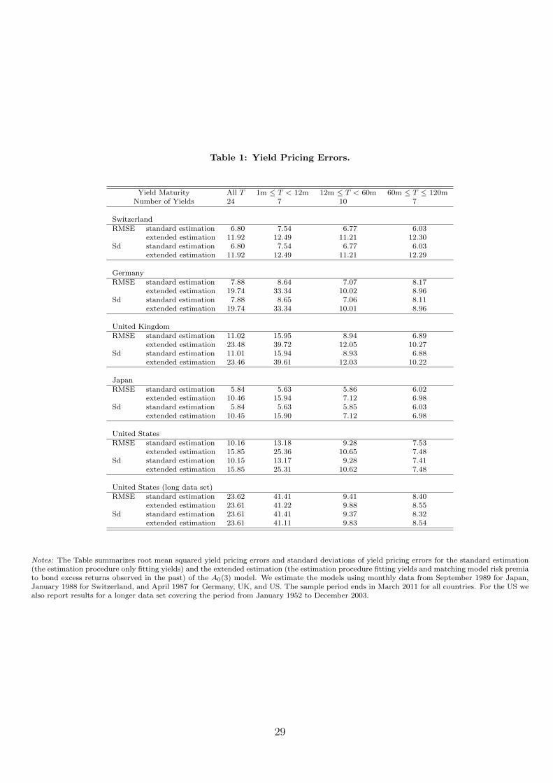
Table 1: Yield Pricing Errors.

Yield Maturity All T 1m ≤ T < 12m 12m ≤ T < 60m 60m ≤ T ≤ 120mNumber of Yields 24 7 10 7

SwitzerlandRMSE standard estimation 6.80 7.54 6.77 6.03

extended estimation 11.92 12.49 11.21 12.30Sd standard estimation 6.80 7.54 6.77 6.03

extended estimation 11.92 12.49 11.21 12.29

GermanyRMSE standard estimation 7.88 8.64 7.07 8.17

extended estimation 19.74 33.34 10.02 8.96Sd standard estimation 7.88 8.65 7.06 8.11

extended estimation 19.74 33.34 10.01 8.96

United KingdomRMSE standard estimation 11.02 15.95 8.94 6.89

extended estimation 23.48 39.72 12.05 10.27Sd standard estimation 11.01 15.94 8.93 6.88

extended estimation 23.46 39.61 12.03 10.22

JapanRMSE standard estimation 5.84 5.63 5.86 6.02

extended estimation 10.46 15.94 7.12 6.98Sd standard estimation 5.84 5.63 5.85 6.03

extended estimation 10.45 15.90 7.12 6.98

United StatesRMSE standard estimation 10.16 13.18 9.28 7.53

extended estimation 15.85 25.36 10.65 7.48Sd standard estimation 10.15 13.17 9.28 7.41

extended estimation 15.85 25.31 10.62 7.48

United States (long data set)RMSE standard estimation 23.62 41.41 9.41 8.40

extended estimation 23.61 41.22 9.88 8.55Sd standard estimation 23.61 41.41 9.37 8.32

extended estimation 23.61 41.11 9.83 8.54

Notes: The Table summarizes root mean squared yield pricing errors and standard deviations of yield pricing errors for the standard estimation(the estimation procedure only fitting yields) and the extended estimation (the estimation procedure fitting yields and matching model risk premiato bond excess returns observed in the past) of the A0(3) model. We estimate the models using monthly data from September 1989 for Japan,January 1988 for Switzerland, and April 1987 for Germany, UK, and US. The sample period ends in March 2011 for all countries. For the US wealso report results for a longer data set covering the period from January 1952 to December 2003.

29

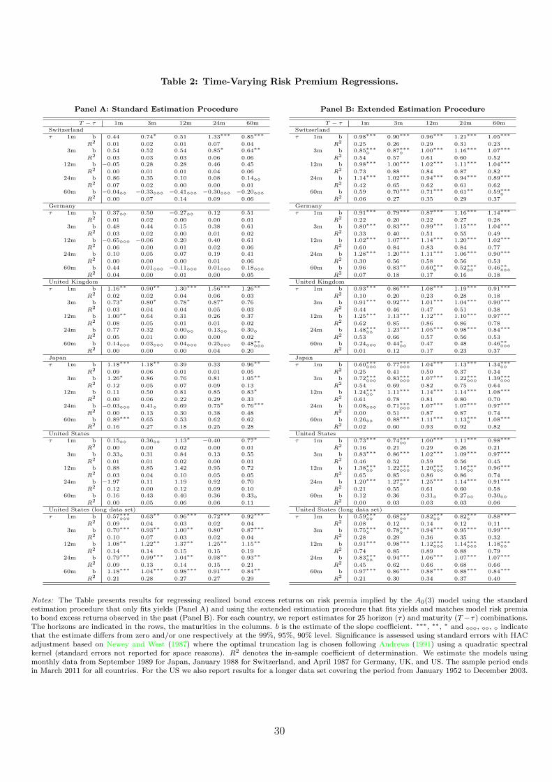
Table 2: Time-Varying Risk Premium Regressions.

Panel A: Standard Estimation Procedure

T − τ 1m 3m 12m 24m 60mSwitzerlandτ 1m b 0.44 0.74∗ 0.51 1.33∗∗∗ 0.85∗∗∗

R2 0.01 0.02 0.01 0.07 0.043m b 0.54 0.52 0.54 0.85∗ 0.64∗∗

R2 0.03 0.03 0.03 0.06 0.0612m b −0.05 0.28 0.28 0.46 0.45

R2 0.00 0.01 0.01 0.04 0.0624m b 0.86 0.35 0.10 0.08 0.14��

R2 0.07 0.02 0.00 0.00 0.0160m b −0.04�� −0.33��� −0.41��� −0.30��� −0.20���

R2 0.00 0.07 0.14 0.09 0.06Germanyτ 1m b 0.37�� 0.50 −0.27�� 0.12 0.51

R2 0.01 0.02 0.00 0.00 0.013m b 0.48 0.44 0.15 0.38 0.61

R2 0.03 0.02 0.00 0.01 0.0212m b −0.65��� −0.06 0.20 0.40 0.61

R2 0.06 0.00 0.01 0.02 0.0624m b 0.10 0.05 0.07 0.19 0.41

R2 0.00 0.00 0.00 0.01 0.0660m b 0.44 0.01��� −0.11��� 0.01��� 0.18���

R2 0.04 0.00 0.01 0.00 0.05United Kingdomτ 1m b 1.16∗∗ 0.90∗∗ 1.30∗∗∗ 1.56∗∗∗ 1.26∗∗

R2 0.02 0.02 0.04 0.06 0.033m b 0.73∗ 0.80∗ 0.78∗ 0.87∗ 0.76

R2 0.03 0.04 0.04 0.05 0.0312m b 1.00∗∗ 0.64 0.31 0.26 0.37

R2 0.08 0.05 0.01 0.01 0.0224m b 0.77 0.32 0.00�� 0.13�� 0.30�

R2 0.05 0.01 0.00 0.00 0.0260m b 0.14��� 0.03��� 0.04��� 0.25��� 0.48∗∗���

R2 0.00 0.00 0.00 0.04 0.20Japanτ 1m b 1.18∗∗∗ 1.18∗∗ 0.39 0.33 0.96∗∗

R2 0.09 0.06 0.01 0.01 0.053m b 1.26∗ 0.86 0.76 0.81 1.05∗∗

R2 0.12 0.05 0.07 0.09 0.1312m b 0.11 0.50 0.81 0.85 0.83∗

R2 0.00 0.06 0.22 0.29 0.3324m b −0.03��� 0.41� 0.69 0.75∗ 0.76∗∗∗

R2 0.00 0.13 0.30 0.38 0.4860m b 0.89∗∗∗ 0.65 0.53 0.62 0.62

R2 0.16 0.27 0.18 0.25 0.28United Statesτ 1m b 0.15�� 0.36�� 1.13∗ −0.40 0.77∗

R2 0.00 0.00 0.02 0.00 0.013m b 0.33� 0.31 0.84 0.13 0.55

R2 0.01 0.01 0.02 0.00 0.0112m b 0.88 0.85 1.42 0.95 0.72

R2 0.03 0.04 0.10 0.05 0.0524m b −1.97 0.11 1.19 0.92 0.70

R2 0.12 0.00 0.12 0.09 0.1060m b 0.16 0.43 0.40 0.36 0.33�

R2 0.00 0.05 0.06 0.06 0.11United States (long data set)τ 1m b 0.57∗∗∗��� 0.63∗∗ 0.96∗∗∗ 0.72∗∗∗ 0.92∗∗∗

R2 0.09 0.04 0.03 0.02 0.043m b 0.70∗∗∗ 0.93∗∗ 1.00∗∗ 0.80∗ 0.87∗∗∗

R2 0.10 0.07 0.03 0.02 0.0412m b 1.08∗∗ 1.22∗∗ 1.37∗∗ 1.25∗∗ 1.15∗∗

R2 0.14 0.14 0.15 0.15 0.1924m b 0.79∗∗∗ 0.99∗∗∗ 1.04∗∗ 0.98∗∗ 0.93∗∗

R2 0.09 0.13 0.14 0.15 0.2160m b 1.18∗∗∗ 1.04∗∗∗ 0.98∗∗∗ 0.91∗∗∗ 0.84∗∗

R2 0.21 0.28 0.27 0.27 0.29

Panel B: Extended Estimation Procedure

T − τ 1m 3m 12m 24m 60mSwitzerlandτ 1m b 0.98∗∗∗ 0.90∗∗∗ 0.96∗∗∗ 1.21∗∗∗ 1.05∗∗∗

R2 0.25 0.26 0.29 0.31 0.233m b 0.85∗∗∗� 0.87∗∗∗� 1.00∗∗∗ 1.16∗∗∗ 1.07∗∗∗

R2 0.54 0.57 0.61 0.60 0.5212m b 0.98∗∗∗ 1.00∗∗∗ 1.02∗∗∗ 1.11∗∗∗ 1.04∗∗∗

R2 0.73 0.88 0.84 0.87 0.8224m b 1.14∗∗∗ 1.02∗∗∗ 0.94∗∗∗ 0.94∗∗∗ 0.89∗∗∗

R2 0.42 0.65 0.62 0.61 0.6260m b 0.59 0.70∗∗∗ 0.71∗∗∗ 0.61∗∗ 0.59∗∗∗�

R2 0.06 0.27 0.35 0.29 0.37Germanyτ 1m b 0.91∗∗∗ 0.79∗∗∗ 0.87∗∗∗ 1.16∗∗∗ 1.14∗∗∗

R2 0.22 0.20 0.22 0.27 0.283m b 0.80∗∗∗ 0.83∗∗∗ 0.99∗∗∗ 1.15∗∗∗ 1.04∗∗∗

R2 0.33 0.40 0.51 0.55 0.4912m b 1.02∗∗∗ 1.07∗∗∗ 1.14∗∗∗ 1.20∗∗∗ 1.02∗∗∗

R2 0.60 0.84 0.83 0.84 0.7724m b 1.28∗∗∗ 1.20∗∗∗ 1.11∗∗∗ 1.06∗∗∗ 0.90∗∗∗

R2 0.30 0.56 0.58 0.56 0.5360m b 0.96 0.83∗∗ 0.60∗∗∗� 0.52∗∗∗�� 0.46∗∗���

R2 0.07 0.18 0.17 0.16 0.18United Kingdomτ 1m b 0.93∗∗∗ 0.86∗∗∗ 1.08∗∗∗ 1.19∗∗∗ 0.91∗∗∗

R2 0.10 0.20 0.23 0.28 0.183m b 0.91∗∗∗ 0.92∗∗∗ 1.01∗∗∗ 1.04∗∗∗ 0.90∗∗∗

R2 0.44 0.46 0.47 0.51 0.3812m b 1.25∗∗∗ 1.13∗∗∗ 1.12∗∗∗ 1.10∗∗∗ 0.97∗∗∗

R2 0.62 0.85 0.86 0.86 0.7824m b 1.48∗∗∗�� 1.23∗∗∗ 1.05∗∗∗ 0.98∗∗∗ 0.84∗∗∗

R2 0.53 0.66 0.57 0.56 0.5360m b 0.24��� 0.44∗�� 0.47 0.48 0.46∗∗���

R2 0.01 0.12 0.17 0.23 0.37Japanτ 1m b 0.60∗∗∗��� 0.77∗∗∗��� 1.04∗∗∗ 1.13∗∗∗ 1.34∗∗∗��

R2 0.25 0.41 0.50 0.37 0.343m b 0.72∗∗∗��� 0.83∗∗∗��� 1.07∗∗∗ 1.22∗∗∗��� 1.39∗∗∗���

R2 0.54 0.69 0.82 0.75 0.6412m b 1.24∗∗∗�� 1.11∗∗∗ 1.14∗∗∗ 1.14∗∗∗ 1.08∗∗∗

R2 0.61 0.78 0.81 0.80 0.7024m b 0.08��� 0.71∗∗∗��� 1.07∗∗∗ 1.07∗∗∗ 0.97∗∗∗

R2 0.00 0.51 0.87 0.87 0.7460m b 0.26�� 0.88∗∗∗ 1.11∗∗∗ 1.13∗∗∗� 1.08∗∗∗

R2 0.02 0.60 0.93 0.92 0.82United Statesτ 1m b 0.73∗∗∗ 0.74∗∗∗�� 1.00∗∗∗ 1.11∗∗∗ 0.98∗∗∗

R2 0.16 0.21 0.29 0.26 0.213m b 0.83∗∗∗ 0.86∗∗∗ 1.02∗∗∗ 1.09∗∗∗ 0.97∗∗∗

R2 0.46 0.52 0.59 0.56 0.4512m b 1.38∗∗∗�� 1.22∗∗∗��� 1.20∗∗∗��� 1.16∗∗∗�� 0.96∗∗∗

R2 0.65 0.85 0.86 0.86 0.7424m b 1.20∗∗∗ 1.27∗∗∗� 1.25∗∗∗ 1.14∗∗∗ 0.91∗∗∗

R2 0.21 0.55 0.61 0.60 0.5860m b 0.12 0.36 0.31� 0.27�� 0.30��

R2 0.00 0.03 0.03 0.03 0.06United States (long data set)τ 1m b 0.59∗∗∗�� 0.68∗∗∗�� 0.82∗∗∗�� 0.82∗∗∗� 0.88∗∗∗

R2 0.08 0.12 0.14 0.12 0.113m b 0.75∗∗∗� 0.78∗∗∗� 0.94∗∗∗ 0.95∗∗∗ 0.99∗∗∗

R2 0.28 0.29 0.36 0.35 0.3212m b 0.91∗∗∗ 0.98∗∗∗ 1.12∗∗∗��� 1.14∗∗∗��� 1.18∗∗∗��

R2 0.74 0.85 0.89 0.88 0.7924m b 0.83∗∗∗�� 0.94∗∗∗ 1.06∗∗∗ 1.07∗∗∗ 1.07∗∗∗

R2 0.45 0.62 0.66 0.68 0.6660m b 0.97∗∗∗ 0.86∗∗∗ 0.88∗∗∗ 0.88∗∗∗ 0.84∗∗∗

R2 0.21 0.30 0.34 0.37 0.40

Notes: The Table presents results for regressing realized bond excess returns on risk premia implied by the A0(3) model using the standardestimation procedure that only fits yields (Panel A) and using the extended estimation procedure that fits yields and matches model risk premiato bond excess returns observed in the past (Panel B). For each country, we report estimates for 25 horizon (τ) and maturity (T −τ) combinations.The horizons are indicated in the rows, the maturities in the columns. b is the estimate of the slope coefficient. ∗∗∗, ∗∗, ∗ and ���, ��, � indicatethat the estimate differs from zero and/or one respectively at the 99%, 95%, 90% level. Significance is assessed using standard errors with HACadjustment based on Newey and West (1987) where the optimal truncation lag is chosen following Andrews (1991) using a quadratic spectralkernel (standard errors not reported for space reasons). R2 denotes the in-sample coefficient of determination. We estimate the models usingmonthly data from September 1989 for Japan, January 1988 for Switzerland, and April 1987 for Germany, UK, and US. The sample period endsin March 2011 for all countries. For the US we also report results for a longer data set covering the period from January 1952 to December 2003.

30

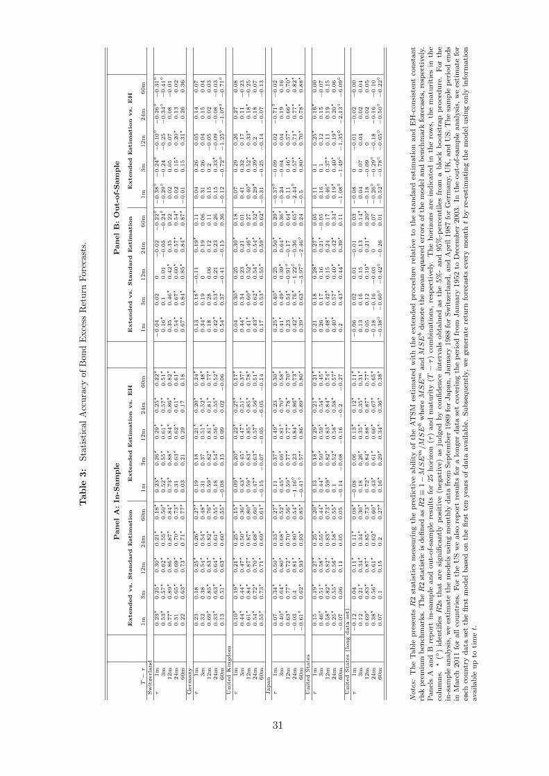
Tab

le3:

Sta

tist

ical

Acc

ura

cyof

Bon

dE

xce

ssR

etu

rnF

ore

cast

s.

PanelA:In

-Sam

ple

PanelB:Out-of-Sam

ple

Extended

vs.

Standard

Estim

atio

nExtended

Estim

atio

nvs.

EH

Extended

vs.

Standard

Estim

atio

nExtended

Estim

atio

nvs.

EH

T−τ

1m

3m

12m

24m

60m

1m

3m

12m

24m

60m

1m

3m

12m

24m

60m

1m

3m

12m

24m

60m

Switzerland

τ1m

0.23?

0.25?

0.30?

0.21?

0.18?

0.23?

0.26?

0.29?

0.25?

0.22?

−0.04

0.02

0−0.02−0.22◦−0.38◦−0.24◦−0.10◦−0.26◦−0.31◦

3m

0.53?

0.57?

0.62?

0.55?

0.50?

0.52?

0.55?

0.61?

0.57?

0.51?

0.16?

0.1

0.01−0.05−0.24◦−0.29◦−0.24−0.25−0.34◦−0.41◦

12m

0.77?

0.89?

0.86?

0.87?

0.84?

0.73?

0.88?

0.84?

0.86?

0.82?

0.35

0.46?

0.42?

0.35

0.22

0.02

0.05

0.07

0.08−0.01

24m

0.31

0.65?

0.69?

0.70?

0.73?

0.31

0.63?

0.62?

0.61?

0.61?

0.54?

0.67?

0.60?

0.57?

0.54?

0.02

0.15?

0.20?

0.13

0.02

60m

0.22

0.63?

0.73?

0.71?

0.77?

0.03

0.21

0.29

0.17

0.18

0.67?

0.84?

0.85?

0.84?

0.87?−0.01

0.15

0.31?

0.26

0.36

Germ

any

τ1m

0.23

0.18

0.25?

0.26?

0.27?

0.19

0.18

0.21?

0.20?

0.24?

0.13

0.18?−0.11

0.19?

0.11

0.04

0.26

0.05

0.14

0.07

3m

0.32

0.38

0.54?

0.54?

0.48?

0.31

0.37

0.51?

0.52?

0.48?

0.34?

0.19

00.19

0.06

0.31

0.26

0.04

0.15

0.04

12m

0.69?

0.85?

0.83?

0.82?

0.76?

0.59?

0.82?

0.81?

0.81?

0.77?

0.18

0.28

0.06

0.12

0.11

0.15

0.2

−0.05

0.02

0.03

24m

0.33?

0.63?

0.64?

0.61?

0.55?

0.18

0.54?

0.56?

0.55?

0.52?

0.42?

0.53?

0.21

0.23

0.26

0.15

0.33?−0.09−0.08−0.03

60m

0.13

0.51?

0.63?

0.60?

0.55?−0.08

0.15

0.09

0.02−0.06

0.54?

0.37−0.41−0.15

0.36−0.12−0.72◦−1.25◦−1.07◦−0.71◦

United

Kin

gdom

τ1m

0.10?

0.19?

0.21?

0.25?

0.15?

0.09?

0.20?

0.22?

0.27?

0.17?

0.04

0.30?

0.25

0.30?

0.18

0.07

0.29

0.26

0.27

0.08

3m

0.44?

0.44?

0.47?

0.50?

0.36?

0.43?

0.45?

0.47?

0.51?

0.37?

0.44?

0.34

0.23

0.21

0.01

0.41

0.32

0.17

0.11−0.23

12m

0.61?

0.84?

0.87?

0.87?

0.80?

0.59?

0.83?

0.85?

0.85?

0.78?

0.41?

0.60?

0.52?

0.46?

0.27

0.40?

0.52?

0.33?

0.18?−0.25

24m

0.54?

0.72?

0.70?

0.68?

0.60?

0.47?

0.63?

0.57?

0.56?

0.51?

0.43?

0.62?

0.54?

0.54?

0.52?

0.29?

0.39?

0.2

0.18

0.07

60m

0.55?

0.73?

0.71?

0.69?

0.61?−0.15−0.07−0.05−0.05−0.14

0.17

0.53?

0.55?

0.59?

0.62?−0.31−0.25−0.14−0.07−0.13

Japan

τ1m

0.07

0.34?

0.50?

0.33?

0.27?

0.11

0.37?

0.49?

0.23

0.30?

0.25?

0.40?

0.25

0.50?

0.29?−0.37◦−0.09

0.02−0.71◦−0.02

3m

0.40?

0.64?

0.80?

0.68?

0.52?

0.45?

0.66?

0.81?

0.70?

0.58?

0.41?

0.49?

0.39?

0.64?

0.36?−0.24−0.04

0.04

0.19

0.16

12m

0.63?

0.77?

0.72?

0.70?

0.56?

0.59?

0.77?

0.77?

0.78?

0.70?

0.23

0.54?−0.91◦−0.17

0.64?

0.11

0.46?

0.57?

0.66?

0.70?

24m

−0.03

0.4

0.81?

0.80?

0.54?−1.16◦

0.23

0.84?

0.86?

0.73?

0.42?

0.76?−1.22◦−0.36

0.65?−2.44◦

0.57?

0.71?

0.77?

0.82?

60m

−0.61◦

0.62?

0.93?

0.93?

0.85?−0.41◦

0.57?

0.86?

0.89?

0.80?

0.39?

0.63?−3.97◦−2.46◦

0.24−0.5

0.80?

0.70?

0.78?

0.88?

United

Sta

tes

τ1m

0.15

0.19?

0.27?

0.25?

0.20?

0.13

0.18?

0.29?

0.21?

0.21?

0.21

0.18

0.28?

0.27?

0.05

0.11

0.1

0.25?

0.16?

0.00

3m

0.46?

0.51?

0.58?

0.55?

0.44?

0.44?

0.50?

0.59?

0.54?

0.45?

0.26

0.17

0.16

0.21?−0.05

0.16

0.1

0.12

0.15−0.07

12m

0.58?

0.82?

0.82?

0.83?

0.73?

0.59?

0.82?

0.83?

0.84?

0.74?

0.48?

0.42?

0.15

0.24

0.17

0.46?

0.37?

0.11

0.19

0.15

24m

0.25?

0.55?

0.56?

0.58?

0.55?

0.1

0.52?

0.58?

0.58?

0.57?

0.40?

0.57?

0.40?

0.42?

0.34?

0.19?

0.40?

0.19?

0.20?

0.06

60m

−0.07

0.06

0.11

0.05

0.05−0.14−0.08−0.16−0.2

−0.27

0.2

0.43?

0.44?

0.39?

0.11−1.08◦−1.49◦−1.35◦−2.13◦−6.09◦

United

Sta

tes(long

data

set)

τ1m

−0.12

0.04

0.11?

0.11?

0.08?−0.08

0.06

0.13?

0.12?

0.11?

−0.06

0.02

0.01−0.01

0.03−0.08

0−0.01−0.02−0.00

3m

0.12

0.21?

0.34?

0.34?

0.30?

0.18

0.26?

0.35?

0.35?

0.31?

0.13

0.16

0.15

0.13

0.14?

0.04

0.07

0.04

0.02

0.04

12m

0.69?

0.83?

0.87?

0.85?

0.73?

0.72?

0.84?

0.88?

0.87?

0.77?

0.05

0.12

0.19?

0.21?

0.20?−0.18−0.09

00.02

0.05

24m

0.38?

0.56?

0.61?

0.62?

0.60?

0.43?

0.61?

0.66?

0.67?

0.65?

−0.18−0.16−0.03

00.07−0.26◦−0.29◦−0.18−0.16−0.10

60m

0.07

0.1

0.15

0.2

0.27?

0.16?

0.29?

0.34?

0.36?

0.38?

−0.38◦−0.60◦−0.42◦−0.26

0.01−0.52◦−0.78◦−0.65◦−0.50◦−0.22◦

Notes:

Th

eT

ab

lep

rese

ntsR

2st

ati

stic

sm

easu

rin

gth

ep

red

icti

ve

ab

ilit

yof

the

AT

SM

esti

mate

dw

ith

the

exte

nd

edp

roce

du

rere

lati

ve

toth

est

an

dard

esti

mati

on

an

dE

H-c

on

sist

ent

con

stant

risk

pre

miu

mb

ench

mark

s.T

heR

2st

ati

stic

isd

efin

edasR

2≡

1−MSEm/M

SEb

wh

ereMSEm

an

dMSEb

den

ote

the

mea

nsq

uare

der

rors

of

the

mod

elan

db

ench

mark

fore

cast

s,re

spec

tivel

y.P

an

els

Aan

dB

rep

ort

in-s

am

ple

an

dou

t-of-

sam

ple

resu

lts

for

25

hori

zon

(τ)

an

dm

atu

rity

(T−τ)

com

bin

ati

on

s,re

spec

tivel

y.T

he

hori

zon

sare

ind

icate

din

the

row

s,th

em

atu

riti

esin

the

colu

mn

s.?

(◦)

iden

tifi

esR

2s

that

are

sign

ifica

ntl

yp

osi

tive

(neg

ati

ve)

as

jud

ged

by

con

fid

ence

inte

rvals

ob

tain

edas

the

5%

-an

d95%

-per

centi

les

from

ab

lock

boots

trap

pro

ced

ure

.F

or

the

in-s

am

ple

an

aly

sis,

we

esti

mate

the

mod

els

usi

ng

month

lyd

ata

from

Sep

tem

ber

1989

for

Jap

an

,Janu

ary

1988

for

Sw

itze

rlan

d,

an

dA

pri

l1987

for

Ger

many,

UK

,an

dU

S.

Th

esa

mp

lep

erio

den

ds

inM

arc

h2011

for

all

cou

ntr

ies.

For

the

US

we

als

ore

port

resu

lts

for

alo

nger

data

set

cover

ing

the

per

iod

from

Janu

ary

1952

toD

ecem

ber

2003.

Inth

eou

t-of-

sam

ple

an

aly

sis,

we

esti

mate

for

each

cou

ntr

yd

ata

set

the

firs

tm

od

elb

ase

don

the

firs

tte

nyea

rsof

data

availab

le.

Su

bse

qu

entl

y,w

egen

erate

retu

rnfo

reca

sts

ever

ym

ontht

by

re-e

stim

ati

ng

the

mod

elu

sin

gon

lyin

form

ati

on

availab

leu

pto

tim

et.

31

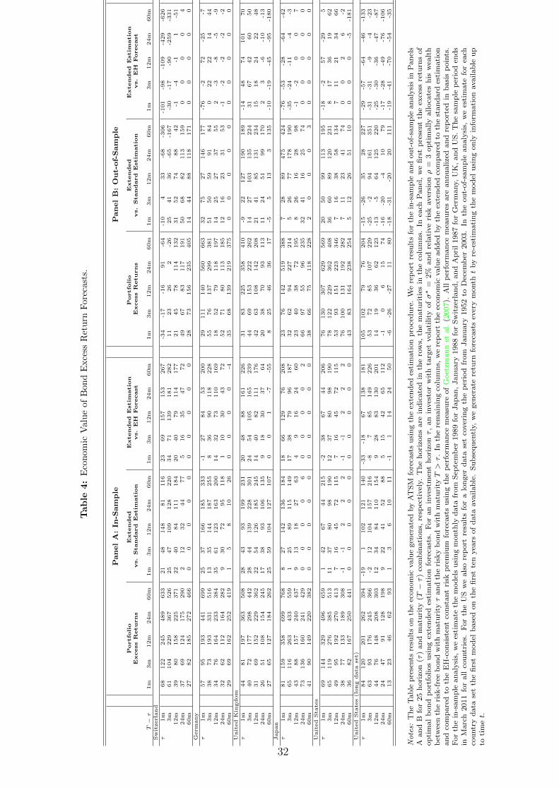
Tab

le4:

Eco

nom

icV

alu

eof

Bon

dE

xce

ssR

etu

rnF

ore

cast

s.

PanelA:In

-Sam

ple

PanelB:Out-of-Sam

ple

Portfo

lio

Extended

Extended

Estim

atio

nPortfo

lio

Extended

Extended

Estim

atio

nExcess

Returns

vs.

Standard

Estim

atio

nvs.

EH

Forecast

Excess

Returns

vs.

Standard

Estim

atio

nvs.

EH

Forecast

T−τ

1m

3m

12m

24m

60m

1m

3m

12m

24m

60m

1m

3m

12m

24m

60m

1m

3m

12m

24m

60m

1m

3m

12m

24m

60m

1m

3m

12m

24m

60m

Switzerland

τ1m

68

122

245

489

633

21

48

148

81

116

23

69

157

153

267

-34

-17

-16

91

-64

-10

433

-68

-306

-101

-98

-109

-429

-626

3m

61

104

229

367

526

25

47

109

128

220

34

71

139

181

282

11

23

26

2-2

625

41

36

-65

-167

-30

-17

-90

-259

-331

12m

39

80

158

225

371

22

40

84

111

184

20

40

79

114

177

21

45

78

114

132

31

52

74

88

42

-1-4

-11

-51

24m

37

69

124

175

290

212

32

44

77

516

35

47

72

49

67

83

117

191

50

68

82

113

159

00

00

460m

27

82

185

272

466

00

00

00

00

00

28

73

156

235

405

14

44

88

118

171

00

00

0Germ

any

τ1m

57

95

193

441

699

25

37

166

185

333

-127

84

53

200

29

111

140

560

663

32

75

27

146

177

-76

-272

-25

-73m

38

73

193

331

516

13

35

144

187

255

836

90

118

228

55

76

137

299

381

51

50

59

91

84

022

22

14

44

12m

34

76

164

233

384

35

61

123

163

200

14

32

73

110

169

18

52

79

118

197

14

25

27

37

55

2-3

-8-5

-924m

32

62

112

164

282

930

72

95

118

110

30

43

72

52

71

80

113

185

12

16

23

31

53

-1-2

-2-2

-260m

29

69

162

252

419

15

810

26

00

00

-435

68

139

219

375

00

00

00

00

00

United

Kin

gdom

τ1m

44

81

197

363

508

28

43

93

199

231

20

48

88

161

226

31

83

225

358

410

-922

127

190

189

-14

48

74

101

70

3m

40

72

177

298

442

28

44

139

228

301

24

54

105

165

239

44

69

153

222

262

14

27

103

135

224

31

67

42

60

50

12m

31

69

152

229

362

22

54

126

185

245

14

40

82

111

176

42

63

108

142

208

21

41

85

131

234

15

18

24

22

48

24m

26

51

108

154

245

17

38

93

106

135

918

30

37

64

20

38

70

93

113

11

24

51

99

170

23

-6-1

0-1

360m

27

65

127

184

262

25

59

104

127

107

00

1-7

-55

825

46

36

17

-55

13

3135

-10

-19

-45

-95

-180

Japan

τ1m

81

159

358

699

768

827

142

136

184

18

66

129

76

208

23

76

142

519

388

728

89

475

424

-76

-53

-28

-64

-42

3m

65

116

263

433

559

125

89

115

149

17

38

79

96

187

32

62

94

227

214

526

77

178

190

-35

-24

-11

-4-3

12m

43

88

157

240

437

913

18

27

63

49

16

24

60

23

40

38

72

195

826

16

28

98

-1-2

00

724m

73

136

160

241

429

00

00

60

00

02

66

97

55

96

235

32

41

16

25

74

00

00

060m

41

90

149

220

382

00

00

00

00

00

38

66

75

118

228

20

00

30

00

00

United

Sta

tes

τ1m

69

144

329

496

659

142

67

44

215

-238

67

44

206

76

130

307

629

569

20

50

99

113

195

-18

-257

-29

53m

65

119

276

385

513

11

37

80

98

190

12

37

80

98

190

78

122

229

362

408

36

60

89

120

231

817

36

19

62

12m

49

95

192

270

413

716

45

72

115

716

45

72

115

53

93

151

223

346

716

38

58

134

711

21

34

66

24m

38

77

133

189

308

-1-1

22

2-1

-12

22

76

100

131

192

282

711

23

41

74

00

26

-260m

36

82

167

250

441

00

00

00

00

00

43

83

164

238

254

512

26

51

10

00

0-5

-181

United

Sta

tes(long

data

set)

τ1m

84

120

201

262

394

-19

1102

121

140

-33

-18

67

138

181

105

102

79

76

204

-15

-26

35

28

227

-29

-57

-64

-46

-133

3m

63

93

176

245

366

-212

104

157

216

-87

85

149

226

53

72

85

107

229

-25

-294

161

351

-31

-31

-9-4

-23

12m

44

76

148

208

303

12

34

84

110

154

928

83

130

201

14

19

36

62

123

-13

-564

125

220

-25

-30

-36

-47

-87

24m

24

47

91

128

198

922

41

52

88

515

42

65

112

-10

615

74

-16

-20

-410

79

-17

-28

-49

-76

-106

60m

13

23

46

62

93

13

610

11

-11

14

24

50

-6-2

6-2

711

80

-18

-31

-20

20

111

-19

-41

-70

-54

-35

Notes:

Th

eT

ab

lep

rese

nts

resu

lts

on

the

econ

om

icvalu

egen

erate

dby

AT

SM

fore

cast

su

sin

gth

eex

ten

ded

esti

mati

on

pro

ced

ure

.W

ere

port

resu

lts

for

the

in-s

am

ple

an

dou

t-of-

sam

ple

an

aly

sis

inP

an

els

Aan

dB

for

25

hori

zon

(τ)

an

dm

atu

rity

(T−τ)

com

bin

ati

on

s,re

spec

tivel

y.T

he

hori

zon

sare

ind

icate

din

the

row

s,th

em

atu

riti

esin

the

colu

mn

s.In

each

Pan

el,

we

firs

tp

rese

nt

the

exce

ssre

turn

sof

op

tim

al

bon

dp

ort

folios

usi

ng

exte

nd

edes

tim

ati

on

fore

cast

s.F

or

an

inves

tmen

th

ori

zonτ,

an

inves

tor

wit

hta

rget

vola

tility

ofσ∗

=2%

an

dre

lati

ve

risk

aver

sionρ

=3

op

tim

ally

alloca

tes

his

wea

lth

bet

wee

nth

eri

sk-f

ree

bon

dw

ith

matu

rityτ

an

dth

eri

sky

bon

dw

ith

matu

rityT>τ.

Inth

ere

main

ing

colu

mn

s,w

ere

port

the

econ

om

icvalu

ead

ded

by

the

exte

nd

edco

mp

are

dto

the

stan

dard

esti

mati

on

an

dco

mp

are

dto

the

EH

-con

sist

ent

con

stant

risk

pre

miu

mfo

reca

sts

usi

ng

the

per

form

an

cem

easu

reof

Goet

zman

net

al.

(2007).

All

per

form

an

cem

easu

res

are

an

nu

alize

dan

dre

port

edin

basi

sp

oin

ts.

For

the

in-s

am

ple

an

aly

sis,

we

esti

mate

the

mod

els

usi

ng

month

lyd

ata

from

Sep

tem

ber

1989

for

Jap

an

,Janu

ary

1988

for

Sw

itze

rlan

d,

an

dA

pri

l1987

for

Ger

many,

UK

,an

dU

S.

Th

esa

mp

lep

erio

den

ds

inM

arc

h2011

for

all

cou

ntr

ies.

For

the

US

we

als

ore

port

resu

lts

for

alo

nger

data

set

cover

ing

the

per

iod

from

Janu

ary

1952

toD

ecem

ber

2003.

Inth

eou

t-of-

sam

ple

an

aly

sis,

we

esti

mate

for

each

cou

ntr

yd

ata

set

the

firs

tm

od

elb

ase

don

the

firs

tte

nyea

rsof

data

availab

le.

Su

bse

qu

entl

y,w

egen

erate

retu

rnfo

reca

sts

ever

ym

ontht

by

re-e

stim

ati

ng

the

mod

elu

sin

gon

lyin

form

ati

on

availab

leu

pto

tim

et.

32

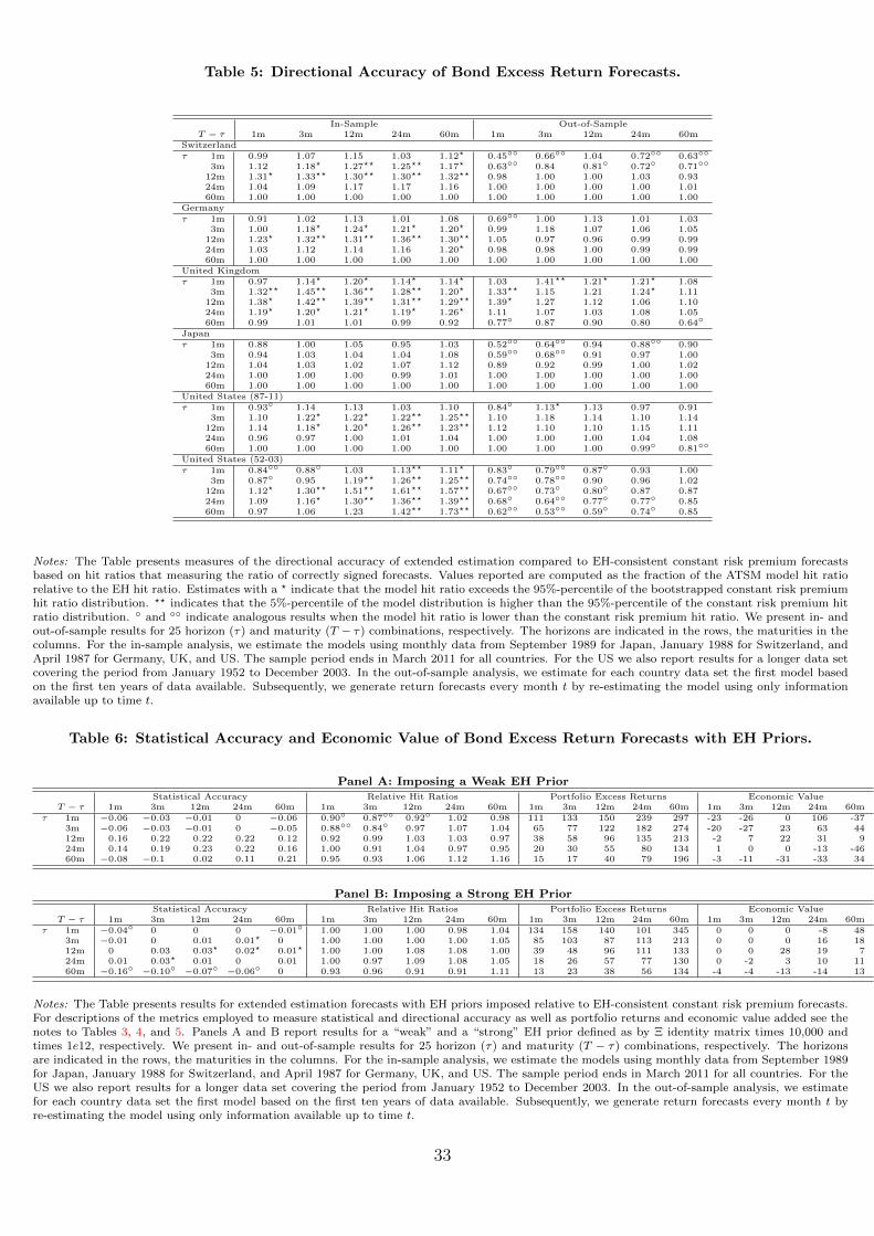
Table 5: Directional Accuracy of Bond Excess Return Forecasts.

In-Sample Out-of-SampleT − τ 1m 3m 12m 24m 60m 1m 3m 12m 24m 60m

Switzerlandτ 1m 0.99 1.07 1.15 1.03 1.12? 0.45◦◦ 0.66◦◦ 1.04 0.72◦◦ 0.63◦◦

3m 1.12 1.18? 1.27?? 1.25?? 1.17? 0.63◦◦ 0.84 0.81◦ 0.72◦ 0.71◦◦

12m 1.31? 1.33?? 1.30?? 1.30?? 1.32?? 0.98 1.00 1.00 1.03 0.9324m 1.04 1.09 1.17 1.17 1.16 1.00 1.00 1.00 1.00 1.0160m 1.00 1.00 1.00 1.00 1.00 1.00 1.00 1.00 1.00 1.00

Germanyτ 1m 0.91 1.02 1.13 1.01 1.08 0.69◦◦ 1.00 1.13 1.01 1.03

3m 1.00 1.18? 1.24? 1.21? 1.20? 0.99 1.18 1.07 1.06 1.0512m 1.23? 1.32?? 1.31?? 1.36?? 1.30?? 1.05 0.97 0.96 0.99 0.9924m 1.03 1.12 1.14 1.16 1.20? 0.98 0.98 1.00 0.99 0.9960m 1.00 1.00 1.00 1.00 1.00 1.00 1.00 1.00 1.00 1.00

United Kingdomτ 1m 0.97 1.14? 1.20? 1.14? 1.14? 1.03 1.41?? 1.21? 1.21? 1.08

3m 1.32?? 1.45?? 1.36?? 1.28?? 1.20? 1.33?? 1.15 1.21 1.24? 1.1112m 1.38? 1.42?? 1.39?? 1.31?? 1.29?? 1.39? 1.27 1.12 1.06 1.1024m 1.19? 1.20? 1.21? 1.19? 1.26? 1.11 1.07 1.03 1.08 1.0560m 0.99 1.01 1.01 0.99 0.92 0.77◦ 0.87 0.90 0.80 0.64◦

Japanτ 1m 0.88 1.00 1.05 0.95 1.03 0.52◦◦ 0.64◦◦ 0.94 0.88◦◦ 0.90

3m 0.94 1.03 1.04 1.04 1.08 0.59◦◦ 0.68◦◦ 0.91 0.97 1.0012m 1.04 1.03 1.02 1.07 1.12 0.89 0.92 0.99 1.00 1.0224m 1.00 1.00 1.00 0.99 1.01 1.00 1.00 1.00 1.00 1.0060m 1.00 1.00 1.00 1.00 1.00 1.00 1.00 1.00 1.00 1.00

United States (87-11)τ 1m 0.93◦ 1.14 1.13 1.03 1.10 0.84◦ 1.13? 1.13 0.97 0.91

3m 1.10 1.22? 1.22? 1.22?? 1.25?? 1.10 1.18 1.14 1.10 1.1412m 1.14 1.18? 1.20? 1.26?? 1.23?? 1.12 1.10 1.10 1.15 1.1124m 0.96 0.97 1.00 1.01 1.04 1.00 1.00 1.00 1.04 1.0860m 1.00 1.00 1.00 1.00 1.00 1.00 1.00 1.00 0.99◦ 0.81◦◦

United States (52-03)τ 1m 0.84◦◦ 0.88◦ 1.03 1.13?? 1.11? 0.83◦ 0.79◦◦ 0.87◦ 0.93 1.00

3m 0.87◦ 0.95 1.19?? 1.26?? 1.25?? 0.74◦◦ 0.78◦◦ 0.90 0.96 1.0212m 1.12? 1.30?? 1.51?? 1.61?? 1.57?? 0.67◦◦ 0.73◦ 0.80◦ 0.87 0.8724m 1.09 1.16? 1.30?? 1.36?? 1.39?? 0.68◦ 0.64◦◦ 0.77◦ 0.77◦ 0.8560m 0.97 1.06 1.23 1.42?? 1.73?? 0.62◦◦ 0.53◦◦ 0.59◦ 0.74◦ 0.85

Notes: The Table presents measures of the directional accuracy of extended estimation compared to EH-consistent constant risk premium forecastsbased on hit ratios that measuring the ratio of correctly signed forecasts. Values reported are computed as the fraction of the ATSM model hit ratiorelative to the EH hit ratio. Estimates with a ? indicate that the model hit ratio exceeds the 95%-percentile of the bootstrapped constant risk premiumhit ratio distribution. ?? indicates that the 5%-percentile of the model distribution is higher than the 95%-percentile of the constant risk premium hitratio distribution. ◦ and ◦◦ indicate analogous results when the model hit ratio is lower than the constant risk premium hit ratio. We present in- andout-of-sample results for 25 horizon (τ) and maturity (T − τ) combinations, respectively. The horizons are indicated in the rows, the maturities in thecolumns. For the in-sample analysis, we estimate the models using monthly data from September 1989 for Japan, January 1988 for Switzerland, andApril 1987 for Germany, UK, and US. The sample period ends in March 2011 for all countries. For the US we also report results for a longer data setcovering the period from January 1952 to December 2003. In the out-of-sample analysis, we estimate for each country data set the first model basedon the first ten years of data available. Subsequently, we generate return forecasts every month t by re-estimating the model using only informationavailable up to time t.

Table 6: Statistical Accuracy and Economic Value of Bond Excess Return Forecasts with EH Priors.

Panel A: Imposing a Weak EH PriorStatistical Accuracy Relative Hit Ratios Portfolio Excess Returns Economic Value

T − τ 1m 3m 12m 24m 60m 1m 3m 12m 24m 60m 1m 3m 12m 24m 60m 1m 3m 12m 24m 60mτ 1m −0.06 −0.03 −0.01 0 −0.06 0.90◦ 0.87◦◦ 0.92◦ 1.02 0.98 111 133 150 239 297 -23 -26 0 106 -37

3m −0.06 −0.03 −0.01 0 −0.05 0.88◦◦ 0.84◦ 0.97 1.07 1.04 65 77 122 182 274 -20 -27 23 63 4412m 0.16 0.22 0.22 0.22 0.12 0.92 0.99 1.03 1.03 0.97 38 58 96 135 213 -2 7 22 31 924m 0.14 0.19 0.23 0.22 0.16 1.00 0.91 1.04 0.97 0.95 20 30 55 80 134 1 0 0 -13 -4660m −0.08 −0.1 0.02 0.11 0.21 0.95 0.93 1.06 1.12 1.16 15 17 40 79 196 -3 -11 -31 -33 34

Panel B: Imposing a Strong EH PriorStatistical Accuracy Relative Hit Ratios Portfolio Excess Returns Economic Value

T − τ 1m 3m 12m 24m 60m 1m 3m 12m 24m 60m 1m 3m 12m 24m 60m 1m 3m 12m 24m 60mτ 1m −0.04◦ 0 0 0 −0.01◦ 1.00 1.00 1.00 0.98 1.04 134 158 140 101 345 0 0 0 -8 48

3m −0.01 0 0.01 0.01? 0 1.00 1.00 1.00 1.00 1.05 85 103 87 113 213 0 0 0 16 1812m 0 0.03 0.03? 0.02? 0.01? 1.00 1.00 1.08 1.08 1.00 39 48 96 111 133 0 0 28 19 724m 0.01 0.03? 0.01 0 0.01 1.00 0.97 1.09 1.08 1.05 18 26 57 77 130 0 -2 3 10 1160m −0.16◦ −0.10◦ −0.07◦ −0.06◦ 0 0.93 0.96 0.91 0.91 1.11 13 23 38 56 134 -4 -4 -13 -14 13

Notes: The Table presents results for extended estimation forecasts with EH priors imposed relative to EH-consistent constant risk premium forecasts.For descriptions of the metrics employed to measure statistical and directional accuracy as well as portfolio returns and economic value added see thenotes to Tables 3, 4, and 5. Panels A and B report results for a “weak” and a “strong” EH prior defined as by Ξ identity matrix times 10,000 andtimes 1e12, respectively. We present in- and out-of-sample results for 25 horizon (τ) and maturity (T − τ) combinations, respectively. The horizonsare indicated in the rows, the maturities in the columns. For the in-sample analysis, we estimate the models using monthly data from September 1989for Japan, January 1988 for Switzerland, and April 1987 for Germany, UK, and US. The sample period ends in March 2011 for all countries. For theUS we also report results for a longer data set covering the period from January 1952 to December 2003. In the out-of-sample analysis, we estimatefor each country data set the first model based on the first ten years of data available. Subsequently, we generate return forecasts every month t byre-estimating the model using only information available up to time t.

33

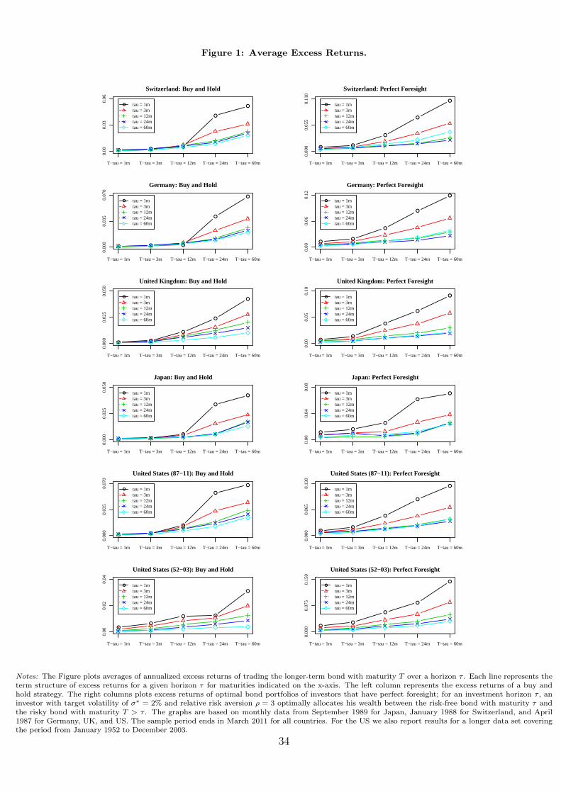
Figure 1: Average Excess Returns.

● ●●

●

●

Switzerland: Buy and Hold

T−tau = 1m T−tau = 3m T−tau = 12m T−tau = 24m T−tau = 60m

0.00

0.03

0.06

● tau = 1mtau = 3mtau = 12mtau = 24mtau = 60m

● ●

●

●

●

Switzerland: Perfect Foresight

T−tau = 1m T−tau = 3m T−tau = 12m T−tau = 24m T−tau = 60m

0.00

00.

055

0.11

0

● tau = 1mtau = 3mtau = 12mtau = 24mtau = 60m

● ● ●

●

●

Germany: Buy and Hold

T−tau = 1m T−tau = 3m T−tau = 12m T−tau = 24m T−tau = 60m

0.00

00.

035

0.07

0

● tau = 1mtau = 3mtau = 12mtau = 24mtau = 60m

●●

●

●

●

Germany: Perfect Foresight

T−tau = 1m T−tau = 3m T−tau = 12m T−tau = 24m T−tau = 60m

0.00

0.06

0.12

● tau = 1mtau = 3mtau = 12mtau = 24mtau = 60m

● ●

●

●

●

United Kingdom: Buy and Hold

T−tau = 1m T−tau = 3m T−tau = 12m T−tau = 24m T−tau = 60m

0.00

00.

025

0.05

0

● tau = 1mtau = 3mtau = 12mtau = 24mtau = 60m

●●

●

●

●

United Kingdom: Perfect Foresight

T−tau = 1m T−tau = 3m T−tau = 12m T−tau = 24m T−tau = 60m

0.00

0.05

0.10

● tau = 1mtau = 3mtau = 12mtau = 24mtau = 60m

● ●●

●

●

Japan: Buy and Hold

T−tau = 1m T−tau = 3m T−tau = 12m T−tau = 24m T−tau = 60m

0.00

00.

025

0.05

0

● tau = 1mtau = 3mtau = 12mtau = 24mtau = 60m

●●

●

●

●

Japan: Perfect Foresight

T−tau = 1m T−tau = 3m T−tau = 12m T−tau = 24m T−tau = 60m

0.00

0.04

0.08

● tau = 1mtau = 3mtau = 12mtau = 24mtau = 60m

● ●

●

●

●

United States (87−11): Buy and Hold

T−tau = 1m T−tau = 3m T−tau = 12m T−tau = 24m T−tau = 60m

0.00

00.

035

0.07

0

● tau = 1mtau = 3mtau = 12mtau = 24mtau = 60m

●●

●

●

●

United States (87−11): Perfect Foresight

T−tau = 1m T−tau = 3m T−tau = 12m T−tau = 24m T−tau = 60m

0.00

00.

065

0.13

0

● tau = 1mtau = 3mtau = 12mtau = 24mtau = 60m

●●

● ●

●

United States (52−03): Buy and Hold

T−tau = 1m T−tau = 3m T−tau = 12m T−tau = 24m T−tau = 60m

0.00

0.02

0.04

● tau = 1mtau = 3mtau = 12mtau = 24mtau = 60m

●●

●

●

●

United States (52−03): Perfect Foresight

T−tau = 1m T−tau = 3m T−tau = 12m T−tau = 24m T−tau = 60m

0.00

00.

075

0.15

0

● tau = 1mtau = 3mtau = 12mtau = 24mtau = 60m

Notes: The Figure plots averages of annualized excess returns of trading the longer-term bond with maturity T over a horizon τ . Each line represents theterm structure of excess returns for a given horizon τ for maturities indicated on the x-axis. The left column represents the excess returns of a buy andhold strategy. The right columns plots excess returns of optimal bond portfolios of investors that have perfect foresight; for an investment horizon τ , aninvestor with target volatility of σ∗ = 2% and relative risk aversion ρ = 3 optimally allocates his wealth between the risk-free bond with maturity τ andthe risky bond with maturity T > τ . The graphs are based on monthly data from September 1989 for Japan, January 1988 for Switzerland, and April1987 for Germany, UK, and US. The sample period ends in March 2011 for all countries. For the US we also report results for a longer data set coveringthe period from January 1952 to December 2003.

34

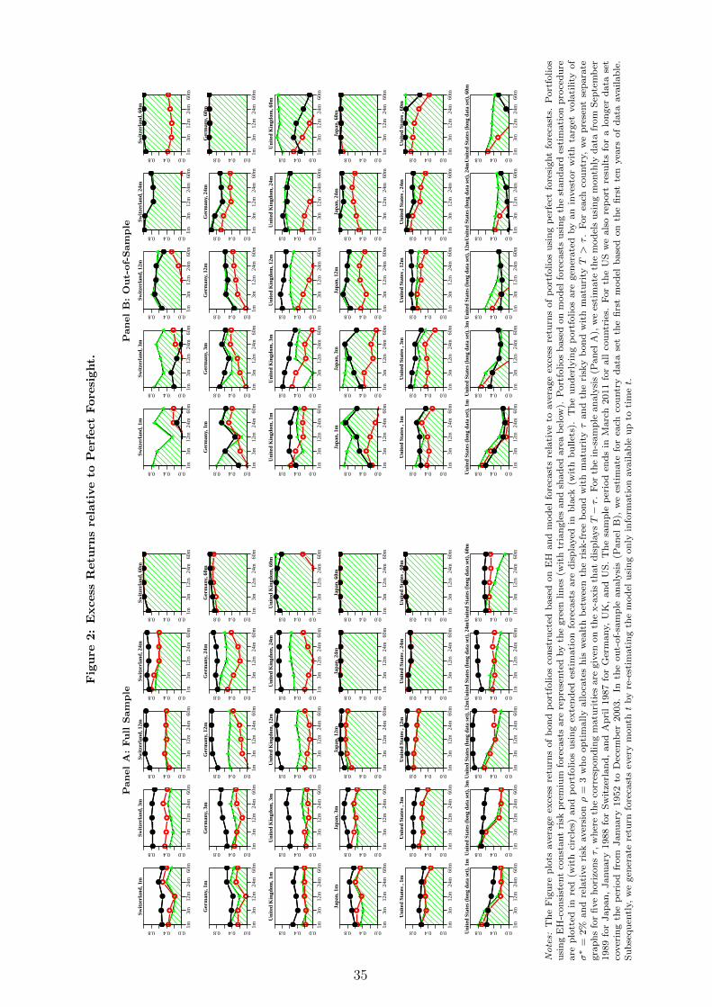
Fig

ure

2:

Excess

Retu

rns

rela

tive

toP

erf

ect

Fore

sight.

PanelA:Full

Sam

ple

●●

●

●●

●●

●●

●

1m3m

12m

24m

60m

0.00.40.8

Sw

itzer

land

, 1m

●●

●●

●

●●

●●

●

1m3m

12m

24m

60m

0.00.40.8

Sw

itzer

land

, 3m

●●

●●

●

●●

●●

●

1m3m

12m

24m

60m

0.00.40.8

Sw

itzer

land

, 12m

●●

●●

●

●●

●●

●

1m3m

12m

24m

60m

0.00.40.8

Sw

itzer

land

, 24m

●●

●●

●●

●●

●●

1m3m

12m

24m

60m

0.00.40.8

Sw

itzer

land

, 60m

●●

●

●●

●●

●

●●

1m3m

12m

24m

60m

0.00.40.8

Ger

man

y, 1

m

●●

●●

●

●●

●●

●

1m3m

12m

24m

60m

0.00.40.8

Ger

man

y, 3

m

●

●●

●

●

●●

●●

●

1m3m

12m

24m

60m

0.00.40.8

Ger

man

y, 1

2m

●

●

●●

●

●●

●●

●

1m3m

12m

24m

60m

0.00.40.8

Ger

man

y, 2

4m

●●

●●

●●

●●

●●

1m3m

12m

24m

60m

0.00.40.8

Ger

man

y, 6

0m

●●

●●

●

●●

●●

●

1m3m

12m

24m

60m

0.00.40.8

Uni

ted

Kin

gdom

, 1m

●●

●●

●

●●

●●

●

1m3m

12m

24m

60m

0.00.40.8

Uni

ted

Kin

gdom

, 3m

●●

●●

●

●●

●●

●

1m3m

12m

24m

60m

0.00.40.8

Uni

ted

Kin

gdom

, 12m

●●

●

●●

●●

●●

●

1m3m

12m

24m

60m

0.00.40.8

Uni

ted

Kin

gdom

, 24m

●●

●●

●

●●

●●

●

1m3m

12m

24m

60m

0.00.40.8

Uni

ted

Kin

gdom

, 60m

●●

●

●●

●●

●●

●

1m3m

12m

24m

60m

0.00.40.8

Japa

n, 1

m

●●

●●

●

●●

●●

●

1m3m

12m

24m

60m

0.00.40.8

Japa

n, 3

m

●●

●●

●●

●●

●●

1m3m

12m

24m

60m

0.00.40.8

Japa

n, 1

2m●

●●

●●

●●

●●

●

1m3m

12m

24m

60m

0.00.40.8

Japa

n, 2

4m●

●●

●●

●●

●●

●

1m3m

12m

24m

60m

0.00.40.8

Japa

n, 6

0m

●●

●●

●

●●

●●

●

1m3m

12m

24m

60m

0.00.40.8

Uni

ted

Sta

tes

, 1m

●●

●●

●

●●

●●

●

1m3m

12m

24m

60m

0.00.40.8

Uni

ted

Sta

tes

, 3m

●●

●●

●

●●

●●

●

1m3m

12m

24m

60m

0.00.40.8

Uni

ted

Sta

tes

, 12m

●●

●●

●●

●●

●●

1m3m

12m

24m

60m

0.00.40.8

Uni

ted

Sta

tes

, 24m

●●

●●

●●

●●

●●

1m3m

12m

24m

60m

0.00.40.8

Uni

ted

Sta

tes

, 60m

●

●

●●

●

●●

●●

●

1m3m

12m

24m

60m

0.00.40.8Uni

ted

Sta

tes

(long

dat

a se

t), 1

m

●●

●●

●

●●

●●

●

1m3m

12m

24m

60m

0.00.40.8Uni

ted

Sta

tes

(long

dat

a se

t), 3

m

●

●●

●●

●●

●●

●

1m3m

12m

24m

60m

0.00.40.8

Uni

ted

Sta

tes

(long

dat

a se

t), 1

2m

●●

●●

●

●●

●●

●

1m3m

12m

24m

60m

0.00.40.8

Uni

ted

Sta

tes

(long

dat

a se

t), 2

4m

●●

●●

●●

●●

●●

1m3m

12m

24m

60m

0.00.40.8

Uni

ted

Sta

tes

(long

dat

a se

t), 6

0m

PanelB:Out-of-Sam

ple

●●

●

●●

●

●●

●

●1m

3m12

m24

m60

m

0.00.40.8

Sw

itzer

land

, 1m

●●

●

●●

●●

●●

●1m

3m12

m24

m60

m

0.00.40.8

Sw

itzer

land

, 3m

●●

●●

●

●

●●

●

●

1m3m

12m

24m

60m

0.00.40.8

Sw

itzer

land

, 12m

●●

●●

●

●●

●●

●

1m3m

12m

24m

60m

0.00.40.8

Sw

itzer

land

, 24m

●●

●●

●

●●

●●

●

1m3m

12m

24m

60m

0.00.40.8

Sw

itzer

land

, 60m

●

●●

●●

●

●

●

●●

1m3m

12m

24m

60m

0.00.40.8

Ger

man

y, 1

m

●

●●

●●

●●

●

●●

1m3m

12m

24m

60m

0.00.40.8

Ger

man

y, 3

m

●

●●

●●

●

●●

●●

1m3m

12m

24m

60m

0.00.40.8

Ger

man

y, 1

2m

●●

●●

●

●●

●●

●

1m3m

12m

24m

60m

0.00.40.8

Ger

man

y, 2

4m●

●●

●●

●●

●●

●

1m3m

12m

24m

60m

0.00.40.8

Ger

man

y, 6

0m

●●

●●

●

●

●●

●●

1m3m

12m

24m

60m

0.00.40.8

Uni

ted

Kin

gdom

, 1m

●●

●●

●

●●

●●

●

1m3m

12m

24m

60m

0.00.40.8

Uni

ted

Kin

gdom

, 3m

●●

●●

●

●●

●●

●

1m3m

12m

24m

60m

0.00.40.8

Uni

ted

Kin

gdom

, 12m

●●

●

●

●

●●

●●

●

1m3m

12m

24m

60m

0.00.40.8

Uni

ted

Kin

gdom

, 24m

●

●

●

●

●

●

●●

●

●

1m3m

12m

24m

60m

0.00.40.8

Uni

ted

Kin

gdom

, 60m

●

●●

●●

●

●●

●

●

1m3m

12m

24m

60m

0.00.40.8

Japa

n, 1

m

●●

●●

●

●

●●

●

●

1m3m

12m

24m

60m

0.00.40.8

Japa

n, 3

m

●●

●●

●

●

●●

●●

1m3m

12m

24m

60m

0.00.40.8

Japa

n, 1

2m

●●

●●

●

●●

●●

●

1m3m

12m

24m

60m

0.00.40.8

Japa

n, 2

4m●

●●

●●

●●

●●

●

1m3m

12m

24m

60m

0.00.40.8

Japa

n, 6

0m

●●

●●

●

●●

●●

●

1m3m

12m

24m

60m

0.00.40.8

Uni

ted

Sta

tes

, 1m

●●

●●

●

●●

●●

●

1m3m

12m

24m

60m

0.00.40.8

Uni

ted

Sta

tes

, 3m

●●

●●

●

●●

●●

●

1m3m

12m

24m

60m

0.00.40.8

Uni

ted

Sta

tes

, 12m

●●

●●

●

●●

●●

●

1m3m

12m

24m

60m

0.00.40.8

Uni

ted

Sta

tes

, 24m

●●

●●

●

●●

●●

●

1m3m

12m

24m

60m

0.00.40.8

Uni

ted

Sta

tes

, 60m

●

●

●●

●

●

●

●●

●

1m3m

12m

24m

60m

0.00.40.8Uni

ted

Sta

tes

(long

dat

a se

t), 1

m

●

●

●●

●

●●

●●

●

1m3m

12m

24m

60m

0.00.40.8Uni

ted

Sta

tes

(long

dat

a se

t), 3

m

●

●

●●

●

●●

●●

●

1m3m

12m

24m

60m

0.00.40.8

Uni

ted

Sta

tes

(long

dat

a se

t), 1

2m

●●

●●

●

●●

●●

●

1m3m

12m

24m

60m

0.00.40.8

Uni

ted

Sta

tes

(long

dat

a se

t), 2

4m

●

●

●

●

●

●

●

●

●

●

1m3m

12m

24m

60m

0.00.40.8

Uni

ted

Sta

tes

(long

dat

a se

t), 6

0m

Notes:

Th

eF

igu

rep

lots

aver

age

exce

ssre

turn

sof

bon

dp

ort

folios

con

stru

cted

base

don

EH

an

dm

od

elfo

reca

sts

rela

tive

toaver

age

exce

ssre

turn

sof

port

folios

usi

ng

per

fect

fore

sight

fore

cast

s.P

ort

folios

usi

ng

EH

-con

sist

ent

con

stant

risk

pre

miu

mfo

reca

sts

are

rep

rese

nte

dby

the

gre

enli

nes

(wit

htr

ian

gle

san

dsh

ad

edare

ab

elow

).P

ort

folios

base

don

mod

elfo

reca

sts

usi

ng

the

stan

dard

esti

mati

on

pro

ced

ure

are

plo

tted

inre

d(w

ith

circ

les)

an

dp

ort

folios

usi

ng

exte

nd

edes

tim

ati

on

fore

cast

sare

dis

pla

yed

inbla

ck(w

ith

bu

llet

s).

Th

eu

nd

erly

ing

port

foli

os

are

gen

erate

dby

an

inves

tor

wit

hta

rget

vola

tility

of

σ∗

=2%

an

dre

lati

ve

risk

aver

sionρ

=3

wh

oop

tim

ally

alloca

tes

his

wea

lth

bet

wee

nth

eri

sk-f

ree

bon

dw

ith

matu

rityτ

an

dth

eri

sky

bon

dw

ith

matu

rityT>τ.

For

each

cou

ntr

y,w

ep

rese

nt

sep

ara

tegra

ph

sfo

rfi

ve

hori

zon

sτ,

wh

ere

the

corr

esp

on

din

gm

atu

riti

esare

giv

enon

the

x-a

xis

that

dis

pla

ysT−τ.

For

the

in-s

am

ple

an

aly

sis

(Pan

elA

),w

ees

tim

ate

the

mod

els

usi

ng

month

lyd

ata

from

Sep

tem

ber

1989

for

Jap

an

,Janu

ary

1988

for

Sw

itze

rlan

d,

an

dA

pri

l1987

for

Ger

many,

UK

,an

dU

S.

Th

esa

mp

lep

erio

den

ds

inM

arc

h2011

for

all

cou

ntr

ies.

For

the

US

we

als

ore

port

resu

lts

for

alo

nger

data

set

cover

ing

the

per

iod

from

Janu

ary

1952

toD

ecem

ber

2003.

Inth

eou

t-of-

sam

ple

an

aly

sis

(Pan

elB

),w

ees

tim

ate

for

each

cou

ntr

yd

ata

set

the

firs

tm

od

elb

ase

don

the

firs

tte

nyea

rsof

data

availab

le.

Su

bse

qu

entl

y,w

egen

erate

retu

rnfo

reca

sts

ever

ym

ontht

by

re-e

stim

ati

ng

the

mod

elu

sin

gon

lyin

form

ati

on

availab

leu

pto

tim

et.

35

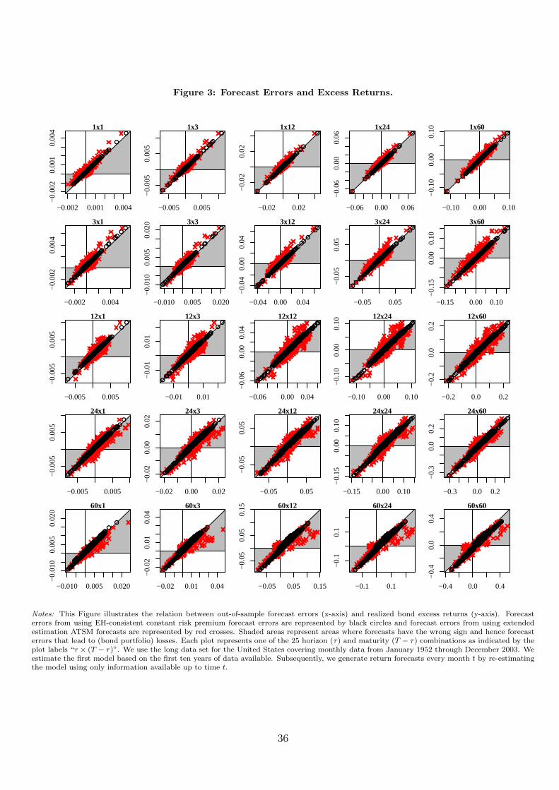
Figure 3: Forecast Errors and Excess Returns.

−0.002 0.001 0.004

−0.

002

0.00

10.

004 1x1

Forecast Error ( = Realized − Model)

●●●●●●●●●●●●●●

●●●●●●●●●●●●●●●●●●●●●●●●●●●●●●●●●●●●

●●●●●●●●●

●●●●●

●●●●●●

●●●●●●

●●●●●●

●●●

●●

●●●●

●●●●

●●

●

●●

●●●●●

●●

●●

●●●●●

●

●●●

●●

●●

●●●

●

●●●●●●●

●

●

●●●

●

●

●●●●●

●

●

●

●●

●

●

●

●●

●

●●●●

●●●●

●

●●●●●●

●

●●●●●●

●●

●●●●

●●●●●

●●●●●

●●●

●

●●●

●●●

●●●●

●●

●●

●

●●●

●●

●

●

●●

●

●●

●

●

●●

●

●

●

●

●●

●●

●

●

●

●

●

●●

●

●

●

●

●●●●●

●

●

●●●●●●●●●●●●●●●

●●

●●●

●●●●●●●●●●

●●

●●●

●●

●●●

●●●●●●●●

●●●●●

●●●

●●

●●●●●

●●

●●●

●●●●●

●●●

●●

●

●●●

●●●●●●●●●

●●●

●●●●●●●●●●

●●●●

●●●

●●

●●●●●●●●●●●●●●●●●●●●

●●●●●

●

●●●●●●●●●●●●

●●●

●●●●●●●

●●●●●

●●●

●●●●●●●

●●●

●●●●●●

●●●●●●●●●●●●●●●●●●●

●

●●●

●●●●

●

●●●●●●●

●●●●●●●●●●●●●●●●●●●●●●

●●●●●●

−0.005 0.005

−0.

005

0.00

5

1x3

Forecast Error ( = Realized − Model)

Rea

lized

exc

ess

retu

rn

●●●●●●●●●●●●●●●

●●●●●●●●●●●●●●●●●●●●●●●●●●●●●●●●●●●●●●●●●●●●●

●●●●

●●●●●●

●●

●●●●●●●●

●●

●●●●●

●●●

●●

●●●

●

●●

●

●●

●●●●

●

●●●

●●●●

●

●

●●

●●●

●●

●●●

●

●●

●●●●●

●

●

●●●●

●

●●●

●●

●

●

●●

●

●

●

●

●●

●

●●●

●

●●●●

●

●●●

●●●

●

●●●●●●

●●

●●●●●

●●●●●●●●●●●●

●

●●

●●●

●●●●●

●

●●●

●

●

●

●

●

●

●

●

●●

●●

●●

●●●

●

●

●●

●●

●

●●

●●

●

●

●●

●

●●

●

●●

●●

●

●

●

●●●●

●●

●●●●●

●●●●●●

●●●

●●

●●●●

●●●●●●●

●

●●

●●●

●

●●●●●●●●●●●●●

●

●●●

●●●●●

●●●●●●●

●●●

●●

●●

●●●●●●●●●●●●●●●

●●●●●●●●●●●●●

●●●●

●●●

●●

●●●●●●●●●●●●●●●●●●●●●●

●●●●●●●

●●●●●●●●●●●●●●●●●●●●●●●●●●●●●●●

●●●●●●●●●●●

●●●●●●●●●●●●●

●●●●●●●●●

●●●●●●

●●●●●●●●

●●●●●●●●●●●●●●●●●●●●●●●●●●●●

−0.02 0.02

−0.

020.

02

1x12

Forecast Error ( = Realized − Model)R

ealiz

ed e

xces

s re

turn

●●●●●●●●●●●●●●●●●●●

●●●●●●●●●●●●●●●●●●●●●●●●●●●

●●

●●●●●●

●

●●●●●

●●

●●

●

●●●●●●●

●●●●●●●●●●

●

●●●●

●●

●●●

●

●●●

●

●

●

●●●●●●

●

●●●

●

●●

●

●

●

●●

●●●●

●

●●

●

●●●

●●●●●●

●●●

●

●●●

●●

●●

●●

●●●

●

●

●●●●

●●

●

●

●●●●

●

●

●●

●●●

●

●●●●●●

●

●

●●●●●●●●●

●●●●●●●●●●

●●

●●

●

●●●●●

●●●

●

●

●●

●

●

●

●

●

●

●

●●●

●

●●

●

●

●●

●

●

●

●●

●

●●●

●●

●

●●●●

●●

●●

●

●

●●

●

●●

●●●●

●●●

●

●●

●●

●●●●

●

●●●

●●

●●●●●●●●

●●

●●●

●●●

●●●●●●●

●●●

●

●●●

●●●●●

●●●●

●●●

●●●●●

●

●●

●●

●●●●●●

●●●●●●●●●●●●●●●●●●●

●●●●●●●●●

●●●●●●●

●●

●●●●●●●●●●●●

●●●●

●●

●●●●

●●●●●●●●●

●●●●●●●●●●●●●●●●●●

●●●

●●●

●●●●●●●●●

●●●●

●●●●●●●●●●●●●●●

●●●●●●

●●

●●●●●

●●●●

●●●●●

●●●●

●●●●●

●●●●●●●●●

●●●

−0.06 0.00 0.06

−0.

060.

000.

06

1x24

Forecast Error ( = Realized − Model)

Rea

lized

exc

ess

retu

rn

●●●

●●●

●●●●●●●●●●●●●●●●●●●●●●●●●●●●●●●●●●●●●●●●

●●●●●●●●

●

●●

●●●

●

●

●●●

●●●●●●

●●●●●●●●●●●

●

●●

●●

●●

●●●

●

●●●

●●

●

●●●●●

●

●

●

●●●

●

●

●

●

●

●●

●●

●●

●

●●●

●●●●●

●●●●●

●●

●

●●

●●●●●

●

●

●●●●

●●●

●●●

●●

●

●●●●

●

●

●●●

●●

●

●●●●●●

●

●

●●●●●●●●●

●●●●●●●●●●●

●

●●

●

●●●●●

●●

●

●

●

●●

●

●

●

●

●

●

●

●●●

●

●●

●

●

●●

●●

●

●●

●

●●

●

●●

●

●●●

●

●●●

●

●

●

●●

●

●

●

●●●●

●●●

●

●●

●●

●●●●

●

●●

●

●●

●●●●●

●●●

●●

●●

●

●

●●●

●●●●●

●●

●●

●

●●●

●●●●

●●●

●●

●●

●●●

●●●●

●

●●

●●●●●●

●●●

●●●●●●●●●●●●●●●●●

●●●

●●●●●●

●●

●●●●●

●

●●

●●●●●●

●●●●●

●●●●●●

●●●●

●

●●●●●●●●

●●●●

●●●●●●

●●●●●●●●

●●●

●●●

●●●●●●●●

●●

●●●

●●●●●●●●●●●

●●●●●●●●●●●●●●●●●●●

●●

●●●●

●

●●●

●

●●

●●

●●●●●●●

●●

●

●●

●

−0.10 0.00 0.10

−0.

100.

000.

10 1x60

Forecast Error ( = Realized − Model)

Rea

lized

exc

ess

retu

rn

●●●●●●●●●●●

●●●●●●●●●●●●●●●●●●●●●●●●●●●●●●●●●●●

●●

●

●●●●●

●

●

●●

●●

●

●

●●

●

●●●●●●

●●●●●●●

●●●●

●

●

●

●●●●●

●

●

●

●●

●

●

●

●

●●●●●●

●

●●●●

●

●

●

●

●

●●

●

●

●

●

●

●●●

●●●●●

●●●●●●●

●

●●

●

●●

●●

●●

●●●●

●●●●●

●

●●

●

●●●

●

●

●

●

●●●●

●

●●●

●●

●

●

●

●●●●●

●

●●

●

●●●●●●●●●●

●●

●

●

●

●

●●

●●

●●●

●

●●

●

●

●

●

●

●

●

●

●

●●

●

●

●

●

●

●

●

●●

●

●●

●

●●

●

●

●

●

●●●●

●●

●

●

●

●

●●

●

●

●

●●

●

●

●●●

●

●

●

●●

●

●●●

●

●●

●

●●

●●

●●

●

●

●●

●

●

●

●

●

●

●●●●●●

●

●●

●●

●

●

●●

●

●

●●●

●

●●

●●

●●

●

●●

●●●●

●

●

●●

●●

●●●

●●●

●

●●●●●●●●●●

●●●

●●

●

●

●●

●●●●

●●

●●

●●●

●●●●●●

●●●

●●

●●●●●

●

●●

●●●

●●

●●

●

●●

●●●●●●

●●●●

●●●

●●●

●●●

●

●●●●

●

●●●

●●

●●●●●●

●●

●●●●

●

●●●

●●●●

●●●●●

●

●●

●●●●●

●●●●●●

●●

●●

●●

●●●

●

●

●●●

●●●

●●

●

●

●●●

●

●●

●

●

●●●

−0.002 0.004

−0.

002

0.00

4

3x1

Forecast Error ( = Realized − Model)

●●●●●●●●●●●●

●●●

●●●●●●●●●●●●●●●●●●●●●●●●●●●●●●●●●●●●●●●●

●●●●●●●●●●●●●●●●●

●●●●●●●●

●●●

●●●●●●●

●●●●

●●●●●

●●●●

●●●

●●●

●●●

●●

●●

●●●●●●●●

●●●●●

●●●●●●

●●

●●●●

●●

●●

●●

●

●

●●

●●

●●●

●●●●

●●

●●●

●●●●●●●●●●●●●

●●●

●●●●●●●●●●●●●●●

●●●●

●●●●●●●●

●●

●●

●●

●●

●

●

●

●

●

●●

●

●●

●

●

●

●●

●

●

●

●

●●

●

●●

●

●●

●●

●

●

●●

●●

●●

●●

●●●

●●●●●●●●●

●●●

●●●

●●

●●

●●●

●●●●●●●●●●

●●●

●●●

●●●

●●●

●●●●

●●

●

●●●

●●●●●●●●●

●●

●●●

●●●●

●●

●

●●●●●●

●●●●●●●●

●●●●●●●●●●●

●●

●●●●●●

●●●●●●●●●●●●●●●●●●●●●●●●●

●●●●●●●●●●●●●●●●●●●●●●●●●●●●●●●●●●●●●●●●●●●●●●

●●●

●●●●●●●●●●●●●●●●●

●●●●●●●●

●●●●●●●●●●●

●●●●●●●●●●●●●●●●●●●●●●●●●

−0.010 0.005 0.020

−0.

010

0.00

50.

020 3x3

Forecast Error ( = Realized − Model)

Rea

lized

exc

ess

retu

rn

●●●●●●●●●●●●●●●

●●●●●●●●●●●●●●●●●●●●●●●●●●●●●●●●●●●●●●●●

●●●●●●●●●●●●●●●

●●

●●●●●●

●●●●●

●●●●

●●

●●●●●

●●

●●●

●●●●●●●●●

●●

●●

●●

●●

●●●●●●●●

●●●●●●●

●●●●

●●

●●●●●

●

●●

●

●●

●

●

●

●●●

●●

●●●●

●●

●●●

●●●●●●●

●●●●●●●●

●●●●●●●●●●●●●●●●●●

●●●●●●●●●●

●●

●●●

●

●●

●

●

●

●

●

●●●

●●

●●

●●●

●●

●

●

●

●

●

●●

●

●

●

●●

●

●

●●

●●

●●

●●

●●

●●●

●●●●●●●●

●●●

●●●

●●

●

●●●

●●●●●●●●●●●●

●●●

●●●●●●●●●●

●

●●●●●●●

●●●●●●●●●●●●●

●●●

●●●●●●●●●●

●●●●●●●●●●●●●●●●●●●●

●●●●●●●●●●

●●●●●●●●●●●●●●●●●●●●●●●●●

●●●●●●●●●●●●●●●●●●●●●●●●●●●●●●●●●●●●●●●●●●●●●●●●●●●●●●●●●●●●●●●●●●●●●●●

●●●●●●●●●●●

●●●●●●

●●●●●●●●●●●●●●●●●●●

−0.04 0.00 0.04

−0.

040.

000.

04

3x12

Forecast Error ( = Realized − Model)

Rea

lized

exc

ess

retu

rn

●●●●●●●●●●●●●●●●●●●●●●●●

●●●●●●●●●●●●●●●●●●●●●●●●●●●●

●●●

●●●●●●●

●●●●●●●●●●

●●●

●●●●●

●●●

●●●

●●●

●●●●●

●●

●●●

●●●●

●●●

●●

●●

●

●

●

●●

●●●●

●●●●●

●●●●●

●●

●●●●

●●

●

●●

●●●

●●●

●●

●

●●

●●●●

●

●●

●●

●●

●●●

●●●●●●●

●●●●●●

●●●●●●●●●●

●●●●●●●●●●●●●

●●●

●●●●

●●

●

●●

●

●●

●

●●

●

●

●●

●

●●

●●

●●

●●

●●

●

●

●

●

●

●●

●

●

●●

●●●●

●●

●●

●●

●●

●●●

●●●●

●●

●●

●●●

●●●

●●●

●●●

●●●●●●●●●

●●●

●●●

●●●●●●●●●●

●

●●●●●●

●●●●●●

●●●●●●

●●

●●

●●●

●●●●●●●●

●●●●●

●●●●●●●●●

●●●●●●

●●●

●●●●●

●●●

●●●●●●

●●●●●●●●

●●●

●●●●●●

●

●●●●●●

●●●●●●

●●●●●

●●●●●●●●●●●●●●●●●●●●●●●●●●●●●

●●●●●●●●●●●●●●●●●●●●●●●●●

●●●●●●●●

●●●●

●●●●●

●●●●●●●●●●●●●●●●●●●

−0.05 0.05

−0.

050.

05

3x24

Forecast Error ( = Realized − Model)R

ealiz

ed e

xces

s re

turn

●●●●●●●●●●●●●●●●●●●●●●●●●●●●●●●●●●●●●●●●●●●●

●●●●●●●●

●●●

●●●●●●●

●●●●

●●●●●●

●●●

●●●●●

●●●

●●●

●●●●

●●●●

●●

●●●

●●●●

●●

●●●

●●

●

●

●

●●

●●●●

●●●●●

●●●●●

●●●

●●●

●●

●

●●

●●●

●●●

●●●

●●

●●●●●

●●●●

●●

●●●

●●●●●●

●●●●●●

●●●

●●●●●●●●●●●●●●●●●●

●●●

●●●

●●

●●

●●

●

●●

●

●●

●

●●

●

●●●

●

●●●

●

●

●●●

●●

●

●

●

●

●

●●●

●

●●

●●●●

●●

●●

●●

●●

●●●

●●●●

●●

●●

●●●

●●●

●●●

●●●

●●●●

●●●●●●●●

●

●●●●●●●

●●

●●●

●●

●●●●●

●●

●●●●●

●●●●●●

●

●●

●●●

●●

●●●●●

●●

●●●●●●●●●●●●●

●●●●●

●

●●●

●●●●

●●●

●●●●

●●●

●●●●●●●

●●●

●●●●●

●●●

●●●●●●●●●●

●●●

●●

●●●●

●●●

●●●●●●

●●●●●●●●●●●●●●

●●●

●●●●●●●●●●●●●●●●●●●●

●●●●●●

●●●●●●●●

●●●

●●

●●

●●

●●●●

●●●●●

●●●●●●●●●●

−0.15 0.00 0.10

−0.

150.

000.

10

3x60

Forecast Error ( = Realized − Model)

Rea

lized

exc

ess

retu

rn

●●●●●●●●●●●●●●●●●●●●●●●●●

●●●●●●●●●●●●●●●●●●●●●●

●●●●●

●

●●

●●●●●●●

●

●●

●●●●

●●●●●

●●●●

●●

●●●

●●●

●●●

●●●●

●

●

●

●●●

●●●●

●●●●

●

●●

●

●

●

●●

●●

●●

●

●●●●●●●●●●

●●●●●

●●

●●

●●●●

●●●

●●●

●●

●●●●

●●

●●

●●●

●●

●

●●

●●●●●

●●●●●

●

●●

●●●●●●●●●●●●●●●●

●●

●●●

●

●●

●

●●●

●●

●

●●

●

●●

●

●●

●

●●●

●

●●

●●

●

●

●●

●●

●

●

●

●

●

●●

●

●●

●

●●

●●

●

●

●

●

●●

●●

●

●●

●●

●●

●

●●

●

●●●●●●

●●●

●●

●

●●

●●

●●

●●●

●●●

●

●●

●●

●●●

●●●

●●

●

●●

●●●

●

●

●

●●●●●●

●●●●●

●

●●

●

●●

●●

●●●●

●●

●

●●●

●●●

●●●●●●

●

●●●●

●●

●

●●

●●●●

●●●

●

●●

●●

●●●●●

●●●

●

●●

●●

●●●

●●

●●

●●●●●

●

●●●●●●

●●

●●●●●●

●●

●●

●●●●

●●

●●●

●●●●●

●●●●●

●●

●

●●

●●●●●●●●●●

●●●

●●●●●●

●●●●●●

●●

●●

●●

●●●

●●

●●

●●

●●●

●●

●●●

●

●

●●●

●

●

●●●

●

−0.005 0.005

−0.

005

0.00

5

12x1

Forecast Error ( = Realized − Model)

●●●●

●●●●●●●●●●●●●●●●●●●●●●●●●●●●●●●●●●●●●●●●●●●●●●●

●●●

●

●●

●●●●●●●●●●●

●●●●

●●●●●

●●●●●●

●●

●●●

●●●

●●●●

●●●●●●●●●

●●●

●●●●

●●●

●

●●●●●●●●●

●●●●

●●●●●●●●●●

●●

●●●●●●●●●●

●●●

●●●

●●●

●●●●●

●●

●●●●●●●●●●●●●●●●

●●●●●

●●●●●●●●●●●●

●●●●●

●●●

●●●●

●●

●

●

●

●

●

●

●

●

●●●

●●

●●

●

●

●

●●●

●

●●

●●●●

●●●

●

●

●●●

●●●●●●●●●●●●

●●●●

●●●

●●●●●●●●●●●●

●●●●

●●

●●●●

●●●●●●●●●●●

●●●●●●●●●●

●●

●●

●●●●●●

●●●●●●●●

●●●

●●●●●●●

●●●●●●●●●●●●●●●●●●●●

●●●

●●●●●●●●●●●●●●

●●●●●●●●●●●●●●●●

●●●●●

●●●●●●●●●●●●●●●●●●●●●●●●●●●●

●●●●●●●●●●●●●●●●●●●●●●●

●●

●●●●●●

●●●●●●

●●●●●●●●●●●●●●

●●●

●●●●●●●

●●●●●●

−0.01 0.01

−0.

010.

01

12x3

Forecast Error ( = Realized − Model)

Rea

lized

exc

ess

retu

rn

●●●●●●●●●●●●●●●●●●●●●●●●●●●●●●●●●●●●●●●●●●●●●●●●●●●●

●●●●

●●●

●●●●●●

●●●●●●●●●●●●●

●●●●●

●●●●●●

●●●●

●●

●●●●●●●

●●

●●●

●●●

●

●●●●

●●●●●●●●●●●●●

●●●●●●

●●●

●●

●

●●●●

●●●●●

●●●●●

●●●

●●●

●●●●

●●

●●●●●●●●●●●●●●●●●●●●●●●●●●●●●

●●●●

●●●●●●

●●

●

●●●

●●●

●●●

●

●

●

●●●

●

●

●

●

●●

●

●

●●●

●

●●

●

●●●●●●

●●

●●●

●●●●●●●

●●●●●●●●●●●

●

●●●●●

●●●●●

●●●●

●●●●●●●●

●●●

●●●●●●●●●●●●●●●●

●●●

●●●●●

●●●●●●●●●●●●

●●●●●●●

●●●●

●●●●●●●●●●●●●●

●●●●●●●●

●●●●●●●●●●●

●●●●

●●●●●●●●●●●●

●●●●●●

●●●●●

●●●●●●●●●●●●●●●●●●●●●●●●●●●●●●●●●●●●●●●

●●●●●●●●●

●●●●●●●●

●●●●●●●●●●●●●●●●●●●●

●●●●●●

●●●●●●●●●●

−0.06 0.00 0.04

−0.

060.

000.

04

12x12

Forecast Error ( = Realized − Model)

Rea

lized

exc

ess

retu

rn

●●●●●●●●●●●●●●●●●●●●●●●●●●●●●●●●●●●

●●●●●●●●●●●●

●●●●●●●●●

●●●●●

●●●●

●●●●●●●●●

●●●

●●●●●

●●●

●●●●

●●●●

●

●

●●●●●●

●●●

●●

●●

●●

●

●●●●

●●●●●●●●●●●

●●●

●●

●●●

●●●●

●

●●

●●●

●●●●●●●

●●

●●

●●

●●

●

●●●●

●●

●●

●●●●●●

●●●

●●●

●●●●●●●●●

●●●

●●●●●

●●●●

●●●●

●●

●

●●●

●●●

●

●●

●●

●●●●

●●

●

●

●●●

●

●●●

●

●●

●

●

●●●●●

●●

●●●

●●●●●●●●●

●●●●

●●●●●

●

●●

●●●●

●●●●●●

●●●●●●●

●●●●●●●

●●●

●●●●●●

●●●●●●

●●●

●●●

●●●

●●●●

●●●●●●●●●

●●●●●

●●●

●●

●●●●●●●●●●●●●

●●●●

●●●●

●●●●

●●●●●●●

●●

●●●●●●●●●●●

●●

●●●●●●

●●●●●●

●●●●●●●●●●●

●●●●●●●●●●●●●●●

●●●●●●●●●●●●●

●●●●●●●●●●●●●●●

●●

●●●●●●●●●●●●●●

●●●●●●

●●●

●●●●

●●●●●●●

●●

−0.10 0.00 0.10

−0.

100.

000.

10

12x24

Forecast Error ( = Realized − Model)

Rea

lized

exc

ess

retu

rn

●●●●●●●●●●●●●●●●●●●●●●●●●●●●●●●●●●●

●●●●●●●●●

●●●

●●●●●●●●●

●●●●●●

●●●●●

●●●●●●●

●●●

●●●●●●●●

●●●●

●●●

●●

●●●●●●●

●●●

●●

●●●●

●

●●●●

●●●●●●●●●●●●

●●●●●

●●

●●●●

●

●●●●●

●●●●●●●

●●●

●●●

●●

●

●●●●

●●

●●●●●●●●

●●●●

●●●●●●●

●●●●●●●

●●●●●

●●●●

●●●

●

●●

●

●●●

●●

●

●

●●

●●

●●●

●●●

●

●

●●

●●

●●●

●

●

●●

●

●●●●●●

●

●●●

●●●●

●●●

●●

●●●

●●

●●●●

●

●●

●●●●●●●

●●●

●●

●●●●●

●●●

●●●

●●●●●●●●●●

●●●●●●

●●

●●

●●●

●●●

●●●

●●●●●

●●●●

●●●●●

●●●●

●●●●●●●

●●●●●●●●●●

●●●

●●●●

●●●●●●●●●

●●

●●●●●●●●●●

●●

●●●●●

●●

●●●●●

●

●●●●●●●●●●●●●●

●●●●●

●●●●●●●●

●●●●●●●●●●●●●

●●●●●●●●●●

●●●●●

●●●●●●●●●

●●●

●●●●

●●●●●●●●

●●●●

●●●

●●●●●

●

−0.2 0.0 0.2

−0.

20.

00.

2

12x60

Forecast Error ( = Realized − Model)R

ealiz

ed e

xces

s re

turn

●●●●●●●●●●●●●●●●●●●●●●●●●●●●●●●●●●●

●●●●●●●●●

●●●

●●●●●●●

●●●●●

●●●●●●

●●●●●●

●●●●●

●●●●

●●●●●

●●●

●●●●

●●

●●●●●●●

●●●●●

●●●●●

●●●●

●●●●●●●●●●●●

●●●●●●●

●●●●

●●

●●●●●

●●●●●●●

●●

●●●●

●●

●●●●

●●

●●

●●●●●●●●●

●●●

●●●●●●●●●●●●●●●●

●●

●●●

●●●

●

●●

●●●●

●●●

●●●

●●

●●●●●●

●

●

●●

●●

●●●

●

●

●●

●

●●●

●●●●

●

●●

●●●

●

●●●

●●

●●●

●●●●●

●●

●●

●●●●●●

●

●●●

●●

●●●●●

●●

●

●●

●●●

●●●●●●●●

●●●●●

●●●

●●

●●

●●●

●●

●●

●●●●●

●●●●●●●●

●●●●

●●

●●

●●●●●●●●●

●●●●●

●●

●

●●●●

●●●●●

●●●●

●●

●●●●

●●●●●●

●●

●

●●●●

●●●●●

●●

●

●●●●●●●

●●●●●●●

●●●●●

●●●●●●●

●

●●●●●●●●●

●●●●

●●●●●●●●

●●●

●●●●

●●●

●●●●●●

●●

●●●●

●

●●●●●

●●●

●●●●

●●●

●

●●●●

●

−0.005 0.005

−0.

005

0.00

5

24x1

Forecast Error ( = Realized − Model)

●●●

●●●●●●●

●●

●●●●●●●●●●●●●●●●●●●●●●●●●●●●●●●●●●●●●●

●●●

●●●●

●

●●

●

●●

●●

●●●

●●●

●●●

●●●●●●●●

●●●●

●●

●●

●

●

●●●

●●●

●●

●

●

●●●●

●●●●

●

●●●●●●

●●

●●●●●●●

●●

●●●

●●

●●●●●●●

●●

●

●●●

●●●

●●●

●●

●

●●●●

●●●

●●●

●●●●●●●

●●●

●●●

●●

●●●●

●●

●●●●●

●●

●●

●

●●●●

●●

●●

●●●●

●

●

●

●●

●

●

●

●

●●●●

●

●

●●

●

●

●

●

●

●

●●●

●

●

●

●

●●●

●●

●●●●

●●

●●●●●

●●●●●

●●●●●●

●

●●

●

●●

●●

●

●●

●●

●●●●●●●●●●

●●●●

●●

●●●●

●●●

●●●●●●

●●

●●●

●●●●

●●●

●

●

●●

●●●●●●●●●

●●●●●●●●●●●

●●●

●

●●

●●

●●

●●

●●●●●●●

●●

●●●

●●

●●●

●●●●

●

●

●●●●●●●

●

●

●●●

●●●●

●●●●

●●●

●●●●●

●●●

●●

●●●●●●●

●●●

●●

●●●●●●●●●●

●●●●

●●●●

●

●●●●●●●●●●

●●●●●●●

●●●

●●●●●●

●

●●

●

●●●

●●●

●●

−0.02 0.00 0.02

−0.

020.

000.

02

24x3

Forecast Error ( = Realized − Model)

Rea

lized

exc

ess

retu

rn

●●●●●●●●●●●●●●●●●

●●●●●●●●●●●●●●●●●●●●●●●●●●●●●●●●

●●●●●●●●

●●●●●●●●●

●●●●●●●●●●●●●●●●

●●●

●●●●●

●

●●●●●●●●●

●●●●●●

●●●●●

●●●●●

●●●

●●●●

●●●

●●

●

●●●●

●●●●●●

●●

●●●●●●●●

●●●●●●

●●●●

●●●●●●

●●●●●●●●●●●●

●●●●●●●

●●●●●●●●●

●●

●

●●●●

●●

●●●

●●

●●

●●

●●

●●●

●

●●

●●●

●

●●

●●

●

●

●●

●●●

●●

●●

●●●

●●●●●●●●●●●●●

●●●●

●●●●●●●●

●●

●●

●●●

●●●●●●●

●●●●●●●●

●●●●●

●●●●●

●●●●●●●

●●●●

●●●●●

●●●●●●●

●●

●●●●●●●●●●●●●●●●●●●●●●●

●●●●●●●●●

●●●●●●●●●

●●●●

●●●●

●●●●

●

●

●●●●●●●●

●●●●●●●●

●●●●●●●●●●●●●●●

●●●●●●●●●●●●●●

●●●●●●●●●●●●●●●●●●

●●●

●●●●

●●●●●●●

●●●●●●●●●●●●●●

●●●●●●

●●●

●●

−0.05 0.05

−0.

050.

05

24x12

Forecast Error ( = Realized − Model)

Rea

lized

exc

ess

retu

rn

●●●●●●●●●●●●●●●●●●●●●●●●●●●●●●●●●●●

●●●●●●

●●●●●●●●●●●●●●●

●●●●●●●●●●●●●●●●●

●●●●●●●●●

●●●

●●●●

●●●●●●

●●●●

●●●●●●●

●●●●

●●●●

●●

●●●●●●

●●●●●

●●●●

●●●●

●●●●●●

●●●

●●●●●●●●●●●●●●●●●●●●●

●●●●●●●●●●●●●

●●●●●●●●●●●

●●●●

●●

●

●●●

●●●

●

●●●

●

●●●●●●

●●

●●

●●

●●●

●

●●

●●●●

●●

●●●●●

●●

●●●

●●●●

●●●●●●●●

●●●●●●●

●●●●●●

●●

●●●●●●●●●

●●

●●●●●

●●●●●●●●●

●●

●●●

●●●●●●●

●●●●●●●

●●●●●●●●●●

●●●●

●●●●●

●●●●●●●●

●●●●●●●

●●●●●●●●●●●●●●

●●●●●●●●

●●●●●●●●●●●●●●●●●●

●●●●●●●●

●●●●●●

●●●●●●●●●●●●●●●●●●

●●●●●●●●

●●●●●●●●●●●●●●●●●●

●●●●

●●●●●

●●●●●●●●●●●●●●●●●●●●●●●●

●●●

−0.15 0.00 0.10

−0.

150.

000.

10

24x24

Forecast Error ( = Realized − Model)

Rea

lized

exc

ess

retu

rn

●●●●●●●●●●●●●●●●●●●●●●●●●●●●●●●●●

●●●●●

●●●●●●●●●●●●●●●●●●●●●

●●●●●●●●●●●●

●●●●●●●●●●●

●●●●●

●●●●

●●●●

●●●

●●●●●●●●

●●●●

●●●●

●●

●●●●●●●●●●●●●●

●●●

●●●

●●●●●

●●●●●

●●

●●●●●●●●●●●●●●●●●

●●●●●●●●●●●●●

●●●●●●●●●

●●

●●●●

●●

●

●●●

●●●

●

●●●●

●●●●●●

●●

●●

●●●●

●

●

●●

●●●●

●●

●

●●●●

●●

●●●●●

●●●●

●●●●●●

●●●

●●●●

●●●●●●

●●●●

●●

●●●●●●●

●

●●●

●●●●

●●

●●●●

●●●

●●●●●●●

●●

●●

●●●●●

●●●●●●●●●●

●●●●●●●

●●●●●●

●●●●●●●●

●●●

●●●●●●●●●●●●●●

●●●●

●●●●●●●●●●●●●●●●●●●●●●

●●●●●●●●●●●

●●●●●

●●●●●●●●●●

●●●●●●

●●●●●●●●

●●●●●●●●●●●●●●●●●●●

●●●●●●●

●●●●●●

●●●●

●●●●●●●●●●●●●●●●●

●

−0.3 0.0 0.2

−0.

30.

00.

2

24x60

Forecast Error ( = Realized − Model)

Rea

lized

exc

ess

retu

rn

●●●●●●●●●●●●●●●●●●●●●●●●●●●●●●●●●●●

●●●●●●●●●●●●●●

●●●●●

●●●●●●●●●●●●●●●●●

●●●●●●●●●●●

●●●●●

●●●●

●●●●

●●●●

●●●●●●●●●●●

●●●●●●●●●●●●

●●●●●●●●●●●●●

●●●●●●●●●●●●

●●●●●●●

●●●●●●●●●●●

●●

●●●●●●●●●●●●●●●●●●●●●●

●●●●

●●

●●●●

●●●●

●●●●●●●

●●●

●

●

●●

●●●●

●

●

●●

●●●●

●●●

●●●

●●

●

●●●

●●●

●●●●

●●●●●

●●●

●●●●●

●●●●

●●●●●

●●●●●●●●

●●

●●●●●●●

●●

●●●●●●

●●●

●●●●●

●●●

●●

●●●●●●●●●●●●●●●●●●●●●

●●●●●●

●●●●●●●●●●●

●●●●●●●●●●●●●

●●

●●●●●●●●●●●●●●●●●●●●●●●●●●

●●●●●●●●●●●●●

●●●

●●●●●●●●

●●●●●●●

●●●●●●●●●●●●●●●●

●●●●●●●●●

●●●●●●●

●●●●●●●●

●●●●

●●●●

●●●●●●●●

●●●

●●●

−0.010 0.005 0.020

−0.

010

0.00

50.

020 60x1

●●●

●●●●●●●●

●●●●●●●●●●●●●●●●●●●●●●●●●●

●●●●●●●●●●

●●

●●●●

●●

●

●●●●

●●

●●

●●

●●

●●●●

●●●●

●●●●

●●●●●

●

●●●

●●

●

●●

●

●

●●

●●

●

●

●

●●●●●

●

●●●●●●

●●

●●

●●●

●

●●●

●●●●●

●●

●●●

●

●

●

●

●●

●●●●

●●●●●●

●●

●

●

●●●●

●●●

●●●●●

●●

●●●●●●●●

●●

●●●●

●●

●●●

●●

●●●●●

●●●

●●

●

●●

●●●

●●●

●

●

●●

●

●●

●●

●●

●●

●●

●

●

●

●●●●

●●●

●●

●●●●●

●●●

●●

●●●●●●●●●●●●●

●●

●●

●●

●●

●●●●

●

●●

●●●

●

●●●

●●●●●

●●

●●●

●●

●

●●●

●●

●●

●

●

●●

●

●●

●●●●

●●●●●●

●

●

●●

●●●

●

●●●●●

●●●●●●

●●●●●●

●●●

●●●

●

●●●●●●

●●

●●●●●

●●●●

●●

●●

●●●●

●

●

●●●●●●●

●

●

●●●

●●

●●

●●●●●●●●●●●

●

●

●

●

●●●●●●●●●●●●●

●●●●

●●●●●●

●●●●●●●●

●

●

●●

−0.02 0.01 0.04

−0.

020.

010.

04

60x3

Rea

lized

exc

ess

retu

rn

●●●●●●●●●●●

●●●●●●●●●●●●●●●●●●●●●●●●●●

●●●●●●●●●●●

●●●●●●

●●

●●●●●●

●●●●

●●

●●●●

●●●●●●●●●●●●●

●

●●●●●

●

●●●●

●●●●

●

●●

●●●●●●●●●

●●●●●●●

●●●

●●●●

●●●●●●●●●●●

●●

●

●●●●●●●●

●●●●●

●●●●

●●

●●●●

●●

●●●●●●

●●●●●●●

●●

●●●●

●●

●●●●●●●●●●●●

●●

●●

●●●●●●●●●

●

●●●

●●●

●●●●●

●●

●

●

●

●●●●●●●

●●

●●●●●

●●●●

●●●●●●●●●●●●●●

●●●●●●

●●●●●

●●●●

●●●

●●

●●●

●●●●●

●

●●●●

●●

●●●

●●

●●●

●●●

●●

●●●●●

●●●●●●

●

●●●●●●●●●●●●●●

●●●●●●●●●●●●●●●●

●●●●●●●

●●

●●●●●●●●●●●

●●

●●●●

●

●

●●●●●●●

●

●

●●●

●●●●

●●●●●●●●●●●●

●●

●●

●●●●●●●●●●●●●●●●

●●●●●●●●●●●●●●●

●

●●

−0.05 0.05 0.15

−0.

050.

050.

15 60x12

Rea

lized

exc

ess

retu

rn

●●●●●●●●●●●●●●●●●●●●●●●●●●●●●

●●●●●●●●●●

●●●●●●●

●●●●●●●

●●●

●●●●●●●●●●●●●●●●●●●●●●

●●●●●●●●

●●●●●●

●●●●●●●●

●●●●●●●●●●●●●●●●●●●●●●●●●●●●●●●●●●●●●●●●●●●

●●●●●●●●●

●●

●●●

●●

●

●●●●●

●●●●●●●●●●●●●

●

●●●●●●

●

●●●

●●●●●●●●●

●●●●●●●●●●

●●●

●●

●●●

●●●●●●●●●●

●●

●●●●●●●

●●●●●●●●●●●●

●●●●●

●●●●●●●●●●●●●●●●●●●●●●●●●●●●●●

●●●●●●

●●●●●

●●●●●●●●●●

●●●●●●●●●●●●●●●●

●●●●●●●●

●●●●●●●●●●●●●●●●●●●●●●●●●●●●●●●●●●●●●●●●●●●●●●●●●

●●

●●●●●●●

●●●●●

●●●●●●●●●●

●●●●●●●●●●●●●●●

●●●●●●●●●●●●●●●●●●●●●●●●●●●

●●

−0.1 0.1

−0.

10.

1

60x24

Rea

lized

exc

ess

retu

rn

●●●●●●●●●●●●●●●●●●●●●●●

●●●●●●●●●●●●●●●●

●●●●●●●

●●●●●●●

●●●●●●●●●●●●●●●●●●●●●●●●●

●●●●●●●●

●●●●●●●●●

●●●●●●

●●●●●●●●●●●●●●●●●●●●●●●●●●●●●●●●●●●●●●●●●●●●●●●

●●●●●

●●●●

●●

●●●●

●●●●●●

●●●●●

●●●

●●

●●●●●●

●

●●●

●●●●●●●●●

●●●●●●●●●●

●●●●●

●●●●●●●

●●●●●●●

●●●●●●

●●●●●

●●●●●●●●●

●●●●●

●●●●●●●●●●●●●●●●

●●●●●●●●●●

●●●●●

●●●●●●●

●●●

●●●●●●

●●●●●●●

●●●

●●●●●●●●●●●●●●●●●●

●●●●●●●●●●●●

●●●●●●●●●●●●●●●●●●●●●●●●●●●●●●●●●●●●●

●●●●●●●●●●●

●●●●●●●●●●●●●

●●●●●●●●●●●

●●●●●●●●●●●●●●●●●●●●●●●●●●●●●●●●●

−0.4 0.0 0.4

−0.

40.

00.

4

60x60

Rea

lized

exc

ess

retu

rn

●●●●●●●●●●●●●●●●●●●●●●●●●●●●●●●●●●●●●

●●●●●●●

●●●●●

●●●●●●●●●●●●●●●●●●●●●●●●●●●●●

●●●●●●●●●

●●●●●●●●●●●●●

●●●●●●●●●●●●●●●●●●●●●●●●●●●●●●●●●●●●●●●●●●●●●●●●●

●●●●

●●●●

●●

●●●●

●●●●●●

●●●●●

●●●

●●

●●●●●●

●●●

●●●●●

●●●●●●●●●●●●●●●

●●●●●

●●●●●●●●●●●

●●●●●

●●●

●●●

●●●●●●●●●●●●

●●●●●

●●●●●●●●●●

●●●●●●

●●●●●●●●●●●●

●●●●●●●●●

●●●

●●●●

●●●●●●●●●●

●●●

●●●●●●●●●●●●●●●●●

●●●●●●●●●●●●●

●●●●●●●●●●●●●●●●●●●●

●●●●●●●●●●●●●●●●●●●●●

●●●●●●●●●●●●●●●●●●●●●●●●●●●●●●●●●●●●●●●●●●●●●●●●●●●●●●●●●●

●●●●●●

Notes: This Figure illustrates the relation between out-of-sample forecast errors (x-axis) and realized bond excess returns (y-axis). Forecasterrors from using EH-consistent constant risk premium forecast errors are represented by black circles and forecast errors from using extendedestimation ATSM forecasts are represented by red crosses. Shaded areas represent areas where forecasts have the wrong sign and hence forecasterrors that lead to (bond portfolio) losses. Each plot represents one of the 25 horizon (τ) and maturity (T − τ) combinations as indicated by theplot labels “τ × (T − τ)”. We use the long data set for the United States covering monthly data from January 1952 through December 2003. Weestimate the first model based on the first ten years of data available. Subsequently, we generate return forecasts every month t by re-estimatingthe model using only information available up to time t.

36