The Economics of Contract Farming: A Credit and

Investment Perspective∗

Xiaoxue Du†, Liang Lu†, and David Zilberman‡

†Graduate student, Department of Agricultural and Resource Economics,

University of California, Berkeley

‡Professor, Department of Agricultural and Resource Economics, University

of California, Berkeley and member of Giannini Foundation

November 9, 2013

Corresponding Author: Liang Lu

Address: 311 Giannini Hall, Department of Agricultural and Re-

source Economics, UC Berkeley, Berkeley, CA 94720

Phone: 626-673-0363

E-mail: lld2x1515@berkeley.edu

∗Research leading to the paper was supported by Energy Biosciences Institute.

1

The Economics of Contract Farming: A Credit

and Investment Perspective

Abstract

Agribusiness firms introduce new products that require agricultural production and then

processing. Firms have to decide about processing capacity and assure availability of

agricultural feedstock. Some of this is done in-house, and some is secured through con-

tracts. We investigate the allocation of capital between processing capacity and in-house

production, while the remainder of agricultural inputs is procured through contracts. Our

results show that contract farming will increase with the cost of capital and decline when

agribusiness firm has monopsony power over feedstock producers. Moreover, when sup-

ply of contracted feedstock is uncertain, expected final output will be less than under

certainty and more capital will be allocated to in house production of the feedstock.

Key words: contract farming, vertical integration, uncertainty

JEL classification: Q16, Q42

Introduction

With fast pace of technology innovation and product differentiation, contract farming has

become indispensable element of modern agriculture. As reported in MacDonald and Korb

(2011), the percentage of contract farming in total U.S. agricultural value product is 11 per-

cent in 1969 and is 39 percent in 2008. Besides the significant growth of contract farming,

the other stylized fact is that, as depicted in figure 1, different agricultural sectors demon-

strate very dispersed usage of contract farming. Less than 20 percent of corn and cattle

production are through contract farming, but over 90 percent of poultry and sugar beets are

produced under contracts. Meanwhile, within the sectors that are using contract farming

intensively, the forms of contract that different sectors adopt vary drastically. Production

1

contract is the dominating form of contract in broiler sector in the Unite States, whereas

marketing contracts is the most influential form of contract in the sector of fresh fruits and

vegetables in United States. It is natural for economists to ask what are the features of the

industrial organization of contract farming that cause such stylized facts to emerge.

Tremendous literature on contract farming looks at the motivations for adopting this in-

dustrial organization and how it benefits either of the parties involved. Early literature

such as Cheung (1969) and Glover et al. (1994) focuses on the how contract farming could

induce risk-sharing and improve efficiency. The risk-sharing argument states that, under

contract farming, both producers and processors receive a predetermined price rather than

fluctuating spot market price. Consequently, both parties may find contract farming plausi-

ble because of the risk mitigation.

Later literature such as Knoeber and Thurman (1995), Goodhue (2000), and

Hueth and Ligon (2002) analyze the contractual relationship in a supply chain. Es-

pecially, the question at hand is one party in the contract does not have perfect information

about its counterpart (e.g. a manufacturer may not know a producer’s productivity or land

quality), which is known as the asymmetric information problem. Using contract theory

tools, this line of research often looks into the development of contract terms where infor-

mation rent plays an important role. In terms of agricultural sectors, there are numerous

analyses into each sectors, such as Alexander et al. (2000) and Hueth and Ligon (2002)

on tomato contracts; Knoeber and Thurman (1995) and Goodhue (2000) on contracts

in broiler industry. MacDonald and Korb 2011 mentioned that perishability of certain

crops, where number of potential buyers and sellers is small, also may induce contract

farming as it could stabilize the supply chain. Du, Lu, and Zilberman (2013) provides a

comprehensive survey of literature and summarizes other factors affect contract farming.

The literature, though, ignores the role of contract farming as a vehicle for introduction

of new agricultural products or technologies. Boehlje et al. (1998) suggest that modern

industrial agriculture is associated with the use of contract farming by agribusiness firms

2

that introduce differentiated products that require both agricultural production and process-

ing. These agribusiness firms develop new technologies and have to allocate their resources

and capital between investment in processing and marketing and in-house production, se-

curing the residual feedstock through contract farming. These forms of organization were

associated with the introduction of new models of agribusiness like the production and

processing of broilers, swine, or biofuel, as well as rubber and palm oil in Africa (Ruf

2009). Companies such as Tyson, Foster Farms, or PERDUE came with an original way

to produce or process poultry-and had to decide to what extent to invest in processing

and in-house production, and how much to buy from the outside in the form of contracts.

In this article, we would like to address this problem. Our analysis shows that contract

farming allows agribusiness to overcome credit and other capacity constraints in taking ad-

vantage of economies of scale in processing. Credit constraints figured out in traditional

landlord-tenant contracts (Jaynes 1982). Likewise, contract farming franchising emerged

when the franchiser aims to expand market share but faces capital constraints (Rubin 1978).

Bierlen, Parsch, and Dixon (1999) test several contract choice hypotheses using eastern

Arkansas data set and provide empirical support for credit constraint hypothesis.

The first objective of this article is to investigate an agribusiness’ decision on capital

allocation when it has the option of acquiring the feedstock through contracts and self-

production. The capital can be allocated on building larger processing facility or on pro-

ducing the feedstock on its own. If the agribusiness is short of capital, then it is intuitive

to see that when the agribusiness is inclined to expand its business by building larger pro-

cessing capacity, then it will produce less feedstock by itself and rely on contract farming

to acquire the remainder of the feedstock. For example, the common practice for broiler

processing industry is that processors provide hatched eggs and other necessary inputs for

contracted farmers to raise the chicken (Goodhue 2000). Clearly, processors could also

raise the chickens by themselves but the broiler houses require huge amount of investment,

which may lead to allocating less resource on processing capacity and weaken the pro-

3

cessors’ core competence. We will investigate the limited capital model under different

special cases. Here, we are going to elaborate how processor’s monopoly or monopsony

power may affect a processor’s decision on resource allocation. Product differentiation cre-

ates thin markets– there may be only a few sellers that are selling the final product or there

may be only a few processors that need the feedstock. Intuitively, either final product or

feedstock production may be less than competitive case. We will discuss the implication

of such monopoly or monopsony power on agribusiness’ capital allocation. Moreover, we

will discuss the capital allocation under uncertainty scenario.

The second objective of this article is to analytically show how the interplay between

contract farming and uncertainty could affect an agribusiness’ capital allocation. As

introduced earlier, risk is an important element that may induce contract farming.

Katchova and Miranda (2004) find that highly leveraged (more risky) crop producers

are more likely to adopt marketing contracts and that marketing contracts were used

not only to reduce price risk but also to have an outlet for the harvested crop. Re-

liance on fixed contracts instead of the spot market has been found to be significantly

related to the level or price risk, risk aversion and risk perception among hog producers

(Franken, Pennings, and Garcia 2009, Pennings and Wansink 2004). Much of this research

has focused on a producer’s choice between a contract and selling on the spot market. In

this article, we will look at the problem from agribusiness’ perspective and compare the

scenario of contract farming and vertical integration under uncertainty. From agribusiness’

point of view, uncertainty may come from various sources such as price fluctuation in both

inputs and outputs; contract defaulting; and in newly developed technologies. Our model

will utilize the theoretic framework of Sandmo (1971) and Feder (1977) to analyze how

uncertainty could affect a agribusiness’ resource allocation.

The rest of the article is arranged as follows: in section 2, we will introduce the limited

capital model under certainty case and discuss the implication of monopoly/monopsony

4

on the capital allocation. In section 3 and 4, we will investigate the limited capital model

under uncertainty. And in section 5, we will give concluding remarks.

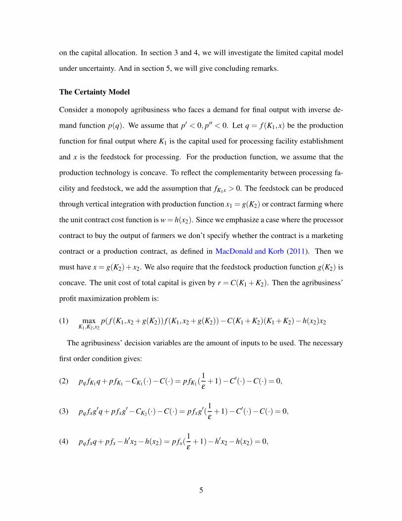
The Certainty Model

Consider a monopoly agribusiness who faces a demand for final output with inverse de-

mand function p(q). We assume that p′ < 0, p′′ < 0. Let q = f (K1,x) be the production

function for final output where K1 is the capital used for processing facility establishment

and x is the feedstock for processing. For the production function, we assume that the

production technology is concave. To reflect the complementarity between processing fa-

cility and feedstock, we add the assumption that fK1x > 0. The feedstock can be produced

through vertical integration with production function x1 = g(K2) or contract farming where

the unit contract cost function is w= h(x2). Since we emphasize a case where the processor

contract to buy the output of farmers we don’t specify whether the contract is a marketing

contract or a production contract, as defined in MacDonald and Korb (2011). Then we

must have x = g(K2)+ x2. We also require that the feedstock production function g(K2) is

concave. The unit cost of total capital is given by r =C(K1 +K2). Then the agribusiness’

profit maximization problem is:

maxK1,K2,x2

p( f (K1,x2 +g(K2)) f (K1,x2 +g(K2))−C(K1+K2)(K1+K2)−h(x2)x2(1)

The agribusiness’ decision variables are the amount of inputs to be used. The necessary

first order condition gives:

pq fK1q+ p fK1

−CK1(·)−C(·) = p fK1

(1

ε+1)−C′(·)−C(·) = 0,(2)

pq fxg′q+ p fxg′−CK2(·)−C(·) = p fxg′(

1

ε+1)−C′(·)−C(·) = 0,(3)

pq fxq+ p fx −h′x2 −h(x2) = p fx(1

ε+1)−h′x2 −h(x2) = 0,(4)

5

where ε denotes the demand elasticity. The first order conditions imply that the

marginal value product of each input must equal to the marginal cost of the input. Here

the marginal value product is calculated by the marginal revenue of final output multiplied

by the marginal product of each input. Notice that monopoly firms will only operate in

elastic portion of demand curve, then we may divide 1+ 1ε

on each side of the equalities.

Therefore, from equation (3) and (4), we should find:

g′ =fK1

fx=

(K1 +K2)C′(·)+C(·)

h′x2 +h(x2).(5)

Notice that the first equality implies that the marginal rate of technical substitution be-

tween capital and feedstock for final output must equal to the marginal product of self-

produced input: MRT S1K,x = MP2

K2. The intuition is quite straightforward: if MRT S1

K,x >

MP2K2

, then the agribusiness could reach the same final output level by allocating one less

unit of capital on producing the input and one more unit of capital on processing the final

product. By doing so, the production plan requires MRT S1K,x less units of total input x

and producing MP2K2

less units of inputs x2. Therefore, the original final output production

amount is still feasible but using less units of total input. Meanwhile, if MRT S1K,x < MP2

K2,

by the same logic, it is efficient to allocate more capital on producing the input. Thus, when

the production plan is optimized, we must have MRT S1K,x = MP2

K2.

The other equality in equation (5): g′ = (K1+K2)C′+C(K1+K2)

h′x2+h(x2)implies that, at optimal point,

the marginal product of K2 equal to the relative marginal cost of capital and of contract

feedstock production. In particular, when marginal cost of capital and contracted feedstock

production are constant, we have the following lemma:

Lemma 1 The capital devoted to self-produced feedstock is fixed and independent of out-

put demand.

Proof See appendix A1 for the proof.

6

The illustration of the analysis is given in figure 2 when the unit cost of capital and

contracted feedstock are constant. In this case, we know that equation (5) becomes g′(K2)=

fK1fx

= rw

. Here the equation g′(K2) =rw

gives a unique solution of K∗

2 . At the same time,

the equality MRTS1K,x = MP2

K2means that, at optimal, the tangent line of the isoquant curve

of final output must also equal to rw

. Notice that, for final output, the condition of marginal

revenue equaling to marginal cost of output determines the optimal final output level. And

this condition specifies a unique isoquant curve that MRT S1K,x should equal to MP2

K2. Then,

all of the decision variables are determined.

The lemma provides a basis for the comparative statics analysis. Especially, we would

like to see how capital allocation changes with respect to higher unit cost of capital. More-

over, we may explore special cases such as when the agribusiness has monopsony power

over contract farming of feedstock production or over capital. The basic conclusions are

given in the following corollary.

Corollary 2 If the agribusiness has monopsony power over contract farming of feedstock

production, then more capital will be allocated to self-production of feedstock. If the

agribusiness has monopsony power over capital, then less capital will be allocated to self-

production of feedstock.

Proof See Appendix A2 for the proof.

The rationale behind the corollary is that when the agribusiness has monopsony power

over contracted feedstock production, he/she may exert the monopsony power by using less

contract farming as the unit cost of contracted feedstock is increasing. Then, in order to

produce the deficit of feedstock, the agribusiness has to use more capital on producing the

input. Similarly, when the agribusiness has monopsony power over capital, less capital will

be used. Consequently, the amount of self-produced feedstock will be reduced and more

feedstock has to be contracted-out.

7

The fundamental comparative statics exercise we are looking for is how would a agribusi-

ness allocate capital when the capital is more expensive. This question is pertinent when

a agribusiness faces credit constraint because when a agribusiness faces tighter credit con-

straint, the shadow cost of capital is larger which is equivalent to higher price of capital. Our

first proposition gives an answer to this question under the scenario of constant marginal

cost of capital and contracted feedstock.

Proposition 3 As capital becomes more expensive, the agribusiness will produce less final

output; less capital will be used on self-produced feedstock and facility building; more

feedstock production will be contracted out.

Proof See appendix A3 for the proof.

The proof of the proposition is illustrated in figure 3. The original optimal point is

K∗

1 ,K∗

2 ,x∗. As r increases, we should have the marginal cost of final output being increased.

As a consequence, marginal revenue equal to marginal cost condition implies that the final

output should be decreased from isoquant Q∗ to isoquant Q∗∗. At the same time, as r

increases, the tangent line to the g(K2) function must become steeper. And the new tangent

line should also be tangent to the new isoquant curve Q∗∗. As shown in the graph, we can

easily see that K∗

1 ,K∗

2 ,x∗ all decrease as r increases. Also notice that the proportion of x1

in x is decreased. Therefore, the contracted portion of feedstock must increase.

The other comparative statics question we want to solve is that how agribusiness’ input

decisions will respond to shifts in output or input market parameter changes. Here, we

look at two specific cases: changes in the demand elasticity of final output and in the

supply elasticity of feedstock from contractees.

Proposition 4 If the demand of the final product is less elastic, then less final product will

be produced and the share of the in-house production is larger. If the supply of input from

contractees is less elastic, then less final output will be produced and the share of in-house

production is larger.

8

Proof See appendix A4 for the proof.

The intuition behind Proposition 4 is that, when demand of the final product is less elastic,

the marginal revenue curve becomes steeper, which makes it intersect the marginal cost

curve at a lower production level. And the reduction in output production is achieved by

reducing both input uses. But, we know that capital usage on feedstock does not change

as demand side variables change, therefore, we must have increased share of in-house

feedstock production. When the supply of input from contractees is less elastic, marginal

cost curve is steeper. And the other arguments follow the similarly.

Production Uncertainty

Now, we consider the case of uncertainty in final output production. The underlying mo-

tivation is that a agribusiness may develop new technology in processing, and the uncer-

tainty in the new technology makes the quantity of final output production uncertain. For

instance, a biofuel refinery may consider using second generation feedstock to produce

biofuel, but the processing technology, conversion rate in this case, is not mature. Let

q = θ f (K1,x) denote the final output, where θ is a random variable with mean θ̂ and vari-

ance σ2. One possible interpretation of θ is the processing technology improvement. Let

π = p · θ f (K1,x2 + g(K2)− r(K1 +K2)−wx2 denote the agribusiness’ profit. And, using

the framework by Sandmo (1971), the firm’s problem is to maximize the utility from profit.

i.e.,

maxK1,K2,x2

EU [p ·θ f (K1,x2 +g(K2)− r(K1+K2)−wx2]

where we assume that U ′(π) > 0,U ′′(π) < 0. We are most interested in how such uncer-

tainty may cause different allocation of resources than the deterministic case. And we have

the following proposition:

9

Proposition 5 Under production uncertainties, expected final output production is less

than certainty case; both capital used on processing and contracted feedstock level are

less than certainty amount; the capital on feedstock production remains the same.

Proof See appendix A5 for the proof.

Uncertainty in Contract Farming

As Acemoglu, Johnson, and Mitton (2009) introduced in their model, there is also uncer-

tainty in contract farming: contractees may default the contract. Consider the case that

agribusiness is uncertain about the level of feedstock can be received from farmers. Let

θ be the proportion of x2 that is finally received. The processor can expect to receive a

proportion of θ̂ . Let π = p · f (K1,x2 +g(K2)− r(K1 +K2)−wθx2 and again, we assume

that the agribusiness is maximizing the expected utility of profit.

maxK1,K2,x2

EU [p · f (K1,x2 +g(K2)− r(K1 +K2)−wθx2],(6)

where we again assume that U ′(π)> 0,U ′′(π)< 0.

Proposition 6 With uncertainty in contracted feedstock, expected final output production

is less than certainty case; both capital used on processing and contracted feedstock level

are less than certainty amount; the capital on feedstock production is more than certainty

amount.

Proof See appendix A6 for the proof.

The result of this proposition reflects the essence of the Sandmo model: uncertainty

will lead to reduction in output production. In this particular case, the decrease in output

production comes from the reduction in both of the input levels. Decrease in K1 means

that the agribusiness would build smaller processing facility, which in turn requires less

total feedstock. However, the magnitude in the reduction of contracted feedstock is greater

than the reduction of total feedstock being required. Consequently, the agribusiness has

10

to use more capital on feedstock production to meet the deficit. One way to look at this

proposition is that when a processor agribusiness has better information about contracted

farmers, more output will be produced and more contract farming will be carried out. This

result may be another possible way to explain the growth of contract farming over time: as

the processors know more about the contractees, contract farming is more likely to happen.

To see the interaction between credit constraint and uncertainty, we would like to see the

comparative statics of the input levels with respect to cost of capital under contract uncer-

tainties. When the utility function of the agribusiness is decreasing absolute risk aversion,

it is easy to see that higher cost of capital will have a direct effect and an indirect effect:

the direct effect is that higher cost of capital will lower final output production and self-

produced feedstock and increase contracted feedstock, as demonstrated in proposition 3;

however, higher cost of capital also indirectly affect the capital allocation in that it de-

crease the wealth of the agribusiness and consequently makes the agribusiness to be less

able to bear risks. As Sandmo (1971) suggests, the indirect effect will further lower the

contracted feedstock production and makes the total effect on self-production of feedstock

ambiguous.

Concluding Remarks

In this article, we investigate an agribusiness’ decision, in both certainty and uncertainty

cases, on capital allocation when it has the option of acquiring the feedstock through con-

tracts and self-production. Our analytical model first establishes the fact that, in the cer-

tainty case, a monopoly’s capital allocated on input production is independent of final out-

put demand. And, at optimal, the marginal rate of technical substitution between input and

capital used on output production must equal to the marginal product of capital on input

production. Furthermore, our results show that when agribusiness have monopsony power

over capital or contractees’ supply of input is elastic, there will be more contract farming.

When there is uncertainty in output production, expected final output will be less than cer-

11

tainty case and less capital will be allocated to self-production of the input. When there is

uncertainty in contracted feedstock, expected final output will be less than certainty case

and more capital will be allocated to self-production of the input.

The key proposition of the model is that contract farming is especially plausible when a

agribusiness faces higher cost of capital or credit constraint. Our results can be empirically

tested by and applied to many real world applications. For instance, our model could partly

answer why Tyson Foods would use contracts to raise chickens– the core competence of

Tyson Foods is in processing and marketing its final product and the feedstock requires

huge amount of capital. Thus, it will allocate more capital on building processing facility

and less on raising the chickens. Similarly, McDonald’s may find it more profitable to

franchise out its chain stores rather than run a store itself as developing another chain store

is costly. Our model could also provide guidance for new industries. For example, a biofuel

refinery in Brazil may face the capital allocation problem on refining facility and growing

the sugarcane. Our model suggests that the refinery should use contract farming as a tool to

deal with its credit constraint and, use more contract farming as the productivity of farmers

becomes more certain.

It should be noted that the model may behave differently if we consider the dynamics

version of the model, especially when the agribusiness enjoys a learning-by-doing effect

when it develops the feedstock. In that case, the value of self-production of the feedstock

may grow over time, then there may exist an optimal time to switch from self-production

to contract farming, and we leave this as a direction for future research.

12

References

Acemoglu, D., S. Johnson, and T. Mitton. 2009. “Determinants of Vertical Integration:

Financial Development and Contracting Costs.” Journal of Finance 64:1251–1290.

Alexander, C., R. Goodhue, G. Rausser, et al. 2000. “Do quality incentives matter?” Work-

ing Paper-Department of Agricultural and Resource Economics, University of Califor-

nia, Davis, pp. .

Bierlen, R., L.D. Parsch, and B.L. Dixon. 1999. “How cropland contract type and term

decisions are made: evidence from an Arkansas tenant survey.” The International Food

and Agribusiness Management Review 2:103–121.

Boehlje, M., L.F. Schrader, J. Royer, R. Rogers, et al. 1998. “The industrialization of agri-

culture: questions of coordination.” The industrialization of agriculture: vertical coor-

dination in the US food system., pp. 3–26.

Cheung, S. 1969. The theory of share tenancy.. Chicago/London: Univ. Chicago Press.

Du, X., L. Lu, and D. Zilberman. 2013. “Contracting Farming in Biofuel Sector: A Sur-

vey.” Working Paper, Department of Agricultural and Resource Economics, University

of California, Berkeley.

Feder, G. 1977. “The impact of uncertainty in a class of objective functions.” Journal of

Economic Theory 16:504–512.

Franken, J.R., J.M. Pennings, and P. Garcia. 2009. “Do Transaction Costs and Risk Pref-

erences Influence Marketing Arrangements in the Illinois Hog Industry?” Journal of

Agricultural and Resource Economics 34:297–315.

Glover, D., J.v. Braun, E. Kennedy, et al. 1994. “Contract farming and commercializa-

tion of agriculture in developing countries.” Agricultural commercialization, economic

development, and nutrition., pp. 166–175.

Goodhue, R.E. 2000. “Broiler Production Contracts as a Multi-Agent Problem: Common

Risk, Incentives and Heterogeneity.” American Journal of Agricultural Economics 82:pp.

13

606–622.

Hueth, B., and E. Ligon. 2002. “Estimation of an efficient tomato contract.” European

Review of Agricultural Economics 29:237–253.

Jaynes, G.D. 1982. Economic Theory and Land Tenure, in H. Binswanger, and M. Rosen-

zweig, eds., Rural Labor Markets in Asia: Contractual Arrangements, Employment and

Wages, New Haven: Yale University Press.

Katchova, A.L., and M.J. Miranda. 2004. “Two-step econometric estimation of farm char-

acteristics affecting marketing contract decisions.” American Journal of Agricultural

Economics 86:88–102.

Knoeber, C., and W. Thurman. 1995. ““Don’t Count Your Chickens...”: Risk and Risk

Shifting in the Broiler Industry.” American Journal of Agricultural Economics 77:486–

496.

MacDonald, J.M., and P. Korb. 2011. “Agricultural Contracting Update: Contracts in

2008.” Working paper, EIB-72. U.S. Dept. of Agriculture, Econ. Res. Serv.

Pennings, J.M., and B. Wansink. 2004. “Channel contract behavior: The role of risk atti-

tudes, risk perceptions, and channel members’ market structures.” The journal of busi-

ness 77:697–724.

Rubin, P. 1978. “Theory of the Firm and the Structure of the Franchise Contract, The.” JL

& Econ. 21:223.

Ruf, F. 2009. “Developing Smallholder Rubber Production.” Ex Post. Agence Française de

Développement, pp. .

Sandmo, A. 1971. “On the theory of the competitive firm under price uncertainty.” The

American Economic Review 61:65–73.

14

Figures

2001-2002

2008

0

20

40

60

80

100

Corn Sugar

Beets

Cotton Fruit Vegetables Cattle Hogs Poultry

and

eggs

Figure 1. Share of commodity production under contract in 2001 and 2008

Source: MacDonald and Korb (2011)

15

x

K1K2 K∗

1K∗

2

x∗1

x∗

MRT S1K,x

MP2x2

Production Function of Self-produced Input x1

Isoquant for Final Output Production Function

Figure 2. Illustration of capital allocation

16

x

K1K2 K∗∗

1 K∗

1K∗∗

2K∗

2

x∗∗1

x∗1

x∗∗

x∗

Q∗∗

Q∗

Production Function of Self-produced Input x1

Isoquant for Final Output Production Function

Figure 3. Illustration of capital allocation when capital is more expensive

17

AJAE Appendix for The Economics of Contract Farming:

A Credit and Investment Perspective

A1. Proof for Lemma 1

Proof We have established earlier that

g′ =(K1 +K2)C

′(·)+C(·)

h′(x2)x2 +h(x2).(7)

Thus, when marginal cost of capital and contracted feedstock production are constant,

we have C′ = h′ = 0. And we have g′ = rw

. Therefore, the optimal K2 is given by:

K∗

2 = (g′)−1(r

w).(8)

Clearly, demand side variables are not involved in optimal K2.

A2. Proof for Corollary 2

Proof Suppose the agribusiness has monopsony power over contract farming of feedstock

production, then equation (5) implies: g′(K2) =r

w+h′x2. Let K∗∗

2 be the optimal capital

under this scenario. And we have:

g′(K∗∗

2 ) =r

h′x2 +w<

r

w= g′(K∗

2 ).(9)

The inequality holds because h′(x2)> 0. Notice that g′′ < 0 and g′(K∗∗

2 )< g′(K∗

2 ), we must

have K∗∗

2 > K∗

2 . The second statement follows from the same proof.

A3. Proof for Proposition 3

Proof We first derive the Hessian for the problem. Let a = p′q+ p and b = a′ = p′′q+2p′.

Since a = p(1+ 1ε), we must have a > 0. Also notice that b < 0 by the assumption of

1

p′′ < 0. Then the Hessian for the problem can be written as:

HHH =

a fK1K1+b f 2

K1a fK1xg′+b fK1

fxg′ a fK1x +b fK1fx

a fK1xg′+b fK1fxg′ a fxx(g

′)2 +b f 2x (g

′)2 +a fxg′′ a fxxg′+b f 2x g′

a fK1x +b fK1fx a fxxg′+b f 2

x g′ a fxx +b f 2x

.(10)

Since we have a profit maximization problem, the second order condition requires that HHH

is negative definite. Therefore, we have |HHH|< 0. By total differentiation, we can see that:

HHH

dK∗

1dr

dK∗

2dr

dx∗2dr

=

1

1

0

.(11)

We use HHH i j to denote the submatrix of HHH that eliminates the ith row and jth column of HHH.

By Cramer’s rule, we find that:

dK∗

1

dr=

|HHH11|− |HHH21|

|HHH|.(12)

Since HHH11 is a principal minor of HHH, and HHH is a negative definite matrix, we must have

|HHH11|> 0. Moreover, it can be easily verified that |HHH21|= 0 (the second column of HHH21 is

the first column multiplying g′). Therefore, we have:

dK∗

1

dr=

|HHH11|− |HHH21|

|HHH|< 0.(13)

Again, by Cramer’s rule, we get:

dK∗

2

dr=

−|HHH12|+ |HHH22|

|HHH|< 0,(14)

which comes from the fact that |HHH22| > 0 as HHH22 is another principal minor of HHH, and the

fact that |HHH12|= 0 (the first row of HHH12 is the second row multiplying g′).

To determine the sign ofdx∗2dr

, first notice thatdx∗2dr

=|HHH13|−|HHH23|

|HHH|. Use the fact that |HHH22|=

|HHH23|g′, and |HHH22| > 0, we have |HHH23| > 0. In order to determine the sign of |HHH13|, we

2

explicitly write down the expression of |HHH13|:

|HHH13|=−a fxg′′(a fK1x +b fK1fx).(15)

Once we can show that a fK1x + b fK1fx < 0, then it follows immediately that

dx∗2dr

> 0. To

show that a fK1x + b fK1fx < 0, we first notice that |HHH11| > 0 as it is a principal minor of

matrix |HHH| > 0. Here |HHH11| = a fxg′′(a fxx +b f 2x ). Then, in order for |HHH11| to be positive,

we must have:

a fxx +b f 2x < 0.(16)

Meanwhile, from |HHH22| > 0, we must have (a fxx +b f 2x )(a fK1K1

+b f 2K1) > 0, and thus we

have:

a fK1K1+b f 2

K1< 0.(17)

Using equations (16) and (17), we get: fx >

√

−a fxx

b, fK1

>

√

−a fK1K1

b. Now, we get:

(18) a fK1x +b fK1fx < a fK1x +b

√

a2 fK1K1fxx

b2

< a fK1x −

√

a2 fxx fK1K1<

√

a2 fxx fK1K1−

√

a2 fxx fK1K1= 0

Therefore, as explained earlier, we must havedx∗2dr

> 0. To do the comparative statics for

dq∗

dr, we first note that

dq∗

dr= fK1

dK∗

1

dr+ fxg′

dK∗

2

dr+ fx

dx∗2dr

,(19)

which can be written as:

dq∗

dr=

fK1|HHH11|+ fxg′|HHH22|+ fx(|HHH13|− |HHH23|)

|HHH|.(20)

It can be verified that |HHH22| = |HHH23|g′, |HHH11| = a fxg′′(a fxx + b f 2

x ), and |HHH13| =

−a fxg′′(a fK1x +b fK1fx). Then, we have:

dq∗

dr=

a2 fxg′′( fxx fK1− fK1x fx)

|HHH|< 0,(21)

3

as fxx < 0, fK1x > 0, g′′ < 0 and |HHH|< 0.

A4. Proof for Proposition 4

Proof In this case, total differentiation with respect to K1,K2,x2,ε , we get the following

matrix form equality:

HHH

dK∗

1dε

dK∗

2

dε

dx∗2dε

= ε−2

p fK1

p fxg′

p fx

,(22)

where HHH is the Hessian of the maximization problem as defined in (10). And we use HHH i

to denote the matrix that replaces the ith column of HHH by ε−2 [p fK1

p fxg′ p fx]T

. Using

Cramer’s rule, we have:

dK∗

1

dε=

|HHH1|

|HHH|,(23)

where |HHH1| = ε−2

∣

∣

∣

∣

∣

∣

∣

∣

∣

∣

p fK1a fK1xg′+b fK1

fxg′ a fK1x +b fK1fx

p fxg′ a fxx(g′)2 +b f 2

x (g′)2 +a fxg′′ a fxxg′+b f 2

x g′

p fx a fxxg′+b f 2x g′ a fxx +b f 2

x

∣

∣

∣

∣

∣

∣

∣

∣

∣

∣

. Notice

that |HHH1| = ε−2

∣

∣

∣

∣

∣

∣

∣

∣

∣

∣

p fK1a fK1xg′+b fK1

fxg′ a fK1x +b fK1fx

0 a fxg′′ 0

p fx a fxxg′+b f 2x g′ a fxx +b f 2

x

∣

∣

∣

∣

∣

∣

∣

∣

∣

∣

= a2p fxg′′ε−2( fK1fxx −

fx fK1x)> 0, we havedK∗

1dε

=|HHH1|

|HHH|< 0.

Since K∗

2 is not affected by demand side variables, we havedK∗

2dε

= 0. We can verify this

by checking |HHH2|= 0 (this is true because the second row of |HHH2| is a multiple of the third

row.

Again, Using Cramer’s rule, we have:

dx∗2dε

=|HHH3|

|HHH|,(24)

4

where |HHH3| = ε−2

∣

∣

∣

∣

∣

∣

∣

∣

∣

∣

a fK1K1+b f 2

K1a fK1xg′+b fK1

fxg′ p fK1

a fK1xg′+b fK1fxg′ a fxx(g

′)2 +b f 2x (g

′)2 +a fxg′′ p fxg′

a fK1x +b fK1fx a fxxg′+b f 2

x g′ p fx

∣

∣

∣

∣

∣

∣

∣

∣

∣

∣

=

ε−2

∣

∣

∣

∣

∣

∣

∣

∣

∣

∣

a fK1K1+b f 2

K1a fK1xg′+b fK1

fxg′ p fK1

0 a fxg′′ 0

a fK1x +b fK1fx a fxxg′+b f 2

x g′ p fx

∣

∣

∣

∣

∣

∣

∣

∣

∣

∣

. Then we can see that

|HHH3|= a2p fxg′′ε−2( fx fK1K1− fK1

fK1x)> 0.(25)

Therefore, we havedx∗2dε

=|HHH3|

|HHH|< 0. Since K∗

2 does not change, we know in-house feedstock

production does not change. But x∗2 have decreased, we know that the share of in-house

feedstock production is larger.

Since

dq∗

dε= fK1

dK∗

1

dε+ fxg′

dK∗

2

dε+ fx

dx∗2dε

,(26)

anddK∗

1dε

< 0,dK∗

2dε

= 0,dx∗2dε

< 0, we must have

dq∗

dε< 0.(27)

When supply of input from contractees is less elastic, we write the equation (4) in the form

of: p fx(1+1ε) = w(1+ 1

η). And we rewrite equation (5) as g′ = r

w(1+ 1η). As η decreases,

we should observe that g′ also decreases and K∗

2 increases. Other comparative static results

follow from the same procedure.

A5. Proof for Proposition 5

Proof The first order condition w.r.t K1 is:

E{u′(π)[pθ fK1− r]}= 0

5

Then

E{u′(π)[pθ fK1− pθ̂ fK1

]}= E{u′(π)[pθ̂ fK1− r]}

Notice that

π = Eπ +(θ − θ̂ )p f (·)

Thus, for all θ > θ̂ , we must have u′(π)< u′(Eπ). And consequently,

u′(π)(θ − θ̂ )> u′(Eπ)(θ − θ̂),∀θ

Therefore,

E{u′(π)[pθ fK1− pθ̂ fK1

]}= p fK1E{u′(π)(θ − θ̂)}> p fK1

E{u′(Eπ)(θ − θ̂)}= 0

But, this implies

pθ̂ fK1> r.

Similarly, we can also show that

pθ̂ fx > w.

These two equations imply that, under uncertainty, both fK1and fx are higher than the

certainty case.

Using the lemmas in Feder (1977), we have the following equality:

fK1

fx= g′(K2) =

r

w

Therefore, the capital used on feedstock production is the same as in certainty case. Now,

take total derivative for fK1and fx, and realizing that K2 doesn’t change, we get:

d fK1= fK1K1

dK1 + fK1xdx2

d fx = fxK1dK1 + fxxdx2

6

It can be easily verified that in order for fK1and fx to be both increasing, the only possibility

is dK1,dx2 < 0, which means both capital used on processing and contracted feedstock level

are less than certainty amount. Also notice that:

dq = fK1dK1 + fxdx2 < 0

which means the final output level is less than certainty case as well.

A6. Proof for Proposition 6

Proof The first order condition yields:

p fK1= p fxg′ = r

Meanwhile,

E{u′(π)[p fx −wθ ]}= 0

Then we get:

E{u′(π)[p fx −wθ̂ ]}= E{u′(π)w(θ − θ̂)}

Since

π = Eπ −w(θ − θ̂)x2

We have, for all θ > θ̂ , u′(π)> u′(Eπ). Thus,

u′(π)(θ − θ̂ )> u′(Eπ)(θ − θ̂)

. And consequently, p fx > wθ̂ . In summary, comparing to certainty case, we have larger

fx and fK1remains unchanged. Therefore, from

fK1fx

= g′(K2), we know that g′(K2) must

have been decreased, which means K2 is larger than the certainty case. Now, we take total

derivative for fx, fK1:

d fK1= fK1K1

dK1 + fK1xdx = 0

7

And

d fx = fxK1dK1 + fxxdx

From the first equation, we get:

dK1

dx=−

fK1x

fK1K1

Thus,

d fx

dx=

fxx fK1K1− f 2

K1x

fK1K1

< 0

. Then, in order for fx to be increasing, the total feedstock amount must have been de-

creased. Also notice that in order for d fK1= fK1K1

dK1 + fK1xdx = 0 to hold, we cannot

have dK1 > 0. Then, K1 must have been decreased. Since the total feedstock level and K1

are both decreasing, from the equation:

dq = fK1dK1 + fxdx

we know that dq < 0, which means the total output is less than the certainty case.

8