The Economics of the Mandatory Renewable Energy Target

(MRET)

Israel del Mundo and Ian Wills Department of Economics

Monash University Clayton 3800

iddel1@student.monash.edu.au ian.wills@buseco.monash.edu.au

ABSTRACT

In response to increasing awareness of climate change, the Howard government implemented the Mandatory Renewable Energy Target (MRET) in 2001. It requires electricity wholesalers to source an additional 9500 GWh of electricity from renewable sources by 2010. Electricity wholesalers are required to subsidise renewable energy generators by purchasing Renewable Energy Certificates (RECs) equivalent to the target; failure to do so incurs a penalty of $40 per megawatt. Economic analysis is used to investigate the design and likely operation and limitations of the MRET. Key words: energy policy, climate change, renewable energy, Mandatory Renewable Energy Target

2

GLOSSARY BAA – Backing Australia’s Ability FF – Fossil fuels GHG – greenhouse gases GP – Green Power GWh – gigawatt hours (1GWh = 1000MWh) MRET – Mandatory Renewable Energy Target MWh – megawatt hours NEM – National Electricity Market New RE – Renewable Energy over and above ‘current’ (1997) levels ORER – Office of the Renewable Energy Regulator RE – Renewable Energy REC – Renewable Energy Certificates RPP – Renewable Power Percentage Note: the terms “wholesaler” and “liable parties” will be used interchangeably in the text.

3

INTRODUCTION The literature dealing with climate change has focused on abating Greenhouse Gas

(GHG) emissions while keeping fossil fuels as the primary energy source. This glosses over Renewable Energy (RE), which is the better long-term proposition (see “Advantages and Disadvantages of RE” section).

More research on the economics of renewable energy is needed. This is not to say that we should abandon CO2 abatement. Because of lower costs, Fossil Fuels are likely to play a big part in Australian and global energy use in the foreseeable future. RE’s current technological state and the intermittent nature of its supply means that a reliable and cheap energy source like coal will be needed for some time to maintain living standards. Abatement technology should, therefore, be developed concurrently with RE technology. Australia’s primary vehicle for promoting RE is the Mandatory Renewable Energy Target (MRET), which obligates electricity wholesalers to buy a specified proportion of RE1. It aims to source an additional 9500 GWh of electricity from RE generators by 2010.

Section I of the paper looks at the justification for an RE target, and investigates the implications on the National Electricity Market (NEM) of imposing an RE policy. Section II then attempts to explain the basic economics behind the MRET. This section focuses on the workings of Renewable Energy Certificates (RECs) markets and some of the issues in its operation. A brief evaluation of the measure’s potential to promote Renewable Energy in Australia is then provided.

SECTION I THE MRET IN BRIEF In 1997, the Howard government launched several initiatives to combat climate change. One initiative gave rise to the MRET. It aims to source an additional 9,500 GWh per year from RE by 2010, and operates until 2020.

Australia sourced 9.9% of electricity from RE in 1997, mostly from hydroelectricity in Tasmania. The other states made much less use of RE (see Appendix 1).

With certain exceptions, electricity wholesalers on grids of over 100MW installed capacity are required to contribute towards the additional 9500 GWh in proportion to their market share2 (known as their Renewable Power Percentage – RPP). For example, if a wholesaler has a 10% market share in 2004, they must contribute 10% of the target for 2005. Because of the NEM’s growth, wholesalers usually purchase electricity from a ‘pool’, not directly from the generator. Liable parties must therefore ‘prove’ their contribution towards the scheme by purchasing an amount of RECs equivalent to their RPP, where 1 REC represents 1 MWh of new RE generated.

To prevent last-minute investment in RE, interim targets have been set (see Table 1). Failure to comply incurs a $40/MWh shortfall charge.

Table 13 – Interim Targets for MRET

YEAR Required additional GWh 2001 300 2002 1100 2003 1800

1 Other significant GHG emitters, particularly the transport sector and manufacturing, are not included in the measure. However, the electricity industry accounts for nearly 50% of Australia’s energy-related emissions (www.abs.gov.au [1]), so it is a good place to begin an RE initiative. 2 “Overview of the Mandatory Renewable Energy Target” – www.orer.gov.au/overview.html 3 Ibid

4

2004 2600 2005 3400 2006 4500 2007 5600 2008 6800 2009 8100 2010-2020 9500 THE CASE TO REDUCE HYDROCARBON ENERGY USE: CLIMATE CHANGE

It is common knowledge that the burning of fossil fuels emits GHGs, contributing to global warming. (see Appendix 2 for a simple explanation of global warming)

GHGs persist for long periods, and accumulate in the atmosphere, but climate change is not immediately observable. This negative externality involves a lag, whose magnitude is uncertain. Global warming is thus an inter-temporal problem because today’s energy consumption adversely affects future generations. With over a century of emissions behind us, and rising energy demand ahead of us4, GHG emission reduction is becoming an urgent topic.

The Intergovernmental Panel on Climate Change (IPCC) forecasts world temperatures to increase by 1.4-5.80C above 1990 levels by 2100. Such a rise is expected to significantly alter the global ecology. Global rainfall pattens will be affected, summer continental drying will lead to increased risk of droughts, and there will be an “increase in tropical cyclone mean and peak precipitation intensities”5. Businesses are already bracing themselves for the disruptions ahead: IAG, Australia’s largest insurer, recently announced its intentions to reinsure a large portion of its policies in north-eastern Australia because of the region’s exposure to global warming-induced threats6.

Besides the inter-temporal externality of climate change, hydrocarbons produce “current” externalities in the form of smog. Smog has adverse effects on health, creating economic costs. GHG emissions and smog are expected to soar as the world’s developing nations rapidly industrialise and increase energy demand (e.g. China and India). ADVANTAGES and DISADVANTAGES OF RE

RE has the potential to supply energy demands without the adverse ecological effects because it emits very little or no GHGs. Furthermore, increasing the use of RE allows greater self-sufficiency in energy supply. Because “inputs” (wind, sun, etc.) are home-grown, the economy is less exposed to price fluctuations in imported energy inputs. This stabilises prices in general and reduces uncertainty in the economy as a whole. Furthermore, these inputs are free, at least partially offsetting the high upfront capital costs of RE in the long run.

There is also great potential to develop an export market for RE technology. According to government sources, Australia is a leader in photovoltaics, as well as wind, biomass, and wave technologies7. The introduction of the MRET has seen exports rise from around $140 million in 2000/01 to over $250 million in 2003/048. More export growth is expected in the future, particularly exports to South-East Asia.

4 By 2014-15, total energy production in Australia is projected to increase by 55% over 1997-98 levels, with electricity generation a major contributor. (www.abs.gov.au [2]) 5 Cline, W.R., “Meeting the Challenge of Global Warming”, Copenhagen Consensus Challenge Paper, 2004 – p.2 6 Gottliebsen, R., “Insurers raise the eco-alarm”, The Weekend Australian, September 4-5, 2004 – p.36 7 Securing Australia’s Energy Future, Commonwealth of Australia, 2004 – p.33 8 Renewable Opportunites: A Review of the Renewable Energy (Electricity) Act 2000, September 2003, Australian Greenhouse Office – p.23

5

Of course, the intermittent nature of key RE sources like wind and solar is a big disadvantage, which is why hydrocarbon sources will dominate for the foreseeable future.

Moreover, RE may not all be free of negative externalities. Wind generators are noisy, and perhaps unsightly. Hydro generators can affect the aquatic environment, and must share the resource with other users9. Advances in technologies and sound planning of projects may be able to deal with many of these issues.

WHY FREE MARKETS WILL FAIL TO PROMOTE RE If left to market forces, the amount of new renewable energy generation will not rise by as much as the MRET in the short to medium term simply because RE is not yet cost-competitive with conventional energy (see Table 2). Table 210

Technology Average Production Cost ($/MWh) Coal pf-fired 24-36 Gas combined cycle 30-40 Co-firing biomass 34-52 Bagasse (existing plant) 35-55 Bagasse (new) 44-65 Small scale hydro 24-70 Landfill gas 34-71 Solar hot water 44-70 Biomass 34-81 Agricultural biogas 44-81 Municipal waste 44-96 Wind grid connected 74-105 Solar thermal 150-220 Solar PV 440-750

With no government intervention, resource substitution would occur. As fossil fuels are depleted over time, their prices would increase until there is finally incentive to develop and adopt RE technologies in earnest. However, coal reserves are estimated to last for 224 years under current production patterns11, so resource substitution is unlikely to spur significant RE development this century. A well-known problem with markets is that they ignore externalities. As previously mentioned, fossil fuel-related externalities are felt by future generations. Much of the debate about abating CO2 concerns the costs incurred by today’s generations, whereas future generations benefit12. This partly explains the lack of incentive to abate today. THE OPTIMUM RE GENERATION We thus find scope for government intervention in the RE sector; but the question of how remains. In this section, we look at how externalities from FF may be represented, and

9 Key Issues in Developing Renewables, International Energy Agency, 1997 – p.33 10 Young, BC, & Allardice, DJ, The Implementation of the 2% Mandatory Renewable Energy Target in Australia, A study commissioned by New Energy and Industrial Technology Development Organisation (NEDO), March 2001 – p.25 11 World Energy Outlook 1998 Edition, International Energy Agency – p.138 12 The size of externalities with an inter-temporal dimension depends on the time horizon (the further the time horizon, the greater are the externalities and associated costs), and the size of discount rates.

6

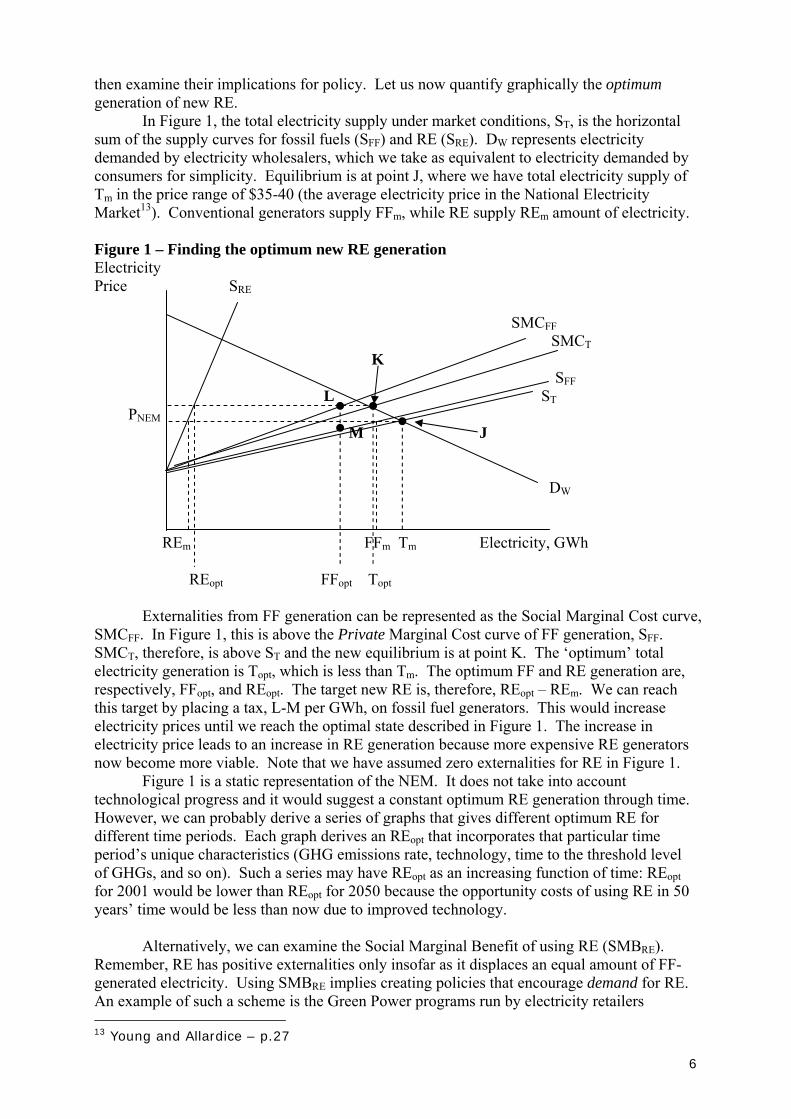
then examine their implications for policy. Let us now quantify graphically the optimum generation of new RE.

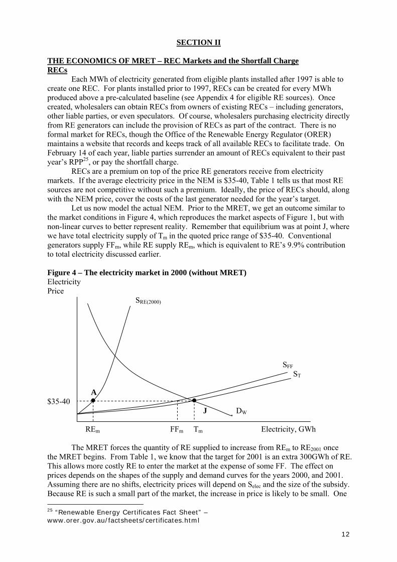
In Figure 1, the total electricity supply under market conditions, ST, is the horizontal sum of the supply curves for fossil fuels (SFF) and RE (SRE). DW represents electricity demanded by electricity wholesalers, which we take as equivalent to electricity demanded by consumers for simplicity. Equilibrium is at point J, where we have total electricity supply of Tm in the price range of $35-40 (the average electricity price in the National Electricity Market13). Conventional generators supply FFm, while RE supply REm amount of electricity. Figure 1 – Finding the optimum new RE generation Electricity Price SRE SMCFF SMCT K SFF L ST PNEM M J DW REm FFm Tm Electricity, GWh REopt FFopt Topt

Externalities from FF generation can be represented as the Social Marginal Cost curve,

SMCFF. In Figure 1, this is above the Private Marginal Cost curve of FF generation, SFF. SMCT, therefore, is above ST and the new equilibrium is at point K. The ‘optimum’ total electricity generation is Topt, which is less than Tm. The optimum FF and RE generation are, respectively, FFopt, and REopt. The target new RE is, therefore, REopt – REm. We can reach this target by placing a tax, L-M per GWh, on fossil fuel generators. This would increase electricity prices until we reach the optimal state described in Figure 1. The increase in electricity price leads to an increase in RE generation because more expensive RE generators now become more viable. Note that we have assumed zero externalities for RE in Figure 1.

Figure 1 is a static representation of the NEM. It does not take into account technological progress and it would suggest a constant optimum RE generation through time. However, we can probably derive a series of graphs that gives different optimum RE for different time periods. Each graph derives an REopt that incorporates that particular time period’s unique characteristics (GHG emissions rate, technology, time to the threshold level of GHGs, and so on). Such a series may have REopt as an increasing function of time: REopt for 2001 would be lower than REopt for 2050 because the opportunity costs of using RE in 50 years’ time would be less than now due to improved technology.

Alternatively, we can examine the Social Marginal Benefit of using RE (SMBRE).

Remember, RE has positive externalities only insofar as it displaces an equal amount of FF-generated electricity. Using SMBRE implies creating policies that encourage demand for RE. An example of such a scheme is the Green Power programs run by electricity retailers 13 Young and Allardice – p.27

7

Australia-wide, in which consumers pay a premium to source a portion of their electricity from RE. However, since the program still has a tiny subscription rate, it is unlikely, by itself, to significantly promote RE. For this reason, we will focus on schemes promoting RE in the NEM, which are likely to have a greater impact (see Appendix 3 for a treatment of schemes that promote consumer demand for RE). ACHIEVING THE OPTIMUM GENERATION

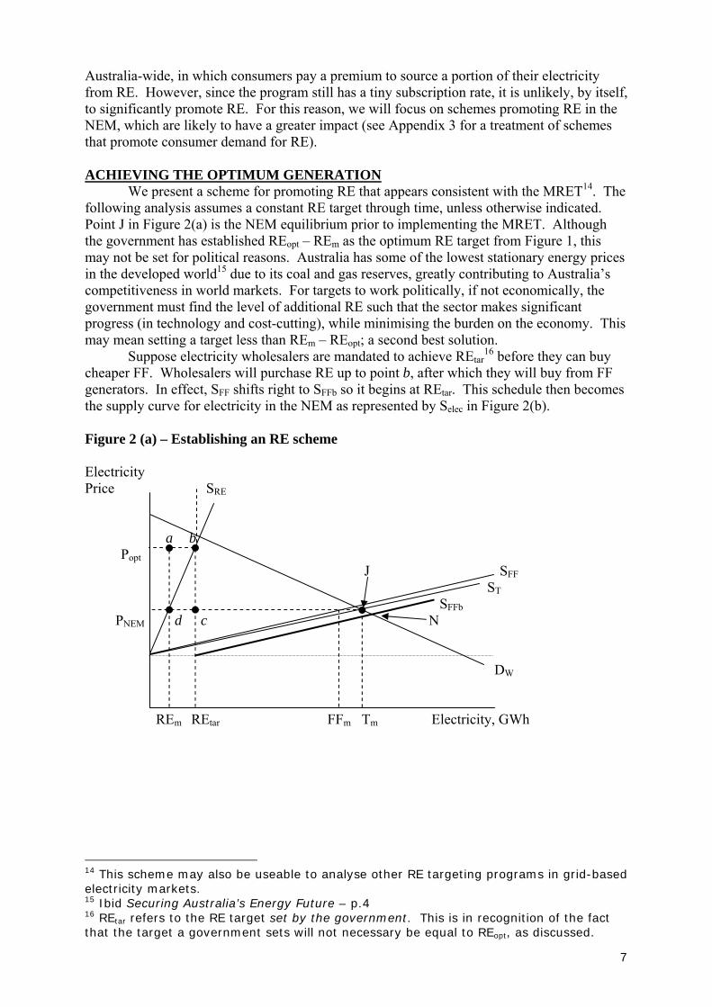
We present a scheme for promoting RE that appears consistent with the MRET14. The following analysis assumes a constant RE target through time, unless otherwise indicated. Point J in Figure 2(a) is the NEM equilibrium prior to implementing the MRET. Although the government has established REopt – REm as the optimum RE target from Figure 1, this may not be set for political reasons. Australia has some of the lowest stationary energy prices in the developed world15 due to its coal and gas reserves, greatly contributing to Australia’s competitiveness in world markets. For targets to work politically, if not economically, the government must find the level of additional RE such that the sector makes significant progress (in technology and cost-cutting), while minimising the burden on the economy. This may mean setting a target less than REm – REopt; a second best solution.

Suppose electricity wholesalers are mandated to achieve REtar16 before they can buy

cheaper FF. Wholesalers will purchase RE up to point b, after which they will buy from FF generators. In effect, SFF shifts right to SFFb so it begins at REtar. This schedule then becomes the supply curve for electricity in the NEM as represented by Selec in Figure 2(b). Figure 2 (a) – Establishing an RE scheme Electricity Price SRE a b Popt J SFF ST SFFb PNEM d c N DW REm REtar FFm Tm Electricity, GWh

14 This scheme may also be useable to analyse other RE targeting programs in grid-based electricity markets. 15 Ibid Securing Australia’s Energy Future – p.4 16 REtar refers to the RE target set by the government. This is in recognition of the fact that the target a government sets will not necessary be equal to REopt, as discussed.

8

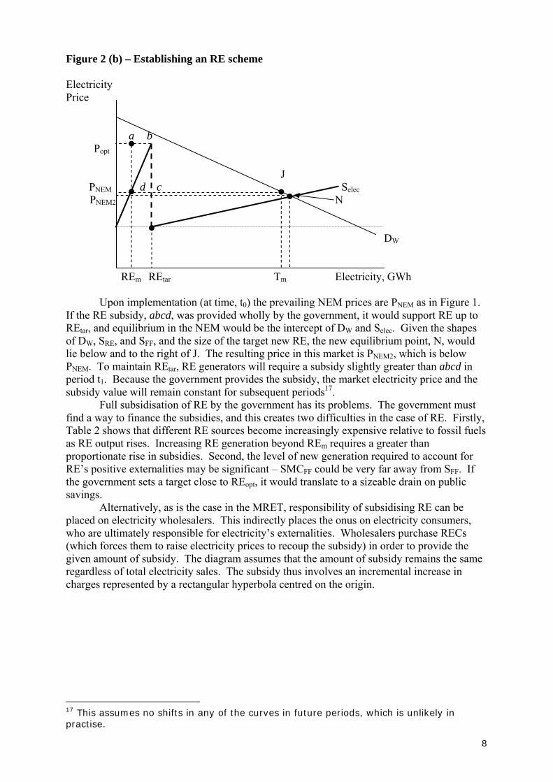
Figure 2 (b) – Establishing an RE scheme Electricity Price a b Popt J PNEM d c Selec PNEM2 N DW REm REtar Tm Electricity, GWh Upon implementation (at time, t0) the prevailing NEM prices are PNEM as in Figure 1. If the RE subsidy, abcd, was provided wholly by the government, it would support RE up to REtar, and equilibrium in the NEM would be the intercept of DW and Selec. Given the shapes of DW, SRE, and SFF, and the size of the target new RE, the new equilibrium point, N, would lie below and to the right of J. The resulting price in this market is PNEM2, which is below PNEM. To maintain REtar, RE generators will require a subsidy slightly greater than abcd in period t1. Because the government provides the subsidy, the market electricity price and the subsidy value will remain constant for subsequent periods17. Full subsidisation of RE by the government has its problems. The government must find a way to finance the subsidies, and this creates two difficulties in the case of RE. Firstly, Table 2 shows that different RE sources become increasingly expensive relative to fossil fuels as RE output rises. Increasing RE generation beyond REm requires a greater than proportionate rise in subsidies. Second, the level of new generation required to account for RE’s positive externalities may be significant – SMCFF could be very far away from SFF. If the government sets a target close to REopt, it would translate to a sizeable drain on public savings. Alternatively, as is the case in the MRET, responsibility of subsidising RE can be placed on electricity wholesalers. This indirectly places the onus on electricity consumers, who are ultimately responsible for electricity’s externalities. Wholesalers purchase RECs (which forces them to raise electricity prices to recoup the subsidy) in order to provide the given amount of subsidy. The diagram assumes that the amount of subsidy remains the same regardless of total electricity sales. The subsidy thus involves an incremental increase in charges represented by a rectangular hyperbola centred on the origin.

17 This assumes no shifts in any of the curves in future periods, which is unlikely in practise.

9

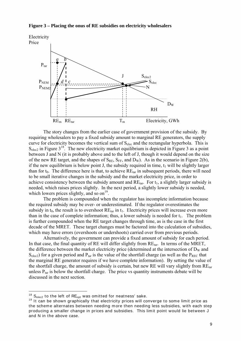
Figure 3 – Placing the onus of RE subsidies on electricity wholesalers Electricity Price a b Ptar J Selec2 PNEM d c Selec PNEM2 N DW RH REm REtar Tm Electricity, GWh The story changes from the earlier case of government provision of the subsidy. By requiring wholesalers to pay a fixed subsidy amount to marginal RE generators, the supply curve for electricity becomes the vertical sum of Selec and the rectangular hyperbola. This is Selec2 in Figure 318. The new electricity market equilibrium is depicted in Figure 3 as a point between J and N (it is probably above and to the left of J, though it would depend on the size of the new RE target, and the shapes of SRE, SFF, and DW). As in the scenario in Figure 2(b), if the new equilibrium is below point J, the subsidy required in time, t1 will be slightly larger than for t0. The difference here is that, to achieve REtar in subsequent periods, there will need to be small iterative changes in the subsidy and the market electricity price, in order to achieve consistency between the subsidy amount and REtar. For t1, a slightly larger subsidy is needed, which raises prices slightly. In the next period, a slightly lower subsidy is needed, which lowers prices slightly, and so on19.

The problem is compounded when the regulator has incomplete information because the required subsidy may be over- or underestimated. If the regulator overestimates the subsidy in t0, the result is to overshoot REtar in t1. Electricity prices will increase even more than in the case of complete information; thus, a lower subsidy is needed for t1. The problem is further compounded when the RE target changes through time, as is the case in the first decade of the MRET. These target changes must be factored into the calculation of subsidies, which may have errors (overshoots or undershoots) carried over from previous periods.

Alternatively, the government can provide a fixed amount of subsidy for each period. In that case, the final quantity of RE will differ slightly from REtar. In terms of the MRET, the difference between the market electricity price (determined at the intersection of DW and Selec2) for a given period and Ptar is the value of the shortfall charge (as well as the PREC that the marginal RE generator requires if we have complete information). By setting the value of the shortfall charge, the amount of subsidy is certain, but new RE will vary slightly from REtar unless Ptar is below the shortfall charge. The price vs quantity instruments debate will be discussed in the next section.

18 Selec2 to the left of REopt was omitted for neatness’ sake. 19 It can be shown graphically that electricity prices will converge to some limit price as the scheme alternates between needing more then needing less subsidies, with each step producing a smaller change in prices and subsidies. This limit point would lie between J and N in the above case.

10

A problem with Figure 3 is it assumes that any shortfall charge paid goes in full to marginal RE generators. This may not be the case in practise20 so that the rightward shift of SFF may be to the left (or to the right, for that matter) of REtar. This adds more uncertainty in determining the shape of Selec, and, hence, to determining actual NEM outcomes when the MRET is in place. JUSTIFYING TARGETS FOR RE

In practise, we cannot be certain of the benefits and costs of RE because of imperfect knowledge. SRE and SMCRE will both be within confidence intervals; in fact, all curves and values in Figures 1-3 are “expected” values. When there is uncertainty, REtar and the price effects of the subsidies are themselves “expected” values and we cannot be certain which instrument (price vs quantity instruments) will most likely result in REtar

21. In 1974, Weitzman published a seminal paper that sought to derive an “objective

criterion of the ceteris paribus advantage of a control mode [over another]” 22. He assumed quadratic Cost and Benefit functions of targeting a given commodity under uncertainty. He then investigated optimisation problems in which he maximised the expected difference between the benefits and costs, first, of using price instruments, then quantity instruments. By comparing the results of the respective maximisation problems, he derived an equation that describes the comparative advantage of price instruments over quantity instruments. He called this the “coefficient of comparative advantage”:

Eq.1

Where n, ρ, C′′ ≥ 0; B′′ ≤ 0; and σ2 is the mean square error in marginal cost.

A positive value for ∆n reveals an advantage for price instruments, while a negative value means an advantage for quantity instruments. It is worth noting Weitzman’s emphasis that this coefficient is merely a guide and qualitative data should not be left out of the decision-making process.

Comparative advantage is determined by four factors: - n – the number of generators of RE. As the number of generators increases, ∆n

increases, and the comparative advantage of prices goes up. - ρ – the correlation between marginal costs of different generators. ∆n increases as this

parameter increases. - C′′ - the second derivative of the cost function. As the cost function becomes more

curved, C′′ increases, making prices the better option. - B′′ - the second derivative of the benefit function. As the benefit function becomes

more curved, B′′ becomes more negative (we assume decreasing marginal benefit), decreasing ∆n giving quantity instruments greater comparative advantage.

Note: the above four conditions hold at the optimum solution.

The term, “Renewable Energy”, encompasses a host of different technologies (ie. wind, photovoltaics, bagasse, and so on). This naturally suggests low correlation between

20 Revenue from the shortfall charge may become general government revenue instead of RE subsidies. 21 When there is perfect knowledge, the use of price or quantity instruments are equivalent and lead to the same outcome. See Weitzman, M., “Prices vs. Quantities”, Review of Economic Studies, 41 (October, 1974) – p.480 22 See Weitzman for more detail.

( ) ( ) ⎥⎦

⎤⎢⎣

⎡⎟⎠⎞

⎜⎝⎛ +−+⎥

⎦

⎤⎢⎣

⎡+≈∆ ''''1

''21''''

''2 2

2

2

2

CBnC

CBCn

σρσρ

11

different generators’ cost structures. For example, many feel that wind energy is on the brink of commercial competitiveness, while photovoltaics are still expensive sources of electricity.

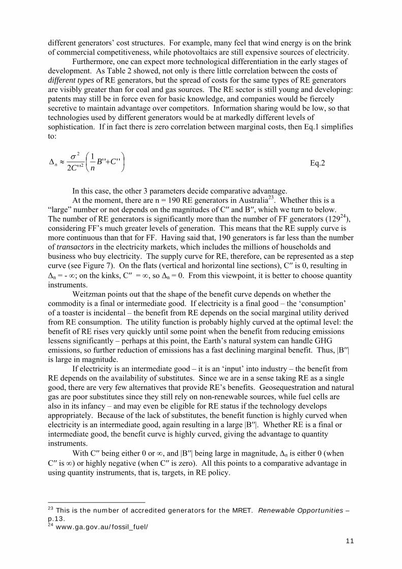
Furthermore, one can expect more technological differentiation in the early stages of development. As Table 2 showed, not only is there little correlation between the costs of different types of RE generators, but the spread of costs for the same types of RE generators are visibly greater than for coal and gas sources. The RE sector is still young and developing: patents may still be in force even for basic knowledge, and companies would be fiercely secretive to maintain advantage over competitors. Information sharing would be low, so that technologies used by different generators would be at markedly different levels of sophistication. If in fact there is zero correlation between marginal costs, then Eq.1 simplifies to:

Eq.2

In this case, the other 3 parameters decide comparative advantage.

At the moment, there are n = 190 RE generators in Australia23. Whether this is a “large” number or not depends on the magnitudes of C′′ and B′′, which we turn to below. The number of RE generators is significantly more than the number of FF generators (12924), considering FF’s much greater levels of generation. This means that the RE supply curve is more continuous than that for FF. Having said that, 190 generators is far less than the number of transactors in the electricity markets, which includes the millions of households and business who buy electricity. The supply curve for RE, therefore, can be represented as a step curve (see Figure 7). On the flats (vertical and horizontal line sections), C′′ is 0, resulting in ∆n = - ∞; on the kinks, C′′ = ∞, so ∆n = 0. From this viewpoint, it is better to choose quantity instruments. Weitzman points out that the shape of the benefit curve depends on whether the commodity is a final or intermediate good. If electricity is a final good – the ‘consumption’ of a toaster is incidental – the benefit from RE depends on the social marginal utility derived from RE consumption. The utility function is probably highly curved at the optimal level: the benefit of RE rises very quickly until some point when the benefit from reducing emissions lessens significantly – perhaps at this point, the Earth’s natural system can handle GHG emissions, so further reduction of emissions has a fast declining marginal benefit. Thus, |B′′| is large in magnitude. If electricity is an intermediate good – it is an ‘input’ into industry – the benefit from RE depends on the availability of substitutes. Since we are in a sense taking RE as a single good, there are very few alternatives that provide RE’s benefits. Geosequestration and natural gas are poor substitutes since they still rely on non-renewable sources, while fuel cells are also in its infancy – and may even be eligible for RE status if the technology develops appropriately. Because of the lack of substitutes, the benefit function is highly curved when electricity is an intermediate good, again resulting in a large |B′′|. Whether RE is a final or intermediate good, the benefit curve is highly curved, giving the advantage to quantity instruments.

With C′′ being either 0 or ∞, and |B′′| being large in magnitude, ∆n is either 0 (when C′′ is ∞) or highly negative (when C′′ is zero). All this points to a comparative advantage in using quantity instruments, that is, targets, in RE policy.

23 This is the number of accredited generators for the MRET. Renewable Opportunities – p.13. 24 www.ga.gov.au/fossil_fuel/

⎟⎠⎞

⎜⎝⎛ +≈∆ ''''1

''2 2

2

CBnCn

σ

12

SECTION II THE ECONOMICS OF MRET – REC Markets and the Shortfall Charge RECs

Each MWh of electricity generated from eligible plants installed after 1997 is able to create one REC. For plants installed prior to 1997, RECs can be created for every MWh produced above a pre-calculated baseline (see Appendix 4 for eligible RE sources). Once created, wholesalers can obtain RECs from owners of existing RECs – including generators, other liable parties, or even speculators. Of course, wholesalers purchasing electricity directly from RE generators can include the provision of RECs as part of the contract. There is no formal market for RECs, though the Office of the Renewable Energy Regulator (ORER) maintains a website that records and keeps track of all available RECs to facilitate trade. On February 14 of each year, liable parties surrender an amount of RECs equivalent to their past year’s RPP25, or pay the shortfall charge.

RECs are a premium on top of the price RE generators receive from electricity markets. If the average electricity price in the NEM is $35-40, Table 1 tells us that most RE sources are not competitive without such a premium. Ideally, the price of RECs should, along with the NEM price, cover the costs of the last generator needed for the year’s target.

Let us now model the actual NEM. Prior to the MRET, we get an outcome similar to the market conditions in Figure 4, which reproduces the market aspects of Figure 1, but with non-linear curves to better represent reality. Remember that equilibrium was at point J, where we have total electricity supply of Tm in the quoted price range of $35-40. Conventional generators supply FFm, while RE supply REm, which is equivalent to RE’s 9.9% contribution to total electricity discussed earlier. Figure 4 – The electricity market in 2000 (without MRET) Electricity Price SRE(2000) SFF ST A $35-40 J DW REm FFm Tm Electricity, GWh The MRET forces the quantity of RE supplied to increase from REm to RE2001 once the MRET begins. From Table 1, we know that the target for 2001 is an extra 300GWh of RE. This allows more costly RE to enter the market at the expense of some FF. The effect on prices depends on the shapes of the supply and demand curves for the years 2000, and 2001. Assuming there are no shifts, electricity prices will depend on Selec and the size of the subsidy. Because RE is such a small part of the market, the increase in price is likely to be small. One 25 “Renewable Energy Certificates Fact Sheet” – www.orer.gov.au/factsheets/certificates.html

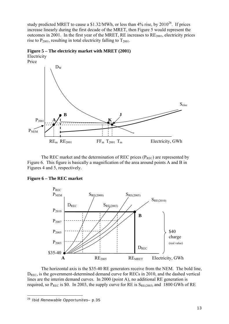
13

study predicted MRET to cause a $1.32/MWh, or less than 4% rise, by 201026. If prices increase linearly during the first decade of the MRET, then Figure 5 would represent the outcomes in 2001. In the first year of the MRET, RE increases to RE2001, electricity prices rise to P2001, resulting in total electricity falling to T2001. Figure 5 – The electricity market with MRET (2001) Electricity Price DW Selec B J P2001 A K PNEM REm RE2001 FFm T2001 Tm Electricity, GWh

The REC market and the determination of REC prices (PREC) are represented by Figure 6. This figure is basically a magnification of the area around points A and B in Figures 4 and 5, respectively. Figure 6 – The REC market PREC PNEM SRE(2000) SRE(2005) SRE(2010) DREC SRE(2003) P2010 B P2007 P2005 $40

charge P2003 (real value) DREC $35-40 A RE2005 REMRET Electricity, GWh The horizontal axis is the $35-40 RE generators receive from the NEM. The bold line, DREC, is the government-determined demand curve for RECs in 2010, and the dashed vertical lines are the interim demand curves. In 2000 (point A), no additional RE generation is required, so PREC is $0. In 2003, the supply curve for RE is SRE(2003) and 1800 GWh of RE

26 Ibid Renewable Opportunites– p.35

14

generation is mandated, so the REC price required for the last RE generator to enter the market is P2003.

RE technology is continually developing, and this should receive a boost as revenue from RECs, as well as government schemes like Backing Australia’s Ability is directed towards R&D27. The RE supply is continually shifting rightward, as depicted in Figure 6 by the shift from SRE(2000) to SRE(2003) by 2003, then to SRE(2005) by 2005, and so on. The diagram predicts a gradual increase in PREC until 2010, when it would be equal to or less than the $40/MWh shortfall charge. The Shortfall Charge (SFC)

The value of the SFC was derived with the objective of encouraging the purchase of RECs. If a liable party chooses to pay the penalty as a result of not delivering RECs, his cost becomes $40/MWh + $35-40 from the NEM. As we saw earlier, buying energy from RE sources costs him PREC + $35-40 from the NEM. To encourage REC purchase, we must have

$40/MWh + $35-40 ≥ PREC + $35-40; OR $40/MWh ≥ PREC

which is what Figure 6 depicts. There are two factors that can increase the effective value of the SFC and, hence,

widen the number of RE generators that benefit from MRET: 1) The $40/MWh penalty is not tax-deductible, so companies may be indifferent between

paying the penalty and paying as much as $57 per REC, depending on whether or not shareholders can fully utilise the tax credit for franked dividends (see Appendix 5).

2) The names of parties who pay the shortfall charge are mentioned in a yearly “shame list” published by ORER. Parties sensitive to such matters may be willing buy RECs for more than $40/$57.

Under the strict $40/MWh SFC, co-firing biomass, bagasse, small-scale hydro, landfill

gas, and solar hot water are the RE sources mentioned in Table 1 that benefit. When the two aforementioned factors are considered, the list widens to include biomass, agricultural biogas, municipal waste, and the more efficient of the grid-connected wind generators.

Figures 4-6 obviously model only the basic principles of MRET. We now look at

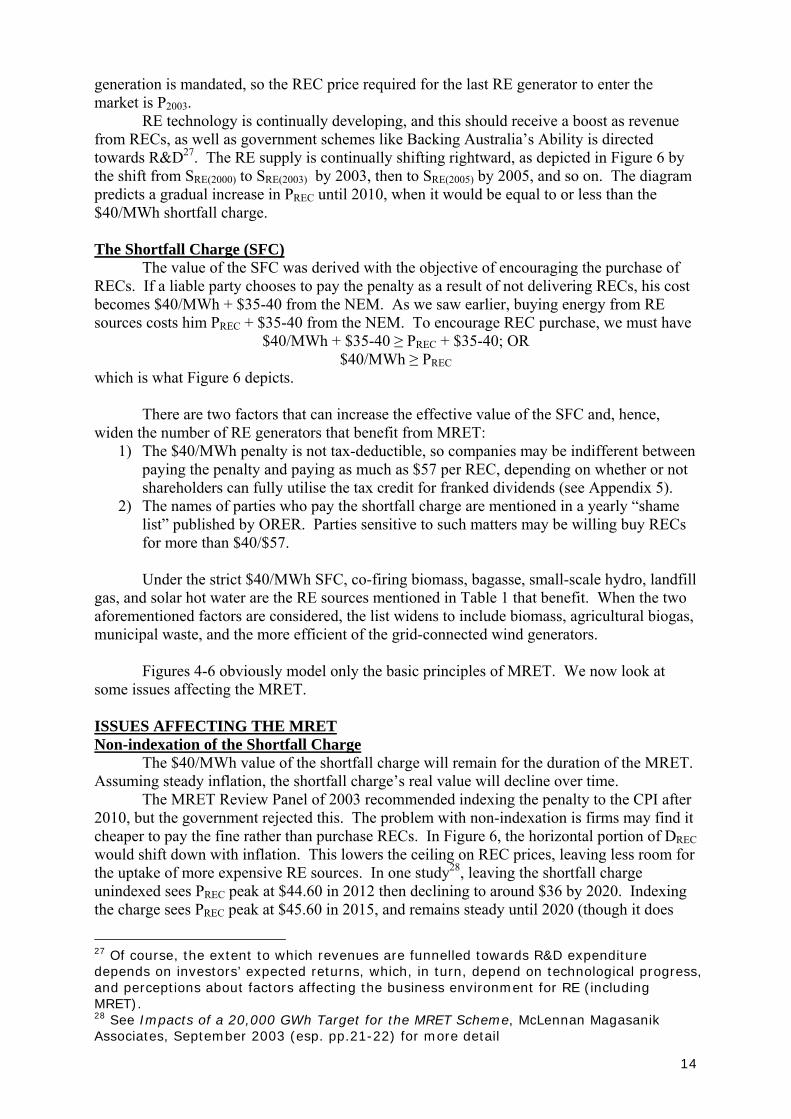
some issues affecting the MRET. ISSUES AFFECTING THE MRET Non-indexation of the Shortfall Charge The $40/MWh value of the shortfall charge will remain for the duration of the MRET. Assuming steady inflation, the shortfall charge’s real value will decline over time.

The MRET Review Panel of 2003 recommended indexing the penalty to the CPI after 2010, but the government rejected this. The problem with non-indexation is firms may find it cheaper to pay the fine rather than purchase RECs. In Figure 6, the horizontal portion of DREC would shift down with inflation. This lowers the ceiling on REC prices, leaving less room for the uptake of more expensive RE sources. In one study28, leaving the shortfall charge unindexed sees PREC peak at $44.60 in 2012 then declining to around $36 by 2020. Indexing the charge sees PREC peak at $45.60 in 2015, and remains steady until 2020 (though it does

27 Of course, the extent to which revenues are funnelled towards R&D expenditure depends on investors’ expected returns, which, in turn, depend on technological progress, and perceptions about factors affecting the business environment for RE (including MRET). 28 See Impacts of a 20,000 GWh Target for the MRET Scheme, McLennan Magasanik Associates, September 2003 (esp. pp.21-22) for more detail

15

fall slightly due to decreasing costs in RE technology). Indexing thus gives the RE industry more support.

Proponents of no indexation argue that it would put more pressure on RE generators to increase efficiency, so they can derive the most benefit out of REC revenues, and to stay in the market longer.

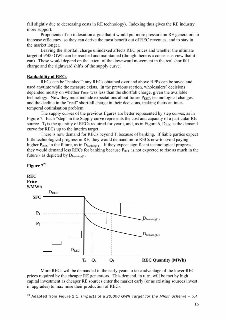
Leaving the shortfall charge unindexed affects REC prices and whether the ultimate target of 9500 GWh can be reached and maintained (though there is a consensus view that it can). These would depend on the extent of the downward movement in the real shortfall charge and the rightward shifts of the supply curve. Bankability of RECs RECs can be “banked”: any RECs obtained over and above RPPs can be saved and used anytime while the measure exists. In the previous section, wholesalers’ decisions depended mostly on whether PREC was less than the shortfall charge, given the available technology. Now they must include expectations about future PREC, technological changes, and the decline in the “real” shortfall charge in their decisions, making theirs an inter-temporal optimisation problem.

The supply curves of the previous figures are better represented by step curves, as in Figure 7. Each “step” in the Supply curve represents the cost and capacity of a particular RE source. Ti is the quantity of RECs required for year i, and, as in Figure 6, DREC is the demand curve for RECs up to the interim target.

There is now demand for RECs beyond Ti because of banking. If liable parties expect little technological progress in RE, they would demand more RECs now to avoid paying higher PREC in the future, as in Dbanking(1). If they expect significant technological progress, they would demand less RECs for banking because PREC is not expected to rise as much in the future - as depicted by Dbanking(2). Figure 729 REC Price $/MWh DREC SFC

P1 Dbanking(1) P2 Dbanking(2) DREC Ti Q2 Q1 REC Quantity (MWh) More RECs will be demanded in the early years to take advantage of the lower REC prices required by the cheaper RE generators. This demand, in turn, will be met by high capital investment as cheaper RE sources enter the market early (or as existing sources invest in upgrades) to maximise their production of RECs. 29 Adapted from Figure 2.1, Impacts of a 20,000 GWh Target for the MRET Scheme – p.4

16

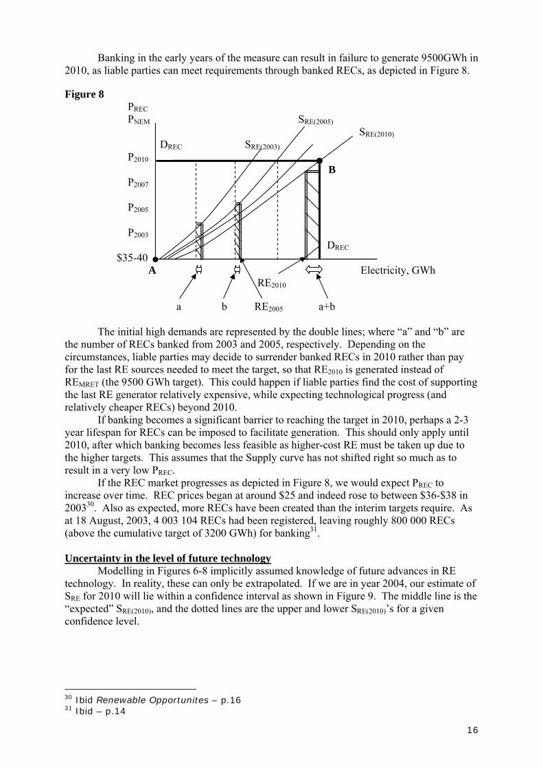
Banking in the early years of the measure can result in failure to generate 9500GWh in 2010, as liable parties can meet requirements through banked RECs, as depicted in Figure 8. Figure 8 PREC PNEM SRE(2005) SRE(2010) DREC SRE(2003) P2010 B P2007 P2005

P2003 DREC $35-40 A Electricity, GWh

RE2010 a b RE2005 a+b

The initial high demands are represented by the double lines; where “a” and “b” are the number of RECs banked from 2003 and 2005, respectively. Depending on the circumstances, liable parties may decide to surrender banked RECs in 2010 rather than pay for the last RE sources needed to meet the target, so that RE2010 is generated instead of REMRET (the 9500 GWh target). This could happen if liable parties find the cost of supporting the last RE generator relatively expensive, while expecting technological progress (and relatively cheaper RECs) beyond 2010.

If banking becomes a significant barrier to reaching the target in 2010, perhaps a 2-3 year lifespan for RECs can be imposed to facilitate generation. This should only apply until 2010, after which banking becomes less feasible as higher-cost RE must be taken up due to the higher targets. This assumes that the Supply curve has not shifted right so much as to result in a very low PREC.

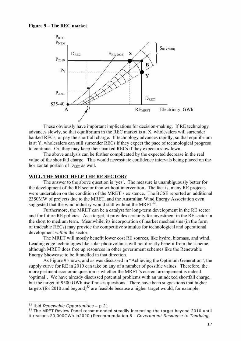
If the REC market progresses as depicted in Figure 8, we would expect PREC to increase over time. REC prices began at around $25 and indeed rose to between $36-$38 in 200330. Also as expected, more RECs have been created than the interim targets require. As at 18 August, 2003, 4 003 104 RECs had been registered, leaving roughly 800 000 RECs (above the cumulative target of 3200 GWh) for banking31. Uncertainty in the level of future technology Modelling in Figures 6-8 implicitly assumed knowledge of future advances in RE technology. In reality, these can only be extrapolated. If we are in year 2004, our estimate of SRE for 2010 will lie within a confidence interval as shown in Figure 9. The middle line is the “expected” SRE(2010), and the dotted lines are the upper and lower SRE(2010)’s for a given confidence level.

30 Ibid Renewable Opportunites – p.16 31 Ibid – p.14

17

Figure 9 – The REC market PREC PNEM SRE(2010) DREC SRE(2003) X P2010 B PY Y P2003 DREC $35-40 A REMRET Electricity, GWh a These obviously have important implications for decision-making. If RE technology advances slowly, so that equilibrium in the REC market is at X, wholesalers will surrender banked RECs, or pay the shortfall charge. If technology advances rapidly, so that equilibrium is at Y, wholesalers can still surrender RECs if they expect the pace of technological progress to continue. Or, they may keep their banked RECs if they expect a slowdown. The above analysis can be further complicated by the expected decrease in the real value of the shortfall charge. This would necessitate confidence intervals being placed on the horizontal portion of DREC as well. WILL THE MRET HELP THE RE SECTOR?

The answer to the above question is ‘yes’. The measure is unambiguously better for the development of the RE sector than without intervention. The fact is, many RE projects were undertaken on the condition of the MRET’s existence. The BCSE reported an additional 2350MW of projects due to the MRET, and the Australian Wind Energy Association even suggested that the wind industry would stall without the MRET32.

Furthermore, the MRET can be a catalyst for long-term development in the RE sector and for future RE policies. As a target, it provides certainty for investment in the RE sector in the short to medium term. Meanwhile, its incorporation of market mechanisms (in the form of tradeable RECs) may provide the competitive stimulus for technological and operational development within the sector. The MRET will mostly benefit lower cost RE sources, like hydro, biomass, and wind. Leading edge technologies like solar photovoltaics will not directly benefit from the scheme, although MRET does free up resources in other government schemes like the Renewable Energy Showcase to be funnelled in that direction. As Figure 9 shows, and as was discussed in “Achieving the Optimum Generation”, the supply curve for RE in 2010 can take on any of a number of possible values. Therefore, the more pertinent economic question is whether the MRET’s current arrangement is indeed ‘optimal’. We have already discussed potential problems with an unindexed shortfall charge, but the target of 9500 GWh itself raises questions. There have been suggestions that higher targets (for 2010 and beyond)33 are feasible because a higher target would, for example,

32 Ibid Renewable Opportunities – p.21 33 The MRET Review Panel recommended steadily increasing the target beyond 2010 until it reaches 20,000GWh in2020 (Recommendation 8 - Government Response to Tambling

18

achieve economies of scale in RE generation. Because of these uncertainties, periodic reviews of the target may be warranted; however, these would incur extra costs, and create more uncertainties! Efficiency, Gainers, and Losers So, who wins and who loses from the MRET? As mentioned in the previous section, RE up to the marginal generator gain producer surplus from the subsidies. FF generators pay some of the costs of GHG externalities through reduced generation, but they do not pay the optimal amount because the costs are spread throughout the NEM. Furthermore, REtar may be less than the optimal target, leading to even lower taxes for FF. Meanwhile, higher electricity prices mean a loss of consumer surplus (or a loss in profits for commercial users of electricity). From a strict efficiency point of view, placing a tax on FF generators (L-M in Figure 1) or imposing quantitative restrictions combined with marketable permits should lead to the optimal outcome. Subsidies are unnecessary if indeed RE does not have any positive externalities.

Subsidies, however, are advantageous in that they provide temporary stimulus to R&D and investment in RE. From the government’s point of view, this signals a more direct commitment to alternative fuels than the single tax on FF. Assuming that REtar ignores overseas emissions costs, providing subsidies via the MRET scheme would also place less imposition on electricity users, all at no cost to the budget. Appendix 1 – Share of RE in Total Electricity Generation, 1996-9734

State RE Generated (GWh) % Share of RE in Total Electricity

NSW 5,341 8.3 Victoria 1,396 3.2 Queensland 1,482 4.0 South Australia 28 0.4 Western Australia 202 1.1 Tasmania 9,739 99.6 Northern Territory 1 0.00 Australia 18,189 9.9 Appendix 2 – The Basics of Global Warming Approximately 22% of solar radiation approaching the Earth is absorbed by clouds35. The rest of the radiation travel to the Earth’s surface, where it is reflected off light surfaces like snow, or it is absorbed by land, water, or vegetation; much of this absorbed energy is then re-radiated towards outer space (mostly in the form of infrared rays). However, a small portion of this energy is re-absorbed by Greenhouse Gases in the atmosphere, particularly carbon dioxide, methane, and nitrous oxide, as well as water vapour. Thus, it is incoming solar energy as well as reradiated, but GHG-absorbed energy that give the Earth’s surface it’s relatively warm surface temperature.

Mandatory Renewable Energy Target (MRET) Review Recommendations, Australian Greenhouse Office) 34 www.abs.gov.au/Websitedbs/c311215.nsf/0/E2D569D2A2D40505CA2569E7000ACB5?Open 35 Hussen, A.M., Principles of Environmental Economics, Routledge, New York, 2000 – p.272

19

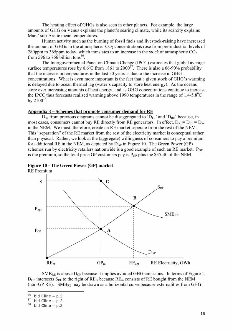
The heating effect of GHGs is also seen in other planets. For example, the large amounts of GHG on Venus explains the planet’s searing climate, while its scarcity explains Mars’ sub-Arctic mean temperatures. Human activity such as the burning of fossil fuels and livestock-raising have increased the amount of GHGs in the atmosphere. CO2 concentrations rose from pre-industrial levels of 280ppm to 365ppm today, which translates to an increase in the stock of atmospheric CO2 from 596 to 766 billion tons36. The Intergovernmental Panel on Climate Change (IPCC) estimates that global average surface temperatures rose by 0.60C from 1861 to 200037. There is also a 66-90% probability that the increase in temperatures in the last 50 years is due to the increase in GHG concentrations. What is even more important is the fact that a given stock of GHG’s warming is delayed due to ocean thermal lag (water’s capacity to store heat energy). As the oceans store ever increasing amounts of heat energy, and as GHG concentrations continue to increase, the IPCC thus forecasts realised warming above 1990 temperatures in the range of 1.4-5.80C by 210038. Appendix 3 – Schemes that promote consumer demand for RE

DW from previous diagrams cannot be disaggregated to ‘DFF’ and ‘DRE’ because, in most cases, consumers cannot buy RE directly from RE generators. In effect, DRE= DFF = DW in the NEM. We must, therefore, create an RE market seperate from the rest of the NEM. This “separation” of the RE market from the rest of the electricity market is conceptual rather than physical. Rather, we look at the (aggregate) willingness of consumers to pay a premium for additional RE in the NEM, as depicted by DGP in Figure 10. The Green Power (GP) schemes run by electricity retailers nationwide is a good example of such an RE market. PGP is the premium, so the total price GP customers pay is PGP plus the $35-40 of the NEM. Figure 10 - The Green Power (GP) market RE Premium S C SRE B Popt SMBRE PGP A DGP REm GPm REopt RE Electricity, GWh SMBRE is above DGP because it implies avoided GHG emissions. In terms of Figure 1, DGP intersects SRE to the right of REm because REm consists of RE bought from the NEM (non-GP RE). SMBRE may be drawn as a horizontal curve because externalities from GHG 36 Ibid Cline – p.2 37 Ibid Cline – p.2 38 Ibid Cline – p.2

20

emissions have a global dimension. The decrease in marginal benefit (to the world) from each additional RE generated in Australia will be very small, though we do not look at that case here39.

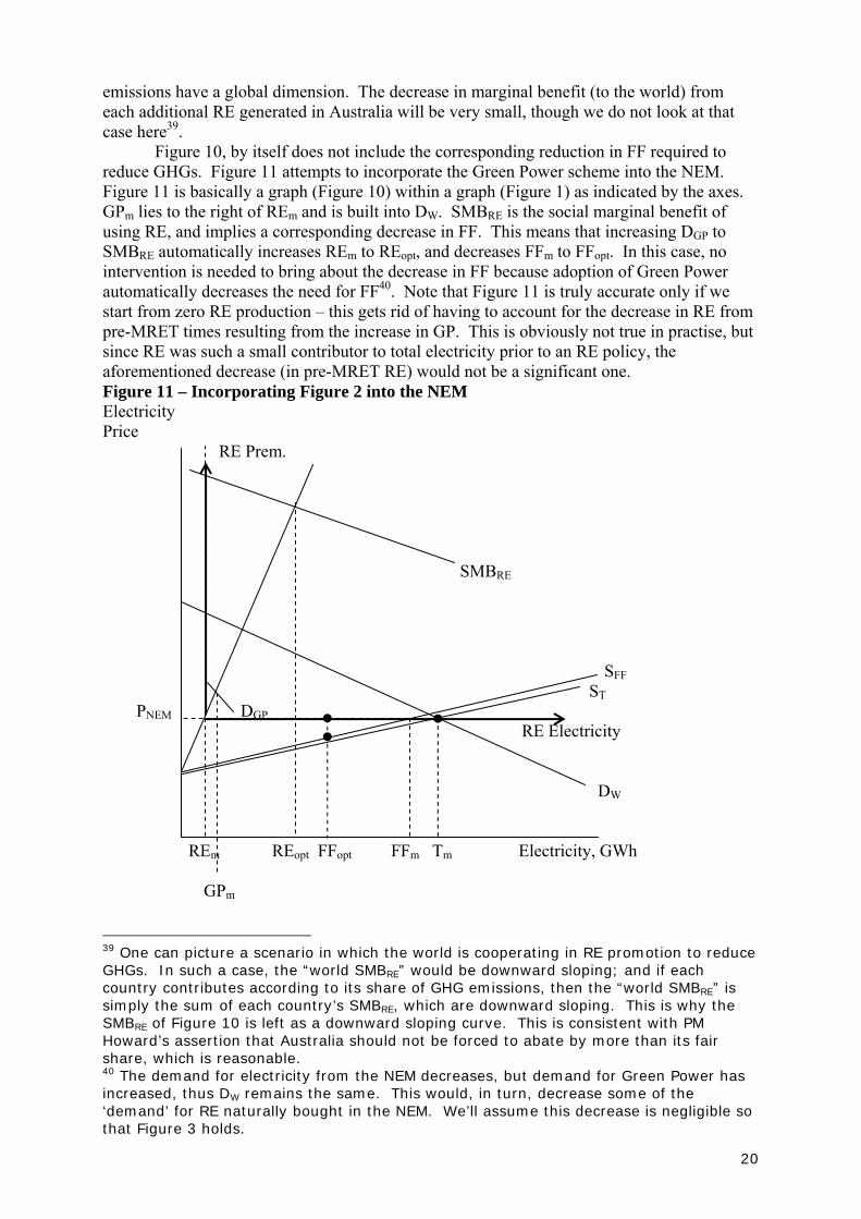
Figure 10, by itself does not include the corresponding reduction in FF required to reduce GHGs. Figure 11 attempts to incorporate the Green Power scheme into the NEM. Figure 11 is basically a graph (Figure 10) within a graph (Figure 1) as indicated by the axes. GPm lies to the right of REm and is built into DW. SMBRE is the social marginal benefit of using RE, and implies a corresponding decrease in FF. This means that increasing DGP to SMBRE automatically increases REm to REopt, and decreases FFm to FFopt. In this case, no intervention is needed to bring about the decrease in FF because adoption of Green Power automatically decreases the need for FF40. Note that Figure 11 is truly accurate only if we start from zero RE production – this gets rid of having to account for the decrease in RE from pre-MRET times resulting from the increase in GP. This is obviously not true in practise, but since RE was such a small contributor to total electricity prior to an RE policy, the aforementioned decrease (in pre-MRET RE) would not be a significant one. Figure 11 – Incorporating Figure 2 into the NEM Electricity Price RE Prem.

SMBRE SFF ST PNEM DGP RE Electricity DW REm REopt FFopt FFm Tm Electricity, GWh

GPm 39 One can picture a scenario in which the world is cooperating in RE promotion to reduce GHGs. In such a case, the “world SMBRE” would be downward sloping; and if each country contributes according to its share of GHG emissions, then the “world SMBRE” is simply the sum of each country’s SMBRE, which are downward sloping. This is why the SMBRE of Figure 10 is left as a downward sloping curve. This is consistent with PM Howard’s assertion that Australia should not be forced to abate by more than its fair share, which is reasonable. 40 The demand for electricity from the NEM decreases, but demand for Green Power has increased, thus DW remains the same. This would, in turn, decrease some of the ‘demand’ for RE naturally bought in the NEM. We’ll assume this decrease is negligible so that Figure 3 holds.

21

Note that there is a correspondence between SMCFF and SMBRE. The steeper the former is, the flatter the latter becomes. A steep SMCFF means that decreasing FF greatly decreases its social marginal costs. Thus, increasing RE results in a lower decrease in its social marginal benefits. In order to get RE generation up to REopt, consumers can be subsidised the value, S – PGP, per unit of new RE. But SMBRE is probably much further out than indicated, so the cost of subsidies may be enormous.

A better solution is to increase public awareness of RE and its benefits, which is low at this stage. This would shift DGP rightwards as more people become willing to pay a premium for RE. Of course, increasing awareness of RE will not necessarily translate to a shift in DRE. In surveys, consumers often reveal that they are willing to pay a premium for RE. Whether or not they actually subscribe to Green Power schemes is another matter. The benefits from RE are non-rival and non-excludable, so there is an incentive to free-ride. This is exacerbated by the inter-temporal aspect of global warming because the problem seems less urgent to today’s populations. Changing people’s demands may require considerably more investment (money and time) than directly subsidizing new RE generators. Appendix 4 – Eligible Renewable Energy Sources41

The following technologies/sources will be eligible under the measure (where used for electricity generation, or in the case of solar hot water, where displacing electricity):

• hydro;

• wind;

• solar;

• bagasse co-generation;

• black liquor;

• wood waste;

• energy crops;

• crop waste;

• food and agricultural wet waste;

• landfill gas;

• municipal solid waste combustion;

• sewage gas;

• geothermal-aquifer;

• tidal;

• photovoltaic and photovoltaic Renewable Stand Alone Power Supply systems;

• wind and wind hybrid Renewable Stand Alone Power Supply systems;

• micro hydro Renewable Stand Alone Power Supply systems;

• solar hot water;

• co-firing; 41 Ibid “Overview of the Mandatory Renewable Energy Target” – www.orer.gov.au/overview.html

22

• wave;

• ocean;

• fuel cells;

• hot dry rocks.

Notes and Qualifications: As appropriate, developments or projects will be subject to local environmental requirements/regulation. Where electricity is produced from a combination of renewable and fossil fuel energy, the fossil fuel contribution will be netted out. Solar water heaters can be included where the installation leads to a positive greenhouse gas benefit and where the fossil fuel contribution is netted out. Fossil fuel electricity consumption in pump storage hydro will be netted out. Renewable installations off-grid will also be eligible to contribute towards meeting the target (ie eligibility is not determined by grid).

Fossil fuels and fossil fuel derived waste products will not be eligible under this measure, including:

• coal seam methane, waste coal mine gas and other coal or natural gas based products;

• waste heat from cogeneration;

• electricity production from cogeneration based on fossil fuels;

• non-biomass component of co-firing or wastes. Appendix 5 – The $40/MWh Shortfall Charge42 The value of the penalty is determined from the viewpoint of the shareholder. If shareholders can fully utilise the tax credit for franked dividends, the income available to the shareholder, before personal tax is:

(1-0.3)P + 0.3P = P

where, P = the company’s net profit before tax 0.3 = the corporate tax rate If the shareholder cannot use the franking credits, his pre-tax income is:

(1-0.3)P If the shareholder can use franking credits in between the above “extremes”, his pre-tax income is:

(1-0.3)P + γ0.3P = [1-(1-γ)0.3]P

γ represents the extent to which franking credits can be used. γ=1 means full use of franking credits, while γ=0 means they cannot be used. If the company must (or chooses to) pay the shortfall charge, the effective income to shareholders is:

(1-0.3)P + γ0.3P - 40

42 Ibid (IES)– p.19-20

23

Now, let pREC be the (tax deductible) price of RECs that is equivalent to the shortfall charge:

(1-0.3)P + γ0.3P – 40 = (1-0.3)(P-pREC) + γ0.3(P-pREC) 40 = (1-0.3)pREC + γ0.3pREC pREC = 40/[(1-0.3) + γ0.3]

pREC = 40/[1-(1- γ)0.3] When γ=0, the equivalent pREC is 40/0.7 = $57 When γ=0.5, the equivalent pREC is 40/0.85 = $47 When γ=1, the equivalent pREC is 40/1 = $40 Note that regulators like the ACCC have used γ=0.5 in the past when looking into regulations into the electricity industry. REFERENCES Cline, W.R., “Meeting the Challenge of Global Warming”, Copenhagen Consensus Challenge Paper, 2004 Gottliebsen, R., “Insurers raise the eco-alarm”, The Weekend Australian, September 4-5, 2004 Hussen, A.M., Principles of Environmental Economics, Routledge, New York, 2000 Weitzman, M., “Prices vs. Quantities”, Review of Economic Studies 41 (October 1974) Young, BC, & Allardice, DJ, The Implementation of the 2% Mandatory Renewable Energy Target in Australia, A study commissioned by New Energy and Industrial Technology Development Organisation (NEDO), March 2001 An Introduction to Australia’s National Electricity Market, NEMMCO, June 2004 Government Response to Tambling Mandatory Renewable Energy Target (MRET) Review Recommendations, Australian Greenhouse Office Impacts of a 20,000 GWh Target for the MRET Scheme, McLennan Magasanik Associates, September 2003 Key Issues in Developing Renewables, International Energy Agency, 1997 “Overview of the Mandatory Renewable Energy Target” – www.orer.gov.au/overview.html “Renewable Energy Certificates Fact Sheet” – www.orer.gov.au/factsheets/certificates.html Renewable Opportunites: A Review of the Renewable Energy (Electricity) Act 2000, September 2003, Australian Greenhouse Office Securing Australia’s Energy Future, Commonwealth of Australia, 2004 World Energy Outlook 1998 Edition, International Energy Agency www.abs.gov.au/Ausstats/abs%40.nsf/94713ad445ff1425ca25682000192af2/738488bd76f41498ca256dea00053964!OpenDocument [1]

24

www.abs.gov.au/Websitedbs/c311215.nsf/0/E2D569D2A2D40505CA2569E7000ACB5?Open [2] www.ga.gov.au/fossil_fuel/