MNRAS 431, 240–251 (2013) doi:10.1093/mnras/stt158Advance Access publication 2013 March 07

The Edinburgh–Cape Blue Object Survey – III. Zone 2; galactic latitudes−30◦ > b > −40◦

D. O’Donoghue,1,2 D. Kilkenny,3‹ C. Koen,4 N. Hambly,5 H. MacGillivray5

and R. S. Stobie1

1South African Astronomical Observatory, PO Box 9, Observatory 7935, South Africa2The Southern African Large Telescope, PO Box 9, Observatory 7935, South Africa3Department of Physics, University of the Western Cape, Private Bag X17, Bellville 7535, South Africa4Department of Statistics, University of the Western Cape, Private Bag X17, Bellville 7535, South Africa5Wide Field Astronomy Unit, Institute for Astronomy, University of Edinburgh, Blackford Hill, Edinburgh EH9 3HJ, UK

Accepted 2013 January 24. Received 2013 January 24; in original form 2012 December 20

ABSTRACTThe Edinburgh–Cape Blue Object Survey seeks to identify point sources with an ultravioletexcess. Results for zone 2 of the survey are presented here, covering that part of the SouthGalactic Cap between 30◦ and 40◦ from the Galactic plane and south of about −12.◦3 ofdeclination. Edinburgh–Cape zone 2 comprises 66 UK Schmidt Telescope fields coveringabout 1730 deg2, in which we find some 892 blue objects, including 423 hot subdwarfs(∼47 per cent); 128 white dwarfs (∼14 per cent); 25 cataclysmic variables (∼3 per cent); 119binaries (∼13 per cent), mostly composed of a hot subdwarf and a main-sequence F or G star;66 horizontal branch stars (∼7 per cent) and 48 ‘star-like’ extragalactic objects (∼5 per cent).A further 362 stars observed in the survey, mainly low-metallicity F- and G-type stars, are alsolisted. Both low-dispersion spectroscopic classification and UBV photometry are presented foralmost all of the hot objects and either spectroscopy or photometry (or both) for the coolerones.

Key words: surveys – stars: early-type – stars: horizontal branch – subdwarfs – white dwarfs –quasars: general.

1 IN T RO D U C T I O N

Historically – and until relatively recently – most of the astronomi-cal observatories, and most of the astronomers, have been located inthe Northern hemisphere. This has resulted in a north–south imbal-ance in the numbers of catalogued objects, including the ‘faint bluestars’. From the earliest systematic surveys (Humason & Zwicky1947), it was realized that these objects were not a homogenousgroup and that the stars were generally subluminous relative tomain-sequence stars of the same colour. Among this loose group-ing, we now recognize white dwarfs, horizontal branch stars, hotsubdwarf stars, cataclysmic variables (CVs) and even quasars. Butthe earliest surveys were substantially Northern hemisphere (onecannot consider this subject without thinking immediately of theextensive work done by Luyten over decades – see Luyten 1953,1954, 1969; Haro & Luyten 1962, as examples) and even the morerecent surveys such as the Palomar–Green (PG) survey (Green,Schmidt & Liebert 1986) and the overwhelming Sloan Digital SkySurvey (Abazajian et al. 2003) have been effectively northern.

� E-mail: dkilkenny@uwc.ac.za

An illustration of the effect this has had on the availability ofsouthern research material is given by the pulsating white dwarfstars. Prior to the Sloan Digital Sky Survey (SDSS), out of approx-imately 80 known DA pulsators (DAV or ZZ Ceti stars) only abouta quarter are in the Southern hemisphere – and many of those areequatorial. This imbalance has not significantly improved with newresults – see Mukadam et al. (2004) and Mullally et al. (2005).Before the Sloan survey, of the nine known DB pulsators (DBV orV777 Her stars) only one is southern – and that was discovered bythe Edinburgh–Cape (EC) survey (Koen et al. 1995). Nitta et al.(2009) doubled the number of known DBV stars but naturally thenew SDSS discoveries are mainly northern. Of the five known DOpulsators (DOV or GW Vir stars), only the prototype, PG 1159−034itself, is southern – and that was found by the northern PG survey.

A principal motivation behind the EC survey was thus to correctthe very evident imbalance between the numbers of hot, interestingobjects known to exist in the northern and southern hemispheres;in short, we wanted more southern sources for detailed study. Fromthe outset, it was hoped that the EC survey would prove as suc-cessful in the south as the comparable PG survey has been in thenorth.

In the absence of any excess of modesty, we can claim severalsuccesses for the EC survey, including the following.

C© 2013 The AuthorsPublished by Oxford University Press on behalf of the Royal Astronomical Society

Edinburgh–Cape Survey: Zone 2 241

(i) Publication of a description of the survey (Stobie et al. 1997b,hereafter Paper I) together with the first EC zone – the North Galac-tic Cap south of declination −12.◦5 (Kilkenny et al. 1997b, here-after Paper II). The latter covered about 1560 deg2 and containedsome 955 objects brighter than B = 16.5 mag, of which 675 weregenuinely hot (comparable to OB stars in temperature) and theremainder were F- or G-type stars.

(ii) The discovery of the first rapidly pulsating sdB stars(Kilkenny et al. 1997a; Koen et al. 1997; O’Donoghue et al. 1997;Stobie et al. 1997a). This led directly to a more widespread searchfor sdB pulsators among the survey stars and elsewhere, resulting inthe discovery of several new pulsators, including PG 1605+072, alarge-amplitude, multifrequency, evolved sdB pulsator (Koen et al.1998), and PG 1336−018, the first sdB pulsator to be found in aneclipsing binary system (Kilkenny et al. 1998b).

(iii) The discovery of a number of unusual and rare objects, in-cluding the spectacular eclipsing DA+dM binary, EC 13471−1256(O’Donoghue et al. 2003), in which the cool companion exhibitssignificant flares. A new member of the class of rare AM CVnvariables was found (O’Donoghue et al. 1994) as were several newmembers of the rare pulsating DB white dwarf stars (Koen et al.1995; Kilkenny et al. 2009).

(iv) Studies of selected classes of object have been carried out.Chen et al. (2001) reported work on new CVs found in the EC surveyand a multiwavelength study was made of EC objects with essen-tially featureless spectra in the optical region (Sefako et al. 1999).A study of a significant sample of low-metallicity F- and G-typestars was carried out by Beers et al. (2001) and the apparently nor-mal B stars found in the survey were resolved into post-asymptoticgiant branch (AGB) stars (Lynn et al. 2005) and normal B stars atlarge distances from the Galactic plane (Magee et al. 2001; Lynnet al. 2004), which were additionally used to study the interstellarmedium via the Ca II K line (Smoker et al. 2003).

2 SU RV E Y PL A N

The EC survey plan and the methods employed were laid out inconsiderable detail in Paper I. However, since that paper was written,some changes have been forced on to the survey for several disparatereasons, described in this section and the next.

A significant change is that the original survey was planned tocover the whole of the southern sky which had a Galactic latitude|b| > 30◦. This would have involved obtaining nearly 400 Schmidtplate pairs covering almost 10 000 deg2. Early in the project, itwas realized that this would be a massive undertaking – and wouldoverlap substantially with the southern edge of the existing PGsurvey which extends to almost δ = −15◦. It was thus decided tolimit the survey to south of declination δ = −12.◦3 (plate centreswith δ ≤ −15◦), essentially eliminating zone 7 from the survey (seetable 4 of Paper I) and reducing the number of fields to 318, coveringslightly less than 8000 deg2 (although seven plate pairs with platecentres = −10◦ had already been taken and the fields were includedin the zone 1 results, increasing the total number of fields to 325).This revised area effectively complemented the northern PG surveywith only a small overlap and was divided into zones of Galacticlatitude as listed in Table 1. (A brief summary of the statistics ofthe EC/PG overlap region is given in Paper II.)

A second issue arose over plate measurement. Although all theU, B plate pairs required for the survey were obtained by the UKSchmidt Telescope Unit (UKSTU), it proved impossible to measurethem all before the SuperCOSMOS facility was closed and themeasuring machine de-commissioned, leaving us some 66 fields

Table 1. Completeness of the EC survey zones.

Zone Galactic No. of No. Per centlatitude fields measured complete

1 b > +30◦ 61 61 1002 −40◦ < b < −30◦ 66 66 1003 −50◦ < b < −40◦ 53 53 1004 −60◦ < b < −50◦ 52 26 505 −70◦ < b < −60◦ 44 24 556 −90◦ < b < −70◦ 49 29 59

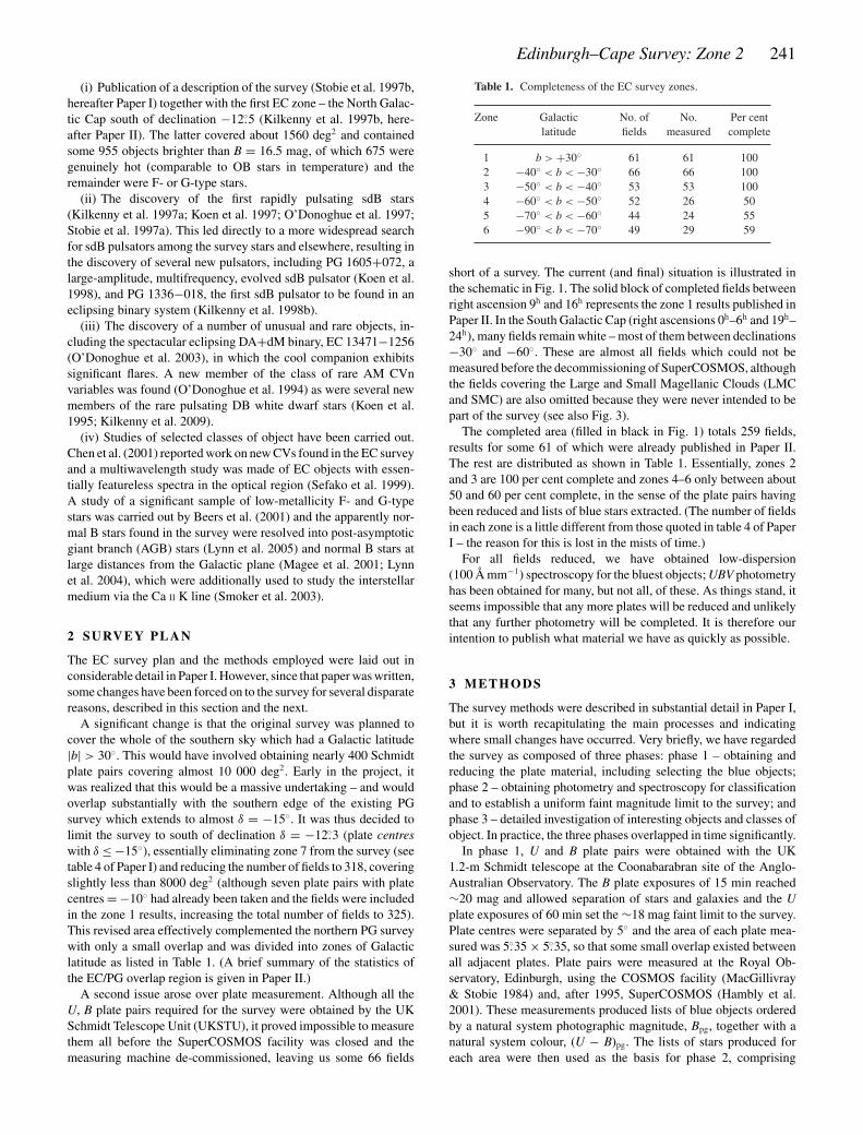
short of a survey. The current (and final) situation is illustrated inthe schematic in Fig. 1. The solid block of completed fields betweenright ascension 9h and 16h represents the zone 1 results published inPaper II. In the South Galactic Cap (right ascensions 0h–6h and 19h–24h), many fields remain white – most of them between declinations−30◦ and −60◦. These are almost all fields which could not bemeasured before the decommissioning of SuperCOSMOS, althoughthe fields covering the Large and Small Magellanic Clouds (LMCand SMC) are also omitted because they were never intended to bepart of the survey (see also Fig. 3).

The completed area (filled in black in Fig. 1) totals 259 fields,results for some 61 of which were already published in Paper II.The rest are distributed as shown in Table 1. Essentially, zones 2and 3 are 100 per cent complete and zones 4–6 only between about50 and 60 per cent complete, in the sense of the plate pairs havingbeen reduced and lists of blue stars extracted. (The number of fieldsin each zone is a little different from those quoted in table 4 of PaperI – the reason for this is lost in the mists of time.)

For all fields reduced, we have obtained low-dispersion(100 Å mm−1) spectroscopy for the bluest objects; UBV photometryhas been obtained for many, but not all, of these. As things stand, itseems impossible that any more plates will be reduced and unlikelythat any further photometry will be completed. It is therefore ourintention to publish what material we have as quickly as possible.

3 M E T H O D S

The survey methods were described in substantial detail in Paper I,but it is worth recapitulating the main processes and indicatingwhere small changes have occurred. Very briefly, we have regardedthe survey as composed of three phases: phase 1 – obtaining andreducing the plate material, including selecting the blue objects;phase 2 – obtaining photometry and spectroscopy for classificationand to establish a uniform faint magnitude limit to the survey; andphase 3 – detailed investigation of interesting objects and classes ofobject. In practice, the three phases overlapped in time significantly.

In phase 1, U and B plate pairs were obtained with the UK1.2-m Schmidt telescope at the Coonabarabran site of the Anglo-Australian Observatory. The B plate exposures of 15 min reached∼20 mag and allowed separation of stars and galaxies and the Uplate exposures of 60 min set the ∼18 mag faint limit to the survey.Plate centres were separated by 5◦ and the area of each plate mea-sured was 5.◦35 × 5.◦35, so that some small overlap existed betweenall adjacent plates. Plate pairs were measured at the Royal Ob-servatory, Edinburgh, using the COSMOS facility (MacGillivray& Stobie 1984) and, after 1995, SuperCOSMOS (Hambly et al.2001). These measurements produced lists of blue objects orderedby a natural system photographic magnitude, Bpg, together with anatural system colour, (U − B)pg. The lists of stars produced foreach area were then used as the basis for phase 2, comprising

242 D. O’Donoghue et al.

Figure 1. The EC survey: UKSTU fields actually scanned and reduced are black. Because this is only a schematic, the apparently large field at the southcelestial pole (bottom of the figure) has the same area as the apparently tiny equatorial fields at the top. Some fields with δ >−15◦ were obtained before thedecision was taken not to do the equatorial zone (zone 7). The holes at bottom right around fields 56 and 29 are the LMC and SMC areas, respectively, whichwere purposely excluded from the survey. Zone 1 is the solid area at top, centre and zone 7 would have extended the Galactic Caps to the equator. The SouthGalactic Pole is in UKSTU area 411.

a single photoelectric UBV measurement and low-dispersion(100 Å mm−1) spectrogram for each blue object down to a con-sistent limiting magnitude of B = 16.5, carried out at the SouthAfrican Astronomical Observatory (SAAO). Results from someof the phase 3 programmes have already been briefly noted inSection 1.

A change in the method of blue object selection (from the reducedphotographic material) was made with the switch from COSMOSto SuperCOSMOS. The original selection was made in the photo-graphic natural system using a B/(U − B) colour–magnitude plot(see fig. 2 of Paper I). A polygon, fitted by eye, was used to separatethe relatively small number of very blue objects from the vast num-bers of redder ones. In the more recently reduced fields, a processwas used of selecting objects starting with the bluest and proceedingredwards until a sharp increase in numbers was detected – effec-tively the onset of systematic detection of F- and G-type field stars.At the phase 2 stage – obtaining photometry and spectroscopy of theblue objects – we started observing each area at the brightest objectsand progressed until the first object with B fainter than 16.5 mag wasreached. Simultaneously, we observed the (photographically) bluestobjects first and progressed towards redder objects until we began

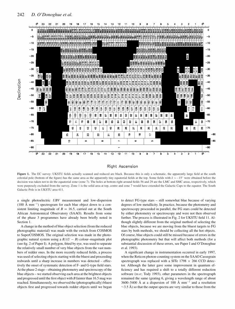
to detect FG-type stars – still somewhat blue because of varyingdegrees of low metallicity. In practice, because the photometry andspectroscopy proceeded in parallel, the FG stars could be detectedby either photometry or spectroscopy and were not then observedfurther. The process is illustrated in Fig. 2 for UKSTU field 11. Al-though slightly different from the original method of selecting theblue objects, because we are moving from the bluest targets to FGstars by both methods, we should be collecting all the hot objects.Of course, blue objects could still be missed because of errors in thephotographic photometry but that will affect both methods (for asubstantial discussion of these errors, see Paper I and O’Donoghueet al. 1993).

A significant change in instrumentation occurred in early 1997,when the Reticon photon-counting system on the SAAO Cassegrainspectrograph was replaced with a SITe 1798 × 266 CCD detec-tor. Although the latter gave some improvement in quantum ef-ficiency and has required a shift to a totally different reductionsoftware (IRAF; Tody 1993), other parameters in the spectrographremained the same (grating 6, giving a wavelength range of about3600–5400 Å at a dispersion of 100 Å mm−1 and a resolution∼3.5 Å) so that the output spectra are very similar to those from the

Edinburgh–Cape Survey: Zone 2 243

Figure 2. Blue object observations in UKSTU field 11 (as an example).The natural system photographic B/(U − B) colour–magnitude diagram isplotted. Starting from the brightest objects and working towards fainter andredder objects, the red limit is set by the detection of FG stars (•) and thefaint limit is set by the detection of the first star with a photoelectric Bmagnitude fainter than 16.5 mag. In this particular field, hot subdwarfs (�),white dwarfs (�) and AGN (©) are found down to the B = 16.5 limit. Theother objects (+) remain unclassified but, brighter than B = 16.5, are mostprobably F- and G-type stars.

Reticon and the spectral classification process should be essentiallyunaffected.

4 ZO N E 2

As noted in Section 2, the survey is limited to plate centres southof declination δ = −15◦ and thus to a northern declination limitof about δ = −12.◦3◦. Zone 2 is additionally defined by selectingUKSTU field centres with Galactic latitudes in the range −30◦

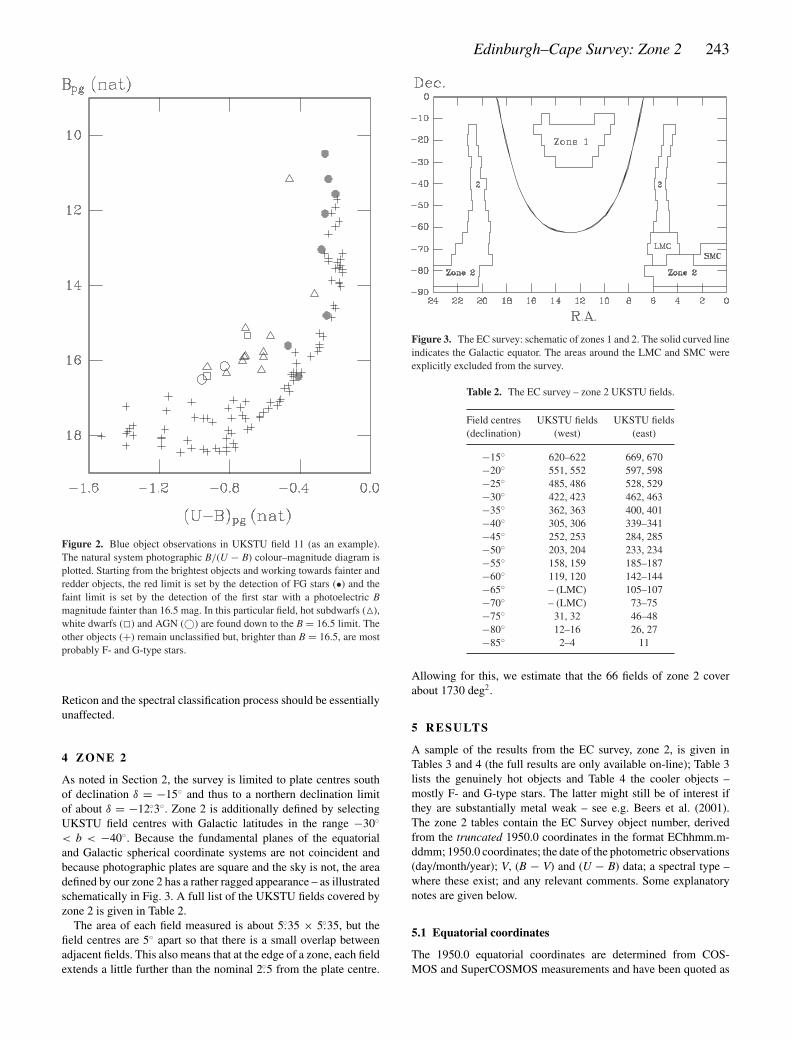
< b < −40◦. Because the fundamental planes of the equatorialand Galactic spherical coordinate systems are not coincident andbecause photographic plates are square and the sky is not, the areadefined by our zone 2 has a rather ragged appearance – as illustratedschematically in Fig. 3. A full list of the UKSTU fields covered byzone 2 is given in Table 2.

The area of each field measured is about 5.◦35 × 5.◦35, but thefield centres are 5◦ apart so that there is a small overlap betweenadjacent fields. This also means that at the edge of a zone, each fieldextends a little further than the nominal 2.◦5 from the plate centre.

Figure 3. The EC survey: schematic of zones 1 and 2. The solid curved lineindicates the Galactic equator. The areas around the LMC and SMC wereexplicitly excluded from the survey.

Table 2. The EC survey – zone 2 UKSTU fields.

Field centres UKSTU fields UKSTU fields(declination) (west) (east)

−15◦ 620–622 669, 670−20◦ 551, 552 597, 598−25◦ 485, 486 528, 529−30◦ 422, 423 462, 463−35◦ 362, 363 400, 401−40◦ 305, 306 339–341−45◦ 252, 253 284, 285−50◦ 203, 204 233, 234−55◦ 158, 159 185–187−60◦ 119, 120 142–144−65◦ – (LMC) 105–107−70◦ – (LMC) 73–75−75◦ 31, 32 46–48−80◦ 12–16 26, 27−85◦ 2–4 11

Allowing for this, we estimate that the 66 fields of zone 2 coverabout 1730 deg2.

5 R ESULTS

A sample of the results from the EC survey, zone 2, is given inTables 3 and 4 (the full results are only available on-line); Table 3lists the genuinely hot objects and Table 4 the cooler objects –mostly F- and G-type stars. The latter might still be of interest ifthey are substantially metal weak – see e.g. Beers et al. (2001).The zone 2 tables contain the EC Survey object number, derivedfrom the truncated 1950.0 coordinates in the format EChhmm.m-ddmm; 1950.0 coordinates; the date of the photometric observations(day/month/year); V, (B − V) and (U − B) data; a spectral type –where these exist; and any relevant comments. Some explanatorynotes are given below.

5.1 Equatorial coordinates

The 1950.0 equatorial coordinates are determined from COS-MOS and SuperCOSMOS measurements and have been quoted as

244 D. O’Donoghue et al.

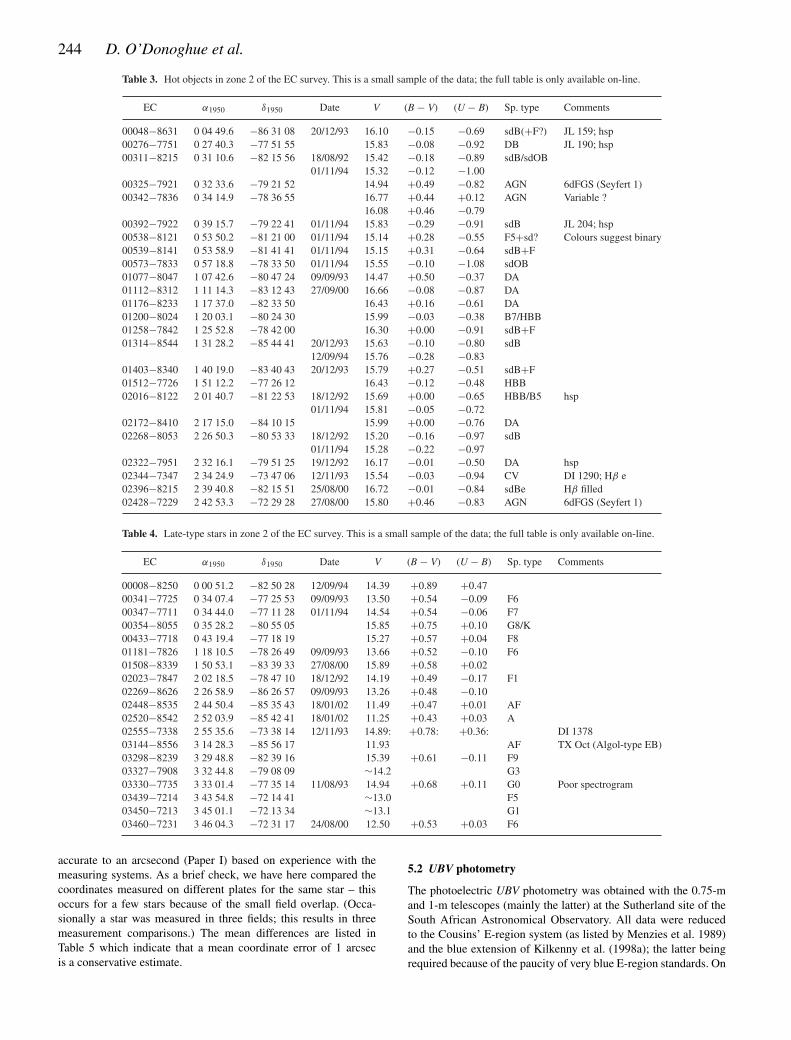
Table 3. Hot objects in zone 2 of the EC survey. This is a small sample of the data; the full table is only available on-line.

EC α1950 δ1950 Date V (B − V) (U − B) Sp. type Comments

00048−8631 0 04 49.6 −86 31 08 20/12/93 16.10 −0.15 −0.69 sdB(+F?) JL 159; hsp00276−7751 0 27 40.3 −77 51 55 15.83 −0.08 −0.92 DB JL 190; hsp00311−8215 0 31 10.6 −82 15 56 18/08/92 15.42 −0.18 −0.89 sdB/sdOB

01/11/94 15.32 −0.12 −1.0000325−7921 0 32 33.6 −79 21 52 14.94 +0.49 −0.82 AGN 6dFGS (Seyfert 1)00342−7836 0 34 14.9 −78 36 55 16.77 +0.44 +0.12 AGN Variable ?

16.08 +0.46 −0.7900392−7922 0 39 15.7 −79 22 41 01/11/94 15.83 −0.29 −0.91 sdB JL 204; hsp00538−8121 0 53 50.2 −81 21 00 01/11/94 15.14 +0.28 −0.55 F5+sd? Colours suggest binary00539−8141 0 53 58.9 −81 41 41 01/11/94 15.15 +0.31 −0.64 sdB+F00573−7833 0 57 18.8 −78 33 50 01/11/94 15.55 −0.10 −1.08 sdOB01077−8047 1 07 42.6 −80 47 24 09/09/93 14.47 +0.50 −0.37 DA01112−8312 1 11 14.3 −83 12 43 27/09/00 16.66 −0.08 −0.87 DA01176−8233 1 17 37.0 −82 33 50 16.43 +0.16 −0.61 DA01200−8024 1 20 03.1 −80 24 30 15.99 −0.03 −0.38 B7/HBB01258−7842 1 25 52.8 −78 42 00 16.30 +0.00 −0.91 sdB+F01314−8544 1 31 28.2 −85 44 41 20/12/93 15.63 −0.10 −0.80 sdB

12/09/94 15.76 −0.28 −0.8301403−8340 1 40 19.0 −83 40 43 20/12/93 15.79 +0.27 −0.51 sdB+F01512−7726 1 51 12.2 −77 26 12 16.43 −0.12 −0.48 HBB02016−8122 2 01 40.7 −81 22 53 18/12/92 15.69 +0.00 −0.65 HBB/B5 hsp

01/11/94 15.81 −0.05 −0.7202172−8410 2 17 15.0 −84 10 15 15.99 +0.00 −0.76 DA02268−8053 2 26 50.3 −80 53 33 18/12/92 15.20 −0.16 −0.97 sdB

01/11/94 15.28 −0.22 −0.9702322−7951 2 32 16.1 −79 51 25 19/12/92 16.17 −0.01 −0.50 DA hsp02344−7347 2 34 24.9 −73 47 06 12/11/93 15.54 −0.03 −0.94 CV DI 1290; Hβ e02396−8215 2 39 40.8 −82 15 51 25/08/00 16.72 −0.01 −0.84 sdBe Hβ filled02428−7229 2 42 53.3 −72 29 28 27/08/00 15.80 +0.46 −0.83 AGN 6dFGS (Seyfert 1)

Table 4. Late-type stars in zone 2 of the EC survey. This is a small sample of the data; the full table is only available on-line.

EC α1950 δ1950 Date V (B − V) (U − B) Sp. type Comments

00008−8250 0 00 51.2 −82 50 28 12/09/94 14.39 +0.89 +0.4700341−7725 0 34 07.4 −77 25 53 09/09/93 13.50 +0.54 −0.09 F600347−7711 0 34 44.0 −77 11 28 01/11/94 14.54 +0.54 −0.06 F700354−8055 0 35 28.2 −80 55 05 15.85 +0.75 +0.10 G8/K00433−7718 0 43 19.4 −77 18 19 15.27 +0.57 +0.04 F801181−7826 1 18 10.5 −78 26 49 09/09/93 13.66 +0.52 −0.10 F601508−8339 1 50 53.1 −83 39 33 27/08/00 15.89 +0.58 +0.0202023−7847 2 02 18.5 −78 47 10 18/12/92 14.19 +0.49 −0.17 F102269−8626 2 26 58.9 −86 26 57 09/09/93 13.26 +0.48 −0.1002448−8535 2 44 50.4 −85 35 43 18/01/02 11.49 +0.47 +0.01 AF02520−8542 2 52 03.9 −85 42 41 18/01/02 11.25 +0.43 +0.03 A02555−7338 2 55 35.6 −73 38 14 12/11/93 14.89: +0.78: +0.36: DI 137803144−8556 3 14 28.3 −85 56 17 11.93 AF TX Oct (Algol-type EB)03298−8239 3 29 48.8 −82 39 16 15.39 +0.61 −0.11 F903327−7908 3 32 44.8 −79 08 09 ∼14.2 G303330−7735 3 33 01.4 −77 35 14 11/08/93 14.94 +0.68 +0.11 G0 Poor spectrogram03439−7214 3 43 54.8 −72 14 41 ∼13.0 F503450−7213 3 45 01.1 −72 13 34 ∼13.1 G103460−7231 3 46 04.3 −72 31 17 24/08/00 12.50 +0.53 +0.03 F6

accurate to an arcsecond (Paper I) based on experience with themeasuring systems. As a brief check, we have here compared thecoordinates measured on different plates for the same star – thisoccurs for a few stars because of the small field overlap. (Occa-sionally a star was measured in three fields; this results in threemeasurement comparisons.) The mean differences are listed inTable 5 which indicate that a mean coordinate error of 1 arcsecis a conservative estimate.

5.2 UBV photometry

The photoelectric UBV photometry was obtained with the 0.75-mand 1-m telescopes (mainly the latter) at the Sutherland site of theSouth African Astronomical Observatory. All data were reducedto the Cousins’ E-region system (as listed by Menzies et al. 1989)and the blue extension of Kilkenny et al. (1998a); the latter beingrequired because of the paucity of very blue E-region standards. On

Edinburgh–Cape Survey: Zone 2 245

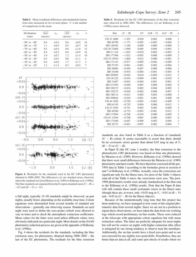
Table 5. Mean coordinate differences and standard deviationsfrom stars measured on two or more plates. ‘n’ is the numberof comparisons in the mean.

Declination |�α| σα |�δ| σ δ nzones (arcsec) (arcsec)

−90◦ to −80◦ 0.6 ±0.4 0.6 ±0.9 34−80◦ to −70◦ 1.1 ±0.8 0.5 ±0.7 19−70◦ to −60◦ 0.5 ±0.4 0.8 ±1.0 14−60◦ to −50◦ 0.4 ±0.5 0.6 ±0.9 16−50◦ to −40◦ 1.0 ±0.7 1.2 ±1.4 10−40◦ to −30◦ 0.3 ±0.5 0.8 ±1.1 4−30◦ to −20◦ 0.4 ±0.6 1.7 ±1.7 3−10◦ to −20◦ 1.2 ±1.4 0.3 ±0.5 7

Figure 4. Residuals for the standards used in the EC UBV photometryobtained in 2000–2002. The differences (�) are standard minus observed,where the standards are from Menzies et al. (1989) or Kilkenny et al. (1998a).The blue standards are separated from the E-region standards near (U − B) =−0.5 and (B − V) = −0.1.

a full night, typically 15–20 standards might be observed; on partnights, usually fewer, depending on the available clear time. Colourequations were determined from several months of standard starobservations – generally one observing season. Standards on eachnight were used to define the zero-points (which were allowed tovary in time) and to check the atmospheric extinction coefficients.Mean values for the latter were used unless different values wereobviously indicated on a particular night. More details on the SAAOphotometry reduction process are given in the appendix of Kilkennyet al. (1998a).

Fig. 4 shows the residuals for the standards, including the blueextension stars, for photometry obtained during 2000–2002 – thelast of the EC photometry. The residuals for the blue extension

Table 6. Residuals for the EC UBV photometry of the blue extensionstars observed in 2000–2001. The differences (�) are Kilkenny et al.(1998a) minus observed.

Star (U − B) �V �(B − V) �(U − B) n

CD-31 4800 −1.207 0.020 0.002 0.000 1HD 49798 −1.173 − 0.002 − 0.002 − 0.004 2

HD 149382 −1.108 0.009 0.000 − 0.008 3CD-28 7246S −1.098 0.005 0.004 − 0.001 1

BD-11 162 −1.043 − 0.010 0.002 − 0.002 4HD 177566 −1.012 − 0.003 0.000 − 0.009 2

CD-35 15910 −1.004 0.023 0.000 − 0.001 4HD 171141 −0.977 − 0.005 − 0.002 − 0.009 3

HD 57193 −0.961 − 0.001 0.002 − 0.004 1HD 56094 −0.956 0.007 0.000 0.000 1HD 18100 −0.954 − 0.004 − 0.001 − 0.003 8

HD 205805 −0.945 0.010 − 0.002 − 0.012 3CD-38 222 −0.934 − 0.009 0.001 − 0.010 4HD 31407 −0.862 − 0.004 0.001 0.001 5

HD 217505 −0.840 0.003 0.000 0.002 9HD 220172 −0.834 0.005 0.004 0.005 1HD 192273 −0.828 − 0.002 0.008 0.007 3HD 188112 −0.813 0.002 0.003 − 0.008 1HD 209684 −0.810 − 0.001 0.001 0.008 10

CD-44 1028 −0.799 − 0.002 − 0.003 − 0.009 3HD 61193 −0.755 0.004 0.000 0.012 1

CD-33 2585 −0.751 0.003 0.002 0.009 3HD 49260 −0.732 − 0.003 − 0.001 0.012 3

HD 173994 −0.708 − 0.010 0.000 0.005 2CD-41 14294 −0.700 0.001 0.000 0.003 6

HD 171940 −0.687 − 0.009 0.003 0.004 3HD 36733 −0.663 − 0.007 0.002 0.004 7

standards are also listed in Table 6 as a function of (standard)(U − B) colour. It seems reasonable to assert that there shouldbe no systematic errors greater than about 0.01 mag in any of V,(B − V) or (U − B).

In Paper II (the EC zone 1 results), the blue extension to thephotoelectric UBV photometry was based on blue star photometryby Menzies et al. (1989). However, Kilkenny et al. (1998a) showedthat there were small differences between the Menzies et al. (1989)photometry and later results. We have therefore corrected all the pre-1995 data in Table 3 according to the formulae given in sections 6and 7 of Kilkenny et al. (1998a). Actually, since the corrections aresignificant only for the bluest stars, for most of the Table 3 objects(and all of the Table 4 stars), the corrections were zero. The post-1998 photometric results were already standardized at the blue endto the Kilkenny et al. (1998a) results. Note that the Paper II datawill still contain these small systematic errors in the bluest stars(though these are, at worst, only +0.03 mag in V, −0.01 in (B − V)and −0.02 in (U − B) for the bluest objects).

Because of the unintentionally long time that this project hasbeen underway, we have managed to lose some of the original pho-tometric data from several nights. Since we are not in a position torepeat these observations, we have taken the data from our workinglogs which record preliminary on-line results. These were reducedat the telescope with appropriate colour equations but with meanextinction values. The latter are perfectly adequate for most nightsbut will not be correct on nights with higher extinction (this effectis mitigated by our strong tendency to observe near the meridian).Additionally, the on-line results have a fixed zero-point and so arenot corrected for any nightly zero-point drifts. Nonetheless, they arebetter than no data at all, and some spot checks of results where we

246 D. O’Donoghue et al.

have both preliminary and final data, indicate that the vast majorityof differences between these results are in the range 0.00–0.03 mag.However, occasionally larger residuals do occur, so that these pre-liminary data should be treated with appropriate caution. In thetables, such photometric data are indicated by the absence of a dateof observation.

Where we have no photometry at all (with one exception, thisapplies only to the Table 4 stars), we have used SIMBAD to searchfor published V magnitudes and have included these in the tables,often with an indication of the source in the ‘comments’ column.(Note, however, that this might not be the original source, given thatthe SIMBAD data base is a compilation). If there is no magnitudeto be found in the literature, we have estimated a magnitude fromthe photographic photometry. These estimates are indicated with atilde (∼) in the tables and should be regarded as very rough; partlydue to the inherent inaccuracy in photographic data and partly dueto the fact that we cannot generally apply colour equations to theseresults.

5.3 Spectral types

As far as possible, we have obtained low-dispersion (100 Å mm−1)spectrograms for all objects – with the particular exception of ob-jects which appear to be F-type or later from the UBV photometry.Spectrograms were obtained with grating 6 (coverage about 3600–5400 Å and resolution ∼3.5 Å) in the Unit Spectrograph on the1.9-m telescope at the Sutherland site of the SAAO. In the earlydays of the survey, the spectrograph was equipped with a Reticondetector but since about 1997 has used a CCD detector. Figs 9–14in Paper I give examples of some of the Reticon spectra. In a fewcases, particularly with poor signal-to-noise ratio (S/N) and/or spec-tra which appear to show no features in the grating 6 spectrograms,we have also obtained grating 7 data (210 Å mm−1, with a coverageof about 3600–7200 Å and resolution of ∼7 Å).

Paper I also describes the basis of our classification process –which we have tried to maintain in this paper. In brief, we haveused the scheme proposed by Moehler et al. (1990) for the hotsubdwarf stars. These are usually obvious by their relatively broad(high-gravity) spectral lines: sdB types show hydrogen and weak(or no) He I; sdOB stars have hydrogen and weak He I and He II;and sdO stars show hydrogen and He II. In addition, the helium-rich subdwarfs are typified by having no (or very weak) hydrogen:He-sdB stars are indicated by strong He I and perhaps weak He II;He-sdO types typically have strong He II and weak He I (if Balmerseries lines were present, they would be blended with He II features).A blue horizontal branch (HBB) type is indicated by moderatelystrong H lines and weak He I (4471) and perhaps Mg II (4481).We have often found it difficult to decide whether a star shouldbe classified as a normal B star or an HBB (and it is sometimeshard, when classifying, to fight off the prejudice that normal B starsshould be much less likely in high-latitude surveys). Poor S/N of thespectrograms compounds this problem – and sometimes results ina classification of the type Bn/HBB (or HBB/Bn), when we cannotdecide.

Our spectra extend to well below the Balmer discontinuity andthat has been a useful classification indicator. In the hot subdwarfs,the Balmer lines are typically seen only to about n = 10–12, whereasin normal B stars, they are often visible to n = 13–14 (depending,of course, on the S/N of the spectrograms). The HBB stars mighthave even more lines visible; the white dwarfs will have far fewervisible lines, typically only to n = 8.

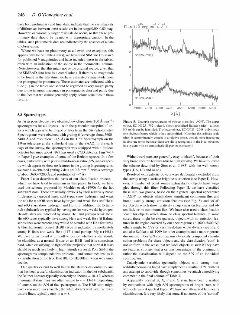
Figure 5. Example spectrograms of objects classified ‘AGN’. The upperobject, EC 00325−7921, clearly shows redshifted Balmer series – at leastHβ to Hε can be identified. The lower object, EC 05023−2948, only showsone obvious feature which is thus unidentified. [Note that the ordinate scale(flux) is approximately correct in a relative sense, though more inaccuratein absolute terms because these are slit spectrograms in the blue, obtainedin a system with no atmospheric dispersion corrector.]

White dwarf stars are generally easy to classify because of theirvery broad spectral features (due to high gravity). We have followedthe scheme described by Sion et al. (1983) with the well-knowntypes (DA, DB and so on).

Resolved extragalactic objects were deliberately excluded fromthe survey using a surface brightness criterion (see Paper I). How-ever, a number of point source extragalactic objects have wrig-gled through this filter. Following Paper II, we have classifiedthese into two groups, based on their general spectral appearance– ‘AGN’ for objects which show significant continuum flux andbroad, usually strong, emission features (see Fig. 5)–and ‘eGal’for objects which show relatively sharp emission features and of-ten little or no continuum flux. We have also used a classification‘cont’ for objects which show no clear spectral features. In somecases, these might be extragalactic objects with no emission fea-tures in the region covered by our spectrograms (∼3600–5400 Å);others might be CVs or very weak-line white dwarfs (see Fig. 6and also Sefako et al. 1999 for other examples and a more rigorousdiscussion). Poor S/N spectrograms obviously compound classifi-cation problems for these objects and the classification ‘cont’ isnot uniform in the sense that we label objects as such if they haveno features stronger that a certain percentage of the continuum;rather the classification will depend on the S/N of an individualspectrogram.

Cataclysmic variables (generally, objects with strong, non-redshifted emission lines) have simply been classified ‘CV’ withoutany attempt to subdivide, though sometimes we attach a modifyingcomment in the final column of Table 3.

Apparently normal B, A, F and G stars have been classifiedby comparison with high S/N spectrograms of bright stars withwell-determined spectral types. We have not attempted luminosityclassification. It is very likely that some, if not most, of the ‘normal’

Edinburgh–Cape Survey: Zone 2 247

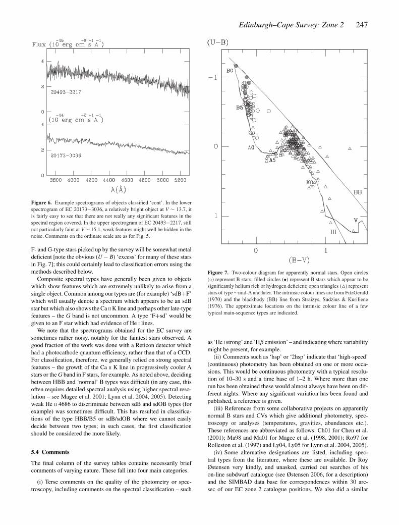
Figure 6. Example spectrograms of objects classified ‘cont’. In the lowerspectrogram of EC 20173−3036, a relatively bright object at V ∼ 13.7, itis fairly easy to see that there are not really any significant features in thespectral region covered. In the upper spectrogram of EC 20493−2217, stillnot particularly faint at V ∼ 15.1, weak features might well be hidden in thenoise. Comments on the ordinate scale are as for Fig. 5.

F- and G-type stars picked up by the survey will be somewhat metaldeficient [note the obvious (U − B) ‘excess’ for many of these starsin Fig. 7]; this could certainly lead to classification errors using themethods described below.

Composite spectral types have generally been given to objectswhich show features which are extremely unlikely to arise from asingle object. Common among our types are (for example) ‘sdB+F’which will usually denote a spectrum which appears to be an sdBstar but which also shows the Ca II K line and perhaps other late-typefeatures – the G band is not uncommon. A type ‘F+sd’ would begiven to an F star which had evidence of He I lines.

We note that the spectrograms obtained for the EC survey aresometimes rather noisy, notably for the faintest stars observed. Agood fraction of the work was done with a Reticon detector whichhad a photocathode quantum efficiency, rather than that of a CCD.For classification, therefore, we generally relied on strong spectralfeatures – the growth of the Ca II K line in progressively cooler Astars or the G band in F stars, for example. As noted above, decidingbetween HBB and ‘normal’ B types was difficult (in any case, thisoften requires detailed spectral analysis using higher spectral reso-lution – see Magee et al. 2001; Lynn et al. 2004, 2005). Detectingweak He II 4686 to discriminate between sdB and sdOB types (forexample) was sometimes difficult. This has resulted in classifica-tions of the type HBB/B5 or sdB/sdOB where we cannot easilydecide between two types; in such cases, the first classificationshould be considered the more likely.

5.4 Comments

The final column of the survey tables contains necessarily briefcomments of varying nature. These fall into four main categories.

(i) Terse comments on the quality of the photometry or spec-troscopy, including comments on the spectral classification – such

Figure 7. Two-colour diagram for apparently normal stars. Open circles(◦) represent B stars; filled circles (•) represent B stars which appear to besignificantly helium rich or hydrogen deficient; open triangles (�) representstars of type ∼mid-A and later. The intrinsic colour lines are from FitzGerald(1970) and the blackbody (BB) line from Straizys, Sudzius & Kuriliene(1976). The approximate locations on the intrinsic colour line of a fewtypical main-sequence types are indicated.

as ‘He I strong’ and ‘Hβ emission’ – and indicating where variabilitymight be present, for example.

(ii) Comments such as ‘hsp’ or ‘2hsp’ indicate that ‘high-speed’(continuous) photometry has been obtained on one or more occa-sions. This would be continuous photometry with a typical resolu-tion of 10–30 s and a time base of 1–2 h. Where more than onerun has been obtained these would almost always have been on dif-ferent nights. Where any significant variation has been found andpublished, a reference is given.

(iii) References from some collaborative projects on apparentlynormal B stars and CVs which give additional photometry, spec-troscopy or analyses (temperatures, gravities, abundances etc.).These references are abbreviated as follows: Ch01 for Chen et al.(2001); Ma98 and Ma01 for Magee et al. (1998, 2001); Ro97 forRolleston et al. (1997) and Ly04, Ly05 for Lynn et al. 2004, 2005).

(iv) Some alternative designations are listed, including spec-tral types from the literature, where these are available. Dr RoyØstensen very kindly, and unasked, carried out searches of hison-line subdwarf catalogue (see Østensen 2006, for a description)and the SIMBAD data base for correspondences within 30 arc-sec of our EC zone 2 catalogue positions. We also did a similar

248 D. O’Donoghue et al.

SIMBAD search within 15 arcsec of the EC positions, obtainingsimilar results.

With regard to the last category, an important caveat to keep inmind is that these alternative designations are in no way completeor exhaustive. Some stars, particularly the brighter ones, can havemany names, having been detected in different ground-based sur-veys (going back as far as the Durchmusterungen of the late 19thcentury) as well as in modern satellite surveys. The available spacepermits only one or two alternatives – and, in any case, the SIM-BAD data base is so widely used and so catholic in scope that thisis hardly a serious deficiency.

Our particular choices for alternatives might seem eclectic, evenwhimsical, but were decided on the basis of two main considera-tions: first, to select sources which contained additional informationsuch as spectral types. These include the BPS CS stars (Beers, Pre-ston & Schectman 1985), the 6-degree Field Galaxy Survey (6dFGS;Jones et al. 2004), the Hamburg–ESO survey (HE; Wisotzki et al.1996, for example), the white dwarf catalogues (WD; McCook &Sion 1999 – later versions are available on-line) and the cataloguesof quasars and AGN (VV; Veron-Cetty & Veron 2010, for example).We note that some of these references are compilations and oftennot the source of the spectral types – the HD stars in our table, forexample, have MK types from the extensive work of the Michigangroup (Houk 1978; Houk & Cowley 1975 etc.). Our second consid-eration was to select alternative designations from surveys whichoverlapped significantly with ours and were the original discoverysources. These include the JL stars (Jaidee & Lynga 1969) and theDI objects found in the Magellanic Cloud bridge (Demers & Irwin1991).

We have not generally referred to satellite data bases in the tables;there are quite a few EC objects which have been observed by Inter-national Ultraviolet Explorer (IUE), Extreme Ultraviolet Explorer(EUVE), Galaxy Evolution Explorer (GALEX) and so on, as wellas many included in the ground-based Two Micron All Sky Survey(2MASS) survey, but it would be impossible to include all these ina systematic and consistent way. As it is generally the actual mea-surements which are important, the reader is referred to SIMBADfor these data.

Finally, we note that the correlations we have made with othersources (using SIMBAD) are generally in good positional agree-ment. From 256 identifications, we find that 42 per cent agree tobetter than 1 arcsec (the accuracy claimed for our coordinates; seeTable 5) and 73 per cent to better than 2 arcsec. A few are as badas 5 or 6 arcsec and any correspondence worse than that has beenexcluded from the comments column (although significant propermotion could be an issue for the nearest objects, such as white dwarfstars). A small number of EC objects are close to ROSAT objects(1RSX; Voges et al. 1999) but, in general, the separations are of theorder 10 arcsec or more and we have not included these, although itcould be that for an extended object the X-rays come from a differ-ent region than the optical radiation. Again, the scrupulous readershould check SIMBAD for such coincidences.

6 TWO - C O L O U R D I AG R A M S

In a similar fashion to the zone 1 results (our Paper II), we presenttwo-colour diagrams for the principal classes of objects found inzone 2. Since most of the photometry presented here is only a singleobservation per target, estimating the errors is not easy. In Paper I,from a small number of objects with more than one observation,typical errors were estimated to vary from about 1 per cent for the

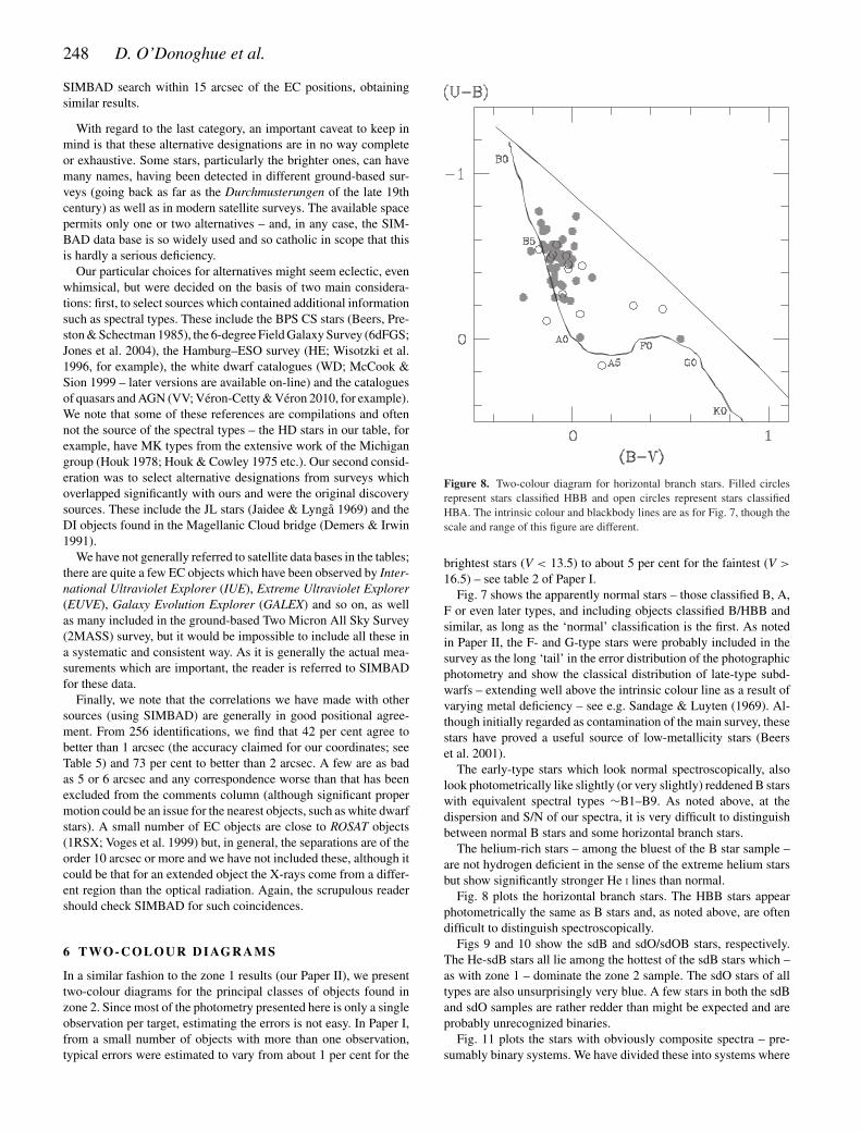
Figure 8. Two-colour diagram for horizontal branch stars. Filled circlesrepresent stars classified HBB and open circles represent stars classifiedHBA. The intrinsic colour and blackbody lines are as for Fig. 7, though thescale and range of this figure are different.

brightest stars (V < 13.5) to about 5 per cent for the faintest (V >

16.5) – see table 2 of Paper I.Fig. 7 shows the apparently normal stars – those classified B, A,

F or even later types, and including objects classified B/HBB andsimilar, as long as the ‘normal’ classification is the first. As notedin Paper II, the F- and G-type stars were probably included in thesurvey as the long ‘tail’ in the error distribution of the photographicphotometry and show the classical distribution of late-type subd-warfs – extending well above the intrinsic colour line as a result ofvarying metal deficiency – see e.g. Sandage & Luyten (1969). Al-though initially regarded as contamination of the main survey, thesestars have proved a useful source of low-metallicity stars (Beerset al. 2001).

The early-type stars which look normal spectroscopically, alsolook photometrically like slightly (or very slightly) reddened B starswith equivalent spectral types ∼B1–B9. As noted above, at thedispersion and S/N of our spectra, it is very difficult to distinguishbetween normal B stars and some horizontal branch stars.

The helium-rich stars – among the bluest of the B star sample –are not hydrogen deficient in the sense of the extreme helium starsbut show significantly stronger He I lines than normal.

Fig. 8 plots the horizontal branch stars. The HBB stars appearphotometrically the same as B stars and, as noted above, are oftendifficult to distinguish spectroscopically.

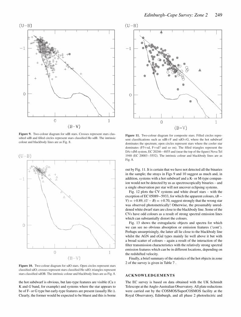
Figs 9 and 10 show the sdB and sdO/sdOB stars, respectively.The He-sdB stars all lie among the hottest of the sdB stars which –as with zone 1 – dominate the zone 2 sample. The sdO stars of alltypes are also unsurprisingly very blue. A few stars in both the sdBand sdO samples are rather redder than might be expected and areprobably unrecognized binaries.

Fig. 11 plots the stars with obviously composite spectra – pre-sumably binary systems. We have divided these into systems where

Edinburgh–Cape Survey: Zone 2 249

Figure 9. Two-colour diagram for sdB stars. Crosses represent stars clas-sified sdB and filled circles represent stars classified He-sdB. The intrinsiccolour and blackbody lines are as Fig. 8.

Figure 10. Two-colour diagram for sdO stars. Open circles represent starsclassified sdO; crosses represent stars classified He-sdO; triangles representstars classified sdOB. The intrinsic colour and blackbody lines are as Fig. 8.

the hot subdwarf is obvious, but late-type features are visible (Ca II

K and G band, for example) and systems where the star appears tobe of F- or G type but early-type features are present (usually He I).Clearly, the former would be expected to be bluest and this is borne

Figure 11. Two-colour diagram for composite stars. Filled circles repre-sent classifications such as sdB+F and sdO+G, where the hot subdwarfdominates the spectrum; open circles represent stars where the cooler stardominates (F5+sd, F+sd? and so on). The filled triangles represent theDA+dM system, EC 20246−4855 and (near the top of the figure) Nova Tel1948 (EC 20003−5552). The intrinsic colour and blackbody lines are asFig. 8.

out by Fig. 11. It is certain that we have not detected all the binariesin the sample; the strays in Figs 9 and 10 suggest as much and, inaddition, systems with a hot subdwarf and a K- or M-type compan-ion would not be detected by us as spectroscopically binaries – anda single observation per star will not uncover eclipsing systems.

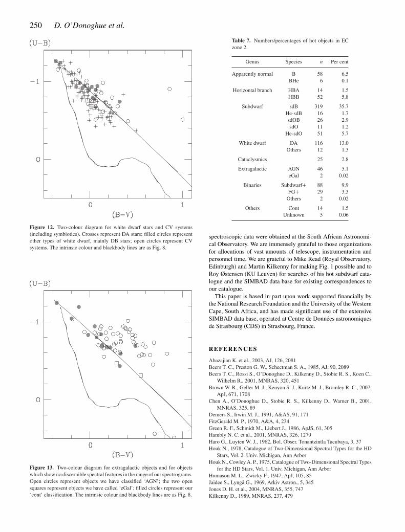
Fig. 12 plots the CV systems and white dwarf stars – with theexception of EC 05089−5933, for which the apparent colours, (B −V) = +0.89, (U − B) = +0.70, suggest strongly that the wrong starwas observed photometrically! Otherwise, the presumably unred-dened white dwarf stars are close to the blackbody line. Some of theCVs have odd colours as a result of strong spectral emission lineswhich can substantially distort the colours.

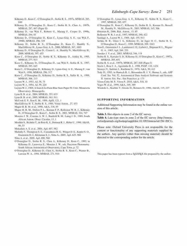
Fig. 13 shows the extragalactic objects and spectra for whichwe can see no obvious absorption or emission features (‘cont’).Perhaps unsurprisingly, the latter all lie close to the blackbody linewhilst the AGN and eGal types mainly lie well above it but witha broad scatter of colours – again a result of the interaction of thefilter transmission characteristics with the relatively strong spectralemission features which can be in different locations, depending onthe redshifted velocity.

Finally, a brief summary of the statistics of the hot objects in zone2 of the survey is given in Table 7 .

AC K N OW L E D G E M E N T S

The EC survey is based on data obtained with the UK SchmidtTelescope at the Anglo-Australian Observatory. All plate reductionswere carried out by the COSMOS/SuperCOSMOS facility at theRoyal Observatory, Edinburgh, and all phase 2 photoelectric and

250 D. O’Donoghue et al.

Figure 12. Two-colour diagram for white dwarf stars and CV systems(including symbiotics). Crosses represent DA stars; filled circles representother types of white dwarf, mainly DB stars; open circles represent CVsystems. The intrinsic colour and blackbody lines are as Fig. 8.

Figure 13. Two-colour diagram for extragalactic objects and for objectswhich show no discernible spectral features in the range of our spectrograms.Open circles represent objects we have classified ‘AGN’; the two opensquares represent objects we have called ‘eGal’; filled circles represent our‘cont’ classification. The intrinsic colour and blackbody lines are as Fig. 8.

Table 7. Numbers/percentages of hot objects in ECzone 2.

Genus Species n Per cent

Apparently normal B 58 6.5BHe 6 0.1

Horizontal branch HBA 14 1.5HBB 52 5.8

Subdwarf sdB 319 35.7He-sdB 16 1.7sdOB 26 2.9sdO 11 1.2

He-sdO 51 5.7

White dwarf DA 116 13.0Others 12 1.3

Cataclysmics 25 2.8

Extragalactic AGN 46 5.1eGal 2 0.02

Binaries Subdwarf+ 88 9.9FG+ 29 3.3

Others 2 0.02

Others Cont 14 1.5Unknown 5 0.06

spectroscopic data were obtained at the South African Astronomi-cal Observatory. We are immensely grateful to those organizationsfor allocations of vast amounts of telescope, instrumentation andpersonnel time. We are grateful to Mike Read (Royal Observatory,Edinburgh) and Martin Kilkenny for making Fig. 1 possible and toRoy Østensen (KU Leuven) for searches of his hot subdwarf cata-logue and the SIMBAD data base for existing correspondences toour catalogue.

This paper is based in part upon work supported financially bythe National Research Foundation and the University of the WesternCape, South Africa, and has made significant use of the extensiveSIMBAD data base, operated at Centre de Donnees astronomiquesde Strasbourg (CDS) in Strasbourg, France.

R E F E R E N C E S

Abazajian K. et al., 2003, AJ, 126, 2081Beers T. C., Preston G. W., Schectman S. A., 1985, AJ, 90, 2089Beers T. C., Rossi S., O’Donoghue D., Kilkenny D., Stobie R. S., Koen C.,

Wilhelm R., 2001, MNRAS, 320, 451Brown W. R., Geller M. J., Kenyon S. J., Kurtz M. J., Bromley R. C., 2007,

ApJ, 671, 1708Chen A., O’Donoghue D., Stobie R. S., Kilkenny D., Warner B., 2001,

MNRAS, 325, 89Demers S., Irwin M. J., 1991, A&AS, 91, 171FitzGerald M. P., 1970, A&A, 4, 234Green R. F., Schmidt M., Liebert J., 1986, ApJS, 61, 305Hambly N. C. et al., 2001, MNRAS, 326, 1279Haro G., Luyten W. J., 1962, Bol. Obser. Tonantzintla Tacubaya, 3, 37Houk N., 1978, Catalogue of Two-Dimensional Spectral Types for the HD

Stars, Vol. 2. Univ. Michigan, Ann ArborHouk N., Cowley A. P., 1975, Catalogue of Two-Dimensional Spectral Types

for the HD Stars, Vol. 1. Univ. Michigan, Ann ArborHumason M. L., Zwicky F., 1947, ApJ, 105, 85Jaidee S., Lynga G., 1969, Arkiv Astron., 5, 345Jones D. H. et al., 2004, MNRAS, 355, 747Kilkenny D., 1989, MNRAS, 237, 479

Edinburgh–Cape Survey: Zone 2 251

Kilkenny D., Koen C., O’Donoghue D., Stobie R. S., 1997a, MNRAS, 285,640

Kilkenny D., O’Donoghue D., Koen C., Stobie R. S., Chen A., 1997b,MNRAS, 287, 867 (Paper II)

Kilkenny D., van Wyk F., Roberts G., Marang F., Cooper D., 1998a,MNRAS, 294, 93

Kilkenny D., O’Donoghue D., Koen C., Lynas-Gray A. E., van Wyk F.,1998b, MNRAS, 296, 329

Kilkenny D., Stobie R. S., O’Donoghue D., Koen C., Hambly N.,MacGillivray H., Lynas-Gray A. E., 2006, MNRAS, 367, 1603

Kilkenny D., O’Donoghue D., Crause L. A., Hambly N., MacGillivray H.,2009, MNRAS, 397, 453

Koen C., O’Donoghue D., Stobie R. S., Kilkenny D., Ashley R., 1995,MNRAS, 277, 913

Koen C., Kilkenny D., O’Donoghue D., van Wyk F., Stobie R. S., 1997,MNRAS, 285, 645

Koen C., O’Donoghue D., Kilkenny D., Lynas-Gray A. E., Marang F., vanWyk F., 1998, MNRAS, 296, 317

Koen C., O’Donoghue D., Kilkenny D., Stobie R. S., Saffer R. A., 1999,MNRAS, 306, 213

Luyten W. J., 1953, AJ, 58, 75Luyten W. J., 1954, AJ, 59, 224Luyten W. J., 1969, A Search for Faint Blue Stars Paper 50. Univ. Minnesota

Observatory, MinneapolisLynn B. B. et al., 2004, MNRAS, 353, 633Lynn B. B. et al., 2005, MNRAS, 363, 911McCook G. P., Sion E. M., 1999, ApJS, 121, 1MacGillivray H. T., Stobie R. S., 1984, Vistas Astron., 27, 433Magee H. R. M. et al., 1998, A&A, 338, 85Magee H. R. M., Dufton P. L., Keenan F. P., Rolleston W. R. J., Kilkenny

D., O’Donoghue D., Koen C., Stobie R. S., 2001, MNRAS, 324, 747Menzies J. W., Cousins A. W. J., Banfield R. M., Laing J. D., 1989, South

African Astron. Obser. Circular, 13, 1Moehler S., Richtler T., de Boer K. S., Dettmar R. J., Heber U., 1990, A&AS,

86, 53Mukadam A. S. et al., 2004, ApJ, 607, 982Mullally F., Thompson S. E., Castanheira B. G., Winget D. E., Kepler S. O.,

Eisenstein D. J., Kleinman S. J., Nitta A., 2005, ApJ, 625, 966Nitta A. et al., 2009, ApJ, 690, 560O’Donoghue D., Stobie R. S., Chen A., Kilkenny D., Koen C., 1993, in

Kilkenny D., Lastovica E., Menzies J. W., eds, Precision Photometry.South African Astronomical Observatory, Cape Town, p. 72

O’Donoghue D., Kilkenny D., Chen A., Stobie R. S., Koen C., Warner B.,Lawson W. A., 1994, MNRAS, 271, 910

O’Donoghue D., Lynas-Gray A. E., Kilkenny D., Stobie R. S., Koen C.,1997, MNRAS, 285, 657

O’Donoghue D., Koen C., Kilkenny D., Stobie R. S., Koester D., BessellM., Hambly N., McGillivray H., 2003, MNRAS, 345, 506

Østensen R., 2006, Balt. Astron., 15, 85Rolleston W. R. J. et al., 1997, MNRAS, 290, 422Sandage A., Luyten W. J., 1969, ApJ, 155, 913Sefako R. R., Glass I. S., Kilkenny D., de Jager O. C., Stobie R. S.,

O’Donoghue D., Koen C., 1999, MNRAS, 309, 1043Sion E., Greenstein J. L., Landstreet J. D., Liebert J., Shipman H. L., Wegner

G. A., 1983, ApJ, 269, 253Smoker J. V. et al., 2003, MNRAS, 346, 119Stobie R. S., Kawaler S. D., Kilkenny D., O’Donoghue D., Koen C., 1997a,

MNRAS, 285, 651Stobie R. S. et al., 1997b, MNRAS, 287, 848 (Paper I)Stock J., Rose J. A., Agostinho R. J., 1998, PASP, 110, 1434Straizys V., Sudzius J., Kuriliene G., 1976, A&A, 50, 413Tody D., 1993, in Hanisch R. J., Brissenden R. J. V., Barnes J., eds, ASP

Conf. Ser. Vol. 52, Astronomical Data Analysis Software and SystemsII. Astron. Soc. Pac., San Francisco, p. 173

Veron-Cetty M. P., Veron P., 2010, A&A, 518, 10Voges W. et al., 1999, A&A, 349, 389Wisotzki L., Koehler T., Groote D., Reimers D., 1996, A&AS, 115, 227

S U P P O RT I N G IN F O R M AT I O N

Additional Supporting Information may be found in the online ver-sion of this article:

Table 3. Hot objects in zone 2 of the EC survey.Table 4. Late-type stars in zone 2 of the EC survey (http://mnras.oxfordjournals.org/lookup/suppl/doi:10.1093/mnras/stt158/-/DC1).

Please note: Oxford University Press is not responsible for thecontent or functionality of any supporting materials supplied bythe authors. Any queries (other than missing material) should bedirected to the corresponding author for the article.

This paper has been typeset from a TEX/LATEX file prepared by the author.