Iowa State UniversityDigital Repository @ Iowa State University

Graduate Theses and Dissertations Graduate College

2012

The edit distance function for graphs: anexploration of the case of forbidden induced K2,tand other questionsTracy Jean McKayIowa State University

Follow this and additional works at: http://lib.dr.iastate.edu/etdPart of the Mathematics Commons

This Dissertation is brought to you for free and open access by the Graduate College at Digital Repository @ Iowa State University. It has been acceptedfor inclusion in Graduate Theses and Dissertations by an authorized administrator of Digital Repository @ Iowa State University. For moreinformation, please contact hinefuku@iastate.edu.

Recommended CitationMcKay, Tracy Jean, "The edit distance function for graphs: an exploration of the case of forbidden induced K2,t and other questions"(2012). Graduate Theses and Dissertations. Paper 12401.

The edit distance function for graphs: an exploration of the case of forbidden

induced K2,t and other questions

by

Tracy J. McKay

A dissertation submitted to the graduate faculty

in partial fulfillment of the requirements for the degree of

DOCTOR OF PHILOSOPHY

Major: Mathematics

Program of Study Committee:

Ryan Martin, Major Professor

Maria Axenovich

Oliver Eulenstein

Leslie Hogben

Sung Song

Iowa State University

Ames, Iowa

2012

ii

DEDICATION

To my grandfather (Richards).

iii

TABLE OF CONTENTS

ACKNOWLEDGEMENTS . . . . . . . . . . . . . . . . . . . . . . . . . . . . . . . v

ABSTRACT . . . . . . . . . . . . . . . . . . . . . . . . . . . . . . . . . . . . . . . . vi

CHAPTER 1. INTRODUCTION . . . . . . . . . . . . . . . . . . . . . . . . . . 1

1.1 Definitions . . . . . . . . . . . . . . . . . . . . . . . . . . . . . . . . . . . . . . . 2

1.1.1 Simple graph terminology and notation . . . . . . . . . . . . . . . . . . 2

1.1.2 Terminology and notation specific to the problem . . . . . . . . . . . . . 4

1.2 Select review of the literature and past results . . . . . . . . . . . . . . . . . . . 7

1.3 Results . . . . . . . . . . . . . . . . . . . . . . . . . . . . . . . . . . . . . . . . . 13

CHAPTER 2. PROOFS FOR RESULTS FROM [34] . . . . . . . . . . . . . . 16

2.1 Preliminary results and observations . . . . . . . . . . . . . . . . . . . . . . . . 16

2.2 Proof of Theorem 18 . . . . . . . . . . . . . . . . . . . . . . . . . . . . . . . . . 19

2.3 Proof of Theorem 19 . . . . . . . . . . . . . . . . . . . . . . . . . . . . . . . . . 22

2.3.1 Upper bounds . . . . . . . . . . . . . . . . . . . . . . . . . . . . . . . . . 22

2.3.2 Lower bounds . . . . . . . . . . . . . . . . . . . . . . . . . . . . . . . . . 23

2.4 Proofs of Theorems 20, 21 and 22 . . . . . . . . . . . . . . . . . . . . . . . . . . 32

2.4.1 An extension of the known interval for K2,t . . . . . . . . . . . . . . . . 32

2.4.2 A construction for odd t . . . . . . . . . . . . . . . . . . . . . . . . . . . 33

2.4.3 A general lower bound for t . . . . . . . . . . . . . . . . . . . . . . . . . 34

2.5 Upper bound constructions . . . . . . . . . . . . . . . . . . . . . . . . . . . . . 36

2.5.1 Results from strongly regular graph constructions . . . . . . . . . . . . 36

2.5.2 Cycle construction . . . . . . . . . . . . . . . . . . . . . . . . . . . . . . 37

2.5.3 Furedi constructions . . . . . . . . . . . . . . . . . . . . . . . . . . . . . 38

iv

2.6 Figures . . . . . . . . . . . . . . . . . . . . . . . . . . . . . . . . . . . . . . . . 42

CHAPTER 3. MORE ON CYCLE POWERS AND FUREDI’S CONSTRUC-

TION . . . . . . . . . . . . . . . . . . . . . . . . . . . . . . . . . . . . . . . . . . 47

3.1 General cycle constructions . . . . . . . . . . . . . . . . . . . . . . . . . . . . . 47

3.1.1 The best k for a given value of r . . . . . . . . . . . . . . . . . . . . . . 47

3.1.2 Why r = 2 is optimal . . . . . . . . . . . . . . . . . . . . . . . . . . . . 48

3.2 Furedi’s construction from [29] described . . . . . . . . . . . . . . . . . . . . . . 49

CHAPTER 4. CONCLUSIONS AND FUTURE DIRECTIONS . . . . . . . . 50

BIBLIOGRAPHY . . . . . . . . . . . . . . . . . . . . . . . . . . . . . . . . . . . . 52

v

ACKNOWLEDGEMENTS

First and foremost, I would like to thank my adviser Ryan Martin for all of his guidance,

insight, and encouragement throughout the process of completing this thesis. I would also like

to thank all of the members of my POS Committee for their help, support, and valuable advice.

In particular, I would like to thank Prof. Hogben for her feedback on the manuscript of this

thesis, Prof. Song for important discussions about strongly regular graphs (including directing

me to Andries Brouwer’s website), and Maria Axenovich for pointing me in the direction of

Zolan Furedi’s K2,t-free constructions. Ed Marchant, Andrew Thomason, and Stephen Hartke

also contributed helpful conversations and information to my adviser, which he, in turn, passed

along to me.

In addition, I would like to thank the Mathematics Department at Iowa State for giving

me the chance to participate in so many enriching opportunities during my time here, and for

both travel support and a semester of research on the Wolfe Research Fellowship.

Last, but certainly not least, I would like to thank all of the office staff for everything that

they have done for me along the way.

vi

ABSTRACT

This thesis examines the edit distance function for principal hereditary properties of the

form Forb(K2,t), the hereditary property of graphs containing no induced bipartite subgraph on

2 and t vertices. It explores applications of several methods from the literature for determining

these edit distance functions, and also constructions from classical graph theory problems that

can be used to create colored regularity graphs leading to upper bounds on the functions.

Results include the entire edit distance function when t = 3 and 4, as well as bounds for

larger values of t, including the result that the maximum value of the function occurs over a

nondegenerate interval of values for odd t.

1

CHAPTER 1. INTRODUCTION

This thesis explores results for the edit distance function for graph properties of the form

Forb(K2,t). A simple graph G is described by a 2-tuple (V (G), E(G)), where V (G) is the set

of vertices of G, and E(G) ⊆ V (G)(2) is the set of edges of G (V (G)(2) denotes the subsets

of V (G) with order 2). Given two simple graphs G and G′ on the same vertex set V , the

edit distance between G and G′, denoted dist(G,G′), is the order of the symmetric difference

between E(G) and E(G′). Perhaps a more intuitive way to calculate edit distance is to ask

the question “How many edges would I need to add or delete in G to turn it into G′?” Edit

distance can be extended to measure the distance from a single graph G to an entire set of

graphs, or graph property, in a similar way. The edit distance function for a specific graph

property explores the asymptotic (in terms of the order of V (G)) behavior of the maximum

edit distance of any graph G with edge-density p from the property.

Problems involving adding and/or deleting edges from graphs are called edge-modification

problems. Edge-modification problems have a number of potential applications to chemistry,

biology, and the social sciences. These problems were one motivation for the initial exploration

of the edit distance function (see [5] and [7]). However, determining the edit distance function

for any single property can pose unique challenges, which rely on connections to classical graph

theory problems, that are interesting in their own right.

This thesis will explore some of the work that has already been done regarding edit distance

and the edit distance function, and then describe techniques and constructions used to generate

the new results for the properties Forb(K2,t), defined explicitly below. Most of these results

also appear in the submitted paper [34], which is joint work with Ryan Martin, though we will

also explore some of the constructions in more depth.

2

1.1 Definitions

We begin with a more rigorous description of key terms and definitions, so that the problem

and results (past and present) can be more precisely described.

1.1.1 Simple graph terminology and notation

What follows is a summary of standard definitions and terminology for simple graphs that

will be used throughout the thesis.

As mentioned above, a simple graph G(V,E), or simply G, is defined by a set of vertices

V (G) and edges E(G), where each edge in E(G) is a two element subset of V (G). Note that this

definition excludes loops (an edge from a vertex to itself) and multiple edges between the same

pair of vertices, and that all edges in a simple graph are undirected. Two vertices v1, v2 ∈ V (G)

are said to be adjacent if {v1, v2} ∈ E(G); otherwise, they are said to be nonadjacent. For

a vertex v ∈ V (G), any vertex that is adjacent to v in G is called a neighbor of v, and the

set of all vertices that are a adjacent to v is referred to as the neighborhood of v. A subset of

vertices in G that are all adjacent to each other is referred to as a clique, and likewise, a set

of vertices in G such that no two are adjacent is referred to as a coclique. If V (G) is a clique

for a graph G, then G is said to be a complete graph. The complete graph on n vertices is

denoted by Kn.

If the vertices of a graph G with |V (G)| = n are labeled 1, ..., n, then the adjacency

matrix of G is A = [aij ] so that aij = 0 or 1 if vertices i and j are nonadjacent or adjacent,

respectively.

The Erdos-Renyi random graph [25], denoted G(n, p), is a random graph with n vertices

and each pair of vertices adjacent with probability p. Random graphs play an important role

in the exploration of edit distance and the edit distance function as well as other problems in

graph theory, and both [10] are [30] are cited in the literature as general sources on the topic.

Two labeled graphs G and G′ are said to be isomorphic if there exists a one-to-one

mapping φ from the vertices of G to the vertices of G′ such that if φ(v) → v′ and φ(u) → u′

then {u, v} ∈ E(G) if and only if {u′, v′} ∈ E(G′).

3

For a graph G, each subset of the vertices of G, V ′ ⊆ V (G), defines an induced subgraph

H of G with vertex set V (H) = V ′ and edge set E(H) = {e ∈ E(G) : e ⊆ V ′}. A (weak)

subgraph of G on the vertex set V ′ has some edge set E′ ⊆ {e ∈ E(G) : e ⊆ V ′}. At times,

it is convenient to refer to the (usually infinite) set of graphs that do not contain a specific

induced subgraph, H. Such a set is denoted Forb(H) because H is said to be a forbidden

induced subgraph of the set.

Certain simple graphs are especially relevant to our problem. These are

• Complete Bipartite Graphs: A graph G is a complete bipartite graph if its vertices can

be partitioned into two sets V1 and V2, so that E(G) = {{v1, v2} : v1 ∈ V1 and v2 ∈ V2}.

The complete bipartite graph for which |V1| = m and |V2| = n is denoted by Km,n.

• Cycles and Powers of Cycles: The cycle on n vertices, {1, ..., n}, has edge set {{i, j} :

i − j = ±1 mod n}. We denote the cycle on n vertices by Cn, and Crn will denote

the cycle on n vertices to the rth power, which has the same vertex set and edge set

{{i, j} : i− j = ±r′ mod n, where 0 < r′ ≤ r}.

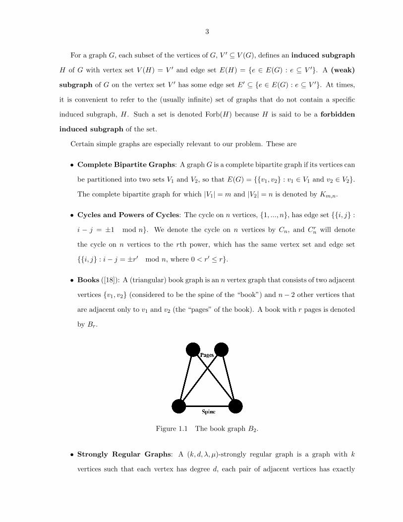
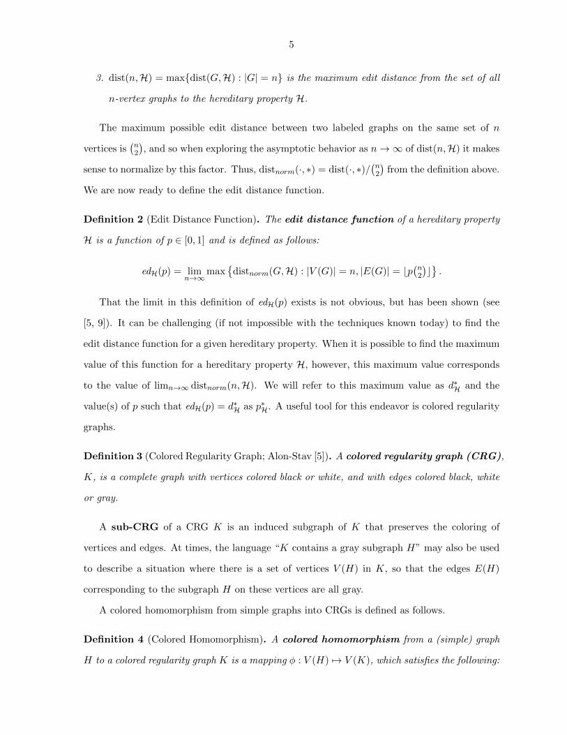
• Books ([18]): A (triangular) book graph is an n vertex graph that consists of two adjacent

vertices {v1, v2} (considered to be the spine of the “book”) and n− 2 other vertices that

are adjacent only to v1 and v2 (the “pages” of the book). A book with r pages is denoted

by Br.

Figure 1.1 The book graph B2.

• Strongly Regular Graphs: A (k, d, λ, µ)-strongly regular graph is a graph with k

vertices such that each vertex has degree d, each pair of adjacent vertices has exactly

4

λ neighbors in common, and each pair of nonadjacent vertices has exactly µ common

neighbors. It should be noted that this notation for parameters is somewhat unorthodox,

but was selected to be consistent with notation for colored regularity graphs discussed

later in this section.

Certain graphs constructed by Zoltan Furedi [29] will also play a key role in our exploration

the edit distance function later in this paper. These graphs are discussed in Sections 2.5.3 and

3.2.

1.1.2 Terminology and notation specific to the problem

The edit distance functions explore the asymptotic maximum normalized edit distance from

specific graph properties. In particular, they are well-defined for a subset of graph properties

called hereditary graph properties. A hereditary graph property, H, is a set of graphs

that is closed under both isomorphism and vertex deletion. Any hereditary graph property

can always be described by a (possibly infinite) set of forbidden induced subgraphs. A

convenient subset of hereditary properties is the properties that can be completely defined by

forbidding a single induced subgraph. These are called principle hereditary properties,

and as mentioned above, each may be denoted by Forb(H), where H is the forbidden induced

subgraph that completely defines the property. The results in this thesis pertain to the principle

hereditary properties described by Forb(K2,t) (e.g., Forb(K2,3), Forb(K2,4), Forb(K2,5), etc.).

The edit distance between two graphs G and G′ may be described as the minimum number

of edge changes (either additions or deletions) necessary to make a graph G the same as G′,

and this idea can be extended to describe the edit distance from G to an entire set of graphs.

Here we rigorously define these notions of graph edit distance.

Definition 1 (Edit Distance). Let G and H be simple graphs on the same labeled vertex set,

and let H be a hereditary property, then

1. dist(G,H) = |E(G)∆E(H)| is the edit distance from G to H,

2. dist(G,H) = min{dist(G,H) : H ∈ H and V (G) = V (H)} is the edit distance from G to

H and

5

3. dist(n,H) = max{dist(G,H) : |G| = n} is the maximum edit distance from the set of all

n-vertex graphs to the hereditary property H.

The maximum possible edit distance between two labeled graphs on the same set of n

vertices is(n2

), and so when exploring the asymptotic behavior as n→∞ of dist(n,H) it makes

sense to normalize by this factor. Thus, distnorm(·, ∗) = dist(·, ∗)/(n2

)from the definition above.

We are now ready to define the edit distance function.

Definition 2 (Edit Distance Function). The edit distance function of a hereditary property

H is a function of p ∈ [0, 1] and is defined as follows:

edH(p) = limn→∞

max{

distnorm(G,H) : |V (G)| = n, |E(G)| = bp(n2

)c}.

That the limit in this definition of edH(p) exists is not obvious, but has been shown (see

[5, 9]). It can be challenging (if not impossible with the techniques known today) to find the

edit distance function for a given hereditary property. When it is possible to find the maximum

value of this function for a hereditary property H, however, this maximum value corresponds

to the value of limn→∞ distnorm(n,H). We will refer to this maximum value as d∗H and the

value(s) of p such that edH(p) = d∗H as p∗H. A useful tool for this endeavor is colored regularity

graphs.

Definition 3 (Colored Regularity Graph; Alon-Stav [5]). A colored regularity graph (CRG),

K, is a complete graph with vertices colored black or white, and with edges colored black, white

or gray.

A sub-CRG of a CRG K is an induced subgraph of K that preserves the coloring of

vertices and edges. At times, the language “K contains a gray subgraph H” may also be used

to describe a situation where there is a set of vertices V (H) in K, so that the edges E(H)

corresponding to the subgraph H on these vertices are all gray.

A colored homomorphism from simple graphs into CRGs is defined as follows.

Definition 4 (Colored Homomorphism). A colored homomorphism from a (simple) graph

H to a colored regularity graph K is a mapping φ : V (H) 7→ V (K), which satisfies the following:

6

1. If uv ∈ E(H), then either φ(u) = φ(v) = m and m is colored black, or φ(u) 6= φ(v) and

the edge φ(u)φ(v) is colored black or gray.

2. If uv /∈ E(H), then either φ(u) = φ(v) = m and m is colored white, or φ(u) 6= φ(v) and

the edge φ(u)φ(v) is colored white or gray.

A colored homomorphism from a simple graph H to a CRG K is sometimes referred to as

an embedding of H in K. If no such homomorphism exists for a particular graph H, we say

that K forbids H embedding.

As in [9], the sets of white vertices, white edges, black vertices, and black edges are denoted

VW(K), EW(K),VB(K), and EB(K) respectively for a given CRG K, and two functions of p

are defined as follows:

fK(p) =1

k2[p(|VW(K)|+ 2|EW(K)|) + (1− p)(|VB(K)|+ 2|EB(K)|)] (1.1)

gK(p) = min{uTMK(p)u : uT1 = 1 and u ≥ 0}. (1.2)

Here MK(p) denotes a weighted adjacency matrix assigning a weight of p to the ijth entry

if the edge {i, j} in the CRG is white or if i = j and the vertex corresponding to i is white, and

a weight of (1−p) if the edge {i, j} in the CRG is black or if i = j and the vertex corresponding

to i is black. If the edge {i, j} is gray, then the corresponding value is 0. The significance of

these two functions (as shown in [9]) is that

edH(p) = inf fK(p) = inf gK(p)

where inf is taken over all of the CRGs K that permit the embedding of graphs in H only.

Definition 5 (p-core CRG). A p-core CRG is a CRG K ′ such that for no nontrivial sub-CRG

K of K ′ is it the case that gK(p) = gK′(p). In other words, if K ′ is a p-core CRG, and K is a

nontrivial sub-CRG of K ′, then gK(p) > gK′(p).

For p-core CRGs K, it is shown in [32] that there is a unique vector x such that xT1 =

1 and x ≥ 0, and gK(p) = xTMK(p)x. This vector x can be viewed as a function of the vertices

7

v ∈ V (K), so that x(v) is the weight that x assigns to the vertex v. It is referred to in the

literature as the optimal weight function of K at p. With such a weight function in place,

we will also need the value dG(v), which is the sum of the weights of vertices adjacent to v in

K via gray edges.

Some important CRG constructions for Forb(K2,t) are defined (as in [34]) below.

Definition 6. Let K(w, b) denote the CRG with w white vertices, b black vertices and only

gray edges. In particular:

1. Let K(1, 1) be the CRG consisting of a white and black vertex joined by a gray edge.

2. Let K(0, t− 1) be the CRG consisting of t− 1 black vertices all joined by gray edges.

1.2 Select review of the literature and past results

Recent papers by Axenovich et al. [7] and Alon and Stav [5] originated current interest in

the determination of bounds for dist(n,H).

The work of Axenovich et al. cites applications of graph editing problems to computer

science and bioinformatics, in particular work by Chen et al. in [17], as practical motivations

for their work. As is pointed out in both [7] and [5], these types of problems are a one of several

natural evolutions of Turan type problems [20, 22, 23, 24, 26, 27, 28], as well as other editing

problems, especially those involving more global properties [8, 21].

Their results make use of the so-called binary chromatic number to bound the maximum

possible edit distance of any graph from a principle hereditary property H = Forb(H). The

binary chromatic number, introduced by Promel and Steger in [37] as the parameter τ and

generalized in [13], is defined in [7] as follows:

Definition 7 (Binary Chromatic Number). The binary chromatic number of a graph G, χB(G)

is the least integer k + 1 such that, for all c ∈ {0, ..., k + 1}, there exists a partition of V (G)

into c cliques and k + 1− c cocliques.

In [7], they also define cmin to be the least value of c that does not allow G to be partitioned

into c cliques and k− c cocliques, and cmax be the greatest value of c that does not allow such a

8

partition, where k = χB(G)− 1. What follows is a summary of some of their results bounding

dist(n,Forb(H)) using these parameters.

Theorem 8 (Axenovich et al. [7]). If H is a graph with binary chromatic number k + 1, then

dist(n,Forb(H)) > (1− o(1))n2

4k

Theorem 9 (Axenovich et al. [7]). Let H be a graph with binary chromatic number k + 1. If

cmin ≤ k/2 ≤ cmax then

dist(n,Forb(H)) ≤ 1

2k

(n

2

).

Combining these two bounds on dist(n,Forb(H) yielded the following nice result for self-

complementary H.

Corollary 10 (Axenovich et al. [7]). If H is a self-complementary graph with the property

that χB(H) = k + 1, then

dist(n,Forb(H)) = (1 + o(1))n2

4k.

In addition, they determined dist(n,Forb(H)) for H ∈ {K3,K3,K1,2,K1,2}, and bounded

dist(n,Forb(H)) in several other cases.

Meanwhile in [5], Alon and Stav cite algorithmic edge-modification problems in theoretical

computer science as a key motivation for their exploration of the problem. Their approach

uses several versions of the regularity lemma [2, 31, 39] and colored regularity graph structures

(originated by Bollobas and Thomason in [13]). It follows a method, used by Alon and Shapira

in [3] to address questions about edit distance and property testing, to achieve their main

result:

Theorem 11 (Alon and Stav [5]). Let H be an arbitrary hereditary graph property. Then there

exists p∗ ∈ [0, 1], such that with high probability

dist(n,H) = dist(G(n, p∗),H) + o(n2).

In the case of self-complementary graphs addressed in Corollary 10, it has been observed

that p∗ = 1/2 for the above theorem. In general, however, the p∗ for a specific hereditary

9

property is not determined explicitly by the proof of Theorem 11, and in fact, as will be

discussed later in this thesis, for some hereditary properties an interval of p∗ values may work.

An approach to finding p∗, employed by Balogh and Martin in [9], is to calculate the

expected value of limn→∞ distnorm(G(n, p),H) for all p ∈ [0, 1], and then find the value(s) of

p that yield the maximum distance. What follows is the main result from their work. Recall

that fK(p) and gK(p) are defined by equations 1.1 and 1.2.

Theorem 12 (Balogh and Martin [9]). For a hereditary property H, let K(H) denote all CRGs

K that do not permit the embedding of any of the forbidden induced subgraphs associated with

H. Then d∗(H) = limn→∞ distnorm(n,H) exists. Define

f(p) = infK∈K(H)

fK(p) and g(p) = infK∈K(H)

gK(p).

Then it is the case that f(p) = g(p) for all p ∈ [0, 1],

d∗H = maxp∈[0,1]

f(p) = maxp∈[0,1]

g(p),

and p∗H is the value of p at which f achieves its maximum. In addition, the function f(p) = g(p)

is concave.

Furthermore, for all p ∈ (0, 1),

maxG:|E(G)|=p(n2)

{dist(G,H)} = f(p)

(n

2

)+ o(n2),

and for all ε > 0, dist(G(n, p),H) ≥ f(p)(n2

)− εn2.

This theorem tells us not only that edH(p) is well defined for all p, but that it is actually

achieved for each p by limn→∞ E[distnorm(G(n, p),H)], where fK(p) and gK(p) can be viewed

as two different approaches to find this quantity. The observed concavity of the function is

a helpful tool for determining its maximum, even when the entire function is not computable

(which, at least with current techniques, is often the case).

Furthermore, while p∗ and d∗ were determined by Alon and Stav in [4] for H = Forb(H)

when V (H) ≤ 4, the methods used in [9] to determine these parameters with the edit distance

10

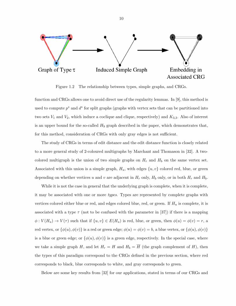
Figure 1.2 The relationship between types, simple graphs, and CRGs.

function and CRGs allows one to avoid direct use of the regularity lemmas. In [9], this method is

used to compute p∗ and d∗ for split graphs (graphs with vertex sets that can be partitioned into

two sets V1 and V2, which induce a coclique and clique, respectively) and K3,3. Also of interest

is an upper bound for the so-called H9 graph described in the paper, which demonstrates that,

for this method, consideration of CRGs with only gray edges is not sufficient.

The study of CRGs in terms of edit distance and the edit distance function is closely related

to a more general study of 2-coloured multigraphs by Marchant and Thomason in [32]. A two-

colored multigraph is the union of two simple graphs on Hr and Hb on the same vertex set.

Associated with this union is a simple graph, Hu, with edges {u, v} colored red, blue, or green

depending on whether vertices u and v are adjacent in Hr only, Hb only, or in both Hr and Hb.

While it is not the case in general that the underlying graph is complete, when it is complete,

it may be associated with one or more types. Types are represented by complete graphs with

vertices colored either blue or red, and edges colored blue, red, or green. If Hu is complete, it is

associated with a type τ (not to be confused with the parameter in [37]) if there is a mapping

φ : V (Hu) → V (τ) such that if {u, v} ∈ E(Hu) is red, blue, or green, then φ(u) = φ(v) = r, a

red vertex, or {φ(u), φ(v)} is a red or green edge; φ(u) = φ(v) = b, a blue vertex, or {φ(u), φ(v)}

is a blue or green edge; or {φ(u), φ(v)} is a green edge, respectively. In the special case, where

we take a simple graph H, and let Hr = H and Hb = H (the graph complement of H), then

the types of this paradigm correspond to the CRGs defined in the previous section, where red

corresponds to black, blue corresponds to white, and gray corresponds to green.

Below are some key results from [32] for our applications, stated in terms of our CRGs and

11

edit distance functions. For more information on 2-coloured multigraphs, the reader may wish

to consult [40], an excellent survey by Thomason of the topic, including its applications to edit

distance.

Theorem 13 (Marchant and Thomason [32]). Let K be a p-core CRG. Then all edges of K

are gray, except

• if p < 1/2, then some edges joining two black vertices might be white, or

• if p > 1/2, then some edges joining two white vertices might be black.

While lower bounds in [9] came mainly from f(p), Theorem 13 lays the foundation for

developing lower bounds using g(p). What is more, Marchant and Thomason show that, in fact,

infK∈K(H) gK(p) = minK∈K(H) gK(p). Through examples, they also demonstrate the following

partial results for H = Forb(K2,t).

Theorem 14 (Lemma 5.14 and Example 5.16 in Marchant and Thomason [32]). Let H =

Forb(K2,t), then

• if t = 2, edH(p) = p(1− p).

• any CRG K with all black vertices and only white and gray edges so that the gray subgraph

does not have K2,t or the book Bt−1 forbids K2,t embedding.

• if p ≥ 1/2 then for t > 2, edH(p) = 1−pt−1

• if p ≤ 1/2 then for t > 2, either edH(p) = min{p(1−p), 1−pt−1 } or edH(p) = gK(p) for some

CRG K ∈ K(H) that has no white vertices.

In the above theorem, the bound of p(1 − p) comes from the CRG K(1, 1) and the bound

1−pt−1 from K(0, t− 1).

Theorem 15 pertains to the value of gK(p) for certain CRGs with regular gray subgraphs.

Theorem 15 (Marchant and Thomason [32]). Let d ≥ 2 be an integer and let G be a connected

d-regular graph of order n. Let K be the CRG with vertex set V (G) whose vertices are all black,

with the edges of G colored gray and all other edges white.

If p ≤ 1/(d+ 2) then K is p-core, and gK(p) = 1k +

(k−d−2k

)p.

12

This result is interesting because many of the CRG constructions in this thesis are, in fact,

regular. In this case fK(p) = 1k +

(k−d−2k

)p as well, and so it appears to be the case that at

least for smaller values of p, an even weighting in such instances is optimal for gK(p).

In addition to these results, Marchant and Thomason consider several other examples per-

taining to hereditary properties, including an alternative example to H9 in [9] for a property

that requires CRGs that do not have all gray edges to determine the maximum value of its edit

distance function, and an example of properties that have an infinite number of p-core CRGs

K, such that for some fixed p, edH(p) = gK(p). This last example pertains to questions of

the stability of structures within a property that are likely to be closest to the random graph

G(n, p), a question that is also explored for the case when p = 1/2 by Alon and Stav in [6].

A final example from Marchant and Thomason that was of particular interest for this thesis

was an application of a dense bipartite K3,3-free graph construction by Brown in [16], where in

this case, K3,3-free refers to the absence of a weak K3,3 subgraph, to improve on other bounds

for this construction for small p.

Such constructions for Ks,t-free graphs in general are closely related to the Zarankiewicz

problem, which asks how many edges can a graph on n vertices have before it must contain a

Ks,t subgraph. Bipartite versions of these constructions can naturally be converted into CRGs

that forbid K2,t embedding, and so one question addressed in [34] that is also discussed in this

thesis, is what similar constructions by Furedi in [29] mean for edForb(K2,t)(p).

In addition to these constructions for a classic extremal graph theory question, we also look

at CRG constructions inspired by known strongly regular graphs as summarized at Brouwer’s

website [15] and variations on triangle free cycle constructions discussed by Brandt in [14].

Two other results that are essential to establishing lower bounds for the edit distance

functions of Forb(K2,t) appears as lemmas in [33].

Lemma 16 (Martin [33]). Let p ∈ (0, 1) and K be a p-core CRG with optimal weight function

x.

1. If p ≤ 1/2, then x(v) = gK(p)/p for all v ∈ VW(K) and

dG(v) =p− gK(p)

p+

1− 2p

px(v), for all v ∈ VB(K).

13

2. If p ≥ 1/2, then x(v) = gK(p)/(1− p) for all v ∈ VB(K) and

dG(v) =1− p− gK(p)

1− p+

2p− 1

1− px(v), for all v ∈ VW(K).

Lemma 17 (Martin [33]). Let p ∈ (0, 1) and K be a p-core CRG with optimal weight function

x.

1. If p ≤ 1/2, then x(v) ≤ gK(p)/(1− p) for all v ∈ VB(K).

2. If p ≥ 1/2, then x(v) ≤ gK(p)/p for all v ∈ VW(K).

As is evident from Theorem 14, the case when p ≤ 1/2 is of most interest for our purposes.

However, the main results of [33] include bounds on the edit distance function for any heredi-

tary properties that forbid a clique, and exact determination of the edit distance function for

principal hereditary properties defined by forbidding Kn, Cn when n ≤ 9, and C10 for p ≥ 1/7,

with a resulting determination of p∗ and d∗ for each of these principal hereditary properties.

In addition to the recent work on edit distance and the edit distance function summarized

above, a number of related questions have also been asked. For instance, how many graphs

of order n are are there in a specific hereditary property [37, 38], and what is the probability

that the random graph G(n, p) does, in fact, fall in a hereditary property [1] (see also [11],

[12], [35],[36] for additional work on hereditary properties and forbidden induced subgraphs)?

Exploration in these areas helped lay the foundation for this more recent work.

1.3 Results

The following results from [34] (joint work with Ryan Martin) will be discussed in Chapter

2.

Theorem 18. Let H = Forb(K2,3). Then edH(p) = min{p(1 − p), 1−p2 } with p∗H = 12 and

d∗H = 14 .

Theorem 19. Let H = Forb(K2,4). Then edH(p) = min{p(1− p), 7p+115 , 1−p3 } with p∗H = 1

3 and

d∗H = 29 .

14

It should be noted that the values of these functions for when p ≥ 1/2 from Theorems 18

and 19 follow directly from Theorem 14. The function value of 1−pt−1 for p ≥ 1/2 in Theorem 14

from [32] are extended for general t below.

Theorem 20. Let t ≥ 4, p ≥ 2/(t+ 1) and H = Forb(K2,t), then edH(p) = (1− p)/(t− 1).

Theorem 21. Let t ≥ 3 and p < 1/2. If K is a black-vertex, p-core CRG with white and gray

edges such that the gray edges have neither a K2,t nor a book Bt−2, then

gK(p) ≥ p− t− 1

4t− 5

[3p− 2 + 2

√1− 3p+ (t+ 1)p2

]. (1.3)

Theorem 22. For odd t ≥ 5 and H = Forb(K2,t),

d∗H = 1/(t+ 1) and p∗H ⊇[

2t− 1

t(t+ 1),

2

t+ 1

].

Theorem 22 is the first principal hereditary property known to have a nondegenerate interval

of possible values for p∗.

The next two results follow from constructions by Furedi [29].

Theorem 23. For H = Forb(K2,t), the edit distance function edH(p) ≤ t−1+p(2q2−q(t−1)−2t)2(q2−1)

for any prime power q such that t− 1 divides q − 1.

Corollary 24. For t ≥ 9, there exists a value q0, so that if q > q0, then t−1+p(2q2−q(t−1)−2t)2(q2−1) <

p(1 − p) for some values of p, which approach 0 as q increases. That is, arbitrarily close to

p = 0, there is some value for p such that edH(p) < p(1− p).

A strongly regular graph construction provides the upper bound 7p+115 for edForb(K2,4)(p).

Such constructions continue to be relevant for larger t values, and so we have the following

general result for such graphs.

Theorem 25. For any (k, d, λ, µ)-strongly regular graph, there exists a corresponding CRG,

K, such that

fK(p) =1

k+

(k − d− 2

k

)p.

If λ ≤ t− 3 and µ ≤ t− 1, then K forbids K2,t embedding, and when equality holds for both λ

and µ,

fK(p) =t− 1

t− 1 + d(d+ 1)+

(1− (d+ 2)(t− 1)

t− 1 + d(d+ 1)

)p. (1.4)

15

There is an interesting connection between strongly regular graphs and the lower the result

in Theorem 21. Namely, the upper bound resulting from a (k, d, t − 3, t − 1)-strongly regular

graph is always a line tangent to this lower bound.

The following general upper bound arises from a CRG construction involving the second

power of cycles. The reasoning for our attention to these particular cycle powers will be

discussed further in Chapter 3.

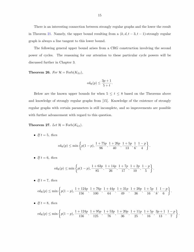
Theorem 26. For H = Forb(K2,t),

edH(p) ≤ 3p+ 1

5 + t.

Below are the known upper bounds for when 5 ≤ t ≤ 8 based on the Theorems above

and knowledge of strongly regular graphs from [15]. Knowledge of the existence of strongly

regular graphs with certain parameters is still incomplete, and so improvements are possible

with further advancement with regard to this question.

Theorem 27. Let H = Forb(K2,t).

• If t = 5, then

edH(p) ≤ min

{p(1− p), 1 + 75p

96,1 + 26p

40,1 + 5p

13,1

6,1− p

4

}.

• If t = 6, then

edH(p) ≤ min

{p(1− p), 1 + 63p

85,1 + 14p

26,1 + 7p

17,1 + 2p

10,1− p

5

}.

• If t = 7, then

edH(p) ≤ min

{p(1− p), 1 + 124p

156,1 + 76p

100,1 + 44p

64,1 + 31p

49,1 + 20p

36,1 + 5p

16,1

8,1− p

6

}.

• If t = 8, then

edH(p) ≤ min

{p(1− p), 1 + 124p

156,1 + 95p

125,1 + 53p

76,1 + 20p

36,1 + 11p

25,1 + 5p

16,3p+ 1

13,1− p

7

}.

16

CHAPTER 2. PROOFS FOR RESULTS FROM [34]

This chapter contains proofs of the results from Section 1.3 that also appear in [34], a joint

work with Ryan Martin. While most of the arguments appear as they were written in sections

3-7 and the appendices of the paper, there is some modifications from the original text for the

sake of clarity and continuity.

2.1 Preliminary results and observations

We begin with some notation used throughout the chapter.

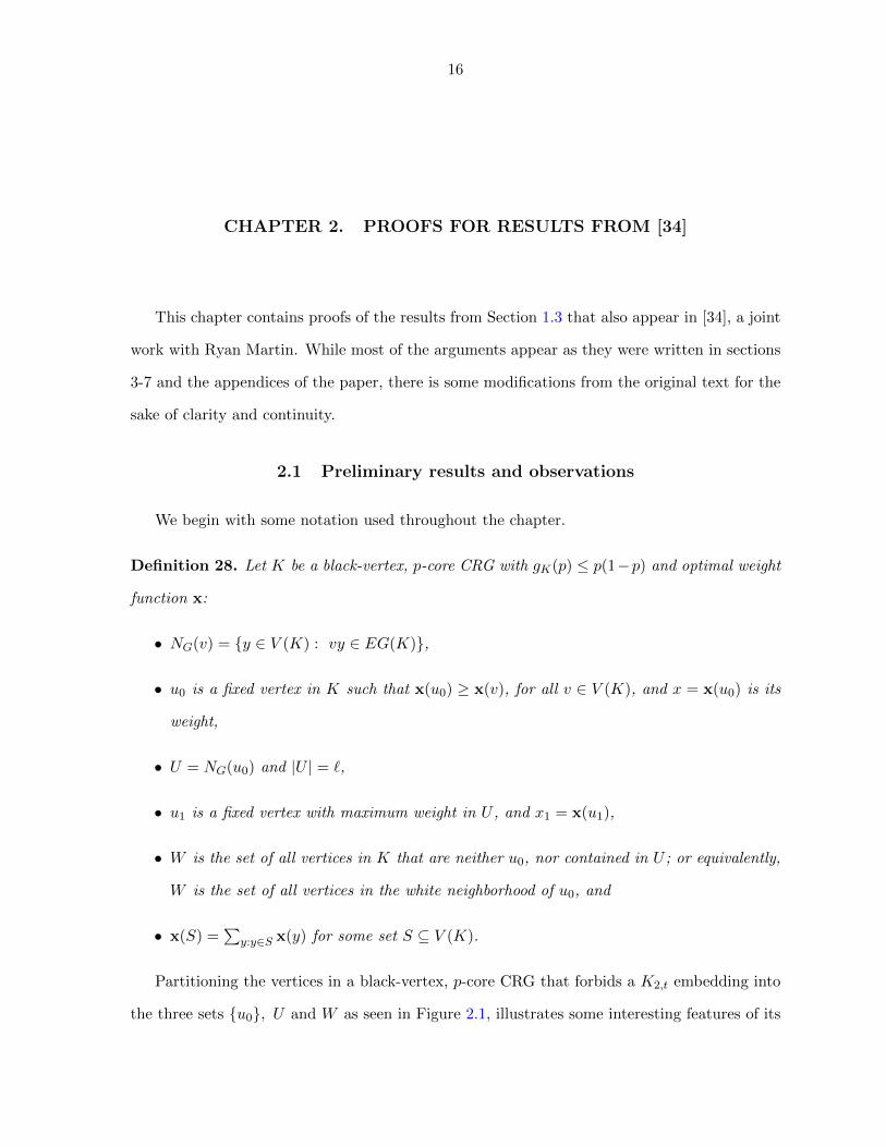
Definition 28. Let K be a black-vertex, p-core CRG with gK(p) ≤ p(1−p) and optimal weight

function x:

• NG(v) = {y ∈ V (K) : vy ∈ EG(K)},

• u0 is a fixed vertex in K such that x(u0) ≥ x(v), for all v ∈ V (K), and x = x(u0) is its

weight,

• U = NG(u0) and |U | = `,

• u1 is a fixed vertex with maximum weight in U , and x1 = x(u1),

• W is the set of all vertices in K that are neither u0, nor contained in U ; or equivalently,

W is the set of all vertices in the white neighborhood of u0, and

• x(S) =∑

y:y∈S x(y) for some set S ⊆ V (K).

Partitioning the vertices in a black-vertex, p-core CRG that forbids a K2,t embedding into

the three sets {u0}, U and W as seen in Figure 2.1, illustrates some interesting features of its

17

optimal weight function when the gray neighborhoods of these vertices are considered in the

context of Lemma 16. One such feature is the upper bounds in Proposition 29 for x1.

Figure 2.1 A partition of the vertices in a black-vertex, p-core CRG, K. Dashed lines and graybackground represent gray edges. White edges are omitted, as are edges withinsubsets.

Proposition 29. Let K ∈ [K(Forb(K2,3)) ∪ K(Forb(K2,4))] be a black-vertex, p-core CRG. If

either p < 1/3 or both p < 1/2 and the gray sub-CRG of K is triangle-free, then

x1 ≤ x and x1 ≤ p− x

where x = x(u0) is the maximum weight of a vertex in K, and x1 = x(u1) is the maximum

weight of a vertex in that vertex’s gray neighborhood.

Proof. The inequality x1 ≤ x follows directly from definitions of x1 and x, since x is the greatest

weight in K. To justify the inequality x1 ≤ p− x, we break the problem into two cases:

Case 1: u0 and u1 have no common gray neighbor.

Recall that u1 is a vertex with maximum weight in the gray neighborhood of u0, a vertex

with maximum weight in all of K, and assume that x+ x1 > p. Then applying Lemma 16 and

Theorem 14,

dG(u0) + dG(u1) ≥[p+

1− 2p

px

]+

[p+

1− 2p

px1

]= 2p+

(1− 2p

p

)(x+x1) > 2p+ (1− 2p).

18

This is a contradiction because in Case 1, NG(u0)∩NG(u1) = ∅. Thus, dG(u0)+dG(u1) ≤ 1,

since the sum of the weights of the vertices in K must be 1.

This completes the proof of Proposition 29 for K ∈ K(Forb(K2,3)), since, in this case, no

K ∈ K contains a gray triangle (book B1). So we may assume that K ∈ K(Forb(K2,4)).

Case 2: u0 and u1 have a common gray neighbor and p < 1/3.

In this case, u1 has a single neighbor u2 in U because any more such neighbors would result

in a gray book B2 (contradicting Theorem 14). Furthermore, we note that in order to avoid

a gray book B2, the common neighborhood of u1 and u2 in W must be empty. Consequently,

dG(u1) + dG(u2) ≤ x(W ) + 2x+ x1 + x(u2).

Applying similar reasoning to that in Case 1,

dG(u0) + dG(u1) + dG(u2) ≥[p+

1− 2p

px

]+

[p+

1− 2p

px1

]+

[p+

1− 2p

px(u2)

].

So,

dG(u0) + (x(W ) + 2x+ x1 + x(u2)) ≥[p+

1− 2p

px

]+

[p+

1− 2p

px1

]+

[p+

1− 2p

px(u2)

]x(U) + (x(W ) + 2x+ x1 + x(u2)) ≥ 3p+

1− 2p

p(x+ x1 + x(u2))

x(U) + x(W ) + x ≥ 3p+1− 3p

p(x+ x1 + x(u2))

1 ≥ 3p+1− 3p

p(x+ x1 + x(u2)) .

With p < 1/3 and x+ x1 ≥ p, we have a contradiction.

Applying the pigeon-hole principle, we also have the following lower bound for `:

Fact 30. In a CRG, if u0 is a vertex with maximum weight, x = x(u0), the maximum weight

in the gray neighborhood of u0 is x1, and the order of the gray neighborhood of u0 is `, then

` ≥ dG(u0)/x1 ≥ dG(u0)/x.

19

While simple, when combined with Lemma 16 and Proposition 29 along with the observation

that x(u0) + x(U) + x(W ) = 1, this fact forces a balance between the weights of the vertex u0,

the vertices in U , and the vertices in W , that is a powerful tool for bounding gK(p).

2.2 Proof of Theorem 18

In this section, we establish the value of edForb(K2,3)(p) for p ∈ (0, 1/2), determining the

entire function via continuity and Theorem 14, from which we know that edForb(K2,3)(p) =

(1− p)/2 for p ∈ [1/2, 1].

For the following discussion, we will assume that K is a p-core CRG on all black vertices

into which K2,3 may not be embedded and that gK(p) ≤ p(1− p). The following lemma yields

a useful restriction of the order of U .

Lemma 31. Let K be a black-vertex, p-core CRG with p ∈ (0, 1/2), no gray triangles, no gray

K2,3 and gK(p) ≤ p(1 − p). If u0 is a vertex of maximum weight, x, in K, and ` = |NG(u0)|,

then

` ≤2(1− x)− 1

pdG(u0)

p− x.

Proof. Let u1, . . . , u` be an enumeration of the vertices in U , the gray neighborhood of u0.

Observe that K cannot contain a K3 with all gray edges, and so U contains no gray edges.

Therefore, with the exception of u0, the entire gray neighborhood of each ui is contained in

W . Furthermore, if any three vertices in U had a common gray neighbor in W , then K would

contain a gray K2,3. That is, each vertex in W is adjacent to at most two vertices in U via a

gray edge. Applying these observations,

∑i=1

(dG(ui)− x) ≤ 2x(W ).

Using Lemma 16 and the assumption that p−gK(p)p ≥ p,

∑i=1

(p− x+

1− 2p

px(ui)

)≤ 2x(W ).

20

The fact that x(W ) = 1− x− dG(u0), gives

`(p− x) +1− 2p

pdG(u0) ≤ 2 (1− x− dG(u0))

`(p− x) ≤ 2− 2x− 1

pdG(u0)

` ≤2(1− x)− 1

pdG(u0)

p− x.

The following technical lemma is an important tool in the proof of Theorem 18.

Lemma 32. Let K be a black-vertex, p-core CRG for p ∈ (0, 1/2) with no gray triangles, no

gray K2,3 and gK(p) ≤ p(1− p). If x and x1 are defined as in Proposition 29, then[p+

1− 2p

px

] [1

x1+

1

p(p− x)

]≤ 2(1− x)

p− x.

Proof. By Fact 30, ` ≥ dG(u0)x1

, and by Lemma 31, ` ≤2(1−x)− 1

pdG(u0)

p−x . Therefore,

dG(u0)

x1≤

2(1− x)− 1pdG(u0)

p− x.

After combining the dG(u0) terms we get,

dG(u0)

[1

x1+

1

p(p− x)

]≤ 2(1− x)

p− x,

and then applying Lemma 16,[p+

1− 2p

px

] [1

x1+

1

p(p− x)

]≤ 2(1− x)

p− x.

Proof of Theorem 18. Let p ∈ (0, 1/2), and K be a black-vertex, p-core CRG with gK(p) <

p(1− p) and no gray triangle (i.e., the book B1) or gray K2,3.

With the above assumptions, we will show that there is no possible value for x, the value

of the largest vertex-weight. To do so, we break the problem into 2 cases: x ≥ p2 and x < p

2 .

Case 1: x ≥ p/2.

21

We start with the inequality from Lemma 32,[p+

1− 2p

px

] [1

x1+

1

p(p− x)

]≤ 2(1− x)

p− x,

and apply the bound x1 ≤ p− x from Proposition 29 to get[p+

1− 2p

px

] [1

p− x+

1

p(p− x)

]≤ 2(1− x)

p− x.

From Lemma 17, p− x > 0, and so[p+

1− 2p

px

] [1 +

1

p

]≤ 2(1− x)

x

(1− pp2

)≤ 1− p

x ≤ p2,

a contradiction, since p2 > p2 for p ∈ (0, 1/2).

Case 2: x < p/2.

We again apply Lemma 32, only now we employ the trivial bound x1 ≤ x from Proposition

29:

[p+

1− 2p

px

] [1

x+

1

p(p− x)

]≤ 2(1− x)

p− x[p+

1− 2p

px

][p(p− x) + x] ≤ 2px(1− x)

(4p2 − 3p+ 1)x2 − (3p3)x+ p4 ≤ 0.

Observe that 4p2− 3p+ 1 is always positive, and therefore the parabola (4p2− 3p+ 1)x2−

(3p3)x+ p4, in the variable x, is concave up, so the range of x values for which this inequality

is satisfied is x ∈ [x′, x′′] where

22

x′ =3p3 −

√−4p4 + 12p5 − 7p6

2(1− 3p+ 4p2)and x′′ =

3p3 +√−4p4 + 12p5 − 7p6

2(1− 3p+ 4p2).

If p < (6 − 2√

2)/7, then neither x′ nor x′′ is real, and so the inequality is never satisfied.

For p ∈[6−2√2

7 , 12

), routine calculations show that p

2 < x′, a contradiction to the assumption

that x < p2 .

Hence, there is no possible value for x if edForb(K2,3)(p) < p(1− p), so the proof is complete.

2.3 Proof of Theorem 19

This section addresses the case of edForb(K2,4)(p).

2.3.1 Upper bounds

Recall that from Theorem 14 we already know that edForb(K2,4)(p) ≤ min{p(1 − p), 1−p3 }.

For the remaining upper bound, we turn to strongly regular graphs.

Lemma 33. Let H = Forb(K2,t). If there exists a (k, d, λ, µ)-strongly regular graph with

λ ≤ t− 3 and µ ≤ t− 1, then

edH(p) ≤ 1

k+k − d− 2

kp.

Proof. Let G be the aforementioned strongly regular graph. We construct a CRG, K, on k

black vertices with gray edges in K corresponding to adjacent vertices in G and white edges in

K corresponding to nonadjacent vertices in G.

No pair of adjacent vertices has t − 2 > λ common neighbors, so there is no book Bt−2 in

the gray subgraph, and no pair of vertices has t > µ, λ common neighbors, so there is no K2,t

in the gray subgraph. Thus, by Theorem 14, K forbids K2,t embedding. Furthermore,

fK(p) =1

k2

[(1− p)k + 2p

((k

2

)− dk

2

)]=

1

k+k − d− 2

kp.

23

In fact, there is a (15, 6, 1, 3)-strongly regular graph [15]. It is a so-called “generalized

quadrangle,” GQ(2, 2). As a result,

edForb(K2,4)(p) ≤ min

{p(1− p), 1 + 7p

15,1− p

3

}.

2.3.2 Lower bounds

Because the edit distance function is both continuous and concave down, it is sufficient to

verify that edForb(K2,4)(p) ≥ p(1 − p) for p ∈ (0, 1/5) and that edForb(K2,4)(p) ≥ (1 − p)/3 for

p ∈ (1/3, 1/2). This is because the line determined by the bound 1+7p15 passes through the

points (1/5, 4/25) and (1/3, 2/9). Furthermore, by Theorem 14, we need only consider CRGs

that have black vertices and white and gray edges.

Lemmas 34 and 37 address the cases where p ∈ (1/3, 1/2) and where p ∈ (0, 1/5), respec-

tively.

Lemma 34. Let p ∈ (1/3, 1/2). If K is a black-vertex, p-core CRG that does not contain a

gray book B2 or a gray K2,4, then gK(p) ≥ 1−p3 , with equality occurring only if K is a gray

triangle (i.e., K ≈ K(0, 3)).

Proof. We break this into two cases: when K does and does not have a gray triangle.

Case 1: K has a gray triangle.

Let the gray subgraph of K contain a triangle whose vertices are v1, v2 and v3 with optimal

weights y1, y2 and y3, respectively. Because K has no gray B2, we know that no pair of the

vertices v1, v2, v3 have a common gray neighbor other than the remaining vertex in the triangle.

Letting g = gK(p), we have the following because the sum of the optimal weights on all vertices

in K is 1:

y1 + y2 + y3 +3∑i=1

[dG(vi)− (y1 + y2 + y3 − yi)] ≤ 1.

24

Then, applying Lemma 16,

y1 + y2 + y3 + 3

(p− gp

)+

1− 2p

p(y1 + y2 + y3)− 2(y1 + y2 + y3) ≤ 1

3

(p− gp

)+

1− 3p

p(y1 + y2 + y3) ≤ 1,

and so

2p− 3g

p≤

(3p− 1

p

)(y1 + y2 + y3) ≤

3p− 1

p.

Consequently, g ≥ (1− p)/3 with equality if and only if y1 + y2 + y3 = 1; i.e., K itself is a

gray triangle.

Case 2: K has no gray triangle.

Let u0 be a vertex of largest weight, x = x(u0), and let U = NG(u0). The absence of a

gray triangle means that there are no gray edges between pairs of vertices in U . Furthermore,

no vertex in W can be adjacent to more than three vertices in U via a gray edge, since by

Theorem 14, the gray subgraph of K does not contain a K2,4.

Let u1, . . . , u` be an enumeration of the vertices in U with weights x1, . . . , x`, respectively,

and g = gK(p). Then

∑i=1

(dG(ui)− x) ≤ 3x(W )

≤ 3(1− x− x(U)),

and applying Lemma 16 to compute dG(ui),

∑i=1

(p− gp

+1− 2p

pxi − x

)≤ 3(1− x− x(U))

`

(p− gp− x)

+1− 2p

px(U) ≤ 3(1− x)− 3x(U)

`

(p− gp− x)≤ 3(1− x)− 1 + p

px(U). (2.1)

First, suppose ` ≥ 5. Then, from inequality (2.1), we have

5

(p− gp− x)≤ 3(1− x)− 1 + p

px(U),

25

and applying Lemma 16 again,

5

(p− gp− x)≤ 3(1− x)− 1 + p

p

(p− gp

+1− 2p

px

)1 + 6p

p· p− g

p− 3 ≤

(5− 3− 1 + p

p· 1− 2p

p

)x

p(1 + 3p)− g(1 + 6p) ≤ x(4p2 + p− 1

).

If 4p2 + p− 1 < 0, then we may use the fact that x > 0,

g >p(1 + 3p)

1 + 6p=

1− p3

+(3p− 1)(1 + 5p)

3(1 + 6p).

If 4p2 + p− 1 ≥ 0, then we use Lemma 17 and substitute x = g/(1− p),

p(1 + 3p)− g(1 + 6p) ≤ g

1− p(4p2 + p− 1

)p(1 + 3p) ≤ g

(6p− 2p2

1− p

)1− p

3+

(1− p)(11p− 3)

6(3− p)≤ g.

Regardless of the value of p ∈ (1/3, 1/2), if ` ≥ 5, then g > (1 − p)/3. Therefore, we may

assume that ` ≤ 4.

Second, suppose ` ≤ 2. Then by Fact 30 we have ` ≥ x(U)/x, yielding

x(U)/x ≤ ` ≤ 2,

and so bounding x(U) using Lemma 16,

1

x

(p− gp

+1− 2p

px

)≤ 2

p− gp

≤ 4p− 1

px.

Using Lemma 17, x ≤ g1−p yields

p− gp

≤ 4p− 1

p· g

1− pp(1− p) ≤ 3pg,

and so if ` ≤ 2, then g ≥ (1−p)/3, with equality if and only if x = g/(1−p), and consequently,

K is a gray triangle. So, we may further assume that ` ∈ {3, 4}.

26

Third, suppose ` = 3. Then

x(U)/x ≤ 3

p− gp

≤ 5p− 1

px

p− g5p− 1

≤ x.

Returning to inequality (2.1), we have

3

(p− gp− x)≤ 3(1− x)− 1 + p

px(U)

1 + 4p

p· p− g

p− 3 ≤ −

[1 + p

p· 1− 2p

p

]x

p(1 + p)− g(1 + 4p) ≤ −(1 + p)(1− 2p)

(p− g5p− 1

)p(1 + p)(5p− 1) + p(1 + p)(1− 2p) ≤ g [(1 + p)(1− 2p) + (1 + 4p)(5p− 1)]

1 + p

6≤ g

1− p3

+3p− 1

6≤ g.

If ` = 3, then g > (1− p)/3.

Fourth, and finally, suppose ` = 4. Then

x(U)/x ≤ 4

p− gp

≤ 6p− 1

px

p− g6p− 1

≤ x.

Returning to inequality (2.1), we have

4

(p− gp− x)≤ 3(1− x)− 1 + p

px(U)

1 + 5p

p· p− g

p− 3 ≤

[4− 3− 1 + p

p· 1− 2p

p

]x

p(1 + 2p)− g(1 + 5p) ≤[3p2 + p− 1

]x.

27

If 3p2 + p− 1 < 0, then we use the fact that x ≥ (p− g)/(6p− 1):

p(1 + 2p)− g(1 + 5p) ≤[3p2 + p− 1

] [ p− g6p− 1

]p(1 + 2p)− p(3p2 + p− 1)

6p− 1≤ g

[1 + 5p− 3p2 + p− 1

6p− 1

]1 + 3p

9≤ g

1− p3

+2(3p− 1)

9≤ g.

If 3p2 + p− 1 ≥ 0, then we use Fact 30 to bound x ≤ g1−p ,

p(1 + 2p)− g(1 + 5p) ≤[3p2 + p− 1

] [ g

1− p

]p(1 + 2p) ≤ g

[1 + 5p+

3p2 + p− 1

1− p

](1− p)(1 + 2p)

5− 2p≤ g

1− p3

+2(4p− 1)(1− p)

3(5− 2p)≤ g.

Regardless of the value of p ∈ (1/3, 1/2), if ` = 4, then g > (1− p)/3.

This ends Case 2 and the proof of the lemma.

Before proving Lemma 37, we need two propositions that are used in several cases.

Proposition 35. Let p ∈ (0, 1/2), and let K be a black-vertex, p-core CRG with no gray book

B2 and no gray K2,4. If g = gK(p), U = NG(u0), ` = |U | and U1 ⊆ U is the set of vertices in

U that are incident to a gray edge in U , then

`

(p− gp− x)≤ 3− 3x− 1 + p

px(U) + x(U1) ≤ 3− 3x− 1

px(U).

Proof. Let u1, . . . , u` be an enumeration of the vertices of U . Then∑i=1

(dG(ui)− x)− x(U1) ≤ 3(1− x− x(U)),

and applying Lemma 16,∑i=1

(p− gp

+1− 2p

px(ui)− x

)− x(U1) ≤ 3(1− x− x(U)).

Simplification yields the first inequality. The second inequality results from observing that

x(U1) ≤ x(U).

28

Proposition 36. Let p ∈ (0, 1/2), and let K be a black-vertex, p-core CRG with no gray book

B2 and no gray K2,4. If gK(p) ≤ p(1− p), then both

p ≥ 9− 4√

3

11and x ≥ p2

2(1− 3p+ 5p2)

[1 + 3p−

√−3 + 18p− 11p2

]≥ 1

25.

Proof. We begin with Proposition 35 and then use ` ≥ x(U)/x from Fact 30:

`

(p− gp− x)≤ 3− 3x− 1

px(U)

x(U)

x

(p− gp− x)≤ 3− 3x− 1

px(U)

x(U)

(p− gpx− 1 +

1

p

)≤ 3− 3x[

p− gp

+1− 2p

px

] [p− gp

+1− pp

x

]≤ 3x− 3x2. (2.2)

Recall that (p− g)/p ≥ p because g ≤ p(1− p), so[p+

1− 2p

px

] [p+

1− pp

x

]≤ 3x− 3x2

p2 − (1 + 3p)x+1− 3p+ 5p2

p2x2 ≤ 0.

The quadratic formula gives that not only must the discriminant be nonnegative (requiring

p ≥ (9− 4√

3)/11), but also

x ≥ p2

2(1− 3p+ 5p2)

[1 + 3p−

√−3 + 18p− 11p2

].

For p ∈[(9− 4

√3)/11, 1/2

), this expression is at least 1/25, achieving that value uniquely at

p = 1/5.

Lemma 37. Let p ∈ (0, 1/5). If K is a black-vertex, p-core CRG that does not contain a gray

book B2 or a gray K2,4, then gK(p) > p(1− p).

Proof. We assume that gK(p) ≤ p(1− p).

Case 1: ` ≥ 8.

29

According to Proposition 35,

8

(p− gp− x)≤ `

(p− gp− x)≤ 3− 3x− 1

p

(p− gp

+1− 2p

px

)(1− 2p− 5p2)x ≤ 3p2 − (p− g)(1 + 8p),

and since x ≥ 1/25 and p− g ≥ p2,

1− 2p− 5p2

25≤ 3p2 − p2(1 + 8p)

(1− 5p)2(1 + 8p) ≤ 0,

a contradiction. So, ` < 8.

Case 2: ` ≤ 7 and x < p2/(9p− 1).

Using Fact 30, and then Lemma 16

7 ≥ ` ≥ x(U)

x≥ p

x+

1− 2p

p>

9p− 1

p+

1− 2p

p= 7,

a contradiction.

Case 3: ` ≤ 7 and p2/(9p− 1) ≤ x ≤ p/3.

First we bound `:

` ≥ x(U)

x≥ p

x+

1− 2p

p≥ 3 +

1

p− 2 > 6.

So, ` = 7. Since ` is odd, x(U1) ≤ 6x. By Lemma 35,

`

(p− gp− x)≤ 3− 3x− 1 + p

px(U) + x(U1),

30

and applying Lemma 16,

7

(p− gp− x)≤ 3− 3x− 1 + p

p

[p− gp

+1− 2p

px

]+ 6x

1− p− 12p2

p2x ≤ 3− 1 + 8p

p· p− g

p

1− p− 12p2

p2

[p2

9p− 1

]≤ 3− 1 + 8p

p· p

(1− 4p)(1 + 3p)

9p− 1≤ 2(1− 4p)

1 + 3p

9p− 1≤ 2,

which implies p ≥ 1/5, a contradiction.

Case 4: ` ≤ 7 and x > p/3.

Now we compute a stronger bound on U1. Let u1 and u2 be vertices in U that are adjacent

via a gray edge, and let their weights be x1 and x2, respectively. Then

x+ x(U) + (dG(u1)− x− x2) + (dG(u2)− x− x1) ≤ 1

because u1 and u2 have no common gray neighbor other than u0 and because they can have

no additional gray neighbor in U . Applying Lemma 16,

x+p− gp

+1− 2p

px+ 2

p− gp− 2x+

1− 3p

p(x1 + x2) ≤ 1

1− 3p

p(x1 + x2) ≤

3g − 2p

p− 1− 3p

px,

and since p(1− p) ≥ g,

x1 + x2 ≤ p− x.

We can bound the number of vertices in U − U1 by using the fact that (`− `1)x ≥ x(U)−

x(U1). Returning to Proposition 35,

`

(p− gp− x)≤ 3− 3x− 1 + p

px(U) + x(U1)[

`1 +1

xx(U)− 1

xx(U1)

](p− gp− x)≤ 3− 3x− 1 + p

px(U) + x(U1)

x(U)

(p− gpx− 1 +

1 + p

p

)− 3 + 3x ≤ x(U1)

(1 +

p− gpx− 1

)− `1

(p− gp− x).

31

If `1 = |U1|, then x(U1) ≤ (`1/2)(p− x). Of course, x(U) is bounded below by Lemma 16.[p− gp

+1− 2p

px

](p− gpx

+1

p

)− 3 + 3x ≤ `1

2(p− x)

(p− gpx

)− `1

(p− gp− x)

[p− gp

+1− 2p

px

](p− gpx

+1

p

)− 3 + 3x ≤ `1

[x− p− g

p· 3x− p

2x

][p+

1− 2p

px

](p

x+

1

p

)− 3 + 3x ≤ `1

[x− p(3x− p)

2x

]p2 − (1 + 2p)x+

1− 2p+ 3p2

p2x2 ≤ `1

(p− x)(p− 2x)

2.

Now, we bound `1, depending on the sign of p− 2x, requiring two more cases.

Case 4a: ` ≤ 7 and x > p/3 and p− 2x ≥ 0.

Here we use the bound `1 ≤ 6:

p2 − (1 + 2p)x+1− 2p+ 3p2

p2x2 ≤ 3(p− x)(p− 2x)

−2p2 + (7p− 1)x+1− 2p− 3p2

p2x2 ≤ 0.

By Proposition 36, we may restrict our attention to p ≥ (9 − 4√

3)/11 > 1/7 and so we may

substitute the smallest possible value for x, which still maintains the inequality.

−2p2 + (7p− 1)(p

3

)+

1− 2p− 3p2

p2

(p3

)2< 0

−18p2 + 3(7p− 1)p+ (1− 2p− 3p2) < 0

1− 5p < 0,

a contradiction.

Case 4b: ` ≤ 7 and x > p/3 and p− 2x < 0.

Here we use the bound `1 ≥ 0 and then replace x with p2(1+2p)2−4p+6p2

, the value that minimizes

32

the left-hand side:

p2 − (1 + 2p)x+1− 2p+ 3p2

p2x2 ≤ 0

p2 − (1 + 2p)2p2

4(1− 2p+ 3p2)≤ 0

p2(3− 12p+ 8p2)

4(1− 2p+ 3p2)≤ 0.

This, too, is a contradiction for p ∈ (0, 1/5), completing the proof of Lemma 37.

2.4 Proofs of Theorems 20, 21 and 22

This section extends the generally known interval for edForb(K2,t)(p) from p ∈ [1/2, 1] to

p ∈ [ 2t+1 , 1]. With a new CRG construction, this extension is sufficient to determine d∗H and a

subset of p∗H for odd t. Subsection 2.4.1 contains the proof of Theorem 20, while the remaining

subsections address Theorems 21 and 22.

2.4.1 An extension of the known interval for K2,t

Proof of Theorem 20. Let K be a p-core CRG for p ∈ [ 2t+1 , 1] that does not permit K2,t em-

bedding for t ≥ 5. If we assume that gK(p) < gK(0,t−1)(p) = (1− p)/(t− 1), then by Theorem

14, K has only black vertices and no black edges.

Again, we partition the vertices of K into three sets {u0}, U = {u1, . . . , u`} and W , where

u0 is a fixed vertex with maximum weight x; U is the set of all vertices in the gray neighborhood

of u0 with u1 a vertex of maximum weight x1 in U ; and W is the set of all remaining vertices, or

those vertices adjacent to u0 via white edges. Finally, let dG(ui) signify the sum of the weights

of all vertices in the gray neighborhood of ui.

Then by Theorem 14, the total weight of the vertices in W is at least

dG(u1)− (t− 3)x1 − x,

since no vertex in U can be adjacent to more than t− 3 other vertices in U without forming a

book Bt−2 gray subgraph with u0. Thus,

x+ dG(u0) + [dG(u1)− (t− 3)x1 − x] ≤ 1.

33

Applying Lemma 17 and letting gK(p) = g,

2

(p− gp

)+

1− 2p

px+

[1− 2p

p− (t− 3)

]x1 ≤ 1

2(p− g)− p+ (1− 2p)x ≤ [p(t− 1)− 1]x1

2(p− g)− p+ (1− 2p)x ≤ [p(t− 1)− 1]x

p− 2g ≤ [p(t+ 1)− 2]x.

Since p ≥ 2t+1 and x ≤ g

1−p by Lemma 17,

p− 2g ≤ [p(t+ 1)− 2]g

1− p1− pt− 1

≤ g.

By Theorem 14, g ≤ 1−pt−1 , for p ∈ [ 2

t+1 , 1], so edForb(K2,t)(p) = 1−pt−1 .

We will now show that this result is enough to determine the maximum value of edForb(K2,t)(p)

for odd t.

2.4.2 A construction for odd t

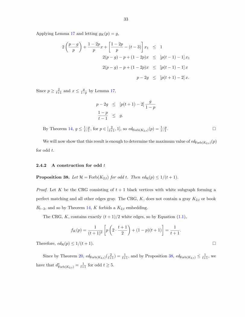
Proposition 38. Let H = Forb(K2,t) for odd t. Then edH(p) ≤ 1/(t+ 1).

Proof. Let K be the CRG consisting of t + 1 black vertices with white subgraph forming a

perfect matching and all other edges gray. The CRG, K, does not contain a gray K2,t or book

Bt−2, and so by Theorem 14, K forbids a K2,t embedding.

The CRG, K, contains exactly (t+ 1)/2 white edges, so by Equation (1.1),

fK(p) =1

(t+ 1)2

[p

(2 · t+ 1

2

)+ (1− p)(t+ 1)

]=

1

t+ 1.

Therefore, edH(p) ≤ 1/(t+ 1).

Since by Theorem 20, edForb(K2,t)(2t+1) = 1

t+1 , and by Proposition 38, edForb(K2,t) ≤1t+1 , we

have that d∗Forb(K2,t)= 1

t+1 for odd t ≥ 5.

34

2.4.3 A general lower bound for t

We conclude this section by determining a general lower bound for the edit distance function

of Forb(K2,t). It is the lower bound from Theorem 21, and it allows us to make the claim in

Theorem 22 that, in the case of odd t, there is a nondegenerate interval p∗H that achieves the

maximum value of the function.

Proof of Theorem 21. Here we use the standard bounds from Propositions 16 and 17. Let

g = gK(p), where K is a black-vertex, p-core CRG, and let NG(v) denote the gray neighborhood

of a given vertex v in K. Then if u1, . . . , u` are the vertices in the gray neighborhood, U , of a

fixed vertex of maximum weight, u0,

∑i=1

[dG(ui)− x− x (NG(ui) ∩NG(u0))] ≤ (t− 1)(1− x− dG(u0)).

The left-hand side of this inequality calculates the weight of the total gray neighborhood of

each vertex in U that must be contained in W , the set of all vertices not in U or u0. On the

right-hand side we make use of the facts that x(W ) = 1− x− dG(u0) and that no vertex in W

may be adjacent to more than (t− 1) vertices in U without violating Theorem 14 by forming

a gray K2,t with u0. Thus, applying Lemma 16,

∑i=1

[p− gp− x+

1− 2p

px(ui)

]−∑i=1

x (NG(ui) ∩NG(u0)) ≤ (t− 1)(1− x− dG(u0)).

Again considering Theorem 14 reveals that no vertex ui ∈ U can have more than t− 3 gray

neighbors in U without inducing a gray book Bt−2 with u0. Therefore,

`

[p− gp− x]

+1− 2p

pdG(u0)− (t− 3)dG(u0) ≤ (t− 1)(1− x− dG(u0))

`

[p− gp− x]≤ (t− 1)(1− x)− 1

pdG(u0).

Recalling that by Lemma 17, p−gp ≥ x, we use the pigeon-hole bound from Fact 30 ` ≥

35

dG(u0)/x to get

dG(u0)

x

[p− gp− x]≤ (t− 1)(1− x)− 1

pdG(u0)

dG(u0)

[p− gp− x]≤ (t− 1)x(1− x)− x

pdG(u0)

dG(u0)

[p− gp

+1− pp

x

]≤ (t− 1)x(1− x).

By Lemma 16, [p− gp

+1− 2p

px

] [p− gp

+1− pp

x

]≤ (t− 1)x(1− x).

Collecting terms yields,(p− gp

)2

+

[(p− gp

)(2− 3p

p

)− (t− 1)

]x+

[(1− 2p

p

)(1− pp

)+ (t− 1)

]x2 ≤ 0,

and so minimizing the left-hand side of the inequality with respect to x, we have

(p− gp

)2

−

[(t− 1)−

(p−gp

)(2−3pp

)]24[(

1−2pp

)(1−pp

)+ (t− 1)

] ≤ 0

(p− gp

)2

(4t− 5) + 2

(p− gp

)(t− 1)

(2− 3p

p

)− (t− 1)2 ≤ 0.

Using the quadratic formula,

p− gp

≤−2(t− 1)

(2−3pp

)+

√4(t− 1)2

(2−3pp

)2+ 4(t− 1)2(4t− 5)

2(4t− 5)

p− g ≤ t− 1

4t− 5

[3p− 2 +

√(2− 3p)2 + (4t− 5)p2

]g ≥ p− t− 1

4t− 5

[3p− 2 + 2

√1− 3p+ (t+ 1)p2

].

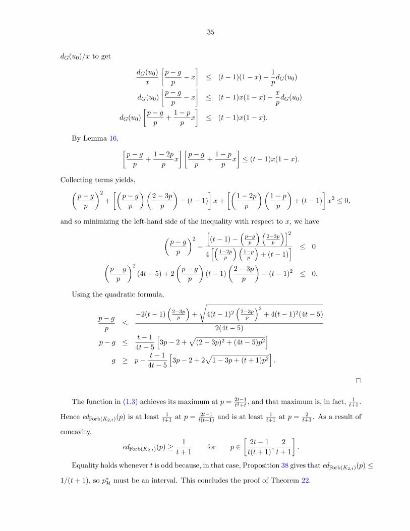
The function in (1.3) achieves its maximum at p = 2t−1t2+t

, and that maximum is, in fact, 1t+1 .

Hence edForb(K2,t)(p) is at least 1t+1 at p = 2t−1

t(t+1) and is at least 1t+1 at p = 2

t+1 . As a result of

concavity,

edForb(K2,t)(p) ≥1

t+ 1for p ∈

[2t− 1

t(t+ 1),

2

t+ 1

].

Equality holds whenever t is odd because, in that case, Proposition 38 gives that edForb(K2,t)(p) ≤

1/(t+ 1), so p∗H must be an interval. This concludes the proof of Theorem 22.

36

If t ≥ 5, then we can analyze the first and second derivatives, with respect to p, of

p(1− p)−(p− t− 1

4t− 5

[3p− 2 + 2

√1− 3p+ (t+ 1)p2

]). (2.3)

The maximum difference between p(1− p) and the lower bound in Theorem 21 on the interval

[0, 2t+1 ] is 1

t+1 and occurs when p = 2t−1t(t+1) . We can also see that (2.3) is bounded below by(

12 −

1t−1

)p(1− p).

2.5 Upper bound constructions

In this section we look at upper bound constructions for when t ≥ 5.

Subsection 2.5.1revisits the work in Section 2.3.1 on strongly regular graphs. Subsec-

tion 2.5.2 gives some constructions inspired by the analysis of triangle-free graphs in [14].

2.5.1 Results from strongly regular graph constructions

Recall that a strongly regular graph with parameters (k, d, λ, µ) is a d-regular graph on

k vertices such that each pair of adjacent vertices has λ common neighbors, and each pair

of nonadjacent vertices has µ common neighbors. Here we develop a function based on the

existence of a strongly regular graph.

Suppose that K is a CRG with all vertices black and all edges white or gray that is de-

rived from a (k, d, λ, µ)-strongly regular graph so that the edges of the strongly regular graph

correspond to gray edges of K. In such a case we recall from Section 2.3.1 that

fSk,d,λ,µ(p) =1

k+

(k − d− 2

k

)p.

As is commonly known (see [41], for instance), if a strongly regular graph with parameters

(k, d, λ, µ) exists then it is necessary, though not sufficient, for

d(d− λ− 1) = µ(k − d− 1).

If we substitute λ = t− 3 and µ = t− 1 in this equation and then solve for k, we find that

k =t− 1 + d(d+ 1)

t− 1,

37

and substituting these values into fSk,d,λ,µ(p) yields

fSk,d,λ,µ(p) =t− 1

t− 1 + d(d+ 1)+

(1− (d+ 2)(t− 1)

t− 1 + d(d+ 1)

)p.

Fixing p and minimizing fSk,d,λ,µ(p) with respect to d gives the following expression:

p(t− 2) + 2(t− 1)

4t− 5− 2(t− 1)

4t− 5

√1− 3p+ (t+ 1)p2, (2.4)

which is equal to the lower bound from (1.3) in Theorem 21.

Of course, in order to even have a chance of actually attaining (2.4) with a strongly regular

graph construction, both d and k = t−1+d(d+1)t−1 must be integers. This equation, however,

provides something of a best case scenario for strongly regular graphs, and if there is a CRG,

K, derived from a (k, d, t − 3, t − 1)-strongly regular graph that realizes equation (2.4), then

fK(p) is tangent to the lower bound in (1.3) at

p =2d+ 1

(d+ 1)(d+ 3)− t,

determining the value of edForb(K2,t)(p) exactly.

The remaining upper bounds in Theorem 27 are the result of checking constructions from

the known strongly regular graphs listed at [15]. Figure 2.2 (see Section 2.6) is a chart of the

relevant parameters and fK(p) functions for 5 ≤ t ≤ 8.

There is an additional construction defining the upper bound for t = 8 in Theorem 26,

described in the following section, and explored in more depth in Chapter 3.

2.5.2 Cycle construction

Let Crk be the cycle on k vertices raised to the rth power. Define Ck,r to be the CRG on k

black vertices with white edges corresponding to those in Crk and gray edges corresponding to

those in the complement of Crk . Let EW denotes the set of white edges for Ck,r. Then

fCk,r(p) =1

k2[(1− p)k + 2p |EW|]

=1

k2[(1− p)k + 2p(rk)]

=

(2r − 1

k

)p+

1

k.

38

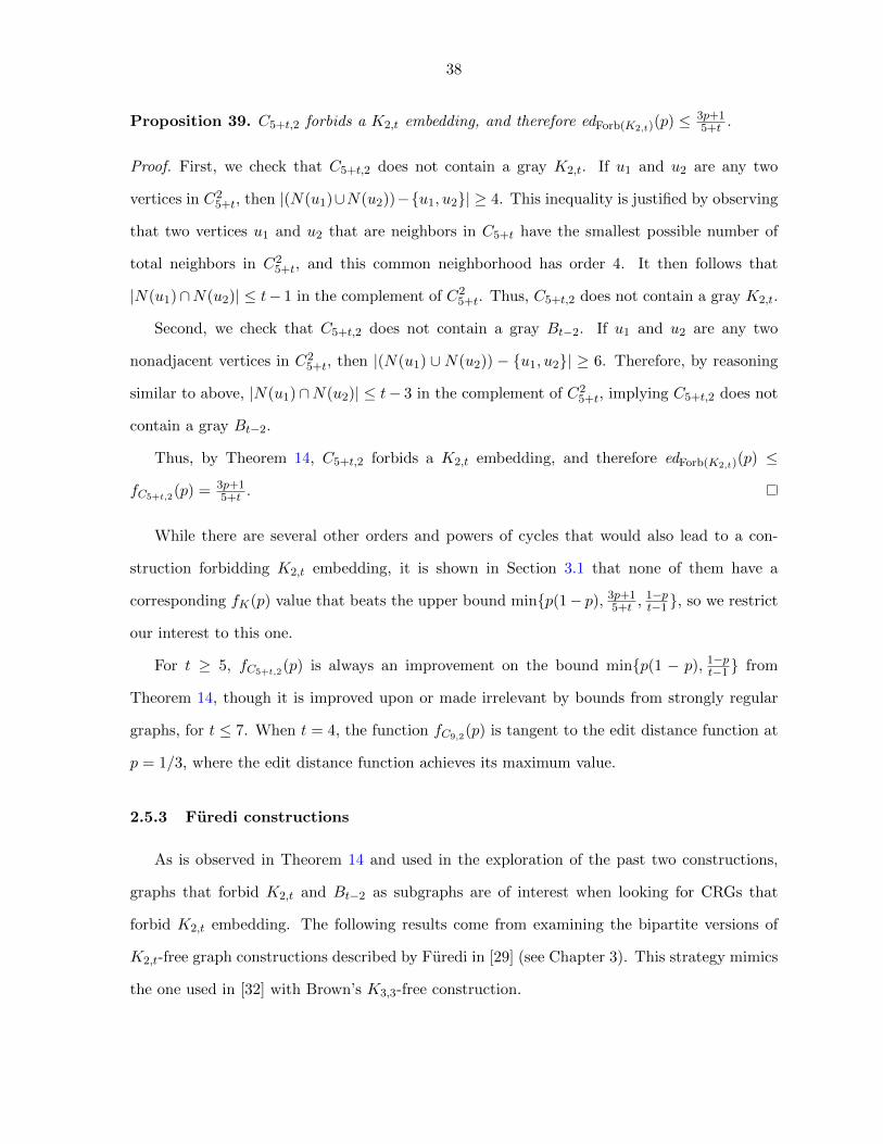
Proposition 39. C5+t,2 forbids a K2,t embedding, and therefore edForb(K2,t)(p) ≤3p+15+t .

Proof. First, we check that C5+t,2 does not contain a gray K2,t. If u1 and u2 are any two

vertices in C25+t, then |(N(u1)∪N(u2))−{u1, u2}| ≥ 4. This inequality is justified by observing

that two vertices u1 and u2 that are neighbors in C5+t have the smallest possible number of

total neighbors in C25+t, and this common neighborhood has order 4. It then follows that

|N(u1)∩N(u2)| ≤ t− 1 in the complement of C25+t. Thus, C5+t,2 does not contain a gray K2,t.

Second, we check that C5+t,2 does not contain a gray Bt−2. If u1 and u2 are any two

nonadjacent vertices in C25+t, then |(N(u1) ∪N(u2)) − {u1, u2}| ≥ 6. Therefore, by reasoning

similar to above, |N(u1)∩N(u2)| ≤ t− 3 in the complement of C25+t, implying C5+t,2 does not

contain a gray Bt−2.

Thus, by Theorem 14, C5+t,2 forbids a K2,t embedding, and therefore edForb(K2,t)(p) ≤

fC5+t,2(p) = 3p+15+t .

While there are several other orders and powers of cycles that would also lead to a con-

struction forbidding K2,t embedding, it is shown in Section 3.1 that none of them have a

corresponding fK(p) value that beats the upper bound min{p(1− p), 3p+15+t ,

1−pt−1 }, so we restrict

our interest to this one.

For t ≥ 5, fC5+t,2(p) is always an improvement on the bound min{p(1 − p), 1−pt−1 } from

Theorem 14, though it is improved upon or made irrelevant by bounds from strongly regular

graphs, for t ≤ 7. When t = 4, the function fC9,2(p) is tangent to the edit distance function at

p = 1/3, where the edit distance function achieves its maximum value.

2.5.3 Furedi constructions

As is observed in Theorem 14 and used in the exploration of the past two constructions,

graphs that forbid K2,t and Bt−2 as subgraphs are of interest when looking for CRGs that

forbid K2,t embedding. The following results come from examining the bipartite versions of

K2,t-free graph constructions described by Furedi in [29] (see Chapter 3). This strategy mimics

the one used in [32] with Brown’s K3,3-free construction.

39

Proof of Theorem 23. We take the construction described in [29] for a K2,t-free graph G on

n = (q2− 1)/(t− 1) vertices, each with degree q, where q is a prime power so that t− 1 divides

q − 1. We should note here that in the original construction from [29], loops were omitted,

reducing the degree of some vertices to q−1. It is to our advantage, however, to leave the loops

in so that the final construction will be q-regular. By the same proof as in [29], the graph with

loops still retains the property that no two vertices have a common neighborhood greater than

t− 1 even when a looped vertex is considered to be in its own neighborhood.

Next, we create a CRG, K, by taking two copies of the vertex set {v1, . . . , vn} from the

K2,t-free graph with loops described above: {v′1, . . . , v′n}, {v′′1 , . . . , v′′n}. Color all of these k = 2n

vertices black, and let EG(K) = {v′iv′′j : vivj ∈ E(G)} with all edges not in EG(K) white.

The gray subgraph of K is bipartite, so it cannot contain a Bt−2, and since no two vertices

vi and vj from the original construction have more than t− 1 common neighbors, the common

neighborhood of two vertices in the gray subgraph of K is also at most t−1. Thus by Theorem

14, K forbids a K2,t embedding.

The CRG, K, has k = 2n = 2(q2 − 1)/(t− 1) vertices and q(q2 − 1)/(t− 1) gray edges, so

by equation (1.1), fK(p) is as described in the statement of Theorem 23.

Remark 40. Though the property of being bipartite is sufficient to exclude a Bt−2 subgraph,

using a bipartite K2,t-free construction may not be the optimal choice. A more efficient CRG

may be constructed from another graph that has a gray subgraph that is both K2,t- and Bt−2-free,

but, for instance, still contains triangles.

Nevertheless, we can discover more about the potential for these constructions to improve

upon the bounds for edForb(K2,t)(p) by fixing p and considering the general formula in Theorem

23 as a continuous function with respect to q.

Lemma 41. Let t ≥ 3, and let q0 < q be prime powers such that t− 1 divides both q0 − 1 and

q − 1. If the CRG, K0, is constructed according to the proof of Theorem 23 with parameter q0

and if the CRG, K, is constructed according to the proof of Theorem 23 with parameter q, then

fK0(p) ≤ fK(p) for p ∈[

24+q0

, 13

).

40

Proof. We begin the proof by fixing p and t and analyzing φ(q) = t−1+p(2q2−q(t−1)−2t)2(q2−1) . Note

that fK0(p) = φ(q0), and fK(p) = φ(q). Consider when the derivative

φ′(q) =(t− 1)(q2p+ p+ 4qp− 2q)

2(q2 − 1)2

is positive and, therefore, φ is increasing. Since the greater value of q that makes q2p + p +

4qp − 2q = 0 (note that the leading term is nonnegative) occurs at q =(1−2p)+

√(1−2p)2−p2p , it

follows that φ′(q) ≥ 0 when q ≥ (1−2p)+√

(1−2p)2−p2p . If p < 1/3 and q0 ≥ 2(1−2p)

p , then

q > q0 ≥2(1− 2p)

p>

(1− 2p) +√

(1− 2p)2 − p2p

.

Thus, φ′(q) ≥ 0 for 24+q0

≤ p < 1/3. Therefore fK0(p) ≤ fK(p) for p in this interval.

Additionally, we can make some statements about when we can expect constructions that

originate from the K2,t-free graphs described by Furedi [29] to improve upon the bound p(1−p)

for any q.

Lemma 42. Fix t ≥ 9, and let q be a prime power such that t− 1 divides q − 1. Let K be the

CRG with parameter q described in the proof of Theorem 23, hence fK(p) = t−1+p(2q2−q(t−1)−2t)2(q2−1) .

Then for any sufficiently large prime power q and corresponding K, there is an interval of values

of p on which fK(p) < p(1 − p). Moreover as q → ∞ the left-hand endpoints of these open

intervals approach 0.

That is, we can find an infinite sequence of CRG constructions that improve upon the known

bounds for Forb(K2,t) when t ≥ 9, and the intervals on which these improvements occur get

arbitrarily close to 0.

Proof. We begin by observing that fK(p) = t−1+p(2q2−q(t−1)−2t)2(q2−1) = p − p(q(t−1)+2t−2)−(t−1)

2(q2−1) .

Thus if fK(p) < p(1− p),

p− p(q(t− 1) + 2t− 2)− (t− 1)

2(q2 − 1)< p− p2

2p2(q2 − 1) < p(q(t− 1) + 2(t− 1))− (t− 1)

2p2(q2 − 1)− p(t− 1)(q + 2) + (t− 1) < 0. (2.5)

41

The minimum value of 2p2(q2 − 1) − p(t − 1)(q + 2) + (t − 1) occurs when p = (t−1)(q+2)4(q2−1) .

Therefore, the inequality above is satisfied for some q and p values if and only if

2

[(t− 1)(q + 2)

4(q2 − 1)

]2(q2 − 1)−

[(t− 1)(q + 2)

4(q2 − 1)

](t− 1)(q + 2) + (t− 1) < 0

(t− 1)

(1− (t− 1)(q + 2)2

8(q2 − 1)

)< 0.

That is, fK(p) from the constructions in [29] is less than p(1− p) for some value of p if and

only if 1 − (t−1)(q+2)2

8(q2−1) < 0. For positive q, it is always the case that (q + 2)2 > q2 − 1, and

so any q satisfying the constraints of the original construction will improve upon the upper

bound established by p(1− p) for some p when t ≥ 9. Furthermore, for a fixed prime power q

for which t− 1 divides q − 1, it is a definite improvement for some open neighborhood around

p = (t−1)(q+2)4(q2−1) . This value approaches 0 as q → ∞, and there are an infinite number of prime

powers q such that t− 1 divides q − 1 (see [29]). Thus, it is the case that for arbitrarily small

p, we can find some q such that fK(p) < p(1− p).

Lemma 43 is an analysis of the Furedi constructions when t ≤ 8. We then show that our

bounds from these constructions do not have an effect on the value of edForb(K2,t)(p) for t ≤ 8.

Lemma 43. Fix 5 ≤ t ≤ 8, and let q be a prime power such that t−1 divides q−1. Let K be the

CRG with parameter q described in the proof of Theorem 23, hence fK(p) = t−1+p(2q2−q(t−1)−2t)2(q2−1) .

Then

q <(t− 1) +

√(t− 1)2 + (9− t)(t+ 1)

12(9− t)

. (2.6)

Proof. Returning to inequality (2.5) and performing a similar analysis to that in the proof of

Lemma 42, we see that if t ≤ 8, then 2p2(q2 − 1)− p(t− 1)(q + 2) + (t− 1) < 0 for some value

of p if and only if

(t− 1)−√

(t− 1)2 + (9− t)(t+ 1)12(9− t)

< q <(t− 1) +

√(t− 1)2 + (9− t)(t+ 1)

12(9− t)

.

The lower bound for q described above is immaterial since for t ≤ 8 it is always negative. The

upper bound completes the proof of Lemma 43.

42

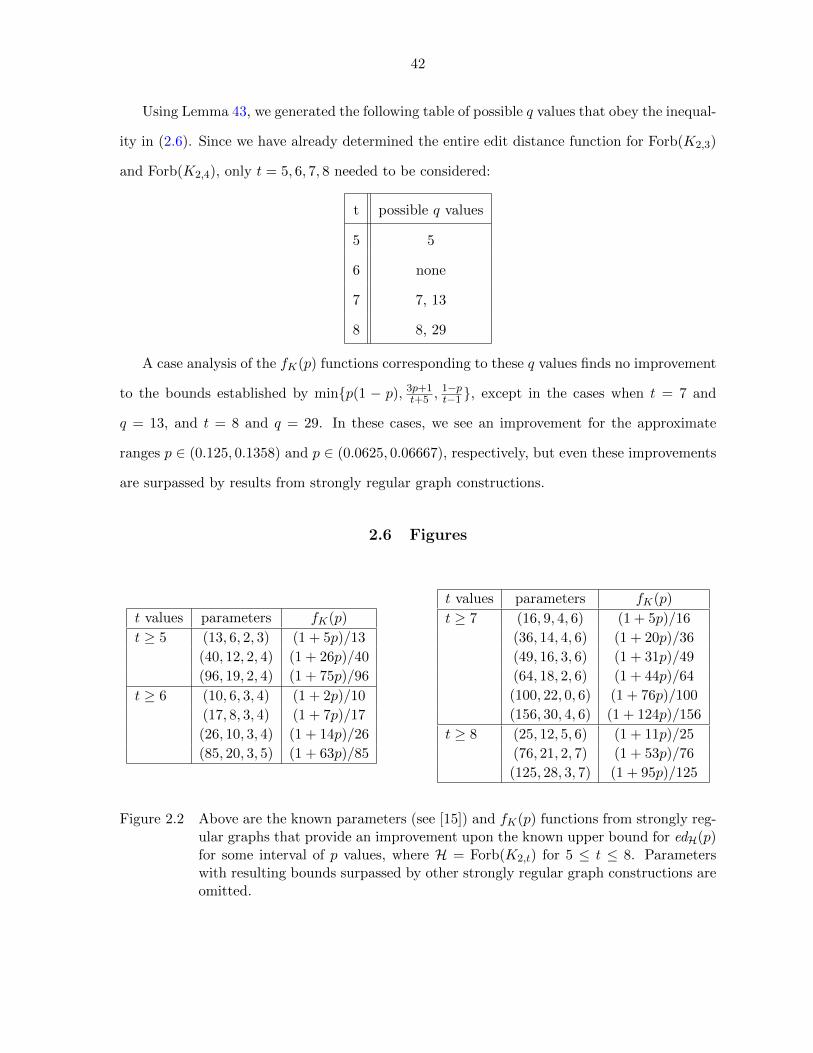
Using Lemma 43, we generated the following table of possible q values that obey the inequal-

ity in (2.6). Since we have already determined the entire edit distance function for Forb(K2,3)

and Forb(K2,4), only t = 5, 6, 7, 8 needed to be considered:

t possible q values

5 5

6 none

7 7, 13

8 8, 29

A case analysis of the fK(p) functions corresponding to these q values finds no improvement

to the bounds established by min{p(1 − p), 3p+1t+5 ,

1−pt−1 }, except in the cases when t = 7 and

q = 13, and t = 8 and q = 29. In these cases, we see an improvement for the approximate

ranges p ∈ (0.125, 0.1358) and p ∈ (0.0625, 0.06667), respectively, but even these improvements

are surpassed by results from strongly regular graph constructions.

2.6 Figures

t values parameters fK(p)

t ≥ 5 (13, 6, 2, 3) (1 + 5p)/13

(40, 12, 2, 4) (1 + 26p)/40

(96, 19, 2, 4) (1 + 75p)/96

t ≥ 6 (10, 6, 3, 4) (1 + 2p)/10

(17, 8, 3, 4) (1 + 7p)/17

(26, 10, 3, 4) (1 + 14p)/26

(85, 20, 3, 5) (1 + 63p)/85

t values parameters fK(p)

t ≥ 7 (16, 9, 4, 6) (1 + 5p)/16

(36, 14, 4, 6) (1 + 20p)/36

(49, 16, 3, 6) (1 + 31p)/49

(64, 18, 2, 6) (1 + 44p)/64

(100, 22, 0, 6) (1 + 76p)/100

(156, 30, 4, 6) (1 + 124p)/156

t ≥ 8 (25, 12, 5, 6) (1 + 11p)/25

(76, 21, 2, 7) (1 + 53p)/76

(125, 28, 3, 7) (1 + 95p)/125

Figure 2.2 Above are the known parameters (see [15]) and fK(p) functions from strongly reg-ular graphs that provide an improvement upon the known upper bound for edH(p)for some interval of p values, where H = Forb(K2,t) for 5 ≤ t ≤ 8. Parameterswith resulting bounds surpassed by other strongly regular graph constructions areomitted.

43

0.0 0.2 0.4 0.6 0.8 1.0p

0.05

0.10

0.15

0.20

0.25

gH pL

Figure 2.3 Plot of edForb(K2,3)(p) = min{p(1 − p), (1 − p)/2}. The point (p∗, d∗) = (1/2, 1/4)is indicated.

0.0 0.2 0.4 0.6 0.8 1.0p

0.05

0.10

0.15

0.20

0.25

gH pL

Figure 2.4 Plot of edForb(K2,4)(p) = min{p(1 − p), (1 + 7p)/15, (1 − p)/3}. The point(p∗, d∗) = (1/3, 2/9) is indicated.

0.0 0.1 0.2 0.3 0.4 0.5p

0.05

0.10

0.15

0.20

gH pL

Figure 2.5 Upper and lower bounds (in solid and dashed respectively) for edForb(K2,5)(p).Points indicate tangency.

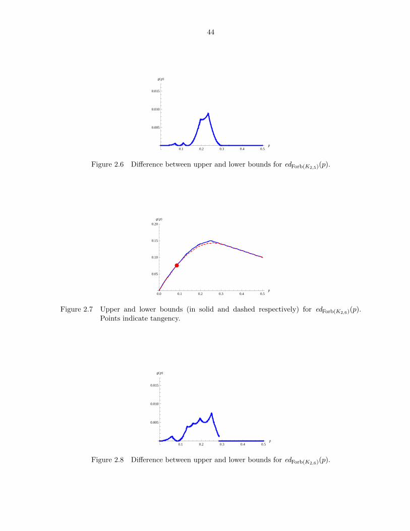
44

0.1 0.2 0.3 0.4 0.5p

0.005

0.010

0.015

gH pL

Figure 2.6 Difference between upper and lower bounds for edForb(K2,5)(p).

0.0 0.1 0.2 0.3 0.4 0.5p

0.05

0.10

0.15

0.20

gH pL

Figure 2.7 Upper and lower bounds (in solid and dashed respectively) for edForb(K2,6)(p).Points indicate tangency.

0.1 0.2 0.3 0.4 0.5p

0.005

0.010

0.015

gH pL

Figure 2.8 Difference between upper and lower bounds for edForb(K2,6)(p).

45

0.0 0.1 0.2 0.3 0.4 0.5p

0.05

0.10

0.15

0.20

gH pL

Figure 2.9 Upper and lower bounds (in solid and dashed respectively) for edForb(K2,7)(p).Points indicate tangency.

0.1 0.2 0.3 0.4 0.5p

0.005

0.010

0.015

gH pL

Figure 2.10 Difference between upper and lower bounds for edForb(K2,7)(p).

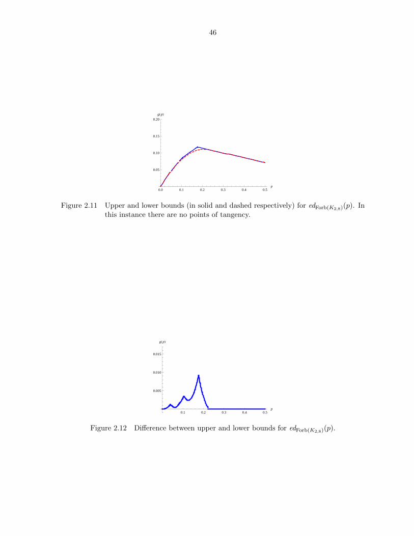
46

0.0 0.1 0.2 0.3 0.4 0.5p

0.05

0.10

0.15

0.20

gH pL

Figure 2.11 Upper and lower bounds (in solid and dashed respectively) for edForb(K2,8)(p). Inthis instance there are no points of tangency.

0.1 0.2 0.3 0.4 0.5p

0.005

0.010

0.015

gH pL

Figure 2.12 Difference between upper and lower bounds for edForb(K2,8)(p).

47

CHAPTER 3. MORE ON CYCLE POWERS AND FUREDI’S

CONSTRUCTION

3.1 General cycle constructions

As mentioned in Section 2.5.2, cycle constructions are one possible type of CRG that can

be used to provide an upper bound for the edit distance function of K2,t. Recall that if Crk is

the cycle on k vertices raised to the rth power, then Ck,r is defined to be the CRG on k black

vertices with white edges corresponding to those in Crk , and gray edges corresponding to those

in the complement of Crk . Furthermore,

fCk,r(p) =

(2r − 1

k

)p+

1

k.

In Chapter 2, the bound edForb(K2,t)(p) ≤3p+15+t is found by demonstrating that C5+t,2 forbids

a K2,t embedding. In this section, we explore what other CRG cycle constructions forbid K2,t

embedding, and demonstrate that C5+t,2 is indeed the best one for our purposes.

3.1.1 The best k for a given value of r

fCk,r(p) is monotone decreasing with respect to k. Thus, for a given r and t, the goal is to

find the largest k so that Ck,r contains neither a gray K2,t nor a gray book Bt−2 (see Theorem

14). With the goal of maximizing k with respect to this constraint in mind, it is reasonable to

assume that k ≥ 3r + 2.

Let NG(v) denote the neighborhood of v in Ck,r via gray edges and NW (v) denote the neigh-

borhood via white edges. If v1, v2 are any two vertices in Ck,r, then |NW (v1)∪NW (v2)) {v1, v2}| ≥

2r. This is because a single vertex in the white subgraph of Ck,r has 2r neighbors. The largest

common neighborhood for v1 and v2 occurs when they were neighbors in the original cycle Ck, in

48

which case |NW (v1)∪NW (v2)) {v1, v2}| = 2r. Therefore, |NG(v1)∪NG(v2)) {v1, v2}| ≤ k−2r−2.

Thus to forbid a gray K2,t, we want k − r2− 2 < t⇒ k ≤ 2r + t+ 1.

To forbid a gray Bt−2, if v1, v2 are any two vertices adjacent via a gray edge in Ck,r, then

by similar reasoning, |NG(v1) ∪NG(v2)) {v1, v2}| ≤ k − 3r − 2.

Thus, comparing these two inequalities yields that the optimal values of k for fixed r such

that Ck,r still forbids K2,t embedding are

k = 3r + t− 1 = 2 + t for r = 1

k = 2r + t+ 1 for r ≥ 2

3.1.2 Why r = 2 is optimal

From the above equations, we have that for fixed r, the optimal fCk,r(p) functions are

fC2+t,r(p) =

(1

2 + t

)p+

1

2 + tfor r = 1

fC2r+t+1,r(p) =

(2r − 1

2r + t+ 1

)p+

1

2r + t+ 1for r ≥ 2

In the case where r ≥ 2, r = 2 is always the optimal choice to minimize fC2r+t+1,r(p). One

way to see this is to observe that fC2r+t+1,r(p) is linear with respect to p and that all such lines

pass through the point p = 12+t with slopes that increase with r. What is more, these functions

only improve upon p(1− p) for p ∈ [2+t−√−8r+t2

2(1+2r+t) , 2+t+√−8r+t2

2(1+2r+t) ], and 12+t ≤

2+t−√−8r+t2

2(1+2r+t) , so the

least value of r is best. A similar type of argument also shows that r = 2 is always better than

r = 1.

Thus, fCt+5,2(p) is always optimal.

49

3.2 Furedi’s construction from [29] described

The proof of Theorem 23 alludes to the construction employed by Furedi in [29] to address

the Zarankiewicz problem for K2,t. For completeness, the construction is outlined below.

Construction 44 (Furedi [29]). The Construction of a K2,t-free graph G as described in [29]

can be accomplished as follows:

1. Find a prime power q such that t− 1 divides q − 1.

2. Let F be the finite field of order q and H be a subgroup of the multiplicative group of

F\{0} so that |H| = t− 1.

3. Divide the ordered pairs (a, b) ∈ F × F such that (a, b) 6= (0, 0) into equivalence classes

with (a, b) ∼ (a′, b′) if (a′, b′) = (ha, hb) for some h ∈ H. These equivalence classes are

the vertices of G.

4. To define the edges of G, let the vertices corresponding to the distinct equivalence classes

of (a, b) and (x, y) be adjacent if and only if ax+ by ∈ H.

By demonstrating that the system of equations

ax+ by = hα

a′x+ b′y = hβ

has at most t − 1 equivalence classes in its solution set, [29] shows that G cannot contain a

K2,t. While in [29] graphs do not contain loops, and therefore the vertices of G had degree q

if a2 + b2 /∈ H and degree q − 1 if a2 + b2 ∈ H, if we allow loops in G for vertices of degree

q − 1, then the common neighborhood of each pair of vertices is still of order at most t− 1 for

the same reason as before. Thus, we can construct a K2,t-free, q-regular bipartite graph G′ as

described in the proof of Theorem 23.

50

CHAPTER 4. CONCLUSIONS AND FUTURE DIRECTIONS

The results and methods in this thesis demonstrate how a combination of symmetrization

techniques from [33], observations from the study of 2-coloured multigraphs, and classical and

extremal graph theory constructions can be applied to learn more about the edit distance

function for the hereditary property Forb(K2,t).

While Forb(K2,t) is only on of many types of hereditary properties for which this function

is unknown, the results in this specific case are interesting for several reasons.

First, the connection between our lower bound in Theorem 21 and upper bounds from

(k, d, t−3, t−1)-strongly regular graphs begs the question of not only what advances in knowl-

edge of strongly regular graphs can do to help determine the edit distance function for these

hereditary properties, but also whether more knowledge of the edit distance for these prop-

erties could lend some insight into the existence of these types of graphs. To the best of my

knowledge, it is unknown whether there is a finite or infinite number of strongly regular graphs

of this form [19].

Second, the emerging impact of Furedi’s constructions for large t leads to the question of

what is happening to the optimal p-core CRG constructions for small p as t gets large?

Third, what is the significance of entire intervals of p∗ values corresponding to the maximum

of the edit distance function for odd t, and when can we expect these intervals in general?

There are also still a number of other open questions and avenues for future work in this

area. For instance, questions of stability: how many different p-core colored regularity graphs

witness the exact value of this or other hereditary properties for a fixed p and H? One way

to view these p-core constructions is as a template for an optimal way to edit the edges of the

random graph G(n, p) to make it a member of a hereditary property. Therefore, it is natural

to ask questions about how many such templates exist.

51

Another avenue for future work is to answer the question of what can be said about analo-

gous functions for graph metrics other than edit distance? Can we define a similar such function

using these metrics, and if so, will it be continuous and/or concave?

52

BIBLIOGRAPHY

[1] Alekseev, V. E. (1992). Range of values of entropy of hereditary classes of graphs. Diskret.

Mat., 4(2):148–157.

[2] Alon, N., Fischer, E., Krivelevich, M., and Szegedy, M. (2000). Efficient testing of large

graphs. Combinatorica, 20(4):451–476.

[3] Alon, N. and Shapira, A. (2008). A characterization of the (natural) graph properties

testable with one-sided error. SIAM J. Comput., 37(6):1703–1727.

[4] Alon, N. and Stav, U. (2008a). The maximum edit distance from hereditary graph proper-

ties. J. Combin. Theory Ser. B, 98(4):672–697.

[5] Alon, N. and Stav, U. (2008b). What is the furthest graph from a hereditary property?

Random Structures Algorithms, 33(1):87–104.

[6] Alon, N. and Stav, U. (2009). Stability-type results for hereditary properties. J. Graph

Theory, 62(1):65–83.

[7] Axenovich, M., Kezdy, A., and Martin, R. (2008). On the editing distance of graphs. J.

Graph Theory, 58(2):123–138.

[8] Axenovich, M. and Martin, R. (2006). Avoiding patterns in matrices via a small number of

changes. SIAM J. Discrete Math., 20(1):49–54 (electronic).

[9] Balogh, J. and Martin, R. (2008). Edit distance and its computation. Electron. J. Combin.,

15(1):Research Paper 20, 27.

[10] Bollobas, B. (2001). Random graphs, volume 73 of Cambridge Studies in Advanced Math-

ematics. Cambridge University Press, Cambridge, second edition.

53

[11] Bollobas, B. and Thomason, A. (1995). Projections of bodies and hereditary properties of

hypergraphs. Bull. London Math. Soc., 27(5):417–424.

[12] Bollobas, B. and Thomason, A. (1997). Hereditary and monotone properties of graphs. In

The mathematics of Paul Erdos, II, volume 14 of Algorithms Combin., pages 70–78. Springer,

Berlin.

[13] Bollobas, B. and Thomason, A. (2000). The structure of hereditary properties and colour-

ings of random graphs. Combinatorica, 20(2):173–202.

[14] Brandt, S. (1999). On the structure of dense triangle-free graphs. Combin. Probab. Com-

put., 8(3):237–245.

[15] Brouwer, A. E. Parameters of strongly regular graphs. http://www.win.tue.nl/~aeb/

graphs/srg/srgtab.html (accessed July 1, 2010).

[16] Brown, W. G. (1966). On graphs that do not contain a Thomsen graph. Canad. Math.

Bull., 9:281–285.

[17] Chen, D., Eulenstein, O., Fernandez-Baca, D., and Sanderson, M. (2002). Supertrees by

flipping. In Computing and combinatorics, volume 2387 of Lecture Notes in Comput. Sci.,

pages 391–400. Springer, Berlin.

[18] Chen, G., Faudree, R. J., and Gould, R. J. (2008). Saturation numbers of books. Electron.

J. Combin., 15(1):Research Paper 118, 12.

[19] Elzinga, R. J. (2003). Strongly regular graphs: values of λ and µ for which there are only

finitely many feasible (v, k, λ, µ). Electron. J. Linear Algebra, 10:232–239 (electronic).

[20] Erdos, P. (1964/1965). On an extremal problem in graph theory. Colloq. Math., 13:251–

254.

[21] Erdos, P., Faudree, R., Pach, J., and Spencer, J. (1988). How to make a graph bipartite.

J. Combin. Theory Ser. B, 45(1):86–98.

54

[22] Erdos, P., Furedi, Z., Rothschild, B. L., and Sos, V. T. (1999). Induced subgraphs of given

sizes. Discrete Math., 200(1-3):61–77. Paul Erdos memorial collection.

[23] Erdos, P., Gyarfas, A., and Ruszinko, M. (1998). How to decrease the diameter of triangle-

free graphs. Combinatorica, 18(4):493–501.

[24] Erdos, P., Gyori, E., and Simonovits, M. (1992). How many edges should be deleted

to make a triangle-free graph bipartite? In Sets, graphs and numbers (Budapest, 1991),

volume 60 of Colloq. Math. Soc. Janos Bolyai, pages 239–263. North-Holland, Amsterdam.

[25] Erdos, P. and Renyi, A. (1959). On random graphs. I. Publ. Math. Debrecen, 6:290–297.

[26] Erdos, P. and Simonovits, M. (1966). A limit theorem in graph theory. Studia Sci. Math.

Hungar, 1:51–57.

[27] Erdos, P. and Stone, A. H. (1946). On the structure of linear graphs. volume 52, pages

1087–1091.

[28] Furedi, Z. (1991). Turan type problems. In Surveys in combinatorics, 1991 (Guildford,

1991), volume 166 of London Math. Soc. Lecture Note Ser., pages 253–300. Cambridge Univ.

Press, Cambridge.

[29] Furedi, Z. (1996). New asymptotics for bipartite Turan numbers. J. Combin. Theory Ser.

A, 75(1):141–144.

[30] Janson, S., Luczak, T., and Rucinski, A. (2000). Random graphs. Wiley-Interscience Series

in Discrete Mathematics and Optimization. Wiley-Interscience, New York.

[31] Komlos, J. and Simonovits, M. (1996). Szemeredi’s regularity lemma and its applications

in graph theory. In Combinatorics, Paul Erdos is eighty, Vol. 2 (Keszthely, 1993), volume 2

of Bolyai Soc. Math. Stud., pages 295–352. Janos Bolyai Math. Soc., Budapest.

[32] Marchant, E. and Thomason, A. (2010). Extremal graphs and multigraphs with two

weighted colours. In Fete of combinatorics and computer science, volume 20 of Bolyai Soc.

Math. Stud., pages 239–286. Janos Bolyai Math. Soc., Budapest.

55

[33] Martin, R. The edit distance function and symmetrization. arXiv:1007.1897v3.

[34] Martin, R. and McKay, T. On the edit distance from K 2,t-free graphs. Submitted.

[35] Promel, H. J. and Steger, A. (1991). Excluding induced subgraphs: quadrilaterals. Random

Structures Algorithms, 2(1):55–71.

[36] Promel, H. J. and Steger, A. (1992). Excluding induced subgraphs. III. A general asymp-

totic. Random Structures Algorithms, 3(1):19–31.

[37] Promel, H. J. and Steger, A. (1993). Excluding induced subgraphs. II. Extremal graphs.

Discrete Appl. Math., 44(1-3):283–294.

[38] Scheinerman, E. R. and Zito, J. (1994). On the size of hereditary classes of graphs. J.

Combin. Theory Ser. B, 61(1):16–39.

[39] Szemeredi, E. (1978). Regular partitions of graphs. In Problemes combinatoires et theorie

des graphes (Colloq. Internat. CNRS, Univ. Orsay, Orsay, 1976), volume 260 of Colloq.

Internat. CNRS, pages 399–401. CNRS, Paris.

[40] Thomason, A. Graphs, colours, weights and hereditary properties. Preprint.

[41] West, D. B. (2001). Introduction to Graph Theory. Prentice Hall, Upper Saddle River,

NJ, 2nd edition.