The Effect of Modelling Parameters on the

Value of GMWB Guarantees

Z. Chen∗, K. Vetzal† P.A. Forsyth‡

December 17, 2007

Abstract

In this article, an extensive study of the no-arbitrage fee for Guaranteed Minimum With-drawal Benefit (GMWB) variable annuity riders is carried out. Taking into account such con-tractual features as the separation of mutual fund fees and the fees earmarked for hedging theguarantee, as well as the possibility of jumps in the value of the underlying asset, increases thevalue of the GMWB guarantee considerably. We also explore the effects of various modellingassumptions on the optimal withdrawal strategy of the contract holder, as well as the impacton the guarantee value of sub-optimal withdrawal behaviour. Our general conclusions are thatonly if several unrealistic modelling assumptions are made is it possible to obtain GMWB feesin the same range as is normally charged. In all other cases, it would appear that typical feesare not enough to cover the cost of hedging these guarantees.

Keywords: Variable annuities, pensions, GMWB guarantees

Insurance Branch Code: IM10;IE43;IB13

JEL Classification: G22

1 Introduction

Throughout the developed world, both companies and governments are moving away from definedbenefit pension plans to defined contribution (DC) plans. Under a DC plan, the holder has controlof the accumulated pension assets, but assumes the risk of investing these assets. Most DC holdershave no choice but to invest in risky assets in order to provide sufficient income during theirretirement years.

As pointed out in Milevsky and Salisbury (2006), before retiring, the DC plan holder is exposedto market risks, but the order of random returns is immaterial. However, once the DC plan holderretires, and begins to withdraw funds from the plan, the holder is also exposed to the risk from the

∗David R. Cheriton School of Computer Science, University of Waterloo, Waterloo ON, Canada N2L 3G1 e-mail:

z4chen@uwaterloo.ca†School of Accounting and Finance, University of Waterloo, Waterloo ON, Canada N2L 3G1

kvetzal@uwaterloo.ca‡David R. Cheriton School of Computer Science, University of Waterloo, Waterloo ON, Canada N2L 3G1

paforsyt@uwaterloo.ca

1

order of the returns. Losses in the early years of retirement can be devastating, and can result ina rapid exhaustion of the plan.

In order to the manage the risk associated with the random order of returns after the DC holderretires and begins to withdraw funds from the plan, many insurance companies are offering variableannuities with a Guaranteed Minimum Withdrawal Benefit (GMWB) rider.

A GMWB contract involves an initial lump sum payment to an insurance company. These fundsare then invested in risky assets, typically a mutual fund. The policy holder is then entitled towithdraw funds (usually annually or semi-annually) at a contractually specified rate. The GMWBpromises to return at least the entire original investment, regardless of the performance of theunderlying risky investment. The policy holder may withdraw at a higher or lower rate than thecontract rate (or even to surrender instantaneously) subject to certain penalties and conditions.

In this article, we will value the GMWB contract from a financial no-arbitrage point of view.Previous work on GMWBs following this approach includes Milevsky and Salisbury (2006), Daiet al. (2007), and Bauer et al. (2006). In Milevsky and Salisbury (2006) and Dai et al. (2007), anidealized contract is studied and valued using optimal stochastic control techniques. More generalcontracts are considered in Bauer et al. (2006). All of these authors agree that GMWB guaranteesappear to be underpriced in the market. In other words, insurance companies do not appear tobe collecting enough in the way of fees to cover all of the costs associated with hedging theseguarantees.

The objective of this paper is to examine in some detail some generalizations of the idealizedcontract discussed in Dai et al. (2007). We will determine the effect of various parameters andassumptions on the fair fee associated with the guarantee. In particular, we study the following:

• In practice, the underlying mutual fund charges a separate layer of fees for managing the fund.It has been suggested that the apparent underfunding of the GMWB rider can be explainedif we assume that some of these mutual fund fees are diverted to managing the GMWB rider.However, our experience in pricing other pension plan guarantees (Windcliff et al., 2001, 2002;Le Roux, 2000) suggests that the mutual fund fees are not available for hedging purposes.We will derive the no-arbitrage partial differential equation (PDE) which results from thisfee splitting, and provide numerical results which show the effect of the fee splitting. Thisfee separation is important in practice, and does not appear to have been taken into accountin previous work (e.g. Milevsky and Salisbury, 2006; Dai et al., 2007; Bauer et al., 2006).Inclusion of this fee separation increases the value of the GMWB rider.

• Cramer et al. (2007) discuss various assumptions about investor behavior when pricing vari-able annuities. A conservative approach is to assume optimal investor behavior, and then torecognize extraordinary earnings in the event of sub-optimal behavior. Another possibility isto develop a model of non-optimal behavior, and incorporate this into the pricing model. Wewill examine both approaches in this paper. Our base case assumes optimal behaviour, butwe also model the effect of sub-optimal withdrawal behavior using the approach suggested inHo et al. (2005). Sub-optimal behavior considerably reduces the value of the GMWB rider.

• We will include results with both the classic Geometric Brownian motion process for theunderlying asset, as well as a jump diffusion process, which may be a more realistic modelfor long term guarantees. Making the assumption that there is reasonable (risk neutral)probability of a market crash during the lifetime of the guarantee dramatically increases thevalue of the GMWB rider.

2

• We will also examine the effect of various contract parameters, such as reset provisions,maturities, withdrawal intervals, and surrender charges. Some contract features (e.g. the resetprovision) have almost no effect on the value of the guarantee, while others have considerableinfluence. In addition to the value of the guarantee, we explore the impact of some of thesevarious alternative modelling assumptions on the policyholder’s optimal withdrawal strategy.Plots of the contour levels of the optimal withdrawal amounts show that the investor’s optimalstrategy can be quite sensitive to modelling assumptions.

2 Contract Description

We briefly review the GMWB rider contract description. For more details, we refer the readerto Milevsky and Salisbury (2006) and Dai et al. (2007). The contract consists of a personal sub-account invested in a risky asset, as well as a guarantee account. At the inception of the contract,the holder pays a lump sum to the insurer, which forms the initial balance of the sub-account andthe guarantee account. The policy holder pays a fee proportional to the sub-account balance.

The GMWB rider allows the holder to withdraw funds on an annual or semi-annual basis. Eachwithdrawal reduces the amount in the guarantee account and the sub-account on a dollar for dollarbasis. The holder can continue to withdraw as long as the guarantee account is above zero, even ifthe sub-account balance is zero. At the maturity of the contract, the holder receives the maximumof the sub-account balance or the guarantee account balance, net of any fees.

Note that this represents an idealized GMWB rider, and there are many variations of this basiccontract.

3 Formulation

We assume that the withdrawal occurs only at predetermined discrete times. This problem canalso be posed in terms of continuous withdrawals (Chen and Forsyth, 2007). However, as we shallverify in some numerical tests, the value of the continuous withdrawal formulation is very close tothe discrete withdrawal case if the withdrawal intervals are less than one year. In addition, manycontracts only allow discrete withdrawals.

Similar to the work in Milevsky and Salisbury (2006) and Dai et al. (2007), we will ignoremortality effects in the following. We plan to study the effect of mortality contract features infuture work.

Let W denote the balance of the personal variable annuity sub-account. Recall that W isinvested in a risky asset. Let A denote the current balance of the guarantee account. Let W0 bethe initial sub-account balance and guarantee account balance which is the same as the premiumpaid upfront. Then A can have any value lying in [0,W0]. Let αtot ≥ 0 denote the proportionaltotal fees (including mutual fund management expenses and fees charged for the GMWB rider)paid by the policy holder. Let αg be the fee paid to fund the guarantee, and αm be the mutualfund management fee, so that αtot = αg + αm.

We assume that the risk neutral process of the sub-account value W is modeled by a stochasticdifferential equation (SDE) given by

dW = (r − αtot)Wdt + σWdZ + dA, if W > 0 (1)dW = 0, if W = 0. (2)

3

Year Surrender Charge κ

0 ≤ t < 2 8%2 ≤ t < 3 7%3 ≤ t < 4 6%4 ≤ t < 5 5%5 ≤ t < 6 4%6 ≤ t < 7 3%

t ≥ 7 0%

Table 1: Time-dependent surrender charges κ(t).

Let τ = T − t, where T is the expiry date of the contract. Let τk, k = 0, . . . ,K − 1 be the kthwithdrawal time going backwards in time with τ0 = 0 and τK = T . There is no withdrawal allowedat τK = T (the inception of the contract). We denote by γk the control variable representing thediscrete withdrawal amount at τ = τk; γk can take any value in γk ∈ [0, A].

Let Gk represent the contract withdrawal amount at τk. If γk ≤ Gk, no penalty is imposed.However, if γk > Gk, then there is a proportional penalty charge κ(γk−Gk), that is, the net amountreceived by the policyholder is γk−κ(γk−Gk) if γk > Gk, where κ is a positive constant representingthe deferred surrender charge. We assume that the penalty (surrender) fees are available to fundthe GMWB guarantee.

Consequently, the cash-flow received by the policyholder at the discrete withdrawal time τ = τk

as a function of γk, denoted by f(γk), is given by

f(γk) =

{γk if 0 ≤ γk ≤ Gk

γk − κ(γk −Gk) if γk > Gk. (3)

In a typical contract, the deferred surrender charge κ = κ(t) is time-dependent and normallydecreases over time to zero. Table 1 shows a typical specification for κ(t).

Let V (W,A, τ) denote the total value of the variable annuity including the GMWB guaranteeas a function of (W,A, τ). Note that V includes all the cash flows to the policy holder, not just theGMWB guarantee cash flows.

In Appendix A, we derive the equations which determine the no-arbitrage value of V . As inDai et al. (2007), the terminal condition for the annuity is

V (W,A, τ = 0) = max(W,A(1− κ)). (4)

At the withdrawal time τ = τk, V satisfies the following optimality condition

V (W,A, τk+) = supγk∈[0,A]

[V

(max(W − γk, 0), A− γk, τk

)+ f(γk)

], k = 0, . . . ,K − 1, (5)

where τk+ denotes the time infinitesimally after τk (recall from the definition of τ that time isrunning backwards). Equation (5) has the intuitive interpretation that the policyholder will selectthe withdrawal which maximizes the total value of the cash flow received and the future value ofthe annuity after withdrawal.

4

Parameter ValueT Expiry time 10 yearsr Interest rate 5%G Contract withdrawal amount 10W0 Initial lump-sum premium 100σ Volatility .15

∆τk Withdrawal interval 1 yearαm Mutual fund fee 1%

Table 2: Base case parameters.

Within each time interval [τk+, τk+1], k = 0, . . . ,K − 1, the annuity value function V (W,A, τ),solves the following linear PDE (see Appendix A) which has A dependence only through equation(5):

Vτ = LV + αmW, τ ∈ [τk+, τk+1], k = 0, . . . ,K − 1. (6)

where the operator L is

LV =12σ2W 2VWW + (r − αtot)WVW − rV. (7)

The no-arbitrage insurance fee αg (recall αtot = αg + αm) is determined so that the contractvalue V at τ = T is equal to the initial premium W0 paid by the investor (Milevsky and Salisbury,2006; Dai et al., 2007; Cramer et al., 2007). The equations (4-7) are solved numerically using themethods described in Chen and Forsyth (2007). In the following, all results are given correct tothe number of digits shown, based on grid and timestep refinement studies.

4 Numerical Results

4.1 Base Case

We first compute the value of the guarantee for a representative base case, and then perturb theproblem parameters and compare to this base case. The base case parameters are given in Table 2,with the surrender charge κ(t) (see equation (3)) given in Table 1.

For this base case, the no-arbitrage insurance fee is αg = 117 basis points. Figure 1 shows acontour plot of the optimal withdrawal strategy γk at the first withdrawal time (t = 1) for differentvalues of W and A. In particular, we show contour levels of γ = 10, γ = .2. We choose these twocontour levels to show that in some cases the optimal withdrawal amount γ rapidly changes fromthe contract amount Gk to zero. (Due to contouring artifacts, a contour value γ < .2 results invery jagged contour levels, since it is difficult to determine numerically the zero withdrawal region).For practical purposes, the γ = .2 contour level shows the region where it is optimal to withdrawnothing. For a discussion of the conditions under which it may be optimal to withdraw nothing,see Chen and Forsyth (2007).

From Figure 1, we can observe the following:

• There is a shaded region in the left side of the figure representing excessive withdrawals (i.e.withdrawals above the contract amount) when A dominates W . In this region, it is unlikely

5

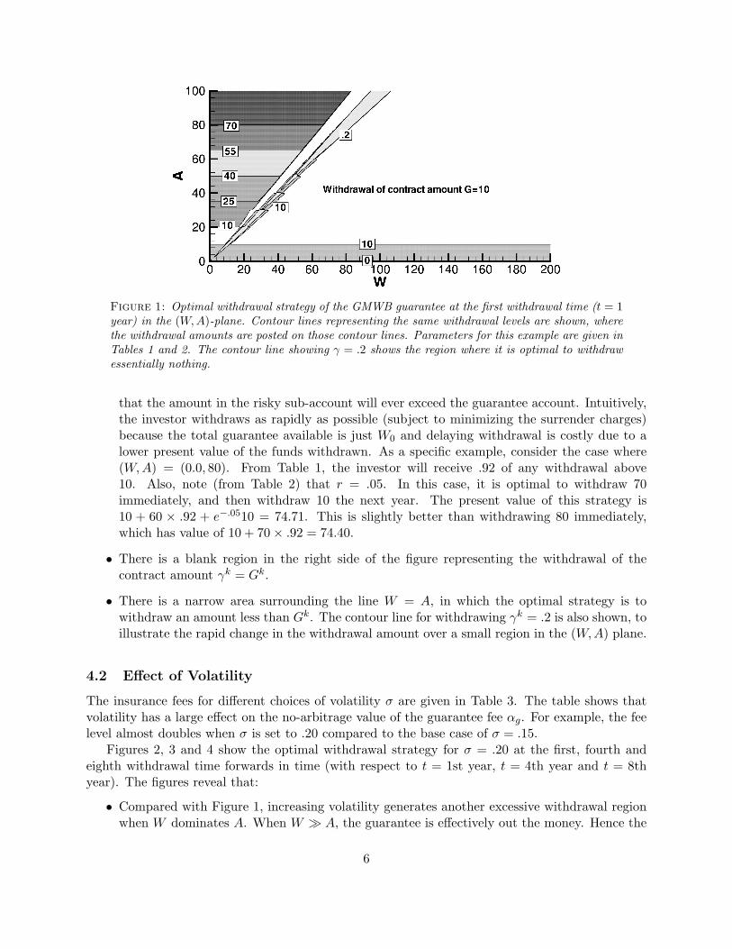
Figure 1: Optimal withdrawal strategy of the GMWB guarantee at the first withdrawal time (t = 1year) in the (W,A)-plane. Contour lines representing the same withdrawal levels are shown, wherethe withdrawal amounts are posted on those contour lines. Parameters for this example are given inTables 1 and 2. The contour line showing γ = .2 shows the region where it is optimal to withdrawessentially nothing.

that the amount in the risky sub-account will ever exceed the guarantee account. Intuitively,the investor withdraws as rapidly as possible (subject to minimizing the surrender charges)because the total guarantee available is just W0 and delaying withdrawal is costly due to alower present value of the funds withdrawn. As a specific example, consider the case where(W,A) = (0.0, 80). From Table 1, the investor will receive .92 of any withdrawal above10. Also, note (from Table 2) that r = .05. In this case, it is optimal to withdraw 70immediately, and then withdraw 10 the next year. The present value of this strategy is10 + 60 × .92 + e−.0510 = 74.71. This is slightly better than withdrawing 80 immediately,which has value of 10 + 70× .92 = 74.40.

• There is a blank region in the right side of the figure representing the withdrawal of thecontract amount γk = Gk.

• There is a narrow area surrounding the line W = A, in which the optimal strategy is towithdraw an amount less than Gk. The contour line for withdrawing γk = .2 is also shown, toillustrate the rapid change in the withdrawal amount over a small region in the (W,A) plane.

4.2 Effect of Volatility

The insurance fees for different choices of volatility σ are given in Table 3. The table shows thatvolatility has a large effect on the no-arbitrage value of the guarantee fee αg. For example, the feelevel almost doubles when σ is set to .20 compared to the base case of σ = .15.

Figures 2, 3 and 4 show the optimal withdrawal strategy for σ = .20 at the first, fourth andeighth withdrawal time forwards in time (with respect to t = 1st year, t = 4th year and t = 8thyear). The figures reveal that:

• Compared with Figure 1, increasing volatility generates another excessive withdrawal regionwhen W dominates A. When W � A, the guarantee is effectively out the money. Hence the

6

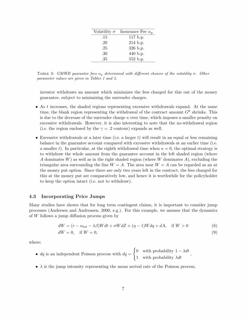
Volatility σ Insurance Fee αg

.15 117 b.p.

.20 214 b.p.

.25 326 b.p.

.30 440 b.p.

.35 552 b.p.

Table 3: GMWB guarantee fees αg determined with different choices of the volatility σ. Otherparameter values are given in Tables 1 and 2.

investor withdraws an amount which minimizes the fees charged for this out of the moneyguarantee, subject to minimizing the surrender charges.

• As t increases, the shaded regions representing excessive withdrawals expand. At the sametime, the blank region representing the withdrawal of the contract amount Gk shrinks. Thisis due to the decrease of the surrender charge κ over time, which imposes a smaller penalty onexcessive withdrawals. However, it is also interesting to note that the no-withdrawal region(i.e. the region enclosed by the γ = .2 contour) expands as well.

• Excessive withdrawals at a later time (i.e. a larger t) will result in an equal or less remainingbalance in the guarantee account compared with excessive withdrawals at an earlier time (i.e.a smaller t). In particular, at the eighth withdrawal time when κ = 0, the optimal strategy isto withdraw the whole amount from the guarantee account in the left shaded region (whereA dominates W ) as well as in the right shaded region (where W dominates A), excluding thetriangular area surrounding the line W = A. The area near W = A can be regarded as an atthe money put option. Since there are only two years left in the contract, the fees charged forthis at the money put are comparatively low, and hence it is worthwhile for the policyholderto keep the option intact (i.e. not to withdraw).

4.3 Incorporating Price Jumps

Many studies have shown that for long term contingent claims, it is important to consider jumpprocesses (Andersen and Andreasen, 2000, e.g.). For this example, we assume that the dynamicsof W follows a jump diffusion process given by

dW = (r − αtot − λβ)Wdt + σWdZ + (η − 1)Wdq + dA, if W > 0 (8)dW = 0, if W = 0, (9)

where:

• dq is an independent Poisson process with dq =

{0 with probability 1− λdt

1 with probability λdt,

• λ is the jump intensity representing the mean arrival rate of the Poisson process,

7

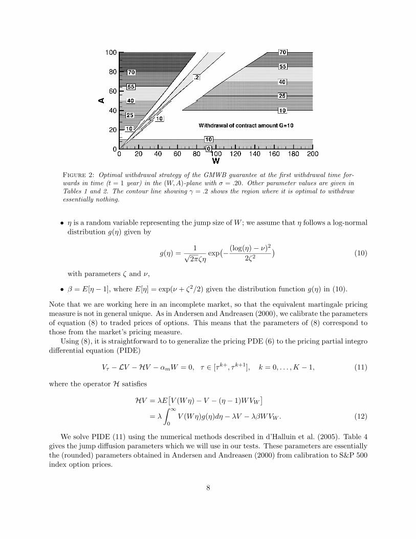
Figure 2: Optimal withdrawal strategy of the GMWB guarantee at the first withdrawal time for-wards in time (t = 1 year) in the (W,A)-plane with σ = .20. Other parameter values are given inTables 1 and 2. The contour line showing γ = .2 shows the region where it is optimal to withdrawessentially nothing.

• η is a random variable representing the jump size of W ; we assume that η follows a log-normaldistribution g(η) given by

g(η) =1√

2πζηexp

(−(log(η)− ν)2

2ζ2

)(10)

with parameters ζ and ν,

• β = E[η − 1], where E[η] = exp(ν + ζ2/2) given the distribution function g(η) in (10).

Note that we are working here in an incomplete market, so that the equivalent martingale pricingmeasure is not in general unique. As in Andersen and Andreasen (2000), we calibrate the parametersof equation (8) to traded prices of options. This means that the parameters of (8) correspond tothose from the market’s pricing measure.

Using (8), it is straightforward to to generalize the pricing PDE (6) to the pricing partial integrodifferential equation (PIDE)

Vτ − LV −HV − αmW = 0, τ ∈ [τk+, τk+1], k = 0, . . . ,K − 1, (11)

where the operator H satisfies

HV = λE[V (Wη)− V − (η − 1)WVW

]= λ

∫ ∞

0V (Wη)g(η)dη − λV − λβWVW . (12)

We solve PIDE (11) using the numerical methods described in d’Halluin et al. (2005). Table 4gives the jump diffusion parameters which we will use in our tests. These parameters are essentiallythe (rounded) parameters obtained in Andersen and Andreasen (2000) from calibration to S&P 500index option prices.

8

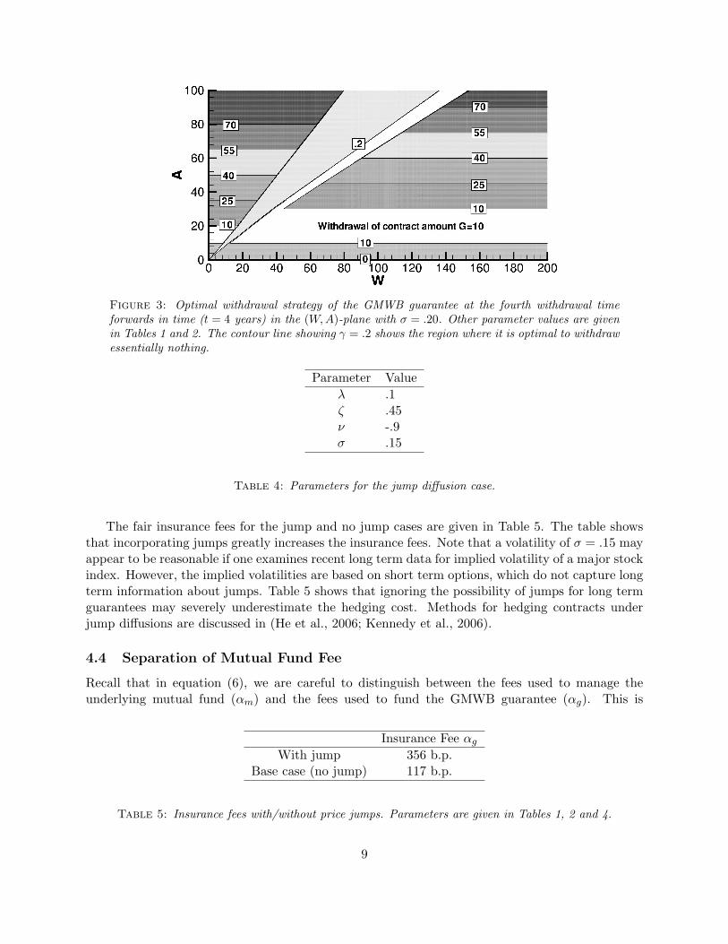
Figure 3: Optimal withdrawal strategy of the GMWB guarantee at the fourth withdrawal timeforwards in time (t = 4 years) in the (W,A)-plane with σ = .20. Other parameter values are givenin Tables 1 and 2. The contour line showing γ = .2 shows the region where it is optimal to withdrawessentially nothing.

Parameter Valueλ .1ζ .45ν -.9σ .15

Table 4: Parameters for the jump diffusion case.

The fair insurance fees for the jump and no jump cases are given in Table 5. The table showsthat incorporating jumps greatly increases the insurance fees. Note that a volatility of σ = .15 mayappear to be reasonable if one examines recent long term data for implied volatility of a major stockindex. However, the implied volatilities are based on short term options, which do not capture longterm information about jumps. Table 5 shows that ignoring the possibility of jumps for long termguarantees may severely underestimate the hedging cost. Methods for hedging contracts underjump diffusions are discussed in (He et al., 2006; Kennedy et al., 2006).

4.4 Separation of Mutual Fund Fee

Recall that in equation (6), we are careful to distinguish between the fees used to manage theunderlying mutual fund (αm) and the fees used to fund the GMWB guarantee (αg). This is

Insurance Fee αg

With jump 356 b.p.Base case (no jump) 117 b.p.

Table 5: Insurance fees with/without price jumps. Parameters are given in Tables 1, 2 and 4.

9

Figure 4: Optimal withdrawal strategy of the GMWB guarantee at the eighth withdrawal timeforwards in time (t = 8 years) in the (W,A)-plane with σ = .20. Other parameter values are givenin Tables 1 and 2. The contour line showing γ = .2 shows the region where it is optimal to withdrawessentially nothing.

Mutual Fund Fee αm Insurance Fee αg

0.0% 88 b.p.0.5% 102 b.p.1.0% 117 b.p.1.5% 136 b.p.2.0% 157 b.p.2.5% 184 b.p.

Table 6: Insurance fees determined by different choices of the mutual fund fees. Other parametervalues are given in Tables 1 and 2.

because the provider of the GWMB rider may be a completely separate business unit from the unitmanaging the mutual fund (Le Roux, 2000). A precise hedging scenario for this case is given inAppendix A.

The no-arbitrage GMWB guarantee fees αg for different choices of the mutual fund fees αm

(assuming no jumps in W ) are given in Table 6. The table shows that the GMWB fee αg is verysensitive to the mutual fund fee αm. The effect of the mutual fund fee on the GMWB fee hasnot been taken into account previously. Note that a mutual fund fee of αm = 1.0% increases theGMWB fee by 29 b.p. compared to the case where αm = 0. The intuition for this is straightforward:the guarantee applies to the initial value of the account W0, prior to any fees being deducted. Asthe mutual fund fees increase, the account value is correspondingly reduced over time, therebyincreasing the value of the guarantee.

4.5 Constant Surrender Charge

Table 7 provides the GMWB guarantee fees for a constant surrender charge κ = 8% and for thebase case κ(t) as in Table 1. It is perhaps surprising that the GMWB fee does not appear to

10

Insurance Fee αg

Constant κ 95 b.p.Decreasing κ 117 b.p.

Table 7: Insurance fees for constant/decreasing κ. For the decreasing κ(t) case, the data is givenin Table 1. For the constant κ case, the flat rate is 8%. Other parameter values are in Table 2.

decrease greatly for the case where the surrender fee is constant compared to the case where κ(t)decreases to zero. Intuitively, one reason for this is because the reported values are at t = 0, andthe benefit to the investor of the reduced surrender charge is discounted for a relatively lengthyperiod of time. Moreover, this benefit only arises in states in which it is optimal to withdraw anamount greater than that contractually specified. It is also worth recalling that we are assumingthat the surrender charges can be used to fund the guarantee. In general, though, decreasing thefee to zero appears to be mainly a marketing tool, rather than a valuable option for the investor.

4.6 Sub-optimal Control Strategy

The previous results were computed assuming an optimal withdrawal policy by the GMWB contractholder. The issue of how to model consumer behaviour when pricing and hedging variable annuitiesis controversial. It is instructive to reproduce a quote from Cramer et al. (2007):

“Assumptions should reflect that an option will impact policyholder behaviour, and thedegree to which it impacts policyholder behaviour will be a function of how much theoption is in the money...

Some actuaries believe that all policyholders should be expected to always act optimally,and earnings only recognized when sub-optimal behaviour occurs.

Because the valuation is typically done using risk-neutral assumed returns, some ac-tuaries believe it is appropriate to adjust policyholder behaviour assumptions to reflectpolicyholder decisions based on a ‘real world’ environment. Others believe that thisapproach is inconsistent with a risk neutral framework.”

We model non-optimal behavior using the method suggested in Ho et al. (2005). We considerhere the sub-optimal behavior of the investor described as follows: at each withdrawal time τk,the default strategy of the investor is to precisely withdraw the contract withdrawal amount Gk.Nevertheless, the investor will switch to the optimal withdrawal strategy (if it is different from thedefault strategy) if the difference between the value corresponding to the optimal strategy and thevalue corresponding to the default strategy is no less than a fraction S of the initial lump-sumpayment. This makes it more likely that the holder will act optimally if the option is deep in themoney. To be more precise, the value V (τk+) instantaneously following each withdrawal time τk

is determined by Algorithm 13.Effectively, we are assuming that the holder will not bother to withdraw optimally, unless the

optimal strategy is considerably more valuable than the default strategy (scaled by the initial lump-sum payment). Table 8 gives the fair insurance fees obtained under the above sub-optimal behaviorfor different choices of the volatility σ and the optimality parameter S. We can see from Table 8that if the holder always withdraws at the default rate, then the value of the guarantee is reduced

11

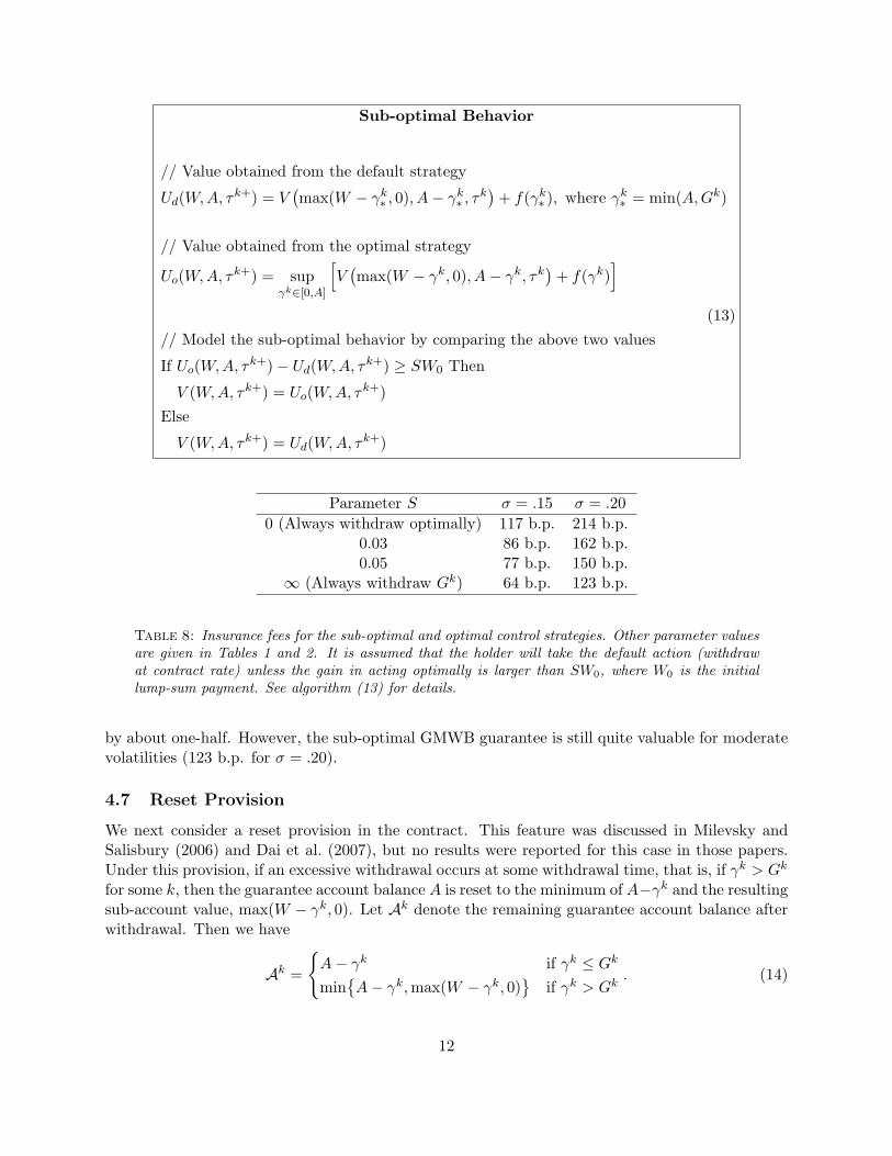
Sub-optimal Behavior

// Value obtained from the default strategy

Ud(W,A, τk+) = V(max(W − γk

∗ , 0), A− γk∗ , τ

k)

+ f(γk∗ ), where γk

∗ = min(A,Gk)

// Value obtained from the optimal strategy

Uo(W,A, τk+) = supγk∈[0,A]

[V

(max(W − γk, 0), A− γk, τk

)+ f(γk)

](13)

// Model the sub-optimal behavior by comparing the above two values

If Uo(W,A, τk+)− Ud(W,A, τk+) ≥ SW0 Then

V (W,A, τk+) = Uo(W,A, τk+)Else

V (W,A, τk+) = Ud(W,A, τk+)

Parameter S σ = .15 σ = .200 (Always withdraw optimally) 117 b.p. 214 b.p.

0.03 86 b.p. 162 b.p.0.05 77 b.p. 150 b.p.

∞ (Always withdraw Gk) 64 b.p. 123 b.p.

Table 8: Insurance fees for the sub-optimal and optimal control strategies. Other parameter valuesare given in Tables 1 and 2. It is assumed that the holder will take the default action (withdrawat contract rate) unless the gain in acting optimally is larger than SW0, where W0 is the initiallump-sum payment. See algorithm (13) for details.

by about one-half. However, the sub-optimal GMWB guarantee is still quite valuable for moderatevolatilities (123 b.p. for σ = .20).

4.7 Reset Provision

We next consider a reset provision in the contract. This feature was discussed in Milevsky andSalisbury (2006) and Dai et al. (2007), but no results were reported for this case in those papers.Under this provision, if an excessive withdrawal occurs at some withdrawal time, that is, if γk > Gk

for some k, then the guarantee account balance A is reset to the minimum of A−γk and the resultingsub-account value, max(W − γk, 0). Let Ak denote the remaining guarantee account balance afterwithdrawal. Then we have

Ak =

{A− γk if γk ≤ Gk

min{A− γk,max(W − γk, 0)

}if γk > Gk

. (14)

12

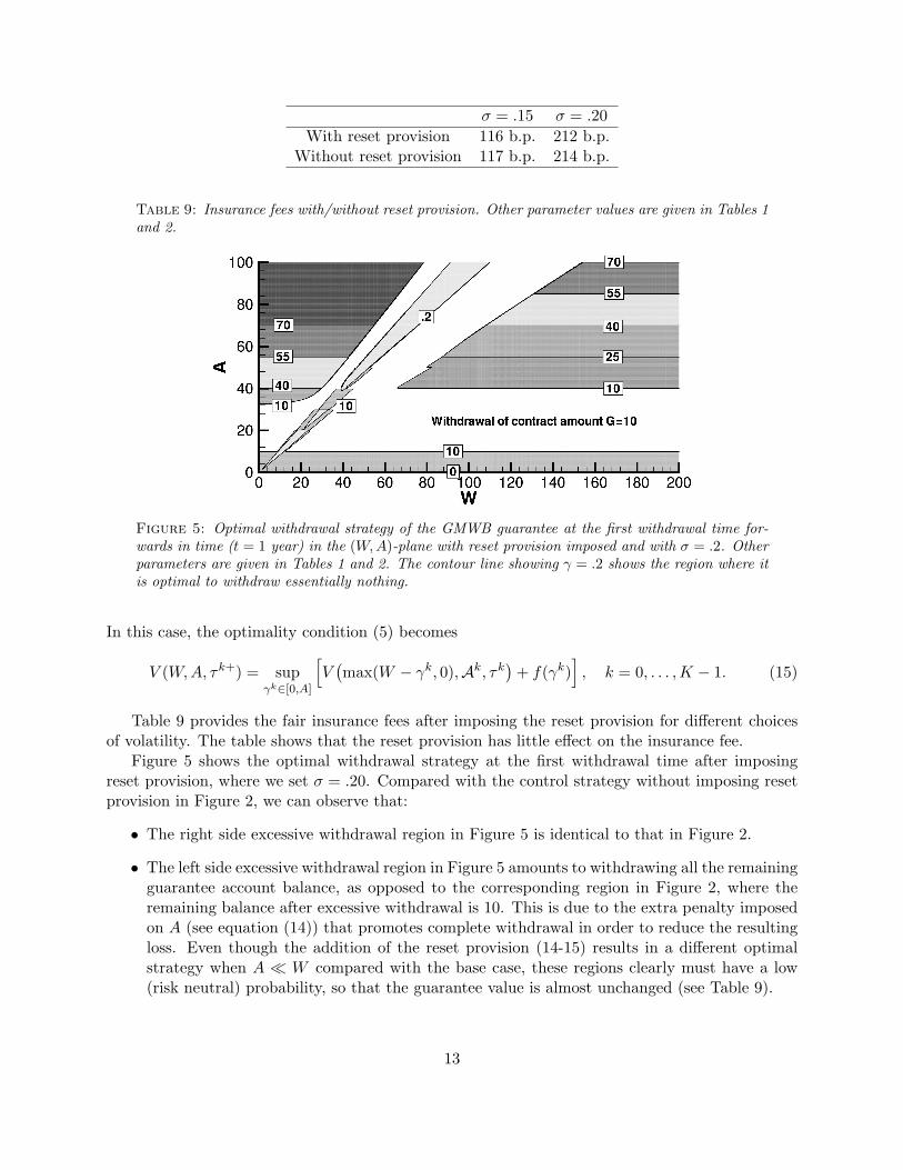
σ = .15 σ = .20With reset provision 116 b.p. 212 b.p.

Without reset provision 117 b.p. 214 b.p.

Table 9: Insurance fees with/without reset provision. Other parameter values are given in Tables 1and 2.

Figure 5: Optimal withdrawal strategy of the GMWB guarantee at the first withdrawal time for-wards in time (t = 1 year) in the (W,A)-plane with reset provision imposed and with σ = .2. Otherparameters are given in Tables 1 and 2. The contour line showing γ = .2 shows the region where itis optimal to withdraw essentially nothing.

In this case, the optimality condition (5) becomes

V (W,A, τk+) = supγk∈[0,A]

[V

(max(W − γk, 0),Ak, τk

)+ f(γk)

], k = 0, . . . ,K − 1. (15)

Table 9 provides the fair insurance fees after imposing the reset provision for different choicesof volatility. The table shows that the reset provision has little effect on the insurance fee.

Figure 5 shows the optimal withdrawal strategy at the first withdrawal time after imposingreset provision, where we set σ = .20. Compared with the control strategy without imposing resetprovision in Figure 2, we can observe that:

• The right side excessive withdrawal region in Figure 5 is identical to that in Figure 2.

• The left side excessive withdrawal region in Figure 5 amounts to withdrawing all the remainingguarantee account balance, as opposed to the corresponding region in Figure 2, where theremaining balance after excessive withdrawal is 10. This is due to the extra penalty imposedon A (see equation (14)) that promotes complete withdrawal in order to reduce the resultingloss. Even though the addition of the reset provision (14-15) results in a different optimalstrategy when A � W compared with the base case, these regions clearly must have a low(risk neutral) probability, so that the guarantee value is almost unchanged (see Table 9).

13

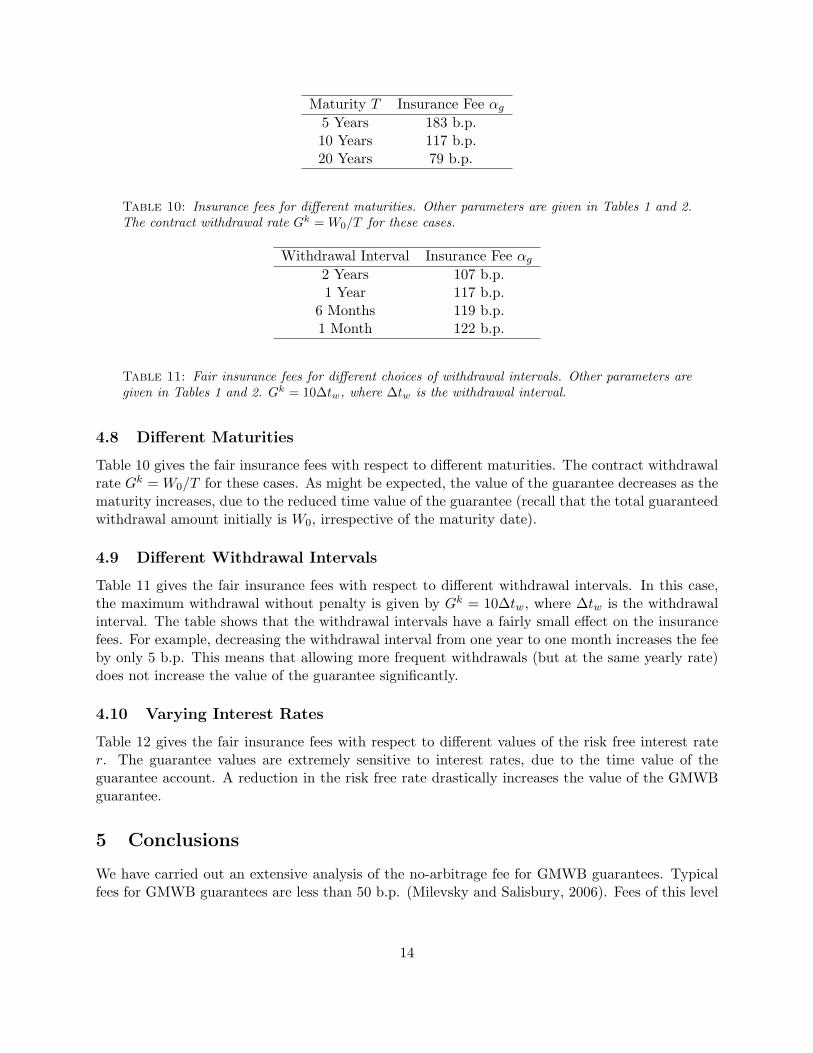
Maturity T Insurance Fee αg

5 Years 183 b.p.10 Years 117 b.p.20 Years 79 b.p.

Table 10: Insurance fees for different maturities. Other parameters are given in Tables 1 and 2.The contract withdrawal rate Gk = W0/T for these cases.

Withdrawal Interval Insurance Fee αg

2 Years 107 b.p.1 Year 117 b.p.

6 Months 119 b.p.1 Month 122 b.p.

Table 11: Fair insurance fees for different choices of withdrawal intervals. Other parameters aregiven in Tables 1 and 2. Gk = 10∆tw, where ∆tw is the withdrawal interval.

4.8 Different Maturities

Table 10 gives the fair insurance fees with respect to different maturities. The contract withdrawalrate Gk = W0/T for these cases. As might be expected, the value of the guarantee decreases as thematurity increases, due to the reduced time value of the guarantee (recall that the total guaranteedwithdrawal amount initially is W0, irrespective of the maturity date).

4.9 Different Withdrawal Intervals

Table 11 gives the fair insurance fees with respect to different withdrawal intervals. In this case,the maximum withdrawal without penalty is given by Gk = 10∆tw, where ∆tw is the withdrawalinterval. The table shows that the withdrawal intervals have a fairly small effect on the insurancefees. For example, decreasing the withdrawal interval from one year to one month increases the feeby only 5 b.p. This means that allowing more frequent withdrawals (but at the same yearly rate)does not increase the value of the guarantee significantly.

4.10 Varying Interest Rates

Table 12 gives the fair insurance fees with respect to different values of the risk free interest rater. The guarantee values are extremely sensitive to interest rates, due to the time value of theguarantee account. A reduction in the risk free rate drastically increases the value of the GMWBguarantee.

5 Conclusions

We have carried out an extensive analysis of the no-arbitrage fee for GMWB guarantees. Typicalfees for GMWB guarantees are less than 50 b.p. (Milevsky and Salisbury, 2006). Fees of this level

14

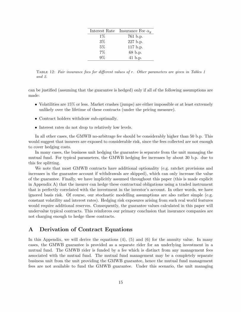
Interest Rate Insurance Fee αg

1% 761 b.p.3% 227 b.p.5% 117 b.p.7% 68 b.p.9% 41 b.p.

Table 12: Fair insurance fees for different values of r. Other parameters are given in Tables 1and 2.

can be justified (assuming that the guarantee is hedged) only if all of the following assumptions aremade:

• Volatilities are 15% or less. Market crashes (jumps) are either impossible or at least extremelyunlikely over the lifetime of these contracts (under the pricing measure).

• Contract holders withdraw sub-optimally.

• Interest rates do not drop to relatively low levels.

In all other cases, the GMWB no-arbitrage fee should be considerably higher than 50 b.p. Thiswould suggest that insurers are exposed to considerable risk, since the fees collected are not enoughto cover hedging costs.

In many cases, the business unit hedging the guarantee is separate from the unit managing themutual fund. For typical parameters, the GMWB hedging fee increases by about 30 b.p. due tothis fee splitting.

We note that most GMWB contracts have additional optionality (e.g. ratchet provisions andincreases in the guarantee account if withdrawals are skipped), which can only increase the valueof the guarantee. Finally, we have implicitly assumed throughout this paper (this is made explicitin Appendix A) that the insurer can hedge these contractual obligations using a traded instrumentthat is perfectly correlated with the investment in the investor’s account. In other words, we haveignored basis risk. Of course, our stochastic modelling assumptions are also rather simple (e.g.constant volatility and interest rates). Hedging risk exposures arising from such real world featureswould require additional reserves. Consequently, the guarantee values calculated in this paper willundervalue typical contracts. This reinforces our primary conclusion that insurance companies arenot charging enough to hedge these contracts.

A Derivation of Contract Equations

In this Appendix, we will derive the equations (4), (5) and (6) for the annuity value. In manycases, the GMWB guarantee is provided as a separate rider for an underlying investment in amutual fund. The GMWB rider is funded by a fee which is distinct from any management feesassociated with the mutual fund. The mutual fund management may be a completely separatebusiness unit from the unit providing the GMWB guarantee, hence the mutual fund managementfees are not available to fund the GMWB guarantee. Under this scenario, the unit managing

15

the guarantee is not permitted to short the mutual fund, and uses an index proxy to hedge theguarantee (Le Roux, 2000). Therefore, it is important to distinguish between these two sets of fees.

We will first derive the equations for the pure GMWB guarantee. We will use the same argu-ments used in Windcliff et al. (2001) to model segregated funds. We then convert these equationsinto the value of the total variable annuity, which can then be related to previous work on GMWBguarantees (Milevsky and Salisbury, 2006; Dai et al., 2007).

Let αm be the proportional fee charged by the manager of the underlying mutual fund. Let αg

be the fee used to fund the GMWB guarantee, with αtot = αm + αg. For simplicity, we will derivethe equations assuming that the underlying asset follows Geometric Brownian Motion.

Consider the following scenario. The underlying asset W in the investor’s account follows

dW = (µ− αtot)Wdt + WσdZ, (16)

where µ is the drift rate and dZ is the increment of a Wiener process. We ignore withdrawals fromthe account in equation (16) for the moment. We assume that the mutual fund tracks an index Wwhich follows the process

dW = µWdt + WσdZ. (17)

We assume that it is not possible to short the mutual fund, so that the obvious arbitrage opportunitycannot be exploited. We further assume that it is possible to track the index W without basis risk.

Now, consider the writer of the GMWB guarantee, with no-arbitrage value U(W,A, t). Theterminal condition is

U(W,A, t = T ) = max(A(1− κ)−W, 0) (18)

which represents the cashflow which must be paid by the guarantee provider. The writer sets upthe hedging portfolio

Π(W, W , t) = −U(W, t) + xW , (19)

where x is the number of units of the index W .Over the time interval t→ t + dt, between withdrawal dates,

dΠ = −[(

Ut + (µ− αtot)WUW +12σ2W 2UWW

)dt + σWUW dZ

]+ x[µWdt + σWdZ] + αgWdt, (20)

where the term (αgWdt) represents the GMWB fee collected by the hedger. Choose

x =W

WUW , (21)

so that equation (20) becomes

dΠ = −[(

Ut − αtotWUW +12σ2W 2UWW

)dt

]+ αgWdt. (22)

Setting dΠ = rΠ dt (since the portfolio is now riskless) gives

Uτ =12σ2W 2UWW + (r − αtot)WUW − rU − αgW, (23)

16

where τ = T − t. Note that equation (23) has the same form as that used to value segregated fundguarantees (Windcliff et al., 2001, 2002).

At withdrawal times τk, the holder of the GMWB will maximize the value of the guarantee, sothat

U(W,A, τk+) = supγk∈[0,A]

[U(max(W − γk, 0), A− γk, τk) + f(γk)−min(γk,W )

]. (24)

Note that

f(γk)−min(γk,W ) =

0 γk ≤ Gk ; γk < W

−κ(γk −Gk) γk > Gk ; γk < W

γk −W γk ≤ Gk ; γk > W

(γk −W )− κ(γk −Gk) γk > Gk ; γk > W

, (25)

which represents the total cash outflows from the writer of the guarantee to the holder of theGMWB contract, i.e. cashflows required to make up any guarantee shortfall net of penalties forwithdrawals above the contract amount.

Now, let V (W,A, τ) be the value of the total variable annuity contract, i.e.

V = U + W. (26)

In other words, V is the total variable annuity value, which includes the amount in the risky accountand the separate GMWB guarantee. Substituting equation (26) into equation (18) gives

V (W,A, τ = 0) = max (W,A(1− κ)) . (27)

Similarly, substituting (26) into (23) gives

Vτ =12σ2W 2VWW + (r − αtot)WVW − rV + αmW, (28)

and finally, at withdrawal times τk we obtain (from equations (26) and (24))

V (W,A, τk+) = supγk∈[0,A]

[V (max(W − γk, 0), A− γk, τk) + f(γk)

]. (29)

Note that if αm = 0, then equations (27 - 29) reduce to the GMWB equations derived in Daiet al. (2007) for the discrete withdrawal case.

Although at first sight the term αmW on the right hand side of equation (28) seems counter-intuitive, we can also derive this equation assuming the following scenario. Imagine that the hedgerreplicates the cash flows associated with the total GMWB contract. In this case, the underlyingmutual fund can be regarded as a purely virtual instrument, following process (16). The hedginginstrument follows process (17), and the hedging unit pays a sales fee of αmW to the mutual fundunit. In other words, rather than having the investor directly pay the proportional fees αm tothe mutual fund unit and αg to the guarantee provider, the investor pays a proportional fee ofαtot = αm + αg to the guarantee provider, which keeps αgW to hedge the guarantee and passesalong αmW to the mutual fund unit. Following a similar argument as in equations (19-23), andnoting that the hedger must pay the mutual fund fees αmW , results in equation (28).

17

References

Andersen, L. and J. Andreasen (2000). Jump-diffusion processes: Volatility smile fitting andnumerical methods for option pricing. Review of Derivatives Research 4, 231–262.

Bauer, D., A. Kling, and J. Russ (2006). A universal pricing framework for guaranteed minimumbenefits in variable annuities. Working paper, Ulm University.

Chen, Z. and P. Forsyth (2007). A numerical scheme for the impulse control formulation for pricingvariable annuities with a Guaranteed Minimum Withdrawal Benefit (GMWB). Submitted toNumerische Mathematik.

Cramer, E., P. Matson, and L. Rubin (2007). Common practices relating to FASB statement 133,Accounting for Derivative Instruments and Hedging Activities as it Relates to Variable Annuitieswith Guaranteed Benefits. Practice Note, American Academy of Actuaries.

Dai, M., Y. K. Kwok, and J. Zong (2007). Guaranteed minimum withdrawal benefit in variableannuities. Mathematical Finance, forthcoming.

d’Halluin, Y., P. Forsyth, and K. Vetzal (2005). Robust numerical methods for contingent claimsunder jump diffusion processes. IMA Journal of Numerical Analysis 25, 65–92.

He, C., J. Kennedy, T. Coleman, P. Forsyth, Y. Li, and K. Vetzal (2006). Calibration and hedgingunder jump diffusion. Review of Derivatives Research 9, 1–35.

Ho, T., S. B. Lee, and Y. Choi (2005). Practical considerations in managing variable annuities.Working paper, Thomas Ho Company.

Kennedy, J., P. Forsyth, and K. Vetzal (2006). Dynamic hedging under jump diffusion with trans-action costs. Submitted to Operations Research.

Le Roux, M. (2000). Private communication. Director of product development, ING InstitutionalMarkets.

Milevsky, M. A. and T. S. Salisbury (2006). Financial valuation of guaranteed minimum withdrawalbenefits. Insurance: Mathematics and Economics 38, 21–38.

Windcliff, H., P. Forsyth, M. Le Roux, and K. Vetzal (2002). Understanding the behaviour andhedging of segregated funds offering the reset feature. North American Actuarial Journal 6,107–125.

Windcliff, H., P. Forsyth, and K. Vetzal (2001). Valuation of segregated funds: shout options withmaturity extensions. Insurance: Mathematics and Economics 29, 1–21.

18