Embed Size (px)
Citation preview

The effects of birth inputs on birthweight:evidence from quantile estimation on panel data
by Jason Abrevaya∗ and Christian M. Dahl†
ABSTRACT
Unobserved heterogeneity among childbearing women makes it difficult to isolate the causal effectsof smoking and prenatal care on birth outcomes (such as birthweight). Whether or not a mothersmokes, for instance, is likely to be correlated with unobserved characteristics of the mother. Thispaper controls for such unobserved heterogeneity by using state-level panel data on maternallylinked births. A quantile-estimation approach, motivated by a correlated random-effects model, isused in order to estimate the effects of smoking and other observables (number of prenatal-carevisits, years of education, etc.) on the entire birthweight distribution.
∗Department of Economics, The University of Texas, Austin, TX 78712.†CREATES and School of Economics and Management, University of Aarhus, Aarhus, Denmark; e-mail:
1 Introduction
Adverse birth outcomes have been found to result in large economic costs, in the form of both
direct medical costs and long-term developmental consequences. It is not surprising, then, that the
public-health community has focused efforts on prenatal-care improvements (e.g., through smoking
cessation, alcohol-intake reduction, and/or better nutrition) that are thought to improve birth out-
comes. Birthweight has served as a leading indicator of infant health, with “low birthweight” (LBW)
infants classified as those weighing less than 2500 grams at birth. Observable measures of poor
prenatal care, such as smoking, have strong negative associations with birthweight. For instance,
according to a report by the Surgeon General, mothers who smoke during pregnancy have babies
that, on average, weigh 250 grams less (Centers for Disease Control and Prevention (2001)).
The direct medical costs of low birthweight are quite high. Based upon hospital-discharge
data from New York and New Jersey, Almond et. al. (2005) report that the hospital costs for
newborns peaks at around $150,000 (in 2000 dollars) for infants that weigh 800 grams; the costs
remain quite high for all “low birthweight” outcomes, with an average cost of around $15,000 for
infants that weigh 2000 grams. The infant-mortality rate also increases at lower birthweights.
Other research has examined the long-term effects of low birthweight on cognitive develop-
ment, educational outcomes, and labor-market outcomes. LBW babies have developmental prob-
lems in cognition, attention, and neuromotor functioning that persist until adolescence (Hack et.
al. (1995)). LBW babies are more likely to delay entry into kindergarten, repeat a grade in school,
and attend special-education classes (Corman (1995); Corman and Chaikind (1998)). LBW babies
are also more likely to have inferior labor-market outcomes, being more likely to be unemployed and
earn lower wages (Behrman and Rosenzweig (2004); Case et. al. (2005); Currie and Hyson (1999)).
Although it has received less attention in the economics literature, high-birthweight out-
comes can also represent adverse outcomes. For instance, babies weighing more than 4000 grams
(classified as high birthweight (HBW)) and especially those weighing more than 4500 grams (clas-
sified as very high birthweight (VHBW)) are more likely to require cesarean-section births, have
higher infant mortality rates, and develop health problems later in life.
A difficulty in evaluating initiatives aimed at improving birth outcomes is to accurately
estimate the causal effects of prenatal activities on these birth outcomes. Unobserved heterogeneity
among childbearing women makes it difficult to isolate causal effects of various determinants of
birth outcomes. Whether or not a mother smokes, for instance, is likely to be correlated with
unobserved characteristics of the mother. To deal with this difficulty, various studies have used
an instrumental-variable approach to estimate the effects of smoking (Evans and Ringel (1999);
Permutt and Hebel (1989)), prenatal care (Currie and Gruber (1996); Evans and Lien (2005);
1

Joyce (1999)), and air pollution (Chay and Greenstone (2003a, 2003b)) on birth outcomes.
Another approach has been to utilize panel data (i.e., several births for each mother) to iden-
tify these effects from changes in prenatal behavior or maternal characteristics between pregnancies
(Abrevaya (2006); Currie and Moretti (2002); Rosenzweig and Wolpin (1991); Royer (2004)). One
concern with the panel-data identification strategy is the presence of “feedback effects,” specifically
that prenatal care and smoking in later pregnancies may be correlated with birth outcomes in ear-
lier pregnancies. Royer (2004) provides an explicit estimation strategy to deal with such feedback
effects (using data on at least three births per mother). Abrevaya (2006) shows that feedback
effects are likely to cause the estimated (negative) smoking effect to be too large in magnitude.
Since the costs associated with birthweight have been found to exist primarily at the low end
of the birthweight distribution (with costs increasing significantly at the very low end), most studies
have estimated the effects of birth inputs on the fraction of births below various thresholds (e.g.,
2500 grams for LBW and 1500 grams for “very low birthweight”). As an alternative, this paper
considers a quantile-regression approach to estimating the effects of birth inputs on birthweight,
so it is useful to compare the two approaches. The threshold-crossing approach fixes a common
unconditional threshold for the entire sample, whereas the quantile-regression approach focuses
upon particular conditional quantiles of the birthweight distribution. Denoting birthweight by bw
and a birth input vector by x, a probit-based threshold-crossing model for LBW outcomes would
be Pr(bw < 2500|x) = Φ(x′γ). For each x, there is a conditional probability of the LBW outcome
(bw below the common threshold) and estimates of γ can be used to infer the marginal effects of
the birth inputs upon these conditional probabilities. For the quantile approach, a simple (linear)
model for, say, the 5% conditional quantile would be Q5%(bw|x) = x′β. The value of the conditional
quantile Q5%(bw|x) may be below the LBW threshold of 2500 grams for some x values and above it
for other x values. The estimated marginal effects (inferred from the estimates of β) would indicate
how the 5% conditional quantile would be affected at all x values. These effects are not directly
comparable to the probit-based effects.
For the question of economic costs, both the probit approach and quantile approach have
drawbacks: (i) the probit approach is inherently discontinuous and offers only predictions of LBW
vs. non-LBW outcomes, and (ii) the quantile approach combines predictions from extremely ad-
verse x values (lower Q5%(bw|x)), where the costs are higher, and less adverse x values (higher
Q5%(bw|x)), where the costs are lower. For the question of what causes LBW outcomes, the simple
probit-based approach is certainly sufficient. The quantile approach, however, provides a convenient
method for determining how birth inputs affect birthweight at different parts of the distribution.
The closest analogy with the threshold-crossing approach would be to continuously alter the thresh-
old value and estimate a series of probit models. Given the different aspects of the birthweight
2

distribution being modeled and estimated by the two approaches, our view is that these approaches
should be viewed as complements to each other rather than substitutes.
A recent literature on estimation of quantile treatment effects, including Abadie, Angrist,
and Imbens (2002) and Bitler, Gelbach, and Hoynes (2006), has argued that traditional estimation
of average (mean) treatment effects may miss important causal impacts. Specifically, an aver-
age treatment effect inherently combines the magnitudes of causal effects upon different parts of
the conditional distribution. It is quite possible, as in our birthweight application (and also in
wage-distribution applications), that societal costs and benefits are more pronounced at the lower
quantiles of the conditional distribution. As an example, if one estimated the average causal effect
of smoking to be a reduction in birthweight of 150 grams, it could be the case that the effect of
smoking on lower quantiles is substantially higher or lower than 150 grams. If a 200-gram effect
were estimated at lower quantiles and a 100-gram effect at higher quantiles, this would argue for
a stronger policy response than if the effects were instead stronger at the higher quantiles. Ulti-
mately, consideration of how effects vary over the quantiles is an empirical question and one which
we attempt to answer in the context of birthweight regressions in this paper.
Previous quantile-estimation approaches to estimating birth-outcome regressions have used
cross-sectional data and, therefore, have suffered from an inability to control for unobserved
heterogeneity. For instance, Abrevaya (2001) (see also Koenker and Hallock (2001) and Cher-
nozhukov (2005)) uses cross-sectional federal natality data and finds that various observables have
significantly stronger associations with birthweight at lower quantiles of the birthweight distribu-
tion; unfortunately, one can not interpret these “effects” as causal since the estimation has a purely
reduced-form structure that does not account for unobserved heterogeneity.
The outline of the paper is as follows. Section 2 details the quantile-estimation approach,
motivated by the “correlated random effects model” of Chamberlain (1982, 1984). We consider a
notion of marginal effects upon conditional quantiles in which we explicitly control for unobserved
heterogeneity by allowing the “mother random effect” to be related to observables. Section 3
describes the maternally-linked birth panel data for Washington and Arizona that are used in
this study. Section 4 reports the main empirical results of the paper. There are some interesting
differences between the panel-data and cross-sectional results. For example, the results from panel-
data estimation, which controls for unobserved heterogeneity, indicate that the negative effects of
smoking on birthweight are significantly lower (in magnitude) across all quantiles than indicated
by the cross-sectional estimates. Section 4.2 provides a general hypothesis testing framework.
Section 4.3 discusses issues related to endogeneity (e.g., feedback effects and measurement error) in
the panel-data context. Section 5 discusses the theoretical panel-data model in greater detail and
highlights directions for future research.
3

2 Quantile estimation for two-birth panel data
Despite the widespread use of both panel-data methodology and quantile-regression methodology,
there has been little work at the intersection of the two methodologies. As discussed in this section,
the most likely explanation is the difficulty in extending differencing methods to quantiles. The
outline of this section is as follows. Section 2.1 briefly reviews the fixed effects and correlated
random effects models for conditional expectations. Building upon the correlated random effects
framework of Section 2.1, Section 2.2 extends the notion of marginal effects (and their estimation)
to conditional quantile models. Section 2.3 discusses previous related studies.
2.1 Review of conditional expectation models with panel data
Suppose that the data source contains information on exactly two births for a large sample of
mothers. A standard linear panel-data model for such a situation would be
ymb = x′mbβ + cm + umb (b = 1, 2; m = 1, . . . ,M), (1)
where m indexes mothers, b indexes births, y denotes a birth outcome (e.g., birthweight), x denotes
a vector of observables, c denotes the (unobservable) “mother effect,” and u denotes a birth-specific
disturbance. To simplify notation, let xm ≡ (xm1, xm2) denote the covariate values from both births
of a given mother. From the basic model in (1), several different types of panel-data models arise
from the assumptions concerning the unobservable cm. In the “pure” random-effects version of (1),
cm is assumed to be uncorrelated with xm. This assumption is implausible in the context of our
empirical application, so attention is focused upon two models that allow for dependence between
cm and xm: (1) the fixed-effects model and (2) the correlated random-effects model.
Fixed-effects model: The fixed-effects model allows correlation between cm and xm in a com-
pletely unspecified manner. The “meaning” of the parameter vector β is given by
β =∂E(ymb|xm, cm)
∂xmb(2)
under the following assumption:
(A1) E(um1|xm, cm) = E(um2|xm, cm) = 0 ∀m. (3)
It is well known that, under (A1), β can be consistently estimated by a first-difference regression
(i.e., regressing ym2 − ym1 on xm2 − xm1). The reason that this strategy works for the conditional
expectation hinges critically upon the fact that an expectation is a linear operator, a property that
is not shared by conditional quantiles.
4

Correlated random-effects model: The correlated random-effects model of Chamberlain (1982,
1984) views the unobservable cm as a linear projection onto the observables plus a disturbance:
cm = ψ + x′m1λ1 + x′
m2λ2 + vm, (4)
where ψ is a scalar and vm is a disturbance that (by definition of linear projections) is uncorrelated
with xm1 and xm2. Combining equations (1) and (4) yields
ym1 = ψ + x′m1(β + λ1) + x′
m2λ2 + vm + um1 (5)
ym2 = ψ + x′m1λ1 + x′
m2(β + λ2) + vm + um2. (6)
The parameters (ψ, β, λ1, λ2) in (5) and (6) can be estimated by least-squares regression or other
methods (see, e.g., Wooldridge (2002, Section 11.3)). The vector xm1 affects ym1 through two
channels, (i) a direct effect (expressed by the x′m1β term) and (ii) an indirect effect working through
the unobservable effect cm. In contrast, the vector xm1 affects ym2 only through the unobservable
effect cm. In fact, under the additional assumption
(A2) E(vm|xm) = 0, (7)
the “meaning” of β is given by the following equation
β =∂E(ym1|xm)
∂xm1− ∂E(ym2|xm)
∂xm1=∂E(ym2|xm)
∂xm2− ∂E(ym1|xm)
∂xm2. (8)
That is, β tells us how much xm1 affects E(ym1|xm) above and beyond the effect that works through
the unobservable cm.
2.2 Estimation of effects on conditional quantiles with panel data
For conditional quantiles, a simple differencing strategy is infeasible since quantiles are not linear
operators — that is, in general, Qτ (ym2 − ym1|xm) �= Qτ (ym2|xm) − Qτ (ym1|xm), where Qτ (·|·)denotes the τ -th conditional quantile function for τ ∈ (0, 1). This inherent difficulty has been
recognized by others and is summarized nicely in a recent quantile-regression survey by Koenker
and Hallock (2000): “Quantiles of convolutions of random variables are rather intractable objects,
and preliminary differencing strategies familiar from Gaussian models have sometimes unanticipated
effects.” Without being more explicit about the relationship between cm and xm, it is difficult to
envision an appropriate strategy for dealing with conditional quantiles, although Koenker (2004)
has made some progress on this front.
To consider the relevant effects of the observables on the conditional quantiles Qτ (ymb|xm)
(rather than E(ymb|xm)), we consider the analogous effects to those given in equation (8). In
5
particular, the effects of the observables on a given conditional quantile are given by
∂Qτ (ym1|xm)∂xm1
− ∂Qτ (ym2|xm)∂xm1
(9)
and∂Qτ (ym2|xm)
∂xm2− ∂Qτ (ym1|xm)
∂xm2. (10)
For example, the difference in equation (9) is the effect of xm1 (first-birth observables) onQτ (ym1|xm)
above and beyond the effect on the τ -th conditional quantile that works through the unobservable.
To estimate the effects given in equations (9) and (10), a model for both Qτ (ym1|xm) and
Qτ (ym2|xm) is needed. Unfortunately, it is non-trivial to explicitly determine the conditional quan-
tile models. Consider, for example, the simple case in which the data-generating process is given
by equations (1) and (4) (which then imply equations (5) and (6)). If all of the error disturbances
(um1, um2, vm) were independent of xm, then the conditional quantile functions would take a simple
form (analogous to that of the conditional expectation function under assumption (A2)):
Qτ (ym1|xm) = ψ1τ + x′
m1(β + λ1) + x′m2λ2 (11)
Qτ (ym2|xm) = ψ2τ + x′
m1λ1 + x′m2(β + λ2). (12)
Under this independence assumption, the effect of the disturbances is reflected by a locational shift
in the conditional quantiles (ψ1τ and ψ2
τ ); the slopes do not vary across the conditional quantiles.
Without the independence assumption, however, the simple linear form for the conditional quantile
functions (like those in equations (11) and (12)) only arises in very special cases. In general, the
conditional quantile functions involve more complicated non-linear expressions and, in fact, can not
be explicitly written down without a complete parametric specification of the error disturbances.
Therefore, the conditional quantiles are viewed as somewhat general functions of xm: say,
Qτ (ym1|xm) = f1τ (xm) and Qτ (ym2|xm) = f2
τ (xm). To estimate the effects in (9) and (10), then,
reduced-form models for Qτ (ym1|xm) and Qτ (ym2|xm) are specified. These reduced-form models
should be viewed as approximating the “true” conditional quantile functions f1τ (xm) and f2
τ (xm).
In this paper, a very simple form for the reduced-form models is considered, in which the conditional
quantiles are expressed as linear (and separable) functions of xm1 and xm2:
Qτ (ym1|xm) = φ1τ + x′
m1θ1τ + x′
m2λ2τ (13)
Qτ (ym2|xm) = φ2τ + x′
m1λ1τ + x′
m2θ2τ . (14)
A more general model, as well as the appropriateness of linearity and separability, is discussed
in greater detail in Section 5. Based upon (13) and (14), the effects of the observables on the
conditional quantiles (see (9) and (10)) are equal to θ1τ − λ1
τ (for the first-birth outcome) and
6

θ2τ − λ2
τ (for the second-birth outcome). The parameters (φ1τ , φ
2τ , θ
1τ , θ
2τ , λ
1τ , λ
2τ ) can be consistently
estimated with linear quantile regression (Koenker and Bassett (1978)).
Although the linear approximation may at first appear to be restrictive, this strategy is the
one usually employed in cross-sectional quantile regression. In the cross-sectional case, even if the
data-generating process is linear in the covariates with a mean-zero error, the conditional quantiles
will only be linear in the covariates in very special cases (see, e.g., Koenker and Bassett (1982)).
Even in cross-sectional applications, then, the specification chosen by an empirical researcher (lin-
ear usually) should also be viewed as a reduced-form approximation to the true conditional quantile
function. In fact, empirical applications of quantile regression generally start (either explicitly or
implicitly) with a reduced-form approximating model of the conditional quantile function rather
than the data-generating process (see, e.g., Buchinsky (1994) and Bassett and Chen (2001)). An-
grist, Chernozhukov, and Fernandez-Val (2006) provide a framework for analyzing misspecification
of the conditional quantile function. Although beyond the scope of this paper, it would be inter-
esting to apply their methodology to the panel-data setting considered here.
The linear approximation approach is also an inherent feature of the correlated random-
effects approach for the conditional expectation model given by (1) and (4). As Chamberlain (1982)
originally pointed out, if assumption (A2) does not hold, the conditional expectation function is
non-linear; in this case, equations (5) and (6) represent linear approximations (projections) and β
represents the marginal effects of the covariates upon these linear approximations.
For the application in this paper, we impose the additional restriction that the effects on
the conditional quantiles are the same for both birth outcomes. This restriction is similar to the
implicit restriction embodied in the linear panel-data model (1), where β does not vary with b. For
the conditional quantiles, let βτ denote the (common) effect vector, so that the restriction is
βτ = θ1τ − λ1
τ = θ2τ − λ2
τ . (15)
Under this restriction, the conditional quantile functions in (13) and (14) can be re-written as
Qτ (ym1|xm) = φ1τ + x′
m1(βτ + λ1τ ) + x′
m2λ2τ = φ1
τ + x′m1βτ + x′
m1λ1τ + x′
m2λ2τ (16)
Qτ (ym2|xm) = φ2τ + x′
m1λ1τ + x′
m2(βτ + λ2τ ) = φ2
τ + x′m2βτ + x′
m1λ1τ + x′
m2λ2τ . (17)
The simplest estimation strategy, based upon the second equalities in both (16) and (17), is to run
a pooled linear quantile regression in which the observations corresponding to both births of a given
mother are stacked together as a pair. In particular, a quantile regression (using the estimator for
7
the τ -th quantile) would be run using⎡⎢⎢⎢⎢⎢⎢⎢⎢⎢⎢⎢⎢⎢⎢⎢⎣
y11y12· · ·y21y22· · ·...
· · ·yM1yM2
⎤⎥⎥⎥⎥⎥⎥⎥⎥⎥⎥⎥⎥⎥⎥⎥⎦
and
⎡⎢⎢⎢⎢⎢⎢⎢⎢⎢⎢⎢⎢⎢⎢⎢⎣
1 0 x′11 x′
11 x′12
1 1 x′12 x′
11 x′12
· · · · · · · · · · · · · · ·1 0 x′
21 x′21 x′
221 1 x′
22 x′21 x′
22· · · · · · · · · · · · · · ·
...· · · · · · · · · · · · · · ·1 0 x′
M1 x′M1 x′
M21 1 x′
M2 x′M1 x′
M2
⎤⎥⎥⎥⎥⎥⎥⎥⎥⎥⎥⎥⎥⎥⎥⎥⎦
(18)
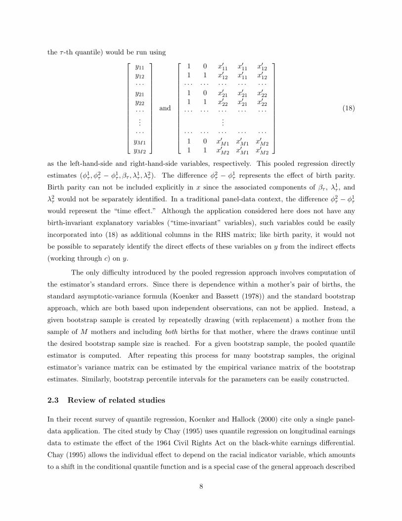
as the left-hand-side and right-hand-side variables, respectively. This pooled regression directly
estimates (φ1τ , φ
2τ − φ1
τ , βτ , λ1τ , λ
2τ ). The difference φ2
τ − φ1τ represents the effect of birth parity.
Birth parity can not be included explicitly in x since the associated components of βτ , λ1τ , and
λ2τ would not be separately identified. In a traditional panel-data context, the difference φ2
τ − φ1τ
would represent the “time effect.” Although the application considered here does not have any
birth-invariant explanatory variables (“time-invariant” variables), such variables could be easily
incorporated into (18) as additional columns in the RHS matrix; like birth parity, it would not
be possible to separately identify the direct effects of these variables on y from the indirect effects
(working through c) on y.
The only difficulty introduced by the pooled regression approach involves computation of
the estimator’s standard errors. Since there is dependence within a mother’s pair of births, the
standard asymptotic-variance formula (Koenker and Bassett (1978)) and the standard bootstrap
approach, which are both based upon independent observations, can not be applied. Instead, a
given bootstrap sample is created by repeatedly drawing (with replacement) a mother from the
sample of M mothers and including both births for that mother, where the draws continue until
the desired bootstrap sample size is reached. For a given bootstrap sample, the pooled quantile
estimator is computed. After repeating this process for many bootstrap samples, the original
estimator’s variance matrix can be estimated by the empirical variance matrix of the bootstrap
estimates. Similarly, bootstrap percentile intervals for the parameters can be easily constructed.
2.3 Review of related studies
In their recent survey of quantile regression, Koenker and Hallock (2000) cite only a single panel-
data application. The cited study by Chay (1995) uses quantile regression on longitudinal earnings
data to estimate the effect of the 1964 Civil Rights Act on the black-white earnings differential.
Chay (1995) allows the individual effect to depend on the racial indicator variable, which amounts
to a shift in the conditional quantile function and is a special case of the general approach described
8
in Section 2.2. Interestingly, the application of Chay (1995) involves censored earnings data, so that
quantile regression methods for censored data (Powell (1984, 1986)) are needed. Such censored-
data quantile methods would also work with the general model of Section 2.2 but are not needed
for the application considered in this paper.
A more recent application of quantile regression on panel data is Arias et. al. (2001), who
estimate the returns to schooling using twins data. To deal with the unobserved “family effect,”
the authors include proxy variables (father’s education and sibling’s education) in the model. This
proxy-variable approach is related to the correlated random effects model in the sense that the latter
specification can be viewed as using the observables xm1 and xm2 as proxies for the unobserved
individual effect. One could also incorporate an external proxy (such as father’s education in the
Arias et. al. (2001) case) into the correlated random effects framework.
Another panel-data study that is directly related to our empirical application is Royer (2004),
who applies a correlated random effects model to maternally linked data from Texas. Royer (2004)
estimates the effects of various observables (with a focus upon maternal age) on “binary” birth
outcomes (such as premature birth or LBW birth). Fixed-effects estimation is also possible (in the
context of the linear probability model) whereas no such alternative is available in the conditional
quantile case. Royer (2004) also relaxes the strict exogeneity assumption (required for consistency
of the fixed-effects estimator) in several interesting ways. Unfortunately, identification of the least
restrictive models requires panel data with at least three births per mother. As a practical matter,
this requirement reduces the sample size to an extent that makes the estimated effects of observ-
ables rather imprecise and introduces a possible selection bias (see the discussion in Royer (2004,
pp. 39ff)). Analogous extensions to the conditional quantile models are left for future research.
3 Data
Detailed “natality data” are recorded for nearly every live birth in the United States. Information
on maternal characteristics (age, education, race, etc.), birth outcomes (birthweight, gestation,
etc.), and prenatal care (number of prenatal visits, smoking status, etc.) is collected by each state
(with federal guidelines on specific data-item requirements). Unfortunately, due to confidentiality
restrictions, comprehensive natality data with personal identifiers are not available at the federal
level, making it difficult to reliably construct maternally-linked panel data. However, individual
states may release such personal identifiers to researchers, subject to confidentiality agreements in
most cases. The data used in this study were obtained from two states, Washington and Arizona,
and are described in detail below:
9

1. Washington data: The Washington State Longitudinal Birth Database (WSLBD) was pro-
vided by Washington’s Center for Health Statistics. The WSLBD is a panel dataset consisting
of all births between 1992 and 2002 that could be accurately linked together as belonging to
the same mother. (The original WSLBD has births dating back to 1980, but mother’s edu-
cation is not available as a data item until 1992.) The matching algorithm used to construct
the WSLBD used personal identifying information such as mother’s full maiden name and
mother’s date of birth. For two births to be linked together, (i) an exact match on mother’s
name, mother’s date of birth, mother’s race, and mother’s state of birth was required, and
(ii) consistency of birth parity and the reported interval-since-last-birth was required. Only
births that could be uniquely linked together were retained in the WSLBD.
2. Arizona data: The Arizona Department of Health Services provided the authors with data
on all births occurring in the state of Arizona between 1993 and 2002. Although names were
not provided, the exact dates of birth for both mother and father were provided in the data.
To maternally link births together, we followed as closely as possible the algorithm used for
the Washington data. For two births to be linked together, (i) an exact match on mother’s
date of birth, father’s date of birth, mother’s race, and mother’s state of birth was required,
and (ii) consistency of birth parity and the reported interval-since-last-birth was required. As
with the Washington data, only births that could be uniquely linked together were retained.
Since births could not be linked by maternal name, we decided to also require an exact match
on father’s date of birth in order to minimize the chance of false matches entering the sample.
(Roughly 3.5% of births that were linked on the basis of mother’s birthdate are dropped
when links are also based upon father’s birthdate.) This choice turns out to have very little
impact on the estimation results reported in Section 4. The decision to match upon father’s
birthdate restricts the Arizona sample to mothers whose children had the same birth father,
which is not a restriction of the Washington sample.
For this study, we consider only pairs of first and second births to white mothers. Birth
outcomes (and the effects of other variables upon birth outcomes) have been found to differ across
different races and at higher birth parities. The choice of subsample circumvents these issue by fo-
cusing upon a more homogeneous sample. The resulting estimates, of course, should be interpreted
as being applicable to the subpopulation represented by this sample choice.
Estimation was carried out separately for the Washington data and Arizona data. The
Washington data has several advantages over the Arizona data: (i) the matching of siblings for the
Washington data is of higher quality due to the use of mothers’ names, (ii) the Washington data is
not restricted to siblings with the same fathers, and (iii) the Washington data includes information
10
on the month of first prenatal visit. For these reasons, most of the detailed analysis will be reported
for the Washington data. Results for Arizona will be discussed more briefly, but these results serve
as a useful comparison to the Washington results.
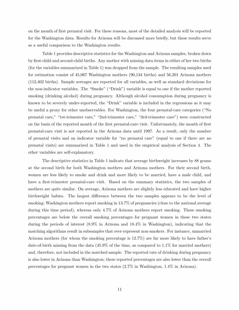
Table 1 provides descriptive statistics for the Washington and Arizona samples, broken down
by first-child and second-child births. Any mother with missing data items in either of her two births
(for the variables summarized in Table 1) was dropped from the sample. The resulting samples used
for estimation consist of 45,067 Washington mothers (90,134 births) and 56,201 Arizona mothers
(112,402 births). Sample averages are reported for all variables, as well as standard deviations for
the non-indicator variables. The “Smoke” (“Drink”) variable is equal to one if the mother reported
smoking (drinking alcohol) during pregnancy. Although alcohol consumption during pregnancy is
known to be severely under-reported, the “Drink” variable is included in the regressions as it may
be useful a proxy for other unobservables. For Washington, the four prenatal-care categories (“No
prenatal care,” “1st-trimester care,” “2nd-trimester care,” “3rd-trimester care”) were constructed
on the basis of the reported month of the first prenatal-care visit. Unfortunately, the month of first
prenatal-care visit is not reported in the Arizona data until 1997. As a result, only the number
of prenatal visits and an indicator variable for “no prenatal care” (equal to one if there are no
prenatal visits) are summarized in Table 1 and used in the empirical analysis of Section 4. The
other variables are self-explanatory.
The descriptive statistics in Table 1 indicate that average birthweight increases by 88 grams
at the second birth for both Washington mothers and Arizona mothers. For their second birth,
women are less likely to smoke and drink and more likely to be married, have a male child, and
have a first-trimester prenatal-care visit. Based on the summary statistics, the two samples of
mothers are quite similar. On average, Arizona mothers are slightly less educated and have higher
birthweight babies. The largest difference between the two samples appears to be the level of
smoking: Washington mothers report smoking in 13.7% of pregnancies (close to the national average
during this time period), whereas only 4.7% of Arizona mothers report smoking. These smoking
percentages are below the overall smoking percentages for pregnant women in these two states
during the periods of interest (8.9% in Arizona and 18.4% in Washington), indicating that the
matching algorithms result in subsamples that over-represent non-smokers. For instance, unmarried
Arizona mothers (for whom the smoking percentage is 12.7%) are far more likely to have father’s
date-of-birth missing from the data (45.9% of the time, as compared to 1.1% for married mothers)
and, therefore, not included in the matched sample. The reported rate of drinking during pregnancy
is also lower in Arizona than Washington; these reported percentages are also lower than the overall
percentages for pregnant women in the two states (2.7% in Washington, 1.4% in Arizona).
11
Table 1: Descriptive Statistics, Washington and Arizona Birth Panels
Variable Washington Arizona1st Child 2nd Child 1st Child 2nd Child
Birthweight (in grams) 3442 (523) 3530 (536) 3339 (517) 3427 (505)Male child 0.515 0.511 0.520 0.516Mother’s age 25.27 (5.25) 27.89 (5.35) 25.23 (5.26) 27.85 (5.36)Mother’s education 13.52 (2.32) 13.72 (2.21) 13.21 (2.68) 13.39 (2.61)Married 0.751 0.853 0.780 0.886No prenatal care 0.004 0.003 0.005 0.0061st-trimester care 0.879 0.895 — —2nd-trimester care 0.107 0.093 — —3rd-trimester care 0.014 0.012 — —Smoke 0.143 0.132 0.049 0.044Drink 0.017 0.014 0.009 0.007# prenatal visits 12.06 (3.53) 11.63 (3.25) 11.83 (3.59) 11.73 (3.55)Quantiles of birthweight:
10% quantile 2807 2892 2750 286325% quantile 3146 3220 3061 314650% quantile 3458 3543 3373 344575% quantile 3770 3855 3685 374290% quantile 4060 4167 3968 4040
# of Observations 45,067 45,067 56,201 56,201
12
Table 1 also provides the (unconditional) 10%/25%/50%/75%/90% quantiles for first and
second births in Washington and Arizona. These quantiles indicate fairly symmetric birthweight
distributions, with the median quite close to the mean, the 25% and 75% quantiles roughly equidis-
tant from the median, and the 10% and 90% quantiles roughly equidistant from the median. For
both states, there is a positive shift in the entire birthweight distribution from first to second births.
The shift is largest in magnitude at the 90% quantile (107 grams) for Washington births and at the
10% quantile (113 grams) for Arizona births. Finally, we note that the LBW cutoff of 2500 grams
corresponds to the 3–5% quantiles of the unconditional birthweight distributions, whereas the HBW
cutoff of 4000 grams corresponds to the 85–92% quantiles of the unconditional distributions.
4 Results
Regression results for the two maternally linked datasets are provided in Section 4.1, within the
strict-exogeneity framework introduced in Section 2. A straightforward approach to hypothesis
testing is provided in Section 4.2. Section 4.3 provides discussion related to possible violations of
strict exogeneity (e.g., feedback effects or mismeasured variables).
4.1 Regression results
In the interest of space, the full set of numerical results (tables) and a detailed discussion are
provided only for the Washington data (Section 4.1.1). The Arizona results are reported in a
graphical format comparable to the Washington results (Section 4.1.3), but the detailed tables have
been omitted and the discussion is limited to comparisons with the Washington results. (Complete
tables are available upon request from the authors.)
4.1.1 Washington data
The tables report estimates for the quantiles τ ∈ {0.10, 0.25, 0.50, 0.75, 0.90} (along with least-
squares estimates for comparison), although the figures presented in this section consider marginal
effects at 2-percent intervals (specifically, τ ∈ {0.04, 0.06, . . . , 0.94, 0.96}). Throughout this section,
the dependent variable of interest is birthweight (measured in grams). In order to have a relevant
comparison for the panel-data results, cross-sectional results (without incorporating the correlated
random effects) are also reported. For the cross-sectional results, the panel structure of the data
is only used for computing standard errors. Since each mother appears twice in the data, the
pair-sampling bootstrap described at the end of Section 2.2 is used.
Tables 2 and 3 report the cross-sectional results and panel-data results, respectively. The
model specification includes the variables summarized in Table 1, along with an indicator variable
13
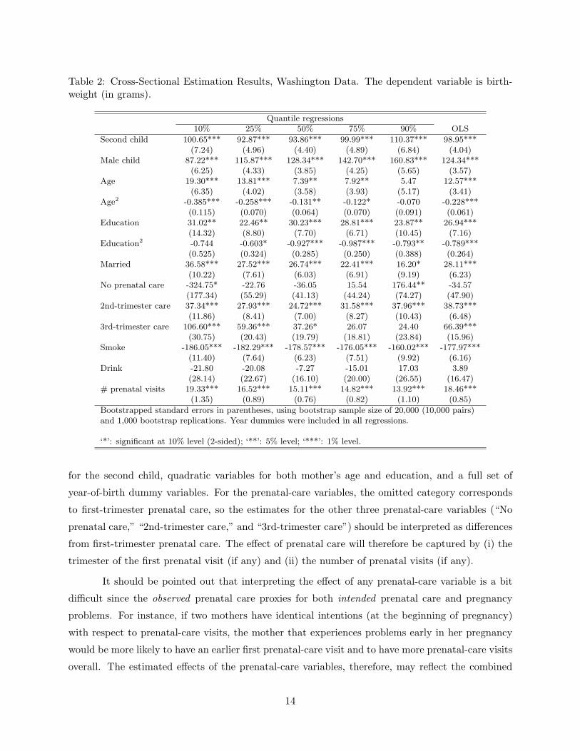
Table 2: Cross-Sectional Estimation Results, Washington Data. The dependent variable is birth-weight (in grams).
Quantile regressions10% 25% 50% 75% 90% OLS
Second child 100.65*** 92.87*** 93.86*** 99.99*** 110.37*** 98.95***(7.24) (4.96) (4.40) (4.89) (6.84) (4.04)
Male child 87.22*** 115.87*** 128.34*** 142.70*** 160.83*** 124.34***(6.25) (4.33) (3.85) (4.25) (5.65) (3.57)
Age 19.30*** 13.81*** 7.39** 7.92** 5.47 12.57***(6.35) (4.02) (3.58) (3.93) (5.17) (3.41)
Age2 -0.385*** -0.258*** -0.131** -0.122* -0.070 -0.228***(0.115) (0.070) (0.064) (0.070) (0.091) (0.061)
Education 31.02** 22.46** 30.23*** 28.81*** 23.87** 26.94***(14.32) (8.80) (7.70) (6.71) (10.45) (7.16)
Education2 -0.744 -0.603* -0.927*** -0.987*** -0.793** -0.789***(0.525) (0.324) (0.285) (0.250) (0.388) (0.264)
Married 36.58*** 27.52*** 26.74*** 22.41*** 16.20* 28.11***(10.22) (7.61) (6.03) (6.91) (9.19) (6.23)
No prenatal care -324.75* -22.76 -36.05 15.54 176.44** -34.57(177.34) (55.29) (41.13) (44.24) (74.27) (47.90)
2nd-trimester care 37.34*** 27.93*** 24.72*** 31.58*** 37.96*** 38.73***(11.86) (8.41) (7.00) (8.27) (10.43) (6.48)
3rd-trimester care 106.60*** 59.36*** 37.26* 26.07 24.40 66.39***(30.75) (20.43) (19.79) (18.81) (23.84) (15.96)
Smoke -186.05*** -182.29*** -178.57*** -176.05*** -160.02*** -177.97***(11.40) (7.64) (6.23) (7.51) (9.92) (6.16)
Drink -21.80 -20.08 -7.27 -15.01 17.03 3.89(28.14) (22.67) (16.10) (20.00) (26.55) (16.47)
# prenatal visits 19.33*** 16.52*** 15.11*** 14.82*** 13.92*** 18.46***(1.35) (0.89) (0.76) (0.82) (1.10) (0.85)
Bootstrapped standard errors in parentheses, using bootstrap sample size of 20,000 (10,000 pairs)and 1,000 bootstrap replications. Year dummies were included in all regressions.
‘*’: significant at 10% level (2-sided); ‘**’: 5% level; ‘***’: 1% level.
for the second child, quadratic variables for both mother’s age and education, and a full set of
year-of-birth dummy variables. For the prenatal-care variables, the omitted category corresponds
to first-trimester prenatal care, so the estimates for the other three prenatal-care variables (“No
prenatal care,” “2nd-trimester care,” and “3rd-trimester care”) should be interpreted as differences
from first-trimester prenatal care. The effect of prenatal care will therefore be captured by (i) the
trimester of the first prenatal visit (if any) and (ii) the number of prenatal visits (if any).
It should be pointed out that interpreting the effect of any prenatal-care variable is a bit
difficult since the observed prenatal care proxies for both intended prenatal care and pregnancy
problems. For instance, if two mothers have identical intentions (at the beginning of pregnancy)
with respect to prenatal-care visits, the mother that experiences problems early in her pregnancy
would be more likely to have an earlier first prenatal-care visit and to have more prenatal-care visits
overall. The estimated effects of the prenatal-care variables, therefore, may reflect the combined
14
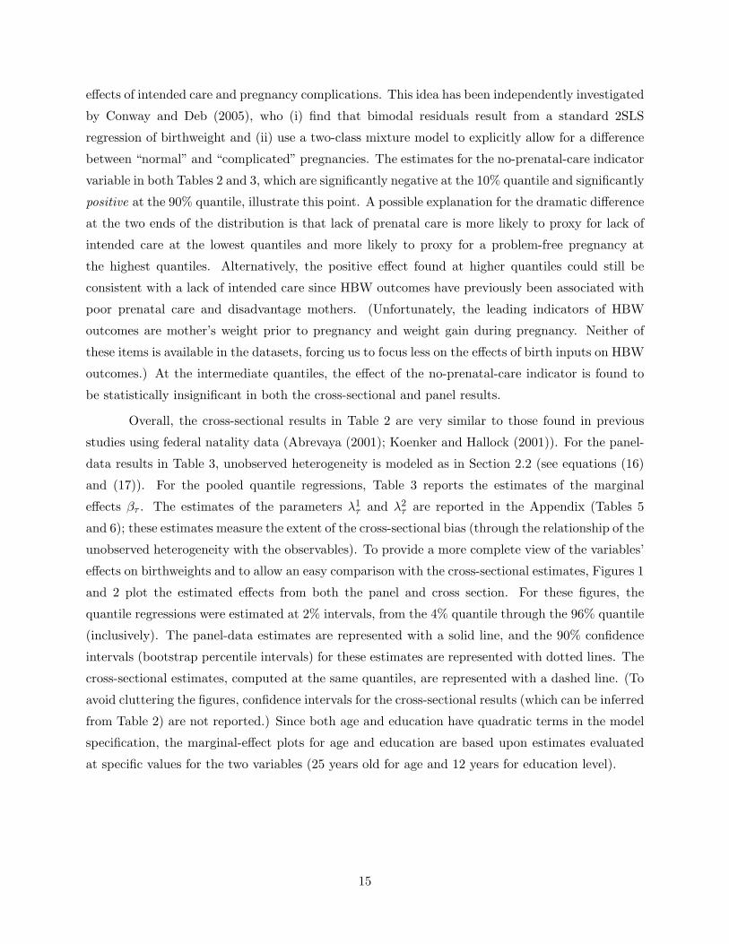
effects of intended care and pregnancy complications. This idea has been independently investigated
by Conway and Deb (2005), who (i) find that bimodal residuals result from a standard 2SLS
regression of birthweight and (ii) use a two-class mixture model to explicitly allow for a difference
between “normal” and “complicated” pregnancies. The estimates for the no-prenatal-care indicator
variable in both Tables 2 and 3, which are significantly negative at the 10% quantile and significantly
positive at the 90% quantile, illustrate this point. A possible explanation for the dramatic difference
at the two ends of the distribution is that lack of prenatal care is more likely to proxy for lack of
intended care at the lowest quantiles and more likely to proxy for a problem-free pregnancy at
the highest quantiles. Alternatively, the positive effect found at higher quantiles could still be
consistent with a lack of intended care since HBW outcomes have previously been associated with
poor prenatal care and disadvantage mothers. (Unfortunately, the leading indicators of HBW
outcomes are mother’s weight prior to pregnancy and weight gain during pregnancy. Neither of
these items is available in the datasets, forcing us to focus less on the effects of birth inputs on HBW
outcomes.) At the intermediate quantiles, the effect of the no-prenatal-care indicator is found to
be statistically insignificant in both the cross-sectional and panel results.
Overall, the cross-sectional results in Table 2 are very similar to those found in previous
studies using federal natality data (Abrevaya (2001); Koenker and Hallock (2001)). For the panel-
data results in Table 3, unobserved heterogeneity is modeled as in Section 2.2 (see equations (16)
and (17)). For the pooled quantile regressions, Table 3 reports the estimates of the marginal
effects βτ . The estimates of the parameters λ1τ and λ2
τ are reported in the Appendix (Tables 5
and 6); these estimates measure the extent of the cross-sectional bias (through the relationship of the
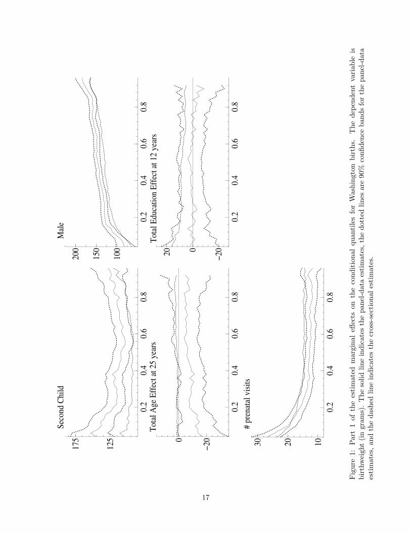
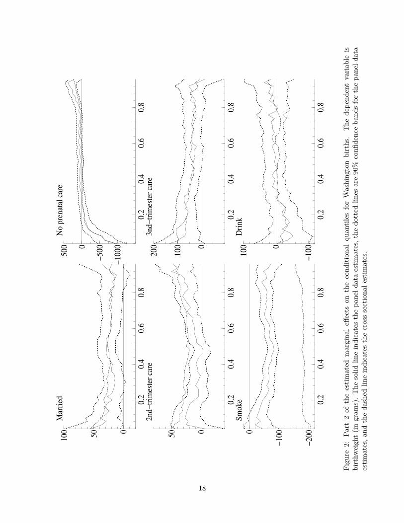
unobserved heterogeneity with the observables). To provide a more complete view of the variables’
effects on birthweights and to allow an easy comparison with the cross-sectional estimates, Figures 1
and 2 plot the estimated effects from both the panel and cross section. For these figures, the
quantile regressions were estimated at 2% intervals, from the 4% quantile through the 96% quantile
(inclusively). The panel-data estimates are represented with a solid line, and the 90% confidence
intervals (bootstrap percentile intervals) for these estimates are represented with dotted lines. The
cross-sectional estimates, computed at the same quantiles, are represented with a dashed line. (To
avoid cluttering the figures, confidence intervals for the cross-sectional results (which can be inferred
from Table 2) are not reported.) Since both age and education have quadratic terms in the model
specification, the marginal-effect plots for age and education are based upon estimates evaluated
at specific values for the two variables (25 years old for age and 12 years for education level).
15
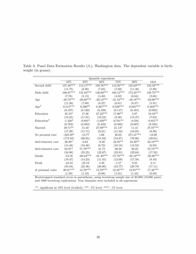
Table 3: Panel Data Estimation Results (βτ ), Washington data. The dependent variable is birth-weight (in grams).
Quantile regressions10% 25% 50% 75% 90% OLS
Second child 137.46*** 113.17*** 109.76*** 113.56*** 125.63*** 122.32***(11.75) (8.30) (7.03) (7.69) (11.38) (5.99)
Male child 100.67*** 131.64*** 146.69*** 160.12*** 173.35*** 138.75***(7.76) (5.15) (4.40) (4.82) (6.64) (3.68)
Age -38.73*** -20.88*** -30.13*** -31.52*** -48.18*** -33.06***(11.26) (7.00) (6.27) (6.61) (9.47) (5.31)
Age2 0.515*** 0.290** 0.467*** 0.529*** 0.845*** 0.483***(0.197) (0.120) (0.109) (0.117) (0.161) (0.092)
Education 35.54* 17.26 27.22*** 17.96** 5.97 19.16**(18.25) (11.91) (10.23) (8.46) (13.47) (7.62)
Education2 -1.436* -0.881* -1.029** -0.761** -0.594 -0.851**(0.762) (0.503) (0.433) (0.388) (0.607) (0.334)
Married 39.71** 15.49 27.99*** 21.13* 11.41 27.87***(17.26) (11.71) (9.21) (11.32) (16.05) (8.30)
No prenatal care -323.39* -13.77 1.66 26.03 271.21*** -18.08(172.94) (60.05) (51.94) (54.87) (76.06) (49.01)
2nd-trimester care 26.80* 6.63 -0.20 22.95** 34.39** 22.19***(14.48) (10.46) (8.72) (10.18) (13.52) (6.93)
3nd-trimester care 62.87* 71.79*** 31.75 30.50 39.22 55.73***(34.96) (25.25) (22.67) (23.91) (32.04) (17.32)
Smoke -24.58 -60.64*** -81.43*** -57.70*** -56.19*** -56.86***(19.47) (14.23) (11.45) (12.09) (17.58) (9.10)
Drink -44.24 -32.19 4.29 -1.57 9.25 2.11(35.84) (25.36) (20.00) (24.77) (29.79) (17.11)
# prenatal visits 20.01*** 14.79*** 12.70*** 12.32*** 12.65*** 17.48***(1.59) (1.10) (0.88) (1.01) (1.43) (0.93)
Bootstrapped standard errors in parentheses, using bootstrap sample size of 20,000 (10,000 pairs)and 1000 bootstrap replications. Year dummies were included in all regressions.
‘*’: significant at 10% level (2-sided); ‘**’: 5% level; ‘***’: 1% level.
16
0.2
0.4
0.6
0.8
125
175
Seco
nd C
hild
0.2
0.4
0.6
0.8
100
150
200
Mal
e
0.2
0.4
0.6
0.8
−200
Tota
l Age
Eff
ect a
t 25
year
s
0.2
0.4
0.6
0.8
−20020
Tota
l Edu
catio
n Ef
fect
at 1
2 ye
ars
0.2
0.4
0.6
0.8
102030#
pren
atal
vis
its
Fig
ure
1:Par
t1
ofth
ees
tim
ated
mar
gina
leff
ects
onth
eco
ndit
iona
lqu
anti
les
for
Was
hing
ton
birt
hs.
The
depe
nden
tva
riab
leis
birt
hwei
ght
(in
gram
s).
The
solid
line
indi
cate
sth
epa
nel-da
taes
tim
ates
,the
dott
edlin
esar
e90
%co
nfide
nce
band
sfo
rth
epa
nel-da
taes
tim
ates
,an
dth
eda
shed
line
indi
cate
sth
ecr
oss-
sect
iona
les
tim
ates
.
17
0.2
0.4
0.6
0.8
050100
Mar
ried
0.2
0.4
0.6
0.8
−100
0
−5000
500
No
pren
atal
car
e
0.2
0.4
0.6
0.8
050
2nd−
trim
este
r car
e
0.2
0.4
0.6
0.8
0
100
200
3nd−
trim
este
r car
e
0.2
0.4
0.6
0.8
−200
−1000
Smok
e
0.2
0.4
0.6
0.8
−1000
100
Drin
k
Fig
ure
2:Par
t2
ofth
ees
tim
ated
mar
gina
leff
ects
onth
eco
ndit
iona
lqu
anti
les
for
Was
hing
ton
birt
hs.
The
depe
nden
tva
riab
leis
birt
hwei
ght
(in
gram
s).
The
solid
line
indi
cate
sth
epa
nel-da
taes
tim
ates
,the
dott
edlin
esar
e90
%co
nfide
nce
band
sfo
rth
epa
nel-da
taes
tim
ates
,an
dth
eda
shed
line
indi
cate
sth
ecr
oss-
sect
iona
les
tim
ates
.
18

The estimated effects of the various variables, as presented in Tables 2 and 3 and Figures 1
and 2, are discussed in more detailed below:
Second child: Birthweights are uniformly larger for second children at all quantiles, for both
the cross-sectional and panel estimates. The panel estimates of the second-child effect are
somewhat larger than the cross-sectional estimates, with the largest effects at the lowest
quantiles (e.g., 137 grams at the 10% quantile).
Male child: It is well-known that, on average, male babies weigh more at birth than female babies.
The quantile estimates indicate that the positive male-child effect on birthweight is present at
all quantiles of the conditional birthweight distribution. The magnitude of the effect increases
when one moves from lower quantiles to higher quantiles, with the panel estimates indicating
a slightly higher effect (10–20 grams) than the cross-sectional estimates.
Age and education: Figure 1 shows the estimated (one-year) effects of age and education, evaluated
at 25 years of age and 12 years of education, respectively. For age, both the cross-sectional and
panel estimates are very close to zero in magnitude (and statistically insignificant at a 5% level
for all quantiles). For education, the cross-sectional estimates are positive across the quantiles
and statistically significant (at a 5% level) except at quantiles above 80%. In contrast, the
panel estimates are statistically insignificant across all quantiles. This difference could be due
to two factors: (i) the amount of within-mother variation in education is quite small, with
the average change in education for the sample being about 0.2 years; and, (ii) the level of
education may be related to the mother-specific unobservable. For the latter factor, years of
schooling is likely positively related to cm, which would imply an upward bias in the cross-
sectional estimates that is consistent with Figure 1. The issue of education being potentially
mismeasured is briefly discussed in Section 4.3.2. Results for other age and education levels
are reported in Abrevaya and Dahl (2006).
Marital status: The estimated positive effects of marriage on birthweight are quite similar for the
cross-sectional and panel specifications, in the 20–50 gram range over the quantiles considered.
One should be cautious about interpreting the cross-sectional marriage estimates as causal
since marital status is an explanatory variable that a priore would appear to serve as a proxy
for mother-specific unobservables (i.e., marital status positively correlated with cm). The
panel estimates are slightly lower than the cross-sectional estimates in the lower quantiles
(until around the 40% quantile), suggesting that this might be a factor in the lower quantiles.
Somewhat surprisingly, however, the panel estimates of the marriage effect remain positive
throughout the range of quantiles and significantly so (at the 10% level) at nearly all the
quantiles below 80%. On the whole, the estimates are consistent with a situation in which
19

marriage provides the birth mother with support (financial support, emotional support, etc.)
that would lead to a more favorable birth outcome.
Prenatal-care visits: Lack of prenatal care is found to have a significant negative effects at lower
quantiles and significant positive effects at the upper quantiles. The estimated effects are
similar for both the cross-sectional and panel regressions. As discussed above, a logical
explanation is that the “No prenatal care” indicator variable may proxy for poor care at lower
quantiles but for problem-free pregnancies at upper quantiles. For the third-trimester-care
indicator variable, the cross-sectional and panel estimates are also similar, indicating positive
effects (as compared to first-trimester care) which become less statistically significant at higher
quantiles. For the indicator variables, the largest difference between the cross-sectional and
panel results shows up in the second-trimester-care variable; the cross-sectional estimates are
statistically significant at all quantiles and range from 25 to 50 grams, whereas the panel
estimates are somewhat lower (close to zero in intermediate quantiles) and only significantly
positive at the highest quantiles. The effect of the number of prenatal visits is estimated to
be significantly positive across all quantiles, with larger effects found at lower quantiles and
the effects essentially “flattening out” (at around 14–15 grams per visit for the cross-sectional
results and 12–13 grams per visit for the panel results). The estimated effects for the panel
specification exhibit a sharper decline, leading to lower estimates (roughly a 2-gram per-visit
differential) than the cross-sectional specification. This variable shows up significantly in the
λ1τ and λ2
τ estimates (see Tables 5 and 6), leading to the differences found and suggesting that
the variable is related to the mother-specific unobservable.
Smoking: The most dramatic differences between the cross-sectional and panel results are the
estimated effects of smoking. The cross-sectional results indicate that the negative effects
of smoking are in the range of 150–200 grams, with larger effects at lower quantiles. The
panel estimates are still significantly negative at all but the lowest quantiles, but the esti-
mated effects are much lower in magnitude (mostly in the 50–80 gram range between the 20%
and 80% quantiles). The omitted-variables explanation of this large difference would be that
the smoking indicator in the cross-sectional specification is negatively related with the error
disturbance in the birthweight regression equation. Consistent with this explanation, the
smoking coefficients in both λ1τ and λ2
τ are found to be significantly negative across the quan-
tiles (Tables 5 and 6). The magnitudes of the panel estimates are also significantly lower than
those found in previous work, including quasi-experimental estimates based upon cigarette-
tax changes (e.g., Evans and Ringel (1999) and Lien and Evans (2005)) and experimental
estimates (e.g., Permutt and Hebel (1989)). These studies have estimated causal (IV) effects
of smoking on birthweight which are not statistically different from the OLS estimates; these
20
estimates have relatively large standard errors (due to the sources of variation exploited) and,
in some cases, are even larger in magnitude than the OLS estimates. We believe that our
panel estimates are quite credible given the compelling nature of the omitted-variables expla-
nation in this context. We note, however, that our results do not directly contradict those
found by instrumental-variables methods. First, the IV estimates are quite imprecise (large
standard errors), so our estimates would also fall within reasonable confidence intervals for
these previous studies. Second, the panel estimates are identified from mothers who change
their smoking status for any reason whereas the IV estimates are identified from mothers
who change their smoking status in response to a specific treatment (e.g., prenatal counseling
or cigarette-tax increases); since these subpopulations are different, the underlying treatment
effects could themselves also be different. Finally, we point out that misclassification of smok-
ing status could explain part of the difference found here since the effect of misclassification is
more severe in the panel-data case (see, for example, Freeman (1984) and Jakubson (1986)).
This possibility is further discussed in Section 4.3.2.
Alcohol consumption: In contrast to the smoking results, the estimated effects of alcohol consump-
tion are quite similar for the cross-sectional and panel specifications. Drinking is estimated
to have significant negative effects at lower quantiles (below about the 20% quantile), with
the magnitudes of the effects ranging between about 40 and 80 grams. Of course, very few
mothers actually report alcohol consumption during pregnancy (only about 1.5% in our sam-
ple). The lack of strong statistical evidence regarding the effects of drinking could stem from
the low variation in the indicator variable and the probable large rates of misclassification.
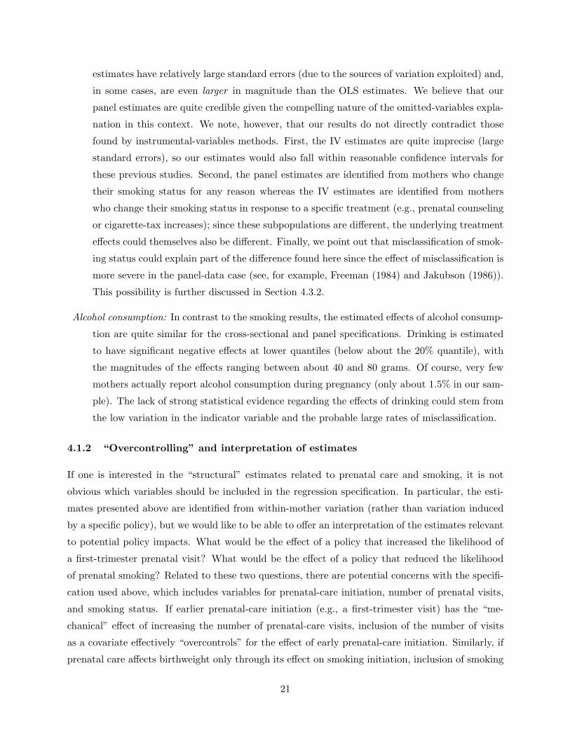
4.1.2 “Overcontrolling” and interpretation of estimates
If one is interested in the “structural” estimates related to prenatal care and smoking, it is not
obvious which variables should be included in the regression specification. In particular, the esti-
mates presented above are identified from within-mother variation (rather than variation induced
by a specific policy), but we would like to be able to offer an interpretation of the estimates relevant
to potential policy impacts. What would be the effect of a policy that increased the likelihood of
a first-trimester prenatal visit? What would be the effect of a policy that reduced the likelihood
of prenatal smoking? Related to these two questions, there are potential concerns with the specifi-
cation used above, which includes variables for prenatal-care initiation, number of prenatal visits,
and smoking status. If earlier prenatal-care initiation (e.g., a first-trimester visit) has the “me-
chanical” effect of increasing the number of prenatal-care visits, inclusion of the number of visits
as a covariate effectively “overcontrols” for the effect of early prenatal-care initiation. Similarly, if
prenatal care affects birthweight only through its effect on smoking initiation, inclusion of smoking
21
0.1 0.2 0.3 0.4 0.5 0.6 0.7 0.8 0.9
−1000
−500
0
500 No prenatal care
0.1 0.2 0.3 0.4 0.5 0.6 0.7 0.8 0.9
−50
0
50 2nd−trimester care
0.1 0.2 0.3 0.4 0.5 0.6 0.7 0.8 0.9
0
100 3nd−trimester care
Figure 3: Results for initial-prenatal-visit variables under different specifications (Washingtondata). The solid line corresponds to the full specification, the dotted line to the specificationin which “# of prenatal visits” is dropped, and the dashed line to the specification in which “# ofprenatal visits,” “Smoke,” and “Drink” are dropped. The omitted category is first-trimester care.
status as a covariate could also be an “overcontrolling” factor.
To empirically assess the possible importance of “overcontrolling,” we re-ran the Washington
regressions under two alternative specifications: (i) original specification with number of prenatal
visits dropped, and (ii) original specification with number of prenatal visits, smoking status, and
drinking status dropped. Figure 3 reports the estimates on the prenatal-care-initiation categorical
variables for these two specifications along with the original specification. Dropping the number of
prenatal visits from the specification has important consequences. For each of the three variables
(which are interpreted as differences from first-trimester care), there is a significant drop in the
coefficient estimates across the quantiles. The second-trimester estimate goes from being positive
(and statistically insignificant) at most quantiles to being negative and statistically significant (at
a 10% level) at all quantiles below 60%. The no-prenatal-care variable also becomes negative
and statistically significant (at a 10% level) at all quantiles below 60%. (Note the difference
in scale on the y axes for the three variables.) The third-trimester estimate goes from being
significantly positive at most quantiles to being negative, but statistically insignificant, at most
quantiles. Overall, if one views first-trimester prenatal care as mechanically increasing the number
of prenatal-care visits, the estimates from Figure 3 indicate that the structural effect of increasing
early prenatal-care initiation would be to increase birthweight at lower quantiles (with small effects
22

of about 20 grams for transitions from second-trimester care to first-trimester care and much larger
effects for transitions from no prenatal care to first-trimester care). We also note that the estimates
on the other variables (those not shown in Figure 3) remain essentially unchanged when number
of visits is dropped from the specification.
When smoking status and drinking status are also dropped from the specification, there is
essentially no change in the prenatal-care-initiation estimates shown in Figure 3 (the comparison
between the dotted and dashed lines). This suggests that the inclusion of smoking status in the
original specification (and also in the one dropping number of visits) did not have an impact on
the estimated effect of the timing of prenatal-care initiation. Alternatively, in thinking of other
variables as possibly “overcontrolling” for smoking status, we tried several specifications in which
other covariates were dropped from specifications in which smoking status remained. For these
specifications, we found estimated smoking effects that were extremely similar to those reported in
Figure 1. These results make us more comfortable about interpreting the original smoking estimates
(Figure 1) as structural effects upon the conditional quantile distribution.
4.1.3 Arizona data
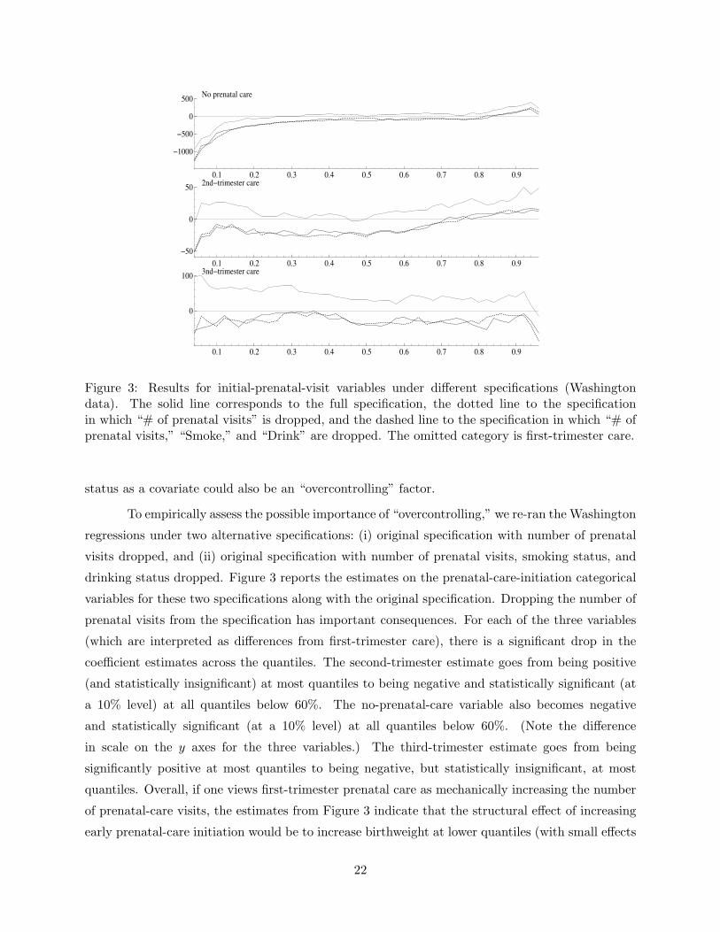
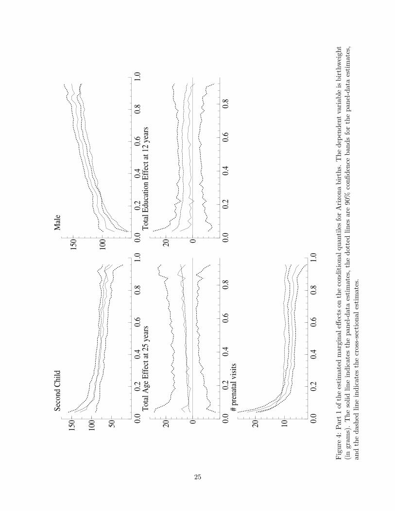
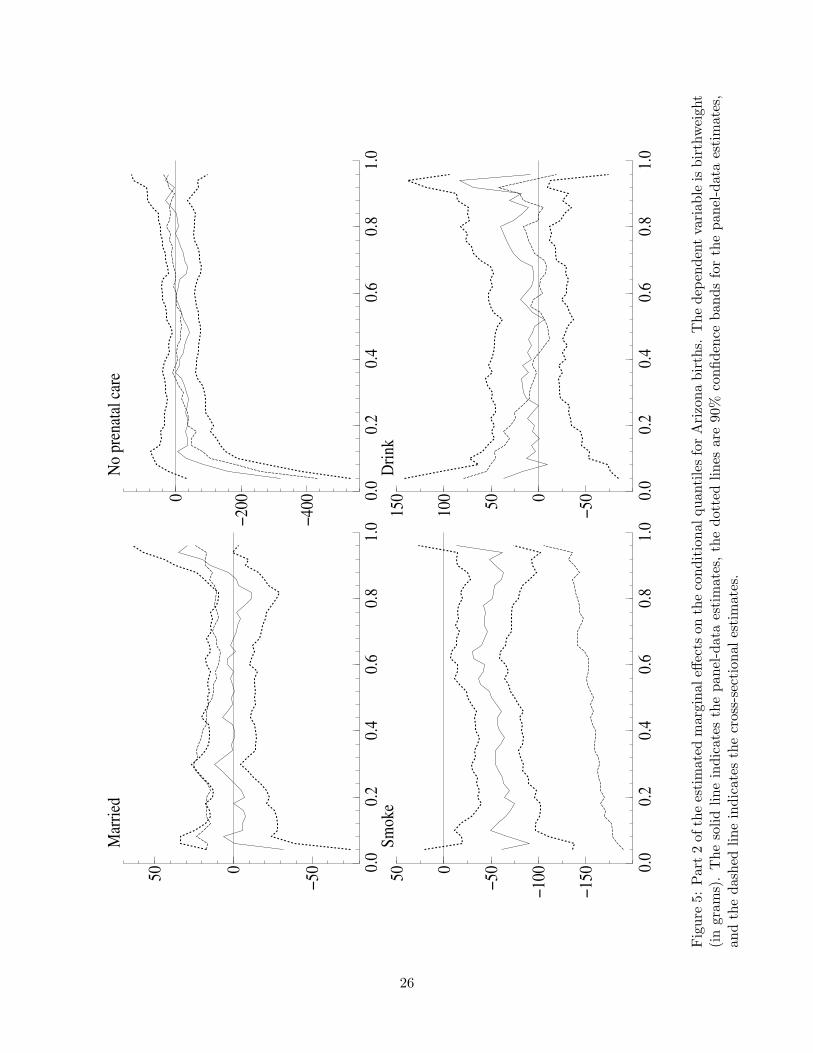
Figures 4 and 5 plot the estimated quantile effects (4% through 96% quantiles, inclusively) for the
Arizona maternally-linked sample. The same model specification discussed above was used, except
that indicator variables for second-trimester and third-trimester prenatal care were not included.
The figures are comparable to Figures 1 and 2 for the Washington data, with the age effect reported
at 25 years and the education effect at 12 years.
Overall, there is a remarkable similarity between the results for the two samples. The
common findings for the two samples include the following:
• There is a significant positive effect of the second child across all quantiles (50–125 grams in
the Arizona panel estimates).
• The positive birthweight effect of a male child increases from lower to higher quantiles.
• Despite a positive estimated cross-sectional effect of education at lower quantiles, the panel
estimates indicate no significant education effect.
• The effect of the number of prenatal visits is highest at lower quantiles, with the effect
flattening out at higher quantiles. For both Washington and Arizona, the cross-sectional
estimate of the effect is lower at lower quantiles and higher at higher quantiles.
• The magnitude of the negative smoking effect is significantly lower for the panel estimates
(ranging between 40 and 80 grams for Arizona) than for the cross-sectional estimates.
23

Some differences between the results for the two samples are also worth noting:
• Although the cross-sectional estimates of the marriage effect are still significantly positive (p-
values lower than 0.10 throughout the range of quantiles), the panel-data estimates indicate
no statistically significant effect of marriage for Arizona mothers. The likely explanation
of this finding is that the father’s date of birth is required to match for both births of an
Arizona mother (see Section 3), meaning that the father is the same even if marital status
differs across the births. For the Washington sample, a change in marital status might also
be related to a change in father.
• Due to the lack of indicator variables for second-trimester and third-trimester care, the esti-
mated effects of the no-care indicator variable and the number of prenatal visits are slightly
different. The magnitude of the quantile effects for number of prenatal visits is roughly 50%
lower for the Arizona sample, although the shape of the quantile-effect curve is extremely
similar. The shape of the no-prenatal-care effect is also very similar to that of Washington,
but the estimated panel effects are not significantly different from zero at any of the quantiles.
24
0.0
0.2
0.4
0.6
0.8
1.0
50100
150
Seco
nd C
hild
0.0
0.2
0.4
0.6
0.8
1.0
100
150
Mal
e
0.0
0.2
0.4
0.6
0.8
020
Tota
l Age
Eff
ect a
t 25
year
s
0.0
0.2
0.4
0.6
0.8
020
Tota
l Edu
catio
n Ef
fect
at 1
2 ye
ars
0.0
0.2
0.4
0.6
0.8
1.0
1020
# pr
enat
al v
isits
Fig
ure
4:Par
t1
ofth
ees
tim
ated
mar
gina
leffe
cts
onth
eco
ndit
iona
lqua
ntile
sfo
rA
rizo
nabi
rths
.T
hede
pend
ent
vari
able
isbi
rthw
eigh
t(i
ngr
ams)
.T
heso
lidlin
ein
dica
tes
the
pane
l-da
taes
tim
ates
,th
edo
tted
lines
are
90%
confi
denc
eba
nds
for
the
pane
l-da
taes
tim
ates
,an
dth
eda
shed
line
indi
cate
sth
ecr
oss-
sect
iona
les
tim
ates
.
25
0.0
0.2
0.4
0.6
0.8
1.0
−50050
Mar
ried
0.0
0.2
0.4
0.6
0.8
1.0
−400
−2000
No
pren
atal
car
e
0.0
0.2
0.4
0.6
0.8
1.0
−150
−100−5
0050Sm
oke
0.0
0.2
0.4
0.6
0.8
1.0
−50050100
150
Drin
k
Fig
ure
5:Par
t2
ofth
ees
tim
ated
mar
gina
leffe
cts
onth
eco
ndit
iona
lqua
ntile
sfo
rA
rizo
nabi
rths
.T
hede
pend
ent
vari
able
isbi
rthw
eigh
t(i
ngr
ams)
.T
heso
lidlin
ein
dica
tes
the
pane
l-da
taes
tim
ates
,th
edo
tted
lines
are
90%
confi
denc
eba
nds
for
the
pane
l-da
taes
tim
ates
,an
dth
eda
shed
line
indi
cate
sth
ecr
oss-
sect
iona
les
tim
ates
.
26

4.2 Hypothesis testing
In this section, we discuss the results of several hypothesis tests that were used in order to test the
model specification and/or the significance of differences across the estimates at different quantiles.
The minimum-distance (MD) framework of Buchinsky (1998) is used (and extended to the panel-
data case) to test various (linear) restrictions placed on the parameters in the estimated models.
4.2.1 Minimum-distance testing framework
Let p denote the number of different quantiles at which the model is estimated, with τ1, . . . , τp
denoting the quantiles. For a given quantile τ , individual elements of the parameter vectors β, λ1τ ,
and λ2τ (recall the model in (16) and (17)) are referenced by subscripts as follows:
βτ = (βτ1, ..., βτL)′ , λ1τ =
(λ1
τ1, . . . , λ1τK
)′, λ2
τ =(λ2
τ1, . . . , λ2τK
)′,
where K is the number of variables in xm1 and xm2. For generality, βτ has L ≥ K elements, to allow
for additional variables (e.g., time-invariant regressors) that may not appear in the λ estimates.
Then, for a given quantile τ , the full parameter vector is denoted
γτ ≡(φ1
τ , βτ0, β′τ , λ
1τ′, λ2
τ′)′, (19)
where βτ0 ≡ φ2τ − φ1
τ . The (stacked) parameter vector for all of the estimated quantiles is denoted
γ ≡ (γ′τ1 , γ
′τ2 , . . . , γ
′τp
)′ (20)
and has dimension p(2K +L+ 2) × 1. Further, let γ denote the estimator of γ, and define A to be
the estimated variance-covariance matrix (obtained via the bootstrap) of γ.
In the MD framework, the “restricted” parameter estimator is defined as
γR = arg minγR∈Θ
(γ −RγR
)′A−1 (
γ −RγR), (21)
where R is a restriction matrix that will depend on the type of restrictions imposed. Since only
linear restrictions are considered, γR can be written explicitly as
γR =(R′A−1R
)−1 (R′A−1γ
). (22)
The asymptotic variance of γR is given by
var(γR) =(R′A−1R
)−1. (23)
For the purposes of hypothesis testing, note that under the null hypothesis that the restrictions are
true (i.e., H0 : γ = RγR), the following MD test statistic has a limiting chi-square distribution:(γ −RγR
)′A−1 (
γ −RγR) d−→
H0χ2
M , (24)
27

where M is the number of restrictions (i.e., M = rows (R)−columns (R)). The Appendix provides
specific details on the appropriate choice of R and M for each of the tests described below.
4.2.2 Test results
Using the MD testing framework, the following hypothesis tests were conducted:
Test of correlated random effects: To determine whether a “pure” random effects specification
(in which cm is uncorrelated with xm) would be rejected for a given quantile τ , the null
hypothesis H0 : λ1τ = λ2
τ = 0 is tested. For the quantiles τ ∈ {0.10, 0.25, 0.50, 0.75, 0.90}, the
null hypothesis is overwhelmingly rejected with p-values extremely close to zero.
Test of the equality of the “effect vector” across quantiles: This test considers whether there are any
statistically significant differences in the βτ estimates across two different quantiles. For the
panel specifications, we conducted this test for each pairwise combination of quantiles from
the set {0.10, 0.25, 0.50, 0.75, 0.90}. For Washington, the p-values (all below 2%) indicate
very significant differences across the quantiles. For Arizona, there are significant differences
between the lowest quantiles (10% and 25%) and other quantiles; however, the p-values for the
50%/90% and the 75%/90% comparisons do not indicate a statistically significant difference
in the βτ estimates.
Test of the equality of individual variables’ effects across quantiles: For a given variable (for
example, marital status), this test checks whether the estimated effects at different quantiles
are significantly different. The set of different quantiles considered is the same as that used
in Tables 2–3. For the marriage indicator, for instance, the null hypothesis would be H0 :
βmarriedτ=0.10 = βmarried
τ=0.25 = βmarriedτ=0.50 = βmarried
τ=0.75 = βmarriedτ=0.90 . Since both age and education enter
into the model specification in two terms (a linear term and a quadratic term), the appropriate
tests for these two variables are joint tests of equality. The test results (p-values) for all of
the variables, in both the cross-sectional and panel specifications, are reported in Table 4
for Washington and Arizona. The results are very much in line with the quantile-estimate
graphs in Figures 1–2 and Figures 4–5. Two variables (male-child indicator and number of
prenatal visits) vary significantly across the quantiles for both the cross-sectional and panel
specifications. The effect of the no-prenatal-care indicator also varies significantly (p-value
of 0.010 in the cross section and 0.004 in the panel) for the Washington sample. On the
other hand, there is no statistical evidence that the effects of marital status or drinking
vary over quantiles in either specification. The cross-sectional estimated effects of both age
and education vary significantly across quantiles, whereas the panel estimated effects do not.
For the smoking-indicator variable, the p-value for the Washington cross-sectional results is
28

Table 4: Tests of Marginal-Effect Equality Across Quantiles. For each covariate, p-values basedupon cross-sectional and panel-data estimates are reported for the null hypothesis of equality ofmarginal effects for the five quantiles 0.10, 0.25, 0.50, 0.75, and 0.90. Results are based upon 1,000bootstrap replications.
Washington ArizonaCross Panel Cross Panel
Section Data Section DataSecond child 0.135 0.113 0.000 0.049Male child 0.000 0.000 0.000 0.000Age, age2 jointly 0.006 0.088 0.000 0.944Education, education2 jointly 0.014 0.336 0.002 0.927Married 0.574 0.457 0.565 0.739No prenatal care 0.010 0.004 0.442 0.8742nd-trimester care 0.620 0.059 — —3nd-trimester care 0.154 0.638 — —Smoke 0.257 0.063 0.236 0.834Drink 0.578 0.602 0.346 0.905# prenatal visits 0.005 0.000 0.005 0.000
quite high (0.396), whereas the p-value (0.063) for the panel specification suggests a more
significant difference in the estimated effects across quantiles. Finally, it should be noted that
the choice of the quantile set {0.10, 0.25, 0.50, 0.75, 0.90} is admittedly arbitrary, following
what has become the convention for quantile regression.
4.3 Endogeneity Issues
In this section, we consider the sensitivity of the estimation results to possible sources of endogene-
ity. Note that the estimation method introduced in Section 2 (and discussed further in Section 5)
is based upon the assumption of strict exogeneity and, in general, will be inconsistent when this
assumption is violated. The two most important sources of endogeneity in the current application
are: (1) a “feedback effect” by which the first-birth outcome (birthweight) influences second-birth
explanatory variables (e.g., a low-birthweight first-birth outcome causing a mother to quit smoking
for the second birth) and (2) mismeasured explanatory variables.
4.3.1 Feedback or dynamic effects
The issue of feedback effects is discussed at length in Abrevaya (2006) in the context of a conditional-
expectation model, where instrumental-variables methods (using lagged birthweights as instru-
ments) can be utilized. Unfortunately, there is no obvious analogue to instrumental variables in
29
the conditional-quantile context. Instead, to see if allowing for dynamic effects alters the panel-data
estimates in an important way, we consider an augmented model specification in which lagged birth-
weight is included as an explanatory variable. Specifically, since data on two births per mother are
available, ym1 (first-birth birthweight) is included as a right-hand-side variable for the second-birth
equation. (Considering matched panel data with three births per mother reduces the sample size
to an extent which makes all of the estimates imprecise.) Only a single coefficient for ym1 in the
second-birth equation can be estimated; there is no way to separately identify coefficients within
both βτ and λ2τ .
Overall, the inclusion of lagged birthweight in the second-birth equation does not have a
large effect on the estimated effects of the other observable variables. Lagged birthweight is found
to be a significant predictor of second-birth birthweight, with coefficient estimates around 0.45 at
the lower quantiles and gradually decreasing to around 0.40 at the higher quantiles. Despite the
significant effects of lagged birthweight, the estimated effects of smoking do not change much. The
new estimates are mostly flat at around −75 grams, just slightly below the original panel estimates.
The interested reader is referred to Abrevaya and Dahl (2006) for more details.
Another source of endogeneity related to “feedback effects” is that the decision to have
a second child may itself be affected by the first-birth outcome. For instance, one might expect
mothers with a particularly adverse (good) first-birth outcome to be less (more) likely to have a
second child. This source of endogeneity is difficult to handle without more a more explicit model of
the second-birth selection/attrition process, and the present data do not provide obvious candidates
for convincing exclusion restrictions in such a model.
4.3.2 Measurement error
To examine the issue of measurement error, we focus on two explanatory variables: education and
smoking. Since the panel-data estimated effects of education are insignificant, it is worthwhile
to examine whether measurement error in education might be causing an attenuation bias in the
estimated effects. For smoking, the panel-data approach yields vastly different estimates (lower in
magnitude) than the cross-sectional approach. As discussed in Section 4.1.1, one possible cause of
these lower magnitudes is misclassification of smoking status (specifically, smokers being misclassi-
fied as non-smokers). Freeman (1984) and Jakubson (1986) have shown that the attenuation bias
from misclassification of an explanatory variable can be more severe in the panel-data case than
the cross-sectional case. Unfortunately, cross-validation data are not available for the education
and smoking variables.
For education, there are cross-sectional units for which the education variable must be
mismeasured due to inconsistencies in reporting from the first-birth data to the second-birth data.
30
Using the Washington data, we dropped all observations having (i) more additional education than
possible given the change in age (ΔEducation > ΔAge + 1) or (ii) a drop in years of education
(ΔEducation < 0). There were 5,455 mothers (12% of the sample) with such inconsistencies in
reported education, with 346 mothers in group (i), 5,117 in group (ii), and 8 in both. Re-running
the panel-data regressions on the less error-ridden subsample yielded extremely similar results to
the original regressions, with the education effects remaining insignificant and the other estimated
effects being nearly identical. More details are provided in Abrevaya and Dahl (2006). Of course,
there may be other forms of reporting errors in education (see, for example, Kane, Rouse, and
Staiger (1999)), but cross-validation data would be required to examine these.
To gauge the sensitivity of the smoking-effect estimates to possible misclassification of smok-
ing status, we conducted simulations where we artificially introduced misclassification into the esti-
mation sample. In each simulation, we misclassified a fraction q (for q = 0.1 and q = 0.2) of observed
smokers as non-smokers and then compute the panel-data estimates (at τ ∈ {0.1, 0.2, . . . , 0.8, 0.9}.
(We assume no misclassification of non-smokers as smokers.) Abrevaya and Dahl (2006) report
details of the simulation results, which we briefly summarize here. As expected, the artificial mis-
classification induces an attenuation bias in the estimated smoking effect. The simulations suggest
biases on the order of 20–80% for the misclassification rates considered, biases which are far too
small to explain the difference between the cross-sectional and panel estimates. For 20% misclassi-
fication, the simulations suggest that misclassification bias accounts for nearly half of the difference
between the panel and cross-sectional estimates; however, at quantiles away from the median (es-
pecially so at the 10% quantile), the misclassification bias accounts for less of the difference from
the cross-sectional estimates. Finally, we note that the “model” of misclassification used to create
the artificial datasets is too simplistic since it does not allow for (i) a mother’s reporting errors to
be correlated over time or (ii) reporting errors to be correlated with other observables. The first
issue is considered by Abrevaya (2006), where it is shown that positive correlation in misreporting
(i.e., a mother who misreports during her first pregnancy is more likely to misreport during her
second pregnancy) reduces the extent of the misclassification bias. The second issue is considerably
more difficult to analyze without some type of cross-validation data.
5 Discussion of the theoretical model
In this section, we provide a more formal discussion of the panel-data framework introduced in Sec-
tion 2. In doing so, we highlight the pros and cons of the proposed approach and suggest directions
for future research. To be consistent with the standard panel-data notation, this section will use i
(rather than m) to denote cross-sectional units and t (rather than b) to denote time. The number of
31

time periods T ≥ 2 for each cross-sectional unit is assumed to be fixed, whereas the number of cross-
sectional units n → ∞. The random variables {(xi1, . . . , xiT , ui1, . . . , uiT , ci)}ni=1 are assumed to be
i.i.d. draws from their underlying distributions. The observed data are {(yi1, . . . , yiT , xi1, . . . , xiT )}ni=1,
where each yit is generated according to the model
yit = x′itβ + ci + uit. (25)
The relationship between ci and xi ≡ (xi1, . . . , xiT ) is described by
ci = φ(xi) + vi, where E(vi|xi) = 0. (26)
Equation (26) is not restrictive, in the sense that the conditional-mean “assumption” (E(vi|xi) = 0)
is merely a normalization that fixes location.
For any τ ∈ (0, 1), the conditional τ -th quantile of yit is
Qτ (yit|xi) = x′itβ + φ(xi) +Qτ (vi + uit|xi). (27)
The assumptions related to the last term in (27), Qτ (vi + uit|xi), dictate how the marginal effects
of xit upon Qτ (yit|xi) can be identified. Consider the following two simplifying assumptions:
(B1) vi is independent of xi (28)
(B2) Qτ (uit|xi, vi) = Qτ (uit|xit). (29)
Assumption (B1) is commonly used in estimation of non-linear panel-data models with correlated
random effects. The data-generating process allows xi to affect the level of the yit variables (through
the φ(xi) function), but Assumption (B1) restricts the quantiles of the fixed effect to not depend
upon xi. Assumption (B2), which says that the quantiles of uit depend upon xi only through xit,
allows for arbitrary forms of xit-related heteroskedasticity. Note that Assumption (B2) also imposes
a form of strict exogeneity since the presence of feedback effects (relationships between past u’s
and future x’s) or lagged dependent variables would violate this assumption.
Taken together, Assumptions (B1) and (B2) imply that
Qτ (vi + uit|xi) = Qτ (vi + uit|xit) ≡ fτ,t(xit). (30)
The t subscript in fτ,t(xit) allows the relationship between the uit distribution and xit to change
with t. (If this relationship is assumed to be the same over time, the t subscript could be omitted,
leaving fτ (xit).) Plugging equation (30) into equation (27) yields
Qτ (yit|xi) = x′itβ + fτ,t(xit) + φ(xi). (31)
32
In general, both fτ,t and φ(xi) will be non-linear functions. Consider the following simple example,
which illustrates the inherent non-linearity of fτ,t:
Example: Linear-scale heteroskedasticity
The following distributional assumptions for ci and uit are made:
ci|xi ∼ N(ψ + x′i1λ1 + · · · + x′
itλT , σ2c )
uit|ci, xi ∼ N(0, (x′itγt)2)
These assumptions generalize the linear-scale model considered by Koenker and Bassett (1982) to
a panel-data setting and also impose normality. The variance of (ci + uit)|xi is σ2c + (x′
itγt)2, which
implies fτ,t(xit) = zτ√σ2
c + (x′itγt)2, where zτ denotes the τ -th quantile of the standard normal
distribution. In this example, linearity of fτ,t with respect to xit would only arise when σ2c = 0.
In the context of the general model described above (with Assumptions (B1) and (B2)),
the estimation approach proposed in Section 2 uses linear approximations for the two components
(x′itβ + fτ,t(xit) and φ(xi)) of the conditional quantile in equation (31). Specifically, generalizing
the notation used in Section 2 to T ≥ 2, x′itβτ is used to approximate x′
itβ + fτ,t(xit), and ψtτ +
x′i1λ
1τ +· · ·+x′
iTλTτ is used to approximate φ(xi). The conditional-quantile function in equation (31)
is additively separable in the functions of xit and xi, with φ(xi) entering the conditional-quantile
function in the same way in each time period. This separability makes it possible to directly estimate
the marginal effects of interest (i.e., the effects of xit upon x′itβ+fτ,t(xit)) by the proposed approach.
The most important topic for future research is to consider the situation in which Assump-
tion (B1) is violated. If the quantiles of vi depend upon xi, the conditional quantiles of yit will
not have the additive-separability property seen above. Instead, the conditional quantile function
would be a nonseparable function of xit and xi, say Qτ (yit|xi) = fτ,t(xit, xi). The effect of interest
is the derivative of fτ,t with respect to its first argument, where integration over the distribution
of xi could provide some type of average effect. A nonparametric approach to this problem, along
the lines of Altonji and Matzkin (2005), may be feasible. Alternatively, a linear-index approach (to
simplify how xit and/or xi enter into fτ,t) may prove useful. Another important topic for future
research is relaxation of strict exogeneity. Violations of strict exogeneity have been considered
extensively in the conditional-expecation panel-data models. For linear panel-data models, instru-
mental variables estimation is the usual solution to violations of the strict exogeneity assumption,
but such an approach is not likely to carry over to conditional-quantile models.
33
Acknowledgments
An earlier version of this paper circulated under the title, “The effects of smoking and prenatal
care on birth outcomes: evidence from quantile estimation on panel data.” Bill O’Brien, Patricia
Starzyk, and Dr. Beth Mueller offered invaluable assistance in providing access to the Washington
State Longitudinal Birth Database. The authors are also grateful to Christopher Mrela of the
Arizona Department of Health Services for providing birth data. The terms of the data-sharing
agreements with these two states do not allow release of this data. The authors would also like
to thank Roger Koenker and Daniel Morillo, who wrote the RQ 1.0 package for Ox that was
used as the starting point for the quantile estimation in this paper. An Associate Editor and two
referees provided extremely useful comments that vastly improved this paper. The first author
acknowledges financial support from a Kinley Trust Grant (Purdue University), the Robert Wood
Johnson Foundation, and the National Science Foundation (SES-0451660). The second author
acknowledges financial support from the Danish National Research Foundation and the Danish
Social Sciences Research Council (grant 275-06-0105).
Appendix A: Details on hypothesis testing
This section of the Appendix provides details on the hypothesis tests conducted in Section 4.2.2.
• (Test of correlated random effects) Test of H0 : λ1τi = 0 ∧ λ2
τi = 0 simultaneously ∀i ∈{1, . . . ,K} and ∀τ ∈ {τ1, τ2, . . . , τp}. Define
R′p(L+1)×p(2K+L+2)
≡[
Ip×p ⊗ [1 O1×(2K+L+1)
]Ip×p ⊗ [
O(L+1)×1 I(L+1)×(L+1) O(L+1)×2K
] ],
and use M = 2pK.
• (Test of the equality of the “effect vector”) Test of H0 : βτ1i = βτ2i = · · · = βτpi simultaneously
for ∀i ∈ {0, 1, 2, . . . , L}. Let ip be a (p, 1) vector of ones. To perform this test, define
R′ ≡⎡⎣ Ip×p ⊗ [
1 O1×((L+1)+2K)]
Ip×p ⊗ [O2K×(L+2) I2K×2K
]i′p ⊗ [
O(L+1)×1 I(L+1)×(L+1) O(L+1)×2K
]⎤⎦
and use M = (p− 1)(L+ 1).
• (Test of the equality of individual variables’ effects (single parameter)) Test of H0 : βτ1i =
βτ2i = · · · = βτpi for a single i ∈ {0, 1, 2, . . . , L}. Let
E1 ≡ Ip×p ⊗ [1 O1×((L+1)+2K)
],
E2 ≡ Ip×p ⊗ [O2K×(L+2) I2K×2K
],
E3 ≡ i′p−1 ⊗ [O(L+1)×1 Dii,(L+1)×(L+1) O(L+1)×2K
],
34

and
E4 ≡[
O(L+1)×1 I(L+1)×(L+1) O(L+1)×2K E3O(p−1)L×1 O(p−1)L×(L+1) O(p−1)L×2K I(p−1)×(p−1) ⊗ S−i·
],
where
S ≡ [O(L+1)×1 I(L+1)×(L+1) O(L+1)×2K
],
and S−i· is equal to S without the i’th row. Dii,(L+1)×(L+1) is a matrix of zeros except
for the entry (i, i) which equals unity. Then, the test of H0 can be performed by defining
R ≡ (E′1, E
′2, E
′4)
′, with M = p− 1.
• (Test of the equality of individual variables’ effects (joint test of two parameters)) Test of
H0 : βτ1i = βτ2i = · · · = βτpi ∧βτ1j = βτ2j = · · · = βτpj for i, j ∈ {0, 1, 2, . . . , L} and i �= j. Let
E1 ≡ Ip×p ⊗ [1 O1×((L+1)+2K)
],
E2 ≡ Ip×p ⊗ [O2K×(L+2) I2K×2K
],
E3 ≡ i′p−1 ⊗ [O(L+1)×1 D(ii,jj)(L+1)×(L+1) O(L+1)×2K
],
and
E4 ≡[
O(L+1)×1 I(L+1)×(L+1) O(L+1)×2K E3O(p−1)(L−1)×1 O(p−1)(L−1)×(L+1) O(p−1)(L−1)×2K I(p−1)×(p−1) ⊗ S−ij·
],
where
S ≡ [O(L+1)×1 I(L+1)×(L+1) O(L+1)×2K
],
and S−ij· is equal to S without rows i and j. D(ii,jj)(L+1)×(L+1) is a matrix of zeros except
for the entries (i, i) and (j, j) which both equal unity. To test H0, define R ≡ (E′1, E
′2, E
′4)
′
and use M = 2(p− 1).
Appendix B: Additional results
This section of the Appendix contains the Washington results for the estimates of λ1τ and λ2
τ (for
τ ∈ {0.10, 0.25, 0.50, 0.75, 0.90}) in Tables 5 and 6, respectively.
References
Abadie, Alberto, Joshua D. Angrist, and Guido Imbens, 2002, Instrumental variables estimates of
the effect of subsidized training on the quantiles of trainee earnings, Econometrica 70, 91–117.
Abrevaya, Jason, 2001, The effects of demographics and maternal behavior on the distribution of
birth outcomes, Empirical Economics, 26: 247–257.
35

Table 5: Panel-Data Estimation Results for λ1τ , Washington Data. The dependent variable is
birthweight (in grams). The coefficients represent the relationship between the covariates and thefirst-birth component of the correlated random effect.
Quantile regressions10% 25% 50% 75% 90% OLS
Male child -30.70*** -28.68*** -25.51*** -24.21*** -18.24** -23.95***(7.66) (5.47) (4.88) (5.61) (7.30) (4.50)
Age -4.50 -15.19 -4.64 -1.27 6.72 -8.29(14.77) (9.42) (8.98) (9.23) (12.06) (8.37)
Age2 0.222 0.341* 0.151 0.017 -0.153 0.224(0.277) (0.180) (0.174) (0.180) (0.231) (0.160)
Education -13.98 11.77 8.73 14.02* 26.44** 11.72(15.75) (11.43) (11.39) (8.51) (11.75) (8.58)
Education2 0.613 -0.290 -0.321 -0.464 -0.811 -0.360(0.672) (0.467) (0.460) (0.380) (0.534) (0.363)
Married -7.62 4.09 -7.19 -3.28 -2.29 -6.32(15.06) (9.89) (8.65) (10.02) (13.90) (8.27)
No prenatal care 103.15 97.91** 40.78 52.16 -71.85 34.70(86.87) (46.97) (45.18) (47.98) (54.24) (39.72)
2nd-trimester care 23.91 25.88** 30.29*** 12.18 15.69 20.56**(14.63) (10.54) (8.66) (9.91) (12.98) (8.43)
3nd-trimester care 69.72** 20.88 20.51 24.55 -0.73 31.31(29.96) (23.28) (22.15) (25.24) (33.56) (19.93)
Smoke -101.93*** -61.35*** -52.67*** -74.32*** -69.53*** -70.28***(16.34) (12.88) (10.23) (11.43) (14.73) (9.62)
Drink 0.07 -3.04 -26.93 -15.49 -16.20 -15.45(30.75) (21.46) (21.41) (25.15) (28.79) (18.92)
# prenatal visits 6.26*** 7.18*** 6.88*** 6.99*** 6.50*** 5.58***(1.47) (1.10) (0.86) (1.09) (1.29) (0.96)
Bootstrapped standard errors in parentheses, using bootstrap sample size of 20,000 (10,000 pairs)and 1,000 bootstrap replications.
‘*’: significant at 10% level (2-sided); ‘**’: 5% level; ‘***’: 1% level.
36

Table 6: Panel-Data Estimation Results for λ2τ , Washington Data. The dependent variable is
birthweight (in grams). The coefficients represent the relationship between the covariates and thesecond-birth component of the correlated random effect.
Quantile regressions10% 25% 50% 75% 90% OLS
Male child 5.77 -2.60 -9.28* -9.04* -7.66 -5.66(7.83) (5.48) (5.05) (5.48) (7.06) (4.53)
Age 78.18*** 57.53*** 54.65*** 51.34*** 61.12*** 65.83***(14.10) (10.06) (9.25) (9.24) (12.79) (8.38)
Age2 -1.328*** -0.973*** -0.921*** -0.820*** -0.984*** -1.088***(0.246) (0.177) (0.164) (0.166) (0.227) (0.149)
Education 0.04 -2.70 -10.04 1.40 2.31 1.80(19.97) (12.80) (10.41) (9.49) (12.28) (9.23)
Education2 0.375 0.441 0.544 0.035 0.182 0.193(0.782) (0.508) (0.429) (0.401) (0.534) (0.378)
Married 17.64 10.59 7.17 3.28 10.50 7.76(14.46) (12.10) (9.12) (10.54) (14.46) (8.78)
No prenatal care -84.39 -101.96* -100.54* -81.13 -135.76 -66.57(103.30) (53.07) (54.15) (58.07) (98.83) (55.43)
2nd-trimester care 3.87 12.69 14.43 2.53 -5.51 11.53(14.09) (10.37) (9.56) (10.25) (13.06) (8.18)
3nd-trimester care 4.32 -39.33 7.65 -17.88 -30.06 -8.17(38.55) (27.14) (25.40) (23.27) (31.01) (20.40)
Smoke -86.33*** -83.49*** -69.97*** -74.34*** -61.31*** -78.52***(16.56) (12.97) (10.95) (10.51) (15.58) (9.30)
Drink 38.86 11.79 9.67 -11.79 31.91 23.65(38.29) (28.74) (19.71) (23.26) (32.37) (20.25)
# prenatal visits -7.19*** -4.21*** -3.36*** -3.34*** -3.22** -4.64***(1.56) (1.12) (0.85) (0.92) (1.33) (0.95)
Bootstrapped standard errors in parentheses, using bootstrap sample size of 20,000 (10,000 pairs)and 1,000 bootstrap replications.
‘*’: significant at 10% level (2-sided); ‘**’: 5% level; ‘***’: 1% level.
37
Abrevaya, Jason, 2006, Estimating the effect of smoking on birth outcomes using a matched
panel-data approach, Journal of Applied Econometrics 21, 489–519.
Abrevaya, Jason and Christian M. Dahl, 2006, The effects of birth inputs on birthweight: evidence
from quantile estimation on panel data, mimeo.
Almond, Douglas, Kenneth Y. Chay, and David S. Lee, 2005, The costs of low birth weight,
Quarterly Journal of Economics 120, 1031–1083.
Altonji, Joseph and Rosa L. Matzkin, 2005, Cross section and panel data estimators for nonsepa-
rable models with endogenous regressors, Econometrica 73, 1053–1102.
Angrist, Joshua, Victor Chernozhukov, and Ivan Fernandez-Val, 2006, Quantile regression under
misspecification, with an application to the U. S. wage structure, Econometrica 74, 539–563.
Arias, Omar, Kevin F. Hallock, and Walter Sosa-Escudero, 2001, Individual heterogeneity in the
returns to schooling: instrumental variables quantile regression using twins data, Empirical
Economics 26, 7–40.
Bassett, Jr., Gilbert W. and Hsiu-Lang Chen, 2001, Portfolio style: return-based attribution using
quantile regression, Empirical Economics 26, 293–305.
Behrman, Jere R. and Mark R. Rosenzweig, 2004, Returns to birthweight, Review of Economics
and Statistics 86, 586–601.
Bitler, Marianne P., Jonah B. Gelbach, and Hilary W. Hoynes, 2006, What mean impacts miss:
distributional effects of welfare reform experiments, American Economic Review 96, 988–1012.
Buchinsky, Moshe, 1994, Changes in the U. S. wage structure 1963–1987: application of quantile
regression, Econometrica 62, 405–458.
Buchinsky, Moshe, 1998, Recent advances in quantile regression: a practical guide for empirical
research, Journal of Human Resources 33, 88–126.
Case, Anne, Angela Fertig, and Christina Paxson, 2005, The lasting impact of childhood health
and circumstance, Journal of Health Economics 24, 365–389.
Centers for Disease Control and Prevention, 2001, Women and smoking: a report of the Surgeon
General, CDC’s Office on Smoking and Health.
Chamberlain, Gary, 1982, Multivariate regression models for panel data, Journal of Economet-
rics 18, 5–46.
38

Chamberlain, Gary, 1984, Panel data, in Handbook of econometrics, Volume 2, eds. Z. Griliches
and M. D. Intriligator, Amsterdam: North-Holland.
Chay, Kenneth Y., 1995, Evaluating the impact of the Civil Rights Act of 1964 on the economic
status of black men using censored longitudinal earnings data, working paper.
Chay, Kenneth Y. and Michael Greenstone, 2003a, Air quality, infant mortality, and the Clean
Air Act of 1970, NBER working paper no. 10053.
Chay, Kenneth Y. and Michael Greenstone, 2003b, The impact of air pollution on infant mortality:
evidence from geographic variation in pollution shocks induced by a recession, Quarterly
Journal of Economics 120, 1121–1167.
Chernozhukov, Victor, 2005, Inference for extremal conditional quantile models, working paper.
Conway, Karen Smith and Partha Deb, 2005, Is prenatal care really ineffective? Or, is the ‘devil’
in the distribution?, Journal of Health Economics 24, 489–513.
Corman, Hope, 1995, The effects of low birthweight and other medical risk factors on resource
utilization in the pre-school years, NBER Working Paper 5273.
Corman, Hope and Stephen Chaikind, 1998, The effect of low birthweight on the school perfor-
mance and behavior of school-aged children, Economics of Education Review 17, 307–316.
Currie, Janet and Jonathan Gruber, 1996, Saving babies: the efficacy and cost of recent changes
in the Medicaid eligibility of pregnant women, Journal of Political Economy 104, 457–470.
Currie, Janet and Rosemary Hyson, 1999, Is the impact of health shocks cushioned by socioeco-
nomic status? the case of low birthweight, American Economic Review 89, 245–250.
Currie, Janet and Enrico Moretti, 2002, Mother’s education and the intergenerational transmis-
sion of human capital: evidence from college openings and longitudinal data, NBER working
paper 9360.
Evans, William N. and Diana S. Lien, 2005, The benefits of prenatal care: evidence from the PAT
bus strike, Journal of Econometrics 125: 207–239.
Evans, William N. and Jeanne S. Ringel, 1999, Can higher cigarette taxes improve birth outcomes?,
Journal of Public Economics 72, 135–154.
Freeman, Richard B., 1984, Longitudinal analyses of the effects of trade unions, Journal of Labor
Economics 2, 1–26.
39

Hack, Maureen, Nancy K. Klein, and H. Gerry Taylor, 1995, Long-term developmental outcomes
of low birth weight babies, The Future of Children 5, 19–34.
Jakubson, George, 1986, Measurement error in binary explanatory variables in panel data models:
why do cross section and panel estimates of the union wage effect differ?, Princeton University,
Industrial Relations Section Working Paper #209.
Joyce, Theodore, 1999, Impact of augmented prenatal care on birth outcomes of Medicaid recipi-
ents in New York City, Journal of Health Economics 18, 31–67.
Kane, Thomas J. Cecelia Elena Rouse, and Douglas Staiger, 1999, Estimating returns to schooling
when schooling is misreported, NBER working paper no. 7235.
Koenker, Roger, 2004, Quantile regression for longitudinal data, Journal of Multivariate Analy-
sis 91, 74–89.
Koenker, Roger and Gilbert Bassett, Jr., 1978, Regression quantiles, Econometrica 46, 33–50.
Koenker, Roger and Gilbert Bassett, Jr., 1982, Robust tests for heteroscedasticity based on re-
gression quantiles, Econometrica 50, 43–62.
Koenker, Roger and Kevin F. Hallock, 2000, Quantile regression: an introduction, unpublished
working paper.
Koenker, Roger and Kevin F. Hallock, 2001, Quantile regression, Journal of Economic Perspec-
tives 15, 143–156.
Lien, Diana S. and William N. Evans, 2005, Estimating the impact of large cigarette tax hikes: the
case of maternal smoking and infant birth weight, Journal of Human Resources 40, 373–392.
Permutt, Thomas and J. Richard Hebel, 1989, Simultaneous-equation estimation in a clinical trial
of the effect of smoking on birth weight, Biometrics 45, 619–622.
Rosenzweig, Mark R. and Kenneth I. Wolpin, 1991, Inequality at birth: the scope for policy
intervention, Journal of Econometrics 50, 205–228.
Royer, Heather, 2004, What all women (and some men) want to know: does maternal age affect
infant health?, Center for Labor Economics (UC-Berkeley) working paper no. 68.
Wooldridge, Jeffrey M., 2002, Econometric analysis of cross section and panel data, Cambridge,
MA: MIT Press.
40