The Effects of Labor Market Policies in an Economy with an

Informal Sector∗

James AlbrechtGeorgetown University

Lucas NavarroQueen Mary, University of London

Susan VromanGeorgetown University

May 2006

1 Introduction

In this paper we construct a search and matching model that allows us to analyze the effects of labor

market policies in an economy with a significant informal sector. What we mean by an informal

sector is a sector that is unregulated and hence not directly affected by labor market policies such

as severance or payroll taxes. Nonetheless we find that labor market policies in effect only in the

formal sector affect the size and the composition of employment in the informal sector. This is

important since in many economies, there is substantial economic activity in the informal sector.

This is particularly true in developing countries. Estimates for some Latin American countries

put the informal sector at more than 50 percent of the urban work force.1 There is also evidence

that the informal sector is important in many transition countries as well as in some developed

economies.2

∗We thank Mauricio Santamaría for stimulating conversations that inspired our interest in this topic. We also

thank Bob Hussey and Fabien Postel-Vinay for their helpful comments.1According to Maloney (2004), the informal sector includes 30 to 70 percent of urban workers in Latin American

countries.2Schneider and Enste (2000) give estimates for a wide range of countries. They calculate that the informal sector

accounts for 10 to 20 percent of GDP in most OECD countries, 20 to 30 percent in Southern European OECD

countries and in Central European transition economies. They calculate that the informal sector accounts for 20 to

40 percent for the former Soviet Union countries and as much as 70 percent for some developing countries in Africa

and Asia.

1

Although much of the literature treats the informal sector as a disadvantaged sector in a seg-

mented labor market framework, this interpretation is not consistent with the empirical evidence.

Under a segmented or dual labor market interpretation, one would expect jobs to be rationed in the

primary sector and workers to be involuntarily in the secondary or informal sector. Maloney (2004)

presents evidence for Latin American countries that challenges this view and instead interprets the

informal sector as an unregulated micro-entrepreneurial sector. Gong and van Soest (2002) analyze

the Mexican urban labor markets and their findings also challenge the dual labor market view.

Both studies find that employment in the informal sector is a worker’s decision determined by his

or her level of human capital and potential productivity in the formal sector, which explains the

negative association between informal sector employment and education level within countries.3

This does not mean that workers in the informal sector are as well off as those in the formal sector.

As Maloney notes (2004, p.12) “to say that workers are voluntarily informally employed does not

imply that they are either happy or well off. It only implies that they would not necessarily be

better off in the other sector.” To summarize, the evidence suggests that (i) the informal sector

is important in many countries, (ii) self employment represents the bulk of informality in many

econnomies, and (iii) workers’ potential productivity, determined by the level of human capital,

is a major determinant of participation in the informal sector. In addition, there is evidence of

significant mobility between the formal and the informal sector, and of large informal sectors in

economies with very flexible labor markets.4 This is the view of the informal sector taken in this

paper.

There are other recent papers that analyze the effects of labor market and fiscal policies in

models with search unemployment and an informal sector. Most of these adopt the view that the

informal sector is illegal, with tax evasion and noncompliance with legislation as its identifying

characteristics. These papers focus on the disutility of participation in the underground economy

and analyze the effect of monitoring and punishment on informality.5 A distinctive aspect of our

paper is that, consistent with the evidence in developing countries, we consider an unregulated

informal sector, which is not necessarily illegal, but rather the sector in which low-productivity

workers decide to work.

Our model is also related to the macro literature that introduces home (nonmarket) production

into growth models (Parente, Rogerson and Wright, 2000) and RBC models (Benhabib, Rogerson

3There is also a negative relationship between average years of education of the population and the size of the

informal sector as a percentage of GDP across countries. See Masatlioglu and Rigolini (2005).4Maloney (1999) presents interesting evidence for Mexico, where there is a large informal sector, even though the

usual sources of wage rigidity are absent. He notes that in Mexico minimum wages are not binding, unions are more

worried about employment preservation than about wage negotiations, and wages have shown downward flexibility.5See, for example, Fugazza and Jacques (2003), Kolm and Larsen (2003), and Boeri and Garibaldi (2005).

2

and Wright, 1991). The main idea in these papers is that introducing a home production sector

improves the fit of RBC models and helps explain cross-country differences in income. By introduc-

ing nonmarket production in otherwise standard models, policies or productivity shocks not only

have effects on market production but also on the substitution between market and nonmarket

activities. Compared with standard models, these extensions generate lower fluctuations in output

and larger cross-country differences in income, which is consistent with the data. The introduction

of an informal sector in these models could produce similar effects.

Our model is a substantial extension of Mortensen and Pissarides (1994), hereafter MP, a

standard model for labor market policy analysis in a search and matching framework.6 This model

is particularly attractive because it includes endogenous job separations. Specifically, we extend MP

by (i) adding an informal sector and (ii) allowing for worker heterogeneity. The second extension is

what makes the first one interesting. We allow workers to differ in terms of what they are capable of

producing in the formal (regulated) sector. All workers have the option to take up informal sector

opportunities as these come along, and all workers are equally productive in that sector, but some

workers — those who are most productive in formal-sector employment — will reject informal-sector

work in order to wait for a formal-sector job. Similarly, the least productive workers are shut out

of the formal sector. Labor market policy, in addition to its direct effects on the formal sector,

changes the composition of worker types in the two sectors. A policy change can disqualify some

workers from formal-sector employment; similarly, some workers accept informal-sector work who

would not have done so earlier. Labor market policy thus affects the mix of worker types in the

two sectors. These compositional effects, along with the associated distributional implications, are

what our heterogeneous-worker extension of MP buys.7

The basic MP model can be summarized as follows. First, there are frictions in the process

of matching unemployed workers and vacant jobs. These frictions are modeled using a matching

functionm(θ), wherem(θ) is the rate at which the unemployed find work, and θ, which is interpreted

as labor market tightness equals v/u (the ratio of vacancies to unemployment). Second, when an

unemployed worker and a vacancy meet, they match if and only if the joint surplus from the match

exceeds the sum of the values they would get were they to continue unmatched. This joint surplus

is then split via Nash bargaining. Third, there is free entry of vacancies, so θ is determined by the

6There is a substantial literature that analyzes the equilibrium effects of labor market policies in developed

economies using a search and matching framework, e.g., Mortensen and Pissarides (2003).7Dolado, Jansen and Jimeno (2005) is a related paper. They construct an MP-style model to analyze the effect

of targeted severance taxes. Firms are homogeneous and can fill their vacancies with either high or low-skill workers

(the fraction of workers of each type is given). When a worker and a vacancy meet, they realize the productivity of

the match. They assume that the distribution of match productivity for high-skill workers stochastically dominates

the one for low-skill workers.

3

condition that the value of maintaining a vacancy equals zero. Fourth — and this is the defining

innovation of MP — the rate of job destruction is endogenous. Specifically, when a worker and a

firm start their relationship, match productivity is at its maximum level. Shocks then arrive at an

exogenous Poisson rate, and with each arrival of a shock, a new productivity value is drawn from

an exogenous distribution (and the wage is renegotiated accordingly). The productivity of a match

can go up or down over time, but it can never exceed its initial level. When productivity falls below

an endogenous reservation value, R, the match ends. R is determined by the condition that the

value of continuing the match equals the sum of values to the two parties of remaining unmatched.

Labor market tightness, θ, and the reservation productivity, R, are the key endogenous variables in

MP. Firms create more vacancies (θ is higher), the longer matches last on average (the lower is R);

and matches break up more quickly (the higher is R), the better are workers’ outside options (the

higher is θ). Equilibrium, a (θ,R) pair, is determined by the intersection of a job-creation schedule

(θ as a decreasing function of R) and a job-destruction schedule (R as an increasing function of θ).

Our innovation is to assume that workers differ in their maximum productivities in formal-

sector jobs. In particular, we assume that maximum productivity (“potential”) is distributed

across a continuum of workers of measure one according to a continuous distribution function

F (y), 0 ≤ y ≤ 1. Workers with a high value of y start their formal-sector jobs at a high level ofmatch productivity; workers with lower values of y start at lower levels of match productivity. As

in MP, job destruction is endogenous in our model. Productivity in each match varies stochastically

over time, and eventually the match is no longer worth maintaining. The twist in our model is

that different worker types have different reservation productivities; that is, instead of a single

reservation productivity, R, to be determined in equilibrium, there is an equilibrium reservation

productivity schedule, R(y).8

The connection between our assumption about worker heterogeneity and our interest in the

informal sector is as follows. We assume that the unemployed encounter informal-sector oppor-

tunities at an exogenous Poisson rate α; correspondingly, informal-sector jobs end at exogenous

Poisson rate δ. Any informal-sector opportunity, if taken up, produces output at flow rate y0, all of

which goes to the worker. There is, however, a cost to taking one of these jobs; namely, we assume

that informal-sector employment precludes search for a formal-sector job. This opportunity cost is

increasing in y. The decision about whether or not to accept an informal-sector job thus depends on

a worker’s type. Workers with particularly low values of y take informal-sector jobs but do not find

it worthwhile to take formal-sector jobs. For these workers, the value of waiting for an informal-

sector opportunity exceeds the expected surplus that would be generated by taking a formal-sector

8 In Dolado et al. (2005), there are two reservation productivities, one for high-skill workers and one for low-skill

workers.

4

job. These “low-productivity” workers are indexed by 0 ≤ y < y∗. Workers with intermediatevalues of y, “medium-productivity” workers, find it worthwhile to take both informal-sector and

formal-sector jobs. These workers are indexed by y∗ ≤ y < y∗∗. Finally, workers with high values ofy, “high-productivity” workers, reject informal-sector opportunities in order to continue searching

for formal-sector jobs. These workers are indexed by y∗∗ ≤ y < 1. The cutoff values, y∗ and y∗∗,are endogenous and are influenced by labor market policy.

We use our model to analyze the effects of two policies that are particularly important in

developing countries, namely, severance taxes and payroll taxes.9 We do this by solving our model

numerically and performing policy experiments. We find that a severance tax reduces the rate at

which workers find formal-sector jobs but at the same time increases average employment duration

in the formal sector. There are also compositional effects, namely, fewer workers take formal-sector

jobs and fewer workers reject informal-sector jobs. The net effect is that unemployment among

medium- and high-productivity workers falls, as does aggregate unemployment. A payroll tax has

somewhat different effects. It also reduces the rate at which workers find formal-sector jobs, but,

unlike a severance tax, it decreases average employment duration in the formal sector. Again, there

are compositional effects. As with the severance tax, fewer workers reject the informal sector, and

more workers also reject the formal sector. Unemployment among medium- and high-productivity

workers increases, as does aggregate unemployment. Even though severance taxation decreases

unemployment while payroll taxation increases unemployment in our policy experiments, payroll

taxation seems to be the less distorting policy. A severance tax has strong negative effects on

productivity because firms keep jobs intact even when productivity is low to avoid paying the

tax. On the other hand, payroll taxation has a positive effect on formal-sector productivity. Only

high-productivity matches are worth sustaining in the presence of a payroll tax. Both policies lead

to a fall in net output, but the severance tax has the much stronger effect. Finally, our model

generates distributions of productivities and wages. A severance tax leads to greater dispersion of

formal-sector wages and productivity than a payroll tax does.

In the next section, we describe our model and prove the existence of a unique equilibrium. To

simplify the exposition, we present our model without labor market regulations. We present the

details of the model with payroll and severance taxation in the Appendix. In Section 3, we work

out the implications of the model for the distributions of productivity and wages across workers

in formal-sector jobs. Section 4 is devoted to our policy experiments. Our simulations give a

qualitative sense for the properties of our model as well as a quantitative sense for the impact of

the policies. Finally, Section 5 concludes.

9For Latin America, see Heckman and Pagés (2004); for the specific case of Colombia, see Kugler (1999) and

Kugler and Kugler (2003).

5

2 Basic Model without Taxes

We consider a model in which workers can be in one of three states: (i) unemployed, (ii) employed

in the informal sector, or (iii) employed in the formal sector. Unemployment is the residual state

in the sense that workers whose employment in either an informal- or a formal-sector job ends

flow back into unemployment. Unemployed workers receive b, which is interpreted as the flow

income equivalent to the value of leisure. The unemployed look for job opportunities. Formal-

sector opportunities arrive at endogenous rate m(θ), and informal-sector opportunities arrive at

exogenous rate α.

In the informal sector, a worker receives flow income y0, where y0 > b. As mentioned above,

opportunities to work in the informal sector arrive to the unemployed at Poisson rate α. Employment

in this sector ends at Poisson rate δ. We assume that employment in the informal sector precludes

search for a formal-sector job; i.e., there are no direct transitions from the informal to the formal

sector.10

A worker’s output in a formal-sector job depends on his or her type. Formal-sector matches

initially produce at the worker’s maximum potential productivity level y. Thereafter, as in MP,

productivity shocks arrive at Poisson rate λ, which change the match productivity. These shocks

are iid draws from a continuous distribution G(x), where 0 ≤ x ≤ 1. There are three possibilitiesto consider. First, if the realized value of a draw x is sufficiently low, it is in the mutual interest of

the worker and the firm to end the match. Here “sufficiently low” is defined in terms of an endoge-

nous reservation productivity, R(y), which depends on the worker’s type. Thus, with probability

G(R(y)), a shock ends the match. Second, if R(y) ≤ x ≤ y, the productivity of the match changes

to x. That is, with probability G(y)−G(R(y)), the match continues after a shock, but at the new

level of productivity. Finally, if the draw is such that x > y, we assume that the productivity of

the match reverts to y. That is, with probability 1−G(y), the match continues after a shock, but

the productivity of the match is reset to its maximum value.11

The surplus from a formal-sector match is split between worker and firm using a Nash bargaining

rule with an exogenous worker share, β. This surplus depends both on the current productivity of

the match, y0, and on the worker’s type, y. As in MP, we assume the wage is renegotiated whenevermatch productivity changes.

10Alternatively, one could assume that workers in informal-sector jobs can search for formal-sector opportunities

but less effectively than if they were unemployed.11Two alternative assumptions are: (i) if a shock is drawn such that x > y, the productivity of the match remains

where it is rather than reverting to y and (ii) shocks are drawn randomly from [0, y] rather than [0, 1]. We prefer to

assume that y is an upper bound and that shocks do not turn a low productivity (y) workers into high productivity

workers. In short, we assume that sows’ ears cannot be turned into silk purses.

6

2.1 Value functions

We can summarize the worker side of the model by the value functions

rU (y) = b+ αmax [N0 (y)−U (y) , 0] +m (θ)max [N1 (y, y)− U (y) , 0]

rN0 (y) = y0 + δ (U (y)−N0 (y))

rN1¡y0, y

¢= w

¡y0, y

¢+ λG(R(y))

¡U (y)−N1

¡y0, y

¢¢+λ

yZR(y)

¡N1 (x, y)−N1

¡y0, y

¢¢g(x)dx+ λ (1−G (y))

¡N1 (y, y)−N1

¡y0, y

¢¢,

where U(y) is the value of unemployment, N0 (y) is the value of informal-sector employment, and

N1 (y0, y) is the value of formal-sector employment in a job with current productivity level y0, all

of the above for a worker of type y. The final three terms in the expression for N1 (y0, y) reflect ourassumptions about the shock process.

Next, consider the vacancy-creation problem faced by a formal-sector firm. Let V be the value

of creating a formal-sector vacancy, and let J(y0, y) be the value of employing a worker of type y ina match with current productivity y0. The latter value can be written as

rJ¡y0, y

¢= y0 −w

¡y0, y

¢+ λG(R(y))

¡V − J

¡y0, y

¢¢+λ

yZR(y)

¡J (x, y)− J

¡y0, y

¢¢g(x)dx+ λ (1−G (y))

¡J (y, y)− J

¡y0, y

¢¢.

A firm that employs a worker of type y in a match of productivity y0 receives flow output y0 andpays a wage of w(y0, y). The final three terms in this expression again reflect our assumptions aboutthe shock process. At rate λ, a productivity shock arrives. With probability G(R(y)), the job ends,

in which case the firm suffers a capital loss of V − J (y0, y) . If the realized shock x falls in the

interval [R(y), y], the value changes from J (y0, y) to J(x, y). Finally, with probability 1−G(y), theshock resets the value of employing a worker of type y to its maximum level, J(y, y).

The value of a vacancy is defined by

rV = −c+ m(θ)

θEmax[J(y, y)− V, 0]. (1)

This expression reflects the assumption that match productivity initially equals the worker’s type.

A vacancy, however, does not know in advance what type of worker it will meet. It may, for

example, meet a worker of type y < y∗, in which case it is not worth forming the match. If theworker is of type y ≥ y∗, the match forms, but the job’s value depends, of course, on the worker’stype. Finally, note that in computing the expectation, we need to account for contamination in

7

the unemployment pool. That is, the distribution of y among the unemployed will, in general,

differ from the corresponding population distribution. We deal with this complication below in the

subsection on steady-state conditions.

As usual in this type of model, the fundamental equilibrium condition is the one given by free

entry of vacancies, i.e., V = 0. Equation (1), with V = 0, determines the equilibrium value of labor

market tightness. The other endogenous objects of the model, namely, the wage schedule, w(y0, y),the reservation productivity schedule, R(y), and the cutoff values, y∗ and y∗∗, can all be expressedin terms of θ.

2.2 Wage Determination

We use the Nash bargaining assumption with an exogenous share parameter β to derive the wage

function. Given V = 0, the wage for a worker of type y on a job producing at level y0 solves

maxw(y0,y)

[N1(y0, y)− U(y)]βJ(y0, y)1−β.

It is straightforward to verify that

w¡y0, y

¢= βy0 + (1− β)rU(y).

That is, the wage is a weighted sum of the current output and the worker’s continuation value.

2.3 Reservation Productivity

Filled jobs are destroyed when a sufficiently unfavorable productivity shock is realized. The reser-

vation productivity R(y) is defined by

N1(R (y) , y)− U(y) + J (R (y) , y) = 0.

Given the surplus sharing rule, this is equivalent to

J (R (y) , y) = 0.

Substitution gives

R(y) = rU (y)− λ

r + λ

Z y

R(y)[1−G(x)]dx. (2)

For any fixed value of y, this is analogous to the reservation productivity in MP. Since U(y) is

increasing in θ for all workers who take formal-sector jobs, equation (2) defines an upward-sloping

“job-destruction” locus in the (θ,R (y)) plane.

8

An interesting question is how the reservation productivity varies with y. On the one hand, the

higher is a worker’s maximum potential productivity, the better are her outside options. That is,

U(y) is increasing in y. This suggests that R(y) should be increasing in its argument. On the other

hand, a “good match gone bad” retains its upside potential. The final term in equation (2), which

can be interpreted as a labor-hoarding effect, is decreasing in y. This suggests that R(y) should

be decreasing in y. As will be seen below once we solve for U(y), which of these terms dominates

depends on parameters.

2.4 Unemployment values and cutoff productivities

Workers with y < y∗ only work in the informal sector, workers with y∗ ≤ y ≤ y∗∗ accept bothinformal-sector and formal-sector jobs, and workers with y > y∗∗ accept only formal-sector jobs.Thus y∗ is defined by the condition that a worker with productivity y = y∗ be indifferent betweenunemployment and a formal-sector offer, and y∗∗ is defined by the condition that a worker withproductivity y = y∗∗ be indifferent between unemployment and an informal-sector offer.

Consider a worker with y∗ ≤ y ≤ y∗∗. The value of unemployment for this worker is given by

rU (y) = b+ α [N0 (y)− U (y)] +m (θ) [N1 (y, y)− U (y)] .

The condition that N1 (y∗, y∗) = U (y∗) then implies

rU (y∗) = b+ α [N0 (y∗)− U (y∗)]

and substitution gives

rU (y∗) =b (r + δ) + αy0

r + α+ δ.

(Note that rU (y) takes this value for all y ≤ y∗.) Setting this equal to N1 (y∗, y∗) gives

y∗ =b (r + δ) + αy0

r + α+ δ− λ

r + λ

Z y∗

R(y∗)(1−G (x)) dx. (3)

Since R(y) is increasing in θ, so too is y∗.Similarly, the condition that N0 (y∗∗) = U (y∗∗) implies that at y = y∗∗

rU (y∗∗) = b+m (θ) [N1 (y∗∗, y∗∗)− U (y∗∗)] .

Setting U (y∗∗) = N0 (y∗∗) implies that rU (y∗∗) = y0 and substitution gives

N1 (y∗∗, y∗∗) =

(r +m(θ))y0 − rb

rm(θ).

9

Substituting for N1 (y∗∗, y∗∗) and solving gives

y∗∗ =(y0 − b)(r + λ) +m (θ)βy0

m (θ)β− λ

r + λ

Z y∗∗

R(y∗∗)[1−G(x)]dx. (4)

While rU(y) has a simple form for y ≤ y∗ and at y∗∗, it is more complicated at other values ofy. For y∗ ≤ y < y∗∗, we have

rU (y) =[b (r + δ) + αy0] (r + λ) + (r + δ)m (θ)β

ny + λ

r+λ

R yR(y)[1−G(x)]dx

o(r + α+ δ) (r + λ) + (r + δ)m (θ)β

and for y ≥ y∗∗, we have

rU (y) =b (r + λ) +m (θ)β

ny + λ

r+λ

R yR(y)[1−G(x)]dx

or + λ+m (θ)β

.

Note that the two expressions would be identical if the informal sector did not exist, that is, were

α = δ = 0.

Given the expression for R(y), equation (2), the differing forms for rU(y) mean that the form

of R (y) differs for high and medium productivity workers. For any fixed value of θ, equation (2)

has a unique solution for R(y). One can also check, given a unique schedule R(y), that equations

(3) and (4) imply unique solutions for the cutoff values, y∗ and y∗∗, respectively.

2.5 Steady-State Conditions

The model’s steady-state conditions allow us to solve for the unemployment rates, u(y), for the

various worker types. Let u(y) be the fraction of time a worker of type y spends in unemployment,

let n0(y) be the fraction of time that this worker spends in informal-sector employment, and let

n1(y) be the fraction of time that this worker spends in formal-sector employment. Of course,

u(y) + n0(y) + n1(y) = 1.

Workers of type y < y∗ flow back and forth between unemployment and informal-sector em-ployment. There is thus only one steady-state condition for these workers, namely, the flows out of

and into unemployment must be equal,

αu(y) = δ(1− u(y)).

For y < y∗ we thus have

u(y) =δ

δ + α

n0(y) =α

δ + α(5)

n1(y) = 0.

10

There are two steady-state conditions for workers with y∗ ≤ y ≤ y∗∗, (i) the flow out of

unemployment to the informal sector equals the reverse flow and (ii) the flow out of unemployment

into the formal sector equals the reverse flow,

αu (y) = δn0 (y)

m (θ)u (y) = λG (R (y)) (1− u (y)− n0 (y)) .

Combining these conditions gives

u (y) =δλG (R (y))

λ (δ + α)G (R (y)) + δm (θ)

n0 (y) =αλG (R (y))

λ (δ + α)G (R (y)) + δm (θ)(6)

n1(y) =δm (θ)

λ (δ + α)G (R (y)) + δm (θ)

for y∗ ≤ y ≤ y∗∗.Finally, for workers with y > y∗∗ there is again only one steady-state condition, namely, that

the flow from unemployment to the formal sector equals the flow back into unemployment,

m (θ)u (y) = (1− u (y))λG (R (y)) .

This implies

u (y) =λG (R (y))

λG (R (y)) +m (θ)

n0(y) = 0 (7)

n1(y) =m (θ)

λG (R (y)) +m (θ)

for y > y∗∗.Total unemployment is obtained by aggregating across the population,

u =

Z y∗

0u (y) f(y)dy +

Z y∗∗

y∗u (y) f(y)dy +

Z 1

y∗∗u (y) f(y)dy.

2.6 Equilibrium

We use the free-entry condition to close the model and determine equilibrium labor market tightness.

Setting V = 0 we have

c =m(θ)

θEmax[J(y, y), 0].

11

To determine the expected value of meeting a worker, we need to account for the fact that the

density of types among unemployed workers is contaminated. Let fu(y) denote the density of types

among the unemployed. Using Bayes Law,

fu(y) =u(y)f(y)

u.

The free-entry condition can thus be rewritten as

c =m(θ)

θ

Z 1

y∗J(y, y)

u(y)

uf(y)dy.

After substitution, this becomes

c =m (θ)

θ(1− β)

Z 1

y∗

µy −R (y)

r + λ

¶u (y)

uf(y)dy. (8)

This expression takes into account that J(y, y) < 0 for y < y∗, i.e., some contacts do not leadto a match. Note also that the forms of R(y) and of u(y) differ for medium-productivity and

high-productivity workers.

A steady-state equilibrium is a labor market tightness θ, together with a reservation productivity

function R(y), unemployment rates u(y), and cutoff values y∗ and y∗∗ such that

(i) the value of maintaining a vacancy is zero

(ii) matches are consummated and dissolved if and only if it is in the mutual interest of

the worker and firm to do so

(iii) the steady-state conditions hold

(iv) formal-sector matches are not worthwhile for workers of type y < y∗

(v) informal-sector matches are not worthwhile for workers of type y > y∗∗.

A unique equilibrium exists if there is a unique value of θ that solves equation (8), taking into

account that R(y), u(y), y∗, and y∗∗ are all uniquely determined by θ. Note that

1. R(y) is increasing in θ for each y;

2.R 1y∗

u(y)u f(y)dy is decreasing in θ;

3. y∗ is increasing in θ.

These three facts imply that the right-hand side of the free-entry condition is decreasing in θ. This

result, together with the facts that the limit of the right-hand side of (8) as θ → 0 equals ∞ and

equals 0 as θ→∞, implies the existence of a unique θ satisfying the free-entry condition.

12

3 Distributional Characteristics of Equilibrium

Given assumed functional forms for the distribution functions, F (y) and G(x), and for the matching

function, m(θ), and given assumed values for the exogenous parameters of the model, equation (8)

can be solved numerically for θ. Given θ, we can then recover the other equilibrium objects of the

model, namely, the cutoff values y∗ and y∗∗, the reservation productivity schedule, R(y), the wageschedule, w(y0, y), the type-specific unemployment rates, u(y), etc. In fact, we can do more thanthis. Once we solve for equilibrium, we can compute the distributions of productivity and wages

in formal-sector employment. We can then use these distributions to evaluate both the aggregate

and distributional effects of labor market policy.

To begin, we discuss the computation of the joint distribution of (y0, y) across workers employedin the formal sector. Once we compute this joint distribution (and the corresponding marginals),

we can find the distribution of wages in the formal sector. To find the distribution of (y0, y) acrossworkers employed in the formal sector, we use

h(y0, y) = h(y0|y)h(y).

Here h(y0, y) is the joint density, h(y0|y) is the conditional density, and h(y) is the marginal densityacross workers employed in the formal sector. It is relatively easy to compute h(y). Let E denote

“employed in the formal sector.” Then by Bayes Law,

h(y) =P [E|y]f(y)

P [E]=

n1(y)f(y)Rn1(y)f(y)dy

,

where from equations (5) to (7),

n1(y) = 0 for y ≤ y∗

=δm(θ)

δm(θ) + (α+ δ)λG(R(y))for y∗ ≤ y < y∗∗

=m(θ)

m(θ) + λG[R(y)]for y ≥ y∗∗.

Next, we need to find h(y0|y). Consider a worker of type y who is employed in the formal sector.Her match starts at productivity y; later, a shock (or shocks) may change her match productivity.

Let N denote the number of shocks this worker has experienced to date (in her current spell of

employment in a formal-sector job). Since we are considering a worker who is employed in the

formal sector, we know that none of these shocks has resulted in a productivity realization less

than R(y).

If N = 0, then y0 = y with probability 1. If N > 0, then y0 = y with probability1−G(y)

1−G(R(y)),

i.e., the probability that the productivity shock is greater than or equal to y (conditional on the

13

worker being employed) in which case the productivity reverts to y. Combining these terms, we

have that conditional on y, y0 = y with probability P [N = 0] +1−G(y)

1−G(R(y))P [N > 0]. Similarly,

the conditional density of y0 for R(y) ≤ y0 < y is

h(y0|y) = g(y0)1−G(R(y))

P [N > 0] for R(y) ≤ y0 < y.

Thus, for a worker of type y, we need to find P [N = 0].

To do this, we first condition on elapsed duration. Consider a worker of type y whose elapsed

duration of employment in her current formal sector job is t. This worker type exits formal sector

employment at Poisson rate λG(R(y)); equivalently, the distribution of completed durations for

a worker of type y is exponential with parameter λG(R(y)). The exponential has the convenient

property that the distributions of completed and elapsed durations are the same.

Let Nt be the number of shocks this worker has realized given elapsed duration t. Shocks arrive

at rate λ. However, as the worker is still employed, we know that none of the realizations of these

shocks was below R(y). Thus, Nt is Poisson with parameter λ(1 − G(R(y))t, and P [Nt = 0] =

exp{−λ(1−G(R(y))t}. Integrating P [Nt = 0] against the distribution of elapsed duration gives

P [N = 0] =

Z ∞

0exp{−λ(1−G(R(y))t}λG(R(y)) exp{−λG(R(y))t}dt = G(R(y))

for a worker of type y.

Thus, the probability that a worker of type y is working to her potential when she is employed

in a formal sector job (i.e., that y0 = y) is

P [y0 = y|y] = G(R(y)) +1−G(y)

1−G(R(y))(1−G(R(y))) = 1− (G(y)−G(R(y))).

The density of y0 across all other values that are consistent with continued formal-sector employmentfor a type y worker is

h(y0|y) = g(y0)1−G(R(y))

(1−G(R(y))) = g(y0) for R(y) ≤ y0 < y.

Given the marginal density for y and the conditional density, h(y0|y), we thus have the joint density,h(y0, y), which is defined for for y∗ ≤ y ≤ 1 and R(y) ≤ y0 ≤ y, i.e., for the (y0, y) combinationsthat are consistent with formal-sector employment.

The final steps are to compute the densities of productivity in formal-sector employment (i.e.,

the marginal density of y0) and of formal-sector wages. The density of y0 is computed as h(y0) =Rh(y0|y)h(y)dy = R h(y0, y)dy.

14

To derive the distribution of wages across formal-sector employment, we usem(w) =Rm(w|y)h(y)dy.

We thus need the conditional distribution of wages given worker type, i.e., m(w|y). Worker y re-ceives w(y, y) up to the time that the first shock to match productivity is realized, i.e., while N = 0.

After the realization of the first shock (when N > 0), y0 = y with probability1−G(y)

1−G(R(y)). The

probability that worker y receives w(y; y) is thus P [y0 = y|y] = 1− (G(y)−G(R(y))). In addition,

a worker of type y can earn wages in the range w ∈ [w(R(y); y), w(y; y)) once the first productivityshock is realized. Using h(y0|y) = g(y0) for R(y) ≤ y0 < y and w (y0, y) = βy0+(1−β)rU(y) impliesthat the density of w (y0, y) conditional on y is

1

βg(w− (1− β)rU(y)

β) for w ∈ [w(R(y); y), w(y; y)).

Summarizing, given y we have

P [w = w(y; y)] = 1− (G(y)−G(R(y)))

m(w|y) =1

βg(w − (1− β)rU(y)

β) for w ∈ [w(R(y); y), w(y; y)).

Since there is a mass point in the distribution of current productivity given worker type, there is

likewise a mass point in the conditional distribution of wages given worker type. The final step is

then to carry out the integration, m(w) =Rm(w|y)h(y)dy.

4 Numerical Simulations

We now present our numerical analysis of the model and examine the effects of labor market policy.

Specifically, we look at a severance tax and a payroll tax.12 In the Appendix, we present the model

augmented to incorporate these two taxes. Incorporating a payroll tax is straightforward, but

incorporating a severance tax is not. The presence of a severance tax means that the initial Nash

bargain and subsequent Nash bargains when productivity shocks occur differ because, following

Mortensen and Pissarides (1999), “termination costs are not incurred if no match is formed initially

but must be paid if an existing match is destroyed”. In other words, if the bargaining breaks down in

the initial negotiation, the firm does not have to pay a severance tax, but in subsequent negotiations,

the firm’s outside option must include the severance tax. This makes the model more complicated,

but we are able to solve it numerically with the taxes.

For all our simulations, we assume the following functional forms and parameter values. First, we

assume that the distribution of worker types, i.e., y, is uniform over [0, 1] and that the productivity

shock, i.e., x, is likewise drawn from a standard uniform distribution. We assume the standard

uniform for computational convenience, but it is not appreciably more difficult to solve the model

using flexible parametric distributions, e.g., betas, for F (y) and/or G(x). Second, we assume a

12For simplicity, we ignore any benefits from the use of the tax revenues that arise from these policies.

15

Cobb-Douglas matching function, namely, m(θ) = 4θ1/2. Third, we chose our parameter values

with a year as the implicit unit of time. We set r = 0.05 as the discount rate. We normalize the

flow income equivalent of leisure to b = 0. The parameters for the informal sector are y0 = 0.35,

α = 5 and δ = 0.5, and the formal-sector parameters are c = 0.3, β = 0.5, and λ = 1. Note that

the share parameter, β, equals the elasticity of the matching function with respect to labor market

tightness. Our parameter values were chosen to produce plausible results for our baseline case in

which there is no severance tax or payroll tax.

Consider first the baseline case given in row 1 of Table 1. With no severance payment or payroll

taxation, our baseline generates labor market tightness of 1.21. More than 30 percent of the labor

force is “low productivity” and works only in the informal sector, while about 60 percent of the

labor force works only in the formal sector. The remaining 10 percent would work in either sector.

The reservation productivity for the worker who is just on the margin of working in the formal

sector (y = y∗) is the same as that worker’s type. With no severance payment, it is worthwhileemploying this worker even though the match would end were its productivity to go even a bit below

its maximum level. Next, note that R(y∗∗) < R(y∗). As we noted earlier, there are two effects ofy on the reservation productivity. First, more productive workers have greater “upside potential”;

on the other hand, more productive workers have better outside options. The first effect dominates

among medium productivity workers for this parameterization, however, the first panel of Figure 1

shows that R(y) is rising above y∗∗, i.e., for all high productivity workers. The next four columnsin Table 1 give average unemployment rates. The average unemployment rate for the baseline case

is 8.6 percent. Among low-productivity workers, the unemployment rate is δ/(α+δ) = 9.1 percent.

The average unemployment rate for medium-productivity workers is much lower, reflecting the fact

that these workers take both informal- and formal-sector jobs. Finally, the average unemployment

rate for high-productivity workers is 9.1 percent. This reflects the fact that these workers do not

take up informal-sector opportunities. Next, we present average productivity for workers in the

formal sector, which is 0.639, and the average wage paid to formal-sector workers, which is 0.579.

The final column gives net total output (Y ), i.e., the sum of outputs from the informal and formal

sectors net of vacancy creation costs (cθu).

The next four rows of Table 1 show the effect of raising the severance tax, s. Since the severance

tax makes vacancy creation less attractive, we find that θ, labor market tightness, decreases. The

severance tax shifts the reservation productivity schedule down. This is a consequence of the

fact that the severance tax makes it more costly to end matches. In addition, the severance tax

affects the composition of the sectors. The two cutoff values y∗ and y∗∗ increase with s; that

is, formal sector employment is less attractive to the previously marginal workers. The reason

for this is that although jobs last longer when the severance tax is higher, the expected formal-

16

sector wage decreases with s. The unemployment rate for low-productivity workers is unaffected

by the severance tax, but the unemployment rates for medium- and high-productivity workers

fall significantly. The effect of increasing job duration outweighs the reduction in the job arrival

rate. Since the reduction in unemployment associated with formal-sector jobs outweighs the effect

of the increase in the number of workers in the high-unemployment informal sector, the overall

unemployment rate falls. While the unemployment effects of the severance tax make it seem

attractive, this policy has strong negative effects on productivity. The large downward shift in

the R(y) schedule (see Figure 1) implies that jobs last longer, leading to a reduction in average

productivity (y0) in the formal sector. Wages in the formal sector fall, as does net output.Table 2 presents the effects of varying the payroll tax, τ, holding the severance tax at zero. We

consider payroll taxes ranging from zero to 40 percent. A payroll tax of τ = 0.4 imposes roughly the

same cost as a severance tax of s = 0.2 since the average duration of a formal sector job with s = 0.2

is about two years. As shown in Table 2, increasing the payroll tax reduces θ since it makes formal

sector vacancy creation less attractive. In contrast to the effect of the severance tax, a payroll tax

decreases job duration by shifting up the reservation productivity schedule, as can be seen in Figure

1. The payroll tax also has compositional effects. The fraction of workers who never take formal

sector jobs (y < y∗) increases substantially with τ, and the fraction that only take formal sector

jobs (y > y∗∗) decreases substantially with τ. Given that a payroll tax has a stronger effect on the

unemployment value of high-productivity workers than on that of medium-productivity workers,

y∗∗ increases by more than y∗ with τ . This means that the fraction of workers who would take

any job increases with τ . The fact that both labor market tightness and expected formal sector

job duration decrease implies that unemployment increases among high-productivity workers. The

effect on overall unemployment, however, is mitigated to some extent by the compositional changes.

Consistent with the compositional change and the shift in the reservation productivity schedule,

average formal sector productivity rises. Formal sector wages fall, as does net output.

The final table examines the effects of increasing s and τ simultaneously to s = τ = 0.1. Since

both of these taxes make vacancy creation less attractive, labor market tightness falls. Employ-

ment duration in the formal sector increases, i.e., the severance tax effect dominates, as can be

seen in Figure 1. On net, there is a slight decrease in the average unemployment rate among

high-productivity workers, which leads to a corresponding fall in the aggregate rate. Average pro-

ductivity in the formal sector falls as a result of the decrease in the reservation productivity. Both

gross and net output decrease.

Figures 2 and 3 illustrate the effects of s and τ on the distribution of types (y), current pro-

ductivities (y0) and wages in the formal sector. The density of y is the contaminated one; i.e., itincorporates the different job-finding and job-losing experiences of the various worker types. Since

17

no worker’s current productivity can exceed his or her type, the distribution of y necessarily first-

order stochastically dominates that of y0. Figure 2 shows how the severance tax and the payrolltax compress the distribution of types in the formal sector. The severance tax shifts the density of

current productivity to the left, reflecting the decrease in reservation productivities. The payroll

tax shifts the density of y0 to the right, reflecting the upward shift in the reservation productivityschedule. Regarding wages (Figure 3), both taxes compress the wage distribution, although the

effect of the payroll tax is greater. Finally, while Figures 2 and 3 suggest that the distributional ef-

fects of the payroll tax are more pronounced, when analyzing the two policies together the severance

tax effects dominate.

5 Conclusions

In this paper, we build a search and matching model to analyze the effect of labor market policies

in an economy with a significant informal sector. In light of the empirical evidence for many

developing countries, we model an economy where workers operate as self employed in the informal

sector. Additionally, depending on their productivity levels, some workers only work in the formal

sector, others only work in the informal sector, and an intermediate group of workers goes back

and forth between the formal and the informal sectors.

We solve the model numerically and analyze the effects of two labor market policies, a severance

tax and a payroll tax. Despite the fact that both policies reduce the rate at which workers find for-

mal sector jobs, their effects on unemployment duration, unemployment rates and the distribution

of workers across the sectors are different. A severance tax greatly increases average employment

duration in the formal sector, reduces overall unemployment, reduces the number of formal sector

workers, and reduces the number of workers who accept any type of offer (formal or informal). In

contrast, a payroll tax reduces average employment duration in the formal sector, greatly reduces

the number of formal sector workers, and significantly increases the size of the informal sector and

the number of workers accepting any type of offer. Total unemployment rises. The two policies

also have different effects on the distributions of productivity and wages in the formal sector. The

severance tax decreases average productivty, while the payroll tax increases it, but under both

policies, net output falls.

18

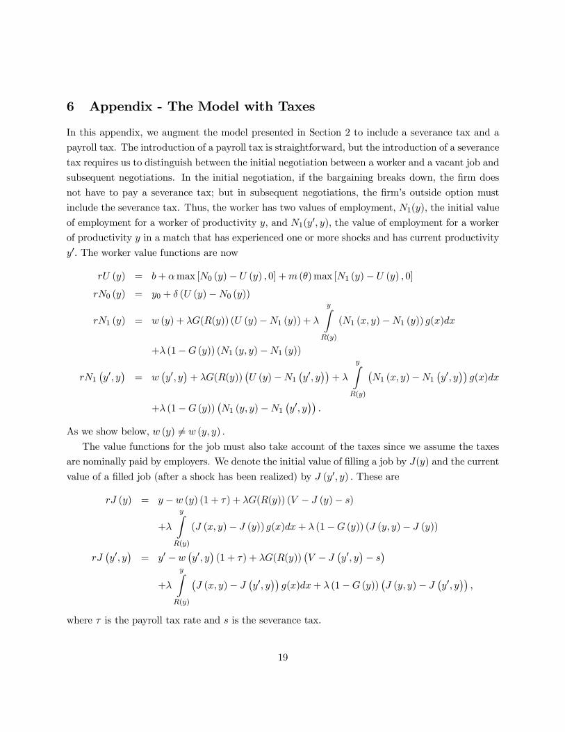
6 Appendix - The Model with Taxes

In this appendix, we augment the model presented in Section 2 to include a severance tax and a

payroll tax. The introduction of a payroll tax is straightforward, but the introduction of a severance

tax requires us to distinguish between the initial negotiation between a worker and a vacant job and

subsequent negotiations. In the initial negotiation, if the bargaining breaks down, the firm does

not have to pay a severance tax; but in subsequent negotiations, the firm’s outside option must

include the severance tax. Thus, the worker has two values of employment, N1(y), the initial value

of employment for a worker of productivity y, and N1(y0, y), the value of employment for a workerof productivity y in a match that has experienced one or more shocks and has current productivity

y0. The worker value functions are now

rU (y) = b+ αmax [N0 (y)− U (y) , 0] +m (θ)max [N1 (y)− U (y) , 0]

rN0 (y) = y0 + δ (U (y)−N0 (y))

rN1 (y) = w (y) + λG(R(y)) (U (y)−N1 (y)) + λ

yZR(y)

(N1 (x, y)−N1 (y)) g(x)dx

+λ (1−G (y)) (N1 (y, y)−N1 (y))

rN1¡y0, y

¢= w

¡y0, y

¢+ λG(R(y))

¡U (y)−N1

¡y0, y

¢¢+ λ

yZR(y)

¡N1 (x, y)−N1

¡y0, y

¢¢g(x)dx

+λ (1−G (y))¡N1 (y, y)−N1

¡y0, y

¢¢.

As we show below, w (y) 6= w (y, y) .

The value functions for the job must also take account of the taxes since we assume the taxes

are nominally paid by employers. We denote the initial value of filling a job by J(y) and the current

value of a filled job (after a shock has been realized) by J (y0, y) . These are

rJ (y) = y −w (y) (1 + τ) + λG(R(y)) (V − J (y)− s)

+λ

yZR(y)

(J (x, y)− J (y)) g(x)dx+ λ (1−G (y)) (J (y, y)− J (y))

rJ¡y0, y

¢= y0 −w

¡y0, y

¢(1 + τ) + λG(R(y))

¡V − J

¡y0, y

¢− s¢

+λ

yZR(y)

¡J (x, y)− J

¡y0, y

¢¢g(x)dx+ λ (1−G (y))

¡J (y, y)− J

¡y0, y

¢¢,

where τ is the payroll tax rate and s is the severance tax.

19

The value of a vacancy is now

rV = −c+ m(θ)

θEmax[J(y)− V, 0].

The initial wage w(y) for a worker of type y solves

maxw(y)

[N1(y)− U(y)]βJ(y)1−β,

while the wage w (y0, y) for a type y worker producing at y0 solves

maxw(y0,y)

[N1(y0, y)− U(y)]β

£J(y0, y) + s

¤1−β.

The initial wage and the subsequent wages can then be written as

w (y) =β (y − λs) + (1− β)(1 + τ)rU(y)

1 + τ

w¡y0, y

¢=

β (y0 + rs) + (1− β)(1 + τ)rU(y)

1 + τ.

Note that this introduces a complication into the distributional analysis; namely, conditional on y,

the density of wages now has two mass points, one at w(y) and one at w(y, y).

When there is a severance tax, the reservation productivity is defined by

N1(R (y) , y)− U(y) + J (R (y) , y) = −s.

Given the surplus sharing rule, this is equivalent to J (R (y) , y) = −s. Substitution gives

R(y) = (1 + τ)rU (y)− sr − λ

r + λ

Z y

R(y)[1−G(x)]dx. (A1)

This makes it clear that s shifts the R(y) schedule down, while τ shifts it up.

We can now solve for y∗ and y∗∗. The first cutoff value when taxes are included is given by

y∗ = (1 + τ)b (r + δ) + αy0

r + α+ δ+ λs− λ

r + λ

Z y∗

R(y∗)(1−G (x)) dx.

As in the basic model, since R(y) is increasing in θ, y∗ is also increasing in θ. The second cutoff

value, y∗∗, is given by

y∗∗ = (1 + τ)(y0 − b)(r + λ) +m (θ)βy0

m (θ)β+ λs− λ

r + λ

Z y∗∗

R(y∗∗)[1−G(x)]dx.

The flow value of unemployment, rU(y), for y ≤ y∗ does not depend on y or on taxes and is

given by

rU (y) =b (r + δ) + αy0

r + α+ δ.

20

For y∗ ≤ y < y∗∗, we have

rU (y) =[b (r + δ) + αy0] (r + λ) + (r+δ)m(θ)β

1+τ

ny − λs+ λ

r+λ

R yR(y)[1−G(x)]dx

o(r + α+ δ) (r + λ) + (r + δ)m (θ)β

and for y ≥ y∗∗, we have

rU (y) =b (r + λ) + m(θ)β

1+τ

ny − λs+ λ

r+λ

R yR(y)[1−G(x)]dx

or + λ+m (θ)β

.

As in the model with no taxes, there are unique solutions for y∗ and y∗∗ given θ.

The model’s steady-state conditions are the same as those given in the text and so are not

repeated here. Finally, we use the free-entry condition to close the model and determine equilibrium

labor market tightness. Setting V = 0 we have

c =m(θ)

θEmax[J(y), 0].

After substitution, the free-entry condition is

c =m (θ) (1− β)

θ

Z 1

y∗

µy −R (y)

r + λ− s

1− β

¶u (y)

uf(y)dy. (A2)

A unique equilibrium exists if there is a unique value of θ that solves equation (A2), taking into

account that R(y), u(y), and y∗ all depend on θ. As in the basic model,

1. R(y) is increasing in θ for each y;

2.R 1y∗

u(y)u f(y)dy is decreasing in θ;

3. y∗ is increasing in θ.

Given J(y) > 0 for y ≥ y∗, these three facts imply that the right-hand side of the free-entrycondition is decreasing in θ. This result, together with the facts that the limit of the right-hand side

of (A2) as θ → 0 equals ∞ and equals 0 as θ → ∞, implies the existence of a unique θ satisfying

the free-entry condition.

In order to ensure that J(y) > 0, we need to impose conditions that restrict the values of s and

τ . From equation (A2) a sufficient condition is

s <1

r + λ,

and from the reservation productivity schedule (equation A1),

R(y) +λ

r + λ

Z y

R(y)[1−G(x)]dx = (1 + τ)rU (y)− sr.

21

The term on the right-hand side must be positive. Then, given that rU (y) is increasing in y, it is

sufficient to check that (1 + τ)rU (y∗)− sr > 0, which in turn requires that

1 > (1 + τ)b (r + δ) + αy0

r + α+ δ> sr.

22

References

[1] Benhabib J., R. Rogerson and R. Wright (1991) “Homework in Macroeconomics: Household

Production and Aggregate Fluctuations,” Journal of Political Economy, 99, 1166-1187.

[2] Boeri T. and P. Garibaldi (2005), “Shadow Sorting,” NBER International Seminar on Macro-

economics 2005, MIT Press, forthcoming.

[3] Dolado, J., M. Jansen, and J. Jimeno (2005), “Dual Employment Protection Legislation: A

Framework for Analysis,” IZA Discussion Paper # 1564.

[4] Fugazza M. and J. Jacques (2003), “Labor Market Institutions, Taxation and the Underground

Economy,” Journal of Public Economics, 88, 395-418.

[5] Gong, X. and A. van Soest (2002), “Wage Differentials and Mobility in the Urban Labour

Market: A Panel Data Analysis for Mexico,” Labour Economics, 9, 513-529.

[6] Heckman, J. and C. Pagés (2004), Law and Employment: Lessons from Latin America and the

Caribean, editors, NBER and University of Chicago Press.

[7] Kolm A. and B. Larsen (2003), “Social Norm, the informal sector and unemployment,” Fi-

nanzArchiv, 59, 407-424.

[8] Kugler, A. (1999), “The Impact of Firing Costs on Turnover and Unemployment: Evidence

from the Colombian Labor Market Reforms,” International Tax and Public Finance, 6, 389-

410.

[9] Kugler, A. and M. Kugler (2003), “The Labor Market Effects of a Payroll Tax in a Middle-

Income Country: Evidence from Colombia,” mimeo.

[10] Masatlioglu W. and J. Rigolini (2005), “Labor Dynamics and the Informal Economy,” mimeo.

[11] Maloney, W (1999), “Does Informality Imply Segmentation in Urban Labor Markets? Evidence

from Sectoral Transitions in Mexico,” World Bank Economic Review, 13, 275-302.

[12] Maloney, W. (2004), “Informality Revisited,” World Development, 32, 1159-1178.

[13] Mortensen, D. and C. Pissarides (1994), “Job Creation and Job Destruction in the Theory of

Unemployment,” Review of Economic Studies, 61, 397-415.

[14] Mortensen, D. and C. Pissarides (1999), “Job Reallocation, Employment Fluctuations and

Unemployment," Handbook of Macroeconomics, Volume I, Edited by J. B. Taylor and M.

Woodford, Elsevier Science.

23

[15] Mortensen D. and C. Pissarides (2003), “Taxes, Subsidies and Equilibrium Labor Market

Outcomes,” in Designing Inclusion: Tools to Raise Low-End Pay and Employment in Private

Enterprise, edited by Edmund S. Phelps, Cambridge: Cambridge University Press.

[16] Parente S., R. Rogerson and R. Wright (2000) “Homework in Development Economics: House-

hold Production and the Wealth of Nations,” Journal of Political Economy, 108, 680-687.

[17] Schneider, F. and D. Enste (2000), “Shadow Economies: Sizes, Causes, Consequences,” Journal

of Economic Literature, 38, 77-114

24

Table 1: Effects of Varying s with τ = 0

u rates by type formal output

s θ y∗ y∗∗ R(y∗) R(y∗∗) low med high total y0 w Y

0 1.21 0.315 0.410 0.315 0.243 0.091 0.037 0.091 0.086 0.639 0.579 0.459

.05 1.12 0.331 0.425 0.278 0.200 0.091 0.035 0.085 0.082 0.631 0.562 0.458

.1 1.03 0.345 0.439 0.240 0.153 0.091 0.031 0.079 0.078 0.617 0.544 0.453

.15 0.94 0.357 0.451 0.200 0.104 0.091 0.027 0.071 0.074 0.601 0.528 0.448

.2 0.85 0.368 0.458 0.158 0.049 0.091 0.021 0.061 0.068 0.578 0.510 0.440

Table 2: Effects of Varying τ with s = 0

u rates by type formal output

τ θ y∗ y∗∗ R(y∗) R(y∗∗) low med high total y0 w Y

0 1.21 0.315 0.410 0.315 0.243 0.091 0.037 0.091 0.086 0.639 0.579 0.459

0.05 1.19 0.331 0.434 0.331 0.257 0.091 0.039 0.093 0.087 0.647 0.560 0.459

0.1 1.17 0.347 0.459 0.347 0.272 0.091 0.040 0.095 0.088 0.656 0.540 0.458

0.15 1.15 0.363 0.484 0.363 0.287 0.091 0.041 0.098 0.088 0.665 0.524 0.456

0.2 1.12 0.378 0.511 0.378 0.302 0.091 0.043 0.100 0.089 0.675 0.509 0.455

Table 3: Results with s = τ = 0 and s = τ = 0.1

u rates by type formal output

θ y∗ y∗∗ R(y∗) R(y∗∗) low med high total y0 w Y

1.21 0.315 0.410 0.315 0.243 0.091 0.037 0.091 0.086 0.639 0.579 0.459

0.98 0.380 0.495 0.275 0.186 0.091 0.035 0.084 0.081 0.636 0.509 0.451

25

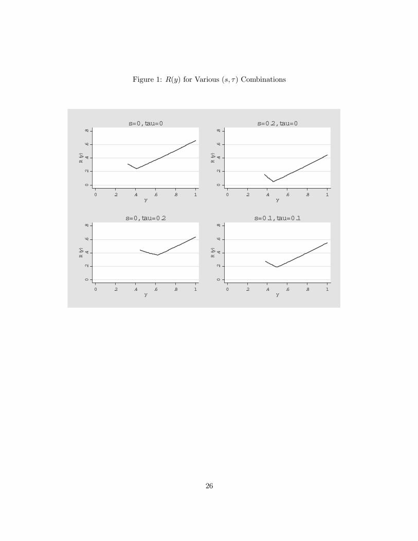
Figure 1: R(y) for Various (s, τ) Combinations0

.2.4

.6.8

R(y)

0 .2 .4 .6 .8 1y

s=0, tau=0

0.2

.4.6

.8R(y)

0 .2 .4 .6 .8 1y

s=0.2, tau=0

0.2

.4.6

.8R(y)

0 .2 .4 .6 .8 1y

s=0, tau=0.20

.2.4

.6.8

R(y)

0 .2 .4 .6 .8 1y

s=0.1, tau=0.1

26

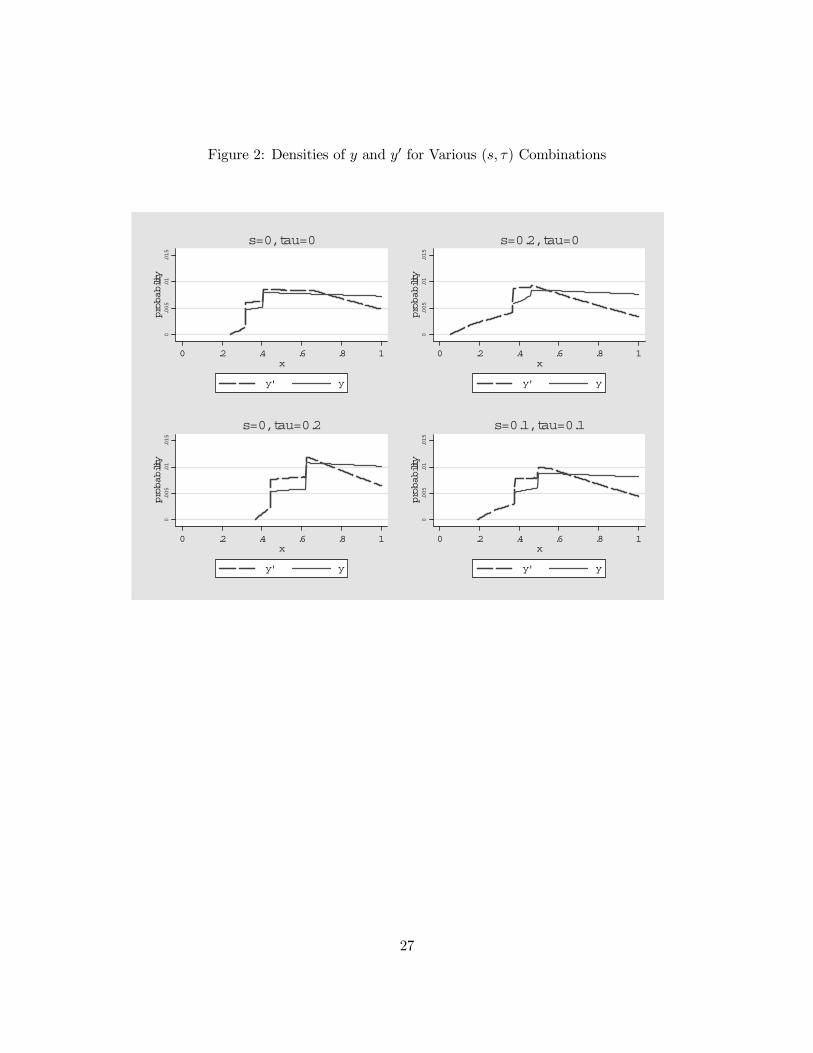
Figure 2: Densities of y and y0 for Various (s, τ) Combinations0

.005

.01

.015

probability

0 .2 .4 .6 .8 1x

y' y

s=0, tau=0

0.005

.01

.015

probability

0 .2 .4 .6 .8 1x

y' y

s=0.2, tau=0

0.005

.01

.015

probability

0 .2 .4 .6 .8 1x

y' y

s=0, tau=0.20

.005

.01

.015

probability

0 .2 .4 .6 .8 1x

y' y

s=0.1, tau=0.1

27

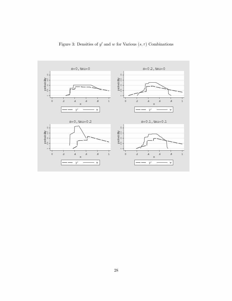
Figure 3: Densities of y0 and w for Various (s, τ) Combinations0

.005

.01

.015

.02

probability

0 .2 .4 .6 .8 1x

y' w

s=0, tau=0

0.005

.01

.015

.02

probability

0 .2 .4 .6 .8 1x

y' w

s=0.2, tau=0

0.005

.01

.015

.02

probability

0 .2 .4 .6 .8 1x

y' w

s=0, tau=0.20

.005

.01

.015

.02

probability

0 .2 .4 .6 .8 1x

y' w

s=0.1, tau=0.1

28