Embed Size (px)
Citation preview
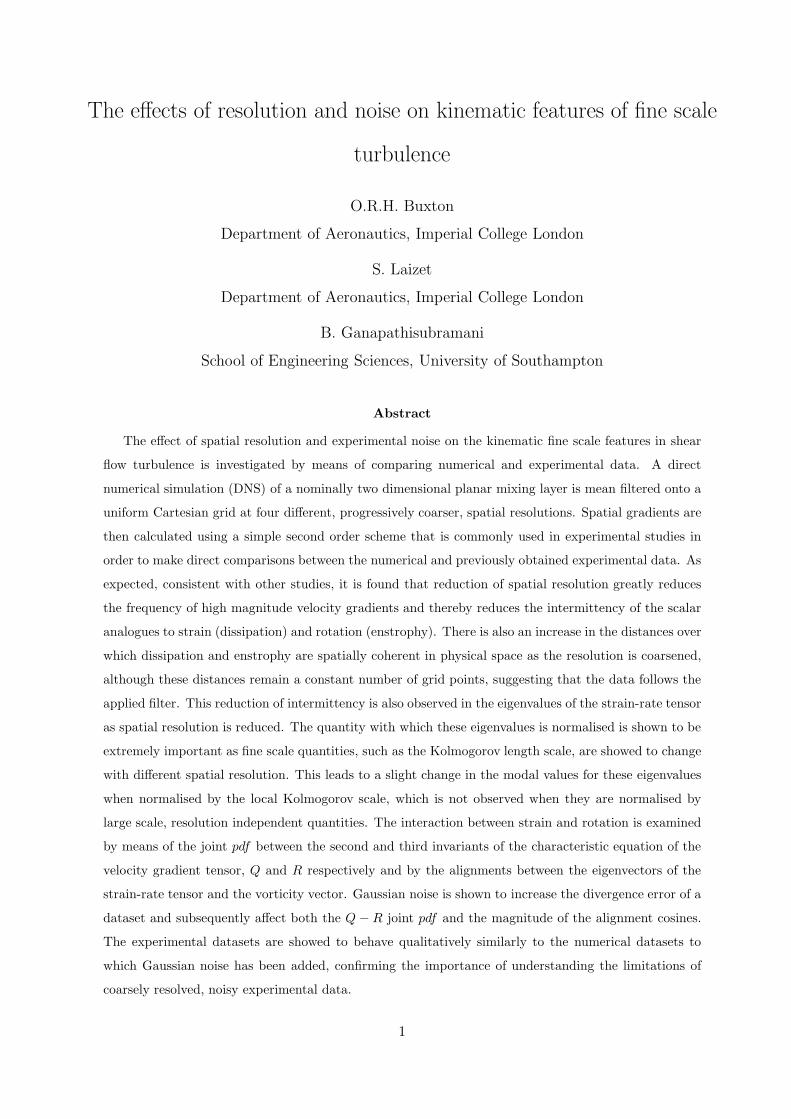
The effects of resolution and noise on kinematic features of fine scale
turbulence
O.R.H. Buxton
Department of Aeronautics, Imperial College London
S. Laizet
Department of Aeronautics, Imperial College London
B. Ganapathisubramani
School of Engineering Sciences, University of Southampton
Abstract
The effect of spatial resolution and experimental noise on the kinematic fine scale features in shear
flow turbulence is investigated by means of comparing numerical and experimental data. A direct
numerical simulation (DNS) of a nominally two dimensional planar mixing layer is mean filtered onto a
uniform Cartesian grid at four different, progressively coarser, spatial resolutions. Spatial gradients are
then calculated using a simple second order scheme that is commonly used in experimental studies in
order to make direct comparisons between the numerical and previously obtained experimental data. As
expected, consistent with other studies, it is found that reduction of spatial resolution greatly reduces
the frequency of high magnitude velocity gradients and thereby reduces the intermittency of the scalar
analogues to strain (dissipation) and rotation (enstrophy). There is also an increase in the distances over
which dissipation and enstrophy are spatially coherent in physical space as the resolution is coarsened,
although these distances remain a constant number of grid points, suggesting that the data follows the
applied filter. This reduction of intermittency is also observed in the eigenvalues of the strain-rate tensor
as spatial resolution is reduced. The quantity with which these eigenvalues is normalised is shown to be
extremely important as fine scale quantities, such as the Kolmogorov length scale, are showed to change
with different spatial resolution. This leads to a slight change in the modal values for these eigenvalues
when normalised by the local Kolmogorov scale, which is not observed when they are normalised by
large scale, resolution independent quantities. The interaction between strain and rotation is examined
by means of the joint pdf between the second and third invariants of the characteristic equation of the
velocity gradient tensor, Q and R respectively and by the alignments between the eigenvectors of the
strain-rate tensor and the vorticity vector. Gaussian noise is shown to increase the divergence error of a
dataset and subsequently affect both the Q − R joint pdf and the magnitude of the alignment cosines.
The experimental datasets are showed to behave qualitatively similarly to the numerical datasets to
which Gaussian noise has been added, confirming the importance of understanding the limitations of
coarsely resolved, noisy experimental data.
1
1 Introduction
The last twenty years or so has seen the development of experimental techniques that provide access to
all nine components of the velocity gradient tensor, Dij = ∂ui/∂xj . Wallace and Vukoslavcevic [2010]
provide a review of studies capable of measuring the full velocity gradient tensor from the use of hot wires
to optical techniques such as particle tracking velocimetry (PTV) and particle image velocimetry (PIV).
The dynamics of Dij have provoked great interest since the work of Vieillefosse [1982]. This has primarily
been driven by the interest in the interaction between the strain-rate (Sij) and rotation (Ωij) tensors,
the symmetric and skew-symmetric components of Dij respectively. This interaction has been described
as “intrinsic to the very nature of three dimensional turbulence” [Tennekes and Lumley, 1972; Bermejo-
Moreno et al., 2009]. The strain - rotation interaction is a fine scale feature of turbulent flows, taking place
over length scales comparable to the Kolmogorov (dissipative) length scale. Measuring these quantities
experimentally is exceedingly challenging as very few three dimensional experimental studies are capable
of resolving these scales, and the examination of under resolved data can skew our understanding of this
interaction.
Full three dimensional velocity fields and the complete velocity gradient tensor can now be obtained
through various diagnostic methods. The complete velocity gradient tensor can be obtained at a single
point using the multi-point hot-wire technique [Vukoslavcevic et al., 1991; Tsinober et al., 1992]. The
cinematographic stereoscopic PIV studies of Ganapathisubramani et al. [2007, 2008] performed stereo PIV
measurements in a plane normal to the streamwise direction and used Taylor hypothesis to calculate the
streamwise components of the velocity gradient tensor (with the other gradients computed in the plane of
measurement). Tao et al. [2000, 2002]; van der Bos et al. [2002], using holographic PIV, Mullin and Dahm
[2006]; Ganapathisubramani et al. [2005] using dual-plane stereoscopic PIV, and, Worth [2010]; Worth
et al. [2010], using tomographic PIV, were able to directly compute all nine components of the velocity
gradient tensor without resorting to use of the Taylor hypothesis. Additionally, a three dimensional particle
tracking velocimetry (3D-PTV) technique has been developed by Luthi et al. [2005]; Kinzel et al. [2010]
to experimentally measure all the components of the velocity gradient tensor in a Lagrangian way. All of
these above-mentioned studies explored the kinematic features of fine-scale turbulence including alignment
between the eigenvectors of the strain-rate tensor and the vorticity vector, and the joint probability density
functions (pdfs) of the invariants of velocity gradient tensor. Whilst these studies reported qualitatively
similar findings there are some quantitative differences in, for example, the peak values of the strain -
rotation alignment pdfs. This is perhaps attributable to different spatial resolution achieved in these
techniques and/or the experimental noise present in the data. It is thus extremely important to determine
2
the effect that spatial resolution and experimental noise play in observing the physics of the strain -
rotation interaction. This interaction is inherently multi-scale in nature, and some aspects of it will not
be observable at coarser resolutions, thereby distorting our understanding of the physical processes that
underpin it.
Previous work on the resolution effects of measurement of fine-sale turbulence has shown that coarsely
resolved data underestimates quantities such as enstrophy (ω2i ) and dissipation (ǫ = 2νSijSij), the scalar
counterparts to rotation and strain-rate respectively [Lavoie et al., 2007]. More coarsely resolved data also
does not tend to “pick up” the extreme events, several thousand times the mean [Donzis et al., 2008], that
is so important in fine-scale turbulence [Tsinober, 1998]. Coarsely resolved data has also been shown to
increase the physical length scales over which ω2i and ǫ are spatially coherent [Worth, 2010]. In addition
to the problem of limited resolution experimental studies suffer from the presence of experimental noise,
in particular on the velocity gradients. Christensen and Adrian [2002] describe the three main sources of
noise on PIV velocity fields as being random error due to electrical noise within the camera, bias error due
to pixel peak locking etc. and gradient noise due to local random velocity gradients within the flow. These
errors are further discussed in Westerweel [2000]. Although methods can be found to ameliorate some
of these errors, such as pixel peak locking [Christensen, 2004], they can never be completely eliminated.
The effect of experimental noise is investigated by Lund and Rogers [1994]. They show that qualitatively
similar results can be found when comparing probability density functions (pdfs) formed from the hot wire
data of Tsinober et al. [1992] and their DNS results to which Gaussian noise has been added. They state
that the divergence error introduced into the data as a result of this noise is of great significance to pdfs
of quantities such as the eigenvalues of the rate of strain tensor.
Given that advanced techniques aim to capture kinematics and dynamics of fine-scale turbulence, it
is essential that we understand the effects of resolution and noise on our observations and conclusions.
This study, therefore, sets out to examine the effects of spatial resolution and experimental noise on the
observation of the velocity gradient tensor, and its kinematic features in fine scale turbulence. First,
the effect of resolution is examined using data from the self-similar region of a direct numerical simulation
(DNS) of a nominally two dimensional planar mixing layer that is filtered at four different spatial resolutions
and compared to the “best case” original dataset. Second, the effect of noise on the kinematics of fine-scale
turbulence is explored by adding zero mean Gaussian noise to the four mean filtered datasets. This data is
then compared against experimental data, which comes from Ganapathisubramani et al. [2007], taken in
the far field of a turbulent axisymmetric jet. It will thus present the effects of coarsening spatial resolution
and experimental noise on the velocity gradients and explore how this influences the observation of strain
and rotation, which is crucial in furthering the experimental observation of the strain - rotation interaction.
3
2 Experimental and numerical methods
This study relies upon experimental data from the far field of an axisymmetric turbulent jet and data from
a direct numerical simulation of a nominally two dimensional planar mixing layer.
2.1 Experimental methods
The data used in this study was obtained by Ganapathisubramani et al. [2007]. The study examined the
turbulence in the far field of an axisymmetric turbulent jet which exhausted into a mild co-flow of air from
a pipe of circular cross-section of diameter 26 mm.
Cinematographic stereoscopic PIV measurements were performed in the “end view” plane (x2−x3) at a
downstream axial location of x1 = 32 pipe diameters. Further details regarding the experimental techniques
are available in Ganapathisubramani et al. [2007]. The relevant length scales at the measurement location
were : jet half-width (δ1/2) = 126 mm, Taylor microscale (λ) = 13.8 mm, Kolmogorov length scale (η)
= 0.45 mm. The Kolmogorov length scale is defined as η =(
ν3/〈ǫ〉)1/4
, where 〈ǫ〉 is the mean rate of
dissipation which is calculated directly from the experimental data and the Reynolds number based on
Taylor microscale is Reλ ≈ 150. Evidently there is no better estimate for the Kolmogorov length scale
than that calculated directly from the mean dissipation rate of the dataset and hence, unless otherwise
stated, this will be regarded as η for the experimental data as opposed to ηl, i.e. the “local” Kolmogorov
length scale.
The resolution of the stereoscopic vector fields is approximately 3η × 3η (1.35 mm × 1.35 mm) and
successive vectors are separated by 1.5η due to the 50% oversampling. The total field size is 160η × 160η
(76 mm × 76 mm). Taylor’s hypothesis with a convection velocity equal to the local mean axial velocity,
〈u1〉(x2, x3), was utilised to reconstruct a quasi-instantaneous space-time volume. This data was then
filtered with a Gaussian filter of filter width 3η in all three directions in order to reduce the spatial velocity
gradients’ noise levels. These spatial gradients were calculated with a second order central difference
scheme. Due to intrinsic uncertainties associated with performing stereoscopic PIV measurements the
velocity field was not divergence free (i.e. ∇·u 6= 0). The divergence error is in line with other experimental
studies and is characterised and discussed further in Ganapathisubramani et al. [2007].
2.2 Numerical methods
Direct numerical simulations of a nominally two dimensional planar mixing layer, generated by means of
two flows of different freestream velocities (U1 and U2) either side of a splitter plate of thickness h were
performed. The computational domain (Lx×Ly×Lz) = (230.4h×48h×28.8h) is discretised on a Cartesian
4
mesh (stretched in the cross-stream direction) of (nx × ny × nz) = (2049 × 513 × 256) mesh nodes. The
stretching of the mesh in the cross-stream direction leads to a minimal mesh size of ∆ymin ≈ 0.03h. The
time step, ∆t = 0.05h/Uc, where Uc = (U1 + U2)/2 is the mean convection velocity, is low enough to have
a CFL condition of about 0.3. The Reynolds number, ReW , based on Uc and h is 1000 and the Reynolds
number based on Taylor microscale, computed assuming isotropic turbulence [Taylor, 1935], is Reλ ≈ 180.
The boundary layers of thicknesses (corresponding to δ99) δ1 = 4h and δ2 = 3h are laminar with a
Blasius profile imposed at the inlet. They are submitted to residual 3D perturbations allowing a realistic
destabilisation of the flow downstream of the trailing edge. The spectral content of this artificial perturba-
tion is imposed to avoid the excitation of high wave numbers or frequency waves that cannot be correctly
described by the computational mesh. More details about the generation of the inlet/initial conditions can
be found in Laizet et al. [2010].
An in-house code (called “Incompact3d”) based on sixth order compact schemes for spatial discretisa-
tion and second order Adams-Bashforth scheme for time advancement is used to solve the incompressible
Navier-Stokes equations. To treat the incompressibility condition, a projection method is used, requiring
the solution of a Poisson equation for the pressure. This equation is fully solved in spectral space via the
use of the relevant three dimensional fast Fourier transforms (FFT) that allows the consideration of all the
combinations of free-slip, periodic or Dirichlet boundary conditions on the velocity field in the three spatial
directions. In the present calculations the boundary conditions are only inflow/outflow in the streamwise
direction (velocity boundary conditions of the Dirichlet type), free slip in the cross-stream direction at
y = −Ly/2 and Ly/2 and periodic in the spanwise direction at z = −Lz/2 and Lz/2. The pressure mesh
is staggered from the velocity mesh to avoid spurious pressure oscillations. Using the concept of modified
wavenumber, the divergence free condition is ensured up to the machine accuracy. More details about the
present code and its validation, especially the original treatment of the pressure in spectral space, can be
found in Laizet and Lamballais [2009].
2.3 Varying the resolution and computing spatial velocity gradients
A section of the computational domain, 301 mesh nodes in streamwise extent just upstream of the stream-
wise extent of the domain, was isolated. Three snapshots of this domain were saved a sufficient number
of time steps apart to ensure that all three realisations were statistically independent. This region of the
flow was shown to be in the self-similar region, meaning that fair comparisons between the computational
and experimental data could be made. A reference case was generated by calculating the spatial velocity
derivatives of this reduced domain using a modified version of the sixth order scheme. This reference case
is thus the “best case” of highest spatial resolution and highest order accurate numerical scheme on the
5
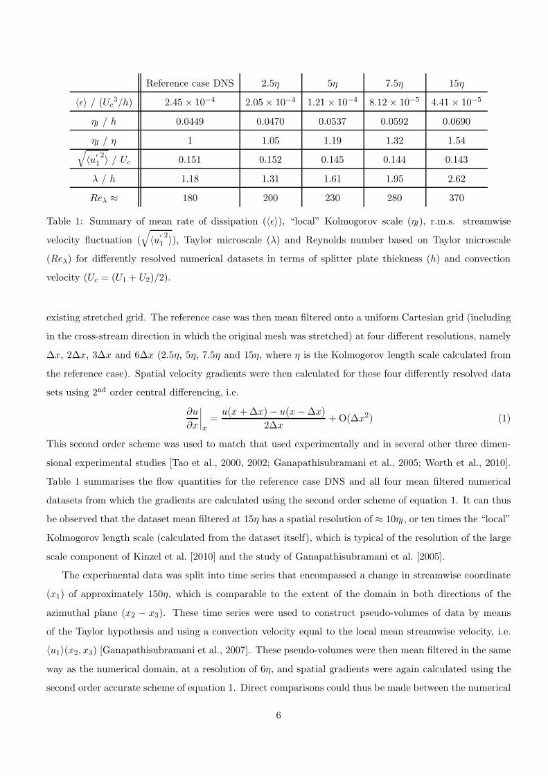
Reference case DNS 2.5η 5η 7.5η 15η
〈ǫ〉 / (Uc3/h) 2.45 × 10⁻⁴ 2.05 × 10⁻⁴ 1.21 × 10⁻⁴ 8.12 × 10⁻⁵ 4.41 × 10⁻⁵
ηl / h 0.0449 0.0470 0.0537 0.0592 0.0690
ηl / η 1 1.05 1.19 1.32 1.54√
〈u′
1
2〉 / Uc 0.151 0.152 0.145 0.144 0.143
λ / h 1.18 1.31 1.61 1.95 2.62
Reλ ≈ 180 200 230 280 370
Table 1: Summary of mean rate of dissipation (〈ǫ〉), “local” Kolmogorov scale (ηl), r.m.s. streamwise
velocity fluctuation (√
〈u′
1
2〉), Taylor microscale (λ) and Reynolds number based on Taylor microscale
(Reλ) for differently resolved numerical datasets in terms of splitter plate thickness (h) and convection
velocity (Uc = (U1 + U2)/2).
existing stretched grid. The reference case was then mean filtered onto a uniform Cartesian grid (including
in the cross-stream direction in which the original mesh was stretched) at four different resolutions, namely
∆x, 2∆x, 3∆x and 6∆x (2.5η, 5η, 7.5η and 15η, where η is the Kolmogorov length scale calculated from
the reference case). Spatial velocity gradients were then calculated for these four differently resolved data
sets using 2nd order central differencing, i.e.
∂u
∂x
∣
∣
∣
∣
x=
u(x + ∆x) − u(x − ∆x)
2∆x+ O(∆x2) (1)
This second order scheme was used to match that used experimentally and in several other three dimen-
sional experimental studies [Tao et al., 2000, 2002; Ganapathisubramani et al., 2005; Worth et al., 2010].
Table 1 summarises the flow quantities for the reference case DNS and all four mean filtered numerical
datasets from which the gradients are calculated using the second order scheme of equation 1. It can thus
be observed that the dataset mean filtered at 15η has a spatial resolution of ≈ 10ηl, or ten times the “local”
Kolmogorov length scale (calculated from the dataset itself), which is typical of the resolution of the large
scale component of Kinzel et al. [2010] and the study of Ganapathisubramani et al. [2005].
The experimental data was split into time series that encompassed a change in streamwise coordinate
(x1) of approximately 150η, which is comparable to the extent of the domain in both directions of the
azimuthal plane (x2 − x3). These time series were used to construct pseudo-volumes of data by means
of the Taylor hypothesis and using a convection velocity equal to the local mean streamwise velocity, i.e.
〈u1〉(x2, x3) [Ganapathisubramani et al., 2007]. These pseudo-volumes were then mean filtered in the same
way as the numerical domain, at a resolution of 6η, and spatial gradients were again calculated using the
second order accurate scheme of equation 1. Direct comparisons could thus be made between the numerical
6
data, at the various resolutions, and the experimental data at both resolutions with all of the gradients
being second order accurate.
3 Results and discussion
3.1 Effects of spatial resolution
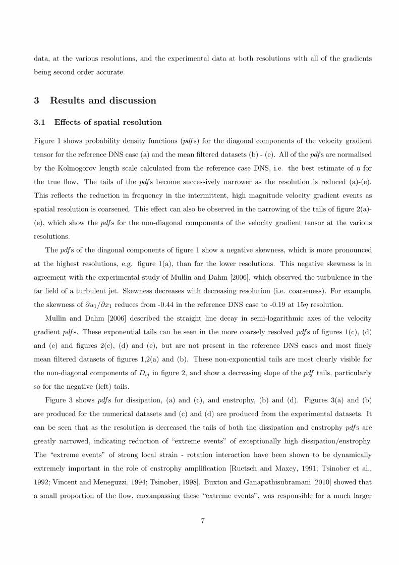
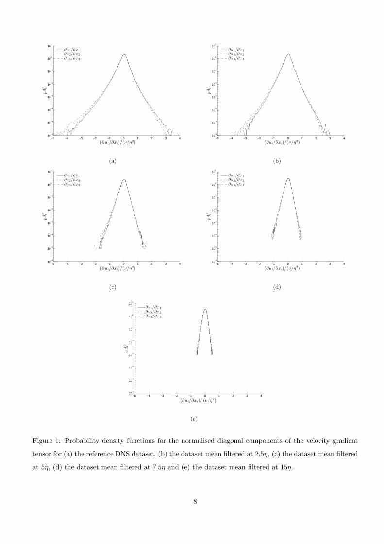
Figure 1 shows probability density functions (pdfs) for the diagonal components of the velocity gradient
tensor for the reference DNS case (a) and the mean filtered datasets (b) - (e). All of the pdfs are normalised
by the Kolmogorov length scale calculated from the reference case DNS, i.e. the best estimate of η for
the true flow. The tails of the pdfs become successively narrower as the resolution is reduced (a)-(e).
This reflects the reduction in frequency in the intermittent, high magnitude velocity gradient events as
spatial resolution is coarsened. This effect can also be observed in the narrowing of the tails of figure 2(a)-
(e), which show the pdfs for the non-diagonal components of the velocity gradient tensor at the various
resolutions.
The pdfs of the diagonal components of figure 1 show a negative skewness, which is more pronounced
at the highest resolutions, e.g. figure 1(a), than for the lower resolutions. This negative skewness is in
agreement with the experimental study of Mullin and Dahm [2006], which observed the turbulence in the
far field of a turbulent jet. Skewness decreases with decreasing resolution (i.e. coarseness). For example,
the skewness of ∂u1/∂x1 reduces from -0.44 in the reference DNS case to -0.19 at 15η resolution.
Mullin and Dahm [2006] described the straight line decay in semi-logarithmic axes of the velocity
gradient pdfs. These exponential tails can be seen in the more coarsely resolved pdfs of figures 1(c), (d)
and (e) and figures 2(c), (d) and (e), but are not present in the reference DNS cases and most finely
mean filtered datasets of figures 1,2(a) and (b). These non-exponential tails are most clearly visible for
the non-diagonal components of Dij in figure 2, and show a decreasing slope of the pdf tails, particularly
so for the negative (left) tails.
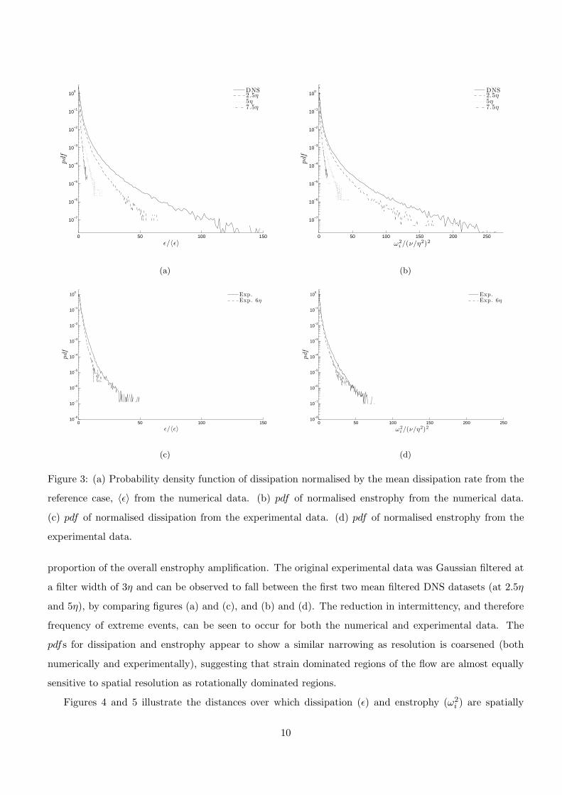
Figure 3 shows pdfs for dissipation, (a) and (c), and enstrophy, (b) and (d). Figures 3(a) and (b)
are produced for the numerical datasets and (c) and (d) are produced from the experimental datasets. It
can be seen that as the resolution is decreased the tails of both the dissipation and enstrophy pdfs are
greatly narrowed, indicating reduction of “extreme events” of exceptionally high dissipation/enstrophy.
The “extreme events” of strong local strain - rotation interaction have been shown to be dynamically
extremely important in the role of enstrophy amplification [Ruetsch and Maxey, 1991; Tsinober et al.,
1992; Vincent and Meneguzzi, 1994; Tsinober, 1998]. Buxton and Ganapathisubramani [2010] showed that
a small proportion of the flow, encompassing these “extreme events”, was responsible for a much larger
7
−5 −4 −3 −2 −1 0 1 2 3 410
−6
10−5
10−4
10−3
10−2
10−1
100
101
(∂ui/∂xi)/(ν/η2)
∂u1/∂x1
∂u2/∂x2
∂u3/∂x3
(a)
−5 −4 −3 −2 −1 0 1 2 3 410
−6
10−5
10−4
10−3
10−2
10−1
100
101
(∂ui/∂xi)/(ν/η2)
∂u1/∂x1
∂u2/∂x2
∂u3/∂x3
(b)
−5 −4 −3 −2 −1 0 1 2 3 410
−6
10−5
10−4
10−3
10−2
10−1
100
101
(∂ui/∂xi)/(ν/η2)
∂u1/∂x1
∂u2/∂x2
∂u3/∂x3
(c)
−5 −4 −3 −2 −1 0 1 2 3 410
−6
10−5
10−4
10−3
10−2
10−1
100
101
(∂ui/∂xi)/(ν/η2)
∂u1/∂x1
∂u2/∂x2
∂u3/∂x3
(d)
−5 −4 −3 −2 −1 0 1 2 3 410
−6
10−5
10−4
10−3
10−2
10−1
100
101
(∂ui/∂xi)/(
ν/η2)
∂u1/∂x1
∂u2/∂x2
∂u3/∂x3
(e)
Figure 1: Probability density functions for the normalised diagonal components of the velocity gradient
tensor for (a) the reference DNS dataset, (b) the dataset mean filtered at 2.5η, (c) the dataset mean filtered
at 5η, (d) the dataset mean filtered at 7.5η and (e) the dataset mean filtered at 15η.
8
−8 −6 −4 −2 0 2 4 6 8
10−6
10−5
10−4
10−3
10−2
10−1
100
101
(∂ui/∂xj)/(ν/η2)∣
∣
i 6=j
∂u1/∂x2
∂u1/∂x3
∂u2/∂x1
∂u2/∂x3
∂u3/∂x1
∂u3/∂x2
(a)
−8 −6 −4 −2 0 2 4 6 8
10−6
10−5
10−4
10−3
10−2
10−1
100
101
(∂ui/∂xj)/(ν/η2)∣
∣
i 6=j
∂u1/∂x2
∂u1/∂x3
∂u2/∂x1
∂u2/∂x3
∂u3/∂x1
∂u3/∂x2
(b)
−8 −6 −4 −2 0 2 4 6 8
10−6
10−5
10−4
10−3
10−2
10−1
100
101
(∂ui/∂xj)/(ν/η2)∣
∣
i 6=j
∂u1/∂x2
∂u1/∂x3
∂u2/∂x1
∂u2/∂x3
∂u3/∂x1
∂u3/∂x2
(c)
−8 −6 −4 −2 0 2 4 6 8
10−6
10−5
10−4
10−3
10−2
10−1
100
101
(∂ui/∂xj)/(ν/η2)∣
∣
i 6=j
∂u1/∂x2
∂u1/∂x3
∂u2/∂x1
∂u2/∂x3
∂u3/∂x1
∂u3/∂x2
(d)
−8 −6 −4 −2 0 2 4 6 8
10−6
10−5
10−4
10−3
10−2
10−1
100
101
(∂ui/∂xj)/(
ν/η2)∣
∣
i 6=j
∂u1/∂x2
∂u1/∂x3
∂u2/∂x1
∂u2/∂x3
∂u3/∂x1
∂u3/∂x2
(e)
Figure 2: Probability density functions for the normalised non-diagonal components of the velocity gradient
tensor for (a) the reference DNS dataset, (b) the dataset mean filtered at 2.5η, (c) the dataset mean filtered
at 5η, (d) the dataset mean filtered at 7.5η and (e) the dataset mean filtered at 15η.
9
0 50 100 150
10−7
10−6
10−5
10−4
10−3
10−2
10−1
100
ǫ/〈ǫ〉
DNS2.5η5η7.5η
(a)
0 50 100 150 200 250
10−7
10−6
10−5
10−4
10−3
10−2
10−1
100
ω2
i /(ν/η2)2
DNS2.5η5η7.5η
(b)
0 50 100 15010
−8
10−7
10−6
10−5
10−4
10−3
10−2
10−1
100
ǫ/〈ǫ〉
Exp.Exp. 6η
(c)
0 50 100 150 200 25010
−8
10−7
10−6
10−5
10−4
10−3
10−2
10−1
100
ω2
i /(ν/η2)2
Exp.Exp. 6η
(d)
Figure 3: (a) Probability density function of dissipation normalised by the mean dissipation rate from the
reference case, 〈ǫ〉 from the numerical data. (b) pdf of normalised enstrophy from the numerical data.
(c) pdf of normalised dissipation from the experimental data. (d) pdf of normalised enstrophy from the
experimental data.
proportion of the overall enstrophy amplification. The original experimental data was Gaussian filtered at
a filter width of 3η and can be observed to fall between the first two mean filtered DNS datasets (at 2.5η
and 5η), by comparing figures (a) and (c), and (b) and (d). The reduction in intermittency, and therefore
frequency of extreme events, can be seen to occur for both the numerical and experimental data. The
pdfs for dissipation and enstrophy appear to show a similar narrowing as resolution is coarsened (both
numerically and experimentally), suggesting that strain dominated regions of the flow are almost equally
sensitive to spatial resolution as rotationally dominated regions.
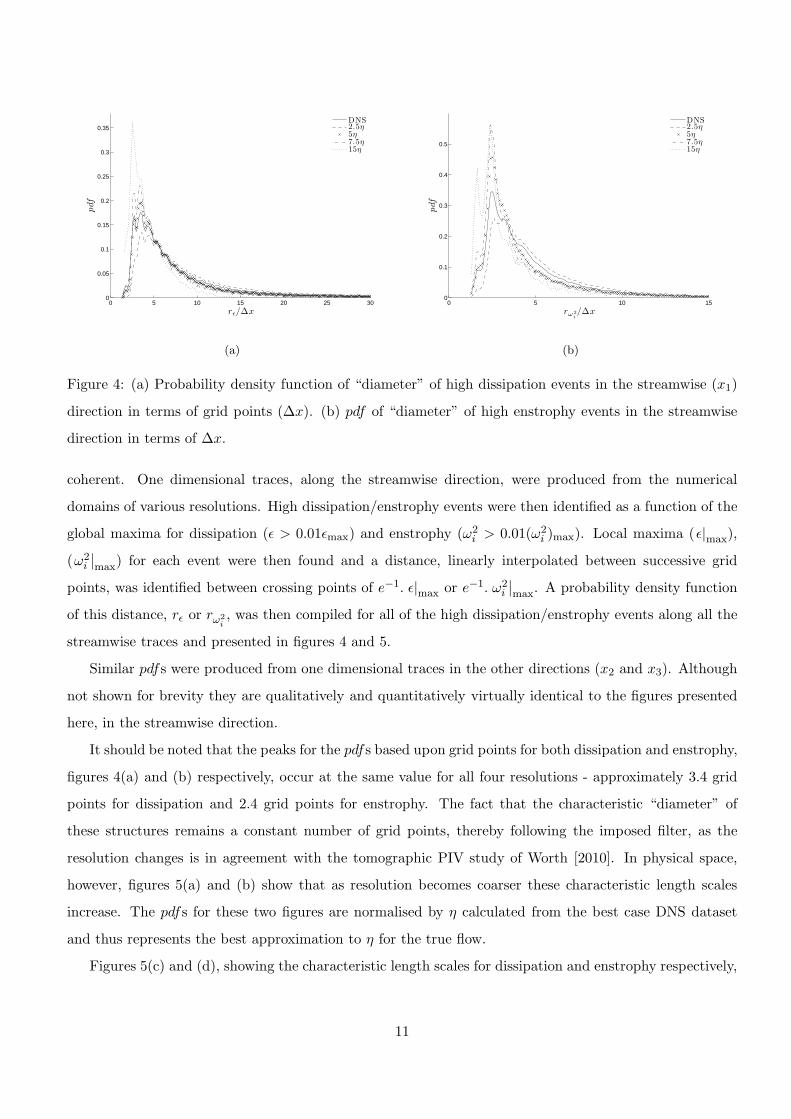
Figures 4 and 5 illustrate the distances over which dissipation (ǫ) and enstrophy (ω2i ) are spatially
10
0 5 10 15 20 25 300
0.05
0.1
0.15
0.2
0.25
0.3
0.35
rǫ/∆x
DNS2.5η5η7.5η15η
(a)
0 5 10 150
0.1
0.2
0.3
0.4
0.5
rω2
i
/∆x
DNS2.5η5η7.5η15η
(b)
Figure 4: (a) Probability density function of “diameter” of high dissipation events in the streamwise (x1)
direction in terms of grid points (∆x). (b) pdf of “diameter” of high enstrophy events in the streamwise
direction in terms of ∆x.
coherent. One dimensional traces, along the streamwise direction, were produced from the numerical
domains of various resolutions. High dissipation/enstrophy events were then identified as a function of the
global maxima for dissipation (ǫ > 0.01ǫmax) and enstrophy (ω2i > 0.01(ω2
i )max). Local maxima (ǫ|max
),
(ω2i
∣
∣
max) for each event were then found and a distance, linearly interpolated between successive grid
points, was identified between crossing points of e−1. ǫ|max
or e−1. ω2i
∣
∣
max. A probability density function
of this distance, rǫ or rω2
i
, was then compiled for all of the high dissipation/enstrophy events along all the
streamwise traces and presented in figures 4 and 5.
Similar pdfs were produced from one dimensional traces in the other directions (x2 and x3). Although
not shown for brevity they are qualitatively and quantitatively virtually identical to the figures presented
here, in the streamwise direction.
It should be noted that the peaks for the pdfs based upon grid points for both dissipation and enstrophy,
figures 4(a) and (b) respectively, occur at the same value for all four resolutions - approximately 3.4 grid
points for dissipation and 2.4 grid points for enstrophy. The fact that the characteristic “diameter” of
these structures remains a constant number of grid points, thereby following the imposed filter, as the
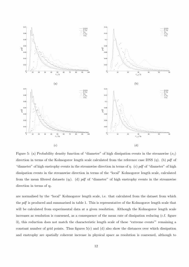
resolution changes is in agreement with the tomographic PIV study of Worth [2010]. In physical space,
however, figures 5(a) and (b) show that as resolution becomes coarser these characteristic length scales
increase. The pdfs for these two figures are normalised by η calculated from the best case DNS dataset
and thus represents the best approximation to η for the true flow.
Figures 5(c) and (d), showing the characteristic length scales for dissipation and enstrophy respectively,
11
0 10 20 30 40 50 60 70 80 90 1000
0.01
0.02
0.03
0.04
0.05
0.06
0.07
rǫ/η
DNS2.5η5η7.5η15η
(a)
0 10 20 30 40 50 600
0.02
0.04
0.06
0.08
0.1
0.12
0.14
rω2
i
/η
DNS2.5η5η7.5η15η
(b)
0 10 20 30 40 50 60 70 80 90 1000
0.01
0.02
0.03
0.04
0.05
0.06
0.07
rǫ/ηl
DNS2.5η5η7.5η15η
(c)
0 10 20 30 40 50 600
0.02
0.04
0.06
0.08
0.1
0.12
0.14
rω2
i
/ηl
DNS2.5η5η7.5η15η
(d)
Figure 5: (a) Probability density function of “diameter” of high dissipation events in the streamwise (x1)
direction in terms of the Kolmogorov length scale calculated from the reference case DNS (η). (b) pdf of
“diameter” of high enstrophy events in the streamwise direction in terms of η. (c) pdf of “diameter” of high
dissipation events in the streamwise direction in terms of the “local” Kolmogorov length scale, calculated
from the mean filtered datasets (ηl). (d) pdf of “diameter” of high enstrophy events in the streamwise
direction in terms of ηl.
are normalised by the “local” Kolmogorov length scale, i.e. that calculated from the dataset from which
the pdf is produced and summarised in table 1. This is representative of the Kolmogorov length scale that
will be calculated from experimental data at a given resolution. Although the Kolmogorov length scale
increases as resolution is coarsened, as a consequence of the mean rate of dissipation reducing (c.f. figure
3), this reduction does not match the characteristic length scale of these “extreme events’” remaining a
constant number of grid points. Thus figures 5(c) and (d) also show the distances over which dissipation
and enstrophy are spatially coherent increase in physical space as resolution is coarsened, although to
12
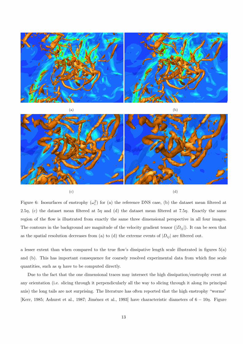
(a) (b)
(c) (d)
Figure 6: Isosurfaces of enstrophy (ω2i ) for (a) the reference DNS case, (b) the dataset mean filtered at
2.5η, (c) the dataset mean filtered at 5η and (d) the dataset mean filtered at 7.5η. Exactly the same
region of the flow is illustrated from exactly the same three dimensional perspective in all four images.
The contours in the background are magnitude of the velocity gradient tensor (|Dij |). It can be seen that
as the spatial resolution decreases from (a) to (d) the extreme events of |Dij | are filtered out.
a lesser extent than when compared to the true flow’s dissipative length scale illustrated in figures 5(a)
and (b). This has important consequence for coarsely resolved experimental data from which fine scale
quantities, such as ηl have to be computed directly.
Due to the fact that the one dimensional traces may intersect the high dissipation/enstrophy event at
any orientation (i.e. slicing through it perpendicularly all the way to slicing through it along its principal
axis) the long tails are not surprising. The literature has often reported that the high enstrophy “worms”
[Kerr, 1985; Ashurst et al., 1987; Jimenez et al., 1993] have characteristic diameters of 6 − 10η. Figure
13
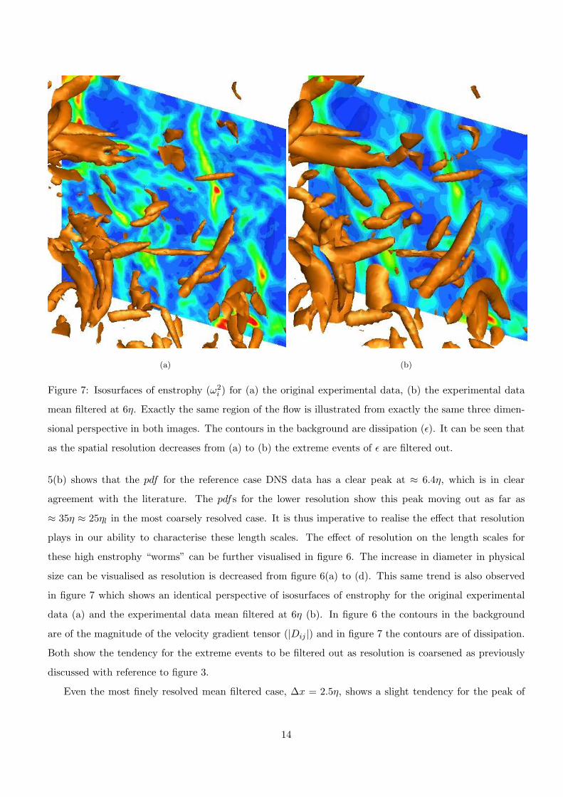
(a) (b)
Figure 7: Isosurfaces of enstrophy (ω2i ) for (a) the original experimental data, (b) the experimental data
mean filtered at 6η. Exactly the same region of the flow is illustrated from exactly the same three dimen-
sional perspective in both images. The contours in the background are dissipation (ǫ). It can be seen that
as the spatial resolution decreases from (a) to (b) the extreme events of ǫ are filtered out.
5(b) shows that the pdf for the reference case DNS data has a clear peak at ≈ 6.4η, which is in clear
agreement with the literature. The pdfs for the lower resolution show this peak moving out as far as
≈ 35η ≈ 25ηl in the most coarsely resolved case. It is thus imperative to realise the effect that resolution
plays in our ability to characterise these length scales. The effect of resolution on the length scales for
these high enstrophy “worms” can be further visualised in figure 6. The increase in diameter in physical
size can be visualised as resolution is decreased from figure 6(a) to (d). This same trend is also observed
in figure 7 which shows an identical perspective of isosurfaces of enstrophy for the original experimental
data (a) and the experimental data mean filtered at 6η (b). In figure 6 the contours in the background
are of the magnitude of the velocity gradient tensor (|Dij |) and in figure 7 the contours are of dissipation.
Both show the tendency for the extreme events to be filtered out as resolution is coarsened as previously
discussed with reference to figure 3.
Even the most finely resolved mean filtered case, ∆x = 2.5η, shows a slight tendency for the peak of
14
the pdf of figure 5(b) to move to a value greater than 6.4η. Ganapathisubramani et al. [2008] state that
these structures can be observed to be up to 40η in length based on a full-width of the structure at half the
maximum value criteria. Indeed, figure 5(b) shows that the pdf for the reference DNS case has not quite
reached zero at 60η, suggesting that a small proportion of these “worms” can stretch to a much greater
length than previously thought.
It should also be noted, by comparing figures 5(a) and (b), that the length scales over which high
dissipation events are spatially coherent are greater than those for enstrophy. This is due to the fact
that high dissipation events are often found to occur in regions in which the intermediate strain-rate
eigenvalue (s2) is positive [Ashurst et al., 1987]. This leads to “sheet-forming” topology, whereas high
enstrophy events are “tube-like” (“worms”). Sheets are spatially coherent over two dimensions, whereas
tubes are only spatially coherent (over any great distance) in one. In addition, the peaks of figure 5(a)
are at greater lengths than those of figure 5(b) (rǫ = 8.5η for the reference DNS case as opposed to
rω2
i
= 6.4η). This suggests that strain dominated regions of the flow are spatially coherent over greater
distances than rotationally dominated regions. It would therefore be expected that coarse resolution would
have a disproportionately more severe effect upon the observation of rotationally dominated regions of the
flow.
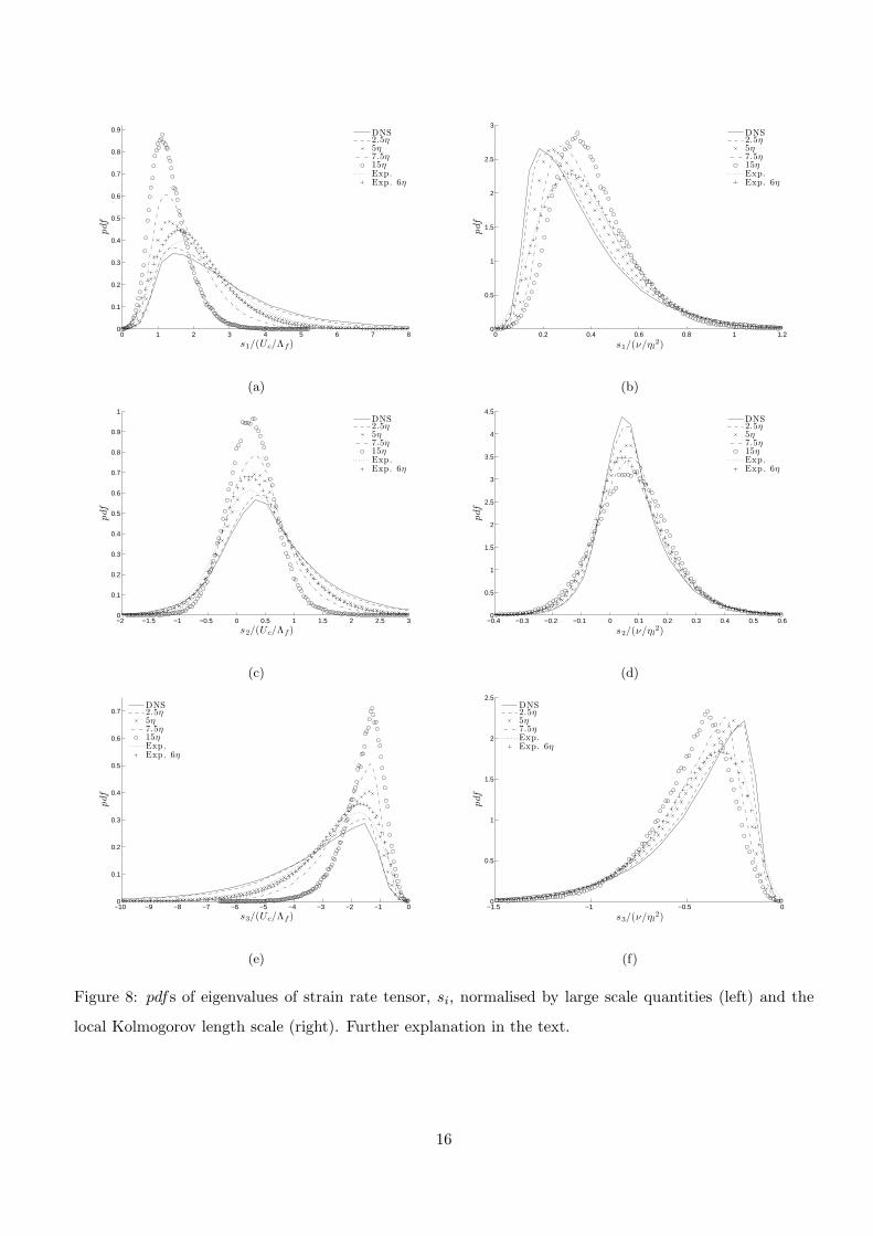
Figure 8 shows probability density functions for the eigenvalues of the strain-rate tensor for the reference
DNS dataset, the mean filtered datasets and the original and filtered experimental data. Figure 8(a) shows
the pdfs for the extensive strain-rate eigenvalue (s1), (c) shows the intermediate strain-rate eigenvalue (s2),
which can be either mildly extensive or compressive and is bounded by the values of s1 and s3 and (e)
shows the compressive strain-rate eigenvalue (s3) normalised by large scale quantities. Measuring small
scale quantities experimentally is both challenging and dependent upon the resolution of the experiment,
as illustrated by table 1 and the movement of the pdf peaks from figures 5(a) and (b) to their values in
figures 5(c) and (d) respectively.
Despite the fact that strain rates are fine scale features it is thus desirable to normalise them by large
scale quantities that are easier to measure and largely independent of the experiment’s resolution. The
quantity chosen is an inverse time scale formed as Uc/Λf , where Uc is a convection velocity and Λf is a
large scale vorticity thickness. For the numerical mixing layer Uc is defined as (U1 + U2)/2, or the mean
of the two free streams and for the experimental jet it is defined as the mean streamwise velocity along
the jet’s axis. The vorticity thickness for the mixing layer is defined as Λf = (U1 − U2)/∂〈u1〉∂x2
∣
∣
∣
maxat the
measurement location and as the jet half width at the measurement location for the jet flow. Figures 8(b),
(d) and (f) show s1, s2 and s3 normalised by the “local” Kolmogorov length scale respectively.
The reduction in intermittency as resolution is coarsened is again clearly visible in the figures. It can
15
0 1 2 3 4 5 6 7 80
0.1
0.2
0.3
0.4
0.5
0.6
0.7
0.8
0.9
s1/(Uc/Λf )
DNS2.5η5η7.5η15ηExp.Exp. 6η
(a)
0 0.2 0.4 0.6 0.8 1 1.20
0.5
1
1.5
2
2.5
3
s1/(ν/ηl2)
DNS2.5η5η7.5η15ηExp.Exp. 6η
(b)
−2 −1.5 −1 −0.5 0 0.5 1 1.5 2 2.5 30
0.1
0.2
0.3
0.4
0.5
0.6
0.7
0.8
0.9
1
s2/(Uc/Λf )
DNS2.5η5η7.5η15ηExp.Exp. 6η
(c)
−0.4 −0.3 −0.2 −0.1 0 0.1 0.2 0.3 0.4 0.5 0.60
0.5
1
1.5
2
2.5
3
3.5
4
4.5
s2/(ν/ηl2)
DNS2.5η5η7.5η15ηExp.Exp. 6η
(d)
−10 −9 −8 −7 −6 −5 −4 −3 −2 −1 00
0.1
0.2
0.3
0.4
0.5
0.6
0.7
s3/(Uc/Λf )
DNS2.5η5η7.5η15ηExp.Exp. 6η
(e)
−1.5 −1 −0.5 00
0.5
1
1.5
2
2.5
s3/(ν/ηl2)
DNS2.5η5η7.5ηExp.Exp. 6η
(f)
Figure 8: pdfs of eigenvalues of strain rate tensor, si, normalised by large scale quantities (left) and the
local Kolmogorov length scale (right). Further explanation in the text.
16
be seen that for all three strain-rate eigenvalues the tails of the pdfs are broader and, correspondingly, the
peak values at the modal value are lowest at the most highly resolved of the numerical and experimental
datasets and narrower and greater, respectively, at the coarsest resolution.
The large-scale normalised value at which the pdfs peak remains constant, though, as resolution is
coarsened for all three strain-rate eigenvalues. This suggests that the coarsening of resolution affects the
extreme strain-rate events, at the tails of the pdfs and not the modal events. It can thus be deduced that
the high magnitude strain-rates are spatially coherent over small distances and are thus “filtered out” at
coarser resolution. This is in agreement with Ganapathisubramani et al. [2008] which showed that the
large magnitude negative values of s2 are “spotty” and not spatially coherent over large distances and that
high magnitude positive values of s2 are “sheet-like”, with the thicknesses of these sheets being of the order
of ≈ 10η.
In contrast to the large scale normalised pdfs, those that are normalised by the “local” Kolmogorov
length scale show a variation in the location of the modal values. This effect is particularly pronounced
for s1 and s3. This again has serious implications for coarsely resolved experimental studies. The modal
location of the strains remain unchanged for different resolutions when normalised by large scale quantities
or the true Kolmogorov scale of the flow. However, this feature will not be observed when the strains are
normalised by dissipative quantities calculated from the data, due to the variation of the Kolmogorov scale
(ηl) with resolution.
The experimental and numerical data both show a similar position for the peak location of the interme-
diate strain-rate at s2 ≈ 0.04ν/ηl2. The intermediate strain-rate is responsible for determining the nature
of the topological evolution of a fluid element. When s2 is positive a fluid element is subjected to two
orthogonal extensive strain-rates and a further compressive strain-rate in the third, orthogonal, direction.
This leads to the formation of “sheet-like” topology. In contrast when a fluid element is subjected to two
orthogonal compressive strain-rates and a third orthogonal extensive strain-rate, i.e. s2 is negative, it will
evolve into a “tube” or “worm-like” structure. The sign and magnitude of the intermediate strain-rate
eigenvalue is thus of great physical significance to the topological evolution of a fluid element. Figures 8(c)
and (d) show that there is a clear preference in shear flow turbulence, both from the experimental jet flow
and the numerical mixing layer (at all spatial resolutions) for “sheet-forming” topological evolution over
“tube-forming” topological evolution.
3.2 Effects of experimental noise and spatial resolution
The effect of noise on the kinematics of fine-scale turbulence is explored by adding random noise to the
filtered DNS data. The noise is added such that the variance, σ, of the Gaussian function for all four
17
spatial resolutions is identical. This means that the effects of resolution and noise can be separated out
from each other. Evidently the experimental data is subjected to a different degree of noise as well as
being conducted at different spatial resolutions meaning that the separation of noise and resolution is not
possible with the experimental data. Adding noise of a constant σ to the numerical data is also analogous
to conducting experiments with the same equipment, i.e. the same cameras subjected to the same levels of
noise, at different spatial resolutions, i.e. with lenses of different focal length or flows of different Reynolds
numbers.
−5 −4 −3 −2 −1 0 1 2 3 410
−6
10−5
10−4
10−3
10−2
10−1
100
101
(∂u1/∂x1)/(ν/η2)
DNS2.5η2.5η + noise7.5η7.5η + noise
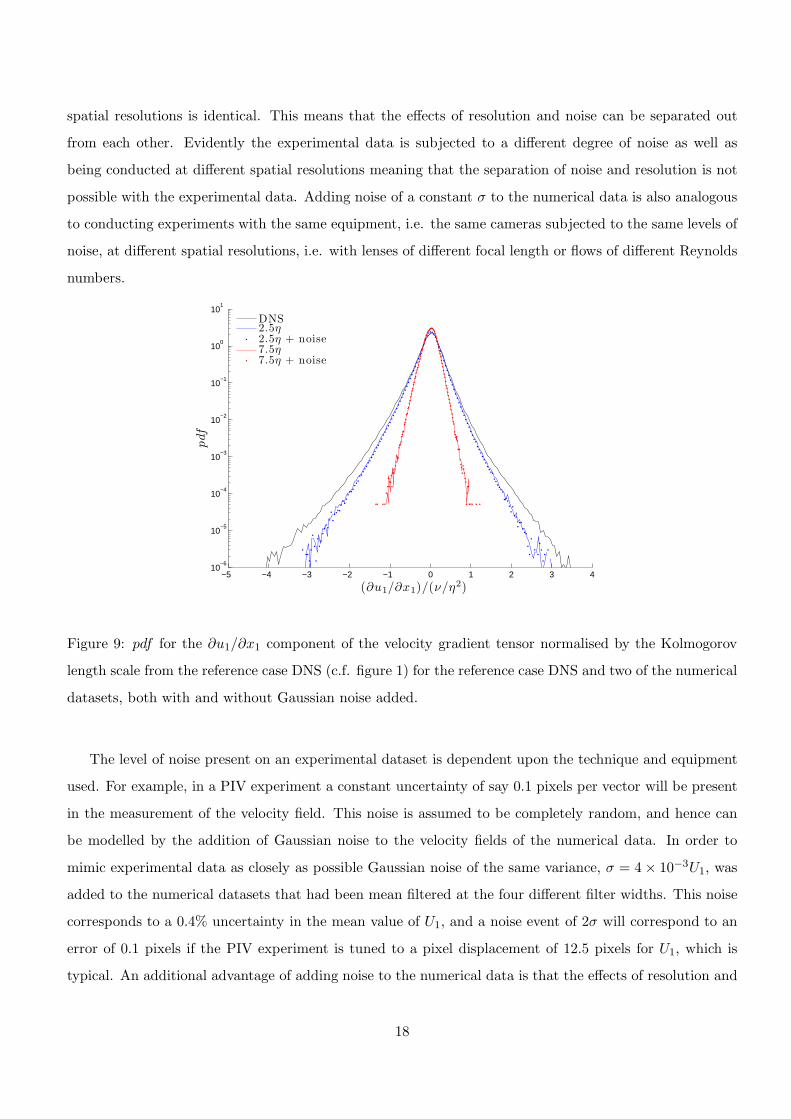
Figure 9: pdf for the ∂u1/∂x1 component of the velocity gradient tensor normalised by the Kolmogorov
length scale from the reference case DNS (c.f. figure 1) for the reference case DNS and two of the numerical
datasets, both with and without Gaussian noise added.
The level of noise present on an experimental dataset is dependent upon the technique and equipment
used. For example, in a PIV experiment a constant uncertainty of say 0.1 pixels per vector will be present
in the measurement of the velocity field. This noise is assumed to be completely random, and hence can
be modelled by the addition of Gaussian noise to the velocity fields of the numerical data. In order to
mimic experimental data as closely as possible Gaussian noise of the same variance, σ = 4 × 10⁻³U1, was
added to the numerical datasets that had been mean filtered at the four different filter widths. This noise
corresponds to a 0.4% uncertainty in the mean value of U1, and a noise event of 2σ will correspond to an
error of 0.1 pixels if the PIV experiment is tuned to a pixel displacement of 12.5 pixels for U1, which is
typical. An additional advantage of adding noise to the numerical data is that the effects of resolution and
18
noise can be separated and discussed separately, which is evidently not possible with experimental data.
Figure 9 shows the pdfs for the ∂u1/∂x1 component of the velocity gradient tensor normalised by the
reference case Kolmogorov length scale, η, as in figure 1. pdfs are shown for the reference case, and the
datasets mean filtered at 2.5η and 7.5η both with and without Gaussian noise added. It can clearly be
seen that the pdfs remain virtually identical for the cases to which noise has and hasn’t been added. This
is repeated in the pdfs for the other components of the velocity gradient, but isn’t shown for brevity.
−1.5 −1 −0.5 0 0.5 1 1.50
0.2
0.4
0.6
0.8
1
s2∗
DNS2.5η2.5η + noise7.5η7.5η + noiseExp.Exp. 6η
(a)
−1.5 −1 −0.5 0 0.5 1 1.50
0.2
0.4
0.6
0.8
1
1.2
1.4
S∗
DNS2.5η2.5η + noise7.5η7.5η + noiseExp.Exp. 6η
(b)
Figure 10: (a) pdf for s2∗ (defined in the text) from the numerical data, experimental data and numerical
data to which Gaussian noise has been added. (b) pdf for S∗ (defined in the text) from the numerical data,
experimental data and numerical data to which Gaussian noise has been added.
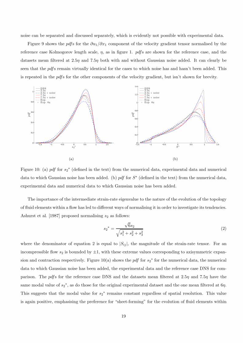
The importance of the intermediate strain-rate eigenvalue to the nature of the evolution of the topology
of fluid elements within a flow has led to different ways of normalising it in order to investigate its tendencies.
Ashurst et al. [1987] proposed normalising s2 as follows:
s2∗ =
√6s2
√
s21+ s2
2+ s2
3
(2)
where the denominator of equation 2 is equal to |Sij |, the magnitude of the strain-rate tensor. For an
incompressible flow s2 is bounded by ±1, with these extreme values corresponding to axisymmetric expan-
sion and contraction respectively. Figure 10(a) shows the pdf for s2∗ for the numerical data, the numerical
data to which Gaussian noise has been added, the experimental data and the reference case DNS for com-
parison. The pdfs for the reference case DNS and the datasets mean filtered at 2.5η and 7.5η have the
same modal value of s2∗, as do those for the original experimental dataset and the one mean filtered at 6η.
This suggests that the modal value for s2∗ remains constant regardless of spatial resolution. This value
is again positive, emphasising the preference for “sheet-forming” for the evolution of fluid elements within
19
the flow. The addition of Gaussian noise, however, reduces the magnitude of the pdf peak and moves it to
a smaller s2∗ value for both the datasets mean filtered at 2.5η and 7.5η. There is a more distinct shift in
the pdf peak for the dataset mean filtered at 2.5η when Gaussian noise is added than that mean filtered at
7.5η. Due to the effect of mean filtering this zero mean noise appears to have a lesser effect on the more
coarsely resolved data.
The addition of Gaussian noise has the effect of introducing a divergence error into the data. This
manifests itself as the tails of the pdfs extending beyond s2∗ = ±1 and the peak value of the pdf decreasing
due to the extended range. This extension of the tails beyond s2∗ = ±1 is also observed on the pdfs
produced from the experimental data, highlighting the divergence error that is inherent in the data due to
experimental noise. Further effects of this divergence error are discussed later.
Lund and Rogers [1994] argued that the normalisation of s2 in equation 2 does not capture the entire
range of strain orientations uniquely and proposed a new normalisation:
S∗ =−3
√6s1s2s3
(s21+ s2
2+ s2
3)3/2
(3)
This new normalisation is again bounded by S∗ = ±1. Figure 10(b) shows probability density functions for
S∗ from the numerical data, the numerical data to which Gaussian noise has been added, the experimental
data and the reference case DNS for comparison. A shift in the location of the modal value of S∗ as
resolution is decreased can be observed in the figure. This is predominantly due to the slight divergence
error that is added to the data as the resolution is coarsened, illustrated by the extension of the tails of
the pdfs from the data mean filtered at 2.5η and 7.5η extending beyond S∗ = ±1. The pdf from the
reference case, and to a lesser extent those from the coarser mean filtered datasets, show the characteristic
shape presented in Lund and Rogers [1994]. However, those created from the experimental datasets and
the numerical datasets to which Gaussian noise has been added differ significantly, with the peak moving
to a value of S∗ somewhat less than one. This was also observed by Lund and Rogers [1994] when noise
was added to their DNS data. The pdfs generated from the two experimental datasets can be seen to
be both qualitatively and quantitatively similar to the noisy numerical datasets, with the tails extending
some way past S∗ = ±1. Ganapathisubramani et al. [2007] argued that this was due to a combination of
experimental divergence error, caused by noise on the data, and a greater degree of uncertainty in lower
magnitude velocity derivatives. It was showed, by means of joint probability density functions between
velocity gradient tensor magnitude and S∗ that this data was reliable, and comparable to DNS datasets
at higher magnitudes of Dij , such as those found in areas of high enstrophy/strain amplification rates.
Figures 10(a) and (b) show that experimental noise has a considerable effect on our observation of
certain kinematic features of shear flow turbulence. One of the effects of this experimental noise is to add
20
an artificial compressibility, ∇ · u 6= 0, to the data, highlighted by the extension of the tails of the pdfs of
figures 10(a) and (b) beyond ±1.
Another kinematic feature of shear flow turbulence that is affected by this artificial compressibility
is the strain - rotation interaction. This interaction and the differences between rotation dominated and
strain dominated regions of the flow can be further examined by looking at the joint probability density
functions between Q and R, the second and third invariants of the velocity gradient tensor respectively.
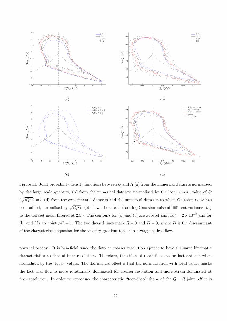
Figure 11 shows joint probability density functions between the second (Q) and third (R) invariants of
the characteristic equation of the velocity gradient tensor for the numerical data normalised by large scale
quantities (a), the “local r.m.s. value of Q” (b) and the experimental data and noisy numerical datasets
(d). Figure 11(c) shows joint pdfs normalised by the large scale quantity constructed from the dataset
mean filtered at 2.5η to which two different levels of noise have been added. The large scale quantity used
to normalise the pdfs of figures 11(a) and (c) is the same as that defined to normalise figure 8. The joint
contour level for the pdfs of figures 11(a) and (c) is 2 × 10⁻³, whereas those for (b) and (d) are both 1.
The dashed lines mark D = 0, where D is the discriminant of the characteristic equation for the velocity
gradient tensor of a divergence free flow and R = 0. The two sectors of the pdf for which D > 0, S1 and S4
in the terminology of Buxton and Ganapathisubramani [2010], are responsible for the bulk of the enstrophy
attenuation (S1: D > 0;R > 0) and enstrophy amplification (S4: D > 0;R < 0). These two sectors are
rotationally dominated regions of the flow (D > 0). It can be seen in figure 11(a) that as the resolution
decreases an increasing proportion of the data is found in these two sectors. Effectively, data is transferred
from the strain dominated regions for which D < 0 to the rotationally dominated regions. In the reference
case DNS sectors S1 and S4 account for 21.3% and 31.3% of the total data points respectively, whereas in
the dataset mean filtered at 7.5η they account for 24.8% and 34.7% respectively. By contrast, the strain
dominated sectors S2 (D < 0;R > 0) and S3 (D < 0;R < 0) account for 36.4% and 11.0% of the reference
DNS case respectively and 30.5% and 10.0% respectively of the dataset mean filtered at 7.5η.
This effect, however, is not observed when the joint pdfs are normalised by the local r.m.s. value for Q
(√
〈Q2〉), as illustrated in figure 11(b). The large scale quantity used to normalise the pdfs of figure 11(a)
is easy to measure experimentally and largely independent of the resolution of the experiment performed,
whereas the r.m.s. value of Q changes (reduces) as the resolution of the experiment is coarsened due to
the mean filtering effect illustrated in figures 1 and 2. The pdfs for all four resolutions show similar shapes
thereby masking the fact that the flow is more rotationally dominated at larger length scales, and more
strain dominated at shorter length scales.
This is of great importance to the experimentalist as the normalisation of these two important quan-
tities by small scale features, such as ηl (“local” Kolmogorov length scale) or√
〈Q2〉 masks an important
21
−6 −4 −2 0 2 4 6 8 10−10
−8
−6
−4
−2
0
2
4
6
R/(Uc/Λf )3
Q/(U
c/Λ
f)2
2.5η5η7.5η15η
(a)
−0.1 −0.05 0 0.05 0.1 0.15 0.2
−0.6
−0.4
−0.2
0
0.2
0.4
R/〈Q2〉3/4
Q/〈Q
2〉1
/2
2.5η5η7.5η15η
(b)
−6 −4 −2 0 2 4 6 8 10−10
−8
−6
−4
−2
0
2
4
6
R/(Uc/Λf )3
Q/(U
c/Λ
f)2
σ/U1 = 0σ/U1 = 0.4%σ/U1 = 1%
(c)
−0.1 −0.05 0 0.05 0.1 0.15 0.2
−0.6
−0.4
−0.2
0
0.2
0.4
R/〈Q2〉3/4
Q/〈Q
2〉1
/2
2.5η + noise5η + noise7.5η + noiseExp.Exp. 6η
(d)
Figure 11: Joint probability density functions between Q and R (a) from the numerical datasets normalised
by the large scale quantity, (b) from the numerical datasets normalised by the local r.m.s. value of Q
(√
〈Q2〉) and (d) from the experimental datasets and the numerical datasets to which Gaussian noise has
been added, normalised by√
〈Q2〉. (c) shows the effect of adding Gaussian noise of different variances (σ)
to the dataset mean filtered at 2.5η. The contours for (a) and (c) are at level joint pdf = 2× 10⁻³ and for
(b) and (d) are joint pdf = 1. The two dashed lines mark R = 0 and D = 0, where D is the discriminant
of the characteristic equation for the velocity gradient tensor in divergence free flow.
physical process. It is beneficial since the data at coarser resolution appear to have the same kinematic
characteristics as that of finer resolution. Therefore, the effect of resolution can be factored out when
normalised by the “local” values. The detrimental effect is that the normalisation with local values masks
the fact that flow is more rotationally dominated for coarser resolution and more strain dominated at
finer resolution. In order to reproduce the characteristic “tear-drop” shape of the Q − R joint pdf it is
22
thus recommended to filter the data to a coarser resolution, in agreement with Worth et al. [2010], and
normalise by a large scale flow quantity.
It can be observed from figure 11(d) that the joint pdfs produced from the experimental datasets are a
different shape to those from the reference DNS dataset and the literature (e.g. Chong et al. [1990]; Perry
and Chong [1994]; Luthi et al. [2009]). There is a significantly reduced strain dominated “Vieillefosse
tail” and a broadening of the rotationally dominated sectors S1 and S4 in the R direction, which is more
pronounced for the coarsely mean filtered experimental dataset than for the original experimental dataset.
This can be explained by the noise, inherent to the PIV process, that is present on the data. The first
invariant of the characteristic equation for the velocity gradient tensor, P = ∇ · u, is not necessarily non-
zero for the experimental data. This divergence error is in line with other similar experimental studies
and is characterised and discussed further in Ganapathisubramani et al. [2007], however it still plays an
important role in shaping the Q − R joint pdf of figure 11. It can be shown that in P − Q − R space the
surface that separates purely real from complex roots, i.e. the discriminant in the three dimensional space,
can be given by [Chong et al., 1990]:
27R2 + (4P 3 − 18PQ)R + (4Q3 − P 2Q2) = 0 (4)
In fully divergence free flow (P = ∇ · u = 0), D can thus be given by:
D = Q3 +27
4R2 (5)
There is thus a discrepancy between the “surface” separating real from complex roots in the P − Q − R
space of not fully divergence free data and the “D = 0” condition separating them in fully divergence free
data and illustrated as the dashed line in figure 11. A two dimensional joint pdf thus becomes insufficient
to characterise the flow according to the invariants of the velocity gradient tensor for a non-divergence
free flow. The joint pdfs between Q and R generated from the noisy numerical datasets are also plotted
on figure 11(d). A similar “fattening” of sectors S1 and S4 and a diminishing of the strain amplification
dominated “Vieillefosse tail” to the experimental datasets is observed for the noisy datasets, indicating that
the Gaussian noise present in experimental data is responsible. Again it can be seen that as the resolution
is coarsened the effect of the noise on the numerical datasets is decreased, as the joint pdfs for the data
mean filtered at 5η and 7.5η to which Gaussian noise has been added look more similar in shape to those
of figures 11(a) and (b), with a more distinct “Vieillefosse tail”. The pdf from the numerical dataset mean
filtered at 2.5η to which noise has been added does, however, closely resemble the experimentally generated
pdfs. This is also in agreement with the PTV study of turbulence under the influence of system rotation
of Kinzel et al. [2010]. Two spatial resolutions are used to produce joint pdfs between Q and R, 2.5η and
23
9.5η. The study reports that as the resolution is coarsened the joint pdf loses its characteristic shape and
more closely resembles that produced from a Gaussian field. Figure 11(c) shows that this is, however, a
noise effect rather than a resolution effect. This figure shows pdfs produced from the dataset mean filtered
at 2.5η to which Gaussian noise has been added with a variance of σ/U1 = 0.4% and σ/U1 = 1%. It
can be seen that the shape of the pdf produced from the dataset to which the highest level of noise has
been added is unrecognisable from those of figure 11(a), and closely resembles that of a Gaussian random
variable and that of the coarsely resolved case in Kinzel et al. [2010]. However, the joint pdf produced
from the dataset mean filtered at 15η (≈ 10ηl) in figure 11(a) retains the characteristic “tear-drop” shape.
Further joint pdfs were produced between Q and R for the more coarsely mean filtered datasets to which
this higher level of noise has been added, but they are not shown for brevity. These confirm the finding
that Gaussian noise has a diminishing effect on the shape of these pdfs as spatial resolution is coarsened.
Equation 1 shows that as ∆x is increased, i.e. resolution is coarsened, the velocity gradients decrease in
magnitude. Thus Gaussian noise of identical variance will reduce the magnitudes of the divergence error,
∇ · u, present on the data and hence the behaviour of the velocity gradient tensor’s invariants.
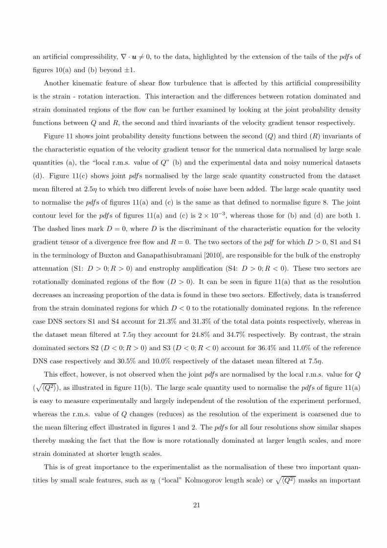
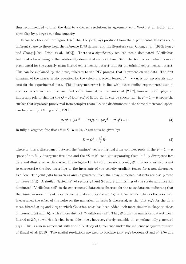
(a) (b) (c)
Figure 12: (a) Slice located at P/(ν/η2) = −0.25 illustrating contours of the three dimensional joint
probability density function between P , Q and R from the experimental dataset. (b) Slice located at
P/(ν/η2) = 0 for the three dimensional joint pdf . The contour in black represents the contour level of the
joint pdf = 30 of the experimental data of figure 11(d). (c) Slice located at P/(ν/η2) = 0.25 for the three
dimensional joint pdf .
The effect of this Gaussian noise introduced divergence error on the experimental data is illustrated in
figure 12. The figure shows three slices, located at P/(ν/η2) = −0.25, 0 and 0.25 respectively of the three
dimensional joint probability density function between P , Q and R for the experimental dataset with the
two dimensional Q − R pdf of figure 11(d) superimposed as the black line. It can immediately be seen
24
(a) (b) (c)
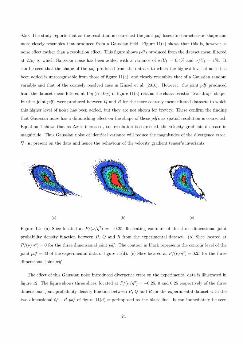
(d) (e) (f)
Figure 13: Slices located at P/(ν/ηl2) = −0.15 (a), P/(ν/ηl
2) = 0 (b) and P/(ν/ηl2) = 0.15 (c) for
the three dimensional joint pdf between P , Q and R for the numerical dataset mean filtered at 2.5η to
which Gaussian noise of variance σ/U1 = 0.4% has been added. (d), (e) and (f) show slices located at
P/(ν/ηl2) = −0.15, P/(ν/ηl
2) = 0 and P/(ν/ηl2) = 0.15 respectively for the P −Q−R 3D joint pdf for the
numerical dataset mean filtered at 2.5η to which Gaussian noise of variance σ/U1 = 1% has been added.
The contour in black represents the joint pdfs between Q and R from figure 11(c) for the two different
noise levels.
that the shape of the three dimensional joint pdf at P = 0, i.e. where the divergence free criteria is met,
is very similar to those of the numerical datasets of figure 11(a), with a clear “Vieillefosse tail” evident.
Figures 12(a) and (c) are presented to illustrate the effect of artificial compressibility, i.e. ∇·u 6= 0, that is
introduced into the data by means of intrinsic experimental errors. It can be seen that the three dimensional
pdf is not symmetric about P = 0, with regions of negative P tending to increase the contribution of sector
S4 (relative to the divergence free case) and regions of positive P tending to increase the contribution of
sector S1. Both P < 0 and P > 0 have the effect of reducing the “Vieillefosse tail”, with respect to the
divergence free case, and thus the joint pdf between Q and R of figure 11 has a much greater proportion
25
of swirling data points (sector S1 accounts for 29% and S4 accounts for 37% of the total data points).
The fact that the three dimensional joint pdf is not symmetrical about P = 0 is explained by the
nature of the artificial compressibility “added” to the flow by the experimental error. When P is positive,
i.e. ∇ · u > 0, this compressibility corresponds to a negative “density gradient” (∇ · ρ < 0) which is
representative of a compressible flow in a favourable pressure gradient in which waves travelling through
the fluid diverge. When P is negative this corresponds to a positive “density gradient” (∇ · ρ > 0) which
is representative of a compressible flow in an adverse pressure gradient in which waves travelling through
the fluid coalesce (into a shock if the Mach number is greater than 1). These are thus two different
physical processes and account for the asymmetry in the three dimensional joint pdf . This is in agreement
with the study of Pirozzoli and Grasso [2004], examining the effect of compressibility on turbulence. As
spatial resolution is coarsened the divergence error of a dataset will increase. This is also evident in the
joint pdfs of figure 11(a) for the mean filtered datasets which show an increase in relative contributions
of sectors S1 and S4 (relative the reference DNS case) and in figure 10. Three dimensional joint pdfs
between P , Q and R, which are not shown for brevity, suggest that there is a slight increase in the level
of artificial compressibility introduced into these coarser datasets. This increases the relative importance
of rotationally dominated regions of the flow, thereby increasing the distance over which these regions are
spatially correlated, as visualised in figure 6.
The above observation is supported by the similar three dimensional joint pdf between P , Q and R
of figure 13, formed from the well resolved (2.5η) but noisy DNS dataset. Figures 13(a), (b) and (c)
again illustrate a slice of the joint pdf located at P/(ν/η2) = −0.15, 0 and 0.15 respectively formed from
the numerical dataset to which Gaussian noise of σ/U1 = 0.4% has been added. This again shows the
“Vieillefosse tail” at P = 0 and the relative increase in the importance of sector S4 for negative values
of P and sector S1 for positive values of P . These same trends are also illustrated in figures 13(d), (e)
and (f) which show the three dimensional joint pdf formed from the dataset mean filtered at 2.5η to
which the higher noise level of σ/U1 = 1% has been added, although it is obviously noisier. The artificial
compressibility of experimental data thus increases the sector of Q − R space that is largely responsible
for enstrophy amplification (S1) and reduces the contribution of the strain amplifying “Vieillefosse tail”
thereby affecting the balance between these two terms which is of great importance to the dynamics of
dissipation.
The interaction between strain and rotation is often examined by observation of the alignment between
the eigenvectors of the strain-rate tensor and the vorticity vector. Figure 14 shows the pdfs for the
magnitude of the alignment cosine between the vorticity vector and the extensive strain-rate eigenvector (a),
intermediate strain-rate eigenvector (b) and the compressive strain-rate eigenvector (c). All of the figures
26

0 0.1 0.2 0.3 0.4 0.5 0.6 0.7 0.8 0.9 10.85
0.9
0.95
1
1.05
1.1
1.15
1.2
1.25
1.3
| ~e1 · ~ω|
DNS2.5η2.5η + noise7.5η7.5η + noiseExp.Exp. 6η
(a)
0 0.1 0.2 0.3 0.4 0.5 0.6 0.7 0.8 0.9 1
0.8
1
1.2
1.4
1.6
1.8
2
2.2
| ~e2 · ~ω|
DNS2.5η2.5η + noise7.5η7.5η + noiseExp.Exp. 6η
(b)
0 0.1 0.2 0.3 0.4 0.5 0.6 0.7 0.8 0.9 1
0.7
0.8
0.9
1
1.1
1.2
1.3
1.4
1.5
| ~e3 · ~ω|
DNS2.5η2.5η + noise7.5η7.5η + noiseExp.Exp. 6η
(c)
Figure 14: pdfs of magnitude of alignment cosine between the eigenframe of the strain-rate tensor ((a)
extensive eigenvector, (b) intermediate eigenvector and (c) compressive eigenvector) and the vorticity
vector. The pdfs are constructed using the numerical datasets, numerical datasets to which Gaussian noise
has been added and the experimental datasets.
show pdfs produced from the numerical data, both with and without noise added and the experimental
data with the reference case DNS also plotted for comparison. The pdfs from the reference case show the
extensively reported arbitrary alignment between e1 and ω and the preferential perpendicular e3 - ω and
parallel e1 - ω alignments. There can be seen to be a slight resolution effect to the observation of these
alignments. The datasets mean filtered at 2.5η and 7.5η show a slight tendency for e1 to become aligned
in parallel with ω as resolution is coarsened coupled to a slight reduction in the preference in parallel
alignment between e2 and ω.
There is no notable resolution effect to the alignment between e3 and ω. The addition of Gaussian
27
noise is observed to have a much more significant effect by observing the pdfs constructed from the mean
filtered numerical datasets to which noise has been added. All three figures again show that the addition of
noise is more significant to the more finely resolved (2.5η) dataset than the coarser one (7.5η). In general
noise can be seen to make the alignment between all three eigenvectors and ω more arbitrary, i.e. “flatten”
the pdfs. This does not appear to be the case for the experimental data, however. The fact that the
addition of noise has a greater effect on the more finely resolved data is again a result of the amplification
of the noise on the velocity field in the velocity gradients due to the smaller ∆x in equation 1.
4 Conclusions and further discussion
A direct numerical solution is performed for a nominally two dimensional planar mixing layer and then
mean filtered onto a regular Cartesian gird at four different spatial resolutions, namely 2.5η, 5η, 7.5η and
15η. This data, at different spatial resolutions, is then directly compared to the original DNS dataset and
stereoscopic cinematographic PIV data from Ganapathisubramani et al. [2007] in order to examine the
effect of spatial resolution on the kinematic fine scale features that affect the strain - rotation interaction
in shear flow turbulence. The experimental data is also mean filtered from an original resolution of 3η to
a new coarser resolution of 6η.
The first important effect of reducing spatial resolution is the reduction of the magnitudes of the
components of the velocity gradient tensor due to mean spatial filtering. The exponential tails to the
pdfs of the components of Dij , as reported by Sreenivasan and Antonia [1997]; Ganapathisubramani et al.
[2008] amongst others, is only visible at coarser resolutions of 3η (the experimental resolution) and above.
For the more finely resolved data the gradients of these pdfs are not linear in semi-logarithmic coordinates
but decreases at the high magnitude events. This spatial mean filtering has the effect of reducing the
intermittency of the dissipation and enstrophy, the scalar analogues to strain and rotation respectively.
Fine scale turbulence is by its very nature an intermittent phenomenon and this intermittency has been
shown to be extremely important to the rate of enstrophy amplification (ωiSijωj). “Extreme events”, those
that are up to a thousand time the r.m.s. value and constitute the long tails of the pdfs such as figure 3, are
responsible for a greatly disproportionate amount of the overall enstrophy amplification. It is found that
coarser resolution has an almost equal effect on the reduction of intermittency of enstrophy (rotation) and
dissipation (strain). This is despite the fact that dissipation is shown to be spatially coherent over greater
length scales and in two dimensions as opposed to one; high enstrophy events are known to form “worms”
(e.g. Jimenez et al. [1993]) which are spatially coherent only in one dimension, whereas high dissipation
events are known to form “sheets” which have a high spatial coherence in two dimensions.
28
In agreement with the experimental findings from the tomographic PIV study of Worth [2010] the
length scale over which high dissipation events and high enstrophy events are spatially coherent is found to
be a constant number of discrete grid points, regardless of the resolution of the grid. This suggests that the
length scales of dissipation and enstrophy follow the filter that has been imposed upon them. This leads to
these length scales becoming larger in physical units, as the resolution is coarsened. This is still the case,
albeit to a lesser extent, when the characteristic length scales of these experiments are normalised by fine
scale quantities that are calculated from the data itself. Thus the growth of these structures as resolution
is coarsened is diminished with respect to fine scale flow quantities in comparison to fixed, large scale
quantities. Worth et al. [2010] suggested that the minimum resolution required to confidently determine
these length scales is 3η, the distance at which noise-related over prediction balances the spatial averaging
under prediction of the spatial gradients. The comparison between the “best case” DNS and the data mean
filtered at 2.5η and the experimental data (3η) suggests that even greater resolution may be required for
a confident prediction. The fact that the experimental data of figure 3 falls between the DNS data mean
filtered at 2.5η and 5η suggests that predictions as to the “real flow” may be made from under resolved
data.
The eigenvalues of the rate of strain tensor, Sij , determine the nature of the strain that a fluid element
within the flow is subjected to. It has been shown that decreasing spatial resolution effects the extreme
strain-rates far more than the more frequently occurring, modal events. The location of the peak/mode
of the pdfs for all three principal strain-rates is observed to remain at the same location as resolution
is decreased, in both the experimental jet flow and the numerical mixing layer, whereas the tails become
narrower when normalised by large scale quantities. This suggests that the extreme strain-rates are spatially
coherent over only small distances, whereas the modal events are spatially coherent over much greater
length scales. Again, however, when these quantities are normalised by fine scale quantities calculated
from the data itself there is a variance in the modal values of these strain-rates. Both the jet flow and
mixing layer data show the same location for the modal value of the intermediate strain-rate eigenvalue
at s2 ≈ 0.04ν/ηl2. This positive value reveals that shear flow turbulence has a preference for “sheet-
forming”, as opposed to “tube-forming”, topological evolution of fluid elements as a positive intermediate
strain-rate means a fluid element is subjected to two orthogonal extensive strains and a further orthogonal
compression, resulting in a tendency to extend in-plane and flatten out of plane.
Another consequence of calculating spatial gradients from coarsely resolved data is that the divergence
free condition (∇ · u = 0) vanishes and a divergence error is introduced into the data. This problem is
exacerbated by noise introduced by experimental error [Ganapathisubramani et al., 2007]. The effect of
the introduction of a divergence error is to increase the importance of rotationally dominated regions of
29
the flow, ones for which the characteristic equation for the velocity gradient tensor has complex roots, at
the expense of the strain dominated regions of the flow (real roots only). This is observed particularly in
figure 12 which illustrates the effect of the artificial compressibility on the joint pdf between the second
(Q) and third (R) invariants of the characteristic equation for the velocity gradient tensor generated from
the original experimental dataset. This artificial compressibility is asymmetric about P = ∇ · u = 0, with
P < 0 increasing the relative contribution of sector S4 (D > 0;R < 0) and P > 0 increasing the relative
contribution of sector S1 (D > 0;R > 0). This behaviour is also observed in figure 13 which is generated
from the numerical data to which Gaussian noise has been added to mirror the noise generated by the
experimental process. Gaussian noise with a constant value of σ = 0.4% of U1 was added to the numerical
data at different spatial resolutions. It was observed that Gaussian noise has a decreasing effect on the joint
pdfs between Q and R as spatial resolution is coarsened, as a consequence of ∆x, from equation 1 increasing
whilst√
〈u′
noise
2〉 remains constant. An increase in the divergence error, either by the introduction of
experimentally generated Gaussian noise or by a coarse spatial resolution also has a substantial effect on
the dynamics of dissipation. The relative contribution of the strongly enstrophy amplifying sector S4 in
Q−R space is increased, whereas the strain amplifying “Vieillefosse tail” is diminished, thereby upsetting
the balance of the source and sink terms for the dynamics of dissipation and skewing our observation of
the strain - rotation interaction in shear flow turbulence.
A further distortion of our observation of the strain - rotation interaction due to the presence of
experimental noise is also present in the alignment pdfs between the eigenvectors of the rate of strain
tensor and the vorticity vector presented in figure 14. These show that there is a minor resolution effect
in our observation of these alignments, the most important of which is the slight preference for ω to be
aligned in parallel with e1, at the expense of e2. The effect of experimental noise is shown to be of greater
significance than that of resolution. Noise is shown to make all three of the alignments more arbitrary and
less pronounced.
The authors would like to thank EPSRC for providing the computing resources on HECToR through
the Resource Allocation Panel and for funding the experimental research through Grant No. EP/F056206.
Funding from the Royal Aeronautics Society for ORHB is also greatly appreciated.
References
W.T. Ashurst, A.R. Kerstein, R.M. Kerr, and C.H. Gibson. Alignment of vorticity and scalar gradient
with strain rate in simulated Navier-Stokes turbulence. Phys. Fluids, 30:2343–2353, 1987.
30
I. Bermejo-Moreno, D.I. Pullin, and K. Horiuti. Geometry of enstrophy and dissipation, resolution effects
and proximity issues in turbulence. J. Fluid Mech., 620:121–166, 2009.
O.R.H. Buxton and B. Ganapathisubramani. Amplification of enstrophy in the far field of an axisymmetric
turbulent jet. J. Fluid Mech., 651:483–502, 2010.
M.S. Chong, A.E. Perry, and B.J. Cantwell. A general classification of three-dimensional flow fields. Phys.
Fluids A, 2(5):765–777, 1990.
K.T. Christensen. The influence of peak-locking errors on turbulence statistics computed from PIV en-
sembles. Exp. Fluids, 36:484–497, 2004.
K.T. Christensen and R.J. Adrian. Measurement of instantaneous Eulerian acceleration fields by particle
image accelerometry: method and accuracy. Exp. Fluids, 33:759–769, 2002.
D.A. Donzis, P.K. Yeung, and K.R. Sreenivasan. Dissipation and enstrophy in isotropic turbulence: Res-
olution effects and scaling in direct numerical simulations. Phys. Fluids, 20(045108):1–16, 2008.
B. Ganapathisubramani, E.K. Longmire, I. Marusic, and S. Pothos. Dual-plane PIV technique to determine
the complete velocity gradient tensor in a turbulent boundary layer. Exp. Fluids, 39(2):222–231, 2005.
B. Ganapathisubramani, K. Lakshminarasimhan, and N.T. Clemens. Determination of complete velocity
gradient tensor by using cinematographic stereoscopic PIV in a turbulent jet. Exp. Fluids, 42:923–939,
2007.
B. Ganapathisubramani, K. Lakshminarasimhan, and N.T. Clemens. Investigation of three-dimensional
structure of fine-scales in a turbulent jet by using cinematographic stereoscopic PIV. J. Fluid Mech.,
598:141–175, 2008.
J. Jimenez, A.A. Wray, P.G. Saffman, and R.S. Rogallo. The structure of intense vorticity in isotropic
turbulence. J. Fluid Mech., 255:65–90, 1993.
R.M. Kerr. Higher-order derivative correlations and the alignment of small-scale structures in isotropic
numerical turbulence. J. Fluid Mech., 153:31–58, 1985.
M. Kinzel, M. Wolf, M. Holzner, B. Luthi, C. Tropea, and W. Kinzelbach. Simultaneous two-scale 3D-
PTV measurements in turbulence under the influence of system rotation. Exp. Fluids, pages 1–8, 2010.
10.1007/s00348-010-1026-6.
31
S. Laizet and E. Lamballais. High-order compact schemes for incompressible flows: A simple and efficient
method with quasi-spectral accuracy. J. Comp. Phys., 228(16):5989–6015, 2009.
S. Laizet, S. Lardeau, and E. Lamballais. Direct numerical simulation of a mixing layer downstream a
thick splitter plate. Phys. Fluids, 22(015104):1–15, 2010.
P. Lavoie, G. Avallone, F. De Gregorio, G.P. Romano, and R.A Antonia. Spatial resolution of PIV for the
measurement of turbulence. Exp. Fluids, 43(1):39–51, 2007.
T.S. Lund and M.M. Rogers. An improved measure of strain state probability in turbulent flows. Phys.
Fluids, 6(5):1838–1847, 1994.
B. Luthi, A. Tsinober, and W. Kinzelbach. Lagrangian measurement of vorticity dynamics in turbulent
flow. J. Fluid Mech., 528:87–118, 2005.
B. Luthi, M. Holzner, and A. Tsinober. Expanding the Q − R space to three dimensions. J. Fluid Mech.,
641:497–507, 2009.
J.A. Mullin and W.J.A. Dahm. Dual-plane stereo particle image velocimetry measurements of velocity
gradient tensor fields in turbulent shear flow II. Experimental results. Phys. Fluids, 18(035102):1–28,
2006.
A.E. Perry and M.S. Chong. Topology of flow patterns in vortex motions and turbulence. Appl. Sci. Res.,
53:357–374, 1994.
S. Pirozzoli and F. Grasso. Direct numerical simulation of isotropic compressible turbulence: Influence of
compressibility on dynamics and structures. Phys. Fluids, 16(12):4386–4407, 2004.
G.R. Ruetsch and M.R. Maxey. Small-scale features of vorticity and passive scalar fields in homogeneous
isotropic turbulence. Phys. Fluids A, 3(6):1587–1597, 1991.
K.R. Sreenivasan and R.A. Antonia. The phenomenology of small-scale turbulence. Annu. Rev. Fluid
Mech., 29:435–472, 1997.
B. Tao, J. Katz, and C. Meneveau. Geometry and scale relationships in high Reynolds number turbulence
determined from three-dimensional holographic velocimetry. Phys. Fluids, 12(5):941–944, 2000.
B. Tao, J. Katz, and C. Meneveau. Statistical geometry of subgrid-scale stresses determined from holo-
graphic particle image velocimetry measurements. J. Fluid Mech., 457:35–78, 2002.
G.I. Taylor. Statistical theory of turbulence. Proc. R. Soc. Lond. A, 151(873):421–444, 1935.
32
H. Tennekes and J.L. Lumley. A first course in turbulence. MIT Press, 1972.
A. Tsinober. Is concentrated vorticity that important? Eur. J. Mech B/Fluids, 17(4):421–449, 1998.
A. Tsinober, E. Kit, and T. Dracos. Experimental investigation of the field of velocity gradients in turbulent
flows. J. Fluid Mech., 242:169–192, 1992.
F. van der Bos, B. Tao, C. Meneveau, and J. Katz. Effects of small-scale turbulent motions on the filtered
velocity gradient tensor as deduced from holographic particle image velocimetry measurements. Phys.
Fluids, 14(7):2456–2474, 2002.
P. Vieillefosse. Local interaction between vorticity and shear in a perfect incompressible fluid. J. Phys.,
43(6):837–842, 1982.
A. Vincent and M. Meneguzzi. The dynamics of vorticity tubes in homogeneous turbulence. J. Fluid
Mech., 258:245–254, 1994.
P. Vukoslavcevic, J.M. Wallace, and J.L. Balint. The velocity and vorticity vrctor fields of a turbulent
boundary layer. Part 1. Simultaneous measurement by hot-wire anemometry. J. Fluid Mech., 228:25–51,
1991.
J.M. Wallace and P. Vukoslavcevic. Measurement of the velocity gradient tensor in turbulent flows. Annu.
Rev. Fluid Mech., 42:157–181, 2010.
J. Westerweel. Theoretical analysis on the measurement precision in particle image velocimetry. Exp.
Fluids [Suppl.], 29:S3–S12, 2000.
N.A. Worth. Tomographic-PIV Measurement of Coherent Dissipation Scale Structures. PhD thesis, Cam-
bridge University, 2010.
N.A. Worth, T.B. Nickels, and N. Swaminathan. A tomographic PIV resolution study based on homoge-
neous isotropic turbulence DNS data. Exp. Fluids, 49(3):637–656, 2010.
33