J Econ Growth (2017) 22:1–33DOI 10.1007/s10887-016-9137-4

The effect of aid on growth: evidence froma Quasi-experiment

Sebastian Galiani1 · Stephen Knack2 ·Lixin Colin Xu2 · Ben Zou3

Published online: 2 September 2016© Springer Science+Business Media New York 2016

Abstract The literature on aid and growth has not found a convincing instrumental variableto identify the causal effects of aid. This paper exploits an instrumental variable based onthe fact that, since 1987, eligibility for aid from the International Development Association(IDA) has been based partly on whether or not a country is below a certain threshold ofper capita income. The paper finds evidence that other donors tend to reinforce rather thancompensate for reductions in IDA aid following threshold crossings. Overall, aid as a share ofgross national income (GNI) drops about 59% on average after countries cross the threshold.Focusing on the 35 countries that have crossed the income threshold frombelowbetween1987and 2010, a positive, statistically significant, and economically sizable effect of aid on growthis found. A 1 percentage point increase in the aid to GNI ratio from the sample mean raises

We are grateful for valuable comments by several anonymous referees, George Clarke, Michael Clemens,Yingyao Hu, Aart Kraay, Martin Ravallion, and seminar participants at the 2013 Southern EconomicsAssociation Annual Meeting, the University of Toronto, Xiamen University, and the Center for GlobalDevelopment.

Electronic supplementary material The online version of this article (doi:10.1007/s10887-016-9137-4)contains supplementary material, which is available to authorized users.

B Stephen Knacksknack@worldbank.org

Sebastian Galianigaliani@econ.umd.edu

Lixin Colin Xulxu1@worldbank.org

Ben Zoubenzou@msu.edu

1 Department of Economics, University of Maryland, and NBER, College Park, MD 20742, USA

2 World Bank – Development Research Group, 1818 H Street, N.W., Washington, DC 20433, USA

3 Department of Economics, Michigan State University, East Lansing, MI 48824, USA

123

2 J Econ Growth (2017) 22:1–33

annual real per capita growth in gross domestic product by approximately 0.35 percentagepoints.

Keywords Aid effectiveness · Growth · Causal effect and Quasi-experiment

JEL Classification O1 · O4

1 Introduction

Whether foreign aid causes economic growth in recipient countries is a highly debatedresearch question. Identification of the causal effect of aid on growth has been elusive so fardue to the endogeneity of aid in growthmodels. An instrumental variable is needed to addressthese problems. However, as Clemens et al. (2012) conclude in their recent assessment: “theaid-growth literature does not currently possess a strong and patently valid instrumentalvariable with which to reliably test the hypothesis that aid strictly causes growth.”

In this paper we contribute to this literature by instrumenting, in an economic growthequation, the endogenous aid variable exploiting a plausible quasi-experiment created by theincome threshold set by IDA (International Development Association), the World Bank’sprogram of grants and concessionary loans to low-income countries. We exploit this newinstrument to investigate the causal effect of aid on growth.

This income threshold has been used as a key criterion in allocating scarce IDA resourcessince 1987, and is adjusted annually only to take into account inflation. Other major donorsalso appear to use the IDA threshold as an informative signal about where developmentaid is most needed, and we show that total aid declines significantly once a recipient coun-try crosses the IDA income threshold from below. The IDA threshold is nevertheless anarbitrary income level that does not necessarily represent any structural change in eco-nomic growth. Threshold crossing is thus a plausibly valid instrumental variable for aidover time for a recipient country in a panel data model that controls for initial incomelevels and also includes country and period effects (we group years into 8 three-yearperiods).

The main concern with successfully identifying an internally consistent estimate is thatsome countries might cross the threshold by experiencing a series of large positive shocksthat are eventually reversed, making the exclusion restriction invalid. We argue that thisconcern is largely misplaced. On average, our sample of countries grew faster after crossingthe IDA threshold than before, consistent with the fact that developing countries in generalexhibited better performance in the latter part of our 1987-2010 sample period. Moreover,our empirical growth model accounts for the differential timing at which countries crossthe IDA threshold. In our analysis we exploit only the data for the countries that cross thethreshold from below during the period studied while our growth model allows countriesto grow at different rates over time (by allowing for country-specific effects on growth andby allowing conditional convergence). Additionally, countries start at the beginning of thesample period from different levels below the threshold. Hence, the differential timing atwhich countries cross the IDA threshold from below exploited for identification in our studydoes not have to be driven by unobservable shocks.1 We further investigate this threat to ouridentification strategy by implementing a battery of tests and robustness checks. In particular,

1 This assertion applies to countries crossing from below, but perhaps not to the smaller set of countriescrossing the threshold from above; at least they display systematic negative growth rates. Moreover, IDApolicies are premised on the expectation of growth and eventual graduation, and instances of crossing the

123

J Econ Growth (2017) 22:1–33 3

we fail to reject the null hypothesis of no serial autocorrelation in the error term of the modelimplied by the threat to the validity of our instrument posed above. We also show that resultsare robust to controlling for one and two period lags of growth, which would not be thecase if the country receives a transitory positive shock around the time of crossing whichis eventually reversed. Importantly, we use an alternative instrumental variable based on asmoothed income trajectory which is unaffected by country specific idiosyncratic shocksand obtain similar results. All in all, these and other robustness checks do not point towardrejecting our identification strategy.

Using a sample of 35 countries that crossed the IDA threshold from below between 1987and 2010, we find that a 1% increase in the aid to GNI ratio raises the annual real per capitashort term GDP growth rate by 0.031 percentage points. The mean aid to GNI ratio at thecrossing is 0.09, so a 1 percentage point increase in the aid to GNI ratio raises annual real percapita GDP growth by approximately 0.35 percentage points. This effect is about 1.75 timesas large as those reported by Clemens et al. (2012). Using OLS with fixed effects and laggingaid by a period, they find that a one percentage point increase in aid/GDP (at aid levels similarto our sample mean) is followed by at most a 0.2 percentage-point increase in growth of realGDP per capita.We find similar-sized effects in our sample, without instrumenting for aid butmerely lagging it by a period and including fixed effects. We also present evidence consistentwith the possibility that OLS estimates suffer from attenuation bias due to measurementerror in aid, which is exacerbated when the variability in the aid to GNI ratios is exploitedto identify the effect of aid on growth in a fixed effects or first-differenced growth equationcommonly used in the literature. Thus, one should expect that a valid 2SLS produces largerestimates than OLS. Naturally, this could also be the case if growth affects aid levels.

The sizable effect of aid on growth we find may be attributable in part to the fact that oursample consists of low-income countries that successfully crossed the IDA threshold at somepoint between 1987 and 2010. Aid may have been more effective in these countries–e.g.due to better economic policies and lower corruption—than in countries remaining belowthe threshold. Relative to middle-income countries, countries in our sample likely face morestringent financial constraints, which again should make aid effects stronger. Furthermore,it is possible that reductions in aid after crossing the IDA threshold may have a larger neg-ative effect on growth than any positive effects from aid increases, due to adjustment costs.We provide suggestive evidence, however, that our results might have meaningful externalvalidity to the remaining poor countries as they grow closer to the IDA threshold.

A back-of-the-envelope calculation based on a simple growthmodel and the coefficient onaid in investment regressions suggests that investment could be an important channel throughwhich aid affects growth. We show that the investment rate drops following the reductionin aid. Increasing the aid to GNI ratio by 1 percentage point increases the investment toGDP ratio by 0.54 percentage points, although this coefficient is generally not significant.The magnitude of the effects on growth and investment is consistent with the average capitalstock to GDP ratio for the sample countries, which we estimate to be approximately two.

As in most of the literature relying on panel data covering a short period of time, weestimate the short-run effect of aid on growth, an effect that mainly operates through physical

threshold from above are dealt with in a more ad hoc fashion. In such cases, IDA has often been “reluctant toaccept renewed claims on its scarce concessional resources, especially if this would reward poor performance”(Kapur et al. 1997). Crossing from above and from below may therefore have highly asymmetric effects onaid, and in turn on subsequent growth. In particular, crossing from above would likely be a weaker instrument(Footnote 1 continued)for aid, and its effects would be less precisely estimated due to the smaller sample of relevant countries. Wetherefore focus only on the countries that cross the IDA threshold from below.

123

4 J Econ Growth (2017) 22:1–33

investment. In the long run, aid could affect growth through several other channels, butits identification requires exogenous changes in aid over a very long period of time. Ourinstrument does not provide such exogenous variability to estimate that parameter.2

The rest of the paper is organized as follows. Section 2 briefly reviews past studies testingthe causal effect of aid on growth. Section 3 describes the data and the sample. Section 4presents the effect of IDA threshold-crossing on the volume of aid received. Section 5 presentsthe empirical model and the baseline results. Section 6 explores somemechanisms and Sect. 7discusses the external validity of our results. Section 8 concludes.

2 Previous aid-growth studies

Following the influential studies by Boone (1996) and Burnside and Dollar (2000), manyothers have emerged, but a basic consensus is still absent. Easterly et al. (2004) show that thekey finding of Burnside and Dollar (2000)—namely that aid contributes to growth but onlywhere economic policies are favorable—is not robust to the use of an updated and enlargeddataset. Rajan and Subramanian (2008) and Arndt et al. (2010), are only two of many recentpapers that review the bulk of the existing literature yet arrive at differing conclusions.3

Identifying the causal effect of aid on growth is fraught with difficulties. First, aid relativeto GNI is likely measured with error. The problem of measurement error is exacerbated asthe estimated model is often demeaned or first differenced to eliminate the country fixedeffects. Second, identification might be confounded by unobserved factors that determineboth economic growth and aid. Third, growth itself could also affect aid. In response tothese potential problems, previous studies have introduced different instrumental variablesto identify the causal effect of aid on growth. In this section we briefly review the majoridentification strategies exploited in the literature.

Studies using cross-sectional data often rely on population size, economic policies anddonor-recipient political connections as instruments for aid (e.g., Boone 1996; Burnsideand Dollar 2000; Rajan and Subramanian 2008). These instruments are likely to violate theexclusion restriction, as they are correlated with observable and plausibly also unobservedcountry-level characteristics that also contribute to growth (Hansen and Tarp 2001). Forexample, population size can affect economic growth through channels other than aid (Bazziand Clemens 2013). Donor-recipient ties (e.g. colonization, trade or migration) that are cor-related with aid flows can also affect growth indirectly through the institutional environment(Acemoglu et al. 2001) or other channels.

Other studies relying on panel data control for time-invariant determinants of growth byfirst differencing the data or by conditioning on country fixed effects. These studies focusmainly on the short term effect of aid on growth. Many such studies adopt a dynamic panelmodel and employ difference or system GMM estimators, instrumenting for current aid withlagged values of income and aid, and with other standard cross-country regressors (e.g.,Hansen and Tarp 2001; Rajan and Subramanian 2008). However, recent studies show thatGMMestimators of dynamic panel models using all mechanical instruments are unstable andpotentially severely biased infinite samples, due to the problemofmany andweak instruments(Roodman 2007, 2009a, b; Bazzi and Clemens 2013; Bun and Windmeijer 2010). System

2 Regressing the average growth rate over a long period of time on the average aid in that period does notidentify the long-term effect of aid on economic growth, even if aid were exogenous in that equation.3 Also see Temple (2010) and Qian (2015) for two comprehensive reviews of theory, evidence, and practiceof foreign aid.

123

J Econ Growth (2017) 22:1–33 5

GMM estimators, in addition, use additional instruments and require additional assumptionson exclusion restrictions.

Sharing the spirit of our paper, several recent studies exploit donor-recipient connectionsinteracted with over-time variations in total donor contributions. Werker et al. (2009) instru-ment for aid with the interaction between the price of oil and a dummy for whether recipientcountries are Muslim, and find a small and marginally significant effect of lagged aid ongrowth using annual data. However, using four-year period averages, they find no significanteffect of (contemporaneous) aid on growth. Nunn and Qian (2014) find that humanitarianaid extends civil war, using variation over time in U.S. wheat harvests to instrument for theamount of humanitarian aid that a country receives. Temple and Van de Sijpe (2014) find thataid increases net imports and total consumption (both as shares of GDP) by constructing asyntheticmeasure of aid by taking each recipient country’s share of aid in a donor’s aid budgetin an initial period and multiplying it by the donor’s total aid budget in the current period.Dreher and Langlotz (2015) use the interaction between donor government fractionalization(by party) and a recipient government’s probability of receiving aid from the donor to instru-ment for aid, and find no significant effect of it on growth. Channing et al. (2015) review arange of aid-growth studies published since 2008 that attempt to address the endogeneity ofaid in various ways (e.g.. Clemens et al. 2012; Bruckner 2013), and conclude that “the largemajority…have found positive impacts,” particularly when effects are assessed over longertime periods. While these papers rely mostly on historical relationships between bilateraldonors and recipients or natural shocks in grain outputs, we adopt a different identificationstrategy, exploiting a natural experiment based on declines in aid after developing countriessurpass a pre-determined level of GNI per capita. Because instrumental variable-based esti-mates reflect local average treatment effects for the complier group (Angrist et al. 1996),our identification strategy only identifies the effect for low-income countries that experiencechanges in aid after crossing the IDA graduation threshold.

3 Data and sample

The data for this study are primarily from two sources. Income, investment, economic growth,and other country characteristics are from the World Bank’s World Development Indica-tors (WDI).4 Aid data are obtained from the OECD’s Development Assistance Committee(DAC).5 Following much of the previous literature, aid is measured by total net OfficialDevelopment Assistance (ODA) disbursements as a share of GNI, in current US dollars.6

We identify 35 countries that crossed the IDA income threshold from below between1987 and 2010.7 Table 1 lists these countries and their years of crossing. For countries thatcrossed the threshold more than once, in our baseline specification we consider only the firstcrossing in defining the instrumental variable. We show, however, that our results are robustto changes in this criterion. Following the literature, we smooth out fluctuations in the annualdata by using period averages. Due to the length of our panel dataset, and because IDA

4 http://databank.worldbank.org/ddp/home.do?Step=12\&id=4\&CNO=2, accessed and extracted in August,2012. The WDI dataset is usually updated 4 times a year, and sometimes revises historical data on nationalincome and other variables. Most of the revisions are minor.5 Data are from DAC Table 2a, available at http://stats.oecd.org/Index.aspx?DatasetCode=TABLE2A,accessed in August, 2012.6 Both aid and GNI are measured in nominal terms, as is the IDA income threshold.7 Sao Tome and Principe crossed the threshold in 2009. It has only two periods of data in the sample and isthus automatically dropped from the analysis and hence also from the sample.

123

6 J Econ Growth (2017) 22:1–33

Table 1 Sample countries and years of crossing the IDA threshold

Country name Year of crossing(graduation)

Country name Year of crossing(graduation)

Albania 1999 (2008) India 2010 (2014)e

Angola 2005 (2014) Indonesia 1994

Armenia 2003 (2014) 2004 (2008)

Azerbaijan 2005 (2014) Kiribati 1988

Bhutan 2004b 1992c

Bolivia 1997 Moldova 2007b

2005d Mongolia 2006b

Bosnia and Herzegovina 1997 (2014) Nigeria 2008b

Cameroon 2008b Papua New Guinea 2009b

China 2000 (1999) Peru 1990f

Congo, Rep. 2006b Philippines 1994 (1993)

Djibouti 2007d Samoa 1995c

Egypt 1995 (1999) Solomon Islands 1997

Equatorial Guinea 1998 (1999) Sri Lanka 2003b

2000 Sudan (pre-2011) 2008a

Georgia 2003 (2014) Syrian Arab Republic 1998f

Ghana 2009d Timor-Leste 2006b

Guyana 1999 Turkmenistan 2002f

2005d Ukraine 2003f

Honduras 2000d Uzbekistan 2010b

Countries that crossed the IDA threshold from below between 1987 and 2010. Categorization of currentborrowing countries from http://www.worldbank.org/ida/borrowing-countries.html (accessed in November2015)a Inactive countries: no active IDA financing due to protracted non-accrual status.b Blend countries: IDA-eligible but also creditworthy for some IBRD borrowing.c Small island economy exception: small islands (with fewer than 1.5 million people, significant vulnerabilitydue to size and geography, and very limited credit-worthiness and financing options) have been grantedexceptions in maintaining their eligibility.d Borrowing on blend terms: countries that access IDA financing only on blend credit terms.e India graduated from IDA at the end of FY14 but will receive transitional support on an exceptional basisthrough the IDA17 period (FY15-17)f Never IDA-eligible

has a three-year replenishment cycle, we group years into 8 three-year periods that roughlycoincide with the IDA replenishment periods.8 The first period, with data from calendaryears 1987–1989, corresponds roughly to IDA8, covering fiscal years 1988–1990 (July 1,1987 to June 30, 1990). The final period, with data from 2008-2010, roughly corresponds toIDA15 (July 1, 2008 to June 30, 2011). Donors pledge contributions for each replenishment

8 Many recent panel studies group years in 4- or 5-year periods. Temple and Van de Sijpe (2014) use 3-yearperiods. As Clemens et al. (2012, p.594) observe, “The question of when to test for growth impacts plagues theentire growth literature, not just aid-growth research. Empirical research on the determinants of growth cannotescape the selection of a fixed observation period,” but there is no consensus regarding the time intervals overwhich to study growth.

123

J Econ Growth (2017) 22:1–33 7

period, rather than annually. Moreover, policies for allocating IDA funds (e.g. the relativeweights assigned to poverty, economic policies, and quality of governance) among eligiblerecipients are often modified between IDA periods but never within an IDA period. For thisreason country allocations should be more correlated from one year to the next within an IDAperiod than across two replenishment periods. The 3-year IDA periods are therefore a naturalway of grouping the data. The timing of actual graduations from IDA also tends to coincidewith the end of replenishment periods. The baseline sample contains 247 country-periodobservations.

Online Appendix Table A lists the definitions and data sources for all variables, andOnlineAppendix Table B presents summary statistics for the baseline sample. Real per capita GDPof the sample countries grew at an average annual rate of 2.9 %. ODA equaled about 8 % ofGNI for a typical country in a typical year in the sample. Of total ODA, about 9 % is fromIDA, 67 % is bilateral aid from DAC countries, 2 % is bilateral aid from non-DAC countries,and 23 % is from non-IDA multilateral agencies. The mean value of ODA/GNI is 8.5 % inperiods when countries are under the income threshold (including the periods in which theycross), and 7.4 % in post-crossing periods. The mean of IDA/ODA declines from 11.8 to5.5 % post-crossing, the largest relative drop among the four donor groupings.

4 The IDA threshold and aid

Beginning in 1987, a major criterion for IDA eligibility has been whether or not a countryis below a certain threshold of per capita income, measured in current US dollars. This“operational threshold”was established for the purpose of rationing scarce IDA funds. Prior to1987, a higher threshold (now called the “historical cutoff”) had been in effect, but economiccrises in developing countries increased the demand for IDA funds in the early- and mid-1980s, necessitating a new lower cutoff (World Bank 1989). Figure 1 shows the evolutionof the IDA operational threshold converted in current US dollars between 1987 and 2010. Itwas originally set at $580, and has been adjusted annually only for inflation, as measured bythe SDR deflator.9 By 2010, the threshold had increased to $1175.

The other criterion for IDA eligibility is lack of creditworthiness, defined as the inability“…to service new external debt at market interest rates over the long term” (World Bank1989). China and several other countries graduated from IDA (i.e. were declared ineligiblefor new loans) while they were still under the income threshold, because they were deemedcreditworthy. Conversely, Bolivia’s graduation from IDA was delayed for many years after itcrossed the income threshold due to lack of creditworthiness. TheWorld Bank’s assessmentsof country creditworthiness are highly confidential (Moss and Majerowicz 2012) and arenot even available to most staff members. However, small island economies—those withpopulations below 1.5 million—are presumptively judged as not creditworthy, due to theirvulnerability to shocks.

In contrast to threshold crossing, actual graduation from IDA is likely to be endogenousto economic performance, policies and vulnerability to shocks, even when controlling for acontinuousmeasure of per capita income. Graduation itself, as opposed to threshold crossing,would thus not be a valid instrument for aid.

9 The SDR (“Special Drawing Rights,” the unit of account for the International Monetary Fund) deflator is aweighted average of the GDP deflators for the U.S., Japan, the U.K. and the euro area. As shown in Fig. 1, thethreshold declined slightly for several years between 1998 and 2002, because the SDR deflator was negative.

123

8 J Econ Growth (2017) 22:1–33

600

800

1000

1200

IDA

thre

shol

d (c

urre

nt U

S do

llars

)

1985 1990 1995 2000 2005 2010Year

Fig. 1 IDA Threshold 1987–2010

Once a country has exceeded the IDA income threshold and is judged to be creditworthy,it is considered on track for “graduation” from IDA. Allowance is made for the possibilityof income fluctuations, so lending volumes typically are reduced (and repayments accel-erated) only after a country has remained over the threshold for three consecutive years.Thus, in most cases, threshold crossing will result in reductions of IDA flows beginningin the next replenishment period, not in the current one (World Bank 2010). The declinein aid from IDA is amplified by similar behavior from other donors. Some agencies, suchas the African Development Bank (AfDB) and Asian Development Bank (AsDB), explic-itly use the IDA income threshold in their own aid eligibility criteria. Other donors oftenview crossing the IDA threshold as a signal that countries are in less need of aid andcut their own aid, reinforcing the decline in aid from IDA (Moss and Majerowicz 2012;World Bank 1989). As a result, although IDA contributes less than one-tenth of the totalaid to a typical recipient, crossing the IDA threshold may have a sizable effect on totalaid.

The relevance of IDA threshold crossing as an instrument for aid can be tested by lookingat its effects on total aid and aid from different donors. We distinguish among four groupsof donors: IDA, DAC (OECD Development Assistance Committee) bilateral donors, non-DAC bilateral donors, and other multilateral donors. Following the consensus in the literature(Clemens et al. 2012), lagged aid is the main explanatory variable in our growth regressions,so our instrumental variable is a dummy indicating whether the country has crossed the IDAthreshold at least two periods earlier. Throughout the paper we use t to represent a specificyear and s to represent a specific period, where s includes years t −2, t −1, and t . We defineCrossingi,s−2 equal to 1 if a country’s first threshold crossing during the sample period tookplace at least two periods before period s. Otherwise, Crossingi,s−2 equals 0. We estimatethe following equation:

Aid jis−1 = β1yis−1 + β2Crossingis−2 + β3Popis−1 + λi + τs−1 + v jis−1 (1)

The dependent variable Aid jis−1 is the log of average ratio of aid from donor type j toGNI or the log ratio of average total aid (i.e., the sum of aid from all donor sources) to GNI

123

J Econ Growth (2017) 22:1–33 9

Table 2 IDA threshold and aid

(1) (2) (3) (4) (5)IDA DAC NDAC MLA ODA

Crossingis−2 −2.485 −0.961 −2.222 −0.750 −0.876

(1.371)* (0.238)*** (1.776) (0.302)** (0.216)***

[1.214] [0.209] [1.540] [0.263] [0.188]

yis−1 −8.587 −1.443 −4.739 −2.508 −1.535

(1.691)*** (0.420)*** (1.964)** (0.865)*** (0.324)***

[1.515] [0.369] [1.744] [0.794] [0.286]

Country FE X X X X X

Period FE X X X X X

N 247 247 247 247 247

N countries 35 35 35 35 35

Each observation is a country-period. Dependent variables are the log average share of aid in GNI by donorin the last period (i.e., s − 1) and share of total aid in GNI in the last period. There are 35 countries in thesample. Country fixed effects, period fixed effects, and log population in the last period are controlled in allcolumns. Crossingis−2 is a dummy variable indicating whether the country crossed the IDA cutoff at leasttwo periods earlier (i.e., during or before s − 2). yis−1 is the log real GDP per capita in the second year of thelast period, yit−4. Cluster-robust standard errors are in parentheses, ∗p < 0.10, ∗ ∗ p < 0.05, ∗ ∗ ∗p < 0.01.Wild cluster bootstrapped standard errors are reported in brackets

for country i in period s − 1, that is, Aid jis−1 = ln[(∑5k=3

ODA jit−kGN Iit−k

)/3].10 In this analysiswe use Aid jis−1 as the dependent variable because it is the key explanatory variable when weestimate the effect of aid on economic growth in the current period, as will become clear in thenext section. y denotes log real per capita GDP measured in constant 2000 US dollars. yis−1

is measured as log real per capita GDP in the second year of the last period s−1, and hence itis equal to yit−4. Popis−1 is the log of average population of period s−1. Crossingi,s−2 isdefined as earlier. This second lag is introduced because the IDA graduation process typicallybegins only three years after a country crosses the threshold, i.e. in the next replenishmentperiod. The crossing status lagged one period relative to aid also allows time for other donorsto respond to threshold crossings.

Table 2 reports the results of estimating Eq. 1. For Columns 1 to 5, respectively, thedependent variables are the one-period lag of the logarithm of aid share of GNI from (1)IDA, (2) DAC countries, (3) non-DAC countries, (4) multilateral agencies except for IDA,and (5) all donors. To be conservative, we use two alternative methods to conduct statisticalinference throughout the paper. We report both robust standard errors clustered at the countrylevel and the standard errors from the clustered wild bootstrap procedure following Cameronet al. (2008); see Appendix A for a more detailed explanation. Either approach yields verysimilar statistical inferences; for brevity,wewill focus our discussionon the clustered standarderrors.

We find that following IDA threshold-crossing, IDA flows as a share of GNI ratio dropped,on average, by about 92 % (i.e., 1 − e−2.5). Other donors also cut their aid substantially.Estimates of the coefficients associated with threshold crossing are negative and large inmagnitude. Except for aid from non-DAC donors, the estimated coefficients are statistically

10 We follow the convention of the majority of the literature and measure both GNI and ODA in current USdollars, the same units IDA uses to define its income threshold. A minority of studies, such as Boone (1996),use GNI in purchasing power parity terms, however.

123

10 J Econ Growth (2017) 22:1–33

significant at conventional levels. The total aid to GNI ratio dropped, on average, by 59 %(i.e., 1 − e−0.88). Higher income levels are a strong predictor of aid: a 1 % increase in realper capita GDP is associated with reductions in aid of about 8.6 percent from IDA, 1.4percent from DAC countries, 4.7 percent from non-DAC countries, 2.5 percent from othermultilateral agencies, and 1.5 percent for the overall ODA to GNI ratio.

Potentially, any crossing dummy variableCrossingi,s−p with p ≥ 1 is a valid instrument.Here we rely on the one that best predicts aid/GNI, namely, Crossingi,s−2.11 In reduced-form tests (not reported in tables), we find that Crossingi,s−2 has the strongest and mostsignificant effect on growth, of about −2.4 percentage points.

We conduct two further checks. First, results are robust to controlling for a quadraticrelationship between aid and log initial income level (results are shown in Online AppendixTable D). The coefficient of the crossing dummy for ODA aid over GNI, for instance, isnow −0.94 and statistically significant at the one percent level, similar to that in Table 2(i.e., −0.876). Second, we conduct a placebo test to ensure that these effects are not a sta-tistical artifact. Specifically, we replace the true IDA threshold value with a false thresholdequal to 50 % of the true value, and re-estimate Eq. 1 using a threshold-crossing dummyvariable based on this false threshold. In the analysis we retain only country-period obser-vations prior to the period in which countries cross the actual threshold, so the regressionsample is unaffected by the effect of actually crossing the true threshold.12 Crossing thefalse threshold has no significant effect on aid results are reported in Online AppendixTable E).

Another concern is that IDA threshold crossing may not be a good instrument to identifythe direct or structural effect of aid on growth, because country leaders may endogenouslyalter policies, following the threshold crossing, to take advantage of potential complemen-tarity (or substitutability) between aid revenues and policies. To the extent that these policieshave direct effects on growth, the instrument will not be valid. Ex ante it is unclear whetherand how aid might affect the quality of policymaking— e.g., aid could facilitate policyreform if it is used to compensate losers, or worsen policy by stimulating rent seeking(Rodrik 1996)—and whether country leaders can engineer quick policy changes to havean immediate effect on growth along desired directions. Thus, how aid affects policies isan empirical question. We investigate this potential threat to our identification strategy byestimating Eq. 1 after replacing aid as the dependent variable by a set of variables mea-suring policymaking and institutional quality. These variables include measures of civilliberty and political rights from Freedom House, the World Bank CPIA (Country Policyand Institutional Assessment), broad money (M2) as a percentage of GDP, inflation asmeasured by changes in the GDP deflator, and dummy variables indicating respectivelybank, currency and debt crises (see Online Appendix Table A for definitions of these vari-ables). Crossing the IDA income threshold turns out to have no statistically significant effecton any of the policy variables considered (results reported in Online Appendix Table F).We show below that our growth results are also robust to controlling for these variables(Table 6).

11 In Online Appendix Table C we report the results of including Crossingi,s−1,Crossingi,s−2, andCrossingi,s−3 in the model while otherwise retaining the specification of Eq. 1. Column 1 presents theresults. Coefficients associated with all three variables are negative and statistically significant. However, theone associated with Crossingi,s−2 has the largest test statistic. Reduced-form results are in column 2 ofOnline Appendix Table C.12 For sample countries with per capita GNI always above the false threshold, the crossing dummy is replacedwith 0.

123

J Econ Growth (2017) 22:1–33 11

Albania

Armenia

Bhutan

BoliviaBosnia and Herzegovina

China

Egypt, Arab Rep.

Equatorial Guinea

Georgia

GuyanaHonduras

Indonesia

Kiribati

Peru

Philippines

Samoa

Solomon Islands

Sri Lanka

Syrian Arab Republic

Turkmenistan

Ukraine

−.15

−.1

−.05

0.0

5

Δgro

wth

−1 −.5 0 .5

Δln(Aid/GNI) in the previous period

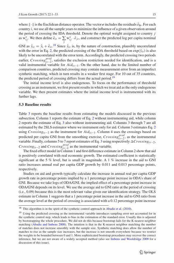
Fig. 2 Changes in Growth and Once-Lagged Changes in Aid, Two Periods after Crossing. Note Each dot is acountry. We show the relationship between changes in real per capita GDP growth two periods after crossing(�yis , where period s is two periods after crossing, y-axis), and changes in aid to GNI ratio in the previousperiod (�ln(Aid/GN I )is−1, x-axis). The slope of the fitted line is 0.08, with a standard error of 0.04

5 Foreign aid and economic growth

5.1 An illustration

The effects of aid should be most pronounced two periods after crossing, since aid volumesdropmost precipitously in the period after crossing (see earlier discussion of results in OnlineAppendix Table C). To see this, for the group of countries that cross the threshold at leasttwo periods before the end of our sample period, Fig. 2 shows the relationship between percapita real GDP growth and the once-lagged log aid to GNI ratio during the second periodafter each country crosses the threshold. We first-difference the two variables to get rid of thetime-invariant effects specific to each country. Almost all countries experienced a significantdrop in aid compared to the last period, and larger reductions in aid are associated with largerdeclines in growth.13

5.2 Econometric models

We postulate the following model in order to test the null hypothesis that aid does not affectgrowth:

gis = β1yis−1 + β2Aidis−1 + X′isβ3 + λi + τs + εis, (2)

13 Our aid and growth variables both have some measure of national income in their denominators. Bycontrolling for both income (per capita) and population andmeasuring them (and aid/GNI) in logs,weminimizethe possibility of spurious correlation due to regressing two variables with the same denominator (Kronmal1993).

123

12 J Econ Growth (2017) 22:1–33

where s denotes non-overlapping 3-year periods. Period s includes years t, t − 1, t − 2. ydenotes log real per capita GDP. gis, constructed as (yit − yit−3) /3, is the average logdifference of real GDP per capita of country i in period s. yis−1 is measured as the log realper capita GDP in the second year of the previous period (i.e., yit−4).14 We expect β1, whichcaptures conditional convergence, to be negative. Aidis−1 is the log of average aid receivedby country i as a share of GNI in the previous period.15 We use the one-period lag of aidinstead of contemporaneous aid to allow time for aid to take effect (Clemens et al. 2012).Xis is a column vector of time-varying variables, including log population, assumed to bestrictly exogenous. In the literature, population is almost always on the right hand side of aidallocation regressions (smaller countries receive more aid per capita), and it is commonlyon the right hand side in growth regressions (usually with scale effects in mind) as well.While here we show only a parsimonious model of time-varying variables, we show laterthat our results remain robust to controlling for other time-varying growth determinants. β3

is a column vector. λi is the country i fixed effect. τs−1 is the period s fixed effect.We use three alternative empirical methods in this subsection to estimate Eq. 2. Each

method requires particular assumptions.We thus report baseline results and a series of robust-ness tests using each of the three methods.

The standard way to estimate Eq. 2 is to eliminate the unobservable country-specificeffects, λi , by including a set of country dummy variables in themodel, which is equivalent todemeaningEq. 2 and estimating the transformed equation byOLS. This estimator, however, ispotentially inconsistent due to aid being also affected bygrowth,measurement error, and time-varying unobservable variables. We therefore instrument aid in period s − 1 (i.e., Aidis−1)

with a dummy variable indicating whether the country has crossed the IDA threshold by theend of period s − 2, that is, Crossingi,s−2.

Our instrumental variable is based on per capita (nominal) GNI crossing the IDA thresholdtwo periods earlier. Per capita (nominal) GNI level in period s − 2 is correlated with theidiosyncratic shock to (real) economic growth of that period, εis−2. Thus, estimating Eq. 2by means of the fixed effects estimator, which first de-means the equation, mechanicallyintroduces a correlation between the instrumental variable and the demeaned error term, ε.However, if εis is not serially correlated, the correlation between ε and εis−2 will be small ifthe time dimension of the panel is large. Our sample has 8 periods, which is not consideredshort in the literature. We also show below that we do not reject the null hypothesis of noserial correlation of the error terms in Eq. 2.16

14 Notice that, by construction, yis−1 is notmechanically correlatedwith the dependent variable. Some studiesin the literature use per capita real GDP in purchasing power parity terms to measure income level and tocalculate growth (e.g., Boone 1996). Real per capita GDP based on current exchange rates (in constant dollarterms, and using the Atlas method) and real per capita GDP in PPP terms are highly correlated (at over .95)across countries in our sample. Growth rates constructed from the two versions are essentially the same. Weuse per capita GDP based on current exchange rates (in constant dollars) because there are fewer missingobservations in the WDI database than for the PPP measure. Using instead the PPP measure we obtain almostidentical results for our basic specifications in Table 3.15 For further justification of why we use the log form, see Appendix B. In addition, the results are essentiallyunchanged when Aidis−1 is measured as the ODA share of GDP.16 When the panel is long, ε is less correlated with the error term from a particular period, and the bias willbe small. To get a sense of the potential bias in the 2SLS fixed effect model due to the mechanical correlationbetween the instrument and the demeaned error term, we conduct a Monte Carlo simulation. We assume theerror term is i.i.d. We use the predicted values from the OLS FE model and add an i.i.d. error to simulate

the outcome variable (gsimis ). We reconstruct our instrument as Crossingsimis−2 = 1{yis−3 + gsimis ≥ ys−2

},

where ys is the IDA threshold in the second year of period s. In the FE model, the instrument is thus mechan-ically correlated with the demeaned error term. We then estimate the 2SLS FE model using Crossingsimis−2 as

123

J Econ Growth (2017) 22:1–33 13

Table3

Baselineresults

Mainspecification

(1)

(2)

(3)

(4)

(5)

(6)

(7)

OLS

OLS

2SLS

2SLS

2SLS

2SLS

2SLS

Aid

is−1

0.01

050.01

330.02

810.03

520.04

750.04

850.05

52

(0.004

55)**

(0.006

15)**

(0.010

0)**

*(0.014

7)**

(0.023

9)**

(0.017

7)**

*(0.019

0)**

*

[0.004

][0.006

][0.010

][0.014

][0.023

][0.018

][0.019

]

y is−

1−0

.067

5−0

.161

−0.037

1−0

.024

9−0

.097

6−0

.095

7−0

.083

5

(0.024

6)**

*(0.023

1)**

*(0.025

6)(0.032

2)(0.051

6)*

(0.038

7)**

(0.041

5)**

[0.022

][0.022

][0.026

][0.033

][0.051

][0.039

][0.043

]

Period

FEX

XX

XX

XX

Cou

ntry

FEX

XX

Firstd

ifferenced

XX

XX

IVX

XX

XX

IVfrom

predictedincome

XX

IVfirstdifferenced

X

N24

721

224

724

721

221

221

2

Num

berof

coun

tries

3535

3535

3535

35

Firststage

Fstatistic

(K-P

Wald)

16.50

7.38

519

.52

16.16

24.06

95%

A-R

CI

[.011

8,.062

7][.013

6,0.12

47]

[−0.00

83,0.103

4][0.021

2,0.11

66]

[0.025

8,0.12

07]

AR(2)pvalue

0.72

90.83

00.82

4

Eachobservationisacountry-period.T

hedependentvariableistheperiod

averagerealpercapitaGDPgrow

thrate.S

tandarderrorsclusteredatthecoun

trylevelare

repo

rted

inparentheses,

∗ p<

0.10

,∗∗p

<0.05

,∗∗∗ p

<0.01.W

ildclusterbootstrapped

standard

errorsarereported

inbrackets.S

eetext

formoredetails

123

14 J Econ Growth (2017) 22:1–33

Although the fixed effect model could be biased, it is a starting point in our analysisand provides a useful benchmark result. Throughout the paper, we use two other methodsto circumvent this problem. The first approach is to first-difference Eq. 2 and estimate thefollowing equation:

�gis = β1�yis−1 + β2�Aidis−1 + �Xis · β3 + �τs + �εis, (3)

In using �Crossingis−2 to instrument �Aidis−1, our identification strategy exploits onlythe sharp variability in aid at the period after crossing the IDA threshold. Under treatmentheterogeneity, both in terms of the effect of threshold-crossing on aid and of the latter on eco-nomic growth, this strategywill identify a particular local average causal effect. Alternatively,we can also use just Crossingis−2 to instrument for �Aidis−1.

The validity of the exclusion restriction in this case requires the error terms εis to be seriallyuncorrelated, i.e., the instrumental variable will be invalid if the unobservable idiosyncraticerror term in the growth equation is serially correlated. Below we investigate the validity ofthis assumption.

In the first differenced model, even if the error terms were i.i.d., the transformed errorterms will not be, and will exhibit first-order serial correlation. Standard GMM inferencewhen using optimal weights takes into account this feature while 2SLS does not. Thus,through the rest of the paper, as in the previous section, we rely on two alternative methodsto conduct statistical inference. We report in parentheses robust standard errors clustered atthe country level, which allow for within-country correlation. We also report in brackets thestandard errors from the wild clustered bootstrap procedure. Both methods render similarstatistical conclusions for our main parameters.

The second alternative to the 2SLS-FE model relies on a smoothing method of the latentprocess that determines our instrumental variable. Intuitively, we form a “synthetic control”for each crossing country using countries that are not in our sample. The synthetic control isconstructed in such away that the distance between income trajectories of the crossing countryand its synthetic control is minimized. We then use the income trajectories of the syntheticcontrol to predict the year of crossing, which is a function of shocks to other countries. Underthe assumption that shocks across countries are not correlated (after controlling for all thecovariates in Eq. 2), the predicted crossing is not correlated with εis−2.

Specifically, we proceed to construct our synthetic control as follows. We include a panelof 130 other developing countries thatwere officialDACaid recipient countries between 1987and 2010, together with the 35 countries in our original sample.17 We demean all the seriesin our extended panel (of 165 countries) by projecting the annual log of nominal per capitaGNI onto a set of country fixed effects, denoted yi. We then take the residuals, eit . For each ofthe 35 countries in our working sample, we construct a set of weights w j ∈ {w1,w2, ...,wJ}bounded between 0 and 1 for the 130 recipient countries such that the following distancefunction is minimized:

Di = ‖ei −∑

j

w j · e j‖, (4)

(Footnote 16 continued)the instrumental variable for aid and gauge the magnitude of the bias. We repeat this procedure 1,000 times,take the mean of 2SLS FE estimate and compare it with the OLS FE estimate (the true parameter). We estimatea negligible bias of less than 2 % of the true parameter value.17 Since both our sample and the extended dataset are unbalanced panels, for each of the 35 countries in oursample we use only a balanced panel of available donors.

123

J Econ Growth (2017) 22:1–33 15

where ‖·‖ is the Euclidean distance operator. The vector e includes the residuals eht. For eachcountry i , we use all the sample years to minimize the influence of a given observation aroundthe period of crossing the IDA threshold. Denote the optimal weight assigned to country jas w∗

i j . We then define ei t = ∑

jw∗i j · e j t , and construct the predicted log per capita nominal

GNI as yi t = yi + ei t .18 Since yi t is, by the nature of construction, plausibly uncorrelatedwith the error in Eq. 2, the predicted crossing of the IDA threshold based on exp(yi t ) is alsolikely to be uncorrelated with the error term. Accordingly, the predicted crossing two periodsearlier, Crossingpred

is−2 , satisfies the exclusion restriction needed for identification, and is avalid instrumental variable for Aidis−1. On the other hand, due to the limited number ofcomparison countries, predicted crossing may contain measurement error from an imperfectsynthetic matching, which in turn results in a weaker first stage. For 10 out of 35 countries,the predicted period of crossing differs from the actual period.19

The initial income level is also endogenous. To focus on the performance of thresholdcrossing as an instrument, we first present results inwhichwe treat aid as the only endogenousvariable. We then present estimates where the initial income level is instrumented with itsfurther lags.

5.3 Baseline results

Table 3 reports the baseline results from estimating the models discussed in the previoussubsection. Column 1 reports the estimate of Eq. 2 without instrumenting aid, while column2 reports the estimate of Eq. 3 also without instrumenting aid. Columns 3 through 7 are allestimated by the 2SLS estimator where we instrument only for aid. Column 3 estimates Eq. 2using Crossingis−2 as the instrument for Aidis−1. Column 4 uses the crossings based onpredicted per capita GNI from the smoothing exercise, Crossingpred

is−2 , as the instrumentalvariable. Finally, columns 5 to 7 report estimates of Eq. 3 using respectively�Crossingis−2,Crossingis−2 and Crossing

predis−2 as the instrumental variable.

The fixed effect model in Column 1 and first difference estimate in Column 2 show that aidis positively correlated with real economic growth. The estimated coefficient is statisticallysignificant at the 5 % level, but is small in magnitude. A 1 % increase in the aid to GNIratio increases annual real per capita GDP growth by 0.011 and 0.013 percentage points,respectively.

Studies on aid and growth typically calculate the increase in annual real per capita GDPgrowth rate in percentage points implied by a 1 percentage point increase in ODA’s share ofGNI. Because we take logs of ODA/GNI, the implied effect of a percentage point increase inODA/GNI depends on its level. We use the average aid to GNI ratio at the period of crossing(i.e., 0.09) because this is the most relevant value given our identification strategy. The OLSestimate in Column 1 suggests that a 1 percentage point increase in the aid to GNI ratio fromthe average level at the period of crossing is associated with a 0.12 percentage point increase

18 This algorithm is in the spirit of the synthetic control approach in Abadie et al. (2010).19 Using the predicted crossing as the instrumental variable introduces sampling error not accounted for inthe synthetic control step, which leads to bias in the estimation of the standard error. Usually this is adjustedby bootstrapping the whole procedure. We did not do this because bootstrap fails for the K-nearest neighbormatching (Abadie and Imbens 2008). The intuition is that in the K-nearest neighbor matching the numberof matches does not increase smoothly with the sample size. Synthetic matching does allow the number ofmatches to rise as the sample size increases, but the increase is not smooth everywhere because we restrictthe weights to be bounded between 0 and 1. More sophisticated bootstrap procedures may recover the correctinference, but we are not aware of a widely accepted method (also see Imbens and Wooldridge 2009 for adiscussion of this issue).

123

16 J Econ Growth (2017) 22:1–33

in real per capita GDP growth. The result in Column 2 implies that a 1 percentage pointincrease in the aid to GNI ratio from the same level is associated with a 0.14 percentage pointincrease in growth, consistent with the magnitudes obtained by Clemens et al. (2012). Theyaddress endogeneity of aid simply by lagging it one period in a fixed-effects regression, asin our Column 1, and find that a one percentage point increase in aid/GDP from the samplemean increases annual real per capita GDP growth by 0.1 to 0.2 percentage points in thenext (4-year) period. Werker et al. (2009) estimate a slightly larger effect of 0.22 percentagepoints instrumenting aid with the interaction between oil and a dummy indicating a Muslimcountry.

Columns 3 through 7 are estimated using the 2SLS method. The point estimates of theaid coefficient are more than twice as large as those estimated by OLS. In column 3 weuse Crossingis−2 as the instrument for Aidis−1. Now a 1 % increase in the aid to GNIratio raises growth by 0.028 percentage points. The first stage is strong, with an F-statisticof about 16.20 Growth is negatively correlated with lagged income, supporting conditionalconvergence.21 In column 4 we use the predicted crossings based on the smoothed per capitaGNI trajectory, Crossingpred

is−2 , as the instrument. The estimated coefficient associated withAidis−1 increases slightly to 0.035, and is statistically significant at the 5 % level. The firststage is weaker with an F-statistic of 7.4. We also report the Anderson-Rubin (AR) 95 %confidence intervals for the coefficient associated with aid. These confidence intervals arerobust to potential weak instruments (Finlay and Magnusson 2009). Almost all of theseconfidence intervals lie entirely to the right of zero. Note the similarity of the point estimatesof the effect of aid on growth in columns 3 and 4.

Columns 5 through 7 estimate the first differenced model in Eq. 3. The coefficients areall larger than those in Column 3 and Column 4. Column 5 uses �Crossingis−2 as theinstrumental variable for �Aidis−1. In this specification, we estimate the coefficient of aidusing only the variability from the one period after crossing. The aid coefficient is 0.047.Column 6 uses Crossingis−2 as the instrumental variable for �Aidis−1. The first stageand the estimated coefficients are essentially unchanged from those in column 5. Column 7uses the predicted crossing, Crossingpred

is−2 , as the instrument. The first stage is strong, withan F-statistic of 24. The aid coefficient is 0.055, statistically significant at the 1 % level.Overall, our instrumental variable estimates are robust and consistently larger than the OLSestimates.22

As discussed earlier, for the first differenced model, our instrumental variable will beinvalid if the unobservable idiosyncratic error term in the growth Eq. 2 is serially correlated.We test for the presence of serial auto-correlation in the error terms inEq. 2 followingArellanoand Bond (1991). The Arellano–Bond test for serial correlation tests the nth order of serialcorrelation of the first differenced error to infer the (n − 1)th order of serial correlation ofthe error terms in the original equation (see also Roodman 2009a). We report the p values of

20 A large F-statistic suggests a strong first stage, alleviating the concern of potential severe bias due to weakinstruments. For linear models with only one endogenous variable, Stock and Yogo (2005) suggest a rule-of-thumb cutoff for a first stage F-Statistic of about 10. This heuristic criterion does not apply straightforwardlyto more complicated specifications presented below.21 Column 3 of Online Appendix Table C presents the estimates of the same specification as in Column 3of Table 3, but using Crossingis−1,Crossingis−2, and Crossingis−3 as instrumental variables. The pointestimate of the effect of aid on growth remains very similar, but the first stage is weaker than in our baselinespecification.22 If we re-estimate the model in column 3 of Table 3 while including quadratic and cubic terms of yis−1,the results remain similar (as shown in Online Appendix Table H).

123

J Econ Growth (2017) 22:1–33 17

the Arellano–Bond test for AR(2) after estimations in Columns 5, 6, and 7. None of the testsrejects the null hypothesis of no serial correlation in the errors in Eq. 2.

So far we have treated Aidis−1 as the only endogenous variable. However, the initialincome level, yis−1, could also be endogenous. In particular, when we first difference themodel,�yis−1 ismechanically correlatedwith the first-differenced error term. Table 4 reportsestimates where we also instrument yis−1 following the standard procedures in the literature.We therefore test for whether the model is under-identified. The p values of the Kleibergen-Paap rank Lagrange Multiplier (LM) test uniformly reject the null hypothesis that the modelis under-identified. Columns 1 and 2 re-estimate the models in columns 3 and 4 of Table 3,respectively, but also instrumenting yis−1 (i.e., yit−4) with yit−5. Column 3 re-estimates themodel in column 6 of Table 3 and uses yit−8 to instrument for �yis−1 (i.e., yit−4 − yit−7).The aid coefficient remains similar. Columns 4 and 5 are estimated by the difference GMMestimator, which is widely used in this literature. Given the potential problems with manyinstruments in finite samples, we use a parsimonious set of instruments (Roodman 2007,2009a, b; Bazzi and Clemens 2013; Bun and Windmeijer 2010), namely yit−8, yit−9, andyit−10. We use Crossingi,s−2 as an instrument in Column 4 and Crossingpred

i,s−2 in Column5. With more instruments than endogenous variables, we can test the validity of the over-identifying restrictions, and both the Sargan andHansen tests do not reject the null hypothesisof their validity. In order to compare with other columns in terms of instrument strength, wereport the first-stage F-statistics based on estimating the corresponding 2SLS models withthe same specification as in the GMM model.

The failures to reject the validity of the over-identification restrictions or the null of noserial correlation in the error term in Eq. 2 suggest that the error terms in the growth equationare serially uncorrelated. Besides these two pieces of evidence, we also provide a thirdpiece of evidence. If the error terms were serially correlated, including lagged values of thedependent variable will alter the estimates of the aid coefficient. Including lagged values ofthe dependent variable on the right-hand-side also controls for any positive shocks to growthbefore crossing which are eventually reversed. We thus re-estimate the model in Column 3of Table 3 but include the once-lagged value of the dependent variable as a control variable(Column 6 of Table 4), or its twice-lagged value (Column 7), and then both the once- andtwice-lagged values (Column 8). Columns 9, 10, and 11 of Table 4 repeat Columns 6, 7, and8 but using Crossingpred

i,s−2 to instrument aid. Estimates of the effect of aid remain sizable

and similar to those in Table 3.23

The estimated effects of aid on growth in Columns 1 to 5 in Table 4 are all very similar toeach other. Taking the point estimate in Column 2 we observe that a 1 % increase in the aid toGNI ratio increases real per capita GDP growth by 0.031 percentage points. A 1 percentagepoint increase in the aid to GNI ratio from its average value at the period of crossing (0.09)thus raises the growth rate by 0.35 percentage points (i.e.,.031*[.01/.09]*100).24

23 In column 3 of Table 4, we find that the clustered standard errors and the robust standard errors are verysimilar (results not shown). The similarity between the two sets of standard errors is consistent with theevidence of lack of serial correlation of the error term in Eq. 2.24 We report the robust first-stage F statistic for the overall strength of the first stage (Kleibergen-Paap rankWald F statistic) for specifications in Table 4. With multiple endogenous variables, the first stage F statistic isless informative than the case of one instrument. We thus construct 95%Anderson-Rubin confidence intervalsfor the coefficients associated with endogenous variables that are robust to weak instruments (Finlay andMagnusson 2009). With two endogenous variables, the confidence interval of a particular coefficient dependson the value of the coefficient associated with the other endogenous variable. Thus the confidence intervalfor both endogenous variables will be a two-dimensional figure. We report these graphs for specifications inTable 4 in Online Appendix Figure A. Overall, the 95 % confidence intervals for the aid coefficient lie entirely

123

18 J Econ Growth (2017) 22:1–33

Table4

Alternativespecificatio

ns

Mainspecification

(1)

(2)

(3)

(4)

(5)

(6)

(7)

(8)

(9)

(10)

(11)

2SLS

2SLS

2SLS

GMM

GMM

2SLS

2SLS

2SLS

2SLS

2SLS

2SLS

Aid

is−1

0.02

580.03

120.04

270.02

980.03

080.01

980.02

290.02

050.03

310.03

590.03

77

(0.009

66)***

(0.013

8)**

(0.018

2)**

(0.012

2)**

(0.013

3)**

(0.009

84)**(0.010

1)**

(0.009

09)**(0.014

9)**

(0.015

2)**

(0.015

5)**

[0.010

][0.013

][0.018

][0.010

][0.010

][0.010

][0.014

][0.015

][0.015

]

y is−

1−0

.052

5−0

.043

1−0

.137

−0.128

−0.136

−0.054

0−0

.054

3−0

.051

8−0

.032

6−0

.033

4−0

.024

5

(0.022

6)**

(0.029

0)(0.067

9)**

(0.055

4)**

(0.052

9)**

*(0.018

4)**

*(0.021

7)**

(0.020

1)**

(0.028

2)(0.028

1)(0.026

1)

[0.023

][0.029

][0.069

][0.019

][0.022

][0.022

][0.022

][0.028

][0.026

]

Period

FEX

XX

XX

XX

XX

XX

Cou

ntry

FEX

XX

XX

XX

X

Firstd

ifferenced

XX

X

IVfory is−

1X

XX

XX

XX

XX

XX

Predictedcrossing

XX

XX

X

lagged

dependentv

ariables

12

1,2

12

1,2

N24

724

721

221

221

224

522

922

924

522

922

9

Num

berof

coun

tries

3535

3535

3535

3535

3535

35

Firststage

Fstatistic

(K-P

Wald)

8.09

83.60

111

.46

4.45

36.16

45.95

16.52

06.44

83.26

34.08

34.10

3

Under-id(K

-Prank

LM)(p

value)

0.00

10.01

20.00

00.00

40.00

10.00

20.00

20.00

20.01

50.01

00.00

9

Num

berof

IVs

1212

Hansentestforover-id(p

value)

0.33

00.17

4

Sargan

testforover-id(p

value)

0.27

50.10

6

AR(2)pvalue

0.95

00.84

9

Eachob

servationisacoun

try-period

.The

depend

entv

ariableistheperiod

averagerealpercapitaGDPgrow

thrate.Instrum

entalv

ariablefory is−

1isy it−

5allcolum

nsexcept

forColum

ns3,

4,5.

y is−

1isinstrumentedby

y it−

8in

Colum

n3,

andisinstrumentedby

y it−

8,y it−

9,and

y it−

10in

Colum

ns4and5.

Standard

errorsclusteredatthecoun

try

levelare

reported

inparentheses,

∗ p<

0.10

,∗∗p

<0.05

,∗∗∗ p

<0.01.W

ildclusterbootstrapped

standard

errorsarein

brackets.S

eetext

formoredetails

123

J Econ Growth (2017) 22:1–33 19

5.4 Measurement error in aid

Aid/GNI is likely to be measured with error, and this possibility is consistent with the obser-vation that the 2SLS estimates are larger than the OLS estimates. There are various reasonswhy aid is measured with error. Not all donors report their aid to the DAC in all years. Forexample, aid from the former Soviet Union and from China in the Mao era to other com-munist countries was not reported to the DAC. Aid from China and other emerging donorshas significantly increased in recent years but is mostly not reported. The official definitionof aid counts $1 in grants the same as $1 in concessionary loans (for any loan with a grantelement of at least 25 %). Additionally, but better understood, the denominator, GNI, is alsomeasured with sizeable error for many less developed countries (Jerven 2013). With classicmeasurement error, the OLS estimate of the effect of aid is biased towards zero. Demeaningor first differencing the model likely exacerbates the bias.

The natural experiment we exploit in this paper provides a unique opportunity to gauge themagnitude of the attenuation bias in the OLS estimation due to measurement error. We haveshown that the amount of aid a country receives declines substantially following its crossingof the IDA threshold. Assuming that the measurement error is i.i.d., it would contributemuch less to the total variation in �Aidis in periods closer to threshold crossings. Thus theOLS estimates of Eq. 4 using only periods in the neighborhood of the crossings are likelyto provide more accurate estimates of aid’s effect on growth than the one exploiting all ofthe variability in aid from all periods. To test this, we re-estimate Eq. 4 by OLS and 2SLS(usingCrossingi,s−2 to instrument aid), successively narrowing the window of periods usedin the analysis around the crossing point of each country.25 We expect the OLS estimate ofthe aid effect on growth to increase as we narrow the window of estimation. Naturally, thecoefficient in the 2SLS estimate of the first-differenced model should remain stable as thewindow narrows, because it uses only a single period for identification. We find exactly thatpattern in Table 5, Panel B.

Panel A of Table 5 reports the OLS estimates. As we narrow the window, the estimatedcoefficient associatedwith foreign aidmonotonically and gradually increases. The coefficientin Column 6 (withmaximal two periods around the crossing) is 0.0201,more than 50% largerthan that in Column 1 (with maximal 7 periods around the crossing). A generalized Hausmantest of the null hypothesis that the coefficient associated with Aidis−1 is the same in Column1 and in Column 6 is rejected with a p value of 0.07. These findings are consistent with theexistence of significant measurement errors in the ratio of aid to GNI.26

5.5 Bunching

Our identification strategy hinges on the large decline in the amount of aid received followingthe crossingof a pre-determined threshold. If countriesmanipulate their incomedata to remainbelow the threshold, then threshold crossing may not be a valid instrument for aid.

to the right of zero (except for Column 4 in which we obtain significance only at the 10 % level, and we showthe plot for the 90 % confidence interval).25 We rely on first differenced models in this exercise because changing the number of periods also affectsthe estimation of the country fixed effects, and we want to hold everything constant except for the signal tonoise ratio in aid.26 Needless to say, as discussed extensively through the paper, this is not the only source of potential endo-geneity in aid. Furthermore, we note that the discussion above is based on the assumption of a homogeneouseffect of log aid. Relaxing this assumption, the results found in Table 5 would also be consistent with thepresence of heterogeneous effects where aid has the largest effect around the IDA threshold (instead of whencountries were poorer).

123

20 J Econ Growth (2017) 22:1–33

Table5

Narrowingperiod

s

(1)

(2)

(3)

(4)

(5)

(6)

76

54

32

PanelA

:OLS-firstdifferenced#of

maxim

alperiod

sarou

ndthecrossing

s

Aid

is−1

0.01

330.01

330.01

370.01

420.01

540.02

01

(0.006

15)**

(0.006

15)**

(0.006

40)**

(0.006

31)**

(0.008

14)*

(0.009

46)**

[0.006

][0.006

][0.006

][0.006

][0.008

][0.009

]

y is−

1−0

.161

−0.161

−0.162

−0.163

−0.161

−0.157

(0.023

1)**

*(0.023

2)**

*(0.023

2)**

*(0.023

5)**

*(0.025

6)**

*(0.029

8)**

*

[0.022

][0.022

][0.022

][0.022

][0.024

][0.028

]

Period

FEX

XX

XX

X

N21

221

120

318

816

513

3

Num

berof

coun

tries

3535

3535

3535

TestforAid

is−1

((6)-(1),pvalue)

0.06

9

123

J Econ Growth (2017) 22:1–33 21

Table5

continued

(1)

(2)

(3)

(4)

(5)

(6)

76

54

32

PanelB

:2SL

S-firstdifferenced#of

maxim

alperiod

sarou

ndthecrossing

s

Aid

is−1

0.04

850.04

810.04

600.04

420.04

270.05

27

(0.017

7)**

*(0.017

7)**

*(0.018

1)**

(0.015

7)**

*(0.019

2)**

(0.022

2)**

Wildclusterbootstrap-tp

value

[0.018

][0.018

][0.018

][0.016

][0.019

][0.022

]

y is−

1−0

.095

7−0

.096

9−0

.103

−0.107

−0.113

−0.104

(0.038

7)**

(0.038

9)**

(0.039

7)**

*(0.036

9)**

*(0.044

1)**

(0.048

8)**

Wildclusterbootstrap-tp

value

[0.039

][0.040

][0.041

][0.038

][0.045

][0.048

]

Period

FEX

XX

XX

X

N21

221

120

318

816

513

3

Num

berof

coun

tries

3535

3535

3535

Firststage

Fstatistic

(K-P

Wald)

16.159

16.353

15.741

19.946

16.577

19.971

TestforAid

is−1

((6)-(1),pvalue)

1.00

0

Eachobservationisacountry-period.T

hedependentv

ariableistheperiod

averagerealpercapitaGDPgrow

thrate.T

hegrow

thequatio

nisfirstdifferencedbefore

estim

ation.

IVin

thefirstdifferencedequatio

nisCro

ssing is−

2.S

tandarderrorsclusteredatthecountrylevelare

reported

inparentheses,

∗ p<

0.10

,∗∗p

<0.05

,∗∗∗ p

<0.01

.Stand

ard

errorsfrom

thewild

clusterbo

otstrapprocedurearerepo

rted

inbrackets.T

hepvalueof

theHausm

antestwith

thenullhypothesisthatthecoefficientsassociated

with

Aid

is−1

inColum

n1andColum

n6arethesameisrepo

rted

ineach

panel

123

22 J Econ Growth (2017) 22:1–33

Endogenous manipulation of the income level is unlikely to be prevalent for three rea-sons. First, the GNI estimates used by the World Bank are by no means entirely within agovernment’s control. The national accounts data produced by national statistical agenciesare merely one of several inputs into theWorld Bank’s income estimates (Jerven 2013). Gov-ernments cannot perfectly predict (1) the adjustments to those national accounts data oftenmade by World Bank staff, (2) the exchange rates used, or (3) the population estimates usedin constructing GNI per capita. Second, crossing also depends on the current IDA thresh-old, and its annual adjustments for global inflation rates cannot be predicted perfectly either.Finally, income level with respect to the threshold is not the only criterion for IDA eligibility;e.g. countries that cross the threshold from below can remain eligible if they are judged tobe non-creditworthy for non-concessionary lending.

Even if governments manipulated GNI to delay their graduation from IDA, the resultingbias would work against our main finding. Note that GNI per capita and its growth wouldbe understated prior to crossing the threshold, when aid is relatively high. After crossing,there would be little reason to continue understating GNI per capita, and correcting it wouldoverstate growth for at least one period after crossing, when aid is relatively low.

Nevertheless, we tested for evidence of data manipulation. Figure 3a is a histogram thatshows the distance between a country’s current GNI per capita and the contemporaneous IDAthreshold. All countries that were ever eligible for IDA between 1987 and 2010 are included,and each GNI per capita value in each country-year is treated as a separate observation. Wegroup country-year observations in 100-dollar bins according to the distance between theincome level and the contemporaneous IDA threshold. If many governments understate GNIto stay below the IDA threshold, we should observe significant “bunching” of observationsjust below the threshold, relative to the number of observations just above it. Specifically,we should observe the bin just to the left of the threshold to be abnormally high relative tothe neighboring bins. If there is no bunching, the numbers of observations in each bin shouldcross the threshold of zero smoothly. As shown in Fig. 3a, there is no visual evidence thatcountries bunch right below the IDA threshold. A formal test confirms this result. Usinga density test proposed by McCrary (2008), we find no significant evidence of bunching.Figure 3b is a density graph that shows the fitted kernel density functions at both sides ofthe threshold. The density crosses the IDA threshold smoothly, and the minor difference isby no means statistically significant.

5.6 Further robustness checks

We next present various additional robustness tests, for which we report two sets of results.These tests all use either Crossingi,s−2 or Crossingpred

i,s−2 as the instrument for aid. Theyare all based on our preferred specification in Column 3 of Table 3 (or Column 4 of Table 3when Crossingpred

i,s−2 is used as the instrument). As we shall see, these robustness checks

yield results that are largely consistent with our main findings.27

Throughout the study, we control for period fixed effects, log of initial income, and logof population. Period fixed effects take account of any time-specific shocks that affect allcountries. Initial income and population are among the key time-varying factors that affecteconomic growth.We also control for country fixed effects that account for any time-invariantdeterminants of the level of growth rate, including most slow-moving factors (over our rela-tively short 1987–2010 period) such as the quality of governance.Herewe further testwhetherother time-varying factors could be confounding the effect of aid on economic growth, by

27 Results are also robust to other specifications in Table 3.

123

J Econ Growth (2017) 22:1–33 23

0.0

005

.001

.001

5

dens

ity

−1000 −500 0 500 1000

income−IDA threshold

Density of (income−IDA threshold)

0.0

005

.001

.001

5

−2000 −1000 0 1000 2000

A

B

Fig. 3 a Histogram of income. bMcCrary test of bunching. Note There are 1,920 country-year observationsfrom 112 countries that were ever on the DAC list between 1987 and 2010. For each country-year observation,we calculate the distance of the current per capita GNI (yit ) from the current IDA threshold (yt ). We restrictthe distance (yit − yt ) between −1000 and 1000. Graph A is a histogram of country-year observations against(yit − yt ), grouped in 100-dollar bins. Graph B shows the McCrary density test. The discontinuity estimate(log difference in height from left to right) is −0.0476, with a standard error of 0.1776

adding to the baseline regression a host of economic and political variables, including theprimary school enrollment rate, the Freedom House index of civil liberty and political rights,the World Bank’s Country Policy and Institutional Assessment (CPIA) ratings, total tradeas a percentage of GDP, broad money as a percentage of GDP, inflation as measured bychanges in the GDP deflator, dummies for whether the country is experiencing a bankingcrisis, currency crisis, or debt crisis (central government debt/GNI is available for fewer thanhalf of the countries in our sample), and a survey-based measure of country creditworthinessfrom Institutional Investor. Due to missing values, we add these variables in separate groupsto maintain a reasonable sample size for each regression. Table 6 shows the results of theseexercises. Few of the additional regressors have a statistically significant effect on growthin either set of estimations for our relatively small sample of countries. The aid coefficients

123

24 J Econ Growth (2017) 22:1–33

Table6

Addingcovariates

(1)

(2)

(3)

(4)

(5)

(6)

(7)

(8)

(9)

(10)

(11)

(12)

IVisCro

ssing is−

2IV

isCro

ssingpred

is−2

Baseline

Scho

oling

Political

CPIA

Econcond

Credit

ratin

gBaseline

Scho

oling

Political

CPIA

Econcond

Credit

ratin

g

Aid

is−1

0.02

810.03

070.02

870.03

360.03

080.03

03**

0.03

520.03

930.03

680.03

830.04

560.03

31**

*

(0.010

)***

(0.011

)***

(0.010

2)**

*(0.010

5)**

*(0.011

)***

(0.012

5)(0.014

7)**

(0.015

2)**

*(0.015

8)**

(0.014

8)**

*(0.020

5)**

(0.013

4)

y is−

1−0

.037

1−0

.040

2−0

.036

1−0

.023

2−0

.011

9−0

.074

0**

−0.024

9−0

.024

5−0

.022

2−0

.015

30.01

01−0

.033

0

(0.025

6)(0.027

3)(0.026

2)(0.024

1)(0.026

9)(0.030

3)(0.032

2)(0.033

2)(0.034

3)(0.032

1)(0.037

7)(0.037

8)

Log

popu

latio

n−0

.008

6−0

.014

9−0

.011

40.04

230.01

33−0

.082

40.01

610.02

030.01

490.05

840.05

710.00

67

(0.073

8)(0.075

3)(0.075

4)(0.076

7)(0.055

6)(0.085

7)(0.085

9)(0.086

9)(0.087

9)(0.090

3)(0.085

8)(0.103

0)

Prim

aryscho

olenrolm

entrate

−0.000

3−0

.000

3

(0.000

4)(0.000

5)

Freedo

mho

usecivilliberty

0.00

23−0

.003

60.00

380.00

21−0

.004

50.00

21

(0.007

3)(0.006

2)(0.006

3)(0.007

8)(0.006

1)(0.007

1)

Freedo

mho

usepo

liticalrigh

ts0.00

130.00

04−0

.001

80.00

260.00

11−0

.000

1

(0.004

2)(0.004

0)(0.003

9)(0.004

4)(0.003

9)(0.004

1)

World

BankCPIA-Z

score

0.01

51*

0.01

56*

(0.008

2)(0.008

2)

Totaltrade

as%

ofGDP

0.00

070.00

06

(0.000

5)(0.000

5)

Broad

mon

ey−0

. 000

3−0

.000

2

(0.000

6)(0.000

6)

Inflatio

n(G

DPdeflator)

−0.000

0**

−0.000

0**

(0.000

0)(0.000

0)

123

J Econ Growth (2017) 22:1–33 25

Table6

continued

(1)

(2)

(3)

(4)

(5)

(6)

(7)

(8)

(9)

(10)

(11)

(12)

IVisCro

ssing is−

2IV

isCro

ssingpred

is−2

baselin

escho

oling

political

CPIA

econ

cond

creditratin

gbaselin

escho

oling

political

CPIA

econ

cond

creditratin

g

Bankcrisisdu

ring

theperiod

0.00

560.00

45

(0.011

7)(0.013

4)

Currencycrisisdu

ring

theperiod

−0.002

30.00

23

(0.009

7)(0.011

0)

Debtcrisisdu

ring

theperiod

−0.009

5−0

.008

0

(0.016

2)(0.015

4)

Creditrating

0.00

08*

0.00

05

(0.000

4)(0.000

4)

Period

FEX

XX

XX

XX

XX

XX

X

Cou

ntry

FEX

XX

XX

XX

XX

XX

X

N24

722

424

723

822

519

524

722

424

723

822

514

7

Num

berof

coun

tries

3534

3535

3334

3534

3535

3325

Firststage

Fstatistic

(K-P

Wald)

16.495

14.469

16.389

16.459

13.647

8.25

87.38

57.90

96.59

07.73

25.25

96.48

2

Eachobservationisacountry-period.T

hedependentv

ariableistheperiod

averagerealpercapitaGDPgrow

thrate.A

llcolumns

areestim

ated

using2S

LS.

Colum

ns1throug

h6useactual

crossing

sas

instrument.Colum

ns7throug

h12

usepredictedcrossing

sas

instrument.Standard

errors

clusteredat

thecoun

trylevelarereported

inparentheses,

∗ p<

0.10

,∗∗p

<0.05

,∗∗∗p

<0.01

123

26 J Econ Growth (2017) 22:1–33

remain similar in magnitude to their counterparts in the baseline regressions; the coefficientof our key aid variable range from 0.028 to 0.046, all statistically significant at conventionallevels.

Recall that our instrument is a dummy variable that switches from 0 to 1 when a countryhas crossed the income threshold from below two periods earlier. The countries in our sampleall crossed the threshold at some point between 1987 and 2010, but for countries that crossedthe threshold in the last and the next-to-the-last periods (i.e. in periods 7 or 8) the instrumentaldummy variable is always zero. We keep these countries in the sample because they satisfyour simple rule for sample selection and they provide relevant information for estimatingthe effects of the control variables. We now check whether our results still hold when wedrop these countries. In Column 1 of Panel A in Table 7, we drop the seven countries thatcrossed the threshold in the final period of our sample (2008–2010). The point estimateincreases (to 0.041) and remains statistically significant at conventional levels. In Column2 we further drop the seven countries that crossed the threshold in the next-to-last period(2005–2007). The coefficient is slightly larger (that is, at 0.045) than that in Column 1 andremains statistically significant at the 5 % level. The first stage remains strong in each case.The first stage is weaker when we use Crossingpred

i,s−2 as the instrument in panel B, but theresults are qualitatively similar.

As shown in Table 1, a few countries crossed the IDA threshold from below more thanonce during the sample period. These countries must have crossed the threshold from aboveafter their first crossings from below, then crossed from below again. These cases might be athreat to our identification strategy. If income drops below the threshold again immediatelyafter the first crossing for any reason other than a decline in aid, the estimated effect of aidmight be confounded. In Column 3 of Panel A of Table 7, we drop countries with multiplecrossings. The estimated effect of aid (0.026) remains similar. In Column 4, we use the lastthreshold crossing (from below) instead of the first one to construct the instrumental variable.The estimated effect of aid on growth (0.024) again remains similar relative to the baselinespecification. It remains statistically significant in panel A, but in panel B the standard errorsincrease and we cannot reject the null hypothesis of no effect at conventional levels.

There are two exceptional groups of countries in the sample. First, several countries inthe sample benefit from the “small island country exception,” which permits island nationswith populations below 1.5 million to remain IDA eligible, even after surpassing the incomethreshold. Second, a few countries were never classified as IDA eligible in the 1987–2010period due to various reasons, despite having income levels below the threshold for one ormore years. We include them in the sample because the IDA income threshold potentiallyserves as a useful benchmark for donors other than IDA. In Column 5 of Table 7 we drop thethree small island countries. In Column 6, we drop the four countries that were never eligiblefor IDA throughout the sample period. The estimated effects of aid are robust to these samplechanges, with the coefficient ranging from 0.027 to 0.03.

6 Potential mechanism

Given the positive effect found in this paper, an important question is the mechanism bywhich aid boosts growth. In the short run, an important channel through which aid couldcause growth is through fostering physical investment. Irrespective of the form aid takes, itconstitutes a flow of funds to recipient countries, which, if they are financially and perhapsfiscally constrained (see Kraay 2012), would release resources in the economy that could be

123

J Econ Growth (2017) 22:1–33 27

Table7

Mod

elrobustness

checks

(1)

(2)

(3)

(4)

(5)

(6)

Excl.lastxing

Excl.last2xing

Multip

lecrossings

Lastcrossings

Smallislands

Non

IDA

PanelA

:IVisCro

ssing is−

2

Aid

is−1

0.04

130.04

510.02

570.02

410.02

730.02

99

(0.017

2)**

(0.018

6)**

(0.009

91)***

(0.011

2)**

(0.009

3)**

*(0.012

0)**

[0.018

][0.026

][0.010

][0.011

][0.010

][0.012

]

y is−

1−0

.019

4−0

.020

0−0

.071

7−0

.044

0−0

.039

6−0

.019

4

(0.033

7)(0.036

6)(0.026

3)**

*(0.032

0)(0.025

1)(0.025

9)

[0.035

][0.042

][0.026

][0.032

][0.025

][0.026

]

Period

FEX

XX

XX

X

Cou

ntry

FEX

XX

XX

X

N19

315

120

824

722

522

0

Num

berof

coun

tries

2821

3035

3231

Firststage

Fstat

8.63

520

.06

18.48

19.04

14.39

11.97

PanelB

:IVisCro

ssingpred

is−2

Aid

is−1

0.05

800.08

830.02

480.02

580.03

240.03

82

(0.029

4)**

(0.057

0)(0.013

8)*

(0.015

9)(0.012

4)**

*(0.017

2)**

[0.034

][0.124

][0.014

][0.014

][0.013

][0.017

]

123

28 J Econ Growth (2017) 22:1–33

Table7

continued

(1)

(2)

(3)

(4)

(5)

(6)

excl.lastx

ing

excl.last2

xing

multip

lecrossings

lastcrossings

smallislands

nonID

A

y is−

10.00

745

0.03

87-0.073

6−0

.041

1−0

.030

8−0

.003

46

(0.049

3)(0.086

1)(0.033

2)**

(0.040

6)(0.028

9)(0.034

5)

[0.057

][0.157

][0.034

][0.032

][0.030

][0.034

]

Period

FEX

XX

XX

X

Cou

ntry

FEX

XX

XX

X

N19

315

120

824

722

522

0

Num

berof

coun

tries

2821

3035

3231

Firststage

Fstatistic

s(K

-PWald)

3.40

11.90

56.43

88.15

87.95

85.94

6

Eachobservationisacountry-period.T

hedependentv

ariableistheperiod

averagerealpercapitaGDPgrow

thrate.S

amplerestrictions

aremarkedin

theshorth

andlein

each

column.Allcolumns

areestiamtedusing2S

LS.

PanelA

uses

actualcrossingsas

theinstrumentalvariable.PanelB

uses

predictedcrossingsas

theinstrumentalvariable.Standard

errorsclusteredatthecountrylevelare

reported

inparentheses,

∗ p<

0.10

,∗∗p

<0.05

,∗∗∗ p

<0.01.W

ildclusterbootstrapped

standard

errorsarereported

inbrackets

123

J Econ Growth (2017) 22:1–33 29

invested. Because our sample countries were all financially constrained by definition, this isa relevant scenario. Admittedly, our findings here do not rule out other mechanisms nor canthey necessarily be extrapolated to countries that are more developed and have better accessto credit markets.

We consider the expected effect of an increase of 1 percentage point in the ratio of aidto GDP if it were fully invested in physical capital. Approximating the technology at theaggregate level of the economy linearly, the rate of economic growth would increase inthe inverse of the capital-output ratio.28 Using the standard perpetual inventory method, weestimate this ratio to be approximately equal to 2 in our sample.29 Thus, one would expectthat growth could increase by as much as 0.5 percentage points if all of the aid were invested.

How much aid fosters physical investment is therefore an empirical question. To this end,in Online Appendix Table I we re-estimate the baseline specifications in Table 3, replacingeconomic growth with the period average investment to GDP ratio as the dependent vari-able. The OLS estimates in Column 1 and Column 2 of the effect of aid on investment arestatistically insignificant and have the “wrong” sign. Instrumenting aid in Columns 3 to 7,we find that the coefficient associated with aid becomes positive and ranges between 0.5 and0.8. In one case it is significant at the 10 % level, but in general the p values are around 0.15.In column 4 we see that a 1 % increase in the aid to GNI ratio increases the investment toGDP ratio by 0.049 percentage points. Evaluated at the average level of aid to GNI ratio atthe period of crossing, an increase of 1 percentage point in the aid to GNI ratio increases theinvestment to GDP ratio by 0.54 percentage points. Using the estimated capital-output ratioof 2, a 0.54 percentage point increase in physical investment would raise growth by 0.27percentage points, not far away from our back-of-the-envelope calculation of the effect ofaid on growth.30

7 Suggestive evidence on external validity

The results found in this paper are obtained from a sample of aid-recipient countries that allsuccessfully crossed the IDA income threshold from below between 1987 and 2010. Howwould our results apply to other aid-recipient countries, particularly those that are still belowthe IDA cutoff? On the one hand, if the sample countries crossed the IDA threshold levelbecause they have fundamentally different attributes, our results may have little relevance forthose countries remaining very poor. On the other hand, if the difference between crossingand non-crossing countries is mainly due to being in different stages of development, and thetwo samples have similar growth patterns conditional on the initial income, then our resultsmay apply to these countries as well when their income level approaches the IDA threshold.

28 Even under a linear technology such as the AKmodel, the effect of aid on growth could be strictly concavesince, for instance, the effect of aid on physical investment might be decreasing in aid. Moreover, the aggregatetechnology could be non-linear as suggested by the robust finding of conditional convergence in the empiricalgrowth literature.29 Note that this figure is also consistent with standard growth accounting assumptions. Assuming capital percapita depreciation rate of 10 percent per year, and an investment rate of 25 percent of GDP per year, a countrywith a capital-output ratio of 2 would grow, in per capita terms, at 2.5 percent per year, which is consistentwith the figures in our sample.30 Admittedly, the back-of-the-envelope calculation changes somewhat when alternative growth models areused. Using the A-K model with per capital output function y = Akα , when α = 0.49, directly estimatedfrom our sample, and K/Y = 2 , investment accounts for a smaller, but still substantial 37 %(= 0.49× 0.5×0.54/0.35) of the total effect on growth.

123

30 J Econ Growth (2017) 22:1–33

We thus investigate whether the crossing countries have systematically higher growthrates (conditional on the initial income level) than the non-crossing countries using a simpleregression. We include all country-year observations with per capita GNI level below thethreshold, and linearly project the annual real per capita GDP growth onto a dummy variableindicating whether the observation belongs to a country in the crossing sample, controllingfor a one-year lag of log per capita real GDP and its square, as well as for year dummies.When their income levels were still below the IDA threshold, real per capita GDP in countriesthat eventually crossed were growing on average 1.98 % per year. During the same period,real per capita GDP in countries that had not crossed the threshold by 2010 were growingon average 1.11 % per year. In Online Appendix Table J we show that, after we controlfor the initial real GDP per capita level (Column 1) as well as its quadratic form (Column2), the difference in average annual GDP per capita growth between the crossing countriesand the non-crossing countries is approximately 0.7 percentage points and not statisticallysignificant. In Column 3, we compare the average annual GDP per capita growth of the twogroups of countries within each quartile of the distribution of the lagged income levels.Whenthe income level is in the lowest quartile, countries that eventually crossed the threshold weregrowing at a much higher rate than those that have not crossed. In other higher quartiles ofincome level, the differences in annual growth rates between the two groups become smallerin magnitude and not statistically significant. Thus, for most of the income distribution belowthe IDA threshold, we do not find significant differences in pre-crossing growth rates betweenthe sample of countries studied in this paper and those still below the IDA threshold. Thisfinding suggests that our estimates of aid’s growth effects, based on countries that recentlycrossed the income threshold, may be relevant to countries that have not yet crossed, as thelatter group is not systematically different from the former group.

8 Conclusion

Wepresent new evidence on the effect of foreign aid on recipient countries’ economic growth,estimating a model similar to those in the recent aid-growth literature, but addressing theidentification challenge using a novel instrument for aid. This instrument is derived from anexogenously-determined aid allocation policy, exploiting the substantial drop in aid after acountry crosses an exogenous income threshold set by the World Bank for IDA eligibility.Using a sample of countries that have crossed the IDA threshold since 1987, we find that rapidreductions in aid subsequent to crossing the IDA threshold have a sizable negative effect ongrowth. Reducing the aid to GNI ratio by 1 percentage point from its average value at theperiod of crossing decreases real per capita GDP growth by approximately 0.35 percentagepoints. Our finding of a positive impact of aid on growth is consistent with a majority ofrecent studies (Arndt et al. forthcoming), although our estimated effect is somewhat largerthan those reported in Clemens et al. (2012) and most other studies.

We address various identification concerns, and our results remain robust throughout. Weprovide a new way of constructing predicted income trajectories and crossing periods usinga smoothing technique.

The estimates are based on a relatively small group of countries, but this group is partic-ularly interesting because it is comprised of poor and financially constrained countries thatreceive large amounts of aid (averaging 8 % of GNI). We provide suggestive evidence thatour results may generalize to countries that are still under the IDA threshold as they growcloser to the threshold.

123

J Econ Growth (2017) 22:1–33 31

We present evidence that aid also likely increases the investment rate, although this effectis less precisely estimated. A back-of-the-envelope calculation is consistent with physicalinvestment being a main channel through which aid operates in the short run.

Identification of causal effects is a daunting task—especially at themacroeconomic level—so all causal estimates of country level parameters should be interpreted cautiously. Still, atthe micro level, researchers need to evaluate on a case by case basis which aid projectswork better, if at all. Our evidence shows only that overall foreign aid increases economicgrowth among poor countries where aid is a large source of funding. Moreover, even at themacro level, aid may have heterogeneous effects depending on recipient characteristics, aidmodalities, and donor motives (Mekasha and Tarp 2013). For example, aid provided by somebilateral institutions for political or commercial reasons may be less effective (Dreher et al.2016), and may be less sensitive to crossing the IDA threshold. Our relatively large effectmay apply to less politicized aid. Following the end of the Cold War, however, the shareof aid that is highly politicized has arguably fallen significantly, with geopolitical motivesdeclining in importance relative to developmental concerns (Headey 2008).

Our relatively small and homogeneous sample is not ideal for testing heterogeneous effectsof aid. Moreover, because we identify only the effect of aid on growth in the short term, basedon aid reductions subsequent to crossing the IDA income threshold from below, our evidencedoes not contradict any view of aid’s effects on long-term development. On the one hand, ifthere are sizeable adjustment costs to sharp reductions in aid, clearly, the long-term effectscould be smaller than the ones we estimate. On the other hand, there are other potential long-term effects of aid that could even make its effect larger since they might take a long time tomature and to influence economic growth such as its effect on human capital, infrastructureand total factor productivity. Despite these caveats, we believe our evidence contributes tounderstanding the effect of aid on economic growth in the short term for poor countries thatare financially constrained.

Appendix A: standard errors

We first report robust standard errors clustered at the country level, which allow for arbitrarywithin-country correlation. There are 35 countries in our sample. Standard asymptotic testsmight over-reject the null hypothesis under the presence of few clusters. Although 35 clustersis not a small number, for robustness we also report the standard errors from the clusteredwild bootstrap procedure following Cameron et al. (2008). recommends the clustered wildbootstrap-t procedure for better asymptotic properties, as the t statistic is “pivotal”. However,in order to compare with the clustered standard errors, we report the standard errors from theclustered wild bootstrap procedure. Inference based on the bootstrap-t procedure is quanti-tatively similar to that based on bootstrapped standard errors. Either approach yields verysimilar statistical inferences. Throughout the paper, we report both sets of standard errors.For brevity, we focus our discussion on the clustered standard errors, and in tables, we markasterisks after these standard errors to indicate conventional levels of statistical significance.

Appendix B: the functional form of aid

Our measure of aid is slightly different from most of the literature, which often uses theaid to GDP or GNI ratio as the main explanatory variable. We take the log of aid since theprevious body of evidence suggests that the marginal effect of aid on growth is decreasing.

123

32 J Econ Growth (2017) 22:1–33

The logarithmic form is a parsimonious way to introduce concavity while preserving ourability to identify aid’s causal impact with only one exogenous binary instrumental variable.However, note that instrumented aid still takes on a large number of values on its domain,since each country’s aid is shifted by the instrument starting from different values (overtime). The logarithmic specification is admittedly less flexible than a quadratic specification;in particular, it does not allow the marginal effect of aid to change its sign. Clemens et al.(2012), however, find that the effect of aid on growth does not turn negative until aid exceedsroughly 15 % of GDP. In our sample, over 90 % of the observations are below 11 % ofGDP. Thus, a logarithmic specification provides a good approximation over the range ofobserved values on aid. Additionally, we report as a robustness test in Table G results from

using Aid∗is−1 =

(∑5k=3

ODAit−kGN Iit−k

)/3 (i.e. not logged) as the measure for aid. Aid∗

is−1 has

a positive, quantitatively large, and marginally significant coefficient, despite a lower firststage F statistic. We find that a 1 percentage point increase in the aid to GNI ratio raisesannual per capita GDP growth by 0.57 percentage point at the sample mean of the aid to GNIratio. This estimate is even larger than our baseline result, reported later in Sect. 5.

References

Abadie, A., Diamond, A., & Hainmueller, J. (2010). Synthetic control methods for comparative case study:Estimating the effect of California’s tobacco control program. Journal of the American Statistical Asso-ciation, 105(490), 493–505.

Abadie, A., & Imbens, G. W. (2008). On the failure of the bootstrap for matching estimators. Econometrica,76(6), 1537–1557.

Acemoglu, D., Johnson, S., & Robinson, J. A. (2001). The colonial origins of comparative development: Anempirical investigation. American Economic Review, 91(5), 1369–1401.

Alesina, A., & Dollar, D. (2000). Who gives foreign aid to whom and why? Journal of Economic Growth, 5,33–64.

Angrist, J., Imbens, G.W., & Rubin, D. B. (1996). Identification of causal effects using instrumental variables.Journal of the American Statistical Association, 91(434), 444–455.

Arellano, M., & Bond, S. (1991). Some tests of specification for panel data: Monte Carlo evidence and anapplication to employment equations. Review of Economic Studies, 58(2), 277–297.

Arndt, C., Jones, S., & Tarp, F. (2010). Aid, growth and development: have we come full circle? Journal ofGlobalization and Development, 1(2), 5.

Arndt, C., Jones, S. & Tarp, F. (2015). ‘What is the aggregate economic rate of return to foreign aid? WorldBank Economic Review.

Bazzi, S., & Clemens, M. (2013). Blunt instruments: Avoiding common pitfalls in identifying the causes ofeconomic growth. American Economic Journal: Macroeconomics, 5(2), 152–186.

Boone, P. (1996). Politics and the effectiveness of foreign aid. European Economic Review, 40(2), 289–329.Bruckner, M. (2013). On the simultaneity problem in the aid and growth debate. Journal of Applied Econo-

metrics, 28(1), 126–150.Burnside, C., & Dollar, D. (2000). Aid, policies, and growth. American Economic Review, 90(4), 847–868.Bun, M. J. G., & Windmeijer, F. (2010). The weak instrument problem of the system GMM estimator in

dynamic panel data models. Econometrics Journal, 13(1), 95–126.Cameron, A. C., Gelbach, J., & Miller, D. (2008). Bootstrap-based improvement for inference with clustered

errors. Review of Economics and Statistics, 90(3), 414–427.Chong, A., & Gradstein, M. (2008). What determines foreign aid: The donors’ perspective. Journal of Devel-

opment Economics, 87, 1–13.Clemens, M. A., Radelet, S., Bhavnani, R. R., & Bazzi, S. (2012). Counting chickens when they hatch: The

short-term effect of aid on growth. Economic Journal, 122(561), 590–617.Dreher, A., Eichenauer, V. & Gehring, K. (2016). Geopolitics, aid and growth: The impact of UN security

council membership on the effectiveness of aid. World Bank Economic Review. doi:10.1093/wber/lhw037

Dreher, A. & Langlotz, S. (2015). Aid and growth: New evidence using an excludable instrument. CESifoWorking Paper No. 5515.

123

J Econ Growth (2017) 22:1–33 33

Easterly, W., Levine, R., & Roodman, D. (2004). Aid, policies, and growth: Comment. American EconomicReview, 94(3), 774–780.

Finlay, K., & Magnusson, L. M. (2009). Implementing weak-instrument robust tests for a general class ofinstrumental-variables models. Stata Journal, 9(3), 398–421.

Frot, E., & Santiso, J. (2011). Herding in aid allocation. Kyklos, 64(1), 54–74.Hansen, H., & Tarp, F. (2001). Aid and growth regressions. Journal of Development Economics, 64(2), 547–

570.Headey, D. (2008). Geopolitics and the effect of foreign aid on economic growth: 1970–2001. Journal of

International Development, 20, 161–180.Imbens, G. W., &Wooldridge, J. M. (2009). Recent developments in the econometrics of program evaluation.

Journal of Economic Literature, 47(1), 5–86.Jerven, M. (2013). Comparability of GDP estimates in sub-saharan Africa: The effect of revisions in sources

and methods since structural adjustment. Review of Income and Wealth, 59, S16–S36.Kapur, D., Lewis, J. P., & Webb, R. C. (1997). IDA: The bank as a dispenser of concessional aid. In D.

Kapur, J. P. Lewis, & R. C. Webb (Eds.), The World Bank: Its First Half Century, Chapter 17 (Vol. 1,pp. 1119–1159). Washington, DC: Brookings Institution Press.

Kraay, A. (2012). How large is the government spending multiplier? Evidence from world bank lending.Quarterly Journal of Economics, 127, 829–887.

Kronmal, R. A. (1993). Spurious correlation and the fallacy of the ratio standard revisited. Journal of the RoyalStatistical Society., 156(3), 379–392.

McCrary, J. (2008). Manipulation of the running variable in the regression discontinuity design: A densitytest. Journal of Econometrics, 142(2), 698–714.

Mekasha, T. J., & Tarp, F. (2013). Aid and growth: What meta-analysis reveals. Journal of DevelopmentStudies, 49(4), 564–583.

Moss, T. & Majerowicz, S. (2012). No Longer Poor: Ghana’s New Income Status and Implications of Gradu-ation from IDA. Center for Global Development Working Paper 300, Washington, D.C.

Nunn, N., &Qian, N. (2014). U.S. food aid and civil conflict. American Economic Review, 104(6), 1630–1666.OECD (2012). Statistics on resource flows to developing countries. http://www.oecd.org/dac/aidstatistics/

statisticsonresourceflowstodevelopingcountries.htm.Qian, N. (2015). Making progress on foreign aid. Annual Review of Economics, 7(1), 277–308.Rajan, R., & Subramanian, A. (2008). Aid and growth: What does the cross-country evidence really show?

Review of Economics and Statistics, 90(4), 643–665.Rodrik, D. (1996). Understanding economic policy reform. Journal of Economic Literature, 34(1), 9–41.Roodman, D. (2007). The Anarchy of numbers: Aid, development, and cross-country empirics. World Bank

Economic Review, 21(2), 255–277.Roodman, D. (2009a). How to to xtabond2: An introduction to difference and system GMM in stata. Stata

Journal, 9(1), 86–136.Roodman, D. (2009b). A note on the theme of too many instruments. Oxford Bulletin of Economics and

Statistics, 71(1), 135–158.Stock, J. H. & Yogo, M. (2005). Testing for weak instruments in linearIV regression. Identification and

inference for econometric models: Essaysin honor of Thomas Rothenberg.Temple, J. (2010). Aid and conditionality. Handbook of Development Economics, 5, 4415–4523.Temple, J. & Van de Sijpe, N. (2014). Foreign aid and domestic absorption. CESifo Working Paper No. 5029.Werker, E., Ahmed, F. Z., & Cohen, C. (2009). How is foreign aid spent? Evidence from a natural experiment.

American Economic Journal: Microeconomics, 1(2), 225–244.World Bank (1989). IDA eligibility. IDA 9 Discussion Paper No. 3. March. Washington, DC: TheWorld Bank.World Bank (2010). A review of IDA’s long term financial capacity and financial instruments (IDA16 Replen-

ishment Report). Washington, DC: The World Bank.

123