The Effect of Carbon Tax on CO2 Emission and the Economy of Taiwan

－An Application of DGEMT Model

Chi-Yuan LiangInstitute of Economics, Academia Sinica

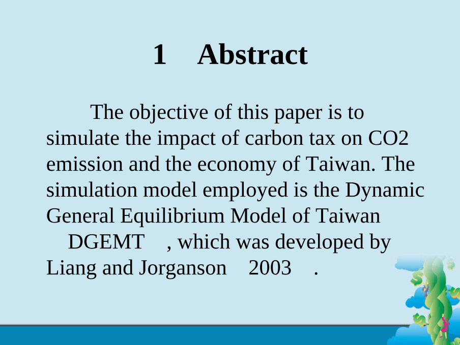
1、Abstract

The objective of this paper is to simulate the impact of carbon tax on CO2 emission and the economy of Taiwan. The simulation model employed is the Dynamic General Equilibrium Model of Taiwan（DGEMT）, which was developed by Liang and Jorganson（2003）.

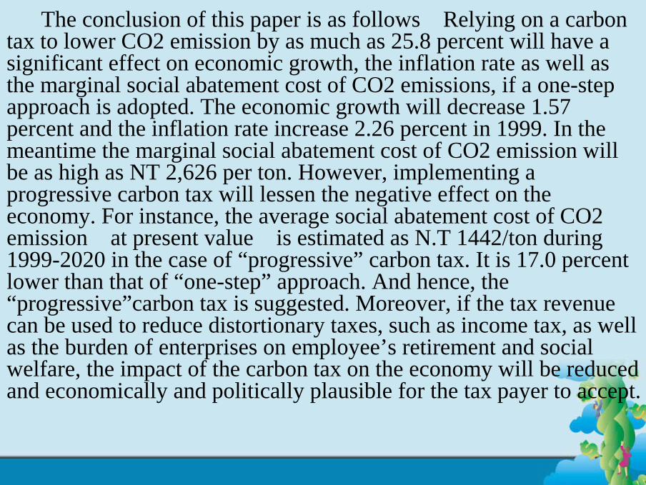
The conclusion of this paper is as follows：Relying on a carbon tax to lower CO2 emission by as much as 25.8 percent will have asignificant effect on economic growth, the inflation rate as well as the marginal social abatement cost of CO2 emissions, if a one-step approach is adopted. The economic growth will decrease 1.57 percent and the inflation rate increase 2.26 percent in 1999. In the meantime the marginal social abatement cost of CO2 emission willbe as high as NT 2,626 per ton. However, implementing a progressive carbon tax will lessen the negative effect on the economy. For instance, the average social abatement cost of CO2 emission（at present value）is estimated as N.T 1442/ton during 1999-2020 in the case of “progressive” carbon tax. It is 17.0 percent lower than that of “one-step” approach. And hence, the “progressive”carbon tax is suggested. Moreover, if the tax revenue can be used to reduce distortionary taxes, such as income tax, as well as the burden of enterprises on employee’s retirement and social welfare, the impact of the carbon tax on the economy will be reduced and economically and politically plausible for the tax payer to accept.

2、Introduction

Since February 16, 2005, the Kyoto protocol has been valid. Although Taiwan is not a member of ICPP, Taiwan has to respond to the Kyoto protocol actively, because if trade retaliation happened, the impact on Taiwan’s economy will be enormously. Taiwan’s degree of trade dependency （Sum of exports and imports／GDP）is very high. It was 105％ in 2003.

However, by 2003 CO2 emission for the economy as a whole had increased from 189.56 million ton in 1996 to 267.22 million ton, which is a 40.1 percent increase or 5.14 percent per annum during 1996-2003. It is noted that although the average GDP growth rate declined from 5.69 percent during 1996-1999 to 2.63 percent during 1999-2003 (See Table 1, col. 2), CO2 growth rate increased from 5.04 percent per annum to 5.24 percent per annum during 1999-2003 (See Table 1, col.1). As a result, the income elasticity of CO2 emission jumped from 0.88 during 1996-1999 to 2.00 during 1999-2003 (see Table 1, col. 3).

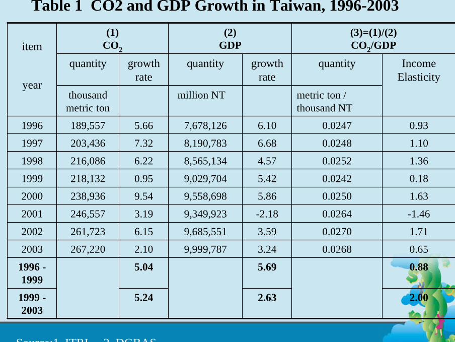
Table 1 CO2 and GDP Growth in Taiwan, 1996-2003

2.002.63 5.24 1999 -2003

0.885.69 5.04 1996 -1999

0.65 0.0268 3.249,999,7872.10 267,220 2003

1.71 0.0270 3.599,685,5516.15 261,723 2002

-1.46 0.0264 -2.189,349,9233.19 246,557 2001

1.63 0.0250 5.869,558,6989.54 238,936 2000

0.18 0.0242 5.429,029,7040.95 218,132 1999

1.36 0.0252 4.578,565,1346.22 216,086 1998

1.10 0.0248 6.688,190,7837.32 203,436 1997

0.93 0.0247 6.107,678,1265.66 189,557 1996

metric ton / thousand NT＄

％million NT＄％thousand metric ton

Income Elasticity

quantitygrowth rate

quantitygrowth rate

quantity

(3)=(1)/(2)CO2/GDP

(2)GDP

(1)CO2item

year

Source:1. ITRI 2. DGBAS

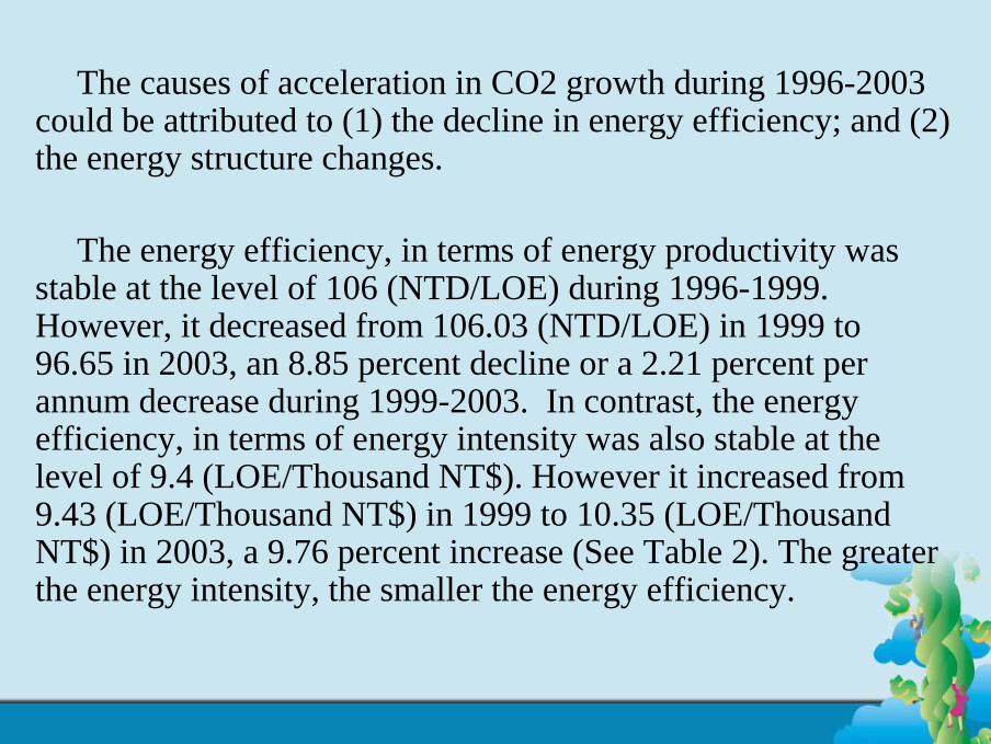
The causes of acceleration in CO2 growth during 1996-2003 could be attributed to (1) the decline in energy efficiency; and (2) the energy structure changes.

The energy efficiency, in terms of energy productivity was stable at the level of 106 (NTD/LOE) during 1996-1999. However, it decreased from 106.03 (NTD/LOE) in 1999 to 96.65 in 2003, an 8.85 percent decline or a 2.21 percent per annum decrease during 1999-2003. In contrast, the energy efficiency, in terms of energy intensity was also stable at the level of 9.4 (LOE/Thousand NT$). However it increased from 9.43 (LOE/Thousand NT$) in 1999 to 10.35 (LOE/Thousand NT$) in 2003, a 9.76 percent increase (See Table 2). The greaterthe energy intensity, the smaller the energy efficiency.

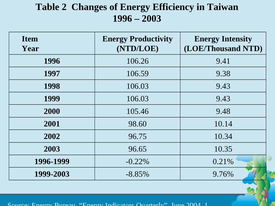
Table 2 Changes of Energy Efficiency in Taiwan 1996 – 2003

9.76%-8.85%1999-20030.21%-0.22%1996-199910.3596.65200310.3496.75200210.1498.6020019.48105.4620009.43106.0319999.43106.0319989.38106.5919979.41106.261996

Energy Intensity (LOE/Thousand NTD)

Energy Productivity (NTD/LOE)

ItemYear

Source: Energy Bureau, “Energy Indicators Quarterly”, June 2004. 1

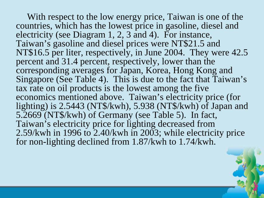
With respect to the low energy price, Taiwan is one of the countries, which has the lowest price in gasoline, diesel and electricity (see Diagram 1, 2, 3 and 4). For instance, Taiwan’s gasoline and diesel prices were NT$21.5 and NT$16.5 per liter, respectively, in June 2004. They were 42.5 percent and 31.4 percent, respectively, lower than the corresponding averages for Japan, Korea, Hong Kong and Singapore (See Table 4). This is due to the fact that Taiwan’s tax rate on oil products is the lowest among the five economics mentioned above. Taiwan’s electricity price (for lighting) is 2.5443 (NT$/kwh), 5.938 (NT$/kwh) of Japan and 5.2669 (NT$/kwh) of Germany (see Table 5). In fact, Taiwan’s electricity price for lighting decreased from 2.59/kwh in 1996 to 2.40/kwh in 2003; while electricity price for non-lighting declined from 1.87/kwh to 1.74/kwh.

Diagram 1 International Comparison on Gasoline Price

Gasoline

21.5

0

10

20

30

40

50

60

Indonesia

U.S.A.

Canada

Australia

Taiwan

Singapore

Greece

Japan

Luxemburg

Ireland

Austria

South Korean

Belgian

Switzerland

Netherlands

Hong Kong

Prices (NT$/L)

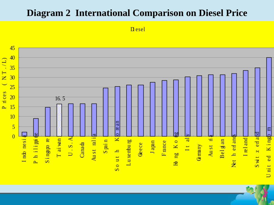
Diagram 2 International Comparison on Diesel PriceDiesel

16.5

0

5

10

15

20

25

30

35

40

45

Indonesia

Philippine

Singapore

Taiwan

U.S.A.

Canada

Australia

Spain

South Korean

Luxemburg

Greece

Japan

France

Hong Kong

Italy

Germany

Austria

Belgian

Netherlands

Ireland

Switzerland

United Kingdom

Prices (N.T./L)

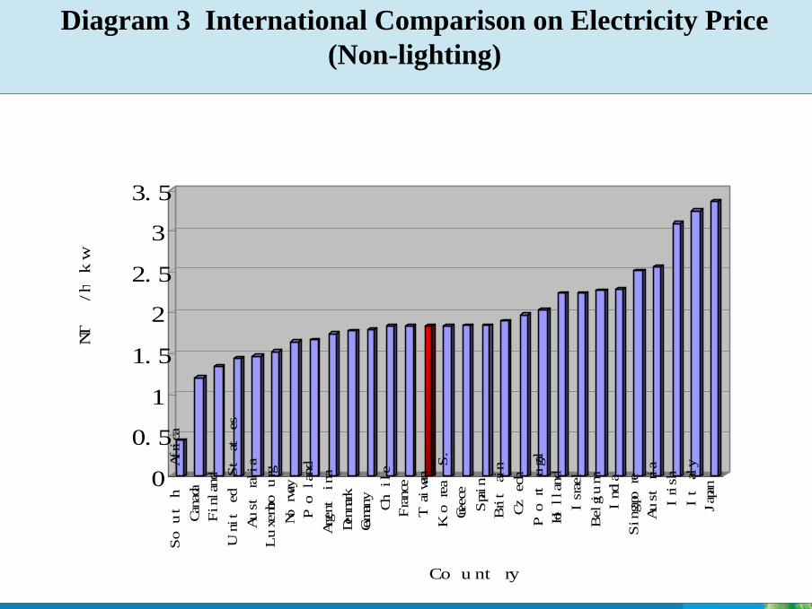
Diagram 3 International Comparison on Electricity Price (Non-lighting)

0

0.5

1

1.5

2

2.5

3

3.5

NT / kw

h

South Africa

Canada

Finland

United States

Australia

Luxembourg

Norway

Poland

Argentina

Denmark

Germany

Chile

France

Taiwan

Korea S.

Greece

Spain

Britain

Czech

Portugal

Holland

Israel

Belgium

India

Singapore

Austria

Irish

Italy

Japan

Country

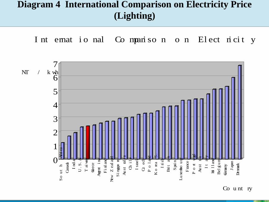
Diagram 4 International Comparison on Electricity Price (Lighting)

0

1

2

3

4

5

6

7NT / kwh

South Africa

Canada

India

U.S.A.

Taiwan

Greece

Argentina

Finland

New Zealand

Singapore

Australia

Chile

Israel

Czech

Poland

Korea S.

Irish

Britain

Spain

Luxembourg

France

Portugal

Austria

Italy

Holland

Belgium

Germany

Japan

Denmark

Country

International Comparison on Electricity Price (Lighting)

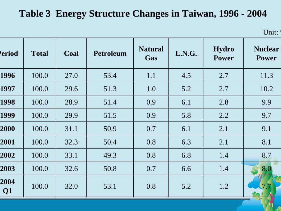
Table 3 Energy Structure Changes in Taiwan, 1996 - 2004

7.71.25.20.853.132.0100.02004 Q1

8.01.46.60.750.832.6100.02003

8.71.46.80.849.333.1100.02002

8.12.16.30.850.432.3100.02001

9.12.16.10.750.931.1100.02000

9.72.25.80.951.529.9100.01999

9.92.86.10.951.428.9100.01998

10.22.75.21.051.329.6100.01997

11.32.74.51.153.427.0100.01996

Nuclear Power

Hydro PowerL.N.G.Natural

GasPetroleumCoalTotalPeriod

Unit: %

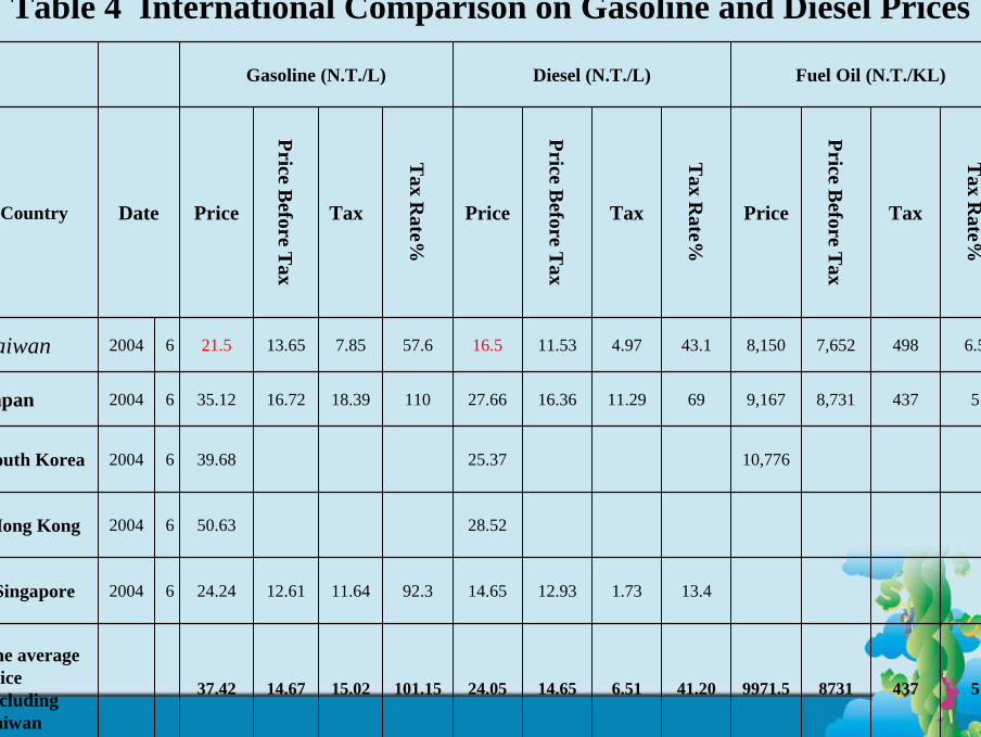
Table 4 International Comparison on Gasoline and Diesel Prices

543787319971.541.206.5114.6524.05101.1515.0214.6737.42

The average price excluding Taiwan

13.41.7312.9314.6592.311.6412.6124.2462004Singapore

28.5250.6362004Hong Kong

10,77625.3739.6862004South Korea

54378,7319,1676911.2916.3627.6611018.3916.7235.1262004Japan

6.54987,6528,15043.14.9711.5316.557.67.8513.6521.562004Taiwan

Tax R

ate%

Tax

Price Before T

ax

Price

Tax R

ate%

Tax

Price Before T

ax

Price

Tax R

ate%

Tax

Price Before T

ax

PriceDateCountry

Fuel Oil (N.T./KL)Diesel (N.T./L)Gasoline (N.T./L)

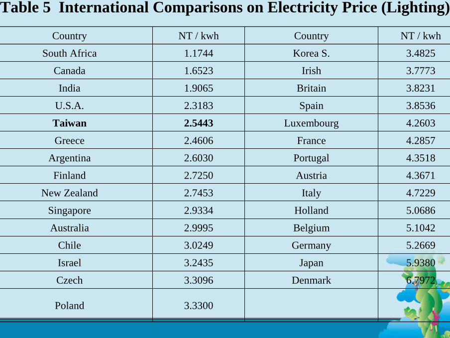
Table 5 International Comparisons on Electricity Price (Lighting)

3.3300Poland

6.7972Denmark 3.3096Czech

5.9380Japan 3.2435Israel

5.2669Germany 3.0249Chile

5.1042Belgium 2.9995Australia

5.0686Holland 2.9334Singapore

4.7229Italy 2.7453New Zealand

4.3671Austria 2.7250Finland

4.3518Portugal 2.6030Argentina

4.2857France 2.4606Greece

4.2603Luxembourg 2.5443Taiwan

3.8536Spain 2.3183U.S.A.

3.8231Britain 1.9065India

3.7773Irish 1.6523Canada

3.4825Korea S. 1.1744South Africa

NT / kwhCountryNT / kwhCountry

It is pertinent for Taiwan to upwardly adjust its energy prices via higher energy-related taxes, such as carbon tax, in order to conserve energy consumption and reduce the social costs associated with energy consumption, that arise due to air pollution, CO2 emissions, traffic congestion and instability of energy supply. However, whether the implementation of carbon tax is plausible or not depends on a precise evaluation of the effect of the taxes on energy conservation and the economy.

Since a high carbon tax might have a significant impact on the economy, a step-by-step or ‘progressive’approach should be examined as an alternative. Therefore, once it is decided to implement a carbon tax, the next question will be that of determining the best approach, i.e. a ‘one step’ approach or a ‘progressive’approach, that should be adopted. The selection will depend on a comparison of the carbon tax effects of a ‘one step’ approach and a ‘progressive’ approach on CO2 emissions and the economy.

The purpose of this paper is therefore to evaluate and compare the effect of a carbon tax on the price level, output growth and CO2emissions by sector and for the economy as a whole by applying the ‘one-step’ approach as well as the ‘progressive’ approach during the 1999-2020 period. Policy recommendations are drawn from the findings.

The paper consists of the following four sections: (1) Introduction; (2) The Theoretical Model; (3) The Simulation Methodology and Procedure; (4) Simulation Results; and (5) Conclusion.

For the evaluation of the carbon tax on Taiwan’s economy, please refer to Liang (2000).

3、The Theoretical Model Dynamic Generalized Equilibrium Model of Taiwan

The dynamic generalized equilibrium model of Taiwan (DGEMT) consists of the following four sub-models:

(1) the producer’s model; (2) the consumer’s model; (3) the DGBAS’s macroeconomic model; and (4) ITRI’s MARKAL engineering energy model.

3.1 Producer’s ModelThe producer’s model decomposes the Taiwan economy into

twenty-nine sectors, namely, eight main sectors (including agriculture, mining, manufacturing, construction, public utilities, transportation, services and industry (mining, manufacturing, construction and public utilities)), seventeen manufacturing sectors (including food, beverages & tobacco, textiles, clothes & wearing apparel, leather & leather products,wood & bamboo products, furniture products, paper & printing, chemicals & plastics, rubber products, non-metallic minerals, basic metals, metal products, machinery & equipment, electrical machinery & electronics, transportation equipment and miscellaneous), and four energy sectors (including coal mining, oil refining, natural gas and electricity).

We assume that the sectoral cost function is of the translog form with homothetic weak separability of energy and material inputs. The model actually consists of four sub-models (for each sector): an aggregate sub-model, an energy sub-model, a non-energy intermediate input sub-model, and an oil product sub-model. The aggregate sub-model includes one output price equation and five equations relating to the cost shares of capital, labor, energy, non-energy intermediate inputs and the rate of technological change. The energy sub-model has one price (energy price) equation and four share equations explaining the cost shares of coal, oil products, natural gas, and electricity, respectively.

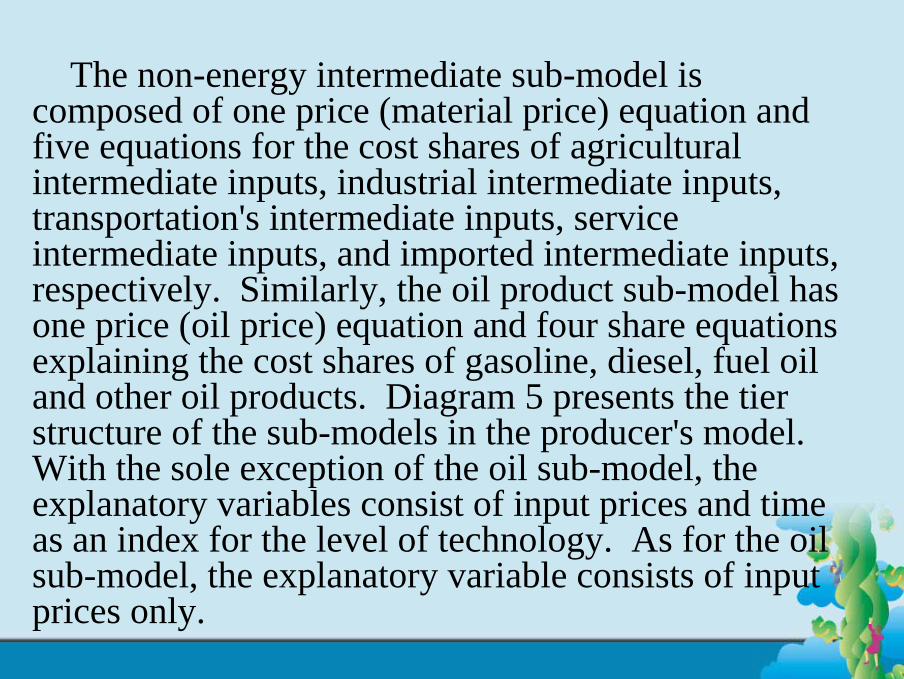
The non-energy intermediate sub-model is composed of one price (material price) equation and five equations for the cost shares of agricultural intermediate inputs, industrial intermediate inputs, transportation's intermediate inputs, service intermediate inputs, and imported intermediate inputs, respectively. Similarly, the oil product sub-model has one price (oil price) equation and four share equations explaining the cost shares of gasoline, diesel, fuel oil and other oil products. Diagram 5 presents the tier structure of the sub-models in the producer's model. With the sole exception of the oil sub-model, the explanatory variables consist of input prices and time as an index for the level of technology. As for the oil sub-model, the explanatory variable consists of input prices only.

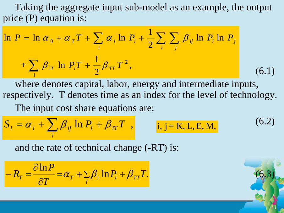
Taking the aggregate input sub-model as an example, the output price (P) equation is:

(6.1)where denotes capital, labor, energy and intermediate inputs,

respectively. T denotes time as an index for the level of technology.The input cost share equations are:

(6.2)

and the rate of technical change (-RT) is:

(6.3)

,21ln+

lnln21lnlnln

i

2

0

∑

∑ ∑ ∑

+

+++=

TTP

PPPTP

TTiiT

i i jjiijiiT

ββ

βααα

∑ ++=i

iTiijii TPS , ln ββα M, E, L, K,=j i,

.lnln TPT

PR TTi

iiTT ββα ++=∂∂

=− ∑

The basic approach of the model, which is a modification of the Hudson-Jorgenson (1974) model, is an integration of econometric modeling and input-output analysis. However, to reflect the dramatic changes in both the industrial structure and energy consumption patterns of the Taiwan economy, a time trend is included in the energy and material sub-models. This innovation makes this Jorgenson-Liang (1985) model significantly different from most of the studies by Jorgenson and his associates, which are based on highly-developed economies, such as the United States, Japan and West Germany. This kind of model will be also useful for case studies involving the other newly industrializing countries (NICs).

Liang (1987), Jorgenson and Liang (1985) and Liang (1999) contain detailed descriptions of this theoretical model, together with the estimation method, data compilation and the results of coefficients estimated. It is noted that Liang (1999) is a revised model of Jorgenson-Liang (1985) in that it updates the time-series data of the producer’s model from 1961-1981 to 1961-1993, and also combines the consumer’s model (Liang (1983)), the macroeconomic model of the Directorate-General of Budget, Accounting and Statistics, Executive Yuan (Ho-Lin-Wang (2001)), and the MARKAL Engineering Model of the Industrial Technology Research Institute (Young (1996)).

3.2 The Consumer’s Model

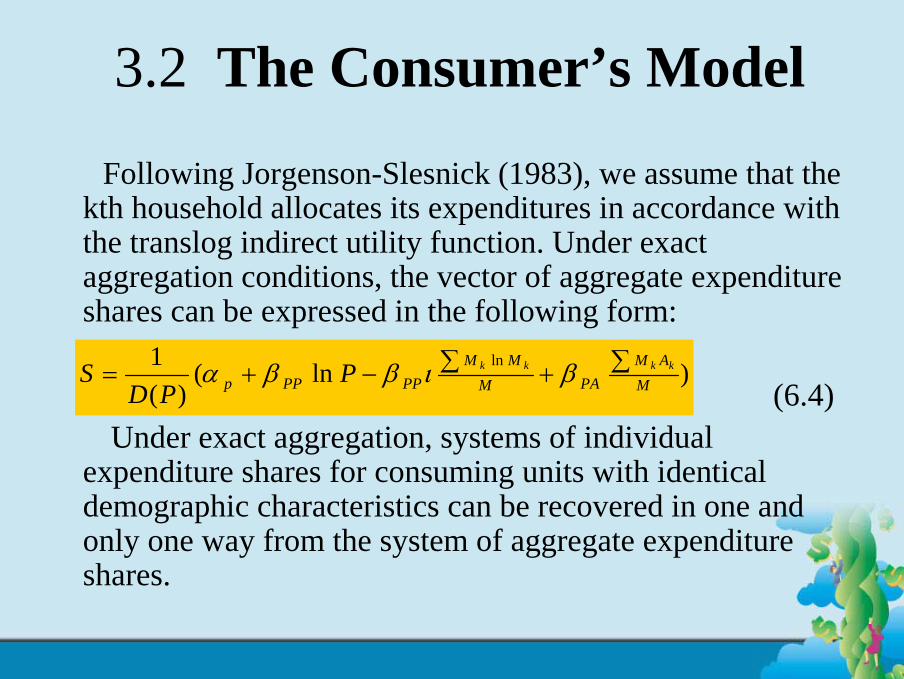
Following Jorgenson-Slesnick (1983), we assume that the kth household allocates its expenditures in accordance with the translog indirect utility function. Under exact aggregation conditions, the vector of aggregate expenditure shares can be expressed in the following form:

(6.4)Under exact aggregation, systems of individual

expenditure shares for consuming units with identical demographic characteristics can be recovered in one and only one way from the system of aggregate expenditure shares.

)ln()(

1 lnM

AMPAM

MMPPPPp

kkkkPPD

S ∑+∑−+= βιββα

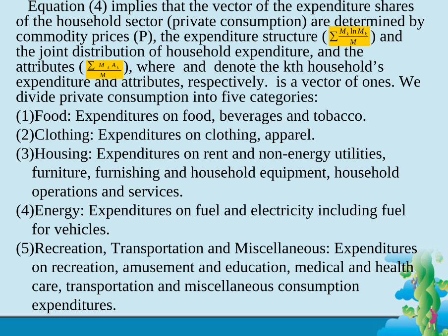
Equation (4) implies that the vector of the expenditure shares of the household sector (private consumption) are determined by commodity prices (P), the expenditure structure ( ) and the joint distribution of household expenditure, and the attributes ( ), where and denote the kth household’s expenditure and attributes, respectively. is a vector of ones. We divide private consumption into five categories: (1)Food: Expenditures on food, beverages and tobacco.(2)Clothing: Expenditures on clothing, apparel.(3)Housing: Expenditures on rent and non-energy utilities,

furniture, furnishing and household equipment, household operations and services.

(4)Energy: Expenditures on fuel and electricity including fuel for vehicles.

(5)Recreation, Transportation and Miscellaneous: Expenditures on recreation, amusement and education, medical and health care, transportation and miscellaneous consumptionexpenditures.

∑ MMM kk ln

MAM kk∑

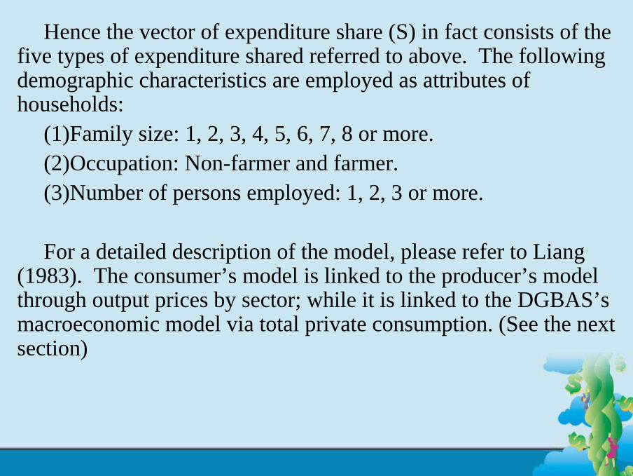
Hence the vector of expenditure share (S) in fact consists of the five types of expenditure shared referred to above. The following demographic characteristics are employed as attributes of households:

(1)Family size: 1, 2, 3, 4, 5, 6, 7, 8 or more.(2)Occupation: Non-farmer and farmer.(3)Number of persons employed: 1, 2, 3 or more.

For a detailed description of the model, please refer to Liang (1983). The consumer’s model is linked to the producer’s model through output prices by sector; while it is linked to the DGBAS’smacroeconomic model via total private consumption. (See the nextsection)

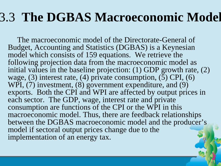
3.3 The DGBAS Macroeconomic ModelThe macroeconomic model of the Directorate-General of

Budget, Accounting and Statistics (DGBAS) is a Keynesian model which consists of 159 equations. We retrieve the following projection data from the macroeconomic model as initial values in the baseline projection: (1) GDP growth rate, (2) wage, (3) interest rate, (4) private consumption, (5) CPI, (6) WPI, (7) investment, (8) government expenditure, and (9) exports. Both the CPI and WPI are affected by output prices in each sector. The GDP, wage, interest rate and private consumption are functions of the CPI or the WPI in this macroeconomic model. Thus, there are feedback relationships between the DGBAS macroeconomic model and the producer’s model if sectoral output prices change due to the implementation of an energy tax.

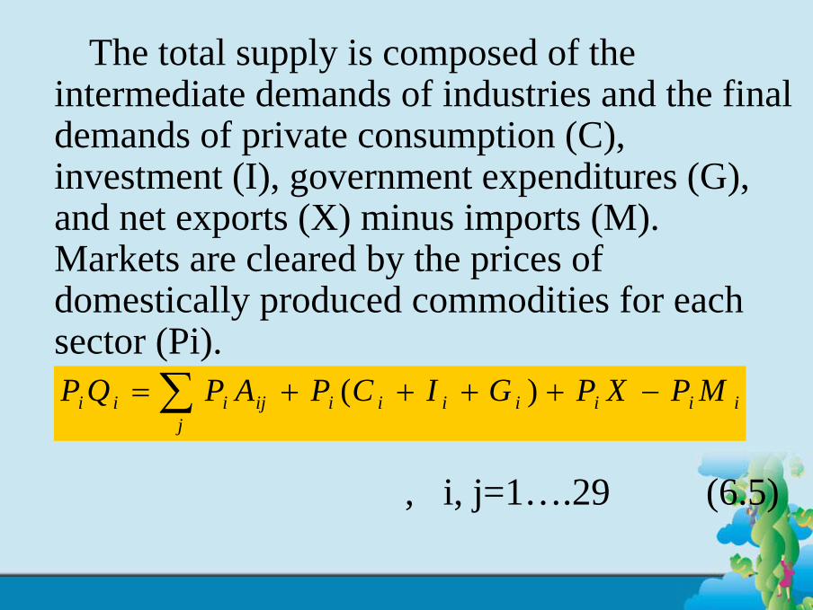
The total supply is composed of the intermediate demands of industries and the final demands of private consumption (C), investment (I), government expenditures (G), and net exports (X) minus imports (M). Markets are cleared by the prices of domestically produced commodities for each sector (Pi).

, i, j=1….29 (6.5)

iiiiiiiijj

iii MPXPGICPAPQP −++++= ∑ )(

3.4 The ITRI MARKAL Engineering Energy Model

By employing the linear programming method, the ITRI MARKAL engineering model combines the information relating to the growth of industries, energy supply and energy technologies to achieve the best energy mix. This model is developed by the Institute for Energy and Resources of the Industrial Technology Research Institute (ITRI).

Because information regarding future energy technology development is given careful consideration in the model, we use the aggregate of the energy demand by types projected by the ITRI MARKAL engineering model to control for the total energy demand projected by the producer’s and consumer’s models.

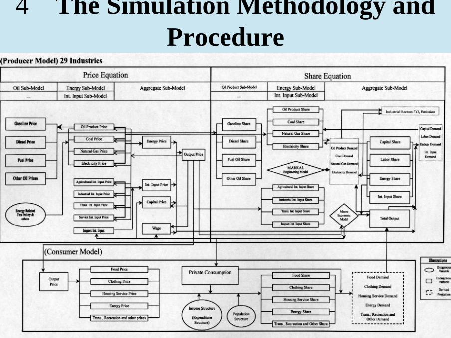
4、The Simulation Methodology and Procedure

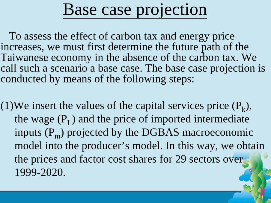
Base case projectionTo assess the effect of carbon tax and energy price

increases, we must first determine the future path of the Taiwanese economy in the absence of the carbon tax. We call such a scenario a base case. The base case projection is conducted by means of the following steps:

(1)We insert the values of the capital services price (Pk), the wage (PL) and the price of imported intermediate inputs (Pm) projected by the DGBAS macroeconomic model into the producer’s model. In this way, we obtain the prices and factor cost shares for 29 sectors over 1999-2020.

(2)By employing the 1996 input-output table, we then convert the 29 sectoral output prices into the prices of 5 consumer goods during 1999-2020. By inserting the prices of 5 consumer goods together with the private consumption as projected by the macroeconomic model into the consumer’s model, we obtain the shares of 5 consumer goods in total private consumption.

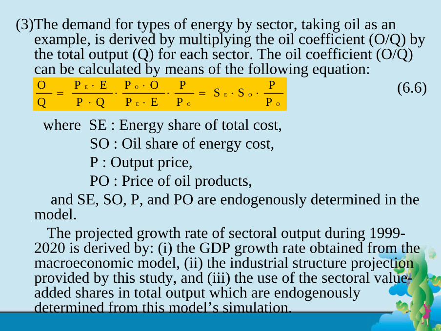
(3)The demand for types of energy by sector, taking oil as an example, is derived by multiplying the oil coefficient (O/Q) by the total output (Q) for each sector. The oil coefficient (O/Q) can be calculated by means of the following equation:

(6.6)

where SE : Energy share of total cost,SO : Oil share of energy cost,P : Output price,PO : Price of oil products,

and SE, SO, P, and PO are endogenously determined in the model.

The projected growth rate of sectoral output during 1999-2020 is derived by: (i) the GDP growth rate obtained from the macroeconomic model, (ii) the industrial structure projection provided by this study, and (iii) the use of the sectoral value-added shares in total output which are endogenously determined from this model’s simulation.

OQ

P EP Q

P OP E

PP

S S PP

E O

E O

E O

O

=⋅⋅

⋅⋅⋅

⋅ = ⋅ ⋅

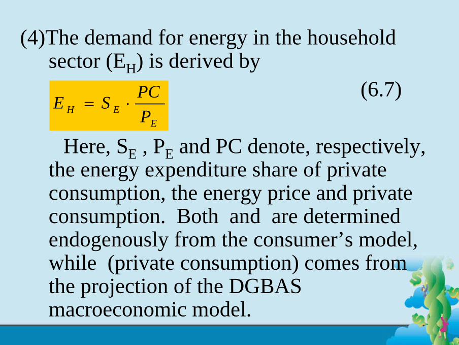
(4)The demand for energy in the household sector (EH) is derived by

(6.7)

Here, SE , PE and PC denote, respectively, the energy expenditure share of private consumption, the energy price and private consumption. Both and are determined endogenously from the consumer’s model, while (private consumption) comes from the projection of the DGBAS macroeconomic model.

EEH P

PCSE ⋅=

(5)The demand for the various types of energy are then converted into CO2 emissions by employing the conversion factor projected by the MARKAL engineering model, such as: coal (3.53 tons CO2/KLOE), oil products (2.89 tons CO2/KLOE), and natural gas (2.09 tons CO2/KLOE). This completes the whole process of baseline projection.

Simulation Involving Carbon Tax and Energy Price Increases

(6)Next, we evaluate the impact of carbon tax and energy price increases. We convert the prices of different energy types ranging from endogenous to exogenous. The prices of energy are modified by incorporating energy tax schedules into the producer’s model and consumer’s model, respectively, to calculate their corresponding output prices, cost shares, demand for types of energy and CO2 emissions by sectors, as well as the consumption structure and quantity of consumer goods.

(7)However, the above scenarios do not consider the ‘feedback’ effect in the changes in the capital service price (PK), wage (PL) and output caused by implementing the tax. In fact, the implementation of carbon tax will affect PK and PL and total output by sector as well. In the DGBAS macroeconomic model, PK and PL are affected by the carbon tax through the increase in the general price level. Hence we insert the GDP deflator into the PK and PL function to obtain a new PK and PL, and in turn new values of the output price, cost structure and CO2 emissions by sector.

(8)The impact of the carbon tax on total output by sector is evaluated by means of the following procedure:

(a) First of all, we calculate the impact of the carbon tax on the sectoral output price and the general price level (GDP deflator), and, in turn, the new values of final demand such as private consumption, investment, government expenditure, net exports and GDP.

(b) Next, we multiply the private consumption by the private consumption shares of the five consumer goods, which are then deflated by their respective prices to obtain the new values of the five consumer goods.

(c) We then employ the 1996 Input-Output table to convert the changes in the five consumer goods to the changes in sectoral final demand (FD).

(d) We obtain the sectoral total output (Q) by using the following standard input-output equation Here, D denotes the matrix of domestic product input-output coefficients.

(e) We calculate the energy conservation effect on the total output of the four energy sectors and the whole economy. The energy conservation effect is obtained by comparing the demand for the four types of energy in the base case with that in the carbon tax case where carbon tax are implemented.

(9)Finally, the impact of carbon tax on the sectoral output price, the demand for various types of energy and CO2 emissions are compared.

It is noted that the imposition of carbon tax and energy price increase will reduce total output and further reduce the demand for energy and CO2 emission. Therefore, the total impact of carbon tax and energy price increase on CO2 emissions reduction should also accommodate the effect on output growth. In a nutshell, we consider not only the ‘substitution effect’ but also the

‘income effect,’ both in the consumer’s and producer’s models, in relation to the demand for energy and CO2 emissions.

5、The Simulation Results

5.1 Effect of Carbon Tax on PricesThe carbon tax schedule for Holland

(US$2.24/tons CO2), Finland (US$3.93/tons CO2), Denmark (US$14.88/tons CO2) and Sweden (US$ 22.2/tons CO2), which are shown in Table 6. Among these, oil has the highest tax rate, followed by fuel oil, LPG, natural gas, diesel oil, gasoline and electricity.

Because there is not perfect substitutability among the different types of energy (e.g., coal and fuel oil cannot replace gasolineand diesel for car use) and the tax rate of each kind of energy is different, the unit caloric prices of various types of energy are different in Taiwan. The present unit caloric energy price structure is as follows (take the unit caloric price of coal as 1) coal: premium gasoline: premium diesel: fuel oil: LPG: natural gas: electricity = 1: 4.25: 2.68: 0.84: 1.58: 1.63: 4.29.

By imposing the carbon tax rate and taking the US$22.2/tons CO2 tax rate as an example, the energy price structure (in NT$/LOE) will be changed to coal: premium gasoline: premium diesel: fuel oil: LPG: natural gas: electricity = 1: 3.0: 2.0: 0.83: 1.26: 1.25: 2.97 (see Table 6). After imposing the carbon tax, each energy price related to coal declines significantly except for fuel oil. This brings advantages to natural gas, electricity and LPG that may serve as substitutes for coal and fuel oil in the producer’s sector (see Table 6).

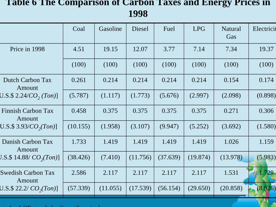
Table 6 The Comparison of Carbon Taxes and Energy Prices in 1998

(8.926) (20.858) (29.650) (56.154) (17.539) (11.055) (57.339)

1.7291.5312.1172.1172.1172.1172.586Swedish Carbon Tax Amount

[U.S.$ 22.2/ CO2(Ton)]

(5.983) (13.978) (19.874) (37.639) (11.756) (7.410) (38.426)

1.1591.0261.4191.4191.4191.4191.733Danish Carbon Tax Amount

[U.S.$ 14.88/ CO2(Ton)]

(1.580) (3.692) (5.252) (9.947) (3.107) (1.958) (10.155)

0.3060.2710.3750.3750.3750.3750.458Finnish Carbon Tax Amount

[U.S.$ 3.93/CO2(Ton)]

(0.898) (2.098) (2.997) (5.676) (1.773) (1.117) (5.787)

0.1740.1540.2140.2140.2140.2140.261Dutch Carbon Tax Amount

[U.S.$ 2.24/CO2 (Ton)]

(100)(100)(100)(100)(100)(100)(100)

19.377.347.143.7712.0719.154.51Price in 1998

ElectricityNatural Gas

LPGFuelDieselGasolineCoal

Note 1：LOE stands for liter oil equivalent.

5.2 Effect of Carbon Tax —A One-Step Approach

Effect on Energy Demand and CO2 Emissions

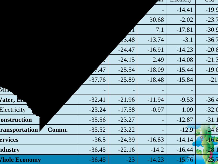
By imposing the highest carbon tax (U.S.$22.2/CO2 (Ton)) through the use of a one-step approach, CO2 emissions decrease by 25.77 percent for the economy as a whole in 1999. The energy demand in relation to coal has the largest decrease, which is –36.45 percent, followed by oil products –23 percent, natural gas –14.23 percent and electricity –15.76 percent (see Table 7).

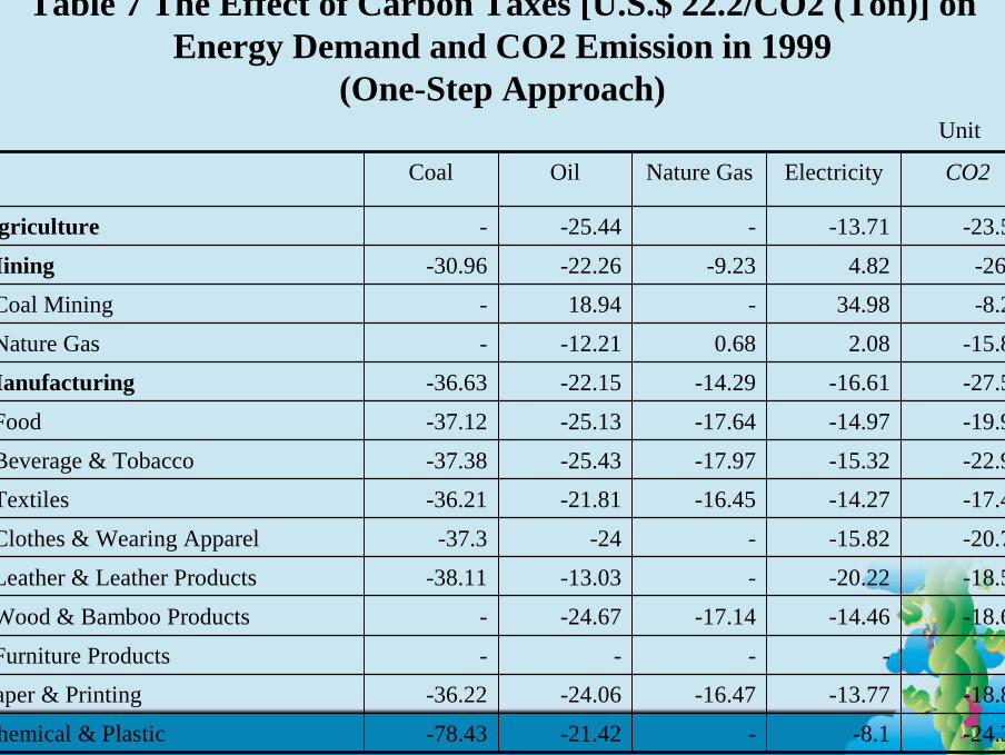
Table 7 The Effect of Carbon Taxes [U.S.$ 22.2/CO2 (Ton)] on Energy Demand and CO2 Emission in 1999

(One-Step Approach)

-24.31-8.1--21.42-78.43Chemical & Plastic

-18.87-13.77-16.47-24.06-36.22Paper & Printing

-----Furniture Products

-18.64-14.46-17.14-24.67-Wood & Bamboo Products

-18.57-20.22--13.03-38.11Leather & Leather Products

-20.75-15.82--24-37.3Clothes & Wearing Apparel

-17.42-14.27-16.45-21.81-36.21Textiles

-22.98-15.32-17.97-25.43-37.38Beverage & Tobacco

-19.99-14.97-17.64-25.13-37.12Food

-27.53-16.61-14.29-22.15-36.63Manufacturing

-15.852.080.68-12.21-Nature Gas

-8.2534.98-18.94-Coal Mining

-26.94.82-9.23-22.26-30.96Mining

-23.58-13.71--25.44-Agriculture

CO2ElectricityNature GasOilCoal

Unit：%

CO2ElectricityNature GasOilCoal

--25.7725.77-15.76-14.23-23-36.45Whole Economy-28.18-16.44-14.2-22.16-36.45Industry-16.48-14.14-16.83-24.39-36.5Services-24.88-12.9--23.22-35.52Transportation ＆ Comm.-31.17-12.87--23.27-35.56Construction-32.081.09-0.97-17.58-23.24Electricity-36.45-9.53-11.94-21.96-32.41Water, Electricity ＆ Gas

-----Miscellaneous-21.2-15.84-18.48-25.89-37.76Transport Equipment

-19.05-15.44-18.09-25.54-37.47Elect. Mach. & Electronics-21.33-14.082.49-24.15-36.29Machinery & Equipment-20.83-14.23-16.91-24.47-36.56Metal Products-36.71-3.1-13.74-13.48-52.59Basic Metal-30.96-17.817.1-23.11-34.97Non-Metallic Mineral-23.75-2.0230.68-0.44-15.95Oil Refinery-19.97-14.41--24.72-36.72Rubber Products

Effect on Output Prices:

Imposing an energy tax will of course have the greatest impact on the prices within the four energy sectors (see Table 8). Among manufacturing industries, the non-metallic mineral products, basic metal and chemical products industries will suffer the greatest impact in terms of price increases. Public utilities and transportation will have the highest price increases among the seven one-digit sectors. For the economy as a whole, the GDP deflator will increase by 2.26 percent in 1999, if the highest energy tax rate of U.S$22.2/CO2 (Ton) is imposed (see Table 8).

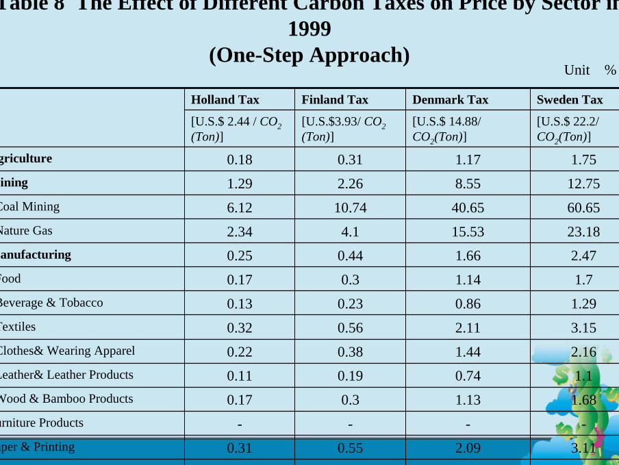
Table 8 The Effect of Different Carbon Taxes on Price by Sector in 1999

(One-Step Approach)

3.672.460.650.37Chemical & Plastic

3.112.090.550.31Paper & Printing

----Furniture Products

1.681.130.30.17Wood & Bamboo Products

1.10.740.190.11Leather& Leather Products

2.161.440.380.22Clothes& Wearing Apparel

3.152.110.560.32Textiles

1.290.860.230.13Beverage & Tobacco

1.71.140.30.17Food

2.471.660.440.25Manufacturing

23.1815.534.12.34Nature Gas

60.6540.6510.746.12Coal Mining

12.758.552.261.29Mining

1.751.170.310.18Agriculture

[U.S.$ 22.2/ CO2(Ton)]

[U.S.$ 14.88/ CO2(Ton)]

[U.S.$3.93/ CO2 (Ton)]

[U.S.$ 2.44 / CO2(Ton)]

Sweden TaxDenmark TaxFinland TaxHolland Tax

Unit：%

[U.S.$ 22.2/ CO2(Ton)]

[U.S.$ 14.88/ CO2(Ton)][U.S.$3.93/ CO2 (Ton)]

[U.S.$ 2.44 / CO2(Ton)]

Sweden TaxDenmark TaxFinland TaxHolland Tax

2.262.261.520.400.23GDP Deflator

3.592.410.640.36Industry

1.270.850.230.13Services

4.382.930.780.44Transportation ＆ Comm.

2.81.880.50.28Construction

19.3712.983.431.95Electricity

16.1610.832.861.63Water, Electricity＆Gas

1.841.230.330.19Miscellaneous

1.551.040.270.16Transport Equipment

1.20.80.210.12Elect. Mach. & Electronics

2.151.440.380.22Machinery & Equipment

2.581.730.460.26Metal Products

4.162.790.740.42Basic Metal

5.113.430.910.52Non-Metallic Mineral

35.3123.676.253.56Oil Refinery

2.321.560.410.23Rubber Products

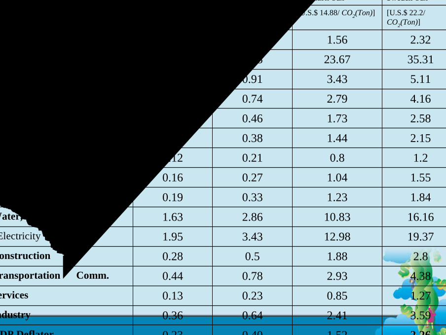
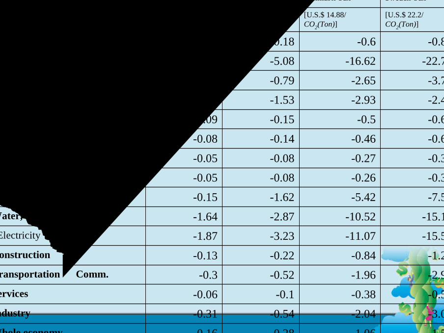
Effect on Output Growth

The four energy sectors will also suffer the greatest decline in output growth when the energy tax is imposed. This is due to the‘substitution effect’ and ‘income effect’ both in terms of the final demand and the producer’s sector. Similarly, the non-metallic mineral products, basic metal and chemical products sectors are among the most affected parts of the manufacturing sector. The public utility and transportation sectors will exhibit the greatest decrease in output growth among the seven one-digit sectors. For the economy as a whole, GDP will decline by 1.57 percent if the highest energy tax rate U.S$22.2/CO2 (Ton) is imposed (see Table 9).

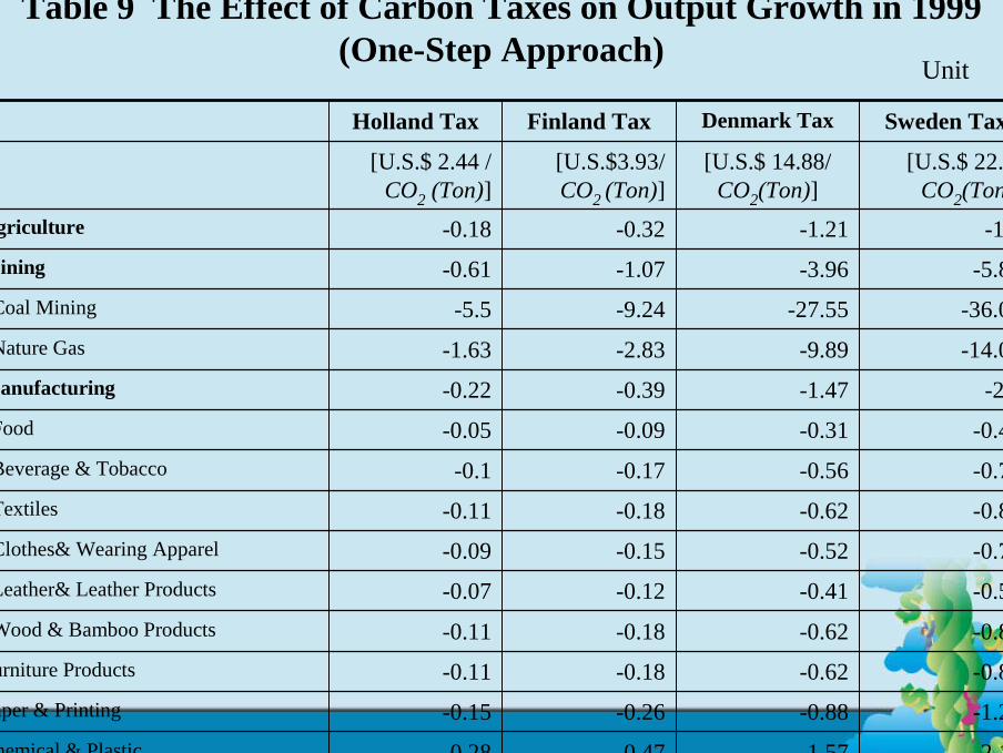
Table 9 The Effect of Carbon Taxes on Output Growth in 1999(One-Step Approach)

-2.19-1.57-0.47-0.28Chemical & Plastic

-1.23-0.88-0.26-0.15Paper & Printing

-0.86-0.62-0.18-0.11Furniture Products

-0.87-0.62-0.18-0.11Wood & Bamboo Products

-0.58-0.41-0.12-0.07Leather& Leather Products

-0.72-0.52-0.15-0.09Clothes& Wearing Apparel

-0.87-0.62-0.18-0.11Textiles

-0.78-0.56-0.17-0.1Beverage & Tobacco

-0.43-0.31-0.09-0.05Food

-2.2-1.47-0.39-0.22Manufacturing

-14.07-9.89-2.83-1.63Nature Gas

-36.04-27.55-9.24-5.5Coal Mining

-5.83-3.96-1.07-0.61Mining

-1.8-1.21-0.32-0.18Agriculture

[U.S.$ 22.2/ CO2(Ton)]

[U.S.$ 14.88/ CO2(Ton)]

[U.S.$3.93/ CO2 (Ton)]

[U.S.$ 2.44 / CO2 (Ton)]

Sweden TaxDenmark TaxFinland TaxHolland Tax

Unit：％

[U.S.$ 22.2/ CO2(Ton)]

[U.S.$ 14.88/ CO2(Ton)]

[U.S.$3.93/ CO2 (Ton)]

[U.S.$ 2.44 / CO2(Ton)]

Sweden TaxDenmark TaxFinland TaxHolland Tax

-1.57-1.06-0.28-0.16Whole economy

-3.01-2.04-0.54-0.31Industry

-0.56-0.38-0.1-0.06Services

-2.92-1.96-0.52-0.3Transportation ＆ Comm.

-1.26-0.84-0.22-0.13Construction

-15.58-11.07-3.23-1.87Electricity

-15.13-10.52-2.87-1.64Water, Electricity ＆ Gas

-7.58-5.42-1.62-0.15Miscellaneous

-0.36-0.26-0.08-0.05Transport Equipment

-0.37-0.27-0.08-0.05Elect. Mach. & Electronics

-0.64-0.46-0.14-0.08Machinery & Equipment

-0.69-0.5-0.15-0.09Metal Products

-2.49-2.93-1.53-0.96Basic Metal

-3.71-2.65-0.79-0.46Non-Metallic Mineral

-22.74-16.62-5.08-2.97Oil Refinery

-0.84-0.6-0.18-0.1Rubber Products

5.3 Effect of Carbon Tax –A Progressive Approach

Alternatively, we might choose a progressive approach to achieve the same goal of CO2 reduction, while minimizing its impact on the economy. Using a progressive ad valorem tax approach, we assume that the tax rate in 2020 is the same as that when a one-step approach is used in 1999. The schedule for the 22-year progressive ad valorem tax rate is presented in Table 10.

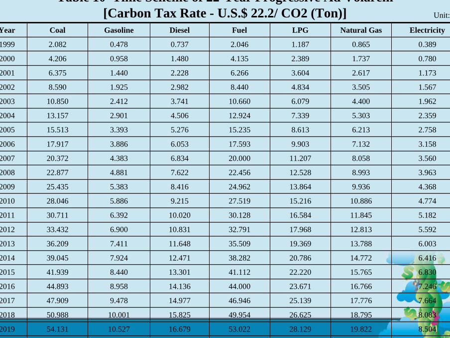
Table 10 Time Scheme of 22-Year Progressive Ad Volarem[Carbon Tax Rate - U.S.$ 22.2/ CO2 (Ton)] Unit: %

8.926 20.858 29.650 56.154 17.539 11.055 57.339 2020

8.504 19.822 28.129 53.022 16.679 10.527 54.131 2019

8.083 18.795 26.625 49.954 15.825 10.001 50.988 2018

7.664 17.776 25.139 46.946 14.977 9.478 47.909 2017

7.246 16.766 23.671 44.000 14.136 8.958 44.893 2016

6.830 15.765 22.220 41.112 13.301 8.440 41.939 2015

6.416 14.772 20.786 38.282 12.471 7.924 39.045 2014

6.003 13.788 19.369 35.509 11.648 7.411 36.209 2013

5.592 12.813 17.968 32.791 10.831 6.900 33.432 2012

5.182 11.845 16.584 30.128 10.020 6.392 30.711 2011

4.774 10.886 15.216 27.519 9.215 5.886 28.046 2010

4.368 9.936 13.864 24.962 8.416 5.383 25.435 2009

3.963 8.993 12.528 22.456 7.622 4.881 22.877 2008

3.560 8.058 11.207 20.000 6.834 4.383 20.372 2007

3.158 7.132 9.903 17.593 6.053 3.886 17.917 2006

2.758 6.213 8.613 15.235 5.276 3.393 15.513 2005

2.359 5.303 7.339 12.924 4.506 2.901 13.157 2004

1.962 4.400 6.079 10.660 3.741 2.412 10.850 2003

1.567 3.505 4.834 8.440 2.982 1.925 8.590 2002

1.173 2.617 3.604 6.266 2.228 1.440 6.375 2001

0.780 1.737 2.389 4.135 1.480 0.958 4.206 2000

0.389 0.865 1.187 2.046 0.737 0.478 2.082 1999

ElectricityNatural GasLPGFuelDieselGasolineCoalYear

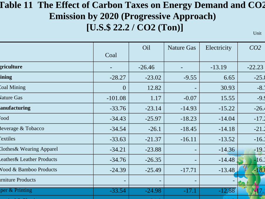
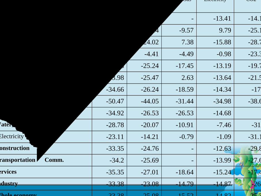
Table 11 The Effect of Carbon Taxes on Energy Demand and CO2 Emission by 2020 (Progressive Approach)

[U.S.$ 22.2 / CO2 (Ton)]Unit：%

-21.9-11.9--24.8-Chemical & Plastic

-17.11-12.88-17.1-24.98-33.54Paper & Printing

-----Furniture Products

-18.85-13.48-17.71-25.49-24.39Wood & Bamboo Products

-16.38-14.48--26.35-34.76Leather& Leather Products

-19.33-14.36--23.88-34.21Clothes& Wearing Apparel

-16.33-13.52-16.11-21.37-33.63Textiles

-21.26-14.18-18.45-26.1-34.54Beverage & Tobacco

-17.29-14.04-18.23-25.97-34.43Food

-26.44-15.22-14.93-23.14-33.76Manufacturing

-9.9515.55-0.071.17-101.08Nature Gas

-8.7830.93-12.820Coal Mining

-25.896.65-9.55-23.02-28.27Mining

-22.23-13.19--26.46-Agriculture

CO2ElectricityNature GasOilCoal

CO2ElectricityNature GasOilCoal

-25.31-14.82-15.52-25.08-33.38Whole economy

-26.9-14.87-14.79-23.08-33.38Industry

-17.44-15.24-18.64-27.01-35.35Services

-27.62-13.99--25.69-34.2Transportation ＆ Comm.

-29.85-12.63--24.76-33.35Construction

-31.17-1.09-0.79-14.21-23.11Electricity

-31.7-7.46-10.91-20.07-28.78Water, Electricity ＆ Gas

--14.68-26.53-26.53-34.92Miscellaneous

-38.66-34.98-31.44-44.05-50.47Transport Equipment

-17.8-14.34-18.59-26.24-34.66Elect. Mach. & Electronics

-21.59-13.642.63-25.47-33.98Machinery & Equipment

-19.76-13.19-17.45-25.24-33.78Metal Products

-23.38-0.98-4.49-4.41-35.32Basic Metal

-28.74-15.887.38-24.02-32.46Non-Metallic Mineral

-25.169.79-9.570.14-11.93Oil Refinery

-14.15-13.41---27.09Rubber Products

Effect on Energy Demand and CO2 Emissions

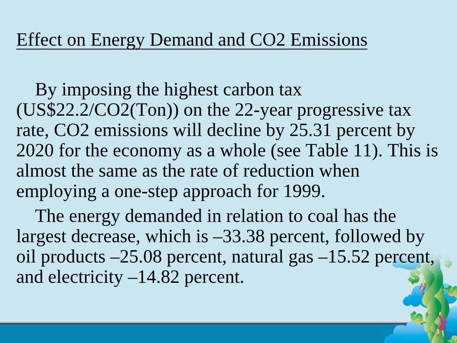
By imposing the highest carbon tax (US$22.2/CO2(Ton)) on the 22-year progressive tax rate, CO2 emissions will decline by 25.31 percent by 2020 for the economy as a whole (see Table 11). This is almost the same as the rate of reduction when employing a one-step approach for 1999.

The energy demanded in relation to coal has the largest decrease, which is –33.38 percent, followed by oil products –25.08 percent, natural gas –15.52 percent, and electricity –14.82 percent.

Effect on Prices

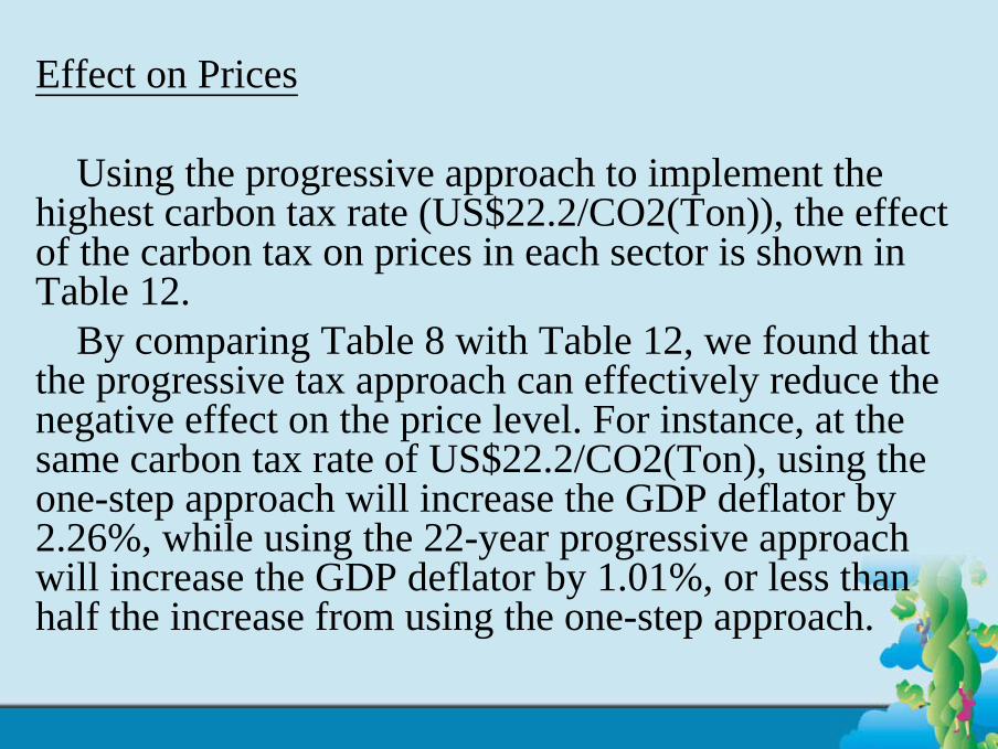
Using the progressive approach to implement the highest carbon tax rate (US$22.2/CO2(Ton)), the effect of the carbon tax on prices in each sector is shown in Table 12.

By comparing Table 8 with Table 12, we found that the progressive tax approach can effectively reduce the negative effect on the price level. For instance, at the same carbon tax rate of US$22.2/CO2(Ton), using the one-step approach will increase the GDP deflator by 2.26%, while using the 22-year progressive approach will increase the GDP deflator by 1.01%, or less than half the increase from using the one-step approach.

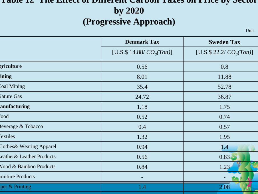
Table 12 The Effect of Different Carbon Taxes on Price by Sector by 2020

(Progressive Approach)Unit：％

2.571.74Chemical & Plastic

2.081.4Paper & Printing

--Furniture Products

1.230.84Wood & Bamboo Products

0.830.56Leather& Leather Products

1.40.94Clothes& Wearing Apparel

1.951.32Textiles

0.570.4Beverage & Tobacco

0.740.52Food

1.751.18Manufacturing

36.8724.72Nature Gas

52.7835.4Coal Mining

11.888.01Mining

0.80.56Agriculture

[U.S.$ 22.2/ CO2(Ton)][U.S.$ 14.88/ CO2(Ton)]

Sweden TaxDenmark Tax

[U.S.$ 22.2/ CO2(Ton)][U.S.$ 14.88/ CO2(Ton)]

Sweden TaxDenmark Tax

1.010.69GDP Deflator

2.761.86Industry

--Services

1.120.85Transportation ＆ Comm.

1.791.22Construction

16.9911.42Electricity

14.429.67Water, Electricity ＆ Gas

1.470.98Miscellaneous

0.960.65Transport Equipment

0.720.5Elect. Mach. & Electronics

1.380.93Machinery & Equipment

1.721.17Metal Products

3.392.28Basic Metal

3.722.48Non-Metallic Mineral

35.5823.85Oil Refinery

1.51.02Rubber Products

By imposing the 22-year progressive approach, the water, electricity and gas sector (14.42%) is affected the most in terms of a price increase among the seven one-digit sectors. It is followed by mining (11.88%), construction (1.79%), manufacturing (1.75%), transportation (1.12%) and agriculture (0.80%). The top five manufacturing sectors in terms of respective price increases are oil refining (35.58%), non-metallic minerals (3.72%), basic metals (3.39%), chemicals and plastics (2.57%) and paper & printing (2.08%).

To sum up, sectoral ranking in terms of the impact of price increases as a result of imposing the 22-year progressive carbon tax is identical with the case where the one-step carbon tax is used (see Tables 12 and 8).

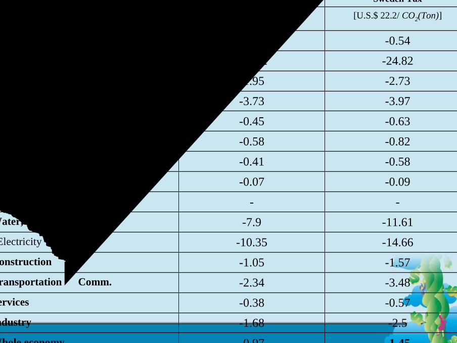
Effect on Output Growth

By comparing Table 13 with Table 9, we conclude that, when the 22-year progressive carbon tax is imposed, GDP will be reduced by 1.45 percent by 2020, which is less than the reduction from using a one-step approach (-1.57 percent). Similarly, the sectoral ranking in terms of the decrease in output as a result of imposing the 22-year progressive carbon tax is also the same as that in the case of the one-step carbon tax.

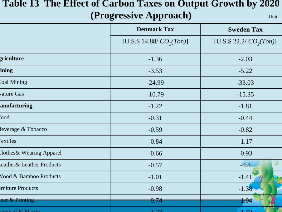
Table 13 The Effect of Carbon Taxes on Output Growth by 2020(Progressive Approach) Unit：％

-1.72-1.23Chemical & Plastic

-1.04-0.74Paper & Printing

-1.38-0.98Furniture Products

-1.41-1.01Wood & Bamboo Products

-0.8-0.57Leather& Leather Products

-0.93-0.66Clothes& Wearing Apparel

-1.17-0.84Textiles

-0.82-0.59Beverage & Tobacco

-0.44-0.31Food

-1.81-1.22Manufacturing

-15.35-10.79Nature Gas

-33.03-24.99Coal Mining

-5.22-3.53Mining

-2.03-1.36Agriculture

[U.S.$ 22.2/ CO2(Ton)][U.S.$ 14.88/ CO2(Ton)]

Sweden TaxDenmark Tax

[U.S.$ 22.2/ CO2(Ton)][U.S.$ 14.88/ CO2(Ton)]

Sweden TaxDenmark Tax

-1.45-0.97Whole economy

-2.5-1.68Industry

-0.57-0.38Services

-3.48-2.34Transportation ＆ Comm.

-1.57-1.05Construction

-14.66-10.35Electricity

-11.61-7.9Water, Electricity ＆ Gas

--Miscellaneous

-0.09-0.07Transport Equipment

-0.58-0.41Elect. Mach. & Electronics

-0.82-0.58Machinery & Equipment

-0.63-0.45Metal Products

-3.97-3.73Basic Metal

-2.73-1.95Non-Metallic Mineral

-24.82-18.12Oil Refinery

-0.54-0.39Rubber Products

Marginal Social Abatement Cost of CO2 Emissions

Here, we define the marginal social abatement cost of CO2 emissions as the change in GDP divided by the change in CO2 emissions. The figures denoting the changes in both GDP and CO2 emissions are derived from various scenarios related to the carbon tax schemes mentioned above.

Table 14 present the marginal social abatement cost of CO2 reductions by employing various tax rate in 1999. We find that the marginal social abatement cost rises significantly with the increase in the targeted CO2 reduction. For instance, when the targeted CO2 reduction increases from 3.48 percent to 25.77 percent, the marginal social abatement cost will increase from NT$1,982/ton to NT$2,626/ton in 1999, a 25.50 percent increase.

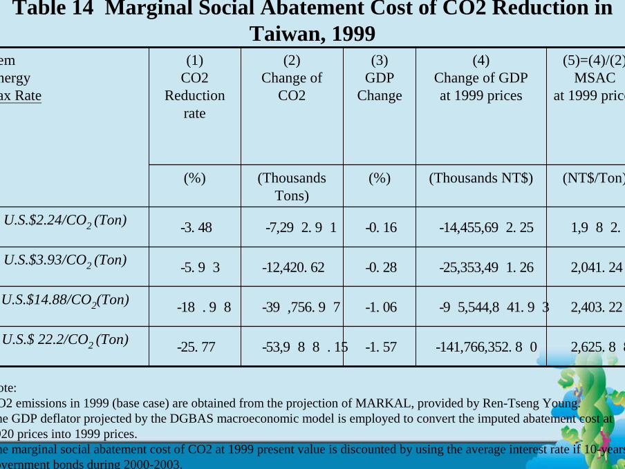
Table 14 Marginal Social Abatement Cost of CO2 Reduction in Taiwan, 1999

2,625.88-141,766,352.80-1.57-53,988.15-25.77U.S.$ 22.2/CO2 (Ton)

2,403.22-95,544,841.93-1.06-39,756.97-18.98U.S.$14.88/CO2(Ton)

2,041.24-25,353,491.26-0.28-12,420.62-5.93U.S.$3.93/CO2 (Ton)

1,982.16-14,455,692.25-0.16-7,292.91-3.48U.S.$2.24/CO2 (Ton)

(NT$/Ton)(Thousands NT$)(%)(Thousands Tons)

(%)

(5)=(4)/(2)MSAC

at 1999 prices

(4)Change of GDPat 1999 prices

(3)GDP

Change

(2)Change of

CO2

(1)CO2

Reduction rate

ItemEnergyTax Rate

Note:CO2 emissions in 1999 (base case) are obtained from the projection of MARKAL, provided by Ren-Tseng Young.The GDP deflator projected by the DGBAS macroeconomic model is employed to convert the imputed abatement cost at 2020 prices into 1999 prices.The marginal social abatement cost of CO2 at 1999 present value is discounted by using the average interest rate if 10-years government bonds during 2000-2003.

To compare the abatement cost of CO2 emission by using “one-step” and “progressive” approach, a time path analysis is required. First, we estimate the impact of carbon tax on CO2 emission and GDP year by year during 1999-2020. Second, a 5.38 percent discounted rate, which is the average government bond rate (ten years) during 1995-2003, is employed to discount the change of GDP at 1999 constant prices to the present value.

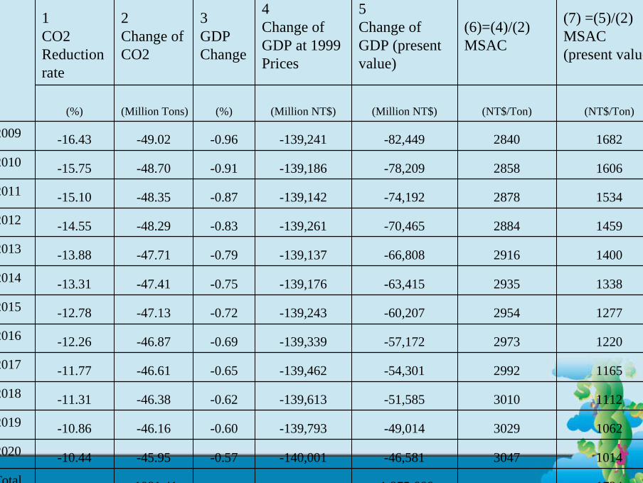
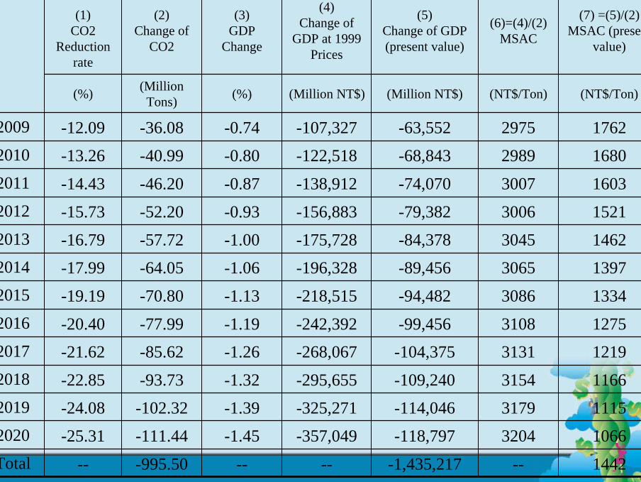
Taking the highest tax rate of (US$22.2/CO2(Ton)) as an example, Table 15 and Table 16 present marginal social abatement cost of CO2 reduction during 1999-2020 by adopting “one-step” approach and “progressive” approach respectively.

We conclude that the average of marginal social abatement cost of CO2 reduction during 1999-2020 is NT$1,442 per ton by “progressive” approach, which is a 16.8 percent lower than that of “one-step” approach (NT$1,734 per ton). (See Table 15 and 16)

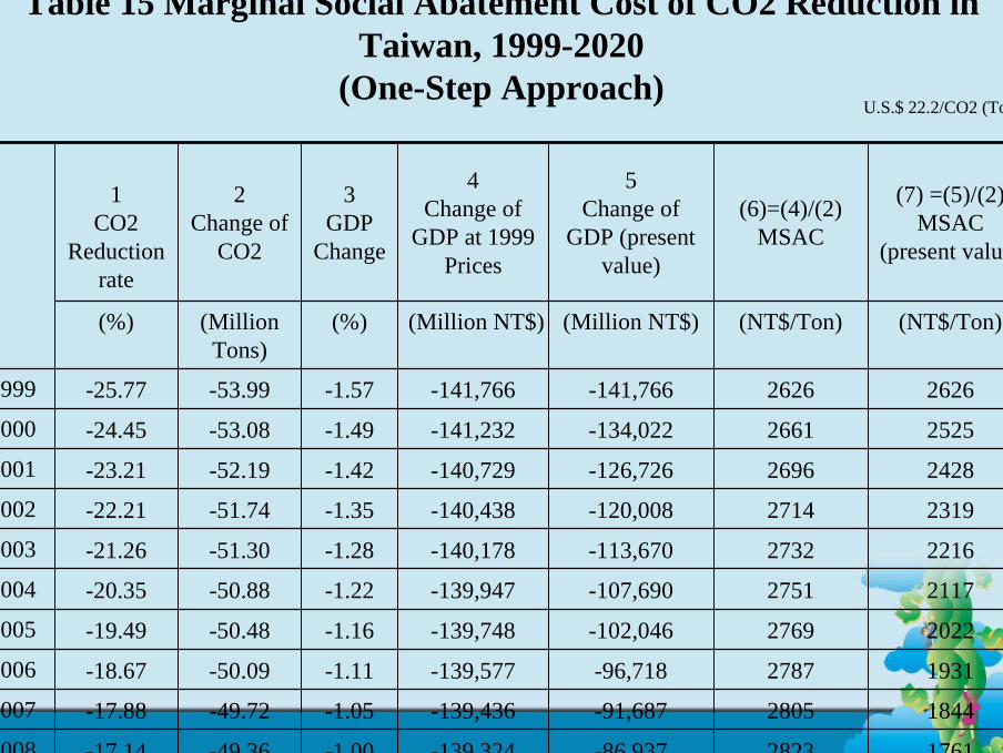
Table 15 Marginal Social Abatement Cost of CO2 Reduction in Taiwan, 1999-2020

(One-Step Approach)U.S.$ 22.2/CO2 (Ton)

17612823-86,937-139,324-1.00-49.36-17.142008

18442805-91,687-139,436-1.05-49.72-17.882007

19312787-96,718-139,577-1.11-50.09-18.672006

20222769-102,046-139,748-1.16-50.48-19.492005

21172751-107,690-139,947-1.22-50.88-20.352004

22162732-113,670-140,178-1.28-51.30-21.262003

23192714-120,008-140,438-1.35-51.74-22.212002

24282696-126,726-140,729-1.42-52.19-23.212001

25252661-134,022-141,232-1.49-53.08-24.452000

26262626-141,766-141,766-1.57-53.99-25.771999

(NT$/Ton)(NT$/Ton)(Million NT$)(Million NT$)(%)(Million Tons)

(%)

(7) =(5)/(2)MSAC

(present value)

(6)=(4)/(2)MSAC

5Change of

GDP (present value)

4Change of

GDP at 1999 Prices

3GDP

Change

2Change of

CO2

1CO2

Reduction rate

(NT$/Ton)(NT$/Ton)(Million NT$)(Million NT$)(%)(Million Tons)(%)

(7) =(5)/(2)MSAC (present value)

(6)=(4)/(2)MSAC

5Change of GDP (present value)

4Change of GDP at 1999 Prices

3GDP Change

2Change of CO2

1CO2 Reduction rate

1734---1,875,666-----1081.41--Total

10143047-46,581-140,001-0.57-45.95-10.442020

10623029-49,014-139,793-0.60-46.16-10.862019

11123010-51,585-139,613-0.62-46.38-11.312018

11652992-54,301-139,462-0.65-46.61-11.772017

12202973-57,172-139,339-0.69-46.87-12.262016

12772954-60,207-139,243-0.72-47.13-12.782015

13382935-63,415-139,176-0.75-47.41-13.312014

14002916-66,808-139,137-0.79-47.71-13.882013

14592884-70,465-139,261-0.83-48.29-14.552012

15342878-74,192-139,142-0.87-48.35-15.102011

16062858-78,209-139,186-0.91-48.70-15.752010

16822840-82,449-139,241-0.96-49.02-16.432009

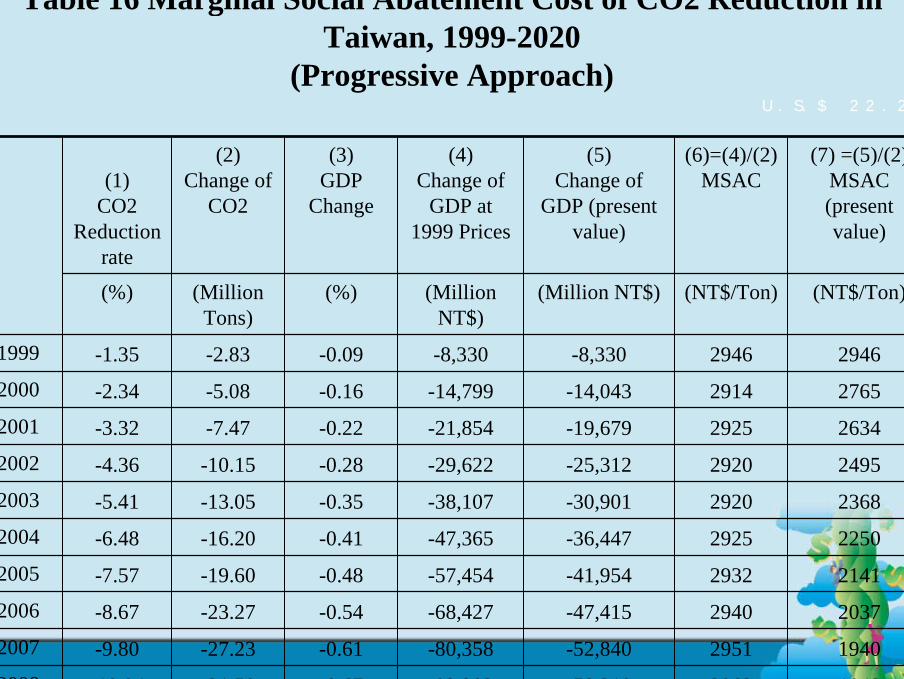
Table 16 Marginal Social Abatement Cost of CO2 Reduction in Taiwan, 1999-2020

(Progressive Approach)U.S.$ 22.2/CO2 (Ton)

18482962-58,219-93,302-0.67-31.50-10.942008

19402951-52,840-80,358-0.61-27.23-9.802007

20372940-47,415-68,427-0.54-23.27-8.672006

21412932-41,954-57,454-0.48-19.60-7.572005

22502925-36,447-47,365-0.41-16.20-6.482004

23682920-30,901-38,107-0.35-13.05-5.412003

24952920-25,312-29,622-0.28-10.15-4.362002

26342925-19,679-21,854-0.22-7.47-3.322001

27652914-14,043-14,799-0.16-5.08-2.342000

29462946-8,330-8,330-0.09-2.83-1.351999

(NT$/Ton)(NT$/Ton)(Million NT$)(Million NT$)

(%)(Million Tons)

(%)

(7) =(5)/(2)MSAC (present value)

(6)=(4)/(2)MSAC

(5)Change of

GDP (present value)

(4)Change of

GDP at 1999 Prices

(3)GDP

Change

(2)Change of

CO2(1)

CO2 Reduction

rate

(NT$/Ton)(NT$/Ton)(Million NT$)(Million NT$)(%)(Million Tons)(%)

(7) =(5)/(2)MSAC (present

value)

(6)=(4)/(2)MSAC

(5)Change of GDP (present value)

(4)Change of

GDP at 1999 Prices

(3)GDP

Change

(2)Change of

CO2

(1)CO2

Reduction rate

1442---1,435,217-----995.50--Total10663204-118,797-357,049-1.45-111.44-25.31202011153179-114,046-325,271-1.39-102.32-24.08201911663154-109,240-295,655-1.32-93.73-22.85201812193131-104,375-268,067-1.26-85.62-21.62201712753108-99,456-242,392-1.19-77.99-20.40201613343086-94,482-218,515-1.13-70.80-19.19201513973065-89,456-196,328-1.06-64.05-17.99201414623045-84,378-175,728-1.00-57.72-16.79201315213006-79,382-156,883-0.93-52.20-15.73201216033007-74,070-138,912-0.87-46.20-14.43201116802989-68,843-122,518-0.80-40.99-13.26201017622975-63,552-107,327-0.74-36.08-12.092009

6、Conclusion and Policy Suggestions

From the above findings, we conclude that relying on a carbon tax to lower CO2 emissions by as much as 25 percent will have a significant effect on economic growth, the inflation rate as well as the marginal social abatement cost of CO2 emissions, if a one-step approach is applied. However, implementing a ‘progressive’energy tax will lessen the negative effect on the economy. Consequently, it is recommended that the ‘progressive’ energy tax approach instead of the ‘one step’ energy tax approach be adopted.

It is recognized that the effect of tax revenue is not discussed here. In fact, this paper implicitly assumes that the tax revenue is used to reduce the government deficit. If the tax revenue can beused to reduce distortionary taxes elsewhere in the economy, such as income tax, the impact of the carbon tax on the economy will be reduced. This deserves further study in the future.