Embed Size (px)
Citation preview

THE EFFECT OF CHANGES IN MONETARY POLICY AND BALANCE OF
PAYMENT ON EXCHANGE RATES IN KENYA
MARTIN MURIITHI KABUTU
D61/68308/2011
A RESEARCH PROJECT SUBMITTED IN PARTIAL FULFILMENT OF THE
REQUIREMENT FOR THE DEGREE OF MASTER OF BUSINESS
ADMINISTRATION, SCHOOL OF BUSINESS, UNIVERSITY OF NAIROBI
OCTOBER 2015
ii
DECLARATION
I declare that this is my original work and has not been submitted at any academic institution
for examination purposes.
Signed........................... Date....................
MARTIN MURIITHI KABUTU
D61/68308/2011
This research project has been submitted for presentation with my approval as the university
supervisor.
Signed............................................. Date.......................
MR. HERICK ONDIGO
Lecturer, Department of Finance & Accounting
School of Business
University of Nairobi

iii
ACKNOWLEDGMENTS
It has been an exciting and instructive study period in the University of Nairobi and I feel
privileged to have had the opportunity to carry out this study as a demonstration of knowledge
gained during the period studying for my master‘s degree. With these acknowledgments, it
would be impossible not to remember those who in one way or another, directly or indirectly,
have played a role in the realization of this research project. Let me, therefore, thank them all
equally.
First, I am indebted to the all-powerful GOD for all the blessings he showered on me and for
being with me throughout the study. I am deeply obliged to my supervisor Mr. Herrick Ondigo
for his exemplary guidance and support without whose help; this project would not have been a
success. Finally, yet importantly, I take this opportunity to express my deep gratitude to my
loving family, and friends who are a constant source of motivation and for their never ending
support and encouragement during this project.

iv
DEDICATION
This project is dedicated to my family members. May the Almighty God bless you abundantly

v
TABLE OF CONTENTS
DECLARATION........................................................................................................................... ii
ACKNOWLEDGEMENTS ........................................................ Error! Bookmark not defined.
DEDICATION.............................................................................. Error! Bookmark not defined.
LIST OF TABLES ..................................................................................................................... viii
LIST OF ABBREVIATIONS ..................................................................................................... ix
ABSTRACT ................................................................................................................................... x
CHAPTER ONE ........................................................................................................................... 1
INTRODUCTION......................................................................................................................... 1
1.1 Background of the Study .......................................................................................................... 1
1.1.1 Monetary Policy ................................................................................................................. 2
1.1.2 Balance of Payment ............................................................................................................ 3
1.1.3 Exchange Rate .................................................................................................................... 4
1.1.4 Effect of Changes in Monetary Policy and Balance of Payment on Exchange Rate ......... 6
1.1.5 Monetary Policy, Balance of Payment and Exchange Rate in Kenya ............................... 7
1.2 Research Problem ..................................................................................................................... 9
1.3 Objective of the Study ............................................................................................................ 11
1.4 Value of the Study .................................................................................................................. 11
CHAPTER TWO ........................................................................................................................ 13
LITERATURE REVIEW .......................................................................................................... 13
2.1Introduction .............................................................................................................................. 13
2.2 Theoretical Review ................................................................................................................. 13
2.2.1 Flow-Oriented Theory ...................................................................................................... 13
2.2.2 AA-DD Model.................................................................................................................. 14
2.2.3 Overshooting Model ......................................................................................................... 15
2.3 Determinants of Exchange Rate.............................................................................................. 15
vi
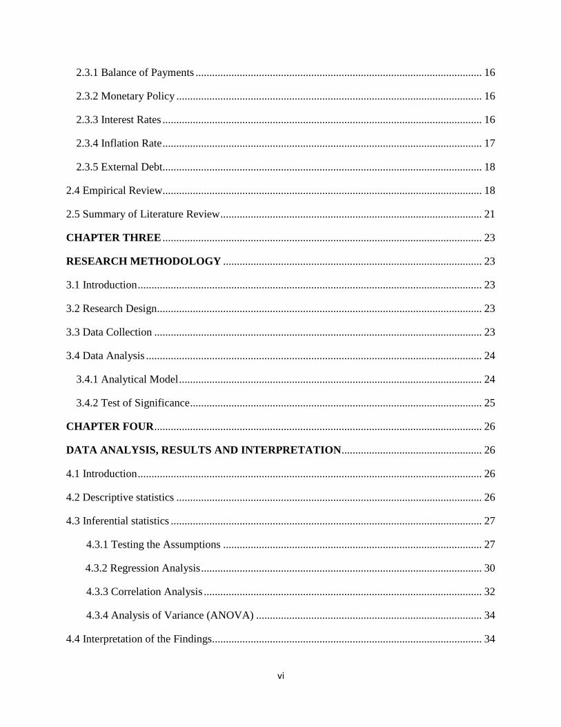
2.3.1 Balance of Payments ........................................................................................................ 16
2.3.2 Monetary Policy ............................................................................................................... 16
2.3.3 Interest Rates .................................................................................................................... 16
2.3.4 Inflation Rate .................................................................................................................... 17
2.3.5 External Debt.................................................................................................................... 18
2.4 Empirical Review.................................................................................................................... 18
2.5 Summary of Literature Review ............................................................................................... 21
CHAPTER THREE .................................................................................................................... 23
RESEARCH METHODOLOGY .............................................................................................. 23
3.1 Introduction ............................................................................................................................. 23
3.2 Research Design...................................................................................................................... 23
3.3 Data Collection ....................................................................................................................... 23
3.4 Data Analysis .......................................................................................................................... 24
3.4.1 Analytical Model .............................................................................................................. 24
3.4.2 Test of Significance .......................................................................................................... 25
CHAPTER FOUR ....................................................................................................................... 26
DATA ANALYSIS, RESULTS AND INTERPRETATION ................................................... 26
4.1 Introduction ............................................................................................................................. 26
4.2 Descriptive statistics ............................................................................................................... 26
4.3 Inferential statistics ................................................................................................................. 27
4.3.1 Testing the Assumptions .............................................................................................. 27
4.3.2 Regression Analysis ...................................................................................................... 30
4.3.3 Correlation Analysis ..................................................................................................... 32
4.3.4 Analysis of Variance (ANOVA) .................................................................................. 34
4.4 Interpretation of the Findings.................................................................................................. 34

vii
CHAPTER FIVE ........................................................................................................................ 36
SUMMARY, CONCLUSION AND RECOMMENDATIONS .............................................. 36
5.1 Introduction ............................................................................................................................. 36
5.2 Summary ................................................................................................................................. 36
5.3 Conclusion .............................................................................................................................. 38
5.4 Policy Recommendations........................................................................................................ 39
5.5 Limitations of the Study.......................................................................................................... 39
5.6 Suggestions for Further Research ........................................................................................... 39
REFERENCES ............................................................................................................................ 41
APPENDICES ............................................................................................................................. 45
APPENDIX I: Raw Data ........................................................................................................ 45
APPENDIX II: Output ............................................................................................................ 47
APPENDIX III: Exchange Rates Variance.............................................................................. 50
viii
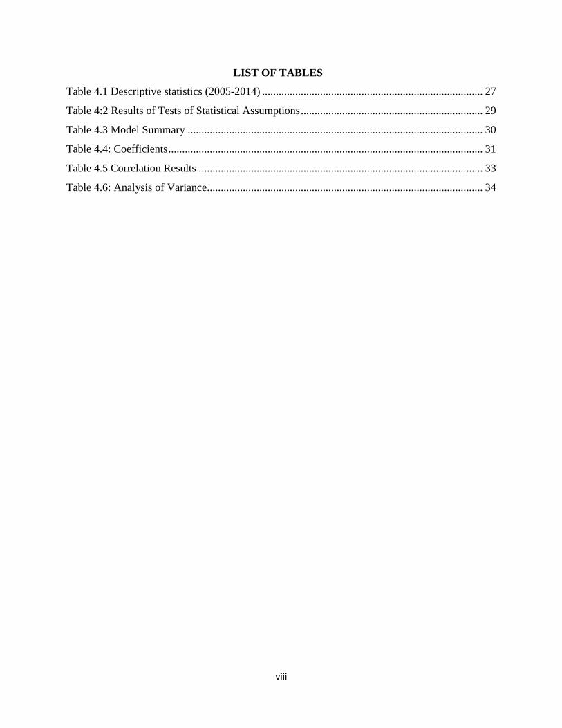
LIST OF TABLES
Table 4.1 Descriptive statistics (2005-2014) ................................................................................ 27
Table 4:2 Results of Tests of Statistical Assumptions .................................................................. 29
Table 4.3 Model Summary ........................................................................................................... 30
Table 4.4: Coefficients .................................................................................................................. 31
Table 4.5 Correlation Results ....................................................................................................... 33
Table 4.6: Analysis of Variance.................................................................................................... 34

ix
LIST OF ABBREVIATIONS
BOP - Balance of Payment
CBK - Central Bank of Kenya
CBII -Commercial Banks Intermediation Index
CBS -Central Bank of Syria
DR -Discount Rate
ERER -Equilibrium Real Exchange Rate
FX - Foreign Exchange
GDP -Gross Domestic Product
IMF -International Monetary Fund
INGOs -International Non-Governmental Organisations
KSH - Kenya Shilling
OMO -Open Market Operations
SDRs -Special Drawing Rights
RR -Reserve Requirement
USD - United States Dollar
VECM -Vector Error Correction Model
x
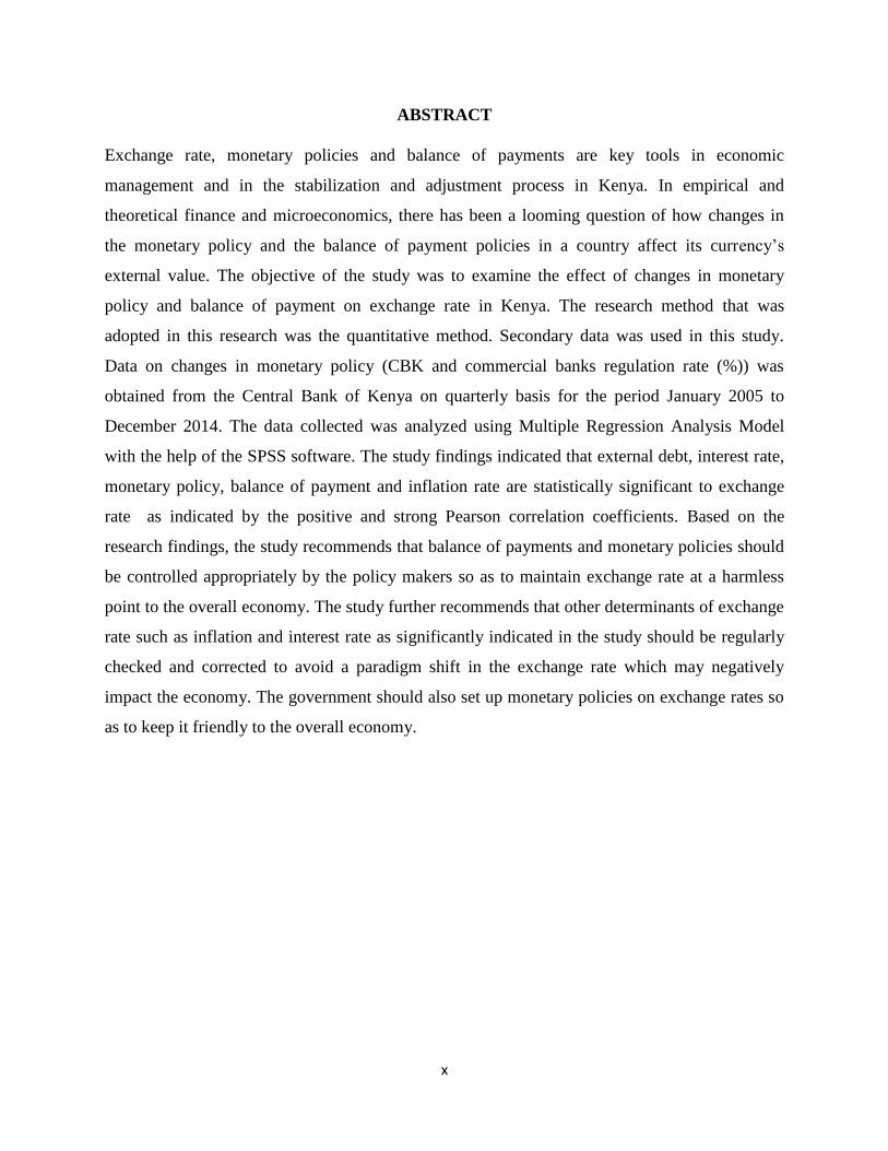
ABSTRACT
Exchange rate, monetary policies and balance of payments are key tools in economic
management and in the stabilization and adjustment process in Kenya. In empirical and
theoretical finance and microeconomics, there has been a looming question of how changes in
the monetary policy and the balance of payment policies in a country affect its currency‘s
external value. The objective of the study was to examine the effect of changes in monetary
policy and balance of payment on exchange rate in Kenya. The research method that was
adopted in this research was the quantitative method. Secondary data was used in this study.
Data on changes in monetary policy (CBK and commercial banks regulation rate (%)) was
obtained from the Central Bank of Kenya on quarterly basis for the period January 2005 to
December 2014. The data collected was analyzed using Multiple Regression Analysis Model
with the help of the SPSS software. The study findings indicated that external debt, interest rate,
monetary policy, balance of payment and inflation rate are statistically significant to exchange
rate as indicated by the positive and strong Pearson correlation coefficients. Based on the
research findings, the study recommends that balance of payments and monetary policies should
be controlled appropriately by the policy makers so as to maintain exchange rate at a harmless
point to the overall economy. The study further recommends that other determinants of exchange
rate such as inflation and interest rate as significantly indicated in the study should be regularly
checked and corrected to avoid a paradigm shift in the exchange rate which may negatively
impact the economy. The government should also set up monetary policies on exchange rates so
as to keep it friendly to the overall economy.

1
CHAPTER ONE
INTRODUCTION
1.1 Background of the Study
Over a long time now, there has been a raging debate on the effect on monetary policy and
balance of payment on exchange rate. In Kenya, various scholars in the economic and finance
front have come out to access the effect these two policies have on the exchange rate in Kenya
(Diffu, 2011). Although the debate is still ongoing, various authors and researchers have come
up with various assertions and conclusions on the effect of monetary policy and balance of
payment on exchange rate in Kenya. One of the reasons why there has been this discussion
has been due to the volatile nature of the Kenyan shilling especially in the past 10 years. The
currency has gained and lost grounds against the world currencies over this period. At one
period, the shilling has traded at less than sh70 against the dollar and at another period, the
shilling came close to sh110 mark (Otuori, 2013). At one time, the shilling even came to be
referred as the most volatile currency in the world, even surpassing the Zimbabwean currency.
For this reason, it would be a good idea to do an independent research on the effect of
monetary policy and balance of payment of exchange rate in Kenya. Monetary policy relates
to the process in which a country‘s monetary authority controls money supply. On many
occasions, the main target is the interest rate in a bid to promote both economic stability and
growth. Balance of payment on the other hand is regarded as a statement or account which
gives a summary of transactions of one economy with the rest of the world. As referred to as
balance of international payment, balance of payment comprises of all transactions between
the residents of one country and the residents of another nation. These transactions include
goods, services, liabilities, financial claim, gits and incomes to other parts of the world
(Misati, 2012).
Lastly, Exchange rate, as referred to as Agio, FX rate, forex rate or foreign exchange rate is a
rate between two countries in which one currency is exchanged with the other. Exchange rate
is also described as the value of one currency in relation to the other. For example, the value
of the Kenya Shilling can be compared to that of the dollar. This means that an interbank
exchange rate of Ksh84 to the US dollar means that Ksh84 will be exchanged for each dollar
in the market (Kumar, 2010).

2
1.1.1 Monetary Policy
Monetary Policy is a key component of any pro-growth economic system and much so in
developing economies such as the Kenyan Economy (Taylor: 2004). In general terms,
monetary policy refers to a combination of measures designed to regulate the value, supply and
cost of money in an economy in consonance with the expected level of economic activity
(Nnanna; 2001). For most economies, the objectives of monetary policy include price stability,
maintenance of Balance of Payments equilibrium, promotion of employment and output
growth. Gbosi (2002), posits that monetary policy aims at controlling money supply so as to
counteract all undesirable trends in the economy, these undesirable trends may include;
unemployment, inflation, sluggish economic growth or disequilibrium in the Balance of
Payments. Monetary policy may either be expansionary or restrictive. An expansionary
monetary policy is designed to stimulate the growth of aggregate demand through increase in
the rate of money supply thereby making credit more available and interest rates lower. An
expansionary monetary policy is more appropriate when aggregate demand is low in relation to
the capacity of the economy to produce goods and services. On the contrary, if the quantity of
money is reduced or restricted, money income will rise slowly so that consumers spend less and
funds for investment are difficult to acquire thereby decreasing aggregate investment
(restrictive monetary policy).
Thus, to regulate monetary policy in the Kenyan economy, the Central Bank of Nigeria (CBK)
employs various instruments which include; Open Market Operation (OMO), Reserve
Requirement (RR) and Discount Rate (DR), CBK (1994). The success of monetary policy
depends on the operating economic environment, institutional framework adopted, and the
choice and mix of the instrument used. Owing to the nature of export and import, there exists a
persistent Balance of Payments deficit in the economy. Sequel to the above, articulated efforts
are made by monetary authorities especially, Central Banks, on how to drastically reduce the
Balance of Payment s deficits in the economy. This is usually done through the formulation and
implementation of appropriate monetary policy measures. The objective of this study is to;
identify the extent to which monetary policy has achieved Balance of Payment stability in the
economy.
3
1.1.2 Balance of Payment
The balance of payments is defined as a systematic record of economic and financial
transactions for a given period of time, say one year, between residents of an economy and non-
residents - rest of the world. These transactions involve the provision and receipts of real
resources – goods, services and income and changes in claims on and liabilities to the rest of
the world. Specifically, the balance of payments records transaction in goods, services and
income, changes in ownership and other changes in an economy‘s holdings of monetary gold,
Special Drawing Rights (SDRs) and claims on and liabilities to the rest of the world (Miller,
2009). It also records unrequited or unilateral transfers the provision or receipts of an economic
value without the acceptance or relinquishing of something of equal value. Generally,
transactions involving payments to a country by non-resident are classified as credit entries.
Those involving payments by country to non-residents are debt entries (Khan, 2011).
Basically, the balance of payments is divided into the current and capital account. The capital
account is made up of portfolio and direct investment, either long or short term capital and
capital transfers. While the current account records all current transactions, which are
transactions that include either the export or import of goods and services. They include
merchandise and services (Ndung‘u, 2012). The capital account also refers to charges in
financial assets and liabilities, portfolio investment, external loan drawings and amortization
and charges in short-term capital movements. However, it should be noted that development in
the other sectors – real, monetary and public – has implications for the balance of payments. As
a result, current account deficit may not necessarily be an inappropriate policy to pursue
especially in a country that is for example, importing to increase domestic investment.
However, in a short-term, import bills may remain unpaid or external reserves could be drawn
down.
A long-term and more viable solution lies in ensuring balance of payments viability. A viable
balance of payments position may be defined as a current account position, which can be
financed on a sustainable basis by net capital movements on terms that are compatible with
reasonable development, growth prospects and debt servicing capacity as well as macro-
economic stability (Kumar, 2010). It can be seen that the balance of payments is linked with the

4
other accounts in a general equilibrium framework. This implies that disequilibrium in one
sector; say external sector is transmitted to the other sectors and vice versa. Thus, there is need
to achieve both internal and external balance.
According to Marsha (1994), two types of policy measures are used in dealing with balance of
payments problems. These are expenditure switching measures and expenditure reducing
policies. Expenditure reducing policies refer to fiscal policy (conducted by changing
government expenditure and /or taxes) and monetary policy which refers to changes in money
supply, which in turn affect interest rate. Expenditure switching policies refers to devaluation
(depreciation) and revaluation (appreciation) of the country‘s currency. The aim of expenditure
reducing policies is to reduce domestic expenditure on consumption and increase expenditure
on investment, thus, releasing goods and services for exports while leaving aggregate output
unchanged. The aim of expenditure switching policies is to switch domestic demand from
imported goods to home made goods. However, the extent to which expenditure switching
policies is achieved depends on elasticity of supply and demand for tradable goods. If the
depreciation of the nominal exchange rate is matched by increase in wages, absorption and
inflation, the real exchange rate would not depreciate and so the balance of payments would not
improve. However, expenditure reducing policies have costs in terms of loss of output,
investment and employment. The loss will be minimized if resources can be easily moved to
the tradable goods sector.
1.1.3 Exchange Rate
Up to 1974, the exchange rate for the Kenya shilling was pegged to the US dollar, but after
discrete devaluations the peg was changed to the special drawing rate (SDR). Between 1974
and 1981 the movement of the nominal exchange rate relative to the dollar was erratic. In
general the rate depreciated by about 14% and this depreciation accelerated in 1981/82 with
further devaluations. The exchange rate regime was changed to a crawling peg in real terms at
the end of 1982. This regime was in place until 1990; a dual exchange rate system was then
adopted that lasted until October 1993, when, after further devaluations, the official exchange
rate was abolished. That is, the official exchange rate was merged with the market rate and the
shilling was allowed to float. Exchange controls were maintained until the 1990s, initially in

5
response to the balance of payments crisis in 1971 /72. In order to conserve foreign exchange
and control pressures on the balance of payments, the government chose controls instead of
liberalization.
The controls were an easy response to contain balance of payments and inflationary pressures,
but they created major distortions in the economy that were not evident until the early 1980s.
The major instruments of monetary policy in Kenya have been open market operations, cash
and liquidity ratios, credit ceilings, and reserve requirements. In the 1990s, the authorities have
relied more on the indirect instruments, the most active being open market operations. The
recurring policy objectives have been to maintain an exchange rate that would ensure
international competitiveness while at the same time keeping the domestic rate of inflation at
low levels, conducting a strict monetary stance and maintaining positive real interest rates. This
has been difficult in practice (Misati, 2012). The floating exchange rate system adopted in the
1990s was expected to have several advantages for Kenya. First, it would allow a more
continuous adjustment of the exchange rate to shifts in the demand for and supply of foreign
exchange. Second, it would equilibrate the demand for and supply of foreign exchange by
changing the nominal exchange rate rather than the levels of reserves. Third, it would give
Kenya the freedom to pursue its monetary policy without having to be concerned about balance
of payments effects. Thus the country would have an independent monetary policy, but one that
was consistent with the exchange rate movements.
Under the floating system external imbalances would be reflected in exchange rate movements
rather than reserve movements. However, the exchange rate was allowed to float in an
environment of excess liquidity, and massive depreciation and high and accelerating inflation
ensued. The mopping up process pushed the treasury bill rate up and, because this is the
benchmark for other interest rates, all other interest rates shot up to historic high levels. The
exchange rate was devalued three times in 1993. After 1993, the exchange rate appreciated
under the influence of short-term capital flows taking advantage of the high interest rate on the
treasury bills. Those who were importing on trade credit during this time were uncertain as to
what prices they would have to pay for foreign exchange when their letters of credit were called
6
and hence wrote the expected foreign exchange redemption into their price structure. This
increased the spiral of inflation.
1.1.4 Effect of Changes in Monetary Policy and Balance of Payment on Exchange Rate
In empirical and theoretical finance and microeconomics, there has been a looming question
of how changes in the monetary policy and the balance of payment policies in a country affect
its currency‘s external value. Various groups such as the World Bank and the International
Monetary fund has sought to find out how the external value of a currency is affected by its
own monetary policy. This has also been the case among scholars and financial experts not
only in Kenya but also in many parts of the world. One of the actions that have aggravated
this debate was the recommendation by the International Monetary Fund in 2008 to the
Central Bank of Iceland to increase its interest rates in a bid to stop the constant depreciation
of Iceland Krona (Zettelmeyer, 2009).
According to the microeconomic theory, themain contribution to help solve this problem lies
on the exchange rate shooting model that was developed by Dornbusch in 1976. According to
this theory, as a way of responding to the domestic monetary policy contraction, the real
exchange rate shall normally exhibit an appreciation impact, which is then followed by a form
of depreciation that is described as gradual. This response is due to no-arbitrage restriction
and liquidity effect which is implied by interest parity that is not covered. This form of
depreciation will continue until the point at which the long-run equilibrium is arrived at. In
order for this to be arrived at, the real exchange rate equilibrium must be at par with the
purchasing power parity (IMF, 2007).
There have also been numerous researches on the effect of balance of payment and monetary
policy on exchange rate. In Kenya, various individuals on the learning institutions,
government agencies as well as independent scholars have sought to ascertain effect that
balance of payment has on exchange rate in the country. Over the last ten years, the deficit in
balance of payment has been in the rise. In the fourth quarter of last year for example, faster
import acceleration as compared to exports served to widen the deficit of balance of payment
in Kenya to 10 per cent of the Gross Domestic Product. Over the last decade, imports in the
country have witnessed a sharp increase, leading to an increase in the deficit from less than

7
1% in 2004 to close to 10% today. This statistics then show that value of imports in the
country exceed income receipts, sales of products and services as well as foreign transfer. The
increase in this deficit has been brought about by an increase in trade with Eastern countries
such as China and India. Trading in China in particular has been on the rise in the last few
years (IMF, 2010). However, the trading has mostly been on the import segment with little
activity on the export segment. Some of the main reasons why the CBK believes can be
attributed to the increase in the balance of payment has been due to the increased import of
heavy machinery. Due to the ongoing increase in capital projects in the country such as
construction of roads, airports, power projects and other investments, the government has
been forced to make various forms of investments.
In order for balance of payment deficit or surplus to be in existence, trading between two
countries must be in existence. This form of trading will involve the exchange of currencies
between these two or more countries. It is therefore highly likely that trading between these
countries may have an impact on the exchange rate in the country. In Kenya, the increased
trading between the nation and other countries across the world may have a significant impact
on the exchange rate in the country (Miller, 2009).
1.1.5 Monetary Policy, Balance of Payment and Exchange Rate in Kenya
Exchange rate, monetary policies and balance of payments are key tools in economic
management and in the stabilization and adjustment process in Kenya. The real exchange rate
is a measure of international competitiveness. Kenya's exchange rate policy has undergone
various regime shifts over the years, largely driven by economic events, especially balance of
payments crises. A fixed exchange rate was maintained in the 1960s and 1970s, with the
currency becoming over-valued, though not extremely so. Exchange controls were maintained
from the early 1970s until a market-determined regime was adopted in the 1990s (Ndung‘u,
2012). The choice of exchange rate regime in Kenya is determined by various factors, such as
the objectives pursued by the policy makers, the sources of shocks hitting the economy and the
structural characteristics of the economy. But once the choice is made, the authorities are
presumed to adjust their macroeconomic policies (especially fiscal and monetary policies) to fit
the chosen exchange rate policy (Otuori, 2013). Despite the importance of the link between
monetary and exchange rate policies in economic management, Kenya's policy makers have

8
little real information on which to base their decisions. Few studies have been done on Kenya
to explain exchange rate movements, and even fewer have linked the exchange rate policy and
the monetary policy.
The exchange rate policy has not been supported by the appropriate monetary policy. Indeed,
the exchange rate policy accommodated monetary disequilibrium in order to protect reserves or
to have a market determined exchange rate responding to excess money supply. This is
inconsistent with the floating exchange rate policy, where the exchange rate should move to
equilibrate reserves while monetary policy is independent. In Kenya Balance of payments is a
macro variable and a statistical statement that systematically summarizes for a specific period,
the economic transaction of an economy with the rest of the world. It records transactions that
give rise to sets of accounts that indicates all the flows of value between residents of one
country and the residents of other countries of the world that they enter into economic dealings.
In other words, it reflects changes in the claims and liabilities of an economy with other
countries of the world (Misati, 2012). Therefore it summarizes countries international
transactions and it acts as a link to all the separated parts of international economics and it
indicates whether the overall pattern of the country‘s balance of payments has achieved a
sustainable equilibrium. This account helps us understand how people of Kenya trade the
shilling for that of another country as well as the flow of human capital across as indicated by
net private non-official capital flows and flows of official reserves. In other words, balance of
payments records trade in financial assets and all those international transactions, which
involve the exchange of money for something else and even including employees‘
compensation. Thus it gives a complete picture of the macroeconomic linkage among
economies that Kenya engages in international trade and the changes in the country‘s
indebtedness to foreigners and the corresponding receipts (Ndung‘u, 2012).
In Kenya the monetary policy committee is the organ of the central bank responsible for
formulating monetary policy. It was formed vide Gazette Notice 3771 on 30th April 2008
replacing the hitherto monetary policy advisory committee (MPAC).The membership of MPC
is composed of the Governor ,who is the chairman of the committee, the deputy Governor ,who
is the deputy chairman ,two members appointed by the Governor from the bank ,one being a
person with executive responsibility within the bank for monetary policy analysis(Director
9
Research department )and the other person is a person with responsibility within the bank for
monetary policy operations (External payment and reserve management);for external members
who have knowledge ,experience and expert in matters relating to finance, banking ,fiscal and
monetary policy who are appointed by the minister for finance ,The permanent secretary of the
ministry of finance is a non -voting member of the committee or his designated alternate as
representing the Treasury. Each external member of the committee serves for a term of 3 years
which is renewable once (CBK Act, 2005). According to economic surveys (1966-2014) CBK
pursued a rather passive monetary policy during 1966 to 1970 this is partly because the bank
had not then acquired sufficient experience in the management of monetary policy and because
the Kenyan economy had no serious macroeconomic problems to contend with during this
period. The economy grew at rates around 8 per cent annually while inflation remained below 2
% apart from 1967 and 1969, both the country‘s balance of payments and budget recorded
substantial surpluses during this period. The bank has now focused on laying down the
necessary infrastructure for effective management of monetary policy in Kenya.
1.2 Research Problem
Changes in monetary policies and balance of payment are very important determinant of
exchange rate in Kenya. Duesenberry, Gray, and McPherson, (2001) suggests that the basic
objective of the exchange rate regime is to establish an exchange rate consistent with a
sustainable current account balance and with the promotion of exports needed for continued
growth. Key to this objective is a range of actions in the areas of monetary, fiscal, and
exchange rate policy, as well as management of the public debt.
In the recent past, the Kenyan shilling has been faced by various uncertainties. The shilling
has been faced by both an increase and decrease in value over the last five years. Despite
being the strongest currency in East and Central Africa, the shilling has been met by its fair
share of challenges in the recent past. Before 2010, the currency was trading at a rate of
between 71 and 75 against the dollar. Bymid 2011, the rate had dropped to 83. However, the
situation worsened later that year when the dollar hit an all-time low of 100. By the close of
the year, the shilling had at one time hit 110 against the dollar. This slump was seen as having
negative effects on the economy and something had to be done to stabilize it. The Central
10
Bank of Kenya (CBK) moved fast to tighten liquidity through increasing money market
operations and the interest rates. By January the following year, the efforts of the Central bank
coupled with tea export inflows helped to push the exchange rate to 84 shillings. Today, the
exchange has stabilized with the shilling trading at between 83 and 86 against the dollar.
Against the Euro the shilling is trading at between 115-120 shillings while against the Pound
it is trading at between 140-145 shillings. However, despite the stability, the fluctuation of the
currency in 2011 showed the vulnerability of the currency to external factors.
Various studies have been done on effect of exchange rates on different performance
indicators in an economy. However, these studies have provided contradictory and
inconclusive evidence on the relationship between these variables and none have focussed on
effect of changes in monetary policy and balance of payments on exchange rate in Kenya.
Globally, Kandil (2007) did a study on the effects of exchange rate fluctuations on real output,
balance of payment, the price level and the real value of components of aggregate demand in
Turkey. He found thatunanticipated currency fluctuations help to determine aggregate demand
through exports, imports, and the demand for domestic currency. Mouyad (2009) conducted a
research to describe and investigate the factors which determine the equilibrium real exchange
rate (ERER) and its volatility effect in the Syrian economy. He found that the actual Syrian
(RER) has been volatile around its equilibrium level. Santoso (2011) attempts to analyse the
relationship between Indonesian export volume, as the dependent variable, and real exchange
rate and Gold Exchange rate. He found that exchange rate variable shows a negatively
relationship in the long term with Indonesian export, and it is also affects the export volume
decrease in the short run.
In Kenya, Diffu (2011) did a case study that sought to establish the relationship between
foreign exchange risk and financial performance of Kenya Airways for the period 2007 to
2010. The study found statistically significant coefficients for all the variables used in the
model. From the results of the findings there was a negative relationship between foreign
exchange risk and financial performance of Kenya Airways.
11
Onyancha (2011) did a study on the impact of exchange rate movements on the financial
performance of International Non-Governmental Organizations (INGOs) based on three
variables namely asset holding, investment capacity and liability management. Based on the
data collected and after analysis, it was determined that out of the financial performance
indicators tested, there was a significant indication that financial performance could be
affected by foreign exchange gains and losses and other factors most importantly
management support of INGOs. Ngerebo (2012) did a study on the impact of foreign
exchange fluctuation on the intermediation of banks in Nigeria (1970 – 2004). The study
empirically examined the impact of foreign exchange fluctuation on the intermediation of
banks in Nigeria with a view to enabling the banking system work efficiently and effectively
towards the proper valuation of the Naira. The study used data sourced mainly from Central
Bank of Nigeria publications. In conducting this relationship study, sample sizes of 34 years
(1970 – 2004) were collected and analyzed. The analysis empirically examined the
relationship between exchange rate fluctuation and commercial banks intermediation index
using annual average exchange rate as independent variables while Commercial Banks
Intermediation Index (CBII) represented the dependent variable.
Basing on the reviewed studies, none have focussed on effect of changes in monetary policy
and balance of payments on exchange rate in Kenya. The study seeks to address these gaps
firstly by conceptualizing a multi-dimensional joint relationship between monetary policies,
balance of payments and exchange rate by answering the question; how do changes in
monetary policy and balance of payments affect exchange rate in Kenya?
1.3 Objective of the Study
To examine the effect of changes in monetary policy and balance of payment on exchange
rate in Kenya
1.4 Value of the Study
The following research will be of great value to various individuals in Kenya.
First, the information collected in this research will be of great significance to financial
experts in the country. Through the research, these individuals will be able to understand the
effect that monetary policy and balance of payment has on the exchange rate in the country. In
12
addition, through this analysis, these individuals will be able to do a forecast on the
performance of the Kenya Shilling in the foreseeable future.
Moreover, the research will be of great value to researchers and academicians. As stated
earlier, not much research has been carried out on the effect of monetary policy and balance
of payment on exchange rate in Kenya. Therefore, through this study, the researcher will be
able to add a body of knowledge on the factors that affect the exchange rate.
Moreover, the research will also be very useful to policy makers and regulators. These
individuals will be able to gain more information on how the exchange rate is affected by
monetary policy and balance of payment. In doing this therefore, they will be in a better
position to make concrete policies and also ensure that right regulatory procedures are
introduced.
13
CHAPTER TWO
LITERATURE REVIEW
2.1Introduction
This chapter looks at the literature on monetary policy and balance of payment by specifically
looking at the theoretical review on the topic of study and the specific determinants of
exchange rate and also stating some studies that have previously been studied on the effects of
monetary policy and balance of payment on exchange rate in Kenya. In summary this gives a
theoretical foundation to the topic of study.
2.2 Theoretical Review
This section explains some of the specific theories that can be related to the topic of study on
effects of monetary policy and balance of payment on exchange rate. The theories are Flow-
oriented theory, AA-DD model and Overshooting model as discussed below:
2.2.1 Flow-Oriented Theory
This theory was proposed by Dornbusch and Fisher, (1980). It focuses on the association
between the current account and the exchange rate. Dornbusch and Fisher developed a model
of exchange rate determination that integrates the roles of relative prices, expectations, and the
assets markets, and emphasis the relationship between the behaviour of the exchange rate and
the current account. Dornbusch and Fisher (1980) argue that there is an association between the
current account and the behaviour of the exchange rate.
It is assumed that the exchange rate is determined largely by a country‘s current account or
trade balance performance. These models posit that changes in exchange rates affect
international competitiveness and trade balance, thereby influencing real economic variables
such as real income and output. That is, goods market model suggests that changes in exchange
rates affect the competitiveness of a firm, which in turn influence the firm‘s earnings or its cost
of funds and hence its stock price. On a macro level, then, the impact of exchange rate
fluctuations on stock market would depend on both the degree of openness of domestic
economy and the degree of the trade imbalance. Thus, goods market models represent a
positive relationship between stock prices and exchanges rates with direction of causation

14
running from exchange rates to stock prices. The conclusion of a positive relationship stems
from the assumption of using direct exchange rate quotation (Stavarek, 2004). This theory
helps the study to synthesis the expected results on the influence of changes in balance of
payments on exchange rates basing on empirical evidence.
2.2.2 AA-DD Model
This theory was proposed by Suranovic (2010). It postulates that Government policies work
differently under a system of fixed exchange rates rather than floating rates. Monetary policy
can lose its effectiveness whereas fiscal policy can become super effective. In addition, fixed
exchange rates offer another policy option, namely, exchange rate policy. Even though a fixed
exchange rate should mean the country keeps the rate fixed, sometimes countries periodically
change their fixed rate. He concludes with a case study about the decline of the Bretton Woods
fixed exchange rate system that was in place after World War II. The AA-DD model represents
a synthesis of the three previous market models: the foreign exchange (Forex) market, the
money market, and the goods and services market. In a sense, there is really very little new
information presented. Instead, he provides a graphical approach to integrate the results from
the three models and to show their interconnectedness. However, because so much is going on
simultaneously, working with the AA-DD model can be quite challenging. The AA-DD model
is described with a diagram consisting of two curves (or lines): an AA curve representing asset
market equilibriums derived from the money market and foreign exchange markets and a DD
curve representing goods market (or demand) equilibriums. The intersection of the two curves
identifies a market equilibrium in which each of the three markets is simultaneously in
equilibrium. Thus we refer to this equilibrium as a super equilibrium.
The AA-DD model helps in understanding how changes in macroeconomic policy, both
monetary and fiscal, can affect key aggregate economic variables when a country is open to
international trade and financial flows, all the while accounting for the interaction of the
variables among themselves. Specifically, the model is used to identify potential effects of
fiscal and monetary policy on exchange rates, trade balances, GDP levels, interest rates, and
price levels both domestically and abroad. Suranovic (2010) analyses these policies under both
floating and fixed exchange rate regimes.

15
Until the 1970s, exports and imports of merchandise were the most important sources of supply
and demand for foreign exchange. Today, financial transactions overwhelmingly dominate.
When the exchange rate rises, it is generally because market participants decided to buy assets
denominated in that currency in the hope of further appreciation. Economists believe that
macroeconomic fundamentals determine exchange rates in the long run. The value of a
country‘s currency is thought to react positively, for example, to such fundamentals as an
increase in the growth rate of the economy, an increase in its trade balance, a fall in its inflation
rate, or an increase in its real—that is, inflation-adjusted—interest rate.The theory outlines the
policies necessary for the adjustments in the exchange rates with monetary policies given
priority in exchange rate fluctuations thus the study will rely on this model to draw conclusions
on the current study.
2.2.3 Overshooting Model
This theory was propounded by Dornbusch (1974).‖ In this theory, an increase in the real
interest rate—due, for example, to a tightening monetary policy—causes the currency to
appreciate more in the short run than it will in the long run. The explanation is that international
investors will be willing to hold foreign assets, given that the rate of return on domestic assets
is higher because of the monetary tightening, only if they expect the value of the domestic
currency to fall in the future. This fall in the value of the domestic currency would make up for
the lower rate of return on foreign assets. The only way the value of the domestic currency will
fall in the future, given that the domestic currency‘s value rises in the short run, is if it rises
more in the short run than in the long run and hence the term ―overshooting.‖ An advantage of
this theory over the international quantity theory of money is that it can account for fluctuations
in the real exchange rate. The theory empirically gives emphasis on the importance of monetary
policy and thus will help the study shed the light on the effect of the changes in monetary
policy on exchange rates.
2.3 Determinants of Exchange Rate
Apart from monetary policy and balance of payment, there are various factors that affect the
exchange rate in a country. Some of these are discussed below.

16
2.3.1 Balance of Payments
According to Solnik (2000) the balance of payments approach was the first approach for
economic modeling of the exchange rate. The balance of payments approach tracks all of the
financial flows across a country‘s borders during a given period. All financial transactions are
treated as a credit and the final balance must be zero. Types of international transactions
include: international trade, payment for service, income received, foreign direct investment,
portfolio investments, short- and long-term capital flows, and the sale of currency reserves by
the central bank.
A ratio comparing export prices to import prices, the terms of trade is related to current
accounts and the balance of payments. If the price of a country's exports rises by a greater rate
than that of its imports, its terms of trade have favorably improved. Increasing terms of trade,
shows greater demand for the country's exports. This, in turn, results in rising revenues from
exports, which provides increased demand for the country's currency (and an increase in the
currency's value). If the price of exports rises by a smaller rate than that of its imports, the
currency's value will decrease in relation to its trading partners (Solnik, 2000).
2.3.2 Monetary Policy
Monetary policy rests on the relationship between the rates of interest in an economy, that is
the price at which money can be borrowed, and the total supply of money (Khan, 2011).
Monetary policy uses a variety of tools to control one or both of these, to influence outcomes
like economic growth, inflation, exchange rates with other currencies and unemployment.
Where currency is under a monopoly of issuance, or where there is a regulated system of
issuing currency through banks which are tied to a central bank, the monetary authority has the
ability to alter the money supply and thus influence the interest rate to achieve policy goals
(Misati, 2012).
2.3.3 Interest Rates
Interest rates, inflation and exchange rates are all highly correlated. By manipulating interest
rates, Central Banks exert influence over both inflation and exchange rates, and changing
interest rates impact inflation and currency values. Higher interest rates offer lenders in an
economy a higher return relative to other countries. Therefore, higher interest rates attract
foreign capital and cause the exchange rate to rise. The impact of higher interest rates is

17
mitigated, however, if inflation in the country is much higher than in others, or if additional
factors serve to drive the currency down. The opposite relationship exists for decreasing
interest rates - that is, lower interest rates tend to decrease exchange rates (Bergen, 2010).
Karfakis & Kim (1995) using Australian exchange rate data found that unexpected current
account deficit is associated with exchange rate depreciation, and a rise in interest rates.
Evidence is found that current account deficits diminishes domestic wealth, and may lead to
overshooting of exchange rates. A fall in the real value of currency was also reported by (Engel
& Flood, 1985),(Obstfeld & Rogoff, 1995) and (Dornbusch & Fisher, 2003).
There has also been a surge and collapse in international capital flows into developing countries
in the recent decades. Sudden outflow of capital is another major concern when it can
drastically affect exchange rates as were witnessed during several financial crises of Brazil,
East Asia, and Mexico. These capital outflows affect domestic output, real exchange rates,
capital and current account balances for years after the crises.
2.3.4 Inflation Rate
As a general rule, a country with a consistently lower inflation rate exhibits a rising currency
value, as its purchasing power increases relative to other currencies. During the last half of the
twentieth century, the countries with low inflation included Japan, Germany and Switzerland,
while the U.S. and Canada achieved low inflation only later. Those countries with higher
inflation typically see depreciation in their currency in relation to the currencies of their trading
partners. This is also usually accompanied by higher interest rates (Bergen, 2010).
Inflation means a sustained increase in the aggregate or general price level in an economy.
Inflation means there is an increase in the cost of living. There is widespread agreement that
high and volatile inflation can be damaging both to individual businesses and consumers and
also to the economy as a whole. Generally, the inflation rate is used to measure the price
stability in the economy. A low inflation rate scenario will exhibit a rising currency rate, as the
purchasing power of the currency will increase as compared to other currencies.

18
2.3.5 External Debt
According to Bergen (2010) countries will engage in large-scale deficit financing to pay for
public sector projects and governmental funding. While such activity stimulates the domestic
economy, nations with large public deficits and debts are less attractive to foreign investors.
This is because a large debt encourages inflation, and if inflation is high, the debt was serviced
and ultimately paid off with cheaper real dollars in the future.
When government borrows, the debt is a public debt. Public debts are either internal or
external, incurred by the government through borrowing in the domestic and international
markets so as to finance domestic investment. Debts are classified into two i.e. productive debt
and dead weight debt. When a loan is obtained to enable the state or nation to purchase some
sort of assets, the debt is said to be productive e.g. money borrowed for acquiring factories,
electricity, refineries etc. However, debt undertaken to finance wars and on current
expenditures is dead weight debt (Kamau& Sichei, 2013).
2.4 Empirical Review
Kandil (2007) examines the effects of exchange rate fluctuations on real output, balance of
payment, the price level and the real value of components of aggregate demand in Turkey. The
theoretical model decomposes movements in the exchange rate into anticipated and
unanticipated components. The data under investigation are for Turkey over the sample period
1980–2004. Unanticipated currency fluctuations help to determine aggregate demand through
exports, imports, and the demand for domestic currency, and aggregate supply through the cost
of imported intermediate goods and producers‘ forecasts of relative competitiveness.
Anticipated exchange rate appreciation has significant adverse effects, Unanticipated exchange
rate fluctuations have asymmetric effects. Currency depreciation increases net exports and
increases the cost of production. Similarly, currency appreciation decreases net exports and the
cost of production. The combined effects of demand and supply channels determine the net
results of exchange rate fluctuations on real output and price. She shows that the anticipated
exchange rate appreciation has positive impact on inflation rate and negative impact on
investment and unanticipated exchange rate appreciation raises price inflation. However the
study failed to incorporate a composite index of the influence of both the changes in monetary
policies and balance of payments on exchange rates.

19
Mouyad (2009) conducted a research to describe and investigate the factors which determine
the equilibrium real exchange rate (ERER) and its volatility effect in the Syrian economy over
the period 1980-2008, using two estimation techniques, the Vector Error Correction Mode
(VECM) and ARCH Model. Three main results are derived from the analysis: first, the actual
Syrian (RER) has been volatile around its equilibrium level; in contrast, the speed of
adjustment is relatively slow. Results from ARCH model estimation shows that the real shocks
volatility will persist, so that shocks will die out rather slowly, and lasting misalignment seems
to have occurred; second, the expected decline in Syrian oil production would require a
significant depreciation of (RER), since its impact is relatively important; third, to address the
challenges of the Syrian economy and to allow (RER) to converge easily to its equilibrium
level, a more flexible exchange rate system was needed. Therefore, the Central Bank of Syria
(CBS) should move regularly towards greater flexibility in the exchange rate regime, which
would also facilitate a gradual increase in central bank independence and promote indirect
monetary policy instruments. Whilethe study sought to address this question and the puzzle
associated with it, little information has been collected on the effects of changes in monetary
policies and balance of payments to changes in exchange rate in emerging markets like Kenya.
This is especially because many of these developing nations do not have a significant record of
the floating exchange rate regime.
Santoso (2011) attempts to analyse the relationship between Indonesian export volume, as the
dependent variable, and real exchange rate (Rp/US$), G8‘s GDP, and Gold Exchange rate. His
data consisted of a time series form spanning from 1971 to 2007. In other words, the data were
in the form annually. U S $ exchange rate variable shows a negatively relationship in the long
term with Indonesian export, and it is also affects the export volume decrease in the short run.
On the other hand, Gold exchange rate and G-8‘s GDP have positive and significant impact in
the long run. The study considered only balance of payments in terms of export volume and
failed to take in to consideration the monetary policies which are key to changes in exchange
rates and also used a time series form spanning from 1971 to 2007 which is considered old data
due to rapid changes in the world economy. This study therefore aims to fill the gap by taking

20
in to account the changes in monetary policies and balance of payments and also considering
current data from 2010-2014.
Onyancha (2011) did a study on the impact of exchange rate movements on the financial
performance of International Non-Governmental Organizations (INGOs) based on three
variables namely asset holding, investment capacity and liability management. Based on the
data collected and after analysis, it was determined that out of the financial performance
indicators tested, there was a significant indication that financial performance could be
affected by foreign exchange gains and losses and other factors most importantly management
support of INGOs. The study therefore was based on the financial performance of International
Non-Governmental Organizations (INGOs) based on three variables namely asset holding,
investment capacity and liability management as opposed to the current study which is based
on changes in monetary policies, balance of payments and exchange rates mostly in financial
institutions in Kenya.
Diffu (2011) did a case study that sought to establish the relationship between foreign exchange
risk and financial performance of Kenya Airways for the period 2007 to 2010. The study found
statistically significant coefficients for all the variables used in the model. From the results of
the findings there was a negative relationship between foreign exchange risk and financial
performance of Kenya Airways. The study was based on financial performance of Kenya
Airways which is a service industry which may not be a true representation to the financial
sector which is highly influenced by monetary policies, balance of payment and changes in
exchange rates.
Ngerebo (2012) did a study on the impact of foreign exchange fluctuation on the intermediation
of banks in Nigeria (1970 – 2004). The study empirically examined the impact of foreign
exchange fluctuation on the intermediation of banks in Nigeria with a view to enabling the
banking system work efficiently and effectively towards the proper valuation of the Naira. The
study used data sourced mainly from Central Bank of Nigeria publications. In conducting this
relationship study, sample sizes of 34 years (1970 – 2004) were collected and analyzed. The
analysis empirically examined the relationship between exchange rate fluctuation and
commercial banks intermediation index using annual average exchange rate as independent

21
variables while Commercial Banks Intermediation Index (CBII) represented the dependent
variable. Using SPSS to conduct the regression and correlation analysis, the study found that
there is a positive relationship between foreign exchange fluctuation and CBII, that only about
28% of the changes in CBII is accounted for by variations in foreign exchange(that is, after
adjusting for sample size), since the adjusted R2 = 0.278. It also revealed that at 5%
significance level, the critical T-value of 2.042 is less than the computed T-value of 3.754,
hence, the rejection of Ho. The result led to the conclusion that exchange rate fluctuation has
significant impact on banks‘ intermediation. This study was based on Nigeria commercial
banks and considered Commercial Banks Intermediation Index (CBII) which may have not
taken in to account factors such as monetary policies and balance of payments.
Otuori (2013) conducted a study that sought to investigate the determinant factors of exchange
rates and their effects on the performance of commercial banks in Kenya. The results showed
that interest rate and external debt had positive and significant effects on performance while
inflation rate and external debt had negative and significant effects on performance. The study
concluded that higher levels of interest rate lead to higher profitability in commercial banks in
Kenya. The study further concluded that higher levels of inflation rate result in lower bank
profitability in Kenya. The study also concluded that higher levels of external debt result in
lower bank profitability in Kenya. Lastly, the study concluded that higher levels of exports and
imports lead to higher profitability in commercial banks. The study however did not take in to
account the effect of monetary policy which is a major determinant factor of exchange rates
changes in an economy.
2.5 Summary of Literature Review
A study by Otuori (2013) on the determinant factors of exchange rates and their effects on the
performance of commercial banks in Kenya found that interest rate and external debt had
positive and significant effects on performance while inflation rate and external debt had
negative and significant effects on performance. The study however did not take in to account
the effect of changes in monetary policy which is a major determinant factor of exchange rates
changes in an economy. A study by Ngerebo (2012) on the impact of foreign exchange
fluctuation on the intermediation of banks in Nigeria (1970 – 2004) revealed that that exchange
rate fluctuation has significant impact on banks‘ intermediation. This study was based on

22
Nigeria commercial banks and considered Commercial Banks Intermediation Index (CBII)
which may have not taken in to account factors such as changes in monetary policy and balance
of payments.
A study by Diffu (2011)on the relationship between foreign exchange risk and financial
performance of Kenya Airways for the period 2007 to 2010 and found that there was a negative
relationship between foreign exchange risk and financial performance of Kenya Airways.
However the study was based on financial performance of Kenya Airways which is a service
industry which may not be a true representation to the financial sector which is highly
influenced by monetary policies, balance of payment and changes in exchange rates. Santoso
(2011) analysed the relationship between Indonesian export volume, as the dependent variable,
and real exchange rate (Rp/US$), G8‘s GDP, and Gold Exchange rate. The study considered
only balance of payments in terms of export volume and failed to take in to consideration the
monetary policies which are key to changes in exchange rates and also used a time series form
spanning from 1971 to 2007 which is considered old data due to rapid changes in the world
economy. This study therefore aims to fill the gap by taking in to account the changes in
monetary policies and balance of payments and also considering current data from 2010-
2014.Kandil (2007) examines the effects of exchange rate fluctuations on real output, balance
of payment, the price level and the real value of components of aggregate demand in Turkey.
The study shows that the anticipated exchange rate appreciation has a positive impact on
inflation rate and negative impact on investment and unanticipated exchange rate appreciation
raises price inflation. However the study failed to incorporate a composite index of the
influence of both the changes in monetary policies and balance of payments on exchange rates.

23
CHAPTER THREE
RESEARCH METHODOLOGY
3.1 Introduction
This chapter describes the methods that were used to collect and analyze data in order to
accomplish the study objective. These methods included research design, data collection
instruments, data collection procedures and data analysis procedures.
3.2 Research Design
According to Mugenda and Mugenda (1999) research design is the outline plan or scheme that is
used to generate answers to the research problems. It is basically the structure and plan of
investigation.
The research method that was adopted in this research was the quantitative method since the
paper is more concerned with the relationships between the variables and analysis of the causal
using numerical data and statistics. The quantitative method focuses on the measurement and
analysis of causal and effect relationship between variables. It is more concerned with the issues
of design, measurement and sampling (Bryman and Bell, 2007).
3.3 Data Collection
Secondary data was used in this study. Data on changes in monetary policy (CBK and
commercial banks regulation rate (%)) was obtained from the Central Bank of Kenya on
quarterly basis for the period January 2005 to December 2014.
Data on changes in balance of payment was extracted from the CBK on quarterly basis for the
period January 2005 to December 2014. This will also be in percentage. Data on exchange rate
was determined from Central Bank of Kenya and the study will focus on the KSHS/USD
quarterly forex exchange rate for the 10 year period January 2005 to December 2014.
24
3.4 Data Analysis
This refers to the way in which the data was collected and interpreted. Specifically Statistical
Package for Social Science (SPSS) will be used for the study data analysis. The data collected
was analyzed using Multiple Regression Analysis Model. The aim of the regression analysis was
to analyze data as well as to quantify relationships among variables expressed via an equation for
predicting typical values of one‘s variable given the values of other variables.
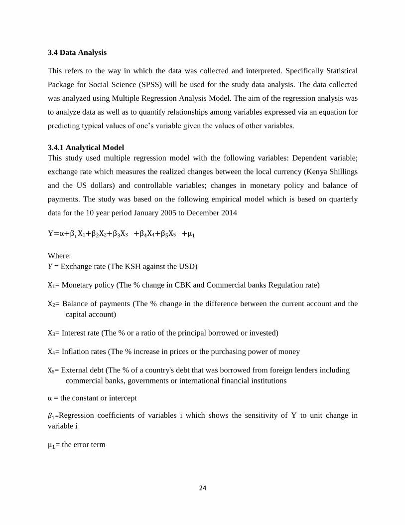
3.4.1 Analytical Model
This study used multiple regression model with the following variables: Dependent variable;
exchange rate which measures the realized changes between the local currency (Kenya Shillings
and the US dollars) and controllable variables; changes in monetary policy and balance of
payments. The study was based on the following empirical model which is based on quarterly
data for the 10 year period January 2005 to December 2014
Y
Where:
Y = Exchange rate (The KSH against the USD)
= Monetary policy (The % change in CBK and Commercial banks Regulation rate)
= Balance of payments (The % change in the difference between the current account and the
capital account)
= Interest rate (The % or a ratio of the principal borrowed or invested)
= Inflation rates (The % increase in prices or the purchasing power of money
= External debt (The % of a country's debt that was borrowed from foreign lenders including
commercial banks, governments or international financial institutions
= the constant or intercept
=Regression coefficients of variables i which shows the sensitivity of Y to unit change in
variable i
= the error term

25
3.4.2 Test of Significance
Data was entered into Statistical Package for Social Sciences (SPSS) version 21 and Microsoft
Office Excel and analyzed using descriptive analysis such as percentage mean and Standard
deviation, correlation and regression analyses. The correlation coefficients from the regression
showed the effect (whether positive or negative) of the independent variables on the dependent
variable. t –test was used to show the significance of the relationship between the controllable
variables and exchange rate. Significance of the relationships was tested at 95% confidence
level. Other statistical tools such as F test for joint significance of all coefficients and R-squared
for the explanatory power of the model were used.

26
CHAPTER FOUR
DATA ANALYSIS, RESULTS AND INTERPRETATION
4.1 Introduction
The broad objective of the study was to examine the effect of changes in monetary policy and
balance of payment on exchange rate in Kenya. The chapter presents findings of the study on
the basis of both descriptive and inferential statistics. The details of descriptive analysis using
frequency distribution tables, descriptive statistics using means and t-tests was used for ranking
the variables under investigation.
4.2 Descriptive statistics
Descriptive measures involved mean, standard deviation and standard error of estimate. The
variables aggregate score was computed as the simple average of the mean scores of the ten
years period. Mean is a measure of central tendency used to describe the most typical value in a
set of values. In addition, standard error of mean (SE) was computed. Standard error of mean is
a measure of reliability of the study results. Standard deviation shows how far the distribution is
from the mean. The results of the descriptive statistics of the variables under study for a period
of ten years (2005-2014) are as indicated in table 4.1
27
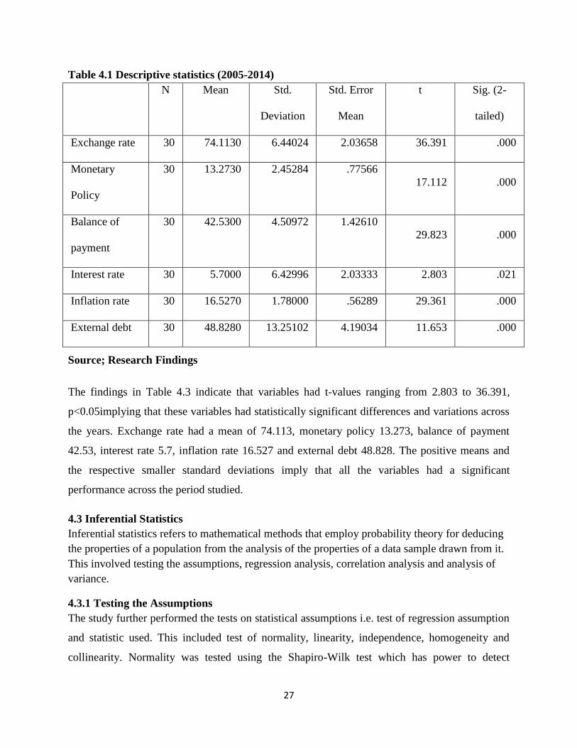
Table 4.1 Descriptive statistics (2005-2014)
N Mean Std.
Deviation
Std. Error
Mean
t Sig. (2-
tailed)
Exchange rate 30 74.1130 6.44024 2.03658 36.391 .000
Monetary
Policy
30 13.2730 2.45284 .77566
17.112 .000
Balance of
payment
30 42.5300 4.50972 1.42610
29.823 .000
Interest rate 30 5.7000 6.42996 2.03333 2.803 .021
Inflation rate 30 16.5270 1.78000 .56289 29.361 .000
External debt 30 48.8280 13.25102 4.19034 11.653 .000
Source; Research Findings
The findings in Table 4.3 indicate that variables had t-values ranging from 2.803 to 36.391,
p<0.05implying that these variables had statistically significant differences and variations across
the years. Exchange rate had a mean of 74.113, monetary policy 13.273, balance of payment
42.53, interest rate 5.7, inflation rate 16.527 and external debt 48.828. The positive means and
the respective smaller standard deviations imply that all the variables had a significant
performance across the period studied.
4.3 Inferential Statistics
Inferential statistics refers to mathematical methods that employ probability theory for deducing
the properties of a population from the analysis of the properties of a data sample drawn from it.
This involved testing the assumptions, regression analysis, correlation analysis and analysis of
variance.
4.3.1 Testing the Assumptions
The study further performed the tests on statistical assumptions i.e. test of regression assumption
and statistic used. This included test of normality, linearity, independence, homogeneity and
collinearity. Normality was tested using the Shapiro-Wilk test which has power to detect

28
departure from normality due to either skewness or kurtosis or both. Its statistic ranges from zero
to one and figures higher than 0.05 indicate the data is normal (Razali and Wah, 2011). Linearity
was tested by use of ANOVA test of linearity which computes both the linear and nonlinear
components of a pair of variables whereby nonlinearity is significant if the F significance value
for the nonlinear component is below 0.05 (Zhang et al., 2011). Independence of error terms,
which implies that observations are independent, was assessed through the Durbin-Watson test
whose statistic ranges from zero to four. Scores between 1.5 and 2.5 indicate independent
observations (Garson, 2012).
Homoscedasticity was tested by use of Levene‘s test of homogeneity of variances. If the Levene
statistic is significant at = 0.05 then the data groups lack equal variances (Gastwirth et al.,
2009). Levene‘s test measures whether or not the variance between the dependent and
independent variables is the same. Thus it is a check of whether the spread of the scores
(reflected in the variance) in the variables are approximately similar (Bryk andRaudenbush,
1988). Multicollinearity was tested by computing the Variance Inflation Factors (VIF) and its
reciprocal, the tolerance. It is a situation in which the predictor variables in a multiple regression
analysis are themselves highly correlated making it difficult to determine the actual contribution
of respective predictors to the variance in the dependent variable. The multicollinearity
assumption has a VIF threshold value of 10 maximum (Robinson and Schumacker, 2009).
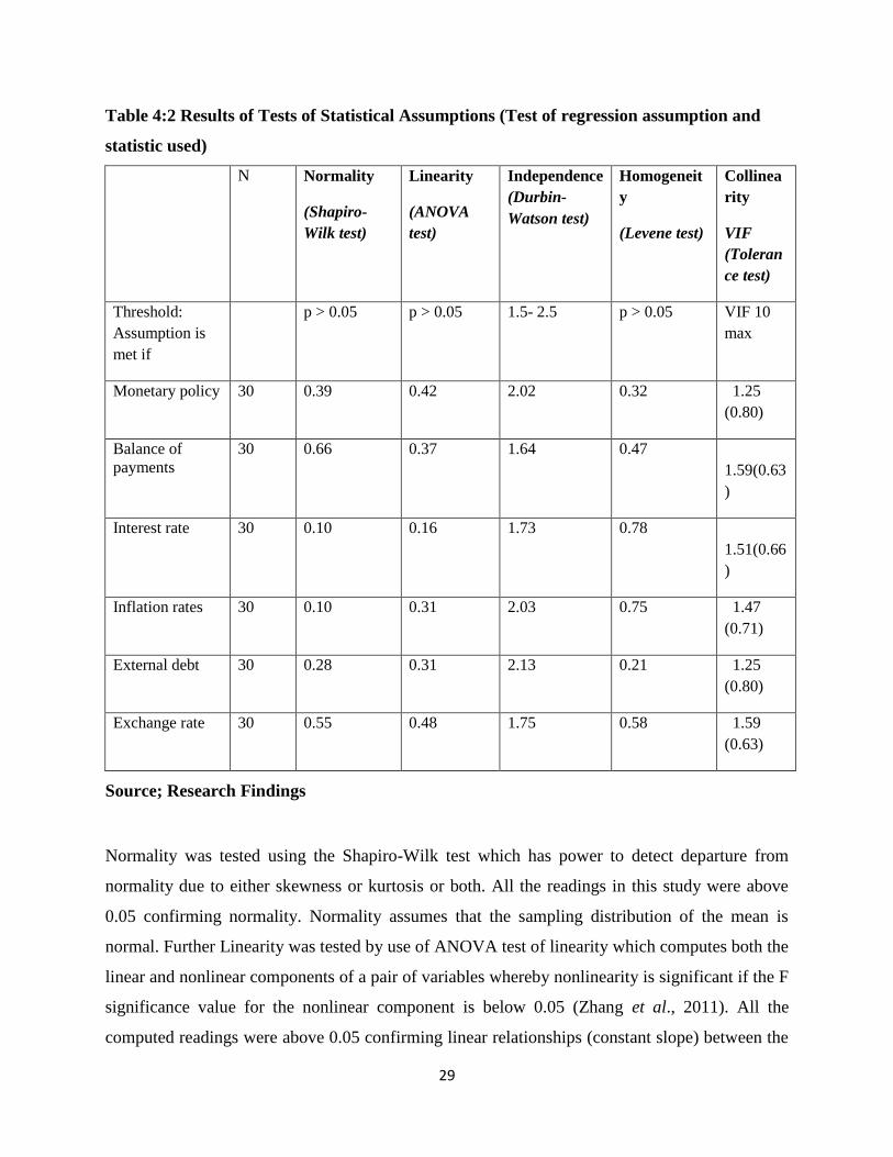
Five assumptions of regression were tested and their results together with those of the test for
reliability are summarized in Table 4.2. The threshold levels for the respective test statistics are
listed below each assumption. For multicollinearity both the variance inflation factor (VIF) and
its reciprocal (Tolerance) values are listed, the latter in parentheses. The results showed that the
assumptions of regression were met and subsequently the data were subjected to further
statistical analysis including correlation and regression as discussed in the following subsections.
29
Table 4:2 Results of Tests of Statistical Assumptions (Test of regression assumption and
statistic used)
N Normality
(Shapiro-
Wilk test)
Linearity
(ANOVA
test)
Independence
(Durbin-
Watson test)
Homogeneit
y
(Levene test)
Collinea
rity
VIF
(Toleran
ce test)
Threshold:
Assumption is
met if
p > 0.05 p > 0.05 1.5- 2.5 p > 0.05 VIF 10
max
Monetary policy 30 0.39 0.42 2.02 0.32 1.25
(0.80)
Balance of
payments
30 0.66 0.37 1.64 0.47
1.59(0.63
)
Interest rate 30 0.10 0.16 1.73 0.78
1.51(0.66
)
Inflation rates 30 0.10 0.31 2.03 0.75 1.47
(0.71)
External debt 30 0.28 0.31 2.13 0.21 1.25
(0.80)
Exchange rate 30 0.55 0.48 1.75 0.58 1.59
(0.63)
Source; Research Findings
Normality was tested using the Shapiro-Wilk test which has power to detect departure from
normality due to either skewness or kurtosis or both. All the readings in this study were above
0.05 confirming normality. Normality assumes that the sampling distribution of the mean is
normal. Further Linearity was tested by use of ANOVA test of linearity which computes both the
linear and nonlinear components of a pair of variables whereby nonlinearity is significant if the F
significance value for the nonlinear component is below 0.05 (Zhang et al., 2011). All the
computed readings were above 0.05 confirming linear relationships (constant slope) between the
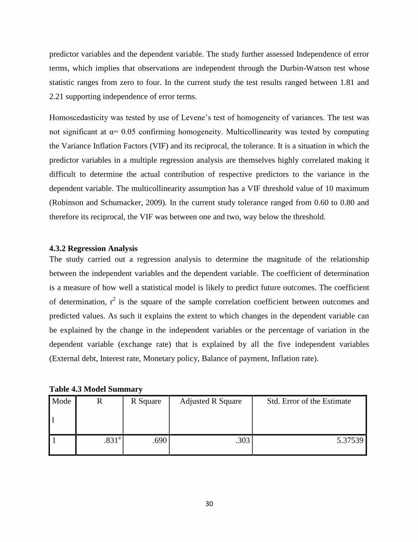
30
predictor variables and the dependent variable. The study further assessed Independence of error
terms, which implies that observations are independent through the Durbin-Watson test whose
statistic ranges from zero to four. In the current study the test results ranged between 1.81 and
2.21 supporting independence of error terms.
Homoscedasticity was tested by use of Levene‘s test of homogeneity of variances. The test was
not significant at = 0.05 confirming homogeneity. Multicollinearity was tested by computing
the Variance Inflation Factors (VIF) and its reciprocal, the tolerance. It is a situation in which the
predictor variables in a multiple regression analysis are themselves highly correlated making it
difficult to determine the actual contribution of respective predictors to the variance in the
dependent variable. The multicollinearity assumption has a VIF threshold value of 10 maximum
(Robinson and Schumacker, 2009). In the current study tolerance ranged from 0.60 to 0.80 and
therefore its reciprocal, the VIF was between one and two, way below the threshold.
4.3.2 Regression Analysis
The study carried out a regression analysis to determine the magnitude of the relationship
between the independent variables and the dependent variable. The coefficient of determination
is a measure of how well a statistical model is likely to predict future outcomes. The coefficient
of determination, r2 is the square of the sample correlation coefficient between outcomes and
predicted values. As such it explains the extent to which changes in the dependent variable can
be explained by the change in the independent variables or the percentage of variation in the
dependent variable (exchange rate) that is explained by all the five independent variables
(External debt, Interest rate, Monetary policy, Balance of payment, Inflation rate).
Table 4.3 Model Summary
Mode
l
R R Square Adjusted R Square Std. Error of the Estimate
1 .831a .690 .303 5.37539
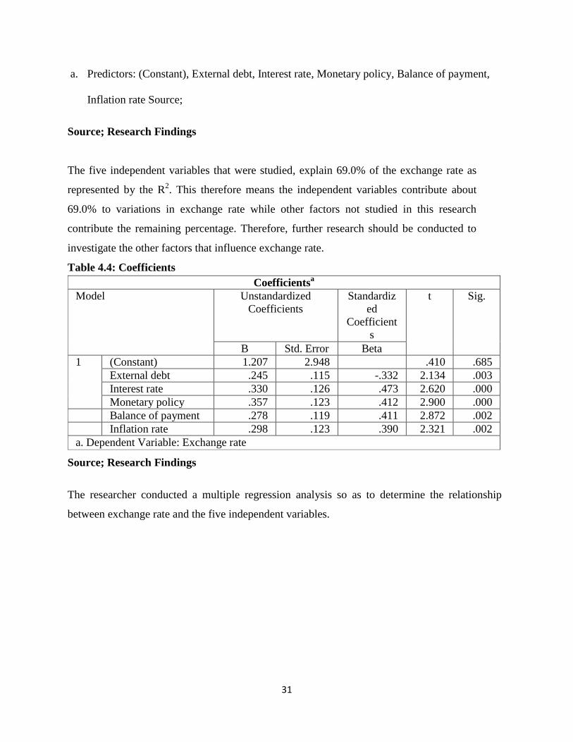
31
a. Predictors: (Constant), External debt, Interest rate, Monetary policy, Balance of payment,
Inflation rate Source;
Source; Research Findings
The five independent variables that were studied, explain 69.0% of the exchange rate as
represented by the R2. This therefore means the independent variables contribute about
69.0% to variations in exchange rate while other factors not studied in this research
contribute the remaining percentage. Therefore, further research should be conducted to
investigate the other factors that influence exchange rate.
Table 4.4: Coefficients
Coefficientsa
Model Unstandardized
Coefficients
Standardiz
ed
Coefficient
s
t Sig.
B Std. Error Beta
1 (Constant) 1.207 2.948 .410 .685
External debt .245 .115 -.332 2.134 .003
Interest rate .330 .126 .473 2.620 .000
Monetary policy .357 .123 .412 2.900 .000
Balance of payment .278 .119 .411 2.872 .002
Inflation rate .298 .123 .390 2.321 .002
a. Dependent Variable: Exchange rate
Source; Research Findings
The researcher conducted a multiple regression analysis so as to determine the relationship
between exchange rate and the five independent variables.

32
The regression equation (Y =0+ β1X1+β2 X2+β3 X3+β4 X4+β5 X5) now becomes:
Y = 1.207 +0.245 X1 +0.330X2 + 0.357X3+
0.278X4+ 0.298X5
The multiple linear regression models indicate that all the independent variables have positive
coefficient. The regression results above reveal that there is a positive relationship between
dependent variable (exchange rate) and independent variables (External debt, Interest rate,
Monetary policy, Balance of payment, Inflation rate). The t statistics helps in determining the
relative importance of each variable in the model. As a guide regarding useful predictors, we
look for t values well below -0.5 or above +0.5.
4.3.3 Correlation Analysis
The study conducted Pearson‘s correlation coefficient. The Pearson product-moment correlation
coefficient (or Pearson correlation coefficient for short) is a measure of the strength of a linear
association between two variables and is denoted by r. The Pearson correlation coefficient, r, can
take a range of values from +1 to -1. A value of 0 indicates that there is no association between
the two variables. A value greater than 0 indicates a positive association, that is, as the value of
one variable increases so does the value of the other variable. A value less than 0 indicates a
negative association, that is, as the value of one variable increases the value of the other variable
decreases.

33
Table 4.5 Correlation Results
Source; Research Findings
Monetary
policy
Balance
of
payment
Interest
rate
Inflation
rate
Externa
l debt
Exchange
rate
Monetar
y policy
Pearson
Correlation
Sig. (2- tailed)
N
1
0.000
30
Balance
of
payment
Pearson
Correlation
Sig. (2- tailed)
N
0.742
0.000
30
1
0.000
30
Interest
rate
Pearson
Correlation
Sig. (2- tailed)
N
0.842
0.000
30
0.542
0.000
30
1
0.000
30
Inflation
rate
Pearson
Correlation
Sig. (2- tailed)
N
0.771
0.000
30
0.664
0.000
30
0.732
0.000
30
1
0.000
30
External
debt
Pearson
Correlation
Sig. (2- tailed)
N
0.421
0.047
30
0.342
0.038
30
0.341
0.037
30
0.232
0.413
30
1
0.000
30
Exchang
e rate
Pearson
Correlation
Sig. (2- tailed)
N
0.811
0.000
30
0.532
0.000
30
0.691
0.000
30
0.789
0.000
30
0.352
0.170
30
1
0.000
30
** Correlation is significant at the 0.01 level (2-tailed).
* Correlation is significant at the 0.05 level (2-tailed).

34
The results in Table 4.5 indicate that the relationship between monetary policy and Exchange
rate is strong, positive and statistically significant (r=.811, p-value=.000). Similarly, the
relationship between inflation rate and Exchange rate is strong, positive and statistically
significant (r=.789, p-value=.000). The relationship between interest rate and balance of payment
was also significant and strong (r=.691, p-value=.000) and (r=.532, p-value=.000) respectively.
However the relationship between external debt and exchange rate is positive but insignificant as
indicated by Pearson correlation coefficient of .352 and p-value=.000. This implies that
monetary policy, balance of payment, interest rate, inflation rate and external debt play a critical
role of influencing Exchange rate in Kenya. The strongest relationship was between monetary
policy and Exchange rate (r=.811, p-value=.000).
4.3.4 Analysis of Variance (ANOVA)
The statistical F test is used to determine how well the regression equation fits the data. In this
study, the F value of 7.786 was significant at the 1% level, indicating that at least one of the
independent variables helped to explain some of the variation in exchange rate.
Table 4.6: Analysis of Variance
ANOVAa
Model Sum of Squares df Mean
Square
F Sig.
1
Regression 272.606 4 68.151 7.786 .000b
Residual 323.870 37 8.753
Total 596.476 41
a. Dependent Variable: Exchange rate
b. Predictors: (Constant), External debt, Interest rate, Monetary policy, Balance of
payment, Inflation rate
Source; Research Findings
4.4 Interpretation of the Findings
The results presented focused on the effects of external debt, interest rate, monetary policy,
balance of payment and inflation rate on exchange rate in Kenya. The broad objective of the
study was to examine the effect of changes in monetary policy and balance of payment on
35
exchange rate in Kenya. Descriptive statistics was first performed which involved mean,
standard deviation and standard error of estimate. The variables aggregate score was computed
as the simple average of the mean scores of the ten years period. The findings indicated that
variables had high t-values implying that these variables had statistically significant differences
and variations across the years. The positive means and the respective smaller standard
deviations imply that all the variables had a significant performance across the period studied.
The study conducted Pearson‘s correlation coefficient which is a measure of the strength of a
linear association between two variables and is denoted by r. The results indicated that the
relationship between monetary policy and Exchange rate is strong, positive and statistically
significant. Similarly, the relationship between inflation rate and Exchange rate is strong,
positive and statistically significant. The relationship between interest rate and balance of
payment was also significant and strong and respectively. However the relationship between
external debt and exchange rate is positive but insignificant. This implies that monetary policy,
balance of payment, interest rate, inflation rate and external debt play a critical role of
influencing Exchange rate in Kenya. The strongest relationship was between monetary policy
and Exchange rate.
The study further carried out a regression analysis to determine the magnitude of the relationship
between the independent variables and the dependent variable. The five independent variables
that were studied, explained 69.0% of the exchange rate as represented by the R2. The multiple
linear regression models indicated that all the independent variables had positive coefficient. The
regression results revealed that there is a positive relationship between dependent variable
(exchange rate) and independent variables (External debt, Interest rate, Monetary policy, Balance
of payment, Inflation rate). The study is hence consistent with other previous studies.

36
CHAPTER FIVE
SUMMARY, CONCLUSION AND RECOMMENDATIONS
5.1 Introduction
This chapter summarizes the study and makes conclusion based on the results. The implications
from the findings and areas for further research are also presented. This section presents the
findings from the study in comparison to what other scholars have said as noted under literature
review.
5.2 Summary
The results presented focused on the effects of External debt, Interest rate, Monetary policy,
Balance of payment and Inflation rate on exchange rate in Kenya. This section lays emphasis on
the summary of the findings. The results from the statistical tests are compared with other
empirical and theoretical propositions and both areas of agreement or disagreement with such
propositions are summarized.
Multiple regressions were carried out at 95.0 percent confidence level to test the relationships
and the statistical significance of the study variables. The same was applied to the other variables
to determine their effects. The independent effects were first analyzed using correlation analysis
followed by combined analysis through regression analysis. Multiple linear regressions analysis
was applied on the relative correlations on strength of the relationship between the variables
whether strong or weak. The R2
values showed the proportion of the variation indicator that
accounted for by the combined effects in the model. F-values indicated the significance of the
model on performance at 95% confidence level.
The broad objective of the study was to examine the effect of changes in monetary policy and
balance of payment on exchange rate in Kenya. First various assumptions were made about
variables during statistical tests. This was to ensure that the findings were worth using in
decision making. Failure to meet these assumptions may havelead to Type I or Type II errors.
Testing for assumptions is beneficial because it ensures that analysis meets associated

37
assumptions and helps avoid Type I and Type II errors (Osborne et al, 2001). This study carried
out test of normality and multicollinearity tests.
In this study the normality was tested using Kolmogorov-Smirnov Test and the Shapiro-Wilk
Test. Shapiro-Wilk Test is more appropriate for small sample sizes (< 50 samples) like this
study. It is a more reliable test for determining skewness and kurtosis values of normality. If it is
below 0.05, the data significantly deviate from a normal distribution. The results of the tests of
normality on the variables showed that all the p-values were greater than the alpha level of
(0.05). Shapiro-Wilk Test results were (0.428, 0.219, 0.322, .413, .376) greater than 0.05
confirming the data was normal.
The test for Multicollinearity was conducted to assess whether one or more of the variables of
interest is highly correlated with one or more of the other independent variables. The variance
inflation factor (VIF) was used to evaluate the level of correlation between variables and to
estimate how much the variance of a coefficient was inflated because of linear dependence with
other predictors. As a rule of thumb if any of the VIF are greater than 10 (greater than 5 when
conservative) then there is a probability of a problem with Multicollinearity and is harmful to the
study. The results revealed that there was no serious problem with multicollinearity. The
variance inflation factors for the variables were all below 5 meaning that the variables were not
highly correlated.
Descriptive measures involved mean, standard deviation and standard error of estimate. The
variables aggregate score was computed as the simple average of the mean scores of the ten
years period. The findings indicated that variables had high t-values implying that these variables
had statistically significant differences and variations across the years. The positive means and
the respective smaller standard deviations imply that all the variables had a significant
performance across the period studied.
The study conducted Pearson‘s correlation coefficient. The Pearson product-moment correlation
coefficient (or Pearson correlation coefficient for short) is a measure of the strength of a linear
association between two variables and is denoted by r. The results indicated that the relationship
between monetary policy and Exchange rate is strong, positive and statistically significant.
Similarly, the relationship between inflation rate and Exchange rate is strong, positive and

38
statistically significant. The relationship between interest rate and balance of payment was also
significant and strong and respectively. However the relationship between external debt and
exchange rate is positive but insignificant. This implies that monetary policy, balance of
payment, interest rate, inflation rate and external debt play a critical role of influencing Exchange
rate in Kenya. The strongest relationship was between monetary policy and Exchange rate.
The study further carried out a regression analysis to determine the magnitude of the relationship
between the independent variables and the dependent variable. The five independent variables
that were studied, explain 69.0% of the exchange rate as represented by the R2. The multiple
linear regression models indicate that all the independent variables have positive coefficient. The
regression results above reveal that there is a positive relationship between dependent variable
(exchange rate) and independent variables (External debt, Interest rate, Monetary policy, Balance
of payment, Inflation rate).
5.3 Conclusion
The analysis of the correlations results seemed to support the argument that each independent
variable has its own particular informative value in the ability to explain exchange rate. The
significance of the coefficients was calculated at the level of 95%. The study findings indicate
that external debt, interest rate, monetary policy, balance of payment and inflation rate are
statistically significant to exchange rate as indicated by the positive and strong Pearson
correlation coefficients.
According to the regression equation established, taking all factors into account (external debt,
interest rate, monetary policy, balance of payment and inflation rate), exchange rate will be
1.207. A Pearson coefficient measure showed a strong, significant, positive relationship between
the predictor variables on exchange rate in Kenya. The findings showed that predictor variables
considered in the model are significantly associated with exchange rate as indicated by the
positive mean values and their respective standard deviations.
39
5.4 Policy Recommendations
Based on the research findings, the study recommends that balance of payments and monetary
policies should be controlled appropriately by the policy makers so as to maintain exchange rate
at a harmless point to the overall economy. The study further recommends that other
determinants of exchange rate such as inflation and interest rate as significantly indicated in the
study should be regularly checked and corrected to avoid a paradigm shift in the exchange rate
which may negatively impact the economy. The government should also set up monetary
policies on exchange rates so as to keep it friendly to the overall economy.
5.5 Limitations of the Study
Although this study helped to shed light on the dynamics of monetary policy and balance of
payment on exchange rate in Kenya, it was subject to a number of limitations. These mainly
related to the setup of the study relative to the resources available within the research period. As
such the constraints influenced the scale of the study but did not affect the conduct of the
research once the design was arrived at.
Since the main purpose of this study is to identify the relationship between monetary policy and
balance of payment on exchange rate in Kenya, central bank considered some information
sensitive and confidential and thus the researcher had to convince them that the purpose of
information is for academic research only and may not be used for any other intentions.
Monetary policy and balance of payment keep on changing from period to period depending on
prevailing economic situations and demand on the capital market. The findings therefore may not
reflect the true effect of such variables on exchange rate across a period of 10 years since some
measures keeps fluctuating.
5.6 Suggestions for Further Research
This study used only five variables to test their influence on exchange rate in Kenya. Given the
fact that there are many other factors that may affect exchange rate, other researchers may seek
to unravel the influence of such other factors like political influence, fiscal policies and so forth
on the exchange rate. It would be interesting to find out whether the results would be the same
when different variables are used. Given the critical role that monetary policies play in the
monetary economy, it would also be interesting for future research to study the influence of

40
monetary policy as an independent variable and exchange rate as a dependent variable. With
only secondary data, triangulating the data is complex. Future research should consider
combining both secondary and primary data.

41
REFERENCES
Bergen, J. V. (2010). Factors That Influence Exchange Rates,. Investopedia,
http://www.investopedia.com/articles/basics/04/050704.asp#axzz288SmcagR .
Bryman, A., & Bell, E. (2007). Business Research Methods. Oxford University Press.
Diffu, I. (2011). The Relationship between Foreign Exchange Risk and Financial Performance
of Airlines in Kenya: A Case Study of Kenya Airways. Unpublished MBA Project,
University of Nairobi .
Calvo, G. A., & Reinhart, C. M. (2002). Fear of Floating. Quarterly Journal of Economics, 117
(2) , 379-408.
Chou, W. (2000). Exchange Rate Variability and China‘s Exports. Journal of Comparative
Economics (28), 61-79.
Cooper, & Schindler. (2008). Business Research Methods. New York : McGraw Hill Irwin.
Dornbusch, R. (1974) The Renminbi Exchange Rate Revaluation: Theory, Practice, and Lessons
from Japan. ADBI Policy Papers; no. 9.
Dornbusch, R., & Fisher, S. (1980). International Financial Crisis. CESifo Working Paper, 926.
Edwards, S., & Ahamed, L. (2012). Economic adjustment and exchange rates in developing
countries. Chicago: University of Chicago Press.
Frenkel, J. A., & Levich, R. M. (1975). Covered Interest Arbitrage: Unexploited Profits?
Journal of Political Economy 83 , 325-338.
Frankel, J. A. (2008). On exchange rates. Cambridge, Mass: MIT Press.
Gbosi, F. J. (2002). Commercial Bank Financial Management. Prentice Hall International, Inc.
Gerrard, C. D., & Lucas, R. F. (2013). Monetary policy in developing countries: lessons from
Kenya. Journal of International Trade & Economic Development , 12 (2).
Hornsby, C. (2012). Kenya: a history since independence. London: I. B. Tauris.
IMF. (2011 ). Kenya. Washington DC: International Monetary Fund.
IMF. (2007). The Impact of Monetary Policy on the Bilateral Exchange Rate. Washington,
D.C: International Monetary Fund.
IMF. (2010). The monetary approach to the balance of payments. Washington, DC:
International Monetary Fund.

42
James, J., & Marsh, I. W. (2012). Handbook of exchange rates. Hoboken: John Wiley & Sons,
Inc.
Kafka, A. (2008). THE NEW EXCHANGE RATE REGIME AND THE DEVELOPING
COUNTRIES. . Journal of Finance , Vol. 33 Issue 3, p795-802.
Kamau, A. W., & Sichei, M. M. (2013). Demand for Money: Implications for the Conduct of
Monetary Policy in Kenya. International Journal of Economics & Finance , Vol. 4
Issue 8, p72-82.
Kandil, A. (2007). Estimating renminbi (RMB) equilibrium exchange rate, Journal of Policy Modelling,
29 (3), 417-29.
Kasekende, L., & Brownbridge, M. (2011). Post-crisis Monetary Policy Frameworks in sub-
Saharan Africa. . African Development Review , Vol. 23 Issue 2, p190-201.
Kennedy, O. (2013). Kenya's foreign trade balance: an empirical investigation. European
Scientific Journal , Vol. 9 Issue 19, p176.
Khan, J. A. (2011). Research methodology. New Delhi: APH Publishing Corporation.
Kimani, N. (2013). International trade policies. Washington, DC: Internat. Monetary Fund.
Kisinguh, K. N., & Kamau, A. W. (2013). An Empirical Investigation of Exchange Rate
Determination in Kenya. Advances in Management & Applied Economics , Vol. 3
Issue 2, p165-178.
KNBS. (2009). Economic survey. Nairobi: Kenya National Bureau of Statistics .
Kothari, C. R. (2005). Research methodology: methods & techniques. New Delhi: New Age
International.
Kumar, R. (2010). Research Methodology. London: SAGE.
Matheson, L., & Lacey, F. M. (2011). Doing Your Literature Review. London: SAGE.
Marsha, R. S. (1994). Impact of Exchange Rate Volatility on Indonesia‘s Trade Performance in
the 1990s. The Japanese and International Economies, 18 , 218-240.
McKenzie, M. D. (1998). The Impact of Exchange Rate Volatility on Australian Trade Flows .
Journal of International Financial Markets, Institutions and Money, 8, 21-38.
Miller, N. C. (2009). Balance of payments and exchange rate theories. Cheltenham: Edward
Elgar Publishing.
Misati, R. N. (2012). Asset prices and monetary policy in Kenya. Journal of Economic
Studies , 39 (4), 451-468.

43
Mishkin, F. S. (2007). Monetary policy strategy. Cambridge, Mass: MIT Press.
Mouyad, A. S. (2009). The Determinants of Real Exchange Rate Volatility in the Syrian
Economy. Centre d'Économie de la Sorbonne - Université Paris-1-Panthéon-Sorbonne .
Mugenda, O. M., & Mugenda, A. G. (1999). Research Methods: Quantitative and Qualitative
Approaches. African Centre for Technology Studies.
Musyoki, D. (2012). Real Exchange Rate Equilibrium And Misalignment In Kenya. Journal
of Business Studies Quarterly , 3 (4), 24-42.
Ndung'u, N. S. (2012). The Exchange Rate and Monetary Policy in Kenya. African
Development Review , 12 (1), 24.
Ngerebo, T. A. (2012). The Impact of Foreign Exchange Fluctuation on the Intermediation of
Banks in Nigeria (1970 – 2004). African Journal of Business Management , 6 (11), 3872-
3879.
Nnanna, K. (2001). Exchange Rate Dynamics Redux. The Journal of Political Economy , 103
(3), 624-660.
Ochieng', W. R., & Maxon, R. M. (2002). An economic history of Kenya. Nairobi, Kenya:
East African Educational Publishers.
Okiogo, C. K. (2013). The upshot of financial Sector regulation on the financial market
performance in Kenya Perspectives. Business Management Dynamics , 2 (9), 1-14.
Okoth, A. (2006). African nationalism and the de-colonisation process. Nairobi: East African
Educational Publ.
Onyancha, C. K. (2011). The Impact of Exchange Rate Movements on the Financial
Performance of International Non Governmental Organizations. Unpublished MBA
Project, University of Nairobi .
Otuori, O. H. (2013). Influence of exchange rate determinants on the performance of
commercial banks in Kenya. , . European Journal of Management Sciences and
Economics, 1 (2), 86-98.
Rabin, J. (2010). Balance of Payments Manual. Washington DC: International Monetary
Fund.
Rwabutoga, G. R. (2005). Comprehensive Commerce. Nairobi: East African Publishers.
Were, M. (2014). Assessing the effectiveness of monetary policy in Kenya: Evidence from a
macroeconomic model. Research Department, Central Bank of Kenya , 37:193-201.

44
Santoso, S. (2011), Transmissions of real economic shocks across the Pacific Rim economies", Journal of
Policy Modelling, 26 (8-9), 959-72.
Solnik, B. (2000). International Investments (4 ed.). Addison-Wesley Copyright Addison
Wesley Longman.
Stavarek, B. C. (2004). Post-Martem of Financial Performance and Prediction of Future Earning
Capability of a Bank: An Application of CAMEL Rating and Balanced Scorecard. Indian
Journal of Accounting, 34 (1), 8-16.
Suranovic, R. (2010). Exchange Rate Volatility, Trade and ‗Fixing for Life‘ in Thailand. Japan
and the World Economy (14), 445-470.
Tailor, C. (2004). Credit Reporting, Relationship Banking, and Loan Repayment. Swiss
National Bank Working Papers 2006-03 .
Zettelmeyer, J. (2009). The Impact of Monetary Policy on the Exchange Rate. Washington
DC: International Monetary Fund.

45
APPENDICES
APPENDIX I: Raw Data
Year Exchange Rate
Monetary policy
Balance of payments
Interest rate
Inflation rate
External Debt
2005
1 68.55 8.07 38.95 8.00 14.54 35.78
2 65.53 8.93 34.71 9.00 15.91 43.56
3 66.23 9.44 36.31 9.00 14.01 36.45
2006
1 62.70 7.21 37.02 2.00 14.46 51.23
2 67.70 7.59 34.85 15.00 14.19 52.21
3 65.45 9.32 35.22 3.00 13.98 53.34
2007 37.61 8.00 14.83
1 66.35 9.39 35.93 8.00 13.03 53.23
2 73.85 10.47 36.74 -5.00 17.55 49.45
3 79.30 13.04 39.89 22.00 16.33 50.34
2008
1 89.95 9.00 40.11 6.00 15.18 67.56
2 87.60 10.31 41.01 4.00 14.54 68.23
3 83.05 12.89 41.04 1.00 14.90 69.23
2009
1 79.65 12.12 41.14 9.00 16.32 70.23
2 78.60 12.36 42.44 7.00 16.29 67.45
3 78.85 13.37 43.11 8.00 16.18 69.47
2010
1 75.55 14.43 43.39 4.00 19.98 59.56
2 78.55 14.88 44.37 2.00 19.67 54.65
3 75.20 12.60 43.94 1.00 17.20 53.98
2011
1 78.50 12.69 43.73 4.00 17.47 49.43
2 73.60 13.18 42.13 7.00 19.47 46.70
3 74.05 15.48 43.36 6.00 18.07 45.23
2012
1 79.80 13.97 45.97 5.00 19.44 46.45
2 68.70 14.50 45.10 4.00 19.17 45.34
3 69.65 14.12 45.91 1.00 17.21 43.45
2013
1 65.55 16.93 47.43 0.00 17.32 24.54
2 67.70 15.58 47.81 3.00 18.22 30.23

46
3 68.15 16.11 49.16 4.00 18.39 30.45
2014
1 78.30 15.30 46.15 0.00 19.04 32.45
2 78.60 15.21 40.97 3.00 19.60 33.34
3 81.20 16.36 47.36 2.00 19.00 36.34
Source: Research findings

47
APPENDIX II: Output
Tests of Normality
Kolmogorov-Smirnova Shapiro-Wilk
Statistic df Sig. Statistic df Sig.
Monetary policy .072 29 .200* .979 29 .428
Balance of payments .093 29 .200* .972 29 .219
Interest rate .085 29 .200* .976 29 .322
Inflation rate .077 29 .200* .979 29 .413
External debt .841 29 .200* .979 29 .376
Test for Multicollinearity
Model Collinearity Statistics
Tolerance VIF
Monetary policy 772 1.295
Balance of payments 698 1.433
Interest rate 873 1.146
Inflation rate 756 1.321
External debt 812 1.154
Descriptive statistics
N Mean Std.
Deviation
Std. Error
Mean
t Sig. (2-
tailed)
Exchange rate 30 74.1130 6.44024 2.03658 36.391 .000
Monetary
policy
30 13.2730 2.45284 .77566 17.112 .000

48
Balance of
payment
30 42.5300 4.50972 1.42610 29.823 .000
Interest rate 30 5.7000 6.42996 2.03333 2.803 .021
Inflation rate 30 16.5270 1.78000 .56289 29.361 .000
External debt 30 48.8280 13.25102 4.19034 11.653 .000
Inferential Analysis
Correlation Results
Monetary
policy
Balance
of
payment
Interest
rate
Inflation
rate
Externa
l debt
Exchange
rate
Monetar
y policy
Pearson
Correlation
Sig. (2- tailed)
N
1
0.000
30
Balance
of
payment
Pearson
Correlation
Sig. (2- tailed)
N
0.742
0.000
30
1
0.000
30
Interest
rate
Pearson
Correlation
Sig. (2- tailed)
N
0.842
0.000
30
0.542
0.000
30
1
0.000
30
Inflation
rate
Pearson
Correlation
Sig. (2- tailed)
N
0.771
0.000
30
0.664
0.000
30
0.732
0.000
30
1
0.000
30
External
debt
Pearson
Correlation
Sig. (2- tailed)
0.421
0.047
0.342
0.038
0.341
0.037
0.232
0.413
1
0.000

49
Model Summary
Mo
del
R R Square Adjusted R Square Std. Error of the Estimate
1 .831a .690 .303 5.37539
b. Predictors: (Constant), External debt, Interest rate, Monetary policy, Balance of
payment, Inflation rate Source;
ANOVAa
Model Sum of Squares df Mean
Square
F Sig.
1 Regressi
on
272.606 4 68.151 7.786 .000b
Residual 323.870 37 8.753
Total 596.476 41
a. Dependent Variable: Exchange rate
b. Predictors: (Constant), External debt, Interest rate, Monetary policy, Balance of
payment, Inflation rate
Coefficientsa
Model Unstandardized
Coefficients
Standardize
d
Coefficient
s
t Sig.
B Std. Error Beta
1 (Constant) 1.207 2.948 .410 .685
External debt .245 .115 -.332 2.134 .003
Interest rate .330 .126 .473 2.620 .000
Monetary policy .357 .123 .412 2.900 .000
Balance of payment .278 .119 .411 2.872 .002
Inflation rate .298 .123 .390 2.321 .002
a. Dependent Variable: Exchange rate
N 30 30 30 30 30
Exchang
e rate
Pearson
Correlation
Sig. (2- tailed)
N
0.811
0.000
30
0.532
0.000
30
0.691
0.000
30
0.789
0.000
30
0.352
0.170
30
1
0.000
30
** Correlation is significant at the 0.01 level (2-tailed).
* Correlation is significant at the 0.05 level (2-tailed).
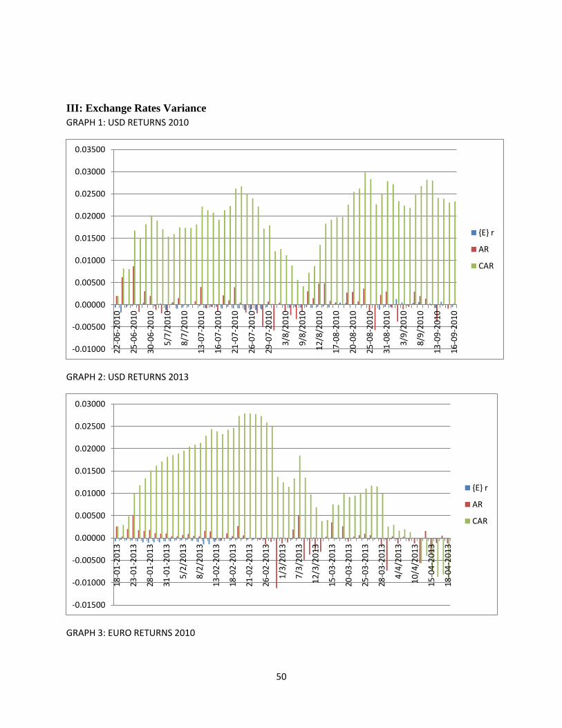
50
III: Exchange Rates Variance
GRAPH 1: USD RETURNS 2010
GRAPH 2: USD RETURNS 2013
GRAPH 3: EURO RETURNS 2010
-0.01000
-0.00500
0.00000
0.00500
0.01000
0.01500
0.02000
0.02500
0.03000
0.03500
22
-06
-20
10
25
-06
-20
10
30
-06
-20
10
5/7
/20
10
8/7
/20
10
13
-07
-20
10
16
-07
-20
10
21
-07
-20
10
26
-07
-20
10
29
-07
-20
10
3/8
/20
10
9/8
/20
10
12
/8/2
01
0
17
-08
-20
10
20
-08
-20
10
25
-08
-20
10
31
-08
-20
10
3/9
/20
10
8/9
/20
10
13
-09
-20
10
16
-09
-20
10
{E} r
AR
CAR
-0.01500
-0.01000
-0.00500
0.00000
0.00500
0.01000
0.01500
0.02000
0.02500
0.03000
18
-01
-20
13
23
-01
-20
13
28
-01
-20
13
31
-01
-20
13
5/2
/20
13
8/2
/20
13
13
-02
-20
13
18
-02
-20
13
21
-02
-20
13
26
-02
-20
13
1/3
/20
13
7/3
/20
13
12
/3/2
01
3
15
-03
-20
13
20
-03
-20
13
25
-03
-20
13
28
-03
-20
13
4/4
/20
13
10
/4/2
01
3
15
-04
-20
13
18
-04
-20
13
{E} r
AR
CAR
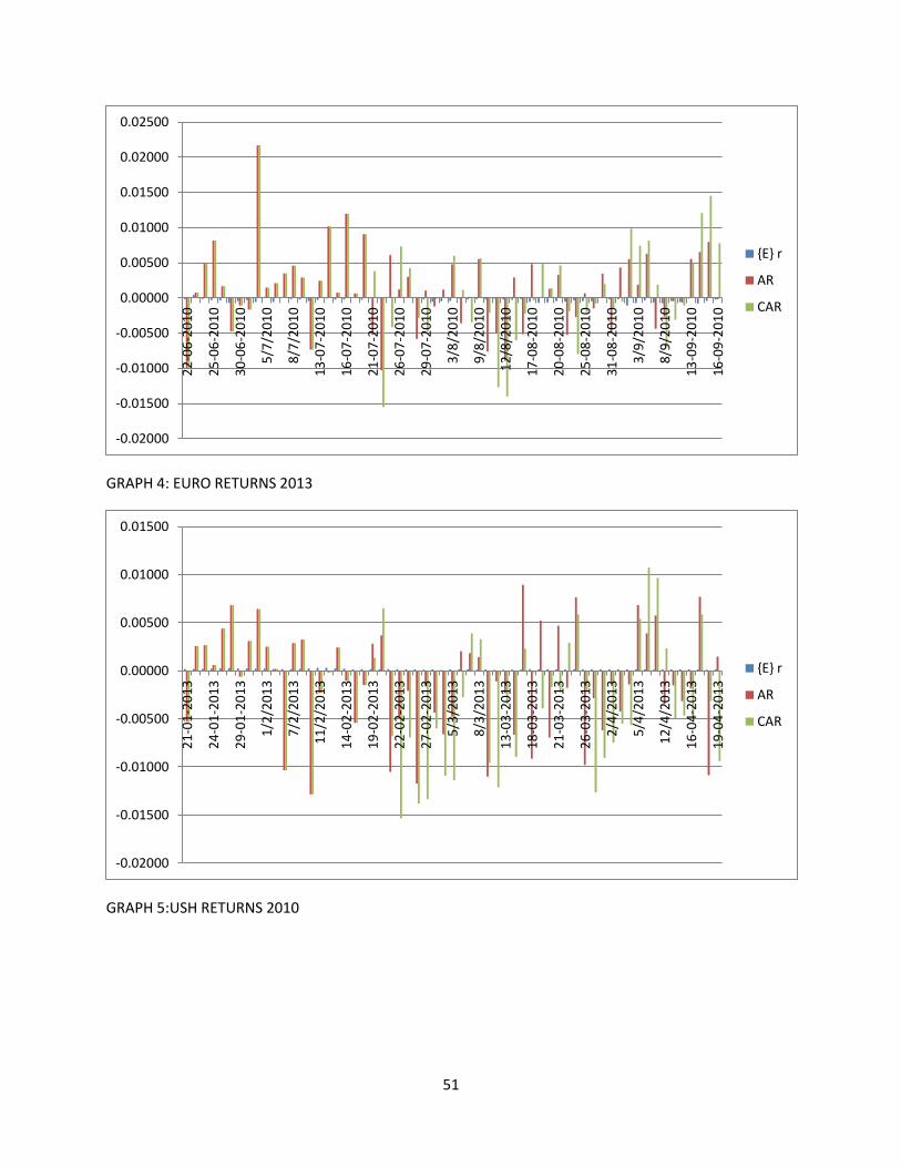
51
GRAPH 4: EURO RETURNS 2013
GRAPH 5:USH RETURNS 2010
-0.02000
-0.01500
-0.01000
-0.00500
0.00000
0.00500
0.01000
0.01500
0.02000
0.02500
22
-06
-20
10
25
-06
-20
10
30
-06
-20
10
5/7
/20
10
8/7
/20
10
13
-07
-20
10
16
-07
-20
10
21
-07
-20
10
26
-07
-20
10
29
-07
-20
10
3/8
/20
10
9/8
/20
10
12
/8/2
01
0
17
-08
-20
10
20
-08
-20
10
25
-08
-20
10
31
-08
-20
10
3/9
/20
10
8/9
/20
10
13
-09
-20
10
16
-09
-20
10
{E} r
AR
CAR
-0.02000
-0.01500
-0.01000
-0.00500
0.00000
0.00500
0.01000
0.01500
21
-01
-20
13
24
-01
-20
13
29
-01
-20
13
1/2
/20
13
7/2
/20
13
11
/2/2
01
3
14
-02
-20
13
19
-02
-20
13
22
-02
-20
13
27
-02
-20
13
5/3
/20
13
8/3
/20
13
13
-03
-20
13
18
-03
-20
13
21
-03
-20
13
26
-03
-20
13
2/4
/20
13
5/4
/20
13
12
/4/2
01
3
16
-04
-20
13
19
-04
-20
13
{E} r
AR
CAR
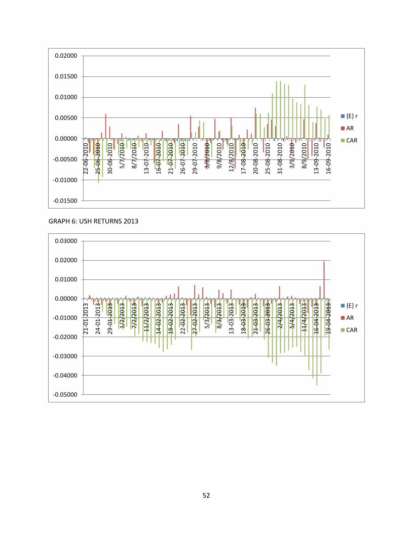
52
GRAPH 6: USH RETURNS 2013
-0.01500
-0.01000
-0.00500
0.00000
0.00500
0.01000
0.01500
0.02000
22
-06
-20
10
25
-06
-20
10
30
-06
-20
10
5/7
/20
10
8/7
/20
10
13
-07
-20
10
16
-07
-20
10
21
-07
-20
10
26
-07
-20
10
29
-07
-20
10
3/8
/20
10
9/8
/20
10
12
/8/2
01
0
17
-08
-20
10
20
-08
-20
10
25
-08
-20
10
31
-08
-20
10
3/9
/20
10
8/9
/20
10
13
-09
-20
10
16
-09
-20
10
{E} r
AR
CAR
-0.05000
-0.04000
-0.03000
-0.02000
-0.01000
0.00000
0.01000
0.02000
0.03000
21
-01
-20
13
24
-01
-20
13
29
-01
-20
13
1/2
/20
13
7/2
/20
13
11
/2/2
01
3
14
-02
-20
13
19
-02
-20
13
22
-02
-20
13
27
-02
-20
13
5/3
/20
13
8/3
/20
13
13
-03
-20
13
18
-03
-20
13
21
-03
-20
13
26
-03
-20
13
2/4
/20
13
5/4
/20
13
11
/4/2
01
3
16
-04
-20
13
19
-04
-20
13 {E} r
AR
CAR