Embed Size (px)
Citation preview

J. Fluid Mech. (1997), vol. 330, pp. 307–338
Copyright c© 1997 Cambridge University Press
307
The effect of compressibility on turbulent shearflow: a rapid-distortion-theory anddirect-numerical-simulation study
By A. S I M O N E1, G. N. C O L E M A N2 AND C. C A M B O N1
1Ecole Centrale de Lyon, Laboratoire de Mecanique des Fluides et d’Acoustique,UMR CNRS n0 5509, 69131 Ecully cedex, France
2University of California, Los Angeles, Mechanical and Aerospace Engineering Department,48-121 Engr. IV, Box 951597, Los Angeles, CA 90095-1597, USA
(Received 4 July 1996)
The influence of compressibility upon the structure of homogeneous sheared turbu-lence is investigated. For the case in which the rate of shear is much larger than therate of nonlinear interactions of the turbulence, the modification caused by compress-ibility to the amplification of turbulent kinetic energy by the mean shear is found to beprimarily reflected in pressure–strain correlations and related to the anisotropy of theReynolds stress tensor, rather than in explicit dilatational terms such as the pressure–dilatation correlation or the dilatational dissipation. The central role of a ‘distortionMach number’ Md = S`/a, where S is the mean strain or shear rate, ` a lengthscaleof energetic structures, and a the sonic speed, is demonstrated. This parameter hasappeared in previous rapid-distortion-theory (RDT) and direct-numerical-simulation(DNS) studies; in order to generalize the previous analyses, the quasi-isentropiccompressible RDT equations are numerically solved for homogeneous turbulencesubjected to spherical (isotropic) compression, one-dimensional (axial) compressionand pure shear. For pure-shear flow at finite Mach number, the RDT results dis-play qualitatively different behaviour at large and small non-dimensional times St:when St < 4 the kinetic energy growth rate increases as the distortion Mach numberincreases; for St > 4 the inverse occurs, which is consistent with the frequently ob-served tendency for compressibility to stabilize a turbulent shear flow. This ‘crossover’behaviour, which is not present when the mean distortion is irrotational, is due to thekinematic distortion and the mean-shear-induced linear coupling of the dilatationaland solenoidal fields. The relevance of the RDT is illustrated by comparison to therecent DNS results of Sarkar (1995), as well as new DNS data, both of which wereobtained by solving the fully nonlinear compressible Navier–Stokes equations. Thelinear quasi-isentropic RDT and nonlinear non-isentropic DNS solutions are in goodgeneral agreement over a wide range of parameters; this agreement gives new insightinto the stabilizing and destabilizing effects of compressibility, and reveals the extentto which linear processes are responsible for modifying the structure of compressibleturbulence.
1. IntroductionThere is now consensus in the literature that the ‘intrinsic compressibility’ (non-
zero divergence) of a turbulent velocity field tends to inhibit mixing and reduce the

308 A. Simone, G. N. Coleman and C. Cambon
amplification rate of turbulent kinetic energy produced by a mean velocity gradient,with respect to the purely solenoidal case. This has been observed, for example,in experimental (Papamoschou & Roshko 1988; Clemens & Mungal 1995) andnumerical (Sandham & Reynolds 1991; Vreman, Sandham & Luo 1996) studies ofmixing layers, and has been demonstrated by direct numerical simulation (DNS) ofcompressible homogeneous shear flow (Blaisdell, Mansour & Reynolds 1991, 1993;Sarkar, Erlebacher & Hussaini 1991a; Sarkar 1995). (The reader is referred toLele 1994 for an overview of other numerical investigations; the experimental workis surveyed in Fernholz & Finley 1977, 1980, Fernholz et al. 1989 and Settles &Dodson 1991. See Bradshaw 1977, Friedrich 1993, Lele 1994 and Spina, Smits& Robinson 1994 for general introductions to compressible turbulent flows.) Onthe other hand, recent analyses by Jacquin, Cambon & Blin (1993) and Cambon,Coleman & Mansour (1993) (see also Lele 1994) have shown that, because of themulti-timescale and initial-value nature of the problem, the compressibility-inducedgrowth-rate reduction is not universal. They used rapid distortion theory (RDT) andDNS to show that when a sufficiently broad parameter range is considered, the flowcan experience an increase with increasing compressibility (as measured by a relevantMach number) of the kinetic energy growth rate when the turbulence is subjectedto rapid (but finite) axial compression. Since the RDT analysis is valid for meandeformations other than axial compression (see Cambon et al. 1993 and below), itis possible that under certain conditions homogeneous shear flow might also failto exhibit a decrease of the kinetic energy amplification rate with increasing Machnumber, and thus fail to display the behaviour commonly thought to be typical ofcompressible turbulence. Such conditions do in fact exist, as this paper will show.
Both analytical and numerical studies reveal the relevance of a ‘distortion Machnumber’ Md = S`/a, to parameterize rapidly sheared or strained compressible turbu-lence; here S is a mean strain or shear rate, ` an integral lengthscale and a the meansonic speed. This parameter was first introduced by Durbin & Zeman (1992), anddenoted ‘∆M’, since it can be interpreted as the mean Mach number change acrossan ‘eddy’. Durbin & Zeman’s RDT analysis only addressed irrotational deformationsand is restricted to small values of ∆M. Jacquin et al. (1993) and Cambon et al. (1993)later investigated the full ∆M range for the irrotationally strained case; they definedthe solenoidal and ‘pressure-released’ regimes, associated with the small and large∆M limits, respectively, and using RDT and DNS found a monotonic increase of theturbulent energy growth rate with increasing ∆M. Because ∆M can be interpretedas the product of a turbulent Mach number Mt and the ratio r of turbulent tomean-distortion timescales (see below), an increase of ∆M represents, for fixed r, anincrease of Mt; this monotonic increase in growth rate observed when passing fromthe solenoidal to pressure-released regime can therefore be viewed as an example ofthe ‘atypical’ compressible-turbulence behaviour cited above (since an increase in Mt
is not associated with increased stability). Sarkar (1995) also used the S`/a parameter(which he referred to as a ‘gradient Mach number’ Mg), to quantify compressibilityeffects for homogeneous shear flow. But instead of agreeing with the axial-strainfindings, his DNS results show, at large non-dimensional times St, a monotonicdecrease of the turbulent kinetic energy growth rate with increasing Mg , consistentwith the usual understanding that compressibility tends to stabilize the turbulence. Atfirst glance, the lack of destabilization with increasing Mg might be ascribed to theirrelevance of the rapid-distortion limit to the shear-flow runs he studied, which wouldin turn imply that linear processes play no role in the Mg-dependence he observed.The recent work of Simone & Cambon (1995a,b), however, suggests that this is not
Effect of compressibility on turbulent shear flow 309
the case: as we will show below, the destabilizing influence as Mg → ∞ (includingthe range considered by Sarkar) is also present for pure-shear distortions, but onlyat small St; for large St the analysis predicts the classic stabilization with increasingMg found by Sarkar (1995). Note that because the axially compressed case can onlyexist for finite times (the time-dependent strain rate is given by S(t) = S0/(1 + S0t),where S0 = S(0) is the initial rate of compression – and thus at |S0|t = 1 the flowdomain collapses to a single point; Cambon et al. 1993), there was no need in theprevious axial-compression study to differentiate between long- and short-time be-haviour in terms of |S0|t. Interestingly, Sarkar’s (1995) results also exhibit trendswith Mg that are opposite at large and small St, and therefore consistent with thefindings presented here (see his figure 1, for example). The early-time behaviour wasnot discussed, however, since he focused on asymptotic Mg-dependence at large St,and could therefore use ‘unphysical’ initial conditions, thus producing data at smallSt that are not fully representative of a ‘real’ turbulent field. (This is appropriatebecause the flow ‘forgets’ its initial state under the influence of the mean shear, andbecomes valid at later times (Blaisdell et al. 1993; Sarkar 1995).) In the DNS datashown here, any early-time ambiguity is avoided by ‘aging’ the initial conditions untilthey become ‘physical’, as explained below.
The parameter ∆M ∼ Mg ∼ S`/a appears naturally when scaling the (linearized)RDT equations for homogeneous compressible turbulence. In view of this generality,this parameter will henceforth be solely referred to as the ‘distortion Mach number’ Md
(following a suggestion by L. Jacquin, private communication). The separate relevanceof both a ‘distortion’ and a ‘turbulent’ Mach number (Sarkar 1995) indicates thepreviously mentioned multi-timescale nature of the problem: at least three differenttimescales must be considered. These are the mean distortion time,
τd = (Ui,jUi,j)−1/2, (1.1)
the ‘turbulent decay’ or ‘turn-over’ time,
τt = `/q, (1.2)
and the timescale linked to the sonic speed,
τa = `/a (1.3)
(where Ui,j is the mean velocity gradient, and 12q2 is the turbulent kinetic energy). The
distortion speed, r = τt/τd, is the only parameter needed to characterize homogeneousturbulence that is incompressible, at least for large Reynolds numbers. However,when intrinsic compressibility is present, the ratio of the two latter timescales, whichamounts to a turbulent Mach number Mt = τa/τt = q/a, must also be accountedfor. A third non-dimensional ratio, the distortion Mach number Md = τa/τd, is alsorelevant. Any two of these three parameters (along with the ratio of specific heats,the Reynolds and Prandtl numbers, and possibly the initial conditions) uniquelydefines the state of the compressible flow, although Sarkar (1995) has shown thatcompressibility effects are more sensitive to variations in Md than they are to changesin Mt. The reasons for the crucial role of Md will be revealed below.
Two approaches have previously been taken when attempting to determine the ef-fects of compressibility on turbulence. The first, which we shall refer to as the ‘explicit’or ‘energetic’ approach, involves measuring the dilatational terms (the pressure–dilatation and dilatational–dissipation correlations) that appear in the turbulent

310 A. Simone, G. N. Coleman and C. Cambon
kinetic energy (TKE) budget. For homogeneous turbulence, this equation is
DDt
(q2
2
)= P− εs − εd +Πd, (1.4)
in which P is the rate of production by the mean flow, εs the rate of solenoidaldissipation, εd the rate of dilatational dissipation, and Πd the pressure–dilatationcorrelation (Blaisdell et al. 1991). Note that the last two terms on the right-hand sidedo not appear when the flow is incompressible. The explicit/energetic approach isembodied in the modelling of εd and Πd done by Zeman (1990), Sarkar et al. (1991b)and others.
On the other hand, one may use an ‘implicit’ strategy (as is done here) wherebythe effects of compressibility are assumed to be felt primarily through modification tothe structure of the turbulence – which affects the pressure field, the pressure–straincorrelation tensor, the anisotropy of the velocity field, and in turn the productionterm P in the TKE equation. Recall that P depends on the anisotropy of theReynolds-stress tensor (RST) since P = −uiujUi,j with uiuj = q2(δij/3 + bij), andthat bij , the Reynolds-stress anisotropy tensor, is governed by an equation thatinvolves the pressure–strain tensor. The recent homogeneous-shear DNS resultsof Sarkar (1995), cited above, demonstrate the relevance of the implicit/structuralapproach, since the effect of compressibility was found to modify the RST anisotropycomponent b12 much more significantly than it does the explicit dilatational terms.Moreover, Speziale, Abid & Mansour (1995) have used the DNS results of Blaisdellet al. (1993) to find that for homogeneous shear all components of bij are alteredby compressibility. Any RDT study naturally accommodates the implicit/structuralmethod, since it can provide a straightforward prediction of the ‘rapid part’ of thefluctuating component of pressure and the related pressure–strain correlations, aswell as changes to bij . In contrast, Durbin & Zeman (1992) used RDT to illustratethe role, during a mean axial compression with low Md, of the explicit contributionprovided by the pressure–dilatation term, and proposed that it should be taken intoaccount when Mt ≈ 0 and r � 1. Although Πd is likely to be important in somesituations (in shock–turbulence interactions, for example), its significance was perhapsunrealistically magnified in their study, since it was measured with respect to the rateof TKE dissipation; when compared to the rate of TKE production – the dominantterm during a rapid compression – it appears much less important. A recent DNSstudy of the compressible mixing layer (Vreman et al. 1996) has shown that thepressure–dilatation and dilatational–dissipation terms are insignificant, even whenthe convective Mach number is of order one. This also points to the implicit, ratherthan the explicit, as the more relevant of the two approaches.
As with efforts to close the TKE equation, attempts to construct second-order mod-els valid for fully compressible flows began, quite naturally, with the explicit/energeticapproach; unfortunately (as one might expect from the above survey), these led toa tendency to over-emphasize the role of explicit dilatational terms (see also Huang,Coleman & Bradshaw 1995 for more on this point); little attention has been paid tomodifications to pressure–strain correlations and the related anisotropic structure ofthe RST (see Cambon et al. 1993 for an exception).
The aim of this paper is to extend the rapid distortion analysis previously appliedto irrotationally strained flow to compressible homogeneous turbulence subjectedto pure shear. It thus extends the work of Cambon et al. (1993) and completesthe study begun by Simone & Cambon (1995a,b). The degree to which RDT can
Effect of compressibility on turbulent shear flow 311
be used to explain previously observed results, especially those of Sarkar (1995),is ascertained. We find that many of the features of compressible shear flow thatwere previously thought to be solely due to nonlinear processes (in particular, thestabilization associated with intrinsic compressibility) are captured by the RDT –and thus are due to modifications governed by linear equations. These linearizedequations are solved for the parameters of interest using a generalized RDT code(Simone 1995). In order to determine the importance of nonlinear and non-isentropiceffects, the RDT results are compared to full Navier–Stokes solutions obtained viaDNS, using the code of Spyropoulos & Blaisdell (1996).
The paper is organized as follows. The formalism of compressible quasi-isentropicRDT is introduced in §2, with a brief overview of the numerical method given. Twotest cases (isotropic and axial compression) are presented in §3 to validate the RDTcode; results are contrasted to analytical solutions when they exist, and to appropriateDNS data when they do not. A RDT and DNS study of compressible homogeneousturbulence subjected to pure shear is discussed in §4. A summary and discussion ofthe main results and conclusions are contained in §5, which also revisits the issue ofthe stabilizing effect of compressibility in turbulent shear flow.
2. Rapid-distortion analysis for compressible homogeneous turbulenceRapid distortion theory (Batchelor & Proudman 1954) combines linearization of the
governing equations with averaging to describe histories of the statistics of turbulencein the presence of mean deformations that are rapid compared to timescales of thefluctuations. The starting points of RDT and linear stability analysis are the same,provided the background field defined in the RDT is a solution of the Euler equations,and that the disturbances are statistically homogeneous. A convenience of the RDTtechnique is that solutions of the linearized equations can be computed a priori,before they are used to determine the evolution of the statistics: the linear ‘transfermatrix’ that links any realization of the disturbance field at time t to its initial stateat t = 0 can be computed independently of the disturbance field, in terms of theinitial wavevector, the mean-flow characteristics and the elapsed time. This matrix,denoted g in the following, contains all the information of a linear stability analysis,and as shown below allows the history of the statistics to be obtained once the initialspectrum tensors are specified.
It is generally assumed that linear solutions are valid for turbulent flows only fordistortions that are sufficiently rapid (such that Sτt = S`/q � 1) and limited to shorttimes (compared to St) and large scale (or small wavenumber k, with kq/S � 1). Inpractice, however, the exact range of validity is difficult to predict, even for the pure-solenoidal case. Analytical investigations of the relative importance of the nonlinearand linear terms are just beginning (for example Kevlahan & Hunt 1996, who considerirrotational distortions of solenoidal turbulence). These studies are complicated bya number of factors, including the narrow domain in spectral space of the relevant(most amplified) modes and the temporal distortion of the wavevectors. We stressthat ‘global’ parameters that use single characteristic scales (such as S`/q) to indicatethe relevance of the rapid-distortion solutions can only be approximate, and in factthe predictive success of such measures will depend upon the statistical quantity beingexamined. Consequently, the extent to which the RDT predictions will agree with theactual (in this case, DNS) results will only be fully known after the two have beencompared. After the flow parameters have been specified, and the comparison has

312 A. Simone, G. N. Coleman and C. Cambon
yielded this a posteriori information about the importance of nonlinear mechanisms,the practical significance of this study should be clear.
In compressible turbulence, the disturbance field includes solenoidal and dilatationalvelocity modes, and an entropic mode. In the linear inviscid limit, and in the absenceof mean gradients or body forces, the dilatational velocity is coupled to pressuredisturbances that satisfy an acoustic wave equation, and the solenoidal (or vortical),acoustic and entropic modes are independent of each other (Kovasznay 1953; Monin& Yaglom 1971), and, for example, the pressure fluctuations have no influence on thesolenoidal component. Nonlinear interactions in weakly compressible homogeneousisotropic turbulence (i.e. with no mean gradients) were studied by Marion (1988) usinga two-point closure model. He showed that a solenoidal field can generate and sustainan acoustic field through nonlinear interactions (the entropic mode was removed fromconsideration by making the barotropic assumption). In the compressible RDT ofDurbin & Zeman (1992), Jacquin et al. (1993) and Cambon et al. (1993), the turbulenceis assumed to be quasi-isentropic, in that entropy fluctuations are only advected by themean flow – which implies only equations for velocity and pressure disturbances needto be considered, as in the Marion (1988) study. But since the linearized equations canbecome strongly coupled due to the mean velocity gradient when the flow is subjectedto a mean deformation, the acoustic regime can be modified and even disappear forhigh values of the distortion Mach number Md. This will be illustrated shortly.
Assuming that the fluid is an ideal gas with constant specific heats, and that thefluctuations of density ρ′ are much smaller than their mean ρ, the equations for thefluctuating (disturbance) component of velocity ui, pressure p and entropy s can bewritten
ui +Ui,juj = −p,iρ, (2.1a)(
p
γP
)= −ui,i, (2.1b)
s = 0, (2.1c)
where lower- and upper-case italic symbols will be used throughout to denote respec-tively fluctuation and mean (Reynolds-averaged) quantities; γ is the ratio of specificheats. Viscous terms are omitted for now for the sake of brevity (they will brieflyre-enter the analysis below). Employing the formalism of continuum mechanics (seee.g. Eringen 1980), spatial derivatives in (2.1) are with respect to the Eulerian (spatial)coordinate xi, and the dot superscript denotes a substantial derivative along mean flowtrajectories, which is the partial derivative with respect to time at fixed Lagrangian(material) coordinate Xi, defined by
( ) =∂( )
∂t+Ui ( ),i. (2.2)
The relationship between the Eulerian and Lagrangian coordinates is given by
xi = xi(X , t, 0) and dxi = Uidt+ FijdXj, (2.3)
where xi is the position at time t of a fluid particle moving with the mean flow,which has the position Xi at the initial time t = 0 (hence the third argumentfor x in (2.3)), and Ui = xi = (∂xi/∂t)X , the latter derivative being at fixed X .The gradient displacement tensor Fij = ∂xi/∂Xj (Eringen 1980) is defined by themean-flow distortion. Limiting ourselves to mean flows that maintain the spatialhomogeneity of the turbulence requires the mean pressure gradient ∂P/∂xi to be zero

Effect of compressibility on turbulent shear flow 313
and the mean velocity gradients Ui,j to be uniform in space (Blaisdell et al. 1991).Therefore
Ui = Ui,j(t) xj (2.4)
and
Ui =(Ui,j +Ul,jUi,l
)xj = XjFij = 0, (2.5)
where we have used
F ij = Ui,lFlj and xi = Fij(t, 0)Xj, (2.6)
which is the solution of xi = Ui,jxj with xi = Xi at t = 0, and specifies (2.3) forspace-uniform distortions. This implies (Cambon et al. 1993)
Fij(t, 0) = δij + Aijt and Ui,j(t) = AilF−1lj (t, 0), (2.7)
where F−1 (which is equivalent to ‘B ’ in Rogallo 1981) is the inverse of F . The aboveequation describes the most general homogeneity-preserving mean flow, for which themean acceleration Ui = xi = FijXj is zero; specific examples for various distortionsare given by Blaisdell et al. (1991). Equation (2.7) is valid for an arbitrary constant(not necessarily symmetric) matrix A, provided the determinant of F , which is equalto the volumetric ratio J(t) = ρ(0)/ρ(t), remains positive.
The Helmholtz decomposition of the velocity field and the subsequent solution of(2.1) are facilitated by using a three-dimensional Fourier transform (denoted here bythe symbol ). The Fourier transform ui(k, t) of the velocity fluctuation ui is expressedin an orthonormal frame of reference with bases (e(1), e(2), e(3)) normal and parallelto the the wavevector k, with the parallel component e(3)
i = ki/k, where k is thewavevector modulus. As a result
ui(k, t) = ϕ(1)(k, t)e(1)i (k) + ϕ(2)(k, t)e(2)
i (k)︸ ︷︷ ︸usi
+ ϕ(3)(k, t)e(3)i (k)︸ ︷︷ ︸
udi
. (2.8)
The first two terms are the Fourier transform of the solenoidal velocity usi ; the third isthe dilatational contribution udi . This representation involves the minimum number ofnecessary independent components and conserves all tensoral properties (invariants)of the velocity field. Note that the solenoidal bases (e(1), e(2)) are specified to withinan angle of rotation around the wavevector k; a more precise definition (see Cambonet al. 1993) will be used when needed. Classical descriptions in terms of vorticity ωiand divergence ui,i are easily recovered as
ωi = ik(ϕ(1)e
(2)i − ϕ(2)e
(1)i
)(2.9)
and
ui,i = ikϕ(3). (2.10)
For convenience, the pressure mode is non-dimensionalized by the mean sound speeda = (P/ρ)1/2, so that the fourth dependent variable becomes
ϕ(4) = ip
ρa. (2.11)
A linear system of equations for ϕ(i), with i = (1, 2, 3, 4), can now be derived from
314 A. Simone, G. N. Coleman and C. Cambon
(2.1):
˙ϕ(α) − (Ul,l − νk2)ϕ(α) + mαβϕ
(β) + mα3ϕ(3) = 0, (2.12a)
˙ϕ(3) −
(Ul,l − 4
3νk2 − m33
)ϕ(3) + m3αϕ
(α) + kaϕ(4) = 0, (2.12b)
˙ϕ(4) − 1
2(3− γ)Ul,lϕ
(4) − kaϕ(3) = 0. (2.12c)
The operator ( )−Ul,l( ) is the Fourier transform of the substantial derivative (whereUl,l = U1,1 +U2,2 +U3,3 is the mean divergence), ν is the kinematic viscosity and themij components are given by
mαβ = e(α)i Ui,je
(β)j − e
(α)i e
(β)i = e
(α)i Ui,je
(β)j − εαβ3RE, (2.13a)
mα3 = e(α)i Ui,je
(3)j − e
(α)i e
(3)i = e
(α)i
(Ui,j −Uj,i
)e
(3)j , (2.13b)
m3α = e(3)i Ui,je
(α)j − e
(3)i e
(α)i = 2e(3)
i Ui,je(α)j , (2.13c)
m33 = e(3)i Ui,je
(3)j , (2.13d)
where Greek super/subscripts (indicating solenoidal space) take only the value 1 or2. The viscous terms in (2.12) have been included for the sake of completeness,but are henceforth neglected (see Simone 1995 for a discussion of their influence).The ‘rotation term’ RE in (2.13a) is e(2)
i Ui,je(1)j if the polar axis is chosen as one of
the eigenvectors of the mean gradient tensor; its general expression is available inCambon, Teissedre & Jeandel (1985). The overdot denotes a time derivative at fixedK , which plays the same role here as X does in physical space, since
kixi = KiXi with ki = F−1ji (t, 0)Kj. (2.14)
This reveals how the distortions in spectral and physical space are linked, and displaysan advantage of using the ‘mean-trajectories’ formalism. In the absence of viscosity,solutions of (2.12a)–(2.12c) can be expressed as
ϕ(i)(k, t) = J(t) gij(k, t, 0) ϕ(j)(K , 0), (2.15)
where ϕ(j)(K , 0) are the initial values of the velocity and pressure modes, and gijare elements of the linear transfer matrix, which depend in general on both thedirection and magnitude of the wavevector k, and implicitly on time and meancompression (if the mean velocity gradient has a non-zero trace). The volumetricratio J(t) = ρ(0)/ρ(t) in (2.15) accounts for the explicit mean compression (dilatation)term present in (2.12). Once gij(t) for i, j = (1, 2, 3, 4) are known, they can be usedto construct RDT histories of relevant covariance matrices, such as the second-orderspectral tensors, and then to compute single-point correlations by integrating overthe three-dimensional wavespace. To obtain solutions of g, (2.15) is substitutedinto (2.12a)–(2.12c), which is then solved numerically using a matrix exponentiationmethod for an arbitrary set of initial conditions such that ϕ(i) = (δi1, . . . , δi4). Thespectrum-tensor solutions 〈ϕ(i)∗(p, t)ϕ(j)(k, t)〉 are then formed, using (2.15), as productsof g and appropriate initial spectra, which are derived by assuming that the fields areinitially isotropic and in ‘acoustic equilibrium’ (see below).
Initially isotropic, second-order correlations are given by
〈ϕ(i)∗(P , 0)ϕ(j)(K , 0)〉 =E(ii)(K, 0)
2πK2δijδ(K − P); i, j = (1, 2, 3, 4) (2.16)
(no sum over i), where E(11) = E(22) = 12E(s), E(33) = E(d), E(44) = E(p), and E(s),

Effect of compressibility on turbulent shear flow 315
E(d), and E(p) are respectively the conventional solenoidal, dilatational and ‘pressure’(or ‘potential’) energy spectra; the asterisk denotes a complex conjugate, δ is theDirac delta, and the angle brackets represent an ensemble average over statisticallyindependent realizations of the initial field. Note that because any second-orderstatistical tensor can be written as the product of a deterministic quantity (quadraticin g) and initial (ensemble-averaged) spectra E(ii)(K, 0), only the initial spectra – andnot the individual realizations (e.g. ϕ(i) and ϕ(j)) that make up the ensemble averagein (2.16) – must be specified to complete the initialization. For the sake of simplicity,the initial fields are assumed to be in a state of ‘acoustic equilibrium’ (Sarkar etal. 1991b); this amounts to setting the kinetic energy of the dilatational mode equalto the potential energy of pressure mode, such that 1
2〈(ϕ(3))2〉 and 1
2〈p2〉/(ρa)2 are
identical. A ‘strong form’ of this relation is employed here, by assuming that thebalance occurs at each wavenumber of the initial pressure and dilatational–velocityspectra, with E(d) = E(p) in (2.16).
Further details regarding (2.12) are found for the inviscid case in Cambon etal. (1993). For present purposes we note that the matrix mij has dimensions of aninverse timescale τ−1, which in general is determined by the relationship between themagnitude of the mean gradient S = |Ui,j | and the sonic scale ak (and the viscousterms; see Simone 1995). The RDT equations thus clearly display the importance ofthe ratio of the gradient and sonic scales, S/ak, which at wavenumbers representingthe large energetic eddies is proportional to Md. More insight into the equation setresults when the variables
y = ϕ(3)/Jk and z = ϕ(4)/Ja = i p/Jρa2 (2.17)
are introduced; they allow (2.12) to be simplified to
DDt
(y
a2
)+ k2y = −zs, (2.18)
DDt
(z
k2
)+ a2z = +a2zs, (2.19)
where the solenoidal pressure term is
zs =m3αϕ
(α)
Jka2= i
ps
Jρa2, (2.20)
with ps/ρ = m3α ϕ(α)/k (sum over α); for the sake of clarity, D( )/Dt has been
used in addition to the overdot notation to represent the substantial derivative.This form of the equations immediately illustrates the relevant flow regimes. Theincompressible (solenoidal) limit is recovered when a → ∞, and (2.19) reduces toz = zs (which corresponds to the Poisson equation for the fluctuating pressure). Twodistinct non-solenoidal regimes can also be discerned, by considering the relativemagnitude of the terms in (2.18). When zs is negligible, oscillating acoustic behaviouris found, corresponding to Kovasznay’s (1953) state of uncoupled vortical, acousticand entropic modes. This is the state usually assumed by other RDT calculations ofdistorted compressible turbulence (e.g. Lee, Lele & Moin 1993). The current RDTcan account for more general cases, for which the solenoidal and dilational modesare strongly coupled; an example is the pressure-released limit discussed by Jacquinet al. (1993) and Cambon et al. (1993), which is recovered when k2y is ignored (sincethis term couples the pressure and velocity fields: note that in terms of the modifiedvariables, the pressure transport equation (2.1b) is z = k2y). The role of the distortion

316 A. Simone, G. N. Coleman and C. Cambon
Mach number in defining the pressure-released limit becomes clear when the initialvalues S−1
0 , k−10 , and a0 are used as characteristic time, length and velocity scales,
respectively, to define the non-dimensional variables (cf. Jacquin et al. 1993)
t = S0 t; k =k
k0
; a =a
a0
; y =k0 y
a0
; ϕ(3) =ϕ(3)
a0
; zs =k0 a0 z
s
S0
. (2.21)
Equation (2.18) can thus be written
DDt
(1
a2
DyDt
)+k2y
M2d
= − 1
Md
Dzs
Dt= −Dz
s
Dt, (2.22)
which displays the significance of the distortion Mach number Md ∼ Md = S0/k0a0,
in addition to the irrelevance as Md → ∞ of the k2y pressure-source term associatedwith the pressure-released limit. To obtain the non-dimensional form appropriate forthe Md → 0 limit, one must use (a0k0)
−1 rather than S−10 as the characteristic time,
yielding for the Md → 0 flow
DDt
(1
a2
DyDt
)+ k2y = −Dz
s
Dt= −Md
Dzs
Dt, (2.23)
where now t = a0k0 t. This shows that the ‘uncoupled-mode’ state mentioned above,with the dilatational velocity unaffected by the solenoidal field, is produced by smallMd. Accordingly, Md → 0 characterizes an acoustic regime for the dilatational partof the velocity field. The dilatational part of the energy remains bounded and closeto its initial value, so that the increase of total energy is mainly due to its solenoidalpart, which evolves independently of Md. The relevance of this order-of-magnitudeanalysis has been verified using DNS for irrotationally distorted flows (Cambon etal. 1993); we find in what follows that for the case of pure shear it is also valid, butonly for times short enough that the magnitude of the time-dependent wavevectork is adequately approximated by its initial value k0. At later times, because of thecoupling terms mα3 (see (2.12)) and time-dependence of the coefficients that containk, a more sophisticated analysis is needed to determine the large-Md behaviour. Suchan analysis will be presented in §5.
3. RDT code validationIn this section analytic results are presented and used to verify the accuracy of the
RDT code. This code (known as ‘MITHRA’) is an updated version of one used inprevious linear-stability and RDT studies (cf. Cambon et al. 1985, 1994; Benoit 1992).Since the original has been thoroughly tested and validated for non-compressible cases,our focus here is upon flows for which the effects of compressibility are present.
We began by considering the case with no mean velocity gradients, which is charac-terized by pure-viscous decay for the solenoidal modes and oscillating solutions withpossible damping and phase modification of coupled dilatation and pressure modes– as one might expect since the flow is composed of linear acoustic waves. As shownin Simone (1995), excellent agreement is found between the theoretical developmentof the solenoidal and dilatational modes and that predicted by the RDT code.
The complexity of the coupling terms in (2.12) increases as the deformation rangesfrom spherical compression to one-dimensional compression to pure shear (see fig-ure 1); because analytic solutions exist for the first two, they provide ideal test casesfor the RDT code, as we will now show.

Effect of compressibility on turbulent shear flow 317
(a) (b) (c) (d )
Figure 1. (a) Initial computational domain; (b) after an isotropic compression; (c) after aone-dimensional compression; (d) after a pure shear.
3.1. Spherical compression
Mean spherical (isotropic) compression is defined by
Ui,j = Sδij; S(t) =S0
1 + S0t= S0J
−1/3; ki = KiJ−1/3, (3.1)
where K = (K1, K2, K3) is the initial wavenumber vector, S0 is the rate of strain att = 0, and either the volumetric ratio J(t) = ρ(0)/ρ(t) or the non-dimensional time|S0| t can be viewed as the time-advance parameter. We prefer the former, becauseit characterizes the mean spatial distortion at time t as F does in (2.6), and yieldssimpler analytical RDT solutions. As for any irrotational mean flow, mα3 = 0, so thesolenoidal component of velocity is completely unaffected by the dilatational field.The evolution of the solenoidal kinetic energy is then easily found to be given byq2s (t)/q
2s (0) = J−2/3(t) (where the zero subscript now indicates, as it will hereinafter, the
initial value). In addition, m3α = 0, which implies that the equation for the dilatationalfield is also uninfluenced by the solenoidal velocity, and the right-hand side of (2.18) iszero. A closed-form solution for this case has been found and discussed by Blaisdell,Coleman & Mansour (1996); its form is simplest when γ is equal to 5/3, so that k2
and a2 have the same J−2/3 dependence, and simple solutions in terms of exp(ia0k(t)t)(where k(t) = J−1/3(t)K , and a0 is the initial mean sound speed) can be obtainedfor the modified dilatation and pressure modes y = ϕ(3)/Jk and z = p/Jρa2. Theresulting general solution for the transfer matrix g, for the inviscid case, can then bewritten:
gαβ = J2/3(t)δαβ, α, β = (1, 2) (3.2a)
g33 = J2/3(t) cos(a0kt); g34 = −J2/3(t) sin(a0kt) (3.2b)
g43 = J2/3(t) sin(a0kt); g44 = J2/3(t) cos(a0kt). (3.2c)
As discussed in the previous section, all information about temporal evolution of thestatistics is explicitly contained in these terms, with J(t) accounting for the influenceof the mean compression, and any oscillatory behaviour (which can be preventedby choosing acoustic-equilibrium initial conditions, such that E(d) = E(p) at t = 0)captured by the sine and cosine factors. The history of the dilatational kinetic energycan be derived from the initial dilatational field. Assuming that acoustic equilibriumholds for the initial conditions, one obtains the same variation found for the solenoidalenergy, q2
d(t)/q2d(0) = J−2/3(t). Having the initial data in acoustic equilibrium prevents
temporal oscillations in the histories of kinetic and potential (pressure variance)energies. It also has the benefit of reducing the number of independent spectraneeded to fully define the initial conditions (2.16). The resulting excellent agreementbetween analytical and numerical RDT results is shown in figures 2 and 3. Becausethe initial field is in acoustic equilibrium, the RDT solutions, the pressure-released

318 A. Simone, G. N. Coleman and C. Cambon
(a)
(b)
(c)
1.0
0.5
0
–0.5
–1.00 0.1 0.2 0.3
1.0
0.5
0
–0.5
–1.00 0.1 0.2 0.3
1.0
0.5
0
–0.5
–1.00 0.1 0.2 0.3
t
g 33, g
43¬
J(t)
–2/3
g 33, g
43¬
J(t)
–2/3
g 33, g
43¬
J(t)
–2/3
Figure 2. Histories, for three wavenumbers, of the g33 and g43 transfer matrix components forisotropic compression: , (3.2a); · · · · · , (3.2b); symbols, numerical RDT results. (a) k1; (b) k2;(c) k3 with k1 < k2 < k3.
approximation, and a WKB approximation (Durbin & Zeman 1992) yield equivalentstatistics; if the acoustic-equilibrium assumption is not made, however, differencesoccur. These differences, together with the role of Md for rapid spherical compressions,have been investigated in Blaisdell et al. (1996).
3.2. One-dimensional axisymmetric compression
The one-dimensional axisymmetric (axial) compression considered in this section isdefined by
Ui,j = Sδi1δj1; S(t) =S0
1 + S0t= S0J
−1; k1 = K1J−1; k2 = K2; k3 = K3, (3.3)
where the compression axis is in the x1-direction, and S0 again represents the initialcompression rate. The solenoidal part of the velocity field is again independent of thedilatational component and closed-form solutions can be easily derived in terms ofthe volumetric ratio J . For the dilatational field, the solenoidal–dilatational couplingterm m3α (α = 1, 2) renders the solution more complex. In the previous section itwas shown how the non-dimensional equation for ϕ(3) brings out the importance ofthe parameter Md, which is equal to the ratio between the initial acoustic timescaleand the mean distortion timescale; if Md � 1, a pure-acoustic regime is obtained,independent of the evolution of the solenoidal mode, and the pressure and dilatationalmodes exchange energy at frequency (ak)−1. The dilatational mode is exactly balancedby the pressure gradient given by the solution of the solenoidal Poisson equation inthe pure-solenoidal case, and in this quasi-acoustic oscillatory (i.e. ‘decoupled’) regime

Effect of compressibility on turbulent shear flow 319
(b)3
2
11 2 3
J (t)–2/3
q2 d(t
)/q2 d
(0)
(a)3
2
11 2 3
J (t)–2/3
q2 s(
t)/q
2 s(0)
Figure 3. Solenoidal and dilatational turbulent kinetic energy histories predicted by RDT code forisotropic compression: (a) solenoidal; (b) dilatational for (Mt,Md)t=0 = (0.025, 5).
Case Mt0 Md0 (|S0|q2/ε)0 (Re)0 (q2d/q
2)0
A1 0.025 5 194 358 0.06A2 0.11 87 800 184 0.18A3 0.29 29 100 500 0.09
Table 1. Initial physical parameters for axial-compression runs
(which is present at Md � 1 for any irrotational strain) its energy is non-zero butbounded. If Md � 1, the dilatational mode develops under the influence of the meandistortion without being constrained by the pressure, and its energy is added to thatof the solenoidal mode, which is itself unaffected by Md; this in turn leads to anincrease, compared to the small-Md case, of the kinetic energy growth rate.
For the latter Md � 1 ‘pressure-released’ limit (Jacquin et al. 1993), the maximumenergy amplification occurs, such that
q2(t)
q20
=2 + J−2
3. (3.4)
The other extreme, when Md � 1 (referred to as the ‘pseudo-acoustical’ regime, withq2d � q2
s ), corresponds to a minimum energy amplification given by the pure-solenoidalRDT solution:
q2(t)
q20
=1
2
(1 + J−2 tan−1(J−2 − 1)1/2
(J−2 − 1)1/2
)(3.5)
(see Cambon et al. 1993, or Jacquin et al. 1993).Tests of the RDT code have been performed by comparing (3.4) and (3.5) with
the numerical results for axial compressions applied to various initial conditions; theinitial velocity-correlation spectra used for the RDT runs were obtained from theDNS initial conditions described in Cambon et al. (1993). Table 1 lists the initialparameters for the three cases we have examined (corresponding respectively to runsA, B and C of Cambon et al. 1993). In figure 4, the total turbulent kinetic energy
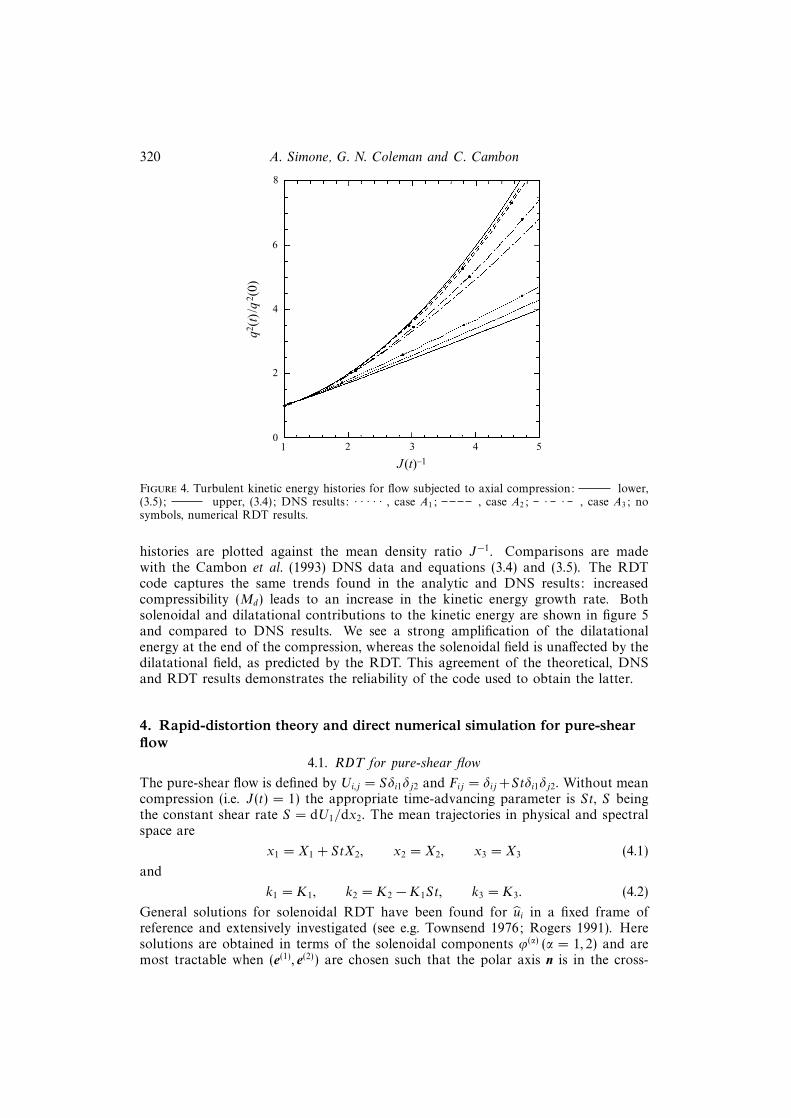
320 A. Simone, G. N. Coleman and C. Cambon
0
2
4
6
8
1 2 3 4 5
J (t)–1
q2 (t)
/q2 (
0)
Figure 4. Turbulent kinetic energy histories for flow subjected to axial compression: lower,(3.5); upper, (3.4); DNS results: · · · · · , case A1; , case A2; · · , case A3; nosymbols, numerical RDT results.
histories are plotted against the mean density ratio J−1. Comparisons are madewith the Cambon et al. (1993) DNS data and equations (3.4) and (3.5). The RDTcode captures the same trends found in the analytic and DNS results: increasedcompressibility (Md) leads to an increase in the kinetic energy growth rate. Bothsolenoidal and dilatational contributions to the kinetic energy are shown in figure 5and compared to DNS results. We see a strong amplification of the dilatationalenergy at the end of the compression, whereas the solenoidal field is unaffected by thedilatational field, as predicted by the RDT. This agreement of the theoretical, DNSand RDT results demonstrates the reliability of the code used to obtain the latter.
4. Rapid-distortion theory and direct numerical simulation for pure-shearflow
4.1. RDT for pure-shear flow
The pure-shear flow is defined by Ui,j = Sδi1δj2 and Fij = δij +Stδi1δj2. Without meancompression (i.e. J(t) = 1) the appropriate time-advancing parameter is St, S beingthe constant shear rate S = dU1/dx2. The mean trajectories in physical and spectralspace are
x1 = X1 + StX2, x2 = X2, x3 = X3 (4.1)
and
k1 = K1, k2 = K2 −K1St, k3 = K3. (4.2)
General solutions for solenoidal RDT have been found for ui in a fixed frame ofreference and extensively investigated (see e.g. Townsend 1976; Rogers 1991). Heresolutions are obtained in terms of the solenoidal components ϕ(α) (α = 1, 2) and aremost tractable when (e(1), e(2)) are chosen such that the polar axis n is in the cross-

Effect of compressibility on turbulent shear flow 321
3
2
1
1
2 3
J(t)–1
q2 s,d(t
)/q2 s(
0)
4
04 5
Figure 5. Solenoidal and dilatational turbulent kinetic energy histories for flow subjected to axialcompression: •, solenoidal; ◦, dilatational; DNS results: · · · · · , case A1; , case A2; · · ,case A3; no symbols, numerical RDT results. (Note the collapse of the solenoidal TKE histories, aspredicted by the RDT.)
gradient direction, with ni = δi2, so that e(1)2 = 0. The corresponding physical meaning
of ϕ(α) will be discussed below. Substituting the mean velocity gradient for shear flowinto (2.12), one obtains
˙ϕ(1)
+SK3
kϕ(2) =
Sk2K3
K ′y, (4.3a)
˙(k ϕ(2)) = −SK1
K ′y, (4.3b)
y + a02k2y + 2
S2K21
k4y = 2S
DDt
(K1K
′
k4
)kϕ(2), (4.3c)
z = k2y, (4.3d)
where y = ϕ(3)/k , z = ϕ(4)/a0 = ip/ρa20 (defined as in (2.17)) and K ′ = (K1
2 +K32)1/2.
Unlike for a purely irrotational mean deformation, such as the two consideredabove, the non-zero coupling between the solenoidal and dilational velocity compo-nents causes the solenoidal field to no longer be uninfluenced by the dilatational field.The dilatational–solenoidal coupling is induced whenever the mean has a rotationalcomponent, since its general form (2.13b) is mα3 = e
(α)i (Ui,j − Uj,i)e
(3)j ; for the case
of pure shear the coupling is expressed by the right-hand sides of (4.3a) and (4.3b).We shall see below that the coupling is not important at small St, and depends onlyweakly upon Md for large St, but otherwise its general behaviour is affected by Stand initial Md in a manner that is difficult to predict without obtaining full RDTsolutions.
The solenoidal limit is recovered for y = 0, and the solenoidal RDT solution

322 A. Simone, G. N. Coleman and C. Cambon
(Cambon 1982; Salhi & Cambon 1996) is relatively simple:
ϕ(1)(k, t) = ϕ1(K , 0) +KK3
K ′K1
(tan−1
(k2
K ′
)− tan−1
(K2
K ′
))ϕ(2)(K , 0), (4.4a)
ϕ(2)(k, t) =K
kϕ(2)(K , 0) . (4.4b)
Using e(1)2 = 0 and e(2)
2 = −K ′/k yields
∇2u2 = −k2u2 = −kK ′ϕ(2) − kk2ϕ(3), ω2 = −iK ′ϕ(1), (4.5a, b)
and shows that kϕ(2) and ϕ(1) are linked to the variables ∇2u2 and ω2, which aretypically the bases for studying the stability of parallel shear flow with the Orr–Sommerfeld and Squire equations. In particular, the solenoidal (y = 0, ϕ(3) = 0)solution for the ϕ(2)-equation is equivalent to conservation of ∇2u2 along meantrajectories (as shown by (4.5a) and (4.3b)).
The Md � 1 pressure-released limit is found by neglecting the second term on theleft-hand side in (4.3c), the equation governing y. This leads (for isotropic initialconditions) to quadratic amplification with respect to St of the turbulent kineticenergy,
q2(t)
q20
= 1 +(St)2
3. (4.6)
(When the initial conditions are not exactly isotropic, the pressure-released limit isgiven by q2(t)/q2
0 = 1 + (u2u2/q2)0(St)
2 − 2St(u1u2/q2)0.) A simple way to derive this
Md � 1 case is to ignore p in (2.1a) such that
u1 + Su2 = 0, u2 = u3 = 0, (4.7a, b)
and use these expressions to obtain (4.6). Note that since Du2/Dt = 0, the verticalvelocity is advected in the pressure-released limit, whereas its Laplacian is advectedin the solenoidal limit (for which D(∇2u2)/Dt = 0).
Unfortunately, the pressure-released limit yields the only easily derived analyticalsolutions for the Reynolds stress tensor. Hence numerical RDT solutions must becompared to DNS results for anything other than the Md � 1 case. The system (4.3)will be re-examined, however, in §5.
4.2. DNS for pure-shear flow
The homogeneous shear flow data used for the ensuing analysis are obtained fromDNS of the full non-isentropic compressible Navier–Stokes equations assuming spatialhomogeneity. The simulations are generated by a version of the code developed bySpyropoulos & Blaisdell (1996) (see also Blaisdell et al. 1991), which uses a pseudo-spectral spatial discretization with partial de-aliasing and a compact-storage third-order Runge–Kutta time advancement scheme. A time-dependent transformation isapplied, yielding a coordinate system that moves with the mean shearing deformation(Rogallo 1981). This allows an expansion of the solution in Fourier series, andis equivalent to the above RDT procedure of using Lagrangian coordinates andthe Fij mean-distortion tensor. Under the influence of the constant linear shearthe shape of the domain in the streamwise/cross-gradient (x, y)-plane changes froma rectangle at time zero to a parallelogram at later times (cf. figure 1d). In the
Effect of compressibility on turbulent shear flow 323
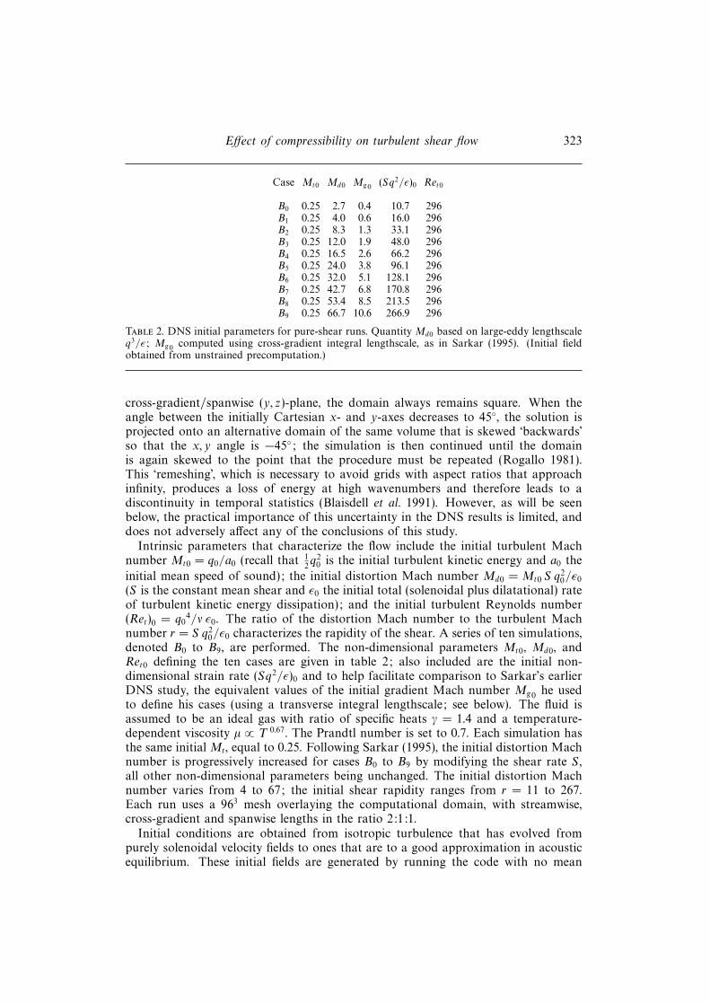
Case Mt0 Md0 Mg0 (Sq2/ε)0 Ret0
B0 0.25 2.7 0.4 10.7 296B1 0.25 4.0 0.6 16.0 296B2 0.25 8.3 1.3 33.1 296B3 0.25 12.0 1.9 48.0 296B4 0.25 16.5 2.6 66.2 296B5 0.25 24.0 3.8 96.1 296B6 0.25 32.0 5.1 128.1 296B7 0.25 42.7 6.8 170.8 296B8 0.25 53.4 8.5 213.5 296B9 0.25 66.7 10.6 266.9 296
Table 2. DNS initial parameters for pure-shear runs. Quantity Md0 based on large-eddy lengthscaleq3/ε; Mg0 computed using cross-gradient integral lengthscale, as in Sarkar (1995). (Initial fieldobtained from unstrained precomputation.)
cross-gradient/spanwise (y, z)-plane, the domain always remains square. When theangle between the initially Cartesian x- and y-axes decreases to 45◦, the solution isprojected onto an alternative domain of the same volume that is skewed ‘backwards’so that the x, y angle is −45◦; the simulation is then continued until the domainis again skewed to the point that the procedure must be repeated (Rogallo 1981).This ‘remeshing’, which is necessary to avoid grids with aspect ratios that approachinfinity, produces a loss of energy at high wavenumbers and therefore leads to adiscontinuity in temporal statistics (Blaisdell et al. 1991). However, as will be seenbelow, the practical importance of this uncertainty in the DNS results is limited, anddoes not adversely affect any of the conclusions of this study.
Intrinsic parameters that characterize the flow include the initial turbulent Machnumber Mt0 = q0/a0 (recall that 1
2q2
0 is the initial turbulent kinetic energy and a0 the
initial mean speed of sound); the initial distortion Mach number Md0 = Mt0 S q20/ε0
(S is the constant mean shear and ε0 the initial total (solenoidal plus dilatational) rateof turbulent kinetic energy dissipation); and the initial turbulent Reynolds number(Ret)0 = q0
4/ν ε0. The ratio of the distortion Mach number to the turbulent Machnumber r = S q2
0/ε0 characterizes the rapidity of the shear. A series of ten simulations,denoted B0 to B9, are performed. The non-dimensional parameters Mt0, Md0, andRet0 defining the ten cases are given in table 2; also included are the initial non-dimensional strain rate (Sq2/ε)0 and to help facilitate comparison to Sarkar’s earlierDNS study, the equivalent values of the initial gradient Mach number Mg0 he usedto define his cases (using a transverse integral lengthscale; see below). The fluid isassumed to be an ideal gas with ratio of specific heats γ = 1.4 and a temperature-dependent viscosity µ ∝ T 0.67. The Prandtl number is set to 0.7. Each simulation hasthe same initial Mt, equal to 0.25. Following Sarkar (1995), the initial distortion Machnumber is progressively increased for cases B0 to B9 by modifying the shear rate S ,all other non-dimensional parameters being unchanged. The initial distortion Machnumber varies from 4 to 67; the initial shear rapidity ranges from r = 11 to 267.Each run uses a 963 mesh overlaying the computational domain, with streamwise,cross-gradient and spanwise lengths in the ratio 2:1:1.
Initial conditions are obtained from isotropic turbulence that has evolved frompurely solenoidal velocity fields to ones that are to a good approximation in acousticequilibrium. These initial fields are generated by running the code with no mean

324 A. Simone, G. N. Coleman and C. Cambon
straining for about 2 units of ‘eddy turn-over time’ q2/ε (measured in terms ofquantities at the time the shear is applied), until they develop realistic triple-velocitycorrelations and dilatational energy for the given turbulent Mach number. Thiswould be unnecessary if we were only interested in asymptotic behaviour (such asthe Md dependence at large St examined by Sarkar 1995), since the later stages ofsheared homogeneous compressible turbulence evolve to become independent of theinitial data, allowing one to apply the shear directly to ‘unphysical’ initial conditions(Blaisdell et al. 1991; Sarkar 1995). But since here our interest is in both early andlate times, the unstrained ‘precomputations’ are required. They begin from uniformdensity and pressure fields, and a random solenoidal velocity field, all of whose spectraare proportional to E(k) = k4 exp (−2 k2/k2
p); the peak wavenumber, kp, locates themaximum initial value of the spectra, and is chosen such that kpLy/2π = 8, whereLy is the size of the domain in the cross-gradient (and spanwise) direction. Choosingthis relatively small value of kp allows us to obtain Reynolds numbers larger thanif kp had been larger (cf. Blaisdell et al. 1993; Sarkar 1995); however, because thestreamwise lengthscales of the turbulence grow under the influence of the shear, thismeans that the periodic boundary conditions affect the solution sooner than theywould for a larger-kp computation. Consequently, we have taken care to ensure thatthe DNS results presented below are independent of the domain size.
In order to explore the relevance of the RDT to Sarkar’s (1995) DNS results,two of the simulations, cases B1 and B2, are respectively similar to his runs A3
and A4. The initial Md is thus chosen to be 4 for case B1 and 8.3 for case B2.Because our measure of the shear rapidity is based on the large-eddy lengthscale` = q3/ε, instead of the integral lengthscale of the velocity in the transverse shearing(cross-gradient) direction used by Sarkar to compute his gradient Mach numberMg , these values of Md closely correspond to the Mg of 0.66 and 1.32 of his runsA3 and A4, respectively. (As we shall see, these two simulations by Sarkar can beconsidered as falling within the rapid-distortion regime, in the sense that they giveresults that are closely approximated by RDT solutions that use his case A3 and A4
parameters.) Although for the parallel B1/A3 and B2/A4 cases the effective initialdistortion Mach numbers are approximately the same, the turbulent Mach numbersMt for Sarkar’s and the present results are not. This is mainly a consequence ofchoosing to employ fully developed initial conditions; since a finite time is requiredfor the unstrained precomputation to develop realistic turbulence, and during thistime the turbulent Mach number rapidly decays, the initial turbulent Mach numberused here, Mt0 = 0.25, is smaller than the constant Mt0 = 0.4 employed by Sarkar.However, when the distortion Mach numbers match, because the initial Mt for theprevious and present DNS are of the same order, so are the initial Mg/Mt ratios.Because the peak in the initial spectra was chosen to be at a fairly low wavenumber,kp = 16π/Ly , the turbulent Reynolds number Ret ≈ 300 of the initial field generatedby the precomputation is significantly larger than the initial Ret ≈ 200 used bySarkar. Spectra were examined to verify that at this Reynolds number the 963-gridis sufficient to accurately resolve both the initial and sheared turbulent fields. It wasmentioned earlier that during the computations the integral lengthscales grow so thateventually the large eddies fill the computational domain and the simulations becomeinvalid. The density integral-lengthscale is a good measure of whether or not this hashappened (Blaisdell et al. 1991). Accordingly, the two-point correlation of the densityfield was monitored to verify that the solutions are not adversely influenced by theperiodic boundary conditions before the time at which each simulation was stopped,which varied between St = 10 and 15.

Effect of compressibility on turbulent shear flow 325
10
8
6
4
2
0 5 10 15
St
q2 (t)
/q2 (
0)
Figure 6. Turbulent kinetic energy histories for pure-shear flow: , (4.6); · · · · · , DNS withinitial Md ranging from 4 (lower) to 67 (upper). Arrow shows trend with increasing Md.
4.3. Numerical RDT and DNS results
Histories of the total turbulent kinetic energy from the DNS are presented in figure 6,plotted against the non-dimensional shear rate St. (The discontinuity at odd valuesof St is caused by the remeshing procedure, explained above.) As predicted by theRDT analysis in §4.1, we find that all the curves are bounded by the pressure-released(Md � 1) limit represented by the solid curve. The rate of energy amplificationmonotonically increases with initial Md, at low St, and becomes linear at large St.The linear growth rate is much smaller, however (by about a factor of three forthe lowest-Md DNS run at St ≈ 12, for example) than the large-St RDT predictionfor the incompressible case, ∂
(q2/q2(0)
)/∂(St) ∼ 2 ln 2 (Rogers 1991). In fact,
both the asymptotic incompressible RDT solution and that at general St consistentlyoverpredict the magnitude of q2(t)/q2(0) observed in the compressible DNS. However,we shall subsequently see that the history of the TKE production rate given by thesolenoidal RDT analysis is relevant to the fully compressible flow.
The development of the temporal growth rate of the turbulent kinetic energy isshown in figures 7(a) and 7(b) (only DNS results not directly affected by the remeshingdiscontinuity are included), and will be discussed further below. (The oscillations inthe DNS results are due to the statistical uncertainty associated with the limitedsample provided by a domain of finite size, while the slight ‘waviness’ at large timesin the RDT histories is the result of the wavenumber discretization (equidistant inlog k, see Cambon 1982; Benoit 1992) needed to solve (2.12), and also the difficulty inresolving at large wavenumber the high frequencies ak introduced at large St.) The

326 A. Simone, G. N. Coleman and C. Cambon
0.6
(a)
0.4
0.2
0 5 10 15St
K
0.6
(b)
0.4
0.2
0 5 10 15St
K
Figure 7. Histories of the temporal energy growth rate for pure-shear flow: , (4.9); (a) · · · · · ,DNS; (b) · · · · · , RDT. Initial Md ranges from 4 to 67 for both DNS and RDT; arrows show trendwith increasing Md.
growth rate is defined by the non-dimensional parameter (as in Sarkar’s paper)
Λ =1
SKdKdt
, (4.8)
where K = 12q2. Figure 7 indicates that for St < 4 the growth rate increases with
initial distortion Mach number Md0 and tends toward the pressure-released limit

Effect of compressibility on turbulent shear flow 327
0.6
0.4
0.2
K
0.8
1 2 3 4 5
J(t )–1
Figure 8. RDT histories of the temporal energy growth rate for one-dimensional axially compressedflow: , analytic RDT limits: lower, pure-solenoidal regime; upper, pressure-released regime;· · · · · , case A1,; , case A2; · · , case A3.
(solid curve) given by
Λpr =2St
3 + (St)2, (4.9)
which represents the maximum growth rate, found for initial Md0 � 1. However, thetrend is reversed at larger St: Λ decreases with increasing Md0. It is noteworthy thatall the curves exhibit this transition from increasing to decreasing growth rate withMd near St ≈ 4 or 5. This ‘crossover’ feature can only exist when the mean velocityfield is rotational; to illustrate, RDT histories of the temporal energy growth rate forthe one-dimensional axisymmetric compression discussed above (cases A1 to A3) arepresented in figure 8. Here Λ is observed to scale monotonically with Md0, whichvaries from 0 for the lower solid curve, to 5 for the dotted, 29 for the chain-dotted,87 for the dashed, and infinity for the upper solid curve (the two theoretical curves– the Md = 0 solenoidal and Md → ∞ pressure-released limits – being obtained bytaking the time derivative of (3.5) and (3.4), respectively). The implication is thatthe crossover is due to the coupling of the solenoidal and dilatational velocity fieldsmediated by mα3, which is equal to zero if the mean flow is irrotational.
What is thought to be one of the most noteworthy results of this study is found infigure 7, which shows that the general Md dependence observed in the homogeneous-shear DNS is also present in the RDT. Although there are some quantitative dif-ferences between the RDT and DNS data (the DNS growth rates are consistentlysmaller than those predicted by the RDT, and consequently the asymptotic values ofΛ at large St are not the same), in general the agreement is quite striking, even in theapproximate location of the St ≈ 4 crossover transition.
Continuing our examination of the DNS and RDT results and their implications,we next use (1.4) to derive the exact equation for the evolution of Λ in homogeneous

328 A. Simone, G. N. Coleman and C. Cambon
0.6
0.4
0.2
0 5 10 15St
(a)
–2 b12
0.6
0.4
0.2
0 5 10 15St
(b)
–2 b12
Figure 9. Histories of the non-dimensional production term −2b12 for pure-shear flow: (a) · · · · · ,DNS; (b) · · · · · , RDT; lower, incompressible run performed using the incompressible-flowversion of MITHRA; upper, pressure-released limit. Initial Md ranges from 4 to 67 for bothDNS and RDT; arrows show trend with increasing Md.
shear flow:
Λ = −2b12 −εs + εd −Πd
SK
= −2b12
(1− εs + εd −Πd
P
)= −2b12(1− χε), (4.10)
where b12 = u1u2/2K = −P/2SK is the relevant component of the Reynolds
Effect of compressibility on turbulent shear flow 329
0
1
2
3
5 10 15St
(ε–πd)/0
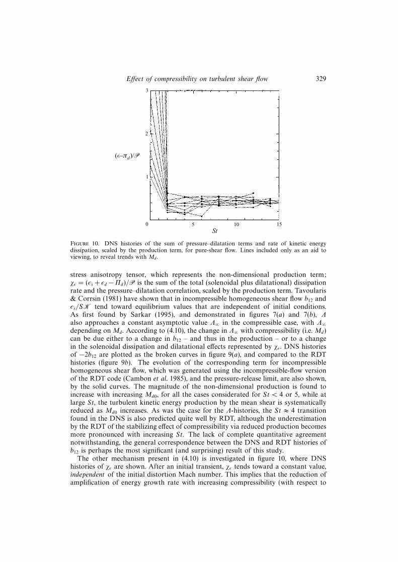
Figure 10. DNS histories of the sum of pressure–dilatation terms and rate of kinetic energydissipation, scaled by the production term, for pure-shear flow. Lines included only as an aid toviewing, to reveal trends with Md.
stress anisotropy tensor, which represents the non-dimensional production term;χε = (εs + εd−Πd)/P is the sum of the total (solenoidal plus dilatational) dissipationrate and the pressure–dilatation correlation, scaled by the production term. Tavoularis& Corrsin (1981) have shown that in incompressible homogeneous shear flow b12 andεs/SK tend toward equilibrium values that are independent of initial conditions.As first found by Sarkar (1995), and demonstrated in figures 7(a) and 7(b), Λalso approaches a constant asymptotic value Λ∞ in the compressible case, with Λ∞depending on Md. According to (4.10), the change in Λ∞ with compressibility (i.e. Md)can be due either to a change in b12 – and thus in the production – or to a changein the solenoidal dissipation and dilatational effects represented by χε. DNS historiesof −2b12 are plotted as the broken curves in figure 9(a), and compared to the RDThistories (figure 9b). The evolution of the corresponding term for incompressiblehomogeneous shear flow, which was generated using the incompressible-flow versionof the RDT code (Cambon et al. 1985), and the pressure-release limit, are also shown,by the solid curves. The magnitude of the non-dimensional production is found toincrease with increasing Md0, for all the cases considerated for St < 4 or 5, while atlarge St, the turbulent kinetic energy production by the mean shear is systematicallyreduced as Md0 increases. As was the case for the Λ-histories, the St ≈ 4 transitionfound in the DNS is also predicted quite well by RDT, although the underestimationby the RDT of the stabilizing effect of compressibility via reduced production becomesmore pronounced with increasing St. The lack of complete quantitative agreementnotwithstanding, the general correspondence between the DNS and RDT histories ofb12 is perhaps the most significant (and surprising) result of this study.
The other mechanism present in (4.10) is investigated in figure 10, where DNShistories of χε are shown. After an initial transient, χε tends toward a constant value,independent of the initial distortion Mach number. This implies that the reduction ofamplification of energy growth rate with increasing compressibility (with respect to
330 A. Simone, G. N. Coleman and C. Cambon
–0.2
0.4
0.2
0
5 10 15St
–2 bs12
0.6
0.4
–0.2
0
5 10 15St
(b)
(a)
0
–2 bs12
0
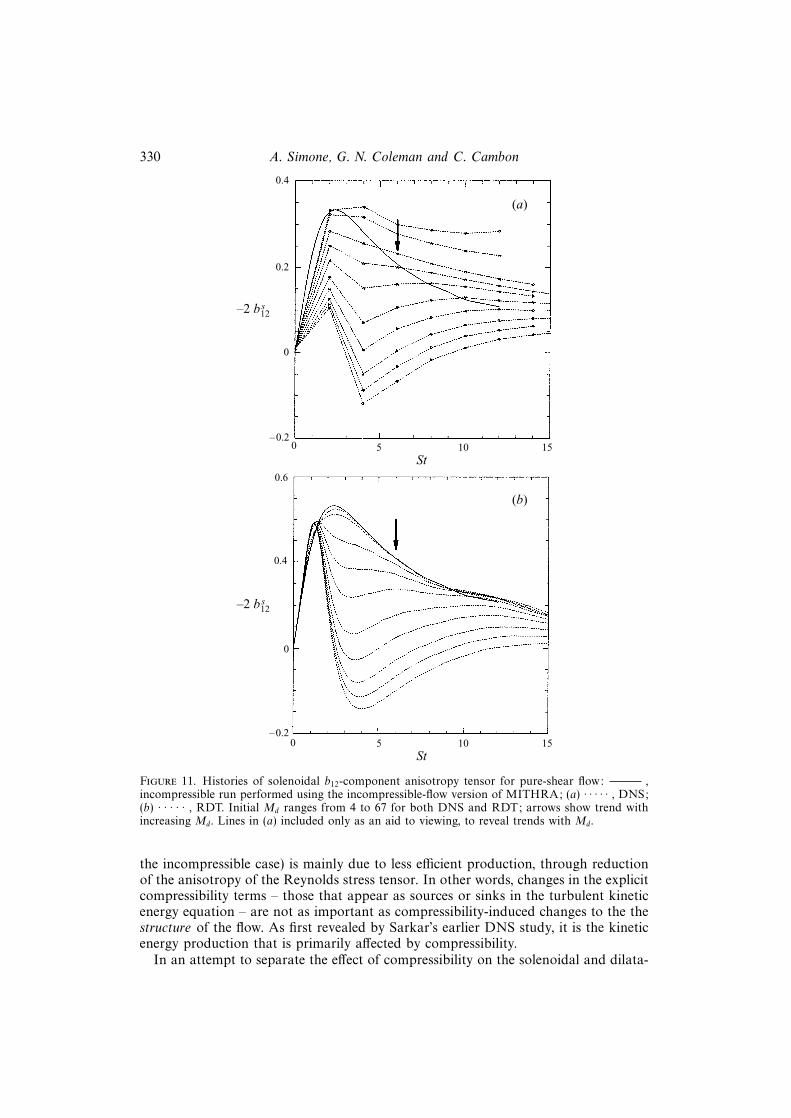
Figure 11. Histories of solenoidal b12-component anisotropy tensor for pure-shear flow: ,incompressible run performed using the incompressible-flow version of MITHRA; (a) · · · · · , DNS;(b) · · · · · , RDT. Initial Md ranges from 4 to 67 for both DNS and RDT; arrows show trend withincreasing Md. Lines in (a) included only as an aid to viewing, to reveal trends with Md.
the incompressible case) is mainly due to less efficient production, through reductionof the anisotropy of the Reynolds stress tensor. In other words, changes in the explicitcompressibility terms – those that appear as sources or sinks in the turbulent kineticenergy equation – are not as important as compressibility-induced changes to the thestructure of the flow. As first revealed by Sarkar’s earlier DNS study, it is the kineticenergy production that is primarily affected by compressibility.
In an attempt to separate the effect of compressibility on the solenoidal and dilata-

Effect of compressibility on turbulent shear flow 331
tional contributions to the turbulent kinetic energy, the Helmholtz decomposition ofthe fluctuating velocity field was used for the pure shear as well as the one-dimensionalcompression flow; no evidence of scaling with Md0 was found. However, decompo-sition of the b12 component of the anisotropy tensor into solenoidal and dilatationalcomponents defined by
bij(s)(t) =
Rij(s)(t)
q2s (t)
− δij
3, bij
(d)(t) =Rij
(d)(t)
q2d(t)
− δij
3(4.11a, b)
(where R(s)ij = usi u
sj and R
(d)ij = udi u
dj ) is more fruitful. Histories of these terms are
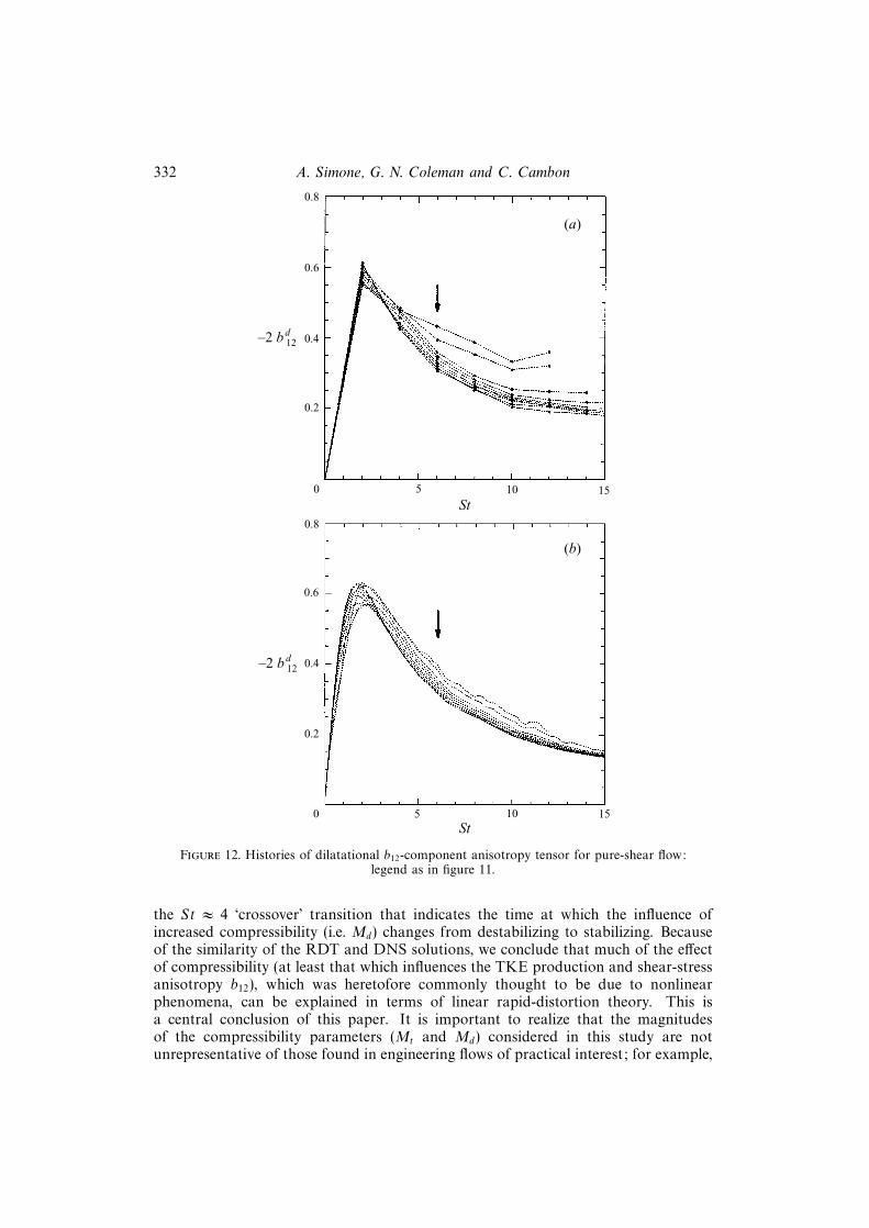
shown in figures 11 and 12, respectively. We see that the solenoidal contribution isdramatically decreased over the entire range of St whereas the dilatational one isessentially unaffected by compressibility. The structure alteration mentioned aboveis therefore due almost entirely to changes in the solenoidal field. For all the casesconsidered both contributions approach constant equilibrium values at large St. TheRDT predicts that the dilatational component is essentially independent of Md for allvalues of St, while the solenoidal component exhibits a pronounced Md dependenceover the entire range of times shown, with the strong suggestion of collapse to aunique value (independent of Md), as St → ∞. The DNS results, on the other hand,while showing the same general trends as the RDT histories do, tend to be moresensitive to Md, with the large-St limits of both b
(s)12 and b
(d)12 depending upon the
initial distortion Mach number. This difference between the RDT and DNS results isprobably due to the nonlinear and dissipative terms that are present in the DNS; theimportance of these terms will be discussed in the next section.
5. Discussion and conclusions5.1. General comments
The objective of this work has been to develop a general RDT code capable ofsolving linearized equations valid for compressible homogeneous turbulence for alarge range of the two compressibility parameters important for turbulence subjectedto mean shear, Mt and Md. Two types of mean uniform velocity gradients (sphericalcompression and one-dimensional axisymmetric compression) have been examined inorder to validate the numerical code; results of the RDT code have been comparedwith analytical solutions and DNS data at high compression speed, and have demon-strated good agreement. The pure plane-shear flow was then investigated and RDTand DNS results have been presented and discussed in the light of recent simulationsperformed by Sarkar (1995). As in his earlier study, we find that changes in the‘structure’ of the turbulence (i.e. altered production of turbulent kinetic energy) aremuch more significant than changes associated with the new (compressibility-induced)source terms in the turbulent kinetic energy equation.
When viewed separately, the primary value of the RDT and DNS results presentedhere is solely to reconfirm (and extend the range of validity for) many of Sarkar’searlier findings regarding the structure-altering role of compressibility in homogeneoussheared turbulence. However, when they are viewed together, their broad generalagreement reveals the extent to which the structural alterations are governed bylinear processes. Although the agreement is not exact (for example, in the St → ∞asymptotic limits predicted for Λ and b12), many of the RDT and DNS results aresurprisingly close to each other. In particular, we note that at early times the RDTand DNS histories are very similar, and especially that the RDT correctly locates
332 A. Simone, G. N. Coleman and C. Cambon
0.4
0.2
5 10 15St
–2 bd12
0.8
0.4
0.2
0 5 10 15St
(b)
(a)
0
–2 bd12
0.6
0.6
0.8
Figure 12. Histories of dilatational b12-component anisotropy tensor for pure-shear flow:legend as in figure 11.
the St ≈ 4 ‘crossover’ transition that indicates the time at which the influence ofincreased compressibility (i.e. Md) changes from destabilizing to stabilizing. Becauseof the similarity of the RDT and DNS solutions, we conclude that much of the effectof compressibility (at least that which influences the TKE production and shear-stressanisotropy b12), which was heretofore commonly thought to be due to nonlinearphenomena, can be explained in terms of linear rapid-distortion theory. This isa central conclusion of this paper. It is important to realize that the magnitudesof the compressibility parameters (Mt and Md) considered in this study are notunrepresentative of those found in engineering flows of practical interest; for example,

Effect of compressibility on turbulent shear flow 333
based on the analysis of Sarkar (1995), we estimate that the distortion Mach numbersemployed for cases B1 and B2 (cf. table 2) correspond to convective Mach numbersfound in a compressible mixing layer of less than one (see his figure 14). The presentstudy therefore appears to be much more relevant than one might expect of ananalysis based on rapid-distortion assumptions. Given this relevance, we now turnour attention to its broader implications.
5.2. The ‘stabilizing’ effect of compressibility revisited
A comparison of the development of the growth-rate parameter Λ between RDTresults for axisymmetric compression (figure 8) and pure shear (figure 7a, b) illustratesthat increases in the distortion Mach number can cause the turbulence to becomeeither more or less energetic, depending upon both the type of mean deformation andthe time at which the flow is examined. In this section, we attempt to clarify the reasonsfor, and the conditions that produce, both the stabilizing and destabilizing influenceof compressibility. We begin by considering deformations for which increasing Md
always causes the flow to become more energetic.
5.2.1. Irrotational distortions
Intrinsic compressibility is destabilizing – in the sense that it leads to generationof greater turbulent kinetic energy than when the velocity fluctuations are purelysolenoidal – for all rapid irrotational mean distortions, throughout the history ofthe flow; because the solenoidal field is unaffected by an irrotational deformation,the sum of the solenoidal and dilatational kinetic energy will always be greater thanthat found for the purely solenoidal case. This can be understood, without having toutilize a Fourier representation, from the general solution of the linearized equations,
ui(x, t) = F−1ji (X , t, 0) uj(X , 0)︸ ︷︷ ︸
Vi=V(s)i
+V(d)i
+∂ φ
∂xi, (5.1a)
φ = p/ρ, (5.1b)
which is valid even for inhomogeneous flows. Equation (5.1) was extensively used byGoldstein (1978) and Durbin & Zeman (1992), among others (the present notationfollows that of Cambon 1982 and Cambon et al. 1985, 1993). The first term on theright-hand side of (5.1a) can be split into a solenoidal and a dilatational part (via theHelmholtz decomposition), such that F−1
ji (uj)0 = Vi = V(s)i +V (d)
i ; the dilatational partis present for any anisotropic mean strain even if the initial velocity field is solenoidal.Accordingly, the other term in (5.1a), which involves the pressure fluctuation, exactlybalances the dilatational part V (d)
i in the solenoidal limit Md → 0, and is zero in thepressure-released regime (Md → ∞). In other words, Vi is the pressure-released RDTsolution, and V (s)
i denotes the solenoidal RDT solution:
usi = V(s)i , udi = V
(d)i + φ,i. (5.2a, b)
The transition with increasing Md from the solenoidal to the pressure-released solutionaccompanies the progressive emergence of udi , as V (d) is less and less balanced byφ,i, at fixed (since it is unaffected by compressibility) usi . This suggests the simpleparameterization:
ui = Vi + f(Md) (V (s)i − Vi), (5.3)
where f(Md) is a monotonic function that varies from 1 to 0 as Md varies from0 (representing the solenoidal solution) to infinity (yielding the pressure-released

334 A. Simone, G. N. Coleman and C. Cambon
solution), with Vi = F−1ji (uj)0 and its solenoidal projection V
(s)i being determined by
the Lagrangian distortion tensor and the initial conditions only. (Such a weighting-function parameterization was suggested in a modified model for pressure–straincorrelations by Cambon et al. 1993.) This simple analysis is sufficient to explain themain compressibility effects in RDT for irrotational mean flows. Further analysis,however, requires the use of Fourier space in order to decompose Vi into V (s)
i +V(d)i in
a tractable form, and especially to study the coupled system of equations governingudi and p, (2.18) and (2.19).
5.2.2. Vortical distortions: the pure shear
The above simple analysis is no longer possible if the mean distortion has a vorticalpart. The Weber–Goldstein equation (5.1) is no longer valid, and the complete system(2.12) must be considered. However, the pure-shear RDT and DNS results shownabove nevertheless exhibit the destabilizing trend predicted by (5.3), but only at smallSt. At later times, for St greater than about 4, behaviour opposite to that implied bythe analysis in the previous section is found (figure 7). The reason for this transitionof the influence of compressibility from being destabilizing to being stabilizing willnow be sought.
The essential difficulty in trying to analytically solve the linear system of RDTequations (4.3) for pure shear comes from the time-dependent character of thecoefficients that contain k(t) (see (4.2)). Only when k1 = 0 does this time-dependencedisappear, so that (4.3) is drastically simplified, yielding an oscillatory solution fory (as in the acoustic unsheared case), and the pure-solenoidal solution for ϕ(2). Fork1 6= 0 we focus on the restricted system of equations for ϕ(i), with i = (2, 3, 4) only:
ξ = SK1k2y, y = −2S
K1
k4ξ − a2
0z, z = k2y, (5.4a–c)
where y = ϕ(3)/k and z = ϕ(4)/a0 are defined as in (4.3), and ξ = −kK ′ϕ(2) is theFourier transform of the solenoidal part of ∇2u2, as shown in (4.5a). Only the vertical(i.e. cross-gradient) velocity component (through ξ and y) and the pressure (throughz) are present in the above, and the time-dependence of the coefficient is solelythrough k2(t). Because the time-dependent parts of the right-hand side of both (5.4a)and (5.4c) are in k2y, the new variable
Z = z − ξ
SK1
(5.5)
is time-invariant (Z = 0), and can replace z in the set of variables. Thus, in terms ofZ, ξ and y, the previous system can be written
Z = 0, ξ = SK1k2y, y = −
(2SK1
k4+
a20
SK1
)ξ − a2
0Z. (5.6a–c)
The latter equation is the key to understanding the time-dependence of (linear) com-pressibility effects in turbulent shear flow; this is done by comparing the magnitude ofthe two terms in the ξ-coefficient in (5.6c): the first one, 2SK1/k
4, rapidly approacheszero as St increases (provided K1 6= 0; if K1 = 0, it vanishes), whereas the secondone, a2
0/(SK1), remains constant. Hence, if St is sufficiently large, the inequality2SK1/k
4 � a20/(SK1) holds, such that
2S2`2
a20
�[1 +
K23
K21
+K2
2
K21
− 2K2
K1
St+ (St)2
]2
(K1`)2, (5.7)
Effect of compressibility on turbulent shear flow 335
where (4.2) has been used to express the magnitude of the time-dependent wavenumberin terms of its initial components, K1, K2 and K3, and here ` is the lengthscalepreviously defined. Equation (5.7) is roughly equivalent to Md � (St)2 for large St,
which defines the ‘large-St’ criterion as being St�M1/2d (assuming that the ‘average’
magnitude of the components of K that significantly contribute to the energy are ofthe order 1/`).
The ‘crossover’ behaviour cited above can be related to the change of regimecaused by passing from small St – where 2SK1/k
4 is relevant and can be dominantwith respect to a2
0/(SK1) at sufficiently large Md – to large St, where 2SK1/k4 is
never significant, even at large Md. In the latter, even if the initial conditions arecharacterized by large Md, the asymptotic state will be essentially independent of Md,since the 2SK1/k
4 term can be neglected in (5.6c), which can then be differentiatedwith respect to time to yield the simplified equation y+a2
0k2y = 0. Although k2 varies
strongly with time in this equation, an oscillating (and thus bounded) solution for ycan be inferred using a WKB-type argument (ω = a0k; ω/ω
2 becomes small at largeSt). Hence the behaviour at large St and that previously referred to as quasi-acousticor quasi-solenoidal are similar. Considering the dynamic behaviour at sufficientlylarge St, with solenoidal RDT one can compare the fixed points (ξ = y = 0) of thesimplified system (5.6a–c) obtained by dropping the 2SK1/k
4 term. We find
ξ = ξ0 − SK1z0, y = 0, z = 0. (5.8)
The corresponding RDT solution in the pure-solenoidal case is
ξ = ξ0, y = 0, a20z = a2
0zs = 2S
K1
k4ξ0. (5.9)
Note that z = zs is equivalent to the classic Poisson equation, as in (2.19)–(2.20),and zs is precisely the term that is neglected in (5.6c) at large St. It is importantto point out that ξ0 = ξ(X , 0) is an ‘initial’ condition chosen at any time for thepure-solenoidal case, whereas ξ0, z0 for the fixed-point solution (5.8) can be viewed as‘initial’ data chosen at a time (after the crossover) for which the inequality (5.7) holds.The post-crossover state at intermediate St depends on the entire history, which isinfluenced by Md during the early history of the flow.
This semi-analytical analysis can explain the change of regime passing from smallto large St. It cannot, however, explain why the crossover occurs near St ≈ 4, for allMd, and why, after the crossover, increasing Md causes the stabilization of the flowrevealed by the RDT and DNS results. Two characteristics of the RDT equationscan perhaps shed light on the matter:
(i) The first is the time-dependency of the wave vector, which physically reflects thekinematic distortion of a material bipoint (linear fluid element) li(t) advected by theshear flow, in accordance with a wave-conservation law kili = constant (see (2.14)).Consequently, the wavevector is primarily stretched (such that |k| increases) and itsorientation becomes more and more vertical, due to the increase of k2. This pure-advection effect tends to transfer energy toward smaller and smaller scales, which areless and less affected by compressibility (see e.g. figure 1 in Cambon et al. 1993 andthe related discussion).
(ii) The second characteristic is the coupling term induced by the vortical part ofthe mean deformation (see (2.12) and (4.3a, b)). Even though the distortion of thewavevector also exists in an irrotational mean flow, this coupling term does not; thisimplies that it plays an essential role in the pure-shear crossover behaviour, althoughthe coupling is less important at very small St (where the influence of the pure-

336 A. Simone, G. N. Coleman and C. Cambon
straining irrotational part of the shear comes into play) and at very large St, for thereasons given earlier in this section. Although for pure-shear flow the most importanteffect of compressibility (in the rapid-distortion regime) is to alter the structure ofthe solenoidal fluctuations, as reflected in the Md-dependence of b(s)
12 (figure 11b), theultimate source of this alteration is the feedback of the dilatational disturbances uponthe solenoidal field – since in a non-vortical mean flow the solenoidal fluctuations arecompletely independent of Md, and are equivalent to those found in the ui,i = 0 case.
5.2.3. Nonlinear and dissipative effects
By comparing the RDT and DNS results presented above (see e.g. the b12-historiesin figure 9), one finds that much of the structural effect of compressibility is fairly wellreproduced by the linear rapid-distortion analysis. This is especially true during theinitial development of the flow, for a range of time that extends past that (St ≈ 4) atwhich the destabilization-to-stabilization change in the role of compressibility occurs.At later times, however, as St → ∞, the DNS histories exhibit a dependence upondistortion Mach number that is not captured by the RDT. Although the asymptoticnon-dimensional production b12 predicted by the RDT appear to be converging toa unique value, independently of initial Md (figure 9b) (which is consistent withthe simplified fixed-point analysis in §5.2.2), the same cannot be said for the fullnonlinear solutions (figure 9a). Evidently, nonlinear and dissipative effects (thedissipative scales receiving energy through the nonlinear cascade) are not essential forpredicting the general trends, although they are important in breaking the reversibilityof linear solutions, causing a dependence on the compressibility parameter Md of theasymptotic results.
Some authors (e.g. Friedrich 1996) have recently pointed out that the dilatationaldissipation tensor εdij is strongly anisotropic in shear flows, with the vertical compo-
nent εd22 being dominant. While a major theme of this paper has been the irrelevance(compared to alteration of the turbulent kinetic energy production) of the rate ofdilatational dissipation of turbulent kinetic energy εd = 1
2εdii, one of the compo-
nents (i.e. εd22) becoming dominant with respect to the others could lead to furthermodification of the Reynolds stress tensor, and thereby cause a further ‘stabilizing’influence associated with compressibility. Although the RDT-based explanation ofcompressibility effects offered here and that attributed to anisotropy of the dilata-tional dissipation do not correspond, it is perhaps significant that both focus on thebehaviour of the vertical (cross-gradient) components of the quantities of interest– be they velocity fluctuations, Reynolds stress tensors, or dissipation tensors. Therecent DNS results analysed by Speziale et al. (1995) also suggest that a detailedcomparison of the components of various anisotropy measures predicted by RDTand DNS might be a fruitful endeavour.
We are grateful to Professor G. A. Blaisdell and E. T. Spyropoulos for helpful sug-gestions and for allowing us to use their DNS code. Financial support for the firstauthor was supplied by DRET (Direction des Recherches, Etudes et Techniques,DGA, French Defense), under contract 95/2585 A (Recherche fondamentale). Com-putational resources were made available on the Cray 98 by IDRIS (Institut deDeveloppement et des Ressources en Informatique Scientifique), which receives majorfunding from the CNRS.

Effect of compressibility on turbulent shear flow 337
REFERENCES
Batchelor, G.K. & Proudman, I. 1954 The effect of rapid distortion of a fluid in turbulent motion.Q. J. Mech. Appl. Math. 7, 121–152.
Benoit, J. P. 1992 Etude experimentale et theorique d’une turbulence homogene soumise a des effetscouples de rotation et de deformation. These de Doctorat, Universite Claude Bernard Lyon I,France.
Blaisdell, G.A., Coleman, G.N. & Mansour, N.N. 1996 Rapid distortion theory for compressiblehomogeneous turbulence under isotropic mean strain. Phys. Fluids 8, 2622–2705
Blaisdell, G.A., Mansour, N.N. & Reynolds, W.C. 1991 Numerical simulation of compressiblehomogeneous turbulence. Dept of Mech. Engng, Stanford University, Thermosciences Div. Rep.TF-50.
Blaisdell, G.A., Mansour, N.N. & Reynolds, W.C. 1993 Compressibility effects on the growthand structure of homogeneous turbulent shear flow. J. Fluid Mech. 256, 443–485.
Bradshaw, P. 1977 Compressible turbulent shear layers. Ann. Rev. Fluid Mech. 9, 33–54.
Cambon, C. 1982 Etude spectrale d’un champ turbulent incompressible soumis a des effets couples
de deformation et de rotation imposes exterieurement. These d’Etat, Universite Claude BernardLyon I, France.
Cambon, C., Benoit, J. P., Shao, L. & Jacquin, L. 1994 Stability analysis and large eddy simulationof rotating turbulence with organized eddies. J. Fluid Mech. 278, 175–200.
Cambon, C., Coleman, G.N. & Mansour, N.N. 1993 Rapid distortion analysis and direct sim-ulation of compressible homogeneous turbulence at finite Mach number. J. Fluid Mech. 257,641–665.
Cambon, C., Teissedre, C. & Jeandel, D. 1985 Etude d’effets couples de deformation et de rotationsur une turbulence homogene. J. Mec. Theor. Appl. 4, 629–657
Clemens, N. T. & Mungal, M.G. 1995 Large-scale structure and entrainment in the supersonicmixing layer. J. Fluid Mech. 284, 171–216.
Durbin, P. A. & Zeman, O. 1992 Rapid distortion theory for homogeneous compressed turbulencewith application to modelling. J. Fluid Mech. 242, 349–370.
Eringen, A. C. 1980 Mechanics of Continua. Wiley.
Fernholz, H.H. & Finley, P. J. 1977 A critical compilation of compressible turbulent boundarylayer data. AGARDograph 223.
Fernholz, H.H. & Finley, P. J. 1980 A critical commentary on mean flow data for two-dimensionalcompressible turbulent boundary layers. AGARDograph 253.
Fernholz, H.H., Smits, A. J., Dussauge, J.-P. & Finley, P. J. 1989 A survey of measurements andmeasuring techniques in rapidly distorted compressible turbulent boundary layers. AGARDo-graph 315.
Friedrich, R. 1993 Compressible turbulence. Lehrstuhl fur Fluidmechanik, Technische UniversitatMunchen, Space Course 1993 class notes.
Friedrich, R. 1996 Compressibility effects due to turbulent fluctuations. Eur. Turb. Conf. 6, Lau-sanne, 2-5 July 1996, Invited lecture.
Goldstein, M. E. 1978 Unsteady vortical and entropic distortions of potential flows round arbitraryobstacles. J. Fluid Mech. 89, 433–468.
Huang, P.G., Coleman, G.N. & Bradshaw, P. 1995 Compressible turbulent channel flows: DNSresults and modelling. J. Fluid Mech. 305, 185–218.
Jacquin, L., Cambon, C. & Blin, E. 1993 Turbulence amplification by a shock wave and rapiddistortion theory. Phys. Fluids A 10, 2539–2550.
Kevlahan, N.K.R. & Hunt, C. J. R. 1996 Nonlinear interactions in turbulence with strong irrota-tional straining. Submitted to J. Fluid Mech.
Kovasznay, L. S.G. 1953 Turbulence in supersonic flow. J. Aeronaut. Sci. 20, 657–682.
Lee, S., Lele, S.K. & Moin, P. 1993 Direct numerical simulation of isotropic turbulence interactingwith a weak shock wave. J. Fluid Mech. 251, 533–562.
Lele, S.K. 1994 Compressibility effects on turbulence. Ann. Rev. Fluid Mech. 26, 211–254.
Marion, J. D. 1988 Etude spectrale d’une turbulence isotrope compressible. These de Doctorat,Ecole Centrale de Lyon, France.
Monin, A. S. & Yaglom, A.M. 1971 Statistical Fluid Mechanics: Mechanics of Turbulence. The MITPress.
338 A. Simone, G. N. Coleman and C. Cambon
Papamoschou, D. & Roshko, A. 1988 The compressible turbulent mixing layer: an experimentalstudy. J. Fluid Mech. 197, 453–477.
Rogallo, R. S. 1981 Numerical experiments in homogeneous turbulence. NASA TM–81315.
Rogers, M.M. 1991 The structure of a passive scalar field with a uniform mean gradient in rapidlysheared homogeneous turbulent flow. Phys. Fluids A 3, 144–154.
Salhi, A. & Cambon, C. 1996 A new analysis of rotating shear flows using linear approach andDNS-LES results. Submitted to J. Fluid Mech.
Sandham, N.D. & Reynolds, W.C. 1991 Three-dimensional simulations of large eddies in thecompressible mixing layer. J. Fluid Mech. 224, 133–158.
Sarkar, S. 1995 The stabilizing effect of compressibility in turbulent shear flow. J. Fluid Mech. 282,163–186.
Sarkar, S., Erlebacher, G. & Hussaini, M.Y. 1991a Direct simulation of compressible turbulencein a shear flow. Theoret. Comput. Fluid Dyn. 2, 291–305.
Sarkar, S., Erlebacher, G., Hussaini, M.Y. & Kreiss, O. 1991b The analysis and modelling ofdilatational terms in compressible turbulence. J. Fluid Mech. 227, 473–493.
Settles, G. S. & Dodson, L. J. 1991 Hypersonic shock/boundary layer interaction database. NASAContractor Rep. 177577.
Simone, A. 1995 Etude theorique et simulation numerique de la turbulence compressible en presencede cisaillement ou de variation de volume a grande echelle. These de Doctorat, Ecole Centralede Lyon, France.
Simone, A. & Cambon, C. 1995a Revisiting compressible homogeneous shear flow at finite Machnumber by means of rapid distortion theory. Proc. Fifth European Turbulence Conf. Siena,Italy. Advances in Turbulence (ed. R. Benzi). Kluwer.
Simone, A. & Cambon, C. 1995b Rapid distortion and direct numerical approach to compressibilityin turbulent shear flow. Tenth Symp. on Turbulent Shear Flows, Penn. State U., Aug. 14–16.
Speziale, C.G., Abid, R. & Mansour, N.N. 1995 Evaluation of Reynolds stress turbulence closuresin compressible homogeneous shear flow. J. Appl. Math. Phys., Special Issue 46, S717–S736.
Spina, E., Smits, A. J. & Robinson, S. 1994 Supersonic turbulent boundary layers. Ann. Rev. FluidMech. 26, 287–319.
Spyropoulos, E. T. & Blaisdell, G.A. 1996 Evaluation of the dynamic model for simulations ofcompressible decaying isotropic turbulence. AIAA J. 34, 990–998.
Tavoularis, S. & Corrsin, S. 1981 Experiments in nearly homogeneous turbulent shear flow witha uniform mean gradient temperature. Part I. J. Fluid Mech. 104, 311–347.
Townsend, A.A. 1976 The Structure of Homogeneous Turbulence. Cambridge University Press.
Vreman, W.A., Sandham, N.D. & Luo, K.H. 1996 Compressible mixing layer growth rate andturbulence characteristics. J. Fluid Mech. 320, 235–258.
Zeman, O. 1990 Dilatation dissipation: The concept and application in modelling compressiblemixing layers. Phys. Fluids A 2, 178–188.


![Cavitating structures at inception in turbulent shear flowflow, is yet to be understood; especially for cases involving turbulent shear flows. Previous studies, e.g. [1-4], have Previous](https://img.pdfslide.net/doc/110x75/60dcaa4d3849361b2d251277/cavitating-structures-at-inception-in-turbulent-shear-flow-flow-is-yet-to-be-understood.jpg)