Radboud University

Nijmegen School of Management

Master’s Thesis in Economics 2020/2021

The Effect of COVID-19 on Global Value Chains – A

Prediction Based on Previous Crises

Student: V.M.M. Willems (Vera)

Supervisor: Dr. A. de Vaal

Student ID: S4808703

Specialization: International Business (Economics)

Date: 12.09.2021

Abstract

This thesis sets out to make a prediction on the effect of COVID-19 on Global Value Chains (GVCs).

Since GVCs are influenced by offshoring and reshoring decision making, this study used literature

on the drivers of offshoring and reshoring to understand the reasoning behind GVC decision making.

To see what the effect of the pandemic will be on GVCs, this study used data from comparable crises

for quantitative analyses. The data used belong to the SARS and MERS epidemics and the 2008

financial crisis, which have similar characteristics to the COVID-19 crisis. For the effect of the

epidemics, a difference-in-difference analysis was performed and for the financial crisis, the panel

data methods Fixed Effects & Random Effects were used. The results of the quantitative analyses

were not in line with the propositions made. While this study expected the crises to have a negative

effect on GVCs, the epidemics were found to have no significant effect and the 2008 financial crisis

was found to have a significant positive effect on GVCs. Based on the findings, this study predicts

that the COVID-19 pandemic will have a small significant positive effect on GVCs.

1

Contents

Introduction ............................................................................................................................................. 3

I. An Overview of Global Value Chains ............................................................................................. 7

1.1 Globalization and Global Value Chains .................................................................................. 7

1.2 COVID-19 and GVCs ........................................................................................................... 10

II. The Drivers of Global Value Chains ............................................................................................. 12

2.1 Offshoring & Reshoring ........................................................................................................ 12

2.2 Propositions ........................................................................................................................... 18

III. Data and Method ........................................................................................................................... 20

3.1 Data ...................................................................................................................................... 21

3.2 Methodology ......................................................................................................................... 27

3.2.1 Method Epidemics SARS and MERS ............................................................................... 27

3.2.2 Method Global Financial Crisis ......................................................................................... 30

IV. Empirical Results .......................................................................................................................... 32

4.1 Results SARS ........................................................................................................................ 32

4.2 Results MERS ....................................................................................................................... 35

4.3 Results Financial Crisis ......................................................................................................... 40

V. Conclusion: Assessment of the Effect of COVID-19 on GVCs .................................................... 53

5.1 Assessment of the Effect of COVID-19 on GVCs ................................................................ 53

5.2 Limitations............................................................................................................................. 55

5.3 Further Research .................................................................................................................... 56

References ............................................................................................................................................. 57

Appendix A – Descriptive Statistics...................................................................................................... 62

Appendix B –Regression Results on Panel Data ................................................................................... 64

2

List of Abbreviations

COVID-19 Coronavirus Disease 2019

DVA Domestic Value Added

DVX Indirect Value Added

FE Fixed Effects model

FDI Foreign Direct Investment

FVA Foreign Value Added

GDP Gross Domestic Product

GNI Gross National Income

GVCs Global Value Chains

IV Instrumental Variable

MERS Middle East Respiratory Syndrome

MNE Multinational Enterprise

OECD Organization for Economic Co-operation and Development

OLI Ownership (O), Location (L) and Internalization (I)

RE Random Effects model

SARS Severe Acute Respiratory Syndrome

SME Small and Medium-Sized Enterprise

VA Value Added

3

Introduction

The year 2020 will be remembered as the year most of the world got hit by the pandemic caused

by COVID-19. Worldwide measures had to be taken, lockdowns were set, and borders were

closed to contain the spread of the virus. In a globalized world, COVID-19 limited both national

and international flows of people and goods, and worldwide trade and investments got disrupted

by its implications. (Chief Economist Team, 2020) Among those disruptions belong the

stagnation of economic activities and lockdowns which caused demand shocks. Additionally,

disruptions in supply networks, either temporary or permanent, caused supply shocks. (Shingal

& Agarwal, 2020) Furthermore, it has already been recognized that operations and supply

chains will experience a significant effect caused by the pandemic on their management,

organization, and structure. (Barbieri et al., 2020) Hence, not only had the pandemic a great

impact on people’s health, but also a lot of uncertainty on economic aspects came forth from

the disruptions caused by the implications of the pandemic.

Such implications caused by the pandemic are of even greater impact as the

globalization process has been evolving over time. The evolvement within the globalized world

came forth from the reduction in trade barriers and the lowered costs of transportation and

communication. (World Bank & World Trade Organization, 2019) Whereas first the production

process of products would take place in a single country, this has grown in a more complex

structure. Now, before the final product gets sold it might have crossed one or even multiple

borders during the production process. (World Bank & World Trade Organization, 2019)

Moreover, the production process of goods and services got relocated overseas, also referred to

as offshoring, and involves international fragmentation. (Strange & Magnani, 2018) This

process of value adding is called Global Value Chains (GVCs) and has shaped the world

economy over the past 30 years. (Barbieri et al., 2020) The rise of GVCs made economies

become more interconnected and instead of specializing on final good production, economies

specialized in specific parts of the production process. Economies turned towards specializing

specific activities and parts of the value chains rather than the whole production process.

Consequently, as part of the rise of GVCs the flows of intermediate goods and services have

increased extensively. (OECD, 2013) Moreover, by means of GVCs companies were able to

create new jobs internationally and more economic growth got established. (World Bank &

World Trade Organization, 2019) Hence, Global Value Chains are one of the most evident

trademarks of globalization. (Barbieri et al., 2020) However, all the developments regarding

GVCs have also shown to have a downside effect during the pandemic caused by COVID-19.

4

Due to the global spread of the COVID-19 virus, locations worldwide got simultaneously

affected by the contagion in the GVCs. The impact of the contagion was even higher as the

economies are so highly interconnected through global trade and GVCs, in particular global

hubs had to endure this burden. (Shingal & Agarwal, 2020)

Moreover, in response to the impact of the pandemic on the national and international

trade and investments, businesses are seeking ways to maintain their operations. As stated,

lockdowns were introduced across countries during the pandemic which exposed businesses

with offshore production processes to great disruptions within their supply chains. This shock

encourages managers to rethink their implemented policies. Whereas before, managers

nourished the idea of prioritizing efficiency and growth, this pandemic contributes to the

awareness of practices containing risks. Thus, decision makers will be more aware of the

associated risks when making decisions on offshoring in the future. This might contribute to

the consideration of reshoring businesses, bringing production processes closer to home.

(Barbieri et al., 2020)

What’s more, the outbreak of COVID-19 made countries even more aware of their

dependence on other countries which may contribute to reconsiderations about GVCs. As a

result of the outbreak the interdependence got emphasized, especially dependence on China, to

produce products like masks and supplies for healthcare that are essential during the pandemic

for the population to outlast. (Barbieri et al., 2020) This over-reliance on China might contribute

to reconsiderations on global value chains. (Shingal & Agarwal, 2020) At the same time,

countries became aware of the great impact that the discontinuation of the essential parts of the

supply chains, that were offshored to other countries, has on their GDP. Therefore, countries

became aware of the fact that they lack self-sufficiency, and the pandemic awoke the demand

for self-reliance. This might cause governments to consider measures that would contribute to

reshoring production processes. (Barbieri et al., 2020) Moreover, whereas before the pandemic,

the international production system already faced challenges arising from technology/the New

Industrial Revolution (NIR), the growth of economic nationalism and the imperative of

sustainability. (Zhan et al., 2020) Zhan et al. (2020) show that the shocks caused by the

pandemic strengthens this trend of reforming GVCs.

Previous literature on COVID-19 mainly focused on policy recommendations for

governments to overcome this global crisis in the best possible way. (i.e., Baldwin, 2020;

Danielsson et al., 2020) Moreover, the focus of most of previous literature has been on the

economic and non-economic outcomes of the effects of health crises and natural disasters, but

only limited studies have been done on the effect on global value chains. (Shingal & Agarwal,

5

2020) Nonetheless, Simola (2021) did research on the impact of COVID-19 on GVCs and stated

that available data showed that the long-term effect of the pandemic is limited. Because GVCs

have become well founded it is unlikely that the pandemic will result in major restructuring of

GVCs on the aggregate level. Though, the design of future GVCs might get affected. Other

trends that will shape the future GVCs can be amplified by the crisis. These trends might include

environmental issues, protectionism, technological development and trends in emerging

markets. Furthermore, incentives for further automation might increase as a result of the

pandemic and digitalization and teleworking possibilities have become more efficient. (Simola,

2021) In addition, Shingal and Agarwal (2020) did research on the effect of two health

epidemics on GVCs. They concluded that the supply chains were somewhat resilient during the

previous health crises. (Shingal & Agarwal, 2020) Yet, this study will examine if the current

pandemic may have a more permanent effect on GVCs.

Understanding the effect of the pandemic on GVCs in the long run is of great

importance. This is especially true when considering the context of the globalized world, where

a lot of international trade takes place in complex structures and production processes crossing

multiple borders. Looking at the pandemic, the pandemic does seem to affect Global Value

Chains during this time of crisis, but it is not clear how this will affect the future of GVCs as

the COVID-19 virus is such a self-contained new phenomenon. Therefore, the main aim of this

study is to examine the effect of COVID-19 on Global Value Chains. Hence, this study will

give answer to the following research question: What will be the effect of COVID-19 on Global

Value Chains?

To answer this research question, this study examines the drivers for offshoring and

reshoring decisions as they have a direct influence on GVCs. In times of crisis some drivers

might change as the factors change. As production processes get exposed to risks in times of

crisis, it would be plausible to assume that such exposure could affect the importance of certain

factors within the decision making regarding the production processes. Therefore, the

conceptual framework will be based on literature that comprises such decision making on

offshoring and reshoring. In other words, the conceptual framework will be used to examine if

exposure to crises could affect the decision making on offshoring and reshoring and thus on the

amount and length of GVCs. To make a prediction on the effect of COVID-19 on GVCs, this

research will be based on data from previous crises to see what the effect of crises with similar

properties on GVCs has been. Therefore, this study will use the epidemics SARS and MERS

as they have had similar properties in nature compared to COVID-19, and the financial crisis

of 2008 as it had a similar comprehensive effect compared to the pandemic. Based on its

6

comprehensiveness and the fact that this study focuses on GVCs, which is an economic matter,

the comparison with the financial crisis is considered the most valid. Through quantitative

research, a difference-in-difference analysis will be done to estimate if the epidemics with

common properties in nature have had a significant effect on the GVCs, either on the amount

or length of the GVCs. In other words, comparing the difference in the differences in observed

outcomes between the affected and non-affected countries, across periods before and after the

crises. Furthermore, a panel data analysis will be used to estimate the effect of the financial

crisis that had a similar comprehensive effect compared to the pandemic. Therefore, both the

Fixed Effects model (FE) and the Random Effects model (RE) will be used to test for the effect

of the previous crises on the importance and length of GVCs. The Hausman test will then be

used to test whether the results of either the FE model or the RE model should be used for the

analyses. Finally, the results of those analyses will be used for the assessment on the effect of

COVID-19 on GVCs.

The findings on the statistical analyses show that the epidemics had no significant effect

on GVCs. Therefore, when assuming that COVID-19 will have the same effect as the

epidemics, the findings are contradicting with the propositions made. The findings on the effect

of the financial crisis do show a significant effect. However, the financial crisis appears to have

a significant positive effect, which is also not in line with the propositions. Based on the

findings, this study predicts that the COVID-19 pandemic will have a small significant positive

effect on GVCs.

The remainder of this study has the following structure. The next section, Chapter I,

presents a literature review of previous literature on relevant topics such as the role of GVCs.

Then, Chapter II, discusses the theoretical framework and develops the propositions used.

Thereafter, Chapter III sets out the data and methods used, and the empirical results are

discussed in Chapter IV. Finally, Chapter V contains an assessment on what the effect of

COVID-19 will be on Global Value Chains, limitations of this study are discussed and

recommendations for further research are given.

7

I. An Overview of Global Value Chains

1.1 Globalization and Global Value Chains

Globalization has had an increasing impact on the world economy over the past decades. It has

a great influence on the wealth distribution and international economic integration. To begin

with, it is important to introduce both the meanings of Globalization and Global Value Chains.

Starting with globalization, OECD (2013) gives the following clear definition: “The term

globalization is generally used to describe an increasing internationalization of markets for

goods and services, the means of production, financial systems, competition, corporations,

technology and industries. Amongst other things this gives rise to increased mobility of capital,

faster propagation of technological innovations and an increasing interdependency and

uniformity of national markets.”

Moreover, as a result of lowering in transportation costs, advancements in information

and communication technologies and the lowering of investments and trade barriers it was in

the late 1980s that the provision of production and service globalized. (Castañeda-Navarette et

al., 2020) Additionally, globalization has radically changed in its nature and impact in the

period 1985-1995. According to Baldwin and Lopez-Gonzalez (2013), a driving force behind

the change in globalization has been North-South production sharing. The international

production required international movement of knowledge and expertise on managerial,

marketing and technical aspects. Therefore, comparative advantages were denationalized, and

as they joined the supply chains of advanced nations, emerging markets were able to

industrialize at a fairly rapid pace. Hence, the global outline of income, manufacturing and trade

became revolutionized. (Baldwin & Lopez-Gonzalez, 2013)

What’s more, the globalized world has evolved over time and the organization of trade

and production has increasingly become around Global Value Chains over the last two decades.

(World Bank & World Trade Organization, 2019; OECD, 2021) In the modern world economy,

GVCs have had an increased impact on the formalization of international investment,

production and trade and therefore also on globalization. (OECD, 2021) In other words, GVCs

are one of the most evident trademarks of globalization and changed the nature of trade.

(Barbieri et al., 2020; Raei et al., 2019)

The global economy has become highly interconnected, reflected at the aggregate level

in FDI and the world trade, which is 60 percent intermediate goods and services. (Strange,

2020) Within the GVCs, value gets added during different phases of the production process,

crossing one or even multiple borders. (World Bank & World Trade Organization, 2019;

8

OECD, 2021) Moreover, the production process of goods and services got relocated overseas,

also referred to as offshoring, and involves international fragmentation. (Strange & Magnani,

2018) Economies turned towards specializing specific activities and parts of the value chains

rather than the whole production process. Consequently, as part of the rise of GVCs the flows

of intermediate goods and services have increased extensively. (OECD, 2013) Additionally, by

means of GVCs companies were able to create new jobs internationally and more economic

growth got established. (World Bank & World Trade Organization, 2019)

This was a result of developments around information and transportation technologies.

Trade barriers got reduced and costs of transportation and communication got lowered which

enabled companies to decompose their production processes. Hence, companies could take

advantage of different factor costs, as parts of their production processes would take place at

different locations. This way value got added during the production process under such GVCs.

(Feenstra & Hanson, 1997; Grossman & Rossi-Hansberg, 2008; World Bank & World Trade

Organization, 2019) In addition, GVCs can be characterized in different ways. While some

GVCs may contain several small companies, each having their own specific tasks coordinated

through transactions made on arm’s length. Others may contain MNEs who have internalized

their production activities. (Strange, 2020)

To assess the importance of GVCs, it is necessary to identify and measure GVC

activities and make a distinction between production activities. Therefore, depending on

whether the production process takes place in multiple countries, production activities are

divided into four production types. First, the domestic production type, for this type both the

production and the consumption of the product takes place domestically and involves no

international trade. Then, the second production type is traditional trade which refers to a

production process that takes place purely domestically, but the final product will cross a border

only once for consumption purpose. The third type of production activity is called a simple

GVC, which entails crossing one border during the production process. The last type of

production activity is called complex GVC as it crosses at least two borders during the

production process. By making this distinction between production activities it is possible to

measure a country-sector’s participation intensity within cross-country production sharing.

(World Bank & World Trade Organization, 2019)

Turning to some data, Figure 1 (below) gives an illustration of the developments of

domestic production and the different types of GVCs as a share of global GDP from 1995 to

2017. Here it is shown that the overall trend for domestic production activities as a share of the

global GDP has decreased over time while the GVC activities have increased. What stands out

9

is the great impact the global financial crisis had on the production activities as a share of the

global GDP. From 2011 to 2016, the domestic production activities rose as a share of the global

GDP and therefore, the share of GVC activities fell in the same period. Within 2017, a slow

recovery can be seen for the GVC activities as for this year their trend showed an upward trend

for the first time since 2011. (World Bank & World Trade Organization, 2019)

Figure 1. Trends in Production Activities as a Share of Global GDP, 1995-2017

Source: World Bank & World Trade Organization, 2019, p.12, Figure 1.2.

Additionally, Figure 2 (below) shows the nominal growth of the four different value-

added creation activities and the nominal growth of GDP from 2000 to 2017. Looking at these

growth rates it can be noticed that for 2009, which was the time the financial crisis hit, all

creation activities fell sharply. This happened again for the period 2012 to 2016, and in both

periods the nominal growth rates fell more for GVC activities that took place across multiple

countries. Therefore, the contribution of international trade to the slow recovery of global GDP

from 2012 to 2016 was very little and most of the recovery was based on the growth of domestic

production. After this period, it was in 2017 when global trade had a growth rate that exceeded

the growth rate of global GDP. It was the complex GVC activities that led the increase in the

global trades’ growth rate. Figure 2 also shows a positive relation between the growth rate of

complex GVCs, and the growth rate of world trade compared to world GDP. Whenever global

real GDP growth got exceeded by the real growth rate of global trade, the growth rate of

complex GVC was the highest of all production activities and the other way around in terms of

higher real-world GDP growth. (World Bank & World Trade Organization, 2019) This can be

10

explained by the fact that complex GVC is the only production activity of the four for which at

least two borders are crossed during the production process. Therefore, complex GVC have a

great impact on global trade growth. (Baldwin & Lopez-Gonzalez, 2013; Raei et al., 2019;

World Bank & World Trade Organization, 2019)

Figure 2. Nominal Growth Rates of Production Activities and GDP on a Global Level, 2000-2017

Source: World Bank & World Trade Organization, 2019, p.12, Figure 1.3.

1.2 COVID-19 and GVCs

COVID-19 has controlled the world since 2020, what started in China in 2019 was soon to be

found in almost every country. As most countries around the world got affected by the virus,

COVID-19 differentiates itself from other recent virus outbreaks. Previous recent virus

outbreaks were called epidemics as they appeared more limited and local such as SARS from

2002 to 2004, MERS from 2013 to 2017 and Ebola from 2014 to 2016. Because of its global

spread, COVID-19 is found to be a pandemic. (Strange, 2020)

Another way in which the COVID-19 virus distinguishes itself is that it has multi-

dimensional effects on both health and economics in most countries. As said before, worldwide

measures had to be taken to contain the spread of the virus which had an impact on worldwide

trade and investments. What’s more, policy responses designed to constrain the spread of the

virus exacerbate the negative impact on the economy, and vice versa. (Chief Economist Team,

2020; Strange, 2020) Among the disruptions caused by the pandemic belong the stagnation of

economic activities and lockdowns which caused demand shocks. (Shingal & Agarwal, 2020)

Additionally, disruptions in supply networks, either temporary or permanent, caused supply

shocks. (Shingal & Agarwal, 2020) Furthermore, it has already been recognized that operations

and supply chains might experience a significant effect caused by the pandemic on their

management, organization, and structure. (Barbieri et al., 2020)

11

Moreover, because of the highly interrelatedness across countries in terms of

globalization, referring to GVCs and the international movements of people, capital, goods and

services, the pandemic is not only contagious in the sense of public health but also in economic

terms. (Shingal & Agarwal, 2020; Strange, 2020) This can be explained by looking at the way

international trade is shaped. Strange (2020) found that for international trade, 60 percent

consists of intermediate goods and services. In addition, within total world trade, 80 percent is

connected to MNEs in which the MNE is either the importer, exporter or the leading company

in the GVC. For roughly 40 percent of the total world trade, MNEs are simultaneously exporter

and importer. (Casella et al., 2019; Strange, 2020) Consequently, this stimulates the

interrelatedness across countries world wide and in terms of the pandemic it increases the

effects of the virus on both public health and economic terms for countries that are involved.

The only way a country would not have been affected, both health and economically, would be

if it was totally isolated. (Strange, 2020)

12

II. The Drivers of Global Value Chains

This chapter presents the theoretical framework and the propositions for this study which will

serve as the foundation for the empirical analysis conducted later in this study. This theoretical

framework will elaborate on the motives behind offshoring and reshoring decisions as those

decisions have a direct effect on GVCs. Those motives are explained in advantages and

disadvantages, also referred to as drivers of offshoring and reshoring. They will be examined

under normal circumstances on a country level, without any crisis having an impact on GVCs.

In times of crisis some drivers will change as the factors change. Since production processes

are exposed to risks in times of crisis, it is plausible to assume that this exposure may influence

the importance of certain factors in decision making. Later in this study, the conceptual

framework will be used to examine if exposure to risk could affect the decision making on

offshoring and reshoring and thus on GVCs. Therefore, the conceptual framework will be based

on literature that comprises such decision making on offshoring and reshoring and the patterns

of GVCs.

2.1 Offshoring & Reshoring

Global Value Chains are affected by decisions on offshoring and reshoring. Therefore, it is

necessary to understand the meaning of those terms and motives behind them. To understand

the meaning of the term offshoring, the next definition can be given: “a business’s (or a

government’s) decision to replace domestically supplied service functions with imported

services produced offshore”. (OECD, Offshoring, 2013) Then, when an organization decides

to offshore its production it has different modalities through which it can operate. Hence,

offshoring can take place through either outsourcing or Foreign Direct Investment (FDI).

(Juma'h & Campus, 2007) That is to say, offshoring refers to a decision of a company to acquire

“services from an outside (unaffiliated) company or an offshore supplier”, which is a form of

outsourcing, or the company can invest in a foreign affiliate to offshore its services through

Foreign Direct Investment (FDI), which is called ‘offshore in-house sourcing’. (OECD,

Offshoring, 2013) Moreover, when referring to offshoring, this study refers to all intermediary

productions taking place in foreign countries, either through outsourcing or FDI. In addition,

reshoring can be referred to as bringing back previously offshored production activities to a

domestic location. In other words, reshoring is the reversal of offshoring decisions. (Benstead

et al., 2017) As mentioned, these decisions on offshoring and reshoring have a direct effect on

global trade and thus on GVCs. Therefore, when analyzing GVCs it is complementary to

13

analyzing international production decisions on outsourcing and FDI, in other words analyzing

the drivers of offshoring and reshoring. (Casella et al., 2019; Benstead et al., 2017)

To understand a company’s choice for offshoring and reshoring, John Dunning

developed a theoretical framework which is known as the eclectic or OLI paradigm. This

paradigm states that the considerations for offshoring/reshoring and modality choice depend on

company’s advantages in ownership (O), location (L) and internalization (I). First, an

ownership specific advantage refers to a company’s competitive advantage, or market power,

gained by its products or even its production processes. Hence, for a company to be able to

operate successfully it is necessary to have an ownership advantage, especially when the

company is planning on operating in foreign countries because of liability of foreignness.

Moreover, the ownership advantage can be subdivided in asset advantages (Oa) and

institutional advantages (Oi). Whereas the asset advantages (Oa) refer to the resource structure

of the company, the institutional advantages (Oi) refer to the institutions, both formal and

informal, governing the value-added processes within the company, and between the company

and its stakeholders. Thereafter, location specific advantages (L) determine if it is useful for a

company to produce offshore or domestically. The location advantage depends on country

specific properties and can be assigned to either the domestic or foreign country. Thereby, the

L-advantage influences a company’s decision on offshoring and reshoring. More specifically,

a company would consider offshoring when location specific advantages can be found in a

foreign country. In case a company has offshored activities, but its domestic country shows to

have L-advantages, it is not necessarily useful for the company to have offshored activities and

the company might consider reshoring its activities. Lastly, when a company decides to

offshore/reshore, the internalization advantages (I) can influence a company’s modality choice.

In other words, internalization advantages determine the way in which offshoring/reshoring will

take place, either through outsourcing or FDI. The internalization advantage refers to ownership

and control, and rests on the transaction cost theory. When internalizing, a company owns and

controls the whole production process which leads to efficient governance of the business and

therefore lowers the transaction costs. For example, when a company decides to offshore its

production, because of the ownership and the foreign location advantages, and it also has an

internalization advantage, then it could be beneficial for a company to make use of fully owned

subsidiaries (FDI) and thereby internalizing its foreign activities, instead of using arm’s-length

agreements (outsourcing). (Benstead et al., 2017; Dunning & Lundan, 2008; Navaretti &

Venables, 2004) That is to say, according to the OLI paradigm, offshoring will take place when

a company is in possession of an ownership advantage, and a foreign country is in possession

14

of a location advantage of which the company can profit. Whether there is an internalization

advantage will determine through which modality the company will offshore. When there is an

I-advantage, the company would use FDI otherwise the company would make use of arm’s-

length agreements. (Navaretti & Venables, 2004)

Moreover, to comprehend a company’s choice to offshore and reshoring it is important

to understand the drivers behind them. As mentioned, it is necessary for a company to have an

ownership advantage to be able to operate successfully. In addition, the L-advantage gives the

usefulness of offshoring/reshoring and the I-advantage determines if a company will make use

of either outsourcing or FDI. Therefore, a company’s decision on offshoring/reshoring depends

on having an O-advantage and the comparison between advantages and disadvantages coming

from offshore production compared to domestic production relating to Dunnings’ L- and I-

advantages. (Dunning & Lundan, 2008; Navaretti & Venables, 2004) When companies reverse

their offshored activities, and thus turn towards reshoring, it could be a result of changes within

the company, e.g., losing O-advantages, or outside the company, e.g., losing L- or I-advantage.

For example, the exposure to risks in foreign countries through changes in external factors,

factors at which the company itself does not have any influence, could be a reason for a

company to reshore its activities. (Benstead et al., 2017) Benstead et al. (2017) came up with a

framework that captures both the reason behind reshoring and how this can be operationalized.

Since reshoring is the reversal of offshoring decisions, the drivers of offshoring and reshoring

are interchangeable. Therefore, this study will take Benstead et al. (2017) as the basis

supplemented with findings from other literature to explain the drivers of offshoring and

reshoring. The first part of the framework, which is based on prior literature, contains the next

three main elements: the drivers of offshoring/reshoring; considerations of implementing

offshoring/reshoring; and the factors of contingency, which is also represented by Figure 3

below.

First, the following categories are given as drivers for offshoring and reshoring.

Foremost, offshoring and reshoring could take place for the ease of doing business. For

offshoring this means the possibility to expand the productive capacity to desired quantity.

Moreover, the access to regional and secondary markets and the increase in the talent pool are

strong drivers for offshoring. (Gurtu et al., 2019) Besides, GVCs diversify and therefore

unsystematic risk gets reduced by offshoring. As well, companies become more resilient to

supply chain disruptions as a result of the diversified sourcing. Furthermore, GVCs give access

to a greater number of possibilities in final goods, they give companies the possibility to satisfy

consumer need more with offshored production than with domestic production. (Strange, 2020)

15

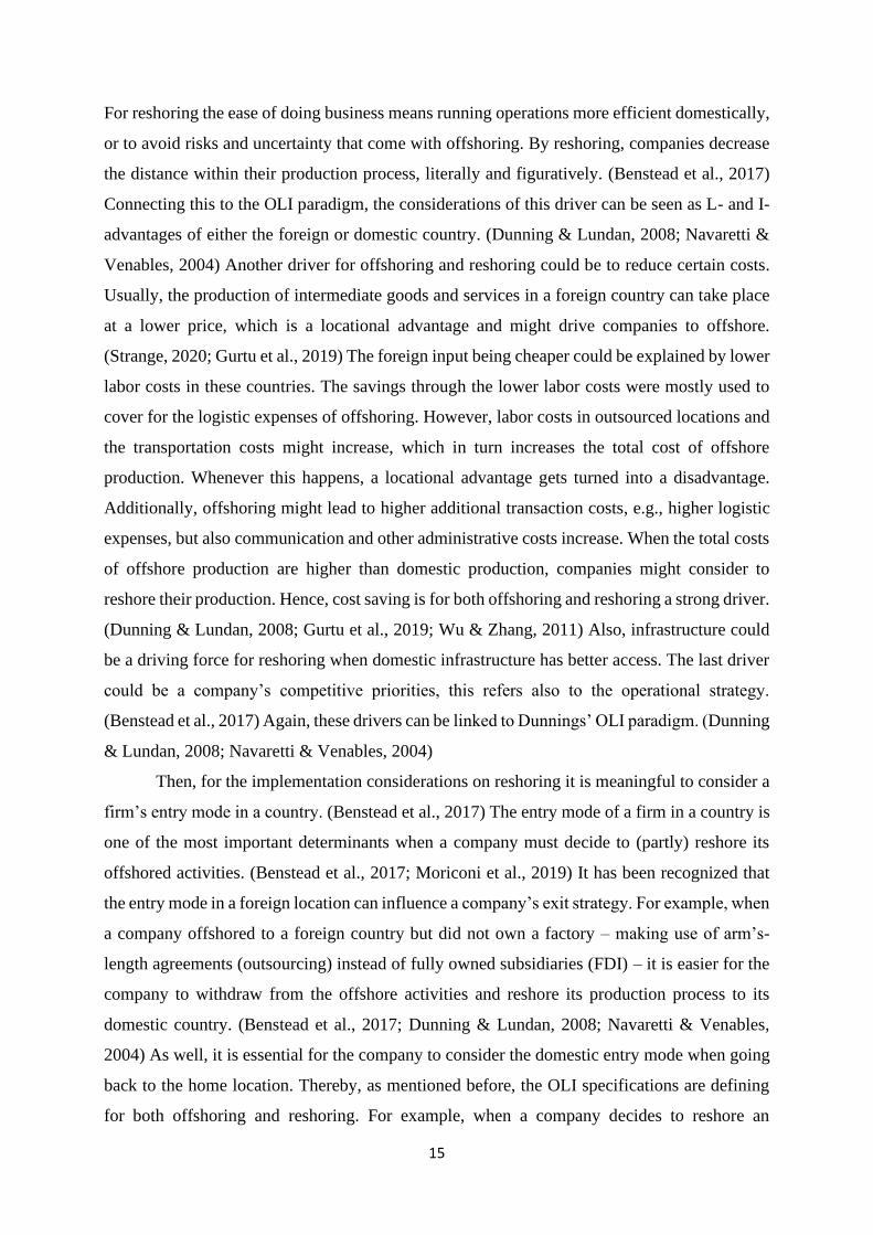
For reshoring the ease of doing business means running operations more efficient domestically,

or to avoid risks and uncertainty that come with offshoring. By reshoring, companies decrease

the distance within their production process, literally and figuratively. (Benstead et al., 2017)

Connecting this to the OLI paradigm, the considerations of this driver can be seen as L- and I-

advantages of either the foreign or domestic country. (Dunning & Lundan, 2008; Navaretti &

Venables, 2004) Another driver for offshoring and reshoring could be to reduce certain costs.

Usually, the production of intermediate goods and services in a foreign country can take place

at a lower price, which is a locational advantage and might drive companies to offshore.

(Strange, 2020; Gurtu et al., 2019) The foreign input being cheaper could be explained by lower

labor costs in these countries. The savings through the lower labor costs were mostly used to

cover for the logistic expenses of offshoring. However, labor costs in outsourced locations and

the transportation costs might increase, which in turn increases the total cost of offshore

production. Whenever this happens, a locational advantage gets turned into a disadvantage.

Additionally, offshoring might lead to higher additional transaction costs, e.g., higher logistic

expenses, but also communication and other administrative costs increase. When the total costs

of offshore production are higher than domestic production, companies might consider to

reshore their production. Hence, cost saving is for both offshoring and reshoring a strong driver.

(Dunning & Lundan, 2008; Gurtu et al., 2019; Wu & Zhang, 2011) Also, infrastructure could

be a driving force for reshoring when domestic infrastructure has better access. The last driver

could be a company’s competitive priorities, this refers also to the operational strategy.

(Benstead et al., 2017) Again, these drivers can be linked to Dunnings’ OLI paradigm. (Dunning

& Lundan, 2008; Navaretti & Venables, 2004)

Then, for the implementation considerations on reshoring it is meaningful to consider a

firm’s entry mode in a country. (Benstead et al., 2017) The entry mode of a firm in a country is

one of the most important determinants when a company must decide to (partly) reshore its

offshored activities. (Benstead et al., 2017; Moriconi et al., 2019) It has been recognized that

the entry mode in a foreign location can influence a company’s exit strategy. For example, when

a company offshored to a foreign country but did not own a factory – making use of arm’s-

length agreements (outsourcing) instead of fully owned subsidiaries (FDI) – it is easier for the

company to withdraw from the offshore activities and reshore its production process to its

domestic country. (Benstead et al., 2017; Dunning & Lundan, 2008; Navaretti & Venables,

2004) As well, it is essential for the company to consider the domestic entry mode when going

back to the home location. Thereby, as mentioned before, the OLI specifications are defining

for both offshoring and reshoring. For example, when a company decides to reshore an

16

offshored production process it might consider a change in its modality choice going from

outsourcing to insourcing, in other words the company decides to internalize its activities (I).

(Benstead et al., 2017; Dunning & Lundan, 2008) Hence, the way of ownership might change

when the location changes and vice versa. Besides, it is acknowledged that reshoring does not

have to contain a company’s whole offshored production process, reshoring can also take place

partially, leaving a part of the offshored production offshore. (Benstead et al., 2017) When a

company does consider (partial) reshoring it should take into account the possible barriers of

gaining access to finance and labor in its domestic country. These barriers could be a result of

the previously made choice to offshore production. The domestic country could have adapted

to the situation of offshored production or was never even in possession of the necessary

finance/labor. Possible ways to overcome these barriers are in-house training, and strong

relationships and information sharing with suppliers. (Benstead et al., 2017)

In addition, whether drivers lead a company to offshore/reshore and the way of

implementing the offshore/reshore decision is affected by contingency factors, as can be seen

in Figure 3. In other words, contingency factors explain indirect influences within the process

of offshoring/reshoring. (Benstead et al., 2017) In additon, these contingency factors can be

linked to one of the specifications of Dunnings’ OLI paradigm (2008). Benstead et al. (2017)

have acknowledged the following eleven contingency factors. First, the size of the organization

could have an influence on the decision making on reshoring. Large organizations are found to

be more active in reshoring, which is explained by the fact that in the first place large

organizations are more active in offshoring. What’s more is that when SMEs do reshore, they

do it earlier than large organizations because of unwillingness or unability to face difficulties

that come with offshoring. (Benstead et al., 2017; Wu & Zhang, 2011) Then, the decision

making on internalizing or outsourcing, Dunnings’ I, is the second contingency factor. This

factor could influence reshoring drivers in terms of their weight, and the time and way reshoring

should take place. Following, reshoring drivers can also be influenced by government policy as

governments can use their policies to make reshoring more attractive and feasible for

companies. (Benstead et al., 2017) Yet, this can similarly be applied on offshoring as foreign

governments can also use their policies to attract companies. In addition, when a company

considers offshoring or reshoring its production, the cost of entry is also of great influence as

this is the fixed cost of the production activities. A country’s cost of entry gets affected by its

legislation, policies, and regulations. While for a company to offshore its production, low cost

of entry in the foreign country would be desirable, for reshoring it would be desirable for the

domestic country to have low entry cost. (Moriconi et al., 2019) Moriconi et al. (2019) studied

17

the effect of institutional fixed costs and immigration networks on offshoring, as these are part

of the entry costs. They found that offshoring is negatively affected by institutional fixed costs

as they are positively related to the entry costs of a country. On the contrary, immigrant

networks are positive related to offshoring. The idea behind this is that a company may draw

on the connections and knowledge of its foreign workers which will reduce the cost of entry of

the country of origin of the workers. (Moriconi et al., 2019) Connecting the attractiveness and

entry cost of a country to the OLI paradigm, it is to say that it can be seen as L-specifications.

(Dunning & Lundan, 2008) Then, the fourth contingency factor mentioned is capital

intensiveness. Low capital intensive productions are seen to be more often offshored than high

capital intensive productions. This is explained by the reasoning of low capital intensive

productions being involved with high labor content, which is more likely to take place offshore,

in lower wage countries. (Benstead et al., 2017; Wu & Zhang, 2011) In addition to the in-house

decision making of companies, actions of competitors may also influence the decision making

of an organization. Therefore, bandwagon effects (competitive pressure) are also seen as a

contingency factor. Thereafter, the following contingency factors are based on properties of the

produced good: market segment, price point, bulkiness of the product and customised products.

Another factor could be the management’s perception of cost, which refers to misjudgements

in the offshoring decision making process which might lead to a company to decide on

reshoring. Lastly, emotional factors might have an effect on the influence of drivers on the

decision to offshore/reshore. For example, fear of risks (risk aversion) might increase the

influence the weight on reshoring drivers. (Benstead et al., 2017)

18

Figure 3. Reshoring (Offshoring Reversed)

Source: Benstead et al., 2017, p. 91, Figure 2.

2.2 Propositions

Before, companies would offshore their productions based on location advantages (L) and

drivers such as cost saving through lower labor costs in foreign country; expanding capacities;

access to markets and talent pool; reducing unsystematic risk by GVCs; etc. Companies were

also familiar with the disadvantages of offshoring, such as higher transaction costs. (Strange,

2020; Gurtu et al., 2019) However, time has changed and based on the information provided in

previous sections, the pandemic is a new phenomenon, affecting the whole world. Therefore, it

comes with a lot of uncertainty and enlarges the risks of international trade and GVCs.

Moreover, borders have been closed, and companies were put to a stop as a measure against the

spread of the pandemic. This resulted in shocks in the supply and demand chains which directly

affects GVCs. (Barbieri et al., 2020; Shingal & Agarwal, 2020) Furthermore, these shocks in

supply chains have pointed out the need for economic self-sufficiency among many economies.

But also the need for better strategies to cope with global risks that come with, or are enlarged

by, such crises. One of the reactions of countries has been the establishment of more trade

19

policy interventions, which goes at the cost of international trade and affects GVCs. (Seric et

al., 2021)

Reflecting this on the drivers for offshoring and reshoring, the pandemic might cause

some changes among companies’ earlier decisions on their production process. The increase in

uncertainty and risks, and the measures taken as a result of the pandemic could be a reason for

companies to (partly) reshore their operations. Based on the drivers of reshoring, reshoring

would give companies more certainty and lowers the risks. In addition, transactions costs of

offshoring, e.g., transportation costs, have been enlarged as a result of the measures taken

against the spread of the virus. Therefore, through (partly) reshoring operations, a company can

also save costs as a result of lower transportation costs. (Benstead et al., 2017) Hence, when

production processes are fully reshored it will decrease the amount of GVCs and when partly

reshored, it will decrease the length of GVCs.

Furthermore, within this study is has become clear that understanding the effect of the

pandemic on GVCs in the long run is of great importance. Therefore, the main aim of this study

is to examine the effect of COVID-19 on Global Value Chains (GVCs). Hence, this study will

give answer to the following research question: What will be the effect of COVID-19 on Global

Value Chains? From the previous sections, it can be summarized that it is important to

understand a company’s motives for offshoring and reshoring as those have a direct effect on

GVCs. Therefore, this study is going to examine the effect of similar crises like the pandemic

on the amount and length of GVCs. Based on the literature, it would be plausible to think that

companies would (partly) reshore their production activities as a reaction on crises such as the

pandemic which would affect the amount and length of GVCs. For example, the costs of doing

business on an international level might increase as a result of the pandemic, which would give

companies a reason to partly or wholly reshore their operations. This would shorten or decrease

the amount of GVCs. It is for that reason, that the propositions of this study relate to the decision

making on reshoring offshored productions. The first proposition therefore relates to the amount

of GVCs. The second proposition relates to the length of GVCs, to see if the length of GVCs is

affected by the crisis. Hence, the following propositions are suggested:

Proposition 1: COVID-19 is expected to have a negative effect on the importance of GVCs in

the world.

Proposition 2: COVID-19 is expected to have a negative effect on the length of GVCs.

20

III. Data and Method

This chapter sets out the collection of data and the empirical strategy for this study. This

empirical strategy is built upon the key elements of the theoretical framework set out in the

previous chapter. Furthermore, it elaborates on the methods used within the quantitative

research to examine the propositions made in chapter II.

COVID-19 seems to influence Global Value Chains. However, because the pandemic

is such a new phenomenon it is uncertain what the long-term effect of the pandemic will be on

GVCs. The recency of the pandemic ensures that the propositions made in Section 2.2 cannot

be examined directly. Therefore, looking back at recently happened disasters with similar

properties as the current pandemic that affected GVCs, might help predicting the effect of

COVID-19 on the importance of GVCs and the length of GVCs.

First, COVID-19 is compared to two epidemics, named SARS and MERS, which

happened over the last two decades and are most representative of the pandemic. The epidemics

and the pandemic share similarities in nature, in other words they form a similar type of disaster.

All three the disasters – SARS, MERS and COVID-19 – carry the same properties as containing

symptoms like the flu, and their quick spread originated from an epicenter. (Shingal & Agarwal,

2020) As for MERS the contagion is in the first place from dromedary camels to human and

does not as much occur from human to human like SARS, it is the spread of SARS that is most

comparable to the spread of COVID-19. (Pietrasik, 2021; Frost, 2021) In addition, the

disruption of value chains has been similar for the previous epidemics and the current pandemic.

On the other hand, the main difference between COVID-19 and previous epidemics lays in the

fact that for the latter two ‘only’ a few countries were hit by the epidemics while COVID-19 is

a pandemic and therefore affects the whole world. Hence, the epidemics are not fully

representative for the pandemic as they fall short in their comprehensive effect. (Shingal &

Agarwal, 2020) Nonetheless, this study tests for the effect of the epidemics on the importance

of GVCs and the length of GVCs.

Thereafter, a comparison is made between the pandemic and the 2008 financial crisis

based on their comprehensive effects. Both crises managed to hit economies worldwide.

(Danielsson et al., 2020) Yet the difference between the financial implications that came with

the pandemic and the financial crisis of 2008 is the time in which it caused a globally felt effect.

Whereas ‘normal’ financial crises like the crisis of 2008 will spread to other countries in a

certain amount of time after it started in one or two countries, the COVID-19 crisis spread fast,

all advanced economies were hit at the same time by the underlying shock. (Baldwin, 2020) In

21

addition, these two crises also differ because of their remedies. As mentioned, the pandemic

caused both a health and an economic crisis. Policy responses designed to constrain the spread

of the virus exacerbate the negative impact on the economy, and vice versa. Therefore, the

potential remedy for the pandemic is much more difficult to conceive and harder to match the

underlying problem than for the financial crisis of 2008. (Strange, 2020) Nonetheless, because

of the similarities in comprehesiveness and because this study is considering the effect of a

crisis on GVCs, which is a more economic effect, the comparison made with the financial crisis

is considered more valid than the epidemics.

3.1 Data

As the pandemic is recent, it is not possible to get long-term data on the effect of COVID-19

on GVCs. Hence, this study uses historical data on previous disasters in order to do the

quantitative research and to examine the propositions made on the effect of the pandemic on

GVCs to determine the long-run effects. To test for the importance of GVCs, this study

determines if previously happened disasters have had a significant effect on the total value of

GVCs. In addition, to test for the effect of previous crises on the length of GVCs, this study

examines the effect of the crises on the key GVC indicators. The key GVC indicators include

Domestic Value Added, Foreign Value Added and Indirect Value Added. A more

comprehensive explanation on the indicators is given below. To measure the effect of the

pandemic on the length of GVCs, this study will examine if the previous crises have had a

significant effect on the Foreign Value Added. As a robustness check, this study looks at the

effect of the crises on the other two indicators to see if this is in line with the results of the study

done on Foreign Value Added. The GVC indicators are not a perfect measure of the length of

GVCs, as they indicate the value of the indicator, which gives an indication of the length of

GVCs, but not the exact number of border crossings during a production process. For example,

when the value of an indicator increases, it means that the importance of the indicator has

increased relatively, which is expected to influence the length of GVCs.

The data on GVCs and the key indicators are on country level and collected from the

UNCTAD-Eora Global Value Chain Database. This database covers 189 countries, and the

remaining countries are included within a region called ‘the rest of the world’. The database

covers a data-frame from 1990 to 2018, of which the timeframe from 1999 to 2018 is used for

this study as it is related to the crises studied. Moreover, the database includes GVC indicators

based on value added (VA). (UNCTAD-Eora Global Value Chain Database, 2019; Casella et

al., 2019) When refering to value added (VA) the following definition is used: “Value-added

22

trade is the value generated by one country but absorbed by another country, while the domestic

content of exports depends only on where value is produced, not where and how that value is

used.” (Koopman et al., 2010)

This study makes use of the following key GVC indicators:

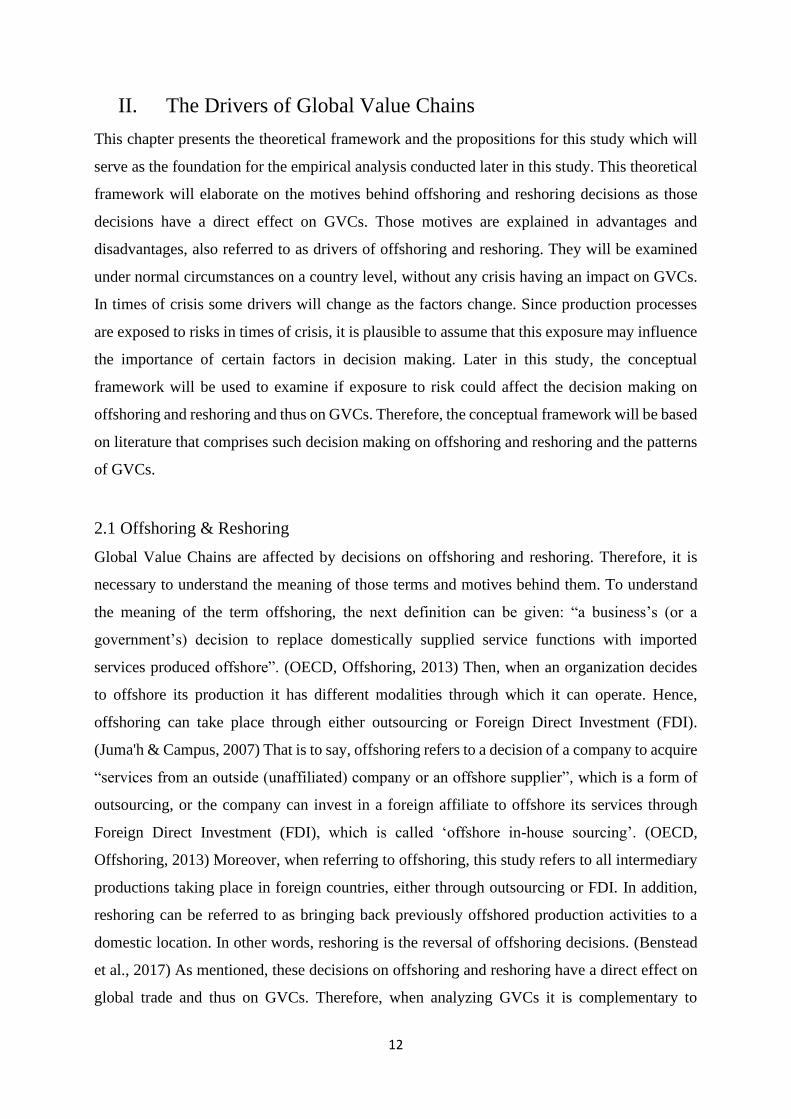
- Domestic Value Added (DVA), which refers to the value added by domestic

industries/companies within a country’s exports. In other words, the inter-sector flows

are domestic. For example, Figure 4 shows country A has an exports’ value of 170, from

which 45 is added by country A, the domestic country. Therefore, the Domestic Value

Added (DVA) of country A is 45.

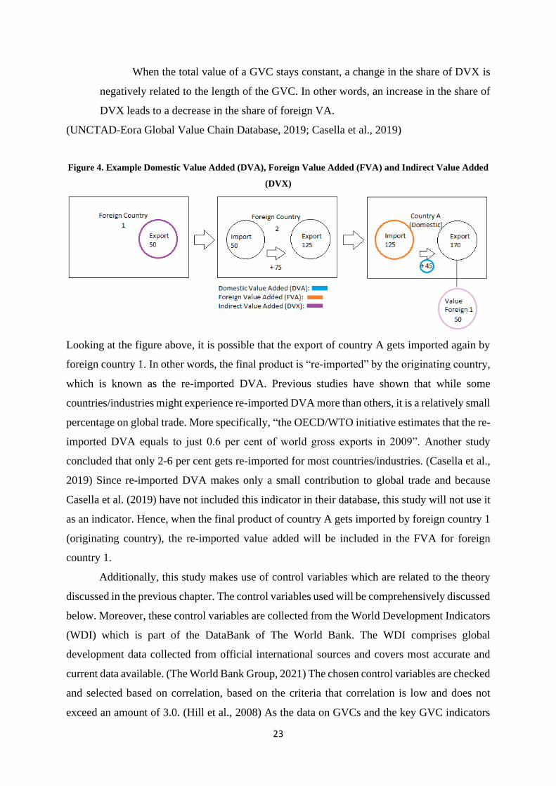
When the total value of a GVC stays constant, a change in the share of DVA is

assumed to be negatively related to the length of the GVC. In other words, an increase

in the share of DVA leads to a decrease in the share of foreign VA. Moreover, when the

share of foreign VA decreases it means that either the VA in a foreign country has

decreased or the number of foreign countries involved in the GVC has decreased.

Therefore, this study assumes that when the share of DVA increases, it will decrease

the length of the GVC.

- Foreign Value Added (FVA), which refers to the value added by foreign

industries/companies within a country’s exports. In other words, country A requires

inputs from other countries to produce its output. A part of this output generated by

country A will be exported. Therefore, through their inputs, other countries also add

value to the output of country A. For example, in Figure 4, country A has an export

value of 170 of which 125 was imported from foreign countries, which is seen as the

Foreign Value Added.

When the total value of a GVC stays constant, a change in the share of FVA is

assumed to be positively related to the length of the GVC. In other words, an increase

in the share of FVA leads to an increase in the share of foreign VA. Moreover, when

the share of foreign VA increases it means that either the VA in a foreign country or the

number of foreign countries involved in the GVC has increased. Therefore, this study

assumes that when the share of FVA increases, it will increase the length of the GVC.

- Indirect Value Added (DVX), which refers to the value added by domestic

industries/companies within exports of other countries. In other words, looking at Figure

4, DVX gives the share of the domestic value added produced by foreign country 1 that

turns into an intermediate input in the value added of exports produced by the other

countries.

23

When the total value of a GVC stays constant, a change in the share of DVX is

negatively related to the length of the GVC. In other words, an increase in the share of

DVX leads to a decrease in the share of foreign VA.

(UNCTAD-Eora Global Value Chain Database, 2019; Casella et al., 2019)

Figure 4. Example Domestic Value Added (DVA), Foreign Value Added (FVA) and Indirect Value Added

(DVX)

Looking at the figure above, it is possible that the export of country A gets imported again by

foreign country 1. In other words, the final product is “re-imported” by the originating country,

which is known as the re-imported DVA. Previous studies have shown that while some

countries/industries might experience re-imported DVA more than others, it is a relatively small

percentage on global trade. More specifically, “the OECD/WTO initiative estimates that the re-

imported DVA equals to just 0.6 per cent of world gross exports in 2009”. Another study

concluded that only 2-6 per cent gets re-imported for most countries/industries. (Casella et al.,

2019) Since re-imported DVA makes only a small contribution to global trade and because

Casella et al. (2019) have not included this indicator in their database, this study will not use it

as an indicator. Hence, when the final product of country A gets imported by foreign country 1

(originating country), the re-imported value added will be included in the FVA for foreign

country 1.

Additionally, this study makes use of control variables which are related to the theory

discussed in the previous chapter. The control variables used will be comprehensively discussed

below. Moreover, these control variables are collected from the World Development Indicators

(WDI) which is part of the DataBank of The World Bank. The WDI comprises global

development data collected from official international sources and covers most accurate and

current data available. (The World Bank Group, 2021) The chosen control variables are checked

and selected based on correlation, based on the criteria that correlation is low and does not

exceed an amount of 3.0. (Hill et al., 2008) As the data on GVCs and the key GVC indicators

24

serve as the dependent variables, the collection of the data on the control variable has the same

properties. The collected data is also on country level and covers the same countries and the

timeframe used is from 1999 to 2018.

This study makes use of the following control variables:

- GDP per Capita (current US$) (GDP): refers to the value added that is created within

an economy (country) in current US dollars. Since it is per capita it means that the GDP

has been divided by midyear population and thus it gives a good perspective when

comparing to other economies. This variable has been chosen as it gives a good

impression on the wealth within an economy. (The World Bank Group, 2021)

- Compulsory Education, duration (years) (CE): refers to the legally obliged number of

years a child must attend school within a country. Compulsory education gives an

impression on a country’s believe in the development of children, but it also gives an

impression on child labor. (The World Bank Group, 2021) When compulsory education

is low, it can be assumed that children must work from an early age, leading to lower

wages and higher labor content. This relates to the contingency factor capital

attractiveness, discussed in Section 2.1. As mentioned above, it is common for low

capital-intensive productions to involve high labor content, which is attractive for

offshoring. (Benstead et al., 2017; Wu & Zhang, 2011) Therefore, compulsory

education is expected to have a positive relationship with GVCs. Furthermore, it is also

related to the contingency factor government policy since the government has a direct

influence on the amount of compulsory education. Hence, this indicator has been chosen

as a control variable as it is related to the literature and it is expected to influence GVCs

and its key indicators.

- School Enrollment Secondary Grade (SESG): refers to the gross enrollment ratio, it

gives the percentage of how many people have been enrolled to secondary education.

The aim of secondary education is to lay foundations for human development and

lifelong learning, and it is more subject- or skill-oriented than the primary education.

Hence, it gives an impression on the level of the subject- or skill-orientation of a

country’s population. (The World Bank Group, 2021) This indicator is also related to

the contingency factor capital attractiveness and besides it influences the driver

competitive priorities. When the gross enrollment ratio on secondary education

increases it could be assumed that it will result in higher capital-intensive work.

Thereby, it will also stimulate innovation as people become more skilled and educated

25

which increases competitive priories. Again, this influences GVCs and its key indicators

which is the reason why this indicator is part of the control variables within this study.

- Cost of Business Start-up (CBSU): refers to the cost of registering a business as a

percentage of the gross national income (GNI) per capita. (The World Bank Group,

2021) This indicator is also expected to have a negative relationship with the

attractiveness of a country to start a business. As this influence’s offshoring/reshoring

decision making and therefore on GVCs, this indicator is used as a control variable.

- Taxes on International Trade (TIT): refers to all taxes on international trade as a

percentage of the government’s revenue. Included are export duties, import duties,

profits of export/import monopolies, exchange profits, and exchange taxes. (The World

Bank Group, 2021) When taxes on international trade are a high percentage of a

government’s revenue, the country would be unattractive for international trade for both

domestic companies doing business with foreign countries and foreign companies doing

business in the concerning country. Therefore, it is expected to have a negative

relationship with GVCs. Because of its expected influence on GVCs, this study has

taken this indicator as a control variable.

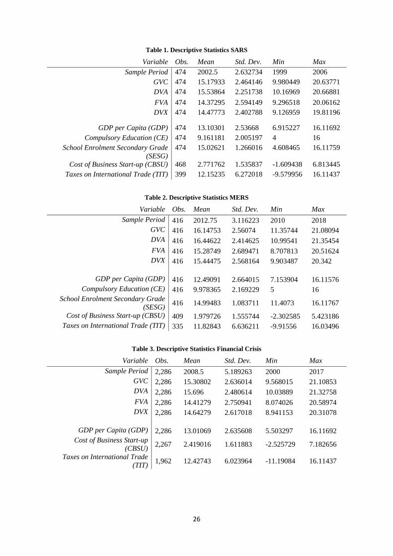
To provide an overview of all variables used and the corresponding data, the descriptive

statistics are discussed in the tables below. As previously mentioned, this study uses data from

the SARS and MERS epidemics, and the 2008 financial crisis to see what effect crises with

similar characteristics to the pandemic have had on GVCs, to make a prediction about the effect

of COVID-19 on GVCs. Since the variables GVC, DVA, FVA, DVX, GDP per Capita, School

Enrollment Secondary Grade, Cost of Business Start-up and Taxes on International Trade were

found to have a skewed right distribution, and thus are not normally distributed, a lognormal

distribution was used. Thereby, the discrepancies in observations for the variables Cost of

Business Start-up and Taxes on International Trade can be explained by the fact that some

countries had a value of zero for the variable and these are not included by Stata. Given that the

crises were each studied separately, the descriptive statistics presented below summarize the

data analyzed separately for each crisis.

26

Table 1. Descriptive Statistics SARS

Variable Obs. Mean Std. Dev. Min Max

Sample Period 474 2002.5 2.632734 1999 2006

GVC 474 15.17933 2.464146 9.980449 20.63771

DVA 474 15.53864 2.251738 10.16969 20.66881

FVA 474 14.37295 2.594149 9.296518 20.06162

DVX 474 14.47773 2.402788 9.126959 19.81196

GDP per Capita (GDP) 474 13.10301 2.53668 6.915227 16.11692

Compulsory Education (CE) 474 9.161181 2.005197 4 16

School Enrolment Secondary Grade

(SESG)

474 15.02621 1.266016 4.608465 16.11759

Cost of Business Start-up (CBSU) 468 2.771762 1.535837 -1.609438 6.813445

Taxes on International Trade (TIT) 399 12.15235 6.272018 -9.579956 16.11437

Table 2. Descriptive Statistics MERS

Variable Obs. Mean Std. Dev. Min Max

Sample Period 416 2012.75 3.116223 2010 2018

GVC 416 16.14753 2.56074 11.35744 21.08094

DVA 416 16.44622 2.414625 10.99541 21.35454

FVA 416 15.28749 2.689471 8.707813 20.51624

DVX 416 15.44475 2.568164 9.903487 20.342

GDP per Capita (GDP) 416 12.49091 2.664015 7.153904 16.11576

Compulsory Education (CE) 416 9.978365 2.169229 5 16

School Enrolment Secondary Grade

(SESG) 416 14.99483 1.083711 11.4073 16.11767

Cost of Business Start-up (CBSU) 409 1.979726 1.555744 -2.302585 5.423186

Taxes on International Trade (TIT) 335 11.82843 6.636211 -9.91556 16.03496

Table 3. Descriptive Statistics Financial Crisis

Variable Obs. Mean Std. Dev. Min Max

Sample Period 2,286 2008.5 5.189263 2000 2017

GVC 2,286 15.30802 2.636014 9.568015 21.10853

DVA 2,286 15.696 2.480614 10.03889 21.32758

FVA 2,286 14.41279 2.750941 8.074026 20.58974

DVX 2,286 14.64279 2.617018 8.941153 20.31078

GDP per Capita (GDP) 2,286 13.01069 2.635608 5.503297 16.11692

Cost of Business Start-up

(CBSU) 2,267 2.419016 1.611883 -2.525729 7.182656

Taxes on International Trade

(TIT) 1,962 12.42743 6.023964 -11.19084 16.11437

27

3.2 Methodology

3.2.1 Method Epidemics SARS and MERS

To test for the effect of the SARS and MERS epidemics on GVCs, this study will examine the

difference between what happened with the GVC indicators during the crises and what would

have happened had the crises not happened. Therefore, this study contains a difference-in-

difference analysis for the quantitative research on the epidemics SARS and MERS. For this

difference-in-difference analysis, the epidemics SARS and MERS are used as treatments. Thus,

when speaking about a treatment, this study refers to the epidemics studied. Consequently, the

difference in differences in observed outcomes between the affected (treated) and non-affected

(non-treated) countries will be compared across periods before and after the epidemics. Besides,

this difference-in-difference analysis, the regression will control for the fact that an observation

of the GVC indicators is from the crises period and whether it belongs to the group of affected

countries. (Abadie, 2005; Bertrand et al., 2004)

The basic specification of the difference-in-difference model is as follows:

𝛿𝑖𝑡 = 𝛼1 + 𝛼2𝐷𝑇 + 𝛼3𝐷𝑌 + 𝛼4𝐷𝑇𝑌 + 𝛼5𝐺𝐷𝑃 + 𝛼6𝐶𝐸 + 𝛼7𝑆𝐸𝑆𝐺 + 𝛼8𝐶𝐵𝑆𝑈 + 𝛼9𝑇𝐼𝑇 + 휀𝑖𝑡

Where 𝛿𝑖𝑡 is the dependent variable, so either GVC or one of the key indicators of GVCs,

depending on the proposition examined. Moreover, the parameter i represents the group of

countries studied and t represents the time period of the study. The residual is given by 휀𝑖𝑡.

Within this model the variable 𝐷𝑇 represents a dummy variable of the treatment period, for

which the dummy variable has a value of zero for the period before the treatment (epidemic)

and a value of one for the period after the treatment. This study has taken one to three years for

the periods before and after the treatment, depending on the availability of data. For the study

on SARS, 𝐷𝑇 equals zero for the period 1999-2001 (before), and one for the period 2004-2006

(after). For the study on MERS, 𝐷𝑇 equals zero for the period 2010-2012, the period before the

treatment, and one for 2018, the period after the treatment. The period after the treatment for

MERS is only one year because there is no more recent data available on GVCs and the key

indicators. The variable 𝐷𝑌 represents a dummy variable including the treatment group and the

control group. In other words, 𝐷𝑌 has a value of zero for the non-affected countries (control

group) and a value of one for the affected (treatment group) countries. For SARS, the treatment

group consists of China, Canada, Singapore and Vietnam as those countries were affected by

the epidemic. The control group encompasses 75 countries, which can be explained by the

28

number of countries included in the UNCTAD-Eora Global Value Chain Database that had a

value above zero for minus missing data among the control variables. A more detailed

explanation on how this study has handled with missing data will be provided below. For

MERS, the treatment group consists of Saudi Arabia, United Arab Emirates, and the Republic

of Korea. Hence, the control group encompasses 101 countries, which again can be explained

by the number of countries included in the UNCTAD-Eora Global Value Chain Database that

had a value above zero for minus missing data among the control variables. Then, variable 𝐷𝑇𝑌

is a dummy variable controlling for the fact that an observation belongs to the group of treated

and whether it is from the treatment period. Therefore, variable 𝐷𝑇𝑌 is also called the interaction

term and captures the difference in differences. For the study on SARS this means that the

interaction term can only have a value of one if the results are from the period 2004-2006 and

the country was affected by the epidemic. For the study on MERS this means that the interaction

term can only have a value of one if the results are from 2018 and the country was affected by

the epidemic. (University of Copenhagen;, 2019) The control variables for this analysis are

GDP per capita (GDP), compulsory education duration (CE), School enrollment secondary

grade (SESG), Cost of business start-up procedures (CBSU), and Taxes on international trade

(TIT). To correct for missing data among the control variables, this study used a dummy

variable adjustment, replacing the missing data with the average value of the variable in

question for the country in question when possible to avoid too much data loss. If it was not

possible to subtract the average value of a variable for a specific country, the country was not

included in the analysis. (Hill et al., 2008)

Moreover, the assumptions of the difference-in-difference equal the assumptions of the

OLS model. An important assumption is that data is normally distributed. However, as

mentioned before, the majority of the variables happened to have a “skewed right” distribution

which means that they have long right tail. Therefore, a lognormal distribution is used for the

variables GVC, DVA, FVA, DVX, GDP per Capita, School Enrollment Secondary Grade, Cost

of Business Start-up and Taxes on International Trade. In addition, there is, among other things,

the assumption that there is no correlation between the explanatory variable, the epidemic

(treatment), and the residual. A general issue is that obtaining the treatment and the outcome

variable are in reality often related. Moreover, the explanatory variable and the residual would

then be correlated and there would be nonrandomness which leads to a biased estamation. This

would normally result in using an Instrumental Variable. (Hill et al., 2008) However, for this

study the assumption on having no correlation between the explanatory variable and the residual

can be maintained. Since epidemics are a result of infectious diseases it is important to

29

understand the occurrence and spread of such infectious diseases as this will show that there is

no correlation between the explanatory variable and the residual. According to a report on

epidemics and infectious diseases, the occurance of infectious diseases is a ‘blind’ process

which results from constant accidental changes in genetics of germs, bacteria and viruses.

Therefore, it can be stated that the outbreak of an infectious disaese, and thus an epidemic, is at

random. In addtion, the transmission of infectious diseases differs per disease.

(Vandenbroucke-Grauls et al., 2021) For SARS the transmission was meanly from human to

human and for MERS it was meanly from dromedary camels to human and another human

could then be inderctly infected. However, there is no clear reason why some countries suffered

from an epidemic caused by the virus and others with similar characteristics did not or less.

(Pietrasik, 2021; Frost, 2021) Therefore, it also applies to the spread of the epidemic that it

happened at random. Hence, there is no correlation between the acquisition of the treatment

(epidemic) and the outcome variable and thus difference-in-difference analysis is sufficient.

(Hill et al., 2008)

To conclude, to measure the effect of the epidemics on the importance and length of the

GVCs, a difference-in-difference analysis is performed in this study. Having China in the

treatment group for the SARS epidemic could give a biased effect, since China is a very large

country relative to the other affected countries and it was also economically emerging at the

time. In order to verify whether the presence of China in the treatment group had an effect on

the results, the analysis was conducted again with China excluded from the treatment group. In

addition, for the MERS epidemic, China was not included in the treatment group. In order to

determine whether the absence of China in the treatment group influenced the results, the

analysis was conducted again with China in the treatment group. In addition, the countries

included in the treatment group for the main analysis of the impact of the MERS epidemic were

those that were hardest hit. However, the spread of the virus has also reached many other

countries, including some Western countries in the E.U. and the U.S. (Middle East Respiratory

Syndrome (MERS), 2019) Therefore, another robustness check was conducted to measure

whether the results differ when all affected countries are included in the treatment group,

compared to the first choice of treatment group. This study also examined whether the impact

of the MERS epidemic would have been different if only the affected Western countries were

included in the treatment group compared to the first choice of treatment group.

30

3.2.2 Method Global Financial Crisis

For the global financial crisis this study will make use of Panel Data Analysis to study the effect

of the financial crisis on GVCs. As the financial crisis hit most of the world panel data is

preferred over the difference-in-difference analysis. With the use of panel data, it is possible to

examine data from different countries across time, it provides a better indication of a causal

relationship. For panel data, the following formula is used:

𝑌𝑖𝑡 = 𝛽0 + 𝛽1𝑋𝑖𝑡 + 𝑢𝑖𝑡 + 𝑎𝑖 + 𝜇𝑡 + 𝐺𝐷𝑃 + 𝐶𝐵𝑆𝑈 + 𝑇𝐼𝑇

Where, Y is the dependent variable, so either GVC or one of the key indicators of GVCs,

depending on the proposition examined. The explanatory variable, the financial crisis, is given

by X. Moreover, the parameter i stands for the economic entity, the countries in this study, and

t stands for the time scale. (Hill et al., 2008) The dataset used for this analysis covers 127

countries, which again can be explained by the number of countries included in the UNCTAD-

Eora Global Value Chain Database that had a value above zero for minus missing data among

the control variables. For this study the time frame contains the years 2000 to 2017, based on

the literature of World Bank & World Trade Organization (2019), discussed in chapter I.

Officially the financial crisis took place in 2008 and 2009, which is used in this study. For the

period after the crisis, this study took 2010 to 2017 as the financial crisis has had a significant

aftermath in the post-crisis years. (World Bank & World Trade Organization, 2019) Moreover,

𝑢𝑖𝑡 is the error term and 𝑎𝑖 encompasses the economic entity specific variation which is a

variation that does not change over time. Additionally, 𝜇𝑡 is the time variation, it gives the

variation for all economic entities between years, and these are simultaneously affected. In other

words, 𝑎𝑖 encompasses the country fixed effects and 𝜇𝑡 the time fixed effects. (Hill et al., 2008)

The control variables for this analysis that are used are GDP per Capita (GDP), Cost of Business

Start-up (CBSU), and Taxes on International Trade (TIT). Once more, to correct for missing

data among the control variables, this study used a dummy variable adjustment, replacing the

missing data with the average value of the variable in question for the country in question when

possible. In case this was not possible, the related data was not included in the analysis.

Additionally, for panel data a common method is to use pooled regression. For this

regression, some strong assumptions are made such as the assumption that the behavior of

entities is similar through the years. These strong assumptions are for most studies somewhat

unrealistic and one could question if the pooled regression is the right way to analyze the panel

data. To test for the necessity to use another method than the pooled regression a Chow Test

31

could be performed to test for differences between economic entities. As it already can be

concluded that the economic entities (the countries) in this study differ from one another, it is

not necessary to perform the Chow Test. Furthermore, these differences between countries

might cause the countries to have different intercepts and coefficients. To solve for the different

intercepts, one could use the Fixed Effects (FE) model. By removing 𝑎𝑖, FE removes the

economic entity specific variation. Then, by adding dummies FE corrects for the time invariant

effects. Moreover, unique individual characteristics of entities are captured over time.

Moreover, the FE model is seen as a very strong model, however, it also has some restrictions

to it. It is not possible to measure variables which do not change over time. Additionally, the

dummies used in a regression capture all characteristics that are stable. Hence, when using the

FE model, it is not possible to use variation for estimating effects of variables that vary between

economic entities. Concluding, the FE model only measures variables that change over time.

(Hill et al., 2008)

To overcome the restrictions of the FE model, the Random Effects (RE) could be used

for panel data. The RE model adds a random part which allows the model to include variables

that are constant over time. However, a disadvantage of the RE model would be that correlation

between the explanatory variable and the error term could lead to an overestimation of the

coefficients. Therefore, correlation between the explanatory variable and the error term would

lead to biased results. To test for the reliance of the RE model, and thus for correlation between

the explanatory variables and the error term, one could use the Hausman Test. If the test

determines that there is no correlation, one could use the RE model. Otherwise, in case of

correlation, and thus the Hausman test p-value is below 0.05, one should use the FE model.

(Hill et al., 2008)

What’s more, to measure the effect of the financial crisis on the importance and length

of the GVCs, a FE and RE analyses is performed in this study. As the financial crisis has had a

significant aftermath in the post-crisis years, this study has done robustness checks to see if the

aftermath might have had an effect on the results of the analyses done. Therefore, the analyses

was conducted again with a change in crisis period. First, the original crisis period was extended

to include the aftermath period 2012-2016 to see if this would give another result than the

original analysis. Thereafter, another analysis was conducted in which the crisis period included

only the aftermath period 2012-2016 to see what the effect of the aftermath has been on the

importance and length of GVCs.

32

IV. Empirical Results

This chapter sets out the empirical results of this study. Primarily, by means of the difference-

in-difference method, this study has estimated the effect of the epidemic caused by epidemics

SARS and MERS on the importance of GVCs in the world and on the length of GVCs. The

results of these difference-in-difference analyses are shown and discussed in Sections 4.1 and

4.2. Thereafter, by means of the FE model, this study has estimated the effects caused by the

financial crisis of which the results are shown and discussed in Section 4.3.

4.1 Results SARS

This section will discuss the results of the difference-in-difference analyses done on the effect

of SARS, shown in Table 4 (below). According to this statistical analysis done on the effect of

SARS on GVCs, it can be concluded that the sample period does have a significant positive

effect. This means that the total value of GVCs is higher for the years 2004 to 2006, the period

after the SARS epidemic. In other words, it means that the total value of GVCs has increased

over time, but it does not look at the difference between affected and non-affected countries.

Nonetheless, the variable Affected Countries, so whether a country was affected by the

epidemic in the years 2002 and 2003, appears to have no significant effect. In addition, when

looking at the interaction term (years&affected) it also shows there is no significant effect. This

means that the data on GVCs for Affected Countries in the years 2004 to 2006 (after the

epidemic) does not significantly differ compared to the period before the epidemic or compared

to the countries that were not affected by the epidemic. It is interesting to see that the interaction

term shows no significant effect as this is in line with the expectations based on previous

research done by Simola (2021) and Shingal and Argarwal (2020), that the epidemic had no

significant long-term effect on the total value of GVCs. When looking at the control variables,

it appears that the GDP per capita has a significant negative effect on GVCs. In addition, the

control variable compulsory education produces a significant positive result, which is not in

line with the expectations expressed in the data description section. Nonetheless, the significant

negative results on the control variables cost of business and taxes on international trade are in

line with the expectations.

Furthermore, to measure the effect of the epidemic on the length of GVCs this study has

done the difference-in-difference analysis on FVA, and in addition the effect on DVA and DVX

as a robustness check. The results of the analysis done on FVA show similar outcomes as the

analysis done on GVC. First, the sample period does have a significant positive effect. Here,

33

however, the variable Affected Countries appears to have a significant positive effect.

Therefore, the countries affected by the SARS epidemic have experienced an increase in the

FVA and thus on the length of GVCs. However, to see if the epidemic had a significant effect

on the total amount of GVCs it is important to look at the interaction term. Moreover, the

interaction term (years&affected), again, does not give a significant effect. Once more, it is

interesting to see that these results show no significant effect, which means that the SARS

epidemic had no significant long-term effect on the length of GVCs. Furthermore, the results

of the control variables are in line with the analysis done above. The control variable

compulsory education has a significant positive effect on FVA, while the control variables GDP

per capita, cost of business and taxes on international trade have a significant negative effect.

The analyses done on DVA and DVX as robustness checks have confirmed the discussed results

from the analysis done on FVA. According to the results of the analyses on the key GVC

indicators the length of GVCs has increased over time but there was no significant long-term

effect of the SARS epidemic.

Moreover, among the affected countries is China, which is very large relative to the

other affected countries and was also emerging economically at the time. To see if having China

in the treatment group has influenced the results the analysis has been performed again with

China left out of the treatment group. However, removing China from the treatment group had

no effect at all on the analysis, so no effect on Table 4 below. So contrary to expectations, the

fact that China is part of the treatment group did not give biased results.

In conclusion, based on the difference-in-difference analysis done to measure the effect

of the SARS epidemic on the importance of GVCs and the length of GVCs, this study found

that there was no significant long-term effect of SARS on the importance or the length of GVCs.

Therefore, these findings contradict the propositions made, as the crisis was expected to have a

negative impact on the importance and length of GVCs. Nonetheless, these findings are

consistent with the expectation of Simola (2021) and, Shingal and Argarwal (2020), that GVCs

are well founded and unlikely to change as a result of a crisis.

34

Table 4. Difference-in-Difference Analysis SARS

SARS GVC FVA DVA DVX

Sample Period (𝐷𝑇) .4383266*

(2.43)

.4154697*

(2.30)

0.3730464*

(2.16)

.4629809*

(2.52)

Affected Countries (𝐷𝑌) 1.982275

(1.85)

2.386822*

(2.22)

2.069536*

(2.02)

1.356769

(1.24)

GDP per Capita (GDP) -.0945532*

(-2.20)

-.1115188**

(-2.58)

-.1012343*

(-2.45)

-.0830833

(-1.89)

Compulsory Education

(CE)

.1639038***

(3.58)

.1930259***

(4.20)

.1403963***

(3.20)

.1432206**

(3.07)

School Enrolment

Secondary Grade (SESG)

-.0484267

(-0.57)

-.0040978

(-0.05)

-.0784382

(-0.97)

-.0752609

(-0.87)

Cost of Business Start-up

(CBSU)

-.5675088***

(-8.34)

-.6047902***

(-8.85)

-.5184504***

(-7.95)

-.5575142***

(-8.04)

Taxes on International

Trade (TIT)

-.073533***

(-4.25)

-.084785***

(-4.88)

-.0429703**

(-2.59)

-.0643229***

(-3.65)

Interaction term

(Year&Affected)( 𝐷𝑇𝑌)

0.0302599

(0.02)

-.0039433

(-0.00)

.1590922

(0.11)

.1745931

(0.12)

Constant 17.55403***

(12.31)

16.24989***

(11.35)

18.27219***

(13.37)

17.18373***

(11.82)

Observations 399 399 399 399

Adjusted R-squared 0.3838 0.4301 0.3403 0.3408

Notes: The results are standardized beta coefficients, within the brackets is give the t-value. The t

statistics in parentheses give significance as followed: * P < 0.05; ** P < 0.01; *** P < 0.001

35

4.2 Results MERS

This section will discuss the results of the difference-in-difference analyses done on the effect

of MERS, shown in Table 5 (below). According to this statistical analysis done on the effect of

SARS on GVCs, it can be concluded that the sample period does have a significant negative

effect. This means that the total value of GVCs was lower for 2018, the years after the MERS

epidemic. In other words, it means that the total value of GVCs has decreased over time, but it

does not look at the difference between affected and non-affected countries. In addition, the

variable Affected Countries, so whether a country was affected by the MERS epidemic, appears

to have a significant positive effect. Nonetheless, when looking at the interaction term

(years&affected) it also shows there is no significant effect. This means that the data on GVCs

for Affected Countries in the year 2018 (after the epidemic) does not significantly differ

compared to the period before the MERS epidemic or compared to the countries that were not

affected by the epidemic. It is interesting to see that the interaction term shows no significant

effect as this is, again, in line with the expectations based on previous research done by Simola

(2021) and Shingal and Argarwal (2020), that the epidemic had no significant long-term effect

on the total value of GVCs. When looking at the control variables, it appears that the GDP per

capita and cost of business have a significant negative effect on GVCs. However, the remaining

control variables do not have a significant effect on the importance of GVCs.

Furthermore, to measure the effect of the MERS epidemic on the length of GVCs this

study has, again, done the difference-in-difference analysis on FVA, and in addition the effect

on DVA and DVX as a robustness check. The results of the analysis done on FVA show rather

similar outcomes as the analysis done on GVC, as can be seen in Table 5 below. First, the

sample period does have a significant negative effect. In addition, the variable Affected

Countries appears to have a significant positive effect. Therefore, the countries affected by the

MERS epidemic have experienced an increase in the FVA and thus in the length of GVCs.

However, to see if the epidemic had a significant effect on the total amount of GVCs it is

important to look at the interaction term. Moreover, the interaction term (years&affected),

again, does not give a significant effect. Once more, it is interesting to see that the interaction

term shows no significant effect, which means that the MERS epidemic had no significant long-

term effect on the length of GVCs. Additionally, the results of the control variables are not

entirely in line with the analysis done above. The control variables GDP per capita and cost of

business again have a significant negative effect on the length of GVCs, and the effect of school

enrollment secondary grade is still not significant. However, whereas for GVCs the control

variables compulsory education and taxes on international trade had no significant result, now

36

the first one shows a significant positive effect and the later a significant negative effect.

Furthermore, the analyses done on DVA and DVX as robustness checks have slightly different

results. Whereas the sample period had a significant negative result on FVA, it does not have a

significant effect on either DVA or DVX. The results of the variable Affected Countries appear

to have a significant positive effect for both DVA and DVX, which is in line with the results

on FVA. Therefore, the countries affected by the MERS epidemic have experienced an increase

in the length of GVCs. However, to see if the epidemic had a significant effect on the total

amount of GVCs it is important to look at the interaction term. Moreover, the interaction term

(years&affected), again, does not give a significant effect. According to the results of the

analyses on the key GVC indicators the length of GVCs has increased for affected countries

but there was no significant long-term effect of the MERS epidemic.

Table 5. Difference-in-Difference Analysis MERS

SARS GVC FVA DVA DVX

Sample Period (𝐷𝑇) -.523999*

(-2.02)

-.6069523*

(-2.37)

-.3880063

(-1.47)

-.4996418

(-1.82)

Affected Countries (𝐷𝑌) 3.096879*** (3.69)

3.220773***

(3.90)

2.89406***

(3.40)

3.093275*** (3.48)

GDP per Capita (GDP) -.0875878*

(-1.98)

-.0982552*

(-2.25)

-.0692105

(-1.54)

-.0615863 (-1.32)

Compulsory Education

(CE) .0753166

(1.52)

.1561793***

(3.20)

.09102

(1.81)

.0509096

(0.97)

School Enrolment

Secondary Grade (SESG) -.129365 (-1.19)

-.130701 (-1.22)

-.170056

(-1.54)

-.1462457 (-1.27)

Cost of Business Start-up

(CBSU) -.7261709***

(-9.29)

-.7563397***

(-9.83)

-.6770568***

(-8.53)

-.7433468***

(-8.99)

Taxes on International

Trade (TIT) -.0326932

(-1.82)

-.0457193**

(-2.58)

-.0014702

(-0.08)

-.0227227

(-1.19)

Interaction term

(Year&Affected)( 𝐷𝑇𝑌)

.5168455 (0.31)

.5227938 (0.32)

.482613

(0.29)

.5359523

(0.31)

Constant 19.97569***

(11.44)

18.63364***

(10.84)

20.1233***

(11.35)

19.40669***

(10.51)

Observations 335 335 335 335

Adjusted R-squared 0.3282 0.3855 0.2708 0.2883

Notes: The results are standardized beta coefficients, within the brackets is give the t-value. The t

statistics in parentheses give significance as followed: * P < 0.05; ** P < 0.01; *** P < 0.001

Moreover, as discussed in Section 3.2.1, China was added to the treatment group as a

robustness check to see if the results discussed above were affected. In order to determine if the

presence of China in the treatment group has influenced the results, the analysis has been

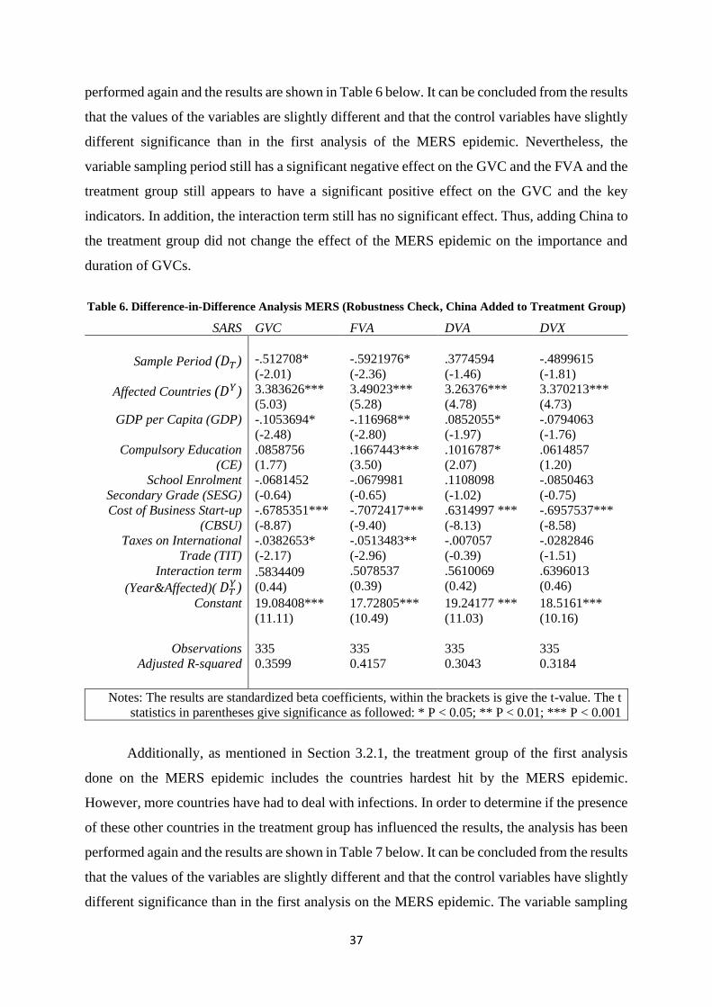
37

performed again and the results are shown in Table 6 below. It can be concluded from the results

that the values of the variables are slightly different and that the control variables have slightly

different significance than in the first analysis of the MERS epidemic. Nevertheless, the

variable sampling period still has a significant negative effect on the GVC and the FVA and the

treatment group still appears to have a significant positive effect on the GVC and the key

indicators. In addition, the interaction term still has no significant effect. Thus, adding China to

the treatment group did not change the effect of the MERS epidemic on the importance and

duration of GVCs.

Table 6. Difference-in-Difference Analysis MERS (Robustness Check, China Added to Treatment Group)

SARS GVC FVA DVA DVX

Sample Period (𝐷𝑇) -.512708*

(-2.01)

-.5921976*

(-2.36)

.3774594

(-1.46)

-.4899615

(-1.81)

Affected Countries (𝐷𝑌) 3.383626***

(5.03)

3.49023***

(5.28)

3.26376***

(4.78)

3.370213***

(4.73)

GDP per Capita (GDP) -.1053694*

(-2.48)

-.116968**

(-2.80)

.0852055*

(-1.97)

-.0794063

(-1.76)

Compulsory Education

(CE)

.0858756

(1.77)

.1667443***

(3.50)

.1016787*

(2.07)

.0614857

(1.20)

School Enrolment

Secondary Grade (SESG)

-.0681452

(-0.64)

-.0679981

(-0.65)

.1108098

(-1.02)

-.0850463

(-0.75)

Cost of Business Start-up

(CBSU)

-.6785351***

(-8.87)

-.7072417***

(-9.40)

.6314997 ***

(-8.13)

-.6957537***

(-8.58)

Taxes on International

Trade (TIT)

-.0382653*

(-2.17)

-.0513483**

(-2.96)

-.007057

(-0.39)

-.0282846

(-1.51)

Interaction term

(Year&Affected)( 𝐷𝑇𝑌)

.5834409

(0.44)

.5078537

(0.39)

.5610069

(0.42)

.6396013

(0.46)

Constant 19.08408***

(11.11)

17.72805***

(10.49)

19.24177 ***

(11.03)

18.5161***

(10.16)

Observations 335 335 335 335

Adjusted R-squared 0.3599 0.4157 0.3043 0.3184

Notes: The results are standardized beta coefficients, within the brackets is give the t-value. The t

statistics in parentheses give significance as followed: * P < 0.05; ** P < 0.01; *** P < 0.001

Additionally, as mentioned in Section 3.2.1, the treatment group of the first analysis

done on the MERS epidemic includes the countries hardest hit by the MERS epidemic.

However, more countries have had to deal with infections. In order to determine if the presence

of these other countries in the treatment group has influenced the results, the analysis has been

performed again and the results are shown in Table 7 below. It can be concluded from the results

that the values of the variables are slightly different and that the control variables have slightly

different significance than in the first analysis on the MERS epidemic. The variable sampling

38

period only has had a significant positive effect on the FVA, which differs from the findings in

the first analysis. Nevertheless, the results of the variable affected countries and the interaction

term are consistent with the findings in the first analysis, as the affected countries has a

significant positive result for the GVC and its main indicators, and the interaction term again

has no significant results. Thus, the MERS epidemic has still not had a significant long-term

effect on the importance of GVCs or the length of GVCs.

What’s more, part of the additional affected countries are European countries and the

USA. In order to determine if the presence of only these Western countries in the treatment

group has influenced the results, the analysis was performed again, and the results are also

shown in Table 7 below. The most important findings are that the results of the variable sample

period are not significant, which contradicts with the finding that the sample period has a

significant positive effect for the analysis done including all affected countries (the first results

in Table 7). Nonetheless, the affected countries once again have significant positive results for

the GVC, and its key indicators and the interaction term still has no significant results. Hence,

even in this situation, the MERS epidemic had no significant long-term effect on the importance

of GVCs or the length of GVCs.

In conclusion, the analyses of the impact of the MERS epidemic found that both the

importance of GVCs and the length of GVCs were not significantly affected by the epidemic.

Therefore, these findings are similar to the results concerning the SARS epidemic.

Consequently, these findings contradict the propositions made, as the crisis was expected to

have a negative impact on the importance and length of GVCs. Nonetheless, these findings are,

similar to the findings on the SARS epidemic, consistent with the expectation of Simola (2021)

and, Shingal and Argarwal (2020), that GVCs are well founded and unlikely to change as a

result of a crisis.

39

Table 7. Difference-in-Difference Analysis MERS (Robustness Check, All Affected Countries & Only

Western Affected Countries)

All Affected Countries SARS GVC FVA DVA DVX

Sample Period (𝐷𝑇) .4373072

(-1.83)

.5120459* (-2.23)

.3016688 (-1.21)

.4184607 (-1.63)

Affected Countries (𝐷𝑌) 3.147552***

(10.20)

3.29383*** (11.07)

2.950373*** (9.18)

3.130041*** (9.41)

GDP per Capita (GDP) .0708963

(-1.87)

.0806839* (-2.21)

-.053658 (-1.36)

.0449882 (-1.10)

Compulsory Education

(CE) .0869354*

(2.03)

.1684051*** (4.08)

.1018927* (2.29)

.0624337 (1.35)

School Enrolment

Secondary Grade (SESG) .1976656* (-2.10)

-.202111* (-2.23)

.2340357* (-2.39)

.2142218* (-2.11)

Cost of Business Start-up

(CBSU) -.692044***

(-10.24)

-.720737*** (-11.06)

.6451072*** (-9.17)

.7093175*** (-9.74)

Taxes on International

Trade (TIT) .0165452

(-1.06)

.0288186 (-1.92)

.0137061 (0.84)

.0066903 (-0.40)

Interaction term

(Year&Affected)( 𝐷𝑇𝑌)

.0273289

(0.04)

.0065624 (-0.01)

.0132454 (-0.02)

.069458 (0.10)

Constant 120.0063***

(13.29)

18.66242*** (12.87)

20.1521*** (12.86)

19.43869*** (11.99)

Observations 335 335 335 335

Adjusted R-squared 0.4969 0.5593 0.4260 0.4470

Western Affected Countries SARS GVC FVA DVA DVX

Sample Period (𝐷𝑇) .3980953 (-1.53)

.4838372 (-1.88)

.2675174 (-1.02)

.3724355 (-1.36)

Affected Countries (𝐷𝑌) 2.976403*** (4.48)

2.830165*** (4.30)

2.949359*** (4.39)

3.073289*** (4.38)

GDP per Capita (GDP) .1141826** (-2.63)

.1270417** (-2.96)

.0932459* (-2.13)

.0876846 (-1.92)

Compulsory Education

(CE) .0386956 (0.78)

.1200034* (2.45)

.0555758 (1.11)

.01356 (0.26)

School Enrolment

Secondary Grade (SESG) .1725792 (-1.59)

.1721919 (-1.60)

.2127702 (-1.93)

.1908601 (-1.66)

Cost of Business Start-up

(CBSU) .7098442*** (-9.10)

.7400457*** (-9.58)

.6611223*** (-8.38)

.7264991*** (-8.82)

Taxes on International

Trade (TIT) .0036496 (0.19)

.0106123 (-0.56)

.0342456 (1.78)

.014656 (0.73)

Interaction term

(Year&Affected)( 𝐷𝑇𝑌)

1.145484 (-0.73)

-1.20771 (-0.78)

-.973754 (-0.62)

-1.05255 (-0.64)

Constant

20.80841*** (12.00)

19.48876*** (11.35)

20.90818*** (11.92)

20.24334*** (11.06)

Observations 335 335 335 335

Adjusted R-squared 0.3315 0.3813 0.2793 0.2945

Notes: The results are standardized beta coefficients, within the brackets is give the t-value. The t

statistics in parentheses give significance as followed: * P < 0.05; ** P < 0.01; *** P < 0.001

40

4.3 Results Financial Crisis

This section will discuss the results of the panel regression analyses done on the effect of the

financial crisis on the importance of GVCs, shown in Table 8, and on the length of GVCs,

shown in Table 9 to 11. After discussing the results in Tables 8 to 11, the results of Table 12 to

15 will show the first robustness check for which the periods 2008-2009 and 2012-2016 are

taken as the crisis period. Then, the results in Table 16 to 19 show the results on having only

the period 2012-2016 as crisis period to see what the effect of the aftermath of the 2008 financial

crisis has been. To be complete, this study will include the results of both FE and RE, and the

Hausman test in the Appendix. As explained in chapter III, the results of the Hausman test

determine whether FE or RE should be used. Therefore, this section will show the results of the

test used, including the results of the Hausman test.

According to the results of the Hausman test in Table 8, it can be stated that the FE

model should be used as the p-value of the Hausman test is below 0.05. The FE model shows

that the financial crisis had a significantly positive effect on the amount of GVCs. The R-

squared results are given for the three types of variation and according to those, the correlation

is found to be not that strong. This could probably be because the model could be refined by

adding variables. Moreover, the variation between (R-squared (between)) appears to show the

most correlation, which means that across the countries there is an influence of the financial

crisis on GVCs. In addition, according to Rho, the variation in GVCs can be mostly related to

the differences between the countries. Furthermore, all three control variables appear to have

had a significantly negative effect on the amount of GVCs, which is in line with the literature

discussed in Chapter II. In other words, the results are in line with the theory behind drivers of

offshoring and reshoring. In conclusion, the financial crisis appears to have had a significant

positive effect on the importance of GVCs.

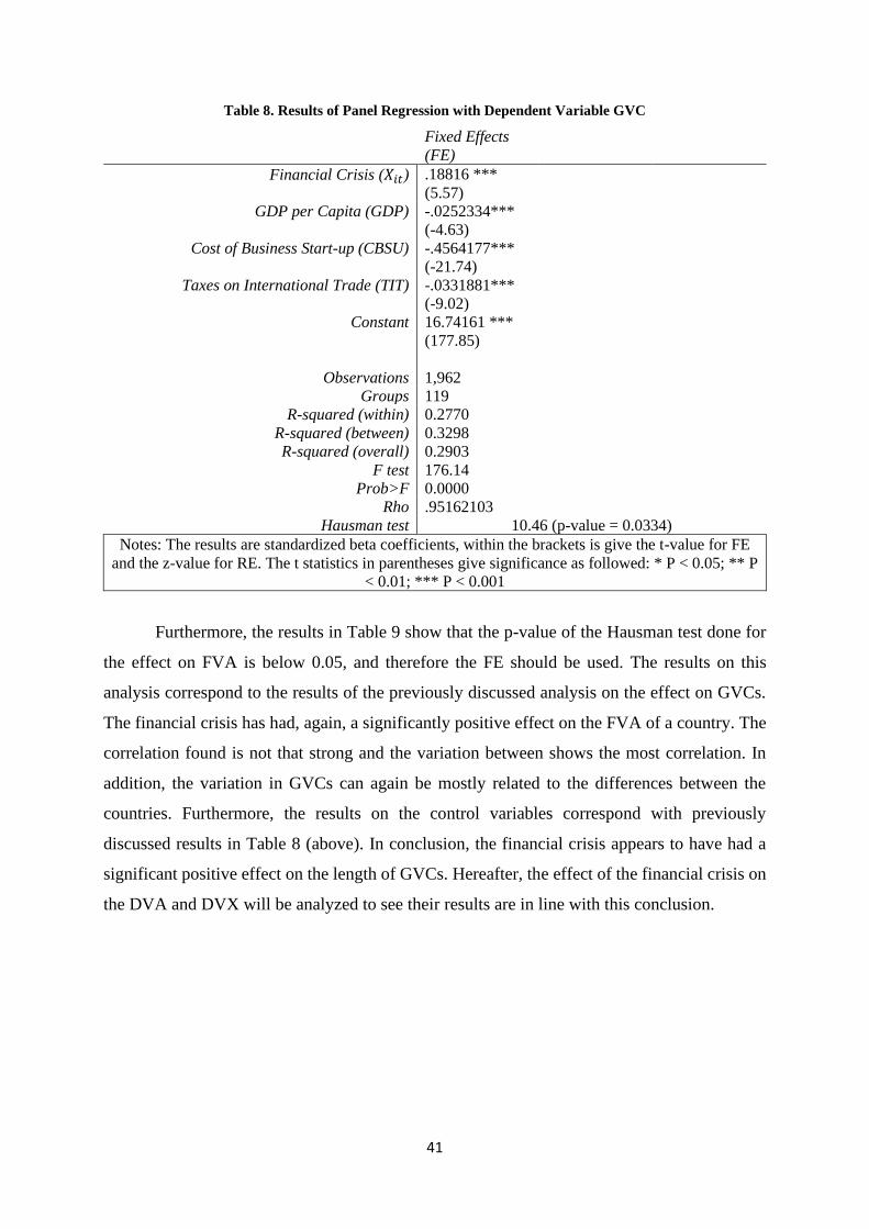
41

Table 8. Results of Panel Regression with Dependent Variable GVC

Fixed Effects

(FE)

Financial Crisis (𝑋𝑖𝑡) .18816 ***

(5.57)

GDP per Capita (GDP) -.0252334***

(-4.63)

Cost of Business Start-up (CBSU) -.4564177***

(-21.74)

Taxes on International Trade (TIT) -.0331881***

(-9.02)

Constant 16.74161 ***

(177.85)

Observations 1,962

Groups 119

R-squared (within) 0.2770

R-squared (between) 0.3298

R-squared (overall) 0.2903

F test 176.14

Prob>F 0.0000

Rho .95162103

Hausman test 10.46 (p-value = 0.0334)

Notes: The results are standardized beta coefficients, within the brackets is give the t-value for FE

and the z-value for RE. The t statistics in parentheses give significance as followed: * P < 0.05; ** P

< 0.01; *** P < 0.001

Furthermore, the results in Table 9 show that the p-value of the Hausman test done for

the effect on FVA is below 0.05, and therefore the FE should be used. The results on this

analysis correspond to the results of the previously discussed analysis on the effect on GVCs.

The financial crisis has had, again, a significantly positive effect on the FVA of a country. The

correlation found is not that strong and the variation between shows the most correlation. In

addition, the variation in GVCs can again be mostly related to the differences between the

countries. Furthermore, the results on the control variables correspond with previously

discussed results in Table 8 (above). In conclusion, the financial crisis appears to have had a

significant positive effect on the length of GVCs. Hereafter, the effect of the financial crisis on

the DVA and DVX will be analyzed to see their results are in line with this conclusion.

42

Table 9. Results of Panel Regression with Dependent Variable FVA

Fixed Effects

(FE)

Financial Crisis (𝑋𝑖𝑡) .1728261***

(4.97)

GDP per Capita (GDP) -.0227621***

(-4.05)

Cost of Business Start-up (CBSU) -.4610717***

(-21.31)

Taxes on International Trade (TIT) -.034333***

(-9.06)

Constant 15.78383***

(162.73)

Observations 1,962

Groups 119

R-squared (within) 0.2673

R-squared (between) 0.3828

R-squared (overall) 0.3336

F test 167.69

Prob>F 0.0000

Rho .95028085

Hausman test 20.87 (p-value = 0.0003)

Notes: The results are standardized beta coefficients, within the brackets is give the t-value for FE

and the z-value for RE. The t statistics in parentheses give significance as followed: * P < 0.05; ** P

< 0.01; *** P < 0.001

Moreover, since the results in Table 10 (below) show that the p-value of the Hausman

test done for the effect on DVA is above 0.05, it appears that the RE test should be used for this

analysis. The RE test shows that the financial crisis has had a significant positive effect on a

country’s DVA. Again, the R-squared results are given for the three types of variation and

according to those, the correlation is found to be not that strong. Moreover, the variation

between (R-squared (within)) appears again to show the most correlation, which means that

within the countries there is an influence of the financial crisis on DVA. In addition, as the RE

model is used Rho shows that the variation could be almost entirely explained by the constant

term. Furthermore, the results on the control variables correspond with the results in Table 9

(above). Again, all three control variables appear to have a significant negative effect on the

dependent variable, in this case DVA. Hence, these findings confirm the previously discussed

results of Table 9 (above) and the conclusion that the financial crisis has had a significant

positive effect on the length of GVCs.

43

Table 10. Results of Panel Regression with Dependent Variable DVA

Random Effects

(RE)

Financial Crisis (𝑋𝑖𝑡) .145595***

(4.65)

GDP per Capita (GDP) -.024193***

(-4.80)

Cost of Business Start-up (CBSU) -.4545849***

(-23.63)

Taxes on International Trade (TIT) -.0282004***

(-8.32)

Constant 17.20156***

(84.88)

Observations 1,962

Groups 119

R-squared (within) 0.2872

R-squared (between) 0.2658

R-squared (overall) 0.2419

Wald test 777.10

Prob>Chi2 0.0000

Rho .95612152

Hausman test 5.50 (p-value = 0.2393)

Notes: The results are standardized beta coefficients, within the brackets is give the t-value for FE

and the z-value for RE. The t statistics in parentheses give significance as followed: * P < 0.05; ** P

< 0.01; *** P < 0.001

Finally, the results in Table 11 (below) show that the p-value of the Hausman test done

for the effect on DVX is also above 0.05, and thus the RE test should be used. The results on

this RE test are, again, in line with the previously discussed results of Table 10 (above). The

financial crisis had a significant positive effect on the DVX of a country. The correlation found

is not that strong and the variation within shows the most correlation. In addition, Rho shows

here too that the variation could be almost entirely explained by the constant term. Thereby, the

control variables turn out to have, once again, a significant negative effect on the relevant key

indicator. These results lead to the conclusion that also this analysis supports the conclusion of

Table 9, the financial crisis has had a significant positive effect on the length of global value

chains.

44

Table 11. Results of Panel Regression with Dependent Variable DVX

Random Effects

(RE)

Financial Crisis (𝑋𝑖𝑡) .1997342***

(5.93)

GDP per Capita (GDP) -.0265028***

(-4.88)

Cost of Business Start-up (CBSU) -.4463552***

(-21.57)

Taxes on International Trade (TIT) -.0312003***

(-8.56)

Constant 16.16293***

(76.52)

Observations 1,962

Groups 119

R-squared (within) 0.2635

R-squared (between) 0.2883

R-squared (overall) 0.2577

Wald test 695.69

Prob>Chi2 0.0000

Rho .95268818

Hausman test 7.48 (p-value = 0.1124)

Notes: The results are standardized beta coefficients, within the brackets is give the t-value for FE

and the z-value for RE. The t statistics in parentheses give significance as followed: * P < 0.05; ** P

< 0.01; *** P < 0.001

As mentioned, the panel regressions are done again having the periods 2008-2009 and

2012-2016 as the crisis period to see if including the aftermath of the 2008 crisis influences the

analysis done. According to Table 12 (below), the Hausman test gives a p-value of 0.000 which

is below 0.05 and thus FE should be used. The FE model shows, again, that the crisis had a

significantly positive effect on the amount of GVCs. According to the R-squared results, the

correlation is found to be not that strong. Moreover, the variation within (R-squared (within))

appears to show the most correlation, which means that within the countries there is an influence

of the financial crisis on GVCs. In addition, according to Rho, the variation in GVCs can be

mostly related to the differences between the countries. Furthermore, all three control variables

appear to have had once more, a significantly negative effect on the amount of GVCs, which is

in line with the literature discussed in Chapter II. In other words, the results are again in line

with the theory behind drivers of offshoring and reshoring. This robustness check shows that

adding the aftermath to the crisis period yields results similar to those discussed above.

Therefore, one assumption is that the 2012-2016 period also had a significant positive effect on

the importance of GVCs. This will have to be shown in the next robustness check, shown in

Table 16.

45

Table 12. Results of Panel Regression with Dependent Variable GVC, Robustness check periods 2008-

2009 and 2012-2016 included as crisis period

Fixed Effects

(FE)

Financial Crisis (𝑋𝑖𝑡) .4614604***

(21.33)

GDP per Capita (GDP) -.0212451***

(-4.32)

Cost of Business Start-up (CBSU) -.4384211***

(-14.02)

Taxes on International Trade (TIT) -.02671***

(-8.02)

Constant 16.00885***

(173.98)

Observations 1,962

Groups 119

R-squared (within) 0.4106

R-squared (between) 0.3213

R-squared (overall) 0.2674

F test 320.32

Prob>F 0.0000

Rho .9636409

Hausman test 34.28 (p-value = 0.0000)

Notes: The results are standardized beta coefficients, within the brackets is give the t-value for FE

and the z-value for RE. The t statistics in parentheses give significance as followed: * P < 0.05; ** P

< 0.01; *** P < 0.001

Moreover, the results of the Hausman test in Table 13 show yet again that the FE should

be used. The results on this analysis correspond to the results of the previously discussed

analyses. The financial crisis has had, a significant positive effect on the FVA of a country. The

correlation found is not that strong and the variation between shows the most correlation. In

addition, the variation in GVCs can again be mostly related to the differences between the

countries. Furthermore, the results on the control variables correspond with previously

discussed results. In conclusion, adding the period 2012-2016 to the crisis period appears to

have had a significant positive effect on the length of GVCs. Hereafter, the effect of the

financial crisis on the DVA and DVX will indicate if this conclusion is correct.

46

Table 13. Results of Panel Regression with Dependent Variable FVA, Robustness check periods 2008-2009

and 2012-2016 included as crisis period

Fixed Effects

(FE)

Financial Crisis (𝑋𝑖𝑡) .4672491***

(20.92)

GDP per Capita (GDP) -.0187561***

(-3.69)

Cost of Business Start-up (CBSU) -.2898293***

(-13.71)

Taxes on International Trade (TIT) -.0276267***

(-8.03)

Constant 15.03958***

(158.28)

Observations 1,962

Groups 119

R-squared (within) 0.4002

R-squared (between) 0.3727

R-squared (overall) 0.3035

F test 306.70

Prob>F 0.0000

Rho .96306669

Hausman test 51.96 (p-value = 0.0000)

Notes: The results are standardized beta coefficients, within the brackets is give the t-value for FE

and the z-value for RE. The t statistics in parentheses give significance as followed: * P < 0.05; ** P

< 0.01; *** P < 0.001

Additionally, the results in Table 14 (below) show that the Hausman p-value is below

0.05, and therefore the FE test should be used for this analysis. The FE test shows that the

financial crisis has had a significant positive effect on a country’s DVA. The results on this

analysis correspond to the results of the previously discussed analysis on FVA. All in all, the

results confirm the conclusion above that adding the period 2012-2016 again shows a

significant positive effect of the crisis on the length of GVCs.

47

Table 14. Results of Panel Regression with Dependent Variable DVA, Robustness check periods 2008-

2009 and 2012-2016 included as crisis period

Fixed Effects

(FE)

Financial Crisis (𝑋𝑖𝑡) .4078319***

(20.21)

GDP per Capita (GDP) -.0204612***

(-4.46)

Cost of Business Start-up (CBSU) -.2990572***

(-15.66)

Taxes on International Trade (TIT) -.0220439***

(-7.09)

Constant 16.47502***

(191.93)

Observations 1,962

Groups 119

R-squared (within) 0.4100

R-squared (between) 0.2612

R-squared (overall) 0.2291

F test 319.45

Prob>F 0.0000

Rho .96618877

Hausman test 15.23 (p-value = 0.0042)

Notes: The results are standardized beta coefficients, within the brackets is give the t-value for FE

and the z-value for RE. The t statistics in parentheses give significance as followed: * P < 0.05; ** P

< 0.01; *** P < 0.001

The results in Table 15 (below) show that the Hausman p-value is yet again below 0.05,

and therefore the FE test should be used for this analysis. The FE test shows that also DVX has

been significant positively affected by the financial crisis. The results on this analysis

correspond to the results of the previously discussed analysis on FVA and DVA. These results

also confirm the conclusion that adding the period 2012-2016 shows a significant positive effect

of the crisis on the length of global value chains. Hereafter, the panel regression is done once

more on GVCs and the key indicators FVA, DVA and DVX but with only the period 2012-

2016 taken as the crisis period.

48

Table 15. Results of Panel Regression with Dependent Variable DVX, Robustness check periods 2008-

2009 and 2012-2016 included as crisis period

Fixed Effects

(FE)

Financial Crisis (𝑋𝑖𝑡) .4443725***

(20.41)

GDP per Capita (GDP) -.0223728***

(-4.52)

Cost of Business Start-up (CBSU) -.2747713***

(-13.34)

Taxes on International Trade (TIT) -.0245904***

(-7.33)

Constant 15.34936***

(165.77)

Observations 1,962

Groups 119

R-squared (within) 0.3880

R-squared (between) 0.2812

R-squared (overall) 0.2370

F test 291.52

Prob>F 0.0000

Rho .96453349

Hausman test 15.23 (p-value = 0.0042)

Notes: The results are standardized beta coefficients, within the brackets is give the t-value for FE

and the z-value for RE. The t statistics in parentheses give significance as followed: * P < 0.05; ** P

< 0.01; *** P < 0.001

To see if the period 2012-2016 has influenced the importance of GVCs, Table 16

(below) covers the results on the regression done for GVC. According to the Hausman p-value,

which is 0.0000, the FE model should be used. The regression gives results in line with the

previous regressions which means that also the period 2012-2016 has had a significant positive

effect on the importance of the GVCs. In other words, both the 2008 financial crisis and the

aftermath in 2012-2016 have brought about an increase in the total value of GVCs.

49

Table 16. Results of Panel Regression with Dependent Variable GVC, Robustness check period 2012-2016

as crisis period.

Fixed Effects

(FE)

Financial Crisis (𝑋𝑖𝑡) .4605601***

(18.53)

GDP per Capita (GDP) -.0204089***

(-4.04)

Cost of Business Start-up (CBSU) -.2770054***

(-12.82)

Taxes on International Trade (TIT) -.0305508***

(-8.98)

Constant 16.07018***

(169.53)

Observations 1,962

Groups 119

R-squared (within) 0.3805

R-squared (between) 0.3240

R-squared (overall) 0.2680

F test 282.37

Prob>F 0.0000

Rho .96173091

Hausman test 30.38 (p-value = 0.0000)

Notes: The results are standardized beta coefficients, within the brackets is give the t-value for FE

and the z-value for RE. The t statistics in parentheses give significance as followed: * P < 0.05; ** P

< 0.01; *** P < 0.001

Furthermore, to see if the period 2012-2016 has had an effect on the length of GVCs,

Table 17 (below) covers the results on the regression done for FVA. Once more, the Hausman

p-value has a value of 0.0000. Therefore, the FE model should be used again. The regression

gives results in line with the previous regressions which means that also the period 2012-2016

has had a significant positive effect on the length of the GVCs. Yet again, the same regression

done on DVA and DVX will show whether this is correct.

50

Table 17. Results of Panel Regression with Dependent Variable FVA, Robustness check period 2012-2016

as crisis period.

Fixed Effects

(FE)

Financial Crisis (𝑋𝑖𝑡) .4775147***

(18.71)

GDP per Capita (GDP) -.0178007***

(-3.43)

Cost of Business Start-up (CBSU) -.275549***

(-12.42)

Taxes on International Trade (TIT) -.0314138***

(-8.99)

Constant 15.08479***

(154.93)

Observations 1,962

Groups 119

R-squared (within) 0.3762

R-squared (between) 0.3767

R-squared (overall) 0.3039

F test 277.21

Prob>F 0.0000

Rho .96158922

Hausman test 45.72 (p-value = 0.0000)

Notes: The results are standardized beta coefficients, within the brackets is give the t-value for FE

and the z-value for RE. The t statistics in parentheses give significance as followed: * P < 0.05; ** P

< 0.01; *** P < 0.001

Additionally, the results in Table 18 (below) show that the Hausman p-value is below

0.05, and therefore the FE test should be used again. The FE test shows that the financial crisis

has had a significant positive effect on a country’s DVA. The results on this analysis correspond

to the results of the previously discussed analysis on FVA. In other words, the results confirm

the conclusion above that taking the period 2012-2016 as crisis period shows a significant

positive effect of the crisis on the length of GVCs.

51

Table 18. Results of Panel Regression with Dependent Variable DVA, Robustness check period 2012-2016

as crisis period.

Fixed Effects

(FE)

Financial Crisis (𝑋𝑖𝑡) .4202328***

(18.27)

GDP per Capita (GDP) -.0195939***

(-4.19)

Cost of Business Start-up (CBSU) -.2852838***

(-14.27)

Taxes on International Trade (TIT) -.025318***

(-8.04)

Constant 16.50928***

(188.21)

Observations 1,962

Groups 119

R-squared (within) 0.3897

R-squared (between) 0.2607

R-squared (overall) 0.2269

F test 293.62

Prob>F 0.0000

Rho .96511792

Hausman test 15.24 (p-value = 0.0042)

Notes: The results are standardized beta coefficients, within the brackets is give the t-value for FE

and the z-value for RE. The t statistics in parentheses give significance as followed: * P < 0.05; ** P

< 0.01; *** P < 0.001

Finally, the results in Table 19 (below) show that the Hausman p-value is yet again

below 0.05. The results of the FE test show that also DVX has been significant positively

affected by the period 2012-2016. The results on this analysis correspond to the results of the

previously discussed analysis on FVA and DVA. More specifically, the analyses confirm that

the period 2012-2016 has had a significant positive effect on the length of global value chains.

In conclusion, the analyses of the impact of the 2008 financial crisis found that both the

importance of GVCs and the length of GVCs were significantly affected by the financial crisis

and its aftermath. It is interesting to see that, when assuming that the pandemic will have a

similar effect on GVCs as the financial crisis of 2008, these findings are inconsistent with the

expectation of Simola (2021) and, Shingal and Argarwal (2020), that GVCs are well founded

and unlikely to change as a result of a crisis. Moreover, these findings completely contradict

the propositions made, as the crisis was expected to have a negative impact on the importance

and length of GVCs.

52

Table 19. Results of Panel Regression with Dependent Variable DVX, Robustness check period 2012-2016

as crisis period.

Fixed Effects

(FE)

Financial Crisis (𝑋𝑖𝑡) .4316201***

(17.22)

GDP per Capita (GDP) -.0216832***

(-4.26)

Cost of Business Start-up (CBSU) -.2697569***

(-12.38)

Taxes on International Trade (TIT) -.0283974***

(-8.27)

Constant 15.42637***

(161.32)

Observations 1,962

Groups 119

R-squared (within) 0.3536

R-squared (between) 0.2825

R-squared (overall) 0.2379

F test 251.45

Prob>F 0.0000

Rho .96244573

Hausman test 20.95 (p-value = 0.0003)

Notes: The results are standardized beta coefficients, within the brackets is give the t-value for FE

and the z-value for RE. The t statistics in parentheses give significance as followed: * P < 0.05; ** P

< 0.01; *** P < 0.001

53

V. Conclusion: Assessment of the Effect of COVID-19 on GVCs

This study has been set out with the aim of making a prediction on the effect of COVID-19 on

Global Values Chains. Based on analysis done with data of previously comparable crises, this

chapter will give an assessment of the potential effect of COVID-19 on GVCs. In addition, this

chapter will also discuss some limitations and, some opportunities for future research.

5.1 Assessment of the Effect of COVID-19 on GVCs

During this study it has become clear that understanding the effect of crises like the pandemic

is important for international trade, specifically for the existence of GVCs. When COVID-19

became a pandemic, countries took destructive measures against the spread of the virus which

affected GVCs as productions were put still and borders got closed. Hence, it is clear to say that

COVID-19 did influence GVCs during the pandemic. At the time of writing, the pandemic has

been going on for about a year and a half which means that the long-term effects are still unclear

as these cannot be substantiated from available data. Nevertheless, this study made two

propositions based on previous literature and with the help of data on previously comparable

crises quantitative research has been conducted.

The propositions made within this study suggest a negative effect of COVID-19 on the

importance and length of GVCs. Keeping these propositions in mind when looking at the results

in Chapter IV, it is interesting to see that for the difference-in-difference analyses on SARS the

results show no significant effects for the interaction term (years&affected). This suggests that

the SARS epidemic had no significant effect on the importance and the length of GVCs for

countries affected by the epidemic in the period after the crisis. Furthermore, robustness

analyses showed that having China in the treatment group had no significant effect on the

results. In other words, including a large country like China in the treatment group did not lead

to biased results for the effect of the SARS epidemic on the importance and length of GVCs.

Thus, if COVID-19 is expected to have the same effects on GVCs as SARS, this would be a

refutation of both propositions made.

Additionally, when looking at the results of the MERS epidemic it appears that this

epidemic did also have no significant effect on the importance and length of GVCs. Besides, as

China was a factor for the robustness analysis done for the effect of the SARS epidemic, a

similar robustness analysis was done for the MERS epidemic. More specifically, China was not

part of the affected countries by the MERS epidemic and therefore, the difference-in-difference

54

analysis was done again including China to see if including such a large country would have

had an effect on the results of the first analysis done on MERS. The results of this robustness

analysis concluded that adding China to the treatment group did not change the effect of the

MERS epidemic on the importance and duration of GVCs as found within the original analysis

done. Furthermore, the treatment group of the original analysis done on the effect of MERS

included only the included those countries that were hardest hit by the epidemic. However, the

spread of the virus has also reached many other countries, including some Western countries in

the E.U. and the U.S. (Middle East Respiratory Syndrome (MERS), 2019) Therefore, another

robustness check was conducted to measure whether the results differ when all affected

countries are included in the treatment group, compared to the first choice of treatment group.

This robustness analysis has shown that despite expanding the treatment group, MERS still

appears to have had no significant effect on the importance and length GVCs. Finally, the

analysis was conducted again using only the affected Western countries, including some

European countries and the U.S., to see if the impact of MERS would have been different if

only those countries had been affected. Also, in this case, however, it appears that MERS would

have had no significant long-term effect on the importance and length of GVCs. Thus, if

COVID-19 is expected to have the same effects on GVCs as MERS, this would also be a

refutation of both propositions made. Taking this into consideration and assuming that COVID-

19 will have the same effect on GVCs as the epidemics, neither of these propositions would

hold true. Thus, the pandemic is then expected to have no significant long-term effect on the

importance and length of GVCs.

By contrast, considering the results on the effect of the financial crisis in 2008 and 2009

on GVCs it appears that there were significant effects. More specifically, according to the

original regression analyses it appears that the period 2008 and 2009 has had a significant

positive effect on the importance and the length of GVCs which is a refutation of both

propositions as those suggested a negative effect. As the financial crisis has had a significant

aftermath in the post-crisis years, this study has done robustness checks to see if the aftermath

might have had an effect on the results of the analyses done. Therefore, a robustness analysis

was conducted with a different crisis period, inlcuding both the official period of the financial

crisis 2008-2009, and the aftermath period 2012-2016. This robustness analysis has shown

similar results as the original analysis done on the effect of the financial crisis. Thus, including

the aftermath period has also led to significant positive results. Thereafter, another analysis was

conducted in which the crisis period included only the aftermath period 2012-2016 to see what

the effect of the aftermath has been on the importance and length of GVCs. This later analyis

55

has also led to similar results. Hence, the aftermath has also had an significant positive effect

on the importance and length of GVCs. Taking this into consideration and assuming that

COVID-19 will have the same effect on GVCs as the financial crisis, neither of these

propositions would hold true. The pandemic is then expected to have a significant positive long-

term effect on the importance and length of GVCs.

Given these findings about the different crises and the resulting expectations, they are

contradictory. Nonetheless, as mentioned these previous crises did have some similarities with

the current pandemic but were not the entirely the same. Whereas the pandemic shows to have

similarities based on symptoms as the epidemics, the epidemics did not have the same

comprehensive effects as they did not hit worldwide. On the other hand, the financial crisis

might not have had the similar health effects, it did have a similar comprehensive effect. Since

this study is considering the effect of the pandemic on GVCs, which is a more economic effect,

the comparison made with the financial crisis is considered more valid also considering the

comprehensive effects of both types of crises. That is not to say, however, that the results of the

analyses on the epidemics are completely ignored. Therefore, based on the results of the

quantitative study, COVID-19 is expected to have a similar effect on the importance and length

of GVCs as the financial crisis, but to a lesser extent. In conclusion, this study expects COVID-

19 to have a small positive significant effect on GVCs in the long term.

5.2 Limitations

It should be acknowledged that this study is not free of limitations. The main limitation to this

research lies in the fact that there is no suitable data available because of the recency and

uniqueness of COVID-19. The data used belong to crises that are similar but not identical.

Consequently, it remains uncertain whether future data on COVID-19 will be comparable to

those for the crises used. Therefore, this study remains "only" a prediction based on some

similarities in characteristics between the epidemics/financial crisis and the pandemic.

What’s more, as previously discussed in Section 3.1, the GVC indicators are not a

perfect measure of the length of GVCs. The key indicators specify the value of the indicator,

which gives an indication of the length of GVCs, but not the exact number of border crossings

during a production process. Hence, the exact changes in length of GVCs cannot be measured

with the data used, only an indication is made.

56

5.3 Further Research

This thesis has laid a foundation for future research on the effect of COVID-19 on GVCs.

Within some time (months, years) more data on the effects of the pandemic will become

available which can be used to examine the real effect of COVID-19 on GVCs. In other words,

future research could be based on the limitations of this study, the suitability of data. As well,

it would be interesting to see what the effect of the pandemic would be having a better measure

of the length of GVCs. Additionally, future research could delve deeper into the impact of a

crisis like COVID-19 on the drivers of offshoring/reshoring, something this study did not get

to.

Besides, a suggestion for further research could be the effect of a crisis like the current

pandemic on the social importance of GVCs for emerging economies. The impact of GVCs

differs across developed and emerging economies. For developed economies, the participation

in GVCs gives access to economies of scale, as a result of producing on a large scale the

production costs will decrease. Thereby, inputs become more competitively priced and there is

more variety among products. For emerging economies, the participation in GVCs means, as

mentioned before, the ability to industrialize at a relatively fast rate. (Baldwin & Lopez-

Gonzalez, 2013) These statements are supported by theoretical literature in which studies have

shown that several channels can show productivity gains related to GVCs and offshoring.

(Caliendo & Parro, 2015; Grossman & Rossi-Hansberg, 2008; Halpern et al., 2015; Raei et al.,

2019) What’s more, previous empirical research has shown the macroeconomic impact of

GVCs on a country’s income. Moreover, it was found that participation in GVCs is positively

related to income per capita, productivity and investments. In addition, participation within

GVCs is strongly determined by institutional features. Though, it should be noticed that

participation in GVCs does not result in gains automatically. More specifically, heterogeneity

has been found between countries with different income levels. It appears that upper-middle

and high-income countries benefit more of GVC participation than lower-middle and low

income countries. (Raei et al., 2019) Therefore, it could be interesting for fueature research to

measure how much the progress of developing countries depends on the connections with other

countries through GVCs. And, to measure the effect of a crisis like COVID-19 on the progress

made by emerging economies as a result of involvement with GVCs.

57

References

Abadie, A. (2005). Semiparametric difference-in-differences estimators. The Review of Economic

Studies, 72(1), 1-19.

Baldwin, R. (2020, March 13). Keeping the lights on: Economic medicine for a medical shock.

Retrieved from voxeu: https://voxeu.org/article/how-should-we-think-about-containing-

covid-19-economic-crisis

Baldwin, R., & Lopez-Gonzalez, J. (2013). Supply‐chain trade: A portrait of global patterns and several

testable hypotheses. The World Economy, 38(11), 1682-1721.

Barbieri, P., Boffelli, A., Elia, S., Fratocchi, L., Kalchschmidt, M., & Samson, D. (2020). What can we

learn about reshoring after Covid-19? Operations Management Research, 131-136.

Benstead, A. V., Stevenson, M., & Hendry, L. C. (2017). Why and how do firms reshore? A

contingency-based conceptual framework. Operations Management Research, 82-103.

Bertrand, M., Duflo, E., & Mullainathan, S. (2004). How much should we trust differences-in-

differences estimates? The Quarterly journal of economics, 119(1), 249-75.

Caliendo, L., & Parro, F. (2015). Estimates of the Trade and Welfare Effects of NAFTA. The Review of

Economic Studies, 82(1), 1-44.

Carey, H. (2020, August 19). The Impact of Natural Disasters on Economy and Supply Chain — and

How to Prepare for the Worst. Retrieved from Thomas:

https://www.thomasnet.com/insights/how-natural-disasters-affect-the-supply-chain-and-

how-to-prepare-for-the-

worst/#:~:text=Whether%20facing%20a%20hurricane%2C%20tsunami,and%20unbalanced%

20supply%20and%20demand.

58

Casella, B., Bolwijn, R., Moran, D., & Kanemoto, K. (2019). Improving the analysis of global value

chains: the UNCTAD-Eora Database. Transnational Corporations, 26(3).

Castañeda-Navarette, J., Hauge, J., & López-Gómez, C. (2020). COVID-19's impacts on global value

chains, as seen in the apparel industry. Development Policy Review.

CEPII. (2021, February 19). BACI. Retrieved from CEPII Research and Expertise on the World

Economy: http://www.cepii.fr/cepii/en/bdd_modele/presentation.asp?id=37

Chief Economist Team. (2020). The impact of the Covid-19 pandemic on global and EU trade. .:

European Commission .

Danielsson, J., Macrae, R., Vayanos, D., & Zigrand, J. (2020, March 26). The coronavirus crisis is no

2008. Retrieved from voxeu: https://voxeu.org/article/coronavirus-crisis-no-2008

Dunning, J. H., & Lundan, S. M. (2008). Institutions and the OLI paradigm of the multinational

enterprise. Asia Pacific Journal of Management, 25(4), 573-93.

Feenstra, R., & Hanson, G. (1997). Productivity Measurement and the Impact of Trade and

Technology on Wages: Estimates for the U.S., 1972-1990. Cambridge: National Bureau of

Economic Research.

Frost, M. (2021). Middle East respiratory syndrome coronavirus (MERS-CoV). Retrieved from World

Health Organization: https://www.who.int/health-topics/middle-east-respiratory-syndrome-

coronavirus-mers#tab=tab_1

Grossman, G. M., & Rossi-Hansberg, E. (2008). Trading tasks: A simple theory of offshoring. American

Economic Review, 98(5), 1978-97.

Gurtu, A., Saxena, R., & Sah, N. (2019). Offshoring Decisions: A Comprehensive and Conceptual

Framework. Operations and Supply Chain Management: An International Journal, 12(3), 118-

28.

59

Halpern, L., Koren, M., & Szeidl, A. (2015). Imported inputs and productivity. American Economic

Review, 105(12), 3660-3703.

Hill, R. C., Griffiths, W. E., & Lim, G. C. (2008). Principles of Econometrics. John Wiley & Sons.

Juma'h, A. H., & Campus, M. (2007). Offshoring and Foreign Direct Investment. Revista Empresarial

Inter Metro/Inter Metro Business Journal, 50-61.

Koopman, R., Powers, W., Wang, Z., & Wei, S. J. (2010). Give credit where credit is due: Tracing value

added in global production chains. National Bureau of Economic Research.

Middle East Respiratory Syndrome (MERS). (2019, August 2). Centers for Disease Control and

Prevention. https://www.cdc.gov/coronavirus/mers/index.htmlMoriconi, S., Peri, G., &

Pozzoli, D. (2019, February 24). The role of regulations and immigration in firms' offshoring

decisions. Retrieved from VOXEU: https://voxeu.org/article/regulations-immigration-and-

firms-offshoring-decisions

Navaretti, G. B., & Venables, A. J. (2004). Multinational Firms in the World Economy. Princeton:

Princeton University Press.

OECD. (2013, June 10). Globalisation. Retrieved from Glossary of Statistical Terms:

https://stats.oecd.org/glossary/detail.asp?ID=1121

OECD. (2013). Interconnected Economies: Benefiting from Global Value Chains. OECD Publishing.

OECD. (2013, June 14). Offshoring. Retrieved from Glossary of Statistical Terms:

https://stats.oecd.org/glossary/detail.asp?ID=6271

OECD. (2021, February 1). Global Value Chains (GVCs). Retrieved from OECD:

https://www.oecd.org/sti/ind/global-value-chains.htm

60

Pietrasik, T. (2021). Severe Acute Respiratory Syndrome (SARS). Retrieved from World Health

Organization: https://www.who.int/health-topics/severe-acute-respiratory-

syndrome#tab=tab_2

Raei, M. F., Ignatenko, A., & Mircheva, M. (2019). Global value chains: What are the benefits and why

do countries participate? International Monetary Fund.

Seric, A., Görg, H., Wan-Hsin, L., & Windisch, M. (2021, January 07). Risk, resilience, and recalibration

in global value chains. Retrieved from VOXEU: https://voxeu.org/article/risk-resilience-and-

recalibration-global-value-chains

Shingal, A., & Agarwal, P. (2020, 12 08). Global value chain responses to previous health shocks:

Lessons for Covid-19. Retrieved from voxeu: https://voxeu.org/article/global-value-chain-

responses-previous-health-shocks

Simola, H. (2021, April). The Impact of Covid-19 on Global Value Chains. Retrieved from SUERF:

https://www.suerf.org/suer-policy-brief/22639/the-impact-of-covid-19-on-global-value-

chains

Strange, R. (2020). The 2020 Covid-19 pandemic and global value chains. Journal of Industrial and

Business Economics, 455-465.

Strange, R., & Magnani, G. (2018). Outsourcing, Offshoring And The Global Factory. The Routledge

companion to the geography of international business, 60-77.

The World Bank Group. (2021, 07 30). DataBank. Retrieved from The World Bank:

https://databank.worldbank.org/home.aspx

The World Bank Group. (2021, 07 30). Metadata Glossary. Retrieved from The World Bank:

https://databank.worldbank.org/metadataglossary/World-Development-Indicators/series

61

UNCTAD-Eora Global Value Chain Database. (2019). Retrieved from worldmrio:

https://worldmrio.com/unctadgvc/

University of Copenhagen;. (2019). Difference in Difference. Retrieved from Coursera:

https://www.coursera.org/lecture/causal-effects/lecture-5-difference-in-difference-RJZdk

Vandenbroucke-Grauls, C., Vandenbroucke, J., & Van der Meer, J. (2021). Epidemieën van

Besmettelijke Ziekten: Wat zegt de Wetenschap? Koninklijke Nederlandse Akademie van

Wetenschappen, Amsterdam.

World Bank, & World Trade Organization. (2019). Global Value Chain Development Report 2019 :

Technological Innovation, Supply Chain Trade, and Workers in a Globalized World (English).

Washington, D.C.: World Bank Group.

WTO. (2021, April 1). Global Value Chains. Retrieved from World Trade Organization:

https://www.wto.org/english/res_e/statis_e/miwi_e/miwi_e.htm

Wu, X., & Zhang, F. (2011, November 05). When Offshoring Backfires. Retrieved from VOXEU:

https://voxeu.org/article/when-offshoring-backfires

Zhan, J., Bolwijn, R., Casella, B., & Santos-Paulino, A. (2020). Global value chain transformation to

2030: Overall direction and policy implications. VoxEU & CEPR., .

62

Appendix A – Descriptive Statistics

Table A1. Descriptive Statistics - Unchanged

Variable Obs Mean Std. Dev. Min Max

Sample Period 5,510 2004 8.36736 1990 2018

GVC 5,510 3.41e+07 1.12e+08 0 1.47e+09

DVA 5,510 4.31e+07 1.47e+08 0 1.88e+09

FVA 5,510 1.71e+07 5.83e+07 0 8.75e+08

DVX 5,510 1.71e+07 5.84e+07 0 6.83e+08

GDP per Capita (GDP) 5,086 2674800 2821176 175.01 9988294

Compulsory Education (CE) 3,441 9.305434 2.184245 0 17

School Enrollment Secondary Grade

(SESG)

3,624 5005342 3478972 14.17 9999272

Cost of Business Start-up (CBSU) 2,519 49.58742 112.6142 0 1540.2

Taxes on International Trade (TIT) 2,859 2360290 2464059 -

158417

9962858

Table A2. Descriptive Statistics - Lognormal

Variable Obs Mean Std. Dev. Min Max

Sample Period 5,510 2004 8.36736 1990 2018

GVC 5,046 14.38704 2.73486 9.125872 21.10853

DVA 5,045 14.81998 2.713029 .6097656 21.35454

FVA 5,045 13.4497 2.814696 7.933797 20.58974

DVX 5,046 13.71213 2.817573

-

.2744368 20.342

GDP per Capita (GDP) 5,086 13.19492 2.578989 5.164843 16.11692

Compulsory Education (CE) 3,441 9.305434 2.184245 0 17

School Enrollment Secondary Grade

(SESG) 3,624 14.9647 1.265593 2.651127 16.11802

Cost of Business Start-up (CBSU) 2,498 2.658226 1.716273

-

2.302585 7.339667

Taxes on International Trade (TIT) 2,434 12.19475 6.23065

-

11.19084 16.11437

63

Table A3. Descriptive Statistics – Lognormal, Dummy variable adjustment used to correct for

missing data and still missing data dropped

Variable Obs Mean Std. Dev. Min Max

Sample Period 3,451 2004 8.367813 1990 2018

GVC 3,451 15.08144 2.653356 9.686575 21.10853

DVA 3,450 15.50734 2.503146 9.830916 21.35454

FVA 3,451 14.18775 2.753215 8.321178 20.58974

DVX 3,451 14.40543 2.647849 8.523175 20.342

GDP per Capita (GDP) 3,451 13.03087 2.61884 5.503297 16.11692

Compulsory Education (CE) 3,451 9.408355 2.090931 4 16

School Enrollment Secondary Grade

(SESG) 3,451 15.01927 1.175868 4.486837 16.11767

Cost of Business Start-up (CBSU) 3,430 2.327029 1.595675

-

2.436116 7.182656

Taxes on International Trade (TIT) 3,043 12.72586 5.6952

-

11.19084 16.11437

64

Appendix B –Regression Results on Panel Data

Table A4. Results of Panel Regression with Dependent Variable GVC

(Corresponds to Table 8)

Fixed Effects

(FE)

Random

Effects (RE)

Financial Crisis (𝑋𝑖𝑡) .18816 ***

(5.57)

.1877022***

(5.55)

GDP per Capita (GDP) -.0252334***

(-4.63)

-.0256221***

(-4.70)

Cost of Business Start-up (CBSU) -.4564177***

(-21.74)

-.4653999***

(-22.42)

Taxes on International Trade (TIT) -.0331881***

(-9.02)

-.0339278***

(-9.27)

Constant 16.74161 ***

(177.85)

16.8775***

(82.35)

Observations 1,962 1,962

Groups 119 119

R-squared (within) 0.2770 0.2770

R-squared (between) 0.3298 0.3298

R-squared (overall) 0.2903 0.2903

F test 176.14

Prob>F 0.0000

Wald test 749.35

Prob>Chi2 0.0000

Rho .95162103 .94874159

Hausman test 10.46 (p-value = 0.0334)

Notes: The results are standardized beta coefficients, within the brackets is give the t-value for FE

and the z-value for RE. The t statistics in parentheses give significance as followed: * P < 0.05; ** P

< 0.01; *** P < 0.001

65

Table A5. Results of Panel Regression with Dependent Variable FVA

(Corresponds to Table 9)

Fixed Effects

(FE)

Random

Effects (RE)

Financial Crisis (𝑋𝑖𝑡) .1728261***

(4.97)

.1721136***

(4.93)

GDP per Capita (GDP) -.0227621***

(-4.05)

-.0233764***

(-4.15)

Cost of Business Start-up (CBSU) -.4610717***

(-21.31)

-.4730217***

(-22.10)

Taxes on International Trade (TIT) -.034333***

(-9.06)

-.0354557***

(-9.39)

Constant 15.78383***

(162.73)

15.96486***

(78.20)

Observations 1,962 1,962

Groups 119 119

R-squared (within) 0.2673 0.2673

R-squared (between) 0.3828 0.3829

R-squared (overall) 0.3336 0.3337

F test 167.69

Prob>F 0.0000

Wald test 722.70

Prob>Chi2 0.0000

Rho .95028085 .94422127

Hausman test 20.87 (p-value = 0.0003)

Notes: The results are standardized beta coefficients, within the brackets is give the t-value for FE

and the z-value for RE. The t statistics in parentheses give significance as followed: * P < 0.05; ** P

< 0.01; *** P < 0.001

66

Table A6. Results of Panel Regression with Dependent Variable DVA

(Corresponds to Table 10)

Fixed Effects

(FE)

Random

Effects (RE)

Financial Crisis (𝑋𝑖𝑡) .145687***

(4.66)

.145595***

(4.65)

GDP per Capita (GDP) -.0239543***

(-4.75)

-.024193***

(-4.80)

Cost of Business Start-up (CBSU) -.4485563***

(-23.07)

-.4545849***

(-23.63)

Taxes on International Trade (TIT) -.0279382***

(-8.20)

-.0282004***

(-8.32)

Constant 17.1255***

(196.42)

17.20156***

(84.88)

Observations 1,962 1,962

Groups 119 119

R-squared (within) 0.2872 0.2872

R-squared (between) 0.2658 0.2658

R-squared (overall) 0.2419 0.2419

F test 185.23

Prob>F 0.0000

Wald test 777.10

Prob>Chi2 0.0000

Rho .956791 .95612152

Hausman test 5.50 (p-value = 0.2393)

Notes: The results are standardized beta coefficients, within the brackets is give the t-value for FE

and the z-value for RE. The t statistics in parentheses give significance as followed: * P < 0.05; ** P

< 0.01; *** P < 0.001

67

Table A7. Results of Panel Regression with Dependent Variable DVX

(Corresponds to Table 11)

Fixed Effects

(FE)

Random

Effects (RE)

Financial Crisis (𝑋𝑖𝑡) .2000084***

(5.94)

.1997342***

(5.93)

GDP per Capita (GDP) -.0262479***

(-4.83)

-.0265028***

(-4.88)

Cost of Business Start-up (CBSU) -.4384211***

(-20.95)

-.4463552***

(-21.57)

Taxes on International Trade (TIT) -.0306724***

(-8.37)

-.0312003***

(-8.56)

Constant 16.05254***

(171.10)

16.16293***

(76.52)

Observations 1,962 1,962

Groups 119 119

R-squared (within) 0.2635 0.2635

R-squared (between) 0.2883 0.2883

R-squared (overall) 0.2577 0.2577

F test 164.48

Prob>F 0.0000

Wald test 695.69

Prob>Chi2 0.0000

Rho .95427342 .95268818

Hausman test 7.48 (p-value = 0.1124)

Notes: The results are standardized beta coefficients, within the brackets is give the t-value for FE

and the z-value for RE. The t statistics in parentheses give significance as followed: * P < 0.05; ** P

< 0.01; *** P < 0.001

68

Table A8. Results of Panel Regression with Dependent Variable GVC, Robustness check periods 2008-

2009 and 2012-2016 included as crisis period

(Corresponds to Table 12)

Fixed Effects

(FE)

Random

Effects (RE)

Financial Crisis (𝑋𝑖𝑡) .4614604***

(21.33)

.4541187***

(20.95)

GDP per Capita (GDP) -.0212451***

(-4.32)

-.0217109***

(-4.39)

Cost of Business Start-up (CBSU) -.4384211***

(-14.02)

-.3008256***

(-14.82)

Taxes on International Trade (TIT) -.02671***

(-8.02)

-.0276533***

(-8.31)

Constant 16.00885***

(173.98)

16.19577***

(79.21)

Observations 1,962 1,962

Groups 119 119

R-squared (within) 0.4106 0.4105

R-squared (between) 0.3213 0.3220

R-squared (overall) 0.2674 0.2705

F test 320.32

Prob>F 0.0000

Wald test 1304.24

Prob>Chi2 0.0000

Rho .9636409 .95777832

Hausman test 34.28 (p-value = 0.0000)

Notes: The results are standardized beta coefficients, within the brackets is give the t-value for FE

and the z-value for RE. The t statistics in parentheses give significance as followed: * P < 0.05; ** P

< 0.01; *** P < 0.001

69

Table A9. Results of Panel Regression with Dependent Variable FVA, Robustness check periods 2008-

2009 and 2012-2016 included as crisis period

(Corresponds to Table 13)

Fixed Effects

(FE)

Random

Effects (RE)

Financial Crisis (𝑋𝑖𝑡) .4672491***

(20.92)

.4577587***

(20.40)

GDP per Capita (GDP) -.0187561***

(-3.69)

-.0194365***

(-3.80)

Cost of Business Start-up (CBSU) -.2898293***

(-13.71)

-.3074289***

(-14.64)

Taxes on International Trade (TIT) -.0276267***

(-8.03)

-.0289497***

(-8.41)

Constant 15.03958***

(158.28)

15.27466***

(74.97)

Observations 1,962 1,962

Groups 119 119

R-squared (within) 0.4002 0.3999

R-squared (between) 0.3727 0.3737

R-squared (overall) 0.3035 0.3081

F test 306.70

Prob>F 0.0000

Wald test 1250.15

Prob>Chi2 0.0000

Rho .96306669 .95376043

Hausman test 51.96 (p-value = 0.0000)

Notes: The results are standardized beta coefficients, within the brackets is give the t-value for FE

and the z-value for RE. The t statistics in parentheses give significance as followed: * P < 0.05; ** P

< 0.01; *** P < 0.001

70

Table A10. Results of Panel Regression with Dependent Variable DVA, Robustness check periods 2008-

2009 and 2012-2016 included as crisis period

(Corresponds to Table 14)

Fixed Effects

(FE)

Random

Effects (RE)

Financial Crisis (𝑋𝑖𝑡) .4078319***

(20.21)

.4029825***

(19.97)

GDP per Capita (GDP) -.0204612***

(-4.46)

-.0207656***

(-4.51)

Cost of Business Start-up (CBSU) -.2990572***

(-15.66)

-.3087932***

(-16.31)

Taxes on International Trade (TIT) -.0220439***

(-7.09)

-.0225098***

(-7.26)

Constant 16.47502***

(191.93)

16.59443***

(81.97)

Observations 1,962 1,962

Groups 119 119

R-squared (within) 0.4100 0.4099

R-squared (between) 0.2612 0.2614

R-squared (overall) 0.2291 0.2305

F test 319.45

Prob>F 0.0000

Wald test 1300.53

Prob>Chi2 0.0000

Rho .96618877 .96345229

Hausman test 15.23 (p-value = 0.0042)

Notes: The results are standardized beta coefficients, within the brackets is give the t-value for FE

and the z-value for RE. The t statistics in parentheses give significance as followed: * P < 0.05; ** P

< 0.01; *** P < 0.001

71

Table A11. Results of Panel Regression with Dependent Variable DVX, Robustness check periods 2008-

2009 and 2012-2016 included as crisis period

(Corresponds to Table 15)

Fixed Effects

(FE)

Random

Effects (RE)

Financial Crisis (𝑋𝑖𝑡) .4443725***

(20.41)

.4379915***

(20.10)

GDP per Capita (GDP) -.0223728***

(-4.52)

-.0227166***

(-4.57)

Cost of Business Start-up (CBSU) -.2747713***

(-13.34)

-.2872289***

(-14.07)

Taxes on International Trade (TIT) -.0245904***

(-7.33)

-.0253306***

(-7.57)

Constant 15.34936***

(165.77)

15.50822***

(73.48)

Observations 1,962 1,962

Groups 119 119

R-squared (within) 0.3880 0.3879

R-squared (between) 0.2812 0.2817

R-squared (overall) 0.2370 0.2395

F test 291.52

Prob>F 0.0000

Wald test 1187.08

Prob>Chi2 0.0000

Rho .96453349 .96034466

Hausman test 15.23 (p-value = 0.0042)

Notes: The results are standardized beta coefficients, within the brackets is give the t-value for FE

and the z-value for RE. The t statistics in parentheses give significance as followed: * P < 0.05; ** P

< 0.01; *** P < 0.001

72

Table A12. Results of Panel Regression with Dependent Variable GVC, Robustness check period 2012-

2016 as crisis period.

(Corresponds to Table 16)

Fixed Effects

(FE)

Random

Effects (RE)

Financial Crisis (𝑋𝑖𝑡) .4605601***

(18.53)

.4512414***

(18.13)

GDP per Capita (GDP) -.0204089***

(-4.04)

-.020923***

(-4.13)

Cost of Business Start-up (CBSU) -.2770054***

(-12.82)

-.2924273***

(-13.67)

Taxes on International Trade (TIT) -.0305508***

(-8.98)

-.0314397***

(-9.26)

Constant 16.07018***

(169.53)

16.25497***

(79.00)

Observations 1,962 1,962

Groups 119 119

R-squared (within) 0.3805 0.3803

R-squared (between) 0.3240 0.3246

R-squared (overall) 0.2680 0.2712

F test 282.37

Prob>F 0.0000

Wald test 1154.74

Prob>Chi2 0.0000

Rho .96173091 .95579462

Hausman test 30.38 (p-value = 0.0000)

Notes: The results are standardized beta coefficients, within the brackets is give the t-value for FE

and the z-value for RE. The t statistics in parentheses give significance as followed: * P < 0.05; ** P

< 0.01; *** P < 0.001

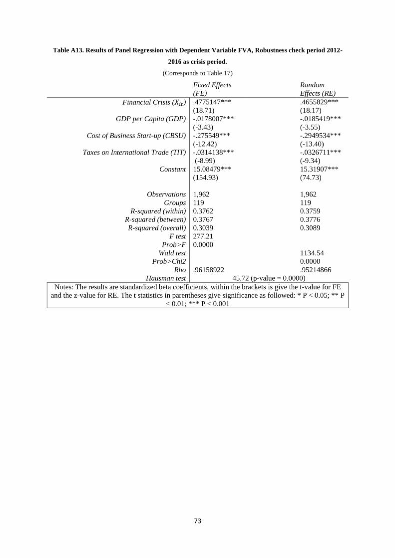
73

Table A13. Results of Panel Regression with Dependent Variable FVA, Robustness check period 2012-

2016 as crisis period.

(Corresponds to Table 17)

Fixed Effects

(FE)

Random

Effects (RE)

Financial Crisis (𝑋𝑖𝑡) .4775147***

(18.71)

.4655829***

(18.17)

GDP per Capita (GDP) -.0178007***

(-3.43)

-.0185419***

(-3.55)

Cost of Business Start-up (CBSU) -.275549***

(-12.42)

-.2949534***

(-13.40)

Taxes on International Trade (TIT) -.0314138***

(-8.99)

-.0326711***

(-9.34)

Constant 15.08479***

(154.93)

15.31907***

(74.73)

Observations 1,962 1,962

Groups 119 119

R-squared (within) 0.3762 0.3759

R-squared (between) 0.3767 0.3776

R-squared (overall) 0.3039 0.3089

F test 277.21

Prob>F 0.0000

Wald test 1134.54

Prob>Chi2 0.0000

Rho .96158922 .95214866

Hausman test 45.72 (p-value = 0.0000)

Notes: The results are standardized beta coefficients, within the brackets is give the t-value for FE

and the z-value for RE. The t statistics in parentheses give significance as followed: * P < 0.05; ** P

< 0.01; *** P < 0.001

74

Table A14. Results of Panel Regression with Dependent Variable DVA, Robustness check period 2012-

2016 as crisis period.

(Corresponds to Table 18)

Fixed Effects

(FE)

Random

Effects (RE)

Financial Crisis (𝑋𝑖𝑡) .4202328***

(18.27)

.413987***

(18.01)

GDP per Capita (GDP) -.0195939***

(-4.19)

-.0199288***

(-4.26)

Cost of Business Start-up (CBSU) -.2852838***

(-14.27)

-.2960643***

(-14.96)

Taxes on International Trade (TIT) -.025318***

(-8.04)

-.0257356***

(-8.20)

Constant 16.50928***

(188.21)

16.62686***

(81.81)

Observations 1,962 1,962

Groups 119 119

R-squared (within) 0.3897 0.3897

R-squared (between) 0.2607 0.2611

R-squared (overall) 0.2269 0.2285

F test 293.62

Prob>F 0.0000

Wald test 1197.47

Prob>Chi2 0.0000

Rho .96511792 .96227152

Hausman test 15.24 (p-value = 0.0042)

Notes: The results are standardized beta coefficients, within the brackets is give the t-value for FE

and the z-value for RE. The t statistics in parentheses give significance as followed: * P < 0.05; ** P

< 0.01; *** P < 0.001

75

Table A15. Results of Panel Regression with Dependent Variable DVX, Robustness check period 2012-

2016 as crisis period.

(Corresponds to Table 19)

Fixed Effects

(FE)

Random

Effects (RE)

Financial Crisis (𝑋𝑖𝑡) .4316201***

(17.22)

.423483***

(16.89)

GDP per Capita (GDP) -.0216832***

(-4.26)

-.0220659***

(-4.32)

Cost of Business Start-up (CBSU) -.2697569***

(-12.38)

-.2835207***

(-13.14)

Taxes on International Trade (TIT) -.0283974***

(-8.27)

-.029084***

(-8.50)

Constant 15.42637***

(161.32)

15.58199***

(73.39)

Observations 1,962 1,962

Groups 119 119

R-squared (within) 0.3536 0.3534

R-squared (between) 0.2825 0.2831

R-squared (overall) 0.2379 0.2404

F test 251.45

Prob>F 0.0000

Wald test 1028.90

Prob>Chi2 0.0000

Rho .96244573 .95823012

Hausman test 20.95 (p-value = 0.0003)

Notes: The results are standardized beta coefficients, within the brackets is give the t-value for FE

and the z-value for RE. The t statistics in parentheses give significance as followed: * P < 0.05; ** P

< 0.01; *** P < 0.001