The Effect Of Dynamic Pricing And Revenue Management On

University of Pennsylvania University of Pennsylvania

ScholarlyCommons ScholarlyCommons

Publicly Accessible Penn Dissertations

2018

The Effect Of Dynamic Pricing And Revenue Management On The Effect Of Dynamic Pricing And Revenue Management On

Agent Behavior And Customer Perception Agent Behavior And Customer Perception

Xingwei Lu University of Pennsylvania, [email protected]

Follow this and additional works at: https://repository.upenn.edu/edissertations

Part of the Operational Research Commons

Recommended Citation Recommended Citation Lu, Xingwei, "The Effect Of Dynamic Pricing And Revenue Management On Agent Behavior And Customer Perception" (2018). Publicly Accessible Penn Dissertations. 2847. https://repository.upenn.edu/edissertations/2847

This paper is posted at ScholarlyCommons. https://repository.upenn.edu/edissertations/2847 For more information, please contact [email protected].

https://repository.upenn.edu/

https://repository.upenn.edu/edissertations

https://repository.upenn.edu/edissertations?utm_source=repository.upenn.edu%2Fedissertations%2F2847&utm_medium=PDF&utm_campaign=PDFCoverPages

http://network.bepress.com/hgg/discipline/308?utm_source=repository.upenn.edu%2Fedissertations%2F2847&utm_medium=PDF&utm_campaign=PDFCoverPages

https://repository.upenn.edu/edissertations/2847?utm_source=repository.upenn.edu%2Fedissertations%2F2847&utm_medium=PDF&utm_campaign=PDFCoverPages

https://repository.upenn.edu/edissertations/2847

mailto:[email protected]

The Effect Of Dynamic Pricing And Revenue Management On Agent Behavior And The Effect Of Dynamic Pricing And Revenue Management On Agent Behavior And Customer Perception Customer Perception

Abstract Abstract My dissertation extends the traditional fields of revenue management and dynamic pricing to newer markets. Specifically, my first two chapters explore the revenue management strategies and their impacts in the airline industry in the presence of loyalty programs. The first chapter solves the optimal revenue management algorithms when the firm is rewarding frequent customers with free capacity. Using a game-theoretic Littlewood model, we show that limiting award capacity can increase profits by enhancing loyalty award values; airlines can benefit from transitioning from mileage-based programs to revenue-based programs by simplifying its revenue management algorithm and allowing 100% award availability. The second chapter investigates customers' evaluations of loyalty program points. By fitting a Multinomial Logit model on DB1B data set, we calibrate customers' valuations for loyalty points at the issuance and redemption. We have two main conclusions: consumers are rational about the value of miles at issuance, but underestimate and overspend miles at redemption; higher award availability and more award choices lead to higher values of Loyalty points. Finally, my third chapter examines the impact of dynamic pricing in the ride-sharing economy. By using actual Uber pricing and partner data, the paper shows that ride-sharing platforms can efficiently signal market conditions, stimulate desirable agents' behavior, and reduce marketplace frictions through dynamic pricing.

Degree Type Degree Type Dissertation

Degree Name Degree Name Doctor of Philosophy (PhD)

Graduate Group Graduate Group Operations & Information Management

First Advisor First Advisor Xuanming Su

Keywords Keywords DYNAMIC PRICING, REVENUE MANAGEMENT, STRATEGIC CONSUMERS

Subject Categories Subject Categories Operational Research

This dissertation is available at ScholarlyCommons: https://repository.upenn.edu/edissertations/2847

https://repository.upenn.edu/edissertations/2847

THE EFFECT OF DYNAMIC PRICING AND REVENUE MANAGEMENT ON

AGENT BEHAVIOR AND CUSTOMER PERCEPTION

Xingwei Lu

A DISSERTATION

in

Operations, Information and Decisions

For the Graduate Group in Managerial Science and Applied Economics

Presented to the Faculties of the University of Pennsylvania

in

Partial Fulfillment of the Requirements for the

Degree of Doctor of Philosophy

2018

Supervisor of Dissertation

Xuanming Su, Murrel J. Ades Professor; Professor of Operations, Information and Decisions

Graduate Group Chairperson

Catherine Schrand, Celia Z. Moh Professor, Professor of Accounting

Dissertation Committee

Gerard P. Cachon, Fred R. Sullivan Professor of Operations, Information and Decisions; Professor ofMarketingMarshall L. Fisher, UPS Professor; Professor of Operations, Information and DecisionsMorris A. Cohen, Panasonic Professor of Manufacturing & Logistics; Co-Director, Fishman-DavidsonCenter for Service and Operations Management; Professor of Operations, Information and Decisions



c© COPYRIGHT

2018

Xingwei Lu

Dedicated to My Parents

iii

ABSTRACT



Xingwei Lu

Xuanming Su

My dissertation extends the traditional fields of revenue management and dynamic pricing

to newer markets. Specifically, my first two chapters explore the revenue management

strategies and their impacts in the airline industry in the presence of loyalty programs. The

first chapter solves the optimal revenue management algorithms when the firm is rewarding

frequent customers with free capacity. Using a game-theoretic Littlewood model, we show

that limiting award capacity can increase profits by enhancing loyalty award values; airlines

can benefit from transitioning from mileage-based programs to revenue-based programs by

simplifying its revenue management algorithm and allowing 100% award availability. The

second chapter investigates customers’ evaluations of loyalty program points. By fitting a

Multinomial Logit model on DB1B data set, we calibrate customers’ valuations for loyalty

points at the issuance and redemption. We have two main conclusions: consumers are

rational about the value of miles at issuance, but underestimate and overspend miles at

redemption; higher award availability and more award choices lead to higher values of

Loyalty points. Finally, my third chapter examines the impact of dynamic pricing in the

ride-sharing economy. By using actual Uber pricing and partner data, the paper shows that

ride-sharing platforms can efficiently signal market conditions, stimulate desirable agents’

behavior, and reduce marketplace frictions through dynamic pricing.

iv

Contents

ABSTRACT . . . . . . . . . . . . . . . . . . . . . . . . . . . . . . . . . . . . . . . . iv

LIST OF TABLES . . . . . . . . . . . . . . . . . . . . . . . . . . . . . . . . . . . . . vii

LIST OF ILLUSTRATIONS . . . . . . . . . . . . . . . . . . . . . . . . . . . . . . . ix

CHAPTER 1 : REVENUE MANAGEMENT WITH LOYALTY PROGRAMS . . 1

1.1 Introduction . . . . . . . . . . . . . . . . . . . . . . . . . . . . . . . . . . . . 1

1.2 Literature Review . . . . . . . . . . . . . . . . . . . . . . . . . . . . . . . . 5

1.3 Behavioral Evidence of Consumer Model . . . . . . . . . . . . . . . . . . . . 9

1.4 Firm’s Model and Equilibrium . . . . . . . . . . . . . . . . . . . . . . . . . 16

1.5 Volume-Based Loyalty Programs . . . . . . . . . . . . . . . . . . . . . . . . 19

1.6 Expense-Based Loyalty Programs . . . . . . . . . . . . . . . . . . . . . . . . 23

1.7 Point-Based Loyalty Programs . . . . . . . . . . . . . . . . . . . . . . . . . 25

1.8 Numerical Examples . . . . . . . . . . . . . . . . . . . . . . . . . . . . . . . 27

1.9 Conclusions . . . . . . . . . . . . . . . . . . . . . . . . . . . . . . . . . . . . 33

1.10 Appendix: Proofs . . . . . . . . . . . . . . . . . . . . . . . . . . . . . . . . . 40

CHAPTER 2 : LOYALTY PROGRAMS AND CONSUMER CHOICE: EVIDENCE

FROM AIRLINE INDUSTRY . . . . . . . . . . . . . . . . . . . . . 50

2.1 Introduction . . . . . . . . . . . . . . . . . . . . . . . . . . . . . . . . . . . . 50

2.2 Data . . . . . . . . . . . . . . . . . . . . . . . . . . . . . . . . . . . . . . . . 53

2.3 Methods . . . . . . . . . . . . . . . . . . . . . . . . . . . . . . . . . . . . . . 56

2.4 Results: Value of Miles . . . . . . . . . . . . . . . . . . . . . . . . . . . . . . 62

2.5 Counterfactual Analysis . . . . . . . . . . . . . . . . . . . . . . . . . . . . . 70

2.6 Conclusions . . . . . . . . . . . . . . . . . . . . . . . . . . . . . . . . . . . . 73

v

CHAPTER 3 : THE EFFECT OF DYNAMIC PRICING ON UBER’S DRIVER-

PARTNERS . . . . . . . . . . . . . . . . . . . . . . . . . . . . . . . 77

3.1 Introduction . . . . . . . . . . . . . . . . . . . . . . . . . . . . . . . . . . . . 77

3.2 Methodology . . . . . . . . . . . . . . . . . . . . . . . . . . . . . . . . . . . 80

3.3 Results . . . . . . . . . . . . . . . . . . . . . . . . . . . . . . . . . . . . . . . 93

3.4 Conclusions . . . . . . . . . . . . . . . . . . . . . . . . . . . . . . . . . . . . 97

vi

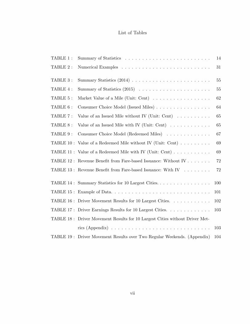
List of Tables

TABLE 1 : Summary of Statistics . . . . . . . . . . . . . . . . . . . . . . . . . 14

TABLE 2 : Numerical Examples . . . . . . . . . . . . . . . . . . . . . . . . . . 31

TABLE 3 : Summary Statistics (2014) . . . . . . . . . . . . . . . . . . . . . . . 55

TABLE 4 : Summary of Statistics (2015) . . . . . . . . . . . . . . . . . . . . . 55

TABLE 5 : Market Value of a Mile (Unit: Cent) . . . . . . . . . . . . . . . . . 62

TABLE 6 : Consumer Choice Model (Issued Miles) . . . . . . . . . . . . . . . . 64

TABLE 7 : Value of an Issued Mile without IV (Unit: Cent) . . . . . . . . . . 65

TABLE 8 : Value of an Issued Mile with IV (Unit: Cent) . . . . . . . . . . . . 65

TABLE 9 : Consumer Choice Model (Redeemed Miles) . . . . . . . . . . . . . 67

TABLE 10 : Value of a Redeemed Mile without IV (Unit: Cent) . . . . . . . . . 69

TABLE 11 : Value of a Redeemed Mile with IV (Unit: Cent) . . . . . . . . . . . 69

TABLE 12 : Revenue Benefit from Fare-based Issuance: Without IV . . . . . . . 72

TABLE 13 : Revenue Benefit from Fare-based Issuance: With IV . . . . . . . . 72

TABLE 14 : Summary Statistics for 10 Largest Cities. . . . . . . . . . . . . . . . 100

TABLE 15 : Example of Data. . . . . . . . . . . . . . . . . . . . . . . . . . . . . 101

TABLE 16 : Driver Movement Results for 10 Largest Cities. . . . . . . . . . . . 102

TABLE 17 : Driver Earnings Results for 10 Largest Cities. . . . . . . . . . . . . 103

TABLE 18 : Driver Movement Results for 10 Largest Cities without Driver Met-

rics (Appendix) . . . . . . . . . . . . . . . . . . . . . . . . . . . . . 103

TABLE 19 : Driver Movement Results over Two Regular Weekends. (Appendix) 104

vii

List of Figures

FIGURE 1 : Willingness to Pay . . . . . . . . . . . . . . . . . . . . . . . . . . . 14

FIGURE 2 : Equilibrium Timeline . . . . . . . . . . . . . . . . . . . . . . . . . 20

FIGURE 3 : Price Distribution . . . . . . . . . . . . . . . . . . . . . . . . . . . 28

FIGURE 4 : Profit Benefit of Loyalty Programs (Unit: %) . . . . . . . . . . . . 32

FIGURE 5 : Value of Issued Miles . . . . . . . . . . . . . . . . . . . . . . . . . 65

FIGURE 6 : Value of Redeemed Miles . . . . . . . . . . . . . . . . . . . . . . . 68

FIGURE 7 : Screenshot of the surge heatmap in the Uber driver app. The surge

heatmap shows the current value of the surge multiplier in each

hexagon to driver partners. . . . . . . . . . . . . . . . . . . . . . . 83

FIGURE 8 : The figure illustrates a driver at an origin hexagon i (outlined in

blue) choosing which hexagon to move to next (adjacent hexagons

are outlined in green). We model this choice as being correlated

with the change in smoothed surge multiplier (shown at right) be-

tween the origin hexagon and the 3 hexagons in the chosen direction

of motion. . . . . . . . . . . . . . . . . . . . . . . . . . . . . . . . 84

FIGURE 9 : Surge Multipliers Over Time: The left-hand plot shows the per-

centage of drivers’ earnings that were due to surge on the outage

weekend and the previous non-outage weekend in each of the cities

in our analysis. The right-hand plot similarly shows the percentage

of surged trips between the two weekends and across cities. . . . . 92

FIGURE 10 : Differences by Operating System: The figures show the tenure (left)

and age (right) for iOS and Android Drivers, by city. Confidence

intervals for the mean value are shown using the standard deviation

of the sample mean. . . . . . . . . . . . . . . . . . . . . . . . . . 93

viii

FIGURE 11 : Impact of Surge Information on Movement (%) . . . . . . . . . . 95

FIGURE 12 : Effects of Self-Positioning on Total Earnings (%) . . . . . . . . . . 96

FIGURE 13 : Effects of Self-Positioning on Surged Earnings (%) . . . . . . . . . 96

ix

CHAPTER 1 : REVENUE MANAGEMENT WITH LOYALTY PROGRAMS

This paper studies loyalty programs in firms such as airlines and hotels, where limited ca-

pacity is commonplace and revenue management is crucial. Based on Littlewood’s classic

two-type model, our model additionally reserves some capacity for rewards and allows cus-

tomers to choose between paying with cash and redeeming with points. We have three

conclusions. First, we show that revenue management algorithms need to be adjusted to

include award liability, i.e. the cost of issuing points to customers. However, the adjustment

can be neglected if the number of issued points is proportional the customers’ purchasing

price. Second, the optimal award capacity is constrained by a fixed level of redemption

probability in loyalty points. However, the redemption probability can be as high as 100%

if the number of redeemed points is proportional to the price. Finally, several airlines

(American, United and Delta) recently switched from rewarding customers based on their

purchasing quantity (volume-based) to rewarding them based on their purchasing expense

(expense-based). Other airlines (Southwest and JetBlue) decide both the issuance and re-

demption based on the purchasing price (point-based programs). We compare the pros

and cons of these program schemes. We show that volume-based schemes enhance profits

but generate accounting challenges. Expense-based schemes maintain profitability while

eliminating accounting challenges. Point-based schemes lose these profits in return for high

customer satisfaction, with a 100% award availability.

1.1. Introduction

Loyalty programs are ubiquitous among service firms such as airlines, hotels and rental

businesses. Well-known examples include American Airlines AAdvantage, Hilton HHonors,

and Hertz Gold Plus, all of which reward frequent patronage with free services. Whether

they are free flights or free hotel stays, loyalty rewards all take up capacity, which is a

constrained resource in service firms. While firms strive to fulfill their obligation of giving

out rewards to eligible customers, they have to accept the reality that every reward may

1

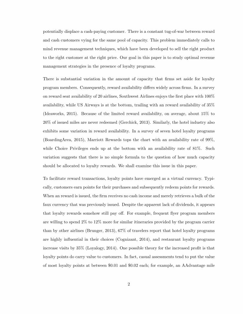
potentially displace a cash-paying customer. There is a constant tug-of-war between reward

and cash customers vying for the same pool of capacity. This problem immediately calls to

mind revenue management techniques, which have been developed to sell the right product

to the right customer at the right price. Our goal in this paper is to study optimal revenue

management strategies in the presence of loyalty programs.

There is substantial variation in the amount of capacity that firms set aside for loyalty

program members. Consequently, reward availability differs widely across firms. In a survey

on reward seat availability of 20 airlines, Southwest Airlines enjoys the first place with 100%

availability, while US Airways is at the bottom, trailing with an reward availability of 35%

(Ideaworks, 2015). Because of the limited reward availability, on average, about 15% to

20% of issued miles are never redeemed (Gerchick, 2013). Similarly, the hotel industry also

exhibits some variation in reward availability. In a survey of seven hotel loyalty programs

(BoardingArea, 2015), Marriott Rewards tops the chart with an availability rate of 99%,

while Choice Privileges ends up at the bottom with an availability rate of 81%. Such

variation suggests that there is no simple formula to the question of how much capacity

should be allocated to loyalty rewards. We shall examine this issue in this paper.

To facilitate reward transactions, loyalty points have emerged as a virtual currency. Typi-

cally, customers earn points for their purchases and subsequently redeem points for rewards.

When an reward is issued, the firm receives no cash income and merely retrieves a bulk of the

faux currency that was previously issued. Despite the apparent lack of dividends, it appears

that loyalty rewards somehow still pay off. For example, frequent flyer program members

are willing to spend 2% to 12% more for similar itineraries provided by the program carrier

than by other airlines (Brunger, 2013), 67% of travelers report that hotel loyalty programs

are highly influential in their choices (Cognizant, 2014), and restaurant loyalty programs

increase visits by 35% (Loyalogy, 2014). One possible theory for the increased profit is that

loyalty points do carry value to customers. In fact, casual assessments tend to put the value

of most loyalty points at between $0.01 and $0.02 each; for example, an AAdvantage mile

2

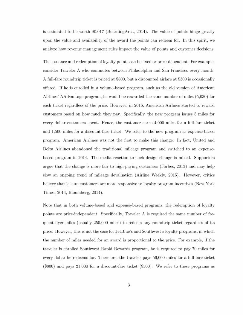
is estimated to be worth $0.017 (BoardingArea, 2014). The value of points hinge greatly

upon the value and availability of the award the points can redeem for. In this spirit, we

analyze how revenue management rules impact the value of points and customer decisions.

The issuance and redemption of loyalty points can be fixed or price-dependent. For example,

consider Traveler A who commutes between Philadelphia and San Francisco every month.

A full-fare roundtrip ticket is priced at $800, but a discounted airfare at $300 is occasionally

offered. If he is enrolled in a volume-based program, such as the old version of American

Airlines’ AAdvantage program, he would be rewarded the same number of miles (5,030) for

each ticket regardless of the price. However, in 2016, American Airlines started to reward

customers based on how much they pay. Specifically, the new program issues 5 miles for

every dollar customers spent. Hence, the customer earns 4,000 miles for a full-fare ticket

and 1,500 miles for a discount-fare ticket. We refer to the new program as expense-based

program. American Airlines was not the first to make this change. In fact, United and

Delta Airlines abandoned the traditional mileage program and switched to an expense-

based program in 2014. The media reaction to such design change is mixed. Supporters

argue that the change is more fair to high-paying customers (Forbes, 2013) and may help

slow an ongoing trend of mileage devaluation (Airline Weekly, 2015). However, critics

believe that leisure customers are more responsive to loyalty program incentives (New York

Times, 2014, Bloomberg, 2014).

Note that in both volume-based and expense-based programs, the redemption of loyalty

points are price-independent. Specifically, Traveler A is required the same number of fre-

quent flyer miles (usually 250,000 miles) to redeem any roundtrip ticket regardless of its

price. However, this is not the case for JetBlue’s and Southwest’s loyalty programs, in which

the number of miles needed for an award is proportional to the price. For example, if the

traveler is enrolled Southwest Rapid Rewards program, he is required to pay 70 miles for

every dollar he redeems for. Therefore, the traveler pays 56,000 miles for a full-fare ticket

($800) and pays 21,000 for a discount-fare ticket ($300). We refer to these programs as

3

point-based programs.

This paper aims to study the interaction between revenue management and loyalty pro-

grams. Specifically, we focus on the following three questions.

1. How to characterize revenue management decisions in the presence of loyalty pro-

grams?

2. How should firms determine the amount of capacity to set aside for loyalty awards?

3. What are pros and cons of each type of loyalty programs?

To answer these questions, we gathered empirical evidence from participants about their

perceptions of loyalty programs. Based on the evidence, we incorporate loyalty programs

into Littlewood’s (1972) model of quantity-based revenue management. In the classic model,

the firm sells a limited capacity by allocating it between low-paying customers already

seeking to buy and high-paying customers who may not arrive; in our model, we add

loyalty awards as a third use of the firm’s capacity. Customers choose between paying cash

and redeeming awards to maximize utility. We solve for the customers’ medium of purchase

and the firm’s revenue management decisions in equilibrium under three different program

designs. We have three conclusions.

First, we show that revenue management algorithms need to be adjusted by including award

liability into prices. The award liability reflects the expected opportunity cost of fulfilling fu-

ture redemptions of loyalty points. Nevertheless, this adjustment becomes redundant when

the issuance of points is proportional to prices (expense-based and point-based schemes). In

such cases, revenue management decisions are prescribed as if there is no loyalty programs.

Second, the optimal award capacity is constrained by quantity sold to customers. The reason

is that the firm needs to restrict the redemption probability of loyalty points and limit their

values, so that the customers prefer to use points immediately rather than hoard them for

future use, since “future use” may never materialize. However, if the number of redeemed

4

points is proportional to the price (point-based schemes), a 100% award availability rate

can be optimal, which can be explained below. The specific redemption rule creates a fixed

conversion rate between cash and point. On the demand side, customers have no incentives

to hoard points for future uses. On the supply side, the firm can treat award customers and

cash-paying customers equally, and provide an award availability rate as high as 100%.

Finally, we compare the three types of program schemes. Volume-based schemes enhance

profits but generate accounting challenges; expense-based programs maintain profitability

while eliminating accounting challenges; point-based programs give up these profits in return

for customer satisfaction with a 100% award availability. As explained in the previous point,

a low redemption probability induces customers to spend loyalty points more immediately.

In fact, customers spend more than they are willing to pay in cash. Consequently, when

giving out loyalty awards and collecting payment in the form of loyalty points, the firm

can extract a higher payment than what could have been possible with cash. In contrast,

point-based programs create a fixed conversion rate between points and cash, which does

not breed overspending behavior of loyalty points. Hence, point-based programs are less

profitable but also less restrictive - firms need not maintain a low redemption probability

and find it optimal to accept any redemption requests.

1.2. Literature Review

There has been extensive research on loyalty programs in the marketing literature. Readers

can refer to Bijmolt et al. (2010) and Breugelmans et al. (2014) for recent reviews. This

body of work seeks to measure the effect of loyalty programs using sales data and results

are mixed. Early studies (e.g., Sharp and Sharp, 1997) did not find significant evidence

of increased purchase frequency. There were also results suggesting that loyalty programs,

even if profitable, do not derive benefit from frequent buyers: loyalty programs have the

least impact on these customers (Lal and Bell, 2003), and yet they are the ones most

likely to claim rewards (Liu, 2007). However, Bolton et al. (2000) showed that members

of loyalty programs discount or overlook negative service experiences. In another study,

5

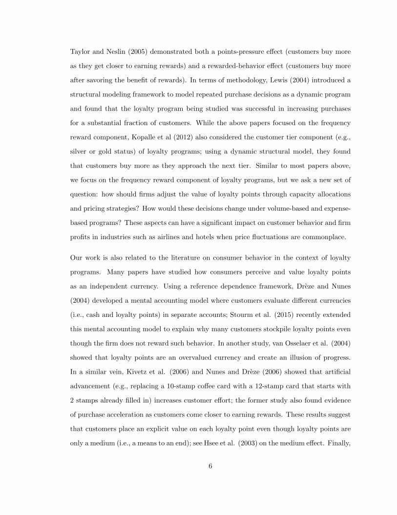
Taylor and Neslin (2005) demonstrated both a points-pressure effect (customers buy more

as they get closer to earning rewards) and a rewarded-behavior effect (customers buy more

after savoring the benefit of rewards). In terms of methodology, Lewis (2004) introduced a

structural modeling framework to model repeated purchase decisions as a dynamic program

and found that the loyalty program being studied was successful in increasing purchases

for a substantial fraction of customers. While the above papers focused on the frequency

reward component, Kopalle et al (2012) also considered the customer tier component (e.g.,

silver or gold status) of loyalty programs; using a dynamic structural model, they found

that customers buy more as they approach the next tier. Similar to most papers above,

we focus on the frequency reward component of loyalty programs, but we ask a new set of

question: how should firms adjust the value of loyalty points through capacity allocations

and pricing strategies? How would these decisions change under volume-based and expense-

based programs? These aspects can have a significant impact on customer behavior and firm

profits in industries such as airlines and hotels when price fluctuations are commonplace.

Our work is also related to the literature on consumer behavior in the context of loyalty

programs. Many papers have studied how consumers perceive and value loyalty points

as an independent currency. Using a reference dependence framework, Dreze and Nunes

(2004) developed a mental accounting model where customers evaluate different currencies

(i.e., cash and loyalty points) in separate accounts; Stourm et al. (2015) recently extended

this mental accounting model to explain why many customers stockpile loyalty points even

though the firm does not reward such behavior. In another study, van Osselaer et al. (2004)

showed that loyalty points are an overvalued currency and create an illusion of progress.

In a similar vein, Kivetz et al. (2006) and Nunes and Dreze (2006) showed that artificial

advancement (e.g., replacing a 10-stamp coffee card with a 12-stamp card that starts with

2 stamps already filled in) increases customer effort; the former study also found evidence

of purchase acceleration as customers come closer to earning rewards. These results suggest

that customers place an explicit value on each loyalty point even though loyalty points are

only a medium (i.e., a means to an end); see Hsee et al. (2003) on the medium effect. Finally,

6

Raghubir and Srivastava (2002) and Wertenbroch et al. (2007) found that consumers’

valuation of an unfamiliar currency (such as loyalty points) is biased towards the face value;

a possible explanation is that consumers anchor on the nominal face value and do not adjust

sufficiently for the exchange rate when making decisions. Sayman and Hoch (2014) showed

that buyers are willing to pay a price premium for loyalty points, and the premium is less

than the normative levels. Motivated by these behavioral studies, our theoretical model

takes the view that each loyalty point is a unit of currency valued at the nominal face value

of goods that it can be redeemed for.

It is useful to put our work in the context of existing research that elucidates the economic

function of loyalty programs. The bulk of this research focuses on the switching costs

generated by loyalty programs (for example, travelers who have accumulated many miles

at an airline will not be keen to switch to another airline). Consequently, loyalty programs

soften price competition and facilitate tacit collusion; see Kim et al. (2001), Singh at al.

(2008) and Fong and Liu (2011) for models along these lines. Another economic explanation

for loyalty programs is price discrimination. Since frequency rewards such as buy-n-get-one-

free are a type of quantity discounts, loyalty programs can facilitate price discrimination

between frequent and occasional customers (Hartmann and Viard, 2008), or between “cherry

pickers” who buy from lowest-priced stores and single-store-shoppers (Lal and Bell, 2003),

or between heavy and light users (Kim at al, 2001). Next, it has also been demonstrated

that loyalty programs enable firms to profit from the agency relationship between employers

and employees. Typically, employers pay for business trips but employees reap the benefits

from loyalty rewards; see Cairns and Galbraith (1990) and Basso et al. (2009). In another

study, Kim et al. (2004) showed that loyalty programs can help regulate capacity in face of

demand uncertainty: when demand is low, firms can offer loyalty rewards to reduce excess

capacity and ease the pressure to slash prices. Although we have limited capacity in our

model, our results do not rely on this mechanism because in our model, capacity is allocated

for redemption before demand uncertainty is realized. Instead, our analysis highlights a new

function of loyalty programs: since loyalty points are appraised at face value, they enable

7

firms to extract surplus when customers redeem points on items that they are unwilling to

pay cash to buy.

Another stream of related literature is the revenue management literature on capacity con-

trols. In most models, the firms allocates capacity to different booking classes, and when

a lower-priced booking class is sold out, customers can only purchase at a higher-priced

booking class. Such capacity allocation decisions trace back to Littlewood (1972), who

showed using a two-class model that current bookings should be accepted as long as their

revenue exceed the expected value of future bookings. This work has been extended to

multiple booking classes (e.g., Wollmer, 1992, Brumelle and McGill, 1993, Robinson, 1995)

in arbitrary order of arrival (e.g., Lee and Hersh, 1993, Lautenbacher and Stidham, 1999).

Now known as Littlewood’s rule, the original model has also been the basis for the expected

marginal seat revenue heuristics, which were proposed by Belobaba (1989) and widely used

in revenue management practice (see comprehensive reviews by McGill and van Ryzin, 1999,

Bitran and Caldentey, 2003, Elmaghraby and Keskinocak, 2003, and the reference book by

Talluri and van Ryzin, 2004). Subsequent revenue management models of capacity controls

incorporate additional complexities such as buy-up behavior (Belobaba and Weatherford,

1996), customer substitution (Shumsky and Zhang, 2004), choice between parallel flights

(Zhang and Cooper, 2005), and competition (Netessine and Shumsky, 2005). Our analysis

in this paper is based on Littlewood’s rule, but our research takes a different perspective:

instead of allocating capacity to lower-priced classes, we are interested in allocating capac-

ity for redemption of loyalty rewards. In fact, given that this is a central concern in any

capacity-constrained firm running a loyalty program, we are surprised that there has been

little to no work on understanding the interactions between capacity and loyalty rewards.

More recently, over the last decade, the literature on revenue management and dynamic

pricing has paid more attention to strategic customer behavior (see Netessine and Tang,

2009, for a review). When making purchase decisions, customers adopt a forward-looking

perspective and take future price changes and potential stock-outs into consideration (see,

8

e.g., Su, 2007, Liu and van Ryzin, 2008, Aviv and Pazgal, 2008). Such a dynamic customer

perspective is particularly important in the context of loyalty programs because frequency

rewards earned over multiple purchases are inherently dynamic. In our model, not all loy-

alty points will be redeemed and capacity may not always be available for redemption;

such factors influence the value of loyalty points and are incorporated using modeling ap-

proaches in Su and Zhang (2008) and Cachon and Swinney (2009). The literature has also

studied consumer stockpiling of purchases (Su, 2010, Besbes and Lobel, 2015), which may

be relevant for accumulation of loyalty points, but we do not consider stockpiling in this

paper.

Recently, we are thrilled to see a few papers in the operations literature on the optimal

design of loyalty programs. Sun and Zhang (2015) examine the expiration terms of cus-

tomer reward programs and find that a finite expiration term can increase firm profits, even

without accelerating consumer purchases. Our model does not specify the expiration terms,

so it applies to the airline and hotel industry where unused points can rollover. Chun and

Ovchinnikov (2015) study the customer tier component of loyalty programs (eg, require-

ments to reach gold status), while we focus on the frequency reward component of loyalty

programs (eg, requirements for a free flight). Methodologically, to capture customers’ inter-

temporal decisions, Sun and Zhang (2015) develop a full dynamic programming model,

while Chun and Ovchinnikov(2015) allow customers to choose how many flight to fly over

a year. In contrast, our model simplifies the decision dynamics by incorporating the value

of the loyalty program currency, which is endogenously determined by firm and customers’

strategic behavior.

1.3. Behavioral Evidence of Consumer Model

Fundamentally, loyalty programs create a new option for customers: buying with points.

The starting point for any model-building activity is to understand how customers perceive

this option. Consider a customer who is eligible to redeem for an award. The first question

we address here is to find the plausible model for his redemption behavior.

9

At the most basic level, the model will involve (at least) a binary choice between buying

with cash (pay the current price) and buying with points (pay the loyalty points). The goal

of this section is to establish the boundary of a plausible model for that binary decision.

Consider a customer who makes the binary decision: cash or points. It is clear that the

customer chooses to pay points when the current cash price is high and vice versa. Hence,

there is a maximum price that he will pay to keep his points. This maximum price can be

seen as a proxy for the customer’s “value of points”. Note that if the customer chooses to

pay the maximum price, he automatically hoards the points for future purchases. Hence,

the “value of points” hinges on their future purchasing power. The question is how the

customer determines this “purchasing power”. Specifically, we ask the following questions.

What are the metrics the customers rely on for the evaluation of the “purchasing power”?

Is the “purchasing power” determined dynamically or one-shot? In the rest of this section,

we shall discuss each of the two questions separately.

First, intuitively, the “purchasing power of points” should be dependent on the customer’s

expectation about the future prices that these points can redeem for. In fact, there is ample

evidence in the literature supporting this theory. Thaler (1985) proposes that consumers

consider not only the benefits from the good they might buy but also the perceived merits

of the deal: whether the actual price is higher or lower than they expect. Take the airline

industry for example. When travelers decide the time to redeem their frequent flyer miles,

they are not only concerned about the benefit and convenience generated from the flight

ticket, but also whether the purchase is a “good bargain”. In Thaler’s study, participants

imagined sitting on a beach with a friend who had just offered to bring them back a

bottle of their favorite beer. When told that beer would be purchased from a fancy hotel,

participants authorized their friend to spend $2.65, but when told the retailer was a run-

down grocery store, they were willing to pay just $1.50. In other words, the expectation

to pay became the willingness to pay, i.e. the customer’s maximum price to keep the

beer is linked to his expectation to pay in that store.This is referred to as the Reference

10

Price Theory (Weaver and Frederick, 2012). In the context of airlines, it is likely that the

customer’s maximum price to keep the points are linked to the customer’s expectation to

pay for a future redeemable flight ticket. If this is true, the effect of expectation (reference

price) should be reflected in customers’ behavior: when the expectation of future prices is

higher, points become more worthy and the maximum price customers pay to keep points

is higher.

Second, the value of points may be determined either dynamically or one-shot. If it is

determined dynamically, it must be state-dependent, i.e. the value of points varies with how

many points the customer has already accumulated. Otherwise, it is state-independent. We

shall discuss each case separately. In our previous airline example, a customer trying to

redeem frequent flyer miles must be aware of the potential trips that he can accumulate

miles from or redeem miles for in the future, and have rational beliefs about their future

utilities and market prices in advance. To fully capture this process, a dynamic program

over multiple periods is required. In each period, the customer may incur a need to take a

flight. In this dynamic program, the customers’ state variable is the amount of miles they

accumulated in their frequent flyer account, and their decision variable is whether to redeem

the miles or pay cash for each trip. Even if a full-fledged dynamic program is implausible, as

long as there is any dynamic consideration (even if imperfectly so), there will be some state

dependence, and decisions will depend on mileage balance. Intuitively, it is quite obvious

that with a higher mileage balance, the customer is more likely to use miles more freely.

On the other hand, evidence suggests that some customers may view the evaluation of points

as a one-shot decision. Specifically, many frequent flyers follow a simple rule of thumb: they

form an implicit estimation of the average value of one mile, and conclude that it is a good

deal to use miles when the value of a mile given the current price exceeds the average value

of a mile. For example, Tripadvisor.com calculated that each mile is worth ¢1.4. This

was derived from dividing the average domestic roundtrip ticket price $350 by the required

25,000 miles. Using this baseline, customers can calculate whether any ticket is worth using

11

the miles for. A frequent flyer (Smarttravel) has the following examples: “Cashing in 25,000

miles for a ticket that could be purchased for $100 yields just ¢0.4. On the other hand,

redeeming 100,000 miles for a business-class ticket to Europe priced at almost $11,000 yields

a nominal per-mile value of ¢11, slightly less with the hassle factor adjustment.” Following

this rule of thumb, a customer should purchase the $100 ticket in cash and the $11,000

ticket in miles. Some frequent flyers have developed online spreadsheets to calculate when

to redeem miles, while the exact baseline can be adjusted to different airlines, programs,

or even the customers’ own calibration. Instead of evaluating miles dynamically, customers

stick to a fixed value of miles when making the binary decision. Nevertheless, they are

still strategic in the sense that they balance the tradeoff between using the miles right

away (which gives a value of ¢0.4 cent and ¢11 cents per mile in the previous examples

respectively), and hoarding the miles for later use (which yields an expected value of ¢1.4

per mile). Note that the Tripadvisor.com example not only supports the one-shot evaluation

hypothesis, but also echoes the reference theory: the evaluation of points depends on the

average price $350 of a flight ticket, which sets customers’ expectation of the future price.

Both the “reference price” theory and the “dynamic vs one-shot” hypotheses are plausible,

we need to run a study. In the study, we shall test whether the customers’ redemption

decisions are price-dependent (reference theory) and state-dependent (dynamic vs one-shot).

Experiment Design Participants (N = 510) were recruited on Amazon Mechanical Turk.

They were asked to complete a survey. In the beginning of the survey, they answered the

screening question whether they are members of any frequent flyer programs. Then they

considered the hypothetical situation to choose a flight destination that they would like to

redeem using miles. They were first told the following: “Imagine that you have accumulated

enough miles for a free round-trip flight anywhere in the continental US. Where is your

most likely destination?” Choosing the destination initially pins down the flight before any

manipulations come in.

They then examined the option to pay the average cash price for the chosen flight. In the

12

high (low) average price segment, participants were asked: “Next, imagine that a trusted

friend familiar with airlines tells you that the average price of a round-trip flight is $800

($300). If you did not have any miles, are you willing to pay $800 ($300) for this flight?”

Finally, they examined the options between paying cash and redeeming miles for the flight.

They were given information about their mileage balance (200,000 or 50,000), the average

price of the redeemable flight ($800 or $300 as in the previous question), and the current

price (ranging from $0 to $1000 with increment of $100), which might differ from the average

price. In the high (low) average price/mileage balance group, participants are asked “You

have 200,000 (50,000) miles in your account and you can use 25,000 miles to pay for the

flight. The average price for the flight is $800 ($300) but the actual price you find might

be higher or lower. At each price below, do you prefer to pay money or use miles?” The

participants then chose from a list of current prices and identified the maximum price they

would like to pay to keep their miles, i.e. their willingness to pay for the miles (WTP).

Specifically, the midpoint of the two prices where the customer switched from “money” to

“miles” is used to calculate WTP.

Therefore, the experiment should be able to answer the following question related to the

binary decision: whether it is state-dependent and subject to reference-price effects.

Results We restrict our analysis on 244 participants who responded that they were en-

rolled in some frequent flyer programs. These participants have had previous experience

with the accumulation and redemption of loyalty points and their behavior will most reflect

the loyalty program members’ decisions in practice. The key statistics are summarized in

Table 1:

13

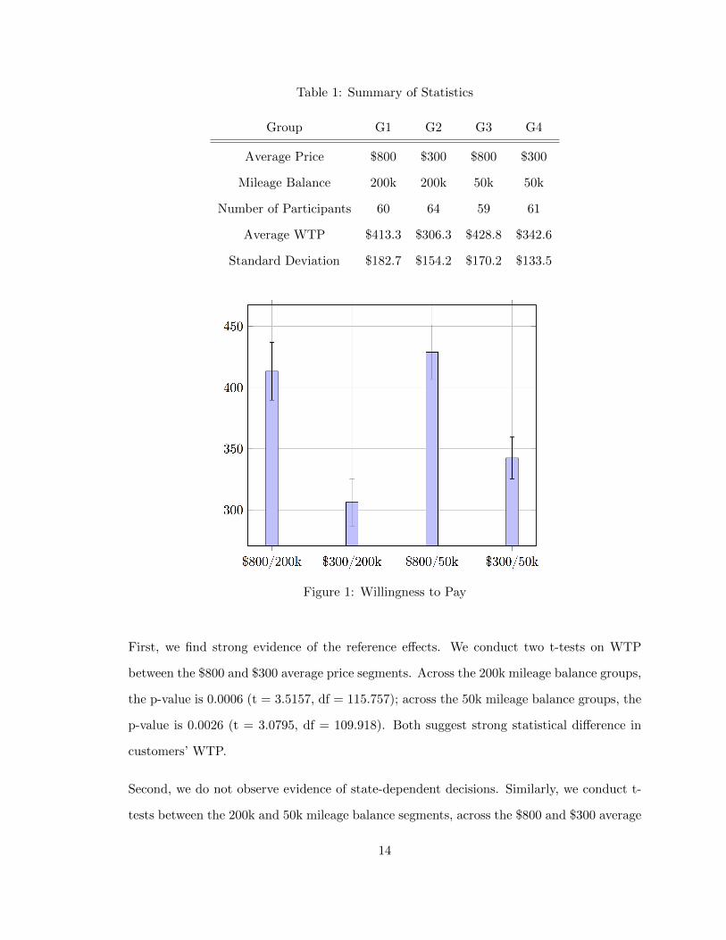
Table 1: Summary of Statistics

Group G1 G2 G3 G4

Average Price $800 $300 $800 $300

Mileage Balance 200k 200k 50k 50k

Number of Participants 60 64 59 61

Average WTP $413.3 $306.3 $428.8 $342.6

Standard Deviation $182.7 $154.2 $170.2 $133.5

Figure 1: Willingness to Pay

First, we find strong evidence of the reference effects. We conduct two t-tests on WTP

between the $800 and $300 average price segments. Across the 200k mileage balance groups,

the p-value is 0.0006 (t = 3.5157, df = 115.757); across the 50k mileage balance groups, the

p-value is 0.0026 (t = 3.0795, df = 109.918). Both suggest strong statistical difference in

customers’ WTP.

Second, we do not observe evidence of state-dependent decisions. Similarly, we conduct t-

tests between the 200k and 50k mileage balance segments, across the $800 and $300 average

14

price groups separately. The p-values are 0.6333 (t = -0.4783, df = 116.665) and 0.1605 (t

= -1.412, df = 121.897), showing no significant effects of mileage balances.

Finally, we run a regression with all demographic information controlled (gender, age, fre-

quent flyer program, true mileage balance, travel frequency, etc.). The effect of average

price on WTP is significant (p=6.62e-06); by increasing the average price from $300 to

$800, the WTP increased by $97.453. However, the effect of mileage balance is not statis-

tically significant (p=0.1058).

Consumer Behavior Model Based on the evidence, we need to incorporate the follow-

ing properties of consumer decisions when building a coherent model: i) consumers evaluate

points in a one-shot manner; ii) consumers evaluate points according to their expectations

of future prices. We shall describe the consumer behavioral model briefly below.

Consider a loyalty program member i who has accumulated enough points to redeem a free

unit that he evaluates at vi. He chooses between the following three options: i) pay the

current cash price p and earn N points (I); ii) use M points to redeem for a free unit (A);

iii) leave the market (O).

The customer then evaluates points as a one-shot decision. We shall use w as the value of

a point. Then the customer’s utility from a purchase is

u(I) = vi +Nw − p,

from a redemption is

u(A) = vi −Mw,

from leaving the market is exactly 0. The customer compares these three options and

determines a preference rule denoted by ai.

Finally, we describe how the value of loyalty points w depends on the firm’s and customers’

decisions. The empirical study suggests strong effect of reference price, i.e. customers

15

evaluate points according to the average price of an award. We will incorporate that into

our model. Specifically, We characterize the market value of a point as

w =R · σM

,

where R is the market value of an award unit, σ is the probability that each point will

eventually be redeemed, and M is the number of miles required for an award. The market

value R is the net price at the time of redemption: i.e., if the prevailing price at the time

of redemption is p, then the market value of the award unit is p − Nw; we subtract Nw

where N is the average number of points issued to customers with a cash-paid purchase.

The setup is consistent with the reference price (p) effects. The redemption probability σ

is simply the ratio of the average number of redeemed points over the average number of

issued points. (For example, if an airline issues twice as many miles as are redeemed, then

the chances that each mile will be redeemed is 50% on average.)

Note that the value R depends on the firm’s pricing decisions, while the value σ depends

on the firm’s award capacity decisions. Hence, the value of a point w is endogenous. In the

next section, we will describe the firm’s model in detail.

1.4. Firm’s Model and Equilibrium

Our model builds on Littlewood’s (1972) model of quantity-based revenue management.

In the classic model, there is a firm that sells a fixed capacity of K units over two time

periods. In period one, the firm faces an infinite population of low-type customers, each

with valuation vL for a unit of capacity. In period two, the firm faces a random population

of X ∼ F (·) high-type customers, each with valuation vH , where vH > vL. The firm sells

qL units to low-types and reserves qH units for high-types, where qL + qH = K. Given the

decision above, the expected profit is vL ·qL+vH ·E[qH ∧X], which demonstrates a tradeoff

between the guaranteed but lower revenue from low-types and the higher but uncertain

revenue from high-types. The profit-maximizing decision, known as Littlewood’s rule, is

16

q0H = min{K, q}, where q = F−1( vLvH ). We use q0

H , q0L, π

0 to denote the optimal decisions

and profit in the classic model.

Loyalty Program Now, we introduce loyalty programs into Littlewood’s setting. Assume

that with loyalty programs, the firm charges prices pL and pH to low and high types. For

each unit purchased at pi, the firm issues Ni loyalty points to the customer; once a customer

accumulates Mi points, the customer may redeem those points for a free unit priced at pi,

i = L,H.

This general setup is applicable to the three types of loyalty programs of interest: volume-

based programs, expense-based programs, and point-based programs. For example, in a

volume-based program (old AAdvantage) that issues 5,030 miles for a round-trip US coast-

to-coast flight and requires 25,000 miles for a free flight, we have NL = NH = 5, 030 and

ML = MH = 25, 000. In an expense-based program (new AAdvantage) that issues 5 miles

for every dollar spent by a customer and requires 25,000 miles for a free flight, we have

Ni = 5 · pi, i = L,H and ML = MH = 25, 000. In a point-based program (Southwest Rapid

Rewards) that issues 6 miles for every dollar spent by a customer and requires 70 miles for

every dollar redeemed by a customer, we have Ni = 6 · pi and Mi = 70 · pi, i = L,H.

We consider a setting where the firm sells the same capacity of K units repeatedly over time.

In the airline example, miles earned on a current flight may be redeemed for a future flight.

Nonetheless, each individual flight is managed similarly to the classic model as described

below.

Firm Decisions With loyalty programs, the firm divides the capacity of K units into

three instead of two pools. As before, the firm chooses a protection level qH (number of

units to reserve for high-types) and a booking limit qL (number of units to sell to low-types),

but now the firm also sets aside qA units for award redemption. We use q = (qA, qL, qH) to

denote the capacity allocation decision, where the three components are nonnegative and

add up to K. In addition, the firm chooses prices pL and pH to charge to low and high

17

types, and we denote p = (pL, pH). The firm’s objective, as before, is to maximize total

expected profit.

Profit Function Having specified the firm’s decisions (p, q) and customers’ preference

rules a = (aL, aH), we are now ready to write down the profit function:

π(p, q, a) = pL · sL(q, a) + pH · sH(q, a),

where sL and sH denote the expected number of units sold at the two prices. The former

is sL = qL if low-types buy and zero otherwise. The latter is sH = E[qH ∧X] if high-types

buy before redemption, sH = E[qH ∧ (X − qA)+] if high-types buy after redemption, and

zero otherwise. Finally, we also use sA(q, a) to denote the expected number of award units

redeemed, even though they do not contribute to revenue and thus do not enter the profit

function directly. There are four possible values for sA: if no customers redeem, sA = 0; if

low types redeem, sA = qA; if high types redeem as their first choice, sA = E[qA ∧ X]; if

high types redeem after purchases, sA = E[qA ∧ (X − qH)+]. Given sL, sH and sA, we can

express the redemption probability as follows

σ(p, q, a) =MsA

NLsL +NHsH,

as before, M is the average number of points charged for a redemption.

Timeline and Equilibrium The chronology of events is as follows. First, the firm

chooses a revenue management strategy (p, q), which is observed by all. Then, low-types

arrive and choose their preference rule aL; this is followed by sales to and/or redemptions

by low-types, after which they leave the market. Finally, high-type demand X is realized,

they observe the entire history and choose their preference rule aH , and then sales to and

redemptions by high-types occur. Given this timeline, we use backward induction to solve

for the sub-game perfect equilibria, which can be defined as follows.

18

Definition An equilibrium (p∗, q∗, a∗) satisfies the following conditions.

1. (Customer optimality) Given any (p, q), customers choose a∗(p, q) to maximize utility.

2. (Firm optimality) The firm chooses (p∗, q∗) to maximize expected profit:

p∗, q∗ = arg maxπ(p, q, a∗(p, q)) (1)

1.5. Volume-Based Loyalty Programs

We first consider volume-based programs. In such programs, the firm issues the same num-

ber of points to each purchase and requires the same number of points for each redemption,

regardless of the prices. For simplicity, we shall denote N = NL = NH and M = ML = MH .

By solving the customers’ and firm’s problems, we characterize the equilibrium below.

Proposition 1. In the equilibrium,

(i) Low types buy q∗L, then redeem q∗A; high types buy q∗H .

(ii) p∗i = vi +Nw∗;

(iii) There exists K such that

(a) if K ≤ K, then q∗L = 0 and q∗A, q∗H satisfy

q∗A + q∗H = K, q∗A =σ∗N

ME[q∗H ∧X].

(b) If K > K, then q∗H = q and q∗A, q∗L satisfy

q∗A + q∗L + q = K, q∗A =σ∗N

M{q∗L + E[q ∧X]}.

Here, q = F−1(p∗L−cp∗H−c

) and c = σ∗NM+σ∗N pL.

19

(iv) The equilibrium profit is vL · q∗L + vH · q∗A + vH · E[q∗H ∧X].

(v) R∗ = vH , σ∗ = vLvH

, w∗ = vLM .

Proposition 1(i) summarizes equilibrium customer behavior (Figure 1). First, low types

prefer to pay the low price but are willing to redeem awards when the low-price capacity

runs out; this is intuitive because at sufficiently low prices, customers would seize the deal

and save points for future use. Second, high types are willing to pay the high price. Hence,

the following sequence of events occur in equilibrium: 1) upon arrival, low types purchase

at the low price pL; 2) low-price capacity qL runs out, so the prevailing price rises to pH ; 3)

low types who have not received a unit redeem awards using their points; 4) award capacity

qA runs out, 5) all remaining low types leave the market; 6) high types arrive and buy at the

high price. Given this chronology, the prevailing price is the high price when redemptions

occur, so it is not surprising that the market value of awards is R∗ = vH as indicated in

Proposition 1(iv).

Figure 2: Equilibrium Timeline

Next, we discuss the firm’s equilibrium decisions. As shown in Proposition 1(ii), the firm

selects prices p∗i = vi + Nw∗ to extract maximum customer surplus. The prices consist of

two parts: the value of the unit (vi) and the value of issued points (Nw∗). With these prices,

Proposition 1(iii) then summarizes the equilibrium capacity allocation q∗. To understand

20

this result, we first introduce a critical fractile q. We can rewrite the equation of q as follows:

(p∗H − c)F (q) = p∗L − c.

This is similar to the critical fractile q used in Littlewood’s rule in our baseline model: the

left hand side is the expected revenue from reserving an additional unit for the high type

customers; the right hand side is the certain revenue from giving this unit to the low types.

However, there is an additional cost c associated with the revenues. This is the cost of

issuing points. For each unit sold, the firm issues N points, each of which is redeemed with

probability σ∗ for 1M unit of capacity. In other words, each sold unit is associated with the

liability of fulfilling σ∗NM units worth of loyalty rewards. Altogether, the firm needs a total

of 1 + σ∗NM units to sell to and award the customer, and the awarded capacity is a fraction

σ∗NM+σ∗N of this total capacity. For each unit of awarded capacity, there is an opportunity

cost of p∗L: if this unit is not awarded, then it can be sold to a low type customer at price

p∗L. Hence, the liability of issuing points is c = σ∗NM+σ∗N p

∗L.

Using the critical fractile q, we can interpret the optimal capacity allocation q∗ in Propo-

sition 1. The critical fractile q can be viewed as a protection level for high-type demand.

Protecting q units for high-types generates a total of NE[q ∧X] points and a correspond-

ing award liability of σ∗NM E[q ∧X] units. If the award liability exceeds remaining capacity

K − q, as in case (i), the firm does not sell at the low price (i.e., q∗L = 0) and lowers the

protection level q∗H below q so that the corresponding award liability can be covered by

available capacity K. In case (ii), the protection level q∗H = q and the corresponding award

liability do not take up the entire capacity K. Then, the remaining capacity is allocated

to low-price capacity q∗L and the corresponding award liability σ∗NM q∗L. In other words, we

have q∗L + σ∗NM q∗L + q + σ∗N

M E[q ∧X] = K, as indicated in the proposition.

Finally, Proposition 1(iv) gives the equilibrium profit, which is similar to the expected

profit vL · q∗L + vH ·E[q∗H ∧X] in the classic model, but has an additional term vH · q∗A. This

additional term suggests that the firm receives vH from each redeemed unit. Even though

21

the firm does not receive revenue from award redemptions, it can charge a price premium

for issuing loyalty points. When the price premium is accounted for, it is as if the firm sells

award units at the high-type valuation vH to low-type customers. In other words, when low

types redeem awards, the firm effectively uses its loyalty program to extract the high-type

valuation vH from these low-type customers. This follows directly from the reference effects:

low types refer the value of points according to the price at the redemption.

This result echoes the current accounting protocols of loyalty programs. Under the “De-

ferred Revenue” accounting criterion, firms are required to defer the revenue associated

with issued points to the point of redemption. The most prevailing way of calculating the

deferred revenue is by the “fare value” of the redeemable reward, i.e., the price at which the

award is redeemed. Put it in a simple way, the firm recognizes a revenue equivalent to the

current price at the redemption point, and this revenue must have been be deducted/de-

ferred previously at the time of issuing these points. This is exactly what Proposition 1(iv)

indicates: instead of recognizing the whole revenue pi when selling qi and 0 for rewarding

qA, the firm can record vi for qi, recognize an additional revenue for qA, and yield the same

total revenue.

To induce these low types to redeem points, Proposition 1(v) ensures that the redemption

probability is below a limit vLvH

, i.e., the chances that points can eventually be used are low

enough that low types are better off redeeming instead of hoarding them. Ultimately, the

constraint in (2) determines the amount of capacity the firm should reserve for awards: qA

should be increased to the point where the redemption rate reaches the upper limit.

In summary, loyalty programs enhance profits by extracting high revenues from low types.

The revenue management strategy must be adjusted to account for the cost and benefit of

issuing points. Specifically, the redemption probability under the optimal revenue manage-

ment strategy has to be low to prevent customers from hoarding points for future use.

22

1.6. Expense-Based Loyalty Programs

The previous section investigates volume-based loyalty programs, under which customers

receive the same number of points from each purchase, no matter how much they pay.

In practice, some companies use expense-based programs, under which customers receive

points based on the amount of money they spend. This section extends our results to

expense-based programs.

Consider American Airlines that provides an expense-based loyalty program: it issues 5

miles for each dollar spent and requires 25,000 miles for a free flight. Then, the total

number of points issued per unit depends on the price paid. For instance, a customer gets

4,000 miles for a ticket priced at $800, but only gets 1,500 miles for a ticket discounted

to $300 on the same flight. Let n be the number of points issued per dollar spent; here,

n = 5. As before, we use M to denote the number of points required for a free unit; in our

example, M = 25, 000, so customers are entitled to a free flight after spending $5,000 (e.g.,

7 full-fare flights or 17 discounted flights). This results in Ni = npi and Mi = M , where

i = L,H.

With expense-based loyalty programs, most of our results remain unchanged. We begin

with the following proposition.


(i) Low types buy q∗L, then redeem q∗A; high types buy q∗H .

(ii) p∗i = vi1−nw∗ ;


(a) if K ≤ K, then q∗L = 0 and q∗A, q∗H satisfy

q∗A + q∗H = K, q∗A =σ∗np∗HM

E[q∗H ∧X].

23


q∗A + q∗L + q = K, q∗A =σ∗np∗LM

q∗L +σ∗np∗HM

E[q ∧X].

Here, q = F−1( vLvH ).

(iv) The equilibrium profit is vL · q∗L + vH · q∗A + vH · E[q∗H ∧X];

(v) R∗ = vH , σ∗ = vLvH

, w∗ = vLM .

A quick glance at Proposition 2 reveals several similarities to Proposition 1. First, Proposi-

tion 2(i) shows that with expense-based programs, it remains optimal to induce low-types to

buy before redeeming, resulting in awards being valued at the high valuation, i.e., R∗ = vH ,

as in volume-based programs. Second, the profit function in Proposition 2(iv) remains un-

changed and shows that, by extracting a price premium for loyalty points, the firm again

receives vH from each of the qA redeemed units. In other words, whether they are volume-

based or expense-based, loyalty programs enable the firm to extract the high valuation

from each unit redeemed by a low-type. Finally, Proposition 2(v) shows that the redemp-

tion probability σ∗ = vLvH

and the value of loyalty points w∗ = vLM match our earlier results

for volume-based programs.

However, there are a couple of differences between Proposition 1 and Proposition 2. First,

to extract all consumer surplus, the firm chooses p∗i = vi + np∗iw, which gives p∗i = vi1−nw∗ .

As a result, the price premium for loyalty points enters as a multiplicative factor 11−nw∗

in expense-based programs, instead of an additive term Nw∗ in volume-based programs.

Second, the exact form of revenue management decisions differ from volume-based programs.

Nevertheless, the optimal capacity allocation rule for expense-based programs follows the

same logic as before. We start with a protection level q for high-types, a la Littlewood. If

this protection level and the associated award liability exceeds capacity, then all units are

priced high and the protection level is adjusted downward to meet capacity. Otherwise,

24

the firm protects q∗H = q units for high-types and additionally allocates q∗L units for sale at

the low price so that all capacity is used up, after considering all associated award liability.

Consequently, the rule of thumb described in the previous section still applies: the optimal

award capacity can be achieved by matching the redemption probability to σ∗.

One noteworthy result in Proposition 2 is that the protection level q is identical to that

in the classic model. This is because in expense-based loyalty programs, both the price

premium and the cost of issuing points are proportional to the valuation of the customer

who made the purchase. As a result, the critical fractile q determining the protection level

is simply the ratio of customer valuations, as in the classic model. This finding leads us

to our next result. The result suggests that Expense-based programs not only retains the

property of inducing low types to pay the high price, but also simplifies the calculation of

revenue management. An expense-based program protects the same number of units for

high-types as in the classic Littlewood model, suggesting that capacity allocation decisions

can be made without considering loyalty programs. The firm only needs to collect historical

information about prices to make decisions on the protection levels.

1.7. Point-Based Loyalty Programs

In the previous section, we considered price-dependent issuance of loyalty points. In this

section, we investigate price-dependent issuance and redemption in point-based programs.

In such programs, for every unit priced at pi, a cash-paying customer earns npi points,

and a point-paying customer pays mpi points, i.e., Ni = npi and Mi = mpi. Point-based

programs have been adopted by Southwest Airlines and JetBlue Airlines.


(i) Low types redeem q∗A, then buy q∗L; high types buy q∗H .

(ii) p∗i = vi1−nw∗ ;


25

(a) If K ≤ K, then q∗L = 0 and q∗A, q∗H satisfy

q∗A + q∗H = K, q∗A =σ∗n

mE[q∗H ∧X].


q∗A + q∗L + q = K, q∗A ∈ [0,n

m(q∗L +

vHvLE[q ∧X])].

Here, q = F−1( vLvH ).

(iv) The equilibrium profit is vH · q∗A + vH ·E[q∗H ∧X] if K ≤ K, is vL · q∗L + vH ·E[q∗H ∧X]

otherwise.

(v) R∗ = vH , σ∗ = vLvH

, w∗ = vLvLn+vHm

if K ≤ K; R∗ = vL, σ∗ ≤ 1, w∗ = σ∗

σ∗n+m

otherwise.

Proposition 3 reveals several unique properties of point-based programs. First, customers

always prefer redeeming awards rather than paying cash. When the number of points

needed for redemption is proportional to the cash price, there is a fixed conversion rate

between points and cash. Therefore, customers have no incentives to hoard points for

future redemptions and they will always use points whenever an award unit is available.

Second, Proposition 3(iv) suggests that the firm can only extract the high value from award

capacity when it fully closes the low price capacity. Note that low types always redeem

before purchasing. If the low price capacity is offered, when customers redeem, the prevailing

price is low and they evaluate points according to the that price. Hence, the firm cannot

extract high values from issuing points to them. On the contrary, if the low price capacity

is closed, they can only redeem at the high price and points have high values. Therefore,

only when the low price capacity is closed do redemptions eventually generate high values

for the firm.

26

Finally, Proposition 3(iii) and (v) indicate that when the firm opens up some low price

capacity, it becomes more flexible in choosing the award capacity qA. Specifically, the limit

on the redemption probability of points is extended to be as high as 100%. Previously,

in volume-based and expense-based programs, the firm needs to restrict the redemption

probability below 100% to induce immediate redemptions by customers. Now in point-

based programs, customers never hoard points for future use. As a result, the firm can

allow 100% redemption probabilities. Moreover, since now redemptions happen at the low

price, they generate exactly the same revenues as the low price capacity. Indifferent between

selling and rewarding the low types, the firm has a more flexible rewarding rule, i.e. it can

split the Littlewood booking limit K − q arbitrarily between the award capacity qA and

low price capacity qL, as long as the redemption rate is below 100%. Specifically, the 100%

redemption probability can be optimal. In such cases, the firm does not need to distinguish

between cash-paying customers and reward customers. Instead, the firm can put them in

the same booking bucket. Consequently, a customer can always redeem an award whenever

the unit of capacity can be purchased using cash. Our result is consistent with practice - the

100% availability rate is exactly what the highly-praised point-based programs of Southwest

Airlines and JetBlue Airlines are well-known of.

1.8. Numerical Examples

In this section, we will provide some numerical examples to clarify the mechanics of the

revenue management strategies. Our primary data source is Airline Origin and Destination

Survey (DB1B) conducted by Bureau of Transportation Statistics. It is a 10% sample of

airline tickets from reporting carriers. Data includes origin, destination, price and other

itinerary details of passengers transported.

27

Figure 3: Price Distribution

We select 16 routes over the third quarter of 2015 across four airlines for analysis. At

that period of time, American Airlines offers a mileage-based (volume-based) program,

both United Airlines and Delta Airlines offers an expense-based program, and Southwest

Airlines offers a point-based program. All these routes are direct flights, with a market

share of non-stop passengers greater than 70% (mostly 100%) such that competition is

rare. The following approaches are used for model calibrations: (i) the number of standard

economy class seats on the plane is used for capacity K; (ii) the first quantile price is used

to calibrate low valuation vL and third quantile price is used to calibrate high valuation vH

(See Figure 3. The two red lines corresponds to the first quantile and third quantile price.

Data suggests that the first quantile price has the highest density in the price distribution,

which may approximate a mass probability of low type customers; we understands that

such simplifications of the valuation distribution have limitations, but hope to proceed with

the numerical examples to generate insights of the theoretical model); (iii) a quarter of

the economy class seats is used for the mean of the high type demand, i.e. E[X] = K/4,

since only 25% of all passengers paid the high value price vH ; (iv) we assume X follows the

28

normal distribution, with coefficient of variation ranging from 0.5 to 2; (v) the award policy

for United and Delta is used to calibrate Ni and Mi in both the volume-based and expense-

based programs, while the award policy for Southwest is used to calibrate for point-based

programs; (vi) we use the fraction of tickets sold under $25 as the fraction of award tickets

(illustrated in blue dashed line in Figure 3), and multiply that by K for the award space

qA in practice (the tax paid for redemption ranges from $5 to $10, and the probability of

paid price between $10 and $25 is less than 1%).

Table 2 summarizes the results of the 16 routes, by calculating the optimal RM strategies

and profit improvements of loyalty programs (∆Π). The routes are listed in ascending

order of flying distance. Note that there is a pattern of increasing ∆Π of the volume-based

program and a decreasing-increasing ∆Π of the expense-based program. We will discuss

three routes in detail below.

(1) BOS - CVG (Delta): Table 2 has three implications. First, it indicates that Delta is

better off with the expense-based program for this route. Because of the high price and

short distance of the route, an expense-based program issues more miles to customers

compared to the mileage-based programs. Since each mile yields high valuations, the

airline can benefit from “selling” these miles to customers. Second, Delta Airlines

over-reward its customers under the expense-based program. While it gives 7.6 seats

to its award passengers, the optimal reward level is only around 5.8. This can be

due to the simple approximation of demand distribution. Finally, although the point-

based program does not generate higher revenues directly, it can significantly enhance

award space and potentially lead to higher customer satisfaction. (The same logic

applies to Route (2) - (6).)

(15) SFO to CLT (American): compared to Route (1), Route (15) has much longer dis-

tance. As a result, a mileage based program issues more miles to customers. For this

specific route, American Airlines benefit from its mileage-based programs more, since

putting more miles into circulation allows the firm to gain higher profits. In fact, the

29

number of capacity rewarded to customers (3.1 seats) is close to the optimal level

in the model (2.8 seats). Finally, note that although the mileage-based program is

slightly better, the expense-based program also enhances the profits over 5.7%. (The

same logic applies to Route (7) - (16).)

(9) DAL to PHL (Southwest): this is a medium-haul flight. As in the case of flight (15),

the volume-based program is more profitable. However, the point-based program

allows significantly more award space, thus Southwest is able to apply a simple rule

of thumb: treat award customers exactly the same as cash passengers. Note that the

qA in data is greater than the optimal qA under the point-based program. This may

be due to two reasons: (i) biased sample of the price distribution; (ii) the ratio of

award redemptions is relatively lower in other routes, to make up for the additional

redeemed miles in this specific route.

30

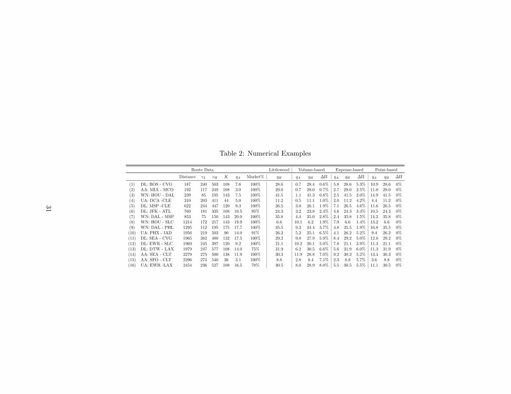
Table 2: Numerical Examples

Route Data Littlewood Volume-based Expense-based Point-based

Distance vL vH K qA Market% qH qA qH ∆Π qA qH ∆Π qA qH ∆Π

(1) DL: BOS - CVG 187 240 503 108 7.6 100% 28.6 0.7 28.4 0.6% 5.8 28.6 5.3% 10.9 28.6 0%(2) AA: MIA - MCO 192 117 249 108 3.0 100% 29.0 0.7 29.0 0.7% 2.7 29.0 2.5% 11.0 29.0 0%(3) WN: HOU - DAL 239 85 195 143 7.5 100% 41.5 1.1 41.3 0.8% 2.5 41.5 2.0% 14.9 41.5 0%(4) UA: DCA -CLE 310 203 411 44 5.0 100% 11.2 0.5 11.1 1.0% 2.0 11.2 4.2% 4.4 11.2 0%(5) DL: MSP -CLE 622 244 447 120 9.3 100% 26.5 3.0 26.1 1.9% 7.1 26.5 4.6% 11.6 26.5 0%(6) DL: JFK - ATL 760 181 335 108 10.5 95% 24.3 3.2 23.8 2.4% 4.6 24.3 3.4% 10.5 24.3 0%(7) WN: DAL - MSP 853 75 150 143 20.0 100% 35.8 4.4 35.0 2.8% 2.4 35.8 1.5% 14.2 35.8 0%(8) WN: HOU - SLC 1214 172 217 143 19.9 100% 6.6 10.1 6.2 1.9% 7.9 6.6 1.4% 13.2 6.6 0%(9) WN: DAL - PHL 1295 112 195 175 17.7 100% 35.5 9.3 34.4 3.7% 4.8 35.5 1.9% 16.8 35.5 0%(10) UA: PHX - IAD 1956 219 503 90 14.0 91% 26.2 5.2 25.1 6.5% 4.1 26.2 5.2% 9.4 26.2 0%(11) DL: SEA - CVG 1965 262 480 132 17.5 100% 29.2 9.8 27.9 5.9% 8.4 29.2 5.0% 12.8 29.2 0%(12) DL: EWR - SLC 1969 245 397 120 9.2 100% 21.1 10.2 20.1 5.0% 7.8 21.1 3.9% 11.3 21.1 0%(13) DL: DTW - LAX 1979 247 577 108 14.0 75% 31.9 6.2 30.5 6.6% 5.6 31.9 6.0% 11.3 31.9 0%(14) AA: SEA - CLT 2279 275 500 138 11.9 100% 30.3 11.9 28.8 7.0% 9.2 30.3 5.2% 13.4 30.3 0%(15) AA: SFO - CLT 2296 274 540 36 3.1 100% 8.8 2.8 8.4 7.1% 2.3 8.8 5.7% 3.6 8.8 0%(16) UA: EWR -LAX 2454 236 527 108 16.5 78% 30.5 8.0 28.9 8.0% 5.5 30.5 5.5% 11.1 30.5 0%

31

Figure 4: Profit Benefit of Loyalty Programs (Unit: %)

Finally, we plot the six high-fare routes (with a low price ranging from $240 to $274) in

Figure 4. The horizontal axis is the high price vH , and the vertical axis is the flying

distance. The contour lines indicate the percentage of profit improvement of volume-based

and expense-based programs over the classic Littlewood model. Moreover, the shaded areas

suggests that expense-based programs are more profitable than volume-based programs.

In Figure 4, as the flying distance increases or high price increases, the loyalty programs

become more profitable. This is because the firm is able to issue more miles in such scenarios.

Specifically, the volume-based program is more profitable than the expense-based when the

flying distance is longer, as for the four routes above the line. In contrast, for short-haul

expensive flights (bottom Delta routes), expense-based programs are more profitable.

32

1.9. Conclusions

In this paper, we study loyalty programs in industries such as airlines and hotels where

capacity is limited. Starting with Littlewood’s classic revenue management model with two

customer types (e.g., leisure and business travelers, representing low-paying and high-paying

types), we incorporate loyalty rewards (i.e., non-paying types) and obtain the following re-

sults. First, loyalty points lead to adjustment of revenue management decisions by including

the liability of points. Second, optimal award capacity is constrained by quantity sold un-

der fixed redemption of points, but the 100% award availability can be optimal when the

number of redeemed points is proportional to the price of the award. Finally, we compared

the three different programs schemes: volume-based and expense-based programs extract

high values from low type customers; expense-based programs simplifies the calculation of

revenue management; point-based programs allow 100% award availability.

This research can be extended in several directions. First, just as how Littlewood’s original

model was generalized to multiple demand classes, which led to the development of heuristics

and algorithms for practical implementation (e.g., Belobaba, 1998), our methods can be

extended to more general demand patterns. Second, although we have focused on the

frequency rewards component of loyalty programs, most programs in practice also have

the customer tier component that offer precious metal status as incentives. Considering

both components at the same time may uncover interesting interactions (e.g., Kopalle,

2012). Third, loyalty program transactions are closely related to the finance and accounting

functions of the firm. It is interesting to study firms’ flexibility in reporting loyalty rewards

and the corresponding regulatory implications (see related work by Chun et al., 2015). We

hope that our suggestions above will motivate further work on revenue management with

loyalty programs.

33

: Bibliography

Airline Weekly. 2015. Delta SkyDollars? United DollarsPlus? Stakeholders and competi-

tors watch closely as two U.S. giants ditch distance-based rewards. Retrieved July 10,

2015, http://airlineweekly.com/delta-skydollars-united-dollarsplus-stakeholders-competitors-

watch-closely-two-u-s-giants-ditch-distance-based- rewards/.

American Airlines, Inc. 2015. Form 10-K 2015. Retrieved July 10, 2015,

http://phx.corporate-ir.net/phoenix.zhtml?c=117098&p=irol-reportsannual.

Aviv, Y., A. Pazgal. 2008. Optimal pricing of seasonal products in the presence of forward-looking

consumers. Manufacturing & Service Operations Management. 10(3) 339-359.

Basso, L. J., M. T. Clements, T. W. Ross. 2009. Moral hazard and customer loyalty programs.

American Economic Journal: Microeconomics. 1(1) 101-123.

Belobaba, P. P. 1989. OR practice - Application of a probabilistic decision model to airline seat

inventory control. Operations Research. 37(2) 183-197.

Belobaba, P. P., L. R. Weatherford. 1996. Comparing decision rules that incorporate customer

diversion in perishable asset revenue management situations. Decision Sciences. 27(2) 343-363.

Besbes, O., I. Lobel. 2015. Intertemporal price discrimination: Structure and computation of

optimal policies. Management Science. 61(1) 92-110.

Bijmolt, T. H., M. Dorotic, P. C. Verhoef. 2010. Loyalty programs: Generalizations on their

adoption, effectiveness and design. Marketing. 5(4) 197-258.

Bitran, G., R. Caldentey. 2003. An overview of pricing models for revenue management. Manu-

facturing & Service Operations Management. 5(3) 203-229.

Bloomberg. 2014. Delta to frequent flyers: Distance mileage is over, show us the money. Re-

trieved July 10, 2015, http://www.bloomberg.com/bw/articles/2014-02-26/delta-to-frequent-

flyers-distance-mileage-is-over-show-us-the-money.

34

BoardingArea, 2014. Value of miles & points.

Retrieved July 10, 2015, http://onemileatatime.boardingarea.com/value-miles-points/.

BoardingArea. 2015. Hotel reward availability: Who does it best? Retrieved July 10, 2015,

http://blog.wandr.me/2015/01/best-hotel-rewards-program-availability/.

Bolton, R. N., P. K. Kannan, M. D. Bramlett. 2000. Implications of loyalty program membership

and service experiences for customer retention and value. Journal of the academy of marketing

science. 28(1) 95-108.

Breugelmans, E., T. H. Bijmolt, J. Zhang, L. J. Basso, M. Dorotic, P. Kopalle, A. Minnema,

W. J. Mijnlieff, N. V. Wunderlich. 2014. Advancing research on loyalty programs: A future

research agenda. Marketing Letters. 1-13.

Brumelle, S. L., J. I. McGill. 1993. Airline seat allocation with multiple nested fare classes.

Operations Research. 41(1) 127-137.

Brunger, W. G. 2013. How should revenue management feel about frequent flyer programs. Jour-

nal of Revenue & Pricing Management. 12(1) 1-7.

Cachon, G. P., R. Swinney. 2009. Purchasing, pricing, and quick response in the presence of

strategic consumers. Management Science. 55(3) 497-511.

Cairns, R. D., J. W. Galbraith. 1990. Artificial compatibility, barriers to entry, and frequent-flyer

programs. Canadian Journal of Economics. 807-816.

Chun, S. Y., A. Ovchinnikov. 2015. Strategic consumers, revenue management, and the design of

loyalty programs. Working paper, Georgetown University.

Chun, S. Y., D. A. Iancu, N. Trichakis. 2015. Points for peanuts or peanuts for points? Dynamic

management of a loyalty program. Working paper, Georgetown University, Washington D.C.

Cognizant. 2014. 2014 Shopper Experience Study. Retrieved July 10, 2015,

http://www.cognizant.com/InsightsWhitepapers/2014-Shopper-Experience-Study.pdf.

Dreze, X., J. C. Nunes. 2004. Using combined-currency prices to lower consumers’ perceived cost.

Journal of Marketing Research. 41(1) 59-72.

35

Elmaghraby, W., P. Keskinocak. 2003. Dynamic pricing in the presence of inventory considera-

tions: Research overview, current practices, and future directions. Management Science. 49(10)

1287-1309.

Fong, Y. F., Q. Liu. 2011. Loyalty rewards facilitate tacit collusion. Journal of Economics &

Management Strategy. 20 (3) 739-775.

Forbes. 2013. Why frequent flyer programs don’t work - And what Delta is doing about it.

Retrieved July 10, 2015, http://www.forbes.com/sites/larryolmsted/2013/01/23/why-

frequent-flyer-programs-dont-work-and-what-delta-is-doing-about-it/.

Gerchick, M. 2013. Full upright and locked position: The insider’s guide to air travel. WW Norton

& Company.

Hartmann, W. R., V. B. Viard. 2008. Do frequency reward programs create switching costs?

A dynamic structural analysis of demand in a reward program. Quantitative Marketing and

Economics. 6(2) 109-137.

Hsee, C. K., F. Yu, J. Zhang, Y. Zhang. 2003. Medium maximization. Journal of Consumer

Research. 30(1) 1-14.

Ideaworks. 2015. Switchfly Reward Seat Availability Survey. Retrieved July 10, 2015,

http://www.ideaworkscompany.com/wp-content/uploads/2015/05/Press-Release-97-Reward-

Seat-Report-2015.pdf.

Kim, B. D., M. Shi, K. Srinivasan. 2001. Reward programs and tacit collusion. Marketing Science.

20(2) 99-120.

Kim, B. D., M. Shi, K. Srinivasan. 2004. Managing capacity through reward programs. Manage-

ment Science. 50(4) 503-520.

Kivetz, R., O. Urminsky, Y. Zheng. 2006. The goal-gradient hypothesis resurrected: Purchase

acceleration, illusionary goal progress, and customer retention. Journal of Marketing Research.

43(1) 39-58.

Kopalle, P. K., Y. Sun, S. A. Neslin, B. Sun, V. Swaminathan. 2012. The joint sales impact of

36

frequency reward and customer tier components of loyalty programs. Marketing Science. 31(2)

216-235.

Lal, R., D. E. Bell. 2003. The impact of frequent shopper programs in grocery retailing. Quanti-

tative Marketing and Economics. 1(2) 179-202.

Lautenbacher, C. J., S. Stidham Jr. 1999. The underlying Markov decision process in the single-leg

airline yield-management problem. Transportation Science. 33(2) 136-146.

Lee, T. C., M. Hersh. 1993. A model for dynamic airline seat inventory control with multiple seat

bookings. Transportation Science. 27(3) 252-265.

Lewis, M. 2004. The influence of loyalty programs and short-term promotions on customer reten-

tion. Journal of Marketing Research. 41(3) 281-292.

Littlewood, K. 1972. Forecasting and control of passenger bookings. AGIFORS Proceedings (2nd

ed.). 12 95-117.

Liu, Q., G. van Ryzin. 2008. Strategic capacity rationing to induce early purchases. Management

Science. 54(6) 1115-1131.

Liu, Y. 2007. The long-term impact of loyalty programs on consumer purchase behavior and

loyalty. Journal of Marketing. 71(4) 19-35.

Loyalogy. 2014. Loyalogy 2014 consumer study: Restaurant rewards programs boost visits

35%. Retrieved July 10, 2015, http://loyalogy.com/2014/02/loyalogy-2014-consumer-study-

restaurant-rewards-programs-boost-visits-35/.

McGill, J. I., G. J. Van Ryzin. 1999. Revenue management: Research overview and prospects.

Transportation Science. 33(2) 233-256.

Netessine, S., R. A. Shumsky. 2005. Revenue management games: Horizontal and vertical com-

petition. Management Science. 51(5) 813-831.

Netessine, S., C. S. Tang. 2009. Consumer-driven demand and operations management models.

International Series in Operations Research and Management Science. Vol. 131. Springer, New

York.

37

New York Times. 2014. Now may be a good time to bail out of frequent-flier programs.

Retrieved July 10, 2015, http://www.nytimes.com/2014/03/01/your-money/credit-and-debit-

cards/now-may-be-a-good-time-to-bail-out-of-frequent-flier-programs.html.

Nunes, J. C., X. Dreze. 2006. The endowed progress effect: How artificial advancement increases

effort. Journal of Consumer Research. 32(4) 504-512.

Raghubir, P., J. Srivastava. 2002. Effect of face value on product valuation in foreign currencies.

Journal of Consumer Research. 29(3) 335-347.

Robinson, L. W. 1995. Optimal and approximate control policies for airline booking with sequen-

tial nonmonotonic fare classes. Operations Research. 43(2) 252-263.

Sayman, S., S. J. Hoch. 2014. Dynamics of price premiums in loyalty programs. European Journal

of Marketing. 48(3) 617-640.

Sharp, B., A. Sharp. 1997. Loyalty programs and their impact on repeat-purchase loyalty patterns.

International journal of Research in Marketing. 14(5) 473-486.

Shumsky, R. A., F. Zhang. 2004. Dynamic capacity management with substitution. Working

paper, University of Rochester, Rochester, NY.

Singh, S. S., D. C. Jain, T. V. Krishnan. 2008. Research note - customer loyalty programs: Are

they profitable? Management Science. 54(6) 1205-1211.

Stourm, V., E. T. Bradlow, P. S. Fader. 2015. Stockpiling points in linear loyalty programs.

Working paper, American Marketing Association.

Su, X. 2007. Intertemporal pricing with strategic consumer behavior. Management Science. 53(5)

726-741.

Su, X., F. Zhang. 2008. Strategic customer behavior, commitment, and supply chain performance.

Management Science. 54(10) 1759-1773.

Su, X. 2010. Intertemporal pricing and consumer stockpiling. Operations Research. 58(4) 1133-

1147.

38

Sun, Y., D. Zhang. 2015. A model of customer reward programs with finite expiration terms.

Working paper, University of Colorado Boulder.

Talluri, K., G. Van Ryzin. 2004. Revenue management under a general discrete choice model of

consumer behavior. Management Science. 50(1) 15-33.

Taylor, G. A., S. A. Neslin. 2005. The current and future sales impact of a retail frequency reward

program. Journal of Retailing. 81(4) 293-305.

Thaler, R. 1985. Mental accounting and consumer choice. Marketing science. 4(3) 199-214.

van Osselaer, S. M. J., J. W. Alba, P. Manchanda. 2004. Irrelevant information and mediated

intertemporal choice. Journal of Consumer Psychology. 14 (3) 257-70.

Vasigh, B., K. Fleming, B. Humphreys. 2014. Foundations of airline finance: methodology and

practice. Routledge.

Weaver, R., Frederick, S. 2012. A reference price theory of the endowment effect. Journal of

Marketing Research. 49(5) 696-707.

Wertenbroch, K., D. Soman, A. Chattopadhyay. 2007. On the perceived value of money: The

reference dependence of currency numerosity effects. Journal of Consumer Research. 34(1)

1-10.

Wollmer, R. D. 1992. An airline seat management model for a single leg route when lower fare

classes book first. Operations Research. 40(1) 26-37.

Zhang, D., W. L. Cooper. 2005. Revenue management for parallel flights with customer-choice

behavior. Operations Research. 53(3) 415-431.

39

1.10. Appendix: Proofs

First we shall formulate consumers’ decisions. Each type-i customer may pay the price

pi (I), redeem a free award unit (A) or leave the market (O). Customers indicate their

preferences by choosing ai ∈ {O, I,A, IA,AI}. In the last two options, the customer is

open to both redeeming and buying: if ai = IA, the customer prefers paying cash and uses

points only when units for sale run out; if ai = AI, the customer resorts to paying cash

only after award capacity runs out. We denote a = (aL, aH).

Proof of Proposition 1. Before solving for the equilibrium, we eliminate a couple of domi-

nated or unreasonable strategies:

• Eliminate pricing strategies p in which pi > vi + Nw. If pi > vi + Nw, type i will

never buy products at pi. There is no need to create two prices. This is the same as

setting qi = 0 for some i ∈ L,H.

• Eliminate value of a point w that w > vH/M . If w > vH/M , then u(A) = vi−Mw <

0 = u(Q), no one redeems. Then redemption probability σ = 0, we must have w = 0.

Therefore, we shall assume pi ≤ vi +Nw and w ≤ vH/M .

We use backward induction to solve for the equilibrium. The proof consists of 2 steps.

1. Customers’ best responses. A type i customer’ utility from purchasing is u(I) =

vi + Nw − pi, given pi ≤ vi + Nw, we have u(I) ≥ 0. Thus the customers’ strategy

space is reduced to a ∈ {I, IA,AI}. His utility from redemption is u(A) = vi −Mw.

There are four possible customer behavior: (a) if pL ≥ (M + N)w, then a∗L = AL,

a∗H = AH/HA, low types first redeem qA then buy qL, high types buy qH ; (b) if

pL ≤ (M +N)w and Mw ≤ vL, then a∗L = LA, a∗H = AH/HA, low types first buy qL

then redeem qA, high types buy qH ; (c) if pL ≤ (M +N)w ≤ pH and Mw > vL, then

a∗L = L, a∗H = AH, low types buy qL, high types first redeem qA then buy qH ; (d) if

(M +N)w ≥ pH , then a∗L = L, a∗H = HA, low types buy qL, high types first buy qH

40

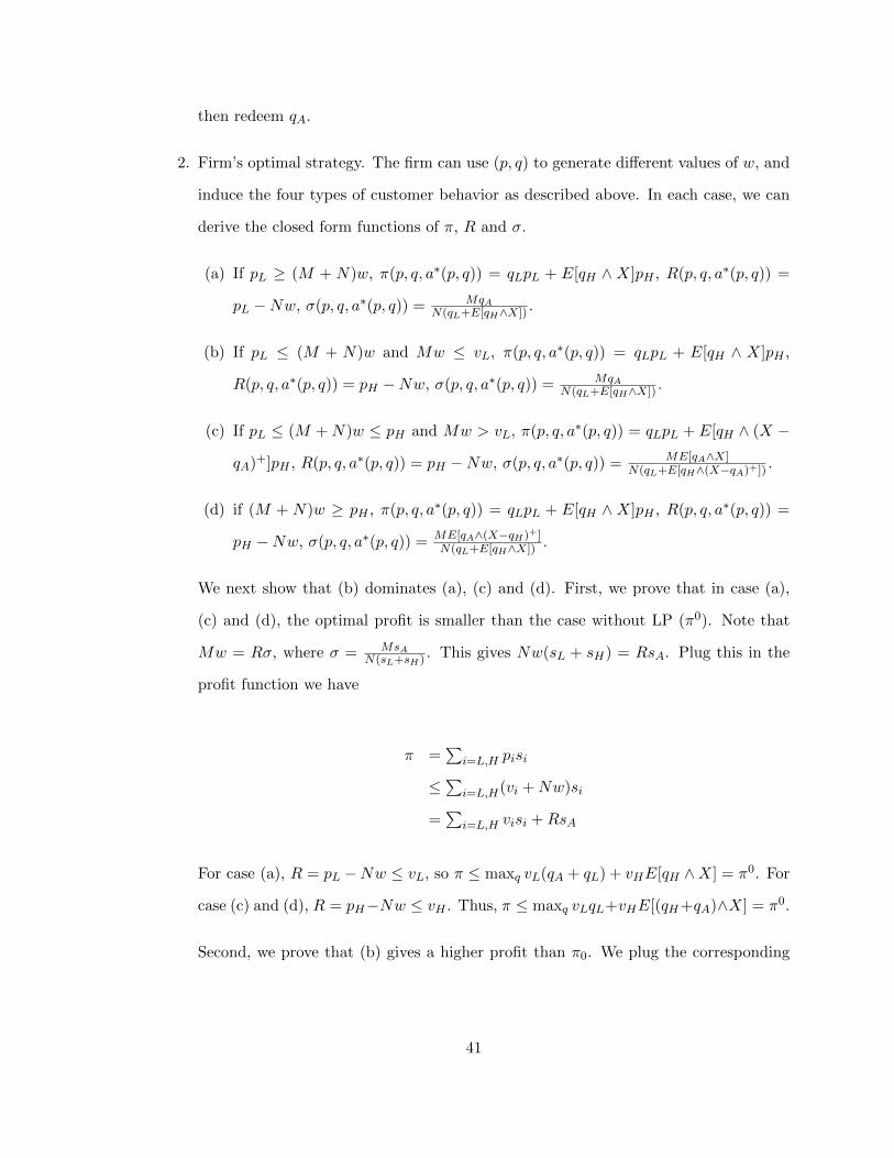
then redeem qA.

2. Firm’s optimal strategy. The firm can use (p, q) to generate different values of w, and

induce the four types of customer behavior as described above. In each case, we can

derive the closed form functions of π, R and σ.

(a) If pL ≥ (M + N)w, π(p, q, a∗(p, q)) = qLpL + E[qH ∧ X]pH , R(p, q, a∗(p, q)) =

pL −Nw, σ(p, q, a∗(p, q)) = MqAN(qL+E[qH∧X]) .

(b) If pL ≤ (M + N)w and Mw ≤ vL, π(p, q, a∗(p, q)) = qLpL + E[qH ∧ X]pH ,

R(p, q, a∗(p, q)) = pH −Nw, σ(p, q, a∗(p, q)) = MqAN(qL+E[qH∧X]) .

(c) If pL ≤ (M +N)w ≤ pH and Mw > vL, π(p, q, a∗(p, q)) = qLpL + E[qH ∧ (X −

qA)+]pH , R(p, q, a∗(p, q)) = pH −Nw, σ(p, q, a∗(p, q)) = ME[qA∧X]N(qL+E[qH∧(X−qA)+])

.

(d) if (M + N)w ≥ pH , π(p, q, a∗(p, q)) = qLpL + E[qH ∧ X]pH , R(p, q, a∗(p, q)) =

pH −Nw, σ(p, q, a∗(p, q)) = ME[qA∧(X−qH)+]N(qL+E[qH∧X]) .

We next show that (b) dominates (a), (c) and (d). First, we prove that in case (a),

(c) and (d), the optimal profit is smaller than the case without LP (π0). Note that

Mw = Rσ, where σ = MsAN(sL+sH) . This gives Nw(sL + sH) = RsA. Plug this in the

profit function we have

π =∑

i=L,H pisi

≤∑

i=L,H(vi +Nw)si

=∑

i=L,H visi +RsA

For case (a), R = pL −Nw ≤ vL, so π ≤ maxq vL(qA + qL) + vHE[qH ∧X] = π0. For

case (c) and (d), R = pH−Nw ≤ vH . Thus, π ≤ maxq vLqL+vHE[(qH+qA)∧X] = π0.

Second, we prove that (b) gives a higher profit than π0. We plug the corresponding

41

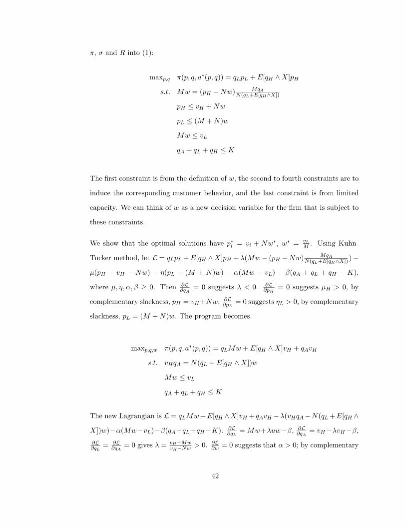
π, σ and R into (1):

maxp,q π(p, q, a∗(p, q)) = qLpL + E[qH ∧X]pH

s.t. Mw = (pH −Nw) MqAN(qL+E[qH∧X])

pH ≤ vH +Nw

pL ≤ (M +N)w

Mw ≤ vL

qA + qL + qH ≤ K

The first constraint is from the definition of w, the second to fourth constraints are to

induce the corresponding customer behavior, and the last constraint is from limited

capacity. We can think of w as a new decision variable for the firm that is subject to

these constraints.

We show that the optimal solutions have p∗i = vi + Nw∗, w∗ = vLM . Using Kuhn-

Tucker method, let L = qLpL +E[qH ∧X]pH + λ(Mw− (pH −Nw) MqAN(qL+E[qH∧X]))−

µ(pH − vH − Nw) − η(pL − (M + N)w) − α(Mw − vL) − β(qA + qL + qH − K),

where µ, η, α, β ≥ 0. Then ∂L∂qA

= 0 suggests λ < 0. ∂L∂pH

= 0 suggests µH > 0, by

complementary slackness, pH = vH+Nw; ∂L∂pL

= 0 suggests ηL > 0, by complementary

slackness, pL = (M +N)w. The program becomes

maxp,q,w π(p, q, a∗(p, q)) = qLMw + E[qH ∧X]vH + qAvH

s.t. vHqA = N(qL + E[qH ∧X])w

Mw ≤ vL

qA + qL + qH ≤ K

The new Lagrangian is L = qLMw+E[qH ∧X]vH + qAvH −λ(vHqA−N(qL +E[qH ∧

X])w)−α(Mw−vL)−β(qA+qL+qH−K). ∂L∂qL

= Mw+λuw−β, ∂L∂qA

= vH−λvH−β,

∂L∂qL

= ∂L∂qA

= 0 gives λ = vH−MwvH−Nw > 0. ∂L

∂w = 0 suggests that α > 0; by complementary

42

slackness, we have w∗ = vLM .

Therefore, p∗i = vi +Nw∗, w∗ = vLM , the problem becomes:

maxq vLqL + vH(qA + E[qH ∧X])

s.t. MvHqA = vLN(qL + E[qH ∧X])

qA + qL + qH ≤ K

(1.1)

Note that if the firm chooses q′L = q0, q′A and q′H such thatMq′A

N(q0+E[q′H∧X])= vL

vH, all

conditions are satisfied, which yields a profit of π′ = q0vL + q′AvH + E[q′H ∧ X] ≥

q0vL + E[qH ∧X] = π0. Thus the optimal solution in (b) must gives a profit higher

than π∗.

Rewrite (1) in terms of p∗ and σ∗:

maxq qLpL + E[qH ∧X]pH

s.t. MqA = σ∗N(qL + E[qH ∧X])

qA + qL + qH ≤ K

The new Lagrangian is L = qLpL +E[qH ∧X]pH +λ(MqA−σ∗N(qL +E[qH ∧X]))−

β(qA + qL + qH −K), where β ≥ 0. Take derivatives with respect to q:

∂L∂qA

= Mλ− β∂L∂qL

= pL − λσ∗N − β∂L∂qH

= F (qH)(pH − λσ∗N)− β

If ∂L∂qA

= ∂L∂qL

= ∂L∂qH

= 0, then λ = pLM+σ∗N , β = MpL

M+σ∗N , qH = q = F−1(MpL

M+σ∗N

pH−σ∗NpLM+σ∗N

).

Plugging these back in the condition qA + qL + qH = K and MqA = σ∗N(qL +E[qH ∧

X]), we get q∗L = MM+σ∗N (K − q − σ∗N

M E[q ∧ X]), q∗A = σ∗NM+σ∗N (K − q + E[q ∧ X]).

However, if K − q − σ∗NM E[q ∧ X] < 0, qL is negative. Thus the condition ∂L

∂qL= 0

43

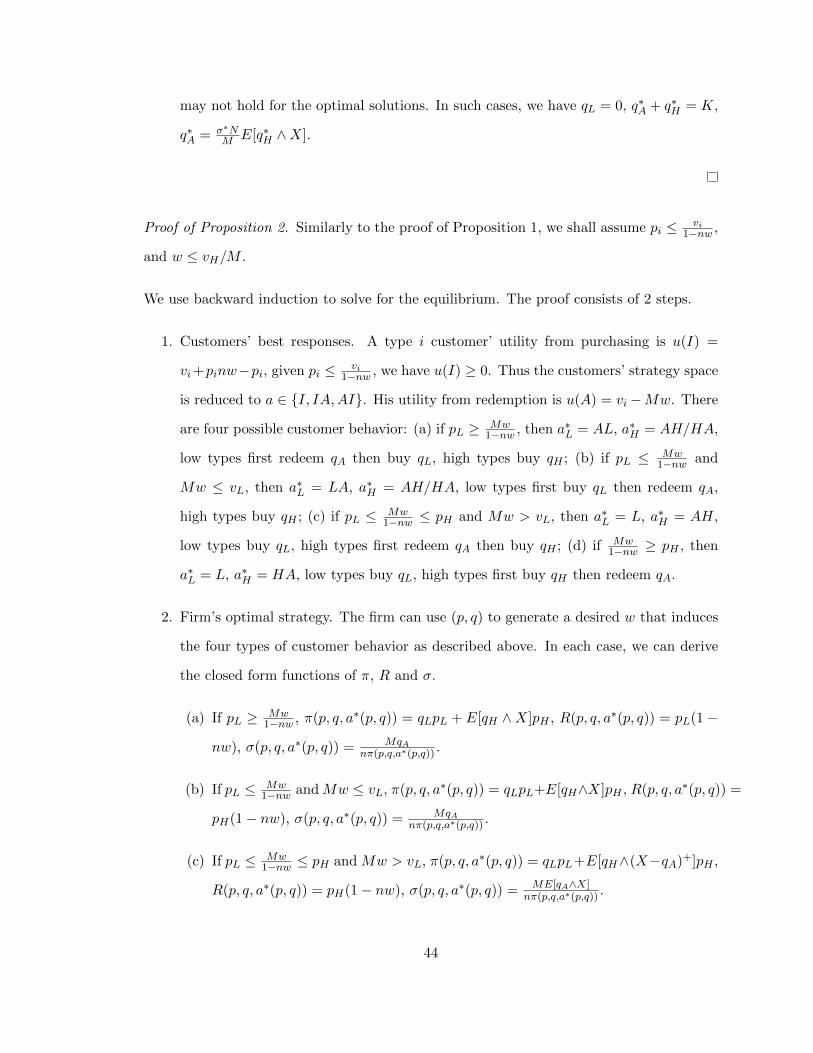
may not hold for the optimal solutions. In such cases, we have qL = 0, q∗A + q∗H = K,

q∗A = σ∗NM E[q∗H ∧X].

Proof of Proposition 2. Similarly to the proof of Proposition 1, we shall assume pi ≤ vi1−nw ,

and w ≤ vH/M .



vi+pinw−pi, given pi ≤ vi1−nw , we have u(I) ≥ 0. Thus the customers’ strategy space

is reduced to a ∈ {I, IA,AI}. His utility from redemption is u(A) = vi−Mw. There

are four possible customer behavior: (a) if pL ≥ Mw1−nw , then a∗L = AL, a∗H = AH/HA,

low types first redeem qA then buy qL, high types buy qH ; (b) if pL ≤ Mw1−nw and

Mw ≤ vL, then a∗L = LA, a∗H = AH/HA, low types first buy qL then redeem qA,

high types buy qH ; (c) if pL ≤ Mw1−nw ≤ pH and Mw > vL, then a∗L = L, a∗H = AH,

low types buy qL, high types first redeem qA then buy qH ; (d) if Mw1−nw ≥ pH , then

a∗L = L, a∗H = HA, low types buy qL, high types first buy qH then redeem qA.

2. Firm’s optimal strategy. The firm can use (p, q) to generate a desired w that induces

the four types of customer behavior as described above. In each case, we can derive

the closed form functions of π, R and σ.

(a) If pL ≥ Mw1−nw , π(p, q, a∗(p, q)) = qLpL + E[qH ∧X]pH , R(p, q, a∗(p, q)) = pL(1−

nw), σ(p, q, a∗(p, q)) = MqAnπ(p,q,a∗(p,q)) .

(b) If pL ≤ Mw1−nw andMw ≤ vL, π(p, q, a∗(p, q)) = qLpL+E[qH∧X]pH , R(p, q, a∗(p, q)) =

pH(1− nw), σ(p, q, a∗(p, q)) = MqAnπ(p,q,a∗(p,q)) .

(c) If pL ≤ Mw1−nw ≤ pH and Mw > vL, π(p, q, a∗(p, q)) = qLpL+E[qH∧(X−qA)+]pH ,

R(p, q, a∗(p, q)) = pH(1− nw), σ(p, q, a∗(p, q)) = ME[qA∧X]nπ(p,q,a∗(p,q)) .

44

(d) if Mw1−nw ≥ pH , π(p, q, a∗(p, q)) = qLpL +E[qH ∧X]pH , R(p, q, a∗(p, q)) = pH(1−

nw), σ(p, q, a∗(p, q)) = ME[qA∧(X−qH)+]nπ(p,q,a∗(p,q)) .

We next show that (b) dominates (a), (c) and (d). First, we prove that in case (a),

(c) and (d), the optimal profit is smaller than the case without LP (π0). Note that

Mw = Rσ, where σ = MsAnπ . This gives nwπ = RsA. Plug this in the profit function

we have

π =∑

i=L,H pisi

≤∑

i=L,Hvi

1−nwsi

=∑

i=L,H visi + nwpisi

=∑

i=L,H visi + nwπ

=∑

i=L,H visi +RsA

For case (a), R = pL(1−nw) ≤ vL, so π ≤ maxqA,qL,qH vL(qA+qL)+vHE[qH∧X] = π0.

For case (c) and (d), R = pH(1−nw) ≤ vH . Thus, π ≤ maxqA,qL,qH vLqL+vHE[(qH +

qA) ∧X] = π0.

Second, we prove that (b) gives a higher profit than π0. We plug the corresponding

a∗, π, σ and R into (1):

maxp,q π(p, q, a∗(p, q)) = qLpL + E[qH ∧X]pH

s.t. Mw = pH(1− nw) MqAn(qLpL+E[qH∧X]pH)

pi ≤ vi1−nw

pL ≤ Mw1−nw

Mw ≤ vL

qA + qL + qH ≤ K

Similarly, we can think of w as a new decision variable that is subject to those con-

straints. We shall show that the optimal solutions have p∗i = vi1−nw∗ , w

∗ = vLM .

45

Using Kuhn-Tucker method similar to the proof of Proposition 1, we have w∗ = vLM ,

p∗i = vi1−nw∗ .

Therefore, the problem becomes:

maxq vLqL + vH(qA + E[qH ∧X])

s.t. MvHqA = vLn(vLqL + vH(qA + E[qH ∧X]))

qA + qL + qH ≤ K

(1.2)

Note that if the firm chooses q′L = q0, q′A and q′H such thatMq′A

n(vLqL+vH(qA+E[qH∧X])) =

vLvH

, all conditions are satisfied, which yields a profit of π′ = q0vL+q′AvH+E[q′H∧X] ≥

q0vL + E[qH ∧X] = π0. Thus the optimal solution in (b) must gives a profit higher

than π∗.

Rewrite (2) in terms of p∗ and σ∗:

maxpH ,qj qLpL + E[qH ∧X]pH

s.t. MqA = σ∗n(qLpL + E[qH ∧X]pH)

qA + qL + qH ≤ K

The new Lagrangian function is L = qLpL + E[qH ∧ X]pH + λ(MqA − σ∗n(qLpL +

E[qH ∧X]pH))− β(qA + qL + qH −K), where β ≥ 0. Take derivatives with respect to

q we have

∂L∂qA

= λM − β∂L∂qL

= pL(1− λσ∗n)− β∂L∂qH

= F (qH)pH(1− λσ∗n)− β

If ∂L∂qA

= ∂L∂qL

= ∂L∂qH

= 0, then λ = σ∗npLM+σ∗npL

, β = Mσ∗npLM+σ∗npL

, qH = q = F−1( vLvH ).

Plugging these back in the constraints qA + qL + qH = K and MqA = σ∗n(qLpL +

46

E[qH ∧X]pH), we get q∗L = MM+σ∗np∗L

(K− q− σ∗np∗HM E[q∧X]), q∗A = σ∗n

M+σ∗np∗L(p∗L(K−

q) + p∗HE[q ∧ X]). However, if K − q − σ∗np∗HM E[q ∧ X] < 0, qL is negative. In such

cases, we have q∗L = 0, q∗A and q∗H satisfies q∗A + q∗H = K, q∗A =σ∗np∗HM E[q∗H ∧X].

Proof of Proposition 3. Similarly to the proofs of Proposition 1 and 2, we shall assume

pi ≤ vi1−nw , and w ≤ 1

m+n .



vi + pinw − pi, given pi ≤ vi1−nw , we have u(I) ≥ 0. Thus the customers’ strategy

space is reduced to a ∈ {I, IA,AI}. His utility from redemption is u(A) = vi−mpiw.

Since (m + n)w ≤ 1, we have two possible customer behavior: (a) if (m + n)w ≤ 1,

then u(A) ≥ u(I) for I = L,H, a∗L = AL, a∗H = AH, low types first redeem qA then

buy qL, high types buy qH . (b) if (m + n)w = 1, then u(I) < u(A) for I = L,H

and pi = pL, pH , a∗L = L, a∗H = HA, low types first buy qL, high types buy qH then

redeem qA; (b)

2. Firm’s optimal strategy. Rewrite the firm’s profit as

π =∑

i=L,H pisi

≤∑

i=L,Hvi

1−nwsi

=∑

i=L,H visi + nwpisi

=∑

i=L,H visi + nwπ

=∑

i=L,H visi +RsA

The firm can use (p, q) to generate a desired w that induces the two types of customer

behavior as described above. In each case, we can derive the closed form functions of

π, R and σ.

47

(a) If (m + n)w ≤ 1, a∗L = AL, a∗H = AH, π(p, q, a∗(p, q)) = qLpL + E[qH ∧X]pH .

There are two cases. If qL > 0, R(p, q, a∗(p, q)) = pL(1− nw), σ(p, q, a∗(p, q)) =

mpLqAnπ(p,q,a∗(p,q)) . We have

π ≤∑

i=L,H visi +RsA

=∑

i=L,H visi + pL(1− nw)sA

≤∑

i=L,H vL(qA + qL) + vHE[qH ∧X]

≤ π0

The Littlewood profit is attainable at pi = vi1−nw , qH = q0

H , qA + qL = q0L and

q∗A ∈ [0, nm(qL + vHvLE[q0

H ∧X])] (so the redemption rate σ ≤ 1).

If qL = 0, R(p, q, a∗(p, q)) = pH(1 − nw), σ(p, q, a∗(p, q)) = mpHqAnπ(p,q,a∗(p,q)) . The

optimal profit in this case is

maxp,q π(p, q, a∗(p, q)) = E[qH ∧X]pH

s.t. Mw = pH(1− nw) pHmqAnE[qH∧X]pH

pH ≤ vH1−nw

(m+ n)w ≤ 1

qA + qH ≤ K

By solving this program, we have pH = vH1−nw , qA = vLn

vHmE[qH∧X], w = vL

vLn+vHm.

The profit is πa = vH(qA + E[qH ∧X]).

(b) If (m + n)w = 1, a∗L = L, a∗H = HA, π(p, q, a∗(p, q)) = qLpL + E[qH ∧ X]pH ,

48

R(p, q, a∗(p, q)) = pH(1− nw), σ(p, q, a∗(p, q)) = mpHE[(X−qH)+∧qA]nπ(p,q,a∗(p,q)) . We have

π ≤∑

i=L,H visi +RsA

=∑

i=L,H visi + pH(1− nw)sA

≤∑

i=L,H vLqL + vHE[(qH + qA) ∧X]

≤ π0

The Littlewood profit is attainable at pi = vi1−nw , qL = q0

L, qA + qH = q0H and

E[(X − qH)+ ∧ qA] ∈ [0, nm( vLvH q0L + E[qH ∧X])] (so the redemption rate σ ≤ 1).

As a final step, we need to compare πa from closing the low price capacity and and

π0 from the Littlewood benchmark. Note that when K is small, q0L = 0, π0 =

vHE[K ∧X] ≤ vH((K− qH) +E[qH ∧X]) = πa. It suffices to show that when q0L > 0,

there exists K, such that πa ≥ π0 iff K ≤ K. Note that when q0L ≥ 0, ∂π0

∂K = vL,

∂2π0

∂K2 = 0. In contrast, ∂πa

∂K = vH1+

nvLmvH

1F (qH )

+nvLmvH

, ∂2πa

∂K2 = ∂πa

∂F (qH)∂F (qH)∂qH

∂qH∂K ≤ 0. Therefore,

∂2π0−πa∂K2 < 0, and π0−πa when qL = 0, so there exists K such that πa ≥ π0 iff K ≤ K.

∂πa

∂K = vH ,

49

CHAPTER 2 : LOYALTY PROGRAMS AND CONSUMER CHOICE:

EVIDENCE FROM AIRLINE INDUSTRY

We study customers’ valuation of loyalty program points. By using airlines survey data,

we compute customers’ willingness to pay (WTP) for points at issuance and willingness

to accept (WTA) at redemption. We demonstrate that compared to the objective value

of miles, customers over-evaluate miles both at issuance (by 139%) and redemption (by

346%). The huge difference may result from overconfidence of the redemption value and

redemption probability. We also show that airlines can improve profits (up to 7%) by simply

manipulating program designs.

2.1. Introduction

Loyalty programs have been ubiquitous in modern industries. A frequent-flyer program

(FFP) is a loyalty program offered by an airline. Such programs are designed to encourage

airline customers to accumulate “miles” which may then be redeemed for air travel or other

rewards.

The miles earned and redeemed under FFPs may be price-dependent or independent. The

most traditional program type is mileage-based programs, in which both the issuance and

redemption are price-independent: while the number of the issued miles equal to the flying

distance of the customer, the number of redeemed miles is fixed for domestic flight. For

example, consider a customer who flies from Philadelphia to San Francisco. Under a mileage-

based program, he earns 2,515 miles (the distance) no matter how much he pays; when he

wishes to redeem a domestic flight, he spends 25,000 miles. Contrary to mileage-based

programs, fare-based programs determine both the number of issued miles and the number

of redeemed miles proportional to the price the customer pays. In the previous example,

suppose the airline changes to a fare-based program which issues 5 miles for every dollar

the customer pays and requires 60 miles for every dollar he redeem. If the price is $500,

then the customer earns 25,00 miles for a cash-paid ticket, and redeems 300,000 miles for

50

an award ticket; if the price is $300, then the numbers reduce to 1,500 miles and 180,000

miles respectively. Finally, a third type of program is mixed-program, in which the issuance

is proportional to the price (like in a fare-based program) and the redemption is fixed (like

in a mileage-based program).

Ever since American Airlines launched its AAdvantage mileage program in 1981, almost

every airlines started with a mileage-based program. However, the industry has witnessed

a recent trend of changing toward price-dependent issuance and redemption. For example,

JetBlue (True Blue) and Southwest Airlines (Rapid Rewards) changed to fare-based pro-

grams around 2010. United Airlines and Delta Airlines offered their new mixed programs

in 2014; American Airlines followed in 2016.

These program changes imposed an impact on the value of frequent flyer miles, which have

emerged as a virtual currency. Typically, customers earn miles for their purchases and sub-

sequently redeem them for rewards. It has been shown that frequent flyer program members

are willing to spend 2% to 12% more for similar itineraries provided by the program carrier

than by other airlines (Brunger, 2013). In fact, casual assessments tend to put the value of

most loyalty points at between $0.01 and $0.02 each; for example, an AAdvantage mile is

estimated to be worth $0.017 (BoardingArea, 2014). Despite the heating discussions about

the value of frequent flyer miles in different programs, it remains unclear how customers

evaluate miles at their purchasing and redemption decisions.

Our research aims to investigate how customers evaluate this virtual currency given different

program designs and rewarding rules. Specifically, we look at three levels of the values:

Market value of miles Since miles can be used to redeem for flight ticket, their market

value can be calculated based on the market price of the awarded ticket. For instance,

suppose for airline i, the every price of a ticket redeemed by 25,000 miles is $500, then the

market value of a mile is $0.02. This reflects the objective value of miles (OBJ).

51

Value of miles at issuance When customers accumulate miles by paying cash, they

may be willing to pay additionally for more issued miles. We are interested in the amount

of cash price the customers are willing to pay for the issued miles. This reflects customers’

subjective willingness to pay (WTP) as buyers of miles.

Value of miles at redemption When customers spend miles to redeem award, they

compare the mile price to the cash price. We are interested in the customers’ disutility of

spending miles as opposed to spending cash. This reflects customers’ subjective willingness

to accept (WTA) as sellers of miles.

The goal is to calculate each level of the values, and study how they influence customers’

choice decisions at both the purchasing point and redemption point. While many frequent

flyers calculated that each mile is worth 1-2 cents based on the value of a redeemable

award, the question remains unclear whether customers make decisions according to this

value. We shall calibrate both the objective and the subjective values of miles from real

customer transaction data. Moreover, we will address the following questions.

• How do the WTP and WTA of miles compare to the objective market values (OBJ)?

• Do operational decisions (award availability, award choices and award rules) impact

how customers evaluate miles and consequently their decision-making processes?

• Do miles carry different values in different airlines and at different locations? What

is the impact of program changes on the values?

Finally, given the value of miles, we are also interested in its interpretations on the airlines’

profits. Specifically, the number of issued miles varies across program designs and may

result in different impacts on revenues. Which program design is most profitable? Do

airlines benefit from changing to fare-based issuance of frequent flyer miles? We shall

address these questions in the study.

Our work is related to the literature on consumer behavior in the context of loyalty pro-

52

grams. Many papers have studied how consumers perceive and value loyalty points as an

independent currency. Using a reference dependence framework, Dreze and Nunes (2004)

developed a mental accounting model where customers evaluate different currencies (i.e.,

cash and loyalty points) in separate accounts; Stourm et al. (2015) recently extended

this mental accounting model to explain why many customers stockpile loyalty points even

though the firm does not reward such behavior. In another study, van Osselaer et al. (2004)

showed that loyalty points are an overvalued currency and create an illusion of progress.

In a similar vein, Kivetz et al. (2006) and Nunes and Dreze (2006) showed that artificial

advancement (e.g., replacing a 10-stamp coffee card with a 12-stamp card that starts with

2 stamps already filled in) increases customer effort; the former study also found evidence

of purchase acceleration as customers come closer to earning rewards. These results suggest

that customers place an explicit value on each loyalty point even though loyalty points are

only a medium (i.e., a means to an end); see Hsee et al. (2003) on the medium effect. Fi-

nally, Raghubir and Srivastava (2002) and Wertenbroch et al. (2007) found that consumers’

valuation of an unfamiliar currency (such as loyalty points) is biased towards the face value;

a possible explanation is that consumers anchor on the nominal face value and do not adjust

sufficiently for the exchange rate when making decisions. Sayman and Hoch (2014) showed

that buyers are willing to pay a price premium for loyalty points, and the premium is less

than the normative levels. Motivated by these behavioral studies, our theoretical model

takes the view that each loyalty point is a unit of currency valued at the nominal face value

of goods that it can be redeemed for.

2.2. Data

The primary database we used is Airline Origin and Destination Survey (DB1B) conducted

by Bureau of Transportation Statistics. It is a 10% sample of airline tickets from report-

ing carriers. Data includes origin, destination and other itinerary details of passengers

transported.

To compare the effect of program change in early 2015, we used data in 2014 and 2015. Each

53

quarter has more than 1 million itineraries over around 10 thousand routes operated by 27

carriers. We restricted our analysis to round-trip itineraries with an origin at large/medium

hubs (with a ranking smaller or equal to 61 in Passenger Boarding (Enplanement) and All-

Cargo Data for U.S. Airports). This accounts for 87.7% of total data.

Table 4-4 summarize the statistics of major airlines in the dataset in both years. Between

the year of 2014 and 2015, the industry witnessed an overall price drop and demand in-

crease, with two exceptions. United Airlines increased its price at the cost of demand loss.

Southwest decreased its price but still had demand loss. Note that these numbers were

calculated by aggregating all itineraries and routes.

Besides DB1B database, two other databases were used. First, the census population data

for the origin cities was utilized to calculate the total market base. Second, the airline on-

time performance data was used to get information about the take-off time of each flight,

as well as the delay frequency and duration.

54

Table 3: Summary Statistics (2014)

Airlines American Alaska United Delta Southwest JetBlue Frontier

Routes 2607 169 1081 2267 4082 240 426Total Passengers 1663509 315565 1025765 1488061 3061011 515823 260145

Average Passengers 164.5 539.4 246.3 177.5 173.8 538.7 199.0lightgrayAverage Price 225.0 178.8 252.4 238.6 179.3 192.0 137.1

yellow Average Distance 1156.8 1112.6 1363.8 1106.5 880.6 1241.0 1014.5greenAverage Miles Awarded 1156.8 1112.6 1363.8 1106.5 1075.8 1152.0 1014.5

Origin Flight Share 14.8% 15.8% 17.8% 17.3% 40.2% 19.5% 3.5%Award Fraction 6.3% 5.7% 9.2% 8.7% 11.5% 3.9% 2.9%

Table 4: Summary of Statistics (2015)

Airlines American Alaska United Delta Southwest JetBlue Frontier

Routes 2636 140 1214 2230 4763 267 401Total Passengers 1673525 349751 1071056 1529566 2675637 553929 338724

Average Passengers 175.1 672.6 245.3 180.1 170.1 553.6 281.1lightgrayAverage Price 209.2 180.5 241.9 232.7 175.8 190.1 106.6yellowAverage Distance 1163.1 1120.7 1349.6 1108.0 908.3 1249.9 1072.5

greenAverage Miles Awarded 1163.1 1120.7 1209.5 1163.5 1054.8 1140.6 1072.5Origin Flight Share 14.1% 15.4% 33.8% 21.8% 30.3% 19.4% 2.7%

Award Fraction 5.4% 5.4% 8.9% 8.2% 12.0% 6.9% 1.5%

55

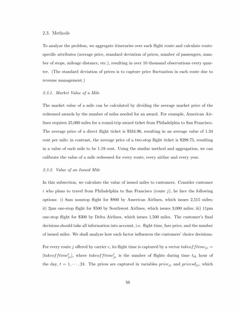
2.3. Methods

To analyze the problem, we aggregate itineraries over each flight route and calculate route-

specific attributes (average price, standard deviation of prices, number of passengers, num-

ber of stops, mileage distance, etc.), resulting in over 10 thousand observations every quar-

ter. (The standard deviation of prices is to capture price fluctuation in each route due to

revenue management.)

2.3.1. Market Value of a Mile

The market value of a mile can be calculated by dividing the average market price of the

redeemed awards by the number of miles needed for an award. For example, American Air-

lines requires 25,000 miles for a round-trip award ticket from Philadelphia to San Francisco.

The average price of a direct flight ticket is $334.96, resulting in an average value of 1.34

cent per mile; in contrast, the average price of a two-stop flight ticket is $298.75, resulting

in a value of each mile to be 1.19 cent. Using the similar method and aggregation, we can

calibrate the value of a mile redeemed for every route, every airline and every year.

2.3.2. Value of an Issued Mile

In this subsection, we calculate the value of issued miles to customers. Consider customer

i who plans to travel from Philadelphia to San Francisco (route j), he face the following

options: i) 8am nonstop flight for $800 by American Airlines, which issues 2,515 miles;

ii) 2pm one-stop flight for $500 by Southwest Airlines, which issues 3,000 miles; iii) 11pm

one-stop flight for $300 by Delta Airlines, which issues 1,500 miles. The customer’s final

decisions should take all information into account, i.e. flight time, fare price, and the number

of issued miles. We shall analyze how each factor influences the customers’ choice decisions.

For every route j offered by carrier c, its flight time is captured by a vector takeofftimejc =

[takeofftimetjc], where takeofftimetjc is the number of flights during time tth hour of

the day, t = 1, · · · , 24. The prices are captured in variables pricejc and pricesdjc, which

56

measure the mean and stand deviation of prices respectively. The number of issued miles

is captured by milesearnedjc. Here, for mileage-based programs, we have milesearnedjc =

distancej , where distancej is the flying distance of route j; for fare-based programs, we

have milesearnedjc = issueratec · pricejc, where issueratec = 6 for Southwest Airlines,

issueratec = 5 for United Airlines and Delta Airlines. (We didn’t consider JetBlue here

because the issuing policy varies by purchasing channels.)

Note that the effect of the issuing miles may be dependent on the future values of the miles,

which further relies on their easiness of redemption. Without loss of generosity, we use

two factors to capture the easiness of redemption: redemption rate and redemption choices.

Hence, we shall include the interaction of these factors into the regression function as well.

The award redemption rate can be estimated using origin-carrier (OC) pairs. Specifically, we

use fracawardoc as a proxy for reward redemption rate, where fracawardoc is the fraction

of reward passengers over all passengers for all the routes from an origin o by carrier c.

For example, at Philadelphia International Airport, American Airlines rewards 5.96% of its

tickets, so we have fracawardoc = 0.0596. Note that this metric is the joint result of both

award supply and award demand. Nevertheless, for most Airlines except Southwest, the

award availability is below 90% (IdeaWorks Survy); hence, fracawardoc is more of a valid

metric for award supply than demand. Even in the case of Southwest, when fracawardoc

purely reflects award demand, it should still be positively correlated with award redemption

rate.

Similarly, we use OC pairs to calibrate redemption choices. One hypothesis is the following:

if a higher fraction of future flights at the customers’ home airport o is carried by airline

c, the customer has more opportunities to use the miles issued by c. Hence, the expected

future value of miles becomes higher, and the customer is more likely to be influenced by the

issuance of miles. To capture this effect, we use flightshareoc as a proxy for the proportion

of future flights carried by c, where flightshareoc equals to the fraction of flight routes

offered by c over all the flight routes from origin o.

57

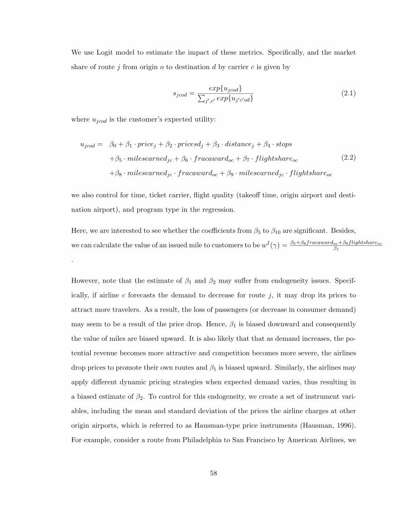
We use Logit model to estimate the impact of these metrics. Specifically, and the market

share of route j from origin o to destination d by carrier c is given by

sjcod =exp{ujcod}∑

j′,c′ exp{uj′c′od}(2.1)

where ujcod is the customer’s expected utility:

ujcod = β0 + β1 · pricej + β2 · pricesdj + β3 · distancej + β4 · stops

+β5 ·milesearnedjc + β6 · fracawardoc + β7 · flightshareoc

+β8 ·milesearnedjc · fracawardoc + β9 ·milesearnedjc · flightshareoc

(2.2)

we also control for time, ticket carrier, flight quality (takeoff time, origin airport and desti-

nation airport), and program type in the regression.

Here, we are interested to see whether the coefficients from β5 to β10 are significant. Besides,

we can calculate the value of an issued mile to customers to be wI(γ) = β5+β8fracawardoc+β9flightshareocβ1

.

However, note that the estimate of β1 and β2 may suffer from endogeneity issues. Specif-

ically, if airline c forecasts the demand to decrease for route j, it may drop its prices to

attract more travelers. As a result, the loss of passengers (or decrease in consumer demand)

may seem to be a result of the price drop. Hence, β1 is biased downward and consequently

the value of miles are biased upward. It is also likely that that as demand increases, the po-

tential revenue becomes more attractive and competition becomes more severe, the airlines

drop prices to promote their own routes and β1 is biased upward. Similarly, the airlines may

apply different dynamic pricing strategies when expected demand varies, thus resulting in

a biased estimate of β2. To control for this endogeneity, we create a set of instrument vari-

ables, including the mean and standard deviation of the prices the airline charges at other

origin airports, which is referred to as Hausman-type price instruments (Hausman, 1996).

For example, consider a route from Philadelphia to San Francisco by American Airlines, we

58

use the pricing information of all AA flights going to San Francisco from places other than

Philadelphia as instruments. It captures the characteristics of the airlines’ general pricing

schemes, but does not include any other information from the route “market” (since the

“market” is based on the origin - Philadelphia). We run a two step least squares regressions.

2.3.3. Value of a Redeemed Mile

In this subsection, we calculate the value of a redeemed mile. Consider a customer who has

accumulated enough miles to redeem for a free flight ticket with carrier c. At each travel

opportunity, he chooses between redeeming his miles and paying cash to save the miles for

future use. For example, suppose he flies from Philadelphia and San Francisco. The current

cash price is $500, while the required miles for a redemption is 25,000. He compares the

two options.

Using Logit model, the fraction of customers who pay cash for route j is given by

cj =exp{ucj}

exp{ucj}+ exp{umj }(2.3)

the rest is the proportion of customers who pay miles:

mj =exp{umj }

exp{ucj}+ exp{umj }(2.4)

Here, ucj and umj are the customers’ expected utility from using cash ($500) and miles (25,000

miles) for route j, respectively. Apparently, if the price in cash is high, the customers’

utility from paying cash (ucj) is lower, if the price in miles or the value of miles is high,

then the customers’ utility from using the miles (umj ) is low. The value of miles depends

on the chances of a future redemption using those miles, which might be dependent of the

redemption rate (fracredeemedoc) and redemption choices (flightshareoc).

59

Thus, we can model these effects in a simple regression

logmj

1−mj = umj − ucj = γ0 + γ1 · pricej + γ2 · pricesdj + γ3 · distancej + γ4 · stops

+γ5 ·milesredeemedjc + γ6 · fracawardoc + γ7 · flightshareoc

+γ8 ·milesredeemedjc · fracawardoc + γ9 ·milesredeemedjc · flightshareoc(2.5)

We are interested to estimate γ1, γ5, γ8 and γ9 and test whether they are significantly

different from 0. Intuitively, γ1 ≥ 0 (higher cash prices, more redemption), γ5 ≤ 0 (higher

mile prices, fewer redemption), γ8 ≤ 0 and γ9 ≤ 0 (easier redemptions, higher value of

miles). Moreover, the value of one mile should be equal to |γ7+γ8·fracawardoc+γ9·flightshareoc|γ1

.

However, note that the effect of fracawardoc does not only impact the customers’ future

redemptions, but also reflect the convenience of the current redemption as well. Specifically,

if fracawardoc is high, the award capacity of the route is likely to be higher and the customer

find it easier to redeem his miles. This results in a higher mj and a positive γ8, which biases

the value of miles downward. Hence, the effect of future award availability on the value

of miles cannot be accurately predicted by fracaward, so we exclude it from regression.

Besides, the value of a redeemed mile may also be route-dependent, i.e., for those routes

with higher values, the redeemed miles carry higher values. To capture this effect, we use a

variable destpriced, which equals to the average price of all routes to the same destination

from other origins. This variables is a proxy for the value of the route, without using any

market price information of the origin airport. Hence, the regression equation is updated

below.

logmj

1−mj = umj − ucj = γ0 + γ1 · pricej + γ2 · pricesdj + γ3 · distancej + γ4 · stops

+γ5 ·milesredeemedjc + γ6 · destpriced + γ7 · flightshareoc

+γ8 ·milesredeemedjc · destpriced+

γ9 ·milesredeemedjc · flightshareoc + γ10 ·milesredeemedjc · fracawardoc(2.6)

60

Similarly, the estimate of γ1 may suffer from endogeneity issues. Specifically, if the route is

more “touristic” (i.e., it has more leisure customers who wish to redeem miles), the firm may

adjust prices as follows. First, the firm anticipates more redemptions, hence fewer capacity

sold for cash. It increases cash prices to sell to a smaller group of high-end cash-paying

customers. This inflates the estimate γ1. Second, the firm anticipates higher demand for

redemptions. To maintain the volume of cash sales, it decreases cash prices to induce more

cash purchases. This deflates the estimate of γ1.

Both endogeneity problems come from the unobserved demand for the route. We control

this by including origin and destination in the regression equation. Besides, we also use the

same set of instrument variables for the mean and standard deviation of prices.

Finally, note that we model the issuance and redemption separately. In the previous sec-

tion, customers can purchase with cash from all airlines, but can not redeem miles. The

simplification can be justified by two assumptions: (i) the customers are business travelers

who only spend cash for the trip; (ii) the customers haven’t accumulated enough miles for

an award redemption. In contrast, this section allows customers to redeem miles, but does

not consider the customers’ outside option of using cash for other airlines. This assumption

can be justified by the following reasons. First, since the customer has accumulated enough

miles for a redemption, he must be a “frequent flyer” with carrier c. It is very likely that

c is his preferred carrier. Research has shown that customers are willing to pay up to 12%

more for similar itineraries provided by their major program carrier than by other airlines

(Brunger, 2013). The customer may prefer to spending more with carrier c rather than

switching to other carriers. Second, for all the origin airports we have, the dominant carri-

ers offer around 49.29% of all flights, while the second popular carrier only carries 17.15% of

all flights. Hence, competition is not very intense and we can assume that customers stick

with one carrier once they accumulate enough miles. By these assumptions, we restrict the

customers’ choices to the simple binary decisions.

61

2.4. Results: Value of Miles

2.4.1. Market Value of Miles (Objective Value)

The average price of a redeemed ticket is $207.52, resulting in a value of one mile around

0.83 cent. This value is well below the 1.4 cent per mile benchmark calculated by Tripadvi-

sor.com. Decomposing the redemptions into each airlines and both years yields the following

table. (The values of Southwest and JetBlue miles are calculated by using program rules. )

Table 5: Market Value of a Mile (Unit: Cent)

Airlines American Alaska United Delta Southwest JetBlue

2014 0.98 0.77 1.07 1.04 1.67 1.40

2015 0.80 0.81 1.05 0.98 1.49 1.40

The most valuable miles are from Southwest Airlines. Their program allowed 60 miles to

account for one dollar at redemption, yielding one mile to be worth of 1.67 cent. In 2015,

Southwest devalued its miles by increasing the exchange rate to 70:1 from April. This

resulted in an average value of 1.49 cent per mile throughout the year. The least valuable

miles are from Alaska Airlines, due to low prices of the redeemed tickets ($192.14 in 2014

and $201.40 in 2015).

Moreover, we can also calculate the value of miles for every route. The most valuable

redemption is flying directly from New York (EWR) to Dallas (DFW) by American Airlines,

yielding a value of 2.25 cent per mile. The least valuable redemption is flying directly from

Las Vegas (LAX) to Salt Lake City (SLC), yielding a value of 0.64 cent per mile.

2.4.2. Value of an Issued Mile (WTP)

We first run model (2.1) - (2.2) and summarize the results in Table 6.

The key observations are as follows:

62

1. Higher prices lead to lower customer utility. More revenue management (higher stan-

dard deviation of prices) leads to a higher chance of finding a bargain and hence higher

customer utility.

2. Miles are worthless when award space and award choices are non-existent (fracaward

and flightshare are standardized). Miles become a scam and may generate negative

utility to customers. Only when there is any redemption options do customers value

miles.

3. The average value of an issued mile is 3.64 cent.

4. Award availability (fracaward) has a negative impact on customer utility (perhaps

due to the reduced availability for cash purchases), but a positive impact on the value

of frequent flyer miles (customers enjoy the easiness of redemption).

5. Award choices (flightshare) has a positive impact on customer utility (since cus-

tomers are likely to be members of dominant programs), but do not have any impact

on the value of frequent flyer miles.

63

Table 6: Consumer Choice Model (Issued Miles)

Dependent Variable: Consumer Utility

OLS Regression 2SLS Regression

Model 1 Model 2 Model 3 Model 4

price −0.0239∗∗∗−0.0265∗∗∗−0.0429∗∗∗−0.0197∗∗∗

(0.0009) (0.0011) (0.0043) (0.0040)

pricesd 0.0372∗∗∗ 0.0357∗∗∗ 0.0632∗∗∗ 0.0722∗∗∗

(0.0013) (0.0013) (0.0060) (0.0059)

stops −21.3500∗∗∗−21.0000∗∗∗−21.1100∗∗∗−20.5200∗∗∗

(0.1254) (0.1285) (0.1627) (0.1637)

distance −0.0023∗∗∗−0.0027∗∗∗−0.0018∗∗∗−0.0040∗∗∗

(0.0001) (0.0001) (0.0002) (0.0002)

milesearned 0.0004∗∗∗ 0.0007∗∗∗

(0.0001) (0.0002)

fracaward −3.2750 −35.6800∗∗∗

(3.1800) (3.9670)

flightshare 12.2500∗∗∗ −0.2018

(0.6260) (2.2230)

milesearned · fracaward 0.0007 0.0215∗∗∗

(0.0039) (0.0055)

milesearned · flightshare −0.0003 −0.0004

(0.0005) (0.0007)

ticketcarrier X X X X

origin X X X X

destination X X X X

year X X X X

quarter X X X X

ontimes X X X X

takeofftime X X X X

farebased X X X X

R2 0.7370 0.7405 0.7355 0.7305

Adj. R2 0.7365 0.7400 0.7351 0.7300

6. The value of miles in cash can be predicted below with and without IV (we exclude

JetBlue because the issuance rules depend on the purchasing channel):

64

Figure 5: Value of Issued Miles

Table 7: Value of an Issued Mile without IV (Unit: Cent)

(Market Value in Parenthesis)

Airlines American Alaska United Delta Southwest

2014 1.68 (0.98) 1.65 (0.77) 1.72 (1.07) 1.72 (1.04) 1.51 (1.67)

2015 1.68 (0.80) 1.67 (0.81) 1.52 (1.05) 1.65 (0.98) 1.64 (1.49)

Table 8: Value of an Issued Mile with IV (Unit: Cent)



2014 1.95 (0.98) 0.47 (0.77) 3.76 (1.07) 3.69 (1.04) 5.94 (1.67)

2015 1.00 (0.80) 0.80 (0.81) 3.28 (1.05) 2.99 (0.98) 6.69 (1.49)

Key observations from Table 8:

(a) Southwest miles have the highest value (5.94-6.69cent), almost four times of the

1.4cent benchmark.

(b) Alaska miles have the lowest value (0.47 cent) in 2014, but its value improved in

65

2015 due to enhanced award capacity (a 6.4% improvement from 4.67% award

capacity in 2014 to to 4.97% award capacity in 2015).

(c) The most valuable miles are Southwest Airlines at ABQ (12.22 cent per mile),

followed by Delta Airline miles at CVG (8.27cent per mile). (CVG is a hub

airport of Delta Airlines).

(d) The least valuable miles are Alaska Airline miles at BDL, with 0% award capacity.

2.4.3. Value of a Redeemed Mile (WTA)

We first run the models and summarize the results in Table 9.

66

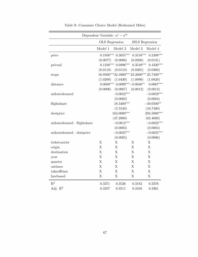
Table 9: Consumer Choice Model (Redeemed Miles)

Dependent Variable: uc − um

OLS Regression 2SLS Regression

Model 1 Model 2 Model 3 Model 4

price 0.1956∗∗∗ 0.3055∗∗∗ 0.3158∗∗∗ 0.2498∗∗∗

(0.0077) (0.0086) (0.0200) (0.0131)

pricesd 0.1238∗∗∗ 0.0896∗∗∗ 0.3549∗∗∗ 0.4330∗∗∗

(0.0110) (0.0110) (0.0265) (0.0260)

stops 16.9500∗∗∗22.4900∗∗∗ 23.3800∗∗∗ 25.7400∗∗∗

(1.0200) (1.0430) (1.0890) (1.0820)

distance 0.0089∗∗∗ 0.0099∗∗∗−0.0040∗∗ 0.0067∗∗∗

(0.0006) (0.0007) (0.0012) (0.0013)

milesredeemed −0.0052∗∗∗ −0.0059∗∗∗

(0.0002) (0.0004)

flightshare 18.3400∗∗∗ −49.0500∗∗

(5.5540) (16.7400)

destprice 164.0000∗∗∗ 294.5000∗∗∗

(47.2900) (62.4600)

milesredeemed · flightshare −0.0012∗∗∗ −0.0022∗∗∗

(0.0003) (0.0004)

milesredeemed · destprice −0.0025∗∗∗ −0.0025∗∗∗

(0.0005) (0.0006)

ticketcarrier X X X X

origin X X X X

destination X X X X

year X X X X

quarter X X X X

ontimes X X X X

takeofftime X X X X

farebased X X X X

R2 0.3371 0.3526 0.3182 0.3376

Adj. R2 0.3357 0.3511 0.3168 0.3361

67

Figure 6: Value of Redeemed Miles

Key observations from the table:

1. Higher cash prices lead to more award redemptions; higher mile prices lead to fewer

award redemptions.

2. The value of redeemed miles (WTA) is significantly positive even when there is no

chance of using the miles in the future, i.e. flightshare = 0.

3. Higher chance of using miles in the future (flightshare) leads to higher value of

redeemed miles. Higher values of the route destination (destprice) leads to higher

value of redeemed miles.

4. The average value of a redeemed mile is 2.35 cent. The value of miles in cash can

be predicted in the Table 10-11 (we does not include JetBlue because the redemption

rules vary on flight-to-flight basis):

68

Table 10: Value of a Redeemed Mile without IV (Unit: Cent)



2014 1.71 (0.98) 1.70 (0.77) 1.73 (1.07) 1.72 (1.04) 1.79 (1.67)

2015 1.71 (0.80) 1.69 (0.81) 1.79 (1.05) 1.74 (0.98) 1.75 (1.49)

Table 11: Value of a Redeemed Mile with IV (Unit: Cent)



2014 2.29 (0.98) 2.29 (0.77) 2.33 (1.07) 2.32 (1.04) 2.49 (1.67)

2015 2.28 (0.80) 2.27 (0.81) 2.47 (1.05) 2.36 (0.98) 2.40 (1.49)

Key observations from Table 11:

(a) Southwest miles have the highest value (2.49 cent) in 2014. While it is still higher

than the 1.4 cent benchmark, it is much lower than the WTP (over 5 cent).

(b) United miles have the highest value (2.47 cent) in 2015, due to improved flight

share by over 15%.

(c) The most valuable redemption is by flying with American Airlines from Charlotte

(CLT) to Cincinnati (CVG) (3.25 cent per mile). However, if that American

Airlines mile is used to fly Baltimore (BWI) to Oakland (OAK), it only yields

1.89 cent in value.

(d) Another example is Alaska Airlines. Using one mile from Salt Lake City to San

Jose gives a value 2.02 cent, while from Seattle to New York gives 2.75 cent per

mile.

69

2.4.4. Comparisons between WTP, WTA and Objective Values

In the previous subsections, we calculated both the objective market values (OBJ) and the

subjective values of miles at issuance (WTP) and redemption (WTA). The tables suggest

that WTP≥ and WTA≥ OBJ. We will further calculate these values for every route (given

origin, destination and stops) and compare them using paired one-tail t-tests.

• H1: WTA>OBJ.

– Without IV: The t-test is significant (t = 386.8825, df = 72386, p − value <

2.2e− 16) and gives a mean difference of 0.53 cent at 95% confidence interval.

– With IV: The t-test is significant (t = 825.6316, df = 72386, p−value < 2.2e−16)

and gives a mean difference of 1.16 cent at 95% confidence interval.

• H2: WTP>OBJ.

– Without IV: The t-test is significant (t = 222.3091, df = 72386, p − value <

2.2e− 16) and gives a mean difference of 0.42 cent at 95% confidence interval.

– With IV: The t-test is significant (t = 236.8925, df = 72386, p−value < 2.2e−16)

and gives a mean difference of 2.87 cent at 95% confidence interval.

Those t-tests support our hypotheses. Customers over-evaluate miles at issuance and under-

spend miles at redemption, compared to the objective value of miles.

2.5. Counterfactual Analysis

Recently, several airlines changed from mileage-based issuance of miles to fare-based is-

suance of miles. For instance, Southwest Airlines changed to fare-based program in 2011;

Delta switched to mixed-program in 2015, United followed in the same year and Ameri-

can in the next year. In this section, we shall address the profitability of such program

modifications.

70

For those airlines, a major change is the number of miles issued to customers. Those miles

carry value. Therefore, if the airline issues more miles, then it can potentially charge a

higher price and keep the same level of customer utility (hence the same level of market

share as suggested by the Logit model). In contrast, if the airline issues fewer miles in

the new program, it needs to decrease its price to make up for it. For instance, table 8

indicates that a United Airlines mile is worth 3.28 cent in 2015. If United issues 100 fewer

mile to customers on average under the new program, it must decrease its price by $3.28

so customers would still purchase the same amount of tickets. Since the average fare of an

United ticket is $266, the price drop would result in a decrease of 1.23% of its total profit.

The analysis can be decomposed into every route as follows. For every route, we first

calculate the miles earned under the hypothetical program (for example, United has fare-

based issuance in 2015, then the hypothetical program is fare-independent issuance, i.e., its

old program in 2014, which issues one mile for every mile flown). Then, given the change

in the issued miles, we calibrate the price that maintains the same level of market share (or

same level of customer utility) in the hypothetical program. This could be done by utilizing

the regression results in Table 6. Finally, we aggregate the revenue changes of all routes, to

determine whether the hypothetical program is more profitable for this airline.

For example, United Airlines changed to mixed-program in 2015 and issued 1758.8 miles on

average for a round trip ticket from PHL to SFO. In contrast, if it kept its mileage-based

program, it would have issued 2645.8 miles on average for the same route - 887 more miles.

Since each mile is valued at 3.28 cent, United can actually charge an additional $29.1 to keep

the same market share. Consider another route from EWR to IAD. The current United

Airlines’ program issued 1033.6 miles while the hypothetical program would have issued

212 miles. Under the hypothetical program, United needed to decrease its price by $26.9

to maintain its market share. In the same manner, we calculated the hypothetical price

change for every route and aggregate them together to study the impact of program change

on United Airlines revenues, as well as other airlines. The results are summarized below.

71

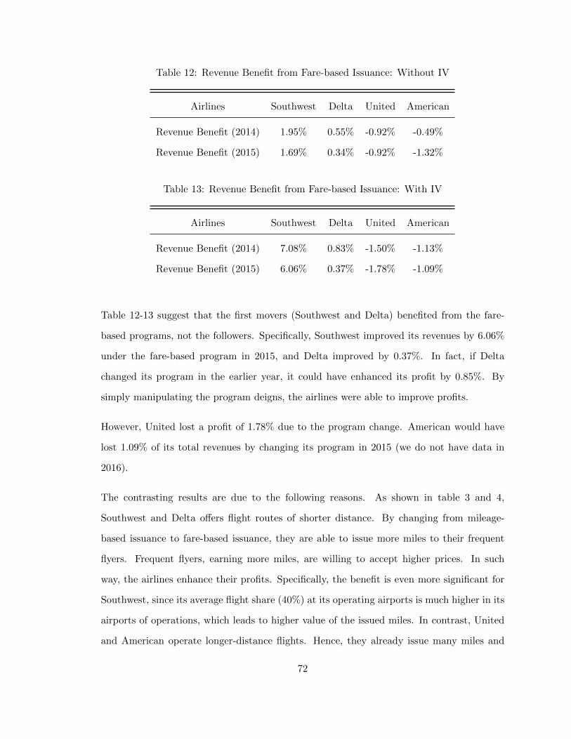
Table 12: Revenue Benefit from Fare-based Issuance: Without IV

Airlines Southwest Delta United American

Revenue Benefit (2014) 1.95% 0.55% -0.92% -0.49%

Revenue Benefit (2015) 1.69% 0.34% -0.92% -1.32%

Table 13: Revenue Benefit from Fare-based Issuance: With IV

Airlines Southwest Delta United American

Revenue Benefit (2014) 7.08% 0.83% -1.50% -1.13%

Revenue Benefit (2015) 6.06% 0.37% -1.78% -1.09%

Table 12-13 suggest that the first movers (Southwest and Delta) benefited from the fare-

based programs, not the followers. Specifically, Southwest improved its revenues by 6.06%

under the fare-based program in 2015, and Delta improved by 0.37%. In fact, if Delta

changed its program in the earlier year, it could have enhanced its profit by 0.85%. By

simply manipulating the program deigns, the airlines were able to improve profits.

However, United lost a profit of 1.78% due to the program change. American would have

lost 1.09% of its total revenues by changing its program in 2015 (we do not have data in

2016).

The contrasting results are due to the following reasons. As shown in table 3 and 4,

Southwest and Delta offers flight routes of shorter distance. By changing from mileage-

based issuance to fare-based issuance, they are able to issue more miles to their frequent

flyers. Frequent flyers, earning more miles, are willing to accept higher prices. In such

way, the airlines enhance their profits. Specifically, the benefit is even more significant for

Southwest, since its average flight share (40%) at its operating airports is much higher in its

airports of operations, which leads to higher value of the issued miles. In contrast, United

and American operate longer-distance flights. Hence, they already issue many miles and

72

cannot benefit from changing to the new program.

Issuing more miles lead to higher profits. However, it remains unclear whether the results

hold when the number of issued miles approaches infinity, since the current analysis is

limited by the range of issued miles in the data. It is likely that as more miles are put

into circulation, a redemption probability that is too low leads to reduced values of miles

eventually.

2.6. Conclusions

We have four conclusions:

First, frequent flyer miles carry values to customers only when they can be put into good

use. Both the award capacity and award choices have a significant impact on the value

of miles. At the average level of award capacity, a mile is valued between 2-4 cents in

customers’ decisions, which can be two times higher than the Tripadvisor.com benchmark.

Southwest miles are most valuable, yielding around 6 cent per mile; JetBlue miles are least

valuable at 1 cent per mile. Even within the same airlines, miles are valued differently by

customers from different regions. For example, an American Airlines mile is worth 6.52 cent

at JFK but is worthless at BUR.

Second, a redeemed mile is valued differently from an issued mile by customers. The average

value of a mile at redemption is 2.35 cent. Redeemed miles have higher values when they

are used from origin airports where their issuer provides more future flight options, and

to destination airports with higher flight fares. For instance, an American Airlines mile

redeemed from CLT to CVG is worth 3.25 cent; in comparison, if it is redeemed from BWI

to OAK, the value decreases to 1.92 cent, due to lower market share at BWI and lower

prices toward Oakland.

Third, compared to the objective value of miles, customers over-evaluate miles both at

issuance (by 139%) and redemption (by 346%). The huge difference may result from over-

73

confidence of the redemption value and redemption probability.

Finally, airlines can improve profits (up to 7%) by simply manipulating program designs.

Specifically, short-distance carriers (Southwest and Delta) benefit from fare-based issuance

of miles, while long-distance carriers (American and United) find mileage-based issuance

more attractive. Airlines should pay careful attention to their flight attributes and design

its loyalty programs in order to issue more miles into circulation.

74

: Bibliography

[1] BoardingArea, 2014. Value of miles & points.

Retrieved July 10, 2015, http://onemileatatime.boardingarea.com/value-miles-points/.

[2] BoardingArea. 2015. Hotel reward availability: Who does it best? Retrieved July 10, 2015,

http://blog.wandr.me/2015/01/best-hotel-rewards-program-availability/.

[3] Brunger, W. G. 2013. How should revenue management feel about frequent flyer programs.

Journal of Revenue & Pricing Management. 12(1) 1-7.

[4] Dreze, X., J. C. Nunes. 2004. Using combined-currency prices to lower consumers’ perceived

cost. Journal of Marketing Research. 41(1) 59-72.

[5] Hsee, C. K., F. Yu, J. Zhang, Y. Zhang. 2003. Medium maximization. Journal of Consumer

Research. 30(1) 1-14.

[6] Kivetz, R., O. Urminsky, Y. Zheng. 2006. The goal-gradient hypothesis resurrected: Purchase

acceleration, illusionary goal progress, and customer retention. Journal of Marketing Research.

43(1) 39-58.

[7] Nunes, J. C., X. Dreze. 2006. The endowed progress effect: How artificial advancement increases

effort. Journal of Consumer Research. 32(4) 504-512.

[8] Raghubir, P., J. Srivastava. 2002. Effect of face value on product valuation in foreign currencies.

Journal of Consumer Research. 29(3) 335-347.

[9] Sayman, S., S. J. Hoch. 2014. Dynamics of price premiums in loyalty programs. European

Journal of Marketing. 48(3) 617-640.

[10] Stourm, V., E. T. Bradlow, P. S. Fader. 2015. Stockpiling points in linear loyalty programs.

Working paper, American Marketing Association.

[11] van Osselaer, S. M. J., J. W. Alba, P. Manchanda. 2004. Irrelevant information and mediated

intertemporal choice. Journal of Consumer Psychology. 14 (3) 257-70.

[12] Wertenbroch, K., D. Soman, A. Chattopadhyay. 2007. On the perceived value of money: The

75

reference dependence of currency numerosity effects. Journal of Consumer Research. 34(1)

1-10.

76

CHAPTER 3 : THE EFFECT OF DYNAMIC PRICING ON UBER’S

DRIVER-PARTNERS

We study the effects of dynamic pricing (so-called “surge pricing”) on Uber’s driver-partners.

Using a natural experiment arising from a surge pricing service outage for a portion of Uber’s

driver-partners over 10 major cities, and a difference-in-differences approach, we study the

effect of showing the surge heatmap 1) on drivers’ decisions to relocate to areas with higher

or lower prices and 2) on drivers’ earnings. We demonstrate that the ability to see the

surge heatmap has a statistically significant impact on both outcomes, explaining 10%-60%

of Uber drivers’ self-positioning decisions and attracting drivers toward areas with higher

surge prices, and increasing drivers’ earnings on surged trips by up to 70%.

3.1. Introduction

The study of dynamic pricing at Uber and within other ride-sharing platforms has typically

focused at an aggregate spatial level. This literature argues that rider-side pricing influences

the number of riders wishing to take trips (10), and driver-side pricing along with this

volume of riders taking trips influences the availability of drivers to successfully fulfill those

trips (5; 8). This literature then seeks to understand how different pricing methodologies

influence outcome like social welfare and the firm’s profit (8; 3).

The way in which pricing influences availability of drivers, however, is multifaceted: This

influence may occur through (1) changing the numbers of drivers driving somewhere within

the city (by influencing drivers’ decisions to sign up for Uber, or when to drive within the

week); and (2) where to drive conditioned on having chosen to drive. The influence of price

on where drivers drive if it indeed occurs, presumably happens through influencing drivers’

expectations about the price and trip volume at a particular location in the near future.

This influence on expectations may be effected through the average or typical price at a

particular location and time of day/week as observed over longer timescales (days or weeks),

and/or through the signaling effect of the current price on price and trip volume in other

77

nearby locations over a much shorter timescale (minutes or hours).

Much of this influence (when to drive, and influencing where to drive through average price)

can be effected by driver pricing schemes that are not dynamic. These could be effected

by changing the driver-side price slowly over time, perhaps advertising in advance what

the driver-side prices would be. Only the short-run signaling effect need be effected via a

dynamic pricing scheme. Moreover, anecdotal evidence is ambiguous on the whether this

short-run signaling effect is significant. While some drivers do report responding to the

real-time value of the surge multiplier, others advise against “chasing surge” (6), suggesting

that variability in surge prices and the costs of changing one’s location makes reacting too

strongly to surge prices disadvantageous.

If the short-run effect of dynamic pricing on signaling is not significant, and all of driver-side

pricing’s effect on driver availability occurs through slower timescales, one could imagine an

alternate design from today’s ride-sharing platforms using a static or slowly-varying driver-

side pricing scheme intended to replicate the average-case dynamics of today’s dynamic

scheme, together with a more dynamic rider-side pricing scheme that reacts to short-term

fluctuations in demand. This would be of particular interest because the dynamic nature of

Uber’s surge pricing has generated a great deal of attention, particularly within the popular

press (18? ; 12), but also within the academic literature (3).

On the other hand, if the short-run effect of dynamic pricing on signaling is significant,

then this alternatively suggests that supply-side dynamic pricing schemes can be useful

mechanisms for reducing friction in labor markets, and may have implications for other

two-sided markets where labor is constrained in space, in time, by skill-set, or by specialty.

Moreover, while intertemporal substitution of labor has been studied in ridesharing and

taxi markets in the context of income targeting (9) and long-run supply elasticity (13),

spatial elasticity in ridesharing markets has been under-investigated. The most closely-

related paper to our knowledge (4) estimates taxi drivers’ “spatial equilibrium” behavior

78

in NYC and the impact of pricing policy. While both their papers and ours study similar

settings using MNL models, their paper focuses mainly on the impact of ex-ante beliefs

of location values on drivers’ movement decisions, without the consideration of dynamic

pricing or other real-time information. In contrast, our paper focuses on the impact of

real-time spatial pricing on drivers’ decisions.

In this paper, we study this question empirically using a natural experiment in which Uber’s

surge prices ceased to be visible for drivers using phones on the iOS operating system in 10

of its largest markets. Using a difference-in-differences approach (2; 7), and controlling for

a number of confounding factors, we provide evidence that dynamic surge prices do have a

significant effect on drivers’ self-positioning decisions, causing drivers to drive toward nearby

areas with higher surge values. We also show that having access to real-time information

from the surge heatmap increased earnings for unaffected drivers, controlling for systematic

differences between drivers using iOS and Android phones. This suggests that dynamic

pricing is useful as a real-time signaling tool for reducing frictions in the ridesharing labor

market, better aligning drivers’ locations with riders’ desire to take trips.

The use of a natural experiment is critical for answering the question of whether information

provided by the surge heatmap causes drivers to relocate over short timescales. This is

because endogeneity is particularly problematic for understanding causality in the surge

heatmap’s relationship to drivers’ repositioning decisions. Drivers learn the areas of their

city where demand tends to outstrip supply, and they tend to drive toward those areas to

benefit from shorter wait times between trips and higher surge multiplies. If drivers make

these repositioning decisions exclusively based on their private knowledge, and not based on

the real-time information present in the surge heatmap, then we would nevertheless expect

to see a correlation between the surge heatmap’s multipliers and drivers’ repositioning

decisions. Disentangling this effect from the causal impact of the heatmap on drivers’

movements would be challenging.

The natural experiment allows us to disentangle these effects. Using a difference-in-differences

79

approach within a multinomial logit discrete choice model, we can compare the relocation

decisions and earnings on the outage weekend among iOS drivers with an estimate for what

these decisions and earnings would have been without the outage based on data from other

weekends on all drivers, and data from the outage weekend from unaffected Android drivers.

In addition to the work cited above on ridesharing, our work is also related to the larger

literature on spatial mobility in labor markets (16), and in particular to empirical analyses

of the spatial elasticity of labor supply (15, Chapter 9,), (14). While related, this literature

has typically focused on spatial mobility over longer time and spatial scales. More generally,

our work can be viewed within the larger literature on informational and physical frictions

in labor markets (16). This literature often focuses on search (17), and within this context,

the surge heatmap can be seen as an aid that reduces the cost of search for drivers in the

ridesharing market.

The rest of the paper is organized as follows. Section 2 starts with a description of method-

ology, including Uber’s pricing system, the natural experiment, a driver behavior model

and its difference-in-differences estimation. Section 3 dives into the estimation results and

their implications of the effects of dynamic pricing on both driver movement and earnings.

Finally, Section 4 summarizes with conclusions.

3.2. Methodology

We will analyze a natural experiment in which an outage made the surge heatmap unavail-

able for drivers using the iOS driver app in many of Uber’s largest cities over one weekend.

To analyze this experiment, we use a multinomial logit model over the driver’s direction of

motion. This MNL model uses utility determined by a factor model over the change in surge

multiplier in each direction of movement, the visibility of the surge heatmap, the driver’s

operating system, a time indicator controlling for changes in driver movement between the

outage and non-outage weeks, and driver covariates intended to control for differences in

behavior between iOS and Android drivers. Under the assumption of zero coefficients for

80

the two-way interaction between the operating system and time terms, and for the three-

way interaction between operating system, time, and surge multiplier change, this analysis

is able to identify the impact of making the surge heatmap visible to drivers, with results

presented in section 3.3.

We now describe this methodology in detail, first summarizing background on Uber’s surge

pricing system (section 3.2.1), then summarizing the MNL model (section 3.2.3) and factor

utility model (section 3.2.4), and finally describing the natural experiment and how the

MNL and factor utility model was applied to analyze it (section 3.2.5).

3.2.1. Background on Uber’s Surge Pricing System

Uber operates a two-sided market in which individuals wishing to take a trip (“riders”)

are matched with other individuals willing to drive them for a fee (“drivers”). The rider

requests a trip via a smartphone application, the “rider app”, and the driver accepts or

rejects dispatch requests via another smartphone application, the “driver app”. We focus

on the UberX service in which a single rider or party of riders occupies a car, and do not

discuss other Uber products.

At the time when the natural experiment we analyze occurred, both the price paid by the

rider and the fee earned by the driver for participating in the UberX service were both set

via a “surge multiplier” and the “unsurged fare”. The unsurged fare was computed from the

time and distance traveled by the driver with the rider in the vehicle via a fixed city-specific

linear functon, while the surge multiplier was computed dynamically as described below.

The rider price was then obtained by multiplying the unsurged fare by the surge multiplier.

The driver’s earnings for the trip were then calculated by removing a fixed commission from

the total amount paid by the rider.

Cities are partitioned into non-overlapping uniform hexagons, each with an edge length of

0.2 miles (0.32km). Each hexagon is assigned its own surge multiplier, which is recalculated

every 2 minutes, and is applied to all trips starting in that hexagon over that two minute

81

period.

Uber sets surge multipliers dynamically and algorithmically. This algorithm sets surge

multiplier based on the number of riders in the process of using the rider app to make trip

requests in a geographically localized area, the number of driver partners in or near that

area who have made themselves available to conduct trips via the driver app, as well as

some additional factors.

The surge pricing algorithm is designed to balance supply and demand in real time: when

the number of trip requests seem likely to exceed the number of trips that nearby cars can

fulfill, it increases the surge multiplier to ensure that only riders that place a high value on

taking a trip do so, and to attract drivers to the undersupplied area.

It is reasonable to expect that drivers would prefer to be in hexagons with high surge

multipliers, both because a higher surge multiplier results in a larger payment to the driver

holding fixed a trip’s time and distance, and because a higher surge multiplier typically

indicates that the ratio of riders to drivers is high and thus a driver’s waiting time for a

trip will be short. Uber also prefers drivers to move to areas with higher surge multipliers,

because their presence in high-demand areas allows more riders to take trips with lower

waiting times.

To support this movement toward surging areas, the driver app shows a visualization

called the “surge heatmap” (see Figure 7) that displays the current surge multiplier in

each hexagon. Drivers can see this surge heatmap when they have indicated in the driver

app they will consider dispatch requests and they are not currently servicing a request.

We call such drivers in the “open” state. Drivers who are unwilling to consider dispatch

requests (either because they have indicated so in the app, or the app is turned off) are

considered to be in the “offline” state. Once a rider is matched with an open driver, the

driver is given directions on where to meet the rider and the surge heatmap is no longer

visible. We call drivers on their way to pick up a rider “en route,” and drivers who are

82

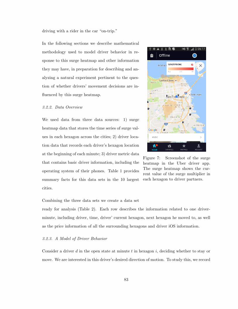
driving with a rider in the car “on-trip.”

Figure 7: Screenshot of the surgeheatmap in the Uber driver app.The surge heatmap shows the cur-rent value of the surge multiplier ineach hexagon to driver partners.

In the following sections we describe mathematical

methodology used to model driver behavior in re-

sponse to this surge heatmap and other information

they may have, in preparation for describing and an-

alyzing a natural experiment pertinent to the ques-

tion of whether drivers’ movement decisions are in-

fluenced by this surge heatmap.

3.2.2. Data Overview

We used data from three data sources: 1) surge

heatmap data that stores the time series of surge val-

ues in each hexagon across the cities; 2) driver loca-

tion data that records each driver’s hexagon location

at the beginning of each minute; 3) driver metric data

that contains basic driver information, including the

operating system of their phones. Table 1 provides

summary facts for this data sets in the 10 largest

cities.

Combining the three data sets we create a data set

ready for analysis (Table 2). Each row describes the information related to one driver-

minute, including driver, time, driver’ current hexagon, next hexagon he moved to, as well

as the price information of all the surrounding hexagons and driver iOS information.

3.2.3. A Model of Driver Behavior

Consider a driver d in the open state at minute t in hexagon i, deciding whether to stay or

move. We are interested in this driver’s desired direction of motion. To study this, we record

83

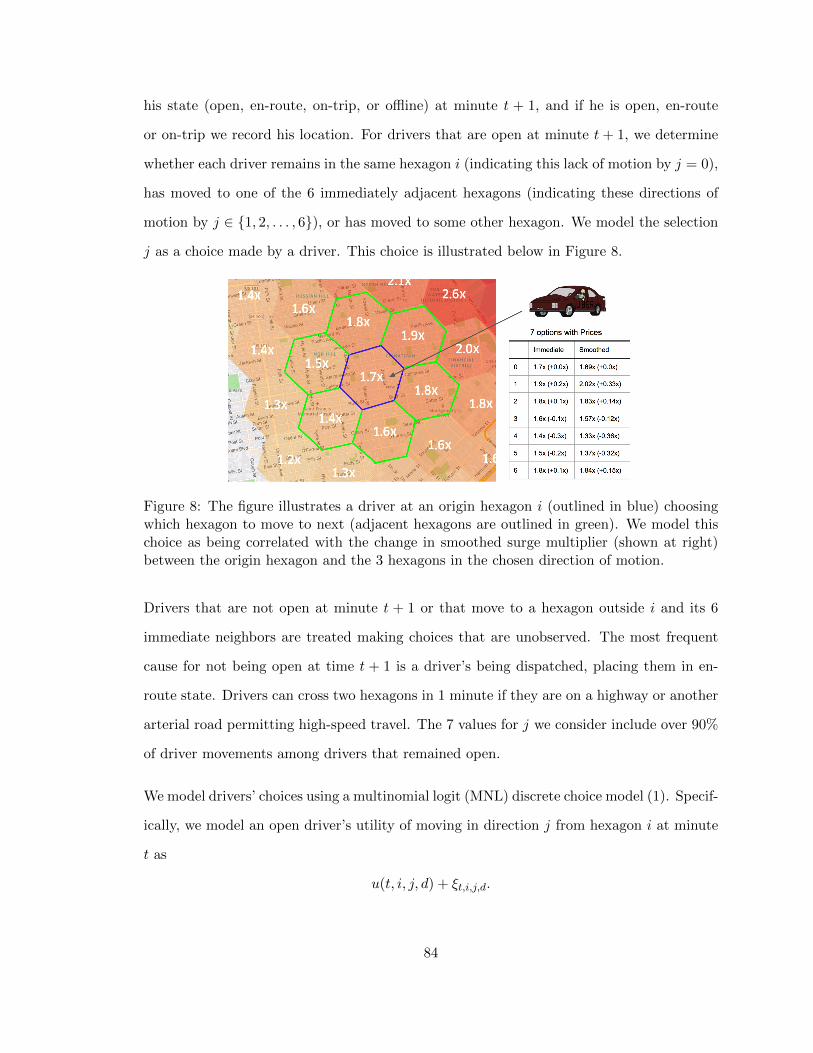
his state (open, en-route, on-trip, or offline) at minute t + 1, and if he is open, en-route

or on-trip we record his location. For drivers that are open at minute t + 1, we determine

whether each driver remains in the same hexagon i (indicating this lack of motion by j = 0),

has moved to one of the 6 immediately adjacent hexagons (indicating these directions of

motion by j ∈ {1, 2, . . . , 6}), or has moved to some other hexagon. We model the selection

j as a choice made by a driver. This choice is illustrated below in Figure 8.

Figure 8: The figure illustrates a driver at an origin hexagon i (outlined in blue) choosingwhich hexagon to move to next (adjacent hexagons are outlined in green). We model thischoice as being correlated with the change in smoothed surge multiplier (shown at right)between the origin hexagon and the 3 hexagons in the chosen direction of motion.

Drivers that are not open at minute t + 1 or that move to a hexagon outside i and its 6

immediate neighbors are treated making choices that are unobserved. The most frequent

cause for not being open at time t + 1 is a driver’s being dispatched, placing them in en-

route state. Drivers can cross two hexagons in 1 minute if they are on a highway or another

arterial road permitting high-speed travel. The 7 values for j we consider include over 90%

of driver movements among drivers that remained open.

We model drivers’ choices using a multinomial logit (MNL) discrete choice model (1). Specif-

ically, we model an open driver’s utility of moving in direction j from hexagon i at minute

t as

u(t, i, j, d) + ξt,i,j,d.

84

Here, ξt,i,j,d is an independent Gumbel distributed random variable. u(t, i, j, d) represents

the driver’s perceived utility of making movement direction j when in hexagon i at time t

for a driver with a set of driver features d. We will discuss the form of u(t, i, j, d) in detail

below.

While this model, conditioned on having an observation (which includes, for example, the

condition that the driver is not dispatched), and given a particular utility function, the

probability of observing choice j is,

P (j|t, i, d) =exp(u(t, i, j, d))∑6

j′=0 exp(u(t, i, j′, d)).

A number of factors may contribute to a driver’s choice of j. We are interested most

importantly in the causal effect of the surge multiplier, but also the confounding effect that

motion may be correlated with the surge multiplier because drivers tend to move toward

high-demand areas and high-demand areas tend to surge. To allow our model to capture

the dependence of motion on such factors, we include in our utility u(t, i, j, d) the difference

in smoothed surge multiplier ∆p(t, i, j) between the origin hexagon i and for the hexagon in

direction j. We will address possible confounding through the natural experiment discussed

below.

More precisely, the term ∆p(t, i, j) is computed by first computing a “smoothed” surge

multiplier for each hexagon, obtained by averaging the surge multipliers in the hexagons in

three concentric rings. This provides a smoothed surge price for the origin p(t, i) and for

the hexagons in the 6 directions p(t, j). Then ∆p(t, i, j) = p(t, j)−p(t, i) is the difference in

these prices. The values of the smoothed surge multipliers and corresponding ∆p(t, i, j) are

presented in the column ”Smoothed” in the table in Figure 8. The values in the “Immediate”

column are based on the non-smoothed surge multipliers from only a single hexagon. The

motivation of using smoothed multipliers is to capture the attraction of surged hexagons

that are further away than one ring. When we did not smooth multipliers, we saw similar

85

results on all metrics.

Another factor that may contribute to a driver’s choice of j is whether the heatmap was

visible when the driver was making his or her decision. This will be encoded through a

factor invisible(d, t), which takes a value of 0 for drivers d and times t for which the surge

heatmap was visible to open drivers (as is typical), and takes a value of 1 when the heatmap

is hidden, as it was in the outage in our natural experiment.

While we discuss in more detail the specific functional form assumed for u(t, i, j, d) in the

next section, and discuss assumptions following from that functional form there, we note

and briefly discuss assumptions we have made thus far:

A1. ξt,i,j,d are independent across t, i, j, d. This assumes implicitly and in particular that

driver d’s decisions are not directly influenced by other drivers in the immediate area.

It does, however, allow a driver’s decisions to be influenced indirectly by other nearby

drivers, through the impact their presence has on surge multipliers and waiting times.

A2. The dependence of u(t, i, j, d) on hexagon i and direction j is only through the price

difference ∆p(t, i, j).

A3. Drivers’ movement decisions are not influenced by surge multipliers further than the

4th ring of hexagons from their current hexagon. This is a distance of approximately

1.5 miles.

A4. Observations of drivers movements are censored independently of their unobserved

movement decisions.

A5. We assume that the probability distribution describing driver’s choices’ has the func-

tional form of an MNL model.

We now discuss the functional form of u(t, i, j, d) in detail.

86

3.2.4. The Utility Function

Without loss of generality, we normalize the utility of staying in the same hexagon, u(t, i, 0, d),

to be 0. The utility of moving in direction j, u(t, i, j, d), then is the change in the driver’s

utility relative to staying. To model the value of u(t, i, j, d) for j > 0, we use a factor model

containing the following features:

• the difference in surge multiplier ∆p(t, i, j) discussed above

• a collection of driver metrics that depend on d: the operating system, the driver’s age,

and the driver’s tenure on the Uber platform. We discuss and motivate these choices

below. We indicate these here in a generic way with a vector x(d) with components

xk(d), where k starts at 0.

• the binary indicator invisible(d, t) that is 1 if the heatmap is hidden to drivers and 0

otherwise

• a binary time indicator T (t). Within the analysis of the natural experiment, we will

apply our factor model to data collected over two weeks. This indicator will take the

value 1 for the week when the outage occurred, and 0 in the previous week.

This model has the following specific form:

u(t, i, j, d) = β0 + β1 ·∆p(t, i, j)

+ T (t) · [β2 + β3 · ·∆p(t, i, j)]

+ invisible(d, t)[β4 + β5 ·∆p(t, i, j)]

+∑k

xk(d) · [β6+3k ·+β7+3k ·∆p(t, i, j) + β8+3k · T (t) + β9+3k ·∆p(t, i, j) · T (t)]

(3.1)

The first row of coefficients includes a constant term β0, which one can interpret as the

value of moving out of the current hexagon if all other factors are 0 (recall that this utility

87

is the value for all j > 0, and the utility at j = 0 is fixed to 0). It also includes a term β1

that represents the desirability of moving toward increasing surge multiplier. The second

and third rows contains similar terms, but now interacted with the time indicator T (t) in

the second row and the surge visibility invisible(d, t) in the third. The fourth row also

contains similar terms interacted with each driver feature, and also the interaction of this

driver feature with the time indicator and the price difference.

Taken collectively, the sum β1 + β3 · T (t) + β5 · invisible(d, t) +∑

k(β7+3k + β9+3k · T (t)) ·

xk(d) represents the dependence of the utility to the surge multiplier gradient, including

both dependence due to causal factors (drivers being attracted to areas with higher surge

multiplier) and due to non-causal confounding factors (drivers wishing to move toward areas

that are good to drive in, that happen to also have higher surge gradients). The coefficient

of β5 determines how this sensitivity changes when the surge heatmap is hidden, and it is

on this coefficient that we will focus when using the natural experiment to understand the

causal relationship between the surge heatmap and driver movement.

We take note of the model form (3.1) as an assumption.

A6. We assume that drivers’ utility is modeled by the functional form (3.1).

3.2.5. Description of the Natural Experiment

During the weekend of November 4th to 6th in 2016, cities served by one of Uber’s data

centers suffered from a technical outage in the surge pricing system. These cities included

New York City, Boston, Chicago, Washington DC, and many other cities in the United

States and around the world. In the affected cities, drivers using the driver app on an iOS

phone (so-called “iOS drivers”) received a blank map with no surge information. Drivers

using the driver app on an Android phone (so-called “Android drivers”) could see the surge

heatmap as usual. The outage only affected iOS drivers’ ability to see the surge heatmap,

but did not change the way in which they were paid.

88

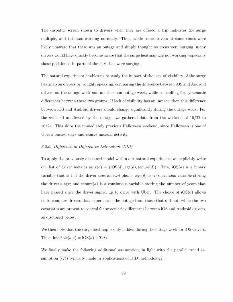
The dispatch screen shown to drivers when they are offered a trip indicates the surge

multiple, and this was working normally. Thus, while some drivers at some times were

likely unaware that there was an outage and simply thought no areas were surging, many

drivers would have quickly become aware that the surge heatmap was not working, especially

those positioned in parts of the city that were surging.

The natural experiment enables us to study the impact of the lack of visibility of the surge

heatmap on drivers by, roughly speaking, comparing the difference between iOS and Android

drivers on the outage week and another non-outage week, while controlling for systematic

differences between these two groups. If lack of visibility has an impact, then this difference

between iOS and Android drivers should change significantly during the outage week. For

the weekend unaffected by the outage, we gathered data from the weekend of 10/22 to

10/24. This skips the immediately previous Halloween weekend, since Halloween is one of

Uber’s busiest days and causes unusual activity.

3.2.6. Difference-in-Differences Estimation (DID)

To apply the previously discussed model within our natural experiment, we explicitly write

our list of driver metrics as x(d) = (iOS(d), age(d), tenure(d)). Here, iOS(d) is a binary

variable that is 1 if the driver uses an iOS phone; age(d) is a continuous variable storing

the driver’s age; and tenure(d) is a continuous variable storing the number of years that

have passed since the driver signed up to drive with Uber. The choice of iOS(d) allows

us to compare drivers that experienced the outage from those that did not, while the two

covariates are present to control for systematic differences between iOS and Android drivers,

as discussed below.

We then note that the surge heatmap is only hidden during the outage week for iOS drivers.

Thus, invisible(d, t) = iOS(d)× T (t).

We finally make the following additional assumption, in light with the parallel trend as-

sumption ((7)) typically made in applications of DID methodology.

89

A7. The coefficients on the interaction terms iOS(d) ·T (t) and iOS(d) ·T (t) ·∆p(t, i, j) are

0.

Assumption A7 assumes that the difference between iOS and Android drivers stays the same

week over week (except for the outage), and as we change the surge multiplier gradient

∆p(t, i, j). To help ensure that A7 is met, we include age(d) and tenure(d) and their

interactions with T (t), ∆p(t) and T (t) ·∆p(t) in our regression. This is discussed in more

detail in the next section.

Applying these three modeling choices to the utility model (3.1), we obtain:

u(t, i, j, d) = β0 + β1 ·∆p(t, i, j)

+ T (t) · [β2 + β3 ·∆p(t, i, j)]

+ invisible(d, t) · [β4 + β5 ·∆p(t, i, j)]

+ tenure(d) · [β6 + β7 ·∆p(t, i, j) + β8 · T (t) + β9 ·∆p(t, i, j) · T (t)]

+ age(d)[β10 + β11 ·∆p(t, i, j) + β12 · T (t) + β13 ·∆p(t, i, j) · T (t)]

+ iOS(d) · [β14 + β15 ·∆p(t, i, j)]

To estimate the model parameters, we use maximum likelihood estimation with the likeli-

hood implied by this factor model for the utility and the MNL model over driver decisions

j. To create confidence intervals and perform hypothesis tests, we use a bootstrapping

approach (11).

Within this model and estimation method, the sensitivity to the surge gradient is given by

β1 + β3 · T (t) + β5 · invisible(d, t) + β7 · tenure(d) + β9 · tenure(d) · T (t)+

β11 · age(d) + β13 · age(d) · T (t) + β15 · iOS(d).

(3.2)

With this in mind, we wish to test the following hypotheses about this sensitivity in our

analysis:

90

• that equation (3.2) is positive (indicating that drivers tend to move toward surge) for

typical values of T (t), tenure(d), age(d), and iOS(d) when invisible(d, t) = 0

• β5 is negative, showing that sensitivity of movement to surge is reduced when the

heatmap is not visible

• that equation (3.2) remains non-negative when invisible(d, t) = 1, showing that lack

of visibility of the surge heatmap does not cause drivers to move away from surge

Additionally, the coefficient associated with staying in the same place when ∆p = 0 is given

by

β0 + β2 · T (t) + β4 · invisible(d, t) + β6 · tenure(d) + β8 · tenure(d) · T (t)+

β10 · age(d) + β12 · age(d) · T (t) + β14 · iOS(d)

(3.3)

We wish to test the hypotheses that:

• this coefficient is negative for typical values of T (t), tenure(d), age(d), and iOS(d)

when invisible(d, t) = 0.

• this coefficient remains negative when invisible(d, t) = 1.

3.2.7. Differences Across Operating Systems and Time

Our approach relies on the assumption (A7) that iOS(d) · T (t) and iOS(d) · T (t) ·∆p(t, i, j)

have zero coefficients. To study this assumption, we study the difference between the two

weekends in our analysis, and the difference between iOS and Android drivers. We find

differences both across weekends and across groups, which are mitigated by controlling for

time, operating system, and other driver covariates in our analysis.

91

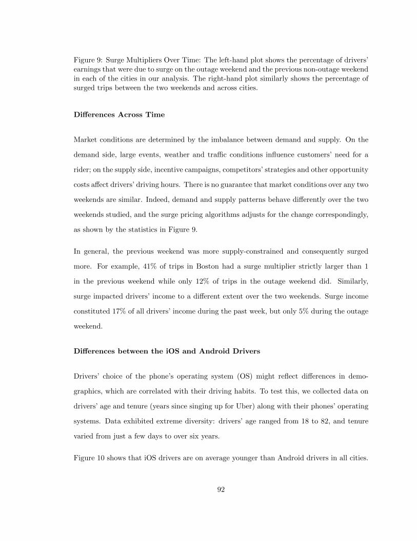
Figure 9: Surge Multipliers Over Time: The left-hand plot shows the percentage of drivers’earnings that were due to surge on the outage weekend and the previous non-outage weekendin each of the cities in our analysis. The right-hand plot similarly shows the percentage ofsurged trips between the two weekends and across cities.

Differences Across Time

Market conditions are determined by the imbalance between demand and supply. On the

demand side, large events, weather and traffic conditions influence customers’ need for a

rider; on the supply side, incentive campaigns, competitors’ strategies and other opportunity

costs affect drivers’ driving hours. There is no guarantee that market conditions over any two

weekends are similar. Indeed, demand and supply patterns behave differently over the two

weekends studied, and the surge pricing algorithms adjusts for the change correspondingly,

as shown by the statistics in Figure 9.

In general, the previous weekend was more supply-constrained and consequently surged

more. For example, 41% of trips in Boston had a surge multiplier strictly larger than 1

in the previous weekend while only 12% of trips in the outage weekend did. Similarly,

surge impacted drivers’ income to a different extent over the two weekends. Surge income

constituted 17% of all drivers’ income during the past week, but only 5% during the outage

weekend.

Differences between the iOS and Android Drivers

Drivers’ choice of the phone’s operating system (OS) might reflect differences in demo-

graphics, which are correlated with their driving habits. To test this, we collected data on

drivers’ age and tenure (years since singing up for Uber) along with their phones’ operating

systems. Data exhibited extreme diversity: drivers’ age ranged from 18 to 82, and tenure

varied from just a few days to over six years.

Figure 10 shows that iOS drivers are on average younger than Android drivers in all cities.

92

However, the ordering of their tenure differs across cities. Specifically, an average iOS drivers

has a longer tenure in Chicago (CHI), Boston (BOS), Washington D.C.(DC), Hong Kong

(HK), Moscow (MOW) and New Jersey (NJ), while an average android Android driver has

a longer tenure in New York (NYC), Atlanta (ATL), and Dallas (DAL).

Figure 10: Differences by Operating System: The figures show the tenure (left) and age(right) for iOS and Android Drivers, by city. Confidence intervals for the mean value areshown using the standard deviation of the sample mean.

To address these differences, we include tenure and age as covariates in our factor model,

their interactions with T (t) and ∆p(t, i, j), as well as the covariate iOS(d).

To further verify Assumption A7, we include in the appendix the results of a DiD analysis

with two regular weekends, which concludes that the coefficient on iOS(d) · T (t) ·∆p(t, i, j)

is 0.

3.3. Results

3.3.1. Impact of Surge on Driver Movement

Maximum likelihood estimates along with confidence intervals for model coefficients are

listed in Table 3. This table consists of two parts i) coefficients described in (3.3) that

represent the disutility of moving away from the current hexagon when ∆p(t, i, j) = 0; and

ii) coefficients described in (3.2) that represent the sensitivity of movement to the surge

gradient ∆p(t, i, j).

The table leads to several conclusions. First, it shows that in all cities, drivers incur a

93

disutility for driving out of the current hexagon (β0 < 0). Moreover, if they choose to drive

out, they derive a higher utility when they are driving toward hexagons with higher surge

values (β1 > 0). As the estimated value of β0 is large and negative compared to the other

coefficients in (3.3), if we compute (3.3) for another combination of factors the coefficient

will remain negative. A similar statement tends to hold for β1 and (3.2), although not

universally.

Second, surge information impacted driver movement, even when controlling for confound-

ing factors. Lack of visibility of the surge heatmap caused drivers to be less sensitive to

surge differences: β5 is significantly negative for all cities except for Washington D.C. and

New Jersey. Without the real-time knowledge of seeing the surge heatmap, iOS drivers had

a weaker signal of where to drive.

Table 3 quantifies the exogenous effect (β5) and endogenous effect (β1 + β3 + β15) of surge

for iOS drivers respectively. Therefore, we can measure the actual value of the real time

surge information on movement, out of the total surge-movement effect, as

e =−β5

β1 + β3 + β15

The exogenous effect of the heatmap accounted for 10% to 60% of the movement effect

(Figure 11). Consistent with discussion below, the effect is the lowest in the large cities

with more experienced drivers and higher surge (New York, Boston, Chicago).

Third, in all of the 10 cities, more experienced drivers were less likely to drive out of the

current hexagon (β6 < 0). Here are two potential explanations: 1) experienced drivers

understood that real-time demand conditions may change rapidly, and an imbalance that

was causing surge may indeed dissipate in the 2 minutes that pass between surge calcula-

tions. For this reason, they chase surge less often than inexperienced drivers; 2) experienced

drivers, afraid of being dispatched out of a low-surge hexagon, turned off their Open status

(go Offline) to be indispatchable, then drive toward high-surge hexagon and become Open

94

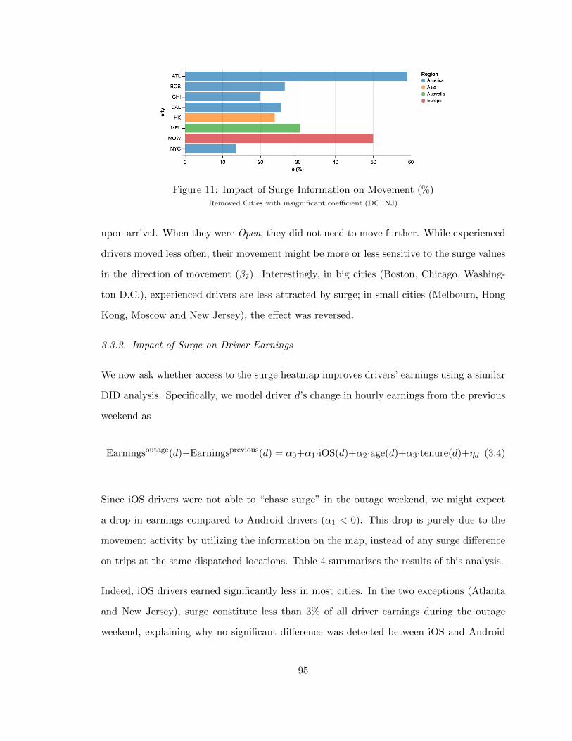
Figure 11: Impact of Surge Information on Movement (%)Removed Cities with insignificant coefficient (DC, NJ)

upon arrival. When they were Open, they did not need to move further. While experienced

drivers moved less often, their movement might be more or less sensitive to the surge values

in the direction of movement (β7). Interestingly, in big cities (Boston, Chicago, Washing-

ton D.C.), experienced drivers are less attracted by surge; in small cities (Melbourn, Hong

Kong, Moscow and New Jersey), the effect was reversed.

3.3.2. Impact of Surge on Driver Earnings

We now ask whether access to the surge heatmap improves drivers’ earnings using a similar

DID analysis. Specifically, we model driver d’s change in hourly earnings from the previous

weekend as

Earningsoutage(d)−Earningsprevious(d) = α0+α1·iOS(d)+α2·age(d)+α3·tenure(d)+ηd (3.4)

Since iOS drivers were not able to “chase surge” in the outage weekend, we might expect

a drop in earnings compared to Android drivers (α1 < 0). This drop is purely due to the

movement activity by utilizing the information on the map, instead of any surge difference

on trips at the same dispatched locations. Table 4 summarizes the results of this analysis.

Indeed, iOS drivers earned significantly less in most cities. In the two exceptions (Atlanta

and New Jersey), surge constitute less than 3% of all driver earnings during the outage

weekend, explaining why no significant difference was detected between iOS and Android

95

drivers’ earnings in these two areas.

On average, the absence of surge information reduced driver earnings by 20 to 80 cents

per hour. This amount does not seem striking, constituting only 1% to 4% of drivers’

total earnings (Figure 12). However, recall: 1) the outage did not change the surged

earnings the drivers could get; 2) surged earnings only constituted 2% to 12% of all driver

earnings, i.e., 40 cents to $3 per hour depending on the city. In fact, dividing the earnings’

difference (α1) due to the outage by the total surged earnings, we can caliberate the effects

of self-positioning on surge earnings, which ranges from 10% to as high as 70% (Figure 13).

The absence of the heatmap reduced driver earnings in the small cities the most, possibly

because these drivers had less experience and they relied more heavily on the heatmap to

make positioning decisions.

Figure 12: Effects of Self-Positioning on Total Earnings (%)

Removed Cities with insignificant coefficient (ATL, HK, NJ)

Figure 13: Effects of Self-Positioning on Surged Earnings (%)

Removed Cities with insignificant coefficient (ATL, HK, NJ)

96

3.4. Conclusions

This paper studies the short-run effect of dynamic pricing on Uber’s driver partners’ self-

positioning decisions and earnings. We first built up a driver positioning model in a Multi-

nomial Logit setup. Then we used data on a natural experiment covering 135,800 active

drivers over two weekends and performed a difference-in-differences estimation that resolved

endogeneity issues. The results suggest drivers rely heavily on the real-time dynamic pricing

information to make self-positioning decisions, and the effect is lower (10% 30%) in big cities

with professional drivers and higher (30% -60%) in small cities and with less experienced

drivers. By utilizing this information, drivers can identify potential earning opportunities

and significantly improve their surged earnings by up to 70%.

The results imply strong evidence that dynamic pricing is useful as a real-time signaling

tool for drivers to make self-positioning decisions that aligns with rider’s willingness to pay,

reducing frictions in the ride-sharing labor market, better aligning drivers locations with

riders desire to take trips.

97

: Bibliography

[1] S. P. Anderson, A. De Palma, and J. F. Thisse. Discrete choice theory of productdifferentiation. MIT press, 1992.

[2] O. C. Ashenfelter and D. Card. Using the longitudinal structure of earnings to estimatethe effect of training programs, 1984.

[3] S. Banerjee, R. Johari, and C. Riquelme. Pricing in ride-sharing platforms: A queueing-theoretic approach. In Proceedings of the Sixteenth ACM Conference on Economics andComputation, pages 639–639. ACM, 2015.

[4] N. Buchholz. Spatial equilibrium, search frictions and efficient regulation in the taxiindustry. Technical report, Technical report, University of Texas at Austin, 2015.

[5] G. P. Cachon, K. M. Daniels, and R. Lobel. The role of surge pricing on a service plat-form with self-scheduling capacity. Manufacturing & Service Operations Management,19(3):368–384, 2017.

[6] H. Campbell. Advice for new uber drivers — don’t chase thesurge!, 2017. URL https://maximumridesharingprofits.com/

advice-new-uber-drivers-dont-chase-surge/.

[7] D. Card. The impact of the mariel boatlift on the miami labor market. ILR Review,43(2):245–257, 1990.

[8] J. C. Castillo, D. Knoepfle, and G. Weyl. Surge pricing solves the wild goose chase.In Proceedings of the 2017 ACM Conference on Economics and Computation, pages241–242. ACM, 2017.

[9] M. K. Chen and M. Sheldon. Dynamic pricing in a labor market: Surge pricing andflexible work on the uber platform. In EC, page 455, 2016.

[10] P. Cohen, R. Hahn, J. Hall, S. Levitt, and R. Metcalfe. Using big data to estimateconsumer surplus: The case of uber. Technical report, National Bureau of EconomicResearch, 2016.

[11] B. Efron. Bootstrap methods: another look at the jackknife. In Breakthroughs instatistics, pages 569–593. Springer, 1992.

[12] M. Goncharova. Ride-hailing drivers are slaves to the surge. 2017.

[13] J. V. Hall and A. B. Krueger. An analysis of the labor market for ubers driver-partnersin the united states. ILR Review, page 0019793917717222, 2015.

[14] J. F. Madden. An empirical analysis of the spatial elasticity of labor supply. In Papersof the Regional Science Association, volume 39, pages 157–171. Springer, 1977.

98

[15] A. Manning. Monopsony in motion: Imperfect competition in labor markets. PrincetonUniversity Press, 2003.

[16] P. S. Morrison. Unemployment and urban labour markets. Urban Studies, 42(12):2261–2288, 2005.

[17] R. Rogerson, R. Shimer, and R. Wright. Search-theoretic models of the labor market:A survey. Journal of economic literature, 43(4):959–988, 2005.

[18] N. Scheiber. How uber uses psychological tricks to push its drivers’ buttons. 2017.

Appendix: DID Model without Driver Metrics

We also included a DID model with fewer predictors. The results are summarized in Table5. Similarly, the model shows significant effects of the heatmap (iOS · week · ∆p) for allcities except for Washington DC and New Jersey.

DID Model of Two Regular Weekends

Our conclusion of the impact of dynamic pricing on driver movement hinges on AssumptionA7 (The Parallel Trend Assumption), i.e., iOS and Android drivers do not exhibit diversetrends in their sensitivity to prices, after controlling for different driver metrics (Age andTenure). To test this theory, we ran a similar DID analysis over two regular weekends,including the previous weekend in the main analysis (10/22 to 10/24) and the weekendbefore (10/15 to 10/17).

The results are summarized in Table 6. For almost all cities, the coefficient on iOS ·week ·pis insignificant at 95% confidence interval with mixed signs. The only exception is NewJersey, which had no significant results in the outage weekend analysis. This could possiblydue to random noise, or some experiment running in the city that had different builts inthe platforms.

99

Table 14: Summary Statistics for 10 Largest Cities.

City Metrics Driver Metrics

Trips Surge Percentage Average Surge iOS Drivers iOS Supply Hours Android Drivers Android Supply Hours

NYC754753 0.16 1.07 35057 17539 34982 18627BOS381959 0.13 1.02 8012 8838 7533 9600CHI534294 0.19 1.07 11010 11496 13690 11539DC 478290 0.07 1.01 5279 2251 5293 2550ATL215983 0.03 1.01 4769 6512 7902 4198DEN152086 0.17 1.13 2794 2684 4026 1996MEL214744 0.15 1.05 6465 3891 4002 6104HK117862 0.11 1.06 2269 2921 7401 982

MOW137170 0.07 1.06 1263 5010 6987 1068NJ 232656 0.08 1.06 8009 4918 7967 3463

This table provides statistics on city pricing metrics and driver supply metrics related to trips and driver movements taken in the 10 citiesbetween November 4, 2016 and November 6, 2016. The surge percentage and average surge values are based on the surge data. The numberof active iOS and Android drivers and their supply hours (number of hours on the Uber platform) are collected through the movement data.

100

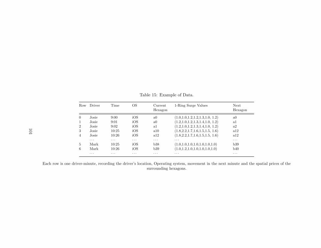
Table 15: Example of Data.

Row Driver Time OS CurrentHexagon

1-Ring Surge Values NextHexagon

0 Josie 9:00 iOS a0 (1.0,1.0,1.2,1.2,1.3,1.0, 1.2) a01 Josie 9:01 iOS a0 (1.2,1.0,1.2,1.3,1.4,1.0, 1.2) a12 Josie 9:02 iOS a1 (1.2,1.0,1.2,1.3,1.4,1.0, 1.2) a23 Josie 10:25 iOS a10 (1.8,2.2,1.7,1.6,1.5,1.5, 1.6) a124 Josie 10:26 iOS a12 (1.8,2.2,1.7,1.6,1.5,1.5, 1.6) a12

· · · · · · · · · · · · · · · · · ·5 Mark 10:25 iOS b38 (1.0,1.0,1.0,1.0,1.0,1.0,1.0) b396 Mark 10:26 iOS b39 (1.0,1.2,1.0,1.0,1.0,1.0,1.0) b40

· · · · · · · · · · · · · · · · · ·

Each row is one driver-minute, recording the driver’s location, Operating system, movement in the next minute and the spatial prices of thesurrounding hexagons.

101

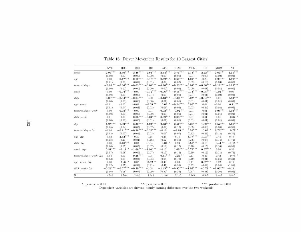
Table 16: Driver Movement Results for 10 Largest Cities.

NYC BOS CHI DC ATL DAL MEL HK MOW NJ

const −2.94∗∗∗ −2.46∗∗∗ −2.48∗∗∗ −2.64∗∗∗ −2.44∗∗∗ −2.71∗∗∗ −2.73∗∗∗ −2.52∗∗∗ −2.69∗∗∗ −3.11∗∗∗(0.00) (0.00) (0.00) (0.00) (0.00) (0.01) (0.01) (0.00) (0.00) (0.01)

age −0.00 −0.17∗∗∗ −0.10∗∗∗ 0.18∗∗∗ 0.32∗∗∗ 0.69∗∗∗ 1.01∗∗∗ −0.20 0.20∗∗∗ 1.19∗∗∗(0.01) (0.03) (0.01) (0.01) (0.02) (0.02) (0.02) (0.16) (0.03) (0.02)

tenured days −0.00 ∗∗ −0.06∗∗∗ −0.03∗∗∗ −0.04∗∗∗ −0.20∗∗∗ −0.23∗∗∗ −0.04∗∗∗ −0.36∗∗∗ −0.12∗∗∗ −0.15∗∗∗(0.00) (0.00) (0.00) (0.00) (0.00) (0.00) (0.00) (0.01) (0.01) (0.00)

week −0.00 −0.04∗∗∗ −0.00 −0.12∗∗∗ −0.06∗∗∗ −0.16∗∗∗ −0.14∗∗∗ −0.05∗∗∗ −0.02 ∗∗ −0.00(0.00) (0.01) (0.00) (0.01) (0.00) (0.01) (0.01) (0.01) (0.00) (0.01)

iOS 0.03∗∗∗ −0.04∗∗∗ −0.04∗∗∗ 0.00 −0.13∗∗∗ −0.03 ∗∗ 0.07∗∗∗ −0.04∗∗∗ 0.01 0.33∗∗∗(0.00) (0.00) (0.00) (0.00) (0.01) (0.01) (0.01) (0.01) (0.01) (0.01)

age · week −0.01 −0.03 −0.01 −0.05 ∗∗ 0.03 ∗ −0.24∗∗∗ 0.86∗∗∗ 0.04 −0.04 0.11 ∗∗(0.01) (0.04) (0.02) (0.02) (0.01) (0.04) (0.03) (0.24) (0.03) (0.03)

tenured days · week 0.00 −0.03∗∗∗ −0.00 −0.01 −0.02∗∗∗ 0.02 ∗∗ −0.01 0.01 0.04∗∗∗ −0.03∗∗∗(0.00) (0.00) (0.00) (0.00) (0.00) (0.01) (0.01) (0.01) (0.01) (0.01)

iOS · week −0.01 0.00 0.03∗∗∗ −0.04∗∗∗ 0.09∗∗∗ 0.08∗∗∗ 0.01 −0.01 −0.01 0.02 ∗(0.00) (0.01) (0.00) (0.01) (0.01) (0.01) (0.01) (0.01) (0.01) (0.01)

∆p 1.25∗∗∗ 1.99∗∗∗ 3.30∗∗∗ 1.97∗∗∗ 2.43∗∗∗ 2.57∗∗∗ 3.20∗∗∗ 1.69∗∗∗ 3.52∗∗∗ 5.61∗∗∗(0.05) (0.04) (0.07) (0.07) (0.09) (0.12) (0.09) (0.08) (0.08) (0.35)

tenured days ·∆p −0.04 −0.11∗∗∗ −0.36∗∗∗ −0.23∗∗∗ −0.12 −0.18 ∗ 0.51∗∗∗ 0.65 ∗ 0.76∗∗∗ 0.77 ∗(0.03) (0.03) (0.01) (0.03) (0.06) (0.07) (0.12) (0.27) (0.13) (0.30)

age ·∆p −0.02 −2.52∗∗∗ −0.30 0.15 −0.23 −0.16 3.77∗∗∗ 1.03∗∗∗ −1.44 −0.79(0.18) (0.21) (0.24) (0.16) (0.52) (0.31) (0.56) (0.06) (0.74) (1.72)

iOS ·∆p 0.10 0.18∗∗∗ 0.03 −0.04 0.34 ∗ 0.24 0.56∗∗∗ −0.10 0.44 ∗∗ −1.15 ∗(0.06) (0.05) (0.07) (0.07) (0.16) (0.17) (0.10) (0.15) (0.16) (0.53)

week ·∆p 0.31∗∗∗ −0.18 ∗ −1.66∗∗∗ −1.94∗∗∗ −0.10 1.09∗∗∗ −0.79∗∗∗ 0.57∗∗∗ 0.08 0.36(0.07) (0.08) (0.09) (0.07) (0.15) (0.13) (0.10) (0.12) (0.11) (0.71)

tenured days · week ·∆p 0.04 0.01 0.28∗∗∗ 0.05 0.41∗∗∗ 0.26 ∗∗ 0.11 −0.45 −0.42 −0.74 ∗(0.03) (0.05) (0.03) (0.05) (0.08) (0.10) (0.19) (0.31) (0.24) (0.34)

age · week ·∆p 0.00 1.44 ∗ 0.02 0.62 ∗∗ 0.43 0.03 −0.11 0.97∗∗∗ −1.22 −0.15(0.22) (0.67) (0.31) (0.21) (0.41) (0.30) (0.92) (0.02) (0.84) (1.88)

iOS · week ·∆p −0.29∗∗∗ −0.57∗∗∗ −0.39∗∗∗ −0.08 −1.45∗∗∗ −0.95∗∗∗ −1.05∗∗∗ −0.72 ∗ −1.03∗∗∗ −0.19(0.06) (0.08) (0.07) (0.09) (0.30) (0.20) (0.17) (0.31) (0.26) (0.93)

N 4.7e6 1.7e6 2.8e6 1.2e6 1.1e6 5.1e5 9.1e5 6.8e5 6.4e5 9.8e5

*: p-value = 0.05 **: p-value = 0.01 ***: p-value = 0.001Dependent variables are drivers’ hourly earning difference over the two weekends

102

Table 17: Driver Earnings Results for 10 Largest Cities.


const 0.23 −5.91∗∗∗ 0.61∗∗∗ −2.56∗∗∗ −2.42∗∗∗ 0.02 −5.24∗∗∗ 0.45∗∗∗ −0.36 ∗ −0.22(0.22) (0.26) (0.18) (0.17) (0.20) (0.31) (0.33) (0.09) (0.15) (0.18)

iOS −0.31 ∗ −0.57∗∗∗ −0.27 ∗∗ −0.24 ∗ 0.06 −0.61∗∗∗ −0.75∗∗∗ 0.01 −0.31 ∗∗ −0.03(0.14) (0.15) (0.10) (0.10) (0.12) (0.18) (0.19) (0.06) (0.10) (0.21)

age 0.01 0.63∗∗∗ 0.06 0.14∗∗∗ 0.16∗∗∗ 0.11 ∗ 0.90∗∗∗ 0.08 0.01 0.07(0.03) (0.06) (0.04) (0.03) (0.04) (0.05) (0.07) (0.12) (0.03) (0.07)

tenure −0.31∗∗∗ −1.17∗∗∗ −0.09 −0.32∗∗∗ −0.49∗∗∗ −0.46∗∗∗ −0.91∗∗∗ −0.19 ∗∗ −0.33∗∗∗ −0.17(0.07) (0.08) (0.05) (0.05) (0.07) (0.10) (0.15) (0.07) (0.07) (0.18)

N 3.4e4 1.5e4 2.7e4 2.2e4 1.4e4 9.4e3 9.6e3 1.0e4 7.8e3 2.1e4


Table 18: Driver Movement Results for 10 Largest Cities without Driver Metrics (Appendix)


const −2.94∗∗∗ −2.46∗∗∗ −2.48∗∗∗ −2.64∗∗∗ −2.43∗∗∗ −2.64∗∗∗ −2.71∗∗∗ −2.51∗∗∗ −2.69∗∗∗ −3.10∗∗∗(0.00) (0.00) (0.00) (0.00) (0.00) (0.00) (0.01) (0.00) (0.01) (0.00)

week 0.00 −0.03∗∗∗ −0.01 −0.12∗∗∗ −0.05∗∗∗ −0.19∗∗∗ −0.17∗∗∗ −0.04∗∗∗ −0.01 −0.01 ∗(0.00) (0.01) (0.00) (0.01) (0.00) (0.01) (0.01) (0.01) (0.01) (0.00)

iOS 0.03∗∗∗ −0.05∗∗∗ −0.05∗∗∗ −0.01 −0.17∗∗∗ −0.12∗∗∗ 0.10∗∗∗ −0.06∗∗∗ −0.01 0.31∗∗∗(0.00) (0.01) (0.00) (0.00) (0.01) (0.01) (0.01) (0.01) (0.01) (0.01)

iOS · week −0.01 0.00 0.03∗∗∗ −0.03∗∗∗ 0.13∗∗∗ 0.15∗∗∗ 0.01 −0.01 0.00 0.06∗∗∗(0.01) (0.01) (0.01) (0.01) (0.01) (0.01) (0.01) (0.01) (0.02) (0.01)

∆p 1.28∗∗∗ 2.02∗∗∗ 3.29∗∗∗ 1.80∗∗∗ 2.34∗∗∗ 2.42∗∗∗ 3.41∗∗∗ 1.67∗∗∗ 3.51∗∗∗ 5.86∗∗∗(0.04) (0.03) (0.06) (0.10) (0.16) (0.18) (0.13) (0.09) (0.12) (0.34)

iOS ·∆p 0.05 0.14 ∗ −0.10 −0.00 0.39 0.31 0.58∗∗∗ −0.09 0.48 ∗∗ −1.43∗∗∗(0.07) (0.06) (0.10) (0.12) (0.24) (0.24) (0.17) (0.13) (0.16) (0.36)

week ·∆p 0.31∗∗∗ −0.17 −1.64∗∗∗ −1.73∗∗∗ −0.06 1.11∗∗∗ −1.25∗∗∗ 0.56∗∗∗ 0.16 0.20(0.05) (0.10) (0.07) (0.11) (0.33) (0.23) (0.17) (0.15) (0.15) (0.53)

iOS · week ·∆p −0.24 ∗∗ −0.63∗∗∗ −0.31∗∗∗ −0.21 −1.65∗∗∗ −1.01∗∗∗ −0.86∗∗∗ −0.76 ∗∗ −0.90∗∗∗ 0.41(0.08) (0.16) (0.09) (0.13) (0.48) (0.24) (0.19) (0.25) (0.18) (0.56)

N 4.7e6 1.7e6 2.8e6 1.2e6 1.1e6 5.1e5 9.1e5 6.8e5 6.4e5 9.8e5


103

Table 19: Driver Movement Results over Two Regular Weekends. (Appendix)


const −2.80∗∗∗ −2.55∗∗∗ −2.53∗∗∗ −2.71∗∗∗ −2.62∗∗∗ −2.54∗∗∗ −2.63∗∗∗ −2.55∗∗∗ −2.69∗∗∗ −2.84∗∗∗(0.00) (0.00) (0.00) (0.00) (0.01) (0.01) (0.01) (0.00) (0.00) (0.01)

age −0.01 −0.07 ∗∗ 0.00 0.15∗∗∗ −0.15∗∗∗ 0.27∗∗∗ 0.13 ∗∗ −0.89∗∗∗ 0.25∗∗∗ 0.38∗∗∗(0.01) (0.02) (0.02) (0.02) (0.03) (0.04) (0.04) (0.21) (0.06) (0.02)

tenured days −0.02∗∗∗ −0.02∗∗∗ −0.06∗∗∗ −0.03∗∗∗ −0.01 ∗∗ −0.03 ∗∗ −0.02 ∗∗ −0.21∗∗∗ 0.00 −0.03∗∗∗

(0.00) (0.00) (0.00) (0.00) (0.00) (0.01) (0.01) (0.01) (0.01) (0.01)week −0.14∗∗∗ 0.10∗∗∗ 0.06∗∗∗ 0.08∗∗∗ 0.19∗∗∗ −0.10∗∗∗ −0.05∗∗∗ 0.03∗∗∗ −0.01 −0.26∗∗∗

(0.00) (0.01) (0.01) (0.00) (0.01) (0.01) (0.01) (0.00) (0.01) (0.01)iOS −0.00 −0.00 0.01 −0.01 0.05∗∗∗ 0.09∗∗∗ −0.01 0.05∗∗∗ 0.00 0.04∗∗∗

(0.00) (0.01) (0.00) (0.01) (0.01) (0.01) (0.01) (0.01) (0.01) (0.01)age · week 0.00 −0.12∗∗∗ −0.11∗∗∗ 0.03 ∗ 0.47∗∗∗ 0.41∗∗∗ 0.89∗∗∗ 0.70∗∗∗ −0.05 0.79∗∗∗

(0.01) (0.03) (0.03) (0.01) (0.03) (0.04) (0.05) (0.19) (0.07) (0.04)tenured days · week 0.01∗∗∗ −0.04∗∗∗ 0.03∗∗∗ −0.01 ∗ −0.19∗∗∗ −0.19∗∗∗ −0.03 ∗∗ −0.16∗∗∗ −0.12∗∗∗ −0.12∗∗∗

(0.00) (0.00) (0.00) (0.00) (0.00) (0.01) (0.01) (0.01) (0.01) (0.01)iOS · week 0.03∗∗∗ −0.04∗∗∗ −0.05∗∗∗ 0.01 −0.18∗∗∗ −0.11∗∗∗ 0.08∗∗∗ −0.09∗∗∗ 0.01 0.29∗∗∗

(0.00) (0.01) (0.01) (0.01) (0.01) (0.02) (0.01) (0.01) (0.01) (0.01)

∆p 1.14∗∗∗ 2.02∗∗∗ 2.86∗∗∗ 2.21∗∗∗ 2.62∗∗∗ 2.20∗∗∗ 3.68∗∗∗ 1.71∗∗∗ 2.44∗∗∗ 1.99∗∗∗(0.08) (0.05) (0.17) (0.19) (0.09) (0.23) (0.16) (0.25) (0.13) (0.38)

tenured days ·∆p −0.08 0.15∗∗∗ 0.64∗∗∗ 0.29 ∗ 0.59∗∗∗ −0.09 0.74∗∗∗ 0.09 0.69∗∗∗ 0.84∗∗∗(0.08) (0.05) (0.18) (0.13) (0.13) (0.18) (0.12) (0.41) (0.19) (0.20)

age ·∆p −0.24 −1.05 ∗∗ −4.47∗∗∗ −3.01 ∗∗ −0.44 −0.27 −7.86∗∗∗ 1.01∗∗∗ −2.77 ∗ −1.33(0.36) (0.34) (0.81) (1.07) (1.22) (0.14) (1.38) (0.18) (1.11) (0.77)

iOS ·∆p −0.00 0.16 ∗ 0.45 0.02 0.29 0.68 ∗ −0.12 0.03 1.06 ∗ −0.04(0.09) (0.08) (0.24) (0.21) (0.23) (0.34) (0.18) (0.58) (0.47) (0.55)

week ·∆p 0.13 0.04 0.61 ∗∗ −0.14 −0.04 0.41 −0.09 0.04 1.16∗∗∗ 3.85∗∗∗(0.09) (0.07) (0.22) (0.21) (0.15) (0.29) (0.26) (0.21) (0.17) (0.52)

tenured days · week ·∆p 0.03 −0.28∗∗∗ −0.95∗∗∗ −0.50∗∗∗ −0.79∗∗∗ −0.00 −0.20 0.33 0.00 0.12(0.08) (0.05) (0.17) (0.15) (0.15) (0.17) (0.10) (0.59) (0.24) (0.29)

age · week ·∆p 0.26 −1.46 ∗∗ 3.87∗∗∗ 3.24 ∗∗ 0.19 −0.09 11.69∗∗∗ 1.01∗∗∗ 1.76 −0.15(0.36) (0.47) (1.09) (1.19) (1.25) (0.09) (1.39) (0.17) (1.17) (0.46)

iOS · week ·∆p 0.06 0.00 −0.36 −0.02 −0.18 −0.13 0.42 −0.09 −0.66 −1.45 ∗(0.11) (0.11) (0.25) (0.20) (0.32) (0.26) (0.30) (0.54) (0.55) (0.72)

N 3.8e6 1.1e6 2.2e6 1.6e6 6.8e5 3.2e5 5.2e5 6.1e5 4.2e5 7.5e5


104

Documents

The Effect Of Dynamic Pricing And Revenue Management On