Purdue UniversityPurdue e-Pubs

Publications of the Ray W. Herrick Laboratories School of Mechanical Engineering

11-5-1996

The Effect of Edge Constraints on the SurfaceNormal Impedance of Layers of Elastic PorousMaterialsN.-M. ShiauFord Motor Company

W. DesmetKatholieke Universiteit Leuven

J Stuart BoltonPurdue University, bolton@purdue.edu

Follow this and additional works at: https://docs.lib.purdue.edu/herrick

This document has been made available through Purdue e-Pubs, a service of the Purdue University Libraries. Please contact epubs@purdue.edu foradditional information.

Shiau, N.-M.; Desmet, W.; and Bolton, J Stuart, "The Effect of Edge Constraints on the Surface Normal Impedance of Layers of ElasticPorous Materials" (1996). Publications of the Ray W. Herrick Laboratories. Paper 202.https://docs.lib.purdue.edu/herrick/202

THE EFFECT OF EDGE CONSTRAINTS ON THE SURFACE NORMAL IMPEDANCE

OF LAYERS OF ELASTIC POROUS MATERIALS

Number of pages: 37

Number of figures: 17

Number of tables: 0

N.-M. Shiau,* W. Desmet# and J.S. Bolton

1077 Ray W. Herrick Laboratories

School of Mechanical Engineering

Purdue University

W. Lafayette, IN 47907-1077

* Ford Motor Company

Advanced Engineering Center, md 23

P.O. Box 2053

Dearborn MI 48121-2053

# Department of Mechanical Engineering

Katholieke Universiteit Leuven

Celestijnenlaan 300B

3001 Leuven, Belgium

November 5, 1996

Number of manuscript copies: 1

Running title: Effect of Edge Constraints on Surface Normal Impedance.

Postal Address : J. S. Bolton

1077 Ray W. Herrick Labs.

School of Mechanical Engineering

Purdue University

W. Lafayette, IN 47907-1077

-

SUMMARY

A two-dimensional model for wave propagation in elastic porous materials has been used to

investigate the effects of edge constraints on the surface normal impedance of elastic porous

materials when placed in standing wave tubes. The elastic porous material model used was

based on the Biot theory and takes into account the three wave-types known to propagate within

elastic porous materials. Previous work has indicated that the acoustical behavior of typical

noise control foams can be very sensitive to small mounting details. Consequently, it is

reasonable to expect that the surface normal impedance measured by placing foam in a standing

wave tube will depend on the degree to which the sample is constrained at its edges when it is .

placed in the tube. Here a modal model was used to predict the surface normal impedance of a

foam sample fully constrained at its edges. A comparison of that prediction with the surface

normal impedance of an unconstrained half-space of the same material has shown that the

principal effect of the edge constraints is to stiffen the sample at low frequencies, as might be

expected on physical grounds. It was concluded that the impedance of an elastic porous material

placed in a standing wave tube may not be the same as that of a large area of the same material at

frequencies below the "cut on" of the first shearing mode within the solid phase of the porous

material.

1

1. INTRODUCTION

Standing wave tubes are commonly used to measure the surface normal impedance of acoustical

materials [1,2,3,4]. In those devices, a loudspeaker placed at one end of the tube is used to create

a plane, normally incident sound field that strikes a sample placed at the tube's other end.

Measurements of the standing wave field in the tube may then be interpreted to yield the surface

normal impedance of the sample. It is usually assumed that the surface normal impedance

measured in this way is representative of the in situ performance of larger areas of the same

material. However, when the test sample is mounted in a standing wave tube, the motion of its

solid phase may be constrained around its periphery which may in turn affect the wave .

propagation within the sample and thus the measured surface normal impedance. It may be

anticipated that the effect of edge-constraint is particularly significant when measuring the

surface normal impedance of an elastic porous material such as polyurethane foam since it has

been demonstrated that the solid-phase motion of that material plays an important role in

determining the material's acoustical behavior [5,6,7,8,9]. The objective of the present work was

thus to develop a theoretical approach that could be used to quantify the effect of sample edge­

constraints on measurements of the surface normal impedance of elastic porous materials in a

standing wave tube. The theory has been used to make sample calculations using material

parameters considered typical of relatively stiff, partially reticulated polyurethane foams and the

calculations have shown that edge-constraints have a stiffening effect at low frequencies, as

might be expected on physical grounds. Note that Cummings has considered the complementary

problem of the effect of an air gap around the periphery of a sample on the sample's surface

normal impedance when placed in a standing wave tube [10].

There have been many studies of wave propagation in ducts lined with porous materials:

e.g., [11]. However, it does not appear that the problem of wave propagation in a duct filled with

an elastic porous material has been treated so that the boundary conditions at the porous

material/duct interfaces were fully satisfied. For example, Lambert [12] has made measurements

-

2

of wave propagation in foam-filled ducts, but has considered fully reticulated foams in which

only a single fluid-borne wave contributes significantly to the total wave field. In the latter case,

plane wave propagation within the porous material may be assumed and hence it is

straightforward to derive expressions for the surface normal impedance of a material sample

placed at the end of a waveguide. When a foam is partially reticulated, however, more than one

type of wave may propagate within it (5,7] and in that case the field within the foam must be

expressed as a superposition of modes if the boundary conditions at the porous material/duct

interface are to be satisfied. The latter approach will be described here.

The work was conducted in two stages: first, the allowed modes of propagation in a duct

filled with an elastic porous material were identified, and then a modal solution was used to ·

predict the surface normal impedance of an edge-constrained semi-infinite, foam-filled duct. The

surface normal impedance has been calculated for a case in which the sample is fully constrained

at its edges (i.e., the velocities of the solid and fluid phases normal to the constraining surface,

and the solid phase velocity tangential to the boundary, are all required to be zero). The surface

impedance calculated in that case has been compared with the normal incidence surface normal

impedance of a semi-infinite layer of the same material in order to illustrate the relative effect of

edge-constraint on the estimated impedance.

Although in this paper it is intended to describe a means of predicting the surface normal

impedance of an elastic porous material when placed in an standing wave tube, the problem

actually treated has been simplified to a degree. The configuration considered is a two­

dimensional channel filled with porous material from x = 0 to 00 (see Figure 1): i.e., a finite

thickness layer of infinite depth in the z-direction is imagined to be bounded by two rigid walls at

y = ± d. The prediction of the surface normal impedance of the porous material configured as in

Figure 1 then proceeds as follows. A plane acoustical wave incident from the region x s; 0 is

assumed to fall normally on the open surface of the porous layer. Owing to the symmetry of the

incident sound field and of the porous layer, only symmetric modes are excited within the porous

material. To determine the wave fields in both the air space (x :5 0) and porous layer (x 2". 0), it is

3

first necessary to find the allowed axial wave numbers for the symmetric modes in the porous

layer by solving the characteristic equation that results from the application of the boundary

conditions to the appropriate components of the field variables. When the modal wave numbers

have been identified, all of the field variables within the porous material can be expressed as a

superposition of modes. The fields in the regions x :o; 0 and x ;;,: 0 may then be coupled by

applying the surface boundary conditions at x = 0. The result is four infinite sets of linear

equations in the unknown modal coefficients in the air space and the porous layer. The four

infinite sets of equations can then be truncated and solved for the unknown modal coefficients

that in turn can be used to determine the plane wave reflection coefficient and surface normal

impedance of the porous material. Two examples will be presented in which it is assumed that ·

the elastic porous material has properties typical of relatively stiff, partially reticulated

polyurethane foam. The major conclusion that could be drawn from the present simulations is

that constraining the edges of the foam stiffens the porous layer at low frequencies. Thus low

frequency measurements of the surface normal impedance of polyurethane foam samples placed

in a standing wave tube should perhaps be treated with caution since such data may not

accurately represent the surface normal impedance of larger areas of the same material.

The paper begins with a brief description of wave propagation in elastic porous materials.

The porous material theory used here is based on that of Biot [13] and the form in which it is

used has been discussed elsewhere [9,14,15].

2. WAVE PROPAGATION IN ELASTIC POROUS MATERIALS

Porous materials have two phases: the solid component (here referred to as the "frame")

and the fluid occupying the interstices of the material (here it is assumed to be air). When the

solid phase has a finite in vacuo stiffness, dilatational wave motion within the porous material is

governed by a fourth order partial differential equation. In consequence, two longitudinal wave­

types may propagate in the material, the two being distinguished by their phase speeds and

attenuation constants. One of the longitudinal waves will be referred to here as the "frame wave"

4

since in typical noise control foams its propagation parameters are closely related to the elastic

properties of the frame. The other longitudinal wave will be referred to as the "airborne" wave

since in typical foams its propagation parameters are largely determined by the material's fluid­

acoustical properties (i.e., the flow resistivity, the porosity, etc.). Each longitudinal wave-type

propagates in both phases of the material. In addition, if the solid phase possesses a finite shear

stiffness, a second order partial differential equation may be derived that governs the propagation

of rotational strains within the porous material; hence a single transverse wave-type propagates

within an elastic porous material. The wave field within an elastic porous material thus consists

of a superposition of three wave-types, each of which may propagate within both phases of the

material.

There are at least seven macroscopic parameters that govern the details of wave

propagation within an elastic porous material [ 16]. They are: the bulk density of the solid phase,

p 1, the in vacuo bulk Young's modulus of the solid phase, E1, and its associated loss factor, ri, the

bulk Poisson's ratio of the solid phase, v, the macroscopic flow resistivity, cr, the porosity, h, and

the pore tortuosity, e' (related both to the deviation of a pore from a straight line in the direction

of wave propagation, and to variations in pore cross-section). The first four factors are familiar

from the theory of elasticity while the remainder are conventionally used to characterize rigid

porous materials.

Some aspects of the behavior of an elastic porous material may be clarified by comparison

with the behavior of a limp material such as glass fiber to which a binding agent has not been

added: i.e., a material whose in vacuo bulk modulus of elasticity is significantly less than that of

air. Glass fiber of that type differs from relatively stiff, partially reticulated foams ( of the type

assumed in the examples presented below) owing to differences in the frame stiffness, the

Poisson's ratio and the tortuosity. The in vacuo bulk stiffness of unreinforced glass fiber is

generally much less than that of air and the Poisson's ratio may be assumed to be zero owing to

the fibrous nature of the material [17]. As a result, the frame and transverse waves discussed

above are generally insignificant by comparison with the airborne wave. In addition, the

-

5

tortuosity of glass fiber is generally near unity so that the motion of the fluid in the pores is

nearly decoupled from the motion of the solid phase. Therefore, it is usually true that

unreinforced glass fiber may be modelled as an equivalent homogeneous fluid having a complex

characteristic impedance and wave number [ 18]. Further, since the motion of the solid phase

does not play a significant role in wave propagation within unreinforced glass fiber, the details of

the glass fiber's attachment to adjacent surfaces, e.g., the duct wall in the present context, have

no great significance. Wave propagation in a glass fiber-filled duct (or one filled with relatively

limp, fully reticulated foams [12]) is thus similar to that in a duct filled with fluid: i.e., it is only

necessary to satisfy a zero normal velocity condition at the duct walls. A true plane wave

satisfies that boundary condition and thus may propagate in a duct filled with glass fiber. Plane

waves have also been found to propagate in circular ducts filled with fully reticulated

polyurethane foams [12].

Relatively stiff, partially reticulated foams, on the other hand, can have in vacuo bulk

stiffnesses comparable with air and Poisson's ratios approaching 0.5. In addition, owing to the

inertial coupling of the fluid and solid phases in foams that results from the pore tortuosity, the

frame and transverse waves can both be of a significance comparable with the airborne wave.

The frame wave in particular tends to have a higher impedance than the airborne wave and its

degree of excitation is closely related to the foam-surface boundary conditions. Further, since

the motion of the solid part of the foam is significant, that motion must satisfy appropriate

boundary conditions at solid surfaces: i.e., at the duct walls in the present instance. In a foam­

filled duct, constrained-edge boundary conditions cannot be satisfied by a single longitudinal

plane wave propagating along the duct axis. As a result, even when a foam-filled duct is excited

by a plane wave incident from the region x s; 0 (see Figure 1), an infinite number of modes are

excited in the foam-filled section of the duct. Thus the calculation of the surface normal

impedance of a foam-filled duct requires the identification of the allowed modes of propagation

within the foam-filled duct; that is the subject of the next section.

-

6

3. SYMMETRIC MODES IN AN INFINITE FOAM-FILLED DUCT

3.1. DECOMPOSITION INTO SYMMETRIC AND ASYMMETRIC COMPONENTS

It will be imagined that the foam shown in Figure 1 is driven into motion by an acoustical

plane wave incident normally on the foam's surface located at x = 0. Since the foam is assumed

to be infinitely deep in the x-direction, the field within the foam consists solely of waves

propagating in the positive x-direction. However, the finite thickness of the foam in the y­

direction requires that there be both positive and negative y-travelling wave components. For

example, the x-component of the foam's solid-phase displacement is written as [9, 15]

Ux = jkx ej(rot-k,x) [C1 e-jk,,y + C2 ejk,,y + C3 e-jk,,y + C4 ejk2,Y] k2 k2 k2 k2

I I 2 2

(1)

where: j = (-1 )112, kx is the axial wave number, co is the circular frequency, tis time, k1 and k2 are

the wave numbers of the two longitudinal wave-types (i.e., the airborne and the frame waves), kt

is the wave number of the transverse wave, kt,2y = <{2 - k;) 112, kty = (k; - k;) 112, and Ct to C6

are complex constants to be determined by application of the appropriate boundary conditions.

(Note that formulae for k1, k2, kt and the other constants that are required to perform the

calculations presented here are given in Appendix A.)

When written in the above form, it is clear that the field within the foam consists of positive

and negative y-going contributions from three wave-types. However, it is convenient in the

present instance to express the foam displacement in an alternative form. By replacing the

exponential terms involving they-components of the various wave numbers with trigonometric

representations, the expressions for the displacements of the solid and fluid components of the

foam can be separated into components that are either symmetric or asymmetric with respect to

the plane y = O [19]. For example, the symmetric components of the solid and fluid phase

displacements in both the x- and y-directions, i.e., Ux, Uy, Ux and Uy, are, respectively,

-

7

(2)

(3)

(4)

(5)

where: the subscripts denotes symmetric, A1 = C1 + C2, A2 = j(-C1 + C2), A3 = C3 + C4, A4=

j(-C3 + C4), As= Cs + C6, A6 = j(-Cs + C6), and the constants b1, b2 and g are defined in·

Appendix A. The corresponding asymmetric components are:

(6)

(7)

(8)

(9)

where the subscript a denotes asymmetric. Note that a common factor, ej(rot-kxx), has been

omitted from equations (2) to (9).

Redwood [19] and Miklowitz [20] have both noted that symmetric axial displacement

components (i.e., displacements in the x-direction) are associated with asymmetric transverse

motions in elastic waveguides. Owing to the symmetry of the problem considered here, axial

displacements of both the fluid and solid phases must be symmetrical with respect to the x-axis.

As a result, asymmetric components of the transverse displacements (i.e., the displacements in

-

8

the y-direction) must therefore be associated with the symmetric parts of the axial displacements

(i.e., the displacements in the x-direction). Thus, "symmetric" will be used in the following to

denote the symmetric parts of the axially-directed field variables (i.e., Uxs and Uxs) appearing in

combination with the asymmetric parts of the transversely-directed field variables (i.e., Uya and

Uya),

3.2. THE CHARACTERISTIC EQUATION

The application of boundary conditions at y = ± d results in a characteristic equation that

can be solved for the infinite number of allowed axial wave numbers, kxn, For the constrained­

edge case, no normal solid or fluid displacements, or axial solid displacements, are allowed at the

hard walls. Substitution of appropriate field expressions (i.e., equations (2), (7) and (9)) into the ·

three zero-displacement boundary conditions at y = ± d yields the matrix equation

j~osk1yd j~osk2yd k ~osk1yd

k[ ki k2 t

[1~] = [ g] . kiy sin k1yd kzy sin k2yd /xsink1yd (10) k[ ki k2

t

b kiy . k d b2 kzy sin k2yd . kx . k d 1-sm Jy Jg-sm 1y k2 ki k2

I t

For there to be non-trivial solutions of equation (10), the determinant of the coefficient matrix

must equal zero. The characteristic equation that results from setting the determinant of the

coefficient matrix equal to zero can be solved for the allowed axial wave numbers associated

with the symmetric modes (as defined above). In explicit form, the characteristic equation for

the symmetric modes is:

(b2-g)k;k2y(cos k1yd)(sin k2yd)(sin k1yd)

+ (g-b1)k;k1y(sin k1yd)(cos k2yd)(sin k1yd)

+ (bz-b1)k1yk2yk1y(sin k1yd)(sin k2yd)(cos k1yd) = 0.

Equation (11) must be solved numerically to find the allowed axial wave numbers, kxn·

(11)

-

9

3.3. MODAL FORMS FOR THE FIELD VARIABLES

Within the foam, the allowed solutions are similar to those given in References [9,15]

except that only the components associated with the symmetric modes are required and they

must be expressed as a superposition of an infinite number of modes. Accordingly, the solid and

fluid displacements in the x- and y-directions are, respectively,

= L, A1n'l'n,ue-:ik..,,x n

Uya = L, A1ne-jk..,,x [(klyn sin k1ynY + ~ 3n kzyn sin k2ynY) + 1!6n kxn sin k1ynY] n kt In kf In k/

= L, A1n'l'n,,. e-jk..,,x n

Uxs = L, A1ne-jk..x[jkxn (hcos k1ynY + AA3n Elcos k2ynY) + n kt In k:J

= L, A1n'l'nuue-jk..,,x n

= L, A1n'l'nu,a e-:ik..,,x n

A6 k1yn g-n -· cosk nY] A1n kz ty

I

gAA6n kxn sin k1ynY] In k2

I

(12)

(13)

(14)

(15)

where: k1yn = ,./ k[ - k}n , k2yn = ,./ ki - k;,, , k1yn = ,./ k; - k;,, , A1n, A3n, and A6n are modal

coefficients, and the various 'l'n's denote the mode functions associated with the particular

displacement indicated by the subscript in each case. The particular forms of the \jf n's may be

determined by inspection from equations (12) to (15).

The modal coefficient ratios (A3,IA1n) and CA6,/A1n) can be eliminated by using any two of

the three constrained-edge boundary conditions. For example, if the boundary conditions

corresponding to zero normal solid and fluid displacements at y = d are used, one obtains

and hence

kfk1yn(b1-g) sin k1ynd

kf k2yn(g-b2) sin k2ynd

A6n _ k,2k1yn(b2-b1) sin k1ynd

A1n - jk[kxn(g-bz) sin k1ynd

10

(16)

(17)

(18)

To match the sound fields in the regions x :,; 0 and x ~ 0, it is also necessary to impose

boundary conditions on the stresses acting in the porous material and in the air space. As was the

case for the displacements, the stresses acting within the porous material can be decomposed into

symmetric and asymmetric components. The symmetric components of the fluid and axial solid

stresses, and the asymmetric components of the transverse solid stress, can then be associated

with symmetric axial motions. Thus the force per unit material area acting on the fluid

component of the porous material, s, the normal force per unit material area acting in x-direction

on the solid phase of the porous material, O'x, and the shear force per unit material area acting in

the y-direction on the solid phase of the porous material, 'txy, can be expressed as [9]

s, = L, A1ne-jk,,,x[(Q+b1R)cos k1ynY + (Q+b2R )!3n cos k2ynYl n In

= L, A1n'l'n,,e-ik,,,x (19)

n

(20)

~ 'k [ 2 .kxnklyn . A3 kxnk2yn . 'txya = ,e_, A 1ne -J ...XN - J sm k1ynY - 2 ;---;di- -~-,sm k2ynY

n kf A1n kf

k2 - k2 A6nxn tyn,k] +A sm tynY

In k2 I

= L, A1n'l'n,,,, e-jk..,x n

11

(21)

where, once again, the 'l'n'S denote the stress mode functions as indicated by the subscripts. Note

also that the parameters A, N, Q and R that appear in equations ( 19) to (21) are material

parameters (see Appendix A).

3.4. SOLUTION OF THE CHARACTERISTIC EQUATION FOR THE ALLOWED

AXIAL WAVE NUMBERS

The material parameters used in the calculations to be discussed below are considered to be

typical of the relatively stiff, partially reticulated polyurethane foams that are frequently used in

noise control applications. In particular the assumed material parameters were: bulk density of

solid phase, Pl= 30 kg/m3; in vacuo bulk Young's modulus, Em= 8 x 105

Pa; in vacuo loss

factor, 1] = 0.265; bulk Poisson's ratio, v = 0.4; flow resistivity, cr = 25 x 103 MKS Rayls/m;

tortuosity, E' = 7.8; porosity, h = 0.9. These values are consistent with those estimated for

partially reticulated noise control foam [7] and with mechanical measurements of foam

properties [21,22,23,24]. Note finally that in an infinite elastic porous space having these

properties, the longitudinal airborne wave phase speed approaches a high frequency asymptote of

approximately 110 mis (0.32co, co being the ambient speed of sound, here assumed to be 340

mis), the phase speed of the longitudinal frame wave is approximately constant at 251 mis

(0.74co), and the phase speed of the transverse wave is also approximately constant at 98 mis

(0.29co).

The MATLAB function constr (a constrained non-linear optimizer) was used to solve

equation (11) for the axial wave numbers, kxn, of the symmetric modes. The initial estimate of

the wave numbers determines how quickly convergence occurs and which roots are found. To

define appropriate starting positions at a particular frequency, a three-dimensional plot of the

-

12

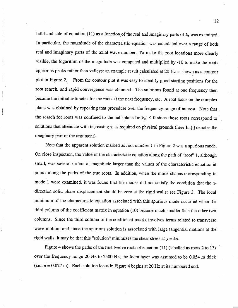
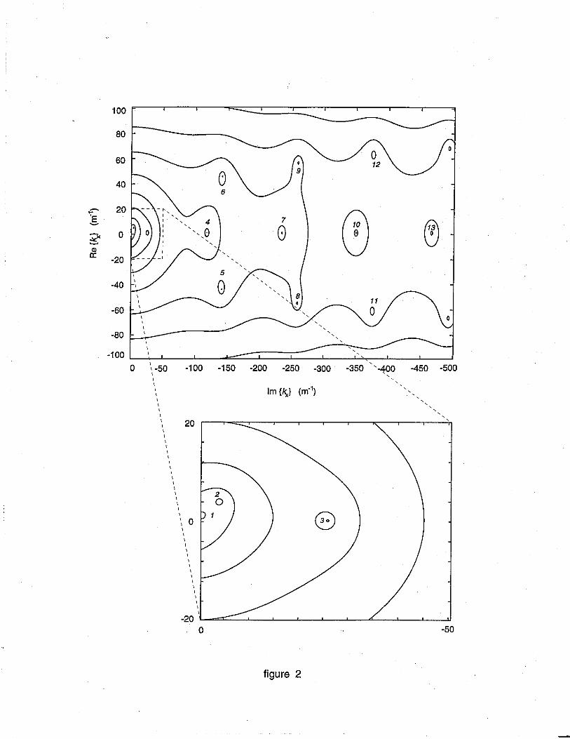
left-hand side of equation (11) as a function of the real and imaginary parts of kx was examined.

In particular, the magnitude of the characteristic equation was calculated over a range of both

real and imaginary parts of the axial wave number. To make the root locations more clearly

visible, the logarithm of the magnitude was computed and multiplied by -10 to make the roots

appear as peaks rather than valleys: an example result calculated at 20 Hz is shown as a contour

plot in Figure 2. From the contour plot it was easy to identify good starting positions for the

root search, and rapid convergence was obtained. The solutions found at one frequency then

became the initial estimates for the roots at the next frequency, etc. A root locus on the complex

plane was obtained by repeating that procedure over the frequency range of interest. Note that

the search for roots was confined to the half-plane Im[kxl s; 0 since those roots correspond to

solutions that attenuate with increasing x, as required on physical grounds (here Im[·] denotes the

imaginary part of the argument).

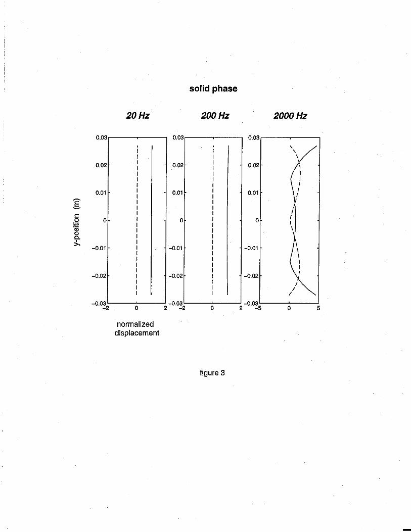
Note that the apparent solution marked as root number 1 in Figure 2 was a spurious mode.

On close inspection, the value of the characteristic equation along the path of "root" 1, although

small, was several orders of magnitude larger than the values of the characteristic equation at

points along the paths of the true roots. In addition, when the mode shapes corresponding to

mode 1 were examined, it was found that the modes did not satisfy the condition that the x­

direction solid phase displacement should be zero at the rigid walls: see Figure 3. The local

minimum of the characteristic equation associated with this spurious mode occurred when the

third column of the coefficient matrix in equation ( 10) became much smaller than the other two

columns. Since the third column of the coefficient matrix involves terms related to transverse

wave motion, and since the spurious solution is associated with large tangential motions at the

rigid walls, it may be that this "solution" minimizes the shear stress at y = ±d.

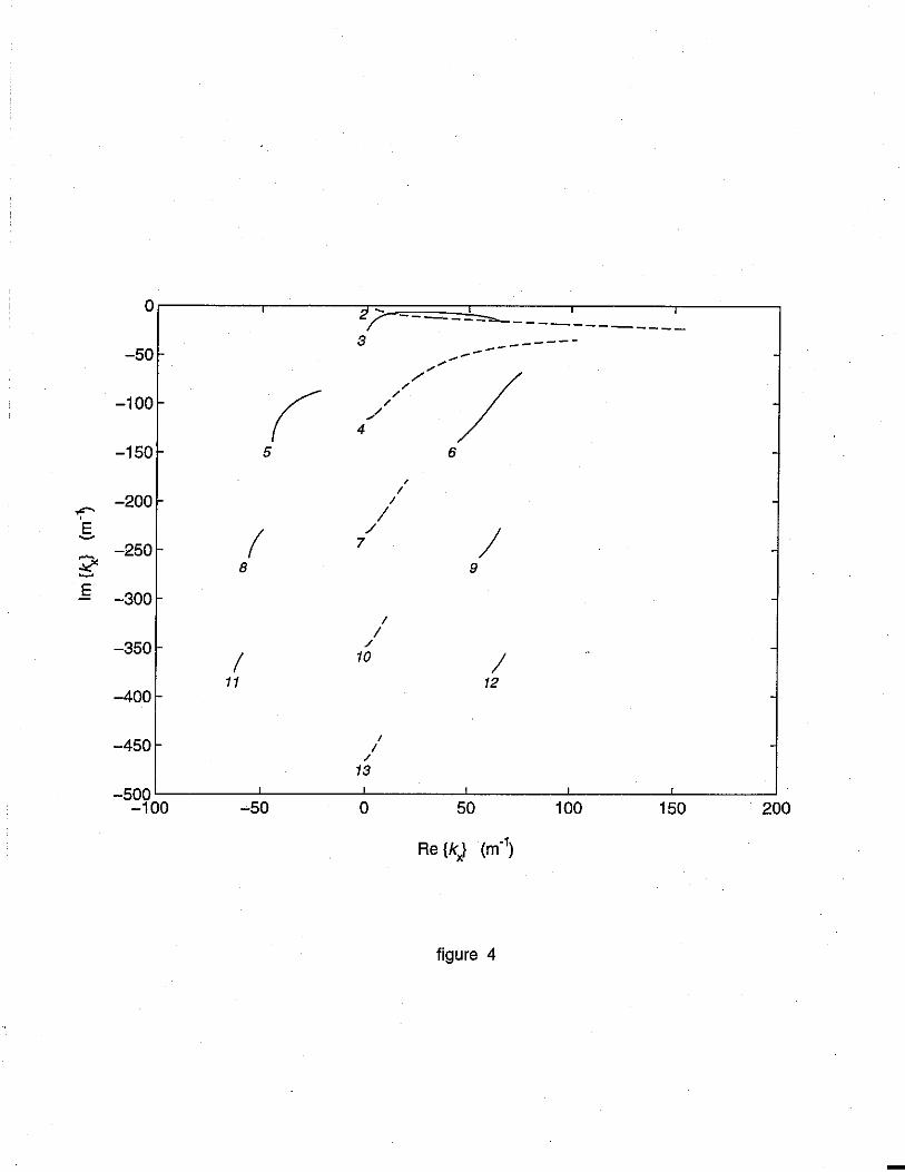
Figure 4 shows the paths of the first twelve roots of equation (11) (labelled as roots 2 to 13)

over the frequency range 20 Hz to 2500 Hz; the foam layer was assumed to be 0.054 m thick

(i.e., d = 0.027 m). Each solution locus in Figure 4 begins at 20 Hz at its numbered end.

13

The roots shown in Figure 4 can be separated into two groups: one associated with the fluid

phase (shown as dashed lines) and the other associated with the solid phase (shown as solid

lines). To determine the group to which a particular root belonged, two porous material sub­

models were derived by appropriately simplifying the complete model for the elastic porous

material. By assuming that there is no solid displacement (i.e., by assuming the frame of the

porous material to be rigid), the original governing equations for the foam can be reduced to the

equation governing wave motion in a rigid porous material. It will be recalled that only a single

longitudinal wave-type, i.e., the airborne wave, can propagate in the fluid phase of a rigid porous

material. To complement the rigid porous material model, a model for an elastic porous material

without interstitial fluid can be derived by deleting from the original governing equations all the

terms representing the effects of the fluid; in other words, the fluid pressure and density were

removed. As is to be expected for an elastic material, one longitudinal wave-type and one

transverse wave-type can propagate in this "empty" foam. Derivations of the characteristic

equations for the rigid and "empty" foam layers are presented in Appendices B and C,

respectively.

Figures 5 and 6 show the paths of the roots corresponding to the rigid and the "empty"

foam cases, respectively. From those two figures, one can easily classify a particular root of the

full solution as being primarily associated with motion of the solid or fluid phases of the foam.

Note that roots 5, 6, 8, 9, 11 and 12 do not originate on the imaginary kx axis: i.e., they are

complex in the low frequency limit. These complex roots appear in pairs in the third and fourth

quadrants of the kx plane, and in the low frequency limit the members of a pair (i.e., 5 and 6, 8

and 9, etc.) are approximately symmetrically placed with respect to the imaginary kx axis. Thus

the modes associated with roots 5, 8 and 11 have negative phase velocities (since Re[kxl < 0 for

these roots). Since Im[kxl is negative for each of these roots, the apparently negative x-travelling

modes amplify as they propagate. However, it was found that the group velocity (see Section

3.5) associated with each of the roots originating within. the third quadrant was positive: i.e., the

-

14

energy associated with each of these modes flows in the positive x-direction, away from the

air/foam interface, as is necessarily the case on physical grounds.

The interesting result that the phase and group velocities of certain modes have opposite

signs has been noted previously by Tolstoy and Usdin for the cases of both symmetric and

asymmetric mode propagation within plates in vacuo [25], by Crandall for wave propagation

along elastically supported Timoshenko beams [26,27], and by Fuller for flexural modes of fluid­

filled elastic shells [28,29].

Fuller also noted the appearance of complex roots in pairs, and further observed that since

the complex roots appeared in pairs symmetrically arrayed with respect to the imaginary kx axis,

each pair combines to form a stationary wave pattern whose amplitude decays away from

discontinuities (e.g., the air/foam interface in the present instance). In the present instance, the

spatial pattern associated with each of the complex root pairs is a purely decaying stationary

wave field only in the low frequency limit. Owing to the dissipation within the elastic porous

medium, a propagating component appears in combination with a stationary component as the

frequency increases. Finally it may be possible that the members of a pair of complex roots

could be combined to form a single composite mode, but that possibility has not been pursued

here.

3.5. MODAL PHASE VELOCITIES, GROUP VELOCITIES AND ATTENUATION

The axial phase velocity, Cph = rotp, and the group velocity [30]

c = dro = 2rcL g d/3 d/3 (22)

for modes 2 to 13 are shown in Figure 7, along with the attenuation per wavelength, a,').,, where p

= Re[kxl, a= Im[kx], A= 2rc/p, andf is the frequency in Hertz. The group velocities were

calculated from the root trajectories by numerical differentiation.

The phase velocities of the fluid-related modes are shown in Figure 7(a). The phase

velocity of mode 2 is essentially the same as the phase velocity of an airborne plane wave

travelling in an infinitely extended elastic porous medium: i.e., it is dispersive at low frequencies,

-

15

and approaches a constant value at high frequency ( of approximately 0.3co in the present

instance). The phase velocities of modes 4, 7, 10 and 13 are higher than that of mode 2.

However, note that the phase velocity of mode 4 drops towards that of mode 2 near 2000 Hz.

The latter is approximately the frequency at which the first symmetrical mode would cut on in a

hard walled duct filled with a medium having the sound speed of the fluid phase within the

elastic porous material (i.e., approximately 110 mis in the present case). It is likely that the

phase velocities of the other higher order modes would show the same behavior at sufficiently

high frequencies.

The phase velocities of the solid-related modes behave somewhat differently: see Figure

7(b). The phase velocity of mode 3 approaches a finite, low frequency limit and at higher·

frequencies drops to approximately that of the frame wave travelling in an infinitely extended

elastic porous medium (i.e., approximately 250 mis). The behavior of the phase velocity of

mode 3 changes from one type of behavior to another in the vicinity of 900 Hz. This is

approximately the "cut on" frequency that would be expected for the first cross-duct mode

involving primarily shearing motion of the solid phase (i.e., the frequency at which the duct

width is one-half a wavelength of the transverse wave). (Note that the phrase "cut on" is placed

in quotes here and in the following since in dissipative media of the type considered here there is

no clear distinction between propagating and non-propagating waves, and hence no unique cut on

frequency.) The phase velocities of the pairs of modes 5 and 6, 8 and 9, and 11 and 12, all

appear to approach zero as the frequency decreases. Because of the symmetry of the paired

roots, the phase velocities of modes 5 and 6 are approximately the same at low frequencies, while

they begin to diverge as the frequency increases. The same behavior is displayed by mode pairs

8 and 9, and 11 and 12.

The group velocities for the fluid-related modes are shown in Figure 7(c). The phase and

group velocities of mode 2 are almost identical, as would be expected for a plane wave, except in

the region in which there is significant dispersion: i.e., below 250 Hz. The group velocity of

mode 4 is larger than that of mode 2 in the low frequency limit, then drops below that of mode 2

-

16

in the vicinity of its "cut on" frequency; it then presumably approaches the mode 2 group

velocity from below. This behavior is consistent with the group velocities of higher order modes

propagating in a dissipative medium. It is expected that this behavior would be repeated at

progressively higher frequencies as each of the modes "cuts on" in sequence.

The group velocities of the solid-related modes are shown in Figure 7(d), where it can be

seen that the group velocity of mode 3 behaves differently than do the group velocities of the

paired modes. The group velocity of mode 3 very approximately follow the mode 3 phase

velocity. In contrast, the group velocities of the other modes decrease from large values as the

frequency is increased. It may prove that this apparently anomalous behavior is mitigated when

the mode pairs are considered as a single composite mode: that possibility should perhaps be the

subject of further investigation.

The attenuations per wavelength for the fluid-related modes are shown in Figure 7(e),

where it may be seen that the plane-wave-like mode 2 is by a substantial margin the least

attenuated mode, although the attenuation displayed by mode 4 is significantly reduced near its

"cut on" frequency. The latter behavior could be expected to repeat for each of the higher order

modes in tum at progressively higher frequencies.

The attenuations of the solid-related modes are shown in Figure 7(f). Here it may be seen

once again that the behavior of mode 3 differs from that of the other modes. Note also that the

attenuation per wavelength of mode 3 changes behavior in the vicinity of 900 Hz: i.e., near the

"cut on" of the shearing mode described above.

3.6. MODE SHAPES

The mode shapes associated with modes 2 to 13 are shown in Figure 8 for 20 Hz, 200 Hz

and 2000 Hz (note that at each frequency all solid and fluid axial and transverse displacements

are normalized by the magnitude of the axial solid displacement, hVnu I, at y = 0). First, it may XS

be seen that all of the modes satisfy the prescribed zero displacement boundary conditions at the

rigid walls, and that the axial displacement components are symmetric with respect to the plane y

= 0, while the transverse displacement components are anti-symmetric.

-

17

From Figure 8(c) it may be seen that mode 2 involves primarily fluid motion and is very

close to being a plane wave mode: i.e., its displacement is almost wholly axial and its phase is

nearly constant across the width of the duct. The mode does display progressively more

curvature as the frequency increases, however: see Figures 8(g) and 8(k).

Modes 4, 7, 10 and 13 are essentially higher order fluid modes. Mode 4 shows one spatial

period across the width of the duct, mode 7 shows two periods, etc., as would be expected for

symmetric modes: see Figures 8(c), 8(g) and 8(k). For all these modes, the magnitudes of the

axial and transverse fluid displacements are comparable. The solid motion associated with the

modes is relatively small compared with the fluid motion, though the relative significance of the

solid phase motion increases as the frequency increases. Finally, note that the solid motion

associated with these modes is primarily transverse (except for mode 13 at 20 Hz: see Figure

8(a)).

Mode 3 represents a primarily axial, uniformly-phased motion of the solid phase (i.e., the

solid is being sheared) and shows 1/2 a spatial period across the width of the duct. The

transverse motion of the solid phase does increase in significance as the frequency increases: see

Figures 8(a), 8(e) and 8(i). From Figures 8(c), 8(g) and 8(k) it may be seen that the fluid

displacement associated with mode 3 is comparable in magnitude to the solid motion,, and is

primarily axial. Note that at low frequencies, the fluid displacement is oppositely-phased at y =

±d and at y = 0, while the phase distribution is almost uniform at 2000 Hz ( compare Figures 8( d)

and 8(1)).

Modes 5 and 6, 8 and 9, and 11 and 12 are paired, as discussed above. It may be seen that

the magnitude of the displacement of each of the modes in one pair is the same, but that their

phase distributions differ. For all of these modes, the magnitudes of the axial and transverse

displacements are nearly the same. Note that the transverse displacement associated with mode 5

shows one spatial period across the duct width, that of mode 8 shows two spatial periods, and

that of mode 11 shows three spatial periods. At the same time there are 3/2 spatial periods of the

axial displacement across the width of the duct in the case of mode 5, 5/2 periods in the case of

-

18

mode 8, and 7 /2 periods in the case of mode 11. The behavior of both the axial and transverse

displacement is consistent with the requirements of symmetry in this geometry. The magnitudes

of the fluid and solid displacements are very similar for this family of modes, and the axial and

transverse displacement patterns within the fluid are essentially the same as those of the solid.

4. IMPEDANCE AND ABSORPTION OF A CONSTRAINED FOAM LA YER

4.1. INTRODUCTION

Once the allowed modes of propagation have been found, it is necessary to determine the

modal coefficients that accompany plane wave excitation of the foam's surface of the foam at x =

0. When the modal coefficients, i.e., the Atn's, have been determined, it is possible to calculate

the surface normal impedance of the foam. The techniques required to determine the surface

normal impedance are discussed in this section.

Recall that the foam layer is imagined to be of infinite depth, as shown in Figure 1. In

addition, a plane wave in the air is imagined to be normally incident on the surface of the porous

layer at x = 0. As has been indicated, the acoustical field variables in the foam and in the

reflected wave in the air can be separated into symmetric and asymmetric components. Since the

asymmetric modes have zero forcing under the excitation of a normally incident plane wave, we

can assume that the latter modes do not contribute to the forced solution. Therefore, solutions

can be found that consist solely of a superposition of symmetric modes.

4.2. SOUND FIELD IN THE REGION x s 0

The velocity potential for the sound field in the region x s O can be written as a

superposition of an incident plane wave and an infinite number of reflected modes that are each

symmetrical with respect to the x-axis, i.e., as

(23)

where: Btm is a modal coefficient, ko is the wave number in the incident fluid medium (i.e.,

ro/co), co is the speed of sound in the incident fluid medium and koxm = [(ro/co)2 - (mn/2d)2]112.

19

Note that in the region x !, 0 the sound pressure is related to the velocity potential by P =

Pod<Po/dt (where po is the ambient fluid density), the axial particle velocity, Vx, is equal to -

d<Po/dx, and the transverse fluid velocity, Vy, is equal to -d<Po/dy. The axial and transverse

particle displacements in the air space, uax and Uay, respectively, can then be determined from Vx

= jrouax and Vy= jrouay, respectively. Note that a harmonic time function, &(J)/, has been omitted

from equation (23).

4.3. OPEN SURFACE BOUNDARY CONDITIONS

"Open surface" boundary conditions are considered to apply at the air/foam interface: i.e.,

the porous material is considered to be unfaced. Boundary conditions of that type have been

described in References [9,15]. In summary, four boundary conditions must be satisfied at x = 0:

(i) -hp= s (ii) -(I-h)P=ax

(24a-d)

(iii) Vx = jro(l - h)ux + jrohUx (iv) 'txy = 0.

The first of equations (24) requires that the force per unit area acting on the fluid component of

the porous material be equal to the porosity times the pressure in the exterior acoustical field.

The second condition expresses a similar relation for the force acting on the solid phase. The

third equation requires the continuity of normal volume velocity at the surface. The final

condition indicates that there is no shear force acting on the free solid surface since the exterior

fluid is assumed to be inviscid.

4.4. APPLICATION OF THE BOUNDARY CONDITIONS

Upon evaluating the pressure from equation (23) and substituting that result together with

equation (19) into equation (24a), one obtains

-jrohp 0 ( 1 + L, B1m cos~]y) = m=0,2,4,

L, A1n[(Q+b1R)cos k1ynY + (Q+b2R)1 3ncos k2ynYJ. n In

(25)

20

To determine the modal coefficients in equation (25), i.e., the B1m's and the A1 11 's, it is

convenient to express the terms cosk1ynY and cosk2ynY as a series in cos(mn/2d)y: i.e.,

[(Q+b1R)cos k1ynY + (Q+b2R)~ 3ncos k2ynYl = L, Dqn cos~~y 1 n q=0,2,4.

where:

If" A qrc Dqn = d )(Q+b1R)cos k1ynY + (Q+b2R ) A~: cos k2ynY] cos 2dy dy

I f' A3 Don= 2d )(Q+b1R)cos k1ynY + (Q+b2R)A1:cos k2ynYl dy,

After collecting all the cosine terms, equation (25) can be rewritten as

L, UrohpoB1q + L, A1nDqn}cos~~Y = - jrohpo. q=o,2,4. n

q=2,4,6, · · ·

Similar manipulation of the next two boundary conditions, equations (24b) and (24c ), yields

L, Uro(I-h)poB1q + L, A1,,Eq11 }cos~~y = - jro{l-h)po q=0,2,4. n

In equations (30) and (31)

Eqn = _dif, [ (2Nk},, + A + Qb1) cos k1ynY + AA 3n (2Nk}n + A + Qb2) cos k2ynY k[ In ki

-d

qn OS ktynY] COS

2dy dy q = 2,4,6, · ..

fd

k 2 A k 2 Eon =

21d [ (2N__m__ + A + Qb1) cos k1ynY + A 3n (2N__m_ + A + Qb2) cos k2ynY

k[ In ki d

OS ktynY] dy

(26)

(27)

(28)

(29)

(30)

(31)

(32)

(33)

F -1..f d [ _ k (I-h+hb1) k _ k A 3n (I-h+hb2) qn - d 0) xn OS lynY 0) xnA kf In ki

·d

+ jro(I-h+hg)A6n ktyn cos krynY] cos qrcdy dy A1n k2 2

t

F, _ If d [ k (I-h+hbi) k k A3n (I-h+hb2) On - 2d - 0) xn OS lynY - 0) xnA-

k 2 In k2 I 2

.J

+ jro(I-h+hg)AA6n ktyn cos ktynY] dy In k 2

t

21

OS k2ynY

q = 2,4,6, - - . (34)

OS k2ynY

(35)

Since 'txy is anti-symmetric, it is expressed in terms of sink1ynY and sink2ynY, and it is .

convenient to expand the latter as a series in sin(mrc/2d)y before applying the last boundary

condition, equation (24d), which then becomes

(36)

where:

If d .kxnklyn . A3n kxnk2yn . Gqn = -d [ - 21,---sm k1ynY - 2;A sm k2ynY

kf In ki d

A6 k}n - ktn qrc + A n --~sin krynY] sin 2dy dy

In k2 t

q = 2,4,6, · · · (37)

When equation (29) is multiplied by cos(nc/2d)y and then integrated with respect toy from

-d to d, it can be transformed into an infinite set of linear equations: i.e.,

q = 0: jropohB10 + .L, AinDon = - jropoh n

q = 2 : jropohB12 + .L, A1nD2n = 0 n

q = 4: jropohB14 + .L, A1nD4n = 0 n (38)

q=6:

22

By taking advantage of the orthogonality of the sine and cosine functions, one can similarly

transform equations (30), (31) and (36) into three infinite sets of linear equations. These four

sets of equations can be truncated, arranged into a matrix equation as shown in Figure 9, and then

solved for the unknown modal coefficients.

4.5. SOLUTION FOR THE MODAL COEFFICIENTS

In general, for each mode allowed in the air space, it is necessary to allow three modes in

the porous layer in order to satisfy the four boundary conditions. That is, if one allows for four

acoustical modes in the exterior air space (i.e., q = 0,2,4,6), application of the four boundary

conditions at the air/foam interface results in sixteen equations which can be solved for sixteen

unknown modal coefficients: i.e., four modal coefficients in the air space, and twelve modal

coefficients in the porous layer.

The magnitudes of the modal coefficients determined by this procedure are shown in Figure

10. Note first that the magnitude of the last coefficient, A113, is anomalously large owing to a

truncation effect. This effect was observed to occur regardless of the number of modal

coefficients used. That is, when three modes were allowed in the air space and nine foam modes

were used, it was noted that modal coefficient A 11 o was anomalously large. When the

calculation was repeated using four modes in the air space and twelve modes in the foam, the

value of A110 was now calculated correctly, but A113 was too large. As a result, A113 was

considered to be inaccurate and was thus set to zero in the reconstructions described in section

4.6.

The fluid-related modal coefficients are shown in Figure IO(a), where it can be seen that

the plane-wave-like mode 2 is the most significant mode. The solid-related modal coefficients

are at least an order of magnitude smaller in magnitude than the fluid-related modal coefficients:

see Figure IO(b). In the air space, the plane wave modal coefficient, B10, is the largest

contributor, its magnitude tending towards unity in the low frequency limit: see Figure IO(c).

-

23

4.6. DISPLACEMENT FIELD RECONSTRUCTIONS

The modal coefficients can be inserted into equations (12) to (15), and (23) to reconstruct

the displacement fields within both the exterior air space and the foam. This operation was

performed at 20 Hz, 200 Hz and 2000 Hz both to visualize the displacement at the air/foam

interface (i.e., at x = 0), with the results shown in Figure 11, and to confirm that the volume

velocity boundary condition, equation (24c) was satisfied. (Note that boundary conditions (24a),

(24b) and (24d) were also directly verified, but those results are not presented here). At 20 Hz

and 200 Hz, the fluid displacement in the foam is almost plane and is nearly identical in

magnitude to that in the exterior air space (when the porosity weighting is taken into account: see

equation (24c) ). At 2000 Hz, the magnitude of the solid displacement is becoming large enough

to contribute visibly to the total result, and the fluid displacement is significantly non-planar,

even though the first higher order symmetrical mode does not cut on in the exterior air space

until approximately 3300 Hz.

4.7. MODAL CONTRIBUTIONS TO THE STRESS FIELDS

It was also of interest to quantify the contributions of the various modes to the stress fields

at the foam/air interface. Shown in Figure 12 are l'Vn I, l'Vn~x I and l'Vn, I as functions of mode ss v. s xya

number at 1000 Hz. The first two of these functions were evaluated at y = 0, while the latter was

evaluated at y = d (since 'txya is equal to zero at y = 0). These modal functions must be weighted

by their corresponding modal coefficients to determine the actual contribution of a particular

mode to a particular stress component. However, it can be concluded from Figures 12(b) and (c)

that the fluid-related modes (shaded columns) contribute very little to the stress within the solid

phase of the porous material. Figure 12(a), in contrast, shows that the solid-related modes can

make a significant contribution to the stress within the fluid phase of the porous material.

4.8. SURFACE NORMAL IMPEDANCE AND ABSORPTION

Strictly speaking, the normal specific acoustic impedance at the foam's surface (the ratio of

the pressure at the surface to the acoustic particle velocity into the surface) is a function of

position in the y-direction owing to the existence of the higher order modes in the regions x ~ 0

-

24

and x ;;:: 0. However, here it was of interest to calculate the plane wave surface normal

impedance that might be measured in a conventional standing wave tube apparatus [3,4]. In

standing wave tubes, measurements are usually made several tube-diameters from the sample

surface to minimize the effect of non-propagating higher order modes. In that case, the estimate

of the surface normal impedance is based on measurements of the incident and reflected plane

wave components only. The latter measurement can be simulated by estimating the foam's

surface impedance based on the incident and reflected plane waves in the region x :5 0: i.e.,

~ _ l+B10 iclx:o - 1 - B10

where Zc = poco, the characteristic impedance in the ambient medium.

(39)

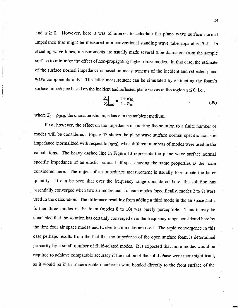
First, however, the effect on the impedance of limiting the solution to a finite number of

modes will be considered. Figure 13 shows the plane wave surface normal specific acoustic

impedance (normalized with respect to poco), when different numbers of modes were used in the

calculations. The heavy dashed line in Figure 13 represents the plane wave surface normal

specific impedance of an elastic porous half-space having the same properties as the foam

considered here. The object of an impedance measurement is usually to estimate the latter

quantity. It can be seen that over the frequency range considered here, the solution has

essentially converged when two air modes and six foam modes (specifically, modes 2 to 7) were

used in the calculation. The difference resulting from adding a third mode in the air space and a

further three modes in the foam (modes 8 to 10) was barely perceptible. Thus it may be

concluded that the solution has certainly converged over the frequency range considered here by

the time four air space modes and twelve foam modes are used. The rapid convergence in this

case perhaps results from the fact that the impedance of the open surface foam is determined

primarily by a small number of fluid-related modes. It is expected that more modes would be

required to achieve comparable accuracy if the motion of the solid phase were more significant,

as it would be if an impermeable membrane were bonded directly to the front surface of the

25

foam. Note finally that the impedance and absorption calculations shown here have been independently verified through finite element calculations: see Reference [31].

From Figure 13, it can be seen that the surface normal impedance in the constrained-edge case approaches that of a porous half-space at frequencies above approximately 1500 Hz for the material properties and geometry considered here. The feature appearing at approximately 900 Hz relates to the "cut on" of mode 3: i.e., the shearing mode of the solid. Below that frequency, the foam is stiffened by the effect of the edge constraints (i.e., the magnitude of the imaginary component of the surface impedance is increased with respect to that of the half-space). A further small discrepancy between the impedance of the constrained foam and of the porous half­space can be seen above 2000 Hz. This difference may result from the "cut on" of mode 4: i.e., the first higher order fluid-related mode.

The normal incidence absorption coefficient, <Xn = 1 - IB 1012, of the constrained-edge foam is shown in Figure 14. It can be seen that the absorption of the constrained foam layer is reduced compared to that of the porous half-space below the "cut on" of mode 3, but approaches the half-space value at higher frequencies after reaching a maximum of approximately 0.77 near 975 Hz.

4.9. EFFECT OF DUCT WIDTH

To illustrate the effect of duct width, calculations were also performed for an edge­constrained foam layer whose thickness was 0.027 m: i.e., d = 0.0135 m. Based on the convergence in the case of the 0.054 m foam layer, the calculation was performed using two air space modes and six foam modes. The axial wave numbers in this case are shown in Figure 15, and the surface normal impedance and absorption are shown in Figures 16 and 17, respectively. From Figure 16 it can be seen that the stiffening effect of the edge constraint extends to higher frequencies than in the case of the wider duct: i.e., the impedance feature that appeared near 900 Hz in the latter case now appears near 1800 Hz. This shift presumably relates to the delayed "cut on" of mode 3. The corresponding plot of the normal incidence absorption coefficient, Figure

26

17, is similar in character to that of Figure 14, except that the frequency of maximum absorption

has been shifted upwards by a factor of approximately 2.

It is of interest to be able to predict the frequency below which a foam sample is stiffened

by the effect of edge constraint. Below that frequency, the impedance of a constrained sample

may not accurately represent the impedance of the corresponding infinite sample. It has been

concluded here that the foam can be significantly stiffened at frequencies below the "cut on" of

the shearing mode in the solid, mode 3. At that frequency, the duct width is approximately one­

half a wavelength of the transverse wave in the elastic porous material. Thus in a rectangular

geometry, the frequency below which stiffening could be expected to be significant, fs, can be

calculated as

(40)

where c1 is the phase velocity of the transverse wave in the foam and 2d is the smallest cross­

dimension of the duct. In the present case.fs is 911 Hz and 1822 Hz for the 0.054 m and 0.027 m

width ducts, respectively. A different result would be expected to apply in a cylindrical

geometry, but equation (40) would offer general guidance when 2d is set equal to the tube

diameter.

Finally, note that the degree of stiffening due to the edge constraint will depend not just on

the stiffness of the foam, but also on the degree of coupling between the solid and the fluid

motions. That coupling is in turn determined by the fluid-acoustical parameters of the foam,

specifically the tortuosity (which quantifies the degree of inertial coupling between fluid and

solid) and the flow resistivity (which quantifies the degree of viscous coupling between fluid and

solid). Thus when the tortuosity of a foam is reduced towards unity (while holding the stiffness

of the solid phase constant), the stiffening effect of the edge constraint would be expected to

diminish: i.e., the stiffening effect will be much smaller in the case of a fully open cell foam than

for a partially reticulated foam of the type considered here. The stiffening effect would also be

expected to decrease if the flow resistivity were progressively reduced.

-

27

5. CONCLUSION

The main objective of the work presented here was to assess the effects of edge constraint

on the surface normal impedance of an elastic porous material when placed in a standing wave

tube. A modal solution procedure was developed that allows the boundary conditions at the

sample edges to be fully satisfied. Calculations for a simplified geometry that nonetheless

represents the salient features of a standing wave tube have shown that a constrained edge

stiffens the porous layer at low frequencies (at least when material parameters typical of

relatively stiff, partially reticulated polyurethane foams were used in the calculations). That

stiffening has a noticeable effect on both the surface normal impedance and the normal incidence

absorption coefficient of the constrained layer. Finally, a simple criterion, equation (40), was ·

developed to indicate whether the stiffening effect is likely to be of significance in a frequency

range of interest.

ACKNOWLEDGEMENT

The third author would like to dedicate this article to the memory of C.I. Holmer

-

28

6. REFERENCES

I. R.A. Scott 1946 Proceedings of the Physical Society 58, 253-264. An apparatus for accurate measurement of the acoustic impedance of sound-absorbing materials.

2. L.L. Beranek 1988 Acoustical Measurements. New York: American Institute of Physics.

3 A.F. Seybert and D.F. Ross 1977 Journal of the Acoustical Society of America 61, 1362-1370. Experimental determination of acoustic properties using a two-microphone random­excitation technique.

4. J.Y. Chung and D.A. Blaser 1980 Journal of the Acoustical Society of America 68, 907-921. Transfer function method of measuring in-duct acoustic properties. I. Theory. II. Experiment.

5. C. Zwikker and C.W. Kosten 1949 Sound Absorbing Materials. Amsterdam: Elsevier Press.

6. J.S. Bolton 1984 Ph.D. Thesis, Institute of Sound and Vibration Research, University of Southampton. Cepstral techniques in the measurement of acoustic reflection coefficients, with application to the determination of a~oustic properties of elastic porous materials.

7. J.S. Bolton and E.R. Green 1993 Applied Acoustics 39, 23-51. Normal incidence sound transmission through double-panel systems lined with relatively-stiff, partially reticulated, polyurethane foams.

8. J.S. Bolton and N.-M. Shiau 1989 Paper AIAA-89-1048 presented at the 12th AIAA Aeroacoustics Conference, San Antonio TX, Oct. 10-12, 1989. Random incidence transmission loss of lined, finite double panel systems.

9. N.-M. Shiau 1991 Ph.D. Thesis, School of Mechanical Engineering, Purdue University. Multi-dimensional wave propagation in elastic porous materials with applications to sound absorption, transmission and impedance measurement.

10. A. Cummings 1991 Journal of Sound and Vibration 151, 63-75. Impedance tube measurements on porous media: the effects of air-gaps around the sample.

11. R.A. Scott 1946 Proceedings of the Physical Society 58, 358-368. The propagation of sound between walls of porous material.

12. R.F. Lambert 1982 Journal of the Acoustical Society of America 73, 1139-1146. Surface acoustic admittance of highly porous open-cell foams.

13. M.A. Biot 1956 Journal of the Acoustical Society of America 28, 168-191. Theory of propagation of elastic waves in a fluid-saturated porous solid. I. Low-frequency range. II. Higher frequency range.

14. J.S. Bolton and N.-M. Shiau 1987 Paper AIAA-87-2660 presented at the 11th AIAA Aeroacoustics Conference, Sunnyvale CA, Oct. 19-21, 1987. Oblique incidence sound transmission through multi-panel structures lined with elastic porous material.

29

15. J.S. Bolton, N.-M. Shiau and Y.J. Kang 1996 Journal of Sound and Vibration.191, 317-347. Sound transmission through multi-panel structures lined with elastic porous materials.

16. K. Attenborough 1982 Physics Reports 82, 179-227. Acoustical characteristics of porous materials.

17. T. Pritz 1986 Journal of Sound and Vibration 106, 161-169. Frequency dependence of frame dynamic characteristics of mineral and glass wool materials.

18. M.E. Delany and E.N. Bazley 1969 National Physical Laboratory, Aerodynamics Division Report AC 37. Acoustical characteristics of fibrous absorbent materials.

19. M. Redwood 1960 Mechanical Waveguides. New York: Pergamon Press.

20. J. Miklowitz 1984 Elastic Waves and Waveguides. New York: North-Holland.

21. R. Lakes 1987 Paper appearing in the Proceedings of the 20th Midwestern Mechanics Conference, Purdue University, School of Mechanical Engineering, West Lafayette IN, August 31 - September 2, 1987. Foam materials with negative Poisson's ratios.

22. C. Bruer and J.S. Bolton 1987 Paper AIAA-87-2661 presented at the AIAA 11th Aeroacoustics Conference, Sunnyvale CA, Oct. 19-21, 1987. Vibro-acoustic damping of extended vibrating systems.

23. U. Ingard, F. Kirschner, J. Koch and M. Poldino 1989 Proceedings of INTER-NOISE 89, 1057-1062. Sound absorption by porous, flexible materials.

24. U. Ingard, F. Kirschner, J. Koch and M. Poldino 1990 Proceedings of INTER-NOISE 90, 225-230. Further studies of sound absorption by porous, flexible materials.

25. I. Tolstoy and E. Usdin 1957 Journal of the Acoustical Society of America 29, 37-42. Wave propagation in elastic plates: low and high mode dispersion.

26. S.H. Crandall 1957 Journal of Applied Mechanics 24, 622-623. Negative group velocities in continuous structures.

27. S.H. Crandall 1956 Proceedings of the Third Midwestern Conference on Solid Mechanics (Ann Arbor MI, April 1-2, 1956), 146-159. The Timoshenko beam on an elastic foundation.

28. C.R. Fuller 1981 Journal of Sound and Vibration 15, 207-228. The effects of wall discontinuities on the propagation of flexural waves in cylindrical shells.

29. C.R. Fuller 1982 Journal of Sound and Vibration 81, 501-518. Characteristics of wave propagation and energy distributions in cylindrical elastic shells filled with fluid.

30. L.E. Kinsler, A.R. Frey, A.B. Coppens and J.V. Sanders 1980 Fundamental of Acoustics. New York: John Wiley & Sons.

31. Y.J. Kang and J.S. Bolton 1995 Journal of the Acoustical Society of America 98, 635-643. Finite element modeling of isotropic elastic porous materials coupled with acoustical finite elements. ·

-

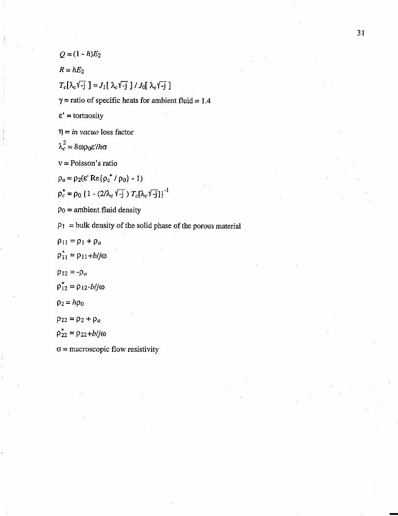
Appendix A: Parameters and Formulae for Calculations Related to Elastic Porous

Materials.

30

The parameters and formulae required to perform the calculations presented in this paper

are listed in this Appendix. The notation used here is the same as that employed previously by

the authors [9,14,15] and is largely based on Biot's nomenclature [13].

a1 = (Pi1R - PizQ)/(p;zQ-pjzR)

2 2 * * a2 = (PR - Q )/[ro (P22Q - P12R)]

A= vE1 /(1 + V)(l - 2v)

A1 = ro2(pi1 R - 2pj2 Q + p;2 P) I (PR- Q2)

A2 = ro4[pj1 P22 - (Pi2)2] /(PR - Q2)

b=-rop0 E' hlm{p/ /po}

b1 = a1 - Oz kf

b2 = a1 - az k?

co = speed of sound in ambient fluid = 340 mis

Em= static bulk Young's modulus (real)

Eo= poco2

E1 = Em(l + ftl), in vacuo bulk dynamic Young's modulus

E2 = Eo { 1 + [2(y-1)/N// Ac '1-j] Tc[NJ~ Ac '1-j] )-1

g = -Pi2 I P22

h = porosity

Jo, Ji = Bessel functions of the first kind, zero and first order, respectively

k? = (ro2/N)[Pi°1 - (P;2)2IP;2l

k{,2 =(A1±-YA{-4A2 )/2

N = E1 I 2(1 + v), in vacuo bulk shear modulus

Npr = Prandtl number for ambient fluid= 0.732

P=A +2N

Q = (l - h)E2

R=hE2

Tc[Ac\'-.f] =l1[ Ac\'-.J] I Jo[ Ac\'-.J]

y = ratio of specific heats for ambient fluid = 1.4

e' = tortuosity

11 = in vacuo loss factor 2

Ac = 8ropoE'/hcr

v = Poisson's ratio

Pa= P2(E' Re{p/ I Po) - 1)

p; = Po { 1 - (2/A.c \'-.J) Tc[A-c \'-.J]) "1

Po = ambient fluid density

P 1 = bulk density of the solid phase of the porous material

P11 =PI+ Pa

Pi1 = P11+b/jro

P12 = -Pa

Pi2 = P12-b/jro

P2 = hpo

P22 = P2+ Pa

P;2 = P22 +bljro

cr = macroscopic flow resistivity

31

-

32

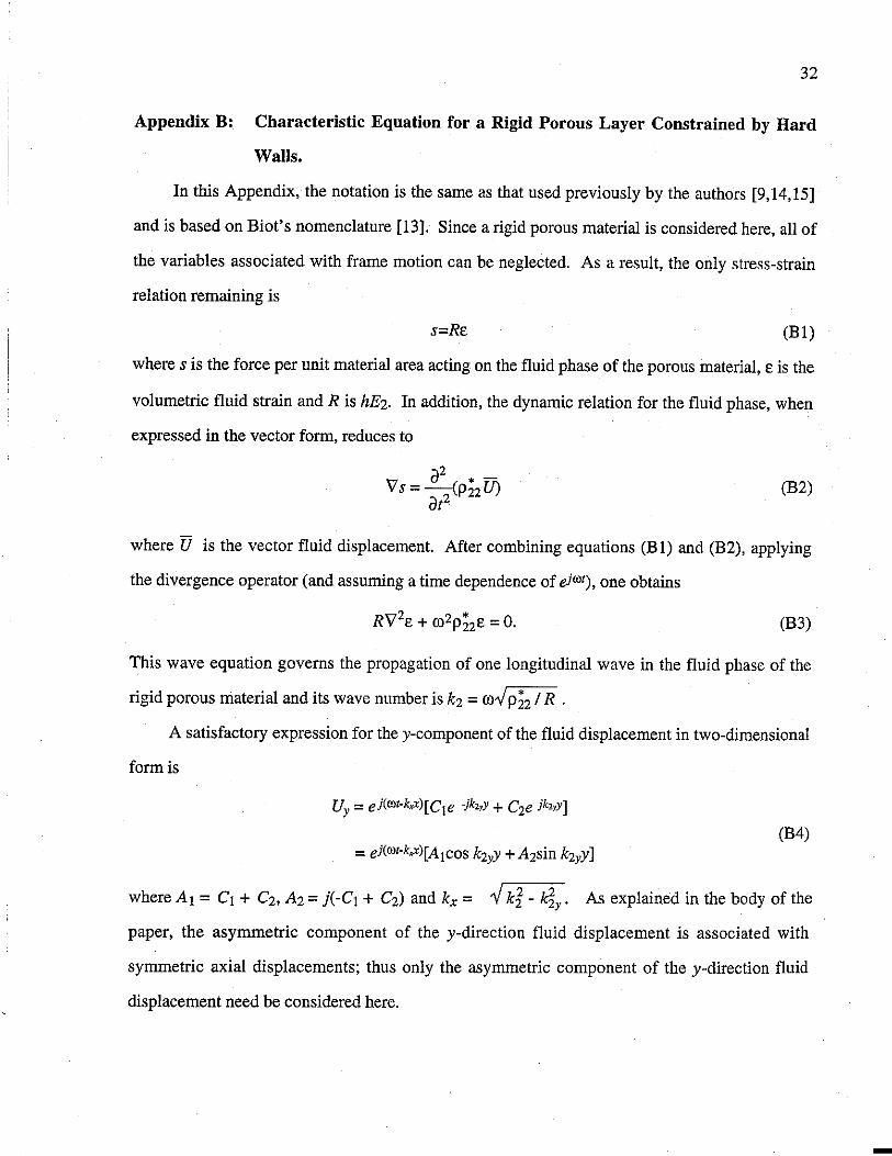
Appendix B: Characteristic Equation for a Rigid Porous Layer Constrained by Hard

Walls.

In this Appendix, the notation is the same as that used previously by the authors [9,14,15]

and is based on Biot's nomenclature [13]. Since a rigid porous material is considered here, all of

the variables associated with frame motion can be neglected. As a result, the only stress-strain

relation remaining is

s=Re (Bl)

where s is the force per unit material area acting on the fluid phase of the porous material, e is the

volumetric fluid strain and R is hE2. In addition, the dynamic relation for the fluid phase, when

expressed in the vector form, reduces to

az * -v' s = --=-:-(pzz U)

dt2 (B2)

where U is the vector fluid displacement. After combining equations (B 1) and (B2), applying

the divergence operator (and assuming a time dependence of ej<JJt), one obtains

(B3)

This wave equation governs the propagation of one longitudinal wave in the fluid phase of the

rigid porous material and its wave number is k2 = w,/ p;2 / R .

A satisfactory expression for the y-component of the fluid displacement in two-dimensional

form is

(B4) = ej(rot-k.x)[A1cos k2yY +A2sin k2yY]

where A1 = C1 + C2, A2 = j(-C1 + C2) and kx = -V k:j; - k~y. As explained in the body of the

paper, the asymmetric component of the y-direction fluid displacement is associated with

symmetric axial displacements; thus only the asymmetric component of the y-direction fluid

displacement need be considered here.

-

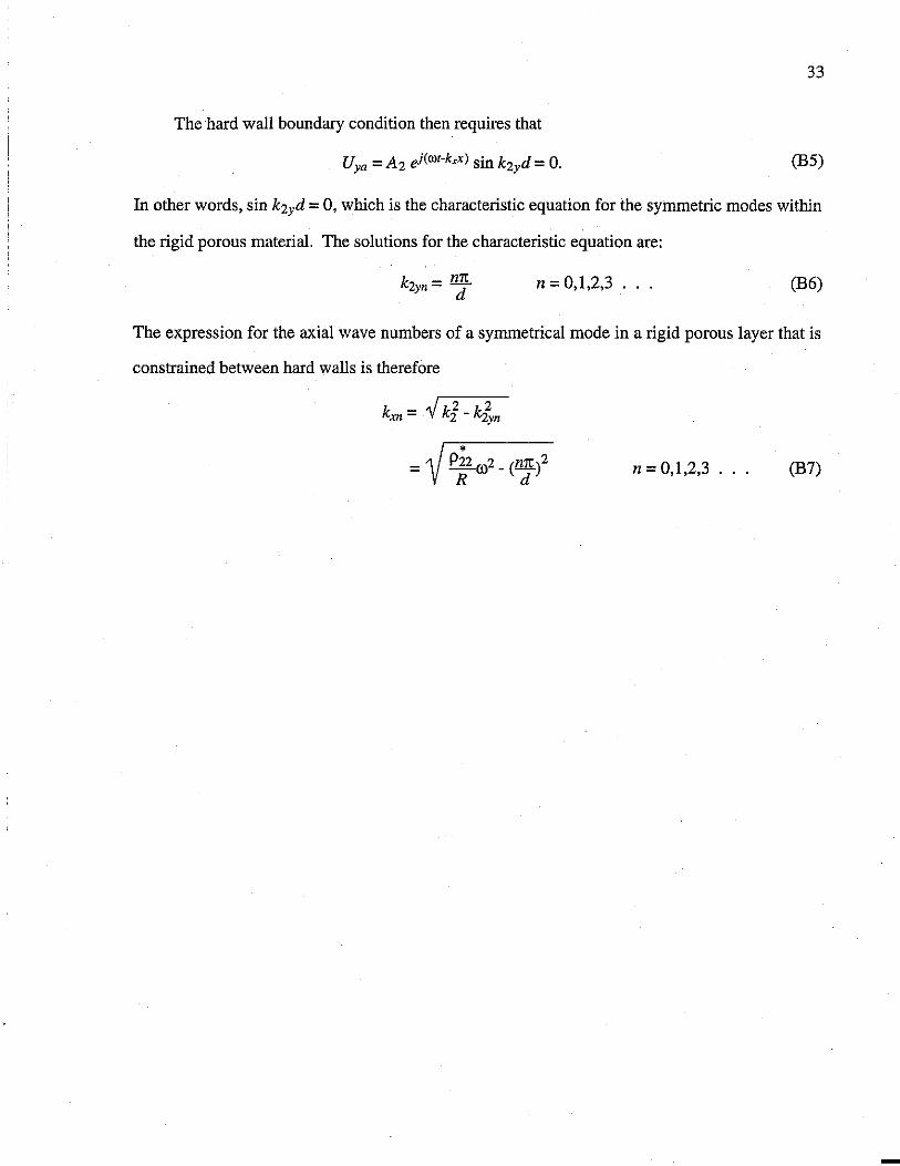
The hard wall boundary condition then requires that

Uya = A2 ej(rot-k.x) sin k2yd = 0.

33

(BS)

In other words, sin k2yd = 0, which is the characteristic equation for the symmetric modes within

the rigid porous material. The solutions for the characteristic equation are:

k2 - mt yn- d n=0,1,2,3 ... (B6)

The expression for the axial wave numbers of a symmetrical mode in a rigid porous layer that is

constrained between hard walls is therefore

kxn = -./ k'j; - k{yn

= ~ f P;2 002 _ (nrr,)2 V R d

n = 0,1,2,3 ... (B7)

-

34

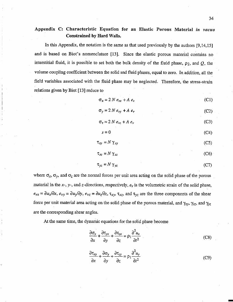
Appendix C: Characteristic Equation for an Elastic Porous Material in vacuo

Constrained by Hard Walls.

In this Appendix, the notation is the same as that used previously by the authors [9,14,15]

and is based on Biot's nomenclature [13]. Since the elastic porous material contains no

interstitial fluid, it is possible to set both the bulk density of the fluid phase, pz, and Q, the

volume coupling coefficient between the solid and fluid phases, equal to zero. In addition, all the

field variables associated with the fluid phase may be neglected. Therefore, the stress-strain

relations given by Biot [13] reduce to

CTx=2Nevx+Aev

cry=2Nevy+Aev

cr, = 2 N ev, + A ev

s=O

'txz =NYxz

(Cl)

(CZ) .

(C3)

(C4)

(CS)

(C6)

(C7)

where crx, cry, and CTz are the normal forces per unit area acting on the solid phase of the porous

material in the x-, y-, and z-directions, respectively, ev is the volumetric strain of the solid phase,

evx = duxlrJx, evy = du/rJy, evz = duzldz, 'txy, 'txz, and 'tyz are the three components of the shear

force per unit material area acting on the solid phase of the porous material, and 'Yxy, 'Yxz, and 'Yyz

are the corresponding shear angles.

At the same time, the dynamic equations for the solid phase become

2 dcr x d'tyx d'tzx d Ux -+--+--=p1--dx dy dz dt2

2 d'txy day d'tzy _ d Uy --+-+---P1--dx dy dz dt2

(CS)

(C9)

-

35

(ClO)

Equations (Cl) to (ClO) can be manipulated to yield a single vector equation

(Cll)

where u is the vector displacement of the solid component of the porous· material and a time

dependence of ejrot has been assumed. By applying the divergence operator to equation (Cl 1),

one obtains

(C12)

which is the wave equation governing the propagation of a single longitudinal wave in the

evacuated porous material. Application of the curl operator to equation (Cl 1) results in

(Cl3)

which is the wave equation governing the propagation of rotational strains in the evacuated

porous material. In equation (Cl3), co is the vector rotational displacement of the solid phase of

the porous material.

Thus, one longitudinal wave as well as one transverse wave can propagate in an evacuated

porous material; their wave numbers are, respectively,

(Cl4)

(Cl5)

Satisfactory expressions for the solutions of the two-dimensional versions of wave

equations (Cl2) and (C13) take the form

(Cl6)

(C17)

-

36

where Wz is the z-component of the rotational strain, k1y = V k? - k} and k,y = V k( - k} . The

solid displacements in the x- and y-directions then become

(C18)

(Cl9)

The complex coefficients, D1 to Ds, can be expressed in terms of C1 to C4 and the various wave

numbers [9,13,14], and consequently, equations (Cl8) and (Cl9) can be rewritten as

(C20)

(C21) .

By replacing the exponential terms with trigonometric functions, the solid displacements

can be separated into components that are symmetric and asymmetric with respect to the plane

y = 0. The symmetric components are:

(C22)

(C23)

components are

(C24)

(C25)

Since only the symmetric modes are considered here, the hard wall boundary condition is

applied at y = d to the symmetric component of axial solid displacement, Uxs, and the asymmetric

-

37

component of transverse solid displacement, Uya· The resulting equations can then be arranged in

matrix form: i.e.,

~osk1yd kt

kiy sin k1yd kt

kx . k d - -sm ry k2

t

[~:] =[~]. (C26)

By setting the determinant of the coefficient matrix to zero, the characteristic equation can be

obtained:

(C27)

The latter equation can be solved for the kxn's as described in the body of the paper.

-

FIGURE LEGENDS

Figure 1. Coordinate system for constrained foam layer bounded by hard walls.

Figure 2. Contour plot at 20 Hz of -10 times the logarithm to the base ten of the sum of the

magnitude of the left-hand side of the characteristic equation for the symmetric

modes (equation (11)) plotted versus the real and imaginary parts of the axial wave

number, kx- The numbers on the figure denote peak locations.

Figure 3. Plot of I\Jfiuxsl (solid line) and I\Jfluyal (dashed line) at 20 Hz, 200 Hz and 2000 Hz.

Note that the plotted results are normalized by the value of I\Jfluxsl at y = 0.

Figure 4. Axial wave numbers for 0.054 m thick, constr.ained foam layer bonded to hard

surfaces at y = ±0.027 m. The roots are denoted by numbers corresponding to the

peak locations shown in Figure 2. Dashed lines show fluid-related roots, while solid

lines show solid-related roots. All roots are plotted over the frequency range 20 Hz

(at the numbered end) to 2500 Hz.

Figure 5. Axial wave numbers for the foam with rigid frame. All wave numbers are plotted

over the frequency range 20 Hz to 2500 Hz. The roots are marked at 20 Hz, 500 Hz,

1000 Hz, 1500 Hz, 2000 Hz and 2500 Hz.

Figure 6. Axial wave numbers for the foam without interstitial fluid. All wave numbers are

plotted over the frequency range 20 Hz to 2500 Hz. The roots are marked at 20 Hz,

500 Hz, 1000 Hz, 1500 Hz, 2000 Hz and 2500 Hz.

Figure 7. Axial modal phase velocities, group velocities, and attenuation per wavelength. The

phase and group velocities are normalized by the speed of sound in air, co. (a) Axial

phase velocities of fluid-related modes; (b) axial phase velocities of solid-related

modes; (c) axial group velocities of fluid-related modes; (d) axial group velocities of

solid-related modes; (e) attenuation per wavelength of fluid-related modes; (f)

attenuation per wavelength of solid-related modes.

Figure 8. Plots of modal displacement magnitude and phase. At each frequency, all solid and

fluid axial and transverse displacements are normalized by the magnitude of the axial

solid displacement, l'lfnu I at y = 0. Axial displacement magnitudes and phases are XS

shown as solid lines; transverse displacement magnitudes and phases are shown as

dashed lines. (a) l'lfnu I and l'lfnu I at 20 Hz. (b) Phases of 'lfn and 'lfnu at 20 Hz. xs ya uxs ya

(c) 1\lfnu I and l'lfnu I at 20 Hz. (d) Phases of'lfnu and 'lfnu at 20 Hz. (e) I\Jfn I XS ya XS ya Uxs

and l'lfnu I at 200 Hz. (f) Phases of 'lfn and. 'lfnu at 200 Hz. (g) l'lfnu I and ya Uxs ya xs

l\lfnu I at 200 Hz. (h) Phases of 'lfnu and 'lfnu at 200 Hz. (i) l'lfnu I and l'lfn I at ya XS ya XS Uya

2000 Hz. G) Phases of 'lfnu and 'lfnu at 2000 Hz. (k) l'lfnu I and l'lfnu I at 2000 XS ya XS ya

Hz. (1) Phases of '!'nu and 'lfnu at 2000 Hz. XS ya

Figure 9. Matrix equation for modal coefficients.

Figure 10. Magnitude of modal coefficients. (a) Fluid-related modes in foam. (b) Solid-related

modes in foam. ( c) reflected modes in exterior air space.

Figure 11. Axial and transverse displacements of solid and fluid phases in the foam and in the

exterior air space at x = 0 at 20 Hz, 200 Hz and 2000 Hz. Axial displacements are

shown as solid lines, and transverse displacements as dashed lines. Calculations are

for unit amplitude incident plane wave (see equation (23)). (a) Magnitudes and (b)

phases of Ux5 and Uya (labelled as "solid"), Ux5

and Uya (labelled as "fluid"), and Uax:,

and Uay (labelled as "air").

Figure 12. (a) I\Jfn I at y = 0, (b) l'lfna I at y = 0, and (c) l\lfn- I at y = d, all evaluated at 1000 Ss XS ,r~xya

Hz. Shaded columns denote fluid-related modes, and plain columns denote solid-

related modes.

Figure 13. Normalized plane wave surface normal specific acoustic impedance of constrained

foam layer (2d = 0.054 m).

Figure 14. Normal absorption coefficient for constrained foam layer (2d = 0.054 m).

Figure 15. Axial wave numbers for 0.027 m thick constrained foam layer. Dashed lines show

fluid-related roots while solid lines show solid-related roots. All roots are plotted

over the frequency range 20 Hz to 2500 Hz.

Figure 16. Normalized .plane wave surface normal specific acoustic impedance of constrained

foam layer (2d = 0.027 m).

Figure 17. Normal absorption coefficient for constrained foam layer (2d = 0.027 m).

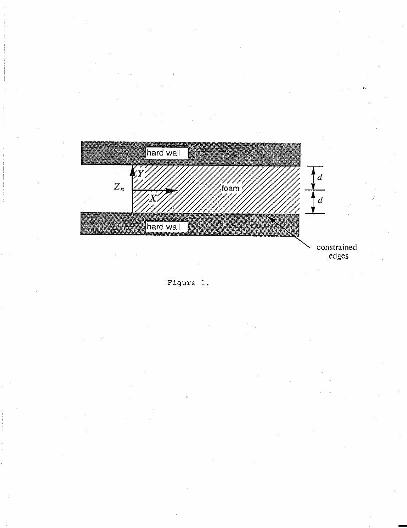
Figure 1.

d

d

constrained edges

-

100

80

60

40

- 20 i :Q< 0 -" a: -20

-40

' ' -60 ' ' ' -80 '

-100

0 \ -50 ' ' ' ' ' ' '

' ' '

' 4 ' ',,0

-100

20

', 0 ' '

' ' ' '

-20

' ' ' '

0

'

0 6

'

5

0

-150

2 0

0 0

' 12 9

0 7

~ 0 .

' '

11

0 ' ' 0 ' ' ' ' '

-200 -250 -300 -350 '-4~0 -450 -500

'

Im {'sc} (m"') ' '

' '

-50

figure 2

solid phase

20Hz 200Hz 2000Hz

0.03 0.03 0.03

' \ I \ I \

0.02 0.02 I 0.02 I I I I I I I I

0.01 0.01 I 0.01 I I I

~

I E ~ I

I I C: I 0 0 0 I 0 I E I U) I I 0 I 0. >, I I -0.01 -0.01 I -0.01 I I I I I I I I I -0.02 -0.02 I -0.02

I I I I I I

-0.03 -0.03 -0.03 -2 0 2 -2 0 2 -5 0 5

normalized displacement

figure 3

-

0 ' 2~ ___________ :__

3 --------50 ---- ----/

/ /

-100- ( /

/ -__ ,, 4

-150 >- 5 6 -,

I -200 >- I

~ I E

( /

/ ~

7

~ -250 >-

8 9 -E -300- -I

I -350- / -

I 10 / 11 12

-400- -

-450 I I -

/

13

-500 ' ' ' ' ' -100 -50 0 50 100 150 200

Re {k) (m-1)

figure 4

-

0 ' • ~----t- I I I

-------+----+----+ -so~ --+-------+ . ,, ,,

.,¥

-100~ I'

"' . +¥'

-150- .

l ~ -200- -f . - / 'E ~ - -250 . .)C -E

-300

-350~ I .

-400~ .

-450~ I .

-500 ' ' ' ' '

-100 -50 0 50 100 150 200

Re{k) (m-1)

figure 5

-

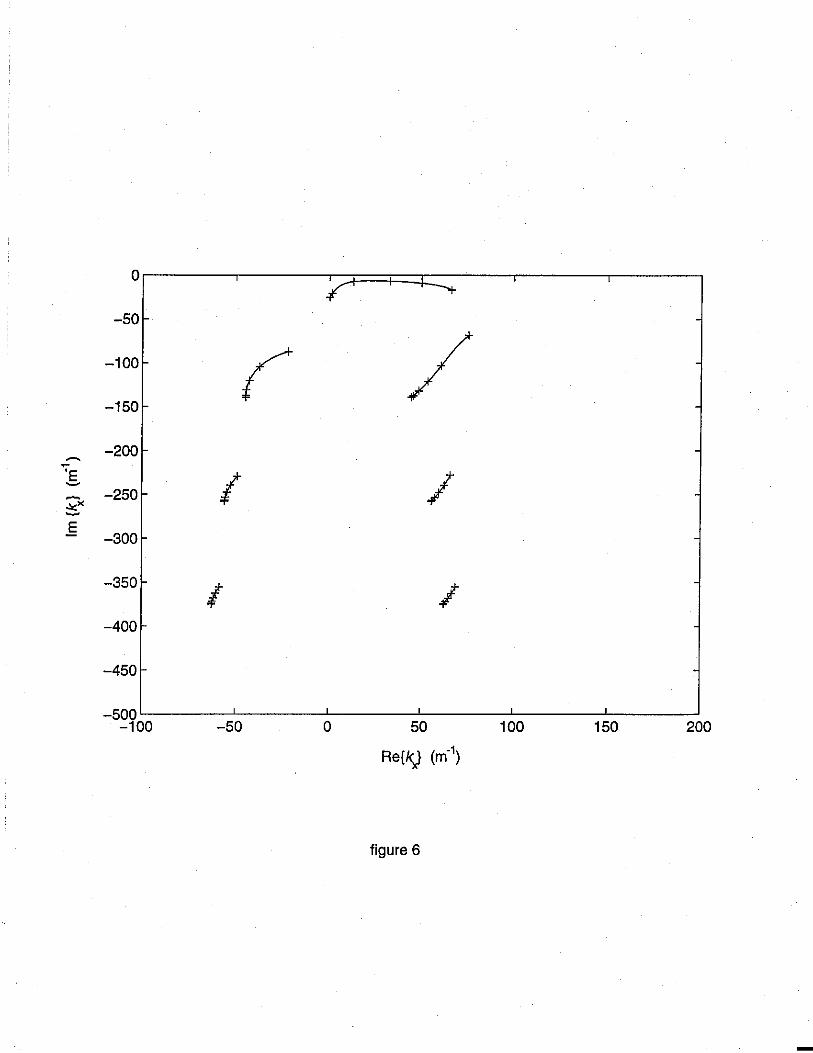
0 ' ' .

-50>- -

-100>- / -

-150>-

-200- -~

o;-E

I I ~ - -250- --"'" -E

-300- -

-350 >-

I I -

-400 >-

-450 >- .

-500 ' ' ' ' -100 -50 0 50 100 150 200

Re{k) (m-1)

figure 6

-

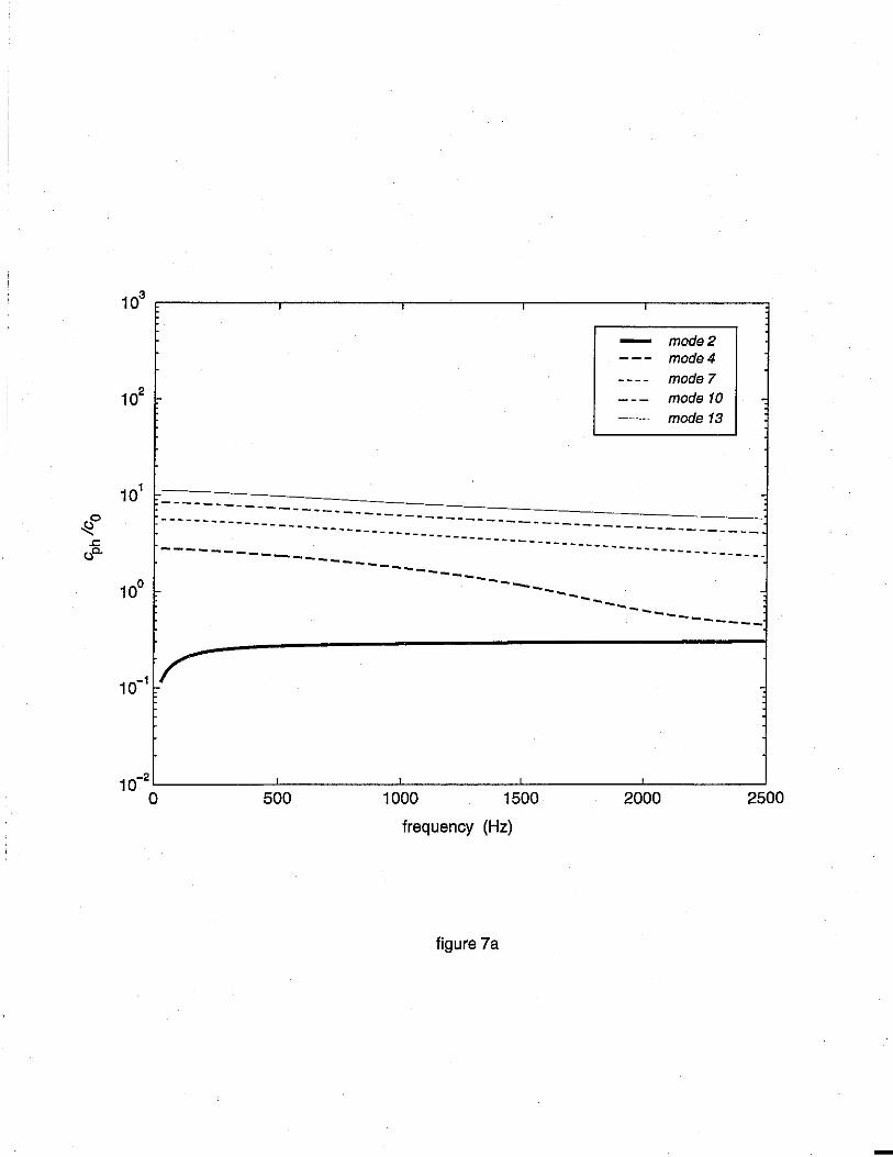
103 ,--------,---------,---------,------~-----~

' ' ' '

' '

mode2 mode4

moda7 mode 10 mode 13

.

.

.

101 r~:-~:=:=_~-=~-~:=:=_~-===-=-=-=--:-=-=-=-==::-::::-::~----------J· --------------------------------------------------------·

--------- ------- --------- ---------------------------------

10° - .

.

.

10-2 '-------''--------''-------~·-------'·~-------' 0 500 1000 1500 2000 2500

frequency (Hz)

figure 7a

-

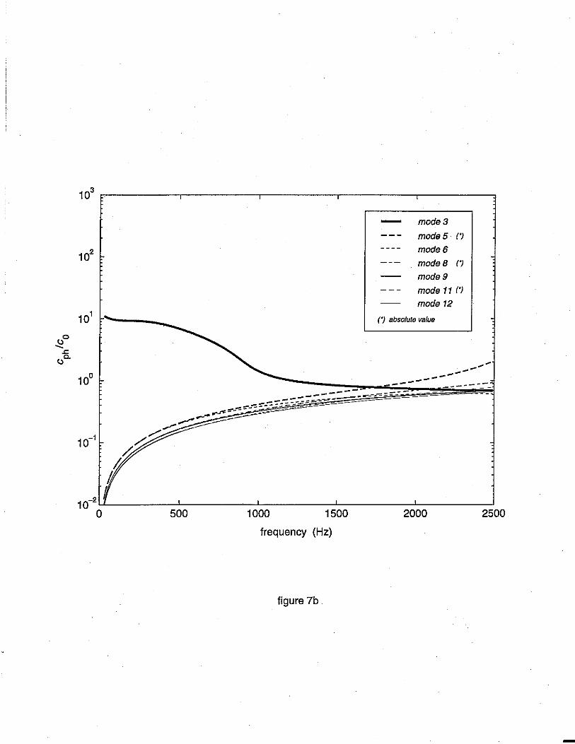
mode3

mode 5 ('/

mode6

modeB ('/

mode9

mode 11 ('/

mode 12

('/ absolute value

10-2L.L...------'-------'-------'-------'-------' 0 500 1000 1500 2000 2500

frequency (Hz)

figure 7b

-

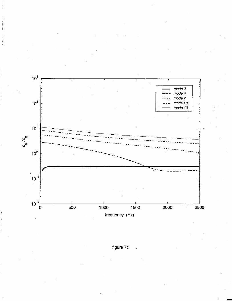
103 ' ' . .

' mode2 mode4

.

. model

102 ~ mode 10 mode 13

101 r-~-:-~-":-~--~-~=:-~-~--~=========-----___ J--------- ------------ --- -------- - --------- ----------- ---------- ------ --- -- -------- ---- --- --- --- ---= 10° -

-----------------------------~ ',, ' ------------------------.:-:::----------1 I/ --,_ ,. -------------.

.

.

10-2~------~·-------~·------~·-------~·------~

0 500 1000 1500 2000 2500

frequency (Hz)

figure 7c

-

' ' ' ' ' ' ' ' ' ' ' ' ' ,_ -- ------ --- --

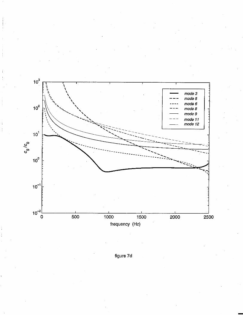
mode3 mode5 mode6 modeB mode9

mode 11 mode 12

----------- ......... , --------- ......... -------- ......... ----------=-.!"!,,~ ~,- .. ---.... , ...... -- ---

10-2L--------'-------'-------'-------'---'--------' 0 500 1000 1500 2000 2500

frequency (Hz)

figure 7d

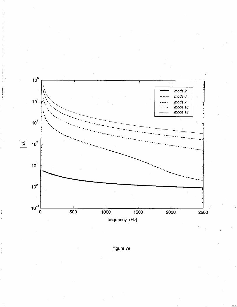
I \ \

' ' ' ',, ....... -- ---

mode2 mode4

model mode 10 mode 13

-... ----..... ------ -~=~~=-:=-~~~----_______ J ........ .......... ........ ........ .... _ ------------...... _

........ ........ ........ ........ ........ ........ ------

--.. ----- ....... _ --------------- ...... _ ------------ ------- -------- ---- ---- --- --- --- ---- ----

10-1 L--------'-------'-------'---------'--------' 0 500 1000 1500 2000 2500

frequency (Hz)

figure 7e

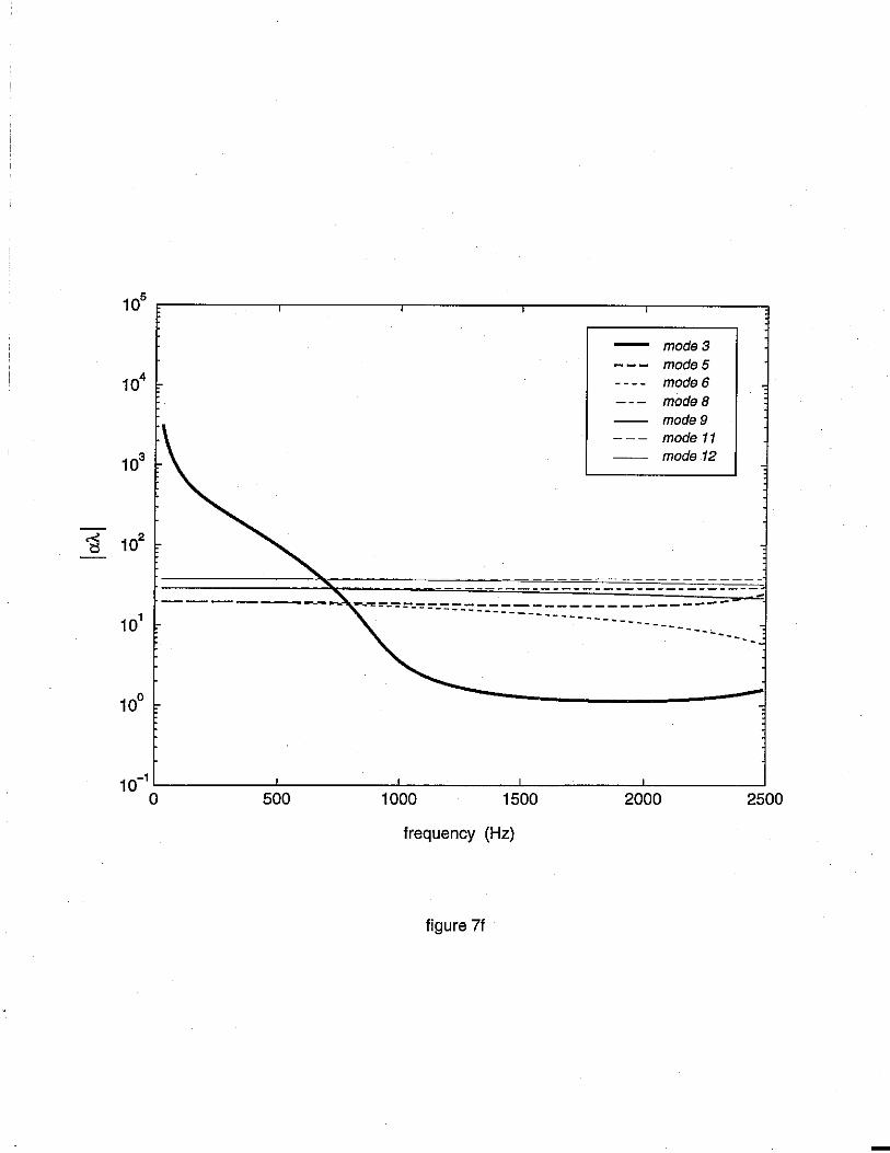
105

- mode3 mode5

104 mode6 mode8 mode9 mode 11

103 mode 12

-------------------------------------- - --- -=----==--- - -- --- -- - --- - - - -------- ------- ----- ---- -- ---- --- ---

10-1 ~-----~-----~-----~-----~-----~

0 500 1000 1500 2000 2500

frequency (Hz)

figure 71

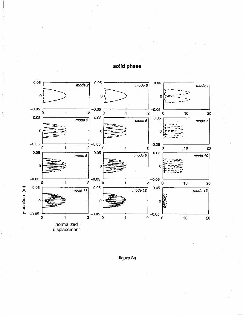
I I

solid phase

0.05 mode2

0.05 mode3

0.05 mode4

)------.., 0 0 0 7------------ ..

12- - ------0.05 -0.05 -0.05

0 1 2 0 2 0 10 20 0.05

mode5 0.05 mode6

0.05 mode7 -- ·=- ---=- 1--- - - - -

- - :. ;.:.~~~-= 0 i- - - oi--=:: ~ 0 - - ; )..,__-:_ :_ ---_.,, -~- -- ·=- ~-=--=-=---0.05 -0.05 -0.05

0 2 0 2 0 10 20 0.05

modeB 0.05

mode9 0.05

mode 10

-- - . -- - . ~f 0 -- - 0 ---- 0 . ~ "" . ~ _,

-b.05 -0.05 -0.05 0 1 2 0 1 2 0 10 20

~ 0.05 0.05 0.05 E mode 11 mode 12 mode 13 ~

C ~ , 0 0 0 0 :;:.

~ 'iii 0 C

Cl. ' >, -0.05 -0.05 -0.05

0 1 2 0 2 0 10 20

normalized displacement

figure Ba

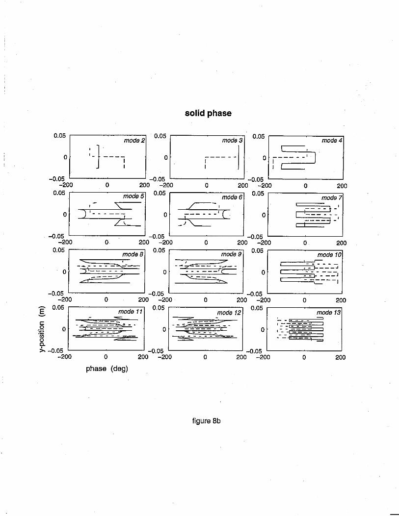
solid phase

0.05 ~-------~ mode2

0·05 ------m-o-de_3_ 0·05 ~------m-o-de_4_

0 :-}---7 0 of-~ -0.05 L.._ _______ _J -0.05 ~------- -0.05 '----------'

-200 0 200 -200 0 200 -200 0 200 o.o5 mode 5 o.o5 ~-----m-o-de_6_ o.o5 ~------m-o-de-7

0 ) :- - - -.,_)~, - 0 _f22~: ( 0

-0.05 ~-------~ -0.05 ~-------~ -0.05 '-----------200 0 200 -200 0 200 -200 0 200

0·05 -------m-o-de_B_ 0.05 ~-----m-od_e_9~ 0·05 ~-----m-o_d_e-10-

0

-0.05 ~-------~ -0.05 ~------~ -0.05 -200 0 200 -200 0 200 -200

- - -___ .J

-_:-_:-J ---1

0 200 E 0.05 mode 11 0.05 mode 12

0·05 ~-----m-o_d_e-13-~

c:: . g 0 ·c;; 0 a.

-g_::: :f. -. 0 • 3:::: ::§ ·_ 0

:... ____ _ t ::-:-=-=-= ..... I -_ - -:_-=--:.. -- - - - -­.. - ---

$-. -0.05 ~-------~ -0.05 ~-------~ -0.05 '----------' -200 0 200 -200 0 200 -200 0 200

phase (deg)

figure Sb

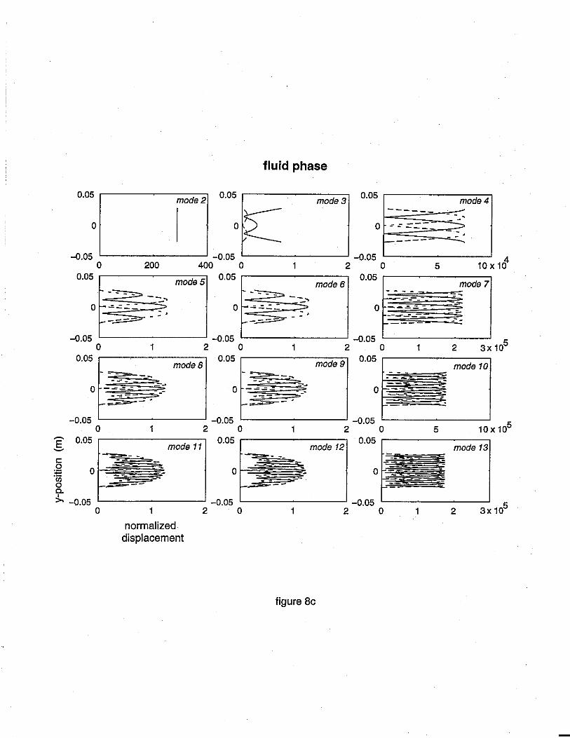
0.05

0

-0.05 0

0.05 200

"~-----:., ... 0 ~ - - ----

.. ; I -----0.05

0 1

fluid phase

mode2 0.05

mode3

0~

-0.05 400 0 2

modes 0.05 ---------mode6

-0.05 2 0 2

0.05 --------- 0.05 mode9

-~------ - --0 -..z:-=-= --- -= -

1-- - ..

-0.05 0 1

E o.o5 ~

C .Q

-~ 0..

'

o~--~.._ ---- - --,_ --

modeB

2

mode 11

-~ ----- - --0 --~-= ~-... -=-1-- - ..

-0.05 0 2

0.05 --------­mode 12

0~ 1-~

0.05 mode4

.

- -0 ~:

L- --0.05

10 X 1& 0 5 0.05 ---------

-0.05 0 1 2 3x 105

0.05 mode 10

0

-0.05 0 5 10 X 105

0.05 ---------mode 13

--0

->- -0.05 L_ _______ __, -0.05 L----------' -0.05 L---~--~--3--'x 105

0 2 0 1 2 0 1 2

normalized displacement

figure 8c

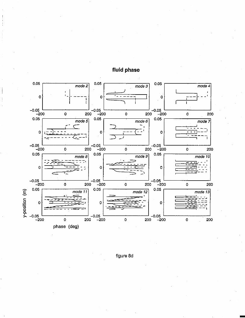
fluid phase

0·05 .--------m-od_e_2~ 0·05 .-------m-o_d_e_3~ 0·05 .--------m-o-de~4

0 0 -=: =·=· - =::(:------t-: -----'

.

0 ~--: -0.05 -0.05 '---------' -0.05

-200 0 200 -200 0 200 -200 0 200 0

·05 mode 5 °·05 mode 6 °·05 mode 7 ,-~ 0 I - _;} - :: :: __ ~ __

·-==---- - - - ~--' ,--{--' )

0 - --, ------

I

-0.05 '----------' -0.05 -------~ -0.05 ~-------~ -200 0 200 -200 0 200 -200 0 200

0·05 .--------m-o-de-8~ o.o5 .-------m-o_d_e_9~ 0·05 .-------m-o_d_e_1~0

-·-~ - ------, 0 - - -= -'_ ... Jf -_ -,

,_ 0

- - - ' - - ' - - -- - --- -

-0.05 '----------' -0.05 '---------' -0.05 -200 0 200 -200 0 200 -200 0 200

E o.o5 mode 11 °·05 ,-------m-o-de-12~ 0·05 mode 13

~

r:: 0

:;::: ·;;; g_

0 .-§~2-~~z-~ --~ 0

>, -0.05 '---------' -0.05 '---------' -0.05 -200 0 200 -200 0 200 -200

phase (deg)

figure 8d

- - ---~ - -----_-_-_:i ---,

0 200

-

~

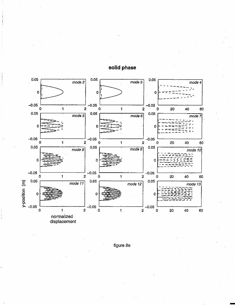
E ~

C: 0 :E ~ C.

0.05 ---------~ mode2

solid phase

0.05 ---------­mode 3

0

0.05 --------d,-­mo e4

- - - - --,. ___ -.. 0 I.------ - - -- - - ------~----- - - - -

-0.05 L_ _______ ___, -0.05 '----------' -0.05 0 1 2 0 1 2 0 20 40 60

0·05 -------m-od_e_5 0·05 _______ m_o_d,_e_6_ 0·05 .-------m-o_d,_e~7

---~ -- = - - - -0 I- - -- - 0 :-__ : -

------ --0.05 -0.05 '----------' -0.05

0 1 2 0 1 2 0 20 40 60 0.05 modeB 0.05 mode9 0.05 ----------mode 10 - - - ------ ---

0 - - -- - -=- 0 ~. =--· o~gJJJ}¥-:

-0.05 -0.05 '-----------J -0.05 '---~------' 0 1 2 0 1 2 0 20 40 60

0.05 mode 11 0.05 mode 12

0.05 ----------mode 13

0 0

:!,., -0.05 ._ ________ _, -0.05 '----------' -0.05 '---~------0 1 2 0 1 2 0 20 40 60

normalized displacement

figure Be

-

0·05 ~------m-o-de-2~

0

solid phase

0·05 ~------m-o-de_3_

0 ]-----7 0·05 ~------m-o-de-4

0 :--2 -0.05 c_ _______ _., -0.05 ~-------~ -0.05 .__ _______ _.,

-200 0 200 -200 0 200 -200 0 200 o.o5 mode 5 °·05 ~-----m-od_e_6_

0 2 ', - - - -t1 0

0.05 ~-------~ model

·--~ o,~~~

-0.05 '-----------' -0.05 ~-------- -0.05 L,_ _______ __J

-200 0 200 -200 0 200 -200 0 200 0.05 0.05 ~-------~

modeB mode9 0.05 ______ m_o_d_e-10-

:~-- -j: - 0 ~--t===---===7"'~§ -0 -~----L-- - -

0 ------L__ - - • ,----- --0.05 L,_ _______ _j -0.05 ~-------~ -0.05 L,_ _______ __J

-200 0 200 -200 0 200 -200 0 200 E o.o5 0.05 ~-------~

mode 12 0·05 ~-----m-o_d_e-13-

0 ~·1:;g-_ ~

C: 0 0 :E en 0

~-----~%:--=-, J 0 '. :--=---=---=--~:::

C. >, -0.05 '---------....J -0.05 ~-------~ -0.05

-200 0 200 -200 0 200 -200 0 200

phase (deg)

figure Bf

fluid phase

0·05 ,--------m-od_e_2~ 0·05 _______ m_o_d_e_3 0.05

o~~ 0

--0 "So - --

--0.05 '----------' -0.05 '----------' -0.05

0 20 40 0 1 2 0 2

mode4

----

4 4x10

0.05 mode5 °·05 mode6 0·05 ,--------m-od-e~7

-~----:: > 0 ·~-=..::-= - -- -.... --- ~

--- -­_, 0 - .... .:..:.=. - -- ---- ~

------...---- --~

0 ------- --

-- - - -5 -0.05 '----------' -0.05 -0.05

0 1 2 0 1 2 0 1 2X 10 o.o5 _______ m_o_d_e_B~ 0·05 _______ m_o_d_e_9 0.05

0

-0.05 '----------' -0.05 '----------' -0.05 0 2 0 2 0

----=-

2

mode 10

5 4X 10

E o.o5 mode 11 °·05 ______ m_o_d_e-12- 0.05 ,---------~ mode 13

~

C 0

:;:,

'8 C.

>- -0.05 '----------' -0.05 '----------' -0.05 0 1

normalized displacement

2 0 1 2 0

figure Bg

2 5

5X 10

fluid phase

0.05 mode2 0.05 mode3 0·05 ,--------m-o-de-4-,

0 :_ -~--7 0 0 : __ ~

-0.05 -0.05 ~-------~ -0.05 -200 0 200 -200 0 200 -200 0 200

0.05 mode5 0.05 mode6 0·05 ,-------m-od_e_7-,

-~ 0 ,--:z---' 0

~-,--{--' )

0 ,---~----- - - ---- - -I

-0.05 -0.05 ~------~ -0.05 ~--------' -200 0 200 -200 0 200 -200 0 200

0·05 ,--------m-o-de-8~ 0·05 ------m-od_e_9~ 0·05 ,-------m-o_d_e_1-,0

o::~s-~~~ =- 0

-0.05 ~--------' -0.05 ~-------~ -0.05 -200 0 200 -200 0 200 -200

'---~--' - - -­- - - ---- - - --- -----

0 200

:[ 0.05 mode 11 0.05 mode 12 0·05 ,-------m-o-de-13-,

C: 0

:;::: -~ C.

,- ~ ~ -0 :i!= =-- ~ ~c- ~ 0 ~ii=_w- r; ~:

- - - :.,

0 ---~--\.-------- - - - ----- - -

i::..,-_-_ - -_ -_ r-- -- -

>- -0.05 ~--------' -0.05 ~------~ -0.05 ~--------' -200 0 200 -200 0 200 -200 0 200

phase (deg)

figure 8h

C:

0·05 ~------m-od_e_2-,

0 ' )

-0.05 0 2

0.05 ~--------, mode5 - - -~-

o ~- --- ~ ---·----i; -

-0.05 0 2

0.05 ---------, modeB

--

solid phase

0·05 _______ m_o_d_e-,3 0·05 -------m-od_e_4.,

-0.05

0.05

0

-0.05

0.05

0

--- - - - -- - - -----~

0 ~ ------ -:.------ - - :.

~-------~ -0.05 ~-------~ 0 1

- .. ..::,_ --~-: ~

----

2 0 10 20

mode6 0·05 ~------m-o-de~7

0 ~:~::~-=-==::; 1-..--_- ~ -- _- _- ..

-----'----------' -0.05 0

~ -- --- --

1 2 0 10 20 0·05 -------m-o-de-10-, mode9

-0.05 '-----------' -0.05 '------------' -0.05

0.05 0 2 0 1 2 0 10 20

mode 11 0.05 ---------,

mode 12 0·05 ------m-od-e-13.,

g 0 0 "iii 0 C. >- -0.05 '--------~ -0.05 '------------' -0.05

0 1 2 0 1 2 0

normalized displacement

figure 8i

10 20

-

0.05 ---------mode2

0 ( ----- - -I \

0.05

0

solid phase

mode3

J---- ---------,

I I

0·05 -------m-o-de-4

o c_---~----, -0.05 L_ _______ _, -0.05 '--------~ -0.05 .__ _______ _,

-200 0 200 -200 0 200 -200 0 200

o.o5 mode 5 o.o5 mode 6 0·05 -------m-o-de-7

0 l :_ ·_ --t-1_ 0 o:=:~ -0.05 L_ _______ _, -0.05 '--------~ -0.05

-200 0 200 -200 0 200 -200 0 200 0.05 mode B 0.05 ------m-od_e_9~ 0.05 mode 10

0 -:·- ----j--'

0 0 ,"c------------

~--5-~ -0.05 L_ _______ _, -0.05 '--------~ -0.05 '---------'

-200 0 200 -200 0 200 -200 0 200 E o.o5 mode 11 0·05 ______ m_o_d_e-12- 0·05 ______ m_o_d_e_1_3 ~

C: 0 :E gi C.

0 0 . -~--~;0- ;-=--=--=--~ 0 ::~~~~

>- -0.05 L_ _______ _, -0.05 '--------~ -0,05 '----------' -200 0 200 -200 0 200 -200 0 200

phase (deg)

figure Bj

-

C:

fluid phase

0.05 mode2 0·05 _______ m_o_d_e~3 o.o5 r-------m-o-d7 e-4""

I ( 0

---f-========-- - ---o - • - :: --=2. __

-0.05

0.05

-~-------~ -0.05 ~-------~ -0.05

0 10

t-----= - --

20 0 2 0

mode 5 o.o5 mode 6 o.o5

-0.05 ~-------~ -0.05 ~-------~ -0.05 0 2 0 2 0

0·05 r-------m-o_d_e_B~ 0.05 _______ m_o_d_e_9~ 0.05

0 --.:._ -

--- - -

100 200

500

--

model

1000

mode 10

-0.05 ~-------~ -0.05 ~-------~ -0.05 ~-------~ 0 1 2 0 1 2 0 1000 2000

0·05 -------m-o-de-1~1 0·05 ______ m_o_d_e_1~2 0·05 -------m-o-de-13~

- -,g 0 0 'iii g_ >- -0.05 ~-------~ -0.05 ~-------~ -0.05

0 1

normalized displacement

2 0 1 2 0

figure Bk

1000 2000

-

fluid phase

0.05 0.05 0.05

0 ;_ ----t\ 0 }'· -----7 0 :_~ -0.05 -0.05 -0.05

-200 0 200 -200 0 200 -200 0 200 0.05 0.05 0.05

0 -_·_ E--:_ 0 1--~------ - ---- - - -I

-0.05 ~-------~ -0.05 ~-------~ -0.05 ~-------~ -200 0 200 -200 0 200 -200 0 200

0.05 --------~ 0.05 0.05 --------~

0 - - -,.-=--=-3- -_ ~ --= -------,

,_ -~ - -~ -0 L:: ;:=.-.;::.._.:,

==-= -= = ~ =.i :;;: 0

-0.05 ~-------~ -0.05 ~-------~ -0.05 -200 0 200 -200 0 200 -200

, __ -~--I - - -­- - - ---- - - --- -----

0 200 E o.o5 0.05 0.05 --------~ ~

C: 0 :,= ·;;; 0 C.

0

:!,., -0.05 ~-------~ -0.05 -------~ -0.05 -200 0 200 -200 0 200 -200

phase (deg)

figure Bl

---~----' I------- - - - ------ - -r::_-_-_ - -_ -_ r-- -- ..

0 200

-

jrop 0h 0 0 Do1 Doz Do3 -jrop 0h

0 jrop 0h 0 D21 D22 D23 0

0 0 jrop 0h D41 D42 D43 0

jropo(l-h) 0 0 Eo1 Eo2 E03 B10 -jrop 0 (1-h)

0 jrop 0 (1-h) 0 E21 E22 E23 B12 0

0 0 jrop 0 (I-h) E41 £42 E43 B14 0

= ikoxo 0 0 Fo1 Fo2 Fo3 A11 jko

0 jkox2 0 F21 F22 F23 A12 0

0 0 ikox4 F41 F42 F43 A13 0

0 0 0 G21 G22 G23 0

0 0 0 G41 G42 G43 0

0 0 0 G61 G62 063 0

figure 9

-

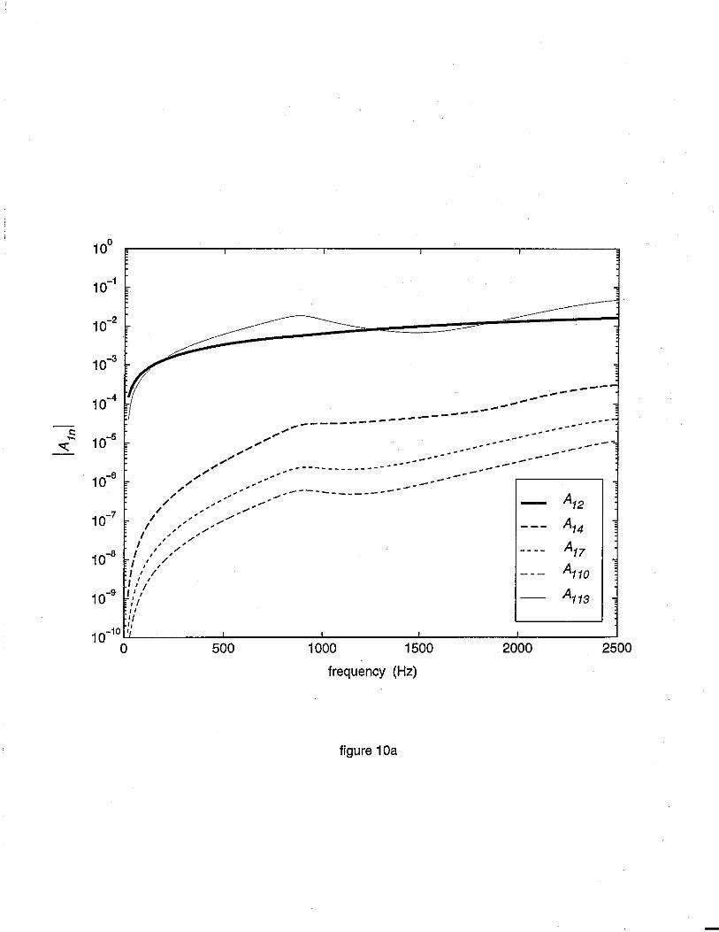
C: -<:(

10-3

.,,.,,,,,,; _,.;

.,, ,'

/ _, I/ ,., ....

I ,.,' .,,, .. .,,,.,,..,,, I , ,,,_..

I , '

10-a I ,' ,,,.

/ / ,/

I ' / I ' '

9 '

,' / 10- ,' ,'

-----------------------.,,..--------.,,,.,.,.,,,."'

--------------------------- --... ------------------

,r r

r

---------------

--------------- -------------

A12

A14

A17

A110

A113

" 'I ,, 1 o-10 '"'''---'------'---------'-------'--------'----------'

0 500 1000 1500 2000 2500

frequency (Hz)

figure 10a

10°

10-1

10-2

10-3

10-4

C: 10-5 -__:L

10-6

10-7

10-8

10-9

10-10 0 500

-----==---=---------------------- --- ---~~::...-:--.::--------

1000

----.. , ----- .,.,,,. .. >,;,. __ ...-- ,, A

- - - - , ' 13 \ / ,_,'

1500 2000

At5

At6

AtB

At9

Attt

A112

frequency (Hz)

figure 10b

2500

-

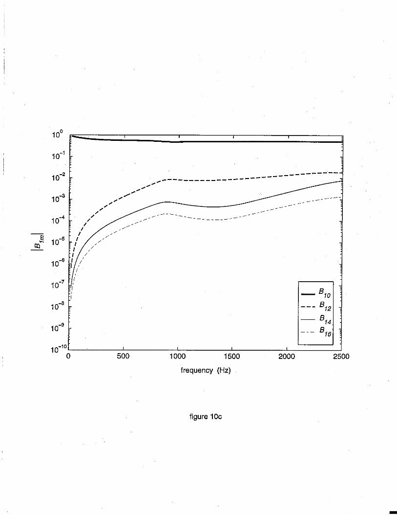
E: -ca

10°

10-1

10-2

10-3

10-4 / I

I I

10-5 I I I I

10-6 I

10-7 ' I

I

I

' I

/ , I ,

-------...... ...... ... ...--...

-----------.,,,,..,,,,.- ---------... ... .,, ,, ,,

-----//

/

/

/ , /

10-10'--~----'-------L-------'--------L-------' 0 500 1000 1500 2000 2500

frequency (Hz)

figure 10c

-

g

20Hz 200Hz 2000Hz

0.05 --------- 0.05 -------~ 0.05 ---------

--

-0.05 0

0

--­; 0 -

--­__ .,

-0.05 '----------' -0.05 '-----------' 2x10-6 0 4x10-5 o 4x10-4

0.05 -------~

0

0.05 ---------

\ ,, 0 '

,/ ) -0.05 L, _______ _, -0.05 .__ ______ __, -0.05 L, _______ _.

0 0.001 0 0.002 0 0.002

0.05 0.05 ---------

,:: 0 E 0 0

\ ,, 0 \ ) ~

C. 1/ >,

-0.05 L, _______ _. -0.05 '----------' -0.05 0 0.001 0 0.002 0 0.002

displacement (m)

figure 11 a

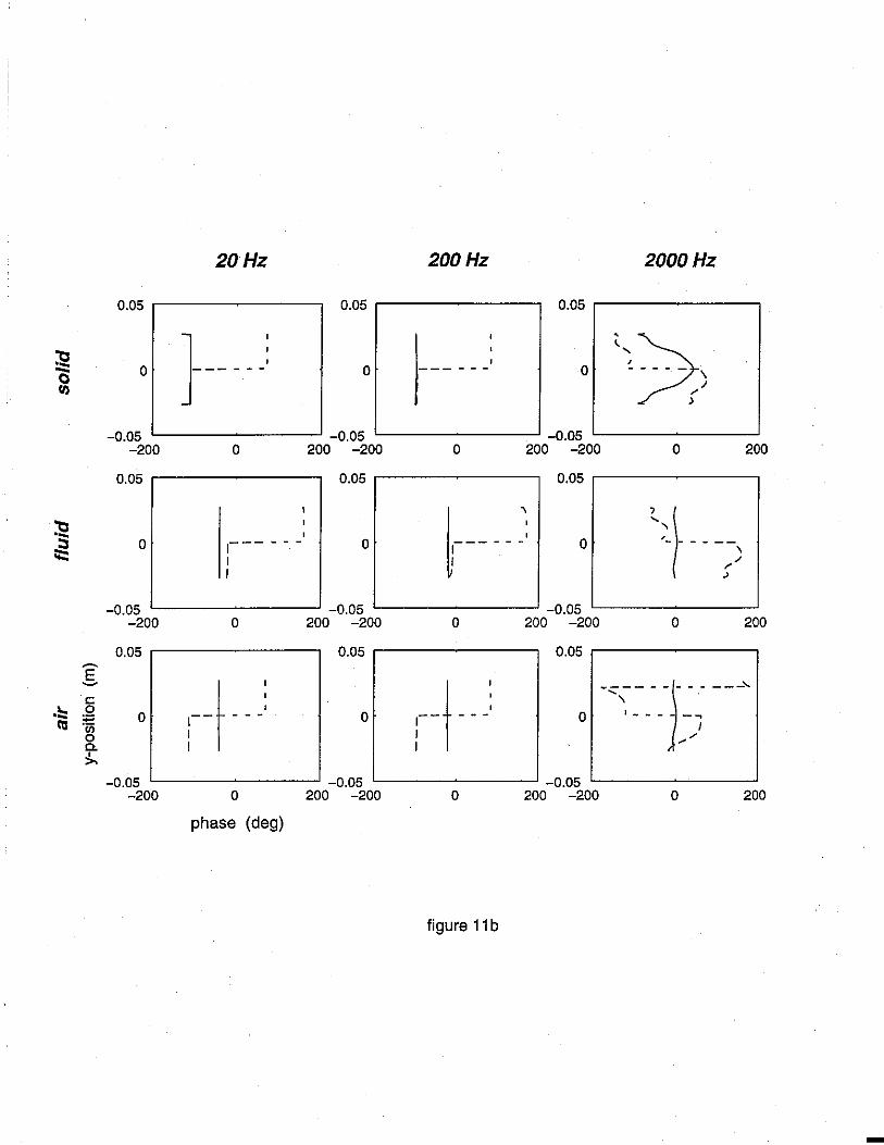
20Hz 200Hz 2000Hz

0.05 0.05 0.05

;g 0 ]--- - - 0 --- - - - 0 \>) 0

II)

-0.05 -0.05 -0.05 -200 0 200 -200 0 200 -200 0 200

0.05 0.05 0.05

!;! 1-----; '~t- -? :::s 0 i--- - - - 0 0 :;:: I

I

-0.05 -0.05 -0.05 -200 0 200 -200 0 200 -200 0 200

0.05 0.05 0.05 ~

E

:--t--- :--t---: ~ ---- -r- --~ C: ', .

·== 0

0 0 0 1 ___ --,

:;::: Ill 'iii J

0 ~,,. C. ' >-

-0.05 -0.05 -0.05 -200 0 200 -200 0 200 -200 0 200

phase (deg)

figure 11 b

-

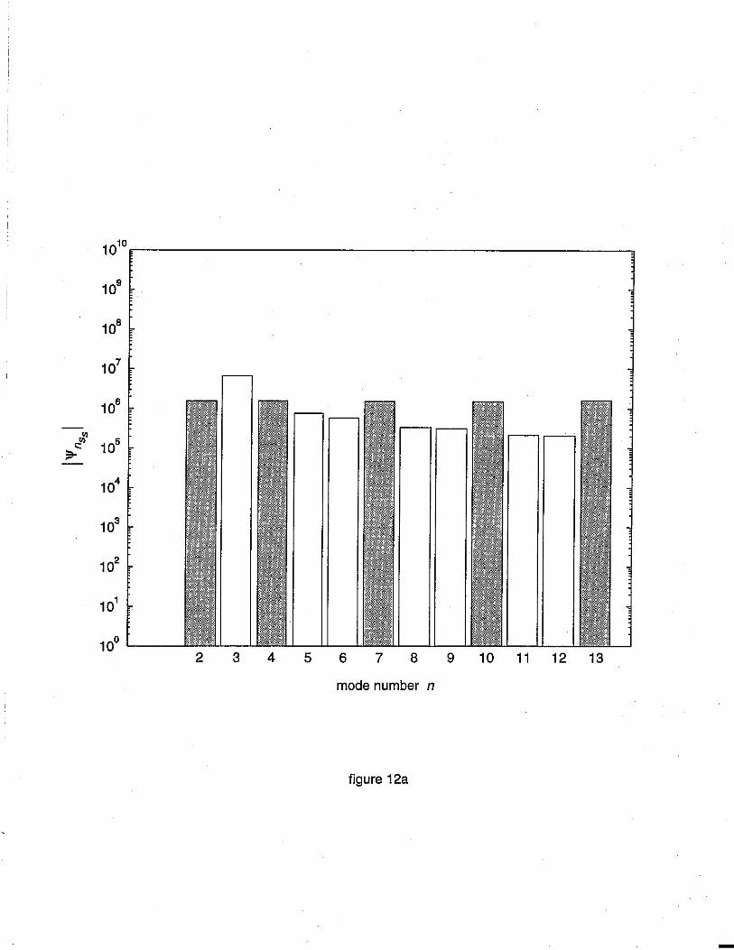
1010

109

108

107

106

c:..y; 10

5 )3-

104

103

102

101

10° 2 3 4 5 6 7 8 9 10 11 12 13

mode number n

figure 12a

1010

109

108

107

106

--~ to

105

;:r C:

104

103

102

101

10° 2 3 4 5 6 7 8 9 10 11 12 13

mode number n

figure 12b

-

1010.-----------------------------~

1 o0 '----

2 3 4 5 6 7 8 9 10 11 12 13

mode number n

figure 12c

5~-----~-----~-----~-----~------I \ I

4 I

3

2

1

I \

' , ... ---

porous half-space constrained-edge : 1 air mode & 3 foam modes constrained-edge : 2 air modes & 6 foam modes constrained-edge : 3 air modes & 9 foam modes constrained-edge : 4 air modes & 12 foam modes

0f----------------------------------l

I I

I I I I

I I

I

'""===----------===-=--'-"-,.-=-.:-a,;-9 -------~ ---,,,,...,,..,,,,,.-

/ --~---/

_3LL.J__ ___ _,__ _____ .J__ ____ _J_ _____ --'-____ __J

0 500 1000 1500 2000 2500

frequency (Hz)

figure 13

1.----------,-------,------~-----~----~

0.9

0.8

0.7

0.6

0.5

0.4

0.3

0.2

0.1

I I

I I

I I I I I I

I

/ I

,,.,--/

---- ,r' ------------ 1/

porous half-space constrained-edge : 1 air mode & 3 foam modes constrained-edge : 2 air modes & 6 foam modes constrained-edge : 3 air modes & 9 foam modes constrained-edge : 4 air modes & 12 foam modes

0'-------"-------'-------'--------'---~------' 0 500 1000 1500 2000 2500

frequency (Hz)

figure 14

-

0 ' ?---~ ' ' -------------50- .

-100- .

-150'" .

~ -200'" , . ~ I 'E / ~

.,, - -250'" --"<" / -E

-300- -

-350- .

-400

-450 ' . , ,

-500 ' ' ' ' ' -100 -50 0 50 100 150 200

Re {k } (m-1) X

figure 15

-

5 r-ir---r-----r-----r------.------,-----,-----,---~-----~ I I I

4 I

3

£ 2

1

I \

' , __

-------------------------------

porous half-space

constrained-edge : 2 air modes & 6 foam modes

01--------------------------------l

I I

I I

I

/ I

I

/

.,,,-.,

----------------------------------------

_3LL-'----'---...L---'---L-----'---....L.---'----'--__JL-_.....J 0 200 400 600 800 1000 1200 1400 1600 1800 2000

frequency (Hz)

figure 16

-

1.------,------,---,------,----,--~----.----,-----~

0.9

0.8

0.7

0.6

0.5

0.4

0.3

0.2

0.1

I I

I I I I I I

I

/ I

I

/

,.-­/

---------------------

porous half-space

constrained-edge : 2 air modes & 6 foam modes

0L----'----'----'----'----'----L---'----'---_,_---0 200 400 600 800 1000 1200 1400 1600 1800 2000

frequency (Hz)

figure 17