The effect of green time on stochastic queues at traffic signals

Nicholas B. Taylor* and Benjamin G. Heydecker

Centre for Transport Studies, University College London, Gower Street, London WC1E 6BT, UK

(Received 10 March 2013; accepted 25 July 2013)

Many analyses of traffic signal queues use Webster and Cobbe’s formula, whichcombines the net effect of the red/green cycle with a term representing stochasticeffects, idealised as an M/D/1 queue process having random arrivals and uniformservice. Several authors have noted that this component should depend not only ondemand intensity but also on throughput capacity in each green period, although anextra empirical term may partially allow for this. Extending the service interval in M/D/1 (M = Markovian, i.e. random, D = deterministic, i.e. uniform, 1 = one server)enables the effect to be reproduced, but no exact expressions for its moments arefound. Approximate formulae for the extended mean exist but are accurate only nearsaturation. The paper derives novel approximations for the equilibrium mean and alsovariance and utilisation, using functions linking traffic intensity with green periodcapacity. With three moments, equilibrium probability distributions can be estimatedfor which a method based on a doubly nested geometric distribution is described.

Keywords: signal; queue; stochastic; M/D/1; variance; probability distribution

Introduction and background

Real signalised junctions are complicated by demand-responsive timings, conflictingmovements and coordination. Microscopic simulation, which need only specify short-termindividual behaviour, is used increasingly. Nevertheless, the formula of Webster andCobbe (1966) for queue size or delay at an isolated signal is still widely regarded. Inaddition to red and green phase component, it contains a term representing stochasticeffects, including transient overload. This is equivalent to an idealised queuing processwhere customers arrive randomly and are served at uniform intervals. Several authors,including Olszewski (1990), have pointed out that this overestimates the true stochasticqueue component, which simulation shows falls, albeit slowly, with increasing throughputcapacity in the green period. Webster’s formula has an empirical term that may compensatefor this effect and can be related to a more exact formula. However, it is difficult tointegrate these with computationally efficient time-dependent approximate methods.

After describing the basic stochastic process, an extension is developed to takeaccount of green period capacity. Simulation results based on it are used to deriveapproximations to the queue’s equilibrium utilisation, mean and variance in formscompatible with time-dependent queuing methods, which are shown to be moreconsistent than earlier empirical approximations. A novel approach makes use of linkfunctions between traffic intensity and green period capacity, allowing a broad physical

*Corresponding author. Email: nicholas.b.taylor@ucl.ac.uk

Transportation Planning and Technology, 2014Vol. 37, No. 1, 3–19, http://dx.doi.org/10.1080/03081060.2013.844907

© 2013 The Author(s). Published by Taylor & Francis.This is an Open Access article distributed under the terms of the Creative Commons Attribution License (http://creativecommons.org/licenses/by/3.0), which permits unrestricted use, distribution, and reproduction in any medium, provided the original work isproperly cited. The moral rights of the named author(s) have been asserted.

interpretation. Comparison with simulation shows that the results are accurate over arange of traffic intensities and green period capacities. A method of estimating aprobability distribution from the three moments is described that may have widerapplication. Finally, the theoretical nature of the analysis is justified, and variousconceptual and practical issues are discussed.

The mean queue size at a signal

Allsop and Hutchinson (1972) trace the origins of signal queue analysis back to A J HClayton in 1940, as well as discuss the impact of different assumptions about arrivalpatterns. A well-established expression for the mean queue size L at a fixed-time trafficsignal is Equation (1), ascribed to Webster (Webster and Cobbe 1966):

L ¼ LP þ LV þ LW ¼ xlc 1� Kð Þ22 1� xKð Þ þ x2

2 1� xð Þ � 0.65 xlcð Þ13 x 2þ5Kð Þ ð1Þ

The queue size in vehicles is composed of a phase term LP visualised as growing linearlyduring the red phase and discharging linearly and fully during green, a stochastic andoverload term LV, and an empirical adjustment LW. Other variables are defined below asfollows:

c signal cycle time;g green time within each cycle;r red time within cycle;Λ green cycle time ratio = g/c (avoiding possible confusion with demand rate λ);s saturation flow, the maximum flow rate across the stop-line;µ = gs/c, capacity of the movement taking account of the green/cycle ratio;x average degree of saturation or utilisation of service at the stop-line.

Webster’s formula strictly applies to Poisson arrivals at an isolated signal, so excludesfactors like minimum headway, vehicle actuation, platooning and coordination. However,the concern here is solely with the effect of green capacity on the stochastic term and itsform in relation to existing time-dependent methods. Other variables used in the paper arethe following:

G = gs = µc, the number of vehicles1 that can pass in a single green periodρ = λ/µ, demand intensity, relative to capacity

Note that G is present effectively as µc in the first and last terms of Equation (1) but notthe stochastic term. The degree of saturation x cannot exceed 1, so only the stochasticterm can accommodate indefinite queue growth and then in principle only by being time-dependent. A more integrated approach is the derivation from first principles ofHeidemann (1994), using a generating function and the results of Meissl (1963).Heidemann shows this gives results imperceptibly different from Webster and Cobbe’s forvalues of G up to 45. If equilibrium conditions are imposed, the queue formula can bereduced to a form analogous to Equation (1) containing the identical phase term LP:

L ¼ LP þ LV G½ � þ LH where LH ¼ �K 1� xð Þ 2LV G½ � þ Kx� �þ Kx

2 1� Kxð Þ ð2Þ

4 N.B. Taylor and B.G. Heydecker

The ‘exact’ stochastic term LV[G] here is a complicated expression that requires numericalevaluation of the roots of a function of degree G. However, when G = 1 it reduces to LV.The third term, LH, is free of empirical constants, and test calculations suggest it isgenerally small. However, Equation (2) is again inconvenient for time-dependent trafficmodelling because of the intractable stochastic term, so a simpler expression is sought.

Dependence of the stochastic queue on green period capacity

Olszewski (1990) uses Markov simulation based on transition probabilities, allowing fora general arrival distribution and variable cycle time, to confirm observations by Newell(1965) and Miller (1969) that the mean size of the stochastic queue at a signal decreasessystematically with increasing green period capacity2 G. Although the decline is gradual,it can be substantial for long green times, and this trend appears to continue indefinitely.For example, at 90% saturation (x = 0.9), the mean queue with 40 second green is halfthat with a short (1–2 second) green. The US Highway Capacity Manual (HCM)(Rouphail, Tarko, and Li 1996) and Australian time-dependent formulae (Akçelik 1998)also contain empirical terms depending on green period capacity. Olszewski’s Figure 33

shows that his EVOL simulation results compare well with Newell’s formula, though lesswell with Akçelik’s.

Some fundamental properties of queues and time-dependent approximation

All queues obey the time-dependent deterministic Equation (3) representing conservationof units (customers, vehicles etc.), where L0 is the initial queue and x is the averageutilisation or degree of saturation over the period of development [0,t]. If the demandintensity ρ < 1, the mean queue tends to an equilibrium value given by the Pollaczek–Khinchin (P–K) mean queue formula (4) (e.g. Kleinrock 1975):

Ld x,tð Þ ¼ L0 þ q� xð Þlt ð3Þ

Le xð Þ ¼ Ixþ Cx2

1� xð4Þ

For equilibrium to exist, Equation (4) must be finite, so Equation (3) must also remainfinite at equilibrium, implying that ρ < 1 and x → ρ. Service occurs only when a queueis present, so at equilibrium, the average probability that the queue is zero is thecomplement of the utilisation:

�p0e ¼ 1� q ð5Þ

Utilisation x represents the proportion of time that a queue is present at the stop-line or inservice. The forms of Equations (3–4) show that it plays a crucial role in queuedevelopment, being the only quantity on the RHS that must vary with time and is capablein principle of producing any finite size of queue.

The coefficient I in Equation (4) reflects unavoidable service time, which convention-ally applies only to priority junctions, while C depends on the coefficient of variation ofservice time.4 For a signal I = 0, while theoretically C = 0.5, giving LV as in Equation (1).

Transportation Planning and Technology 5

Empirically, C is found to be in the range of 0.5–0.6 (Burrow 1987). When Equations (3)and (4) are equated and solved for x or L, the result is the quasi-static ‘sheared’approximation to time-dependent queuing, including stochastic effects, being defined forall ρ, since x never exceeds 1 (e.g. Kimber and Hollis 1979). This has some accuracy issuesbut is convenient for use in dynamic network assignment programs such as CONTRAM(Taylor 2003). Shearing the entire signal queue formula is problematic, as found by Han(1996). However, the methods described so far do not provide all the moments needed todetermine queue size probability distributions, enabling the risk of long tailbacks, orspillback across upstream facilities, to be estimated. The rest of the paper, therefore, aimsto obtain variance along with mean.

The M/D/1 process as an idealisation of the stochastic queue at a signal

The M/D/1 queue (M = Markovian, i.e. random, D = deterministic, i.e. uniform, 1 = oneserver) represents an idealised system where customers are served singly, but more thanone random arrival can take place in each fixed average service time interval 1/µ. Theeffect of overflow from the red/green signal cycle is averaged out. In the M/M/1 process,by contrast, arrivals and service both occur randomly at given mean rates, which is moretypical of a priority junction. Each process can be described by recurrence relationsbetween queue state probabilities, which can be animated as Markov processes (Kendall1951). Both yield closed-form equilibrium moments, including means in the P–K formEquation (4), making them convenient for use in time-dependent traffic modelling.

Arrivals at exponentially distributed random intervals result in the number of arrivals ineach service period being Poisson distributed. For M/D/1, the probability of i customersbeing in the queue after µt + 1 service periods (i.e. that amount of throughput capacity) isthe sum of the probabilities of i + 1 being in the queue at service point µt and no arrivals inthe interval [µt, µt +1), i at µt and one arrival, i − 1 at µt with two arrivals, and so on.Hence, the probabilities of queue states {pi} where i={0,1,2,…} evolve according to:

pi lt þ 1ð Þ ¼Xiþ1

j¼0

qje�q

j!piþ1�j ltð Þ ð6Þ

Dpi ltð Þ ¼ pi lt þ 1ð Þ � pi ltð Þ ð7Þ

At equilibrium, by definition, Δpi(µt) = 0 for all i, so rearranging Equation (6) and allowingfor the ‘absorbing barrier’ at i = 0, which corresponds to periods when the queue is zero andservice is not utilised, the following equilibrium recurrence relations are obtained:

p1 ¼ eq � q� 1ð Þp0 ð8Þ

pi ¼ eq � qð Þpi�1 �Xij¼2

qj

j!pi�j ði > 1Þ ð9Þ

The first two terms in Equation (8) come from Equation (6) with i = 0, while the third canbe obtained from Equation (6) by setting i = −1 (notional ‘negative queue states’ feature

6 N.B. Taylor and B.G. Heydecker

prominently later, and are discussed at the end of the paper). Moments of the equilibriumdistribution can now be got from Equations (8–9) by evaluating the next highest time-dependent moment in each case:

Probability of zero queue by evaluatingX1i¼0

ipi : p0e ¼ eq 1� qð Þ ð10Þ

Mean queue by evaluatingX1i¼0

i2pi : Le ¼ q2

2 1� qð Þ ð11Þ

Variance by evaluatingX1i¼0

i3pi : Ve ¼ q2 6� 2q� q2ð Þ12 1� qð Þ ð12Þ

The form of Equation (11) is that of the stochastic queue LV in Equation (1) and is aparticular case of Equation (4). However, Equation (10) is inconsistent with Equation (5).This is because it applies at the end of the green period, at which time, p0 will be greatestsince it excludes transient queues that have come and gone during the green period. Thatthe end-of-green p0e is always greater than the average-over-green �p0e (since eρ ≥ 1) isconsistent with this interpretation. This distinction does not arise where a queuing processcan be formulated using infinitesimal service periods, as in the case of M/M/1.

Extending the M/D/1 queue process to general green period capacities

In this paper, we use a common subscript notation for queue moments, where e indicatesequilibrium, [G] is added to indicate the dependence on green period capacity and ifomitted G = 1 is assumed, and a final letter, e.g. M, distinguishes a particular origin, forexample, the initial of an author, while an overscore indicates an average value andnotional negative queue state indices are placed in brackets.

The basic M/D/1 process describes a situation where only one customer can be servedin each green period (like a ramp-metre with a fixed cycle time). A more realistic model

Table 1. Conditions for specified final queue in green period with capacity G.

Initial queue state Arrivals in green period

Zero queue i = 0 at end of green period0 Up to G1 Up to G−1J Up to G−j>G Not possible

Non-zero queue i > 0 at end of green period0 Exactly G + i1 Exactly G−1 + iJ Exactly G−j + i>G+i Not possible

Transportation Planning and Technology 7

should allow up to G customers to be serviced in each green period in which case theconditions for final queues of specified sizes are as given in Table 1.

Table 1 suggests that while the development of the queue size probability distribution{pi} for i >> 0 will be broadly similar to Equation (6), the expression for p0 will be morecomplicated, involving several components. Cronjé (1983b) introduces negative netcontributions in each cycle, from −G to 0, representing actual arrivals minus green periodcapacity and sums these terms to give the value of p0 at the end of the cycle. Thisamounts effectively to employing notional negative queue states down to −G. By asimilar analysis to that for M/D/1, recurrence relations corresponding to Equations (6–9)are obtained:

pi lt þ Gð Þ ¼XiþG

j¼0

Gqð Þje�Gq

j!piþG�j ltð Þ ði � �GÞ ð13Þ

The presence of G on the LHS and the substitution of Gρ for ρ on the RHS reflect the factthat all calculations relate to an idealised service period of G/µ in place of 1/µ. Equation(13) is valid for the notional states provided these include a notional zero state. The real(absorbing) zero state probability is got by summing all the notional probabilities,including (0), Equation (14) and states I > G can be expressed in terms of real statesalone:

p0 ¼Xi¼0

i¼�G

p �ið Þ ð14Þ

pi ¼ eGqpðeÞi�G �Xij¼1

Gqð Þjj!

pi�j ði>GÞ ð15Þ

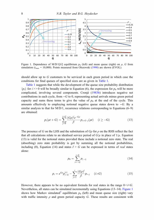
However, there appears to be no equivalent formula for real states in the range 0< i<G.Nevertheless, all states can be simulated incrementally using Equations (13–14). Figure 1shows how Markov simulated5 equilibrium p0 (left) and mean queue size (right) varywith traffic intensity ρ and green period capacity G. These results are consistent with

1

0.9

0.8

0.7

0.6

0.5

0.4

0.3

0.2

0.1

p 0

00 10 20 30 40 50

G60 70 80 90 100

0.25

r

r

0.40.50.60.70.80.9

0.25

r increasing

r increasing

0.40.50.60.70.80.9

00

0.5

1

1.5

2

2.5

3

L e_M

/D/1

[G] 3.5

4

4.5

5

10 20 30 40 50G

60 70 80 90 100

Figure 1. Dependence of M/D/1[G] equilibrium p0 (left) and mean queue (right) on ρ, G fromsimulation (imax = 10,000). Points measured from Olszewski (1990) are shown (EVOL).

8 N.B. Taylor and B.G. Heydecker

there being no positive lower limit on the mean queue size as G is increased (in practice,of course, delay on conflicting streams facing long red times might outweigh this!).

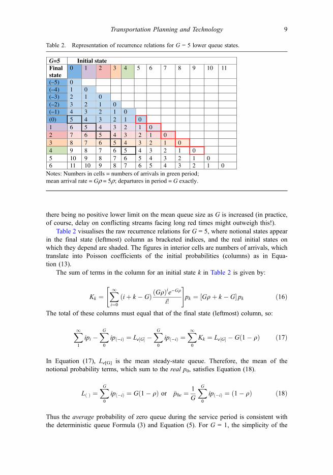
Table 2 visualises the raw recurrence relations for G = 5, where notional states appearin the final state (leftmost) column as bracketed indices, and the real initial states onwhich they depend are shaded. The figures in interior cells are numbers of arrivals, whichtranslate into Poisson coefficients of the initial probabilities (columns) as in Equa-tion (13).

The sum of terms in the column for an initial state k in Table 2 is given by:

Kk ¼X1i¼0

ðiþ k � GÞ Gqð Þie�Gq

i!

" #pk ¼ Gqþ k � G½ � pk ð16Þ

The total of these columns must equal that of the final state (leftmost) column, so:

X11

ipi �XG0

ip �ið Þ ¼ Le G½ � �XG0

ip �ið Þ ¼X10

Kk ¼ Le G½ � � G 1� qð Þ ð17Þ

In Equation (17), Le[G] is the mean steady-state queue. Therefore, the mean of thenotional probability terms, which sum to the real p0, satisfies Equation (18).

Lð Þ ¼XG0

ip �ið Þ ¼ G 1� qð Þ or �p0e ¼ 1

G

XG0

ip �ið Þ ¼ 1� qð Þ ð18Þ

Thus the average probability of zero queue during the service period is consistent withthe deterministic queue Formula (3) and Equation (5). For G = 1, the simplicity of the

Table 2. Representation of recurrence relations for G = 5 lower queue states.

G=5 Initial stateFinal state

0 1 2 3 4 5 6 7 8 9 10 11

0(–4) 1 0(–3) 2 1 0(–2) 3 2 1 0(–1) 4 3 2 1 0

5 4 2 1 01 6 5 4 3 2 1 02 7 6 5 4 3 2 1 03 8 7 6 5 4 3 2 1 04 9 8 7 6 5 4 3 2 1 05 10 9 7 6 5 4 3 2 1 06 11 10 9 8 7 6 5 4 3 2 1 0

(–5)

Notes: Numbers in cells = numbers of arrivals in green period;mean arrival rate = Gr = 5r; departures in period = G exactly.

(0) 3

8

Transportation Planning and Technology 9

formula for p0e, Equation (10), is the happy result of there being two equations to solvefor two unknowns. For G > 1, a simple formula for p0e appears not to exist, andcalculating the variance of notional states does not give a value for p0e either, althoughthe following hold:

p �Gð Þ ¼ e�Gqp0e ð19Þ

var p �ið Þ� �

G½ �! Gq p0e ! 1ð Þ ð20Þ

Earlier empirical approximations to the mean stochastic queue

Given the computational cost of simulation, Miller (1969) proposed the followingempirical approximation to the stochastic mean queue (with notation modified to beconsistent with that used throughout this paper):

Le G½ �M ¼ 1

2 1� qð Þ exp � 4y

3q

� �where y ¼ 1� qð Þ

ffiffiffiffiG

pð21Þ

Newell (1960) also devised an approximation, which Miller considered ‘too compli-cated’. Cronjé (1983a) offers (without further explanation) a ‘suggested modification toNewell’:

Le G½ �C ¼ Iaq exp �y� 12 y

2� �

2 1� qð Þ where y is as defined in Equation. ð22Þ

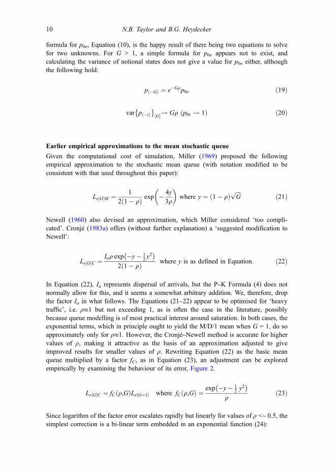
In Equation (22), Ia represents dispersal of arrivals, but the P–K Formula (4) does notnormally allow for this, and it seems a somewhat arbitrary addition. We, therefore, dropthe factor Ia in what follows. The Equations (21–22) appear to be optimised for ‘heavytraffic’, i.e. ρ≈1 but not exceeding 1, as is often the case in the literature, possiblybecause queue modelling is of most practical interest around saturation. In both cases, theexponential terms, which in principle ought to yield the M/D/1 mean when G = 1, do soapproximately only for ρ≈1. However, the Cronjé–Newell method is accurate for highervalues of ρ, making it attractive as the basis of an approximation adjusted to giveimproved results for smaller values of ρ. Rewriting Equation (22) as the basic meanqueue multiplied by a factor fC, as in Equation (23), an adjustment can be exploredempirically by examining the behaviour of its error, Figure 2.

Le G½ �C ¼ fC q,Gð ÞLe G¼1½ � where fC q,Gð Þ ¼ exp �y� 12 y

2� �

qð23Þ

Since logarithm of the factor error escalates rapidly but linearly for values of ρ <~ 0.5, thesimplest correction is a bi-linear term embedded in an exponential function (24):

10 N.B. Taylor and B.G. Heydecker

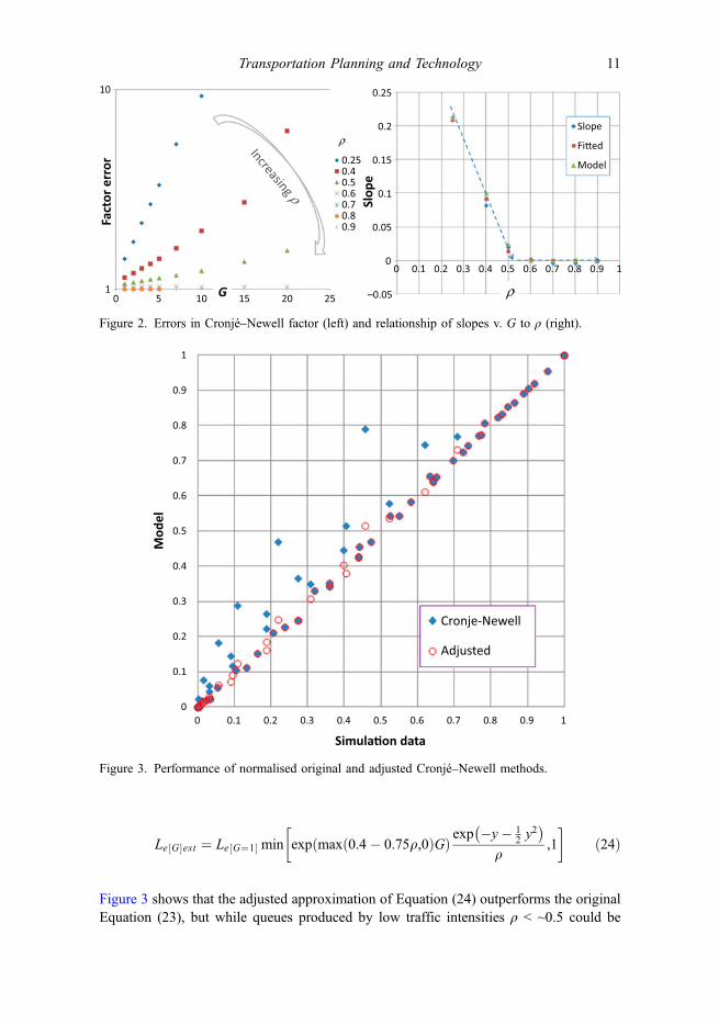
Le½G�est ¼ Le½G¼1� min exp max 0.4� 0.75q,0ð ÞGð Þ exp �y� 12 y

2� �

q,1

ð24Þ

Figure 3 shows that the adjusted approximation of Equation (24) outperforms the originalEquation (23), but while queues produced by low traffic intensities ρ < ~0.5 could be

Mod

el

1

0.9

0.8

0.7

0.6

0.5

0.4

0.3

0.2

0.1

00 0.1 0.2 0.3 0.4 0.5

Simula�on data0.6 0.7

Cronje-Newell

Adjusted

0.8 0.9 1

Figure 3. Performance of normalised original and adjusted Cronjé–Newell methods.

0.25

0.2

0.15

0.1

0.05

–0.05

00

Slope

Fi�ed

Model

0.1 0.2 0.3 0.4 0.5 0.6 0.7 0.8 0.9 1

Increasing r

0.25

r

r

0.40.50.60.70.80.9

01

10

5 10 15 20 25

Slop

e

Fact

or e

rror

G

Figure 2. Errors in Cronjé–Newell factor (left) and relationship of slopes v. G to ρ (right).

Transportation Planning and Technology 11

considered negligible for practical purposes, it is clear that some underlying structure hasnot been captured.

Link-function approach

The adjustment to Cronjé’s method in Equation (24) is unsatisfying because apart from itsone change of gradient, it conveys the message that no practical smooth function canrepresent the errors in a way that gives insight into an underlying structure.Experimentation reveals that the trends of p0e[G], Le[G] and Ve[G] for various values of ρand G can be made to overlap by transforming them using ‘link functions’ of the form ofEquations (25–26).

z hð Þ ¼ Gþ h

lsre qð Þ �Gþ h

sre1 qð Þ ð25Þ

where sre ¼ l�1 1� ffiffiffiq

p� ��2is a relaxation time. ð26Þ

For the sake of clarity, the dependence of z on ρ and G is, henceforth, ‘understood’. Thequantity τre is frequently cited as the stochastic relaxation time of a queue tendingtowards equilibrium. The variant τre1 = µτre is a dimensionless quantity which dependsonly on the demand intensity ρ. Hence the function z is also dimensionless and isindependent of µ.

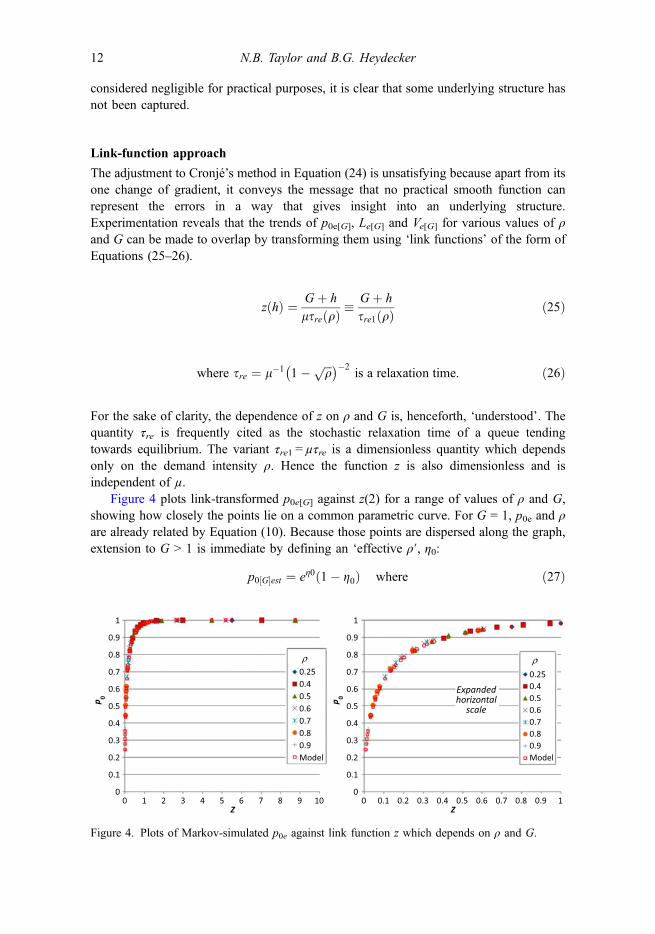
Figure 4 plots link-transformed p0e[G] against z(2) for a range of values of ρ and G,showing how closely the points lie on a common parametric curve. For G = 1, p0e and ρare already related by Equation (10). Because those points are dispersed along the graph,extension to G > 1 is immediate by defining an ‘effective ρ′, η0:

p0 G½ �est ¼ eg0 1� g0ð Þ where ð27Þ

1

0.9

0.8

0.7

0.6

0.5

0.4

0.3

0.2

0.1

00 1 2 3 4 5 6 7 8 9 10

p 0

1

0.9

0.8

0.7

0.6

0.5

0.4

0.3

0.2

0.1

010.90.80.70.60.50.40.3

Expandedhorizontal

scale

0.20.10

p 0

0.25

r

0.40.50.60.70.80.9Model

0.25

r

0.40.50.60.70.80.9Model

Z Z

Figure 4. Plots of Markov-simulated p0e against link function z which depends on ρ and G.

12 N.B. Taylor and B.G. Heydecker

g0 ¼ max 1�ffiffiffiffiffiffiffiffiffiffiffiffiGþ 2

3

r1� ffiffiffi

qp� �

,0

! !2

ð28Þ

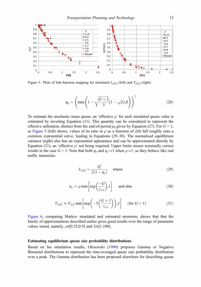
To estimate the stochastic mean queue, an ‘effective ρ′ for each simulated queue value isestimated by inverting Equation (11). This quantity can be considered to represent theeffective utilisation, distinct from the end-of-period p0 given by Equation (27). For G > 1,as Figure 5 (left) shows, values of its ratio to ρ as a function of z(0) fall roughly onto acommon exponential curve, leading to Equations (29–30). The normalised equilibriumvariance (right) also has an exponential appearance and can be approximated directly byEquation (31), an ‘effective ρ′ not being required. Upper limits ensure nominally correctresults in the case G = 1. Note that both η0 and η1→1 when ρ→1, so they behave like realtraffic intensities.

Le G½ � ¼ g212 1� g1ð Þ where ð29Þ

g1 ¼ qmin exp�G

sre1

� �,1

and also ð30Þ

Ve G½ � � Ve 1½ � min exp �3Gþ 1

sre1

� �� �,1

ðfor G> 1Þ ð31Þ

Figure 6, comparing Markov simulated and estimated moments, shows that that thefamily of approximations described earlier gives good results over the range of parametervalues tested, namely, ρ∊[0.25,0.9] and G∊[1,100].

Estimating equilibrium queue size probability distributions

Based on his simulation results, Olszewski (1990) proposes Gamma or NegativeBinomial distributions to represent the time-averaged queue size probability distributionover a peak. The Gamma distribution has been proposed elsewhere for describing queue

1

0.9

0.8

0.7

0.6

0.5

0.4

0.3

0.2

0.1

00 0.5 1 1.5 2 2.5

h/r

1

0.9

0.8

0.7

0.6

0.5

0.4

0.3

0.2

0.1

0

Vel/V

e(1)

0.25r

0.40.50.60.70.80.9Model

0.25r

0.40.50.60.70.80.9Model

Z (0)0 0.5 1 1.5 2 2.5

Z (1)

Figure 5. Plots of link-function mapping for simulated Le[G] (left) and Ve[G] (right).

Transportation Planning and Technology 13

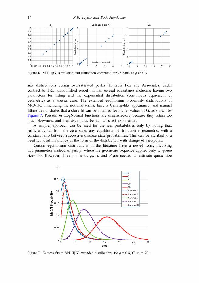
size distributions during oversaturated peaks (Halcrow Fox and Associates, undercontract to TRL, unpublished report). It has several advantages including having twoparameters for fitting and the exponential distribution (continuous equivalent ofgeometric) as a special case. The extended equilibrium probability distributions ofM/D/1[G], including the notional terms, have a Gamma-like appearance, and manualfitting demonstrates that a close fit can be obtained for higher values of G, as shown byFigure 7. Poisson or LogNormal functions are unsatisfactory because they retain toomuch skewness, and their asymptotic behaviour is not exponential.

A simpler approach can be used for the real probabilities only by noting that,sufficiently far from the zero state, any equilibrium distribution is geometric, with aconstant ratio between successive discrete state probabilities. This can be ascribed to aneed for local invariance of the form of the distribution with change of viewpoint.

Certain equilibrium distributions in the literature have a nested form, involvingtwo parameters instead of just ρ, where the geometric sequence applies only to queuesizes >0. However, three moments, p0, L and V are needed to estimate queue size

1

0.9

0.8

0.7

0.6

0.5

Mod

el e

stim

ated

Mod

el e

stim

ated

0.4

0.3

0.2

0.1

0

5

4

3

2

1

0

25

20

15

10

5

025201510505432

Markov simulated

1010.90.80.70.60.50.40.30.20.10

p0

Le (based on η) Ve

Figure 6. M/D/1[G] simulation and estimation compared for 25 pairs of ρ and G.

0.3

1251020Gamma 1Gamma 2Gamma 5Gamma 10Gamma 20

0.25

0.2

0.15

M/D

/1 P

roba

bilit

y

i+G

0.1

0.05

00 5 10 15 20 25 30

Figure 7. Gamma fits to M/D/1[G] extended distributions for ρ = 0.8, G up to 20.

14 N.B. Taylor and B.G. Heydecker

probability distributions (Taylor 2005), and three parameters are required to fit threeknown moments. With three parameters as in Equation (32), the distribution becomesdoubly nested geometric, whose first and second moments are given by Equation (33):

p0e ¼ 1� q� p1 ¼ q� 1� q̂ð Þ pi ¼ q�q̂ 1�~qð Þ~qi�2 ði � 2Þ ð32Þ

Le ¼ q� 1þ q̂�~qð Þ1�~q

Ve þ L2e ¼q� 1þ 3q̂�~q 2þ q̂�~qð Þð Þ

1�~qð Þ2 ð33Þ

By inverting the moments in Equation (33), the ‘effective ρs’ are obtained asEquations (34):

q� ¼ 1� p0e q̂ ¼ Ve þ Le Le � 1ð Þð Þ 1�~qð Þ22q�

~q ¼ Ve þ Le Le � 3ð Þ þ 2q�

Ve þ Le Le � 1ð Þ ð34Þ

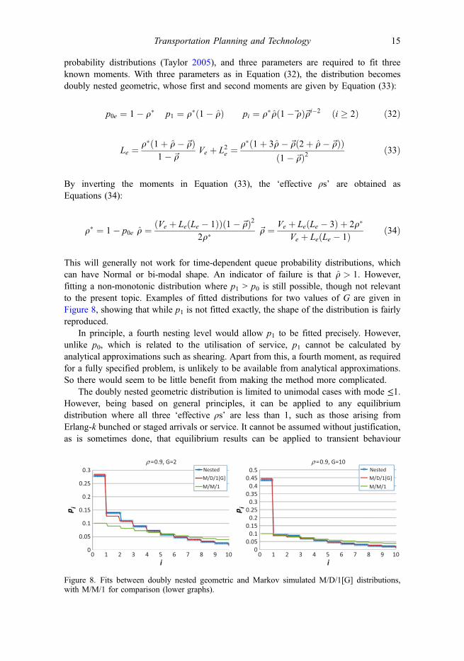
This will generally not work for time-dependent queue probability distributions, whichcan have Normal or bi-modal shape. An indicator of failure is that q̂ > 1. However,fitting a non-monotonic distribution where p1 > p0 is still possible, though not relevantto the present topic. Examples of fitted distributions for two values of G are given inFigure 8, showing that while p1 is not fitted exactly, the shape of the distribution is fairlyreproduced.

In principle, a fourth nesting level would allow p1 to be fitted precisely. However,unlike p0, which is related to the utilisation of service, p1 cannot be calculated byanalytical approximations such as shearing. Apart from this, a fourth moment, as requiredfor a fully specified problem, is unlikely to be available from analytical approximations.So there would seem to be little benefit from making the method more complicated.

The doubly nested geometric distribution is limited to unimodal cases with mode ≤1.However, being based on general principles, it can be applied to any equilibriumdistribution where all three ‘effective ρs’ are less than 1, such as those arising fromErlang-k bunched or staged arrivals or service. It cannot be assumed without justification,as is sometimes done, that equilibrium results can be applied to transient behaviour

00

0.05

0.1

0.15

0.2

0.25

0.3r =0.9, G=10r =0.9, G=2

0.5Nested

M/D/1[G]

M/M/1

Nested

M/D/1[G]

M/M/1

0.450.4

0.350.3

0.250.2

0.150.1

0.050

1 2 3 4 5i

6 7 8 9 10 0 1 2 3 4 5i

6 7 8 9 10

p i p i

Figure 8. Fits between doubly nested geometric and Markov simulated M/D/1[G] distributions,with M/M/1 for comparison (lower graphs).

Transportation Planning and Technology 15

(Sharma 1990). One of us (Taylor) has also been investigating ways of fitting functionsrepresenting instantaneous probability distributions to dynamic queue moments.

Discussion

No new work has been found relevant to the topic of the effect of green period capacityon signal queues since the derivation by Heidemann (1994), possibly because theproblem has been considered solved or of limited practical importance compared to theeffects of optimisation, adaptive timing, platooning, coordination, etc. State-of-the-artreviews by Rouphail, Tarko, and Li (1996) and Akçelik (1998) quote Newell’sapproximation, and the empirically corrected HCM and Australian formulae developedin the 1980s, but do not propose any new methods, possibly because existing ones areconsidered sufficient.

While acknowledging this, the motivation for this paper lies in widening the range ofqueue types that can be handled by computationally efficient time-dependent methodslike shearing, and in predicting variance and probability distributions along with means.That the green period effect emerges naturally from Heidemann’s derivation indicates thatit is more than just a convenient idealisation. Given that M/D/1 is taken to be a model of astochastic signal queue, it would seem remiss to ignore the effect of something soessential.

Aside from computational efficiency, the need for simplifying approximations inqueue calculation arises from the difficulty of describing even the simplest queueprocesses. Morse (1958) gives an exact formula for the time development of probabilitiesof the simplest M/M/1 random queue as a potentially infinite series of exponential orBessel functions. Even this only describes development from a precise initial size. Inrealistic calculations, convolution with an initial probability distribution is required.Kleinrock (1975) calls this situation ‘disheartening. While common methods exist foranalysing queuing, such as the P–K transform approach (e.g. Kleinrock 1975), recentresearch tends to be microscopic and complex (e.g. Mirchandani and Zou 2007).

A feature of queuing, as of nature generally, is that simple relationships may emergefrom a complex process through general principles of conservation and symmetry.Equilibrium results like that in Equation (4) are ‘emergent’ in the sense that exactformulae need not exist for the equilibrium mean of a general queuing process, since it isthe limiting outcome of an infinite sequence of random events repeated infinitely manytimes. Yet all queue processes must obey deterministic conservation Equation (3), which,therefore, cannot say anything about any result that depends on the details of the process.

An equilibrium queue is defined only for traffic intensities 0≤ ρ < 1 and is unboundedas ρ → 1. Thus it should be possible to normalise equilibrium moments by factoring byfinite expressions in ρ and G since this maps an infinite range into an infinite range. Aphysical interpretation is that random arrivals in green periods of different durationshould on average have a similar impact on the stochastic queue at the end of a period,provided that the relationship between green time and the characteristic stochastic timescale is the same. The link-function approach exploits this symmetry. But constant factorsare not necessarily appropriate for time-dependent queues. Expressing results in terms ofgeneric formulae (3) and (4) with modified parameters – in the present case ‘effective ρs’– allows the use of existing computationally efficient time-dependent methods.

On what basis can it be claimed that ‘effective ρs’ can be substituted directly into thetime-dependent methods? Physically, the longer the green period, the more traffic can

16 N.B. Taylor and B.G. Heydecker

‘disappear without trace’ before the queue is assessed at the end of the green period. Thistranslates into a reduction in the effective demand intensity and degree of saturation,which are the critical variables in time-dependent queuing. The quasi-static principlerelies on the rate at which information propagates through a queue being much greaterthan the rate of change of the queue itself so that the static relationship between queuesize and degree of saturation can be assumed to apply approximately to dynamic cases.As long as these assumptions hold, it should be possible to apply methods like shearingwith some confidence. Some observational validation of shearing was done by Kimberand Daly (1986). Validation of the extensions proposed here is part of a larger questionconcerning time-dependent methods, which involves considering dynamic probabilitydistributions or at least their moments, currently being addressed by one of us (e.g.Taylor 2005).

The primary impact of the work described here is, therefore, greater consistency. Theextent to which approximate time-dependent methods can accommodate realistic factorssuch as platooning, coordination and finite capacity queues has yet to be determined,though pursuance of research may depend on whether macroscopic modelling isconsidered likely to have a role as against microscopic simulation, an issue which isstill disputed (Wood 2012). An ad hoc method of accounting for green waves was used inCONTRAM (Taylor 2003), but manipulation of parameters in an extended P–K meanformula representing arrival and service statistics would be preferable. On the other hand,a purely statistical model like the P–K formula may be inappropriate to cases wherevariability of demand is no longer simply random (Chow 2013). Whether efficient time-dependent methods can continue to absorb real-life complexities through the imple-mentation of general principles may be a question for further research.

Conclusion

This paper responds to a perceived need to: (1) broaden the range of queue processes thatcan be modelled using computationally efficient time-dependent methods based on closedformulae; (2) incorporate variance and in particular (3) take account of the observationthat the size of a stochastic signal queue depends on the green period capacity and notjust the ratio of green to cycle time through the demand intensity.

An idealised stochastic signal queue process that takes account of green periodcapacity has been formulated by extending the basic M/D/1 model embodied in someexisting signal queue formulae. Simulation using Markov methods has been used togenerate test cases to compare with existing empirical approximations and to verify novelformulae for equilibrium values of the probability of zero queue, mean queue andvariance in a form compatible with computationally efficient macroscopic time-dependentmethods.

It is thought on structural grounds that the realism of transient behaviour using time-dependent methods should be similar to that for the basic process. Three moments enableprobability distributions to be estimated and a simple doubly nested geometricapproximation has been defined and demonstrated.

AcknowledgementsThe work described in this paper forms part of the first author’s research towards Ph.D. under thesupervision of the second author. An early version of the paper was presented at the UniversitiesTransport Studies Group (UTSG) Conference at Oxford, January 2013. Helpful comments by the

Transportation Planning and Technology 17

editors and two anonymous reviewers and the general support of Dr Alan Stevens TransportationChief Scientist at TRL are gratefully acknowledged.

Notes1. Strictly, capacity in vehicles should vary with traffic composition.2. G as used here corresponds to Olszewski’s B.3. We were unable to obtain permission to reproduce this, but some points taken from it are shown

in Figure 1 later.4. Some authors make C include the dispersion of arrivals also, but this does not emerge from the

derivation.5. The Markov simulation program used, which evaluates recurrence relations using small time

steps, was developed by the first author with algorithm design and programming assistance byNeil H Spencer, then a sandwich student at TRL.

ReferencesAkçelik, R. 1998. Traffic Signals: Capacity and Timing Analysis. Report ARR 123. Vermont South:

Australian Road Research Board. [Most recent edition of review first published 1981].Allsop, R. E., and T. P. Hutchinson. 1972. “Delay at Fixed-Time Traffic Signals [Parts I and II

Respectively].” Transportation Science 6 (3): 260–305. doi:10.1287/trsc.6.3.260.Burrow, I. J. 1987. OSCADY: A Computer Program to Model Capacities, Queue and Delays at

Isolated Traffic Signal Junctions. TRL Report RR 105. Crowthorne House: Transport ResearchLaboratory.

Chow, J. Y. J. 2013. “On Observable Chaotic Maps for Queueing Analysis.” In Proceedings of92nd TRB Annual Meeting, January 2013, January 13–17. Washington, DC: TransportationResearch Board.

Cronjé, W. B. 1983a. “Analysis of Existing Formulas for Delay, Overflow and Stops.”Transportation Research Record 905: 89–93. Washington, DC: Transportation Research Board.

Cronjé, W. B. 1983b. “Optimization Model for Isolated Signalized Traffic Intersections.”Transportation Research Record 905, 80–82. Washington, DC: Transportation Research Board.

Han, B. 1996. “A New Comprehensive Sheared Delay Formula for Traffic Signal Optimisation.”Transportation Research A 30 (2): 155–171.

Heidemann, D. 1994. “Queue Length and Delay Distributions at Traffic Signals.” TransportationResearch 24B (5): 377–389.

Kendall, D. G. 1951. “Some Problems in the Theory of Queues.” Journal of Royal StatisticalSociety B (Methodological) 13(2): 151–183.

Kimber, R. M., and P. Daly. 1986. “Time-Dependent Queuing at Road Junctions: Observation andPrediction.” Transportation Research 20B (3): 187–203.

Kimber, R. M., and E. M. Hollis. 1979. Traffic Queues and Delays at Road Junctions. TRL ReportLR 909. Crowthorne House: Transport Research Laboratory.

Kleinrock, L. 1975. Queueing Systems: Vol. 1 Theory. New York: Wiley Interscience.Meissl, P. 1963. “Zufallsmodell einer Lichtsignalanlage mit mehrspurigem Stauraum [A Random

Model of a Traffic Signal with Multilane Storage].” Mathematik-Technik-Wirtschaft 63 (1): 1–4and 63 (2): 63–68.

Miller, A. J. 1969. Some Operating Characteristics of Fixed-Time Signals with Random Arrivals.Sydney: Institution of Highways and Traffic Research, University of New South Wales.

Mirchandani, P. B., and N. Zou. 2007. “Queuing Models for Analysis of Adaptive Signal Control.”IEEE Transactions on Intelligent Transportation Systems 8 (1): 50–59. doi:10.1109/TITS.2006.888619.

Morse, P. M. 1958. Queues Inventories and Maintenance. New York: John Wiley.Newell, G. F. 1960. “Queues for a Fixed-Cycle Traffic Light.” Annals of Mathematical Statistics

31: 589–597. doi:10.1214/aoms/1177705787.Newell, G. F. 1965. “Approximation Methods for Queues with Application to the Fixed-Cycle

Traffic Light.” SIAM Review 7: 223–240. doi:10.1137/1007038.Olszewski, P. S. 1990. “Modelling of Queue Probability Distribution at Traffic Signals.” In

Proceedings of the International Symposium of Traffic and Transportation Theory, edited byM. Koshi, 569–588. New York: Elsevier.

18 N.B. Taylor and B.G. Heydecker

Rouphail, N., A. Tarko, and J. Li. 1996. “Traffic Flow at Signalized Intersections.” In Chapter 9 ofTraffic Flow Monograph. Washington, DC: Transportation Research Board, pp. 9-1–9-32. http://www.fhwa.dot.gov/publications/research/operations/tft/chap9.pdf

Sharma, O. P. 1990. Markovian Queues. Chichester: Ellis Horwood.Taylor, N. B. 2003. “The CONTRAM Dynamic Traffic Assignment Model.” Networks and Spatial

Economics Journal – Special Issue on Dynamic Traffic Assignment 3: 297–322. doi:10.1023/A:1025394201651.

Taylor, N. B. 2005. “Variance and Accuracy of the Sheared Queue Model.” In Proceedings of IMAMathematics in Transport Conference, edited by B. G. Heydecker, 259–278. Amsterdam:University College London, September 7–9.

Webster, F. V, and B. M. Cobbe. 1966. “Traffic Signals.” Road Research Technical Paper 56.London: HMSO.

Wood, S. 2012. “Traffic Microsimulation – Dispelling the Myths.” Traffic Engineering and Control53 (9): 339–344.

Transportation Planning and Technology 19