The Effect of Health on Earnings: Quasi-Experimental Evidence from Commuting Accidents

by

Martin HALLA*)

Martina ZWEIMÜLLER

Working Paper No. 1104 June 2011

DDEEPPAARRTTMMEENNTT OOFF EECCOONNOOMMIICCSS

JJOOHHAANNNNEESS KKEEPPLLEERR UUNNIIVVEERRSSIITTYY OOFF

LLIINNZZ

Johannes Kepler University of Linz Department of Economics

Altenberger Strasse 69 A-4040 Linz - Auhof, Austria

www.econ.jku.at

martin.halla@jku.at phone +43 (0)70 2468 -8706, -28706 (fax)

The Effect of Health on Earnings: Quasi-Experimental

Evidence from Commuting Accidents∗

Martin Halla Martina Zweimuller

University of Linz & IZA University of Linz

forthcoming in Labour Economics

(Last update: February, 2013)

Abstract

This paper interprets accidents occurring on the way to and from work as negative healthshocks to identify the causal effect of health on labor market outcomes. We argue that inour sample of exactly matched injured and non-injured workers, these health shocks (predomi-nantly impairments in the musculoskeletal system) are quasi-randomly assigned. A fixed-effectsdifference-in-differences approach estimates a negative and persistent effect on subsequent em-ployment and earnings. After initial periods with a higher incidence of sick leave, injuredworkers are more likely to be unemployed, and a growing share of them leave the labor marketvia disability retirement. Injured workers who manage to stay in employment incur persistentearnings losses. The effects are somewhat stronger for sub-groups of workers who are typicallyless attached to the labor market.

JEL Classification: I10, J22, D31, J31, J24, J26, J64, J28.Keywords: Health, employment, earnings.

∗Corresponding author: Martin Halla, Johannes Kepler University of Linz, Department of Economics, Altenberg-erstr. 69, 4040 Linz, ph.: +43 70 2468 8706, fax: +43 70 2468 28706, email: martin.halla@jku.at. For helpful commentswe would like to thank two anonymous referees and the Editor Bas van der Klaauw. The paper has also benefitedfrom comments and discussions with David Card, Emilia Del Bono, Carlos Dobkin, Marco Francesconi, NicolasZiebarth, Gerald Pruckner, Eddy van Doorslaer, Andrea Weber, Rudolf Winter-Ebmer, Josef Zweimuller, as well asfrom participants at the Annual Meeting 2010 of the Austrian Economic Association in Vienna, at the 2010 Con-ference of Applied Econometrics Association (Econometrics of Healthy Human Resources) in Rome, at the AnnualConference 2010 of the European Society for Population Economics in Essen, at the 2010 Congress of the EuropeanEconomic Association in Glasgow, and at the Research Seminar at the University of Innsbruck. The usual disclaimerapplies. Moreover, we thank the following institutions for providing us with data: Austrian Workers’ CompensationBoard, Central Institute for Meteorology and Geodynamics, Main Association of Austrian Social Security Institu-tions, Upper Austrian Health Insurance Fund, and the Austrian Federal Ministry of Finance. This paper was partlywritten during Martin Halla’s visiting scholarship at the Center for Labor Economics at the University of Californiaat Berkeley. He would like to express his appreciation for the stimulating academic environment at the center and thehospitality he received. This research was funded by the Austrian Science Fund (FWF): National Research NetworkS103, The Austrian Center for Labor Economics and the Analysis of the Welfare State.

1 Introduction

A positive correlation between health and socio-economic status is well documented in social and

medical sciences.1 However, a considerable debate about the causal underpinnings of this rela-

tionship remains. The identification of causal effects has proven to be extremely difficult (Deaton

and Paxson, 1998; Goldman, 2001; Fuchs, 2004). Due to the nature of the problem randomized

experiments are mostly not feasible and/or not appropriate. Thus, scholars have to rely on natural

experiments in order to identify causal effects.2 A small number of papers have managed to estab-

lish a causal effect of income on health.3 In sum, these papers (all studying data from developed

countries) find positive but quantitatively small effects of income on (mental) health.

An even smaller number of papers explore the causal effect of health on income. It seems

even harder to find and to measure arguably exogenous variation in health compared to income.

Wu (2003) argues that severe health conditions—such as strokes, cancer or diabetes—can be

interpreted as exogenous health shocks. In a similar vein, Riphahn (1999) defines a negative health

shock as a sudden and substantial drop in subjective health, Wagstaff (2007) uses a substantial drop

in the body mass index, and Garcıa-Gomez et al. (2011) exploit acute hospitalizations. However,

there are some doubts regarding the exogeneity of such events. For instance, Charles (2003)

analyzes the dynamic effects of a disability on earnings and finds that earnings have already dropped

one year before the onset of the disability. A different approach is given by accidents. Reville and

Schoeni (2001) and Crichton, Stillman and Hyslop (2011) study the effects of workplace (and non-

workplace) accidents on employment and income, and Møller Danø (2005) estimates the effect of

severe road accidents on labor market outcomes and public transfers.4 The evidence presented

in these papers is somewhat mixed, which may be explained by varying types of accidents used;

however, shows by and large negative effects of accidents on subsequent labor market outcomes.

In this paper, we follow a similar approach; however, we focus on a special type of accident.

We interpret accidents occurring on the way to and from work (such as road accidents, slip and

fall accidents and injuries due to falling objects) as negative health shocks. This has a number of

attractive features: (i) the way to and from work is part of the daily routine of every employed

individual and is (in contrast to general road accidents) not affected by leisure time activities, (ii)

the likelihood of such a commuting accident is (as compared to a workplace accident) not related

to self-selection into certain jobs, offering compensating wage differentials for hazardous workplace

environments, (iii) due to an institutional detail of the Austrian mandatory social accident insur-

ance we can observe the universe of commuting accidents in Austria, and link these to the Austrian

Social Security Database, a linked employer-employee data-set.

Still, there are some determinants of the likelihood of a commuting accident that may also affect

labor market outcomes. Preferences for working at (or close) to home, for living in an urban or

rural area, or for certain means of transportation for the work commute (such as train or bike) may

1For a review of this literature, see, for instance, Strauss and Thomas (1998); Smith (1999).2A notable exception of an experimental setting is given by Thomas et al. (2006).3On an individual-level scholars exploit exogenous variation in income due to inheritances (Meer, Miller and

Rosen, 2003), lottery winnings (Lindahl, 2005; Gardner and Oswald, 2007; Apouey and Clark, 2010) and the Germanreunification (Frijters, Haisken-DeNew and Shields, 2005). Based on cohort data Adda, Banks and von Gaudecker(2009) use changes in income mainly related to changes in the macro-economic environment. The identification ofMichaud and van Soest (2008) comes from dynamic linear panel data techniques.

4Relatedly, Lindeboom, Llena-Nozal and van der Klaauw (2007) use accidents of any type (reported by surveyrespondents) as an instrument for disability status to study the effect of a disability on employment.

2

affect selection into certain jobs. Some of these potential confounding factors are observable in our

data. For instance, given an additional link to data from the tax register we observe the commuting

distance for each individual. In order to account for remaining unobserved heterogeneity we follow

Heckman, Ichimura and Todd (1997)—who have shown that in the presence of longitudinal data,

matching and differencing can be fruitfully combined to weaken the underlying assumptions of

both methods—and compile a sample of matched treated and control individuals, who share an

observationally identical (labor market) history. Thanks to our rich data—before and after the

treatment—we can address the usual concerns about this approach. Most importantly, we find

strong evidence for a common trend in pre-treatment labor market outcome across injured and

non-injured units (common trend assumption). Based on data from a mandatory health insurance,

we can further show that the two groups have been following the same trends in objective health

outcomes before the treatment. We argue that within our research design commuting accidents

are quasi-randomly assigned, and constitute negative health shocks that enable us to establish a

causal effect of health on employment and labor market income (henceforth earnings).

Which type of health shocks do commuting accidents generate? While we have no information

on the type of injuries in our individual level data, we can resort to aggregate statistics.5 These

show a wide range of injuries: head and neck (31 percent), trunk (16 percent), upper limbs (11

percent) and lower limbs (18 percent), potentially accompanied by mental stress. That means, our

health shocks are predominantly impairments in the musculoskeletal system. Clearly, our research

design does not allow us to infer on the effects of typical lifestyle diseases, such as cardiovascular

diseases, strokes or cancer. However, it is hard to think of exogenous variation in the incidence of

these lifestyle diseases.

Our estimation results show that negative health shocks (i. e., predominantly impairments in

the musculoskeletal system) that result in an initial average sick leave spell of 46 days, reduce the

likelihood of subsequent employment persistently. Five years after the commuting accident, injured

workers are still about four percentage points less likely to be employed. Initially the accident

increases the likelihood of sick leave, then injured workers are more likely to be unemployed, and

over time a growing share of them leave the labor market via disability retirement. The injured

workers who manage to stay in employment experience persistent earnings losses of about minus

two percent. The size of the estimated effects varies along the dimensions of sex, occupation,

and age. Employment effects are strongest for female, older and blue-collar workers. The highest

earnings losses (up to minus three percent) are observed for young workers. While we do not

observe much adapting behavior of injured workers in terms of job mobility, we find evidence that

injured female workers adjust their fertility behavior in response to the negative health shock.

The remainder of the paper is organized as follows: First, we discuss our research design and

outline relevant institutional facts. This section also describes the data and provides descriptive

statistics for our estimation samples. The next two sections explain our estimation strategy and

discuss the identifying assumption. Subsequently, we present our estimation results for all workers

and explore heterogenous treatment effects along the dimensions of sex, occupation and age. We

also examine potential adapting behavior and provide a discussion on the channels through which

injured individuals leave the labor market. The final section summarizes and concludes the paper.

5Note, aggregate injury statistics are only available for accidents with subsequent hospitalization and do notdistinguish between commuting accidents and all other road accidents. Source: Kuratorium fur Verkehrssicherheit.Freizeitunfallstatistik 2007.

3

2 Research design

In Austria, a social accident insurance is mandatory for every employed individual, student and

pupil. The Austrian Workers’ Compensation Board (AWCB) is the major social accident insurance

institution and covers about 76.2 percent of all insurance holders.6 In 2007, the AWCB provided

insurance for more than 3.2 million employed individuals, 1.4 million self-employed and 1.3 million

students and pupils. Employers have to pay 1.4 percent of the total wage bill to the AWCB, which

amounted to 1.1 billion Euro in 2007 (Source: Handbuch der Osterreichischen Sozialversicherung

2008 ). The social accident insurance covers occupational accidents and occupational diseases.

Occupational accidents are unexpected external events causing injury, in locational, temporal and

causal relationship to the insurant’s occupation or education. Occupational diseases are health

impairments caused by the insurant’s occupation or education and are explicitly listed in the

annex to the General Social Insurance Act. Employers (and educational authorities) are bound by

law to report every occupational accident and disease to the respective social accident insurance

institution. Workers who are disabled as a consequence of an occupational accident (or disease),

are eligible for a lifelong disability compensation; which is equal to about two thirds of the earnings

in the preceding year (subject to a cap). Partly disabled insurants receive a reduced (pro rata)

compensation.

We exploit the fact that accidents occurring on the way between the place of residence and

the place of work (or education) are also classified as occupational accidents. We interpret these

commuting accidents as negative health shocks and argue that in a sample of exactly matched

treated and control workers, this special type of accident is quasi-randomly assigned.7 To construct

our estimation sample we start with the AWCB Database and retrieve detailed information on all

workers who had a commuting accident that occurred between January 1, 2000 and December 31,

2002 and resulted in at least one day of sick leave (treated individuals). In the case workers had two

or more commuting accidents during this treatment period, we only consider the first accident as

our treatment, since all following accidents may be causally affected by the first incident. Further,

we exclude all workers from the analysis who died in the quarter of the accident.8 All workers who

had no commuting accident during that period serve as potential control units.

The Austrian Social Security Database (ASSD) allows us to follow the treated and the con-

trol individuals before, during and after the treatment period (until December 31, 2007). We

observe their labor market status in employment (including basic employer information), unem-

ployment, and various other qualifications on a daily basis. The ASSD collects detailed information

on all workers in Austria. Since the ASSD is an administrative record to verify pension claims

the information is very precise. Information on earnings is provided per year and per employer.

The limitations of the data are top-coded wages and the lack of information on working hours

(Zweimuller, Winter-Ebmer, Lalive, Kuhn, Wuellrich, Ruf and Buchi, 2009). In combination with

the database from the Austrian Federal Ministry of Finance we can compute each individual’s

6Beside the AWCB three other social accident insurance institutions are responsible for special types of self-employed and employees (and their dependants).

7Accidents that occur to workers who are customarily and regularly engaged away from the employer’s place ofbusiness (e. g. outside sales workers or taxi drivers) are not counted as commuting accidents, except they occurbetween the place of residence and the central office.

8Workers who died later are included until their quarter of death. In our sample, 1.27 percent of treated workersand 1.26 percent of control workers die in the post-treatment period.

4

commuting distance in kilometers based on the zip code of her place of work and her place of

residence. Moreover, the latter database allows us to obtain some information on working hours

(i. e. full-time versus part-time employment). TableA.1 in the Appendix A provides an overview

of all our data sources.

Our potential control group consists of all workers who have been employed (and insured with

the AWCB) at least once during the treatment period (otherwise they have not been at risk to

have a commuting accident) and had no commuting accident. In order to distinguish a pre- and

post-treatment period for our control units, we randomly assign a quarter between January 1,

2000 and December 31, 2002. If these workers have not been employed in their randomly assigned

quarter, we exclude them from our analysis, since information on employment in that quarter is

crucial for our matching procedure (see below). To generate a homogenous sample we only consider

individuals who were ‘regularly’ employed in the treatment quarter, i. e. we exclude workers in

marginal employment or dependent self-employment. Furthermore, we restrict our analysis to

individuals who were employed as either blue-collar or white-collar workers throughout the pre-

treatment period.9 Finally, to guarantee that we can (potentially) observe all individuals before

and after the treatment on the labor market we restrict our sample to individuals between 25 and

50 years of age at the time of the (potential) accident.

After applying these sample selection criteria we observe 1.682, 602 individuals without an

accident, and 11, 397 individuals with an accident that resulted at least in one day of sick leave.10

We use the length of the sick leave spell after the accident as a proxy for severity. This information

is documented in the AWCB database. The distribution of weeks on sick leave is shown in Figure 1.

On average, the sick leave spell lasts about four weeks. Half of the individuals spend at least two

weeks on sick leave. Clearly, the length of this sick leave spell is an imprecise measure for the

severity of the accident, since it might vary with worker’s motivation to return to work. This

problem is mitigated (at least to some degree) by the fact that sick leave spells longer than three

days are subject to medical verification. Moreover, we see in a sub-sample (described in Appendix

B) that the sick leave spell length (among the treated) has a very high correlation with health care

service utilization. Still, we use the length of the sick leave spell with care and distinguish only

between accidents below and above the median, to define individuals with less and more severe

accidents. In our main analysis we will concentrate on the sub-set of 5, 909 treated individuals with

more severe accidents.11 Most of these accidents (almost 65 percent) involve a vehicle. A significant

fraction (about 33 percent) is due to slip and fall (e. g. on stairs, ice, snow or slippery ground).

The remaining two percent of accidents include, among others, injuries due to falling objects

and crushing injuries. That means, the health shocks under consideration are predominantly

impairments in the musculoskeletal system.

9That means that we exclude civil servants, self-employed and farmers. This guarantees that we can observepre-treatment earnings for all individuals. The ASSD does not provide information on earnings of civil servants;earnings of self-employed and farmers are only recorded since 1997.

10About 5, 000 individuals had an accident but had zero days of sick leave. We exclude these individuals fromour analysis since they obviously had only a minor accident. In an additional estimation analysis, we exploit theidea that this group is not injured, but is supposedly quite comparable to our treatment group. Using them as analternative control group gives results that are very comparable to those in our main analysis.

11In order to check the sensitivity of this sample selection criteria we alternatively used hospitalization to splitthe sample. Clearly, the hospitalization decision is less discretionary than the amount of sick leave. The estimationresults have the same patterns across the two sample selection criteria (compare Table 2 and 3 with TableA.2 andA.3 in the Appendix A)—the employment effects are at a higher level in the latter case, since these are on averagemore severe accidents.

5

It should be noted that workers who had an accident during their leisure time have almost no

possibility or incentive to cheat and to falsely report that the accident took place on the way to

or from work. Employees have to report the accident to the employer without delay, and in case

the injured worker needs medical treatment the exact time and date is recorded by the doctor or

hospital. Furthermore, irrespective of whether the accident happened on the way to or from work

or in leisure time, the health care cost and the compensation for lost earnings caused by temporary

sickness are covered by an insurance in either case.12 This claim is supported by the distribution of

commuting accidents by weekday and daytime (see Figure 2). As expected, most of the accidents

take place Monday through Friday, and during rush hours.

Table 1 compares the average characteristics of treated and a random sample of control workers

in the quarter of the (potential) accident. Since we measure all characteristics on the first day of

each quarter, the quarter of the (potential) accident is the last quarter of the pre-treatment period.

The comparison of treated and control individuals (the first two columns) reveals that there are

some significant differences in the average characteristics of these two groups. Treated workers

have a longer commute (about plus four kilometers). This seems plausible; the longer the way to

work the higher the likelihood of a commuting accident. Further, treated individuals are slightly

older and more likely female.13 The most important difference is in the distribution of occupational

groups. The share of blue-collar (white-collar) workers is higher among the treated (control).14

Consequently, we find that treated individuals are less likely to have a degree, have somewhat lower

earnings, slightly less working experience, and a shorter tenure. A plausible explanation for the

higher incidence of commuting accidents among blue-collar workers are different work schedules.

Blue-collar workers are more likely to work in a shift system. That means, they have to commute

early in the morning or later at night. At these hours unfavorable lightening and road conditions

may promote accidents of any kind.15 In line with this supposition we see a clear pattern that

blue-collar workers accidents’ are more likely to happen very early in the morning or later at night

(see Figure 2 in the Appendix A). Further differences can be found with respect to the type of

employers. Treated individuals tend to work in larger firms and are more likely to be employed

in the manufacturing sector. This partly reflects an unequal distribution of blue- and white-collar

workers across employers, but also a correlation with the commuting distance. Larger firms (or

firms from certain industries) tend to be in peripheral enterprise zones, which implies a comparable

longer commute for their employees.

These descriptive statistics suggest that commuting accidents do not happen perfectly ran-

domly, hence we are concerned with selection that might complicate the comparison of treated and

12Depending on whether the accident is occupational or non-occupational, the health care cost are either coveredby the social accident insurance or the social health insurance. In both cases, the compensation for lost earnings (theso-called Entgeltfortzahlung) is initially (i. e. at least eight weeks) disbursed by the employer. After a certain lengthof sick leave this compensation is covered by the social accident insurance or the social health insurance, respectively.The only important difference is with respect to rehabilitation cost. In case of an occupational accident the socialaccident insurance may provide special occupational retraining and extra disability benefits.

13Notably, the sex distribution of commuting accidents is in stark contrast to that of any other type of accident. In2002 females accounted only for 20.6 percent of all workplace accidents, 40.9 percent of road accidents, 29.0 percentof sports accident and 45.2 percent of other leisure time accidents. Sources: Kuratorium fur Verkehrssicherheit(Unfallstatistik 2002); own calculations based on the AWCB Database.

14The distinction between blue- and white-collar workers follows the Austrian legal definition and is recorded inthe ASSD. Blue-collar workers typically perform manual labor and are directly involved in the production process.In contrast, white-collar workers are non-manual workers in supervising and administrative jobs.

15In fact it is documented that most of the pedestrian and vehicle occupant fatalities occur during the changefrom daylight to twilight or vice versa (Ferguson, Preusser, Lund, Zador and Ulmer, 1995).

6

control individuals. To correct for differences between these groups, we perform exact matching

based on their labor market history, and apply a DiD approach (based on samples stratified by

sex, occupation, and age). After describing our matching procedure and the resulting sample,

we will spell out our identifying assumption and discuss potential pitfalls. We will also provide

supplementary analyses that substantiate the validity of our identifying assumption.

3 Empirical strategy

In the empirical analysis we combine two identification strategies to uncover a causal effect of

negative health shocks on labor market outcomes. First, we use exact matching to establish the

pre-treatment comparability of the treatment and control group, and second, we apply a DiD

estimator on the sample of matched treated and control units. In the context of longitudinal data,

the combination of matching and DiD can accommodate (i) differences in observed characteristics,

and (ii) differences in unobserved characteristics as long as they are constant over time (Heckman

et al., 1997). The DiD approach requires a common trend assumption, which implies that in

absence of the negative health shock the average labor market outcomes of treated and control

workers follow parallel paths over time. Since we have data for a long time period before the

(potential) treatment we can check the series of average outcomes of the two groups.

Figure 3 shows the employment rate and the average daily wage (conditional on employment)

by treatment status. We normalize the quarter of the (potential) accident to zero and observe

each worker 20 quarters before and after the treatment. For both groups, the employment rate

increases rapidly up to the quarter of the (potential) treatment, when it becomes one, and decreases

thereafter. This pattern is a consequence of the fact that we select only workers who were employed

in this quarter. As these workers are also more likely to have been in employment in the periods

leading to the reference quarter, we observe an increasing (decreasing) employment rate in the

quarters preceding (subsequent to) the reference quarter. What is important to notice, is that we

observe a common trend in employment among treated and control prior to the quarter of the

(potential) treatment. This is clear evidence for a common underlying trend of treated and control

units. The observed drop in the employment rate after the (potential) treatment is first evidence

for an effect of the health shock on employment. An equivalent picture can be observed for the

average daily wage. When analyzing earnings we always restrict our sample to employment spells,

since positive earnings are observed only for employed workers.16 After the (potential) treatment,

we observe a slower wage growth path for treated workers, which is first evidence of a negative

effect of the health shock on earnings. Alternatively, FigureA.1 in the Appendix A provides a

regression-adjusted graphical depiction that removes the pattern caused by the selection rule.

On the basis of the full sample we perform exact matching of treated and control units. In

the quarter of the (potential) treatment individuals must have the same sex, age (13 age groups:

25−26, 27−28, . . . , 49−50), education (no academic degree, engineer, MA/MSc, PhD), region of

residence (West, East, South, abroad/missing), industry (agriculture, fishing, mining and energy;

manufacturing; construction; wholesale, retail and repair; transport and communication; services;

missing) and commuting distance (by quintile group plus additional groups for zero and missing

16Note, the drop in the average wage in the quarter of the (potential) accident is a consequence of the fact that werestrict our sample to employment spells when looking at wages. In the reference quarter, all workers—also thosewith the least earnings potential—are employed.

7

distance). On top of that, in the quarter of the treatment and in each of the three preceding

quarters their employment status (employed, not employed), broad occupation (blue-collar, white-

collar), and the log of the deflated daily wage rate (by decile groups plus an additional group for

non-employed individuals) must coincide. Further we use their quarter of (potential) treatment as

a matching criterion. Since some treated individuals may have more control subjects than others

we construct weights that compensate for differences in cell size.17

Applying this matching procedure we are able to find at least one control unit for 58 percent

of our treated individuals, i.e. our estimation sample consists of 3, 406 treated and 26, 734 control

units. Columns three and four of Table 1 provide descriptive statistics for the matched sample.

While treated and control workers should not differ in the matching variables (e. g. age, daily

wage, commuting distance), it is reassuring that differences in characteristics that were not among

the matching variables, for instance, experience and tenure, are only minor. The only exception is

with respect to firm size; matched treated workers are employed in larger firms than their control

counterparts.18 In order to see the impact of our matching procedure, one can compare Figure 3

(showing the average employment rate and earnings by treatment status in the full sample) with

the equivalent figure for the matched sample (see FigureA.2 in the Appendix A).

Based on this sample we estimate the impact of a negative health shock on labor market

outcomes (such as employment and earnings) up to five years after the treatment. To make sure

that we partial out potential remaining (un)observed heterogeneity we apply a DiD approach to

our sample of exactly matched treated and control units. We start with a simple DiD model:

outcomeit = α0 + α1Ti + α2Pt + α3Pt × Ti + βXi(t) + θt + ǫit, (1)

where i denotes workers and t denotes time measured in quarters running from −20 to 20. In a

first step we consider the two outcomes, employment and earnings. To capture employment we use

a binary variable equal to one if individual i is employed on the first day of the quarter t, and zero

otherwise. Earnings are measured by the log of the deflated daily wage rate. The binary variable

Ti is equal to one if individual i is treated and zero otherwise. The variable Pt captures the post-

treatment period. For simplicity, we pool in a first step all quarters in the pre-treatment period

and in the post-treatment period and use a binary variable instead of a full set of quarter dummies.

Further, we control for absolute (calendar) time-fixed effects θt (consecutive quarter dummies) and

a set of individual characteristics Xi(t) that comprises age-fixed effects and further characteristics

that are predetermined at the quarter of the (potential) treatment.19 The parameter of primary

interest is α3, which gives the estimated causal effect of the negative health shock.

In order to allow for varying effects of the negative health shock over time, we extend the model

17The weights for treated and controls are constructed as follows: treated have a weight of wi = 1 and controls

have a weight of wi =m

S

C

mS

T

·

mC

mT, where mT and mC are the total number of matched treated and controls, and mS

T

and mS

C are the number of treated and controls in cell S.18It can be noted that our estimation results are robust to using firm size as an additional matching criterion.

Detailed estimation output is available upon request.19We control for the following characteristics measured in the quarter of the accident: sex, education (no academic

degree, engineer, MA/MSc, PhD), citizenship (Austrian, non-Austrian), broad occupation (blue-collar, white-collar),place of residence (nine states), location of firm (nine states plus missing), commuting distance (by quintile groupplus additional groups for zero and missing distance), industry of the firm (agriculture, fishing, mining and energy;manufacturing; construction; wholesale, retail and repair; transport and communication; services), firm size (log ofthe number of employees), tenure (in years), work experience (in years), and the quarter of the (potential) accident.

8

in the following way

outcomeit = α0 + α1Ti +20∑

r=1

γrQr +20∑

r=1

δrQr× Ti + βXi(t) + θt + εit, (2)

where Qr denotes a series of binary variables equal to one if the treatment has been r quarters ago.

This dynamic model allows us to trace out the full dynamic response of employment and earnings to

the negative health shock, where the estimated causal effect r quarters after the treatment is given

by δr. We check the robustness of our results by including in both models individual fixed-effects

which account for unobserved time-invariant heterogeneity. In this case, the treatment indicator

Ti and all predetermined characteristics are dropped, and Xi(t) only comprises age dummies.

4 Identifying assumption

The main identifying assumption is that the potential labor market outcomes of treated and

controls are independent of the treatment status conditional on observed and time-invariant unob-

served characteristics, i. e. the remaining error term is not correlated with the probability to have

an accident and potential labor market outcomes.

Under which conditions would this assumption fail? A potential pitfall of our estimation

strategy is that a job-loss (or a drop in earnings) causes the accident and not vice versa. Fortunately,

we will see below that the effect of the accident on employment (and on earnings) kicks in only with

some lag. In other words, the timing of the events strongly rejects the case of reverse causality.

Another source of problems are unobserved confounding factors that vary over time. Put

differently, we have to ponder on a third factor that causally affects labor market outcomes and

that is also correlated with a higher accident probability. Obviously, there is a plethora of factors

promoting an accident. Assignment into treatment may result, for instance, from own inattention,

sleepiness, other careless traffic participants, bad weather or lightening conditions, as well as any

other form of distraction. Some of these factors are undoubtedly exogenous; a third party’s fault

or bad weather conditions should not be correlated with the treated individual’s subsequent labor

market outcomes. However, inattention or sleepiness might be the result of already existing health

problems or another drastic personal event that may independently affect labor market outcomes.

To be more specific, if (i) another drastic personal event (such as sickness, alcoholism, divorce,

or death in family) takes place at the same time, (ii) that is the (only) causal determinant of the

observed changes in labor market outcomes, and (iii) that is also causing (or at least correlated)

with the accident, our identifying assumption would fail, and we would erroneously conclude that

the negative health shock affects labor market outcomes. While a high incidence of such systematic

patterns (i. e. all three conditions are fulfilled) seems unlikely, we can not completely rule it out. To

substantiate our interpretation that the estimated effects are causally related to the negative health

shock, and not caused by any other unobserved personal event, we conduct three supplementary

analyses.

First, we look at the effects of the accident on different health outcomes, and compare them

with the estimated effects of the accident on labor market outcomes.20 The idea is that if the

20 Since data on health outcomes is only available for workers from Upper Austria this analysis is based on asub-sample of the data. Details on the data, which are derived from the database of the Upper Austrian Health

9

accident causally affects subsequent labor market outcomes, we should observe dynamic effects

of the accident on health outcomes that resemble the dynamic effects of the accident on labor

market outcomes over time. Figure 4 depicts the estimated effect of the accident on sick leave

for the 20 quarters after the accident, based on the dynamic model, which controls in addition

for leads starting at quarter minus 7. First it can be noted that the coefficients capturing the

quarters prior to the accident are individually and jointly statistically insignificant, quantitatively

very small (basically zero) and do not exhibit a trend. That means, the timing evidence clearly

suggests that the accident causally affects subsequent sick leave. On top of that it rules out that

any pre-treatment injury or (arising) illness has triggered the accident (which could also be a

potential confounding factor). As expected, in the quarter of the accident we find a huge spike;

treated workers are estimated to be 18.6 days (or 490 percent) more on sick leave. This positive

effect decreases thereafter, however, is still statistically significant different from zero until one year

after the accident. As we will see in detail below, these dynamic effects of the accident on sick

leave are perfectly compatible with the estimated effects of the accident on labor market outcomes.

The same patterns as in the case of sick leave, can be observed for other health outcomes, such

as the incidence of hospitalization and extramural health expenditures. (Details are provided in

Appendix B.) In sum, this analysis of health outcomes supports our causal interpretation. The

only potential pitfall left is given by an unobserved time-variant confounding factor that exhibits

dynamic effects on labor market outcomes that by coincidence resemble the effects of the accident

on health outcomes.

In order to provide evidence against the latter case, we look at the effect of less severe accidents.

If the accident is indeed the causal determinant of subsequent labor market outcomes, we expect

smaller treatment effects in the case of less severe accidents. Relating to the reasoning from

above, it seems highly unlikely that less and more severe accidents are consistently correlated with

unobserved time-variant confounding factors that have small and larger effects on labor market

outcomes (resembling by coincidence the dynamic effects of the accident on health outcomes). The

analysis (summarized in Appendix C) indeed shows that less severe accidents are estimated to

have less (or no) effects on labor market outcomes.

As a final check, we aim to show that accidents are caused by exogenous events. While it is hard

to measure all (or even one) factor, we managed at least to obtain information on local weather

and lightening conditions. The regression analysis summarized in Appendix D shows— in line with

existing literature (Qiu and Nixon, 2008)—that weather conditions are statistically significant

determinants of accidents. For instance, we find that on days with an above average precipitation

(i. e. compared to an historical average at this specific location on this specific calendar day) the

likelihood of an accident increases for women (men) by 4.4 (2.0) percentage points. This result

supports the idea that commuting accidents are driven by exogenous (or random) factors that

justify its interpretation as a negative health shock.21

Insurance Fund, are provided in Appendix B.21We also tried to exploit this exogenous variation in the likelihood of a commuting within an instrumental variable

framework. This approach gives qualitatively very similar results (compared to the results based on the estimationstrategy explained above), however, the estimated effects are larger in (in absolute terms) and the standard errorsincrease considerably. Given that the F-statistic on the excluded weather variable in the first stage of our two-stageleast square estimation is not sufficiently high (especially for males), we decided not to present these results in moredetail.

10

5 Estimation results

This section presents our estimation results in the following way: first, we discuss the findings

on the effects of an accident on employment and earnings for all workers. We find that such a

negative health shock deteriorates labor market outcomes along any dimension. In a next step,

we explore heterogeneous treatment effects across sex, occupation, and age. Then we examine

potential adapting behavior of treated workers in terms of job mobility across employers and

industries. Finally, we distinguish between different forms of non-employment and show to what

extent treated workers leave the labor market through unemployment, retirement and parental

leave.

5.1 Baseline results

We consistently find that individuals who have experienced a commuting accident are subsequently

less likely to be employed, and (conditional on being employed) earn lower wages. Based on our

exactly matched sample, the static employment model estimates that treated individuals are on

average 3.3 percentage points less likely to be employed in the twenty quarters after the accident.

Notably, the estimated coefficients of the OLS and the FE model (see first line in Table 2) are

basically identical. We interpret this as evidence that our research design is very clean and that

accidents on the way to and from work are exogenous in our context. Based on our full sample

we find somewhat larger employment effects (about minus 4.7 percentage points). However, again,

the inclusion of individual fixed effects has almost no impact on the estimated coefficients (see

TableA.4 in the Appendix A).

The estimation results of the dynamic employment model corroborate the findings of the static

model and reveal interesting patterns. The upper panel of Figure 5 shows that treated units are

(compared to control units) equally likely to be employed in the quarter of the accident. It seems

plausible that employers may hesitate to layoff workers during their sick leave, or more generally,

shortly after an accident. However, starting with quarter two after the accident a statistically

negative employment effect for treated units can be observed each quarter in the post-treatment

period. The timing of the accident and the employment effect provides strong evidence against

reverse causality. The largest effect (in absolute terms) can be observed in quarter two after the

accident (about minus 4.8 percentage points). Over the following twelve quarters the effect is stable

around minus 2.8 percentage points, and from quarter fifteen to twenty the effect is estimated to

decrease somewhat again. In sum, these results show that a negative health shock has persistent

effects on employment.

When we look at wage effects, we have to restrict our sample to employment spells. It is hard to

evaluate whether the resulting sample selection bias is relevant in size. However, it seems plausible

to assume that the treated workers who return to employment are positively selected in terms of

their willingness to perform. Given that our results discussed below would underestimate the true

effect of the negative health shock on wages in absolute terms, since we compare the positively

selected treated workers with the average (or unselected) control workers. When we interpret the

estimated effects on wages earnings, we further have to keep in mind that we only observe daily and

not hourly wages . Variation in daily wages may result from an effect of the accident on working

hours and/or the wage rate. While we have no information on the exact number of working hours,

11

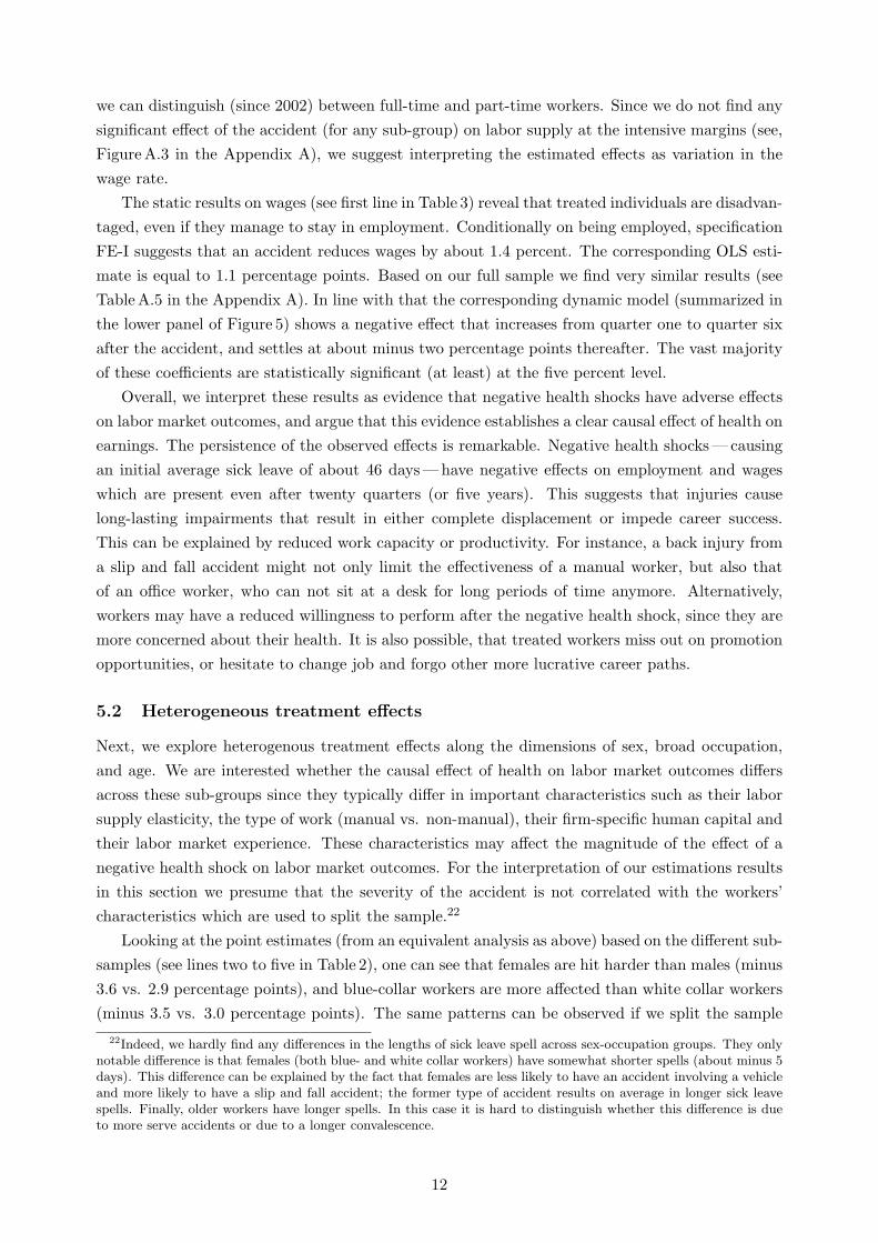
we can distinguish (since 2002) between full-time and part-time workers. Since we do not find any

significant effect of the accident (for any sub-group) on labor supply at the intensive margins (see,

FigureA.3 in the Appendix A), we suggest interpreting the estimated effects as variation in the

wage rate.

The static results on wages (see first line in Table 3) reveal that treated individuals are disadvan-

taged, even if they manage to stay in employment. Conditionally on being employed, specification

FE-I suggests that an accident reduces wages by about 1.4 percent. The corresponding OLS esti-

mate is equal to 1.1 percentage points. Based on our full sample we find very similar results (see

TableA.5 in the Appendix A). In line with that the corresponding dynamic model (summarized in

the lower panel of Figure 5) shows a negative effect that increases from quarter one to quarter six

after the accident, and settles at about minus two percentage points thereafter. The vast majority

of these coefficients are statistically significant (at least) at the five percent level.

Overall, we interpret these results as evidence that negative health shocks have adverse effects

on labor market outcomes, and argue that this evidence establishes a clear causal effect of health on

earnings. The persistence of the observed effects is remarkable. Negative health shocks—causing

an initial average sick leave of about 46 days—have negative effects on employment and wages

which are present even after twenty quarters (or five years). This suggests that injuries cause

long-lasting impairments that result in either complete displacement or impede career success.

This can be explained by reduced work capacity or productivity. For instance, a back injury from

a slip and fall accident might not only limit the effectiveness of a manual worker, but also that

of an office worker, who can not sit at a desk for long periods of time anymore. Alternatively,

workers may have a reduced willingness to perform after the negative health shock, since they are

more concerned about their health. It is also possible, that treated workers miss out on promotion

opportunities, or hesitate to change job and forgo other more lucrative career paths.

5.2 Heterogeneous treatment effects

Next, we explore heterogenous treatment effects along the dimensions of sex, broad occupation,

and age. We are interested whether the causal effect of health on labor market outcomes differs

across these sub-groups since they typically differ in important characteristics such as their labor

supply elasticity, the type of work (manual vs. non-manual), their firm-specific human capital and

their labor market experience. These characteristics may affect the magnitude of the effect of a

negative health shock on labor market outcomes. For the interpretation of our estimations results

in this section we presume that the severity of the accident is not correlated with the workers’

characteristics which are used to split the sample.22

Looking at the point estimates (from an equivalent analysis as above) based on the different sub-

samples (see lines two to five in Table 2), one can see that females are hit harder than males (minus

3.6 vs. 2.9 percentage points), and blue-collar workers are more affected than white collar workers

(minus 3.5 vs. 3.0 percentage points). The same patterns can be observed if we split the sample

22Indeed, we hardly find any differences in the lengths of sick leave spell across sex-occupation groups. They onlynotable difference is that females (both blue- and white collar workers) have somewhat shorter spells (about minus 5days). This difference can be explained by the fact that females are less likely to have an accident involving a vehicleand more likely to have a slip and fall accident; the former type of accident results on average in longer sick leavespells. Finally, older workers have longer spells. In this case it is hard to distinguish whether this difference is dueto more serve accidents or due to a longer convalescence.

12

by both, occupation and sex (see lines six to nine in Table 2). Female blue-collar workers suffer the

most (minus 3.9 percentage points), and male white-collar workers are affected least (minus 2.1

percentage points). Although the differences are not statically significant at conventional levels,

this is suggestive evidence that sub-groups which are typically less attached to the labor market

(i. e. females23), or have on average more unemployment spells (i. e. blue-collar workers), have also

a higher likelihood to withdraw from employment as a consequence of a negative health shock. This

can be explained by a higher lay-off probability (after a negative health shock); blue-collar workers

and part-time workers have less firm-specific human capital and can be substituted more easily.

Alternatively, factors that prevent an efficient level of sick leave (i. e. presenteeism), health-care

utilization or rehabilitation—such as (perceived) low job security, liquidity constraints, or even

information problems—may be more relevant for these sub-groups, and lead to lasting health

problems impeding subsequent employment.

The estimation results from the dynamic model are presented stratified by sex and occupation.

The results on employment (see Figure 6) are in line with the static results, and provide (especially)

in combination with the results on wages (see Figure 7) further insights. Let us consider male

workers first. Treated male white-collar workers experience initially (until quarter four) statistically

significant negative employment effects, with a low (minus 5.7 percentage points) in quarter two

after the accident. For the following twelve quarters the estimated employment effects are still

negative, however, not individually statistically significant at the five percent level. Somewhat

surprisingly, with quarter sixteen some significant effects kick in again. The results on earnings

show that treated male white-collar workers who manage to stay in employment, do not experience

(with the exception of quarter two) any statistically significant earnings losses.

Treated male blue-collar workers on the other hand, experience significantly negative employ-

ment effects throughout the whole post-treatment period under consideration. Starting with period

two, the effect is pretty stable around minus 3.0 percentage points. And for those who stay in

employment, we observe (mostly individually statistically significant) also earnings losses between

two and three percent. In line with the dynamic earnings results, the corresponding static results

in Table 3 (see specification FE-I) show only a statistically significant negative effect on earnings

for male blue-collar workers, but not for their white-collar counterparts. An obvious difference

between blue- and white-collar workers is the manual nature of their tasks. This may (besides the

aforementioned arguments) exacerbate the return to work for blue-collar worker after a negative

health shock. Conditional on employment, reduced (physical) working capacity seems to reduce

earnings of blue-collar workers. This is also in line with the observation that the output of blue-

collar workers is typically more easily observable; for instance (in contrast to white collar-workers)

some blue-collar workers are paid by piece rates.

In the case of females, we observe different patterns of heterogenous treatment effects. Some-

what surprisingly, the negative health shock has stronger effects—at least clearly in terms of

earnings—on female white-collar workers compared to their blue-collar counterparts. As we know

from the static model, both groups are less likely to be employed after the accident. The dy-

namic model (Figure 7) reveals that for female white-collar workers the effect is (starting with

23The female labor force participation rate (for women between 15 and 64 years of age) was 63.7 percent in 2002;the figure for males was 79.7 percent (Source: Statistics Austria). About 36 percent of the female workforce wasemployed part-time; compared to only 5 percent of the male workforce (Source: Eurostat Labour Force Survey,2002 ).

13

quarter two) pretty stable around minus four percentage points over the whole post-treatment

period. In contrast, the female blue-collar workers’ adjustment path is non-monotonic. After the

accident (quarter one to five) we see statistically significant effects around minus four percentage

points. From quarter six to fourteen, however, the effects (and their significance) decreases in

absolute terms. Thereafter, size and significance rise again (up to minus eight percentage points).

With respect to earnings statistically significant effects are (in both models) only present for female

white-collar workers; the effects increase over time and amount up to minus four percentage points.

The peculiar dynamics of female blue-collar workers’ employment effects, as well as the differen-

tial patterns of heterogenous treatment effects across sexes, can be explained by adapting behavior

(job mobility) and a causal effect of the negative health shock on fertility (to be discussed in detail

below). We find that treated female blue-collar workers have a higher incidence of job mobility

exactly in quarter six, when the negative employment effects (temporarily) vanish. Moreover, they

initially reduce fertility (this increases ceteris paribus their employment) and starting around quar-

ter twelve the trend reverses. The result of stronger earnings effect for treated white-collar workers

(compared to their blue-collar counterparts24) is in line with theoretical arguments suggesting that

labor market interruptions are more costly in the case of a job associated with firm-specific human

capital compared to a job where more general human capital is decisive (Schwerdt, Ichino, Ruf,

Winter-Ebmer and Zweimuller, 2010). Clearly, internal labor markets and career concerns are

more important for white-collar than for blue-collar workers, who have typically less discretion

at work. However, it is a priori unclear why this effect applies only to female, but not to male

workers. A possible explanation for this asymmetry might be differential physical demand at work.

Finally, we explore heterogenous treatment effects along the dimensions of age. Therefore, we

define young (below 38 years of age) and old workers (38 years of age and above). The two upper

panels of Figure 8 show that older treated workers suffer (compared to younger treated workers)

more in terms of negative employment effects. In line with this, the static employment model (see

Table 2) estimates a reduced likelihood of employment for older workers of minus 4.1 percentage

points, and for younger worker of minus 2.4 percentage points. However, among those treated

workers who manage to stay in employment, in fact, only the young workers experience statistically

significant earnings losses (see lower panels of Figure 8). Accordingly, the static earnings model

gives an average earnings loss for younger workers of 2.8 percent, and for older workers of minus 0.2

percentage points (see Table 3). This statistically significant difference by age can be rationalized

as follows. On the one hand old workers recover less well25 (compared to younger workers), and

are probably less attached to the labor market. Both factors make it on average harder for older

workers to stay (or to return) to employment. On the other hand, among the treated workers

who manage to stay in employment, the young workers are probably those who (have to) forgo

promotion opportunities due to persistent impairments, which results in lower wage growth paths.

Older workers are on average more likely to be established in their careers, and since demotion is not

a common practice, they have only marginal earnings losses (compared to the control counterparts).

24Notably, the reversion of the negative effect on earnings takes place in quarter six; the quarter with the statisti-cally significant higher incidence of job mobility.

25In our estimation sample the duration of sick leave resulting from the accident is on average 48 days for olderworkers, and 44 days for younger workers.

14

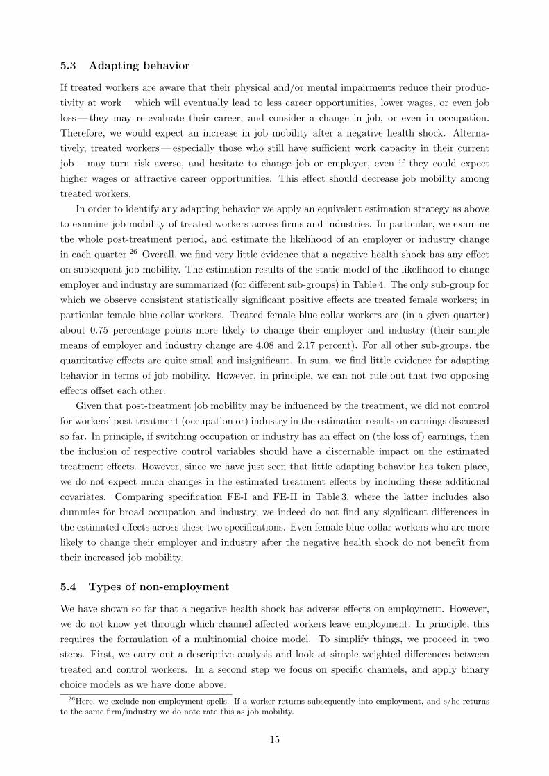
5.3 Adapting behavior

If treated workers are aware that their physical and/or mental impairments reduce their produc-

tivity at work—which will eventually lead to less career opportunities, lower wages, or even job

loss— they may re-evaluate their career, and consider a change in job, or even in occupation.

Therefore, we would expect an increase in job mobility after a negative health shock. Alterna-

tively, treated workers—especially those who still have sufficient work capacity in their current

job—may turn risk averse, and hesitate to change job or employer, even if they could expect

higher wages or attractive career opportunities. This effect should decrease job mobility among

treated workers.

In order to identify any adapting behavior we apply an equivalent estimation strategy as above

to examine job mobility of treated workers across firms and industries. In particular, we examine

the whole post-treatment period, and estimate the likelihood of an employer or industry change

in each quarter.26 Overall, we find very little evidence that a negative health shock has any effect

on subsequent job mobility. The estimation results of the static model of the likelihood to change

employer and industry are summarized (for different sub-groups) in Table 4. The only sub-group for

which we observe consistent statistically significant positive effects are treated female workers; in

particular female blue-collar workers. Treated female blue-collar workers are (in a given quarter)

about 0.75 percentage points more likely to change their employer and industry (their sample

means of employer and industry change are 4.08 and 2.17 percent). For all other sub-groups, the

quantitative effects are quite small and insignificant. In sum, we find little evidence for adapting

behavior in terms of job mobility. However, in principle, we can not rule out that two opposing

effects offset each other.

Given that post-treatment job mobility may be influenced by the treatment, we did not control

for workers’ post-treatment (occupation or) industry in the estimation results on earnings discussed

so far. In principle, if switching occupation or industry has an effect on (the loss of) earnings, then

the inclusion of respective control variables should have a discernable impact on the estimated

treatment effects. However, since we have just seen that little adapting behavior has taken place,

we do not expect much changes in the estimated treatment effects by including these additional

covariates. Comparing specification FE-I and FE-II in Table 3, where the latter includes also

dummies for broad occupation and industry, we indeed do not find any significant differences in

the estimated effects across these two specifications. Even female blue-collar workers who are more

likely to change their employer and industry after the negative health shock do not benefit from

their increased job mobility.

5.4 Types of non-employment

We have shown so far that a negative health shock has adverse effects on employment. However,

we do not know yet through which channel affected workers leave employment. In principle, this

requires the formulation of a multinomial choice model. To simplify things, we proceed in two

steps. First, we carry out a descriptive analysis and look at simple weighted differences between

treated and control workers. In a second step we focus on specific channels, and apply binary

choice models as we have done above.

26Here, we exclude non-employment spells. If a worker returns subsequently into employment, and s/he returnsto the same firm/industry we do note rate this as job mobility.

15

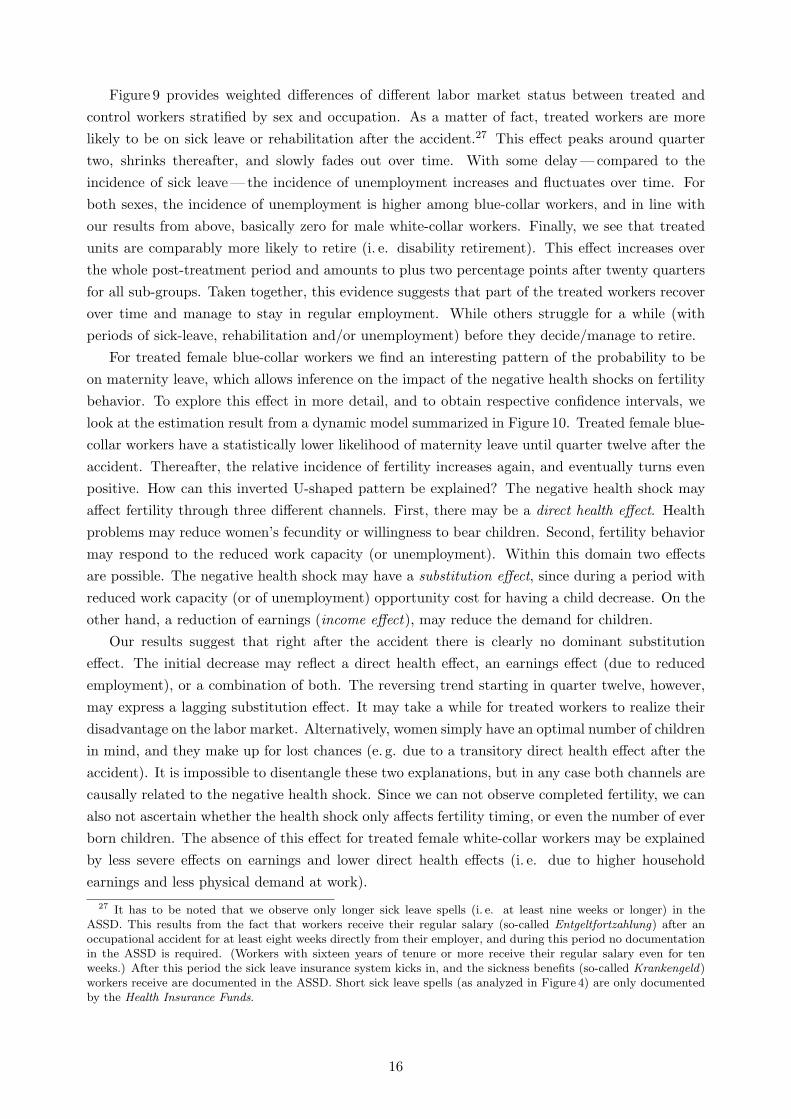
Figure 9 provides weighted differences of different labor market status between treated and

control workers stratified by sex and occupation. As a matter of fact, treated workers are more

likely to be on sick leave or rehabilitation after the accident.27 This effect peaks around quarter

two, shrinks thereafter, and slowly fades out over time. With some delay—compared to the

incidence of sick leave—the incidence of unemployment increases and fluctuates over time. For

both sexes, the incidence of unemployment is higher among blue-collar workers, and in line with

our results from above, basically zero for male white-collar workers. Finally, we see that treated

units are comparably more likely to retire (i. e. disability retirement). This effect increases over

the whole post-treatment period and amounts to plus two percentage points after twenty quarters

for all sub-groups. Taken together, this evidence suggests that part of the treated workers recover

over time and manage to stay in regular employment. While others struggle for a while (with

periods of sick-leave, rehabilitation and/or unemployment) before they decide/manage to retire.

For treated female blue-collar workers we find an interesting pattern of the probability to be

on maternity leave, which allows inference on the impact of the negative health shocks on fertility

behavior. To explore this effect in more detail, and to obtain respective confidence intervals, we

look at the estimation result from a dynamic model summarized in Figure 10. Treated female blue-

collar workers have a statistically lower likelihood of maternity leave until quarter twelve after the

accident. Thereafter, the relative incidence of fertility increases again, and eventually turns even

positive. How can this inverted U-shaped pattern be explained? The negative health shock may

affect fertility through three different channels. First, there may be a direct health effect. Health

problems may reduce women’s fecundity or willingness to bear children. Second, fertility behavior

may respond to the reduced work capacity (or unemployment). Within this domain two effects

are possible. The negative health shock may have a substitution effect, since during a period with

reduced work capacity (or of unemployment) opportunity cost for having a child decrease. On the

other hand, a reduction of earnings (income effect), may reduce the demand for children.

Our results suggest that right after the accident there is clearly no dominant substitution

effect. The initial decrease may reflect a direct health effect, an earnings effect (due to reduced

employment), or a combination of both. The reversing trend starting in quarter twelve, however,

may express a lagging substitution effect. It may take a while for treated workers to realize their

disadvantage on the labor market. Alternatively, women simply have an optimal number of children

in mind, and they make up for lost chances (e. g. due to a transitory direct health effect after the

accident). It is impossible to disentangle these two explanations, but in any case both channels are

causally related to the negative health shock. Since we can not observe completed fertility, we can

also not ascertain whether the health shock only affects fertility timing, or even the number of ever

born children. The absence of this effect for treated female white-collar workers may be explained

by less severe effects on earnings and lower direct health effects (i. e. due to higher household

earnings and less physical demand at work).

27 It has to be noted that we observe only longer sick leave spells (i. e. at least nine weeks or longer) in theASSD. This results from the fact that workers receive their regular salary (so-called Entgeltfortzahlung) after anoccupational accident for at least eight weeks directly from their employer, and during this period no documentationin the ASSD is required. (Workers with sixteen years of tenure or more receive their regular salary even for tenweeks.) After this period the sick leave insurance system kicks in, and the sickness benefits (so-called Krankengeld)workers receive are documented in the ASSD. Short sick leave spells (as analyzed in Figure 4) are only documentedby the Health Insurance Funds.

16

6 Conclusions

In this paper, we interpret accidents occurring on the way to and from work as a negative health

shock to study the causal effect of health on labor market outcomes. Data from the Austrian

mandatory social accident insurance allows us to observe the universe of these accidents which

have taken place between 2000 and 2002, and to follow these treated workers (along with exactly

matched control workers) before and after the treatment in an exhaustive administrative database.

A fixed-effects difference-in-differences approach (Heckman et al., 1997) shows a persistent

negative causal effect of this health shock on employment and earnings. Treated workers—with an

initial average sick leave spell of 46 days, predominantly due to impairments in the musculoskeletal

system—are significantly less likely to be employed throughout the whole post-treatment period.

Even after five years we still find an effect of about minus four percentage points. After initial

periods with higher incidence of sick leave (or rehabilitation), treated workers are also more likely to

be unemployed, and a growing share of them leave the labor market via disability retirement. Those

treated workers, who manage to stay or to return to employment, incur persistent earnings losses.

That means negative health shocks may result in either complete withdrawal from employment or

impede career success.

The size of the estimated effects varies along the dimensions of sex, occupation, and age.

Employment effects are strongest for sub-groups which are traditionally less attached to the labor

market, and older workers (who supposedly recover physically less well). The highest earnings

losses (about minus three percent) are observed for young workers. Somewhat surprisingly, we do

not observe much adapting behavior. Treated workers are only marginally more likely to change

job compared to control units. However, we have identified an effect of the negative health shock

on fertility behavior. Treated female blue-collar workers initially significantly reduce their fertility.

Towards the end of our period under consideration we see, however, an upward trend. Since we

can not observe completed fertility, we can not ascertain whether the health shock only affects

fertility timing, or even the number of ever born children. More generally, this result indicates

that health may have further far-reaching effects on other family outcomes, such as marriage and

divorce behavior.

Clearly, the estimated effects have to be interpreted in the light of the Austrian institutional

setting, where basically every resident has access to free health-care utilization and rehabilitation.

For two other countries—with a comparable Bismarckian (social) health insurance system—there

is evidence from a research design based on accidents available. Crichton, Stillman and Hyslop

(2011), while using all types of accidents, find for New Zealand very similar results. They also report

persistent negative employment effects and a reduction in earnings (conditional on employment);

where effects are more pronounced for sub-groups less attached to the labor market. In contrast,

Møller Danø (2005), who relies on road accidents in Denmark, finds persistent employment effects

only for males. The relative success of the Danish system in re-integrating injured female workers

might be explained by the comparable high ratio of public sector employees among females.

Unfortunately, there is no evidence available yet for countries with less pronounced social

insurance systems (such as in the U.S.). On the hand negative health shocks may have even more

detrimental effects on labor outcomes since liquidity constraints may prevent sufficient health

treatment. On the other hand, comparable less generous compensation payments in the case of

17

sickness (such as sick leave benefits or disability pensions) may increase treated workers’ incentive

to re-integrate in the labor market. In future research, it would be revealing to compare the effect

of health on earnings under different social security arrangements (see Garcıa-Gomez, 2011). This

may help to optimize the design of social insurance policies and to set the right compensation

benefits level with respect to the trade-off between sufficient protection against the risk of negative

health shocks and minimizing moral hazard.

That means the identification of the causal paths between health and earnings is not a purely

intellectual exercise, but has far-reaching implications beyond the ivory tower of academia. Causal

interpretations are also necessary to guide health and redistribution policy, or to make ethical

judgments on (health) inequality (Deaton, 2011). Having established the causal link between

health and earnings, one can argue that policies to reduce health inequality will also help to reduce

income inequality—an externality, efficient policy design has to take into account. Finally, it will

help to improve our understanding of the deeper mechanism of the accumulation of human capital

and inter-generational mobility.

References

Adda, Jerome, James Banks and Hans-Martin von Gaudecker (2009), ‘The Impact of Income

Shocks on Health: Evidence from Cohort Data’, Journal of the European Economic Association

7(6), 1361–1399.

Apouey, Benedicte and Andrew E. Clark (2010), Winning Big but Feeling No Better? The Effect

of Lottery Prizes on Physical and Mental Health, IZA Discussion Paper 4730, Institute for the

Study of Labor (IZA), Bonn (Germany).

Charles, Kerwin K. (2003), ‘The Longitudinal Structure of Earnings Losses Among Work-Limited

Disabled Workers’, Journal of Human Resources 38(3), 618–646.

Crichton, Sarah, Steven Stillman and Dean Hyslop (2011), ‘Returning to Work from Injury:

Longitudinal Evidence on Employment and Earnings’, Industrial and Labor Relations Review

64(4), 765–785.

Deaton, Angus (2011), What does the Empirical Evidence tell us about the Injustice of Health

Inequalities?, Unpublished manuscript, Center for Health and Wellbeing, Princeton University.

Deaton, Angus S. and Christina H. Paxson (1998), ‘Aging and Inequality in Income and Health’,

American Economic Review 88(2), 248–253.

Ferguson, Susan A., David F. Preusser, Adrian K. Lund, Paul L. Zador and Robert G. Ulmer

(1995), ‘Daylight Saving Time and Motor Vehicle Crashes: The Reduction in Pedestrian and

Vehicle Occupant Fatalities’, American Journal of Public Health 85(1), 92–95.

Frijters, Paul, John P. Haisken-DeNew and Michael A. Shields (2005), ‘The Causal Effect of Income

on Health: Evidence from German Reunification’, Journal of Health Economics 24(5), 997–1017.

Fuchs, Victor R (2004), ‘Reflections on the Socio-Economic Correlates of Health’, Journal of Health

Economics 23(4), 653–661.

18

Garcıa-Gomez, Pilar (2011), ‘Institutions, Health Shocks and Labour Market Outcomes Across

Europe’, Journal of Health Economics 30(1), 200–213.

Garcıa-Gomez, Pilar, Hans van Kippersluis, Owen O’Donnella and Eddy van Doorslaer (2011),

Effects of Health on Own and Spousal Employment and Income using Acute Hospital Admissions,

Discussion Paper 143/3, Tinbergen Institute.

Gardner, Jonathan and Andrew J. Oswald (2007), ‘Money and Mental Wellbeing: A Longitudinal

Study of Medium-Sized Lottery Wins’, Journal of Health Economics 26(1), 49–60.

Goldman, Noreen (2001), Social Inequalities in Health: Disentangling the Underlyng Mechanisms,

in M.Weinstein, M. A.Stoto and A. I.Hermalin, eds, ‘Population Health and Aging: Strength-

ening the Dialogue between Demography and Epidemiology’, Annals of the New York Academy

of Science, New York Academy of Sciences, New York, pp. 118–139.

Heckman, James, Hideniko Ichimura and Petra Todd (1997), ‘Matching as an Economic Evaluation

Estimator: Evidence from Evaluating a Job Training Program’, Review of Economic Studies

64(4), 605–654.

Lindahl, Mikael (2005), ‘Estimating the Effect of Income on Health and Mortality Using Lottery

Prizes as Exogenous Source of Variation in Income’, Journal of Human Resources 40(1), 144–168.

Lindeboom, Maarten, Ana Llena-Nozal and Bas van der Klaauw (2007), Health Shocks, Disability

and Work. Unpublished manuscript, Department of Economics, Free University Amsterdam.

Meer, Jonathan, Douglas L. Miller and Harvey S. Rosen (2003), ‘Exploring the Health-Wealth

Nexus’, Journal of Health Economics 22(5), 713–730.

Michaud, Pierre-Carl and Arthur van Soest (2008), ‘Health and Wealth of Elderly Couples: Causal-

ity Tests Using Dynamic Panel Data Models’, Journal of Health Economics 27(5), 1312–1325.

Møller Danø, Anne (2005), ‘Road Injuries and Long-Run Effects on Income and Employment’,

Health Economics 14(9), 955–970.

Qiu, Lin and Wilfrid A. Nixon (2008), ‘Effects of Adverse Weather on Traffic Crashes: Systematic

Review and Meta-Analysis’, Transportation Research Record: Journal of the Transportation

Research Board 2055, 139–146.

Reville, Robert T. and Robert F. Schoeni (2001), ‘Disability From Injuries at Work: The Effects

on Earnings and Employment’. RAND Corporation Publications Department, Working paper

01-08.

Riphahn, Regina T. (1999), ‘Income and Employment Effects of Health Shocks. A Test Case for

the German Welfare State’, Journal of Population Economics 12(3), 363–389.

Schwerdt, Guido, Andrea Ichino, Oliver Ruf, Rudolf Winter-Ebmer and Josef Zweimuller (2010),

‘Does the Color of the Collar Matter? Employment and Earnings after Plant Closure’, Economic

Letters 108(2), 137–140.

19

Smith, James P. (1999), ‘Healthy Bodies and Thick Wallets: The Dual Relation Between Health

and Economic Status’, Journal of Economic Perspectives 13(2), 145–166.

Strauss, John and Duncan Thomas (1998), ‘Health, Nutrition, and Economic Development’, Jour-

nal of Economic Literature 36(2), 766–817.

Thomas, Duncan, Elizabeth Frankenberg, Jed Friedman, Jean-Pierre Habicht, Mohammed Hakimi,

Nicholas Ingwersen, Jaswadi, Nathan Jones, Christopher McKelvey, Gretel Pelto, Bondan Sikoki,

Teresa Seeman, James P. Smith, Cecep Sumantri, Wayan Suriastini and Siswanto Wilopo (2006),

Causal Effect of Health on Labor Market Outcomes: Experimental Evidence, On-Line Working

Paper Series 070, California Center for Population Research.

Wagstaff, Adam (2007), ‘The Economic Consequences of Health Shocks: Evidence from Vietnam’,

Journal of Health Economics 26(1), 82–100.

Wu, Stephen (2003), ‘The Effects of Health Events on the Economic Status of Married Couples’,

Journal of Human Resources 38(1), 219–230.

Zweimuller, Josef, Rudolf Winter-Ebmer, Rafael Lalive, Andreas Kuhn, Jean-Philipe Wuellrich,

Oliver Ruf and Simon Buchi (2009), The Austrian Social Security Database (ASSD), Working

Paper 0901, The Austrian Center for Labor Economics and the Analysis of the Welfare State,

University of Linz.

20

Tables and Figures

Table 1: Average characteristics by treatment status in the quarter of the accidenta

Full sample Matched sampleb

Control Treatment Signif. Control Treatment Signif.group group of group group of

(N = 16, 813) (N = 5, 909) diff. (N = 26, 734) (N = 3, 406) diff.

Female 0.46 0.48 ** 0.51 0.51Blue-collar 0.45 0.59 *** 0.57 0.57Age 37.03 37.29 ** 37.69 37.68Academic degree 0.05 0.02 *** 0.01 0.01Non-Austrian citizenshipc 0.25 0.25 0.27 0.25 ***Tenure (in years)c 5.90 5.50 *** 6.75 6.61Experience (in years)c 15.03 14.89 15.83 15.58 *Real daily wage (in Euro) 81.48 77.54 *** 79.06 79.12Commuting distance (in km) 27.83 32.10 *** 25.93 26.13

Region of residence:West (NUTS 1) 0.37 0.35 ** 0.35 0.35East (NUTS 2) 0.42 0.40 ** 0.43 0.43South (NUTS 3) 0.21 0.25 *** 0.22 0.22Abroad or unknown 0.01 0.00 ** 0.00 0.00

Firm sizec:Overall mean 1170.94 1724.71 *** 1563.61 2114.93 ***1 to 9 0.17 0.08 *** 0.15 0.07 ***10 to 49 0.24 0.16 *** 0.20 0.14 ***50 to 99 0.10 0.11 0.10 0.10100 to 499 0.24 0.32 *** 0.26 0.32 ***500 or more 0.25 0.34 *** 0.30 0.38 ***

Industry of employer :Agriculture, fishing, mining & energy 0.02 0.02 *** 0.01 0.01Manufacturing 0.23 0.27 *** 0.29 0.29Construction 0.08 0.08 0.06 0.06Wholesale, retail & repair 0.18 0.15 *** 0.12 0.12Transport & communication 0.06 0.05 * 0.03 0.03Services 0.43 0.44 0.49 0.49

Probability of long sick leave (pre-treatment)d 0.01 0.01 0.01 0.01Sick leave resulting from accident (in days)e - 48.4 - 45.9

a This table provides the average characteristics of all individuals by treatment status measured on the first day of the quarter ofthe (placebo) accident in the full sample and in the matched sample. *, ** and *** indicate statistical significance of the differencein the average characteristics at the 10-percent level, 5-percent level, and 1-percent level, respectively. b Exact matching of treatedand control units is based on the following characteristics measured on the first day of the quarter of the (placebo) accident: sex, age(13 age groups: 25−26, 27−28, . . . , 49−50), education (no academic degree, engineer, MA/MSc, PhD), region of residence (West,East, South, abroad/missing), industry (agriculture, fishing, mining and energy; manufacturing; construction; wholesale, retail andrepair; transport and communication; services) and commuting distance (by quintile group plus additional groups for zero andmissing distance). Note, engineer (‘Ing.’) is a legally protected professional title that is granted to graduates from higher vocationalschools with technical orientation after three years of work experience. Further criteria are the employment status (employed,not employed), broad occupation (blue-collar, white-collar), and the log of the deflated daily wage rate (by decile groups plus anadditional group for non-employed individuals) in the quarter of the treatment and in each of the three preceding quarters. Furtherwe use the quarter of the (placebo) accident as a matching criterion. Note, some treated subjects may have more control subjectsthan others; to account for that weights are used. c Characteristic has not been matching criteria. d See, footnote 27 for a definitionof long (vs. short) sick leave spells. e This information is provided in the AWCB Database.

21

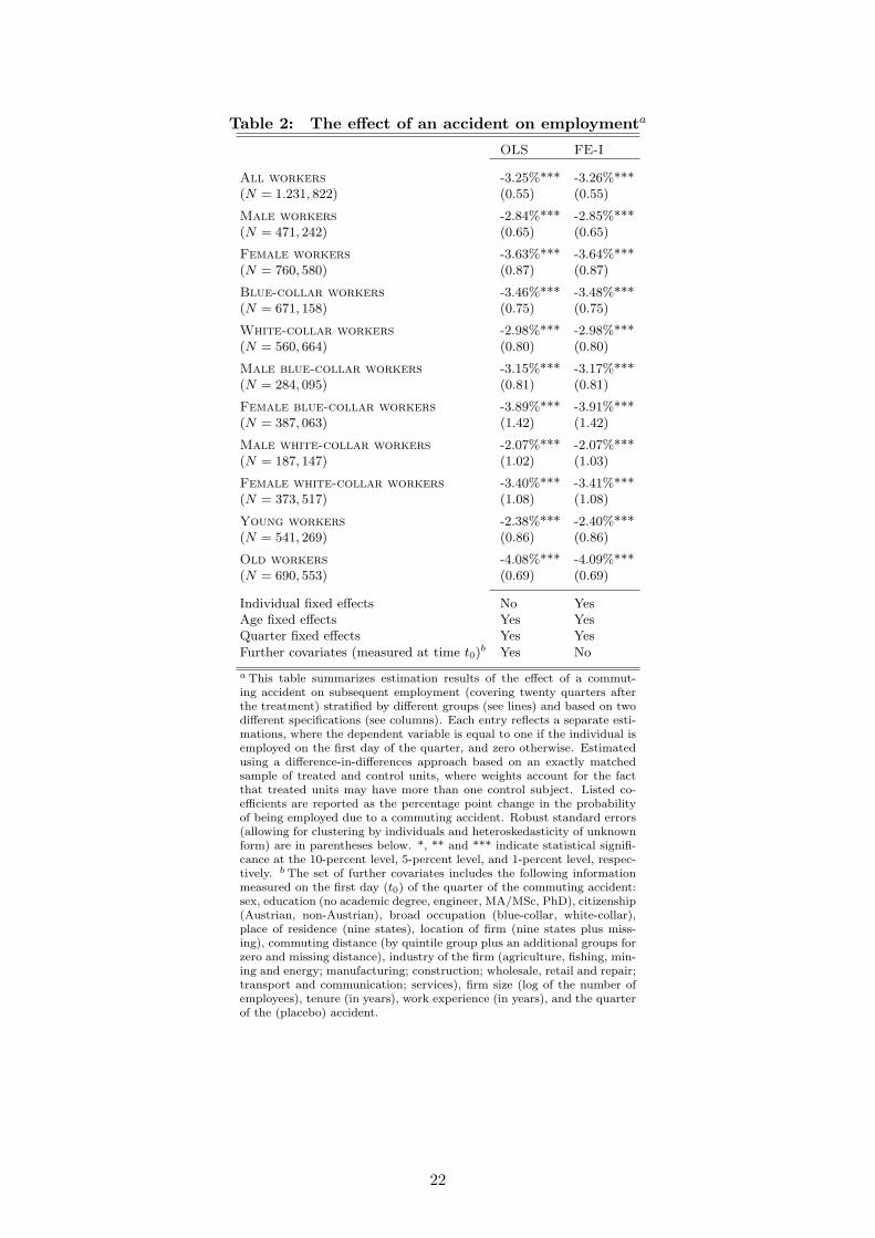
Table 2: The effect of an accident on employmenta

OLS FE-I

All workers -3.25%*** -3.26%***(N = 1.231, 822) (0.55) (0.55)

Male workers -2.84%*** -2.85%***(N = 471, 242) (0.65) (0.65)

Female workers -3.63%*** -3.64%***(N = 760, 580) (0.87) (0.87)

Blue-collar workers -3.46%*** -3.48%***(N = 671, 158) (0.75) (0.75)

White-collar workers -2.98%*** -2.98%***(N = 560, 664) (0.80) (0.80)

Male blue-collar workers -3.15%*** -3.17%***(N = 284, 095) (0.81) (0.81)

Female blue-collar workers -3.89%*** -3.91%***(N = 387, 063) (1.42) (1.42)

Male white-collar workers -2.07%*** -2.07%***(N = 187, 147) (1.02) (1.03)

Female white-collar workers -3.40%*** -3.41%***(N = 373, 517) (1.08) (1.08)

Young workers -2.38%*** -2.40%***(N = 541, 269) (0.86) (0.86)

Old workers -4.08%*** -4.09%***(N = 690, 553) (0.69) (0.69)

Individual fixed effects No YesAge fixed effects Yes YesQuarter fixed effects Yes Yes

Further covariates (measured at time t0)b Yes No

a This table summarizes estimation results of the effect of a commut-ing accident on subsequent employment (covering twenty quarters afterthe treatment) stratified by different groups (see lines) and based on twodifferent specifications (see columns). Each entry reflects a separate esti-mations, where the dependent variable is equal to one if the individual isemployed on the first day of the quarter, and zero otherwise. Estimatedusing a difference-in-differences approach based on an exactly matchedsample of treated and control units, where weights account for the factthat treated units may have more than one control subject. Listed co-efficients are reported as the percentage point change in the probabilityof being employed due to a commuting accident. Robust standard errors(allowing for clustering by individuals and heteroskedasticity of unknownform) are in parentheses below. *, ** and *** indicate statistical signifi-cance at the 10-percent level, 5-percent level, and 1-percent level, respec-tively. b The set of further covariates includes the following informationmeasured on the first day (t0) of the quarter of the commuting accident:sex, education (no academic degree, engineer, MA/MSc, PhD), citizenship(Austrian, non-Austrian), broad occupation (blue-collar, white-collar),place of residence (nine states), location of firm (nine states plus miss-ing), commuting distance (by quintile group plus an additional groups forzero and missing distance), industry of the firm (agriculture, fishing, min-ing and energy; manufacturing; construction; wholesale, retail and repair;transport and communication; services), firm size (log of the number ofemployees), tenure (in years), work experience (in years), and the quarterof the (placebo) accident.

22

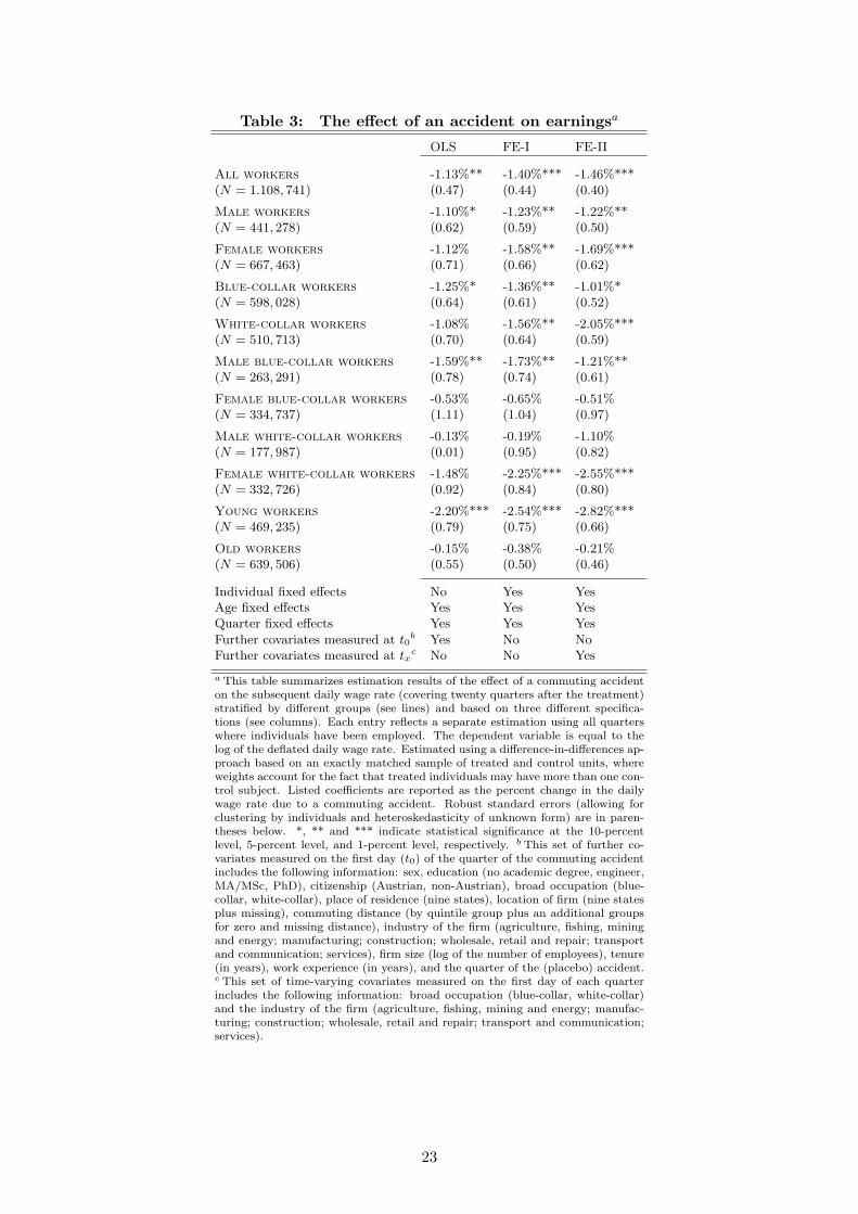
Table 3: The effect of an accident on earningsa

OLS FE-I FE-II

All workers -1.13%** -1.40%*** -1.46%***(N = 1.108, 741) (0.47) (0.44) (0.40)

Male workers -1.10%* -1.23%** -1.22%**(N = 441, 278) (0.62) (0.59) (0.50)

Female workers -1.12% -1.58%** -1.69%***(N = 667, 463) (0.71) (0.66) (0.62)

Blue-collar workers -1.25%* -1.36%** -1.01%*(N = 598, 028) (0.64) (0.61) (0.52)

White-collar workers -1.08% -1.56%** -2.05%***(N = 510, 713) (0.70) (0.64) (0.59)

Male blue-collar workers -1.59%** -1.73%** -1.21%**(N = 263, 291) (0.78) (0.74) (0.61)

Female blue-collar workers -0.53% -0.65% -0.51%(N = 334, 737) (1.11) (1.04) (0.97)

Male white-collar workers -0.13% -0.19% -1.10%(N = 177, 987) (0.01) (0.95) (0.82)

Female white-collar workers -1.48% -2.25%*** -2.55%***(N = 332, 726) (0.92) (0.84) (0.80)

Young workers -2.20%*** -2.54%*** -2.82%***(N = 469, 235) (0.79) (0.75) (0.66)

Old workers -0.15% -0.38% -0.21%(N = 639, 506) (0.55) (0.50) (0.46)

Individual fixed effects No Yes YesAge fixed effects Yes Yes YesQuarter fixed effects Yes Yes Yes

Further covariates measured at t0b Yes No No

Further covariates measured at txc No No Yes

a This table summarizes estimation results of the effect of a commuting accidenton the subsequent daily wage rate (covering twenty quarters after the treatment)stratified by different groups (see lines) and based on three different specifica-tions (see columns). Each entry reflects a separate estimation using all quarterswhere individuals have been employed. The dependent variable is equal to thelog of the deflated daily wage rate. Estimated using a difference-in-differences ap-proach based on an exactly matched sample of treated and control units, whereweights account for the fact that treated individuals may have more than one con-trol subject. Listed coefficients are reported as the percent change in the dailywage rate due to a commuting accident. Robust standard errors (allowing forclustering by individuals and heteroskedasticity of unknown form) are in paren-theses below. *, ** and *** indicate statistical significance at the 10-percentlevel, 5-percent level, and 1-percent level, respectively. b This set of further co-variates measured on the first day (t0) of the quarter of the commuting accidentincludes the following information: sex, education (no academic degree, engineer,MA/MSc, PhD), citizenship (Austrian, non-Austrian), broad occupation (blue-collar, white-collar), place of residence (nine states), location of firm (nine statesplus missing), commuting distance (by quintile group plus an additional groupsfor zero and missing distance), industry of the firm (agriculture, fishing, miningand energy; manufacturing; construction; wholesale, retail and repair; transportand communication; services), firm size (log of the number of employees), tenure(in years), work experience (in years), and the quarter of the (placebo) accident.c This set of time-varying covariates measured on the first day of each quarterincludes the following information: broad occupation (blue-collar, white-collar)and the industry of the firm (agriculture, fishing, mining and energy; manufac-turing; construction; wholesale, retail and repair; transport and communication;services).

23

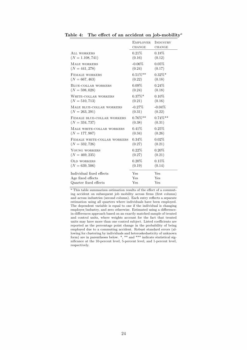
Table 4: The effect of an accident on job-mobilitya

Employer Industry

change change

All workers 0.21% 0.18%(N = 1.108, 741) (0.16) (0.12)

Male workers -0.06% 0.05%(N = 441, 278) (0.24) (0.17)

Female workers 0.51%** 0.32%*(N = 667, 463) (0.22) (0.18)

Blue-collar workers 0.09% 0.24%(N = 598, 028) (0.24) (0.18)

White-collar workers 0.37%* 0.10%(N = 510, 713) (0.21) (0.16)

Male blue-collar workers -0.27% -0.04%(N = 263, 291) (0.31) (0.22)

Female blue-collar workers 0.76%** 0.74%**(N = 334, 737) (0.38) (0.31)

Male white-collar workers 0.41% 0.25%(N = 177, 987) (0.34) (0.26)

Female white-collar workers 0.34% 0.02%(N = 332, 726) (0.27) (0.21)

Young workers 0.22% 0.20%(N = 469, 235) (0.27) (0.21)

Old workers 0.20% 0.15%(N = 639, 506) (0.19) (0.14)

Individual fixed effects Yes YesAge fixed effects Yes YesQuarter fixed effects Yes Yes

a This table summarizes estimation results of the effect of a commut-ing accident on subsequent job mobility across firms (first column)and across industries (second column). Each entry reflects a separateestimation using all quarters where individuals have been employed.The dependent variable is equal to one if the individual is changingemployer/industry, and zero otherwise. Estimated using a difference-in-differences approach based on an exactly matched sample of treatedand control units, where weights account for the fact that treatedunits may have more than one control subject. Listed coefficients arereported as the percentage point change in the probability of beingemployed due to a commuting accident. Robust standard errors (al-lowing for clustering by individuals and heteroskedasticity of unknownform) are in parentheses below. *, ** and *** indicate statistical sig-nificance at the 10-percent level, 5-percent level, and 1-percent level,respectively.

24

Figure 1: Distribution of commuting accidents by weeks on sick leave

05

10

15

20

25

30

35

Pe

rce

nt

0 1 2 3 4 5 6 7 8 9 10 11 12 13 14 15 16 17 18 19 20

Weeks

Notes: N = 11, 397, Median= 2, Mean= 4.1, S.D.= 6.8, Min= 0.14, Max= 89.

25

Figure 2: Distribution of commuting accidents by weekday and daytime (stratifiedby sex-occupation group)a

05

10

15

20

25

30

05

10

15

20

25

30

Mo Tu We Th Fr Sa Su Mo Tu We Th Fr Sa Su

Male blue-collar workers Female blue-collar workers

Male white-collar workers Female white-collar workers

Pe

rce

nt

Weekday

05

10

15

20

25

05

10

15

20

25

0 2 4 6 8 10 12 14 16 18 20 22 24 0 2 4 6 8 10 12 14 16 18 20 22 24

Male blue-collar workers Female blue-collar workers

Male white-collar workers Female white-collar workers

Pe

rce

nt

Daytime

a These graphs show the distribution of commuting accidents by weekday (upper panel) and daytime(lower panel) based on the sample of the 5, 909 treated individuals with a least two weeks of sickleave after the commuting accident.

26

Figure 3: Employment rate and earnings by treatment statusa

.5.5

5.6

.65

.7.7

5.8

.85

.9.9

51

Em

plo

ym

ent ra

te

-20 -16 -12 -8 -4 0 4 8 12 16 20

44.0

54.1

4.1

54.2

4.2

54.3

4.3

54.4

De

fla

ted

da

ily w

ag

e in

lo

gs

-20 -16 -12 -8 -4 0 4 8 12 16 20

Quarters since (potential) accident

Treatment group Control group

a These graphs show the employment rate and the average deflated daily log wage (conditional on employment) of allindividuals by treatment status. The number of treated individuals is 5, 909, and the number of control individuals is16, 813.

27

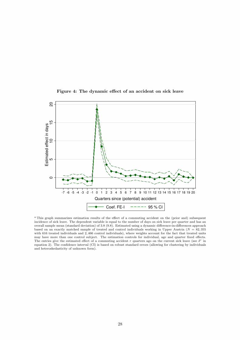
Figure 4: The dynamic effect of an accident on sick leave

05

10

15

20

Estim

ate

d e

ffect in

days

-7 -6 -5 -4 -3 -2 -1 0 1 2 3 4 5 6 7 8 9 10 11 12 13 14 15 16 17 18 19 20

Quarters since (potential) accident

Coef. FE-I 95 % CI

a This graph summarizes estimation results of the effect of a commuting accident on the (prior and) subsequentincidence of sick leave. The dependent variable is equal to the number of days on sick leave per quarter and has anoverall sample mean (standard deviation) of 3.8 (9.8). Estimated using a dynamic difference-in-differences approachbased on an exactly matched sample of treated and control individuals working in Upper Austria (N = 82, 355with 616 treated individuals and 2, 466 control individuals), where weights account for the fact that treated unitsmay have more than one control subject. The estimation controls for individual, age and quarter fixed effects.The entries give the estimated effect of a commuting accident r quarters ago on the current sick leave (see δr inequation 2). The confidence interval (CI) is based on robust standard errors (allowing for clustering by individualsand heteroskedasticity of unknown form).

28

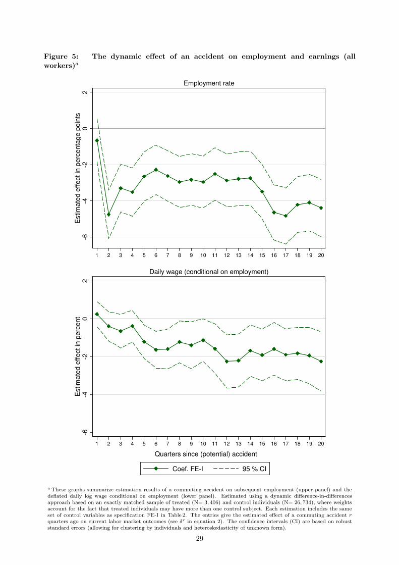
Figure 5: The dynamic effect of an accident on employment and earnings (allworkers)a

-6-4

-20

2E

stim

ate

d e

ffect in

perc

enta

ge p

oin

ts

1 2 3 4 5 6 7 8 9 10 11 12 13 14 15 16 17 18 19 20

Employment rate-6

-4-2

02

Estim

ate

d e

ffe

ct in

pe

rce

nt

1 2 3 4 5 6 7 8 9 10 11 12 13 14 15 16 17 18 19 20

Daily wage (conditional on employment)

Quarters since (potential) accident

Coef. FE-I 95 % CI

a These graphs summarize estimation results of a commuting accident on subsequent employment (upper panel) and thedeflated daily log wage conditional on employment (lower panel). Estimated using a dynamic difference-in-differencesapproach based on an exactly matched sample of treated (N= 3, 406) and control individuals (N= 26, 734), where weightsaccount for the fact that treated individuals may have more than one control subject. Each estimation includes the sameset of control variables as specification FE-I in Table 2. The entries give the estimated effect of a commuting accident r

quarters ago on current labor market outcomes (see δr in equation 2). The confidence intervals (CI) are based on robuststandard errors (allowing for clustering by individuals and heteroskedasticity of unknown form).

29

Figure 6: The dynamic effect of an accident on employment (by sex-occupation group)a

-8-6

-4-2

02

Estim

ate

d e

ffect in

perc

enta

ge p

oin

ts

1 2 3 4 5 6 7 8 9 10 11 12 13 14 15 16 17 18 19 20

Male blue-collar workers

-8-6

-4-2

02

Estim

ate

d e

ffect in

perc

enta

ge p

oin

ts

1 2 3 4 5 6 7 8 9 10 11 12 13 14 15 16 17 18 19 20

Male white-collar workers

-12

-10

-8-6

-4-2

02

Estim

ate

d e

ffect in

perc

enta

ge p

oin

ts

1 2 3 4 5 6 7 8 9 10 11 12 13 14 15 16 17 18 19 20

Female blue-collar workers

-12

-10

-8-6

-4-2

02

Estim

ate

d e

ffect in

perc

enta

ge p

oin

ts

1 2 3 4 5 6 7 8 9 10 11 12 13 14 15 16 17 18 19 20

Female white-collar workers

Quarters since (potential) accident

Coef. FE-I 95 % CI

a These graphs summarize estimation results of a commuting accident on subsequent employment for four sub-groups of workers, which are equivalent to theresults presented in the upper panel of Figure 5 for the full sample of workers. See, notes to Figure 5. Male blue-collar workers: N = 1, 187 treated and N = 5, 760control workers; female blue-collar workers: N = 756 treated and N = 8, 704 control workers; male blue-collar workers: N = 491 treated and N = 4, 094 controlworkers; female blue-collar workers: N = 972 treated and N = 8, 176 control workers.

30

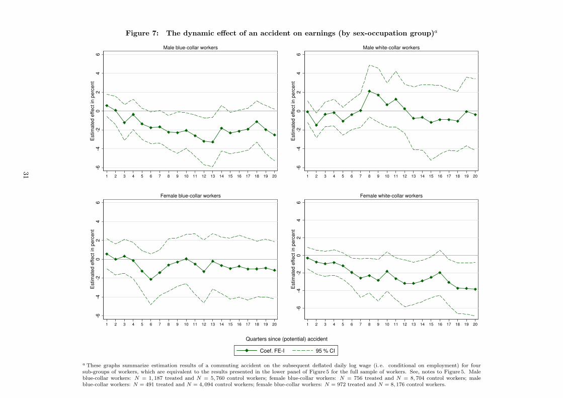
Figure 7: The dynamic effect of an accident on earnings (by sex-occupation group)a

-6-4

-20

24

6E

stim

ate

d e

ffe

ct in

pe

rce

nt

1 2 3 4 5 6 7 8 9 10 11 12 13 14 15 16 17 18 19 20

Male blue-collar workers

-6-4

-20

24

6E

stim

ate

d e

ffe

ct in

pe

rce

nt

1 2 3 4 5 6 7 8 9 10 11 12 13 14 15 16 17 18 19 20

Male white-collar workers

-6-4

-20

24

6E

stim

ate

d e

ffe

ct in

pe

rce

nt

1 2 3 4 5 6 7 8 9 10 11 12 13 14 15 16 17 18 19 20

Female blue-collar workers

-6-4

-20

24

6E

stim

ate

d e

ffe

ct in

pe

rce

nt

1 2 3 4 5 6 7 8 9 10 11 12 13 14 15 16 17 18 19 20

Female white-collar workers

Quarters since (potential) accident

Coef. FE-I 95 % CI

a These graphs summarize estimation results of a commuting accident on the subsequent deflated daily log wage (i. e. conditional on employment) for foursub-groups of workers, which are equivalent to the results presented in the lower panel of Figure 5 for the full sample of workers. See, notes to Figure 5. Maleblue-collar workers: N = 1, 187 treated and N = 5, 760 control workers; female blue-collar workers: N = 756 treated and N = 8, 704 control workers; maleblue-collar workers: N = 491 treated and N = 4, 094 control workers; female blue-collar workers: N = 972 treated and N = 8, 176 control workers.

31

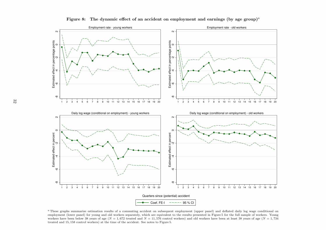
Figure 8: The dynamic effect of an accident on employment and earnings (by age group)a

-8-6

-4-2

02

Estim

ate

d e

ffect in

perc

enta

ge p

oin

ts

1 2 3 4 5 6 7 8 9 10 11 12 13 14 15 16 17 18 19 20

Employment rate - young workers

-8-6

-4-2

02

Estim

ate

d e

ffect in

perc

enta

ge p

oin

ts

1 2 3 4 5 6 7 8 9 10 11 12 13 14 15 16 17 18 19 20

Employment rate - old workers

-8-6

-4-2

02

Estim

ate

d e

ffe

ct in

pe

rce

nt

1 2 3 4 5 6 7 8 9 10 11 12 13 14 15 16 17 18 19 20

Daily log wage (conditional on employment) - young workers

-8-6

-4-2

02

Estim

ate

d e

ffe

ct in

pe

rce

nt

1 2 3 4 5 6 7 8 9 10 11 12 13 14 15 16 17 18 19 20

Daily log wage (conditional on employment) - old workers

Quarters since (potential) accident

Coef. FE-I 95 % CI

a These graphs summarize estimation results of a commuting accident on subsequent employment (upper panel) and deflated daily log wage conditional onemployment (lower panel) for young and old workers separately, which are equivalent to the results presented in Figure 5 for the full sample of workers. Youngworkers have been below 38 years of age (N = 1, 672 treated and N = 11, 576 control workers) and old workers have been at least 38 years of age (N = 1, 734treated and 15, 158 control workers) at the time of the accident. See notes to Figure 5.

32

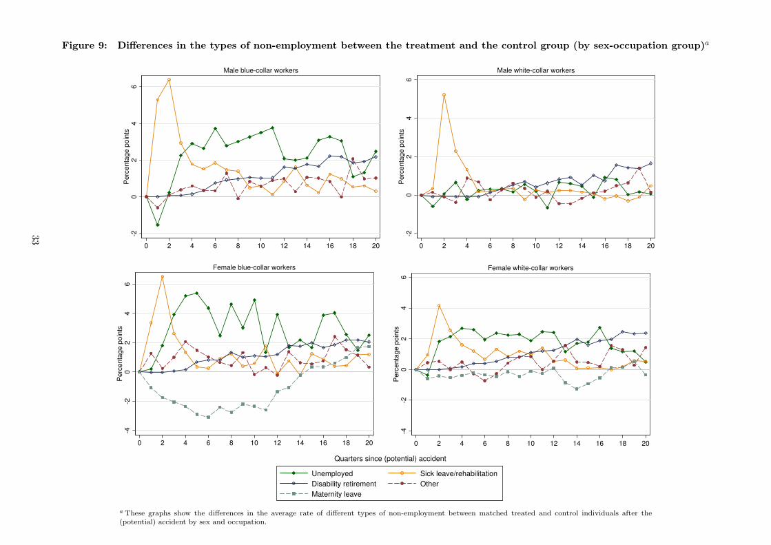
Figure 9: Differences in the types of non-employment between the treatment and the control group (by sex-occupation group)a

-20

24

6P

erc

en

tag

e p

oin

ts

0 2 4 6 8 10 12 14 16 18 20

Male blue-collar workers

-20

24

6P

erc

en

tag

e p

oin

ts

0 2 4 6 8 10 12 14 16 18 20

Male white-collar workers

-4-2

02

46

Pe

rce

nta

ge

po

ints

0 2 4 6 8 10 12 14 16 18 20

Female blue-collar workers

-4-2

02

46

Pe

rce

nta

ge

po

ints

0 2 4 6 8 10 12 14 16 18 20

Female white-collar workers

Quarters since (potential) accident

Unemployed Sick leave/rehabilitation

Disability retirement Other

Maternity leave

a These graphs show the differences in the average rate of different types of non-employment between matched treated and control individuals after the(potential) accident by sex and occupation.

33

Figure 10: The dynamic effect of an accident on the subsequent probability to be onmaternity leave (female workers by occupation)a

-4-3

-2-1

01

23

4E

stim

ate

d e

ffect in

perc

enta

ge p

oin

ts

1 2 3 4 5 6 7 8 9 10 11 12 13 14 15 16 17 18 19 20

Female blue-collar workers-4

-3-2

-10

12

34

Estim

ate

d e

ffect in

perc

enta

ge p

oin

ts

1 2 3 4 5 6 7 8 9 10 11 12 13 14 15 16 17 18 19 20

Female white-collar workers

Quarters since (potential) accident

Coef. FE-I 95 % CI

a These graphs summarize estimation results of a commuting accident on the subsequent probability to be on maternityleave. Estimated using a dynamic difference-in-differences approach based on an exactly matched sample of treated andcontrol females, where weights account for the fact that treated females may have more than one control subject. Eachestimation includes the same set of control variables as specification FE-I in Table 2 and is based on the same number ofobservations. The entries give the estimated effect of a commuting accident r quarters ago on the current probability ofbeing on maternity leave (see δr in equation 2). The confidence intervals (CI) are based on robust standard errors (allowingfor clustering by individuals and heteroskedasticity of unknown form).

34

Appendix A Additional tables and figures

A.1

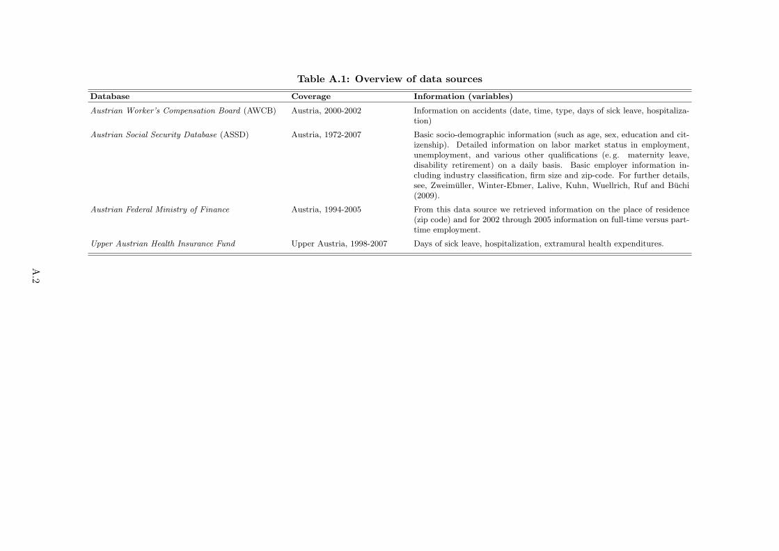
Table A.1: Overview of data sources

Database Coverage Information (variables)

Austrian Worker’s Compensation Board (AWCB) Austria, 2000-2002 Information on accidents (date, time, type, days of sick leave, hospitaliza-tion)

Austrian Social Security Database (ASSD) Austria, 1972-2007 Basic socio-demographic information (such as age, sex, education and cit-izenship). Detailed information on labor market status in employment,unemployment, and various other qualifications (e. g. maternity leave,disability retirement) on a daily basis. Basic employer information in-cluding industry classification, firm size and zip-code. For further details,see, Zweimuller, Winter-Ebmer, Lalive, Kuhn, Wuellrich, Ruf and Buchi(2009).

Austrian Federal Ministry of Finance Austria, 1994-2005 From this data source we retrieved information on the place of residence(zip code) and for 2002 through 2005 information on full-time versus part-time employment.

Upper Austrian Health Insurance Fund Upper Austria, 1998-2007 Days of sick leave, hospitalization, extramural health expenditures.

A.2

Table A.2: The effect of an accident (with hospitalization) on employmenta

OLS FE-I

All workers -5.27%*** -5.30%***(N = 354, 733) (1.06) (1.06)

Male workers -5.16%*** -5.20%***(N = 150, 735) (1.26) (1.26)

Female workers -5.37%*** -5.39%***(N = 203, 998) (1.70) (1.69)

Blue-collar workers -8.08%*** -8.11%***(N = 169, 125) (1.58) (1.58)

White-collar workers -2.47%* -2.49%*(N = 185, 608) (1.38) (1.38)

Male blue-collar workers -7.58%*** -7.61%***(N = 74, 895) (1.70) (1.70)

Female blue-collar workers -8.94%*** -8.96%***(N = 94, 230) (3.19) (3.17)

Male white-collar workers -1.13% -1.19%(N = 75, 840) (1.72) (1.73)

Female white-collar workers -3.28%* -3.30%*(N = 109, 768) (1.94) (1.94)

Young workers -3.85%** -3.88%**(N = 152, 767) (1.64) (1.64)

Old workers -6.55%*** -6.60%***(N = 201, 966) (1.35) (1.35)

Individual fixed effects No YesAge fixed effects Yes YesQuarter fixed effects Yes Yes

Further covariates (measured at time t0)b Yes No

a This table summarizes estimation results of the effect of a commut-ing accident on subsequent employment (covering twenty quarters afterthe treatment) stratified by different groups (see lines) and based on twodifferent specifications (see columns), equivalent to those presented inTable 2 in the paper, however, using only treated workers that got hos-pitalized and their matched control workers. See, notes to Table 2 in thepaper.

A.3

Table A.3: The effect of an accident (with hospitalization) on earningsa

OLS FE-I FE-II

All workers -0.32% -1.22%* -1.44%**(N = 320, 044) (0.81) (0.73) (0.70)

Male workers -1.31% -1.44% -1.80%**(N = 141, 499) (1.03) (0.97) (0.87)

Female workers 0.77% -1.03% -1.16%(N = 178, 545) (1.25) (1.10) (1.11)

Blue-collar workers -1.20% -1.95%* -2.15%**(N = 149, 430) (1.12) (1.03) (0.95)

White-collar workers 0.30% -0.65% -0.85%(N = 170, 614) (1.13) (1.03) (1.02)

Male blue-collar workers -2.09% -2.53%** -2.60%**(N = 69, 287) (1.34) (1.28) (1.08)

Female blue-collar workers 1.24% -0.59% -0.79%(N = 80, 143) (2.00) (1.70) (1.70)

Male white-collar workers -0.18% 0.30% -0.23%(N = 72, 212) (1.51) (1.45) (1.41)

Female white-collar workers 0.34% -1.27% -1.21%(N = 98, 402) (1.55) (1.41) (1.42)

Young workers -2.25*%* -2.49%** -2.67%**(N = 133, 035) (1.25) (1.16) (0.66)

Old workers 1.30% -0.14% -0.26%(N = 187, 009) (1.03) (0.93) (0.90)

Individual fixed effects No Yes YesAge fixed effects Yes Yes YesQuarter fixed effects Yes Yes Yes

Further covariates measured at t0b Yes No No

Further covariates measured at txc No No Yes

a This table summarizes estimation results of the effect of a commutingaccident on the subsequent daily wage rate (covering twenty quarters af-ter the treatment) stratified by different groups (see lines) and based onthree different specifications (see columns), equivalent to those presentedin Table 3 in the paper, however, using only treated workers that got hos-pitalized and their matched control workers. See, notes to Table 3 in thepaper.

A.4

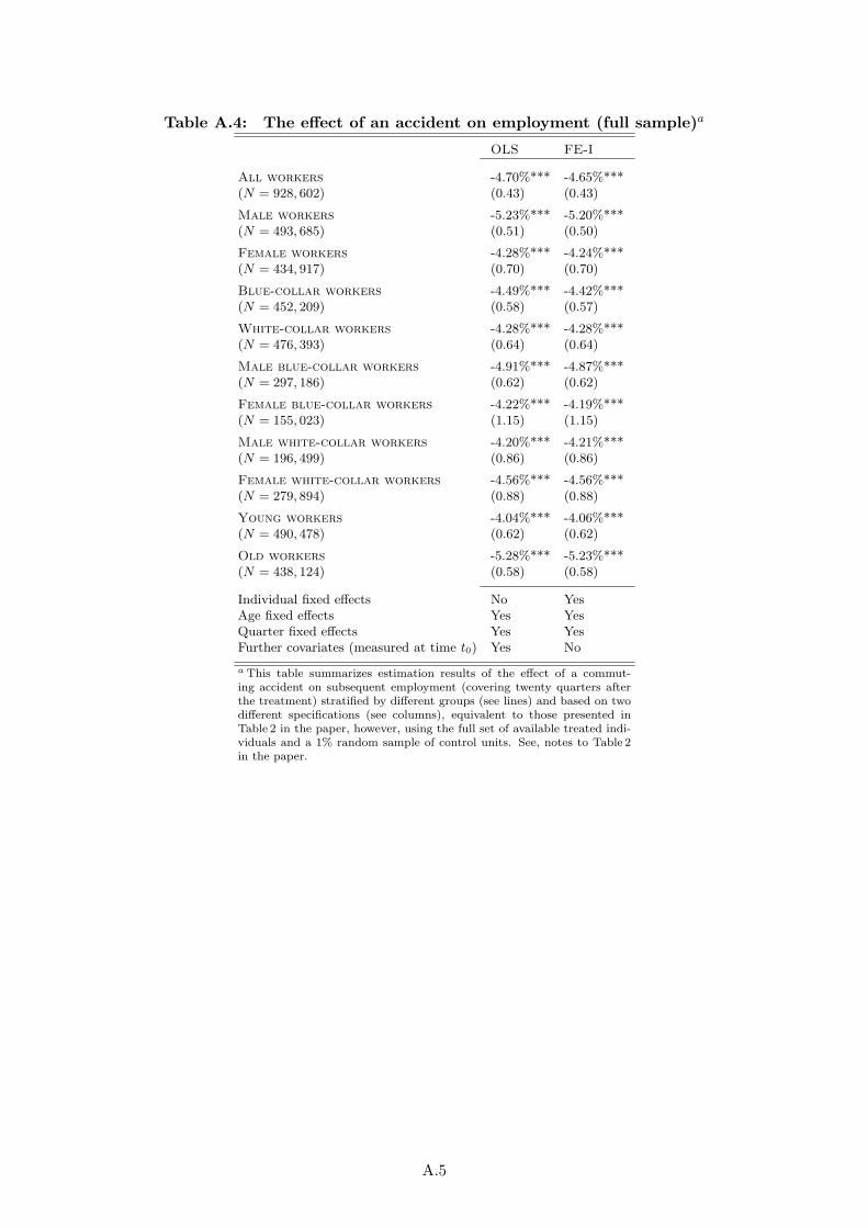
Table A.4: The effect of an accident on employment (full sample)a

OLS FE-I

All workers -4.70%*** -4.65%***(N = 928, 602) (0.43) (0.43)

Male workers -5.23%*** -5.20%***(N = 493, 685) (0.51) (0.50)

Female workers -4.28%*** -4.24%***(N = 434, 917) (0.70) (0.70)

Blue-collar workers -4.49%*** -4.42%***(N = 452, 209) (0.58) (0.57)

White-collar workers -4.28%*** -4.28%***(N = 476, 393) (0.64) (0.64)

Male blue-collar workers -4.91%*** -4.87%***(N = 297, 186) (0.62) (0.62)

Female blue-collar workers -4.22%*** -4.19%***(N = 155, 023) (1.15) (1.15)

Male white-collar workers -4.20%*** -4.21%***(N = 196, 499) (0.86) (0.86)

Female white-collar workers -4.56%*** -4.56%***(N = 279, 894) (0.88) (0.88)

Young workers -4.04%*** -4.06%***(N = 490, 478) (0.62) (0.62)

Old workers -5.28%*** -5.23%***(N = 438, 124) (0.58) (0.58)

Individual fixed effects No YesAge fixed effects Yes YesQuarter fixed effects Yes YesFurther covariates (measured at time t0) Yes No

a This table summarizes estimation results of the effect of a commut-ing accident on subsequent employment (covering twenty quarters afterthe treatment) stratified by different groups (see lines) and based on twodifferent specifications (see columns), equivalent to those presented inTable 2 in the paper, however, using the full set of available treated indi-viduals and a 1% random sample of control units. See, notes to Table 2in the paper.

A.5

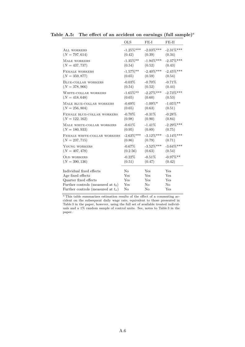
Table A.5: The effect of an accident on earnings (full sample)a

OLS FE-I FE-II

All workers -1.25%*** -2.03%*** -2.31%***(N = 797, 614) (0.42) (0.39) (0.34)

Male workers -1.35%** -1.94%*** -2.37%***(N = 437, 737) (0.54) (0.52) (0.43)

Female workers -1.57%** -2.40%*** -2.45%***(N = 359, 877) (0.65) (0.59) (0.54)

Blue-collar workers -0.03% -0.70% -0.71%(N = 378, 966) (0.54) (0.52) (0.44)

White-collar workers -1.65%** -2.27%*** -2.73%***(N = 418, 648) (0.65) (0.60) (0.53)

Male blue-collar workers -0.69% -1.09%* -1.05%**(N = 256, 804) (0.65) (0.63) (0.51)

Female blue-collar workers -0.70% -0.31% -0.28%(N = 122, 162) (0.98) (0.90) (0.84)

Male white-collar workers -0.61% -1.41% -2.29%***(N = 180, 933) (0.95) (0.89) (0.75)

Female white-collar workers -2.63%*** -3.12%*** -3.14%***(N = 237, 715) (0.86) (0.79) (0.71)

Young workers -0.67% -3.52%*** -3.64%***(N = 407, 478) (0.2.56) (0.63) (0.54)

Old workers -0.22% -0.51% -0.97%**(N = 390, 136) (0.51) (0.47) (0.42)

Individual fixed effects No Yes YesAge fixed effects Yes Yes YesQuarter fixed effects Yes Yes YesFurther controls (measured at t0) Yes No NoFurther controls (measured at tx) No No Yes

a This table summarizes estimation results of the effect of a commuting ac-cident on the subsequent daily wage rate, equivalent to those presented inTable 3 in the paper, however, using the full set of available treated individ-uals and a 1% random sample of control units. See, notes to Table 3 in thepaper.

A.6

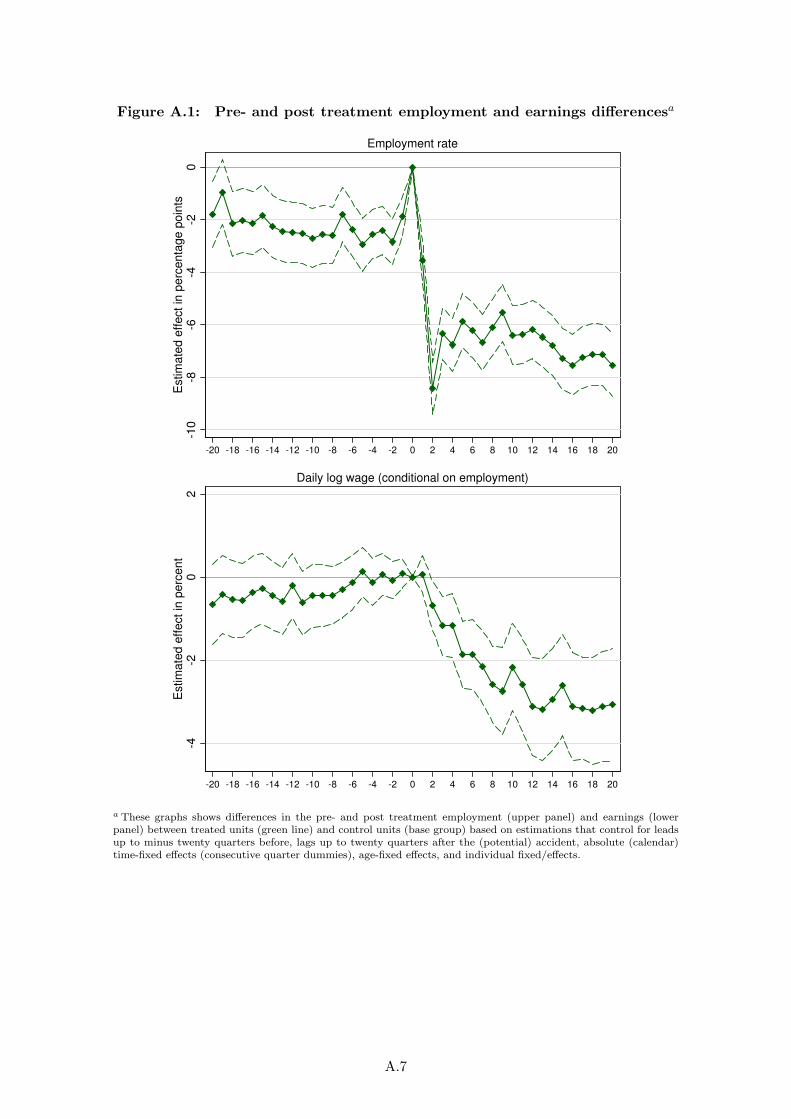
Figure A.1: Pre- and post treatment employment and earnings differencesa

-10

-8-6

-4-2

0E

stim

ate

d e

ffect in

perc

enta

ge p

oin

ts

-20 -18 -16 -14 -12 -10 -8 -6 -4 -2 0 2 4 6 8 10 12 14 16 18 20

Employment rate

-4-2

02

Estim

ate

d e

ffe

ct in

pe

rce

nt

-20 -18 -16 -14 -12 -10 -8 -6 -4 -2 0 2 4 6 8 10 12 14 16 18 20

Daily log wage (conditional on employment)

a These graphs shows differences in the pre- and post treatment employment (upper panel) and earnings (lowerpanel) between treated units (green line) and control units (base group) based on estimations that control for leadsup to minus twenty quarters before, lags up to twenty quarters after the (potential) accident, absolute (calendar)time-fixed effects (consecutive quarter dummies), age-fixed effects, and individual fixed/effects.

A.7

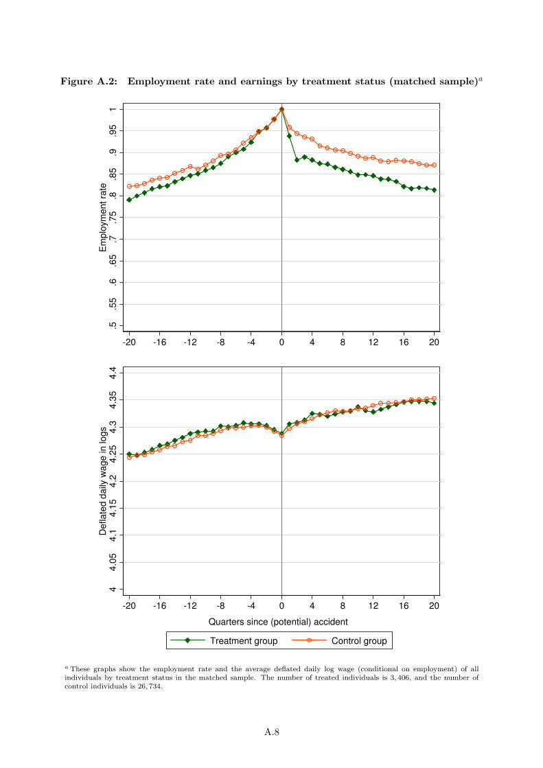
Figure A.2: Employment rate and earnings by treatment status (matched sample)a

.5.5

5.6

.65

.7.7

5.8

.85

.9.9

51

Em

plo

ym

ent ra

te

-20 -16 -12 -8 -4 0 4 8 12 16 20

44.0

54.1

4.1

54.2

4.2

54.3

4.3

54.4

De

fla

ted

da

ily w

ag

e in

lo

gs

-20 -16 -12 -8 -4 0 4 8 12 16 20

Quarters since (potential) accident

Treatment group Control group

a These graphs show the employment rate and the average deflated daily log wage (conditional on employment) of allindividuals by treatment status in the matched sample. The number of treated individuals is 3, 406, and the number ofcontrol individuals is 26, 734.

A.8

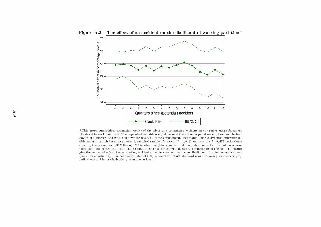
Figure A.3: The effect of an accident on the likelihood of working part-timea

-6-4

-20

24

Estim

ate

d e

ffect in

perc

enta

ge p

oin

ts

-2 -1 0 1 2 3 4 5 6 7 8 9 10 11 12

Quarters since (potential) accidentQuarters since (potential) accident

Coef. FE-I 95 % CI

a This graph summarizes estimation results of the effect of a commuting accident on the (prior and) subsequentlikelihood to work part-time. The dependent variable is equal to one if the worker is part-time employed on the firstday of the quarter, and zero if the worker has a full-time employment. Estimated using a dynamic difference-in-differences approach based on an exactly matched sample of treated (N= 1, 048) and control (N= 8, 473) individualscovering the period from 2002 through 2005, where weights account for the fact that treated individuals may havemore than one control subject. The estimation controls for individual, age and quarter fixed effects. The entriesgive the estimated effect of a commuting accident r quarters ago on the current likelihood of part-time employment(see δr in equation 2). The confidence interval (CI) is based on robust standard errors (allowing for clustering byindividuals and heteroskedasticity of unknown form).

A.9

Appendix B Health outcomes

In this section we provide further results from our supplementary analysis of the effect of a com-

muting accident on (prior and) subsequent health outcomes. Since we observe health outcomes

only for workers in Upper Austria, we have to restrict our sample to the 620 treated and 2, 482

matched control individuals working there.1 In particular, we have access to the database of the

Upper Austrian Health Insurance Fund, which covers basically all private-sector employees of Up-

per Austria. This data includes individual records from 1998 through 2007 with all covered health

services that have been provided to a worker by general practitioners (or resident medical special-

ists). That means, we can observe each single doctor visit and each drug that has been prescribed,

with the exact date of service utilization. Moreover, the database includes exact information on

sick leave spells and days of hospitalization.

In order to examine the effect of the commuting accident on health we use the following out-

comes (each measured per quarter): (i) days of sick leave, (ii) days of hospitalization, and (iii)

extramural health expenditures. For each outcome variable we estimate a dynamic model as de-

scribed by equation (2), where we in addition include leads starting at quarter minus 7. For the

incidence of hospitalization and extramural health expenditures (see FigureB.1 below) we observe

patterns, very similar to those of sick leave (as discussed in Section 4 of the paper; see Figure 4). In

the case of all three outcomes we find that the coefficients capturing the seven quarters prior to the

accident are de facto zero and do not exhibit any trend. (The base group is equal to quarter minus

eight.) In the quarter of the accident we observe a huge spike, indicating that treated workers

experience a severe negative health shock: plus 18.6 days of sick leave, plus 2 days in hospital,

and plus Euro 47.8 higher health expenditures.2 The timing clearly suggests that the commuting

accident (and not any other unobserved time-invariant factor) is the causal trigger of this negative

health shock. After the quarter of the treatment, the negative health effect decrease and dissipate

over time. The estimated effects of the accident on health outcomes are perfectly in line with the

observed dynamic effects on employment and earnings.

1Upper Austria is one of the nine states of Austria and comprises about one sixth of the Austrian population andwork force.

2Given mean values of 3.8, 0.3, and 88.2, this is equal to a 490 percent increase in sick leave, a 667 percent increasein hospital days, and 54 percent increase in health expenditures.

B.1

Figure B.1: The effect of an accident on hospitalization and extramural healthexpendituresa

-.5

0.5

11.5

22.5

3E

stim

ate

d e

ffect in

days

-7 -6 -5 -4 -3 -2 -1 0 1 2 3 4 5 6 7 8 9 10 11 12 13 14 15 16 17 18 19 20

Hospitalization

-20

-10

01

02

03

04

05

06

0E

stim

ate

d e

ffe

ct in

Eu

ros (

de

fla

ted

)

-7 -6 -5 -4 -3 -2 -1 0 1 2 3 4 5 6 7 8 9 10 11 12 13 14 15 16 17 18 19 20

Extramural health expenditures

Quarters since (potential) accident

Coef. FE-I 95 % CI

a These graphs summarizes estimation results of the effect of a commuting accident on the (prior and) subsequenthospitalization and extramural health expenditures. In the upper panel the dependent variable is equal to thenumber of days spent in hospital; this has an overall sample mean (standard deviation) of 0.3 (2.3). In the lowerpanel the dependent variable is equal to extramural health expenditures in constant Euros; this has an overallsample mean (standard deviation) of 88.2 (209.2). Estimated using a dynamic difference-in-differences approachbased on an exactly matched sample of treated and control individuals working in Upper Austria (N = 89, 822 with620 treated individuals and 2, 482 control individuals), where weights account for the fact that treated individualsmay have more than one control subject. The estimation controls for individual, age and quarter fixed effects. Theentries give the estimated effect of a commuting accident r quarters ago on the current sick leave (see δr in equation2). The confidence intervals (CI) are based on robust standard errors (allowing for clustering by individuals andheteroskedasticity of unknown form).

B.2

Appendix C Less severe accidents

In this section we present the estimated effects of less severe commuting accidents. That means, we

focus on the 5, 488 treated individuals with accidents causing less than two weeks of sick leave. After

applying an equivalent matching procedure as above we have 3, 323 matched treated and 27, 349

matched controls for our estimation analysis available (i. e. 61 percent matching rate). The average

sick leave spell in the sample of matched treated is equal to 7.6 days with a standard deviation of

3.4 days. Given the reduced accident severity we clearly expect smaller effects on subsequent labor

market outcomes compared to our main analysis of more severe accidents (i. e. at least two weeks

of sick leave) from above. TableC.1 summarizes the estimation results from the static model for

subsequent employment and earnings. These estimates can be compared with the results on more

severe accident listed in the second column in Table 2 in the paper and with the second column in

Table 3 in the paper. We see that less severe commuting accidents have smaller (or no) effects on

employment. The estimated effects on earnings (conditional on employment) are also considerably

smaller and statistically insignificant throughout. Since it seems highly unlikely that less and more

severe commuting accidents are consistently correlated with unobserved time-variant confounding

factors that have small and large effects on labor market outcomes, this analysis strongly supports

our causal interpretation from above.

C.1

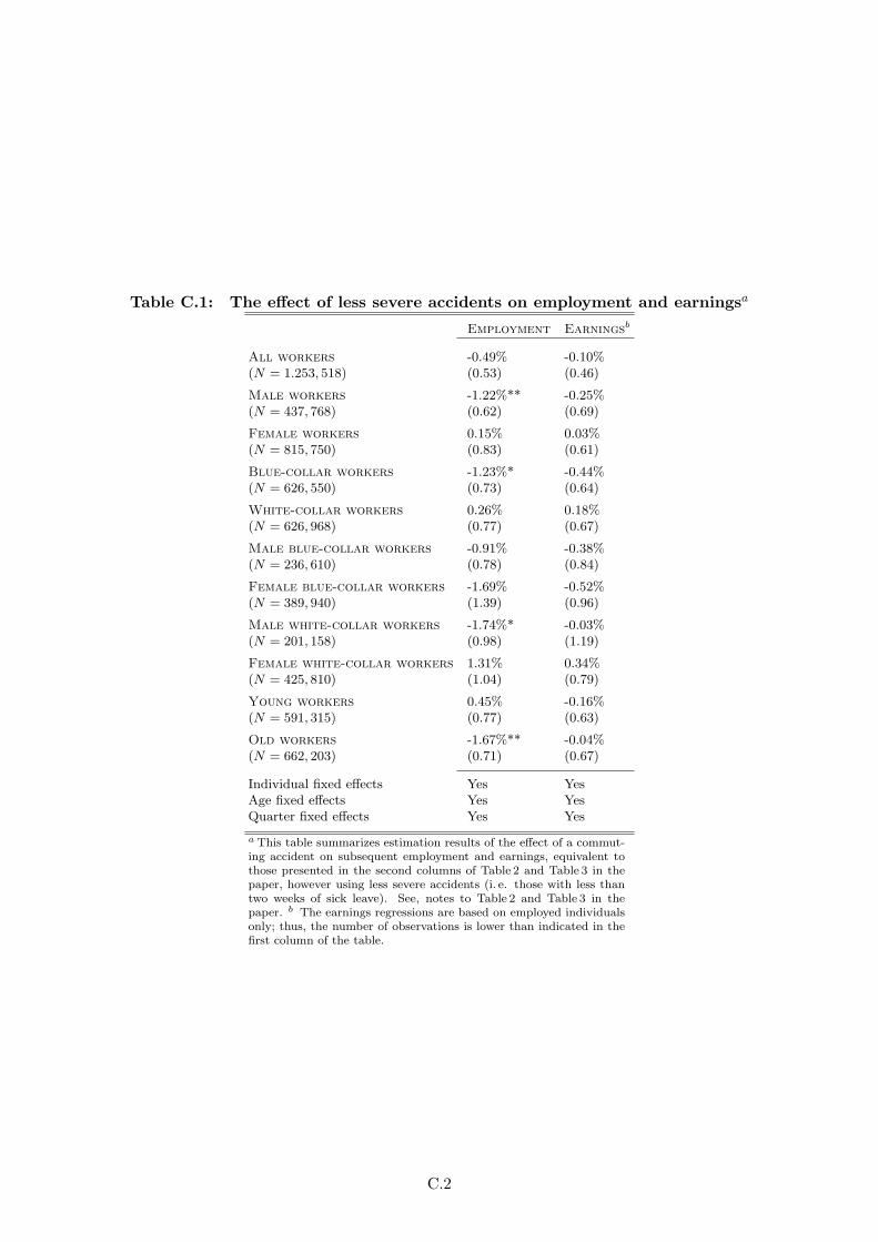
Table C.1: The effect of less severe accidents on employment and earningsa

Employment Earningsb

All workers -0.49% -0.10%(N = 1.253, 518) (0.53) (0.46)

Male workers -1.22%** -0.25%(N = 437, 768) (0.62) (0.69)

Female workers 0.15% 0.03%(N = 815, 750) (0.83) (0.61)

Blue-collar workers -1.23%* -0.44%(N = 626, 550) (0.73) (0.64)

White-collar workers 0.26% 0.18%(N = 626, 968) (0.77) (0.67)

Male blue-collar workers -0.91% -0.38%(N = 236, 610) (0.78) (0.84)

Female blue-collar workers -1.69% -0.52%(N = 389, 940) (1.39) (0.96)

Male white-collar workers -1.74%* -0.03%(N = 201, 158) (0.98) (1.19)

Female white-collar workers 1.31% 0.34%(N = 425, 810) (1.04) (0.79)

Young workers 0.45% -0.16%(N = 591, 315) (0.77) (0.63)

Old workers -1.67%** -0.04%(N = 662, 203) (0.71) (0.67)

Individual fixed effects Yes YesAge fixed effects Yes YesQuarter fixed effects Yes Yes

a This table summarizes estimation results of the effect of a commut-ing accident on subsequent employment and earnings, equivalent tothose presented in the second columns of Table 2 and Table 3 in thepaper, however using less severe accidents (i. e. those with less thantwo weeks of sick leave). See, notes to Table 2 and Table 3 in thepaper. b The earnings regressions are based on employed individualsonly; thus, the number of observations is lower than indicated in thefirst column of the table.

C.2

Appendix D Weather conditions

In this section we summarize our estimation results on the effect of weather conditions on the

likelihood of a commuting accident in the full sample. The purpose of this supplementary analysis

is twofold. First, we take weather as an example for a clear exogenous factor that affects the

likelihood of a commuting accident to support the idea that these accidents are caused by exogenous

events. Second, this analysis complements the descriptive statistics discussed in Section 2 by giving

the ceteris paribus effects of different socio-economic characteristics on the likelihood of having a

commuting accident.

To measure weather conditions on a worker’s way to and from work, we bisect the linear

distance between work and place of residence (i. e. in both cases we assume the center of the

zip-code area), and assign the closest weather station. Weather data is provided by the Central

Institute for Meteorology and Geodynamics—the national meteorological and geophysical service

of Austria. Data is collected based on 121 semi-automatic weather stations, which provide a set

of meteorological parameters (such as temperature, precipitation, relative humidity, barometric

pressure, sunshine etc.) on a hourly base. The average distance between the weather stations and

the mid-point between work and place of residence is about 8.3 kilometers (the standard deviation

is equal to 7.2 kilometers).

In the case of treated individuals, we look at the weather on the day of the commuting accident

(i. e. simple average of weather conditions between 5 am and 7 pm). For control individuals we

have randomly assigned a date from the treatment period. To define bad weather conditions we

compare different indicators measured at a weather station on a certain date (during the treatment

period) with the corresponding historical average (based on data from 1990 through 1999) from

that particular calendar day. For instance, we define a day as ‘wet’ if the precipitation on this

day is above average precipitation on this calendar day from 1990 to 1999. A linear probability

model of the likelihood of having a commuting accident including a binary variable indicating such

a wet day is summarized for female and male workers in TableD.1 below. Further covariates are

the commuting distance, month fixed effects, weekday fixed effects, region of residence fixed effects

(NUTS 3), place of work fixed effects (states), industry fixed effects, weather station fixed effects,

and a set of socio-economic variables. Based on this simple specification we find that on days

with an above average precipitation (i. e. compared to historical average at this specific location

on this specific calendar day) the likelihood of an accident increases for women (men) by 4.4 (2.0)

percentage points. Clearly, these estimates are just lower bound estimates, since we can measure

the weather conditions on a worker’s way to and from work only with error.

D.1

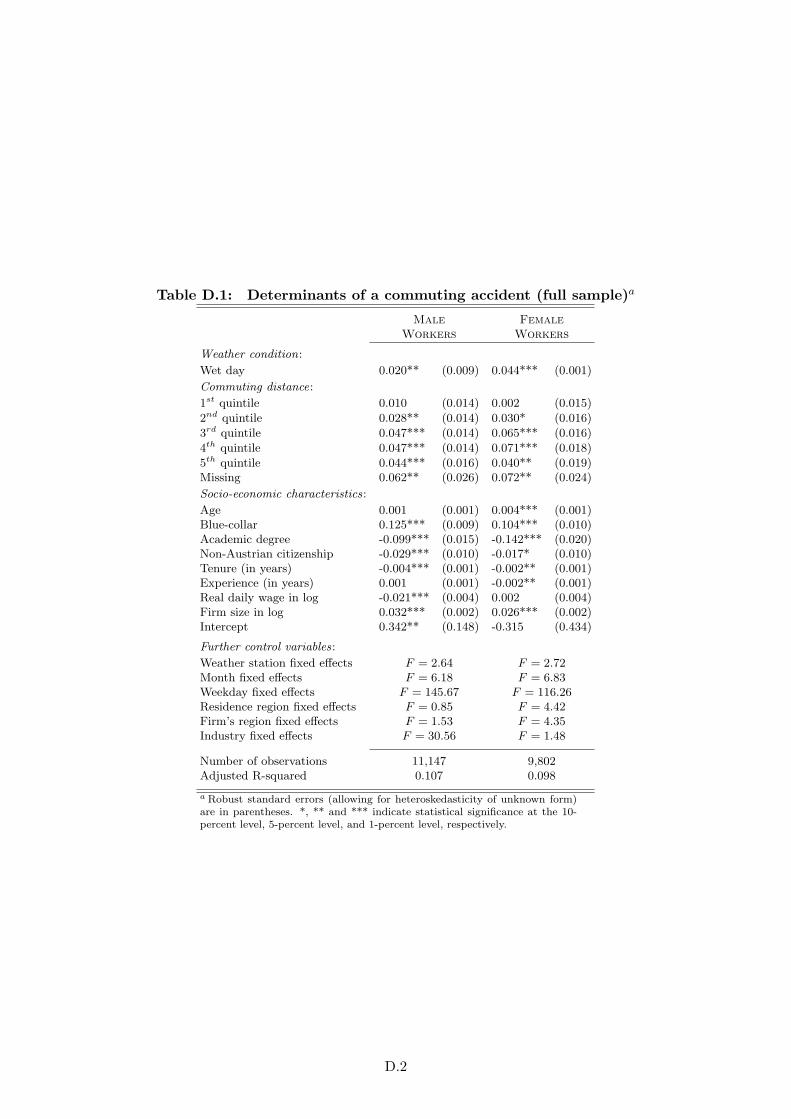
Table D.1: Determinants of a commuting accident (full sample)a

Male Female

Workers Workers

Weather condition:

Wet day 0.020** (0.009) 0.044*** (0.001)

Commuting distance:

1st quintile 0.010 (0.014) 0.002 (0.015)

2nd quintile 0.028** (0.014) 0.030* (0.016)

3rd quintile 0.047*** (0.014) 0.065*** (0.016)

4th quintile 0.047*** (0.014) 0.071*** (0.018)

5th quintile 0.044*** (0.016) 0.040** (0.019)Missing 0.062** (0.026) 0.072** (0.024)

Socio-economic characteristics:

Age 0.001 (0.001) 0.004*** (0.001)Blue-collar 0.125*** (0.009) 0.104*** (0.010)Academic degree -0.099*** (0.015) -0.142*** (0.020)Non-Austrian citizenship -0.029*** (0.010) -0.017* (0.010)Tenure (in years) -0.004*** (0.001) -0.002** (0.001)Experience (in years) 0.001 (0.001) -0.002** (0.001)Real daily wage in log -0.021*** (0.004) 0.002 (0.004)Firm size in log 0.032*** (0.002) 0.026*** (0.002)Intercept 0.342** (0.148) -0.315 (0.434)

Further control variables:

Weather station fixed effects F = 2.64 F = 2.72Month fixed effects F = 6.18 F = 6.83Weekday fixed effects F = 145.67 F = 116.26Residence region fixed effects F = 0.85 F = 4.42Firm’s region fixed effects F = 1.53 F = 4.35Industry fixed effects F = 30.56 F = 1.48

Number of observations 11,147 9,802Adjusted R-squared 0.107 0.098

a Robust standard errors (allowing for heteroskedasticity of unknown form)are in parentheses. *, ** and *** indicate statistical significance at the 10-percent level, 5-percent level, and 1-percent level, respectively.

D.2