The effect of Majorana fermions on the Andreevspectroscopy applied to topological multiband

superconductors

Ana Cristina Oliveira Silva

Thesis to obtain the Master of Science Degree in

Engineering Physics

Supervisors: Professor Pedro Domingos Santos do SacramentoProfessor Miguel António da Nova Araújo

Examination Committee

Chairperson: Professor Ana Maria Vergueiro Monteiro Cidade MourãoSupervisor: Professor Miguel António da Nova AraújoMember of the Committee: Professor Eduardo Filipe Vieira de Castro

October 2014

ii

Acknowledgments

I would like to express my sincere gratitude towards my supervisors, P.D.Sacramento and M.A.N. Araujo,

for all they have taught me and for their endless patience.

Thank you.

iii

iv

Resumo

E estudada a condutancia diferencial na interface entre um metal normal e um supercondutor topologico

com duas orbitais por sıtio da rede. As condicoes de fronteira que asseguram uma funcao de onda

contınua e injectiva foram obtidas no contexto da teoria de ”Quantum waveguide”. Na interface entre

um metal normal e um supercondutor, esta presente uma forma adicional de reflexao, a reflexao de

Andreev: um electrao incidente forma um par de Cooper na interface e e reflectida uma lacuna para a

regiao do metal normal. Um supercondutor topologico e caracterizado pela presenca de estados con-

dutores de energia nula localizados ao longo da superfıcie, “edge-states”, para os quais os operadores

de criacao coincidem com os proprios operadores de destruicao, podendo portanto ser identificados

como fermioes Majorana. O Hamiltoniano escolhido para representar o sistema permite o desacopla-

mento da matriz de Bogoliubov-De Gennes em duas matrizes 4× 4. Considerando somente um destes

sub-espacos, o sub-sistema resultante apresenta duas fases distintas - uma fase trivial e uma fase

topologica. A fase topologica caracteriza-se pela existencia de um numero de Chern nao nulo. Este

por sua vez esta interligado com o numero de “edge-states” e, portanto, com o numero de fermioes

Majorana localizados na interface. A condutancia diferencial, obtida a partir da teoria de ”Quantum

waveguide”, mostra ser consistente com o ındice topologico do sistema em contraste com a aplicacao

do modelo de Blonder-Tinkham-Klapwijck , revelando igualmente a existencia de efeitos de interferencia

destrutiva entre as bandas, nao contabilizados se estas forem consideradas independentemente.

Palavras-chave: Teoria de quantum waveguide, fermiao Majorana , supercondutor topologico,

estados ligados de Andreev, condutancia diferencial.

v

vi

Abstract

The differential conductance between a normal metal and a two-band topological superconductor is

studied. To address the wavefunction’s matching conditions at the interface, the extension of quantum

waveguide theory to the Andreev scattering problem is applied. For a normal metal-superconductor

junction, the scattering mechanism known as the Andreev reflection will occur for small energy bias.

It can be briefly defined as the process in which an incident electron will be reflected back as hole,

with the transmission of a Cooper pair into the superconductor’s side. A topological superconductor

is characterized by the existence of zero-energy conducting states at the interface which can be iden-

tified as Majorana fermions. To represent this system we considered a Hamiltonian model in which

the Bogoliubov-De Gennes matrix will split into two 4 × 4 matrices. Considering only one of these two

subspaces the subsystem can be tuned either to a trivial or topological phase by altering one of the

band structure parameters and keeping the remaining parameters fixed. The topological phase will be

characterized by a non-zero Chern number. As this quantity can be related to the number of edge-

states by the bulk-boundary correspondence, its value gives the number of localized Majorana fermions.

The calculated differential conductance within the framework of quantum waveguide theory is shown to

be consistent with the topological index, in contrast with the historically established Blonder-Tinkham-

Klapwijck model, and it also reveals the existence of destructive interference effects, which cannot be

attained if the conduction paths are treated independently.

Keywords: Quantum waveguide theory, Majorana fermion, topological superconductor, An-

dreev bound state, differential conductance

vii

viii

Contents

Acknowledgments . . . . . . . . . . . . . . . . . . . . . . . . . . . . . . . . . . . . . . . . . . . iii

Resumo . . . . . . . . . . . . . . . . . . . . . . . . . . . . . . . . . . . . . . . . . . . . . . . . . v

Abstract . . . . . . . . . . . . . . . . . . . . . . . . . . . . . . . . . . . . . . . . . . . . . . . . . vii

List of Figures . . . . . . . . . . . . . . . . . . . . . . . . . . . . . . . . . . . . . . . . . . . . . xiii

Nomenclature . . . . . . . . . . . . . . . . . . . . . . . . . . . . . . . . . . . . . . . . . . . . . . 1

1 Fundamental concepts 1

1.1 An introduction to Topological band theory . . . . . . . . . . . . . . . . . . . . . . . . . . 1

1.2 Symmetry transformations . . . . . . . . . . . . . . . . . . . . . . . . . . . . . . . . . . . . 4

1.2.1 Time-reversal symmetry and the Z2 invariant . . . . . . . . . . . . . . . . . . . . . 5

1.2.2 Particle-hole symmetry in Bogolubov-De Gennes Hamiltonians and the existence

of Majorana fermions . . . . . . . . . . . . . . . . . . . . . . . . . . . . . . . . . . 7

1.3 Kitaev’s model . . . . . . . . . . . . . . . . . . . . . . . . . . . . . . . . . . . . . . . . . . 8

1.4 Andreev spectroscopy . . . . . . . . . . . . . . . . . . . . . . . . . . . . . . . . . . . . . . 9

1.5 Overview of the BTK model . . . . . . . . . . . . . . . . . . . . . . . . . . . . . . . . . . . 14

1.6 Differential conductance and ABS in a d-wave superconductor . . . . . . . . . . . . . . . 19

1.7 Pseudo-spin . . . . . . . . . . . . . . . . . . . . . . . . . . . . . . . . . . . . . . . . . . . 22

2 Andreev spectroscopy in a multiband topological superconductor 24

2.1 The model for the Hamiltonian . . . . . . . . . . . . . . . . . . . . . . . . . . . . . . . . . 24

2.2 Quantum waveguide theory of Andreev spectroscopy . . . . . . . . . . . . . . . . . . . . . 29

2.3 Application of the waveguide theory to the N-S junction . . . . . . . . . . . . . . . . . . . 33

2.4 Differential conductance of the N-S boundary . . . . . . . . . . . . . . . . . . . . . . . . . 37

3 Conclusions and future work 45

Bibliography 49

A Derivation of the Bogolubov equations for a non-uniform superconductor 51

B Fukui-Hatsugai-Suzuki method for calculating the Chern number on a discretized Brillouin

zone. 54

ix

C The problem of finding a consistent Gauge in a two-band model 56

x

List of Figures

1.1 Representation of the Brillouin zone in 2D as a torus. . . . . . . . . . . . . . . . . . . . . . 2

1.2 Schematic representation of the Hamiltonian in eq(1.38), in a trivial (a) and non-trivial (b)

limits. . . . . . . . . . . . . . . . . . . . . . . . . . . . . . . . . . . . . . . . . . . . . . . . 9

1.3 Schematic illustration of an Andreev point contact experiment between a normal metal

(yellow) and a superconductor (blue). The Andreev reflection process is represented: an

incoming electron (red dot) enters the superconductor by forming a Cooper pair (two red

dots) and emitting a hole back (blue dot). Spin orientation is denoted by the white arrows.

Image from reference [18]. . . . . . . . . . . . . . . . . . . . . . . . . . . . . . . . . . . . 10

1.4 Schematic illustration of the tunneling transport between a normal metal and a supercon-

ductor. µN represents the chemical potential at the normal state region. In both sides the

density of states is represented: the blue color represents occupied states. Only when

µN > ∆ the current, represented by ΓN→S , will flow through the interface. Image from

reference [22]. . . . . . . . . . . . . . . . . . . . . . . . . . . . . . . . . . . . . . . . . . . 10

1.5 Normalized differential conductance as a function of the incident electron’s energy from

reference [20]. . . . . . . . . . . . . . . . . . . . . . . . . . . . . . . . . . . . . . . . . . . 11

1.6 Schematic illustration of two consecutive Andreev reflections at the interface between a

normal metal and d-wave superconductor, when the interface is oriented perpendicular to

a nodal direction. . . . . . . . . . . . . . . . . . . . . . . . . . . . . . . . . . . . . . . . . . 12

1.7 Normalized differential conductance for various barrier strengths and in two distinct cases:

a) the pairing potential is isotropic and one observes essentially the same behavior as in

fig(1.5) ; b) Normalized differential conductance corresponding to the situation described

in fig(1.6). A zero bias conductance peak appears, insensitive to the dimensionless barrier

strength Z. Image from reference [21]. . . . . . . . . . . . . . . . . . . . . . . . . . . . . . 12

1.8 Schematic representation of a normal metal- topological superconductor junction. The

red stars indicate the localized Majorana fermions. Image from reference [26]. . . . . . . 13

1.9 Quasiparticle excitations with positive group velocity in the superconductor. Image adapted

from reference [33]. . . . . . . . . . . . . . . . . . . . . . . . . . . . . . . . . . . . . . . . 17

xi

1.10 Quasiparticle excitations at both sides of the normal metal (N) - superconductor (S) in-

terface. The digits indicate the momentum of the excitations. The relevant ones indicate

as follows: 0 is the incoming electron, 2 is the transmitted excitation crossing through the

Fermi surface, 4 is the transmitted quasiparticle excitation with no Fermi surface crossing,

5 represents the normal reflection at the interface and 6 the Andreev reflection. Image

from reference [33]. . . . . . . . . . . . . . . . . . . . . . . . . . . . . . . . . . . . . . . . 17

1.11 Superconductor’s excitation spectrum. The dashed lines are the normal metal’s excitation

spectrum. Image adapted from reference [19] . . . . . . . . . . . . . . . . . . . . . . . . 18

1.12 Illustration of the scattering processes in a normal-anisotropic superconductor junction.

Image from reference [21]. . . . . . . . . . . . . . . . . . . . . . . . . . . . . . . . . . . . 20

2.1 Fermi surface and ξ+(k) band in the trivial phase. . . . . . . . . . . . . . . . . . . . . . . 28

2.2 Fermi surface and ξ+(k) band in the topological phase. . . . . . . . . . . . . . . . . . . . 28

2.3 Energy spectrum of the Hamiltonian model eq(2.7) for an infinite ribbon in the yy (or xx)

direction. The Majorana fermion can be seen for the longitudinal momentum π. This figure

was obtained by M.A.N. Araujo. . . . . . . . . . . . . . . . . . . . . . . . . . . . . . . . . 28

2.4 Node occurring at the interface between a normal metal and a two-band superconductor.

Image from reference [28]. . . . . . . . . . . . . . . . . . . . . . . . . . . . . . . . . . . . 29

2.5 Tight-binding showing the splitting of the incoming electron into two channels of the su-

perconductor, similar to a waveguide. Image from reference [28]. . . . . . . . . . . . . . 30

2.6 Tight-binding showing the splitting of the incoming electron into two pseudo-spin channels

of the superconductor, similar to a waveguide. . . . . . . . . . . . . . . . . . . . . . . . . . 33

2.7 Conductance gs and gn as function of the incident electron energy for t2 = +0.08 in a

microconstriction, Z=0, for a fixed transverse momentum py= 0. Calculation performed

with waveguide theory. . . . . . . . . . . . . . . . . . . . . . . . . . . . . . . . . . . . . . 37

2.8 Conductance gs and gn as function of the incident electron energy for t2 = +0.08 and Z=1,

for a fixed transverse momentum py=0. Calculation performed with waveguide theory. . . 38

2.9 Conductance gs and gn as function of the incident electron energy for t2 = +0.08 and Z=2,

for a fixed transverse momentum py= 0. Calculation performed with waveguide theory. . 38

2.10 Conductance gs as function of the incident electron energy for t2 = +0.08 in a microcon-

striction, Z=0, computed with BTK generalized model, for a fixed transverse momentum

py=0. . . . . . . . . . . . . . . . . . . . . . . . . . . . . . . . . . . . . . . . . . . . . . . . 39

2.11 Conductance gs and gn as function of the incident electron energy for t2 = +0.08 and Z=0,

for a fixed transverse momentum py=π. Calculation performed with waveguide theory. . . 39

2.12 Conductance gs and gn as function of the incident electron energy for t2 = +0.08 and Z=1,

for a fixed transverse momentum py=π. Calculation performed with waveguide theory. . . 40

2.13 Conductance gs and gn as function of the incident electron energy for t2 = +0.08 and Z=2,

for a fixed transverse momentum py=π. Calculation performed with waveguide theory. . . 40

xii

2.14 Conductance gs and gn as function of the incident electron energy for t2 = −0.08 and Z=0

and a fixed transverse momentum py=0. Calculation performed with waveguide theory. . 41

2.15 Conductance gs and gn as function of the incident electron energy for t2 = −0.08 and Z=1

and a fixed transverse momentum py=0. Calculation performed with waveguide theory. . 41

2.16 Conductance gs and gn as function of the incident electron energy for t2 = −0.08 and Z=2

and a fixed transverse momentum py=0. Calculation performed with waveguide theory. . 42

2.17 Conductance gs as function of the incident electron energy for t2 = −0.08 with various

strength barriers and a fixed transverse momentum py=π. Calculation performed using

the generalized BTK model. . . . . . . . . . . . . . . . . . . . . . . . . . . . . . . . . . . 42

2.18 Conductance gs as function of the incident electron energy for t2 = −0.08 with various

strength barriers and a fixed transverse momentum py=π. Calculation performed using

waveguide theory. . . . . . . . . . . . . . . . . . . . . . . . . . . . . . . . . . . . . . . . . 43

xiii

xiv

Chapter 1

Fundamental concepts

1.1 An introduction to Topological band theory

The building blocks of matter can interact in various forms, which subjected to certain external condi-

tions, can lead to different states of matter. In the theory of phase transitions, one usually defines a local

order parameter which acquires a distinct expectation value as the different phases are established. By

comparison with this framework, topological states of matter emerge as a new paradigm [1]: not only is

it impossible to define a local order parameter, but also the different topological states are differentiated

upon the inability to adiabatically deform the energy bands into one another, without closing the bulk

gap. Thus, a material in a topological phase, in contact with another in a trivial phase, has to undergo

a phase transition at the interface, accomplished by the vanishing of the bulk gap. At the points where

the bulk gap collapses, gapless conducting states arise. These states are, therefore, able to conduct

current along the interface and are known as edge-states [2, 3]. This scenario can occur, for example,

at the interface between a topological insulator and the vacuum. In this case, one can see more easily

that the appearance of such edge-states is highly interconnected to the non-trivial topology of the bulk,

a phenomena known as bulk-edge correspondence [2].

The gapless modes exhibit more robustness in face of local disorder, which is another peculiarity of the

topological phase, and are related with the existence of a non-zero topological invariant [4].

In this thesis, the dominant focus falls to one topological invariant, the Chern number (present in systems

without time-reversal symmetry), although some remarks will be given to a second invariant, the Z2 (for

time-invariant systems).

The mathematical construction of the Chern number is rooted in the Berry phase (γn) : as the Hamilto-

nian of the system is adiabatically transformed by slowly varying its parameters, the eigenstates gain a

phase, γ, which contains a new term, besides the usual dinamical phase [5] ,

γn = i

∮〈ψn(R)| ∂

∂R|ψn(R)〉 · δR . (1.1)

The function integrated in the equation above is called the Berry connection or Berry vector potential.

From this quantity we define the Berry curvature:

1

Ωn = ∇×An (1.2)

Integrating the Berry curvature over all the Brillouin zone defines the topological invariant Chern

number, an integer which is non-zero for the topological phases.

Cn =1

2π

∫TBZ

Ωn dS . (1.3)

It is important to note that this integral is directly related to the Berry phase: the integrals in eq(1.3)

and in eq(1.1) are equivalent as a result of the application of Stokes’ theorem.Therefore one can also

define the Chern number as the accumulated Berry phase around the Brillouin zone divided by 2π, which

will be invariant under a smooth gauge transformation of the eigenstates [1]. For a two-band model, a

geometric interpretation of the Chern number is also possible. In these systems, the Hamiltonian can

be written as H = h(k).σ and it can be showed that eq(1.3) counts the number of times the unit vector

h/|h| covers the entire unit sphere as a function of the momentum k [2].

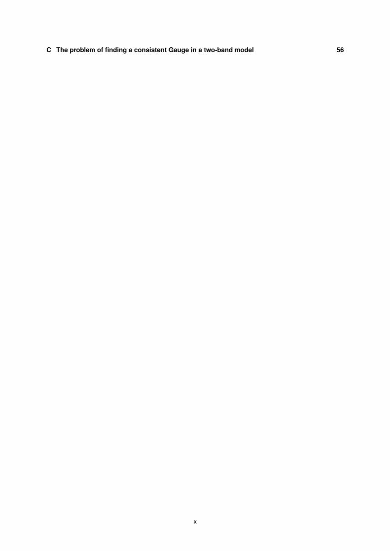
To determine the Chern number, it is necessary to solve eq(1.3). One strategy is to apply Stokes’ the-

orem. However, as the Brillouin zone is a torus (fig. 1.1) it has no boundary, so if the Berry curvature

is a well behaved function one would always obtain a zero Chern number, which is precisely what hap-

pens for non-topological phases [6]. Nevertheless, the procedure breaks down if the Berry connection

presents singularities. The origin of such problematic points lies on the impossibility of picking a global

gauge that guarantees a smooth and single-valued wavefunction [6, 3]. Instead, it is necessary to define

distinct gauges in different regions of the Brillouin zone and separately apply the Stokes’ theorem to the

different patches.

Figure 1.1: Brillouin zone in 2D. Image adapted from reference [6].

In order to clarify how this can lead to an integer number, it is useful to present the example given by

the authors B. Andrei Bernevig and Taylor L.Hughes [3]: one first considers the existence of two regions

in the Brillouin zone, R and TBZ −R. Inside each patch, it is possible to choose a local gauge such

that the wavefunction is well-behaved and vanishes when the region boundaries are crossed. Identifying

eif(k)ψ1 with the wavefunctin at TBZ−R and eig(k)ψ2 with the region R , where eif(k) and eig(k) are the

respective gauge transformations, allows to state the boundary condition as the following:

2

eif(k)ψ1 = eig(k)ψ2 (1.4)

⇔ ψ2 = e−iθ(k)ψ1, with θ(k) = g(k)− f(k) (1.5)

Accordingly, the two Berry connections are related:

A2(k) = A1(k) +∇θ(k) (1.6)

The next step is to explicitly evaluate the integral for the Chern number:

Cn =1

2π

(∫R∇×A1(k) +

∫TBZ−R

∇×A2(k))

(1.7)

Remembering that the torus has no boundary, the application of Stokes’ theorem to the last equa-

tion enables the line integral of the two connections to be calculated over the same boundary ∂R with

opposite orientations: ∂(TBZ −R) = −∂R . Then eq( 1.7 ) can then be written as:

Cn =1

2π

∫∂R

dk∇θ(k) (1.8)

Thus, the promised result has been achieved. If ∂R is a close loop, the wavefunction has to be the

same in the starting and end points which forces the previous integration to be proportional to 2π . This

is the same reasoning as to why the winding number in a vortex is quantized.

The definition of the Chern number, eq.(1.3), can yet be presented differently: one starts from explicitly

computing the Berry curvature for a given occupied band n,

Ωnkx,ky = ∇×An =∂Any∂kx

− ∂Anx∂ky

(1.9)

which by virtue of eq(1.1) becomes:

Ωnkx,ky = i[〈∂ψn∂kx|∂ψn∂ky〉 − 〈∂ψn

∂ky|∂ψn∂kx〉] (1.10)

Taking the inner product of the state 〈ψ′n| in both sides of the eigenvalue equation, H|ψ〉 = E|ψ〉 , and

differentiating the resulting equation, produces an equality similar to the Hellmann-Feynman theorem:

〈ψn′ |∂ψn∂kx〉 =

1

En − En′〈ψn′ |

∂H

∂kx|ψn〉 (1.11)

After which is possible to rewrite the state |∂ψn

∂kx〉 as a linear expansion in the eigenstates |ψn′〉 , with

coefficients for n 6= n′ given by the last equation. Hence, using this linear expansion representation of

the states |∂ψn

∂kx〉, the Berry curvature gains the new form:

Ωnkx,ky = i∑n 6=n

〈ψn| ∂H∂kx |ψn′〉〈ψn′ |∂H∂ky|ψn〉 − 〈ψn| ∂H∂ky |ψn′〉〈ψn′ |

∂H∂kx|ψn〉

(En − En′)2(1.12)

This alternative expression can be shown to be related to the Kubo formula for the Hall conductance

3

[7]:

σH =e2

h

1

2π

∫Ωnkx,kydkxdky, (1.13)

where one can recognize the integral above as the Chern number defined in eq.(1.3), thus allowing to

relate the Chern number with an observable quantity, the Hall conductance. Additionally, eq(1.9) reveals

that the sum of the Chern number of all bands must be zero, owing to the anticomutative property of the

cross product. For example, in a two-band system, taking |−〉 to be the eigenstate of the lower energy

band and |+〉 the eigenstate of the upper band, the Berry potential in each band is given by:

Ω− = i〈−|∇H(k)|+〉 × 〈+|∇H(k)|−〉

(E− − E+)2(1.14)

Ω+ = i〈+|∇H(k)|−〉 × 〈−|∇H(k)|+〉

(E+ − E−)2(1.15)

⇒ C+ = −C− , (1.16)

explicitly illustrating how the sum in all bands of the Chern number will be zero.

The Chern number can also be calculated through the bulk-boundary correspondence [2], which math-

ematically is stated in the following way: if there are NR edge states with positive group velocity and NL

with negative, the change in the change in the Chern number across the interface will be quantified by

∆C = NR −NL . (1.17)

Then if the interface demarks the separation between a trivial and a topological system, the Chern

number can be determined directly by the above equation.

1.2 Symmetry transformations

Provided that two physical systems share the same topological invariant, they are topologically equiva-

lent, which suggests that there must be some underlying symmetries enabling the division of systems

into topological classes [8].

Two important symmetries are time-reversal symmetry (TRS) and particle-hole symmetry (PHS), both

implemented by antiunitary operators on the Hilbert space. Any antiunitary operator will be defined as

the general operator A satisfying:

〈Aφ|Aψ〉 = 〈φ∗|ψ∗〉 (1.18)

Such operators will be in general represented by the complex conjugation operator (K) and an unitary

operator (U ) in the form KU , which can either be squared +1 or −1 [8, 3].

4

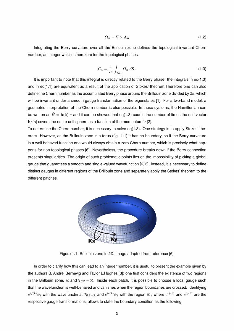
1.2.1 Time-reversal symmetry and the Z2 invariant

The single-particle Hamiltonian possesses time-reversal symmetry if it verifies [3]:

H = T HT −1 ,with: T 2 = ±1 , (1.19)

where T is the time-reversal operator. The ± sign regards two distinct cases: the + sign corresponds

to the TRS operator for spinless (or integer spin) particles, while the − sign is applicable for half-integer

spinful particles. In the spinless case, the TRS operator is simply given by the complex conjugation

operator, T = K, whereas for half-integer spin particles T = iσyK.

If the Hamiltonian of the system is said to possess TRS, the single-particle Hamiltonian in momentum

space will have to verify the conditions [8]:

H(k) = H∗(−k) Spinless particles , (1.20)

H(k) = iσyH∗(−k)(−iσy) Spinful particles . (1.21)

In the case of the superconductor’s Hamiltonian, written in the general form:

H =1

2

∑k

a†k. HBdG .ak , HBdG =

Ξ ∆

∆† −Ξ∗

, (1.22)

where ak = (ck↑ ck↓ c†−k↑ c†−k↓)T . The condition for TRS is similar to eq(1.21):

HBdG(k) = iσyH∗BdG(−k)(−iσy) . (1.23)

For spinful particles, the fact that the TRS operator squares to −1 implies that such systems obey

the Kramers’ theorem: for an odd number of particles with half-integer spin, there are at least two

degenerate eigenstates, Ψ and T Ψ [9, 3]. This result is established by proving that Ψ and T Ψ are

orthogonal eigenstates. To prove it, one first must notice that:

〈T ψ|T 2ψ〉 = 〈ψ|T ψ〉∗ , because T is anti-unitary . (1.24)

Nevertheless, for spinful particles it is also true that:

〈T ψ|T 2ψ〉 = −〈T ψ|ψ〉 = −〈ψ|T ψ〉∗ , (1.25)

and thus

〈ψ|T ψ〉∗ = −〈ψ|T ψ〉∗ ⇒ 〈ψ|T ψ〉 = 0 . (1.26)

A relevant consequence of this theorem applies to the elements of the scattering matrix 〈T Ψ|H|Ψ〉,

particularly if the scattering process concerns an odd number of excitations, then the probability of

5

scattering between the two states is zero. This can be seen by noticing that:

〈ψ|H|T ψ〉 = 〈T ψ|T HT ψ〉∗ = 〈T ψ|T HT −1T 2ψ〉∗ = 〈T ψ|HT 2ψ〉∗ = −〈T ψ|H|ψ〉∗ , (1.27)

where it has been used the time-reversal invariance of the Hamiltonian of the system (H = T HT −1).

However, because H is Hermitian, then:

〈T ψ|H|ψ〉∗ = 〈ψ|H|T ψ〉 , (1.28)

which when substituting in eq( 1.27 ), leads to:

〈ψ|H|T ψ〉 = −〈ψ|H|T ψ〉 ⇒ 〈ψ|H|T ψ〉 = 0 . (1.29)

One way of viewing the underlying implications of this result is by imagining a 2D-geometry where a

fermion moves in the x-direction. It will never be backscattered, unless TRS has been broken.

Under TRS the Berry curvature changes sign. Therefore a TRS system has C = −C = 0 [3].

In time-reversal invariant systems, a non-trivial phase will be characterized by a different topological

invariant, the Z2, which can take upon two values: ν = 0 (trivial phase) and ν = 1 (topological phase)

[2]. This topological invariant was first introduced by Kane and Mele [10] when studying the effect of

spin-orbit interaction in the Hamiltonian of a single plane of graphene. To exemplify how a topological

phase can emerge in the presence of TRS, it is sufficient to address the simplest form of the spin-orbit

term considered by these authors, in which the Sz spin component is conserved [11]. In this case, the

Hamiltonian will decouple into two independent contributions: the Hamiltonian for spin-up electrons and

the correspondent term for spin-down electrons [11]. The system altogether respects TRS, but each

spin contribution taken separately does not and hence spin-up and spin-down carry opposite Chern

numbers [11]. As a consequence, at the boundaries of the system counter-propagating edge-modes

will both appear at time-reversal invariant points, but because TRS is present, spin-up and spin-down

edge-states will not mix ( single-particle backscattering is prohibited) [3]. At other momentum points,

the spin-orbit interaction will lift the degeneracy imposed by Kramers’ theorem. The connection between

states at different time invariant points, for example k = 0 and k = π, can occur in two distinct forms,

depending on the topological properties of the bulk system. If the energy dispersion relation of each

pair crosses the Fermi energy an even number of times, there will be an even number of Kramers’ pairs

and a gap will open due to backscattering. The system will be topologically equivalent to a trivial phase.

However, if the energy dispersion relation of each pair intersects the Fermi energy an odd number of

times, backscattering cannot occur: they are protected from opening a gap by TRS and the edge-states

will propagate freely even under small perturbations, leading to the propagation of ”spin-filtered” current

[10, 3, 2]. In this case, the system is in a non-trivial phase which by analogy to the quantum hall effect

is called the quantum spin hall phase [11]. The value of the Z2 invariant can therefore be calculated by

the bulk-boundary correspondence, relating the number of Kramers’ pairs edge-states ( NK ) with the

6

change of the topological invariant at the boundary of the system (∆ν) [2]:

NK = ∆ν mod 2 (1.30)

It should be noted that the eq(1.30) is not the only way of calculating the Z2 invariant [10, 2, 3]. Other

methods include, for example, interpreting the Z2 as the obstruction to Stokes’ theorem in half of the

Brillouin zone [3].

1.2.2 Particle-hole symmetry in Bogolubov-De Gennes Hamiltonians and the

existence of Majorana fermions

The Bogolubov-De Gennes Hamiltonian (HBdG) written as in eq(1.22) has PHS, defined as [8]:

HBdG(k) = −τxH∗BdG(−k)τx ,where the Pauli matrix τx operates in particle-hole space . (1.31)

This is an intrinsic symmetry of the HBdG matrix in eq(1.22) due to the Hermiticity of Ξ and because

∆(k) = −∆T (k), by imposition of the Fermi statistics [12, 8], with the pairing potential ∆ either a singlet

or a triplet pairing [12]:

Singlet pairing: ∆(k) = ψ(k)iσy =

0 ψ(k)

−ψ(k) 0

, ψ(k) even function of k (1.32)

Triplet pairing: ∆(k) = i(d(k).σ)σy =

−dx(k) + idy(k) dz(k)

dz(k) dx(k) + idy(k)

, d(k) odd function of k .

(1.33)

The Hamiltonian in eq( 1.22 ) can be diagonalized by performing a Bogolubov transformation, allow-

ing to express the Hamiltonian in terms of the non-interacting quasiparticle operators [13]. In real space

the quasiparticle destruction operator will be:

γ =

∫dr u∗↑(r)ψ↑ + u∗↓(r)ψ↓ + v∗↑(r)ψ†↑ + v∗↓(r)ψ†↓ . (1.34)

The eigenstates of the HBdG are given by: φ(r) = (u↑(r) u↓(r) v↑(r) v↓(r))T . Eq( 1.31 ) implies

that if the eigenstate φ has energy E, the eigenstate τxφ∗ will have −E energy. Thus, if E = 0 and this

is a non-degenerate state, PHS will lead to:

φ(r) = τxφ∗(r)⇔ γ = γ† ⇒ Majorana fermion . (1.35)

In analogy with particle physics, this equality can be viewed as the equivalence between particle and

anti-particle, which is exactly the definition of a Majorana particle, or in this case, a Majorana fermion.

Superconductors are, therefore, ideal candidates for creating Majorana fermions from the quasiparticle

7

excitations [14, 15, 16].

1.3 Kitaev’s model

Conversely, it is possible to describe an usual fermion as superposition of Majorana modes [14, 15, 3].

This can be clarified by constructing an algebraic representation where the usual fermionic operators

are written in terms of Majorana operators (eq(1.35)), which satisfy [14, 15, 16]:

γi, γj = 2δij . (1.36)

The fermionic operators can then be presented as [17, 3, 14]:

cj = 12 (γ2j−1 + iγ2j)

c†j = 12 (γ2j−1 − iγ2j)

(1.37)

explicitly showing how a conventional fermion can be thought as a combination of Majoranas in a su-

perconductor. A question that can then arise is whether it will be possible to have single Majoranas in

a superconductor, without them pairing up to form an usual fermion. This indeed is accomplishable in

a topological superconductor, where they will appear as edge states bounded to an interface delimiting

a topological phase transition [3, 14, 15, 16]. A simple model that illustrates qualitatively this feature

is Kitaev’s model [17], devised for a p-wave superconductor. In Kitaev’s paper, the superconductucting

gap is written in the polar form ∆ = |∆|eiθ , but for simplicity, it shall be use the same assumption as in

reference [3], where it is assumed that a global phase rotation was applied to the Hamiltonian, in order to

consider ∆ real. Then, the Hamiltonian for the one-dimensional p-wave superconductor can be written

as:

H =∑j

[− t(c†jcj+1 + c†j+1cj)− µc

†jcj + |∆|(c†j+1c

†j + cjcj+1)

], (1.38)

where, the parameters µ, t, ∆ are, respectively, the chemical potential, the hopping parameter and

the superconductor pairing potential and the geometry considered is a wire with L sites. By inserting eq(

1.37 ) in eq( 1.38 ), the Hamiltonian will be written in terms of the Majorana operators:

H =i

2

∑i

(−µγ2j−1γ2j + (t+ |∆|)γ2jγ2j+1 + (−t+ |∆|)γ2j−1γ2j+2 (1.39)

This representation will allow one to understand in a simpler form the existence of two very distinct

cases, attained with the following choice of parameters [17, 3, 14] :

a)µ < 0, |∆| = t = 0

b)µ = 0, |∆| = t > 0

To gain better insight on what are the key properties exclusive to a particular choice of parameters,

it is necessary to probe the Hamiltonian in the different limits:

8

a)H → −µ i2∑j(γ2j−1γ2j)

b)H → it∑j(γ2jγ2j+1)

In a) one can check that i2γ2j−1γ2j = c†jcj − 1

2 , thus enabling the identification of the ground-state

with the vacuum. This means a) must be a trivial phase (see fig.(1.2) (a)). However, in b) the coupling

between Majorana fermions neglects the sites j=1 and j=L, leading to the existence of two widely sepa-

rated and localized Majorana fermions. The rest of the Majorana operators pair up to form conventional

fermions, in the same way as in a), but the existence of these two zero energy modes at the end of the

chain reveals the existence of a non-trivial topological phase (see fig.(1.2) (b)) [17].

Figure 1.2: Schematic representation of the two distinct phases in Kitaev’s model, where the oval struc-tures are the conventional fermionic operators in the lattice sites and the interior circles are the twoMajorana operators. a) represents the trivial phase, where all Majorana fermions are paired to formusual fermions; b) exemplifies the topological phase, where unpaired Majorana fermions exist at theedges of the chain and are identified by the digits 1 and 2. Image adapted from reference [3].

The given example does not correspond to any particular material and was only intended as a toy-

model, which may then impose the question: is there any known material who possess this state of

matter?

A candidate for this topological phase is the electron-doped insulator CuxBi2Se3, which becomes su-

perconductor below 3K [18].

1.4 Andreev spectroscopy

When a normal metal and a superconductor are in close vicinity, new features of electronic transport can

be observed. The proximity between the two structures is mediated by an interface, which may or may

not include a tunnel barrier. In the absence of such barrier, the interface is called a microconstriction - an

inter-metalic point contact [19]. Different electronic transport mechanisms are privileged whether the in-

terface is a ’pure’ point contact or a tunnel barrier. In the first case, the predominant process of scattering

is the Andreev reflection, which can be understood in the following way: an incoming electron from the

normal metal, with energy below the superconducting gap ∆ , tries to propagate through the interface

to the superconductor region. The only way the superconductor can accommodate a freely propagating

quasiparticle excitation is in the energy states above the superconducting gap, which means the incom-

ing excitation from the normal metal can only be transmitted if it exponentially decays to the ground state

[19, 20]. This is accomplished by a process of condensation of the first electron with another electron

9

of the normal metal to form a Cooper pair [20]. The second electron can be viewed as reflecting a hole

back to the normal metal, and so the Andreev reflection can be briefly defined as a process of reflection

of an electron into a hole, with the transmission of a Cooper pair into the superconductor’s side (fig.(1.3))

[19].

Figure 1.3: Schematic illustration of an Andreev point contact experiment between a normal metal (yel-low) and a superconductor (blue). The Andreev reflection process is represented: an incoming electron(red dot) enters the superconductor by forming a Cooper pair (two red dots) and emitting a hole back(blue dot). Spin orientation is denoted by the white arrows. Image from reference [18].

The current that flows through a clean interface into the superconductor is thus twice as the observed

in the normal metal [20, 19].

The presence of disorder (tunneling barrier) at the interface reduces the transmission (fig.(1.4)), except

if the conduction occurs through an Andreev Bound State (ABS) [21].

Figure 1.4: Schematic illustration of the tunneling transport between a normal metal and a superconduc-tor. µN represents the chemical potential at the normal state region. In both sides the density of statesis represented: the blue color represents occupied states. Only when µN > ∆ the current, representedby ΓN→S , will flow through the interface. Image from reference [22].

10

In 1982, Blonder, Tinkham and Klapwijk (BTK) constructed a theory in which the differential conduc-

tance of a normal-superconductor junction could be determined for various kinds of interfaces, ranging

from a point contact microconstriction to a tunneling junction [20]. The variation from both regimes was

successfully accomplished by introducing a localized repulsive potential at the interface, with a strength

controlled by a dimensionless parameter, Z. Later on, a revision of the microscopic construction of this

theory will be presented, explicitly showing how this parameter emerges from the boundary conditions

at the interface.

Figure 1.5: Normalized differential conductance attained in the BTK paper [20] as a function of appliedbias energy, for various barrier strengths. In the microconstriction case (Z=0), the Andreev scatteringprocess dominates for bias voltages less then ∆. As Z increases and particularly when Z = 5, anenhanced peak appears when there is an energy ∆ available.

Fig(1.5) is one of the calculations included in the BTK paper; it is visible the phenomena of excess

current at zero bias due to the dominant Andreev reflection and also that an enhanced peak at V = ∆

bias exists when the strength of the repulsive potential increases, illustrating how point contact spec-

troscopy can be used to bring into knowledge important properties of the superconducting state, such

as the value of the superconductor’s pairing potential ∆ [23]. It is important to point out that the BTK

theory was devised for s-wave superconductors. In fact, different behaviours can arise as soon as the

pairing symmetry is modified and d-wave superconductivity is a good example of such, with the appear-

ance of zero-energy localized sates at the interface known as Andreev bound states (ABS) [24, 21].

For d-wave superconductors the pairing potential is anisotropic and has nodes where it changes sign

[24]. The relationship between the existence of Andreev bound states and the symmetry of the pairing

potential can be understood imagining a normal metal-superconductor junction, where the normal metal

side can be thought as a slab with a finite size thickness [24, 25]. The specified geometry is just a tool

for a better mental picture of the process, because in fact what follows is as easily valid if the thickness

11

of the normal metal slab is taken to be zero [21, 24, 25]. Then, if an incoming electron from the metal

strikes the interface at zero bias voltage, it will be submitted to the Andreev reflection, resulting in a

hole being propagated to the normal metal side, which will be specularly reflected at the back of the

slab. The hole will propagate back to the interface and again will be Andreev reflected, but now under

the influence of a pair potential which is the sign-reversed version of the one who acted upon the first

Andreev reflection. The Andreev bound state can be thought as this electron-hole pair, confined to the

normal slab region, undergoing repeated Andreev reflections (fig.(1.6)) [24, 25]. If the thickness of the

slab is taken to be infinitely small, then the bound state will be localized at the interface, where a node

of the pair potential occurs [21].

Figure 1.6: Schematic representation of the ABS for a normal metal - d-wave superconductor junction,when the interface is oriented prependicular to the nodal direction. Image adapted from reference [25].

In 1996, Kashiwaya,Tanaka and Kajimura developed a generalization of the BTK framework for

anisotropic superconductors [21]. The authors found that, for d-wave superconductivity, the presence of

ABS have an impact on the differential conductivity, as it is showed in fig(1.7, b) ): now the enhanced

peak for finite strength barriers is located at zero bias, rather then at a V = ∆ (fig(1.5)), a phenomena

known as zero-bias anomaly or zero-bias conductance peak (ZBCP).

Figure 1.7: Normalized differential conductance for various barrier strengths and in two distinct cases:a) the pairing potential is isotropic and one observes essentially the same behavior as in fig(1.5) ; b)Normalized differential conductance corresponding to the situation described in fig(1.6). A zero biasconductance peak appears, insensitive to the dimensionless barrier strength Z. Image from reference[21].

12

As Z increases, the tunneling transport through the interface becomes increasingly dominant, and so

the occurrence of ZBCP may seem at first glimpse a contradiction with what have been said previously

when discussing strong tunneling barriers. However, remembering the existence of zero-energy ABS at

the interface is the key-point to dilute the apparent contradiction [24, 21]: in the presence of an ABS, the

superconductor’s differential conductivity (gs) will be independent of the dimensionless barrier strength

Z at zero-bias energy, but the normal state conductance (gn) will diminish as Z increases, thus implying

that the normalized conductivity ( gsgn ) will increase at an energy bias which matches the ABS energy.

This will become more clear in section(1.6).

It is crucial to address two last questions:

The first one, concerns the issue of how ABS and Majorana fermions are related and can be answered

with topology - at the interface between a normal metal and a topological superconductor, a phase

transition will occur, leading to the emergence of gapless edge-states which will be Majorana fermions

due to PHS (fig.(1.8)) [16]; on the other hand, if the pairing-potential has a node plan where it changes

sign, a zero-energy ABS will be present. Thus, in this situation, one expects the ABS to be a Majorana

fermion.

Figure 1.8: Schematic representation of a normal metal- topological superconductor junction. The redstars indicate the localized Majorana fermions. Image from reference [26].

The second regards the issue of multiband superconductivity, already prominent for the candidate

CuxBi2Se3, which is perceived in the framework of a two-band model [27]. This concrete example

serves as motivation to study a superconductor with two orbitals per lattice site. However, the above

presented theories for studying the differential conductance in a normal metal-superconductor junction

have been developed in the assumption of one band superconductors. As the incoming normal metal

electron now approaches the superconductor it will encounter two possible electron pockets enabling

transmission, meaning that there are two channels for the transmission into the superconductor [28].

A simple way to address the problem is to apply the anisotropic version of the BTK theory separately

to the two bands and then add them together, therefore treating the multiband superconductor as a

parallel conductor [29]. This, however neglects any possible quantum mechanical interference effects

that may occur at the interface, urging for a new approach. This issue has close resemblance with a

quantum waveguide problem [30], which lead the authors M.A.N. Araujo and P.D.Sacramento to adapt

the model of a quantum waveguide to the interface between a normal-metal and a multiband supercon-

ductor [31, 28].

As an end note to this section, it is never enough to point out the importance of all the above con-

cepts that, assembled together, form the background in which the question of how and why studying the

13

differential conductance in a metal-topological superconductor is pertinent and can be approached, thus

providing the substructure sustaining the present thesis.

1.5 Overview of the BTK model

The starting point for the construction of the BTK formalism [20] are the Bogolubov equations for a

one-dimensional superconductor:

[−(

~2

2m∇2)− µ(x) + V (x)

]u(x, t) + ∆(x)v(x, t) = i~∂u(x,t)

∂t

−[−(

~2

2m∇2)− µ(x) + V (x)

]v(x, t) + ∆(x)u(x, t) = i~∂v(x,t)

∂t

(1.40)

where µ(x) is the chemical potential, ∆(x) the pairing potential, m the quasiparticle mass and V (x)

represents a general potential that may include , for example, the Hartree-Fock averaged Coulomb

interaction or the ion cores potential [13, 32].

This system of coupled equations can be viewed as Schrodinger-like equations for the coherence factors

u(x, t) and v(x, t) , respectively the electron and hole amplitudes which define the mixed character of

the quasiparticle excitation operators. It is then possible to perceive the Bogolubov equations as the set

equations that govern the evolution in time of the quasiparticle wavefunction:

ψ =

u(x, t)

v(x, t)

(1.41)

As a means of simplification, BTK took µ(x) ,V (x) and ∆ to be constant at both sides of the interface,

which allowed them to take as trial solutions the plane-waves:

ψ =

ueikx−iEt/~

veikx−iEt/~

(1.42)

The geometry considered was the one-dimensional case. The interface was localized at x = 0, the

normal-metal region at x < 0 and the superconductor side occupied the region x > 0. This clear partition

in two regions was taken under the assumption that the pairing potential reaches its asymptotic value

over length scale smaller than the coherence length ξ. Also, the effect of the interface on the scattering

process was captured by letting V (x) be a localized repulsive potential of the form:

V (x) = Hδ(x) (1.43)

where the parameter H is taken to be a constant which quantifies the strength of the barrier potential

and simulates the localized disorder at the interface [20].

Thus, at each junction side V (x) vanishes, granting a simplified form to the coupled equations(1.40) at

the superconductor region:

14

~2k2

2m − µ ∆

∆ −~2k2

2m + µ

uv

= E

uv

(1.44)

To attain the non-trivial solution it is necessary to solve the eigenvalue equation, yielding:

E2 =(~2k2

2m− µ

)2

+ ∆2 (1.45)

The above equation provides the means for determining both the magnitude of the momentum of the

excitations, as well as the amplitude of the coherence factors - u and v -, although the accomplishment

of the last task requires the condition for normalization, u2 + v2 = 1 , to be taken alongside:

~2(k±)2

2m− µ = ±

√E2 −∆2 ↔ ~k± =

√2m[µ± (E2 −∆2)1/2]1/2 (1.46)

1− v2± = u2

± =1

2

(1± (E2 −∆2)1/2

E

), (1.47)

where the indices ± for the functions u and v denote the two possible solutions allowed by the

term ±(E2 − ∆2)1/2 . It is important to notice that eq(1.46) enables to ascribe the plus solution (E2 −

∆2)1/2 to the momentum ±k+ and the minus solution −(E2 −∆2)1/2 with the momentum ±k− , where

the consideration of both signs for each momentum’s magnitude is imposed by the BCS pairing of

momentum k and −k. Also, from the same eq(1.46) one can see that excitations with energies above

the energy gap ∆ occurring at ±k+ are predominantly electron-like and that excitations with ±k− are

predominantly hole-like, a statement which becomes exact in the limit E >> ∆. Thus, for a given energy

E, the two possible solutions for the wavefunction ψ are:

ψ±k+ = ei±k+x

u+

v+

and: ψ±k− = ei±k−x

u−v−

. (1.48)

From eq(1.47), BTK labeled as u0 and v0 the quantities:

1− v20 = u2

0 =1

2

(1 +

(E2 −∆2)1/2

E

), with E > ∆ , (1.49)

allowing to rewrite the two solutions for the excitations in the superconductor as:

ψ±k+ = ei±k+x

u+

v+

= ei±k+x

u0

v0

(1.50)

ψ±k− = ei±k−x

u−v−

= ei±k+x

v0

u0

. (1.51)

Another crucial information attained from eq(1.47) comes from considering energies below the en-

ergy gap: u and v will be complex functions and the momentum k± will have a small imaginary compo-

nent, which will dictate excitations to exponential decay over the superconductor region, in accordance

15

with the expected dominant Andreev reflection process in such energy range. BTK reveals this is ex-

actly the case by showing that the quasiparticle current is converted into a supercurrent carried by the

condensate, over a distance of the order of ξ(T ), where T denotes the temperature.

With these considerations in mind, it is then possible to construct the quasiparticles wavefunctions as:

ψ±k+

S = ei±k+x

u0

v0

→ electron-like quasiparticle (1.52)

ψ±k−

S = ei±k−x

v0

u0

→ hole-like quasiparticle (1.53)

The wavefunctions from metal side are obtained when the same eq(1.52) and eq(1.53) are probed

in the limit ∆ = 0 . In this case, the allowed momentum takes the form:

~p± =√

2m√µ± E (1.54)

Now one can see more easily that ±p+ are essentially electron excitations and ±p− hole excitations,

aided also from the drastically simplification of the coherence factors u0 and v0 that become restrained

to take only two values: zero or one. Hence, the metal wavefuctions are represented by the vectors:

ψ±p+

N = ei±p+x

1

0

→ electron excitation (1.55)

ψ±p−

N = ei±p−x

0

1

→ hole excitation (1.56)

With the excitation wavefunctions at both side of the junction specified, BTK addressed the scattering

problem at the interface, by considering the following boundary conditions:

1. The continuity of the wavefunction must be guaranteed at the interface, meaning:

ψN (0) = ψS(0) (1.57)

2. The matching condition for the derivative of the wavefunction in the presence of a delta-function

potential:~

2m

(dψSdx− dψN

dx

)= HψN (0) (1.58)

3. The wave-vectors of transmitted and reflected excitations must be chosen such that the correct group

velocity, dEd(~k) , is assured. More precisely, an incoming electron from the metal region must have positive

group velocity, as well as the transmitted excitation in the superconductor side; a reflected electron to

the metal region must have a negative group velocity and a propagating hole in the same side also has

to carry a negative group velocity (fig.(1.9) and fig.(1.11)).

16

Figure 1.9: Quasiparticle excitations with positive group velocity in the superconductor. Image adaptedfrom reference [33].

Thus, the allowed incident, reflected and transmitted wavefunctions are:

ψinc = eip+x

1

0

(1.59)

ψrefl = aeip−x

0

1

+ be−ip+x

1

0

(1.60)

ψtrans = ceik+x

u0

v0

+ de−ik−x

v0

u0

(1.61)

The coefficients a, b, c and d are the probability amplitudes for each corresponding scattering pro-

cess: a is the probability amplitude for the Andreev reflection, b concerns the specular reflection at the

interface and finally, c and d are the transmitted probability amplitudes that account for the two existing

wave-vectors with positive group velocity, for a given energy of interest in the superconductor excitation

spectrum.

Figure 1.10: Quasiparticle excitations at both sides of the normal metal (N) - superconductor (S) in-terface. The digits indicate the momentum of the excitations. The relevant ones indicate as follows:0 is the incoming electron, 2 is the transmitted excitation crossing through the Fermi surface, 4 is thetransmitted quasiparticle excitation with no Fermi surface crossing, 5 represents the normal reflection atthe interface and 6 the Andreev reflection. Image from reference [33].

By applying the boundary conditions 1 , 2 and 3, a set of equations will be derived, which will then

17

allow the determination of the probability amplitudes:

1.→ ψN (0) = ψS(0)⇔ (1.62) b+ 1 = cu0 + dv0

a = cv0 + du0

2.→ ~2m

(dψSdx− dψN

dx

)= HψN (0)⇔ (1.63)

i~2m

(cu0k

+ − dv0k−(1− b)p+

)= H(1 + b)

i~2m

(cv0k

+ − du0k− − ap−

)= Ha

As means of simplifying the end result expressions, BTK replaced the parameter H by the dimen-

sionless barrier strength:

Z =mH

~2kF(1.64)

where kF denotes the Fermi momentum. It should be noted that as one departs from energies around

∆ ,the superconductor excitation spectrum becomes increasingly closer to the spectrum of the normal

metal (fig.(1.11)). Thus, the incident energy should lie in a small range closer to the superconductor’s

pairing potential.

Figure 1.11: Superconductor’s excitation spectrum. The dashed lines are the normal metal’s excitationspectrum. Image adapted from reference [19]

Furthermore, in metals µ >> ∆ [34] which, along with the close range of energies, imposes that

when evaluating equation (1.47), one should look for wave-vectors near kF :

k± ∼ kF

√1± ∆

µ(1.65)

Finally, if one introduces Z and solves the system of equations for p+ = p− = k+ = k− = kF , the

probability amplitudes a, b, c and d will be fully determined.

With the knowledge of these coefficients, it is possible to attain an expression for the differential conduc-

tance, gs:

gs = 1 + |a|2 − |b|2 (1.66)

In the BTK paper [20] a rigorous demonstration for this statement is given by calculating the current

that flows through the interface, where the right side of eq(1.66) appears in the final form of its expres-

18

sion and is nominated as the ”transmission coefficient for electrical current”. Nevertheless, gs can be

understood qualitatively in the following way: in the metal region an incoming electron carries a positive

current. At the interface, the electron can be specularly reflected and as it moves in the negative direc-

tion, it will be accounted as a negative current. However, if the incoming electron is Andreev reflected,

the hole moving in the negative direction will generate a positive current, owing to its sign reversed

charge with respect to the electron [20]. Hence, the probability of Andreev reflection has to enter with a

positive contribution to the current transmission coefficient, which in the case of a N-N juntion would just

be given by the usual expression 1− |b|2 .

1.6 Differential conductance and ABS in a d-wave superconductor

The BTK formalism, being one-dimensional, does not account for the anisotropy of the pairing potential,

such as in the case of d-wave superconductors where ∆(k) = ∆ cos(2θk) , with θk the angle between

the quasiparticle wave-vector and the nodal direction [25].

Yet, Kashiwaya,Tanaka and Kajimura made an extension of the BTK model to two spatial dimensions

which essentially follows similar steps with the key difference that it takes into account the dependence

of the gap function on quasiparticle’s momentum [21].

As before, the coherence coefficients can be related using the Bogolubov equations, from which one

obtains:

u(py, k+) =

∆(k+,py)E−ξ+ v(k+, py)

u(py,−k−) =∆(−k−,py)E−ξ− v(−k−, py) ,

where ξ = ~2k2

2m − µ.

Considering the usual display of the N-S junction: the interface is localized at x = 0, accommodating

the repulsive potential Hδ(x) , the normal metal placed at x < 0 and the superconductor filling the x > 0

region; if an incoming electron strikes the interface with a wave-vector having an arbitrary angle θN with

respect to the interface, all vector components that are parallel to the interface will be conserved in all

possible occurring scattering processes (fig.(1.12)).

Thus, the wavefunctions for the quasiparticle excitations can be written in a very similar way as in the

BTK model:

ψinc(x, y) = eipy.yψN (x) , with: ψN (x) = eip+x

1

0

+ be−ip+x

1

0

+ aeip−x

0

1

(1.67)

ψS(x, y) = cei(k+x+pyy)

u(k+, py)

v(k+, py)

+ de−i(k−x−pyy)

u(−k−, py)

v(−k−, py)

(1.68)

In the special case where the interface is positioned such that its normal vector coincides with the

nodal plane, electron-like and hole-like excitations will be subject to pair potentials that differ from one

another by an opposite sign: ∆(py, k+) = −∆(py,−k−). For simplicity, we shall use the notation:

19

Figure 1.12: Scattering processes in a N-anisotropic SC junction. The momentum’s component parallelto the interface is always conserved. Image from reference [21].

u(k+, py) = u+

v(k+, py) = v+

u(−k−, py) = u−

v(−k−, py) = v−

∆(k+, py) = ∆+

∆(−k−, py) = ∆−

∆ = |∆+| = |∆−|

The next step is to impose the BTK boundary conditions 1 and 2 , from which the coupled equations

are attained:

1.→ ψN (0) = ψS(0)⇔

u+ u−

v+ v−

cd

=

b+ 1

a

(1.69)

2.→ ~2m

(dψSdx− dψN

dx

)= HψN (0)⇔

λ+u+ −λ−u−λ+v+ −λ−v−

cd

=

−2iZ(b+ 1) + (1− b)

(1− 2iZ)a

(1.70)

where λ± = k±kF

arises when substituting H by the dimensionless strength barrier Z .

Inverting eq(1.69), one can express the probability amplitude coefficients c and d as functions of a and

b:

c = 1Λ

[v−(1 + b)− u−a

]d = 1

Λ

[u+a− v+(1 + b)

],

with Λ = u+v− − u−v+ the determinant of the matrix in eq(1.69). By replacing these expressions in

eq(1.70) and defining the quantities:

20

ζ11 = λ+u+v− − λ−u−v+

ζ12 = −(λ+ + λ−)u+u−

ζ21 = (λ+ + λ−)v+v−

ζ22 = −λ+u−v+ − λ−u+v− ,

it will be possible to present the final form of the a and b in a less cumbersome way:

a =2ζ21

(1 + 4Z2)Λ + ζ11 − ζ22 − 2iZ(ζ22 + ζ11)− ζ11ζ22−ζ12ζ21Λ

(1.71)

b =(1− 2iZ)2Λ2 − (1− 2iZ)(ζ11 + ζ22) + ζ11ζ22−ζ12ζ21

Λ

(1 + 4Z2)Λ + ζ11 − ζ22 − 2iZ(ζ22 + ζ11)− ζ11ζ22−ζ12ζ21Λ

(1.72)

One can inquire what will happen to the probability amplitudes a and b if Λ → 0. To probe this limit

it is useful to use the l’Hopital rule and notice that some of the linear combinations of the quantities

ζij , (i, j) ∈ 1, 2 are proportional to Λ :

ζ11 + ζ22 = (λ+ − λ−)Λ

ζ11ζ22 − ζ12ζ21 = −λ+λ−Λ2 .

Thus:

b→ Λ2[(1− 2iZ)(λ+ − λ−) + λ+λ−]

ζ11 − ζ22→ 0 (1.73)

a→ 2ζ21

ζ11 − ζ226= 0 (1.74)

If Λ = 0 , then u+

v+= u−

v−. Using the Bogolubov equations, one can retrieve that for E = 0, ξ± = ±i∆

which in turn leads to:

u+

v+=u−v−

= i . (1.75)

Thus, not only it verifies a vanishing Λ , as it demands the Andreev reflection probability to reach

its maximum value, which can be verified when substituting the ζij coefficients by their expressions

and attaining: a = u+

v+. In such conditions, gs equals 2. However, in the normal metal-normal metal

junction (N-N), as Z becomes larger it is increasingly more difficult for an electron to tunnel through the

interface. Therefore, the normal conductance - gn - decreases, meaning that at zero energy the relative

conductance, defined as gsgn

, will increase with Z.

Hence, the existence of ABS is connected with a vanishing Λ and it will be under this requirement that

these bound states will be examined in the following chapters.

21

1.7 Pseudo-spin

An electron that moves in a solid can be described by a tight-binding model. Within this approach,

if there are two atoms per lattice site, then the Hamiltonian written in the momentum space, which is

attainable by Fourier transforming the Hamiltonian in real space, can be presented in a matrix form, in

which a 2× 2 matrix will contain essentially all the physical information of the system. As an illustration,

one may consider a 1D chain in which two generic atoms, A and B, occur in alternate sequence along

the chain. The unit cell will be composed by two different sites, corresponding to the A and B atoms.The

Hamiltonian in the k space will be given by:

H = (a†k b†k)

εa V (k)

V (k) εb

akbk

. (1.76)

The term V (k) arises from the Fourier transform of the hopping term in the real space tigh-binding

Hamiltonian. The operators a†k and b†k act on a sub-lattice composed only by atoms of a unique type:

sub-lattice containing only atoms of type A and the sub-lattice formed by type B atoms, respectively.

The above 2 × 2 matrix allows to infer important information about the system and is called the Bloch

Hamiltonian h(k). Such information will be related to the eigenvalues and eigenvectors, which can be

calculated by performing a suitable transformation that diagonalizes h(k). This task is accomplished by

performing a unitary transformation such that:

h(k) = UDU−1 , (1.77)

where D is the diagonal matrix formed by the eigenvalues of h and U is the matrix containing as

columns its eigenvectors, which when applied to the operators will carry the transformation:

d1(k)

d1(k)

= U−1

akbk

, (1.78)

enabling the Hamiltonian to be written with the diagonal form

H = (d†1(k) d†2k)

ε1 0

0 ε2

d1(k)

d2(k)

⇔ H =∑k

ε1d†1(k)d1(k) +

∑k

ε2d†2(k)d2(k) , (1.79)

where ε1 and ε2 are the eigenvalues of the Bloch Hamiltonian. Thus, the described tight-binding

model has two energy bands per unit cell, which means that the Bloch Hamiltonian represents a two

band model.

Alternatively, with the foreknowledge that two energy bands exist, one can perform a Bogolubov trans-

formation in hope to diagonalize the Hamiltonian with new operators written as linear combinations of

the operators ak and bk . The new operators would be d1 and d2, expressed as:

22

d1(k) = α1ak + β1bk

d2(k) = α2ak + β2bk, (1.80)

Then, by requiring the commutation relations to be preserved, the Hamiltonian written in terms of the

new operators will have the same form as in eq(1.79) if the following coupled equations, for each energy

band, are verified:

εaα+ βV = αε

V α+ εbβ = εβ⇔ h(k)

αβ

= ε

αβ

, (1.81)

which corresponds to the eigenvalue equation for the Bloch Hamiltonian and where α and β repre-

sent the probability amplitudes for the two pseudo-spin components (the two available orbitals).

Therefore, in the case of the tight-binding model, one can identify the ak and bk as the operators for

the plane waves over the A and B atoms and d1(k) and d2(k) as the operators for Bloch waves in the

energy bands 1 and 2, respectively.

It is then possible to specify the kinetic energy of a two band model by the Bloch Hamiltonian h(k) and

because it is a 2×2 matrix ,it can be written as a linear combination of the Pauli matrices plus the identity

in the pseudo-spin space (always possible as the identity and the Pauli matrices span the whole space

of a 2× 2 matrix):

h(k) = h0(k)τ0 + hx(k)τx + hy(k)τy + hz(k)τz (1.82)

⇔ h = h0(k)τ0 + h(k).τ , (1.83)

where τ0 corresponds to the identity matrix 1. To bring more clarity to the notation, it shall be as-

sumed for the remaining of this thesis that the set of Pauli matrices τµ, with µ = 0, x, y, z act on the

pseudo-spin indices, while the σµ are reserved for the physical spin indices.

23

Chapter 2

Andreev spectroscopy in a multiband

topological superconductor

This chapter concerns the theoretical formalism (sections 2.1 and 2.2) providing the means for deter-

mining the differential conductance at the normal metal-superconductor junction, which will illustrate the

main propose of this work (section 2.4):

a) The ABS predicted by quantum waveguide theory correctly reconciles the Andreev problem with the

topological invariant.

b) Observe the interference effects on the differential conductance, as the incident electrons go from a

single band metal to a multiband superconductor, as described by quantum waveguide theory.

2.1 The model for the Hamiltonian

One shall consider a topological superconductor with two orbitals per lattice site described by the

particle-hole symmetric Hamiltonian:

H =1

2

∑k

(c†k↑ c†k↓ c−k↑ c−k↓)

Ξ(k) ∆(k)

∆†(k) −Ξ∗(−k)

ck↑

ck↓

c†−k↑

c†−k↓

, (2.1)

where the operators c and c† are itself two component vectors due to the two orbitals available in

each lattice site. Ξ and ∆ are , respectively, the kinetic energy and the pairing potential, both being 4× 4

matrices, defined as:

Ξ(k) =

h(k).τ + h0(k).τ0 0

0 h∗(−k).τ∗ + h∗0(−k).τ0

(2.2)

24

with:

hx = sin(ky)

hy = −sin(kx)

hz = 2t1(cos(kx) + cos(ky)) + 4t2cos(kx)cos(ky)

h0 = −µ− t1(cos(kx) + cos(ky))

(2.3)

and

∆(k) = dz(k)σx ⊗ τ0 ,with: dz(k) = ∆(sin(kx)− isin(ky)) (2.4)

which is equivalent to

∆(k) = dz(k)

0 τ0

τ0 0

, (2.5)

and represents a p-wave superconducting pairing. The above choice for the pairing function breaks

time-reversal symmetry. The system is therefore in the symmetry class D and has, for two spatial

dimensions, a Z topological index, the Chern number [8].

The model describes a system in which the electrons with spin-up are paired with spin-down elec-

trons, both having kinetic energies related by a time-reversal operation: Ξ↓ = Ξ∗↑(−k) .

The matrix in eq(2.1) is the HBdG Hamiltonian which has to satisfy the Bogolubov equations:

Ξ(k) ∆(k)

∆†(k) −Ξ∗(−k)

u↑

u↓

v↑

v↓

= E

u↑

u↓

v↑

v↓

, (2.6)

in which u and v are both two component vectors accounting for the two orbitals available in each

site.

Writting explicity the equations resulting from eq(2.6) , allows to see that the HBdG matrix only couples

u↑ with v↓ and u↓ with v↑ , showing that HBdG can be decoupled into two separate systems: a 4 × 4

matrix for the (u↑ v↓) subspace and another 4× 4 matrix which acts on the subspace (u↓ v↑) .

In what follows, we shall only consider the sub-system (u↑ v↓) :

h(k).τ + h0(k).τ0 dz(k).τ0

d∗z(k).τ0 −h(k).τ − h0(k).τ0

u↑v↓

. (2.7)

This Hamiltonian, eq(2.7), is in symmetry class A (unitary symmetry class) and has a Z topological

index in two dimensions. It describes a spinful chiral p+ip superconductor [8].

(u↑ v↓) are the eigenvectors of the system and can be written in the form:

25

u↑v↓

=

uk

αβ

vk

αβ

(2.8)

where α and β compose the orbital (pseudo-spin) eigenstates of the Bloch Hamiltonian h, obeying

the Schrodinger equation:

hz + h0 hx − ihyhx + ihy −hz + h0

αβ

= ξ(k)

αβ

, (2.9)

enabling to rewrite eq(2.7) as eq(2.11):

eq.(2.7) =

u[(hz + h0)α+ (hx − ihy)β]︸ ︷︷ ︸ξα

+dzvα = Euα

u[(−hz + h0)β + (hx + ihy)α]︸ ︷︷ ︸ξβ

+dzvβ = Euβ

−v[(hz + h0)α+ (hx − ihy)β]︸ ︷︷ ︸ξα

+d∗zuα = Evα

−v[(−hz + h0)β + (hx + ihy)α]︸ ︷︷ ︸ξβ

+d∗zuβ = Evβ

(2.10)

⇒

ξ dz

d∗z −ξ

uv

= E

uv

⇔ h′.r

uv

= E(k) , (2.11)

where ξ± = h0 ±√h2x + h2

y + h2z. The h′ vector is defined such that h′x − ih′y = dz(k) and h′z = ξ(k).

The r matrices are the Pauli matrices acting on the (u v) space.

From the last equation, one can calculate the superconductor’s energy bands more easily and because

for a given momentum k , the kinetic energy ξ can either take the values ξ+ or ξ− , the two supercon-

ductor’s negative energy bands will be given by E± = −√ξ2± + |dz|2 . The subsystem (u↑ v↓) does not

verify the time-reversal symmetry, because the hx component disrupts the condition in eq(1.20) . In fact,

this kinetic energy is already topologically non-trivial.

By restricting our analysis solely to the subsytem (u↑ v↓), we are not addresing a complete description

of the problem. This is due to PHS transformation (eq(1.31)), which in general, when applied to the

matrix in eq(2.9), will project (u↑ v↓) into the (u↓ v↑) subsytem and therefore will require the Majorana

fermion to be constructed as a sobreposition of the two subspaces. However, in the special cases where

the transverse momentum is either py = 0 or py = π, the two values considered in the calculations for

the differential conductance, the matrix in eq(2.9) will preserve PHS, allowing us to illustrate the two

main goals stated in the begining of this chapter.

The topological properties of the superconductor do not stem from the topological properties of the

kinetic energy, however. This can be seen as follows: the Berry connection can be written as a sum of

26

the two contributions arising from the eigenstates (u v) and (α β) :

A = i(u†↑ v†↓)∂

∂k

u↑v↓

= i(u† v†)∂

∂k

uv

+ i(α† β†)∂

∂k

αβ

= A′ + A′′ , (2.12)

where A′ and A′′ represent the Berry connections of the eigenvectors (u v) and (α β), respectively.

From eq( 1.1 ), the total Chern number will be calculated by the circulation around the Brillouin zone,

summed over the two negative bands of eq( 2.11 ):

C =∑∮

A.δk =∑∮

A′.δk +∑±

∮A′′.δk (2.13)

or in terms of the Berry’s connections:

C =∑∫

Ω′−dS′ +

∑±

∫Ω′′dS′′ , (2.14)

where the last summation is over the two h.τ energy bands and therefore vannishes. Thus, the

topology arising from h.τ will not contribute to the total Chern number C, as it will cancel upon the

summation over all its energy bands.

Only A′ will contribute to the topology of the system (total Chern number). From eq( 2.11 ), we choose

dz in the form of p+ip pairing in order to have Dirac points contributing to a Chern number, in the first

term of eq( 2.14 ).

Distinct choices of the Hamiltonian parameters can lead to distinct topological phases and thus different

Chern numbers. Fixing µ = 0.7 and ∆ = 0.1 , a topological state will have to be probed by varying

the hopping parameters t1 and t2. Choosing t1 = 0.07 with t2 either +0.08 or −0.08 and calculating the

Chern number for each choice, one obtains:

t2 = −0.08⇒ C = 1⇒ Topological phase

t2 = 0.08⇒ C = 0⇒ Trivial phase. (2.15)

To compute the Chern number, the method developed by Fukui, Hatsugai and Suzuki for multiband

superconductors ( see appendix B) [35, 36] was implemented.

If we had chosen the chemical potential µ lying within the energy gap, for example µ = −0.14, for the

same values of the hopping parameters, the kinetic energy would be topologically non-trivial with a

Chern number C = −2, but it would not contribute to the topological properties of the superconductor,

as we have proved. Furthermore, ξ+ would always be positive (h′ would only visit the north pole) and

ξ− always negative (h′ would only visit the south pole), thus leading to a null Chern number for the

superconductor (see appendix C).

In eq(2.15) the Fermi surfaces are not the same in each phase. When topology is present, the Fermi

surface contains 3 electron pockets (fig(2.2)) centered at momentum coordinates ( kx = 0 , ky = 0 ) , (

kx = 0 , ky = π ) , ( kx = π , ky = 0 ). In the trivial phase, the Fermi surface will contain another pocket

located at ( kx = π , ky = π ), fig(2.1). The surfaces are obtained by determining the Fermi momentum

in the upper band: ξ+(k) = 0

27

(a) Fermi surface for t2 = 0.08 with 4 electron pock-ets.

(b) ξ+(k) band structure for t2 = 0.08.

Figure 2.1: Fermi surface and ξ+(k) band in the trivial phase.

(a) Fermi surface for t2 = −0.08 with 3 electronpockets.

(b) ξ+(k) band structure for t2 = −0.08.

Figure 2.2: Fermi surface and ξ+(k) band in the topological phase.

The number of edge states is related to the non-trivial topology of the system. This is the bulk-

boundary correspondence ( eq.(1.17) ). Thus, if C = 1 there can only precisely exist a single Majorana

fermion (fig.(2.3)) and one must expect to infer its existence by solely indentifying one ABS in the differ-

ential conductance, as discussed in chapter 1.

Figure 2.3: Energy spectrum of the Hamiltonian model eq(2.7) for an infinite ribbon in the yy (or xx)direction. The Majorana fermion can be seen for the longitudinal momentum π. This figure was obtainedby M.A.N. Araujo.

28

2.2 Quantum waveguide theory of Andreev spectroscopy

To study the scattering processes occurring at an interface between a normal metal and a multiband su-

perconductor a new theory must be introduced, such that the quantum interference between transmitted

waves into the superconductor is taken into account. The incoming electron from the single band metal

has to split into two conduction channels in the two-band superconductor. This situation is analogous to

a waveguide [30], as represented in figures (2.4) and (2.5), leading the authors M.A.N. Araujo and P.D.

Sacramento to adapt the quantum waveguide problem to treat the matching conditions at the interface

between a normal metal and a multiband superconductor [28].

This chapter is dedicated to presenting the detailed formalism of the theory [31, 28], which will latter be

applied, to the interface between a normal metal and a topological superconductor.

Figure 2.4: Analogy between the NS interface and a quantum waveguide system. Image from reference[28].

If one is interested in studying how an incoming electron should be transmited when encountering

a biffurcation along the path, then the first thing to address are the boundary conditions at the node

[30, 28, 31]:

1. It should be guaranteed that the wavefunction is continuous and single-valued at the node in fig(2.4):

ψ1(O) = ψ2(O) = ψ3(O) . (2.16)

2. The probability and charge current, j(r), should be conserved at the node.

One can see how to formally apply these conditions by starting with a simpler problem, given in ref-

erence [28] , where instead of the node O lining off the separation between the normal metal and the

superconductor regions, the right side is occupied by a metal with two orbitals per site. The example will

also be usefull to provide a means for calculating the normal conductance gn. The model is represented

by a tight-binding chain, where the two branches are hybridized by an operator V .

The Hamiltonian matrix for the coupled chain is given by H1+2 ( see section 1.7) ,

H1+2 =

ε1(k) V (k)

V (k) ε2(k)

(2.17)

with the correspondent eigenstates determined by the equation:

29

Figure 2.5: Schematic illustration of the interface between a one band model (branch 3) and a two bandtight-binding model, where the electron will hopp along branch 2 ( with hopping parameter t’), as well asalong branch 1 ( with hopping parameter t), but it also will be able to change between the two branchs(with hopping parameter V). The integer n represents the unit cells. Image from reference [28].

ε1(k) V (k)

V (k) ε2(k)

αkβk

= ε

αkβk

, (2.18)

allowing the wavefunction of the electron in the coupled chain to be the Block state:

ψ(n) = eikn

αkβk

, (2.19)

where n represents a unit cell containing two atoms. One can then construct the incident and trans-

mited wavefunctions as:

ψtrans(n) = Ceikn

αkβk

+Deik′n

α′kβ′k

(2.20)

ψinc(n) = eipn + be−ipn (2.21)

The momenta k and k′ are determined by the eigenvalue equation resulting from eq(2.18), subjected

to the energy conservation condition:

Enormal metal = ε−(k) = ε+(k′)

ε± = 12 (ε1 + ε2)± 1

2

√4V 2 + (ε1 − ε2)2

The boundary condition 1 can be applied directly, keeping in mind that the lower index in the wave-

function ψ indicates whether the wavefunction belongs to the branch 1, 2 or 3 from fig(2.5):

ψ3(n→ 0) = ψ2(n→ 0) = ψ1(n→ 0)↔ 1 + b = Cαk +Dα′k = Cβk +Dβ′k . (2.22)

However condition 2 depends upon specifying the expression for the probability current. It shall be

used in this example and in the further sections the definition given in reference [28]:

30

j(r) = Reψ†(r)∂H

∂kψ(r) ,with: k = −i∇ . (2.23)

With this definition and owing to the fact that for the 1D tight-binding model the operator k reduces

simply to −i ∂∂n , the probability current for each side of the node can be expressed as:

jinc(r) = Re−i ψ†inc ∂E∂p ψinc = Re−im ψ†inc∂∂nψinc =

n→0Re pm (1 + b∗)(1− b)

jtrans(r) = Reψ†trans(r)∂H1+2

∂kψtrans(r) .

Then, condition 2 may be imposed as:

limn→0−

(∂Enomal metal∂p

ψinc

)= (1 1). limn→0+

(∂H1+2

∂kψtrans

), (2.24)

leading to the equation:

p

m(1− b) = C

(1 1).∂H1+2

∂k.

αkβk

+D(1 1).∂H1+2

∂k.

α′kβ′k

. (2.25)

To justify this statement, one can verify that by inserting the equation above into the definition of

j(r)inc, while taking into account eq(2.22), the end result will be j(r)trans, showing that indeed eq(2.24)

provides the conservation of the probability current at the node:

(1 + b∗) using eq(2.22) =1

2(C∗α∗k +D∗α∗k′ + C∗β∗k +D∗β∗k′) =

1

2C∗(α∗k β

∗k

)1

1

+1

2D∗(α∗k′ β

∗k′)1

1

(2.26)

⇒ Re( pm

(1 + b∗)(1− b))

= j(r)trans . (2.27)

With eq(2.22) and eq(2.24) the waveguide boundary conditions are established. Furthermore, they

provide the system of equations which uniquely determine the probability amplitudes b, C and D.

A next consideration should be how to incorporate the repulsive potential, localized at the interface of a

N-N junction or a N-S junction, whithin the waveguide theory boundary conditions. The task is fulfilled by

slightly shifiting the barrier potential such that it occupies the normal metal region [31, 28], which means

the barrier potential at site l takes the form:

Hδ(n− l) . (2.28)

In this way the electronic transport through the barrier can be worked out as a 1-band problem and the

wavefunction in the normal metal region can be written as

ψN (n ≤ l) = eipn + be−ipn (2.29)

and

31

ψN (l < n < 0) = αeipn + βe−ipn . (2.30)

The boundary conditions at n = l are now analogous to the BTK boundary conditions [20],

ψN (l−) = ψN (l+)

∂ψN (l+)∂n − ∂ψN (l−)

∂n = 2m~2 HψN (l) .

(2.31)

Letting l→ 0 enables to express the amplitudes α and β as functions of the reflexion coefficient b :

1 + b = α+ β (2.32)

α− β = (1− b)− 2iZ(1 + b)kFp

+ (1− b) , (2.33)

where H has already been substituted by its dimensionless version, Z. It is important to notice that

when carring out the limit l→ 0 , the repulsive potential is shifted to the node and so ψN (l < n < 0) has

also to obey the waveguide theory boundary conditions:

α+ β = Cαk +Dα′k = Cβk +Dβ′k (2.34)

p

m(α− β) = C

(1 1).∂H1+2

∂k.

αkβk

+D(1 1).∂H1+2

∂k.

α′kβ′k

. (2.35)

Thus replacing eq(2.33) in eq(2.35) reveals how the reflexion coefficient b is affected by the presence

of the repulsive potential:

p

m

[(1− b)− 2iZ(1 + b)

kFp

]= C

(1 1).∂H1+2

∂k.

αkβk

+D(1 1).∂H1+2

∂k.

α′kβ′k

, (2.36)

by comparing this equation with eq(2.25) it is then clear that

1− b→ (1− b)− 2iZ(1 + b)kFp. (2.37)

The normal conductance in the N-N junction will be given by gn = 1− |b|2 and can be determined by

solving eq(2.25) coupled with eq(2.22), from which the amplitudes C and D can be eliminated:

C = 1A [β′k(1 + b)− α′k(1 + b)] , with: A = 1

αkβ′k−βkα′k

D = 1A [α′k(1 + b)− β′k(1 + b)] .

Inserting these expressions into eq(2.25) along with the effect of the barrier potential H, eq(2.37),

and introducing the auxiliar variables:

32

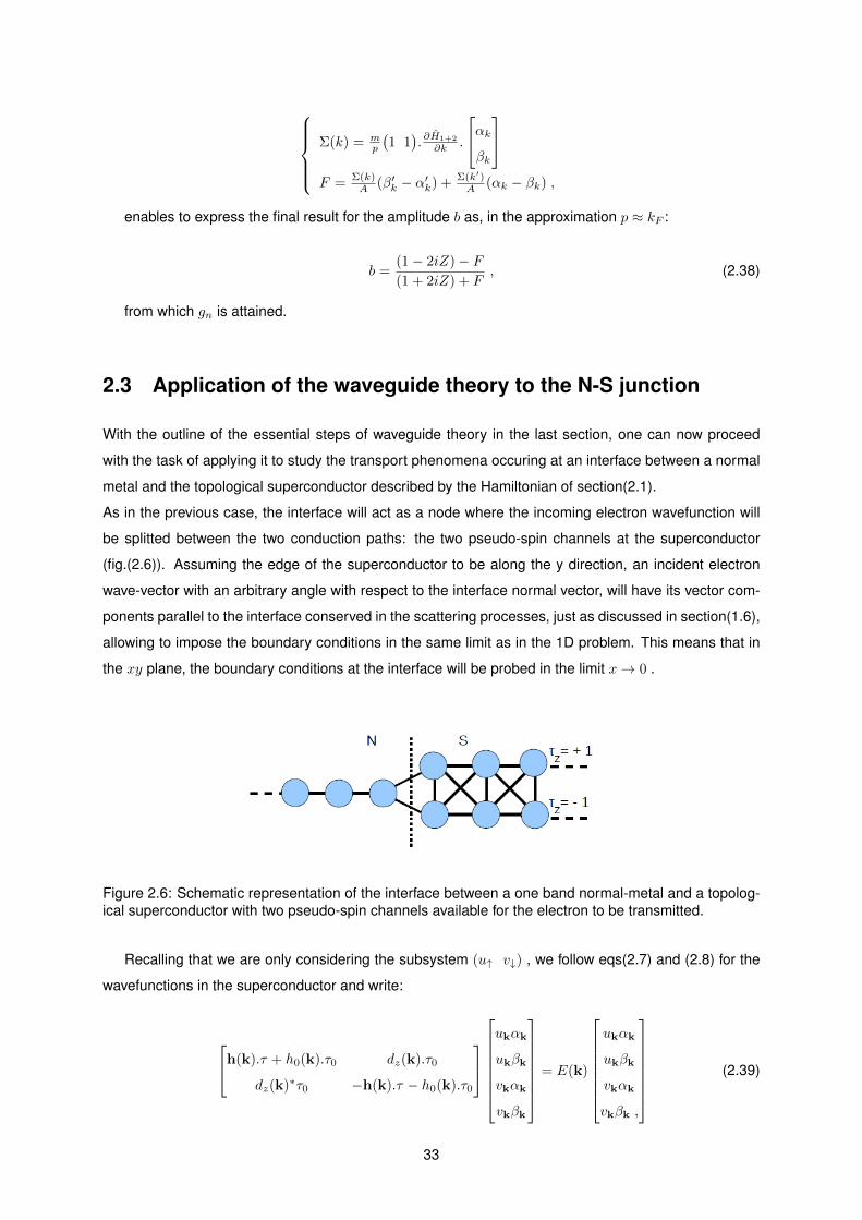
Σ(k) = m

p

(1 1).∂H1+2

∂k .

αkβk

F = Σ(k)

A (β′k − α′k) + Σ(k′)A (αk − βk) ,

enables to express the final result for the amplitude b as, in the approximation p ≈ kF :

b =(1− 2iZ)− F(1 + 2iZ) + F

, (2.38)

from which gn is attained.

2.3 Application of the waveguide theory to the N-S junction

With the outline of the essential steps of waveguide theory in the last section, one can now proceed

with the task of applying it to study the transport phenomena occuring at an interface between a normal

metal and the topological superconductor described by the Hamiltonian of section(2.1).

As in the previous case, the interface will act as a node where the incoming electron wavefunction will

be splitted between the two conduction paths: the two pseudo-spin channels at the superconductor

(fig.(2.6)). Assuming the edge of the superconductor to be along the y direction, an incident electron

wave-vector with an arbitrary angle with respect to the interface normal vector, will have its vector com-

ponents parallel to the interface conserved in the scattering processes, just as discussed in section(1.6),

allowing to impose the boundary conditions in the same limit as in the 1D problem. This means that in

the xy plane, the boundary conditions at the interface will be probed in the limit x→ 0 .

Figure 2.6: Schematic representation of the interface between a one band normal-metal and a topolog-ical superconductor with two pseudo-spin channels available for the electron to be transmitted.

Recalling that we are only considering the subsystem (u↑ v↓) , we follow eqs(2.7) and (2.8) for the

wavefunctions in the superconductor and write:

h(k).τ + h0(k).τ0 dz(k).τ0

dz(k)∗τ0 −h(k).τ − h0(k).τ0

ukαk

ukβk

vkαk

vkβk

= E(k)

ukαk

ukβk

vkαk

vkβk ,

(2.39)

33

As the y component of the wavevector is a conserved quantity, one can construct the transmited

wavefunction in the superconductor’s region as eipyyΨS , where

ΨS(x ≥ 0) = Cψk+eik+x +Dψk−e

−ik−x + Eψq+eiq+x + Fψq−e

−iq−x . (2.40)

Each ψk denotes a four-dimensional column eigenvector of the BdG matrix from eq(2.39). The

transmited excitations are superpositions of the wave-vectors k± and q± from the two Fermi-surface

pockets. Their x-component is chosen such that the group velocity is positive for an energy E above

the gap (as in fig(1.9)). For the normal-metal, which is a single-band metal, the wavefunctions are those

introduced in eq.(1.67), eipyyΨN with:

ΨN (x ≤ 0) = eip+x

1

0

+ be−ip+x

1

0

+ aeip−x

0

1

(2.41)

In the approximation where k± and q± both take the value of their respective Fermi momentum, their

determination can be achieved by finding the zeros of the electron-like energy band, which are closest

to the center of correspondent Fermi-pocket.

With both wavefunctions in each region specified, one can now proceed by applying the waveguide

boundary conditions 1 and 2 . The boundary condition which imposes the wavefunction to be single

valued at the node follows immediatly if one evaluates the wavefunctions, in each region, in the limit

x→ 0 :

uk+αk+ uk−αk− uq+αk+ uq−αq−

uk+βk+ uk−βk− uq+βk+ uq−βq−

vk+αk+ vk−αk− vq+αk+ vq−αq−

vk+βk+ vk−βk− vq+βk− vq−βq−

C

D

E

F

=

1 + b

1 + b

a

a

(2.42)

To evaluate condition 2 it is necessary to probe each member of eq(2.24):

∂ε

∂p=

pm 0

0 − pm

,with: p = −i ∂∂x⇒ ∂ε

∂pΨN =

x→0−

p+

m

1

0

− bp+

m

1

0

− ap−m

0

1

. (2.43)

∂H

∂k.ψk =

x→0+

∂(h(k).τ+h0(k).τ0)

∂ku↑ + ∂dz

∂kv↓

∂d∗z∂ku↑ − ∂(h(k).τ+h0(k).τ0)

∂kv↓

=

∂(h(k).τ+h0(k).τ0)

∂kuk

αβ

+ ∂dz∂kvk

αβ

∂d∗z∂kuk

αβ

− ∂(h(k).τ+h0(k).τ0)

∂kvk

αβ

(2.44)

Thus, the current conservation at the node can be expressed as:

1− b = CΘ(k+) +DΘ(k−) + EΘ(q+) + FΘ(q−)

a = CΦ(k+) +DΦ(k−) + EΦ(q+) + FΦ(q−) ,(2.45)

34

where Θ(k) and Φ(k) are the auxiliar functions defined as follow:

Θ(k) =m

p+(1 1).

(uk∂h(k).τ + h0(k).τ0

∂kx+ vk

∂dz(k)

∂kx

)αk

βk

. (2.46)

Φ(k) =m

p−(1 1).

(vk∂h(k).τ + h0(k).τ0

∂kx− uk

∂d∗z(k)

∂kx

)αk

βk

. (2.47)

From eq(2.42) it is possible to invert the system and attain the amplitudes C, D, E and F in terms of

a and b:

C = (1+b)Γ1+aΓ2

Λ

D = (1+b)Γ3+aΓ4

Λ

E = (1+b)Γ5+aΓ6

Λ

F = (1+b)Γ7+aΓ8

Λ

(2.48)

with: Λ =

∣∣∣∣∣∣∣∣∣∣∣∣

uk+αk+ uk−αk− uq+αk+ uq−αq−

uk+βk+ uk−βk− uq+βk+ uq−βq−

vk+αk+ vk−αk− vq+αk+ vq−αq−

vk+βk+ vk−βk− vq+βk− vq−βq−

∣∣∣∣∣∣∣∣∣∣∣∣(2.49)

The coefficients Γi are given by linear combinations of the cofactor elements Clj that form the inverse

matrix of system (2.42). For example, Γ1 = C11 + C12.

It is now explicit that the reflection and the Andreev amplitudes will become dependent on the determi-

nant of the matrix Λ. Also, one will expect, as argued in section(1.6), that when Λ→ 0 ,these amplitudes

will become independent of the barrier strength, with the transmission occuring via the localized ABS.

It is still necessary to introduce the effect of the repulsive potential at the interface. As in the last section,

the problem can be more easily addressed if the repulsive potential is slightly shifted from the node

point, thus allowing it to be treated at the normal single-band region. The only difference will be due to

the presence of the superconductor, which will require for the metal’s scattering wavefunction, both at

the right and left side of the barrier potential, to have electron and hole non-null components:

ψN (x ≤ ε) = eip+x

1

0

+ be−ip+x

1

0

+ aeip−x

0

1

(2.50)

ψN (ε < x < 0) = αeip+x

1

0

+ βe−ip+x

1

0

+ γeip−x

0

1

+ ηe−ip−x

0

1

(2.51)

Taking the same boundary conditions specified in eq(2.31), the end result in the limit ε → 0 will be

equivalent with only two extra equations, owing to the presence of hole-like excitations:

γ + η = a

γ − η = ( 2mUi~2p− + 1)a .

35

Thus, the reflection coefficient b will be affected in the same manner, with its dependence upon

the dimensionless barrier parameter Z given by eq(2.37). The Andreev reflection amplitude will also

be modified, which can be seen when imposing the waveguide matching conditions to the last set of

equations, particulary, the requirement 2 will lead to the equality:

a(1− 2ikFZ

p−) = CΦ(k+) +DΦ(k−) + EΦ(q+) + FΦ(q−) (2.52)

,

which requires, by comparison with the second equation in system(2.45), for a to be modified in this

equation as:

a→ a(1− 2ikFZ

p−) (2.53)

.

With these replacements plus eq(2.48), it is possible to rewrite the equations coming from the bound-

ary condition 2. as:

(1− b)− 2iZ kFp+ (1 + b) = 1

Λ (ζ11(1 + b) + aζ12)

a(1− 2iZ kFp− ) = 1

Λ (ζ21(1 + b) + aζ22) ,(2.54)

where ζij , (i, j) = 1, 2 are the quantities arising from the replacement of C, D, E and F in eq(2.52)

and are defined as:

ζ11 = Γ1Θ(k+) + Γ3Θ(k−) + Γ5Θ(q+) + Γ7Θ(q−)

ζ12 = Γ2Θ(k+) + Γ4Θ(k−) + Γ6Θ(q+) + Γ8Θ(q−)

ζ21 = Γ1Φ(k+) + Γ3Φ(k−) + Γ5Φ(q+) + Γ7Φ(q−)

ζ22 = Γ2Φ(k+) + Γ4Φ(k−) + Γ6Φ(q+) + Γ8Φ(q−) .

(2.55)

Solving the system of eqs(2.54), one obtains the final form for the amplitudes of normal and Andreev

reflection:

a =2ζ21Λ

(1 + 2iZ + ζ11Λ )(1− 2iZ − ζ22

Λ ) + ζ12ζ21Λ2

(2.56)

b =(1− 2iZ − ζ11

Λ )(1− 2iZ − ζ22Λ )− ζ12ζ21

Λ2

(1 + 2iZ + ζ11Λ )(1− 2iZ − ζ22

Λ ) + ζ12ζ21Λ2

(2.57)

It is then possible to calculate the differential conductance of the N-S junction, gs = 1 + |a|2 −

|b|2, although a concrete value can only be attained with the knowledge of the amplitudes uk and vk

. As already argued, such task can be accomplished using the Bogolubov equations together with the

normalization condition. Since py will be a fixed quantity and particularly because it will only take upon

the two values - 0 or π - the pairing potential will be a real function of the momentum in the x direction,

if kx (or qx ) is real. Thus, a possible solution for E ≤ ∆ is :

36

v(l+, py) = 1√2

u(l+, py) =dz(l+,py)

E−i√|dz(l+,py)|2−E2

v(l+, py)

u(l−, py) = 1√2

v(l−, py) =dz(l−,py)

E−i√|dz(l−,py)|2−E2

v(l−, py)

, (2.58)

where l = k, q . For E > ∆ :

u(l+, py) =

√1 + 1

2

√E2−|dz(l+,py)|2

E

v(l+, py) =dz(l+,py)

E+√E2−|dz(l+,py)|2

u(l+, py)

v(l−, py) =

√1 + 1

2

√E2−|dz(l−,py)|2

E

u(l−, py) =dz(l−,py)

E+√E2−|dz(l−,py)|2

v(l−, py)

. (2.59)

A final remark should be given to the case where py = π and t2 = −0.08 .For such transverse momen-

tum only one real electron pocket will be intersected, the (0, π) pocket. However, quantum waveguide

theory can still be applied if one allows the momentum of the ”missing” pocket to be complex.

2.4 Differential conductance of the N-S boundary

All the above construction can be applied to determine the behavior of the differential conductance gs as

a function of the bias voltage. Particularly, gs will be computed in two distinct choices for the Hamiltonian

parameter t2 ( t2 = +0.08 and t2 = −0.08 ) which, as mentioned before, lead the system into two distinct

phases: a trivial and a topological phase, respectively. For the transverse momentum fixed at normal

incidence, py = 0 , and considering the non-topological case, waveguide theory provides the results in

fig(2.7)-(2.9) , which account for different magnitudes of the strength barrier, Z.

Figure 2.7: Conductance gs and gn as function of the incident electron energy for t2 = +0.08 in amicroconstriction, Z=0, for a fixed transverse momentum py= 0. Calculation performed with waveguidetheory.

37

As one may see, the electron transport at zero energy-bias E → 0 is supressed, even though ex-

citations k+ and q+ are submitted to a sign-reversed pairing potential version of their correspondent

counterpart k− and q− , which might lead to expect a similiar situation as in d-wave superconductivity,

fig(1.7 b) ). Also, the observed vanishment of gs for E → 0 becomes more pronounced with the increase

of the disorder parameter Z.

Figure 2.8: Conductance gs and gn as function of the incident electron energy for t2 = +0.08 and Z=1,for a fixed transverse momentum py=0. Calculation performed with waveguide theory.

Figure 2.9: Conductance gs and gn as function of the incident electron energy for t2 = +0.08 and Z=2,for a fixed transverse momentum py= 0. Calculation performed with waveguide theory.

If one applies the generalized form of BTK theory for an anisotropic pair potential, the resulting

differential conductance will behave similar to fig(1.7 b) ), predicting an ABS at zero energy in each

38

Fermi-pocket , identifiable by the condition discussed in section(1.6) : Λ→ 0 . This condition was never

satisfied for the differential conductances attained with waveguide theory for t2 = +0.08 .

Figure 2.10: Conductance gs as function of the incident electron energy for t2 = +0.08 in a microcon-striction, Z=0, computed with BTK generalized model, for a fixed transverse momentum py=0.

With the same choice of the parameter t2 , but altering the transversed momentum to py = π ,

waveguide theory predicts the behaviour of the differential conductances in fig(2.11)-(2.13) . Similarly to

py = 0 there are no bound states and the conductivity at zero bias energy is supressed.

Figure 2.11: Conductance gs and gn as function of the incident electron energy for t2 = +0.08 and Z=0,for a fixed transverse momentum py=π. Calculation performed with waveguide theory.

One may notice the presence of peaks and valleys which occur at bias energies coinciding with the

value of the pair potential at the momentum kF and qF .

39

Figure 2.12: Conductance gs and gn as function of the incident electron energy for t2 = +0.08 and Z=1,for a fixed transverse momentum py=π. Calculation performed with waveguide theory.

Furthermore, the assymptotic behaviour of the differential conductance gs as the bias energy in-

creases is similar in all the present figures: it becomes increasingly closer to the normal conductance gn

, illustrating that the special features of the N-S junction are circumscribed to a range of energies near

the gap energy.

Figure 2.13: Conductance gs and gn as function of the incident electron energy for t2 = +0.08 and Z=2,for a fixed transverse momentum py=π. Calculation performed with waveguide theory.

For the topological phase, considering a normal incidence, py = 0 , and applying quantum waveguide

theory provides a similar qualitative picture as for t2 = +0.08 , with also zero conductance at E → 0 .

40

Figure 2.14: Conductance gs and gn as function of the incident electron energy for t2 = −0.08 and Z=0and a fixed transverse momentum py=0. Calculation performed with waveguide theory.

Figure 2.15: Conductance gs and gn as function of the incident electron energy for t2 = −0.08 and Z=1and a fixed transverse momentum py=0. Calculation performed with waveguide theory.

41

Figure 2.16: Conductance gs and gn as function of the incident electron energy for t2 = −0.08 and Z=2and a fixed transverse momentum py=0. Calculation performed with waveguide theory.

Likewise, applying the extended version of the BTK theory in this case results in the opposite predic-

tion with an enhanced flow of current occuring at zero bias and detecting the presence of an ABS which

would be a Majorana fermion, due to topology. The model also grants the same conclusion if rather

than a normal incidence, the transverse momentum is fixed at py = π. Thus BTK theory predicts the

existence of a Majorana fermion in each Fermi pocket, a contradiction with the topological properties of

the system which only allow one Majorana fermion.

Figure 2.17: Conductance gs as function of the incident electron energy for t2 = −0.08 with variousstrength barriers and a fixed transverse momentum py=π. Calculation performed using the generalizedBTK model.

42

The differential conductance attained by waveguide theory with fixed transverse momentum py = π

and t2 = −0.08, however, breaks the pattern of suppressed zero bias conductivity and meets for the first

time the criterium for ABS.

Figure 2.18: Conductance gs as function of the incident electron energy for t2 = −0.08 with variousstrength barriers and a fixed transverse momentum py=π. Calculation performed using waveguide the-ory.

One can observe that the enhanced peak located at zero energy is conserved even when the barrier

parameter increases to Z = 5 , therefore being independent of the local interface disorder, which is

exactly what one would expect for an ABS. Because the parameter choice imposes a topological phase,

the localized ABS can be identified as a Majorana fermion.

With all these considerations, it is then possible to conclude that in order to attain consistency between

the topological properties of the system and the number of ABS in each Fermi-pocket, it is necessary

that an interference effect occurs between the two traversed Fermi pockets, fixed by the momentum py.

These interference effects are correctly accounted for by waveguide theory, emphasizing the importance

of taking into account from the start the various conduction channels at a multiband superconductor,

rather than treating them independently and constructing the final differential conductance as a sum of

all separate contributions. Furthermore, when applied to a single pocket, waveguide theory proved to

attain the correct behaviour expected in the presence of ABS.

43

44

Chapter 3

Conclusions and future work

For the choice of the Hamiltonian’s parameter t2 = −0.08, the Fermi surface is composed by an odd

number of electron pockets and quantum waveguide theory allows a differential conductivity with a zero-

energy ABS located at the single pocket, which can be identified as a Majorana fermion because with

such value of t2 the system is in a topological phase with C = 1. This ABS is also present when the

differential conductance of the single-pocket is attained in the BTK framework, although the theory also

predicts an ABS in each of the other electron-pockets even when the system is non-topological. This

suggests that for the number of ABS to be reconciled with the topological properties of the system, the

two ABS states predicted by BTK theory for the pockets (0, 0) and (π, 0) should interfere destructively

when the incident electron has transverse momentum py = 0. For quantum waveguide theory this is

exactly what is observed. Thus, quantum waveguide correctly integrates the number of calculated ABS

with the topological features of the model, revealing the presence of important quantum interference

effects suppressing conductivity at zero energy bias, when two real electron pockets are transversed, a

phenomena which will not be observed if the bands are treated as separate conduction channels and

added together to form the differential conductivity at the interface.

As future work it would be interesting to study: the effect of spin-orbit interaction, by introducing a

Rabash term in the Hamiltonian. The Rabash spin-orbit term can lead to the recent discovered phe-

nomena of selective equal spin Andreev reflection [37], which consists of incident electrons, with certain

spin orientations, being reflected as holes with the same spin, at the interface between a normal-metal

and a topological superconductor; or calculate the differential conductance gs for the crossed Andreev

reflection mechanism.

45

46

Bibliography

[1] Jan Carl Budich and Bjorn Trauzettel, From adiabatic theorem of quantum mechanics to topological

states of matter, Physica Status Solidi (RRL) - Rapid Research Letters,7,109 (2013).

[2] M. Z. Hasan and C. L. Kane, Colloquium: Topological insulators, Reviews of Modern Physics, 82,

3045, (2010).

[3] B. Andrei Bernevig and Taylor L.Hughes, Topological Insulators and Topological Superconductors,

Princeton University Press (2013).

[4] Xue-Feng Wang, Yibin Hu, and Hong Guo, Robustness of the helical edge states in topological

insulators, Phys. Rev. B, 85, 241402(R) (2012).

[5] M.V.Berry and F.R.S., Quantal phase factors accompanying adiabatic changes, Proc.R.Soc.London

A, 392, 45 (1983).

[6] Alexey A. Soluyanov and David Vanderbilt, Smooth gauge for topological insulators, Phys. Rev. B,

85, 115415 (2012).

[7] Qian Niu, D.J.Thouless and Yong-Shi Wu, Quantized Hall conductance as a topological invariant,

Physical Review B, 31, 3372 (1985).

[8] Andreas P. Schnyder, Shinsei Ryu, Akira Furusaki and Andreas W.W. Ludwig, Classification of

topological insulators and superconductors in three spatial dimensions, Physical Review B, 78,

195125 (2008).

[9] Xiao-Liang Qi and Shou-Cheng Zhang, Topological insulators and superconductors, Rev. Mod.

Phys., 83, 1057 (2011).

[10] C. L. Kane and E. J. Mele, Z2 Topological Order and the Quantum Spin Hall Effect, Physical Review

Letters, 95, 146802 (2005).

[11] C. L. Kane and E. J. Mele, Quantum Spin Hall Effect in Graphene, Physical Review Letters, 95,

226801 (2005).

[12] Manfred Sigrist and Kazuo Ueda, Phenomenological theory of unconventional superconductivity,

Reviews of Modern Physics, 63, 239 (1991).

[13] P.G. De Gennes, Superconductivity of Metals and Alloys, Oxford Science Publications (2012).

47

[14] Jason Alicea, New directions in the pursuit of Majorana fermions in solid state systems, Rep. Prog.

Phys., 75, 076501 (2012).

[15] Martin Leijnse and Karsten Flensberg, Introduction to topological superconductivity and Majorana

fermions, Semiconductor Science and Technology, 27 , 124003 (2012).

[16] Shinsei Ryu, Hunting Majorana Fermions in Topological Superconductors, Journal of the Physical

Society of Japan, News Comments 11, 11 (2014).

[17] Alexei Kitaev, Unpaired Majorana fermions in quantum wires, Phys.-Usp., 44 , 131 (2001).

[18] X. Chen, C. Huan, Y. S. Hor, C.A.R.S a de Melo and Z. Jiang, Point-contact Andreev reflection

spectroscopy of candidate topological superconductor Cu0.25Bi2Se3 , arXiv:1210.6054v1 (2012).

[19] E.L.Wolf, Principles of Electron Tunneling Spectroscopy, Oxford Science Publications (2012).

[20] G. E. Blonder, M. Tinkham and T. M. Klapwijk, Transition from metallic to tunneling regimes in su-

perconducting microconstrictions: Excess current, charge imbalance and supercurrent conversion,

Physical Review B, 7, 4515 (1982).

[21] Satoshi Kashiwaya, Yukio Tanaka, Masao Koyanagi and Koji Kajimura, Theory for tunneling spec-

troscopy of anisotropic superconductors, Physical Review B, 53, 2667 (1996).

[22] Ville F. Maisi, Andreev tunneling and quasiparticle excitations in mesoscopic normal metal - super-

conductor structures, PhD thesis, Aalto University (2014).

[23] Pouyan Ghaemi, Fa Wang and Ashvin Vishwanath, Andreev Bound States as a Phase-Sensitive

Probe of the Pairing Symmetry of the Iron Pnictide Superconductors, Physical Review Letters, 102,

157002 (2009).

[24] Chia-Ren Hu, Midgap Surface States as a Novel Signature for dx2a−x2

b-Wave Superconductivity,

Physical Review Letters, 72, 1526 (1994).

[25] Guy Deutscher, Andreev–Saint-James reflections: A probe of cuprate superconductors, Reviews

of Modern Physics, 77, 109 (2005).

[26] V. Mourik, K. Zuo,S. M. Frolov, S. R. Plissard, E. P. A. M. Bakkers, L. P. Kouwenhoven, Signatures

of Majorana Fermions in Hybrid Superconductor-Semiconductor Nanowire Devices, Science, 336,

1003 (2012).

[27] Satoshi Sasaki,M. Kriener, Kouji Segawa, Keiji Yada, Yukio Tanaka, Masatoshi Sato and Yoichi

Ando, Topological Superconductivity in CuxBi2Se3 , Physical Review Letters, 107, 217001 (2011).

[28] M. A. N. Arau jo and P. D. Sacramento, Quantum waveguide theory of Andreev spectroscopy in

multiband superconductors: the case of Fe-pnictides, Physical Review B, 79, 174529 (2009).

[29] Jacob Linder and Asle Sudbø, Theory of Andreev reflection in junctions with iron-based high-Tc

superconductors, Physical Review B, 79, 020501(R) (2009).

48

[30] Jian-Bai Xia, Quantum waveguide theory for mesoscopic structures, Physical Review B, 45, 3593

(1992).

[31] M.A.N.Araujo and P. D. Sacramento, Electron transmission in normal metal/heavy-fermion super-

conductor junctions: A two-band model, Physical Review B, 77, 134519 (2008).

[32] M. Tinkham, Introduction to Superconductivity, Dover Publications (2004).

[33] Yousef Rohanizadegan, Generalization of the BTK Theory to the Case of Finite Quasiparticle Life-

times, Master’s thesis, Brock University (2013).

[34] Charles Kittel, Introduction to Solid State Physics, eighth edition, Oxford Science Publications

(2012).

[35] Yasuhiro Hatsugai, Takahiro Fukui and Hideo Aoki, Topological analysis of the quantum Hall effect

in graphene: Dirac-Fermi transition across van Hove singularities and edge versus bulk quantum

numbers, Physical Review B, 74, 205414 (2006).

[36] Takahiro Fukui, Yasuhiro Hatsugai and Hiroshi Suzuki, Chern Numbers in Discretized Brillouin

Zone: Efficient Method of Computing (Spin) Hall Conductances, J. Phys. Soc. Jpn., 74 , 1674

(2005).

[37] James J. He,T. K. Ng,Patrick A. Lee and K. T. Law, Selective Equal-Spin Andreev Reflections In-

duced by Majorana Fermions, Physical Review Letters, 112, 037001 (2014).

[38] Timothy H. Hsieh and Liang Fu, Majorana Fermions and Exotic Surface Andreev Bound States in

Topological Superconductors: Application to CuxBi2Se3 , Phys. Rev. Lett., 108, 107005 (2012).

49

50

Appendix A

Derivation of the Bogolubov equations

for a non-uniform superconductor

The Bogolubov method is a common procedure which allows the diagonalization of a Hamiltonian such

as the BCS Hamiltonian of an inhomogeneous superconductor, where spatial variations are due to a

position dependent pair potential ∆(r) or because electrons also experience an arbitrary local potential

U(r) , which may include, for example, the Hartree-Fock averaged Coulomb potential [13, 32]:

H =

∫d3r

∑α

ψ†α(r)(− 1

2m∇2 + U(r)− µ(r)

)ψα(r)− V

∫d3rψ†↑(r)ψ†↓(r)ψ↓(r)ψ↑(r) ,with: α = ↑, ↓

(A.1)

V arises from the BCS attractive two-body potential Vkk′ mediating the interaction between the elec-

trons forming a Cooper pair and is taken in the Cooper approximation:

Vkk′ =

−V for |ξk| < ~wD0 otherwise

, (A.2)

where ~wD is the Debye energy and ξk is the one-electron energy measured from the Fermi level.

The operators ψ and ψ† are the annihilation/creation operators for fermions in real space and can be

attained from the usual momentum operators by a Fourier transform operation [13]:

ψα(r) =∑k

eik.rcαk (A.3)

As in the BCS theory for homogeneous superconductors the term ψ†↑(r)ψ†↓(r)ψ↓(r)ψ↑(r) can be trans-

formed into a quadratic form by performing the mean field approximation:

ψ†↑(r)ψ†↓(r) = A

ψ↓(r)ψ↑(r) = B(A.4)

51

⇒ A.B = (〈A〉+ δA).(〈B〉+ δB) ≈ 〈A〉B + 〈B〉A− 〈A〉〈B〉 . (A.5)

Then, by defining:

∆(r) = −V 〈ψ↑(r)ψ↓(r)〉 , (A.6)

The effective Hamiltonian from eq. (A.1) can be written as:

Heff =

∫d3r

∑α

ψ†α(r)(− 1

2m∇2 + U(r)− µ(r)

)ψα(r) + ∆∗(r)ψ↓(r)ψ↑(r) + ∆(r)ψ†↑(r)ψ†↓(r) (A.7)

The Hamiltonian is now quadratic in the operators ψ and ψ† but not diagonal. However, eq(A.7) can

be diagonalized by a suitable unitary transformation in which one looks for new operators such that:

Heff = EGroud state +∑n,α

εnγ†nαγnα , (A.8)

where εn is the excitation energy of the n state. This transformation is accomplished if :

ψ↑(r) =∑n(γn↑un(r)− γ†↓v∗n(r))

ψ↓(r) =∑n(γn↓un(r) + γ†↑v

∗n(r))

. (A.9)

Taking the commutator of Heff with the new operators γ and γ† and with the spatial dependent

operators ψ and ψ† , one obtains :

[Heff , γnα] = −εmγnα (A.10)

[Heff , γ†nα] = εmγ

†nα (A.11)

[ψ↑(r), Heff ] = H0ψ↑(r) + ∆(r)ψ†↓ (A.12)

[ψ↓(r), Heff ] = H0ψ↓(r)−∆∗(r)ψ†↑ (A.13)

with H0 the one electron Hamiltonian given by H0 = − 12m∇

2 + U(r) − µ(r). Then inserting eq(A.9)

(and its adjunct form) in the above equations, and using eq(A.10) plus eq(A.11), one will attain the

coupled system of equations: εun(r) = H0un(r) + ∆(r)vn(r)

εvn(r) = −H∗0vn(r) + ∆∗(r)un(r)(A.14)

These are the Bogoliuvbov equations. Particularly, this spatially dependent form is the one used in the

BTK paper and in the limit where ∆ , µ and U are constants, the equations will admit as eigenfunctions

the momentum plane-waves, allowing to express eq(A.14) in the same form as in the original BCS

52

development for uniform superconductors.

53

Appendix B

Fukui-Hatsugai-Suzuki method for

calculating the Chern number on a

discretized Brillouin zone.

The calculations for the Chern number followed the numerical implementation of the method which is

here described [35, 36]. It will be first addressed the case where the eigenstates are non-degenerate,

as it will be useful to introduce the key steps of the method and also provide a clearer connection to the

original formula in eq(1.3). Then, the adaptation of the model for a non-Abelian Chern number will be

presented, which was the method applied to attain the results in eq(2.15 ).

The Brillouin zone will be given by the discrete set of points kµ = 2πjN , with j = 1, ..., N and µ = x, y,

connected by a link δkµ which will be a vector in the µ direction with magnitude 2πN . Defining the link

variable:

Uµ(k) =〈n(k)|n(k + δkµ)〉|〈n(k)|n(k + δkµ)〉|

, (B.1)

the Berry curvature can be constructed as:

Fxy(k) = ln(Ux(k)Uy(k + δkx)Ux(k + δky)−1Uy(k)−1) , (B.2)

which is restricted to the interval −π < −iFxy(k) ≤ π. The nth Chern number will thus be given by:

Cn =1

2iπ

∑k

Fxy(k) . (B.3)

One should note that the link variable Uµ(k) is the result of discretizing the derivative operator into

the infinitesimal difference operator:

Aµ = 〈n(k)|∂µ|n(k)〉 → 〈n(k)|n(k + δkµ)〉 − 〈n(k)|n(k)〉 . (B.4)

54

Because 〈n(k)|∂µ|n(k)〉 is a pure imaginary number (a property that follows form the normalization

condition of the Bloch eigenstates) and noticing that:

〈n(k)|∂µ|n(k)〉 → 〈n(k)|n(k + δkµ)〉 − 〈n(k)|n(k)〉 = 1− iα− 1, with α << 1 , (B.5)

⇒ 〈n(k)|n(k + δkµ)〉 = 1− iα ≈ e−iα =〈n(k)|n(k + δkµ)〉|〈n(k)|n(k + δkµ)〉|

⇒ −iα ≈ ln[ 〈n(k)|n(k + δkµ)〉|〈n(k)|n(k + δkµ)〉|

], (B.6)

Thus, the Berry connection in the discretized Brillouin zone, eq(B.4), can be expressed by the loga-

rithm of the link variable, which will provide the Berry curvature given by eq(B.2) if one also applies the

discretized version of the derivative operator to the link variable.

In the case where there exists multiple energy bands bellow the Fermi energy, the generalization

of the method to accommodate the mixing between bands follows in close resemblance to the non-

degenerated case with the only change falling into the link variable:

Uµ =det(φµ)

|det(φµ)|. (B.7)

Here φµ is a matrix formed by the elements (φµ)ij = 〈ni(k)|nj(k + δkµ)〉 , with 0 ≤ i, j ≤ n and where

n is the number of bands bellow the Fermi level. The Berry connection and the Chern number can then

be obtained following the same expressions as in the non-degenerate case: eq( B.2) and eq( B.3 ).

55

Appendix C

The problem of finding a consistent

Gauge in a two-band model

The Bloch Hamiltonian for a two-band model is given by h(k).σ, for which it is possible to express the

eigenstates in spherical coordinates as:

|ψ−〉 =

sin( θ2 )

−eiφcos( θ2 )

(C.1)

|ψ+〉 =

cos( θ2 )

eiφsin( θ2 )

. (C.2)

Restricting our attention in the |ψ−〉 state, if we compute it for θ = 0

|ψ−〉 →

0

−eiφ

(C.3)

we see that the eigenstate depends on the azimuthal angle φ, which is ill-defined at θ = 0 because

if φ is either 0 or π, the correspondent point in space will be exactly the same, but for |ψ−〉 this implies

jumping from (0,-1) to (0,1). Thus, the eigenstate is not single-valued over the full S2 sphere. We can

try to find another gauge in which this ”anomaly” point is no longer present. For example, we could try:

|ψ−〉 → e−iφ|ψ−〉 = |ψ′−〉 . (C.4)

Now the eigenstate is well defined for θ = 0, but it will have the same problem for θ = π and hence, there

is no gauge for which |ψ−〉 will be well defined for both θ = 0 and θ = π [3].

In the vector h space, the sphere can be constructed by the orthogonal unit vectors:

hz =hz|h|

= cos(θ), hx =hx|h|

= sin(θ)cos(φ), hy =hy|h|

= sin(θ)sin(φ) , (C.5)

from which we can see that if hz(k) is positive at all points of the Brillouin zone, cos(θ) > 0 ⇒

56

θ ∈ [0, π2 ] and hence the second gauge choice, |ψ′−〉, will guarantee a global well-defined eigenvector,

because θ will never visit the south pole (θ = π). Likewise, if hz(k) is always negative, θ never reaches

the north pole and the first gauge will provide a well define eigenstate over the entire Brillouin zone.

Nevertheless, if we can define a global gauge, the Chern number will be zero (as discussed in the

first chapter). Hence, it is when hz(k) changes sign and visits both the north and south pole of the S2

sphere, which will be when it is impossible to define a global, continuous and smooth gauge over the

entire Brillouin zone, that a topologically nontrivial phase will exist [3].

57

58