Embed Size (px)
Citation preview
The Effect of Price and Non-Price Conservation Programs on Residential Water Demand
Serhat Asci and Tatiana Borisova
Authors are, respectively, Postdoctoral Associate, [email protected], and Assistant Professor, [email protected], in the Food and Resource Economics
Department, University of Florida.
Selected Paper prepared for presentation at the Agricultural & Applied Economics Association’s 2014 AAEA Annual Meeting, Minneapolis, MN, July 27-29, 2014.
Copyright 2014 by Serhat Asci and Tatiana Borisova. All rights reserved. Readers may
make verbatim copies of this document for non-commercial purposes by any means,
provided this copyright notice appears on all such copies.
1
The Effect of Price and Non-Price Conservation Programs on Residential Water Demand
Abstract. The study examines effectiveness of price- and non-price residential water
demand management programs. Household-level water use data for Alachua County, Florida,
were analyzed using three methods: IV, 2SLS, and 3SLS. Residential water demand is
examined separately for households with combined water meters, as well as separate indoor
and outdoor irrigation water meters. Preliminary results show that the price-base program
(i.e., inclining block rate pricing) and non-price programs (i.e., residential irrigation
restrictions with an enforcement component) have a significant effect on monthly household
water use.
Acknowledgements. We appreciate cooperation with Stacie Greco, Alachua County
Environmental Protection Division, and Jennifer McElroy and Amy Carpus, Gainesville
Regional Utilities, who shared with us the household water use data and information related to
the enforcement of residential irrigation restrictions.
Introduction
Nationwide, 44.2 billion gallons of freshwater per day is withdrawn for public water
supply, with California, Florida, New York, and Texas accounting for 37 percent of this
volume (Kenney et al. 2009). Residential water conservation is one of the primary strategies
to cope with the challenge of meeting water demands given continuous population growth,
limited freshwater resources, lack of opportunities for water transfers among water use sectors
(such transfers between agriculture and urban sectors), and potential impacts of climate
change (Ozan and Alsharif 2013, Olmstead and Stavins 2007). To encourage water
conservation, state and local agencies and water utility companies use a variety of price-based
2
water demand management strategies, including inclining block pricing schemes (i.e.,
increasing per-unit water prices depending on water use volumes). Non-price demand
management programs are also used widely, including residential irrigation restrictions, toilet
replacement programs, and outreach programs. Existing economic studies have examined
reduction in residential water use given inclining block pricing schemes implemented
simultaneously with non-price programs. However, the appropriate methodology for
modelling residential water demand and estimating the effectiveness of price and non-price
demand management programs are still in discussion. In this paper, we use panel dataset of
household-level water use in Alachua County, Florida, and examine effectiveness of two
demand management programs: inclining block price structure (i.e., price-based program) and
residential irrigation restrictions with an inspection component (i.e., non-price program).
Implications for selecting a mix of residential water demand management programs by local
agencies are discussed.
Residential Water Demand Management
Population, household and property characteristics, climatic factors, and price and non-
price demand management programs implemented by government agencies are the principal
factors influencing residential water demand (Young, 1973, Olmstead et. al. 2007,
House‐Peters and Chang, 2011). The nature of water suggests that there is no substitute for it.
However, residential water use categories can still be classified into non-discretionary (mostly
indoor water use, such as drinking and sanitation) and discretionary (most of the outdoor
water use, such as residential irrigation). In California, Florida, Texas, and other western and
southern states with hot climates, residential irrigation accounts for one third to one half of the
total residential water use (Hermitte, 2012; Friedman et al., 2013; Southwest Florida Water
Management District, undated; Arizona Department of Water Resources, 2014). Government
3
agencies and water utility companies employ both price- and non-price programs to
encourage reduction in discretionary residential irrigation (Billing and Agthe, 1980).
Olmstead and Stavins (2007) show that for a specific water conservation goal, price-
based programs (i.e., increase in price) are generally more cost-effective than non-price
programs (such as restrictions on water use). Price-based strategies allow households the
freedom to decide what changes to make in response to price increases. Households can use
their privately-held information to make the least-cost adjustments in response to price
change, minimizing their private costs of water use reduction. In addition, price-based
programs allow for least-cost re-allocation of water among households, when households with
lower value for water cut their water use to a greater extent than the households with higher
value for water. Price-based program also encourage water conservation without jeopardizing
revenue collection goals for utility companies. Note that the effect of a price-based program
depends on the slope of the water demand function, and the slope in turn depends on the
household characteristics, seasonal weather conditions, and other factors. Given that state
agencies and utility companies usually have limited information about household water
demand functions, they may not be able to accurately predict the change in the water use in
response to price-based strategies.
In contrast to price-based programs, non-price programs directly limit specific
residential water use categories. For example, agencies and utility companies around US rely
on irrigation restrictions that limit the number of days per week (and/or the hours during a
day) when residential irrigation is allowed. Such programs leave households limited freedom
to choose what low-value activities to give up to conserve water. In addition, since agencies
and utility companies have limited information about household-specific water demands, the
same limits on water use are usually set for all households. Such uniform limits impose high
costs on the households that value highly the activities requiring residential irrigation. In
4
contrast, the households with low values for such activities can give up more water use than it
is required by the restrictions, and they can do that at low costs. In other words, such
programs restrict re-allocation of water among activities within the households, as well as
reallocation of water among the households, increasing the total costs of water conservation.
In theory, an advantage of water use restrictions is the ability for the agencies and water
utilities to predict water use reductions. However, in practice, the restriction programs often
lack monitoring and enforcement component, and hence, the water use levels and the water
conservation resulting from the programs remain uncertain (Olmstead and Stavins 2007).
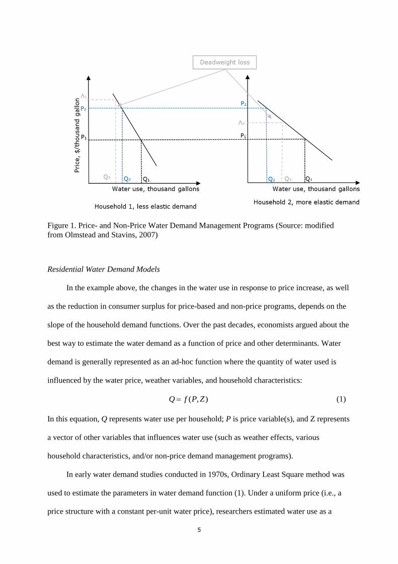
The effects on water use of price-based and non-price demand management programs
are illustrated on figure 1. Initial levels of water use for the two households is denoted by Q1.
Since households 1 have less elastic demand, the change in price from P1 to P2 does not
induce significant water use reductions for that household (as compared with household 2).
Such price-based program will result in reduction in total water use by (where
. Although households use
different volumes of water, their marginal value of water is the same and equal to the price.
Alternatively the same water conservation target can be achieved by requiring both
households to reduce water use to the same level Q3 (e.g., by imposing irrigation restrictions).
Resulting marginal value of water for household 1 will be higher than that for household 2
(compare Λ1 and Λ2), and hence, the households would be better off by “trading” water
allocations between each other (Olmstead and Stavins, 2007).
5
Figure 1. Price- and Non-Price Water Demand Management Programs (Source: modified
from Olmstead and Stavins, 2007)
Residential Water Demand Models
In the example above, the changes in the water use in response to price increase, as well
as the reduction in consumer surplus for price-based and non-price programs, depends on the
slope of the household demand functions. Over the past decades, economists argued about the
best way to estimate the water demand as a function of price and other determinants. Water
demand is generally represented as an ad-hoc function where the quantity of water used is
influenced by the water price, weather variables, and household characteristics:
),( ZPfQ (1)
In this equation, Q represents water use per household; P is price variable(s), and Z represents
a vector of other variables that influences water use (such as weather effects, various
household characteristics, and/or non-price demand management programs).
In early water demand studies conducted in 1970s, Ordinary Least Square method was
used to estimate the parameters in water demand function (1). Under a uniform price (i.e., a
price structure with a constant per-unit water price), researchers estimated water use as a
6
function of average prices and rainfall (inches) given time series data of aggregate water use
(Young, 1973), or as a function of average prices, rainfall, and household characteristics for
cross-sectional data. For instance, Foster and Beattie (1979) set the function as
),,,( NRYPfQ , where Q is the quantity of water demanded per household, P is average
water price per cubic feet, Y is median household income, R is the precipitation in inches, and
N is average number of residents per meter of living area in a house. Under block rate pricing
(with inclining per-unit water prices), Taylor (1975) proposed to include both marginal and
average prices as explanatory variables. In turn, Nordin (1976) proposed to include a
difference variable instead of average prices. The difference variable (also referred to as “rate
structure premium”) is defined as the total bill minus the product of marginal price and total
water use. The difference variable was proposed to eliminate the upward bias in price
elasticity estimates based on the marginal price only.
Although early water demand elasticity estimates that relied on OLS were lately
criticized for biased results (attributed to the endogeneity of price variables given increasing
block pricing), these elasticity estimates still provide a baseline for the later studies. The
meta-analysis of early water demand analysis showed the price elasticities from -1.24 to 0.01
(and income elasticities from 0.00 to 1.03) (Wong 1972).
The studies conducted in 1980s and 1990s extensively used panel data and instrumental
variable (IV) technique, which was first applied to the water demand analysis by Agthe and
Billing (1986a; 1986b) and Nieswiadomy and Molina (1989). Specifically, Agthe and Billing
(1986) introduced IV procedure to the demand model specified as ),,,( YWRPMPfQ
where Q is average household monthly water consumption; MP marginal price in cents; RP
rate structure premium; W evapotranspiration minus rainfall in inches; Y personal income per
household in the study area in dollars per time period. Instrumental variables for RP and MP
include the lagged values of all endogenous and exogenous variables in the system. All price
7
and income variables were adjusted for inflation using Consumer Price Index. This method
was further improved by using different IVs and 2- and 3-stage least squares techniques
(Nieswiadomy and Molina 1991; Dalhuisan et al. 2003).
An alternative method for modeling water demand decision under inclining block
pricing was introduced by Hewitt and Hanemann (1995) and Pint (1999). Researchers argued
that consumers face a two-stage choice: first, the customers choose the price block for water
use, and then they choose the quantity of water consumed within the block. To model such
choices, the researchers introduced discrete choice (D/C) model that uses logarithmic demand
function
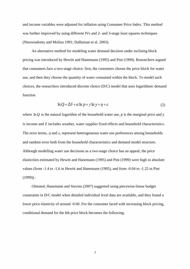
ypZQ lnlnln (2)
where Qln is the natural logarithm of the household water use, p is the marginal price and y
is income and Z includes weather, water supplier fixed effects and household characteristics.
The error terms, and , represent heterogeneous water use preferences among households
and random error both from the household characteristics and demand model structure.
Although modelling water use decisions as a two-stage choice has an appeal, the price
elasticities estimated by Hewitt and Hanemann (1995) and Pint (1999) were high in absolute
values (from -1.4 to -1.6 in Hewitt and Hanemann (1995), and from -0.04 to -1.25 in Pint
(1999)) .
Olmsted, Hanemann and Stavins (2007) suggested using piecewise-linear budget
constraints in D/C model when detailed individual level data are available, and they found a
lower price elasticity of around -0.60. For the consumer faced with increasing block pricing,
conditional demand for the kth price block becomes the following:
8
),,;~,,(lnln
),,;~,,(ln
),,;~,,(lnln),,;~,,(lnln
ln
...
),,;~,,(lnln),,;~,,(lnln
ln
),,;~,,(lnln
),,;~,,(ln
ln
*
1
*
*
111
*
11
1
22
*
2111
*
11
1
11
*
11
11
*
1
KKKK
KKK
KKKKKKKK
K
ypZqqif
ypZq
ypZqqypZqqif
q
ypZqqypZqqif
q
ypZqqif
ypZq
q (3)
where each price block is depicted by pk, optimal consumption on block k is
),,;~,,(ln * kkk ypZq , log of consumption on the kink k is kqln , and , and are
parameters to be estimated. Moreover, new income variable, ky~ , can be calculated based on
the block the consumer is on and using the following difference term:
1
1
)(
01
1
1
kif
kif
qppdk
j
kjjk
(4)
and kk dyy ~ is the income plus the difference term. An advantage of this model is the
ability to estimate both conditional elasticities for a particular consumption block choice
(using a simultaneous equations model) and unconditional elasticities for the consumption on
any block (using a maximum likelihood method). This method also allows modeling
responses to demand shocks due to significant price increases for high water use levels, since
the choice of consumption on high price blocks is modeled explicitly for high water users.
However, D/C method requires water use observations given a wide range of prices, and
hence it is not appropriate for modeling water demand of the households served by a single
water provider and given relatively narrow range of (or constant) prices. The D/C model is
9
also based on the assumption that households are aware of pricing structure, and that
assumption may not always reflect the reality.
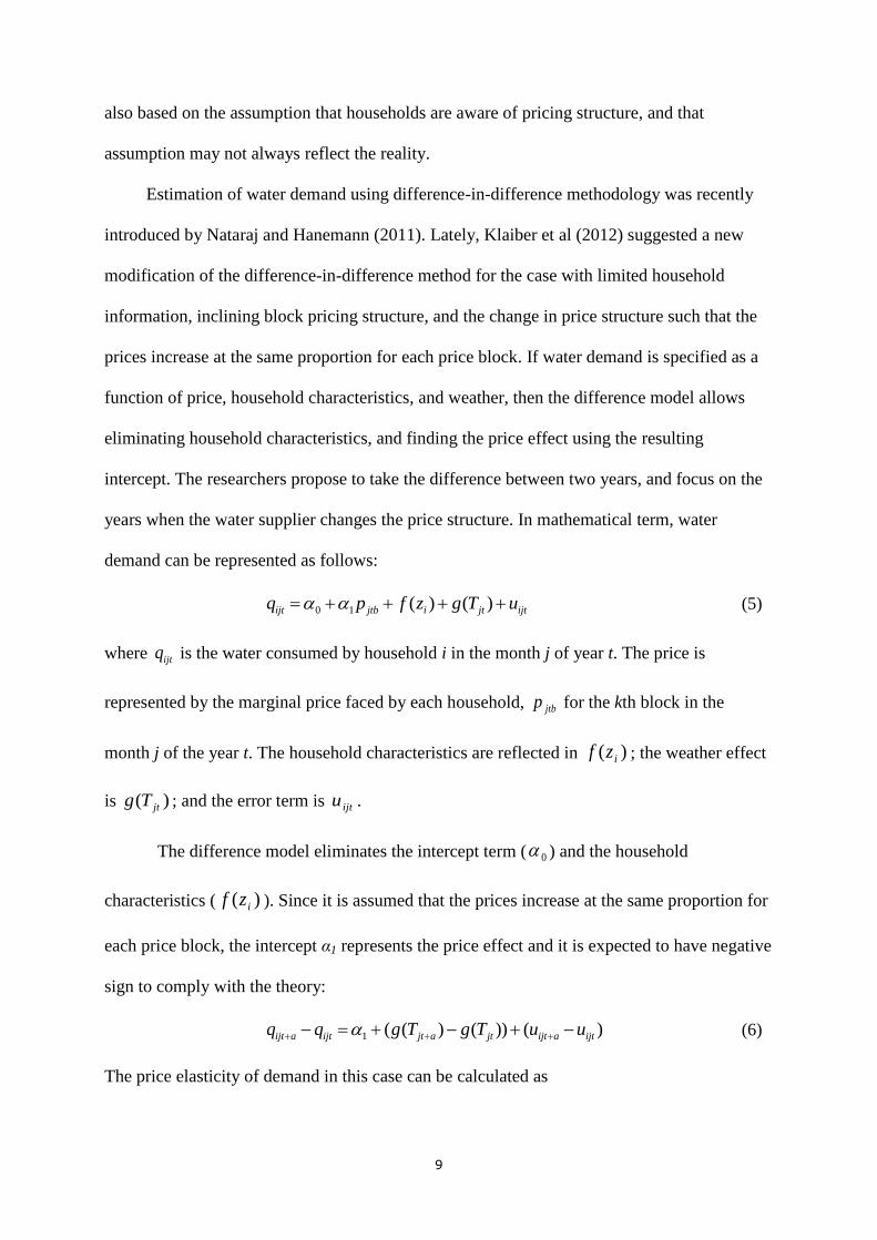
Estimation of water demand using difference-in-difference methodology was recently
introduced by Nataraj and Hanemann (2011). Lately, Klaiber et al (2012) suggested a new
modification of the difference-in-difference method for the case with limited household
information, inclining block pricing structure, and the change in price structure such that the
prices increase at the same proportion for each price block. If water demand is specified as a
function of price, household characteristics, and weather, then the difference model allows
eliminating household characteristics, and finding the price effect using the resulting
intercept. The researchers propose to take the difference between two years, and focus on the
years when the water supplier changes the price structure. In mathematical term, water
demand can be represented as follows:
ijtjtijtbijt uTgzfpq )()(10 (5)
where ijtq is the water consumed by household i in the month j of year t. The price is
represented by the marginal price faced by each household, jtbp for the kth block in the
month j of the year t. The household characteristics are reflected in )( izf ; the weather effect
is )( jtTg ; and the error term is ijtu .
The difference model eliminates the intercept term ( 0 ) and the household
characteristics ( )( izf ). Since it is assumed that the prices increase at the same proportion for
each price block, the intercept α1 represents the price effect and it is expected to have negative
sign to comply with the theory:
)())()((1 ijtaijtjtajtijtaijt uuTgTgqq (6)
The price elasticity of demand in this case can be calculated as
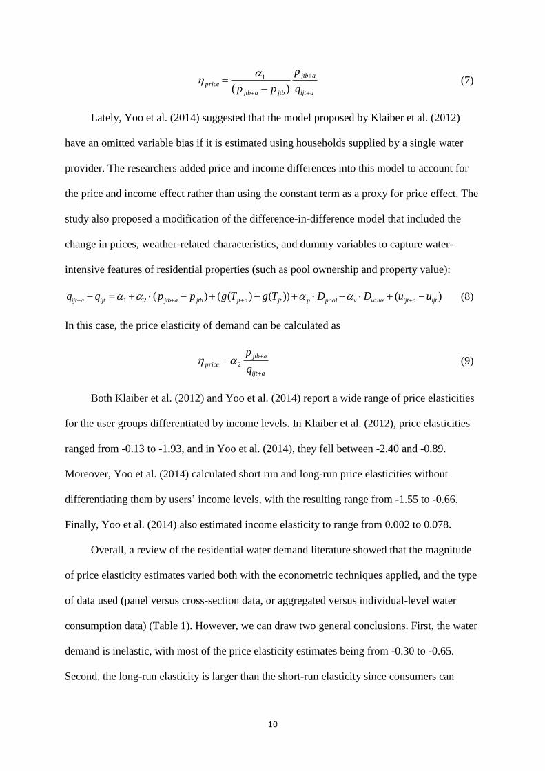
10
aijt
ajtb
jtbajtb
priceq
p
pp
)(
1 (7)
Lately, Yoo et al. (2014) suggested that the model proposed by Klaiber et al. (2012)
have an omitted variable bias if it is estimated using households supplied by a single water
provider. The researchers added price and income differences into this model to account for
the price and income effect rather than using the constant term as a proxy for price effect. The
study also proposed a modification of the difference-in-difference model that included the
change in prices, weather-related characteristics, and dummy variables to capture water-
intensive features of residential properties (such as pool ownership and property value):
)())()(()(21 ijtaijtvaluevpoolpjtajtjtbajtbijtaijt uuDDTgTgppqq (8)
In this case, the price elasticity of demand can be calculated as
aijt
ajtb
priceq
p
2 (9)
Both Klaiber et al. (2012) and Yoo et al. (2014) report a wide range of price elasticities
for the user groups differentiated by income levels. In Klaiber et al. (2012), price elasticities
ranged from -0.13 to -1.93, and in Yoo et al. (2014), they fell between -2.40 and -0.89.
Moreover, Yoo et al. (2014) calculated short run and long-run price elasticities without
differentiating them by users’ income levels, with the resulting range from -1.55 to -0.66.
Finally, Yoo et al. (2014) also estimated income elasticity to range from 0.002 to 0.078.
Overall, a review of the residential water demand literature showed that the magnitude
of price elasticity estimates varied both with the econometric techniques applied, and the type
of data used (panel versus cross-section data, or aggregated versus individual-level water
consumption data) (Table 1). However, we can draw two general conclusions. First, the water
demand is inelastic, with most of the price elasticity estimates being from -0.30 to -0.65.
Second, the long-run elasticity is larger than the short-run elasticity since consumers can
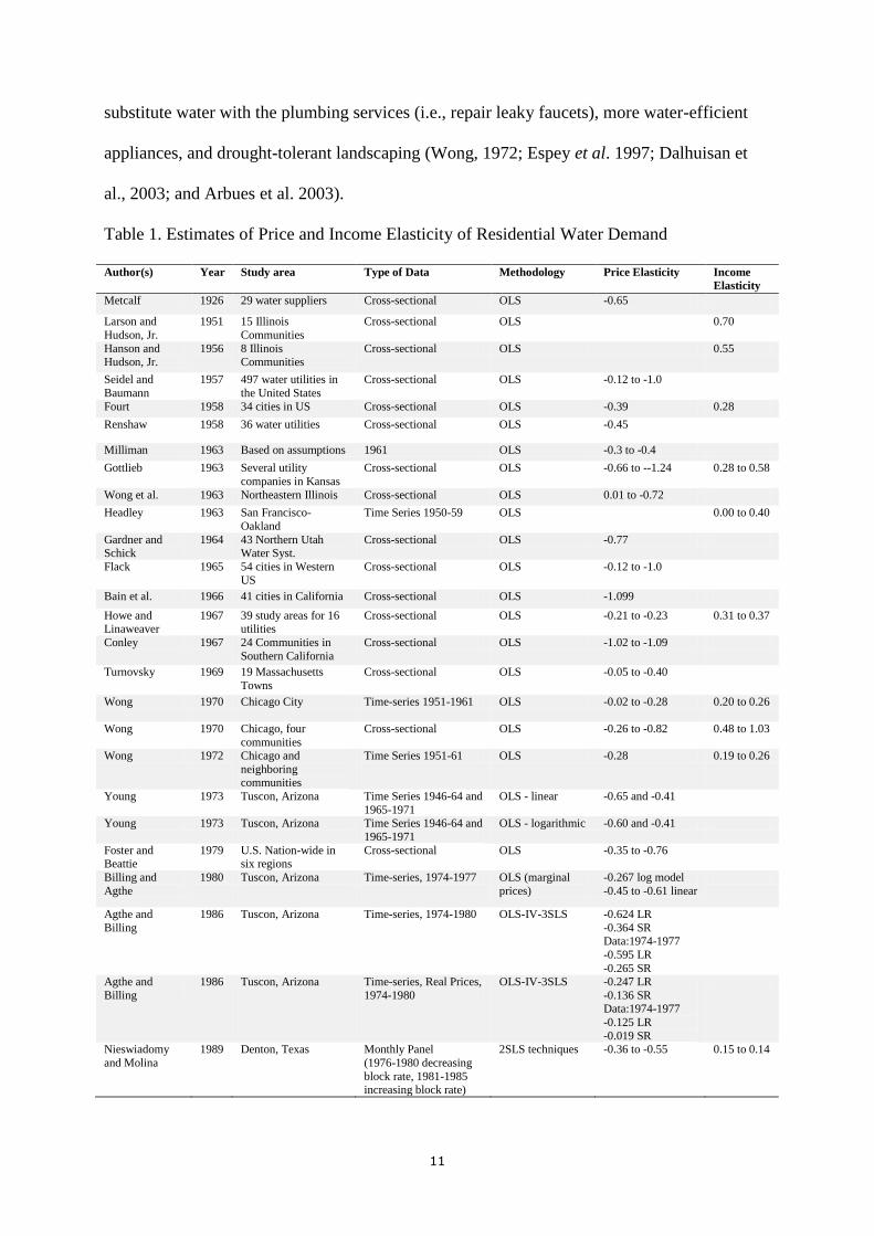
11
substitute water with the plumbing services (i.e., repair leaky faucets), more water-efficient
appliances, and drought-tolerant landscaping (Wong, 1972; Espey et al. 1997; Dalhuisan et
al., 2003; and Arbues et al. 2003).
Table 1. Estimates of Price and Income Elasticity of Residential Water Demand
Author(s) Year Study area Type of Data Methodology Price Elasticity Income
Elasticity
Metcalf 1926 29 water suppliers Cross-sectional OLS -0.65
Larson and
Hudson, Jr.
1951 15 Illinois
Communities
Cross-sectional OLS 0.70
Hanson and Hudson, Jr.
1956 8 Illinois Communities
Cross-sectional OLS 0.55
Seidel and
Baumann
1957 497 water utilities in
the United States
Cross-sectional OLS -0.12 to -1.0
Fourt 1958 34 cities in US Cross-sectional OLS -0.39 0.28
Renshaw 1958 36 water utilities Cross-sectional OLS -0.45
Milliman 1963 Based on assumptions 1961 OLS -0.3 to -0.4
Gottlieb 1963 Several utility
companies in Kansas
Cross-sectional OLS -0.66 to --1.24 0.28 to 0.58
Wong et al. 1963 Northeastern Illinois Cross-sectional OLS 0.01 to -0.72
Headley 1963 San Francisco-
Oakland
Time Series 1950-59 OLS 0.00 to 0.40
Gardner and Schick
1964 43 Northern Utah Water Syst.
Cross-sectional OLS -0.77
Flack 1965 54 cities in Western
US
Cross-sectional OLS -0.12 to -1.0
Bain et al. 1966 41 cities in California Cross-sectional OLS -1.099
Howe and Linaweaver
1967 39 study areas for 16 utilities
Cross-sectional OLS -0.21 to -0.23 0.31 to 0.37
Conley 1967 24 Communities in
Southern California
Cross-sectional OLS -1.02 to -1.09
Turnovsky 1969 19 Massachusetts
Towns
Cross-sectional OLS -0.05 to -0.40
Wong 1970 Chicago City Time-series 1951-1961 OLS -0.02 to -0.28 0.20 to 0.26
Wong 1970 Chicago, four
communities
Cross-sectional OLS -0.26 to -0.82 0.48 to 1.03
Wong 1972 Chicago and
neighboring communities
Time Series 1951-61 OLS -0.28 0.19 to 0.26
Young 1973 Tuscon, Arizona Time Series 1946-64 and
1965-1971
OLS - linear -0.65 and -0.41
Young 1973 Tuscon, Arizona Time Series 1946-64 and
1965-1971
OLS - logarithmic -0.60 and -0.41
Foster and Beattie
1979 U.S. Nation-wide in six regions
Cross-sectional OLS -0.35 to -0.76
Billing and
Agthe
1980 Tuscon, Arizona Time-series, 1974-1977 OLS (marginal
prices)
-0.267 log model
-0.45 to -0.61 linear
Agthe and
Billing
1986 Tuscon, Arizona Time-series, 1974-1980 OLS-IV-3SLS -0.624 LR
-0.364 SR Data:1974-1977
-0.595 LR
-0.265 SR
Agthe and
Billing
1986 Tuscon, Arizona Time-series, Real Prices,
1974-1980
OLS-IV-3SLS -0.247 LR
-0.136 SR Data:1974-1977
-0.125 LR
-0.019 SR
Nieswiadomy
and Molina
1989 Denton, Texas
Monthly Panel
(1976-1980 decreasing
block rate, 1981-1985 increasing block rate)
2SLS techniques
-0.36 to -0.55 0.15 to 0.14
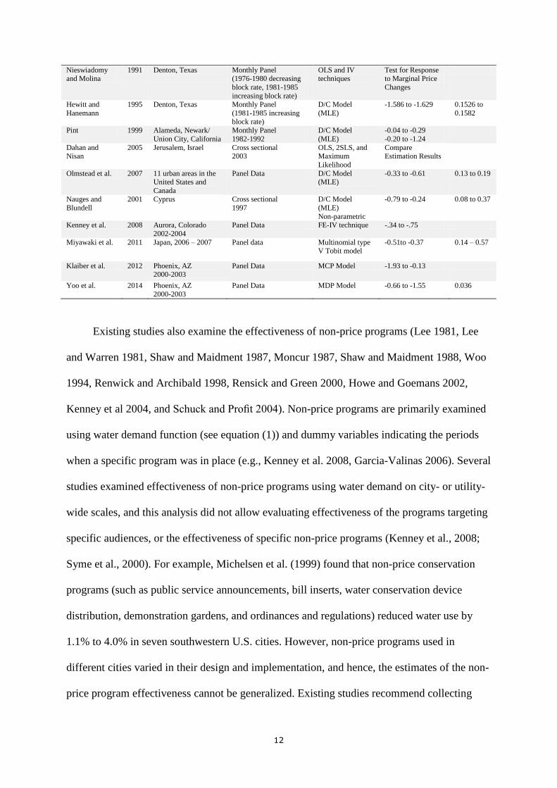
12
Nieswiadomy and Molina
1991 Denton, Texas
Monthly Panel (1976-1980 decreasing
block rate, 1981-1985
increasing block rate)
OLS and IV techniques
Test for Response to Marginal Price
Changes
Hewitt and
Hanemann
1995 Denton, Texas
Monthly Panel
(1981-1985 increasing
block rate)
D/C Model
(MLE)
-1.586 to -1.629 0.1526 to
0.1582
Pint 1999 Alameda, Newark/
Union City, California
Monthly Panel
1982-1992
D/C Model
(MLE)
-0.04 to -0.29
-0.20 to -1.24
Dahan and Nisan
2005 Jerusalem, Israel Cross sectional 2003
OLS, 2SLS, and Maximum
Likelihood
Compare Estimation Results
Olmstead et al. 2007 11 urban areas in the United States and
Canada
Panel Data D/C Model (MLE)
-0.33 to -0.61 0.13 to 0.19
Nauges and
Blundell
2001 Cyprus
Cross sectional
1997
D/C Model
(MLE)
Non-parametric
-0.79 to -0.24 0.08 to 0.37
Kenney et al. 2008 Aurora, Colorado
2002-2004
Panel Data FE-IV technique -.34 to -.75
Miyawaki et al. 2011 Japan, 2006 – 2007 Panel data Multinomial type V Tobit model
-0.51to -0.37 0.14 – 0.57
Klaiber et al. 2012 Phoenix, AZ 2000-2003
Panel Data MCP Model -1.93 to -0.13
Yoo et al. 2014 Phoenix, AZ
2000-2003
Panel Data MDP Model -0.66 to -1.55 0.036
Existing studies also examine the effectiveness of non-price programs (Lee 1981, Lee
and Warren 1981, Shaw and Maidment 1987, Moncur 1987, Shaw and Maidment 1988, Woo
1994, Renwick and Archibald 1998, Rensick and Green 2000, Howe and Goemans 2002,
Kenney et al 2004, and Schuck and Profit 2004). Non-price programs are primarily examined
using water demand function (see equation (1)) and dummy variables indicating the periods
when a specific program was in place (e.g., Kenney et al. 2008, Garcia-Valinas 2006). Several
studies examined effectiveness of non-price programs using water demand on city- or utility-
wide scales, and this analysis did not allow evaluating effectiveness of the programs targeting
specific audiences, or the effectiveness of specific non-price programs (Kenney et al., 2008;
Syme et al., 2000). For example, Michelsen et al. (1999) found that non-price conservation
programs (such as public service announcements, bill inserts, water conservation device
distribution, demonstration gardens, and ordinances and regulations) reduced water use by
1.1% to 4.0% in seven southwestern U.S. cities. However, non-price programs used in
different cities varied in their design and implementation, and hence, the estimates of the non-
price program effectiveness cannot be generalized. Existing studies recommend collecting
13
individual-level water use data and detailed and consistent information about non-price
programs to assess the effectiveness of individual non-price programs (Borisova and Useche
2013).
A growing number of economic studies examines the effectiveness of non-price
programs by explicitly modelling household utility from water use activities. For example,
Brennan et al. (2007) examine welfare impact of watering restrictions implemented in
Australia. The authors developed a household production model of optimal customer choice
between leisure and lawn quality. In Australia, watering restrictions ban sprinkler irrigation
only while irrigation through hand-held hose is allowed. Hence, households have a choice to
substitute leisure time and lawn quality (with lawn quality maintained by hand-watering). The
study showed that depending on the households’ preferences for “greenness” of the lawn and
households’ time costs, 2-day per week watering restrictions can result in 0% to 36%
reduction in water use (with high water use reduction predicted for households with high costs
of leisure time). Such explicit modelling of household utility for water use activity provides
strong theoretical background for the analysis of alternative demand management programs.
However, information about household preferences is largely unavailable, and as a result,
such method requires making assumptions about preferences for lawn characteristics and time
allocation for a “typical” water user. To avoid making strong assumptions, in this study, we
analyze effectiveness of non-price programs using monthly water, ad-hoc demand function
(1), and dummy variables indicating the periods when water use restrictions (along with the
inspection and enforcement components) were imposed.
Data
In this paper, we examine the effectiveness of price and non-price water demand
management programs, using an example of Alachua County in the north-central Florida.
14
Similar to other local governments in Florida and other states in US, Alachua County relies on
mandatory irrigation restrictions to encourage residential conservation. Residential landscape
irrigation is prohibited between 10 am and 4 pm, and is limited to once a week during Eastern
Standard Time period (winter months), and twice a week during Daylight Savings Time
(summer months). In addition, irrigation time period should be limited to one hour per zone
per irrigation day (or to ¾ inch). Exceptions are allowed for micro-irrigation systems, new
landscapes (for 60 days after planting), hand-held watering with an automatic shut-off valve,
and reclaimed water use.
Alachua County monitors compliance with irrigation restrictions by visiting high water
use neighborhoods outside of the allowed irrigation time period. Households that are
identified as non-complying with irrigation restrictions receive warning letters with
information about potential citations and fines for non-compliance. The residential inspection
program was initiated in May 2011, and in May 2011 – May 2013, roughly 800 potential
violations were identified and were sent warning letters.
Gainesville Regional Utilities (GRU) is the primary water provider for Gainesville and
surrounding areas in Alachua County. GRU employs three-block inclining price structure,
which changes every year to account for inflation and to encourage water conservation. The
water rates are effective starting from October of each year (e.g., 2012-2013 year starts in
October 2012 and ends in September 2013). For example, for 2007-2008 year, GRU used
customer charge of $5.35/month, and the inclining rates were $1.56 per thousand gallons for
the first price block (first 9 thousand gallons), $2.82 per thousand gallons for the second price
block (10 – 24 thousand gallons), and $4.93 per thousand gallons for the third block (over 25
thousand gallons). For those on separate irrigation meter, irrigation use was charged at $2.82
per thousand gallons for the first 15 thousand gallons, and $4.93 per thousand gallons for the
use over 15 thousand gallons (in addition to $5.35 monthly customer charge).
15
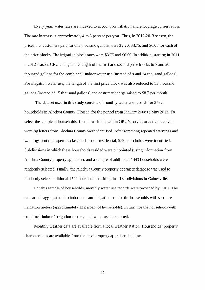
Every year, water rates are indexed to account for inflation and encourage conservation.
The rate increase is approximately 4 to 8 percent per year. Thus, in 2012-2013 season, the
prices that customers paid for one thousand gallons were $2.20, $3.75, and $6.00 for each of
the price blocks. The irrigation block rates were $3.75 and $6.00. In addition, starting in 2011
– 2012 season, GRU changed the length of the first and second price blocks to 7 and 20
thousand gallons for the combined / indoor water use (instead of 9 and 24 thousand gallons).
For irrigation water use, the length of the first price block was also reduced to 13 thousand
gallons (instead of 15 thousand gallons) and costumer charge raised to $8.7 per month.
The dataset used in this study consists of monthly water use records for 3592
households in Alachua County, Florida, for the period from January 2008 to May 2013. To
select the sample of households, first, households within GRU’s service area that received
warning letters from Alachua County were identified. After removing repeated warnings and
warnings sent to properties classified as non-residential, 559 households were identified.
Subdivisions in which these households resided were pinpointed (using information from
Alachua County property appraiser), and a sample of additional 1443 households were
randomly selected. Finally, the Alachua County property appraiser database was used to
randomly select additional 1590 households residing in all subdivisions in Gainesville.
For this sample of households, monthly water use records were provided by GRU. The
data are disaggregated into indoor use and irrigation use for the households with separate
irrigation meters (approximately 12 percent of households). In turn, for the households with
combined indoor / irrigation meters, total water use is reported.
Monthly weather data are available from a local weather station. Households’ property
characteristics are available from the local property appraiser database.
16
Methodology
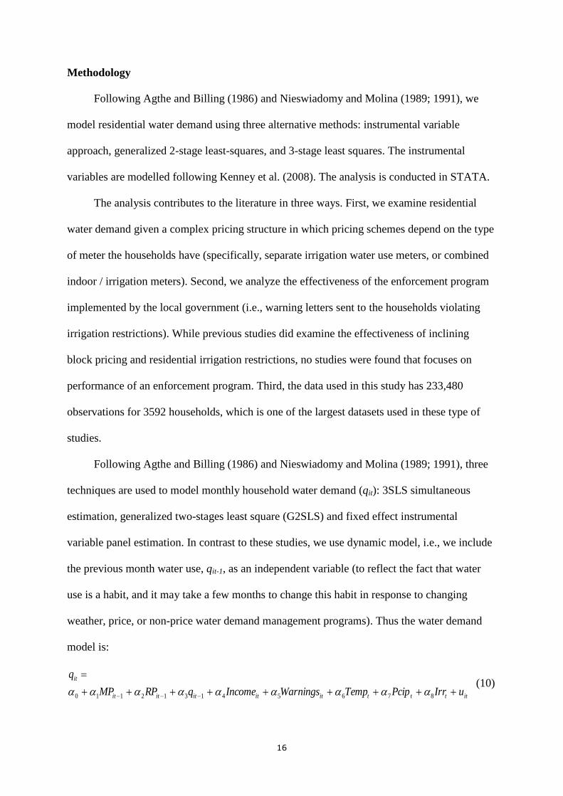
Following Agthe and Billing (1986) and Nieswiadomy and Molina (1989; 1991), we
model residential water demand using three alternative methods: instrumental variable
approach, generalized 2-stage least-squares, and 3-stage least squares. The instrumental
variables are modelled following Kenney et al. (2008). The analysis is conducted in STATA.
The analysis contributes to the literature in three ways. First, we examine residential
water demand given a complex pricing structure in which pricing schemes depend on the type
of meter the households have (specifically, separate irrigation water use meters, or combined
indoor / irrigation meters). Second, we analyze the effectiveness of the enforcement program
implemented by the local government (i.e., warning letters sent to the households violating
irrigation restrictions). While previous studies did examine the effectiveness of inclining
block pricing and residential irrigation restrictions, no studies were found that focuses on
performance of an enforcement program. Third, the data used in this study has 233,480
observations for 3592 households, which is one of the largest datasets used in these type of
studies.
Following Agthe and Billing (1986) and Nieswiadomy and Molina (1989; 1991), three
techniques are used to model monthly household water demand (qit): 3SLS simultaneous
estimation, generalized two-stages least square (G2SLS) and fixed effect instrumental
variable panel estimation. In contrast to these studies, we use dynamic model, i.e., we include
the previous month water use, qit-1, as an independent variable (to reflect the fact that water
use is a habit, and it may take a few months to change this habit in response to changing
weather, price, or non-price water demand management programs). Thus the water demand
model is:
ittttititititit
it
uIrrPcipTempWarningsIncomeqRPMP
q
876541312110 (10)
17
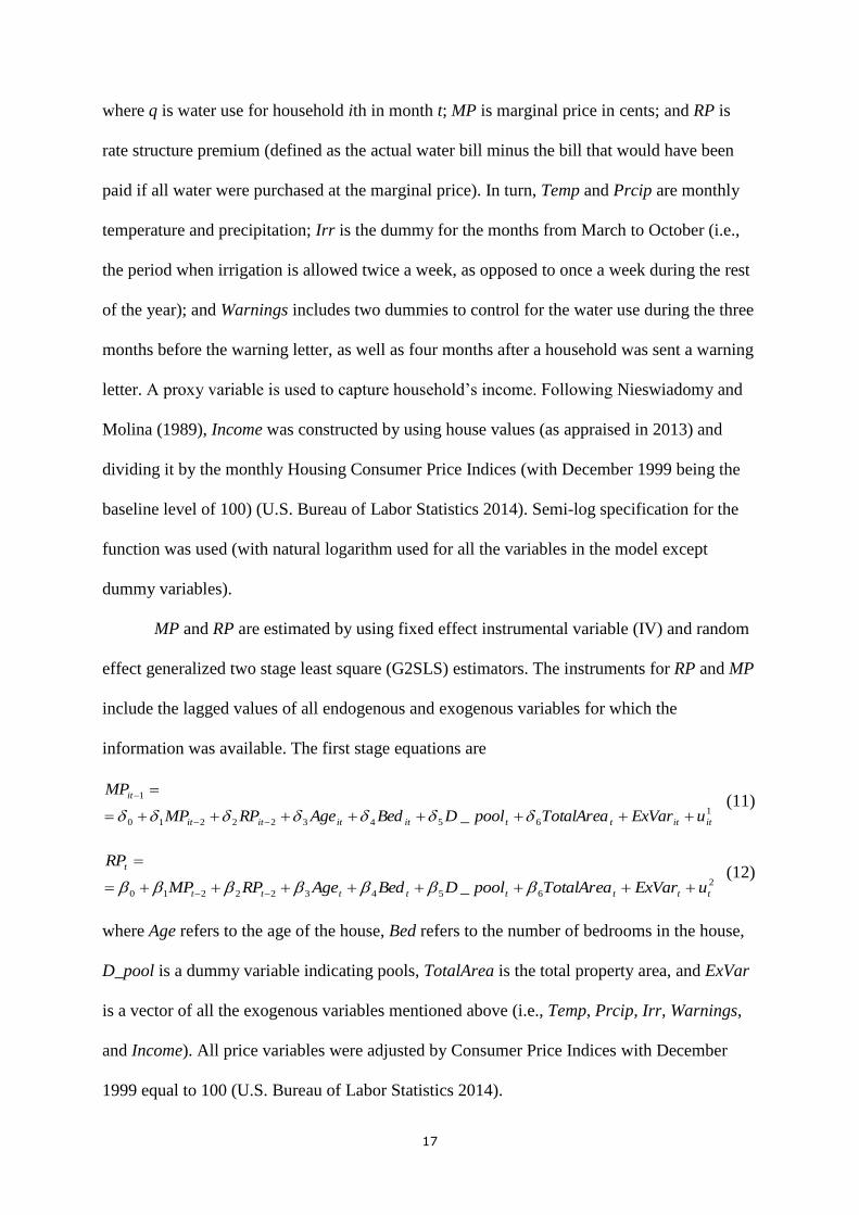
where q is water use for household ith in month t; MP is marginal price in cents; and RP is
rate structure premium (defined as the actual water bill minus the bill that would have been
paid if all water were purchased at the marginal price). In turn, Temp and Prcip are monthly
temperature and precipitation; Irr is the dummy for the months from March to October (i.e.,
the period when irrigation is allowed twice a week, as opposed to once a week during the rest
of the year); and Warnings includes two dummies to control for the water use during the three
months before the warning letter, as well as four months after a household was sent a warning
letter. A proxy variable is used to capture household’s income. Following Nieswiadomy and
Molina (1989), Income was constructed by using house values (as appraised in 2013) and
dividing it by the monthly Housing Consumer Price Indices (with December 1999 being the
baseline level of 100) (U.S. Bureau of Labor Statistics 2014). Semi-log specification for the
function was used (with natural logarithm used for all the variables in the model except
dummy variables).
MP and RP are estimated by using fixed effect instrumental variable (IV) and random
effect generalized two stage least square (G2SLS) estimators. The instruments for RP and MP
include the lagged values of all endogenous and exogenous variables for which the
information was available. The first stage equations are
1
654322210
1
_ ititttitititit
it
uExVarTotalAreapoolDBedAgeRPMP
MP
(11)
2
654322210 _ tttttttt
t
uExVarTotalAreapoolDBedAgeRPMP
RP
(12)
where Age refers to the age of the house, Bed refers to the number of bedrooms in the house,
D_pool is a dummy variable indicating pools, TotalArea is the total property area, and ExVar
is a vector of all the exogenous variables mentioned above (i.e., Temp, Prcip, Irr, Warnings,
and Income). All price variables were adjusted by Consumer Price Indices with December
1999 equal to 100 (U.S. Bureau of Labor Statistics 2014).
18
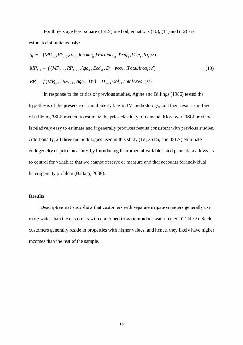
For three stage least square (3SLS) method, equations (10), (11) and (12) are
estimated simultaneously:
);,,,,,,,( 111 tttitititititit IrrPcipTempWarningsIncomeqRPMPfq
);,_,,,,( 221 ttititititit TotalAreapoolDBedAgeRPMPfMP (13)
);,_,,,,( 22 ttititititt TotalAreapoolDBedAgeRPMPfRP .
In response to the critics of previous studies, Agthe and Billings (1986) tested the
hypothesis of the presence of simultaneity bias in IV methodology, and their result is in favor
of utilizing 3SLS method to estimate the price elasticity of demand. Moreover, 3SLS method
is relatively easy to estimate and it generally produces results consistent with previous studies.
Additionally, all three methodologies used in this study (IV, 2SLS, and 3SLS) eliminate
endogeneity of price measures by introducing instrumental variables, and panel data allows us
to control for variables that we cannot observe or measure and that accounts for individual
heterogeneity problem (Baltagi, 2008).
Results
Descriptive statistics show that customers with separate irrigation meters generally use
more water than the customers with combined irrigation/indoor water meters (Table 2). Such
customers generally reside in properties with higher values, and hence, they likely have higher
incomes than the rest of the sample.
19
Table 2. Descriptive Statistics
Variables Units Observations Average Minimum Maximum
Combined Water Use KG/month 196,627.00 8.34 0.00 326.00
Indoor Water Use KG/month 30,356.00 5.13 0.00 200.00
Outdoor Water Use KG/month 30,364.00 11.72 0.00 696.00
Dummy-Warning letter 233,480.00 0.03 0.00 1.00
Average Precipitation Inches/day 233,480.00 0.89 0.00 4.15
Average Temperature Degrees C 233,480.00 20.50 8.80 28.90
House Age years 233,480.00 20.81 0.00 90.00
Number of Bedrooms 233,480.00 3.38 0.00 5.00
Dummy-Pool 233,480.00 0.25 0.00 1.00
Total Area Sq. ft 233,480.00 2,954.30 400.00 20,639.00
Households using combined water meters. Preliminary estimation results for the water
use in the subsample of households with combined meters show that most of the coefficients
in the models are statistically significant and have the expected signs; furthermore, the values
of the coefficients are similar among IV, 2SLS, and 3SLS models. For price elasticity, the
results fall into the lower range of estimates reported in literature, ranging from almost zero
(not statistically significant) in IV model to -0.063 and -0.051 in 2SLS and 3SLS models.
Therefore, given a 10% increase in price the total demand can be expected to decrease by 0%
to 0.6%.
The preliminary results also show that irrigation restriction (i.e., a non-price program)
are effective in reducing water demand. Specifically, the coefficient for dummy_irrigation is
statistically significant and positive, indicating that average water use increases from 9.3
percent to 17.6 percent in the months when irrigation is allowed twice a week (as opposed to
once a week). Note that although the model explicitly accounts for the weather conditions,
additional steps may be required to decouple the effect of weather and irrigation restrictions
on water use. Irrigation restrictions are imposed to reflect weather conditions (i.e., the
restrictions are relaxed to two days per week when the weather is warmer and the
precipitation is higher). Hence, the effect of the restrictions may be masked by the changes in
20
weather. Still, based on our preliminary result, we can speculate that if irrigation is allowed
seven days as opposed to two days a week, the water use can increase by up to (
) times
the estimated percentage, or by 32.6% - 61.6%. This speculative analysis disregards the
reduction in marginal utility from additional water use, and hence, it provides an upper bound
estimate for potential increase in water use that may result in eliminating irrigation
restrictions.
For the inspection component associated with the irrigation restrictions, the coefficient
for one of the dummy variables shows an increase in water use for the households violating
the restrictions. In three months prior to the warning letters, households are estimated to use
14.0% - 14.6% more water per month then their long-term average. Such an increase in water
use shows that warning letters correctly identify and target periods of high water use on
household level. Moreover, descriptive statistics (not reported here) shows that households
receiving the warning letters on average use more water than the averages for their
subdivisions, indicating correct targeting by the County inspection program of the high water
users on subdivision levels. The second dummy variable indicates that in the period 4 months
after the letter, household water use level reduces to pre-peak levels (i.e., to long-term
average), showing that inspection programs are effective. In our sample of households, only
15.6 percent were identified as violating irrigation restrictions (these households were sent
warning letters, 559 out of 3592 households). Hence, even though the program is effective,
the reduction in the total water demand that can be attributed to the inspection program per se
is small in comparison with the potential effect of price increase or changes in the irrigation
restrictions. However, an argument can be made that the effectiveness of the irrigation
restriction program would be smaller in the absence of the inspection component.
The results suggest that households on combined meters do respond to both price- and non-
price water conservation programs examined: irrigation restriction, price increases, and
21
irrigation inspections. Preliminary estimation results show that irrigation restriction can have
higher impact on water use in comparison with modest price increase of 4 to 8 percent
typically used by GRU.
Table 3. Preliminary Estimation Results for Households Using Combined Water Meters
IV G2SLS 3SLS
Intercept -32.810*** -0.672*** -0.746***
(1.914) (0.011) (0.030)
Marginal Price 0.021 -0.063*** -0.051***
(0.017) (0.011) (0.011)
Rate Premium 0.001 -0.042*** -0.009***
(0.002) (0.001) (0.001)
Lag_Usage 0.466*** 0.459*** 0.762***
(0.010) (0.007) (0.007)
Dummy_warning letter
(3 months before letter)
0.140*** 0.140*** 0.146***
(0.014) (0.016) (0.016)
Dummy_warning letter
(4 months after letter)
0.005 -0.010 -0.020
(0.013) (0.014) (0.014)
Property Value 2.801*** 0.125*** 0.094***
(0.159) (0.002) (0.002)
Precipitation -0.041*** -0.053*** -0.054***
(0.002) (0.002) (0.002)
Temperature 0.008*** -0.004*** -0.001**
(0.000) (0.000) (0.000)
Dummy_irrigation 0.093*** 0.192*** 0.176***
(0.004) (0.005) (0.005)
R2 0.24 0.95 0.58
Notes: Asterisks (*, **, ***) represent significant at the 10%, 5% and 1% level, respectively.
Households using separated water meters: indoor water use. Preliminary estimation results
for the households on separate indoor meters show reasonable water demand model fit, with
statistically significant coefficients generally having expected signs. The price elasticity of
demand varies from -0.061 to -0.127 (with 10% significance level). As expected, these
elasticities smaller in absolute value than the elasticities for combined water use discussed
above. Indoor water use primarily includes non-discretionary activities that cannot be adjusted
in response to price change. Dummy variables for warning letters and irrigation restrictions
are mostly not statistically significant. This result is also expected, since the warning letters
22
and restrictions target outdoor water use. Surprisingly, IV model shows a negative and
statistically significant coefficient (-0.05) of the dummy indicating the period of four months
after the warning letters. One can argue that such a letter can remind households about the
need to conserve water, resulting in changes in both indoor and outdoor water use. In
addition, for irrigation restrictions (dummy_irrigation), the coefficient is statistically
significant in G2SLS model (0.020 at the 5% significance level). Similar argument can be
made that changes in irrigation restrictions from one to two days per week may imply that
water conservation is no longer important, influencing household choices both indoor and
outdoor. It is important to note that the coefficients for the variables describing both warning
letters and irrigation restrictions are small, implying marginal changes in indoor water use.
Table 4. Preliminary Estimation Results for Households Using Separate Indoor Water
Meters
IV G2SLS 3SLS
Intercept -21.915*** -0.530*** -0.369***
(3.755) (0.093) (0.092)
Marginal Price -0.061* -0.127*** -0.079***
(0.034) (0.024) (0.024)
Rate Premium -0.053*** -0.047*** -0.028***
(0.004) (0.003) (0.002)
Lag_Usage 0.137*** 0.497*** 0.659***
(0.017) (0.010) (0.009)
Dummy_warning letter
(3 months earlier)
-0.022 0.009 0.001
(0.024) (0.026) (0.025)
Dummy_warning letter
(4 months later)
-0.050** -0.006 -0.016
(0.021) (0.023) (0.022)
Property Value 1.838*** 0.106*** 0.073***
(0.296) (0.007) (0.007)
Precipitation -0.010** -0.017*** -0.016***
(0.004) (0.004) (0.004)
Temperature -0.001 -0.002** -0.001
(0.001) (0.001) (0.001)
Dummy_irrigation 0.010 0.020** 0.008
(0.009) (0.009) (0.009)
R2 0.06 0.90 0.45
Notes: Asterisks (*, **, ***) represent significant at the 10%, 5% and 1% level, respectively.
23
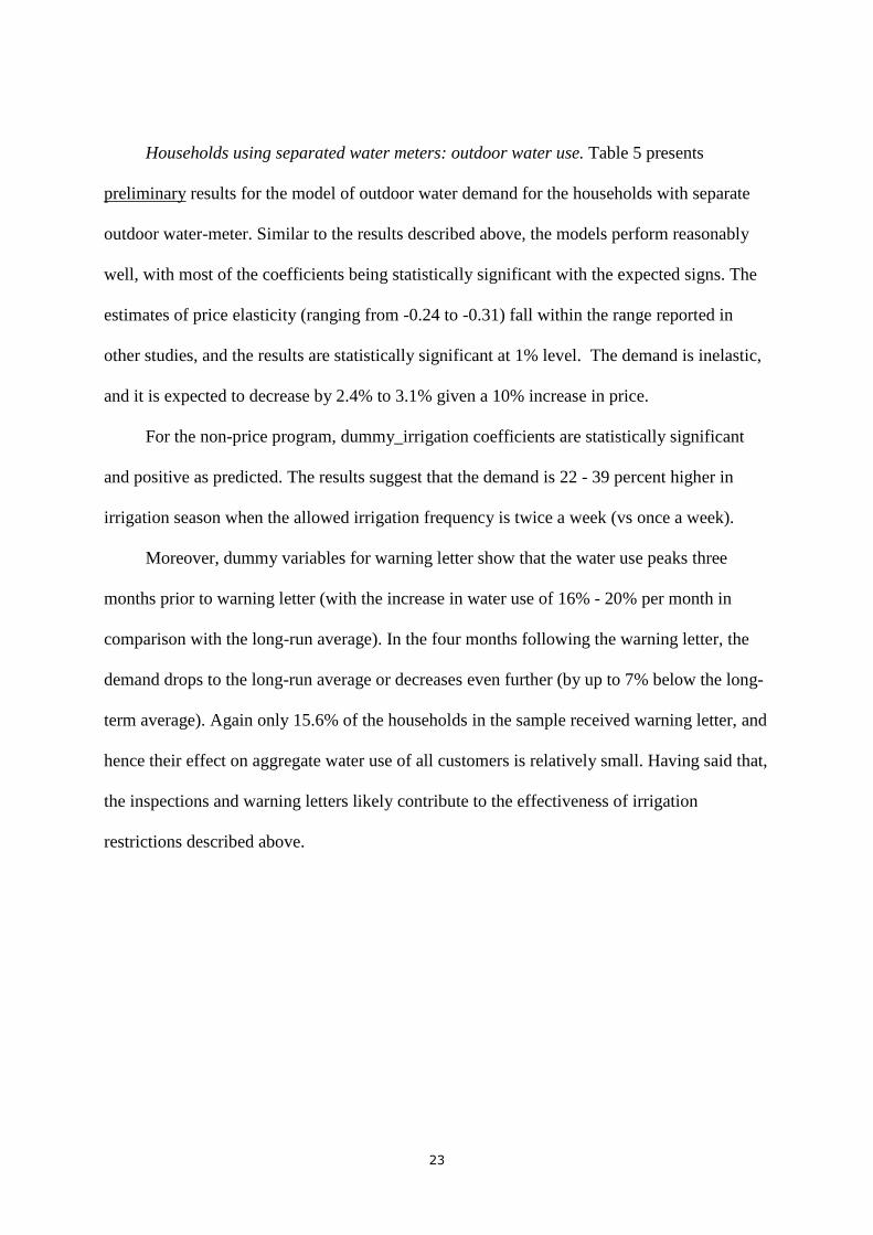
Households using separated water meters: outdoor water use. Table 5 presents
preliminary results for the model of outdoor water demand for the households with separate
outdoor water-meter. Similar to the results described above, the models perform reasonably
well, with most of the coefficients being statistically significant with the expected signs. The
estimates of price elasticity (ranging from -0.24 to -0.31) fall within the range reported in
other studies, and the results are statistically significant at 1% level. The demand is inelastic,
and it is expected to decrease by 2.4% to 3.1% given a 10% increase in price.
For the non-price program, dummy_irrigation coefficients are statistically significant
and positive as predicted. The results suggest that the demand is 22 - 39 percent higher in
irrigation season when the allowed irrigation frequency is twice a week (vs once a week).
Moreover, dummy variables for warning letter show that the water use peaks three
months prior to warning letter (with the increase in water use of 16% - 20% per month in
comparison with the long-run average). In the four months following the warning letter, the
demand drops to the long-run average or decreases even further (by up to 7% below the long-
term average). Again only 15.6% of the households in the sample received warning letter, and
hence their effect on aggregate water use of all customers is relatively small. Having said that,
the inspections and warning letters likely contribute to the effectiveness of irrigation
restrictions described above.
24
Table 5. Preliminary Estimation Results for Households Using Separate Outdoor Water
Meters
IV G2SLS 3SLS
Intercept -33.031*** 0.082 -0.861***
(7.281) (0.245) (0.243)
Marginal Price -0.242*** -0.306*** -0.239***
(0.084) (0.069) (0.068)
Rate Premium -0.012*** -0.031*** -0.006**
(0.004) (0.002) (0.002)
Lag_Usage 0.292*** 0.223*** 0.715***
(0.046) (0.035) (0.034)
Dummy_warning letter
(3 months earlier)
0.188*** 0.198*** 0.162***
(0.042) (0.046) (0.044)
Dummy_warning letter
(4 months later)
-0.016 -0.010 -0.069*
(0.038) (0.041) (0.039)
Property Value 2.747*** 0.137*** 0.133***
(0.569) (0.016) (0.016)
Precipitation -0.069*** -0.083*** -0.076***
(0.007) (0.008) (0.008)
Temperature 0.008*** -0.006*** -0.005***
(0.002) (0.002) (0.002)
Dummy_irrigation 0.216*** 0.344*** 0.389***
(0.019) (0.022) (0.021)
R2 0.19 0.84 0.39
Notes: Asterisks (*, **, ***) represent significant at the 10%, 5% and 1% level, respectively.
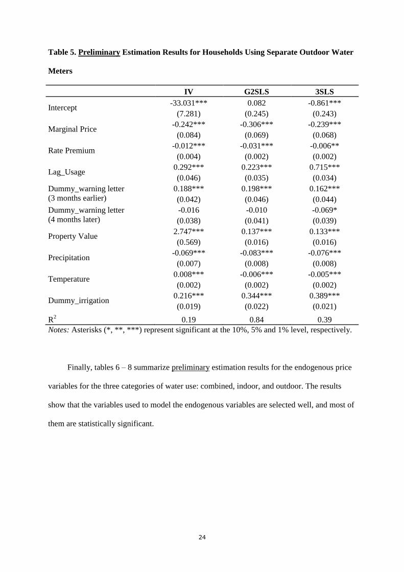
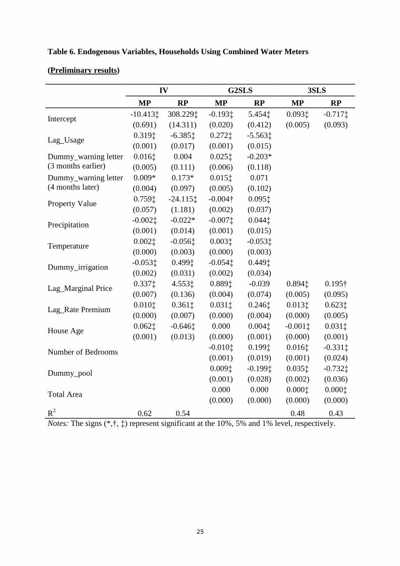
Finally, tables 6 – 8 summarize preliminary estimation results for the endogenous price
variables for the three categories of water use: combined, indoor, and outdoor. The results
show that the variables used to model the endogenous variables are selected well, and most of
them are statistically significant.
25
Table 6. Endogenous Variables, Households Using Combined Water Meters
(Preliminary results)
IV G2SLS 3SLS
MP RP MP RP MP RP
Intercept -10.413‡ 308.229‡ -0.193‡ 5.454‡ 0.093‡ -0.717‡
(0.691) (14.311) (0.020) (0.412) (0.005) (0.093)
Lag_Usage 0.319‡ -6.385‡ 0.272‡ -5.563‡
(0.001) (0.017) (0.001) (0.015) Dummy_warning letter
(3 months earlier)
0.016‡ 0.004 0.025‡ -0.203* (0.005) (0.111) (0.006) (0.118) Dummy_warning letter
(4 months later)
0.009* 0.173* 0.015‡ 0.071 (0.004) (0.097) (0.005) (0.102)
Property Value 0.759‡ -24.115‡ -0.004† 0.095‡
(0.057) (1.181) (0.002) (0.037)
Precipitation -0.002‡ -0.022* -0.007‡ 0.044‡
(0.001) (0.014) (0.001) (0.015)
Temperature 0.002‡ -0.056‡ 0.003‡ -0.053‡
(0.000) (0.003) (0.000) (0.003)
Dummy_irrigation -0.053‡ 0.499‡ -0.054‡ 0.449‡
(0.002) (0.031) (0.002) (0.034)
Lag_Marginal Price 0.337‡ 4.553‡ 0.889‡ -0.039 0.894‡ 0.195†
(0.007) (0.136) (0.004) (0.074) (0.005) (0.095)
Lag_Rate Premium 0.010‡ 0.361‡ 0.031‡ 0.246‡ 0.013‡ 0.623‡
(0.000) (0.007) (0.000) (0.004) (0.000) (0.005)
House Age 0.062‡ -0.646‡ 0.000 0.004‡ -0.001‡ 0.031‡
(0.001) (0.013) (0.000) (0.001) (0.000) (0.001)
Number of Bedrooms
-0.010‡ 0.199‡ 0.016‡ -0.331‡
(0.001) (0.019) (0.001) (0.024)
Dummy_pool
0.009‡ -0.199‡ 0.035‡ -0.732‡
(0.001) (0.028) (0.002) (0.036)
Total Area
0.000 0.000 0.000‡ 0.000‡
(0.000) (0.000) (0.000) (0.000)
R2 0.62 0.54 0.48 0.43
Notes: The signs (*,†, ‡) represent significant at the 10%, 5% and 1% level, respectively.
26
Table 7. Endogenous Variables, Households Using Separate Indoor Water Meters
(Preliminary results)
IV G2SLS 3SLS
MP RP MP RP MP RP
Intercept -4.437‡ 1.551 0.414‡ -8.106‡ -0.029‡ 1.239‡
(1.396) (29.325) (0.063) (1.321) (0.008) (0.173)
Lag_Usage 0.195‡ -4.164‡ 0.149‡ -3.228‡
(0.002) (0.044) (0.002) (0.036) Dummy_warning letter
(3 months earlier)
0.009 -0.168 -0.006 0.165 (0.008) (0.172) (0.009) (0.181) Dummy_warning letter
(4 months later)
0.012* -0.109 -0.001 0.193 (0.007) (0.152) (0.008) (0.158)
Property Value 0.308‡ 0.518 -0.053‡ 1.166‡
(0.110) (2.303) (0.005) (0.114)
Precipitation -0.006‡ -0.015 -0.008‡ 0.001
(0.001) (0.027) (0.001) (0.029)
Temperature 0.001‡ -0.018‡ 0.002‡ -0.025‡
(0.000) (0.005) (0.000) (0.006)
Dummy_irrigation -0.045‡ 0.310‡ -0.048‡ 0.363‡
(0.003) (0.061) (0.003) (0.066)
Lag_Marginal Price 0.636‡ 0.658* 1.016‡ -1.539‡ 1.009‡ -1.090‡
(0.018) (0.381) (0.008) (0.158) (0.008) (0.175)
Lag_Rate Premium 0.020‡ 0.241‡ 0.031‡ 0.270‡ 0.023‡ 0.472‡
(0.001) (0.018) (0.000) (0.009) (0.000) (0.010)
House Age 0.037‡ -0.214‡ 0.000† -0.003 0.000 0.002
(0.002) (0.035) (0.000) (0.003) (0.000) (0.003)
Number of Bedrooms
0.000 0.008 0.006‡ -0.126‡
(0.002) (0.036) (0.002) (0.039)
Dummy_pool
-0.001 0.006 0.001 -0.026
(0.002) (0.045) (0.002) (0.047)
Total Area
0.000‡ 0.000‡ 0.000‡ 0.000‡
(0.000) (0.000) (0.000) (0.000)
R2 0.58 0.34 0.50 0.29
Notes: The signs (*,†, ‡) represent significant at the 10%, 5% and 1% level, respectively.
27
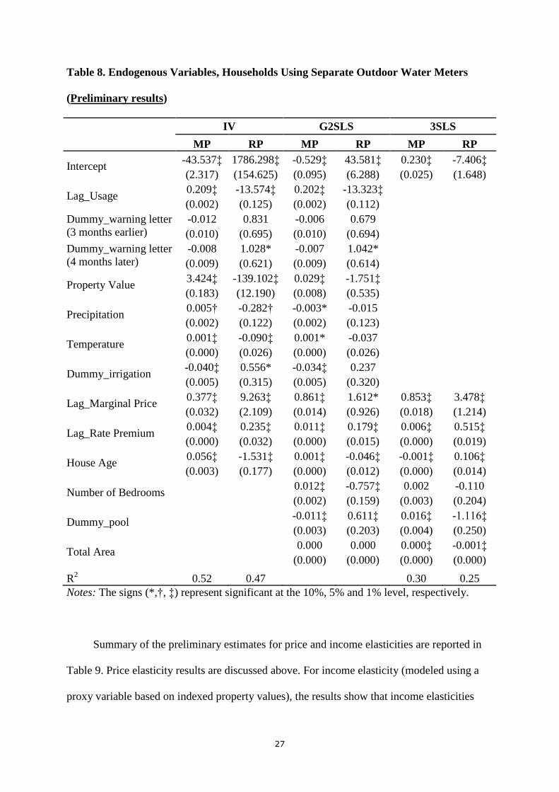
Table 8. Endogenous Variables, Households Using Separate Outdoor Water Meters
(Preliminary results)
IV G2SLS 3SLS
MP RP MP RP MP RP
Intercept -43.537‡ 1786.298‡ -0.529‡ 43.581‡ 0.230‡ -7.406‡
(2.317) (154.625) (0.095) (6.288) (0.025) (1.648)
Lag_Usage 0.209‡ -13.574‡ 0.202‡ -13.323‡
(0.002) (0.125) (0.002) (0.112) Dummy_warning letter
(3 months earlier)
-0.012 0.831 -0.006 0.679 (0.010) (0.695) (0.010) (0.694) Dummy_warning letter
(4 months later)
-0.008 1.028* -0.007 1.042* (0.009) (0.621) (0.009) (0.614)
Property Value 3.424‡ -139.102‡ 0.029‡ -1.751‡
(0.183) (12.190) (0.008) (0.535)
Precipitation 0.005† -0.282† -0.003* -0.015
(0.002) (0.122) (0.002) (0.123)
Temperature 0.001‡ -0.090‡ 0.001* -0.037
(0.000) (0.026) (0.000) (0.026)
Dummy_irrigation -0.040‡ 0.556* -0.034‡ 0.237
(0.005) (0.315) (0.005) (0.320)
Lag_Marginal Price 0.377‡ 9.263‡ 0.861‡ 1.612* 0.853‡ 3.478‡
(0.032) (2.109) (0.014) (0.926) (0.018) (1.214)
Lag_Rate Premium 0.004‡ 0.235‡ 0.011‡ 0.179‡ 0.006‡ 0.515‡
(0.000) (0.032) (0.000) (0.015) (0.000) (0.019)
House Age 0.056‡ -1.531‡ 0.001‡ -0.046‡ -0.001‡ 0.106‡
(0.003) (0.177) (0.000) (0.012) (0.000) (0.014)
Number of Bedrooms
0.012‡ -0.757‡ 0.002 -0.110
(0.002) (0.159) (0.003) (0.204)
Dummy_pool
-0.011‡ 0.611‡ 0.016‡ -1.116‡
(0.003) (0.203) (0.004) (0.250)
Total Area
0.000 0.000 0.000‡ -0.001‡
(0.000) (0.000) (0.000) (0.000)
R2 0.52 0.47 0.30 0.25
Notes: The signs (*,†, ‡) represent significant at the 10%, 5% and 1% level, respectively.
Summary of the preliminary estimates for price and income elasticities are reported in
Table 9. Price elasticity results are discussed above. For income elasticity (modeled using a
proxy variable based on indexed property values), the results show that income elasticities
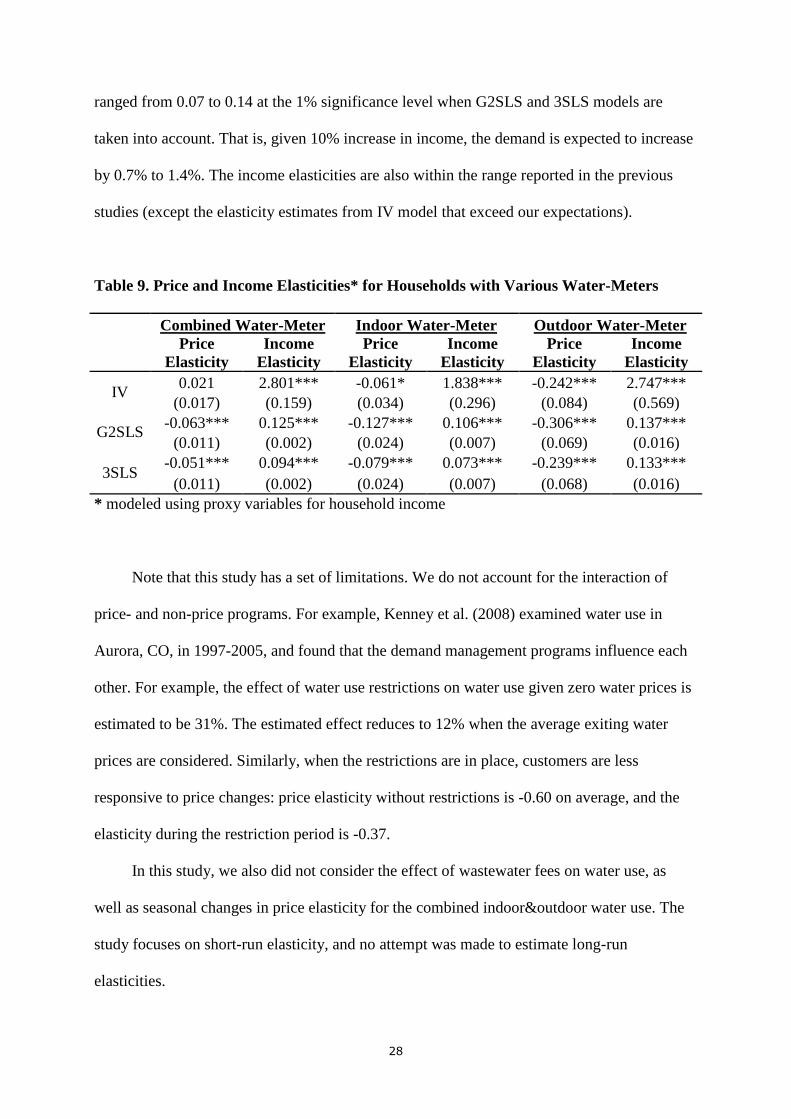
28
ranged from 0.07 to 0.14 at the 1% significance level when G2SLS and 3SLS models are
taken into account. That is, given 10% increase in income, the demand is expected to increase
by 0.7% to 1.4%. The income elasticities are also within the range reported in the previous
studies (except the elasticity estimates from IV model that exceed our expectations).
Table 9. Price and Income Elasticities* for Households with Various Water-Meters
Combined Water-Meter Indoor Water-Meter Outdoor Water-Meter
Price
Elasticity
Income
Elasticity
Price
Elasticity
Income
Elasticity
Price
Elasticity
Income
Elasticity
IV 0.021 2.801*** -0.061* 1.838*** -0.242*** 2.747***
(0.017) (0.159) (0.034) (0.296) (0.084) (0.569)
G2SLS -0.063*** 0.125*** -0.127*** 0.106*** -0.306*** 0.137***
(0.011) (0.002) (0.024) (0.007) (0.069) (0.016)
3SLS -0.051*** 0.094*** -0.079*** 0.073*** -0.239*** 0.133***
(0.011) (0.002) (0.024) (0.007) (0.068) (0.016)
* modeled using proxy variables for household income
Note that this study has a set of limitations. We do not account for the interaction of
price- and non-price programs. For example, Kenney et al. (2008) examined water use in
Aurora, CO, in 1997-2005, and found that the demand management programs influence each
other. For example, the effect of water use restrictions on water use given zero water prices is
estimated to be 31%. The estimated effect reduces to 12% when the average exiting water
prices are considered. Similarly, when the restrictions are in place, customers are less
responsive to price changes: price elasticity without restrictions is -0.60 on average, and the
elasticity during the restriction period is -0.37.
In this study, we also did not consider the effect of wastewater fees on water use, as
well as seasonal changes in price elasticity for the combined indoor&outdoor water use. The
study focuses on short-run elasticity, and no attempt was made to estimate long-run
elasticities.
29
Conclusion
Preliminary results show that the panel data regression models used to examine water
demand have good fit, and most of the variables have expected and statistically significant
effects on water use. Implementing residential irrigation restrictions, irrigation inspection
program, and price increases have a significant negative effect on monthly water use.
When price elasticity results are examined across the three models and for different
water use categories (combined, indoor, and outdoor), it can be seen that outdoor use is most
responsive to price changes. However, even for this category of water use, 10 percent increase
in price is estimated to induce only 3 percent reduction in water use. In other words, to
achieve 10 percent reduction in use, prices should be increased by 30 percent or more. Given
that currently the maximum GRU water rate is $6 for a thousand gallon, such an increase
would results in rates above $10 per thousand gallons. While this increase may not be
politically feasible in Florida, it is not unrealistic. For example, in Austin, TX, the maximum
price charged for water use about 20 thousand gallons is $12.55 per thousand gallons (Austin
Water Utility 2013). Political feasibility of price increase can be improved by focusing on
high price blocks only.
Irrigation restrictions are also effective in curbing water use (even though the effects of
weather and irrigation restrictions can be difficult to decouple). Changing allowed irrigation
frequency from once a week to twice a week results in up to 40 percent increase in water use.
Irrigation inspections likely contribute to effectiveness of the irrigation restrictions in Alachua
County.
Comprehensive economic analyses of residential water demand is of great need for
water utility companies and local and state agencies implementing a variety of residential
water conservation programs. These study results can help increase effectiveness of such
30
programs, and select price and non-price programs that lead to the expected water use change
for the residential customers.
References
Agthe, D.E., B.R. Billings, J.L. Dobra, and K.Raffiee. 1986. “A Simultaneous Equation Model for Block
Rates.” Water Resources Research 22 (1): 1-4.
Arizona Department of Water Resources. 2014. Outdoor Residential Water Conservation.
http://www.azwater.gov/azdwr/StatewidePlanning/Conservation2/Residential/Outdoor_Residential_Cons
ervation.htm (accessed on May 20, 2014).
Austin Water Utility. 2013. Approved Water Service Rates - Retail Customers (Effective November 1, 2013).
http://www.austintexas.gov/department/austin-water-utility-service-rates (accessed on May 28, 2014).
Billings, R. B,, and Donald E. Agthe. 1980. “Price Elasticities for Water: A Case of In-creasing Block Rates.”
Land Economics 56 (1):73-84.
Brennan D., S. Tapsuwan, and G. Ingram. 2007. “The Welfare Costs of Urban Outdoor Water Restrictions.” The
Australian Journal of Agricultural and Resource Economics 51, 243-261.
Borisova, T., and P. Useche. 2013. “Exploring The Effects of Extension Workshops on Household Water-use
Behavior.” Horticultural Technology 23:668-676.
Dalhuisen, J.M., R.J.G.M. Florax, H. de Groot, and P. Nijkamp. 2003. “Price and Income Elasticities of
Residential Water Demand: A Meta-analysis.” Land Economics 79(2): 292–308.
Espey, M., J. Espey, and W.D. Shaw. 1997. “Price Elasticity of Residential Demand for Water: A Meta-
analysis.” Water Resources Research 33(6), 1369–1374.
Foster, Henry S., Jr., and Bruce Beattie. 1979. “Urban Residential Demand for Water in the United States.” Land
Economics 55 (1): 43-58.
Friedman, K., Heaney, J., Morales, M. and J. Palenchar. 2013. “Predicting and Managing Residential Potable
Irrigation Using Parcel Level Databases.” Journal of the American Water Works Association 105(7):
Garcia-Valinas, M. (2006). “Analysing rationing policies: drought and its effects on urban users’ welfare.”
Applied Economics 38: 955–965.
Gottlieb, M. 1963. “Urban Domestic Demand for Water: A Kansas Study.” Land Economics 39 (2): 204-210.
Haney, M.B., M.D. Dukes, and G.L. Miller. 2007. “Residential irrigation water use in Central Florida.” Journal
of Irrigation and Drainage Engineering, September/October:427-434.
31
Hermitte, S.M., and R.E. Mace. 2012. “The Grass Is Always Greener…Outdoor Residential Water Use in
Texas.” Texas Water Development Board Technical Note 12-01, November.
https://www.twdb.state.tx.us/publications/reports/technical_notes/doc/SeasonalWaterUseReport-final.pdf
Hewitt, J., and M. Hanemann. 1995, “A Discrete/Continuous Choice Approach to Residential Water Demand
under Block Rate Pricing,” Land Economics 71(2): 173-192.
Howe, C.W., and C. Goemans. 2002. “Effectiveness of Water Rate Increases Following Watering Restrictions.”
Journal of American Water Resources Association 94(10): 28-32.
Howe, C.W. and F. P. Linaweaver, Jr. 1967. “The Impact of Price on Residential Water Demand and Its Relation
to System Design and Price Structure.” Water Resources Research 3(1): 13-32.
House-Peters, L.A., and H. Chang. 2011. “Urban Water Demand Modeling: Review of Concepts, Methods, and
Organizing Principles.” Water Resources Research 47():
Kenney, D.S., R.A. Klein, and M.P. Clark. 2004. “Use and Effectiveness of Municipal Water Restrictions
During Drought in Colorado.” Journal of American Water Resources Association 40(1): 77-87.
Kenney, D.S., C. Goemans, R. Klein, J. Lowrey, and K. Reidy. 2008. “Residential Water Demand Management:
Lessons from Aurora, Colorado.” Journal of American Water Resources Association 44(1):192–207.
Kenny, J.F., N.L. Barber, S.S. Hutson, K.S. Linsey, J.K. Lovelace, and M.A. Maupin. 2009. “Estimated Use of
Water in the United States in 2005.” U.S. Geological Survey Circular 1344, 52 p.
http://pubs.usgs.gov/circ/1344/pdf/c1344.pdf
Klaiber, H.A., V.K. Smith, M. Kaminsky, and A. Strong. 2012. “Measuring Price Elasticities for Residential
Water Demand with Limited Information.” Working paper, Carey School of Business, Arizona State
University.
Lee, M.Y. 1981. “Mandatory or Voluntary Water Conservation: A case Study of Iowa Communities During
Drought.” Journal of Soil and Water Conservation 36(4): 231-234.
Lee, M.Y. and R.D. Warren. 1981. “Use of Predictive Model in Evaluating Water Consumption Conservation.”
Water Resources Bulletin 17(6): 948-955.
Moncur, J., 1987. “Urban Water Pricing and Drought Management, Water Resources Research, 23: 393–8.
Michelsen, A.M., J.T. McGuckin, and D. Stumpf. 1999. “Nonprice Water Conservation Programs as a Demand
Management Tool.” Journal of American Water Resources Association, 35(3): 593-602.
Nataraj, S., and W.M. Hanemann. 2011. “Does Marginal Price Matter? A Regression Discontinuity Approach to
Estimating Water Demand.” Journal of Environmental Economics and Management 61: 198–212.
32
Olmstead, S.M., W.M. Hanemann and R.N. Stavis. 2007. “Water demand under alternative price structures.”
Journal of Environmental Economics and Management, 54 (1): 181–198
Olmstead, S.M., and R.N. Stavis. 2007. “Comparing price and nonprice approaches to urban water
conservation.” Water Resources Research 45: 1-10.
Ozan L.A. and K.A. Alsharif. 2013. “The Effectiveness of Water Irrigation Policies for Residential Turfgrass.”
Land Use Policy, 21(1): 378-384.
Pint, E.M. 1999. “Household Responses to Increased Water Rates during the California Drought.” Land
Economics 75 (2): 246–266.
Rensick, M.E., and R.D. Green. 2000. “Do Residential Water Demand Management Policies Measure Up? An
Analysis of Eight California Water Agencies.” Journal of Environmental Economics and Management,
40(1):37-55.
Renwick, M.E., and S.O. Archibald. 1998 . “Demand Side Management Policies for Residential Water Use:
Who Bears The Conservation Burden?” Land Economics 74(3), 343–359.
Schuck, E.C., and R. Profit. 2004. “Evaluating Non-price Water Demand Policies during Severe Droughts.”
Selected Paper ” Paper presented at the American Agricultural Economics Association Annual Meeting,
Denver, Colorado, July 1–4.
Shaw, D.T., and D.R. Maidment. 1987. “Intervention Analysis of Water Use Restrictions, Austin, Texas.” Water
Resources Bulletin, 23 (6): 1037-1046
Shaw, D.T., and D.R. Maidment. 1988. “Effects of Conservation on Daily Water Use.” Journal of American
Water Resources Association, 80(9): 71-77.
Syme, G.J., B.E. Nancarrow, and C. Seligman. 2000. “The evaluation of information campaigns to promote
voluntary household water conservation.” Evaluation Review 24:539–578.
Nieswiadomy, M.L. 1992. “Estimating urban residential water demand, Effects of Price Structure, Conservation
and Education.” Water Resources Research 28: 609–615.
Nieswiadomy M.L., and D.J. Molina. 1989. “Comparing Residential Water Demand Estimates under Decreasing
and Increasing Block Rates.” Land Economics 65(3): 280-289.
Nieswiadomy M.L., and D.J. Molina. 1991. “A Note on Price Perception in Water Demand Models.” Land
Economics 67(3): 352-359.
Nordin, J. A. 1976. “A Proposed Modification of Taylor's Demand Analysis: Comment.” The Bell Journal of
Economics 7 (2): 719-21.
33
Southwest Florida Water Management District. Undated. Saving Water Outdoors.
http://www.swfwmd.state.fl.us/conservation/outdoors/
South Florida Water Management District. 2008. Water Conservation: A Comprehensive Program for South
Florida. South Florida Water Management District, West Palm Beach, FL.
www.sfwmd.gov/portal/page/portal/xrepository/sfwmd_repository_pdf/waterconservationplan.pdf
Taylor, L.D. 1975. “The Demand for Electricity: A Survey.” The Bell Journal of Economics 6 (1): 74-110.
Wong, S. T. 1972. “A Model on Municipal Water Demand: A Case Study of Northeastern Illinois.” Land
Economics 48 (1): 34-44.
Woo, C. 1994. “Managing water supply shortage. Interruption vs. pricing,” Journal of Public Economics 54:
145–60.
Yoo J., S.Simonit, A.P. Kinzig, and C. Perrings, 2014. “Estimating the Price Elasticity of Residential Water
Demand: The Case of Phoenix, Arizona.” Applied Economic Perspectives and Policy 36(2): 333-350.
Young, R.A. 1973. “Price Elasticity of Demand for Municipal Water: Case Study of Tucson, Arizona.” Water
Resources Research 9 (Aug.): 1068-72.